NetGAN: Generating Graphs via Random Walks · nary indicators, counts) in patient records. ... The goal of the generator is to generate synthetic random walks that are plausible in

NetGAN: Generating Graphs via Random Walks

Aleksandar Bojchevski * 1 Oleksandr Shchur * 1 Daniel Zugner * 1 Stephan Gunnemann 1

Abstract

We propose NetGAN – the first implicit genera-tive model for graphs able to mimic real-worldnetworks. We pose the problem of graph genera-tion as learning the distribution of biased randomwalks over the input graph. The proposed modelis based on a stochastic neural network that gener-ates discrete output samples and is trained usingthe Wasserstein GAN objective. NetGAN is ableto produce graphs that exhibit well-known net-work patterns without explicitly specifying themin the model definition. At the same time, ourmodel exhibits strong generalization properties,as highlighted by its competitive link predictionperformance, despite not being trained specifi-cally for this task. Being the first approach tocombine both of these desirable properties, Net-GAN opens exciting avenues for further research.

1. IntroductionGenerative models for graphs have a longstanding history,with applications including data augmentation, anomalydetection and recommendation (Chakrabarti & Faloutsos,2006). Explicit probabilistic models such as Barabasi-Albertor stochastic blockmodels are the de-facto standard in thisfield (Goldenberg et al., 2010). However, it has also beenshown on multiple occasions that our intuitions about struc-ture and behavior of graphs may be misleading. For in-stance, heavy-tailed degree distributions in real graphs werein strong disagreement with the models existing at the timeof their discovery (Barabasi & Albert, 1999). More recentworks like Dong et al. (2017) and Broido & Clauset (2018)keep bringing up other surprising characteristics of real-world networks that question the validity of the establishedmodels. This leads us to the question: “How do we de-fine a model that captures all the essential (potentially stillunknown) properties of real graphs?”

*Equal contribution 1Technical University of Munich, Germany.Correspondence to: Daniel Zugner <[email protected]>.

Proceedings of the 35 th International Conference on MachineLearning, Stockholm, Sweden, PMLR 80, 2018. Copyright 2018by the author(s).

An increasingly popular way to address this issue in otherfields is by switching from explicit (prescribed) models toimplicit ones. This transition is especially notable in com-puter vision, where generative adversarial networks (GANs)(Goodfellow et al., 2014) significantly advanced the stateof the art over the classic prescribed approaches like mix-tures of Gaussians (Blanken et al., 2007). GANs achieveunparalleled results in scenarios such as image and 3D ob-jects generation (e.g., Karras et al., 2017; Berthelot et al.,2017; Wu et al., 2016). However, despite their massive suc-cess when dealing with real-valued data, adapting GANsto handle discrete objects like graphs or text remains anopen research problem (Goodfellow, 2016). In fact, dis-creteness is only one of the obstacles when applying GANsto network data. Large repositories of graphs that all comefrom the same distribution are not available. This meansthat in a typical setting one has to learn from a single graph.Additionally, any model operating on a graph necessarilyhas to be permutation invariant, as graphs are isomorphicunder node reordering.

In this work we introduce NetGAN – the first implicit gener-ative model for graphs and networks that tackles all of theabove challenges. We formulate the problem of learning thegraph topology as learning the distribution of biased randomwalks over the graph. Like in the typical GAN setting, thegenerator G – in our case defined as a stochastic neuralnetwork with discrete output samples – learns to generaterandom walks that are plausible in the real graph, while thediscriminator D then has to distinguish them from the trueones that are sampled from the original graph.

The main requirement for a graph generative model is theability to generate realistic graphs. In the experimentalsection we compare NetGAN to other established prescribedmodels on this task. We observe that our proposed methodconsistently reproduces most known patterns inherent toreal-world networks without explicitly specifying any ofthem in the model definition (e.g., degree distribution, asseen in Fig. 1). However, a model that simply replicates theoriginal graph would also trivially fulfill this requirement,which clearly isn’t our goal. In order to prove that thisis not the case we examine the generalization propertiesof NetGAN by evaluating its link prediction performance.As our experiments show, our model exhibits competitiveperformance in this task and even achieves state-of-the-art

arX

iv:1

803.

0081

6v2

[st

at.M

L]

1 J

un 2

018


(a) Original graph

44% edgeoverlap

(b) Graph generated by NetGAN

100 101 102

Degree

100

101

102

Num

ber

of

nod

es

Citeseer

NetGAN

(c) Degree distribution comparison

Figure 1: (a) Subgraph of the CITESEER network and (b) the respective subset of the graph generated by NetGAN. Bothhave similar structure but are not identical. (c) shows that the degree distributions of the two graphs are very close.

results on some datasets. This result is especially impressive,since NetGAN is not trained explicitly for performing linkprediction. To summarize, our main contributions are:

• We introduce NetGAN1 – the first of its kind GANarchitecture that generates graphs via random walks.Our model tackles the associated challenges of stayingpermutation invariant, learning from a single graph andgenerating discrete output.

• We show that our method preserves important topolog-ical properties, without having to explicitly specifyingthem in the model definition. Moreover, we demon-strate how latent space interpolation leads to producinggraphs with smoothly changing characteristics.

• We highlight the generalization properties of NetGANby its link prediction performance that is competitivewith the state of the art on real-word datasets, despitethe model not being trained explicitly for this task.

2. Related WorkSo far, no GAN architectures applicable to real-world net-works have been proposed. Liu et al. (2017) propose a GANarchitecture for learning topological features of subgraphs.Tavakoli et al. (2017) apply GANs to graph data by trying todirectly generate adjacency matrices. Because their modelproduces the entire adjacency matrix – including the zeroentries – it requires computations and memory quadratic inthe number of nodes. Such quadratic complexity is infeasi-ble in practice, allowing to process only small graphs, withreported runtime of over 60 hours for a graph with only 154nodes. In contrast, NetGAN operates on random walks – itconsiders only the non-zero entries of the adjacency matrixefficiently exploiting the sparsity of real-world graphs – andis readily applicable to graphs with thousands of nodes.

1 Code available at: https://www.kdd.in.tum.de/netgan

Deep learning methods for graph data have mostly beenstudied in the context of node embeddings (Perozzi et al.,2014; Grover & Leskovec, 2016; Kipf & Welling, 2016).The main idea behind these approaches is that of model-ing the probabilities of each individual edge’s existence,p(Auv), as some function of the respective node embed-dings, f(hu,hv), where f is represented by a neural net-work. The recently proposed GraphGAN (Wang et al., 2017)is another instance of such prescribed edge-level probabilis-tic models, where f is optimized using the GAN objectiveinstead of the traditional cross-entropy. Deep embeddingbased methods achieve state-of-the-art scores in tasks likelink prediction and node classification. Nevertheless, aswe show in Sec. 3.2, using such approaches for generatingentire graphs produces samples that don’t preserve any ofthe patterns inherent to real-world networks.

Prescribed generative models for graphs have a long his-tory and are well-studied. For a survey we refer the readerto Chakrabarti & Faloutsos (2006) and Goldenberg et al.(2010). Typically, prescribed generative approaches are de-signed to capture and reproduce some predefined subsetof graph properties (e.g., degree distribution, communitystructure, clustering coefficient). Notable examples includethe configuration model (Bender & Canfield, 1978; Molloy& Reed, 1995), variants of the degree-corrected stochas-tic blockmodel (Karrer & Newman, 2011; Bojchevski &Gunnemann), Exponential Random Graph Models (Holland& Leinhardt, 1981), Multiplicative Attribute Graph model(Kim & Leskovec, 2011), and the block two-level Erdos-Reniy random graph model (Seshadhri et al., 2012). InSec. 4 we compare with some of these prescribed modelson the tasks of graph generation and link prediction.

Due to the challenging nature of the problem, only few ap-proaches able to generate discrete data using GANs exist.Most approaches focus on generating discrete sequencessuch as text, with some of them using reinforcement learn-

https://www.kdd.in.tum.de/netgan


ing techniques to enable backpropagation through sam-pling discrete random variables (Yu et al., 2017; Kusner& Hernandez-Lobato, 2016; Li et al., 2017; Liang et al.,2017). Other approaches modify the GAN objective totackle the same challenge (Che et al., 2017; Hjelm et al.,2017). Focusing on non-sequential discrete data, Choi et al.(2017) generate high-dimensional discrete features (e.g. bi-nary indicators, counts) in patient records. None of thesemethods have considered graph structured data.

3. ModelIn this section we introduce NetGAN - a Generative Ad-versarial Network model for graph / network data. Its coreidea lies in capturing the topology of a graph by learn-ing a distribution over the random walks. Given an inputgraph of N nodes, defined by a binary adjacency matrixA ∈ 0, 1N×N , we first sample a set of random walks oflength T from A. This collection of random walks servesas a training set for our model. We use the biased second-order random walk sampling strategy described in Grover &Leskovec (2016), as it better captures both local and globalgraph structure. An important advantage of using randomwalks is their invariance under node reordering. Addition-ally, random walks only include the nonzero entries of A,thus efficiently exploiting the sparsity of real-world graphs.

Like any typical GAN architecture, NetGAN consists of twomain components - a generator G and a discriminator D.The goal of the generator is to generate synthetic randomwalks that are plausible in the input graph. At the same time,the discriminator learns to distinguish the synthetic randomwalks from the real ones that come from the training set.BothG andD are trained end-to-end using backpropagation.At any point of the training process it is possible to use G togenerate a set of random walks, which can then be used toproduce an adjacency matrix of a new generated graph. Inthe rest of this section we describe each stage of this processand our design choices in more detail. An overview of ourmodel’s complete architecture can be seen in Fig. 2.

3.1. Architecture

Generator. The generator G defines an implicit probabilis-tic model for generating random walks: (v1, ...,vT ) ∼ G.We model G as a sequential process based on a neural net-work fθ parametrized by θ. At each step t, fθ produces twovalues: the probability distribution over the next node tobe sampled, parametrized by the logits pt, and the currentmemory state of the model, denoted as mt. The next nodevt, represented as a one-hot vector, is sampled from a cate-gorical distribution vt ∼ Cat(σ(pt)), where σ(·) denotesthe softmax function, and together with mt is passed into fθat the next step t+ 1. Similarly to the classic GAN setting,a latent code z drawn from a multivariate standard normal

distribution is passed through a parametric function gθ′ toinitialize m0. The generative process of G is summarizedin the box below.

z ∼ N (0, Id)

m0 = gθ′(z)

v1 ∼ Cat(σ(p1)), (p1,m1) = fθ(m0,0)

v2 ∼ Cat(σ(p2)), (p2,m2) = fθ(m1,v1)

......

vT ∼ Cat(σ(pT )), (pT ,mT ) = fθ(mT−1,vT−1)

In this work we focus our attention on the Long short-termmemory (LSTM) architecture for fθ, introduced by Hochre-iter & Schmidhuber (1997). The memory state mt of anLSTM is represented by the cell state Ct, and the hid-den state ht. The latent code z goes through two separatestreams, each consisting of two fully connected layers withtanh activation, and then used to initialize (C0,h0).

A natural question might arise: ”Why use a model withmemory and temporal dependencies, when the randomwalks are Markov processes?” (2nd order Markov for biasedRWs). Or put differently, what’s the benefit of using randomwalks of length greater than 2? In theory, a model with largeenough capacity could simply memorize all existing edgesin the graph and recreate them. However, for large graphsachieving this in practice is not feasible. More importantly,pure memorization is not the goal of NetGAN, rather wewant to have generalization and to generate graphs withsimilar properties, not exact replicas. Having longer ran-dom walks combined with memory helps the model to learnthe topology and general patterns in the data (e.g., commu-nity structure). Our experiments in Sec. 4.2 confirm this,showing that longer random walks are indeed beneficial.

After each time step, to generate the next node in the randomwalk, the network fθ should output the logits pt of lengthN .However, operating in such high dimensional space leads toan unnecessary computational overhead. To tackle this issue,the LSTM outputs ot ∈ RH instead, with H N , whichis then up-projected to RN using the matrix W up ∈ RH×N .This enables us to efficiently handle large-scale graphs.

Sampling the next node in the random walk vt presentsanother challenge. Since sampling from a categorical dis-tribution is a non-differentiable operation it blocks theflow of gradients and precludes backpropagation. Wesolve this problem by using the Straight-Through Gum-bel estimator by Jang et al. (2016). More specifically,we perform the following transformation: First, we letv∗t = σ ((pt + g)/τ)), where τ is a temperature param-eter, and gi’s are i.i.d. samples from a Gumbel distributionwith zero mean and unit scale. Then, the next sample is


Generatorarchitecture

C0

h0

C1

h1

o1 oT

vTv2

v1v1

⋯

⋯

⋯

Wdow

n

p1 pN p1 pN

Wup Wup

NetGANarchitecture

Graph

Discrimi-nator

Dreal Dfake

Generator

Randomwalk

z ∼ N (0, Id)

z

G(z)

sample sample

(a) Generator architecture (b) NetGAN architecture

Figure 2: The NetGAN architecture proposed in this work (b) and the generator architecture (a).

chosen as vt = onehot(arg maxv∗t ). While the one-hotsample vt is passed as input to the next time step, during thebackward pass the gradients will flow through the differen-tiable v∗t . The choice of τ allows to trade-off between betterflow of gradients (large τ , more uniform v∗t ) and more exactcalculations (small τ , v∗t ≈ vt).

Now that a new node vt is sampled, it needs to be projectedback to a lower-dimensional representation before feedinginto the LSTM. This is done by means of down-projectionmatrix W down ∈ RN×H .

Discriminator. The discriminator D is based on the stan-dard LSTM architecture. At every time step t, a one-hotvector vt, denoting the node at the current position, is fedas input. After processing the entire sequence of T nodes,the discriminator outputs a single score that represents theprobability of the random walk being real.

3.2. Training

Wasserstein GAN. We train our model based on theWasserstein GAN (WGAN) framework (Arjovsky et al.,2017), as it prevents mode collapse and leads to more stabletraining overall. To enforce the Lipschitz constraint of thediscriminator, we use the gradient penalty as in Gulrajaniet al. (2017). The model parameters θ, θ′ are trained us-ing stochastic gradient descent with Adam (Kingma & Ba,2014). Weights are regularized with an L2 penalty.

Early stopping. Because we are interested in generalizingthe input graph, the “trivial” solution where the generatorhas memorized all existing edges is of no interest to us.This means that we need to control how closely the gen-erated graphs resemble the original one. To achieve this,we propose two possible early stopping strategies, eitherof which can be used depending on the task at hand. The

first strategy, named VAL-CRITERION is concerned withthe generalization properties of NetGAN. During training,we keep a sliding window of the random walks generated inthe last 1,000 iterations and use them to construct a matrixof transition counts. This matrix is then used to evaluate thelink prediction performance on a validation set (i.e. ROCand AP scores, for more details see Sec. 4.2). We stop withtraining when the validation performance stops improving.

The second strategy, named EO-CRITERION makes Net-GAN very flexible and gives the user control over the graphgeneration. We stop training when we achieve a user spec-ified edge overlap between the generated graphs (see nextsection) and the original one at a given iteration. Based onher end task the user can choose to generate graphs witheither small or large edge overlap with the original, whilemaintaining structural similarity. This will lead to generatedgraphs that either generalize better or are closer replicasrespectively, yet still capture the properties of the original.

3.3. Assembling the Adjacency Matrix

After finishing the training, we use the generator G to con-struct a score matrix S of transition counts, i.e. we counthow often an edge appears in the set of generated randomwalks (typically, using a much larger number of randomwalks than for early stopping, e.g., 500K). While the rawcounts matrix S is sufficient for link prediction purposes,we need to convert it to a binary adjacency matrix A if wewish to reason about the synthetic graph. First, S is sym-metrized by setting sij = sji = maxsij , sji. Becausewe cannot explicitly control the starting node of the randomwalks generated by G, some high-degree nodes will likelybe overrepresented. Thus, a simple binarization strategy likethresholding or choosing top-k entries might lead to leavingout the low-degree nodes and producing singletons.


Table 1: Statistics of CORA-ML and the graphs generated by NetGAN and the baselines, averaged over 5 trials. NetGANclosely matches the input networks in most properties, while other methods either deviate significantly in at least one statisticor overfit. * indicates values for the conf. model that by definition exactly match the original.

Graph Max.degree

Assort-ativity

Trianglecount

Powerlaw exp.

Inter-comm.unity density

Intra-comm.unity density

Cluster-ing coeff.

Charac.path len.

Averagerank

CORA-ML 240 -0.075 2,814 1.860 4.3e-4 1.7e-3 2.73e-3 5.61Conf. model (1% EO) * -0.030 322 * 1.6e-3 2.8e-4 3.00e-4 4.38 7.50Conf. model (52% EO) * -0.051 626 * 9.8e-4 9.9e-4 6.10e-4 4.46 5.83DC-SBM (11% EO) 165 -0.052 1,403 1.814 6.7e-4 1.2e-3 3.30e-3 5.12 3.36ERGM (56% EO) 243 -0.077 2,293 1.786 6.9e-4 1.2e-3 2.17e-3 4.59 2.88BTER (2.2% EO) 199 0.033 3,060 1.787 1.0e-3 7.5e-4 4.62e-3 4.59 4.75VGAE (0.3% EO) 13 -0.009 14 1.674 1.4e-3 3.2e-4 1.17e-3 5.28 5.88NetGAN VAL (39% EO) 199 -0.060 1,410 1.773 6.5e-4 1.3e-3 2.33e-3 5.17 3.00NetGAN EO (52% EO) 233 -0.066 1,588 1.793 6.0e-4 1.4e-3 2.44e-3 5.20 1.75

To address this issue, we use the following approach: (i) Weensure that every node i has at least one edge by samplinga neighbor j with probability pij =

sij∑v siv

. If an edgewas already sampled before, we repeat the procedure; (ii)We continue sampling edges without replacement using foreach edge (i, j) the probability pij =

sij∑u,v suv

, until wereach the desired amount of edges (e.g., as many edges as inthe original graph). To obtain an undirected graph for everyedge (i, j) we also include (j, i). Note that this procedureis not guaranteed to produce a fully connected graph.

4. ExperimentsIn this section we evaluate the quality of the graphs gener-ated by NetGAN by computing various graph statistics. Wequantify the generalization power of the proposed modelby evaluating its link prediction performance. Furthermore,we demonstrate how we can generate graphs with smoothlychanging properties via latent space interpolation. Addi-tional experiments are provided in the supp. mat.

Datasets. For the experiments we use five well-knowncitation datasets and the Political Blogs dataset. For thelarge CORA dataset and its commonly used subset of ma-chine learning papers denoted with CORA-ML we use thesame preprocessing as in Bojchevski & Gunnemann (2018).For all the experiments we treat the graphs as undirectedand only consider the largest connected component (LCC).Information about the datasets is listed in Table 2.

Table 2: Dataset statistics. NLCC,ELCC - number of nodesand edges respectively in the largest connected component.

Name NLCC ELCC ReferenceCORA-ML 2,810 7,981 (McCallum et al., 2000)CORA 18,800 64,529 (McCallum et al., 2000)CITESEER 2,110 3,757 (Sen et al., 2008)PUBMED 19,717 44,324 (Sen et al., 2008)DBLP 16,191 51,913 (Pan et al., 2016)POL. BLOGS 1,222 16,714 (Adamic & Glance, 2005)

4.1. Graph Generation

Setup. In this task, we fit NetGAN to the CORA-MLand CITESEER citation networks in order to evaluate qual-ity of the generated graphs. We compare to the followingbaselines: configuration model (Molloy & Reed, 1995),degree-corrected stochastic blockmodel (DC-SBM) (Kar-rer & Newman, 2011), exponential random graph model(ERGM) (Holland & Leinhardt, 1981) and the block two-level Erdos-Reniy random graph model (BTER) (Seshadhriet al., 2012). Additionally, we use the variational graphautoencoder (VGAE) (Kipf & Welling, 2016) as a represen-tative of network embedding approaches. We randomly hide15% of the edges (which are used for the stopping criterion;see Sec. 3.2) and fit all the models on the remaining graph.We sample 5 graphs from each of the trained models andreport their average statistics in Table 1. Definitions of thestatistics, additional metrics, standard deviations and detailsabout the baselines are given in the supplementary material.

Evaluation. The general trend that becomes apparentfrom the results in Table 1 (and Table 2 in supplementarymaterial) is that prescribed models excel at recovering thestatistics that they directly model (e.g., degree sequence forDC-SBM). At the same time, these models struggle whendealing with graph properties that they don’t account for(e.g., assortativity for BTER). On the other hand, NetGANis able to capture all the graph properties well, althoughnone of them are explicitly specified in its model definition.We also see that VGAE is not able to produce realisticgraphs. This is expected, since the main purpose of VGAE islearning node embeddings, and not generating entire graphs.

The final column shows the average rank of each methodfor all statistics, with NetGAN performing the best. ERGMseems to be performing surprisingly well, however it suffersfrom severe overfitting – using the same fitted ERGM forthe link prediction task we get both AUC and AP scoresclose to 0.5 (worst possible value). In contrast, NetGANdoes a good job both at preserving properties in generatedgraphs, as well as generalizing, as we see in Sec. 4.2.


NetGAN Input Graph Val-Criterion EO-Criterion

100 101 102

Degree

100

101

102

Num

ber

of

nod

es

Cora-ML

NetGAN

(a) Degree distribution

0k 20k 40k 60k 80k 100k

Training iteration

0.08

0.06

0.04

0.02

Ass

ort

ati

vit

y

(b) Assortativity overtraining iterations

0k 20k 40k 60k 80k 100k

Training iteration

0.00

0.25

0.50

0.75

1.00

Ed

ge

ov

erl

ap

(c) Edge overlap (EO) overtraining iterations

Figure 3: Properties of graphs generated by NetGAN trained on CORA-ML.

Is the good performance of NetGAN in this experimentonly due to the overlapping edges (existing in the inputgraph)? To rule out this possibility we perform the followingexperiment: We take the graph generated by NetGAN, fixthe overlapping edges and rewire the rest according to theconfiguration model. The properties of the resulting graph(row #3 in Table 1) deviate strongly from the input graph.This confirms that NetGAN does not simply memorize someedges and generates the rest at random, but rather capturesthe underlying structure of the network.

In line with our intuition, we can see that higher EO leadsto generated graphs with statistics closer to the original.Figs. 3b and 3c show how the graph statistics evolve duringthe training process. Fig. 3c shows that the edge overlapsmoothly increasing with the number of epochs. We provideplots for other statistics and for CITESEER in the supp. mat.

4.2. Link Prediction

Setup. Link prediction is a common graph mining taskwhere the goal is to predict the existence of unobserved linksin a given graph. We use it to evaluate the generalizationproperties of NetGAN. We hold out 10% of edges from thegraph for validation and 5% as the test set, along with thesame amount of randomly selected non-edges, while ensur-ing that the training network remains connected. We mea-sure the performance with two commonly used metrics: areaunder the ROC curve (AUC) and average precision (AP). Toevaluate NetGAN’s performance, we sample a given numberof random walks (500K/100M) from the trained generatorand we use the observed transition counts between any twonodes as a measure of how likely there is an edge betweenthem. We compare with DC-SBM, node2vec and VGAE, aswell as Adamic/Adar(Adamic & Adar, 2003).

Evaluation. The results are listed in Table 3. There is nooverall dominant method, with different methods achieving

best results on different datasets. NetGAN shows competi-tive performance for all datasets, even achieving state-of-the-art results for some of them (CITESEER and POLBLOGS),despite not being explicitly trained for this task.

Interestingly, the NetGAN performance increases when in-creasing the number of random walks sampled from thegenerator. This is especially true for the larger networks(CORA, DBLP, PUBMED), since given their size we needmore random walks to cover the entire graph. This suggeststhat for an additional computational cost one can get sig-nificant gains in link prediction performance. Note, thatwhile 100M may seem like a large number, the samplingprocedure can be trivially parallelized.

Sensitivity analysis. Although NetGAN has many hy-perparameters – typical for a GAN model – in practicemost of them are not critical for performance, as longas they are within a reasonable range (e.g. H ≥ 30).

2 4 8 16 20Random walk length

0.80

0.85

0.90

Link

pre

dic

tion s

core

ROC AUC

Avg. precision

Figure 6: Effect of the randomwalk length T on the performance.

One important ex-ception is the therandom walk lengthT . To choose theoptimal value, weevaluate the changein link predictionperformance as wevary T on CORA-ML. We train multi-ple models with dif-ferent random walklengths, and evaluate the scores ensuring each one observesequal number of transitions. Results averaged over 5 runsare given in Fig. 6. We empirically confirm that the modelbenefits from using longer random walks as opposed to justedges (i.e. T=2). The performance gain for T = 20 overT = 16 is marginal and does not outweigh the additionalcomputational cost, thus we set T = 16 for all experiments.


Table 3: Link prediction performance (in %).

Method CORA-ML CORA CITESEER DBLP PUBMED POLBLOGSAUC AP AUC AP AUC AP AUC AP AUC AP AUC AP

Adamic/Adar 92.16 85.43 93.00 86.18 88.69 77.82 91.13 82.48 84.98 70.14 85.43 92.16DC-SBM 96.03 95.15 98.01 97.45 94.77 93.13 97.05 96.57 96.76 95.64 95.46 94.93node2vec 92.19 91.76 98.52 98.36 95.29 94.58 96.41 96.36 96.49 95.97 85.10 83.54VGAE 95.79 96.30 97.59 97.93 95.11 96.31 96.38 96.93 94.50 96.00 93.73 94.12NetGAN (500K) 94.00 92.32 82.31 68.47 95.18 91.93 82.45 70.28 87.39 76.55 95.06 94.61NetGAN (100M) 95.19 95.24 84.82 88.04 96.30 96.89 86.61 89.21 93.41 94.59 95.51 94.83

4.3. Latent Variable Interpolation

Setup. Latent space interpolation is a good way to gaininsight into what kind of structure the generator was ableto capture. To be able to visualize the properties of thegenerated graphs we train our model using a 2-dimensionalnoise vector z drawn as before from a bivariate standardnormal distribution. This corresponds to a 2-dimensionallatent space Ω = R2. Then, instead of sampling z from theentire latent space Ω, we now sample from subregions ofΩ and visualize the results. Specifically, we divide Ω into20× 20 subregions (bins) of equal probability mass usingthe standard normal cumulative distribution function Φ. Foreach bin we generate 62.5K random walks. We evaluateproperties of both the generated random walks themselves,as well as properties of the resulting graphs obtained bysampling a binary adjacency matrix for each bin.

Evaluation. In Fig. 4a and 4b we see properties of thegenerated random walks; in Fig. 4c and 4d, we visualizeproperties of graphs sampled from the random walks inthe respective bins. In all four heatmaps, we see distinctpatterns, e.g. higher average degree of starting nodes for thebottom right region of Fig. 4a, or higher degree distributioninequality in the top-right area of Fig. 4c. While Fig. 4c and4d show that certain regions of z correspond to generatedgraphs with very different degree distributions, recall thatsampling from the entire latent space (Ω) yields graphs withdegree distribution similar to the original graph (see Fig. 1c).The model was trained on CORA-ML. More heatmaps forother metrics (16 in total) and visualizations for CITESEERcan be found in the supplementary material.

This experiment clearly demonstrates that by interpolatingin the latent space we can obtain graphs with smoothlychanging properties. The smooth transitions in the heatmapsprovide evidence that our model learns to map specific partsof the latent space to specific properties of the graph.

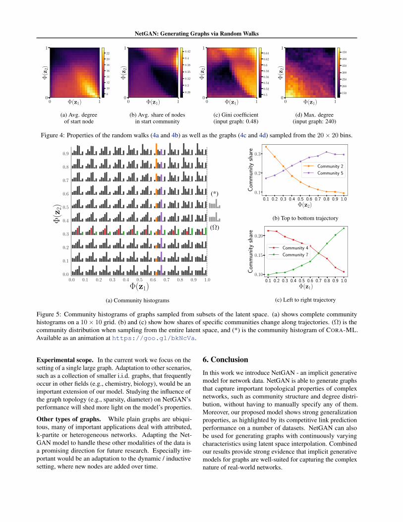
We can also see this mapping from latent space to the gen-erated graph properties in the community distribution his-tograms on a 10 × 10 grid in Fig. 5. Marked by (*) and(Ω) we see the community distributions for the input graphand the graph obtained by sampling on the complete latent

space respectively. In Fig. 5b and 5c, we see the evolutionof selected community shares when following a trajectoryfrom top to bottom, and left to right, respectively. The com-munity histograms resulting from sampling random walksfrom opposing regions of the latent space are very different;again the transitions between these histograms are smooth,as can be seen in the trajectories in Fig. 5b and 5c.

5. Discussion and Future WorkWhen evaluating different graph generative models in Sec.3.2, we observed a major limitation of explicit models.While the prescribed approaches excel at recovering theproperties directly included in their definition, they performsignificantly worse with respect to the rest. This clearlyindicates the need for implicit graph generators such asNetGAN. Indeed, we notice that our model is able to con-sistently capture all the important graph characteristics (seeTable 1). Moreover, NetGAN generalizes beyond the inputgraph, as can be seen by its strong link prediction perfor-mance in Sec. 4.2. Still, being the first model of its kind,NetGAN possesses certain limitations, and a number ofrelated questions could be addressed in follow-up works:

Scalability. We have observed in Sec. 4.2 that it takes alarge number of generated random walks to get represen-tative transition counts for large graphs. While samplingrandom walks from NetGAN is trivially parallelizable, apossible extension of our model is to use a conditional gen-erator, i.e. the generator can be provided a desired startingnode, thus ensuring a more even coverage. On the otherhand, the sampling procedure itself can be sped up by in-corporating a hierarchical softmax output layer - a methodcommonly used in natural language processing.

Evaluation. It is nearly impossible to judge whether agraph is realistic by visually inspecting it (unlike images,for example). In this work we already quantitatively evaluatethe performance of NetGAN on a large number of standardgraph statistics. However, developing new measures ap-plicable to (implicit) graph generative models will deepenour understanding of their behavior, and is an importantdirection for future work.


0 1Φ(z1)0

1Φ

(z2)

8

10

12

14

16

18

20

22

(a) Avg. degreeof start node

0 1Φ(z1)0

1

Φ(z

2)

0.28

0.3

0.32

0.35

0.38

0.4

0.42

(b) Avg. share of nodesin start community

0 1Φ(z1)0

1

Φ(z

2)

0.5

0.52

0.54

0.56

0.58

0.6

0.62

0.64

(c) Gini coefficient(input graph: 0.48)

0 1Φ(z1)0

1

Φ(z

2)

150

200

250

300

350

400

450

(d) Max. degree(input graph: 240)

Figure 4: Properties of the random walks (4a and 4b) as well as the graphs (4c and 4d) sampled from the 20× 20 bins.

0.0 0.1 0.2 0.3 0.4 0.5 0.6 0.7 0.8 0.9 1.00.0

0.1

0.2

0.3

0.4

0.5

0.6

0.7

0.8

0.9

Φ(z

2)

Φ(z1)

(Ω)

(*)

(a) Community histograms

0.1 0.2 0.3 0.4 0.5 0.6 0.7 0.8 0.9 1.0Φ(z2)

0.1

0.2

0.3

Com

mun

ity

shar

e

Community 2

Community 5

(b) Top to bottom trajectory

0.1 0.2 0.3 0.4 0.5 0.6 0.7 0.8 0.9 1.0Φ(z1)

0.10

0.15

0.20

Com

mun

ity

shar

eCommunity 4

Community 7

(c) Left to right trajectory

Figure 5: Community histograms of graphs sampled from subsets of the latent space. (a) shows complete communityhistograms on a 10× 10 grid. (b) and (c) show how shares of specific communities change along trajectories. (Ω) is thecommunity distribution when sampling from the entire latent space, and (*) is the community histogram of CORA-ML.Available as an animation at https://goo.gl/bkNcVa.

Experimental scope. In the current work we focus on thesetting of a single large graph. Adaptation to other scenarios,such as a collection of smaller i.i.d. graphs, that frequentlyoccur in other fields (e.g., chemistry, biology), would be animportant extension of our model. Studying the influence ofthe graph topology (e.g., sparsity, diameter) on NetGAN’sperformance will shed more light on the model’s properties.

Other types of graphs. While plain graphs are ubiqui-tous, many of important applications deal with attributed,k-partite or heterogeneous networks. Adapting the Net-GAN model to handle these other modalities of the data isa promising direction for future research. Especially im-portant would be an adaptation to the dynamic / inductivesetting, where new nodes are added over time.

6. ConclusionIn this work we introduce NetGAN - an implicit generativemodel for network data. NetGAN is able to generate graphsthat capture important topological properties of complexnetworks, such as community structure and degree distri-bution, without having to manually specify any of them.Moreover, our proposed model shows strong generalizationproperties, as highlighted by its competitive link predictionperformance on a number of datasets. NetGAN can alsobe used for generating graphs with continuously varyingcharacteristics using latent space interpolation. Combinedour results provide strong evidence that implicit generativemodels for graphs are well-suited for capturing the complexnature of real-world networks.

https://goo.gl/bkNcVa


AcknowledgmentsThis research was supported by the German Research Foun-dation, Emmy Noether grant GU 1409/2-1, and by the Tech-nical University of Munich - Institute for Advanced Study,funded by the German Excellence Initiative and the Euro-pean Union Seventh Framework Programme under grantagreement no 291763, co-funded by the European Union.

ReferencesAdamic, L. A. and Adar, E. Friends and neighbors on the

web. Social networks, 25(3):211–230, 2003.

Adamic, L. A. and Glance, N. The political blogosphere andthe 2004 US election: divided they blog. In Proceedingsof the international workshop on Link discovery, pp. 36–43, 2005.

Arjovsky, M., Chintala, S., and Bottou, L. WassersteinGAN. arXiv preprint arXiv:1701.07875, 2017.

Barabasi, A.-L. and Albert, R. Emergence of scaling inrandom networks. Science, 286(5439):509–512, 1999.

Bender, E. A. and Canfield, E. R. The asymptotic numberof labeled graphs with given degree sequences. Journalof Combinatorial Theory, Series A, 24(3):296–307, 1978.

Berthelot, D., Schumm, T., and Metz, L. Began: Bound-ary equilibrium generative adversarial networks. arXivpreprint arXiv:1703.10717, 2017.

Blanken, H. M., de Vries, A. P., Blok, H. E., and Feng, L.Multimedia retrieval. 2007.

Bojchevski, A. and Gunnemann, S. Bayesian robust at-tributed graph clustering: Joint learning of partial anoma-lies and group structure. In Proceedings of the AAAIConference on Artificial Intelligence, 2018, pp. 2738–2745.

Bojchevski, A. and Gunnemann, S. Deep gaussian em-bedding of graphs: Unsupervised inductive learning viaranking. In International Conference on Learning Repre-sentations, 2018.

Broido, A. D. and Clauset, A. Scale-free networks are rare.arXiv preprint arXiv:1801.03400, 2018.

Chakrabarti, D. and Faloutsos, C. Graph mining: Laws,generators, and algorithms. Computing Surveys (CSUR),38(1):2, 2006.

Che, T., Li, Y., Zhang, R., Hjelm, R. D., Li, W., Song,Y., and Bengio, Y. Maximum-likelihood augmented dis-crete generative adversarial networks. arXiv preprintarXiv:1702.07983, 2017.

Choi, E., Biswal, S., Malin, B., Duke, J., Stewart, W. F., andSun, J. Generating multi-label discrete electronic healthrecords using generative adversarial networks. arXivpreprint arXiv:1703.06490, 2017.

Dong, Y., Johnson, R. A., Xu, J., and Chawla, N. V. Struc-tural diversity and homophily: A study across more thanone hundred big networks. In Proceedings of the SIGKDDInternational Conference on Knowledge Discovery andData Mining, pp. 807–816, 2017.

Goldenberg, A., Zheng, A. X., Fienberg, S. E., Airoldi,E. M., et al. A survey of statistical network models.Foundations and Trends in Machine Learning, 2(2):129–233, 2010.

Goodfellow, I. NIPS 2016 tutorial: Generative adversarialnetworks. arXiv preprint arXiv:1701.00160, 2016.

Goodfellow, I., Pouget-Abadie, J., Mirza, M., Xu, B.,Warde-Farley, D., Ozair, S., Courville, A., and Bengio,Y. Generative adversarial nets. In Advances in neuralinformation processing systems, pp. 2672–2680, 2014.

Grover, A. and Leskovec, J. node2vec: Scalable featurelearning for networks. In Proceedings of the SIGKDDinternational conference on Knowledge discovery anddata mining, pp. 855–864, 2016.

Gulrajani, I., Ahmed, F., Arjovsky, M., Dumoulin, V., andCourville, A. Improved training of Wasserstein GANs.arXiv preprint arXiv:1704.00028, 2017.

Handcock, M. S., Hunter, D. R., Butts, C. T., Goodreau,S. M., Krivitsky, P. N., and Morris, M. ERGM: Fit, Sim-ulate and Diagnose Exponential-Family Models for Net-works. The Statnet Project, 2017. R package version3.8.0.

Hjelm, R. D., Jacob, A. P., Che, T., Cho, K., and Bengio, Y.Boundary-seeking generative adversarial networks. arXivpreprint arXiv:1702.08431, 2017.

Hochreiter, S. and Schmidhuber, J. Long short-term memory.Neural Computation, 9(8):1735–1780, 1997.

Holland, P. W. and Leinhardt, S. An exponential familyof probability distributions for directed graphs. Journalof the american Statistical association, 76(373):33–50,1981.

Jang, E., Gu, S., and Poole, B. Categorical repa-rameterization with Gumbel-softmax. arXiv preprintarXiv:1611.01144, 2016.

Karras, T., Aila, T., Laine, S., and Lehtinen, J. Progres-sive growing of gans for improved quality, stability, andvariation. arXiv preprint arXiv:1710.10196, 2017.


Karrer, B. and Newman, M. E. Stochastic blockmodels andcommunity structure in networks. Physical Review E, 83(1):016107, 2011.

Kim, M. and Leskovec, J. Modeling social networks withnode attributes using the multiplicative attribute graphmodel. arXiv preprint arXiv:1106.5053, 2011.

Kingma, D. and Ba, J. Adam: A method for stochasticoptimization. arXiv preprint arXiv:1412.6980, 2014.

Kipf, T. N. and Welling, M. Variational graph auto-encoders.arXiv preprint arXiv:1611.07308, 2016.

Kusner, M. J. and Hernandez-Lobato, J. M. GANs forsequences of discrete elements with the Gumbel-softmaxdistribution. arXiv preprint arXiv:1611.04051, 2016.

Li, J., Monroe, W., Shi, T., Ritter, A., and Jurafsky, D.Adversarial learning for neural dialogue generation. arXivpreprint arXiv:1701.06547, 2017.

Liang, X., Hu, Z., Zhang, H., Gan, C., and Xing, E. P. Recur-rent topic-transition GAN for visual paragraph generation.arXiv preprint arXiv:1703.07022, 2017.

Liu, W., Chen, P.-Y., Cooper, H., Oh, M. H., Yeung, S., andSuzumura, T. Can GAN learn topological features of agraph? arXiv preprint arXiv:1707.06197, 2017.

McCallum, A. K., Nigam, K., Rennie, J., and Seymore,K. Automating the construction of internet portals withmachine learning. Information Retrieval, 3(2):127–163,2000.

Molloy, M. and Reed, B. A critical point for random graphswith a given degree sequence. Random structures &algorithms, 6(2-3):161–180, 1995.

Pan, S., Wu, J., Zhu, X., Zhang, C., and Wang, Y. Tri-partydeep network representation. Network, 11(9):12, 2016.

Peixoto, T. P. The graph-tool python library. URLhttp://figshare.com/articles/graph_tool/1164194.

Perozzi, B., Al-Rfou, R., and Skiena, S. Deepwalk: On-line learning of social representations. In Proceedingsof the SIGKDD international conference on Knowledgediscovery and data mining, pp. 701–710, 2014.

Sen, P., Namata, G., Bilgic, M., Getoor, L., Galligher, B.,and Eliassi-Rad, T. Collective classification in networkdata. AI magazine, 29(3):93, 2008.

Seshadhri, C., Kolda, T. G., and Pinar, A. Communitystructure and scale-free collections of Erdos-Renyi graphs.Physical Review E, 85(5):056109, 2012.

Tavakoli, S., Hajibagheri, A., and Sukthankar, G. Learn-ing social graph topologies using generative adversarialneural networks. 2017.

Wang, H., Wang, J., Wang, J., Zhao, M., Zhang, W., Zhang,F., Xie, X., and Guo, M. GraphGAN: Graph represen-tation learning with generative adversarial nets. arXivpreprint arXiv:1711.08267, 2017.

Wu, J., Zhang, C., Xue, T., Freeman, B., and Tenenbaum,J. Learning a probabilistic latent space of object shapesvia 3d generative-adversarial modeling. In Advances inNeural Information Processing Systems, pp. 82–90, 2016.

Yu, L., Zhang, W., Wang, J., and Yu, Y. SeqGAN: Sequencegenerative adversarial nets with policy gradient. In AAAI,pp. 2852–2858, 2017.

http://figshare.com/articles/graph_tool/1164194

http://figshare.com/articles/graph_tool/1164194


A. Graph statistics

Table 4: Graph statistics used to measure graph properties in this work.Metric name Computation DescriptionMaximum degree max

v∈Vd(v) Maximum degree of all nodes in a graph.

Assortativity ρ = cov(X,Y )σXσY

Pearson correlation of degrees of connected nodes, where the (xi, yi)pairs are the degrees of connected nodes.

Triangle count |u,v,w|(u,v),(v,w),(u,w)⊆E|6

Number of triangles in the graph, where u ∼ v denotes that u and vare connected.

Power law exponent 1 + n

( ∑u∈V

log d(u)dmin

)−1 Exponent of the power law distribution, where dmin denotes the mini-mum degree in a network.

Inter-community density 1K

∑Kj=1

∑Kk=1k 6=j

1

(|Ck||Cj |

)

∑u∈Cj

∑v∈Ck

Auv Fraction of possible inter-community edges present in graph.

Intra-community density 1K

∑Kj=1

1

(|Cj |2 )

∑u,v∈Cj

Auv Fraction of possible intra-community edges present in graph.

Wedge count∑v∈V

(d(v)2

)Number of wedges (2-stars), i.e. two-hop paths in an undirected graph.

Rel. edge distr. entropy 1ln |V |

∑v∈V −

d(v)|E| ln d(v)

|E|Entropy of degree distribution, 1 means uniform, 0 means a singlenode is connected to all others.

LCC Nmax = maxf⊆F

|f | Size of largest connected component, where F are all connected com-ponents of the graph.

Claw count∑v∈V

(d(v)3

)Number of claws (3-stars)

Gini coefficient 2∑|V |

i=1 idi

|V |∑|V |

i=1 di− |V |+1

|V |Common measure for inequality in a distribution, where d is the sortedlist of degrees in the graph.

Community distribution ci =∑

v∈Cid(v)∑

v∈V d(v)

Share of in- and outgoing edges of community Ci, normalized by thenumber of edges in the graph.

B. Baselines• Configuration model. In addition to randomly rewiring all edges in the input graph, we also generate random graphs

with similar overlap as graphs generated by NetGAN using the configuration model. For this, we randomly select ashare of edges (e.g. 39%) and keep them fixed, and shuffle the remaining edges. This leads to a graph with the specifiededge overlap; in Table 2 we show that with the same edge overlap, NetGAN’s generated graphs in general match theinput graph better w.r.t the statistics we measure.

• Exponential random graph model. We use the R implementation of ERGM from the ergm package (Handcocket al., 2017). We used the following parameter settings: edge count, density, degree correlation,deg1.5, and gwesp. Here, deg1.5 is the sum of all degrees to the power of 1.5, and gwesp refers to thegeometrically weighted edgewise shared partner distribution.

• Degree-corrected stochastic blockmodel. We use the Python implementation from the graph-tool package(Peixoto) using the recommended hyperparameter settings.

• Variational graph autoencoder. We use the implementation provided by the authors (https://github.com/tkipf/gae). We construct the graph from the predicted edge probabilities using the same protocol as in Sec. 3.3 ofour paper. To ensure a fair comparison we perform early stopping, i.e. select the weights that achieve the best validationset performance.

https://github.com/tkipf/gae

https://github.com/tkipf/gae


C. Properties of generated graphs

Table 5: Comparison of graph statistics between the CITESEER/CORA-ML graph and graphs generated by GraphGAN andDC-SBM, averaged after 5 trials.

Graph Max.degree Assortativity Triangle

countPower lawexponent

Avg. Inter-com-munity density

Avg. Intra-com-munity density

Clusteringcoefficient

Avg. Std. Avg. Std. Avg. Std. Avg. Std. Avg. Std. Avg. Std. Avg. Std.CITESEER 77 -0.022 451 2.239 4.9e-4 9.3e-4 1.08e-2Conf. model * * -0.017± 0.006 20 ± 6.50 * * 1.1e-3± 1e-5 2.3e-4± 2e-5 5.80e-4± 1.29e-4Conf. model (42% EO) * * -0.020± 0.009 54 ± 8.8 * * 8.4e-4± 1e-5 5.1e-4± 1e-5 1.33e-3± 6.15e-5Conf. model (76% EO) * * -0.024± 0.006 207 ± 11.8 * * 6.3e-4± 1e-5 7.6e-4± 1e-5 5.00e-3± 2.57e-4DC-SBM (6.6% EO) 53 ± 5.6 0.022 ± 0.018 257 ± 30.9 2.066 ± 0.014 7.6e-4± 2e-5 5.3e-4± 3e-5 1.00e-2± 2.63e-3ERGM (27% EO) 66 ± 1 0.052 ± 0.005 415.6 ± 8 2.0 ± 0.01 9.3e-4± 2e-5 4.8e-4± 6e-6 1.49e-2± 5.68e-4BTER (2% EO) 70 ± 7.2 0.065 ± 0.014 449 ± 33 2.049 ± 0.01 1.1e-3± 2e-5 2.8e-4± 6e-6 1.22e-2± 2.31e-3VGAe (0.2% EO) 9.2 ± 0.7 -0.057± 0.016 2 ± 1 2.039 ± 0.00 1.2e-3± 1e-5 2.5e-4± 2e-5 1.35e-3± 9.96e-4NetGAN VAL (42% EO) 54 ± 4.2 -0.082± 0.009 316 ± 11.2 2.154 ± 0.003 6.5e-4± 2e-5 8.0e-4± 2e-5 1.99e-2± 3.48e-3NetGAN EO (76% EO) 63 ± 4.3 -0.054± 0.006 227 ± 13.3 2.204 ± 0.003 5.9e-4± 2e-5 8.6e-4± 1e-5 7.71e-3± 2.43e-4CORA-ML 240 -0.075 2,814 1.86 4.3e-4 1.7e-3 2.73e-3Conf. model * * -0.030± 0.003 322 ± 31 * * 1.6e-3± 1e-5 2.8e-4± 1e-5 3.00e-4± 2.88e-5Conf. model (39% EO) * * -0.050± 0.005 420 ± 14 * * 1.1e-3± 1e-5 8.0e-4± 1e-5 4.10e-4± 1.40e-5Conf. model (52% EO) * * -0.051± 0.002 626 ± 19 * * 9.8e-4± 1e-5 9.9e-4± 2e-5 6.10e-4± 1.85e-5DC-SBM (11% EO) 165 ± 9.0 -0.052± 0.004 1,403 ± 67 1.814 ± 0.008 6.7e-4± 2e-5 1.2e-3± 4e-5 3.30e-3± 2.71e-4ERGM (56% EO) 243 ± 1.94 -0.077± 0.000 2,293 ± 23 1.786 ± 0.003 6.9e-4± 2e-5 1.2e-3± 1e-5 2.17e-3± 5.44e-5BTER (2% EO) 199 ± 13 0.033 ± 0.008 3060 ± 114 1.787 ± 0.004 1.1e-3± 1e-5 7.5e-4± 1e-5 4.62e-3± 5.92e-4VGAe (0.3% EO) 13.1 ± 1 -0.010± 0.014 14 ± 3 1.674 ± 0.001 1.4e-3± 2e-5 3.2e-4± 1e-5 1.17e-3± 2.02e-4NetGAN VAL (39% EO) 199 ± 6.7 -0.060± 0.004 1,410 ± 30 1.773 ± 0.002 6.5e-4± 1e-5 1.3e-3± 2e-5 2.33e-3± 1.75e-4NetGAN EO (52% EO) 233 ± 3.6 -0.066± 0.003 1,588 ± 59 1.793 ± 0.003 6.0e-4± 1e-5 1.4e-3± 1e-5 2.44e-3± 1.91e-4

Graph Wedge count Rel. edgedistr. entr.

Largestconn. comp Claw count Gini coeff. Edge overlap Characteristic

path lengthAvg. Std. Avg. Std. Avg. Std. Avg. Std. Avg. Std. Avg. Std. Avg. Std.

CITESEER 16,824 0.959 2,110 125,701 0.404 1 10.33Conf. model * * 0.955 ± 0.001 2,011 ± 6.8 * * * * 0.008 ± 0.001 5.95 ± 0.03Conf. model (42% EO) * * 0.956 ± 0.001 2,045 ± 12.5 * * * * 0.42 ± 0.002 6.14 ± 0.03Conf. model (76% EO) * * 0.957 ± 0.001 2,065 ± 10.2 * * * * 0.76 ± 0.0 6.85 ± 0.04DC-SBM (6.6% EO) 15,531 ± 592 0.938 ± 0.001 1,697 ± 27 69,818 ± 11,969 0.502 ± 0.005 0.066 ± 0.011 7.75 ± 0.26ERGM (27% EO) 16,346 ± 101 0.945 ± 0.001 1,753 ± 15 80,510 ± 1,337 0.474 ± 0.003 0.27 ± 0.01 5.92 ± 0.01BTER (2% EO) 18,193 ± 661 0.940 ± 0.001 1,708 ± 14 113,425± 19,737 0.491 ± 0.007 0.02 ± 0.002 5.66 ± 0.07VGAe (0.2% EO) 8,141 ± 47 0.986 ± 0.000 2,110 ± 0 6,611 ± 144 0.256 ± 0.003 0.002 ± 0.001 7.75 ± 0.04NetGAN VAL (42% EO) 12,998 ± 84.6 0.969 ± 0.000 2,079 ± 12.6 57,654 ± 4,226 0.354 ± 0.001 0.42 ± 0.006 8.28 ± 0.11NetGAN EO (76% EO) 15,202 ± 378 0.963 ± 0.000 2,053 ± 23 94,149 ± 11,926 0.385 ± 0.002 0.76 ± 0.01 7.68 ± 0.13CORA-ML 101,872 0.941 2,810 3.1e6 0.482 1 5.61Conf. model * * 0.928 ± 0.002 2,785 ± 4.9 * * * * 0.013 ± 0.001 4.38 ± 0.01Conf. model (39% EO) * * 0.931 ± 0.002 2,793 ± 2.0 * * * * 0.39 ± 0.0 4.41 ± 0.02Conf. model (52% EO) * * 0.933 ± 0.001 2,793 ± 6.0 * * * * 0.52 ± 0.0 4.46 ± 0.02DC-SBM (11% EO) 73,921 ± 3,436 0.934 ± 0.001 2,474 ± 18.9 1.2e6 ± 170,045 0.523 ± 0.003 0.11 ± 0.003 5.12 ± 0.04ERGM (56% EO) 98,615 ± 385 0.932 ± 0.001 2,489 ± 11 3,1e6 ± 57,092 0.517 ± 0.002 0.56 ± 0.014 4.59 ± 0.02BTER (2% EO) 91,813 ± 3,546 0.935 ± 0.000 2,439 ± 19 2.0e6 ± 280,945 0.515 ± 0.003 0.02 ± 0.001 4.59 ± 0.03VGAe (0.3% EO) 31,290 ± 178 0.990 ± 0.000 2,810 ± 0 46,586 ± 937 0.223 ± 0.003 0.003 ± 0.001 5.28 ± 0.01NetGAN VAL (39% EO) 75,724 ± 1,401 0.959 ± 0.000 2,809 ± 1.6 1.8e6 ± 141,795 0.398 ± 0.002 0.39 ± 0.004 5.17 ± 0.04NetGAN EO (52% EO) 86,763 ± 1,096 0.954 ± 0.001 2,807 ± 1.6 2.6e6 ± 103,667 0.42 ± 0.003 0.52 ± 0.001 5.20 ± 0.02


D. Graph statistics during the training process


0k 20k 40k 60k 80k 100k

Training iteration

100

150

200

250

Max. degre

e

(a)

0k 20k 40k 60k 80k 100k

Training iteration

0.08

0.06

0.04

0.02

Ass

ort

ati

vit

y(b)

0k 20k 40k 60k 80k 100k

Training iteration

0

1000

2000

Tri

angle

count

(c)

0k 20k 40k 60k 80k 100k

Training iteration

1.775

1.800

1.825

1.850

Pow

er

law

exp.

(d)

0k 20k 40k 60k 80k 100k

Training iteration

2500

2600

2700

2800

LCC

(e)

0k 20k 40k 60k 80k 100k

Training iteration

0.00

0.25

0.50

0.75

1.00

Ed

ge

ov

erl

ap

(f)

Figure 7: Evolution of graph statistics during training on CORA-ML


0k 20k 40k 60k 80k 100k

Training iteration

40

50

60

70

Max. degre

e

(a)

0k 20k 40k 60k 80k 100k

Training iteration

0.075

0.050

0.025

0.000

Ass

ort

ati

vit

y

(b)

0k 20k 40k 60k 80k 100k

Training iteration

0

100

200

300

400

Tri

angle

count

(c)

0k 20k 40k 60k 80k 100k

Training iteration

2.10

2.15

2.20

Pow

er

law

exp.

(d)

0k 20k 40k 60k 80k 100k

Training iteration

1700

1800

1900

2000

2100

LCC

(e)

0k 20k 40k 60k 80k 100k

Training iteration

0.00

0.25

0.50

0.75

1.00

Edge o

verl

ap

(f)

Figure 8: Evolution of graph statistics during training on CITESEER


E. Latent space interpolation heatmaps

0 1Φ(z1)0

1

Φ(z

2)

8

10

12

14

16

18

20

22


0 1Φ(z1)0

1

Φ(z

2)

0.28

0.3

0.32

0.35

0.38

0.4

0.42

(b) Avg. share of nodes in thesame comm. as the starting node

0 1Φ(z1)0

1

Φ(z

2)

0.5

0.52

0.54

0.56

0.58

0.6

0.62

0.64


0 1Φ(z1)0

1

Φ(z

2)

150

200

250

300

350

400

450


0 1Φ(z1)0

1

Φ(z

2)

−0.1

−0.08

−0.06

−0.04

−0.02

0.0

(e) Assortativity(input graph: -0.075)

0 1Φ(z1)0

1

Φ(z

2)

14.75

15.0

15.25

15.5

15.75

16.0

16.25

16.5

16.75

(f) Claw count(input graph: 3.1× 106)

0 1Φ(z1)0

1

Φ(z

2)

0.88

0.89

0.9

0.91

0.92

0.93

(g) Rel. edge distr. entro-py (input graph: 0.94)

0 1Φ(z1)0

1

Φ(z

2)

2720

2740

2760

2780

2800

(h) Largest conn. comp.(input graph: 2,810)

0 1Φ(z1)0

1

Φ(z

2)

0.05

0.06

0.06

0.06

0.07

0.08

0.08

(i) Edgeoverlap

0 1Φ(z1)0

1

Φ(z

2)

2.25

2.5

2.75

3.0

3.25

3.5

3.75

4.0

4.25

(j) Power law exponent(input graph: 1.86)

0 1Φ(z1)0

1

Φ(z

2)

0.76

0.78

0.8

0.82

0.84

(k) Avg. precisionlink prediction

0 1Φ(z1)0

1

Φ(z

2)

0.66

0.68

0.7

0.72

0.74

0.76

(l) ROC AUClink prediction

0 1Φ(z1)0

1

Φ(z

2)

0.01

0.02

0.03

0.04

(m) Share of walksin single community

0 1Φ(z1)0

1

Φ(z

2)

0.88

0.9

0.92

0.94

0.96

(n) tAvg. start node entropy

0 1Φ(z1)0

1

Φ(z

2)

1000

2000

3000

4000

5000

(o) Triangle count(input graph: 2,814)

0 1Φ(z1)0

1

Φ(z

2)

120000

140000

160000

180000

200000

(p) Wedge count(input graph: 101,872)

Figure 9: Properties of the random walks as well as the graphs sampled from the 20 × 20 latent space bins, trained onCORA-ML.


0 1Φ(z1)0

1

Φ(z

2)

4

5

6

7

8

9


0 1Φ(z1)0

1

Φ(z

2)

0.4

0.42

0.44

0.46

0.48

0.5

(b) Avg. share of nodes in startcommunity

0 1Φ(z1)0

1

Φ(z

2)

0.38

0.4

0.42

0.44

0.46

0.48


0 1Φ(z1)0

1

Φ(z

2)

60

70

80

90

100

110

120

130

140


0 1Φ(z1)0

1

Φ(z

2)

−0.08

−0.06

−0.04

−0.02

0.0

(e) Assortativity(input graph: -0.022)

0 1Φ(z1)0

1

Φ(z

2)

11.5

12.0

12.5

13.0

13.5

(f) Claw count(input graph: 125,701)

0 1Φ(z1)0

1

Φ(z

2)

0.94

0.94

0.94

0.95

0.96

0.96

0.96

(g) Rel. edge distr. entro-py (input graph: 0.96)

0 1Φ(z1)0

1

Φ(z

2)

2050

2060

2070

2080

2090

2100

2110

(h) Largest conn. comp.(input graph: 2,110)

0 1Φ(z1)0

1

Φ(z

2)

0.12

0.12

0.12

0.13

0.14

0.14

0.14

0.15

0.16

(i) Edgeoverlap

0 1Φ(z1)0

1

Φ(z

2)

2.2

2.25

2.3

2.35

2.4

(j) Power law exponent(input graph: 2.239)

0 1Φ(z1)0

1

Φ(z

2)

0.9

0.91

0.92

0.93

0.94

0.95

0.96

(k) Avg. precisionlink prediction

0 1Φ(z1)0

1

Φ(z

2)

0.84

0.86

0.88

0.9

0.92

(l) ROC AUClink prediction

0 1Φ(z1)0

1

Φ(z

2)

0.04

0.05

0.06

0.07

0.08

(m) Share of walksin single community

0 1Φ(z1)0

1

Φ(z

2)

0.84

0.86

0.88

0.9

0.92

0.94

0.96

(n) Avg. start node entropy

0 1Φ(z1)0

1

Φ(z

2)

150

200

250

300

350

400

(o) Triangle count(input graph: 451)

0 1Φ(z1)0

1

Φ(z

2)

15000

20000

25000

30000

35000

(p) Wedge count(input graph: 16,824)

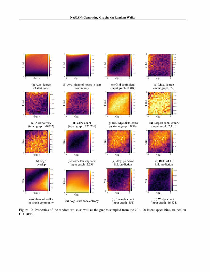
Figure 10: Properties of the random walks as well as the graphs sampled from the 20 × 20 latent space bins, trained onCITESEER.


F. Latent space interpolation community histrograms – CITESEER

0.0 0.1 0.2 0.3 0.4 0.5 0.6 0.7 0.8 0.9 1.0

0.0

0.1

0.2

0.3

0.4

0.5

0.6

0.7

0.8

0.9

Φ(z

2)

Φ(z1)

Figure 11: Community distributions of graphs generated by NetGAN on subregions of the latent space z, trained on theCITESEER network.

G. Recovering ground-truth edge probabilitiesTo further investigate the ability of NetGAN to capture the graph structure we perform an additional experiment with thegoal of analyzing how well we can recover the ground-truth edge probabilities given a graph generated from a prescribedgenerative model. Towards that end, first, we generate a graph from DC-SBM (N = 300 nodes and 3 communities), thenwe fit NetGAN on this graph, and finally we compare the ground truth edge probabilities to the edge scores inferred byNetGAN – specifically we compute their ranking correlation. We find a correlation of 0.998 (with EO = 0.42), which showsthat NetGAN uncovered the underlying generative process, without overfitting to the input graph.

H. Hyperparameter configurationAs discussed in Sec. 4.2 NetGAN is not sensitive to the choice of most hyperparameters. For completeness, we reporthere sensible defaults that we used in used in our experiments. The generator and discriminator each have a single hiddenlayer with 40 and 30 hidden units respectively. The down-projection matrix for the generator is W down,g ∈ RN×Hg withHg = 64, and for the discriminator is W down,d ∈ RN×Hd with Hd = 32. The latent code z is drawn from a d = 16dimensional multivariate standard normal distribution. We anneal the temperature from τ = 1.0 down to τ = 0.5 every 500iterations with a multiplicative decay of 0.995. We tune the parameters p and q (used to bias the generated random walks)for each dataset separately using the procedure in Grover & Leskovec (2016).We use Adam (Kingma & Ba, 2014) to optimize all the parameters with a learning rate of 1e−3 and we set the regularizationstrength for the L2 penalty to 1e−6. We perform five update steps for the parameters of the discriminator for each singleupdate step of the parameters of the generator, and we set the Wasserstein gradient penalty applied to the discriminator to 10as suggested by Gulrajani et al. (2017). For early stopping, we evaluate the score every 500 iterations, and set the patience to5 evaluation steps. To calculate the validation score we generate 15M transitions, e.g. for a random walk of length 16 (i.e.15 transitions per random walk) this equals 1M random walks.For more details we refer the reader to the provided reference implementation at https://www.kdd.in.tum.de/netgan.

https://www.kdd.in.tum.de/netgan

Documents

NetGAN: Generating Graphs via Random Walks · nary indicators, counts) in patient records. ... The goal of the generator is to generate synthetic random walks that are plausible in