NBER WORKING PAPER SERIES

INDIA’S DE-INDUSTRIALIZATION UNDER BRITISH RULE:NEW IDEAS, NEW EVIDENCE

David ClingingsmithJeffrey G. Williamson

Working Paper 10586http://www.nber.org/papers/w10586

NATIONAL BUREAU OF ECONOMIC RESEARCH1050 Massachusetts Avenue

Cambridge, MA 02138June 2004

Paper presented at the 5th World Congress of Cliometrics, Venice, July 8-11, 2004. We are grateful for adviceand criticism from Greg Clark, Ron Findlay, Bishnupriya Gupta, Leandro Prados, Debin Ma, Patrick O’Brien,Kevin O’Rourke, Sevket Pamuk, Ananth Seshadri, T. N. Srinivasan, Tony Venables, and participants in theHarvard Economic History Tea. We also thank Javier Cuenca Esteban for sharing his data. Williamsonacknowledges with pleasure financial support from the National Science Foundation SES-0001362, and thework environment at the University of Wisconsin Economics Department, where much of this paper waswritten while he was on leave from Harvard. The views expressed herein are those of the author(s) and notnecessarily those of the National Bureau of Economic Research.

©2004 by David Clingingsmith and Jeffrey G. Williamson. All rights reserved. Short sections of text, notto exceed two paragraphs, may be quoted without explicit permission provided that full credit, including ©notice, is given to the source.

India’s De-Industrialization Under British Rule: New Ideas, New EvidenceDavid Clingingsmith and Jeffrey G. WilliamsonNBER Working Paper No. 10586June 2004JEL No. F1, N7, O2

ABSTRACT

India was a major player in the world export market for textiles in the early 18th century, but by the

middle of the 19th century it had lost all of its export market and much of its domestic market. Other

local industries also suffered some decline, and India underwent secular de-industrialization as a

consequence. While India produced about 25 percent of world industrial output in 1750, this figure

fell to only 2 percent by 1900. We use an open, specific-factor model to organize our thinking about

the relative role played by domestic and foreign forces in India’s de-industrialization. The

construction of new relative price evidence is central to our analysis. We document trends in the

ratio of export to import prices (the external terms of trade) from 1800 to 1913, and that of tradable

to non-tradable goods and own-wages in the tradable sectors going back to 1765. With this new

relative price evidence in hand, we ask how much of the de-industrialization was due to local

supply-side influences (such as the demise of the Mughal empire) and how much to world price

shocks (such as world market integration and rapid productivity advance in European

manufacturing), both of which had to deal with an offset n the huge net transfer from India to

Britain before 1815. Whether the Indian de-industrialization shocks and responses were big or small

is then assessed by comparisons with other parts of the periphery.

David ClingingsmithDepartment of EconomicsHarvard UniversityCambridge, MA 02138clinging@fas.harvard.edu

Jeffrey G. WilliamsonDepartment of EconomicsHarvard UniversityCambridge, MA 02138and NBERjwilliam@kuznets.fas.harvard.edu

1

1. Introduction

The idea that India suffered de-industrialization during the 19th century has a long pedigree in the

historiography of the subcontinent. Its longevity seems to be due equally to powerful images of skilled artisans

thrown back on the soil and to the possibility that it offers an explanation of persistent Indian poverty. It also

was a potent weapon in the Indian nationalists’ critique of colonial rule. While de-industrialization is invoked

by just about every major anti-colonial historian of India, very few have made an attempt to assess empirically

whether and when it happened, what caused it, and whether it was more or less dramatic than elsewhere in the

periphery. This paper offers such an assessment. Our main contribution to the de-industrialization debate will

be newly compiled evidence on relative prices. The existing literature, to the extent it engages in quantitative

assessments at all, relies instead on changes in employment shares.

Definitions and a Theoretical Framework

How do we define de-industrialization? Consider the following simple framework. Suppose a

economy produces two commodities: agricultural goods, which are exported, and manufactured goods, which

are imported. It uses three factors of production: labor, which is mobile between the two sectors; land, which is

used only in agriculture; and capital, which is used only in manufacturing. Further suppose that this economy

is what trade economists call a “small country” that takes its terms of trade as exogenous, dictated by world

markets. Given these assumptions we define de-industrialization as the movement of labor out of

manufacturing and in to agriculture, either measured as a share in total employment (a weak de-

industrialization measure), or in absolute numbers (a strong de-industrialization measure). While de-

industrialization is easy enough to define in this simple 2x3 model, an assessment of its short and long run

impact on living standards and GDP growth is more contentious and hinges on the root causes of de-

industrialization.

One possibility is that a country de-industrializes because its comparative advantage in the agricultural

export sector has been strengthened either by productivity advance on the land at home or by increasing

openness in the world economy, or both. Under this scenario, GDP increases in the short-run. In the first case,

2

and still retaining the small country assumption, nothing happens to the terms of trade. However, if the small

country assumption is violated, then the country suffers a terms of trade deterioration, in that it has to share

part of the productivity increase in the agricultural export sector with its trading partners. In the second case,

the country enjoys an unambiguous terms of trade improvement as declining world trade barriers raise export

prices and lower import prices in the home market.

Whether real wages and the living standards of landless labor also increase depends on the direction of

the terms of trade change and whether the agricultural good dominates the worker’s budget. Whether GDP

increases in the long run depends on whether industry generates accumulation and productivity externalities

that agriculture does not. If industrialization is a carrier of growth – as most growth theories imply, then de-

industrialization could lead to a growth slowdown and a low-income equilibrium that gives the idea of de-

industrialization its power in the historical literature.

A second possibility is that a country de-industrializes due to a deterioration in home manufacturing

productivity and/or competitiveness. In this case, and still retaining the small country assumption, nothing

happens to the terms of trade, but real wages and living standards will deteriorate, and so will GDP. The

economic impact of de-industrialization from this source is unambiguous.

Explaining the Indian Experience

Which historical narrative works best in accounting for India’s de-industrialization experience over

the century and a half after 1750? Did the terms of trade rise, fall or remain unchanged? While the Indian de-

industrialization literature rarely checks its predictions against terms of trade and relative price experience, it

does have two contending hypotheses. One theorizes that de-industrialization was driven by the demise of the

Mughal empire, which caused supply-side problems in home manufacturing. The other suggests the driver was

the British victory in foreign markets for cottage-made manufactures, followed later by its penetration of the

Indian home market with cheap factory-produced manufactures. In other words, India suffered negative

globalization price shocks in its key manufacturing tradable. The latter theme is dominant among Indian

historians (Roy 2002). This paper takes the view that these hypotheses are complementary. To make them

more compatible, we have to replace two-sector thinking with three-sector thinking by adding a nontradeable

3

grain sector. The three sectors we will consider in the rest of the paper are: exportables, which include

industrial intermediates (such as raw cotton and jute) and exotic consumer goods (such as opium and tea);

importables, which are primarily textiles and metal products; and non-tradables, which include rice, wheat and

other grains. The overall de-industrialization argument is consistent with the following narrative that owes

much to Joseph Inikori (2002: Chp. 9) and Irfan Habib (1975, 1985).

The decline of the Mughal empire stretched over a long period, and the political and economic

stability it had provided reached a low ebb in the middle of the 18th century. The decline had a negative impact

on productivity in agriculture, which must have served to raise the price of the key non-tradable (grain) relative

to tradables (such as textiles).1 To the extent that grain was the dominant consumption good for workers, and if

the grain wage was close to subsistence, this negative productivity shock should have put upward pressure on

the nominal wage in cotton hand spinning and weaving, wages that started from a low nominal but high real

base in the mid-18th century (Parthasarathi 1998; Allen 2001). If this rise in the “own” wage in textiles was

big enough, it should have taken away much or all of the competitive edge India had in third-country export

markets, that is in the booming Atlantic economy. Radhakamal Mukerjee (1939) documented a spectacular

drop in Indian real wages 1650-1816 (Figure 1), but he was interested in living standards and thus divided

nominal wages by non-tradable grain prices. Instead, we are interested in the own (real) wage in manufacturing

generally, and textiles in particular, so we will divide the nominal wage by the (declining) cotton textile price.

Any rise in the own wage facing Indian textiles would have diminished its competitive edge in world markets.

Perhaps for this reason, then, during the mid-late 18th century Britain was already beginning to wrest away

India's long-standing leadership in the fastest growing world markets, West Africa and the Americas, where

cheap calicos were clothing the booming slave labor force, and Europe.2 So, even before factory-driven

1 We assume that India was a price taker for textiles and other manufactures. Given this assumption, domestic demand did not matter in determining the performance of Indian industry. Only price and competitiveness on the supply side mattered. Thus, we ignore as irrelevant any argument which appeals to a rise in the demand for cloth as per capita income rose (Harnetty 1991: 455, 506; Morris 1983: 669). 2 English merchants and English ships were the main suppliers to the Atlantic trade, a lot of it the so-called re-export trade. The share of Indian textiles in the West African trade was about 38 percent in the 1730s, 22 percent in the 1780s and 3 percent in the 1840s (Inikori 2002: 512-3 and 516). By the end of the 17th century, Indian calicos were a major force in European markets (Landes 1998: 154). For example, the share of Indian textiles in total English trade with southern Europe was more than 20 percent in the 1720s, but this share fell to about 6 percent in the 1780s and less than 4 percent in the 1840s (Inikori 2002: 517). India was losing its world market share in textiles during the 18th century, long before the industrial revolution.

4

technologies appeared sometime between 1780 and 1820, India was losing its previously-dominant grip on the

world export market for textiles.3

Indian employment and output de-industrialization effects are hard to see before 1810 since textile

exports were a relatively small share of total Indian textile production. They are also hard to see since between

1772 and 1815 there was a huge net financial transfer from India to Britain. The “drain resulting from contact

with the West was the excess of exports from India for which there was no equivalent import” (Furber 1948:

304), including “a bewildering variety of cotton goods for re-export or domestic [consumption], and the

superior grade of saltpeter that gave British cannon an edge” (Cuenca Esteban 2001: 65). Javier Cuenca

Esteban estimates these net financial transfers from India to Britain to have been (£000, per annum): 1772-

1775 403; 1776-1783 499; 1784-1792 1014; 1793-1802 261; 1803-1807 -58; 1808-1815 477; and 1816-1820 -

77 (Cuenca Esteban 2001: Table 1, line 20). At their peak in 1784-1792, these net Indian transfers still

amounted to less than 2 percent of British industrial output (Deane and Cole 1967: Table 37, 166, using 1801

“manufacture, mining, building”). As a share of Indian industrial output, these net transfers were probably

about the same.4 Thus, while a secular fall in the “drain” after the 1784-1792 peak must have served to speed

up de-industrialization in early 19th century India, the effect could not have been big. There were other

fundamentals that mattered far more.

After the French Wars, British factory-made yarn and cloth took away the local market from India,

and we finally see the impact of de-industrialization, c1810-c1850, an impact induced by positive terms of

trade shocks favoring India. Furthermore, the net “drain” from India was no longer present as an offset to the

underlying fundamentals. The long run sources of the de-industrialization were not just the post-1810

globalization price shocks, but were also the negative productivity shocks to agriculture induced by the earlier

3 To make matters worse, India, which had captured a good share of the English market in the 17th century, had -- as an English defensive response -- already been legislated out of that market by Parliamentary decree between 1701 and 1722 (Inikori 2002: 431-2), thus protecting local textile producers. But Parliament kept the Atlantic economy as a competitive free trade zone. Of course, the large Indian Ocean market was also a free trade zone, and India had dominated this for centuries (Chaudhuri 1978; Landes 1998: 154). 4 Maddison (2001: 184 and 214) estimates that in 1820 the GDP of the India (including present-day Bangladesh and Pakistan) was about three times that of the United Kingdom, but the industrial share must have been a lot smaller in India. The text assumes that these offsetting forces were roughly comparable.

5

Mughal decline.5 We do not see these hypothesized home and foreign effects as competing. They were both at

work, and they reinforced each other.

Do Indian relative price time series support this narrative? Section 4 will reconstruct three price series

– commodity agricultural exports (Pc), manufactured textiles (Pt) and non-tradable grains (Pg), three terms of

trade series – Pc/Pt, Pc/Pg and Pt/Pg, three wage series – the grain wage, the own-wage in the import

competing sector, and the own-wage in the export sector, plus an assessment of the evidence. Section 5 will

compare Indian de-industrializing terms of trade shocks with those from other parts of the periphery. As a

prelude to the data, the tests, and the comparisons, the next section offers a brief survey of the Indian de-

industrialization debate, and Section 3 presents a simple general equilibrium model of de-industrialization to

formalize predictions.

2. The Debate and Existing Evidence about Indian De-Industrialization

The Idea of India’s De-Industrialization

The first widely known report of Indian de-industrialization seems to have come from Sir William

Bentinck, Governor-General of India from 1833 to 1835, whose powerful and enduring image of the effect of

British mill cloth on the Indian cotton industry was quoted by Karl Marx in Das Kapital: “The misery hardly

finds a parallel in the history of commerce. The bones of the cotton-weavers are bleaching the plains of India”

(1977[1867], vol. 1: 558). Somewhat later, in the New York Daily Tribune, Marx referred to “the British

intruder who broke up the Indian handloom” (Harnetty 1991: 455).

De-industrialization first became an important theme in Indian historical writing during the early

period of the nationalist movement that sought increased control of the governance of India for Indians. The

nationalists agitated for representation in government, and an important part of their argument was that British

rule had failed India. The decline of indigenous industry was part of this failure. The nationalists argued that

competition with cheap British mill cloth drove Indians out of the handloom industry and into agriculture. A

5 Peter Harnetty would appear to agree, although he was speaking of the Central Provinces in the 1860s, after our century of interest starting roughly with 1750. Harnetty says (1991: 460): “The combination of high food prices and cheap cloth

6

few contended that this shift was an inevitable result of the cost advantages of British mechanized cotton

spinning and weaving, while most pointed to low tariffs on British imports,6 implicitly suggesting that

protection might have promoted the development of an indigenous mill industry.

While the economic effects of de-industrialization are buried in the distant 18th and 19th century past,

its potency as a political symbol dates from the first half of the 20th century, a symbol that helped push Indian

toward policies of economic isolation and protectionism. De-industrialization entered the historical literature

about the same time with the appearance of R. C. Dutt’s seminal 1906 work Economic History of India. It was

also a theme in the writing of prominent nationalist historians such as Dadabhai Naoroji and Jawaharlal Nehru,

and Marxists such as D. D. Kosambi. Nehru’s classic Discovery of India (1947) argued that India became

progressively ruralized in the 19th century owing to the destruction of artisanal employment, and that the

appalling poverty of the Indian people was of recent origin, and that both were attributable to colonial anti-

industrial policy (Nehru 1947: 247-53). That is, while autonomous parts of the periphery were able to raise

tariffs to help defend themselves against the flood of cheap European manufactures, colonial India was not

able to do so, forced as it was to maintain free trade. 7

The Two Supporting Hypotheses

The Mughal Demise Hypotheses: We are not the first to exploit the connection between labor

productivity in pre-industrial agriculture, nominal wages in manufacturing, and the resulting competitiveness

in world markets for manufactures. Alexander Gerschenkron (1962) and W. Arthur Lewis (1978: chp. 2) have

both used the argument to good effect in explaining why low productivity in agriculture helps explain the

absence or delay of industrial revolutions. More recently, Prasannan Parthasarathi (1998) has argued that while

low nominal wages in pre-colonial and early colonial India gave it the edge in world textile markets, living

standards for landless labor in the south of India were just as high as that in the south of England. Indian

productivity was higher in grain production, and thus grain prices were lower. A generation before

imports had a depressing effect on the local industry.” 6 Indian tariffs in 1885 were about the lowest in the periphery, averaging 3 percent, compared with about 30 percent in Latin America and the United States, about 17 percent in eastern Europe and the rest of the newly settled European offshoots (Williamson 2004).

7

Parthasarathi, this view was supported by Tapan Raychaudhuri in the Cambridge Economic History of India

(Raychaudhuri 1983: 5-6, 16-18, 32). What high productivity in Mughal agriculture gave, the demise of the

Mughal empire took away.

There seems to be plenty of evidence of economic decay in India across the 18th century, and given the

huge size of agriculture in all pre-industrial societies,8 the decay must have had its main source there. Since we

take grain to have been non-tradable internationally, any secular tendency for domestic demand to outpace

domestic supply would have raised grain prices. Was there an exogenous acceleration of population growth

that would have lowered labor productivity on the land, reduced food supply relative to demand, and thus

raised the price of food? Apparently not: population grew at only 0.26 percent per annum between 1700 and

1820, and this was only a trivial increase over what preceded it (Moosvi 2000: 322). Was there some other

negative shock to agricultural productivity and food supplies? Apparently so:

“At its height the Mughal empire had imposed on the greater part of the Indian sub-continent a fair

measure of political unity. Centralized administration, a uniform revenue policy, a network of inland

trade fostered by Mughal peace and active encouragement to an expanding overseas commerce

created [prosperity] … By the middle years of the eighteenth century the empire lay in ruins … The

imperial governors did not formally deny their allegiance to Delhi, but one after another they had

asserted their autonomy” (Raychaudhuri 1983: 3).

A weak and crumbling empire invited invasion from without and war within. All of this is well known.

Furthermore,

“Historians of a later generation have equated the decline of the Mughal empire with sharp downward

trends in the Indian economy, and assumed that by the mid-eighteenth century it had reached its

lowest ebb. In many parts of the empire for varying lengths of time, war and anarchy did produce dire

economic results” (Raychaudhuri 1983: 5).

And it was inevitable that the dire economic results would fall on agriculture, for centuries the source of a vast

surplus that made Indian rulers even richer than Louis XIVth (by a factor of ten! Landes (1998): 156).

7 Nehru particularly blamed the lack of effort by the colonial government to establish a mechanized textile industry in India. He also believed that repatriated Bengal land rent was a significant catalyst to the British industrial revolution.

8

Labor productivity in agriculture underwent a decline as the empire underwent decline. The

economics is familiar to development economists, economic historians and observers of modern agrarian

backwardness. The effective rent burden was raised by rapacious revenue farmers: “Production suffered from

these extreme extractions, and [as a result, grain] prices increased by 30 percent or more in the 1740s and

1750s” (Raychaudhuri 1983: 6). Revenue farming had always been present in India, and even the Mughal

rulers were unable to erase it entirely, but by the mid-18th century its resurgence had served to raise the

effective rent share to at least half: “With revenue assessment geared to 50 per cent or more, in contrast to

China’s 5 to 6 per cent, the Indian peasant had little incentive to invest labour or capital” (Raychaudhuri 1983:

17). To make matters worse, war, political instability and potential expropriation raised uncertainty and further

suppressed incentive to accumulate or innovate:

“It was not that the peasants were unaware of the possibilities of improvement or psychologically

averse to innovation. But in their new situation they could not take any risk [or make any investment]

until the profitability of new techniques or implements [or cattle] was demonstrated [and returned to

the peasant] …” (Raychaudhuri 1983: 170).

In addition, war and internal tolls must have suppressed regional trade and specialization within the sub-

continent. Thus, districts that had specialized in textiles and other manufactures, and had satisfied their excess

food requirements by grain imports from surplus districts, must have found the price of grains rising for

additional reasons.

The demise of the Mughal empire created “a scarcity of grains in all parts, [and] the wages of labour

[were] greatly enhanced” (Holwell 1766-1767, cited in Raychaudhuri 1983: 6). This presumed rise in nominal

wages would have slowly eroded the long-standing source of Indian 17th and 18th century competitiveness in

foreign textile markets, long before Britain flooded those markets with factory-made products, and declining

agricultural productivity in India must have been at the heart of it. After 1800, Indian “textile exports … could

not withstand the competition of English factory-produced cottons in the world market” (Habib 2002: 341).

The Globalization-Shock Hypothesis: The more popular of the two hypotheses being considered

here is the one associated with what economists would now call globalization shocks. Namely, rapid

8 Agriculture employed 68 percent of the Indian labor force even as late as 1901 (Roy 2002: 113).

9

productivity advance in European manufacturing – led by Britain – lowered the relative price of textiles, metal

products and other manufactures in world markets. The European industrial leaders shared those productivity

gains with the rest of the world as augmented world supplies of manufactures lowered world prices. The

relative price impact of that unbalanced productivity performance is illustrated best by trends in Britain’s terms

of trade which, according to Albert Imlah, fell by 40 percent over the four decades between 1801-1810 and

1841-1850 (Mitchell and Deane 1962: 331). That is, the price of British exports (manufactures) fell

dramatically compared with that of its imports (industrial intermediates, food and other primary products).

India’s textile producers – already well integrated into the world textile market -- faced a big negative price

shock on that score alone. Failing to keep up the factory-based productivity growth achieved abroad, the Indian

textile industry took the price hit, became less profitable and contracted. De-industrialization ensued. As if this

were not enough, the foreign-productivity-induced negative price shock was reinforced by another powerful

global event. Due to the decline of trade barriers between India and her foreign markets, especially Britain and

especially that induced by the transport revolution (Shah Mohammed and Williamson 2004), the relative

supply price of manufactures in India was driven down still further, and it was driven down even more

compared with Indian exports, since overseas transport improvements served to raise export prices in the home

market. These world market integration trends were induced by transport revolutions, and these served to

create “Dutch disease” effects in India: the import-competing sectors slumped, the export sectors boomed, and

de-industrialization was reinforced. Having defeated India in export markets by 1800, “after 1813 Lancashire

invaded India as well” (Habib 2002: 341).

The Measurement of Indian De-Industrialization: Inputs and Outputs

While de-industrialization is an important theme in Indian historiography, there appear to have been

only four attempts to directly measure the 19th century experience, all looking at employment. No relative price

evidence has yet been offered in the literature and no evidence yet covers the 18th century, a gap we attempt to

bridge in section 4. Tirthankar Roy (2000) offers a useful survey of the existing evidence, starting with this big

fact: It seems likely that the share of the work force engaged in industry was quite a bit higher in 1800

(probably 15-18 percent) than it was in 1900 (about 10 percent). In the strictest sense, therefore, long run de-

10

industrialization certainly did take place. However, the literature insists on some qualifications to this big de-

industrialization fact. First, many workers who gave up industry over the century were working only part-time.

Second, the import of machine-made goods only helps explain the demise of textiles. Third, while there was a

fall in textile employment, there was a rise in employment in indigo, opium, and saltpeter. Fourth, cheaper

imported cloth would have benefited consumers. Finally, the literature argues that cheaper imported yarn

would have reduced the production costs facing handloom weavers thus making them more competitive. All of

these qualifications make good sense except the last since cheaper European-factory-produced yarn would

have lowered the production costs not just for Indian handloom weavers but for weavers the world around,

including those tending looms in British factories. Thus, it is not at all clear how this made Indian weavers

more competitive with imported cloth.

The first evidence supporting the big de-industrialization fact was offered more than a half century

ago by Colin Clark (1950). Clark published tabulations of the 1881 and 1911 Census of India showing that the

share of the Indian workforce in manufacturing, mining, and construction declined from 28.4 to 12.4 percent

from 1881 to 1911, implying dramatic de-industrialization in the late 19th century. Daniel Thorner (1962) re-

examined the Census data and convincingly argued that the tabulations used by Clark were misleading. His

revised estimates show that the sectoral employment structure was stationary after 1901, with only a very small

decline in male non-agricultural employment between 1881 and 1901. Thorner used these revisions to make

two important points: first, if there was a major shift out of industry and into agriculture, it occurred before

1881, not after; and second, if de-industrialization occurred after 1881, it did so on a very modest scale, and all

of it took place before 1901.

The third attempt to measure de-industrialization looks to the early 19th century, closer to the years

which anecdotal evidence has always suggested were those of most dramatic de-industrialization. Amiya

Bagchi (1976a, b) has examined evidence collected between 1809 and 1813 by the East India Company

surveyor Buchanan Hamilton on handloom spinning and other traditional industry in Gangetic Bihar, an area

of eastern India. Bagchi compared Hamilton’s data with the 1901 Census estimates of the population

dependent on industry for the same area. His findings are presented in Table 1. The population dependent on

industrial employment requires an estimate of family size, and Bagchi makes two estimates using altenative

11

assumptions. He also removes commercial workers from the 1901 data to make them consistent with the 1809-

13 data. Spinners in Gangetic Bihar were almost exclusively women who spun in the afternoons (Dutt 1960:

232-5). Hamilton’s estimates show women earned about Rs. 3.25 annually at spinning, while a male day

laborer who worked 200 days would earn about Rs. 8 annually, all of which suggests that Assumption B is

more likely to be true. In either case, Bagchi’s evidence suggests a substantial decline in the industrial

employment share during the 19th century. When the Bagchi and Thorner evidence is combined, it suggests

that most of that substantial de-industrialization took place in the first half of the century.

While the employment share in “other industrial” occupations fell over the century as well, it is

important to note that a large share of this de-industrialization had its source in the decline of cotton spinning.9

If we rearrange Bagchi’s numbers a bit, the contribution of cotton spinning to overall de-industrialization is

much more transparent, as Table 2 makes clear. Since cotton spinning was performed part-time by women at

home using extremely simple technology, it may seem implausible to argue that the demise of cotton spinning

in the early 19th century destroyed India’s platform for modern industrialization. Yet British economic

historians assign the same importance to home-based cotton spinning: 17th and 18th century “proto-industrial”

cottage industries are said to have supplied the platform for the factory-based British industrial revolution that

followed in the late 18th century (Mokyr 1993: chps. 1-3). Furthermore, employment of women and children

was central to the process then too (Mokyr 1993: chp. 1; De Vries 1994).

Finally, in an unpublished study reported by Irfan Habib (1985), Amalendu Guha calculated the

amount of cotton yarn available for handloom production by subtracting the quantity used in local machine

production from total local yarn production and imports. The result documents a huge decline in yarn used for

handloom production, from 419 million pounds in 1850, to 240 in 1870 and to 221 in 1900. This indirect

evidence suggests that the decline in hand spinning documented for Gangetic Bihar in the early 19th century

was widespread, that it was followed by a decline in hand weaving during the mid-century, and that the decline

of both hand spinning and weaving was almost complete by 1870.

These facts are consistent with Peter Harnetty’s summary characterization of Indian handloom

weaving in the 19th century:

12

“At the opening of the century, the handloom weavers had supplied all the textile requirements of the

country and had maintained a flourishing export trade, notably to Britain [e.g. re-exports]. This

reached its peak in value in 1800 and in volume in 1802, thereafter, imports of Indian piece goods to

Britain declined sharply in face of competition from the growing British cotton industry.” “From

about 1840 … British imports entered the [local] market in strength.” “At the turn of the [19th]

century, India was absorbing more than 40 per cent of total British cloth exports to the world”

(Harnetty 1991: 472).

Actually, and to repeat, the trouble started over the half century before the 1800 peak with the challenge to

India’s dominant presence in foreign markets.

In 1982, Paul Bairoch used evidence similar to that reviewed above to assess de-industrialization not

only in India, but across the non-European periphery. Table 3 reports Bairoch’s survey as it was retold by

Colin Simmons (1985). In 1750, China and India combined to account for almost 57 percent of world

manufacturing output, while India itself accounted for almost a quarter. By 1800, India’s world share had

already eroded to less than a fifth, by 1860 to less than a tenth, and by 1880 the figure was less than 3 percent.

This point is worth stressing: India’s share in world manufacturing output declined precipitously in the half

century 1750-1800, before factory-led industrialization took hold in Britain. Note also that India’s experience

was often different than that of China or the rest of the periphery: Between 1750 and 1830 the Indian world

manufacturing output share dropped by 6.9 percentage points, much bigger than the fall elsewhere (China lost

a still significant 3 percentage points, and the rest of the periphery lost 2.6 percentage points). Bairoch’s data

suggest unambiguously that during the century before 1830, well before European factories flooded world

markets with manufactures, India suffered much more pronounced de-industrialization than did the rest of the

periphery. There must have been special conditions in India, such as the decline of the Mughals, that explain

this fact.

We have been citing Bairoch’s world output shares for the periphery, but these could have been driven

by fast growth abroad as well as slow growth at home. As we noted earlier, the economic implications of faster

growth abroad are much more benign than that of slow growth at home. Anticipating this criticism, Bairoch

9 The percent of industrial workers who were spinners fell from 82 to 15 between 1809-13 and 1901.

13

(1982: Tables 6 and 9) also documented that per capita levels of industrialization in India fell from an index of

7 in 1750, to 6 in 1830 and to 2 in 1880. Once again, since India’s export share of total manufacturing output

was small in 1750, the loss of its export trade does not show up as dramatic de-industrialization 1750-1830, but

when Europe penetrates local markets after 1830, it certainly does.

Real Wages and Indian De-industrialization

Models of de-industrialization such as that of Paul Krugman and Anthony Venables (1995) suggest

that de-industrialization should be accompanied by a long run decline in real wages. The evidence for 18th and

19th century India is not yet of high quality, but what we do have certainly documents secular deterioration.

Parthasarathi (1998) argues that real wages in mid-late 18th century South India were comparable to

those in the south of England, and thus that the rising living standard gap between the two was a late 18th and

19th century phenomenon. Robert Allen (2001) uses Mughal manuscript sources to compute the real wage in

1595 Agra, then the capital of the Mughal empire, and compares it to that of 1961, based on a common market

basket of consumer goods. Allen’s evidence documents a fall in the real wage by about 23 percent over those

366 years, and if Parthasarathi is correct, most of that fall must have taken place in the last 166 years.

Anthropometric evidence on south Indian indentured workers confirms the view that living standards stagnated

during the last half of the 19th century (Brannan et al. 1994). But perhaps the most telling evidence of real

wage performance, and its timing, comes from Mukerjee (1939: 54), reproduced in Figure 1. Mukerjee reports

1600-1938 real wages in northern India of unskilled and skilled labor (nominal wage rates, deflated by a food

market basket that includes barley, wheat, jowar, bajra and gram) starting with the same Ain-i-Akbari

benchmark used by Allen. Mukerjee documents a much bigger secular decline for the real wage of unskilled

labor, about 51 percent, than does Allen, about 23 percent, but the former offers useful information about

timing that the latter does not. According to Mukerjee, by 1850 unskilled real wages had already fallen by 48

of the total 51 percentage point fall which took place between 1600 and 1938. Indeed, they had already fallen

by 30 percentage points by 1807, three-fifths of the total.

Thus, it appears that real wages and living standards fell across the 18th and 19th centuries.

Furthermore, the vast majority of the real wage fall took place before1850, or even before 1807, not after. Was

14

de-industrialization responsible for the fall, and were the de-industrialization forces more powerful before

1850, or even before 1807, than after?

3. A Model of De-Industrialization

In order to formalize our intuition about the relationship between relative prices and de-

industrialization, we develop a 3x4 specific-factors model that relies on the classic contribution of Ronald

Jones (1971). Consider a perfectly competitive economy in which there are three sectors: textiles (T), grain

(G), and commodity exports (C). Commodity exports are nonfood items such as opium, tea, indigo, jute, and

raw cotton. Labor (L) is mobile between all three sectors, and each sector also uses a specific factor: textiles

use capital (K, with return r), grains use grain-specific land (RG, with return dG), and commodity production

uses commodity-specific land (RC, with return dC). We justify the sector-specific land assumption by noting

that export commodities like jute, cotton and tea were usually produced on large farms or plantations, and in

quite specific climate zones. Grains were usually produced on small plots, and land transfer between crops was

very imperfect. Commodity prices are denoted pT, pG, and pC while, as we have seen, factor prices are w, r, dG,

and dC.

To create a link between agricultural productivity and wages in the textile sector, which we believe

was a key driver in India's loss of competitiveness in the 18th century world textile market, we follow Lewis

(1954, 1978) in assuming that the real wage in grain units is constant. This implies it will be possible for there

to be unemployment in our economy, so L represents employment rather than the total labor force. We denote

by a(i,j) the equilibrium quantity of factor i needed to produce a unit of commodity j. This quantity will depend

on factor prices, endowments and productivity.

The requirement that all factors be fully utilized results in equations (1) through (4):

a(L,T)T+ a(L,G)G + a(L,C)C = L (1)

a(K,T)T = K (2)

a(RG,G)G = RG (3)

a(RC,C)C = RC (4)

15

In competitive equilibrium, payments to factors exhaust the total value of output, as reflected in equations (5)

through (7):

a(L,T)w + a(K,T)r = pT (5)

a(L,G)w + a(RG,G)dG = pG (6)

a(L,C)w + a(RC,C)dC = pC (7)

Solving (2) through (4) for the outputs and substituting into (1) gives us:

[a(L,T)/ a(K,T)]·K+ [a(L,G)/a(RG,G)]·RG + [a(L,C)/a(RC,C)]· RC = L (8)

We consider the comparative statics of this framework by taking commodity prices and factor endowments as

parameters and let factor returns and utilization be unknowns.

Totally differentiating (5) through (7) gives us:

θ(L,T)w* + θ(K,T)r* = pT* (5')

θ(L,G)w* + θ(RG,G)dG* = pG* (6')

θ(L,C)w* + θ(RC,C)dC* = pC* (7')

where θ(i,j) indicates the revenue share of sector j accruing to factor i and x* indicates the relative change in x,

dx/x. We have made use of the fact that under cost minimization the revenue-share-weighted change in the unit

costs must be zero: e.g. θ(L,j)a(L,j)* + θ(i,j)a(i,j)* = 0 for each industry j. Our assumption that the real wage in

grain is fixed implies that pG* = w*. We can combine this assumption with (5') and (7') to get

pT* - pC* = [θ(L,T)-θ(L,C)]w* + θ(K,T)r* - θ(RC,C)dC* (9)

Thus, if the price of textiles is falling relative to the price of commodity exports, e.g. the terms of trade

improves, there will be downward pressure on the nominal wage and the return to capital and upward

pressure on the return to export-commodity land. The own-wage in textiles should rise. In short, a negative

price shock facing textiles raises the own-wage in there and erodes its competitive edge, profits are squeezed

from above and below, labor exits the sector and de-industrialization ensues. Furthermore, Indian de-

industrialization should have been strongest when the terms of trade improved the most, ceteris paribus.

Now let us consider a negative shock to agricultural productivity due to the decline of the Mughal

empire. Suppose the aggregate production function for agriculture is given by G = A·g(L,RG), where A is a

16

technology parameter and g is concave in both arguments. In competitive equilibrium a zero profit condition

will hold. Differentiating the zero profit condition tells us that

∂pG/∂A < 0 (10)

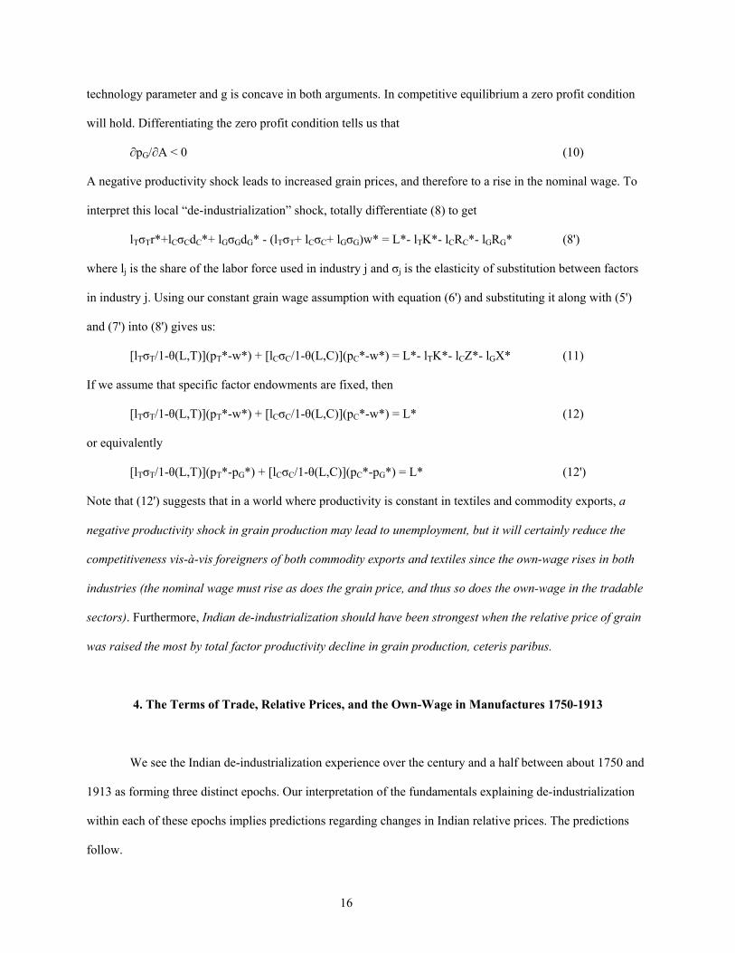
A negative productivity shock leads to increased grain prices, and therefore to a rise in the nominal wage. To

interpret this local “de-industrialization” shock, totally differentiate (8) to get

lTσTr*+lCσCdC*+ lGσGdG* - (lTσT+ lCσC+ lGσG)w* = L*- lTK*- lCRC*- lGRG* (8')

where lj is the share of the labor force used in industry j and σj is the elasticity of substitution between factors

in industry j. Using our constant grain wage assumption with equation (6') and substituting it along with (5')

and (7') into (8') gives us:

[lTσT/1-θ(L,T)](pT*-w*) + [lCσC/1-θ(L,C)](pC*-w*) = L*- lTK*- lCZ*- lGX* (11)

If we assume that specific factor endowments are fixed, then

[lTσT/1-θ(L,T)](pT*-w*) + [lCσC/1-θ(L,C)](pC*-w*) = L* (12)

or equivalently

[lTσT/1-θ(L,T)](pT*-pG*) + [lCσC/1-θ(L,C)](pC*-pG*) = L* (12')

Note that (12') suggests that in a world where productivity is constant in textiles and commodity exports, a

negative productivity shock in grain production may lead to unemployment, but it will certainly reduce the

competitiveness vis-à-vis foreigners of both commodity exports and textiles since the own-wage rises in both

industries (the nominal wage must rise as does the grain price, and thus so does the own-wage in the tradable

sectors). Furthermore, Indian de-industrialization should have been strongest when the relative price of grain

was raised the most by total factor productivity decline in grain production, ceteris paribus.

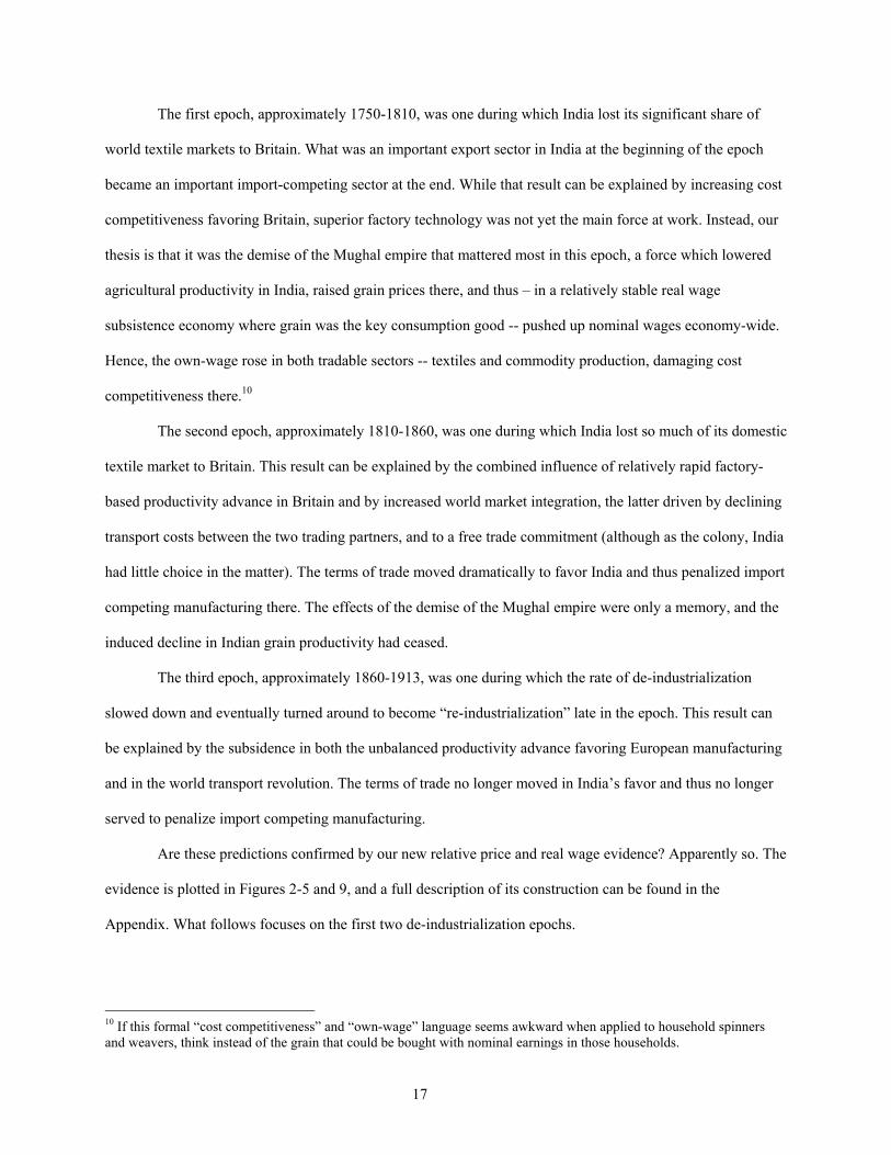
4. The Terms of Trade, Relative Prices, and the Own-Wage in Manufactures 1750-1913

We see the Indian de-industrialization experience over the century and a half between about 1750 and

1913 as forming three distinct epochs. Our interpretation of the fundamentals explaining de-industrialization

within each of these epochs implies predictions regarding changes in Indian relative prices. The predictions

follow.

17

The first epoch, approximately 1750-1810, was one during which India lost its significant share of

world textile markets to Britain. What was an important export sector in India at the beginning of the epoch

became an important import-competing sector at the end. While that result can be explained by increasing cost

competitiveness favoring Britain, superior factory technology was not yet the main force at work. Instead, our

thesis is that it was the demise of the Mughal empire that mattered most in this epoch, a force which lowered

agricultural productivity in India, raised grain prices there, and thus – in a relatively stable real wage

subsistence economy where grain was the key consumption good -- pushed up nominal wages economy-wide.

Hence, the own-wage rose in both tradable sectors -- textiles and commodity production, damaging cost

competitiveness there.10

The second epoch, approximately 1810-1860, was one during which India lost so much of its domestic

textile market to Britain. This result can be explained by the combined influence of relatively rapid factory-

based productivity advance in Britain and by increased world market integration, the latter driven by declining

transport costs between the two trading partners, and to a free trade commitment (although as the colony, India

had little choice in the matter). The terms of trade moved dramatically to favor India and thus penalized import

competing manufacturing there. The effects of the demise of the Mughal empire were only a memory, and the

induced decline in Indian grain productivity had ceased.

The third epoch, approximately 1860-1913, was one during which the rate of de-industrialization

slowed down and eventually turned around to become “re-industrialization” late in the epoch. This result can

be explained by the subsidence in both the unbalanced productivity advance favoring European manufacturing

and in the world transport revolution. The terms of trade no longer moved in India’s favor and thus no longer

served to penalize import competing manufacturing.

Are these predictions confirmed by our new relative price and real wage evidence? Apparently so. The

evidence is plotted in Figures 2-5 and 9, and a full description of its construction can be found in the

Appendix. What follows focuses on the first two de-industrialization epochs.

10 If this formal “cost competitiveness” and “own-wage” language seems awkward when applied to household spinners and weavers, think instead of the grain that could be bought with nominal earnings in those households.

18

Let us begin with the terms of trade. Unfortunately, Figure 9 is only able to document the terms of

trade starting 1800, but it shows two big spurts in the second epoch, the first over the decade of the 1810s and

the second over the decade of the 1850s. If there is any trend in the terms of trade favoring India (and thus

penalizing the import competing sector), it is very modest. But Px/Pm only measures the relative prices

between the two tradable sectors. What about both tradable sectors relative to the non-tradable grain sector?

Figure 2 shows that, relative to grains, the price of both agricultural commodities (Pc) and textiles (Pt) fell

after 1810 and especially after 1815. Only after the 1830s, did commodity production break away from this

trend. Textiles did not do the same.

Now let us consider relative price behavior across the first two epochs combined (also Figure 2).

Between 1765 and 1810, the price of textiles relative to grains fell at a spectacular rate: by 1805-1810, it was

less than 20 percent of its 1765-1770 level. The decline continued after 1810, but at a much slower rate. Why

the spectacular fall in Pt/Pg in the late 18th century, especially compared with the early 19th century? The

answer is that grain prices, while volatile in the short run, soared upwards in the long run. Did this reduce real

wages (w/Pg)? Apparently not: according to Mukerjee (Figure 1), the grain wage did not fall at all between

1729 and 1807; Figure 3 confirms Mukerjee’s claim for roughly the same years, between the 1720s and the

1810s; and according again to Figure 3, the grain wage fell only very modestly between the late 1760s and the

1810s. While there was great short run volatility in the grain wage, a Lewis-like assumption about long run

real wage stability seems to be confirmed for the first epoch. Note, however, that the own-wage in Indian

manufacturing (Figure 4: w/Pt) more than doubled between 1765 and 1810! Since there is no qualitative

evidence suggesting significant productivity advance in Indian textiles and other manufacturing production

during this epoch, we take this evidence as powerful support for the thesis that the demise of the Mughal

empire can indeed explain much of India’s pre-1810 de-industrialization and loss of world markets. India lost

much of its cost competitiveness as the own-wage in home manufacturing underwent that spectacular rise, and

it was the rise in the price of non-tradable grains that pushed up the nominal wage to such high levels.

Grain prices stopped their rise after around 1810, and the upward pressure on nominal wages eased. In

the second epoch, conditions in the grain sector stabilized; now it was the fall in Pt which dominated de-

19

industrialization conditions in Indian manufacturing. The relative price Pt/Pg fell (Figure 2), the own-wage

w/Pt rose (Figure 4), and de-industrialization continued – but now driven solely by world market forces.

If we take the own-wage in manufacturing as a critical indicator of cost competitiveness in India, and

if England was India’s main competitor in world markets, how do trends in the own-wage in textiles compare

between the two? We must be cautious here, since a measured increase in the ratio of Indian to English w/Pt

will be understated to the extent that English productivity growth performance was superior to India even

before the great factory boom. Our source for England is Gregory Clark (2004: Table 6 for nominal wages;

Table 4 for grain and clothing prices), whose data allow us to construct the price of clothing relative the grain

(Pt/Pg) 1705-1865 and the own-wage in textiles (w/Pt). Figure 5a plots an index of the ratio of English Pt/Pg to

Indian Pt/Pg. The Indian series uses decadal averages due to the volatility of Pg in India, and thus starts in

1775, the end of the first decade for which we have data. The price of textiles relative to grains fell in both

economies 1765-1850, but it fell five times faster in India. Pt/Pg fell much slower in England than India (due to

the much bigger Pg boom in India) so that the index rose to 228 by 1815, and again to 421 by 1845. Grain

prices rose almost four times faster in India than England, an event which we argue put greater upward

pressure on wage costs in India than England, thus lowering the English own-wage in textiles relative to India.

Indeed, the ratio of w/Pt in England relative to India fell from 100 in 1775, to 56 in 1815, and to 26 in 1845 as

shown in Figure 5b. More than half of that century fall was completed by 1805, before the great flood of

factory-produced textiles hit Indian markets in the second epoch of de-industrialization.

If we had Indian data for 1705-1765, we think it would extend these trends backwards. After all, in

England Pt/Pg declined only modestly between 1705 and 1765, and w/Pt hardly changed at all. Our guess is

that Pt/Pg fell sharply in India given that Pg about doubled between 1704-1706 and 1764-1766. We think all of

this evidence points to the decline in the Mughal empire as the central cause of Indian de-industrialization in

the 18th century.

20

5. How Do Indian Relative Price Trends Compare with the Rest of the Periphery?

De-industrialization appeared everywhere around the 19th century periphery, and globalization plays a

major role in each region’s economic history narrative. Oddly, however, it is rare for any of these regional

economic histories to make comparative quantitative assessments.11 Here we ask whether 19th century India

faced a big or a small de-industrializing global price shock compared with other parts of the periphery. If it

was “small,” then domestic de-industrialization forces must have been relatively important in India.

If we ignore the few years around 1820 when the terms of trade spikes, it appears that India underwent

a relatively modest improvement in its terms of trade from 1800 to the mid-1820s, and in fact it fell thereafter

up to 1850 (Figure 9). Over the half century between 1800-1804 and 1855-1859, India’s terms of trade rose

“only” 28.6 percent, or less than 0.5 percent per annum. In contrast, the Egyptian terms of trade rose by two

and a half times between 1820-1824 and 1855-1859, or 2.7 percent per annum (Figure 6); the Ottoman terms

of trade increased by two and a half times between 1815-1819 and 1855-1859, or 2.4 percent per annum

(Figure 7); and the Latin American terms of trade increased by 1.7 times between 1820-1824 and 1855-1859,

or 1.7 percent per annum (Figure 8).

In short, it looks like the external price shocks facing India were quite modest compared to the rest of

the periphery. Yet, Indian historians complain the most about de-industrialization. Can we therefore conclude

that domestic supply side conditions played a far more important role in accounting for de-industrialization in

India than elsewhere? And is it only a coincidence that “re-industrialization” in the much of the periphery

starts after the 1860s when the rise in their terms of trade stops (except for export-booming Latin America)?

6. Conclusions

India underwent de-industrialization during the late 18th and early 19th centuries. We can distinguish

two main epochs of de-industrialization that have different underlying root causes. The first epoch runs from

11 For example, there appears to be only one exception in the Ottoman economic history literature, that of Şevket Pamuk (1987). We have found no exceptions in the Indian economic history literature.

21

about 1750 to 1810 and resulted from the collapse of the Mughal empire. As central authority waned, revenue

farming expanded, the rent burden increased, and regional trade within the sub-continent declined, all serving

to drive down the productivity of foodgrain agriculture. Grain prices rose, and given that ordinary workers

lived near subsistence, the nominal wage rose as well. As a consequence, the own-wage in Indian textile

manufactures increased, hurting India’s competitiveness in the export market. India thus lost ground to Britain

in the world textile market during a period when most British production was still carried out using the cottage

system. This version of events is also supported by Bairoch’s evidence that in the second half of the 18th

century India’s share of world industrial production fell faster than in any other part of the non-European

world. During the second epoch, running from roughly 1810 to 1860, productivity advance resulting from the

adoption of the factory system drove down the world price of textiles. The productivity of Indian agriculture

improved during this period under the relative security of Company rule, and grain prices stabilized. The

relative price of grain continued to rise, however, since the world price of textiles continued its secular fall.

By 1860, India had completed a century-long two-part transition from being a net exporter to a net

importer of textiles. Indian de-industrialization was about over.

22

References

Robert C. Allen (2001), AReal Wages in Europe and Asia: A First Look at the Long-Term Patterns,@

unpublished (August).

Amiya Bagchi (1976a), ADe-industrialization in India in the Nineteenth Century: Some Theoretical

Implications,@ Journal of Development Studies 12 (October): 135-64.

Amiya Bagchi (1976b), “Deindustrialization in Gangetic Bihar 1809-1901,” in B. De et al., Essays in Honour

of Prof. S. C. Sarkar (New Delhi: People’s Publishing House).

Paul Bairoch (1982), AInternational Industrialization Levels from 1750 to 1980,@ Journal of European

Economic History 11 (Fall): 269-333.

Lance Brannan, John McDonald and Ralph Schlomowitz (1994), ATrends in the Economic Well-Being of

South Indians under British Rule: The Anthropometric Evidence,@ Explorations in Economic History

31 (April): 225-60.

K. N. Chaudhuri (1978), The Trading World of Asia and the English East India Company, 1660-1760

(Cambridge: Cambridge University Press).

Colin Clark (1950), Conditions of Economic Progress. 2nd Ed. (London: Macmillan).

Phyllis Deane and W. A. Cole (1967), British Economic Growth, 1688-1959: Trends and Structure

(Cambridge: Cambridge University Press, 2nd. ed.).

Jan De Vries (1994), “The Industrial Revolution and the Industrious Revolution,” Journal of Economic

History 54 (June): 249-70.

Javier Cuenca Esteban (2001), “The British balance of payments, 1772-1820: India transfers and war finance,”

Economic History Review LIV (1): 58-86.

Romesh Dutt (1960), The Economic History of India, vol I, Under Early British Rule, 1757-1837 (2 vols; 2nd

ed.; London 1906; repr. Delhi: Government of India Publications Division).

Holden Furber (1948), John Company at work: A Study of European Expansion in India in the Late Nineteenth

Century (Cambridge, Mass.: Harvard University Press).

23

Mohandas K. Gandhi (1938), Hind Swaraj (Ahmedabad: Navajivan Publishing House, first published in

1904).

Alexander Gerschenkron (1962), Economic Backwardness in Historical Perspective (Cambridge, Mass.:

Harvard University Press).

Irfan Habib (1975), “Colonialization of the Indian Economy, 1757-1900,” Social Scientist 32 (3): 23-53.

Irfan Habib (1985) “Studying a Colonial Economy without Perceiving Colonialism,” Modern Asian Studies

119 (3): 355-81.

Peter Harnetty (1991), “’Deindustrialization’ Revisited: The Handloom Weavers of the Central Provinces of

India c.1800-1947,” Modern Asian Studies 25 (3): 455-510.

Joseph Inikori (2002), Africans and the Industrial Revolution in England (Cambridge: Cambridge University

Press).

Ronald W. Jones (1971), "A Three-Factor Model in Theory, Trade, and History," in J. N. Bhagwati et al. (eds),

Trade, Balance of Payments, and Growth (Amsterdam: North-Holland): 3-21.

Paul Krugman and Anthony Venables (1995), "Globalization and the Inequality of Nations,” Quarterly

Journal of Economics 110 (November): 857-80.

David Landes (1998), The Wealth and Poverty of Nations (New York: Norton).

W. Arthur Lewis (1954), “Economic Development with Unlimited Supplies of Labour,” Manchester School of

Economics and Social Studies 22: 139-91.

W. Arthur Lewis (1978), The Evolution of the International Economic Order (Princeton, NJ: Princeton

University Press).

Angus Maddison (2001), The World Economy: A Millennial Perspective (Paris: OECD).

Ramesh C. Majumdar, H. C. Raychaudhuri, and Kalikinkar Datta (1946), An Advanced History of India

(London: Macmillan).

Karl Marx (1977[1867]), Capital, Volume 1, translated by B. Fowkes (New York: Vintage Books).

Brian R. Mitchell and Phyllis Deane (1962), Abstract of British Historical Statistics (Cambridge: Cambridge

University Press).

Saif Shah Mohammed and Jeffrey G. Williamson (2004), “Freight Rates and Productivity Gains in British

24

Tramp Shipping 1869-1950,” Explorations in Economic History 41 (April): 172-203.

Shiseen Moosvi (2000), “The Indian Economic Experience 1600-1900: A Quantitative Study,” in K. N.

Panikkar, T. J. Byres, and U. Patnail (eds.), The Making of History: Essays Presented to Irfan Habib

(New Delhi: Tulika).

Joel Mokyr (1993), The British Industrial Revolution: An Economic Perspective (Boulder, Col.: Westview

Press).

Morris D. Morris (1983), “The growth of large-scale industry to 1947,” in D. Kumar and M. Desai (eds.), The

Cambridge Economic History of India, II (Cambridge: Cambridge University Press).

Radhakamal Mukerjee (1939), The Economic History of India: 1600-1800 (London: Longmans, Green and

Company).

Jawaharlal Nehru (1947), The Discovery of India (London: Meridian Books).

Prasannan Parthasarathi (1998), ARethinking Wages and Competitiveness in the Eighteenth Century: Britain

and South India,@ Past and Present 158 (February): 79-109.

Tapan Raychaudhuri (1983), “The mid-eighteenth-century background,” in D. Kumar and M. Desai (eds.), The

Cambridge Economic History of India, II (Cambridge: Cambridge University Press).

Tirthankar Roy (2000), The Economic History of India 1857-1947 (Delhi: Oxford University Press).

Tirthankar Roy (2002), “Economic History and Modern India: Redefining the Link,” Journal of Economic

Perspectives 16 (Summer): 109-30.

Colin Simmons (1985), “’De-Industrialization’, Industrialization, and the Indian Economy, c. 1850-1947,”

Modern Asian Studies 19 (3): 593-622.

Daniel Thorner (1962), “De-industrialization in India 1881-1931,” in D. Thorner and A. Thorner (eds.), Land

and Labour in India (Bombay: Asia Publishing House).

Jeffrey G. Williamson (2004), “Explaining World Tariffs 1870-1938: Stolper-Samuelson, Strategic Tariffs and

State Revenues,” in R. Findlay, R. Henriksson, H. Lindgren and M. Lundahl (eds.), Eli F. Heckscher,

1879-1952: A Celebratory Symposium (Cambridge, Mass.: MIT Press, forthcoming).

25

Appendix: The Data

Wages. The nominal wage series for India comes from R. Mukerjee (1939) The Economic History of India:

1600-1800 (London: Longmans, Green and Company). They mostly reflect conditions on the Gangetic plain.

Linear interpolation was used to produce annual estimates from the data, which Mukerjee reported for the

years 1637, 1729, 1751, 1807, 1816, and 1850.

Grain Prices. The grain price index incorporates data from several locations for four key foodgrains in India:

bajra, jowar, rice, and wheat. The index takes an unweighted average across all locations and all grain price

quotes available for any given year. The sources are as follows. Prices of bajra, jowar, and wheat 1700-1750

from the Amber region (near present day Jaipur) are from S. Nurul Hasan, K.N. Hasan, and S.P. Gupta (1987)

“The Pattern of Agricultural Production in the Territories of Amber (c. 1650-1750)” in S. Chandra ed. Essays

in Medieval Indian Economic History (Delhi: Munshiram Manoharlal Publishers). Wheat prices at Delhi 1763-

1835, rice prices at Madras 1805-1850, wheat and jowar prices at Pune 1830-1863, and wheat, jowar, and bajra

prices at Agra City 1813-1833 are from A. Siddiqi (1981) “Money and Prices in the Earlier Stages of Empire,”

Indian Economic and Social History Review (vol. 18, nos. 3-4). Prices of bajra, jowar, and wheat quoted at

Pune 1795-1830 are from V.D. Divekar (1989) Prices and Wages in Pune Region in a Period of Transition,

1805-1830 A.D. (Pune: Gokhale Institute Monograph No. 29. Gokhale Institute of Politics and Economics).

Rice and wheat prices at Fatehpur (in present-day Uttar Pradesh) come from C. W. Kinloch (1852) Statistical

Report of the District of Futtehpore, July 1851 (Calcutta: F. Carbury). Wheat and rice prices at Cawnpore

(present-day Kanpur) are from Sir Robert Montgomery (1849) Statistical Report of the District of Cawnpoor

(Calcutta: J.C. Sherriff). The price of rice at Calcutta 1712-1760 are from K.N. Chaudhuri (1978) The Trading

World of Asia and the English East India Company (Cambridge: Cambridge University Press).

Textile Prices. The bulk of the 18th and 19th century Indian manufacturing sector was involved in producing

cotton textiles. Our textile price series 1765-1820 is constructed by taking the unweighted average of the

import prices of muslin and calico piece goods reported at London and collected by Javier Cuenca Esteban

(underlying his “The British balance of payments, 1772-1820: India transfers and war finance,” Economic

History Review LIV February 2001: 58-86, and sent to us by the author). Since these manufactured goods had

26

high value relative to their bulk, transport costs were a small fraction of their selling price in London by the

late 18th century. The 1820-1850 India textile price series is taken to be the price of cotton piece goods

reported in D. B. and W. S. Dodd (1976) Historical Statistics of the United States from 1790-1970 (University,

Ala.: University of Alabama Press).

Export Commodity Prices. The five key export commodities produced in India during most of the 19th

century were indigo, raw silk, raw cotton, opium, and sugar. Our export commodity price index was created by

weighting the prices of these five commodities by their export shares as reported in K.N. Chaudhuri (1983)

“Foreign Trade and Balance of Payments (1757-1947)” in D. Kumar ed. The Cambridge Economic History of

India v.2 (Cambridge: Cambridge University Press), hereafter Chaudhuri. The Chaudhuri export shares only

begin in 1811, and these (fixed) 1811 shares were used to weight prices in earlier years. Since 18th century

price data for each of the five component commodities begins in different years prior to 1795, the export

commodity price index weights the available prices by their 1811 export shares in a total export that includes

only those commodities for which prices are available. Thus, the weights used in each year always add up to 1.

The coverage of the component series is as follows: indigo, 1782-1850; raw cotton, 1790-1850; raw silk, 1782-

1850; opium, 1787-1850; sugar, 1795-1850. The indigo data is composed of British import prices of Indian

indigo collected by Cuenca Estenban for 1782-1820 and for 1821-1850 British import prices of indigo in

general from the microfilmed supplement to A. D. Gayer, W. W. Rostow, and A. J. Schwartz (1975) The

Growth and Fluctuation of the British Economy, 1790-1850 (Hassocks: Harvester Press), hereafter GRS, for

1821-1850. Raw cotton data are also British import prices of Indian cotton from Cuenca Estenban for 1790-

1831 and British import prices of raw cotton in general from GRS for 1832-1850. Raw silk is composed of

British import prices of Bengal silk from Cuenca Esteban for 1782-1820 and British import prices of raw silk

in general from GRS for 1821-1850. Opium price data are taken from the Calcutta auction price of export

opium recorded in Great Britain, Sessional Papers of the House of Commons (1895: vol. XLII) Final Report of

the Royal Commission on Opium, Part II Historical Appendices, Appendix B 62-63 for 1787-1840 and from

the average revenue yielded per chest of export opium found in J. Richards (2002) “Opium Industry in British

India” Indian Economic and Social History Review (vol. 39, nos. 2-3) for 1841-1850. Sugar prices for 1795-

27

1820 are British import prices of Indian brown sugar from Cuenca Esteban and data for 1820-1850 are British

import prices of sugar in general from GRS.

Terms of Trade. The net barter terms of trade for India 1800-1913 are constructed two ways, labeled

Chaudhuri (1800-1850) and BCW (1800-1913) in Figure 9. The export prices for both methods are the same.

From 1800 to1870, prices for cotton piece goods, raw cotton, raw silk, opium, indigo, and sugar are weighted

by the export shares found in Chaudhuri. Individual commodity price series are as described above in the

textile and commodity price sections. The import price component of the Chaudhuri terms of trade series was

calculated using import shares found in Chaudhuri. Imports were bar iron, manufactured copper, raw wool,

wine, cotton sheeting, and raw cotton, and their prices came from GRS, with the exception of cotton sheeting,

which came from Historical Statistics of the United States from 1790-1970. The import price component of the

BCW terms of trade series for 1800-1870 followed the method used in the BCW database, compiled by Jeffrey

Williamson in his collaborations with Luis BJrtola, Chris Blattman, Michael Clemens and Yael Hadass. U.S.

prices for textiles, metals, building materials, and chemicals and drugs are taken from the Historical Statistics

of the United States from 1790-1970 and are weighted using the fixed weights 0.55, 0.15, 0.075, and 0.075.

The BCW terms of trade series is continued to 1913 by use of the India terms of trade series found in the BCW

database and appendix. This 1870-1913 series, along with terms of trade series for Latin America, the Ottoman

Empire, and Egypt, was first reported in Clemens and Williamson “Where did British Foreign Capital Go?”

NBER Working Paper 8028, National Bureau of Economic Research, Cambridge, Massachusetts (December

2000) which has since been published as “Wealth Bias in the First Global Capital Market Boom 1870-1913,”

Economic Journal vol. 114 (April 2004): 311-44. The BCW appendix describes their construction and it is

available from Williamson upon request.

28

Table 1

Population Dependent on Industry In Gangetic Bihar

1809-1813 1901

Assumption A 28.5% 8.5%

Assumption B 18.6% 8.5%

Source: Bagchi (1976b): Tables 1-5. Note: Under Assumption A, each spinner supports only him or herself, and under Assumption B, each spinner also supports one other person. Under both assumptions, non-spinners are assumed to support the survey’s modal family size (5).

29

Table 2

Percentage of Total Population of Gangetic Bihar Dependent on Different Occupations

1809-1813 1901

Spinners 10.3%

Weavers 2.4%

}1.3%

Other Industrial 9.0% 7.2%

TOTAL 21.6%* 8.5%

Source: Bagchi (1976b): Tables 1-5. * Bagchi reports 18.6%, but this appears to be a mistake.

30

Table 3

World Manufacturing Output 1750-1938 (in percent)

Year India China Rest of the Developed

Periphery Core

1750 24.5 32.8 15.7 27.0 1800 19.7 33.3 14.7 32.3 1830 17.6 29.8 13.3 39.5 1880 2.8 12.5 5.6 79.1 1913 1.4 3.6 2.5 92.5 1938 2.4 3.1 1.7 92.8

Source: Simmons 1985, Table 1, p. 600, based on Bairoch 1982, Tables 10 and 13, pp. 296 and 304. Note: India refers to the total sub-continent.

31

Figure 1Real Wages (w/Pg) in India 1600-1938 from

Mukerjee (1939)

0

50

100

150

200

1600 1729 1816 1870 1890 1911 1928 1938

UnskilledSkilled

32

Figure 2Relative Prices of Tradeables (1800=1)

0

1

2

3

4

1765 1775 1785 1795 1805 1815 1825 1835 1845

Pc/PgPt/PgPt/Pc

33

Figure 3Grain Wage in India 1700-1850 (1800=1)

0

0.5

1

1.5

2

1700 1720 1740 1760 1780 1800 1820 1840

Inde

x

34

Figure 4 Indian Own Wages in Textiles and Agricultural

Commodities (1800=1)

0

1

2

3

4

5

1765 1775 1785 1795 1805 1815 1825 1835 1845

w/Ptw/Pc

35

Figure 5aGrain Price of Textiles in England and India (1775=100)

0

100

200

300

400

500

1705 1715 1725 1735 1745 1755 1765 1775 1785 1795 1805 1815 1825 1835 1845Year

Inde

x

Pt/Pg England / Pt/PgIndiaPt/Pg India

Pt/Pg England

36

Figure 5bTextile Own Wages in England and India (1775=100)

0

100

200

300

400

500

600

700

1705 1715 1725 1735 1745 1755 1765 1775 1785 1795 1805 1815 1825 1835 1845Year

Inde

x

w/Pt England / w/Pt India

w/Pt India

w/Pt England

37

Figure 6Egypt's Terms of Trade 1820-1913 (1880=100)

0

50

100

150

200

250

1820 1830 1840 1850 1860 1870 1880 1890 1900 1910

P CO

TTO

N/P

M

38

Figure 7 Ottoman Terms of Trade 1815-1913 (1858=100)

0

50

100

150

1815 1825 1835 1845 1855 1865 1875 1885 1895 1905

P X/P

M

39

Figure 8 Latin American Terms of Trade 1820-1950

60

70

80

90

100

110

120

130

140

1820 1830 1840 1850 1860 1870 1880 1890 1900 1910 1920 1930 1940 1950

TOT

40

Figure 9India's TOT 1800-1913

0.75

1.25

1.75

2.25

2.75

1800 1810 1820 1830 1840 1850 1860 1870 1880 1890 1900 1910

Year

TOT

Chaudhuri

BCW