DTIC FILE COPY 01

NAVAL POSTGRADUATE SCHOOLMonterey, California

W)0

< DTICELECTE DTHESIS JU 1 S- 199

DTIELECTRONIC COUNTERMEASURES (ECM) ANDACOUSTIC COUNTERMEASURES SUPPORTED

PROTECTION FOR MERCHANT SHIPS AGAINSTSSM/ASM MISSILES AND MINES

by

Bo L. Wallander

December 1989

Thesis Advisor: Robert L. PartelowCo-Advisor: Alan B. Coppens

Approved for public release; distribution unlimited

UNCLASSIFIEDSECURITY CLASSIFICATION OF THIS PAGE

Form ApprovedREPORT DOCUMENTATION PAGE OM No 07040188

la REPORT SECURITY CLASSIFICATION lb RESTRICTIVE MARKINGSUnclassified

2a SECURITY CLASSIFICATION AUTHORITY 3 DISTRiBUTIOt,/AVALABIL1Y OF REPORT

2b. DECLASSIFICATION /DOWNGRADING SCHEDULE approved for public relased;distribution is unlimited

4 PERFORMING ORGANIZATION REPORT NUMBER(S) 5 MONITORING ORGANIZATION REPORT NUMBER(S)

6a NAME OF PERFORMING ORGANIZATION 6b OFFICE SYMBOL 7a. NAME OF MONITORING ORGANIZATION

Naval Postgraduate School (If applicable) Naval Postgraduate School

6c. ADDRESS (City, State, and ZIP Code) 7b ADDRESS (City, State, and ZIP Code)

Monterey, CA 93943-5000 Monterey, CA 93943-5000

8a NAME OF FUNDING/SPONSORING 8b OFFICE SYMBOL 9 PROCUREMENT INSTRUMENT IDENTIFICATION NUMBERORGANIZATION (If applicable)

8c. ADDRESS (City, State, and ZIP Code) 10 SOURCE OF FUNDING NUMBERS

PROGRAM PROJECT TASK WORK UNITELEMENT NO NO NO ACCESSION NO

11 TITLE (Include Security Classification) Electronic Countermeasures (ECM) and Acoustic Countermeasures (ACM)

Supported Protection for Merchant Ships Against SSMASM Missiles and Mines

12 PERSONAL AUTHOR(S) Wal.ander, Bo L.

13a TYPE OF REPORT 13b TIME COVERED 14 DATE OF REPORT (Year, Month, Day) 15 PAGE COUNTMaster's Thesis FROM TO December 1989 196

16 SUPPLEMENTARY NOTATIONThe views expressed in this thesis are those of the author and do not reflect theofficial policy or position of the Department of Defense or the U.S. Government

17 COSATI CODES 18 SUBJECT TERMS (Continue on reverse if necessary and identify by block number)

FIELD GROUP SUB-GROUP ECM, merchant ships, high frequency sonar,sonar design, ACM

19 ABS ACT (Continue on reverse if necessary and identify by block number)

The necessity for merchant ship self protection has become more andmore obvious during recent years. This thesis will investigate thethreat (missiles and mines) and associated counter-measures that mightbe installed to provide a reasonable degree of protection. The resultsindicate that it is possible to get protection against a sea-skimmingmissile with a combination of ECM and ESM deployed aboard the ship. Forprotection against the mine threat, a sonar is designed in order togive the ship enough warning time to make an avoiding maneuver. Thesonar investigation indicates the difficulty in designing a sonar thatcan fulfill all design objectives year-round in a complex acousticenvironment. .f

20 DISTRIBUTION; AVA:LAEIITY OF ABSTRACT . 21 ABSTRACT SECURITY CLASSIFICATION

XUNCLASSIFIED/UNLIMITED 0 SAME AS RPT 0 C DTIC USERS unclassified22a NAME OF RESPONSIBLE INDIVIDUAL 22b TELEPHONE (Include Area Code) 22c OFFICE SYMBOL

Robert L. Partelow (408) 484-1551 IDD Form 1473, JUN 86 Previous editions are obsolete. SECURITY CLASSIFICATiON OF T',S PAGE

S/N 0102-LF-014-6603 UNCLASSIFIED

i.

Approved for public release; distribution is unlimited

Electronic Countermeasures (ECM) andAcoustic Countermeasures (ACM) Supported Protectionfor Merchant Ships Against SSM/ASM Missiles and Mines

by

Bo L. WallanderLieutenant Commander, Royal Swedish Navy

Swedish Naval Academy, 1974Swedish Staff and War College, 1987

Submitted in partial fulfillment of therequirements for the degrees of

MASTER OF SCIENCE IN SYSTEM ENGINEERING (EW)

MASTER OF SCIENCE IN ENGINEERING ACOUSTICS

from the

NAVAL POSTGRADUATE SCHOOLDecember 1989

Author: U'-"U- t(t-kBo Wallaner

Approved by:Roe-'t P tel, Thesis Advisor

A an p ns,c- vis r

Sc H H ey, Second eader

-AA. Atch~ey/Chairman,Engineering Ac° s ics sJthAcademiciran Committee

J6 Sternberg, thairman,Electronic Warfare Academic Group

ii.

ABSTRACT

The necessity for merchant ship self protection has

become more and more obvious during recent years. This

thesis will investigate the threat (missiles and mines) and

associated counter-measures that might be installed to

provide a reasonable degree of protection. The results

indicate that it is possible to get protection against a

sea-skimming missile with a combination of ECM and ESM

deployed aboard the ship. For protection against the mine

threat, a sonar is designed in order to give the ship enough

warning time to make an avoiding maneuver. The sonar

investigation indicates the difficulty in designing a sonar

that can fulfill all design objectives year-round in a

corplex acoustic environment.

Accession PorNTIS GRA&IDTIC TABUnannouncedjustificatio

ByDistribution/_

Availbility Codes

Ava-il and/orDist Special

iii.

TABLE OF CONTENTS

I. INTRODUCTION ........... ...................... 1A. BACKGROUND .......... .................... 1B. DISCUSSION .......... .................... 3C. OBJECTIVES AND CONSTRAINTS ..... ............ 4

II. TARGET SCENARIO ..... .................... 5A. TARGET CHARACTERISTICS...............5

B. OPERATIONAL CONSIDERATIONS ...... ............ 5C. PERFORMANCE ..................................... 7D. RADAR CROSS SECTION ........ ................ 8E. SELF NOISE STUDY ....... ................. 11

1. Propulsion machinery ..... ............. .142. Propulsors ....... ................. 163. Flow over hull noise .... ............. 184. Conclusion ....... .................. 21

III. THREAT SCENARIO ........ .................... 22A. MISSILE THREAT ....... .................. 22

1. Definition of the threat .... ........... 222. Design principles ..... ............... .243. Dimensions and performance ... .......... .264. Missile seeker ................. 27

a. Radar search mode..............28

b. Radar tracking mode ..... ............ .28c. Tracking parameters ..... ............ .28d. ECCM capability ...... .............. .30

B. MINE THREAT ............................ .311. Operational considerations ... .......... 312. Dimensions and performance .... .......... .323. Target strength ..... ............... .34

IV. ELECTRONIC COUNTER MEASURES (ECM) ... ........... .36A. JAMMING ECM ........ .................... .. 37

1. Noise jamming ....... ................. .. 37a. Description ...... ................ .. 37b. Analysis .... ............. 39

(1) Case 1: Selfscreening jamming .... 42(2) Case 2: Side lobe jamming ...... A

c. Discussion ...... ................ 442. Radar Absorbing Materials (RAM) ... ........ .46

B. DECEPTION ECM ........ .................. .. 491. Repeater jamming ...... .............. 49

a. Description ...... ................ .. 49b. Analysis ...... ................. .. 51c. Discussion ...... ................ 53

2. Chaff . . .. ........ ............... .54a. Description ...... ................ .. 54b. Analysis ....... ................ 56c. Discussion ...... ................ 56

iv.

C. DECOYS ......... ...................... 571. Towed Craft ....... .................. 582. Buoys ......... ..................... 613. Rocket decoy ..... .............- . 624. Remotely piloted vehicles (RPV) ... ........ 63

D. TACTICS ECM ........ .................... 64E. ECM CONCLUSIONS ....... .................. 64

V. ECM RECOMMENDATIONS ....... .................. 74A. REPEATER JAMMER ....... .................. 74B. GENERAL BUOY DESCRIPTION .... ............. 77C. ESM SUPPORT ................................... 78

1. Signal environment ..... .............. 812. ESM receiver ...... ................. 813. Signal processing ...... ............... 874. User interface ...... ................ 87

VI. ACOUSTIC ENVIRONMENT STUDY ...... ............... 88A. INTRODUCTION ....... ................... 88B. THE BALTIC OCEAN ...... ................. 88

1. Salinity ......... ................... 902. Currents ......... ................... 903. Wind and waves ...... ................ 914. Speed and sound ...... ................ 915. Absorption ....... .................. 92

C. DESCRIPTION OF THE WATER VOLUME .... .......... 92D. AMBIENT NOISE STUDY ..... ............... 92

VII. SONAR DESIGN STUDY ....... ................... 94A. INTRODUCTION ........ ................... 94B. SONAR DESIGN: STEP 1 ..... ............... 99

1. Carrier frequency ...... ............... 992. Transmission Loss (TL) ............. 1033. Resolution, waveform and target detection . . . 107

a. Incoherent detection .... ........... 113b. Coherent detection .... ............ 114

C. SONAR CONCEPT ........ .................. 115I. Case 1: Using ordinary beamforming with a

circular piston .... ............ 1162. Case 2: Using beam focusing .... .......... 117

D. MULTIPATH PROPAGATION STUDY ...... ............ 119E. SONAR DESIGN: STEP 2 ..... ............... 124

1. Back-scattering strength study .. ........ 1242. Beamwidth calculation .... ............ 132

F. TRANSDUCER STUDY ...... ................. 136G. DESIGN SUMMARY ....... . ................ 139

APPENDIX A: GENERAL ARRANGEMENT OF TANKER ... ......... 142APPENDIX B: CRASH STOP AHEAD TEST .... ............. 144APPENDIX C: CRASH STOP ASTERN TEST ..... ............. 145APPENDIX D: MODIFIED ZIP-ZAG TEST .... ............. 146APPENDIX E: TURNING TEST ...... ................. 147

V.

APPENDIX F: REVERSED SPIRAL TEST ..... .............. 148APPENDIX G: ECM ORGANIZATION ...... ............... 149APPENDIX H: CALCULATION OF PULSE DENSITY .... .......... 150APPENDIX I: MAP OVER THE BALTIC SEA .... ............ 152APPENDIX J: WAVE HEIGHT DETERMINATION ... ........... 153APPENDIX K: ABSORPTION IN DB/KB VICE FREQUENCY .. ....... .154APPENDIX L: LOCATION OF REFERENCE WATER VOLUME .. ....... .155APPENDIX M: SPEED OF SOUND PROFILES WITH RAY TRACING . . .. 156APPENDIX N: BOTTOM REFLECTION COEFFICIENT DAGRAMP . ..... 168APPENDIX 0: KNODSEN'S CURVES FOR AMBIENT NOISE . ...... 170APPENDIX P: MISC. CURVES AND DIAGRAMS ... ........... 171APPENDIX Q: BEAM PATTERN CALCULATIONS ... ........... 172APPENDIX R: BEAMWIDTH CALCULATIONS ..... ............. 177

LIST OF REFERENCES ......... ..................... 179BIBLIOGRAPHY .......... ........................ 182INITIAL DISTRIBUTION LIST ....... .................. 183

vi.

LIST OF TABLES

TABLE 1 MANEUVERING DATA FOR REFERENCE TARGET 7

TABLE 2 FLUCTUATION MODELS 11

TABLE 3 VALUES FOR GENERIC MISSILES 27

TABLE 4 PARAMETERS OF SEARCH RADAR 29

TABLE 5 EVALUATION OF JAMMERS 38

TABLE 6 TRACKING SYSTEM GATE SIZES 44

TABLE 7 EVALUATION OF SELFSCREENING

REPEATER JAMMING 67

TABLE 8 EVALUATION OF CHAFF IN LOCK-ON METHOD 68

TABLE 9 EVALUATION OF DECOYS 69

TABLE 10 EVALUATION OF RADAR ABSORBING MATERIAL 69

TABLE 11 EVALUATION OF JAMMER 70

TABLE 12 EVALUATION OF TOWED CRAFT 71

TABLE 13 EVALUATION OF BUOY 71

TABLE 14 EVALUATION OF ROCKET 72

TABLE 15 EVALUATION OF REMOTE PILOTED VEHICLE 72

TABLE 16 RANGE AND POWER REQUIREMENTS

FOR JAMMER BUOY 76

TABLE 17 WAVE HEIGHTS AT ALMAGRUNDETS 91

LIGHTHOUSE (METERS)

TABLE 18 ABSORPTION RATES 102

TABLE 19 TL FOR CARRIER FREQUENCIES, RANGES 106

TABLE 20 APERTURE DIAMETERS 116

TABLE 21 APERTURE RADIUS 118

TABLE 22 RESOLUTIONS 118

TABLE 23 RAYLEIGH PARAMETERS FOR SEA SURFACE 121

TABLE 24 RAYLEIGH PARAMETERS FOR SEA BOTTOM 122

TABLE 25 SCATTERING REGIONS 131

TABLE 26 DETECTION RANGES AND BEAMWIDTHS 133

TABLE 27 SONAR DESIGN RESULT 141

vii.

LIST OF FIGURES

1. Deepsea tanker sizes by delivery date 2

2. Profile of tanker 6

3. Noise sources in ships 12

4. Regions of dominance of the sources

of self-noise 13

5. Self-noise paths on surface ship 14

6. Example of broadband and narrowband components

of a ship signature 15

7. Typical propeller cavitation spectrum 17

8. Example of boundary layer on ships 19

9. Example of missile trajectory 23

10. Missile flight profile 26

11. Beam top view 30

12. Scan top view 30

13. Typical mine shapes and measurements 32

14. Deployed moored proximity mine 33

15. Wave form for swept spot jammer 39

16. Typical jamming situation 40

17. Selfscreening jammer analysis graph 42

18. Example RAM (absorption) 47

19. Example RAM (interfering) 48

20. Example repeater jammer 49

21. The break-lock method 55

22. Corner reflector 58

23. The "Siren" rocket decoy 62

24. Example of a repeater jammer design 77

25. Example of an unfolded ECM buoy 79

26. Simple RWR block diagram 82

27. The crystal video receiver 83

viii.

28. The IFM receiver 84

29. The superheterodyne receiver 85

30. The wideband superheterodyne receiver 86

31. Water balance in the Baltic Sea 89

32. Salinity variations in the Baltic Sea 89

33. The velocity of the deep sea currents

in the Baltic Sea 90

34. The reference sea bottom 93

35. Determining the minimum detection range

and search sector 96

36. Sonar design method 98

37. Reverberation limited performance

of a sonar system 99

38. The LFM waveform advantage 111

39. Difference between an LFM and a CW pulse

on a PPI Ill

40. The near-field characteristics

of an unfocused beam (top)

and a steered focused beam (bottom) 117

41. Propagation paths between transducer and target 120

42. Lambert's law for a scattering surface 123

43. Reverberation and target echo after

transmitting a 500 ms2 pulse 125

44. The back scattering regions 126

45. Bottom backscattering strength as a

function of grazing angle 127

46. Theoretical damping of resonant air bubbles

in water 130

47. Curve for summation of combining levels.

Ltot = Li + L where L1 > L2 132

48. Transducer scan pattern 140

ix.

ABBREVIATIONS

ACM Acoustic Counter MeasuresAGC Automatic Gain Control

AOA Angle Of Arrival

AGPO Angle Gate Pull Of f

ASM Air to Surface Missile

CM Counter Measures

CW Continuous WaveCTFM Continuous Transmitting Frequency Modulation

dwt Deadweight tonnage

d Detection index

DIFM Digital IFM receiver

DT Detection Threshold

EW Electronic Warfare

ECM Electronic Counter Measures

ECCM Electronic Counter Counter Measures

ESM Electronic Support Measures

EOB Electronic Order of Battle

ERP Effective Radiated Power

FM/CW Frequency Modulated Continuous Wave

FFT Fast Fourier Transform

HP Horse Powers

HOJ Home On Jam

I&W Indication and Warning

IFM Instantaneous Frequency Measurement

LO Local oscillator

LFM Linear Frequency modulation

NSL Noise Spectrum Level

NSL(A) Ambient Noise Spectrum Level

X.

NSL(S) Self Noise Spectrum Level

P(D) Probability of Detection

P(FA) Probability of False Alarm

PRF Pulse Repetition Frequency

POI Probability Of Intercept

PPI Plan Polar Indicator

PW Pulse Width

PRI Pulse Repetition Interval

RO/RO Roll On Roll Off

RCS Radar Cross Section

RGPO Range Gate Pull Off

RWR Radar Warning Receiver

RAM Radar Absorbing Material

RPV Remote Piloted Vehicle

SSM Su face to Surface Missile

SSL Source Spectrum Level

SL Source Level

SLL Side Lobe Level

SIGINT Signal Intelligence

TL Transmission Loss

TS Target Strength

VLCC Very Large Crude Carrier

VGPO Velocity Gate Pull Off

WAM Window Addressable Memory

xi.

I. INTRODUCTION

A. BACKGROUND

The increase in threat technology since world war two

has been alarming. A threat of particular concern to world

navies is the anti-ship missile. Computer programmed,

multi-sensor guided, multi-platform delivered missile

systems, aimed at over-the-horizon targets are veryeffective against the warships for which they are designed.

A second threat, of less sophisticated technology but

nevertheless of good effectiveness against warships, is the

mine. Mines can be deployed by all kinds of platforms and

can also be designed for various purposes. However, as

recent events have clearly demonstrated, anti-ship missiles

and mines are also devastating against unarmed merchant

ships. As a result, countries depending on maritime trade

need to enhance their self-protection capabilities.

A merchant ship needs self-protection in two specific

situations. First, when transiting through a defined "war

zone" area and second, when used for logistic support of a

military operation. Both of these situations occurred in the

Falkland war in 1982 and again in the Persian Gulf war in1985 through 1988. If the merchant ships involved in these

operations had been equipped with some kind of

self-protecting systems, many political, economic and

tactical advantages would have been realized.

Over the past 30 years there have been significant

changes in the size, appearance and general characteristics

of ships engaged in international commerce. The design and

construction technology through the period have accelerated

this development and given us new types of ships with the

ultimate goal of increasing ton-miles per day at maximum

1

profit. Containerships, barge carriers, RO/ROs (Roll On Roll

Off) and liquefied gas carriers are some of the newcomers

which are operating worldwide. Few in number, they are

relatively large, fast, and employ the latest technology.

Tankers and other bulk carriers have been in service for

many years and their numbers, size and power have grown

dramatically. Although participating in worldwide

operations, the immense size of some classes limits them to

ternminal ports and routes. Oil, or oil derivatives, are a

vital product for practically all developed countries so

that the transportation of these products has resulted in a

large number of ships of all sizes; from small coastal

tankers to VLCCs (Very Large Crude Carriers) of over 500,000

dwt.

Figure 1 [Ref. 1] shows the sizes of deep sea tankers by

delivery date.

Owr

Dehvery date of new tankers

Figure 1. Deepsea tanker sizes by delivery date

2

The yearly world oil production today (1989) is estimated

to be around 3 billion tons and is increasing. Of this, 1

billion is transported in tankers. With an estimated 60% of

the world reserves located in the Middle East, the demand

for tankers will likely increase.

Today, the tanker fleet consists of 2,500 large ships

(over 10,000 dwt) and represents a capacity of 230 milliondwt. In addition, there are 280 ships capable of carrying

both oil and/or ore and approximately 4,000 small coastal

tankers.

B. DISCUSSION

To maximize profits, shipowner!T are making greatefforts to reduce expenditures. The cost of acquiring

self-protecting systems for a tanker must be weighed againstthe potential cost savings. That is, are the costs resulting

from loss of life or property versus the cost savings from areduction in insurance premiums, enough to offset the costs

of the self-protection systems?

Considerations other than hardware acquisition will also

affect the overall cost of the self-protecting systems. For

example, do the self-protection systems need to have an

operator or operators? Or is training of current crew

members an option? What about maintenance? Portability?

Having to hire additional, specially educated and trainedpersonnel to operate and care for the equipment adds a great

deal of cost to the life cycle of the systems. Therefore,the systems must be easy to operate and maintain. Since the

tanker does not always have to transit "war zones" to get to

its destination, and must keep its time in port to a

minimum, the necessary equipment should be easily installed

and removed.

3

C. OBJECTIVES AND CONSTRAINTS

The focus of this thesis will be to:* Examine the use of Electronic Warfare support in

reducing the anti-ship missile threat.* Give design parameters for a mine hunting sonar system

in order to reduce the mine threat.

The thesis will first study the threat and merchant ship

characteristics. It will then study the EW system(s)

possibilities that can provide a degree of protection, and

give guidelines and suggestions for further investigations.

The thesis will subsequently continue with a mine hunting

sonar design procedure, where design parameters will be

determined based on outlined mission and technical

assumptions and specifications.

In pursuing the objectives, the following constraints

will be considered:* A scenario paralleling the Persian Gulf experiences

of neutral shipping, transiting through defined "warzones," will be used.

* The threat consideration will be a "generic" radarguided missile and a "generic" mine.

* The EW support and Mine huntinq sonar designcharacteristics must be relative y inexpensive,easily installed and removed, nearly autonomous or,if not, very "user friendly."

* The merchant ship is operating alone.

* EW protection will be limited to ESM and ECM support.

* The Acoustic Counter Measure (ACM) will be limited tothe design of a high frequency mine hunting sonar,mounted on the bow of the ship.

* The sonar hardware design and transducer theory(except beam forming) will not be covered.

* The sonar design environment will be limited to aspecific area in the Baltic sea.

4

II. TARGET SCENARIO

A. TARGET CHARACTERISTICS

Besides the fact that ship sizes have been getting

bigger, even the ship proportions have changed

significantly. Length to beam ratios are now typically 5.5

to 6.5, where previously they were in the 7.5 range. The

draft has also increased and has actually made it impossible

for the largest ships to operate normally in almost all

ports of the world. Careful planning is necessary to

determine how best to accomplish the assigned mission within

the unique constraints of each port. In many cases the ship

or ships have to be unloaded outside the port by smaller

tankers. [Ref. 2]

Although a "standard" tanker will be used throughout the

thesis, other tanker dimensions will be considered as

appropriate.

The reference tanker has the dimensions shown in Figure

2. (Ref. 2]

Appendix A shows the general arrangement of typical

"reference" tanker.

B. OPERATIONAL CONSIDERATIONS

During transit through a "war zone" one can assume that

the bridge is manned with at least three persons: one duty

officer, one steersman (no automatic steering during war

zone transit) and one look-out. The alert level is high at

all times. One can also assume that the ship has at least

one X band and a C band radar.

The ship cargo tanks and the bow area are unmanned when

operating at sea. They are also the most insensitive part of

the ship to missile attack. Since crude oil has low

5

Length in meters 330Beam in meters 50Depth in meters 25Draft in meters 20Speed in knots 16HP (horse power) 30,000Propulsion SteamLight ship in tons 30,000Deadweight in tons 250,000Displacement in tons 280,000Length/Depth 12.8Length/Beam 6.3

Figure 2. Profile of tanker

inflammability, it is unlikely that the oil will be ignitedby missile impact. Consequently, if it is impossible toavoid the missile, this is the least vital part of the shipto have hit. The zone extends through approximatelythree-fourths of the ship's length. If the vital one-fourthcan remain relatively undamaged, the VLCC may be able toproceed to the nearest "friendly" port.

Even if a VLCC is capable of withstanding several missilehits without sinking, there are still strong politicalreasons to protect the ship. The recent situation withUnited States' involvement in the Gulf War of 1988 is a good

example.

6

In spite of their size, the VLCCs are occasionallyoperating in narrow straights and close to shore. This leadsto a situation where a missile can be launched from theshore. This thesis will look at both the open sea case,whether the missile is fired from an aircraft or a ship, and

the shore case.

C. PERFORMANCEThis section discusses ship maneuverability limits and

the consequences for missile avoidance. It should be obviousthat a VLCC is not designed for fast maneuvers or speedchanges. However, the vertical semicylindrical bow shaperesulting from a tanker's low speed/length ratio, lowerswater resistance and improves propeller efficiency (Figure2). The resulting ship stability gives the tanker moremaneuverability than its size might indicate.

Table 1 shows maneuvering data for the reference target

[Ref. 3]:

TABLE 1. MANEUVERING DATA FOR REFERENCE TARGET

Crash stop ahead test Appendix B(full load condition)

Crash stop astern test Appendix C(ballast condition)

Modified Zig-Zag test Appendix D(ballast condition)

Turning test Appendix E(ballast condition)

Reversed spiral test Appendix F(ballast condition)

7

Given a nominal speed, for both open-ocean and in-shore

situations, of 16 knots (together with the performance

characteristics above), it takes around 20 minutes for a

fully loaded tanker to stop. If the tanker is in ballast, it

will require only about 14 minutes.

With a maximum rudder deviation (35 degrees port or

starboard) and a 16 knot speed, the angular turning velocity

is 0.7 degrees/second. Therefore, the time required to turn

the ship's head 90 degrees is 2.5 minutes in ballast

condition, and is estimated to be 3.0 minutes when fully

loaded.

These results indicate that to use "speed changes" to

deceive an incoming missile is not effective. However, in

some situations, a tanker at full speed can reduce the

missile's approach angle significantly, within the missile's

flight time, by applying the appropriate full rudder

deviation. This is naturally dependent on what kind of

indication and warning (I&W) the ship has available.

D. RADAR CROSS SECTION (RCS)

The quantitative measure of the ratio of power density

of a radar wave scattered from a target, to the power

density in the radar wave incident upon the target, is

called the radar cross section (RCS) of the target.

It is assumed that the target is in the far field, i.e.,

when the target is sufficiently far from the antenna so that

the incident wave upon the target is approximately planar.

In this case, the radar cross section can be defined as

independent of range to the target. [Ref. 4]

The RCS dimensions are generally expressed as unit square

meters. This convention will be used throughout this thesis.

To get correct values for a target's RCS is very

difficult. There are formulas to calculate theoretical RCS

areas foL a number of standard shapes, but when the targets

8

get more complex, such as with aircraft and ships, there are

no simple relationships to use.

The RCS of complex targets are further complicated by theviewing aspect and the radar frequency. The target comprises

a number of independent shapes and objects which scatterenergy in all directions. The relative phases and magnitudes

of all the scattering shapes contribute differently at the

receiving antenna and give a varying RCS area as the target

shifts in orientation, moves or the viewing aspect is

changed.

The theoretical approach to defining RCS relates incidentto reflected electromagnetic fields and is shown below as

[Ref. 4]:

2E

2 r= lim4ir R.R --- >

where c = RCS

R = Distance between radar and target

Er = Reflected field strength

Ei = Strength of incident field at target

An easier and probably better way of plotting RCS is to

measure the real target in the real (at sea) environment.

Another way is to break up a complex target into a number

of simple geometrical shapes, for which we know the

scattering behavior, and then to compute the sum of their

individual contributions to the whole-target RCS.

A VLCC tanker is considered to be a complex target.

Unfortunately, there is no reliable RCS data available,

using the approaches described above. Therefore, the only

option is to use a simple empirical expression. This

expression assumes a ship target at a shallow grazing angle,

to obtain an average RCS. This means the expected maxima

9

about the port and starboard sides are averaged downward,and the resulting value is a median (50th percentile) RCS.

The RCS formula to be used is shown below and was derivedfrom measurements made at X, S and L bands for ships from2,000 to 17,000 tons. If the formula is valid outside this

size and frequency range, it will give us the numbers shownbelow for the X and the K band radars. [Ref. 4)

c = 52 * F1/ 2 * D3 / 2

where a RCS in m

F = Frequency in MHz

D = Ship's (full load) displacement in kTon

Calculation: for X band radar = 24 million m2

for K band radar = 33 million m2

These numbers are grossly in error when compared withcollected data from other kinds of ships.

The effective radar cross section for the referencetarget is finally estimated to be 100,000 sm average value,valid at all aspect angles and under both loaded andunloaded condition [Ref. 3). This estimation is a compromiseof empirical and measured data. This is a very crude pictureof the reality. For example, there is a significant RCSdifference depending on whether the ship is exposed from thebroad side or from the stern. The fact that the maxima arequite narrow in angle, however, makes this a special casethat can be utilized by an attacking missile only if the

ship is unable to react quickly enough.

As mentioned above, the cross section area of a target inmotion is almost never constant. The variations may be

caused by meteorological conditions, the lobe structure ofthe antenna pattern, equipment instabilities or relative

10

motions of radar and target. The variations due to a complex

target's cross section fluctuations with viewing angle are

considered to be the most sensitive parameters and must be

taken into account.

The easiest and the most economical method for making

adjustments for this is to use the Swerling models (Table

2), where it is possible to adjust the detection

probabilities is terms of four different fluctuating models

of cross section. [Ref. 6]

TABLE 2. FLUCTUATION MODELS

Slow target Fast targetfluctuation fluctuation

Many reflectors

of same size model 1 model 2

One dominantreflector model 3 model 4

In our case, model 3 is the most adequate. A tanker is a

relatively "clean" target, considering its superstructure

(that is, few small reflectors), so the whole ship is

basically one dominant reflector. Further, the missile radar

is typically a tracking radar where the number of radar

returns is large and the RCS area fluctuation is slow.

E. SELF NOISE STUDY

Noise generated by the platform engines and movement

through the water, etc., complicates the sonar detection

process. This self noise is measured in dB re 1i Pa/Hz1 /2

Self noise is entered in the sonar equation as an equivalent

omni-directional noise spectrum level (NSL(A)). The NSL(A)

11

and NSL(S) are competitive, and if one dominates (over 10

dB) the contribution of the other is negligible. [Ref. 7]

The objective will be to determine the major noise

sources of the VLCC tanker and further give an estimation of

the NSL(S) at the sonar location. The assumption for the

discussion is that the tanker is transiting a war zone with

a speed of 16 knots. No measured NSL(S)s for a tanker ofthis size and high sonar frequencies have been found in the

literature.

The most significant noise causes in a ship can be

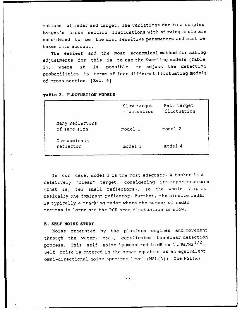
depicted as seen in Figure 3. [Ref. 8]

The general rule is that self noise tends to increase

with the increasing speed of the platform. Further, the

relative importance of the different noise sources can be

seen in Figure 4. The figure shows the areas where the

different noise sources are dominating [Ref. 9).

RADIATED NOISE

MACNINERY IYSROOYNAMICSOURCES SOURCES

PROPULSION MACRINERT AURI IARY MACHINERY FLOW ON'VE ULL

01ESEt EGINES SIEiEL lENERATORS CAVITATION MULL OR SOME CAVITATIONPROPULSION TURNINts TURSOGENERAToRS SINGING VORTEX EXCITED RESONANCESPROPULSION MOTORS PUMPS SLADE OSCILLATING FORCES ESOUNOARY LAYER TURIULENCEGEARS COMPRESSORS RULL OSCILLATING FORCES WAKE TURIULENCIEAtCIPROCATING STEAM MOTORS ROTATION NOTES ('IITINI PRESSURE FIELO OF RULL

E1GNES CONTROL SURFACE OSCILLATING FORCESSTE AM SYSTEM NOISES ELOWERS AND FANS PULSATING EURILESIXKAUST NOISES IITORAI.IL C SYSTEM

PIPELINE SYSTEMS

Figure 3. Noise sources in ship~s

12

Fasi

4Propeller and/or

S~eet ,~hyh1odynomic roise

Amno e t nose

SlowLow

Frequency

Figure 4. Regions ofdominance of the sourcesof self noise

Other important considerations when estimating the self

noise are the location and mounting of the sonar, together

with the search sector. The fact that the purpose of the

sonar is to detect a stationary mine in a limited sector and

in a forward direction reduces the self noise considerably.

The sonar is deployed in the front part of the ship and will

never point in a direction (astern) where most of the noise

sources are located. Further, the high frequency noise

spectrum levels in general are relatively low even at high

speed.

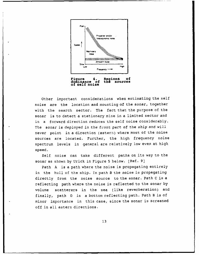
Self noise can take different paths on its way to the

sonar as shown by Urick in Figure 5 below. [Ref. 9]

Path A is a path where the noise is propagating entirely

in the hull of the ship. In path B the noise is propagating

directly from the noise source to the sonar. Path C is a

reflecting path where the noise is reflected to the sonar by

volume scatterers in the sea (like reverberation) and

finally, path D is a bottom reflecting path. Path B is of

minor importance in this case, since the sonar is screened

off in all astern directions.

13

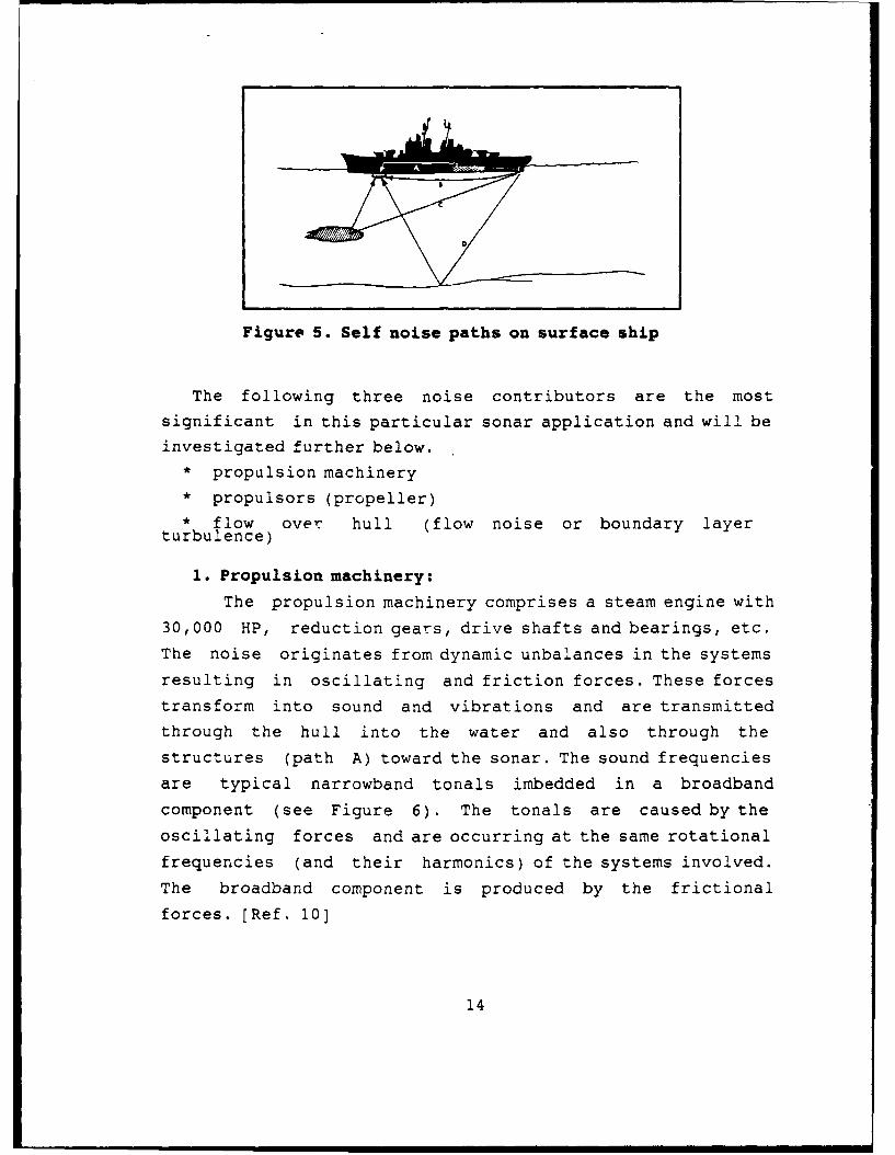
Figure 5. Self noise paths on surface ship

The following three noise contributors are the most

significant in this particular sonar application and will be

investigated further below.* propulsion machinery

* propulsors (propeller)

* flow over hull (flow noise or boundary layerturbulence)

1. Propulsion machinery:

The propulsion machinery comprises a steam engine with

30,000 HP, reduction gears, drive shafts and bearings, etc.

The noise originates from dynamic unbalances in the systems

resulting in oscillating and friction forces. These forces

transform into sound and vibrations and are transmitted

through the hull into the water and also through the

structures (path A) toward the sonar. The sound frequencies

are typical narrowband tonals imbedded in a broadband

component (see Figure 6). The tonals are caused by the

oscillating forces and are occurring at the same rotational

frequencies (and their harmonics) of the systems involved.

The broadband component is produced by the frictional

forces. [Ref. 10]

14

Low speed

Frequency

Figure 6. Example ofbroadband and narrowbandcomponents of a shipsignature

Sound propagating through the structure of the ship

(path A) will be heavily attenuated on its way to the sonar.

According to Kohlman and Plunt [Ref. 11] , the sound will

attenuate on the average of 0.8 dB per frame. For a 300 m

path length, containing 125 frames, this gives an

attenuation of 100 dB. The source strength in an engine room

is assumed to be well below 125 dB re 1 V Pa based on data

regarding noise control in ships [Ref. 8]. Therefore, we can

conclude that the sound factor in path A can be excluded

from the noise contributors. Sound can stili be transmitted

through the hull and into the ocean and eventually reach the

sonar using path C and/or D. This acoustic energy, however,

is typically in the lower frequency range and is more or

less overcome by the much more significant propeller noise.

Vibration is a more complicated problem to analyze.

The major vibrations originate from the machinery, propeller

shaft and propeller, but they also originate when ocean

waves strike the ship as it moves forward. The hull is

vibrating with vertical, longitudinal, horizontal and

torsion vibrations. Other vibrating parts are panels,

superstructures, ,he engine room and the rudder. Vibrations

can be reradiated out by the hull and cause noise. It may

also cause vibrations on the mounting of the sonar which is

a severe problem. [Ref. 9]

15

To theoretically estimate the impact of vibrations in

terms of some kind of noise spectrum level is extremely

difficult and will not be attempted in this thesis. It is

assumed that the design of the sonar hardware, together with

an adequate mounting technique dampens out most vibrations.

Using chock suspensions and making the sonar hardware

resonance frequency higher than the excited vibration

frequencies are some of the actions that can be taken.

2. Propulsors

The major propulsor that produces acoustic noise in

the ocean is the propeller (propeller noise). Propeller

noise consists mainly of cavitation by the rotating

propeller blades and "singing., Cavitation develops when

bubbles behind the propeller blades rapidly collapse. This

produces a broadband acoustic noise signal. The cavitation

noise decreases with depth and increases with propeller

rotation speed. The "singing" phenomena is emanating from

the vibrational excitation of the propeller blades when

water is flowing around them. This builds up tonal

components in the broadband cavitation spectrum. [Ref. 10]

The high design frequencies considered and the long

path length (300m) from the propeller to the sonar location

are factors that, even in this case, help to reduce the

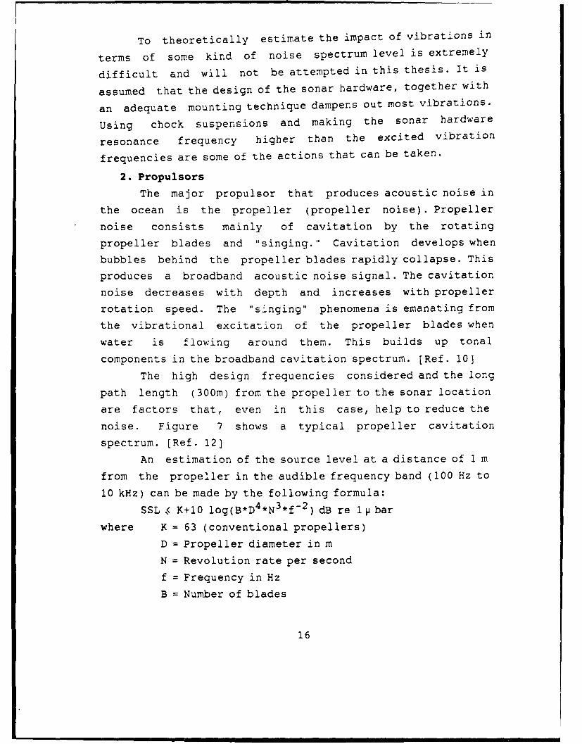
noise. Figure 7 shows a typical propeller cavitation

spectrum. [Ref. 12]

An estimation of the source level at a distance of 1 m

from the propeller in the audible frequency band (100 Hz to

10 kHz) can be made by the following formula:

SSL < K+10 log(B*D4 *N3*f-2 ) dB re l Vbar

where K = 63 (conventional propellers)

D = Propeller diameter in m

N = Revolution rate per second

f = Frequency in Hz

B = Number of blades

16

IIBLD RATE" LINES

E

C

-SLOPE -6dB/OCTAVEIPEAK FREQUENCY'u40- 300 HZ

V-j

-3d8/OCTIVELU

L

C

(n - AUDIBLE FREQUENCIES

10 100 1K 10KFREQUENCY, Hz

Figure 7. Typical propeller cavitation spectrum

This gives for D = 7 m, N = 3 rev/s, f= 10 kHz (upper

limit) and B 4, an estimated SSL of 37 dB re

1 bar/Hz1 /2. The level is then decreasing with -3 dB per

octave which gives

37 -10 dB= 27dB re 1 V bar/Hz1 / 2

or

27 + 100= 127 dB re 1 VPa/Hz1 /2 at 100 kHz

The transmission loss (TL), with an assumption of

spherical spreading, a worst case path length (Path B) of

300 m and an absorption coefficient a=0.02 dB/m gives at the

sonar location [Ref. 12]

17

TL = 20 log R + a*R = 50 + 6 = 56 dB re 1 Pa

The SSL at the sonar location then yields 71 dB re

1 I. Pa/HzI/2 . However, even if this is a significant SSL the

screened-off sonar makes the noise contribution negligible.

The propeller noise will consequently not give a significant

noise contribution. The "singing" overtones might still show

up in the sonar receiver bandwidth, but it is assumed that

this is not very likely to occur. Even if they show up they

can easily be removed by using "notch filters."

Cybulski [Ref. 13] shows measurements of the noise

spectrum levels (NSL) from a VLCC tanker (dead weight of

271,000 tons) at a speed of 16 knots. The measurements were

performed in a low frequency band (2 to 80 Hz), abeam at a

distance of 360 meters. At 10 Hz the NSL was measured to

about 175 dB re 1 VPa/Hz1 /2 . The slope of the measuring

curve goes negative at higher frequencies and the fall rate

is about -11 dB/octave. This means that the NSL at 100 kHz

is estimated to be (13 octaves * 11 dB) 143 dB re 1

Pa/Hz1 2 This leaves 32 dB re I Pa/Hz1 /2 at 100 kHz,

assuming the slope rate holds through the entire frequency

spectrum. Again, since the sonar is only looking in a very

limited angle ahead and never astern, the propeller noise

contribution can still be assumed negligible.

3. Flow over hull noise

The most significant "flow over hull noise" source is

the "boundary layer turbulence" or "flow noise." Flow noise

is generated in the turbulent part of a boundary layer. A

boundary layer is developed between the hull and a

transitional flow of water when the ship is propagating

through the water. It is defined as the region where the

fluid viscosity is present and it extends from a zero flow

velocity at the hull out to 99% of the free stream velocity.

[Ref. 14]

18

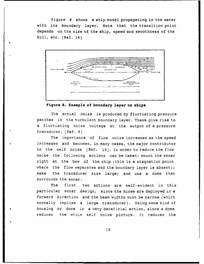
Figure 8 shows a ship model propagating in the waterwith its boundary layer. Note that the transition point

depends on the size of the ship, speed and smoothness of the

hull, etc. [Ref. 14]

6i

;. - - - 11 ON I -1

N'A.

Figure 8. Example of boundary layer on ships

The actual noise is produced by fluctuating pressurepatches in the turbulent boundary layer. These give rise to

a fluctuating noise voltage at the output of a pressure

transducer. (Ref. 93

The importance of flow noise increases as the speedincreases and becomes, in many cases, the major contributor

to the self noise [Ref. 15]. In order to reduce the flow

noise the following actions can be taken: mount the sonar

right at the bow of the ship (this is a stagnation pointwhere the flow separates and the boundary layer is absent);

make the transducer size large; and use a dome that

surrounds the sonar.

The first two actions are self-evident in this

particular sonar design, since the mines are deployed in a

forward direction and the beam widths must be narrow (whichnormally implies a large transducer). Using some kind of

housing or dome is a very beneficial action, since a domereduces the whole self noise picture. It reduces the

19

turbulent flow and hull cavitation and provides space

between the transducer and the flow noise. It is evident

that a sonar dome must be used, mounted on the bow of the

ship as an extension of the bow-bulb. This limits the

flow-noise contributors to the flow-noise surrounding the

sonar dome.

Several measurements have been done in the effort to

estimate the flow noise NSL of different bodies. Urick [Ref.

6] gives NSL values for a transducer located in a buoyant

body and propagating in water at different speeds. According

to these measurements, an extrapolated NSL of 30 - 40 dB re

1 vPa/Hz /2 is given at 100 kHz. Note that there is a

major size and shape difference between the experimental

body and the real sonar dome, though.

Skudrzyk and Haddle [Ref. 15] gives measurements from

an experiment with a rotating cylinder placed in a so-called

"Garfield Thomas Water Tunnel." For a value of S = 0.14

(S = the nondimensional displacement thickness of the

boundary layer at 16 knots. The reference indicates that the

boundary layer thickness S = 5 *8*) and f = 100 kHz, these

measurements give a NSL of about 60 dB re 1 VPa/Hz1 /2 .

There is a significant difference between the results

of the two measurements, which is not surprising since the

assumptions and experimental configurations are different.

However, the experimental set up is more applicable in this

case, even if the measured body is different. Hence, the

values given by Urick [Ref. 9] are probably more accurate to

use in this case.

The NSL in the high frequency part of the spectrum is

also highly influenced by the surface roughness and

smoothness. [Ref. 15] The more grit and/or rust at the

surface, the more noise is generated. Since the sonar system

20

is only deployed for a limited time, a reasonable assumption

is that the sonar dome is always clean and smooth during

operation.

5. Conclusion:

The elimination of many noise sources has been

possible because of the nature of the design problem. The

only noise source that makes a significant impact is the

flow noise. Use of a sonar dome to decrease the flow noise

is necessary. The design of such a sonar dome is beyond thescope of this thesis, but the design requirements are

severe, in order to decrease both the flow noise and the

internal losses.

In order to get a specific number for the NSL the

measurements by Urick [Ref. 9] are probably the most

reliable to use. An upper limit value of 40 V Pa/HzI/2 is

chosen to be the ship's NSL(S) in this particular sonar

application. This upper limit value is assumed to take careof the body size scaling in the experiment and also account

for other small noise contributions.

NSL(S) = 40 dB re 1 i Pa/Hz 1 12

21

III. THREAT SCENARIO

A. MISSILE THREAT

1.Definition of the threat

As mentioned earlier, the missile threat utilized in

this thesis is a surface-to-surface or an air-to-surface

missile (SSM/ASM) whose launch platforms include a ship,

submarine, airplane or missile batteries ashore. Although

both missile types have been available for approximately 40

years, it was not until they had been used in a battle, suchas the war between Israel and Egypt in 1967, that their

effectiveness was firmly established. As a result of thisdemonstration and technical development, very

cost-effective, capable systems have entered the inventories

of almost all countries having military forces.

The most applicable missiles used against a surface

target are the "sea skimmers," most threateningly those with

long stand-off or over-the-horizon capabilities [Ref. 16].

These missiles are designed to fly just above the ocean

surface to make them more difficult to detect, apply ECM orshoot down. To achieve long stand-off distances themissile's trajectory toward the target is usually separated

into three phases.

First comes the boost phase where the missile is

separated from the host carrier, usually to a high altitude.

Then comes the midcourse phase where the missile is guided

with some kind of passive navigation system and also

descends to low altitude at some point in the phase. In this

phase the goal is to avoid any kind of electro-magneticradiation to prevent detection. The third phase is the

terminal guidance phase where the missile utilizes its

22

tracking radar system to get close enough to the target

for proper fuze operation and target damage.

Some of the guidance methods being used are pureinertial navigation, active mapping by radar or juststraight dead reckoning. To keep the altitude s.le during

the terminal phase, some sort of altimetry is used. Since

the missile is flying at relatively low altitudes, a low

power FM/CW radar altimeter using very short wavelengths can

be employed. The FM/CW radar radiates a frequency modulated

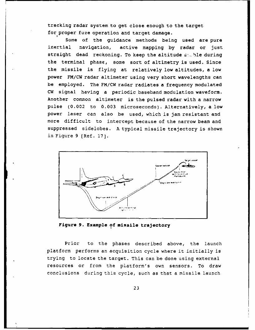
CW signal having a periodic baseband modulation waveform.Another common altimeter is the pulsed radar with a narrowpulse (0.002 to 0.003 microseconds). Alternatively, a lowpower laser can also be used, which is jam resistant andmore difficult to intercept because of the narrow beam andsuppressed sidelobes. A typical missile trajectory is shown

in Figure 9 [Ref. 17].

Tv .t 'OSS64

i , , ! .lock.-On

Figure 9. Example of missile trajectory

Prior to the phases described above, the launchplatform performs an acquisition cycle where it initially istrying to locate the target. This can be done using external

resources or from the platform's own sensors. To drawconclusions during this cycle, such as that a missile launch

23

against one's ship is imminent, needs both sophisticated ESM

equipment and well-trained personnel. Neither are available

onboard our reference ship, hence this acquisition cycle

will not be further investigated.

2. Design principles

There are many ways of estimating an enemy's threat

capability. One method is to determine his electronic order

of battle (EOB). This means that enemy targeting-systems

capabilities are determined through intelligence efforts.

Historically, the intelligence community has been unable to

obtain totally objective information on enemy capabilities,

resulting in a tendency to underestimate (or overestimate)

the threat. Another approach is to assume the enemy has the

same capability that ones own country has, and which you

therefore know quite accurately. Finally, the third

technique is to use a generic design approach, where the

optimum theoretical threat parameters are estimated. Both of

the latter methods have a tendency to overestimate the

threat. Since this is an unclassified thesis, the approach

will be a mix of the two latter methods, but the generic

method will be emphasized [Ref. 18].

Although many missile seeker configurations are

possible, this thesis will only consider a radar guided

missile.

Radars, designed for missile seekers, are often a formof specialized tracking radar whose function is to provide

high data rate guidance information to the missile's control

surfaces. Neither the common tracking nor surveillance radardesigns provide the data rates required. Because the missile

seeker utilizes a narrow beamwidth antenna, more power is

placed on target. The problem with a radar mounted in the

nose of a missile is that the size of the antenna aperture

must be small, on the order of 12 to 40 cm in diameter, and

the capacity to generate high transmitter power is limited.

24

These design considerations must be traded off with the

atmospheric attenuation factors which become more

significant as the frequency increases and the flight

altitude decreases. In general, at low altitudes, the radar

efficiency falls off above X-band at a rate inversely

proportional to frequency.

The missile seeker design has significantly improved

in the last few years. A modern missile seeker is provided

with digital processing, frequency agility, selectable

search patterns and modes, target choice logic (to select

the most important ship in a ship formation) and

considerable ECCM capabilities. [Ref. 17]

The missile seeker ECCM features become vital during

the missile terminal phase, when the radar seeker becomes

active. At this point,the missile's presence becomes known

and susceptible to CM employed by its intended victim.

Therefore, different ECCM methods must be considered to get

a jam resistant missile. Some of the terminal homing schemes

that can be applicable are as follows:* Active radar with TV scan. The TV scan can be used as

a kind of target identification device where a storedtarget picture is correlated with the real time TVscan.

* ARM. An anti-radiation missile whose mission anddesign are focused only on destroying specificemitters, according to their signature.

* HOJ capability. This is a missile seekercounter-measure designed to destroy the source of thejamming. It is similar to an ARM but less fussy as tosignature identification.

* Command guided missiles. Passive homing on reflectedtar qet signals from a radar illuminator or designatorin the area.

In future missile designs one can also expect further

improvement in seeker systems including multi-guidance

modes, multi-sensors and improved target discrimination

capability. [Ref. 191

25

The missile design characteristics to be considered in

this thesis are [Ref. 20]:* missile dimensions

* missile aerodynamic performance

* seeker performance (power, scan, pulse type, ECCM,etc.).

The following sections in this chapter will determine

the parameters of a generic missile that will be used as the

threat reference in the thesis. Some of the parameter

definitions will be broad in order to provide the

opportunity to conduct performance impact analysis.

3. Dimensions and performance

The dimensions of modern sea-skimming ASM/SSM

missiles do not vary much between designs. One possible

explanation is that the same missile type can be fired from

different weapons platforms. Based on unclassified sources,

the parametric values for the generic missile discussed in

this thesis are listed in Table 3:

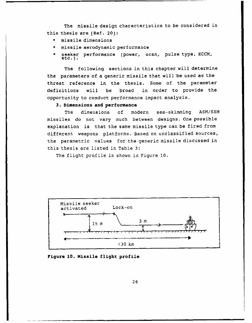
The flight profile is shown in Figure 10.

Missile seekeractivated Lock-on

15m 3m a

<30 km

Figure 10. Missile flight profile

26

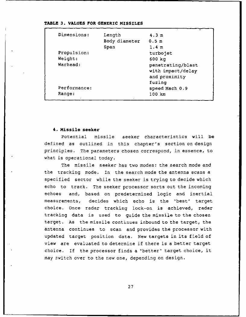
TABLE 3. VALUES FOR GENERIC MISSILES

Dimensions: Length 4.3 mBody diameter 0.5 mSpan 1.4 m

Propulsion: turbojetWeight: 600 kgWarhead: penetrating/blast

with impact/delayand proximityfuzing

Performance: speed Mach 0.9Range: 100 km

4. Missile seeker

Potential missile seeker characteristics will bedefined as outlined in this chapter's section on design

principles. The parameters chosen correspond, in essence, to

what is operational today.

The missile seeker has two modes: the search mode andthe tracking mode. In the search mode the antenna scans aspecified sector while the seeker is trying to decide whichecho to track. The seeker processor sorts out the incoming

echoes and, based on predetermined logic and inertial

measurements, decides which echo is the "best" target

choice. Once radar tracking lock-on is achieved, radartracking data is used to guide the missile to the chosentarget. As the missile continues inbound to the target, the

antenna continues to scan and provides the processor withupdated target position data. New targets in its field ofview are evaluated to determine if there is a better target

choice. If the processor finds a "better" target choice, it

may switch over to the new one, depending on design.

27

a. Radar search mode:

The missile seeker search mode is by active pulsed

radar, utilizing either a fixed frequency or frequency

agility operating in the X-band or K-band, depending on the

design range of the terminal phase. Having a short terminal

phase in future seekers is desirable to reduce the ECM

threat. In addition, frequencies above the X-band will

improve data accuracy. Short terminal phase also means short

reaction time for the target. Future missiles may start

their terminal phase at ranges close to 5 kim, which results

in a reaction time of approximately 15 seconds (assuming a

mach 1 missile). [Ref. 16]

The search radar is not designed to have a big

tanker as its primary target. It is more plausible to assume

that the radar is optimized for a naval combatant such as a

destroyer or a frigate. The radar parameters listed in Table

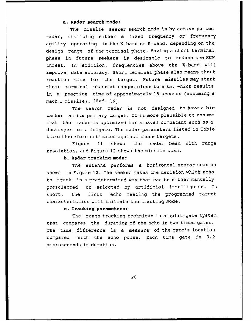
4 are therefore estimated against those targets.

Figure 11 shows the radar beam with range

resolution, and Figure 12 shows the missile scan.

b. Radar tracking mode:

The antenna performs a horizontal sector scan as

shown in Figure 12. The seeker makes the decision which echo

to track in a predetermined way that can be either manually

preselected or selected by artificial intelligence. In

short, the first echo meeting the programmed target

characteristics will initiate the tracking mode.

c. Tracking parameters:

The range tracking technique is a split-gate system

that compares the duration of the echo in two times gates.

The time difference is a measure of the gate's location

compared with the echo pulse. Each time gate is 0.2

microseconds in duration.

28

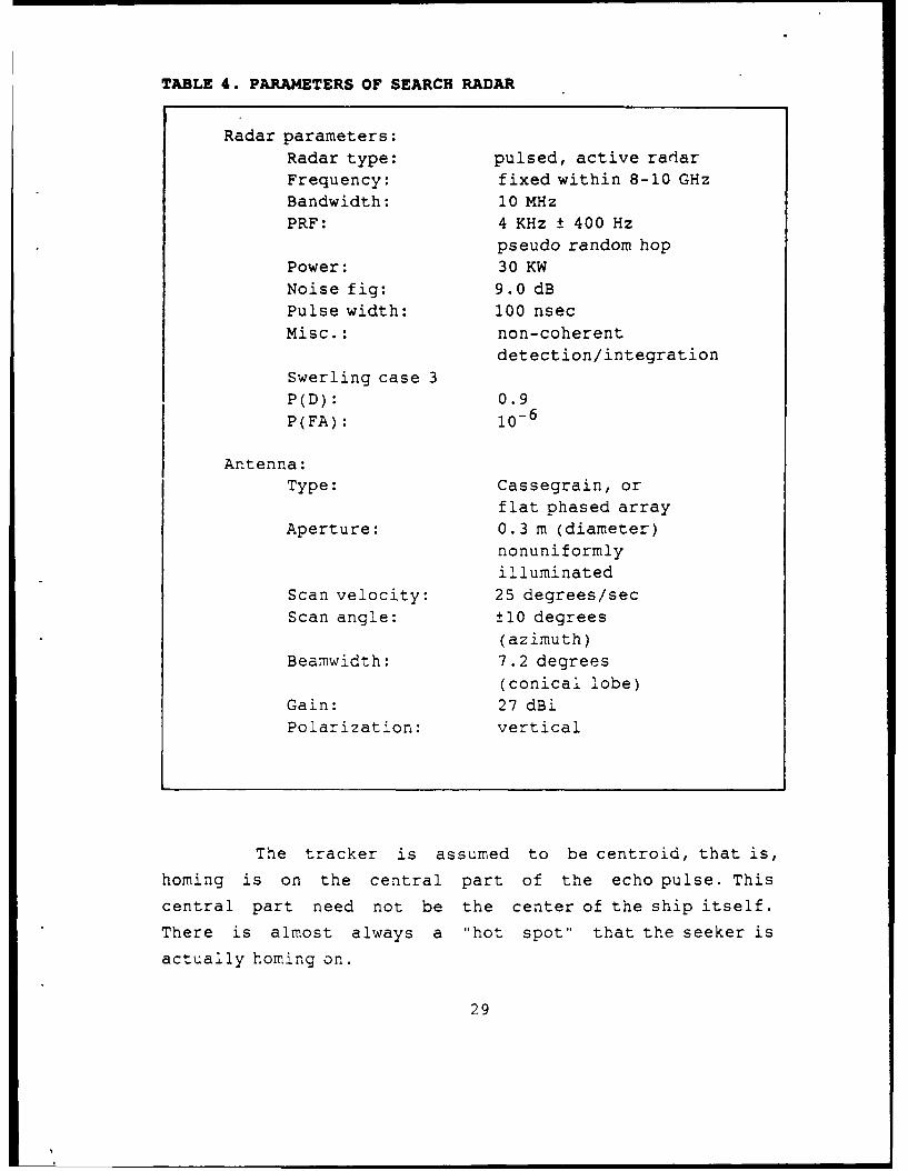
TABLE 4. PARAMETERS OF SEARCH RADAR

Radar parameters:

Radar type: pulsed, active radar

Frequency: fixed within 8-10 GHz

Bandwidth: 10 MHz

PRF: 4 KHz ± 400 Hz

pseudo random hop

Power: 30 KW

Noise fig: 9.0 dB

Pulse width: 100 nsec

Misc.: non-coherent

detection/integration

Swerling case 3

P(D): 0.9

P(FA): 10 - 6

Antenna:

Type: Cassegrain, or

flat phased array

Aperture: 0.3 m (diameter)

nonuniformly

illuminated

Scan velocity: 25 degrees/sec

Scan angle: ±10 degrees

(azimuth)

Beamwidth: 7.2 degrees

(conical lobe)

Gain: 27 dBi

Polarization: vertical

The tracker is assumed to be centroid, that is,

homing is on the central part of the echo pulse. This

central part need not be the center of the ship itself.

There is almost always a "hot spot" that the seeker is

actually homing on.

29

R O

radar R cT/2 rangeresolution

Figure 11. Beam top view

dist max dist

m i~n i t0

Figure 12. Scan top view

d. ECCM capability

In electronic warfare of today, missile seekers

must continue to remain on target in spite of being subject

to a number of ECM techniques (RGPO, chaff, etc.).

Maintaining the seeker effectiveness in the face of the

changing ECM capabilities is a very costly problem for the

designers, but it is a price that must be paid. As much as

50% of the total cost of a missile system can be traced tothe ECCM features in a well-designed system.

This missile is assumed to be equipped with:* HOJ (Home On Jam) capability if other ECCM fails

against active ECM.* Automatic Ein control (AGC) gates to counter

deception ECM.* "Dickie Fix" receiver to counter against swept spot

noise jammer.

30

B. MINE THREAT

The objective of this section is to determine the

target strength (TS) of a "generic" mine. This parameter is

similar to the radar cross section (RCS) for a radar target

discussed in Chapter 2, and will be an important part in the

sonar equations later.

1. Operational considerations

The sea-mine is a very versatile weapon and is used

by almost all countries with a sea border. Some of the

advantages of mines are:* They are relatively inexpensive.

* They can be deployed by almost all kinds of platforms(surface ships, submarines, aircraft etc).

* They can be deployed in covert operations.

* They can be tailored to a particular target andenvironment.

* They are mostly uncontrolled as soon as they aredeployed which implies independence from auxliarysystem(s. c

The major disadvantage with mines is that it is a

relatively slow and stationary weapon system. To sweep mines

and redeploy them in another area is both time consuming and

dangerous.

Mines are often deployed in large numbers and in a

pattern. The area that is sown with mines is termed a mine

field. The outer borders of a mine field are normally very

carefully determined, since the deploying country, in most

cases, wishes to use the water area surrounding the mine

field itself. This is not always true, however. There are

examples of covert mine deployments, such as in the Persian

Gulf, where mines were deployed in ship lanes without any

pattern and in vast water areas.

31

The conclusion is that mines can be used by any nation

in a conflict and they can show up almost anywhere in a "war

zone. "

2. Dimensions and performance

There are a great variety of mines worldwide and

their dimensions and performance depend on their purpose,

environment and the kind of carrier they are to encounter.

This thesis will only consider moored proximity mines since

these are the most appropriate in the outlined scenario. Thewater area considered has a water depth of 100 m which

excludes bottom mines that normally must have a water depth

of less than 50 m to be effective. Also, contact mines just

beneath the surface are very ineffective and seldom used in

modern mine warfare. Moored proximity mines are built by

many countries and some of the typical shapes with

measurements are shown in Figure 13 below. Note that the

mine shell can consist of metal, plastic or cellular

plastics (for reducing TS).

-- I I- I dm

0 2 4 6 8 10

V vV v V V V V

-- T = _

I,/ I 't"=l/I I [ '"l I / / l ( I

f (I ' I { (ff11I

Figure 13. Typical mine shapes and measurements

32

The figure also shows an inside view of the mine.

The mine has a very thin shell and the inside contains a

charge, a sensor with electronics and air. The charge weight

is normally 200 kg and the total weight can be around 900 kg

(with anchor).

Figure 14 shows a deployed moored proximity mine. Notethat the mine depth is approximately 20 m and the proximity

distance is approximately 20 m. The mine depth is optimized

for surface ships.

40 m4120 m

IP

Figure 14. Deployed mooredproximity mine

The performance of mines is a highly classified area,

but in general, mines consist of multiple sensors with

programmable microprocessors to select targets and to resist

countermeasures.

An example of how a mine works is; when a ship comes

in the vicinity of th: mine, say a few nautical miles, an

acoustic sensor alerts the mine. If the sound behavior is

"correct," the mine activates a magnetic and/or a pressure

33

sensor. If the response(s) follows certain conditions the

mine will detonate.

3. Target strength

When a transmitted sound pulse propagates in the

water and impinges on a discontinuity (target) in the water,

some portion of the incident energy will be reflected back

toward the transmitter. This reflected energy is called the

echo and is the signal of interest at the receiver location.

[Ref. 7] "The target strength (TS) is defined as the ratio

of the reflected intensity (Ir) in the receiver direction,

measured 1 m from the effective target center, to the

incident intensity at the same point." [Ref. 10: p. 366]

TS = Ir/I i

The TS depends on the geometry, size and acoustic

impedance of the target. It also depends on the frequency of

the incident signal. In order to get correct TS values the

most adequate way is to measure the particular target under

real conditions. This is not an option in this case,

however. Another possibility is to compare the target with

simple geometrical shapes where TS has been derived. The

problem here is to determine which shape is the mostk

representative to use, among the shapes shown in Figure 13.

Urick [Ref. 9] gives computed TS values for

quasi-cylindrical mines. These values vary between +10 to

-25 dB depending on aspect angle. This indicates at least

the range and magnitudes of the target strength for a mine.

Further issues that need be discussed to get correct

theoretical TS values are: (1) How much of the incident

energy is absorbed by the mine? (2) What is the target

response if sound is penetrating into the mine? (3) Whatkind of resonant effects and vibration modes get excited by

the incident signal and how do these effect the TS?

34

In addition, efforts will be made by the deploying

country to reduce the target strength of the mine as much as

possible. Some of the methods that can be used are listed

below [Ref. 9]:* Anechoic coating

* Viscous absorbers

* Gradual-transition coatings

* Quarter-wave layer

* Active cancellation

These techniques are especially applicable at high

frequencies. The frequency choice in this case is in the

high frequency region, so consequently the TS reduction

techniques must be considered.

The discussion above indicates that to determine a

particular TS value for a "generic" rr,.ne by theoretical

means is not a viable option. instead, let's handle the

problem by assigning a target strength of 0 dB rel.Pa, and

then use the target strength parameters in a sensitivity

analysis at the end of the design study.

TS = 0 dB re 1 v Pa

35

IV. ELECTRONIC COUNTER MEASURES (ECM)

The basic purpose of electronic countermeasures (ECM)

is to introduce wave forms into a hostile electronic system

which will prevent or hamper the system or its operator from

performing their mission.

One way of subdividing the ECM field is shown in Appendix

G. ECM includes jamming, deception and tactics. (Ref. 18]

Jamming is a deliberate radiation or reflection of energy

with the objective of impairing the deployment of electronic

devices used by a hostile force. Deception is the deliberate

radiation or reflection of energy in an effort to mislead a

hostile force. Tactics include what kind of actions the ship

commander can perform to support the jamming and deception

ECM. Only techniques that are applicable to the active sea

skimming missile seeker will be covered.

As mentioned earlier, the seeker has two modes and both

can be affected by ECM. In the search mode the missile

seeker is activated at approximately 20 to 30 km from the

target. Given the 100,000 square meter size of the intended

target, the seeker should be able to immediately "lock on"

the target, assuming no other similar targets are in the

seeker's field of view. It would then switch over to the

tracking mode. The time the seeker spends in the search mode

is therefore assumed to be very short. Because the missile

seeker will spend most of its time in the tracking mode, it

is during this part of the flight profile that the seeker is

most vulnerable to ECM. The thesis will focus on the CM

considerations in this mode.

The main objective for the VLCC tanker is to get the

missile to avoid the target entirely. This includes the case

when the missile misses the target but is sufficiently close

36

to initiate the proximity fuze. If an impact is unavoidable,

a secondary objective is to force the missile to impact the

ship at a point having the least effect on operations.

The purpose of this chapter is to come up with different

ECM support that can be effective for the VLCC tanker

described in Chapter 2.

The advantages and disadvantages of the ECM support willbe documented along with the support's feasibility.

Conclusions will be made at the end of the hapter.

A. JAMMING ECM

1. Noise jamming

a. Description

Noise or "denial" jamming is divided into spotnoise jamming and barrage noise jamming. In principle, spot

noise jamming focuses a narrow band of noise on theoperational bandwidth of the victim seeker. Barrage noise

jamming is broadband and will effect the operation of

seekers emitting within a wide range of frequencies. Spotnoise jamming requires that the seeker operate at one known

frequency unless swept spot noise is employed. If the seeker

utilizes frequency hopping as an ECCM technique, the jammer

must be able to anticipate the seeker frequency changes to

be most effective. This jammer capability is only completely

effective against seekers using a repeated frequency pattern

which can be anticipated by the jammer's frequency

programming logic. Pseudo-random frequency patterns will

degrade a spot jammer's ability to anticipate and jam.

Having a spot jammer capable of following predictable

frequency hoppers will be expensive, swept spot jamming can

be a good compromise. Barrage jamming can cover the

operating frequency range of the seeker, but there is the

penalty of a reduction in Effective Radiated Power (ERP).

Increasing power has the companion constraints of larger

37

size and higher costs. General advantages and disadvantages

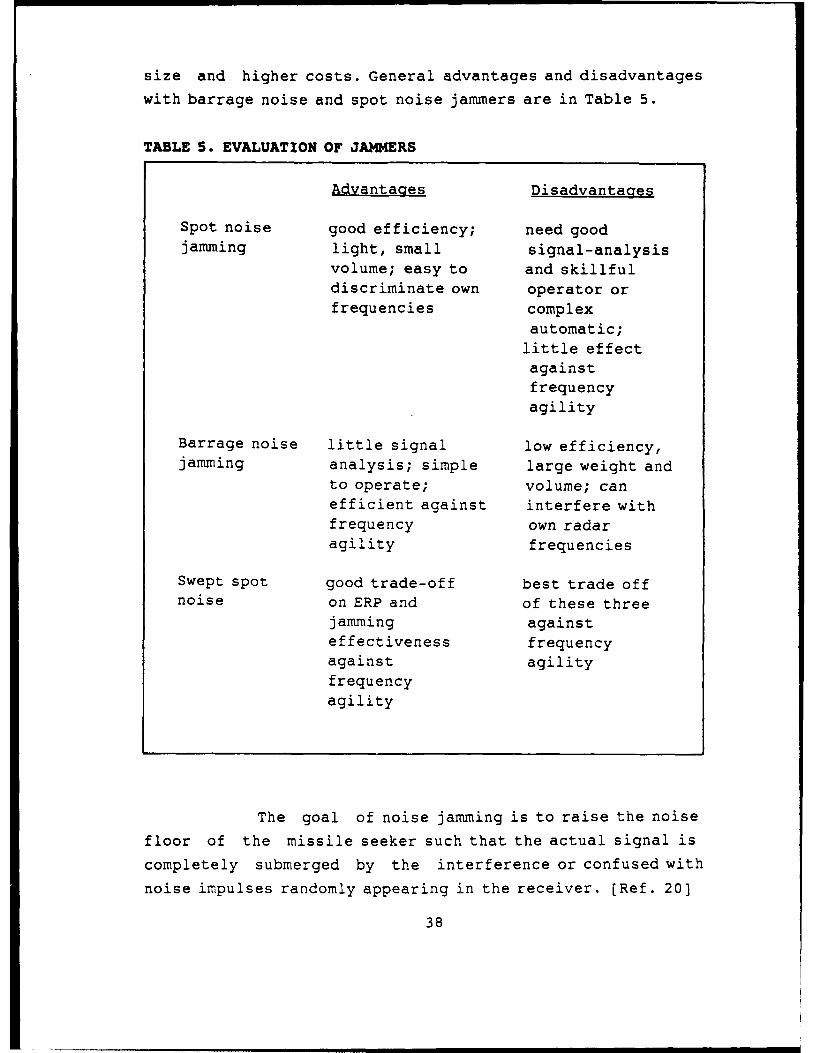
with barrage noise and spot noise jammers are in Table 5.

TABLE 5. EVALUATION OF JAMMERS

Advantages Disadvantages

Spot noise good efficiency; need goodjamming light, small signal-analysis

volume; easy to and skillfuldiscriminate own operator orfrequencies complex

automatic;

little effectagainstfrequencyagility

Barrage noise little signal low efficiency,jamming analysis; simple large weight and

to operate; volume; canefficient against interfere withfrequency own radaragility frequencies

Swept spot good trade-off best trade offnoise on ERP and of these three

jamming againsteffectiveness frequencyagainst agility

frequencyagility

The goal of noise jamming is to raise the noise

floor of the missile seeker such that the actual signal is

completely submerged by the interference or confused with

noise impulses randomly appearing in the receiver. [Ref. 20]

38

The special case of noise jamming called sweptspot jamming, is effectively a combination of barrage noisejamming and spot noise jamming. It utilizes narrow bandnoise that is rapidly swept over a larger frequency band(Figure 15) tRef. 6). Af can be nearly 1 GHz and Tapproximately 1 microsecond.

Swept "sPOt"

i f I -1

Figure 15. Wave form for swept spot jamming

The advantage with this method is that manyseeker frequencies can be jammed at the same time. Thedisadvantage is that the jamming pulse is receivedintermittently, and at a lower rate than the seeker'sreceived echo pulse and is therefore less then 100%effective. This kind of jamming can be substantiallydegraded by incorporating "Dicke Fix" in the seekerreceiver.

b. AnalysisThe target has several ways of utilizing noise

jamming. Some examples are shown below, together withapproximate calculations. All of the values are based on thereference target seeker in Chapter 3.

The following assumptions are made:* free space propagation (no multipath)* no atmospheric attenuation

* no lobe divergence

39

Further, a new reacquisition cycle, that is, when

the seeker is changing target, takes approximately one

second. If the seeker loses information only in onecoordinate (i.e., in range), or is acquiring a new target,

the reaction time is on the order of milliseconds.

One part of evaluating the effectiveness of noisejamming is to mathematically predict burnthrough distance,power requirements, etc. Figure 16 is used throughout this

section of the chapter rRef. 6].

radar f target

Gjt jammer

Figure 16. Typical jamming situation

Abbreviations that will be used for jamming

calculations are.

Pt : radar transmitted powerGt : radar maximum antenna gain

Gtj: radar antenna gain in jammer direction

dt : Gt/Gtj antenna side lobe ratio

Bt : radar bandwidth

Pj : jammer powerGj : jammer maximum antenna gain

Gjt: jammer antenna gain in radar direction

dj : Gj/Gjt jammer side lobe ratio

Bj : jammer bandwidth

40

ds : Bt/Bi bandwidth ratio

7 : target radar cross section area

Rt : distance radar to target

Rj : distance radar to jammer

). : wavelength

Return power at the pulse reflected from the target

into the radar receiver (when the main lobe is pointing on

the target) is:

2P.G G.X

t t a tS

2 2 4w4 rR 4 7.R

t t

Jammer power in the receiver (within the receiver

bandwidth) is:

2P.G G .Aj jt ti

J =d2 4w s

4wR

The general formula for signal to jamming ratio

becomes:

2 2 2P. G .a. R P.G .<7. R.- d. dt t j - tt j jt

S/J = =

4 44 R P G G d 4w. R P G d

t j it tjs t j i S

Assume that the required signal to jamming ratio (for

given values of P(D) and P(FA)) is S/7 min. Assume further

41

that this is achieved at the "burnthrough" distance Rb,

that is (S/J)=(S/J) min for Rt = Rb.(1) Case 1: Selfscreening jamming. This is the

case when the jammer is located on the target or very close

to it. The case is explained in the analysis graph, Figure

17. The location of the jammer is a very important issue

since the missile, if equipped with HOJ capability, probably

will be guided to that location.

power

burn through S/J = 10 dB

II 0S =dB

noise jammer (-20 dB,'decade)

radar ja-_ -er Iradar (-0 dB/dcade)wins wins I noise floor

rangerange rangeb,;rnthrough crossover

Figure 17. Selfscreening jammer analysis graph

Assume a jammer with an antenna gain of 10 dB

and that an (S/J) min ratio of 10 dB is required.

Then the jammer power required for a burnthrough

distance of 600 m (worst case, based on missile

reacquisition cycle and maneuvering capability), and for the

barrage noise jamming becomes:

42

P-G t t

P2 = 66 KWj2

4 ' (S/J)mineG dRjt s b

(Since this is selfscreening jamming, Rj = Rt

and the Gtj = Gt, that is dt = 1.) It also assumes:

10 MHzd s = = 0.05

200 MHz

The jamming power required for spot noise jammingwith the same values as above becomes:

Pj = 3.3 KW, where ds = 1

(2) Case 2: Side lobe jamming. In this case thejammer is external but with approximately the same range to

the missile as the target (Rj = Rt).With t e same assumptions as above, but with

Gtj=Gt , dt=1 and the seeker side lobe ratio of 15 dB

gives:

For the barrage noise case, with dj=l and

dt=15 dB

P G -a.d -dt t j t

P 2 =2.1MWj 2

4 w - (S/J)min GdRjs b

For the soot noise case, Pi = 106 KW

43

The small aperture and the low average transmitted

power in the missile seeker generally results in strong

sidelobes. This makes the missile seeker more vulnerable to

sidelobe jamming. [Ref. 18]

The requirements in both cases described above are

fully achievable with today's techniques.

As shown in Chapter 3, the range tracking system

generates two gates. They are 0.2 V s in duration (that is 60

m) each. The angle tracking resolution (width) depends on

the range to the target and the relationship @ * R, where @(the lobe angle) is expressed in radians. This relationship

gives the following gate sizes shown in Table 6:

TABLE 6. TRACKING SYSTEM GATE SIZES

Range (km) Length (mY Width (m) (cross range)

30 60 3,78020 60 2,52010 60 1,2605 60 630

When these numbers are compared with the target, it

is clear ti.at the reference VLCC tanker, which measures 330

m in length and 50 m in width, can easily fill the gate's

length.

c. Discussion

As stated in Chapter 1, the ECM system must meet

the basic parameters of simplicity, reliability,

effectiveness and low cost. Noise jamming is a very

effective and inexpensive way of denying the missile seeker

target data. Based on information theory, white Gaussian

noise injected into the receiver system provides for the

44

most effective jamming. It is statistically impossible forthe seeker to distinguish between this jamming noise and the

noise generated by the receiver itself. So, if the seeker isexpsed to enough high quality, high power noise jamming,

seeker "break lock" is possible. [Ref. 18]

The major problem with any kind of noise jamming isthat the missile seeker, in almost all cases, is equippedwith HOJ capability (that is, it homes on the jammingsignal). This ECCM technique can be utilized by the targetto guide the missile to a dummy target or to an insensitivepart of the target itself. One solution is to tow a jammer

mounted on a small craft behind the ship. There might be aproblem keeping the craft in position due to the wind,

currents and weight of the tow line, etc. A more fundamentalproblem is how far behind the target must the craft be towed

to effectively lure the missile from the ship? The techniquecan be used both in main lobe and side lobe jamming

depending on the length of the tow line. Another seriousproblem arises when the missile is approaching within 45

degrees of the bow or stern. According to the maneuvering

data discussed earlier, there is not enough time to turn the

ship sufficiently to present the craft mounted jammer to themissile. This situation is natural counter countermeasure

that the launching platform can use against the target.

In the selfscreening jamming case, the jammer islocated on the target, that is, on the ship itself. Oneapproach is to mount the jammer in a location that is

prepared for the impact. For example, one tank section inthe front part of the ship can be kept empty with the jammer

mounted on the deck above it. The intent is to attract themissile so it will do the least amount of damage. However,

the bow/stern missile approach still remains. But, since theaft section is considered to be the most important part ofthe ship, missile impact here must be avoided.

45

Ship maneuvering might have an effect in theselfscreening case. It is probably sufficient to turn theship 45 degrees either way to get enough bearing resolution

for the missile to distinguish the jamming section of theship. To turn the ship 45 degrees takes approximately oneminute. In this time the missile has flown 18 km. So, givenenough warning, say when the missile is still between 20 to25 km from the ship, a ship maneuver could solve this

problem.

Given the advantages and disadvantages of noisejamming discussed above, for a ship with lots of space andno power restrictions, the choice of which system design tochoose is more a matter of cost. Whether a simple radarwarning receiver (RWR) together with a barrage noise jammeror a more complex and sophisticated ESM receiver togetherwith a spot noise jammer is chosen depends on one's

assessment of "cost benefit."

Noise jamming together with a ship maneuver can bean effective way of solving the main objective.

If the missile seeker is not equipped with HOJcapability, the missile will get no target information andwill, with very high probability miss the target. Further,

if HOJ capability exists, the missile is deliberately guided

by the jammer to a expendable dummy target or to a"prepared" section of the ship.

2. Radar Absorbing Materials (RAM)

Different methods have been investigated in the effortto decrease the RCS area for ships, airplanes, missiles,

etc.

The most important and least expensive method is toinitially construct the ship for a low RCS area. Large metalsurfaces with interior orthogonal corners (corner reflectors

effect) must be avoided. Large RCS areas can also beobtained from openings such as ducts that create resonance

46

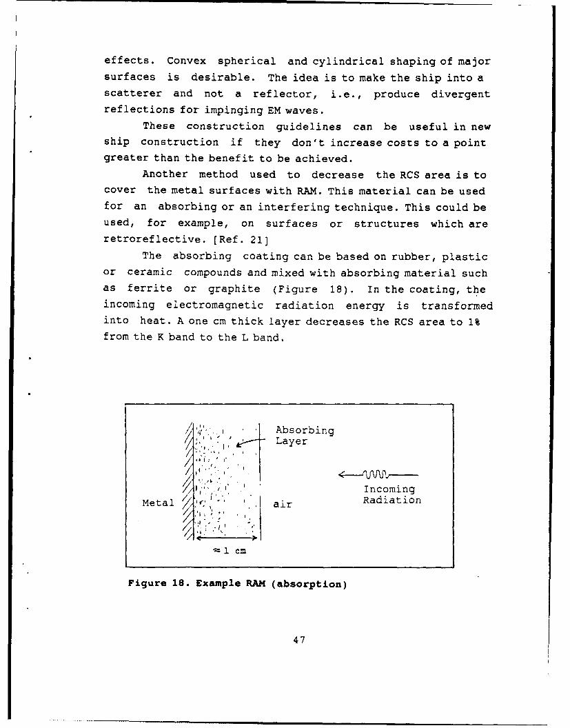
effects. Convex spherical and cylindrical shaping of majorsurfaces is desirable. The idea is to make the ship into ascatterer and not a reflector, i.e., produce divergent

reflections for impinging EM waves.

These construction guidelines can be useful in newship construction if they don't increase costs to a pointgreater than the benefit to be achieved.

Another method used to decrease the RCS area is tocover the metal surfaces with RAM. This material can be usedfor an absorbing or an interfering technique. This could beused, for example, on surfaces or structures which areretroreflective. [Ref. 21]

The absorbing coating can be based on rubber, plasticor ceramic compounds and mixed with absorbing material suchas ferrite or graphite (Figure 18). In the coating, theincoming electromagnetic radiation energy is transformedinto heat. A one cm thick layer decreases the RCS area to 1%from the K band to the L band.

Absorbing7,',, , *,, LLayer

, ,Incoming

Metal air Radiation

1l cm

Figure 18. Example RAM (absorption)

47

The method is expensive and the ship will gain aconsiderable weight if all surfaces are coated. There is aproblem with the strength and durability of these coatings.

[Ref. 6]

The reflecting damping material can also be of aninterfering type. The metal surfaces are painted with asemi-transparent 1/4 wavelength layer, reflecting half andtransmitting half of the energy. The reflected energy is 1/2wavelength out of phase with the transmitted energy causing

destructive interference shown in Figure 19 [Ref. 6]. Thelayer can be designed for any frequency from 400 MHz to 40GHz and the absorption is around 99%. However, the bandwidthis narrow and the effect depends on the angle of incidence.The material is also affected by the sea environment so thatits lifetime is limited. Like the previous method, this isan expensive technique if a whole ship is to be coated. Inaddition, the surface of the ship has to be speciallyprepared to accept the coating.

SemiTransparent IncomingLayer Radiation

/cancellationA C

Metal / Air

Figure 19. Example RAM (interfering)

48

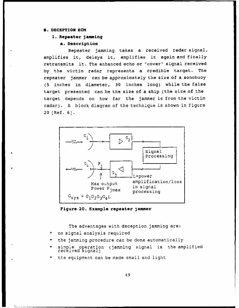
B. DECEPTION ECM

1. Repeater jamming

a. Description

Repeater jamming takes a received radar signal,

amplifies it, delays it, amplifies it again and finally

retransmits it. The enhanced echo or "cover" signal received

by the victim radar represents a credible target. The

repeater jammer can be approximately the size of a sonobuoy

(5 inches in diameter, 30 inches long) while the false

target presented can be the size of a ship (the size of the

target depends on how far the jammer is from the victim

radar). A block diagram of the technique is shown in Figure

20 [Ref. 6].

Signal

Processing

4 P.

G3 iL=power

Max output amplification/lossPower Pjx in signal

jmax processingSy s = GG 2 G3 G4 L

Figure 20. Example repeater jammer

The advantages with deception jamming are:* no signal analysis required

* the jamming procedure can be done automatically

* simple operation (jamming signal is the amplifiedreceived signal)

* the equipment can be made small and light

49

The disadvantages are:

* easy to saturate by other transmitters

* hard to get sufficient isolation between thetransmitting antenna and the receiving antenna.

* unable to reproduce complex wave forms (chirp,mponopulse, e.g.), except when the repeater isincapable of range deception.

The repeater jammer is more complex [Ref. 18] than

the noise jammer and needs a greater amount of processing

power for its implementation.

The three repeater jamming techniques are:* velocity gate pull off (VGPO)

* angle gate pull off (AGPO)

* range gate pull off (RGPO)

The range gate pull off (RGPO) is the most useful

technique in this case. VGPO is mainly useful against radars

using doppler or CW techniques. AGPO techniques can only be

applied when angle gates are being used in the missile

seeker.

The RGPO technique is effective against pulse radar

and the goal is to create a false echo that arrives at the

seeker a little later than the real target echo. The

distance between the missile and the target is then changed

to a false value.

The RGPO technique initially repeats the received

echo with a minimum delay time. The amplitude of the

repeated echo is increased slowly but still with minimum

time delay. This causes the radar automatic gain control

(AGC) to adjust to the stronger echo by reducing the gain.

The real echo amplitude is reduced, causing the seeker to

capture the strong repeated echo instead.

Now, the jammer begins to increase the amount of

time delay in the repeated signal and the range gate

circuitry gradually "walks off" the real target echo. When

50

the jamming signal stops, the tracker has no "skin" data inits range gate and must do a reacquisition cycle.

Since deception is only in range and not in angle,target reacquisition may be very rapid, in a matter ofmilliseconds since the angle information may still be

available.

The best result is achieved with a combination ofthe repeater techniques above causing the reacquisition

cycle to be accomplished in seconds, but combining thetechniques is very hard to achieve.

A special case of repeater jamming (blip enhanceror repeater) is when the signal is intercepted and amplified

as above but is not delayed. This will create a return echosimilar to the target echo and hence, can be used as a

decoy.

b. Analysis

An estimate of the feasibility of using repeaterjamming includes calculations of the system gain and powerrequirements. The assumptions and notations made in Table 4and Figure 16 are used.

The jammer in this chapter is assumed to be on thetarget, i.e., the ship. The jammer retransmitted power is

(Figure 16, p. 40):

2P G GA

t t 1P = - -GLG

j 2 4 ir 2 34 ir R

t

It will be assumed that Pj<Pj max, where Pj

max is the maximum power achievable before the amplifier

gets saturated. The missile seeker then receives the

following power from the jammer:

51

2P.G G.Aj 4 t

J =

2 4ir4,ir- R

t

The seeker receives the following power from the

RCS area of the target:

2PG G.At t or t

S =2 2 41

4 Ir.R 4ir-Rt t

The J/S ratio after the antenna of the missile

seeker becomes:

24 P G .R

j 4 t(J/S) =

P . Gt t

The condition for the jamming to succeed is:

J/S > (J/S) min

where (J/S) min is the smallest jamming signal ratio

necessary to deceive the missile tracker. (J/S) min dependson what kind of jamming is utilized and what kind of

receiver it shall be used against. The (J/S) min is a very

difficult parameter to estimate.

The following two equalities must be fulfilled forsuccessful iamming (where Gs = system gain):

52

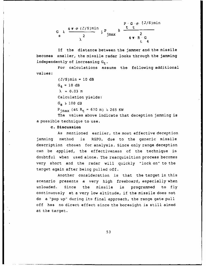
P G a. (J/S)min

G A,4j.q (J/S)min ;Pj a 1 t t 2

s 2 a 24iRGt 4

If the distance between the jammer and the missile

becomes smaller, the missile radar looks through the jamming

independently of increasing Gt.

For calculations assume the following additional

values:

(J/S)min = 10 dB

G4 = 10 dB

= 0.03 m

Calculation yields:

Gs >, 100 dB

Pjmax (at Rt = 670 m) >, 265 KWThe values above indicate that deception jamming is

a possible technique to use.

c. Discussion

As mentioned earlier, the most effective deception

jamming method is RGPO, due to the generic missile

description chosen for analysis. Since only range deception

can be applied, the effectiveness of the technique is

doubtful when used alone. The reacquisition process becomes

very short and the radar will quickly "lock on" to the

target again after being pulled off.

Another consideration is that the target in thisscenario presents a very high freeboard, especially when

unloaded. Since the missile is programmed to fly

continuously at a very low altitude, if the missile does not

do a "pop up" during its final approach, the range gate pull

off has no direct effect since the boresight is still aimed

at the target.

53

2. Chaff

a. Description

Chaff is a passive radar countermeasure. The

"jamming" effect that chaff makes in the radar receiver is

caused by the reflected energy of the active radar

transmitter itself. Chaff is still the most widely used

countermeasure and was first introduced in World War Two.

The material used for chaff today consists of

aluminized glass fibers with a diameter of approximately 0.1

mm. They are easy to disperse, the fall rate is low (0.6

m/s) and the blooming time is fast (in the order of 3-6

sec). [Ref.16]

There are three methods in using chaff to protect

ships against sea skimming missiles. They are:* the deception method

* the lock-on or dilution method

* the break-lock method

The deception method involves trying to confuse the

search and target acquisition radar by increasing the number

of credible targets in the vicinity of the target. This

method can lead to an initial tactical advantage, but the

"real" target will sooner or later be discriminated from the

chaff clouds. This is not a recommended method to use since

the personnel aboard are limited in their ability to handle

the interception and classification of search and

acquisition radars. Also, the great target size together

with long transiting time and large number of acquisition

radars in the environment makes the method very costly and

impractical to use.

The lock-on or dilution method uses a number of

chaff clouds deployed in a specific pattern around the

target in order to distract the missile seeker ideally

causing it to lock-on the chaff cloud (false target) instead

of the real target. This method is appropriate in the

54

missile seeker's search mode. The search mode in this case

though, is assumed to be very short. Together with the great

target size and the same practical problems encountered with

the deception method above, the lock-on method is a poor

choice as well.

In the break-lock method, the missile has already

locked on to the target and the goal is to seduce the seeker

to lock on to a large chaff cloud deployed within the

seeker's field of view. Once the seeker has locked on to the

chaff cloud, the ship can maneuver out from the cloud (if

the warning time is enough) or use the cloud as an extension

of the ship in order to ensure a "close" miss by the

missile.[Ref. 16]

Because the break-lock method is the only viable

choice, it will be further investigated. It is shown in

Figure 21. [Ref. 16]

12. 3.

" 01

Figure 21. The break-lock method

55

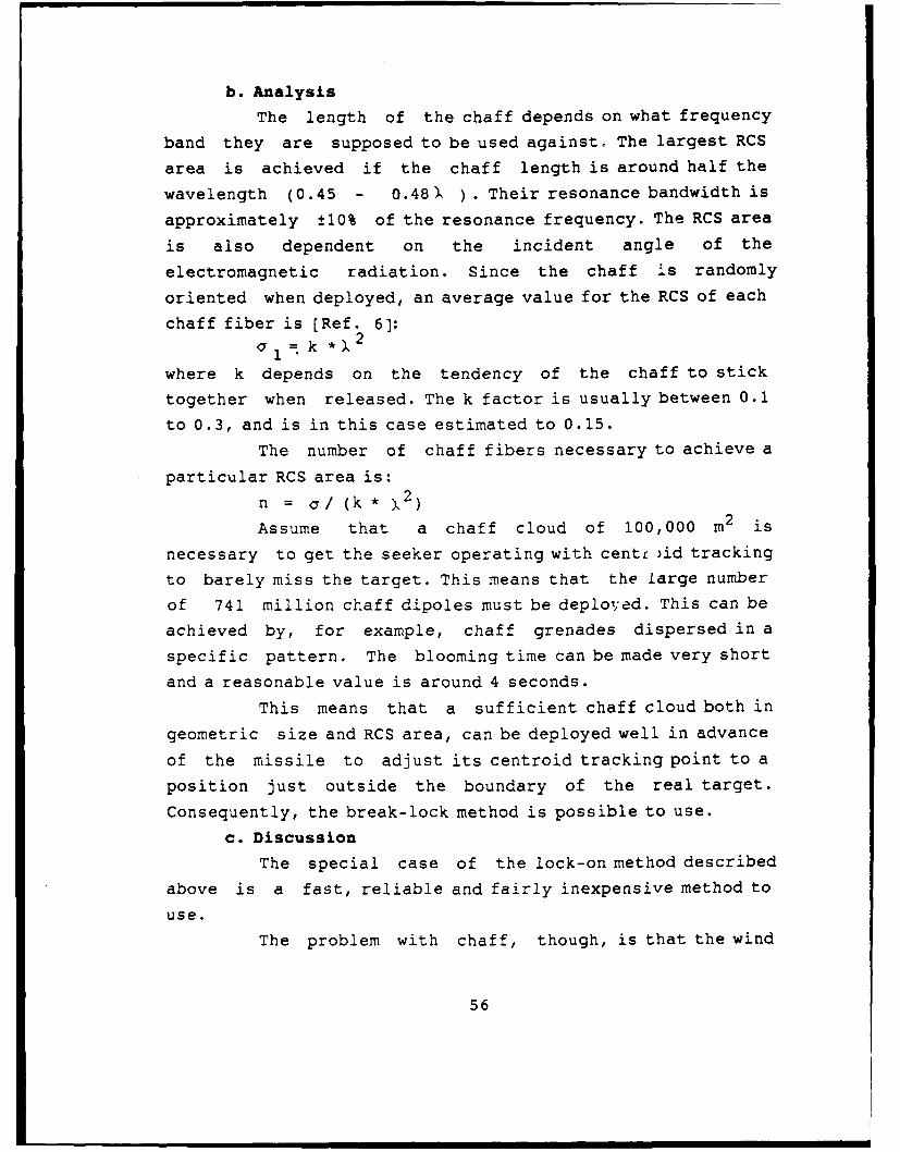
b. Analysis

The length of the chaff depends on what frequency

band they are supposed to be used against. The largest RCS

area is achieved if the chaff length is around half the

wavelength (0.45 - 0.48) ) . Their resonance bandwidth is

approximately ±10% of the resonance frequency. The RCS area

is also dependent on the incident angle of the

electromagnetic radiation. Since the chaff is randomly

oriented when deployed, an average value for the RCS of each

chaff fiber is (Ref. 6]:

1k *

where k depends on the tendency of the chaff to stick

together when released. The k factor is usually between 0.1

to 0.3, and is in this case estimated to 0.15.

The number of chaff fibers necessary to achieve a

particular RCS area is:

n = 7y/ (k * X2)

Assume that a chaff cloud of 100,000 m2 is

necessary to get the seeker operating with centr )id tracking

to barely miss the target. This means that the large number

of 741 million chaff dipoles must be deployed. This can be

achieved by, for example, chaff grenades dispersed in a

specific pattern. The blooming time can be made very short

and a reasonable value is around 4 seconds.

This means that a sufficient chaff cloud both in

geometric size and RCS area, can be deployed well in advance

of the missile to adjust its centroid tracking point to a

position just outside the boundary of the real target.

Consequently, the break-lock method is possible to use.

c. Discussion

The special case of the lock-on method described

above is a fast, reliable and fairly inexpensive method to

use.

The problem with chaff, though, is that the wind

56

direction and velocity have an impact on the effectivenessof the chaff cloud. To counter this, two systems can be

deployed: one in the fore and one in the aft of the ship. It

also accounts for the possibility that the chaff cloud movesin over the target due to the wind. The chaff can be

dispersed by grenades, for example, or some other launching

arrangement. The chaff can be dispersed, taking wind

direction and missile bearing., etc., into consideration.

One chaff grenade might contain chaff for a 100 m2 RCS(Philax system). This means that 1,000 such grenades must be

launched from the fore o- aft each time there is an

indication of a missile tracking radar. This is practically

impossible to pursue since it will be very expensive in bothlaunchers and projectiles and there will be a seriousproblem of reload. Shipborne launchers capable of producing

20,000 m2 clouds per shot exist (NATO SEA GNAT) and

represent an alternative approach.

A considerably smaller RCS area could be acceptableif one considers the same option as in the jammer case,where an impact in an insensitive part of the ship is

acceptable. The fact that the missile seeker prefers a "hotspot" to home on implies that the chaff cloud still must be

significant.

In an effort to reduce the chaff cloud, acombination ECM technique with RGPO, chaff and ship maneuver

can be considered. This technique, however, is based on

ships with relatively high maneuverability and is therefore

not viable in this case.

C. DECOYS

Decoys are mostly thought of as a special kind of

expendable countermeasure used to create false target echoes

or to enhance the signature of a low value target. Decoys

can be deployed by remotely piloted vehicles or simply

launched from the ship. [Ref. 22]

57

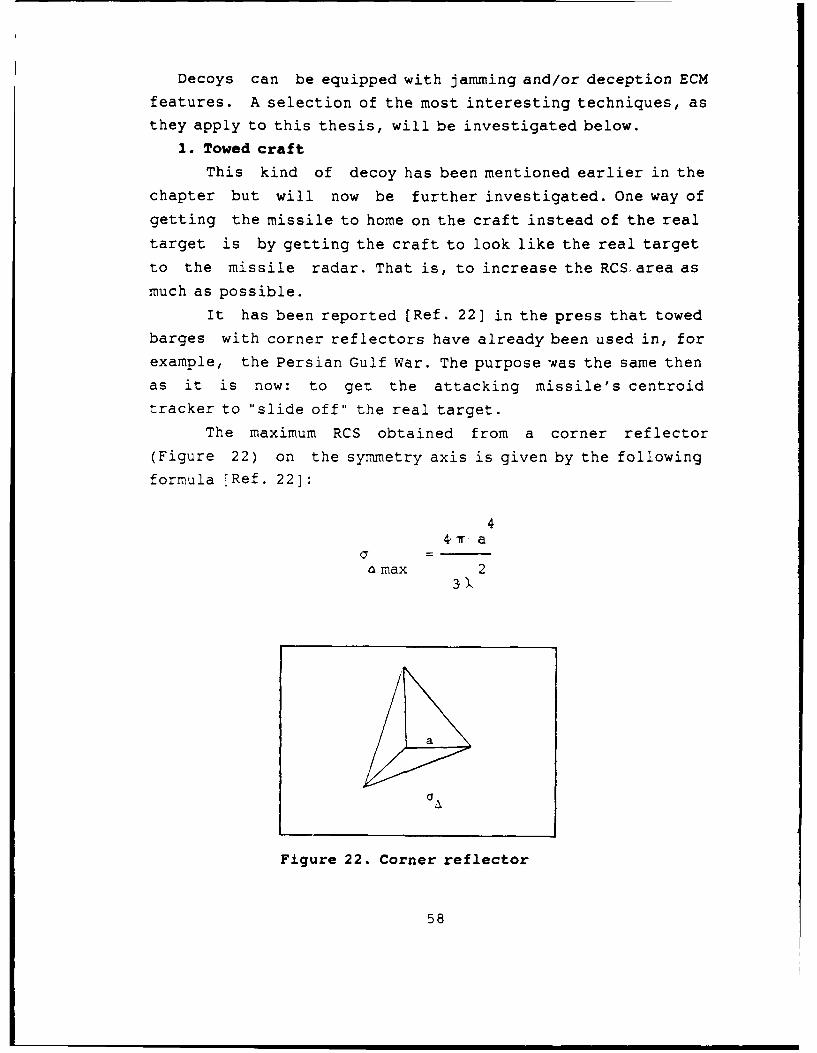
Decoys can be equipped with jamming and/or deception ECM

features. A selection of the most interesting techniques, as

they apply to this thesis, will be investigated below.

1. Towed craft

This kind of decoy has been mentioned earlier in the

chapter but will now be further investigated. One way of

getting the missile to home on the craft instead of the real

target is by getting the craft to look like the real target

to the missile radar. That is, to increase the RCS. area as

much as possible.

It has been reported [Ref. 22] in the press that towed

barges with corner reflectors have already been used in, for

example, the Persian Gulf War. The purpose was the same then

as it is now: to get the attacking missile's centroid

tracker to "slide off" the real target.

The maximum RCS obtained from a corner reflector

(Figure 22) on the symmetry axis is given by the followingformula [Ref. 22]:

44w a

amax 23a

Figure 22. Corner reflector

58

A corner reflector with a side (a) equal to 2.1m gives

an RCS of around 90,000 m2 (around its symmetry axis).

Consequently, a number of corner reflectors would easily

achieve a sufficient RCS area to exceed the real target RCS.

There seem to be both practical and electronic problems with

this approach. Although there are no directly accessible

reports available, some problems can be assumed based on

shiphandling experience. For example, the huge corner

reflectors mounted on the barge deck act like sails, making

the barge very wind sensitive and unstable. Even with

different kinds of anchors to keep the barge in position,

there will still be many problems. This has the consequence

that the ship has very little influence on where the barge

is positioned when the missile is attacking. This is not

satisfactory for the ship commander.

Instead of a corner reflector, one can use Luneberg

lenses. The formula for RCS is given by the formula [Ref. 6]:

3 4-r d

max 4 2

where d is the diameter of the lens.

To get the same RCS area as above, a Luneberg lens of

1.8 m in diameter is required. This will take care of some

of the "sail" effect discussed above, but there is another

problem with Luneberg lenses. They must be kept quite clean

from salt and other particles if their high performance is

to be maintained. They are also much more costly.

Another alternative is to put a deception jammer or a

repeater jammer on the barge instead. This has been

discussed previously and gives both a sufficient simulated

RCS area and is also a more practical solution due to the

59

environment. Probably the best solution is a combination ofcorner reflectors and some kind of jammer, but then theproblem with the large reflectors remains.

The advantages with utilizing a towed craft are:* No power limitations if supplied from the ship.

* The craft is easy to launch when transiting a warzone.

* The distance between the craft and the towing ship iseasy to adjust to get maximum "slide off" effect bythe missile tracker. This must be considered togetherwith shiphandling matters like the tow line, weight,etc.

* The raft is operational until it is hit.

* The corner reflectors can be replaced with smallerLuneberg lenses.

* The detection distance of the missile can be veryshort because of the fact that the decpy is alreadyin position and it is just a matter of directing thejamming device (if not omni-directional) and turn iton.

* Inexpensive technique, since the craft is not wasteduntil the missile hits the craft (missile centroidingextends the craft's lifetime).

The disadvantages are:* The craft can be very wind and sea state dependent,

especially if huge corner reflectors are being used.* Problem with maintaining high performance with

Luneberg lenses close to the water surface.* There might be a problem if the missile is

approaching within 450 of the bow of the ship andthere is not enough time to maneuver.

* If there is an option (not possible in the referencemissile) for the missile launching platform to choosebetween centroid trackinq or left/right edgetracking, once the ECM technique with craft is known,it is easy to change the tracking mode as a countercountermeasure.

* The missile launching tactics can easily be adaptedto the new situation by changing the launchdirection.

2. Buoys

Expendable buoys equipped with a repeater jammer arecurrently under development by contractors in the United

States. These consist of a floating device with a jammer

60

mounted on top. A number of buoys are launched when a threatappears and they immediately start to enhance and repeatincoming signals while in the water. When the batteries aredischarged, they self scuttle and sink to the bottom.

Since the buoy is very small compared to the craftdiscussed above, sea state is an additional environmentalfactor to consider. For example, there can be a signal

direction problem due to high wave crests.

The advantages of buoys are:* Buoys can be easily and quickly launched from the

ship.* Individual buoys are inexpensive, but if the threat

duration is long, the costs can be high.* A number of buoys can be used to simulate false

echoes in the missile search mode.

The disadvantages with buoys are:* The missile intercept and warning must be long enough

to give the target enough time to launch and activatethe uoys.

* As mentioned above, it might be an expensivesolution.

* Tactical placement relative to threat and target isimportant.

3. Rocket decoy

A rocket decoy comprises a rocket with a repeaterjairz-er. The rocket is launched from the ship in a relatively

high elevation angle. When the highest altitude is reached,a parachute is unfolded and while the rocket is slowlydescending toward the ocean surface, the repeater jammer isactive and hence, acts as a false-target decoy. Figure 23shows the "Siren" rocket decoy developed by Marconi Defence

System in the United Kingdom [Ref. 23].The rocket decoy alternative is very similar to the

previously discussed buoy alternative. The major differenceis that the rocket decoy is very wind sensitive and that theoperating time is limited to the time duration of descent.The wind factor is particularly significant in this case

61

340

Figure 23. The "Siren" rocket decoy

since the wind speed and direction varies with altitude. Thedecoy behavior after being launched is therefore very

unpredictable.4. Remotely piloted vehicles (RPV)

A small radio controlled drone can be used as an RPV.

It can be launched from the ship deck and after the missionis completed, land in the ocean to be recovered by the crew.After recovery, it can be cleaned up and prepared for the

next mission. With a number of drones aboard at least onecan be in the air continuously while the ship is transiting

a hostile area.

A drone can measure around 3-4 m in length and bepropelled by a jet engine or an ordinary propeller engine.

Each drone can carry a ECM payload of say 15 kg.

62

The RCS area of the drone itself is very small, from

0.01 m seen from the nose and the tail, to 10 m from each

broadside. [Ref. 23)

The uses of drones are as follows:* Carry radar beacons .(expendable or mounted on the

drone) to deceive the missile radar in search mode.* Disperse chaff for deception, lock-on or break-lock

purposes. This is not a viable alternative in thiscase thouqh since the payload must be very big tosimulate 100 ,oo s RCS area.

* Carry jammer (noise) in applications discussedearlier in this chapter.

The advantages are:The drone can be operating far from the ship and canbe moved quickly to an optimum location.Different kinds of ECM can be loaded into the drone,depending on the situation.

The disadvantages are:

* The payload (15 kg) is very small.

* A special organization is needed aboard the ship totake care of tHe drone.

* Special guiding equipment is needed.

* It is a very expensive system.

D. TACTICS ECM

Tactics ECM is a matter of what the ship commander can

do with the ship in an effort to deceive the missile and/or

combine ship tactics with other ECM.

The most viable tactic in this case is to use shipmaneuvers in combination with another ECM. This has been

discussed in the chapter above.

One way to "hide, the ship using only ship tactics is to

operate the ship so closely to the coast that the coast line

and the ship itself is within the seeker's resolution cell.

However, this tactic is terrain and navigation dependent.

63

One obvious consideration for the ship commander is, ofcourse, to choose the less hostile transiting path throughthe war zone. This includes collecting information about

hostile forces and missile batteries ashore, etc.

E. ECM CONCLUSIONS

All of the ECM support techniques described above aremore or less possible to pursue. This section of the chapterwill decide which technique or combination of techniques isthe most viable against the reference missile. To do this,

the expected performance criteria will be defined and thencompared to the available techniques. The technique(s)selected will provide a new set of options to be evaluated

in a similar manner. The evaluation will be done in four

levels:* Very high

* High

* Medium

* Low

Comments will be made for each choice of level.The evaluation is the author's own judgement and is based

on theoretical guidelines and naval experience since noperformance data is readily available.

The following is a list of performance criteria given inpriority order:

Operational effectiveness. This will answer the overallquestion: "Over a given period of time, how well does thealternative achieve the objective of protecting the shipfrom a missile attack?" (Ref. 24] The period of time is in

this case the time the ship is spending in the "war zone."

Risk. This is the risk that vital parts of the ship,including the crew, will be influenced by the missile

impact.

64

Life-cycle cost. This will include:* research and development cost* production and construction cost

* operation and support cost (like personnel and ESMsupport)

Reliability. The reliability can be defined as theprobability that the alternative will perform when needed."When" is, again, during the war zone transit. Otherconsiderations include:

* geographic location of the war zone* day and/or night capability

* weather and sea conditions

Supportability. The suppcrtability includes the following

issues:* number of personnel needed to maintain a developed

system* education level of the operating personnel

* training of personnel

* human factors

Transportability. The transportability will includeissues like:

* size and weight

* ease of installation and removal

The main ECM alternatives discussed in the chapter arelisted below. The alternatives are not entirely comparablebut this approach will simplify the decision process.Combining techniques will be discussed when appropriate.

A. Selfscreen noise jamming (from the ship itself)B. Deception jamming, RGPO from the ship

C. Chaff in a lock-on methodD. Decoys (includes using part of the ship as a decoy)E. Radar Absorbing Materials (RAM)

65

Alternative A will be excluded from the decision process

since this is not a viable alternative due to the reference

missile being equipped with HOJ capability.

Details are shown in Tables 7, 8, 9, 10.

TABLE 7. EVALUATION OF SELFSCREENING REPEATER JAMING

Crite'ia Ealation Comments

LeveL

Operational eflectiveness Meci.m Positive: * The same jammer can be used all

the time through the war zone

* Effective against radars with no

human operator involved

* Manage to deceive more than one

incoming missile

Negative: * With only RGPO the reacquisition

time can be very short

* The jammer can be saturated byother transmitters

* Doubtful technique since the

boresight is aimed at the target

Risk High Negative: * The jammer is located aboa-d the

ship

Life-cycle cost Lo- Positive: * State of the art technique

* Inexpens've system to operate and

support

Reliability H'gM Positive: * The technique has been tested and

oparable for many years

Supportability High Positive: * The system can be operated

autonomously

Transportability High Positive: * Low size and weight

66

TABLE 8. EVALUATION OF CHAFF IN LOCK-ON METHOD

Cr'te'ia Evaluation Commentslevel

Medium Positive: * Chaff can be made for broadOperational effectiveness bandwidth

* Manage to deceive more than oneincoming missile

• Easy to combine with other ECMtechnique

• Very good historical experiencewith chaff

Negative: * Practical problems to achievesufficient RCS area for thereference target

* Probiems to reload and aidlaunchers

* Needs relatively long warningtime

Risk eoum Negative: * Chaff cloud is dispesed close tothe ship itself

Life-cyc~e cost Me>' rim Posit'e: * State of the art technique* Chaff grenades themselves

relatively inexpensiveNegative: * Launching technique can be

expensi ie* The chaff technique will be

expensi.e if many "false alarms"and long transition distance forthe ship

ReLiabLity mea, Posit,,e: * Well established technique

Negati e: * Chaff fibers can bundle together

* Chaff is sensitive to wind in

comb'nation with the ship heading

Supportabilaty Medium Negative: * Need a special organizationaboard for reloading thelaunchers, etc.

Transpcrtability LO. Negative: * The amount of chaff grenades that

are needed together withlaunching equipment that must bemounted and aligned in differentpattern, etc., makes thetransportability low.

67

TABLE 9. EVALUATION OF DECOYS

Criteria EvaLuation Comments:

Level

Operational effectiveness Medium Positive: * Can in some cases use combined

ECM techniques

Negative: * UsuaLly power Limitations

* UsualLy warning time necessary

Risk Low Positive: * UsualLy decoy depLoyed far from

vitaL parts of the ship

Life-cycle cost Medium EvaLuation depends on the technique chosen

to high

ReLiabiLity Medium Negative: * Decoys can be (very) sensitive to

weather and sea condition

Supportability Medium Evaluation depends on the technique chosen

Transportability Medium Evaluation depends on the technique chosen

TABLE 10. EVALUATION OF RADAR ABSORBING MATERIAL

Criteria Evaluation Comments

Level

Operational e'fecti.eness Mec'um Positive: * No warning time necessary

Negative: * LimiteC bandwidth

Risk Meoaum Negative: * Even if the abscrbing efficiency

is high, the large ship size can,

despite this, give a significant

RCS area

Life-cycle cost High

ReLiabiLity High

Supportab'lity N/A

TransportabiLity N/A

68

Alternative D is also divided into different kinds of

decoys. They are:

A. jammer aboard spec prepared ship section (JS)

B. towed craft

C. buoy

D. rocket

E. rpv (drone)

The decision process continues further (Tables 11, 12,

13, 14, 15) with the same criteria definitions areas

previously outlined.

TABLE 11. EVALUATION OF JAMMER

Criteria EvaLuaaion Commets

LeveL

Operational effectieness High Positive: * Easy for the seeker to change to

new "hot spot" on the ship* No power Limitations

Risk High Negative: * The missile is deLiberately

guided to the ship (close to the

crew and other vital parts)

Life-cycle cost Lo-

Reliability High

Supportability High Positive: * The system can be made autonomous

Transpo-tabiLity High Negative: * Needs certain preparations aboard

69

TABLE 12. EVALUATION OF TOWED CRAFT

Criteria Evaluation Comments

level

Operational effectiveness High Positive: * No warning time necessary

* Easy to use combined ECM support

* No power Limitations

* Craft is operable until destroyed

by missile impact

Negative: * Easy to make tactical adaption by

the hostile force

Risk Low Decoy is separated from ship

Life-c 7Le cost Low

Re Liabl ity Low

Supportability Meaium Negative: * Weather and sea sensitive

* Maneuverability problem

Tra:isportabdiLty High Need personnel for Launching, etc.

TABLE 13. EVALUATION OF BUOY

Criteia EvaLuation lomme-tslevel

OperationaL effeztveness Meo uLm Positive: * Easy to use tactically

Negative: * Too small for combined ECM

• Power limited

* Warning time necessary

Risk Low to Dependent on warning time

Medium

Life-cycle cost Medium Buoys expandable

Reliability Medium Can be sea-state sensitive

Supportab'lity High Can be made autonomous

Transportablity High

70

TABLE 14. EVALUATION OF ROCKET

Cr ,ter ia EvaLuation CommentsLeveL

operationaL effectieness Medium Positive: * Easy to use tacticaLLYNegative: * Too smaLL for combined ECM

* Power Limited* Warning time necessary

* Radar co,;erage prooLem

RiSK Low to Dependent on warning timemed i um

Life-cyc~e cost Meo!ium Decoy expendabLe

ReLiab'Lity Med i im Wind sensitive

SuppcrtabiLity H' 91" Can be made autonomous

Transportanit Hig

TABLE 15. EVALUATION OF REMOTE PILOTED VEHICLE

Cr'teia EvaLuation Comme-ts

Levet

OperaticraL e4fect .e-ess me!' , ~ Negati~e: * Needs warning time

* Limited pay-Load and poier

Risk .o toMeti jm

L-,fe-cvc~le cost ve-y Higr. RPV is a sopr'st':ated decoy

ReLiab' L'ty !ledvr weather dependent

Sup~otan~tity Lot. Needs special. y-tra'ned pe-sonnel for both

Launching, maintenance and operation

Transportabi L'ty e'J

71

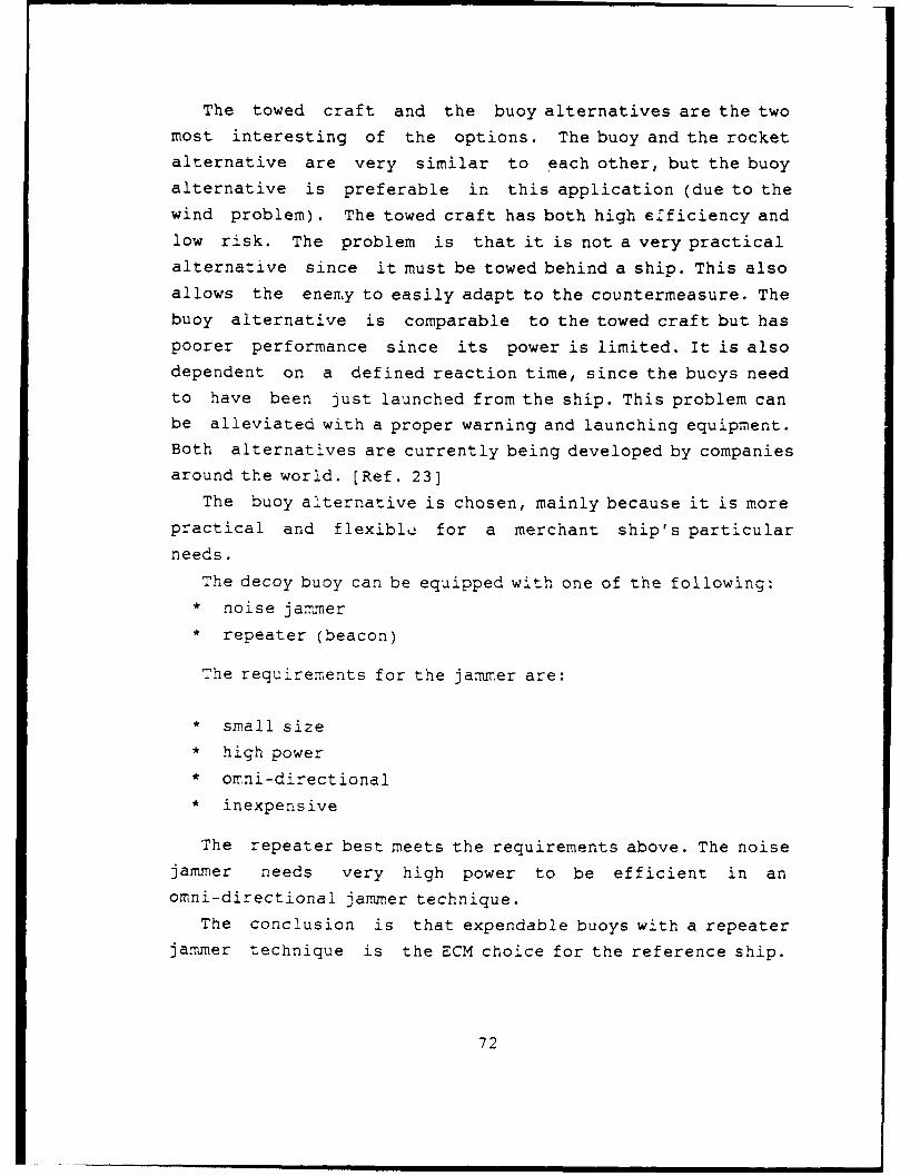
The towed craft and the buoy alternatives are the twomost interesting of the options. The buoy and the rocketalternative are very similar to each other, but the buoyalternative is preferable in this application (due to thewind problem). The towed craft has both high efficiency andlow risk. The problem is that it is not a very practicalalternative since it must be towed behind a ship. This alsoallows the enenmy to easily adapt to the countermeasure. Thebuoy alternative is comparable to the towed craft but haspoorer performance since its power is limited. It is alsodependent on a defined reaction time, since the buoys need

to have been just launched from the ship. This problem canbe alleviated with a proper warning and launching equipment.Both alternatives are currently being developed by companiesaround the world. [Ref. 23]

The buoy alternative is chosen, mainly because it is morepractical and flexiblQ for a merchant ship's particular

needs.

The decoy buoy can be equipped with one of the following:* noise jarnmer

" repeater (beacon)

The requirements for the jammer are:

" small size

" high power

" omni-directional

" inexpensive

The repeater best meets the requirements above. The noisejammer needs very high power to be efficient in anomni-directionai jammer technique.

The conclusion is that expendable buoys with a repeaterjammer technique is the ECM choice for the reference ship.

72

The buoys should be launched autonomously in predetermined

directions. The warning must be early enough to give the

activated buoys time to be effective against the missile.

73

V. ECM RECOMMENDATIONS

Given the discussion above, the most appropriate ECM

support for the reference tanker is the expendable,

omni-directional, repeater jammer buoy.

This chapter will expand the buoy alternative further and

discuss the kind of support requirements needed. The chapter

will not include buoy patterns and other tactical

considerations.

The general requirements for an operable buoy ECM system

are as follows:* the system must be easily installed and removed

* the system must be nearly autonomous, or if not, veryuser friendly

* the buoys must be launched to at least a few hundredmeters from the ship in any direction.

* the buoys must be activated within 30 sec (10 km)from the first detection of the missile and stayactive for at least two minutes.

The following topics will be covered in the chapter:* repeater jammer operational characteristics

* general buoy description

* ESM support

A. REPEATER JAMMER

The objective of the repeater jammer is to create a

credible false target close to the ship in order to deceive

the missile seeker. Given the specifications discussed

earlier, a repeater jammer can be made small (dimensions)

and light (weight) as mentioned in Chapter 3.

74

To create a credible false target, the jammer must repeat

an incoming signal that corresponds to 100,000 sm RCS area.

The following calculations will determine the necessarysystem gain and power requirements.

For unity J/S ratio, the required system gain is given by

[Ref. 23]:

G = 1.4 * 104 * A (F)2

where A is the target cross section in square meters and F

is the operating frequency in Megahertz.

This gives for A = 100,000 sm and F = 10 GHz a required

gain of approximately 90 dB.

For unity J/S ratio and an omni-directional jammingantenna the required "electronic" power output is given by

(Ref. 23]:

P G ct t

P =

j 24w R-f j

where Pt = output power in watts (radar)Gt = antenna power gain (radar)

This gives (Pt = 30 KW, = 100,000 sm and Gt 27 dB

in the mainlobe) the ranges shown in Table 16.

This shows that the earlier the jammer buoys are launchedand activated, the less power is required to simulate afalse target with 100,000 sm RCS area. On the other hand, inorder to deny the missile the ability tc change target from

the buoy to the ship during its approach, the jammer must

keep the high RCS return to a very close distance, which

implies the need for the very high output peak power

requirements calculated above. This will also assure thatthe missile target seeker will initially "lock on" the buoy.

75

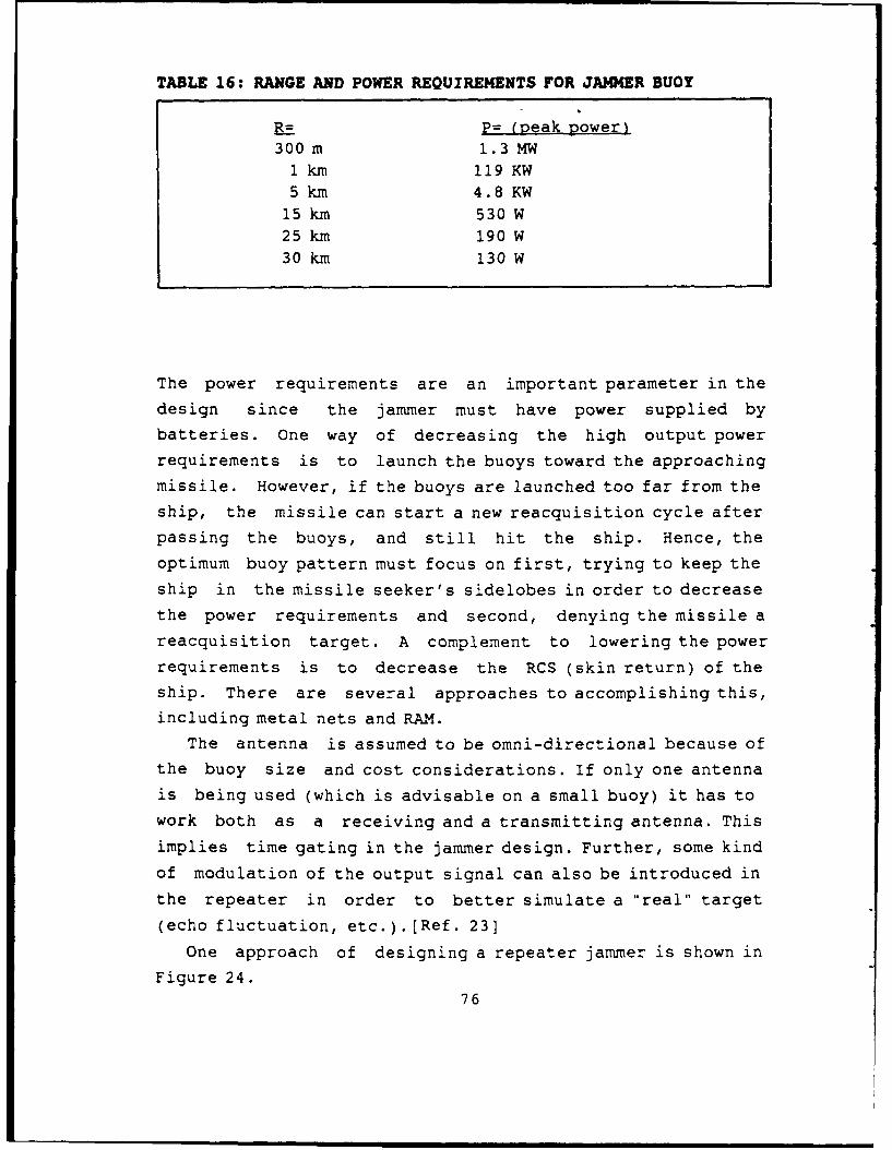
TABLE 16: RANGE AND POWER REQUIREMENTS FOR JAMMER BUOY

R= P= (peak power)300 m 1.3MW1 km 119 KW5 km 4.8 KW15 km 530 W25km 190 W30 km 130 W

The power requirements are an important parameter in the

design since the jammer must have power supplied by

batteries. One way of decreasing the high output power

requirements is to launch the buoys toward the approachingmissile. However, if the buoys are launched too far from the

ship, the missile can start a new reacquisition cycle after

passing the buoys, and still hit the ship. Hence, the

optimum buoy pattern must focus on first, trying to keep the

ship in the missile seeker's sidelobes in order to decrease

the power requirements and second, denying the missile a

reacquisition target. A complement to lowering the power

requirements is to decrease the RCS (skin return) of the

ship. There are several approaches to accomplishing this,

including metal nets and RAM.

The antenna is assumed to be omni-directional because of

the buoy size and cost considerations. If only one antenna

is being used (which is advisable on a small buoy) it has towork both as a receiving and a transmitting antenna. This

implies time gating in the jammer design. Further, some kind

of modulation of the output signal can also be introduced in

the repeater in order to better simulate a "real" target

(echo fluctuation, etc.). [Ref. 23]

One approach of designing a repeater jammer is shown in

Figure 24.76

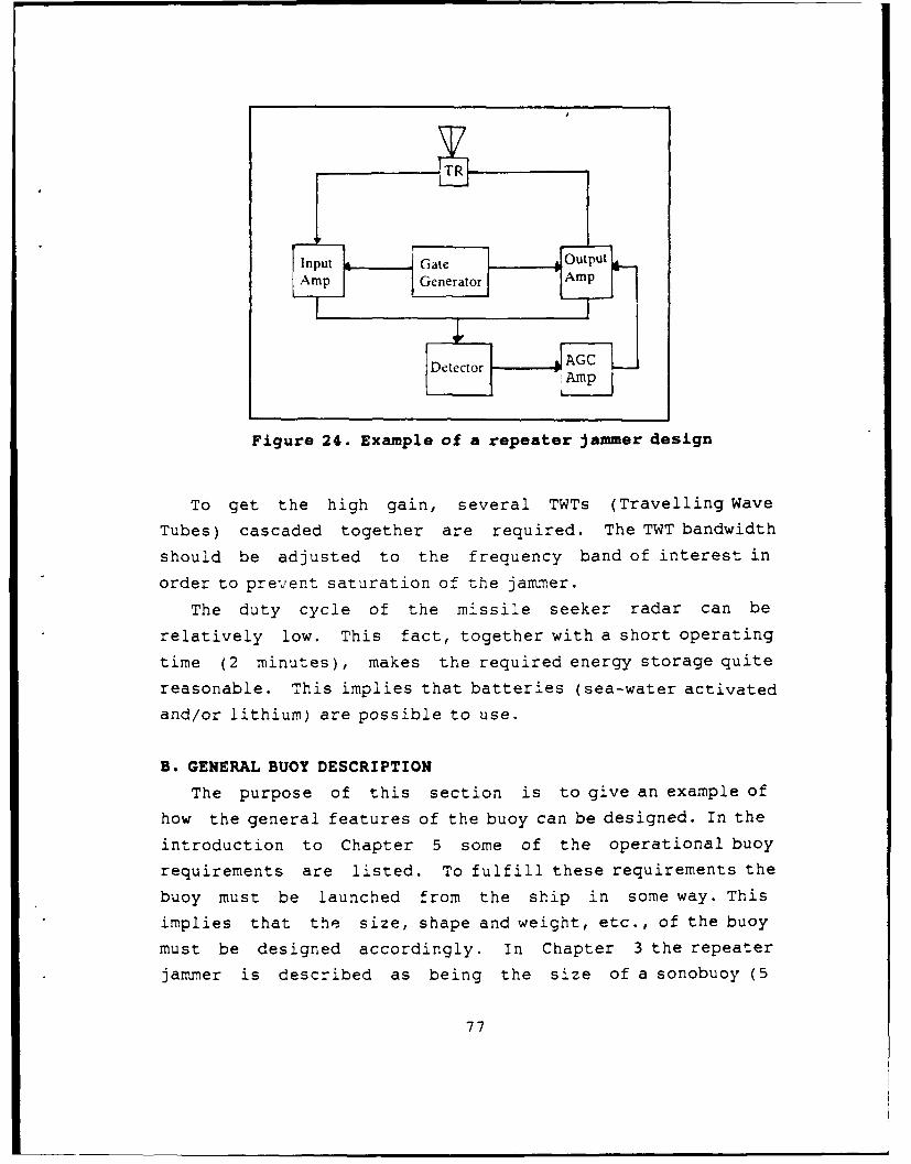
IptGate O u

Arm GeneratorAm

Detector

Figure 24. Example of a repeater jammer design

To get the high gain, several TWTs (Travelling Wave

Tubes) cascaded together are required. The TWT bandwidth

should be adjusted to the frequency band of interest in

order to prevent saturation of the jammer.

The duty cycle of the missile seeker radar can be

relatively low. This fact, together with a short operating

time (2 minutes), makes the required energy storage quite

reasonable. This implies that batteries (sea-water activated

and/or lithium) are possible to use.

B. GENERAL BUOY DESCRIPTION

The purpose of this section is to give an example of

how the general features of the buoy can be designed. In the

introduction to Chapter 5 some of the operational buoy

requirements are listed. To fulfill these requirements the

buoy must be launched from the ship in some way. This

implies that the size, shape and weight, etc., of the buoy

must be designed accordingly. In Chapter 3 the repeater

jammer is described as being the size of a sonobuoy (5

77

inches in diameter, 30 inches long). Why not use the

well-developed and thoroughly-tested sonobuoy concept andadapt that idea here? This leads to the following general

buoy philosophy:

The buoy(s) should be delivered folded aboard the ship insome kind of container, ready to be launched. The containers

should be mounted on the ship deck in such a way as to cover

a number of launching bearings from the ship.

When the buoy is launched from the ship and hits thewater surface, it should unfold itself and begin jammingimmediately. After the active phase (i.e., when thebatteries are out of energy) the buoy should lose itsbuoyancy and sink to the sea bottom.

The deployed unfolded buoy is depicted in Figure 25.

[Ref. 26]

Taking advantage of proven techniques keeps thelife-cycle cost of the system down. Also, many otherrequirements, such as the supportability andtransportability questions, etc., would already be

satisfied.

There are two launching technique options: 1. using arocket to deliver the buoy in position, or 2. using somekind of catapult. There are advantages and disadvantageswith both of these techniques. The rocket can deliver the

buoy faster and to a greater distance from the ship than the

catapult. On the other hand, the catapult technique giveslower acceleration stress and is much safer to handle.

Tactical considerations will determine the most applicable

technique.

C. ESM SUPPORT

In order to launch the buoy in time to be effective,sufficient warning of an incoming missile is needed. Thiscan be accomplished in from one to three ways: optically,

radar or ESM. The ESM way is probably the most reliable

78

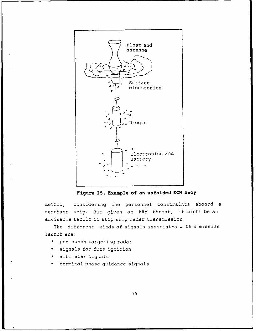
Float and

antenna

00tSurface

a° electronics

d

.4 Drogue

- Electronics ando Battery

Figure 25. Example of an unfolded ECM buoy

method, considering the personnel constraints aboard a

merchant ship. But given an ARM threat, it might be an

advisable tactic to stop ship radar transmission.

The different kinds of signals associated with a missile

launch are:* prelaunch targeting radar

* signals for fuze ignition

* altimeter signals

* terminal phase guidance signals

79

L

To receive as much warning time as possible, the most

viable alternative appears to be detecting the signals

radiated from the missile in its terminal phase and signals

from prelaunch targeting radar. The detection of the signals

radiated from the missile in its terminal phase is estimated

to be the most important and least ambiguous.

The following ESM issues will be treated:* signal environment

* receiver

* signal processing

* user interface

The general requirements for the ESM system are:

* Real time operation. The threat missile must beintercepted, detected and classified as soon as itstarts radiating.

* Omni-directional coverage. The assumption is thatwhile there may be a preferred direction of attack,the system must be designed for attacks originatingfrom any direction.Easy to operate. The system would be operated bynon-military people who probably would not spend muchresources on training to use the system. As such, thesystem must be easy to operate with minimal training.

This translates into a requirement for a high degreeof automation.Relatively inexpensive system.

The main objective for the receiver is to intercept and

determine the lethality of incoming signals as quickly as

possible.

Since the threat in this case is something quite

specific, one design approach for making the system response

faster would be to filter out unwanted signals as early as

possible, in order to keep low the amount of data that needs

to be processed.

80

The mode of operation would be to let the system receive

signals from the environment and search for the specific

missile threats -hat the operator deems to be significant

for the particular war zone through which the ship is

transiting. After having detected and classified the threat

missile, it would alert the operator and pass threat

information to some kind of ECM processor that computes

launching data for the buoys and also issues maneuvering

recommendations to the bridge operator to increase the

probability of countering the threat successfully.

1. Signal environment

The assumption is that the emitters in the

environment, in the frequency band of interest, are from

civilian or military ships and coastal radars. A pulse

density of about 90,000 pulses per second is estimated from

assumptions about the maximum PRF arising from unambiguous

range requirements. (See Appendix H)

The merchant ship itself will have its own

transmitters that may, because of the short distances

involved, get into the ESM system. These signals have to be

screened out to prevent false alarms.

2. ESM receiver

The receiver in this ESM system must be some kind of

Radar Warning Receiver (RWR). An RWR is characterized as a

simple, rugged and relatively inexpensive receiver. A simple

RWR system block diagram is shown in Figure 26 [Ref. 6].

There can be a number of integrated antennas and

receivers to cover all azimuth angels and frequency bands.

The performance of an RWR is usually discussed in

terms of sensitivity, dynamic range, probability of

intercept (POI) and throughput rate.

Short definitions of the different terms are given

below. [Ref. 27]

The sensitivity of a receiver is a function of the

ratio of RF bandwidth and video bandwidth.

81

Criteria

I I Alarm

Antenna Receiver Analysis

Figure 26. Simple RWR block diagram

The dynamic rakngf is used to indicate the input sicnal

amplitude range that the receiver can process properly. The

lower limit of the dynamic range is the sensitivity of the

receiver.

The POI is used to tell the percentage of pulses the

receiver will collect in a certain signal environment.

The throughput rate is applicable when the signals are

pulsed and tells the maximum pulse rate the receiver can

process.

One important missile seeker parameter to be

determined by the RWR is the antenna scan pattern. The fact

that the missile seeker is scanning in a sector, which means

that the dwell time on the target is relatively long, makes

this parameter very significant.

Other significant parameters are Angle Of Arrival

(AOA), Pulse Repetition Interval (PRI), Pulse Width (PW),

Frequency and Signal Amplitude.

The following discussion about the required

performance parameters for the receiver can be made:

* The receiver sensitivity need not be extremely highsince the seeker radar is quite powerful and thedistances considered are relatively sho. S - 30km).

82

I I II • I I I I Ii

* The receiver must have wide dynamic range to be ableto handle both strong and weak signals.

* The probability of intercept must be as high aspossible.The different kinds of RWR receivers (state of the

art) that can be considered are:* the crystal video receiver

* the instantaneous frequency receiver (IFM)

* the superheterodyne receiver

* the wideband YIG-tuned superheterodyne receiverThe most important features of the techniques are

summarized below.

RWR often use a crystal video receiver, which means

that the mixer, local oscillator (LO) and the IF amplifier

are missing. A block diagram of the receiver is shown in

Figure 27 [Ref. 18].

Comp,...

NF AwfI@1 V id

uit..Z~v"'~~SandH'- Sa1

>7/ BoSnd 2

Figure 27. The crystalvi eo receiver

The receiver is relatively simple, low in cost,

lightweight and small in size. It is used for wideband

detection (2 - 18 GHz) of low duty cycle signals but can

also be modified for CW detection.

The disadvantage with the receiver is that it cannot

closely determine the frequency of the incoming signal.

83

Another disadvantage is that the key threat signals can be

masked by other signals and noise jamming.

The sensitivity of the receiver is relatively low,

between -50 dBm and -60 dBm. It has a high probability of

intercept and a large dynamic range.

The IFM receiver is essentially a crystal video

receiver but is provided with a delay line which makes it

possible to measure frequency. The RF bandwidth is wide,

sometimes up to more than one octave. The weakest point in

the IFM receiver is that it can be captured by a strong CW

or jamming signal. There are ways of getting around this

problem, [Ref. 27] by using a frequency rejection technique

for the offending emitter. The POI can be made to approach

100%. The dynamic range and the sensitivity are moderately

high.

Modern IFM receivers are mostly digitized (DIFM),

which gives the ability to detect intrapulse frequency agile

emitters. Some typical DIFM values for X-band interception

are a sensitivity of -65 dBm and a dynamic range of 70 dB.

A typical block diagram of an IFM receiver is shown in

Figure 28 [Ref. 18]. IFM/DIFM receivers are mostly used in

SIGINT applications.

Figure 28. The IFM receiver

A superheterodyne receiver has a very high

sensitivity, excellent selectivity and frequency resolution.

Superheterodyne receivers use a mixer, LO and filter to get

84

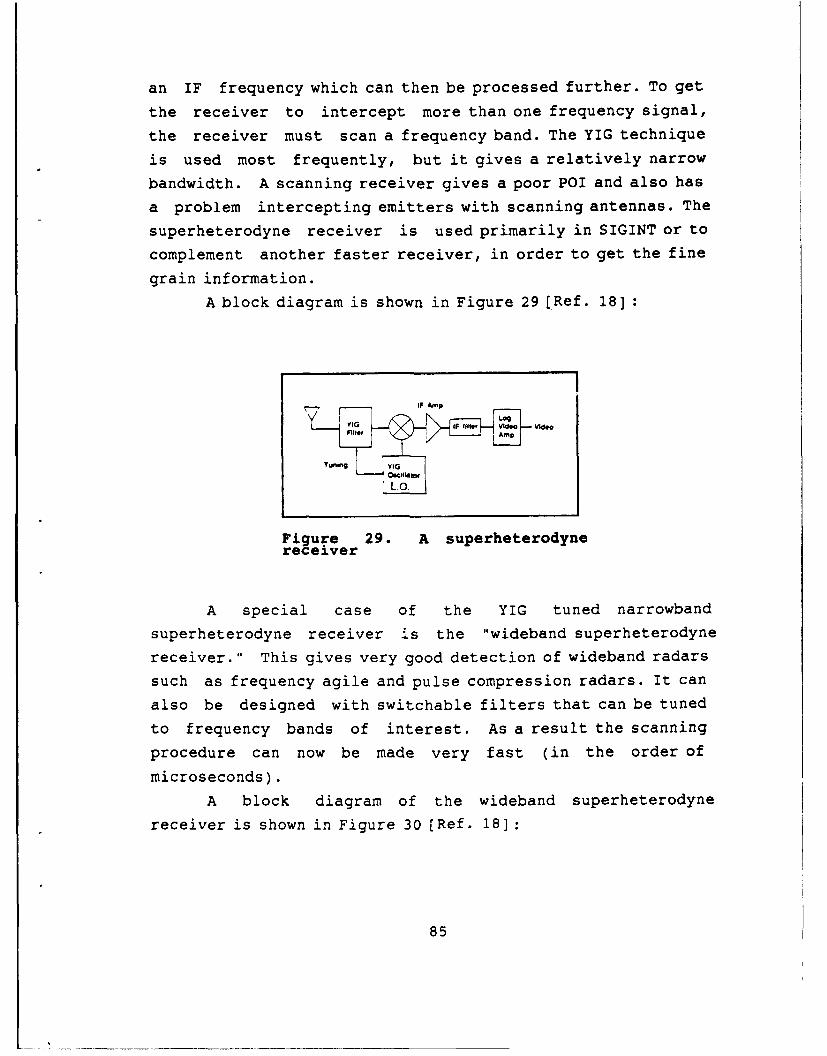
an IF frequency which can then be processed further. To get

the receiver to intercept more than one frequency signal,

the receiver must scan a frequency band. The YIG technique

is used most frequently, but it gives a relatively narrow

bandwidth. A scanning receiver gives a poor POI and also has

a problem intercepting emitters with scanning antennas. The

superheterodyne receiver is used primarily in SIGINT or to

complement another faster receiver, in order to get the fine

grain information.

A block diagram is shown in Figure 29 (Ref. 18]

Figure 29. A superheterodynereceiver

A special case of the YIG tuned narrowband

superheterodyne receiver is the "wideband superheterodyne

receiver." This gives very good detection of wideband radars

such as frequency agile and pulse compression radars. It can

also be designed with switchable filters that can be tuned

to frequency bands of interest. As a result the scanning

procedure can now be made very fast (in the order of

microseconds).

A block diagram of the wideband superheterodyne

receiver is shown in Figure 30 [Ref. 18]

85

Filter IF Filter TamjedRSignal

fast tuning LO

Figure 30. The widebandsuperheterodyne receiver

As indicated above, the most common receiver in RWRapplications is the Crystal Video Receiver. However, it mustbe complemented with another receiver (i.e., asuperheterodyne receiver) to measure frequency, and thistakes time. Further, the wide bandwidth capacity is not arequirement for the receiver in this application. It is,rather, a disadvantage since only very specific signals in alimited frequency band need to be detected.

Another alternative might be to consider a widebandsuperheterodyne receiver. The receiver would be stepped to aparticular frequency band of interest where it then sweepsthrough this band continuously. It would consequently spendless time scanning, resulting in a higher POI.

In this way unwanted frequencies will be filtered out,since they are outside the band of immediate interest, andthe downstream processing need not cope with these signals,which will speed up the processing rate. The penalty ofusing some kind of scanning receiver is always that the POIgoes down, even though the frequency band is limited and thescanning rate very high.

To fulfill the requirements of AOA, a number ofmatched receivers can be arranged in a certain configuration(i.e., four receivers, one in each quadrant). Theintercepted signal's amplitude and/or phase is then comparedbetween the receivers.

86

3. Signal processing

In order to get high throughput rate, further

filtering can be applied before the actual pulse parameter

measurements in the preprocessor. The main processor could

be in parallel with auxiliary processors. To process the

signals in real time, window addressable memory (WAM) can be

used to assist in the pulse deinterleaving and pulse train

matching. The display console should also be "smart" in

order to off load the main processor. E.g, keyboard scanning

and interpretation should be done by the display console

itself.

4. User interface

In order to be an autonomous system the user interface

must be provided with an automatic mode. When the processor

finds a lethal match, i.e., an incoming missile, launch data

should go directly to the buoy system and to the maneuvering

display, via some kind of "ECM processor." The ECM processor

should calculate the necessary launching and maneuvering

data, due to the ship's RCS variations, maneuvering data and

wind conditions, etc.

Even though the system can be put in an automatic

mode, an operator must be able to manually operate the

system and provide it with necessary initial values. The

user interface can consist of a pictorial display, a numeric

keypad and some hard and soft keys. The soft function keys

can have descriptions written on the display and a menu

selection method can be used for prompting and obtaining

operator commands. The pictorial display must show the

threats (with azimuth and estimated range) and the

maneuvering recommendation.

87

VI. ACOUSTIC ENVIRONMENT STUDY

A. INTRODUCTION

This chapter will give a general description of theBaltic Ocean characteristics and will provide specificdetail of the water volume of interest in the sonar design.

B. THE BALTIC OCEAN

The Baltic Ocean is a sub-sea to the Atlantic Ocean andis delimited by the Scandinavian peninsula and the Danish

Islands (see Appendix I). The area is 366,000 km2 and the

average depth is 65 m. [Ref. 28] The Baltic is in some sensean inland sea, since it has very narrow and shallow

connections to the North Sea and the Atlantic in the west.The water balance can be described with Figure 31 below. Thelarge amount of water from the many rivers makes the Baltica brackish sea, and the salinity can vary considerably

depending on geographical location and depth (Figure 31).

Figure 31 shows that the Baltic works more or less like a

gigantic mouth of a river [Ref. 29].

The sea-bottom conditions vary both in roughness andconsistency, depending on the geographical location. The sea

bottom in the specified water volume will be described later

in this chapter.

The density of water depends on salinity, pressure and

temperature. Low density water is lighter and is layered ontop of high density water. Fresh water supplies from the

rivers, wind and tt,. 1--rature variations help to destroy or

maintain established -° :er layers. How the salinity in the

Baltic varies is shown in Figure 32 [Ref. 29].

88

waterbalance in Kin 3/yearb)70a45

b) from rain

d-e) water exchange Baltic Sea -Kattegatt,

Figure 31. Water balance in the Baltic Sea

Salinity in PPM .4

-

3

Figure 32. Salinity variations inthe Baltic Sea

89

1. SalinitySalinity in the middle of the Baltic is 6.5 - 7.5 PPT,

in a layer from the surface down to 60 - 80 meters depth. Indeep water regions, salinity increases to 10 - 12 PPT.

2. Currents

The sea currents are created and maintained by the

following forces:* wind

* horizontal water density differences

* slope of the sea surface

* tide

* air pressure differences

The wind influences mainly the water closest to thesea surface and the effect decreases rapidly with depth.Water volumes can have different densities which creates

pressure differences and hence, currents. If the watersurface is slanted, this also causes pressure differences.

Tide always implies currents, but sin'e the tide in theBaltic is negligible, the contribution is small. The airpressure forces the sea surface level to go higher and lowerwhich also creates currents. The velocities of the deep sea

currents are shown in Figure 33 [Ref. 29].

Depth Wind (m/s)(M) 1 5 10 20 30

0 0,1 0,2 0,5 1,0 1,5

1 0,0 0,1 0,2 0,4 0,5

5 0,0 0,1 0,1 0,2 0,310 0,0 0,1 0.1 0,2 0,2

15 0,0 0.0 o,1 0,2 0.2

Figure 33. The velocity of the deep seacurrents in the Baltic Sea

90

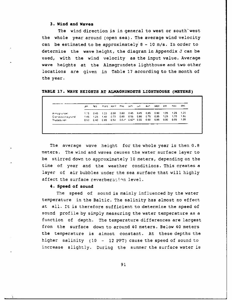
3. Wind and Waves

The wind direction is in general to west or south'west

the whole year around (open sea). The average wind velocity

can be estimated to be approximately 8 - 10 m/s. In order to

determine the wave height, the diagram in Appendix J can be

used, with the wind velocity as the input value. Average

wave heights at the Almagrundets lighthouse and two other

locations are given in Table 17 according to the month of

the year.

TABLE 17. WAVE HEIGHTS AT ALMAGRUNDETS LIGHTHOUSE (METERS)

jan fed rna s apri mal jun. Jul. aur sept 0ok nov dec

Almaq'.nce: 1.15 045 1.3 0.50 0,60 045 0.45 0.65 0.80 1.05 1.25 1.20

COarcs soira rund 1 45 1.25 1.40 0.73 0.60 0.55 0.80 0.75 0.95 1.25 1.70 1.63Trutaoren 0.50 0,40 0,65 0,50 0.E0" 0.60" 0.55 0.60 0,95 0.9C 0.95 1,05

The average wave height for the whole year is then 0.8

meters. The wind and waves causes the water surface layer to

be stirred down to approximately 10 meters, depending on the

time of year and the weather conditions. This creates a

layer of air bubbles under the sea surface that will highly

affect the surface reverberatio, n level.

4. Speed of sound

The speed of sound is mainly influenced by the water

temperature in the Baltic. The salinity has almost no effect

at all. It is therefore sufficient to determine the speed of

sound profile by simply measuring the water temperature as a

function of depth. The temperature differences are largest

from the surface down to around 40 meters. Below 40 meters

the temperature is almost constant. At these depths the

higher salinity (10 - 12 PPT) cause the speed of sound to

increase slightly. During the summer the surface water is

91

warm and the underlying water cold. This implies a sharpnegative gradient and the sound is strongly refracted toward

the bottom. Together with the slightly positive gradient at

deeper depths this creates a sound channel, very much like

the SOFAR channel in the deep oceans. During the winter the

surface water gets colder than the underlying water which

makes the gradient iso-speed or positive. A positive

gradient makes the sound bend toward I ie surface. Further,it is quite normal to have iso-speed water from the surface

and down to 1 - 10 meters due to the stirring effect.

An assumption is that the speed of sound profile is

range independent out to a radius of approximately 1,000

meters. [Ref. 30]

S. Absorption

The absorption of sound in water increases with

frequency and decreases with salinity. The diagram inAppendix K shows the absorption in dB/km vice frequency, for

both the Baltic and the Atlantic ocean. For example, in the

Baltic the absorption is 9 dB/km at 100 KHz compared with 30

dB/Km in the Atlantic Ocean. This means that higher

frequencies are more favorable in the Baltic, which also

implies that smaller and lighter transducer dimensions may

be used.

C. DESCRIPTION OF THE WATER VOLUME

The location of the water volume, that will be the

reference for the sonar design calculations, is shown in

Appendix L. The speed of sound profiles for differentmonths, together with ray tracing results are shown in

Appendix M. The typical sea bottom condition is shown in

Figure 34 [Ref. 31].

92

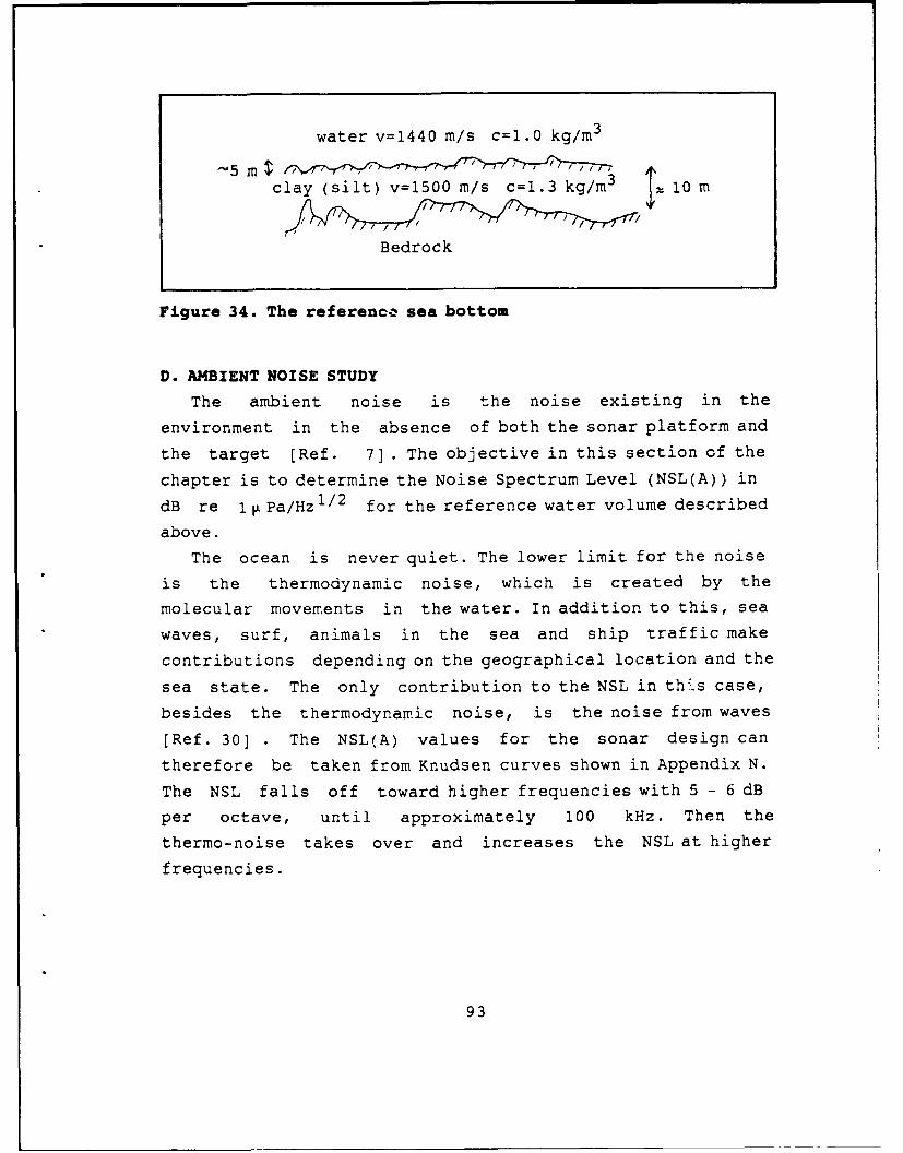
water v=1440 m/s c=1.0 kg/m 3

5 mS T '' I , i

clay (silt) v=1500 m/s c=1.3 kg/m 0 m, Al,

Bedrock

Figure 34. The reference sea bottom

D. AMBIENT NOISE STUDY

The ambient noise is the noise existing in the

environment in the absence of both the sonar platform and

the target [Ref. 7]. The objective in this section of the

chapter is to determine the Noise Spectrum Level (NSL(A)) in

dB re 1 V Pa/Hz 1/2 for the reference water volume described

above.

The ocean is never quiet. The lower limit for the noise

is the thermodynamic noise, which is created by the

molecular movements in the water. In addition to this, sea

waves, surf, animals in the sea and ship traffic make

contributions depending on the geographical location and the

sea state. The only contribution to the NSL in this case,

besides the thermodynamic noise, is the noise from waves

[Ref. 30] . The NSL(A) values for the sonar design can

therefore be taken from Knudsen curves shown in Appendix N.

The NSL falls off toward higher frequencies with 5 - 6 dB

per octave, until approximately 100 kHz. Then the

thermo-noise takes over and increases the NSL at higher

frequencies.

93

VII. SONAR DESIGN STUDY

A. INTRODUCTION

This introduction will determine the sonarspecification and give a more detailed picture of the design

objective. It will also explain the design method that will

be used in pursuing the objective.

As indicated in Chapter 1, the main goal of using a sonar

system is to give the ship sufficient time to detect,

classify and avoid a proximity mine in its path. In order towrite the sonar specification the following questions must

first be answered:

1. Which ship maneuver is effective in avoiding mines?

2. At what range and angles must the mine be detected andclassified to ensure effective ship maneuver?

3. What are acceptable probabilities for detection and

false alarm in the detection process?

In answering the first question, there are two kinds of

maneuver options: crash stop or a sharp turn. When using acrash stop the ship will stop at an ahead distance of

3,000 m and slide 300 m in side (Appendix C). When using a

sharp turn instead, the ship will make a 90 degree turn at

an ahead distance of 850 m and slide 650 m in side. The

difference between the two maneuvers, besides the distances,

is that the sliding effect in the latter case is more

controlled by the ship operator. If the maneuvers could be

done without the sliding effect, this would be a great

advantage. This is because there is usually not just one

single mine ahead, but instead some kind of a mine field.

Since a deployed mine field pattern by an enemy is usually

unknown, the sliding effect in both maneuvers can cause theship to activate additional mines while doing the avoiding

94

maneuver. Accordingly, the best maneuver is to make a crash

stop with no sliding and with a short stop distance and then

back out in the ship's own wake. Since this is not an option

in this case, due to the maneuvering data in Appendices C

and E, the second best alternative is to perform a

controlled maneuver with as little sliding and ahead

distance as possible. So, the answer to the first question

is to use a sharp turn maneuver.

Question 2 is answered with Figure 35 below.

In order to pass the mine at a safe distance (in this

case 30 meters), the mine must be detected at an ahead

distance of 700 meters. This distance is determined from the

turning test data in Appendix E and includes an estimated

decision time for the ship operator of 30 seconds (or 240

meters at 16 knots) before the maneuver is ordered. If this

time can be made very short, say 5 seconds (or 40 meters

with 16 knots), the required detection distance decreases to

500 meters. This is the absolute minimum distance for an

avoiding maneuver to be successful. During the avoiding

maneuver, the sonar must search a forward sector of at least

±10 degrees in order to indicate an approaching mine threat

at 700 meters and to keep track of a detected mine down to

500 meters.

An answer to question 3 determines under what conditions

the mine must be detected. The determination of the two

probabilities is a matter of the cost of making an incorrect

decision. To set the values of the probabilities is a very

difficult task. They vary with tactics, strategy and

environmental factors. In most cases a combination of

experience, intuition and sonar tests have to be used to

determine them. [Ref. 9] The probabilities are used in the

sonar design Lo determine a threshold value in the detection

process. A typical value for the probability of detection

P(D) is 50%, when consulting the literature. Also, some

95

Proximity dist 20 mSafe dist 30 m

20rm 30 m

700 m

Decision time Required detection distance

30 sec 700 m

15 sec 580 m

5 sec 500 m

Figure 35. Determining the minimum detection range andsearch sector

books actually define the detection threshold with the P(D)

set to 50%. [Ref. 32] The probability of false alarm P(FA)

is defined as the probability of getting a false alarm in

the same interval of time as the signal duration. [Ref. 9]

It is already now quite obvious that a very narrow sonar

beamwidth will be necessary in order to minimize the

96

reverberation element. This implies that very few false

alarms for each transmitted pulse can be accepted. There are

approximately 1,000 range increments in one beam (Figure

35), using a pulse length of 0.8 ms (to be explained in a

later section on sonar design) and a max distance of 700

meters. Hence, there are 1,000 range intervals examined for

each pulse, and with the assumption that no more than one of

those will be registered as a false detection, gives a P(FA)

of 1/1000 = 10- 3 . [Ref. 7]

The sonar concept comprises, in this case, an active,

high frequency sonar. In most cases an active sonar implies

a reverberation limited performance. This will be the

assumption even in this case. A stationary target, like a

mine, produces no Doppler shift in the returning echo

signal. The echo spectral density and the reverberation

spectral density will therefore be essentially identical in

their form, when intercepted by the receiver. Based on the

discussion above, the sonar specification is stated as

follows:

The sonar must be able to detect a generic proximity mine

with a P(D) of 50% and a P(FA) of 10- , in a sector of ±

10 degrees from the ahead direction, in a range gate

extending from 500 meters out to 700 meters.

The design objective is to determine the following sonar

parameters:* frequency

* power

* wave form

* beamwidth and beamform

* sonar depth

Figure 36 shows a block diagram of the design method.

After calculating the indicated parameters in the active

sonar equation, the reverberation level will be determined.

97

EnvironmentStudyNSL(A)

TargetSelf noise Strength(NSL(S) (TS)

Design Step 1freq, wave form aslDT

Design Step 2back..cattering

strengthbeabgwidth

98

design sumnmar y

Figure 36. Sonar design method

Since we want to use as low a power as possible in thesystem, the noise floor (ambient noise and self noise) willdecide the reverberation level. The situation is illustratddin Figure 37 [Ref. 32]. Increasing the power level further

will have no effect on the sonar range. After the necessarybeamwidth is calculated, a discussion about beam forming and

beam steering will follow.

98

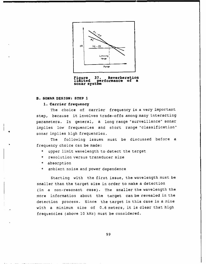
d8 \L - I

Limitingrange

Range

Figure 37. Reverberationlimited performance of asonar system

B. SONAR DESIGN: STEP 1

1. Carrier frequency

The choice of carrier frequency is a very important

step, because it involves trade-offs among many interacting

parameters. In general, a long range "surveillance" sonar

implies low frequencies and short range "classification"

sonar implies high frequencies.

The following issues must be discussed before a

frequency choice can be made:

* upper limit wavelength to detect the target

* resolution versus transducer size

* absorption

* ambient noise and power dependence

Starting with the first issue, the wavelength must be

smaller than the target size in order to make a detection

(in a non-resonant case). The smaller the wavelength the

more information about the target can be revealed in the

detection process. Since the target in this case is a mine

with a minimum size of 0.6 meters, it is clear that high

frequencies (above 10 kHz) must be considered.

99

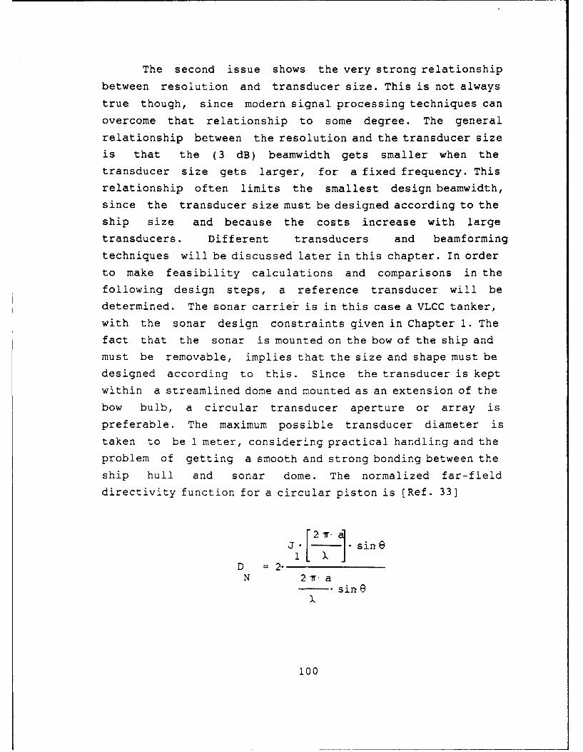
The second issue shows the very strong relationship

between resolution and transducer size. This is not always

true though, since modern signal processing techniques can

overcome that relationship to some degree. The general

relationship between the resolution and the transducer size

is that the (3 dB) beamwidth gets smaller when the

transducer size gets larger, for a fixed frequency. This

relationship often limits the smallest design beamwidth,

since the transducer size must be designed according to the

ship size and because the costs increase with large

transducers. Different transducers and beamforming

techniques will be discussed later in this chapter. In order

to make feasibility calculations and comparisons in the

following design steps, a reference transducer will be

determined. The sonar carrier is in this case a VLCC tanker,

with the sonar design constraints given in Chapter 2. The

fact that the sonar is mounted on the bow of the ship and

must be removable, implies that the size and shape must be

designed according to this. Since the transducer is kept

within a streamlined dome and mounted as an extension of the

bow bulb, a circular transducer aperture or array is

preferable. The maximum possible transducer diameter is

taken to be 1 meter, considering practical handling and the

problem of getting a smooth and strong bonding between the

ship hull and sonar dome. The normalized far-field

directivity function for a circular piston is [Ref. 33]

1 [. 1 sineD =2-N 2ira

sine

100

where a = radius

e = polar angle in spherical coordinatesJl()= first order Bessel function of the first

kind

From this an approximate expression for the 3 dBbeamwidth can be derived [Ref. 34):

65BW (in degrees)2

-

d

where lambda is the wavelength and d is the transducerdiameter. A simple calculation indicates that to achieve abeamwidth of less than one degree (conical beam) the carrier

frequency must exceed 100 kHz. Since the target isrelatively small in size, it will be necessary to use very

narrow beams, probably fractions of a degree. This impliesthat carrier frequencies of 100 kHz and above must be used.

The third issue counteracts the usage of highfrequencies due to the increasing energy absorption athigher frequencies. The absorption depends mainly on thesalinity in the water, which gives an advantage of usinghigh frequencies in the Baltic vice the Atlantic Ocean (seeChapter 6). However, even in the Baltic the absorption willbe very significant, when using frequencies above 100 kHz,

as can be seen in Table 18.

The fourth issue indicates that the ambient noise andtransmitting power must be considered before determining thefrequency. As can be seen in Appendix 0, the decliningambient noise with frequency has a break point around 100kHz and will then increase with frequency. This ambient

101

TABLE 18. ABSORPTION RATES

frea (kHz) absorption (dB/km)100 10200 20

300 30500 100

noise is due to molecular movement in the water. In order to

keep the NSL down, frequencies in the lower region, around

100 kHz are preferable. The power limitation works the

opposite way. Higher frequencies allow higher power levels

to be transmitted into the ocean. This is due to cavitation

effects on the sonar surface and will be further treated

later in this chapter.

A target's resonance region for spheres is determined

by the factor ka, where k = 2 ir / ) and a is the targetradius. The resonance region is usually in the ka interval

2-30. Hence, if the speed of sound is 1500 m/s the target's

resonance frequency can be found in the interval [Ref. 35]:

1500 22500f = - , (Hz)

ir.a .a

In this case a = 0.6, so the resonance frequencies

must be somewhere between 796 Hz and 12 kHz. A transmitted

signal with a frequency in this interval could trigger the

target's resonances. As mentioned in Chapter 2, this can

enhance the target strength (TS) but it can also lower it,

if the target has high internal losses or if the reradiated

sound is radiated in directions other than the specular

direction. [Ref. 9] In order to utilize the resonance

102

phenomena, experiments must be performed to first determinethe resonance frequencies for the particular target and thenmeasure how the target strength varies. Since in this casethe target can have many different shapes and these shapesare practically always unknown, the technique has manydisadvantages and can probably not be utilized. Furtherresearch and experiments must be performed to investigate

this.

To determine an optimum frequency is not an obviousthing to do. Especially since the assumption is that ofreverberation limited performance, where the frequencydependent absorption coefficient is essentially the same forthe echo and for the reverberation background [Ref. 6].

There must be a trade-off decision with the parameters aboveas input values. One conclusion is that with the detectionrange requirement stipulated in the introduction to this

chapter, the frequency range must be within 100 - 500 kHz,mainly in order to balance transducer size and absorption.

In order to make comparisons and facilitate the finaldecision, it is advisable to carry along both limiting

frequencies, 100 and 500 kHz, in the design.

2. Transmission loss (TL)

To detect a target, transmitted energy (sound wave)from the transducer must find a path to the target and back

to the transducer. Since the speed of sound, with which theenergy is propagating, is a function of salinity, pressureand the temperature of the propagating medium, differentspeeds of sound will occur at different locations. The speedof sound differences have the effect of refracting theenergy in a direction dependent on the gradient. In this

case the most significant speed of sound differences occuras a function of water depth. If the required detection

range had been greater than 1,000 meters, the speed of sounddifferences in azimuthal distance had also been important.

103

The energy propagation or sound field can be described withrays which obey "Snell's laws" of refraction, and a raytracing diagram can be produced for a specific speed ofsound profile. There are a number of limitations in the raytracing concept, since both boundaries (surface and bottom)are assumed to be flat and rigid. Further, no estimation ofenergy scattered into shadow zones is indicated. A raytracing program [Ref. 36] has been used in Appendix M, toshow the propagating sound field for monthly average speedof sound profiles and different source depths. Afterdiscussing the sonar concept with different references [Ref.30, 36] the conclusion is that there must be a direct pathbetween the transducer and the target, in order to achievereliable detection criteria. Ray reflections from theboundaries can cause multipath effects and disturb thedirect ray echo return. This will be further investigatedlater. When examining the ray diagrams in Appendix M, directray paths can be found for all months except June, July andOctober, with the source at 10 meters depth. The summer is adifficult season, due to the very strong negative gradient,which causes the rays to strongly refract toward the bottomand create a sharp shadow zone. The shadow zone is notcompletely dark, however. Some sound energy exists in thezone and measurements have been done at 24 kHz that gave TLvalues between 20 to 70 dB/Kyd close to the boundary. [Ref.9] Sound waves propagating in the ocean normally getdelayed, distorted and weakened during their transition.This is due to the nature of boundary layers, absorption andthe geometrical spreading of the sound field. Thesephenomena can be taken together in a transmission loss (TL)factor, which is defined as the weakening of sound between apoint 1 meter from the source and another point at adistance in the sea. [Ref. 9]

104

Since at this stage only the direct sound path isconsidered, and because of the short range requirements,

only absorption and geometrical spreading will influence our

TL factor. In a sound channel the sound is first spreadspherically out to a transition range, which can beestimated by the following formula, valid for a mixed layerwith a positive speed of sound gradient near the sea surface

[Ref. 7]:

2D

r =105t D - Z

where Z = source depth

D = depth of mixed layer

Beyond this range the spreading will becomecylindrical and if the two boundary layers are accounted

for, something in between spherical and cylindrical will

occur. The TL formulas for the two spreading forms are [Ref.

32]:

Spherical spreading: TL = 20 log r

Cylindrical spreading: TL = 10 log rUsing the formula above and comparing with the speed

of sound profiles in Appendix P, the transition range willexceed 1,000 meters for all months, and since 700 meters is

less than that, only spherical spreading needs to be used.Adding the absorption loss to the spherical spreading gives

the following expression [Ref. 32]:

TL = 20 log r + ar (Equation 1)where a = absorption

r = range

The absorption at different frequencies is found inTable 18 above and the TL for the two carrier frequencies

and range limits are shown in Table 19.

105

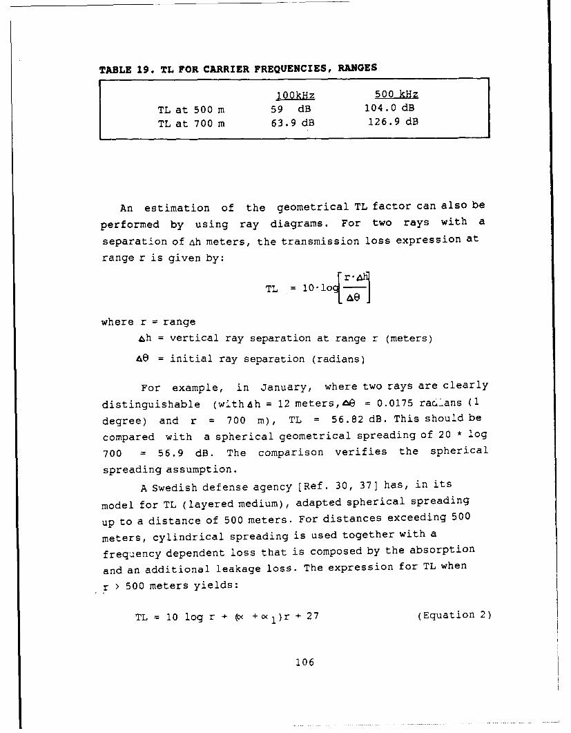
TABLE 19. TL FOR CARRIER FREQUENCIES, RANGES

100kHz 500 kHz

TL at 500 m 59 dB 104.0 dB

TL at 700 m 63.9 dB 126.9 dB

An estimation of the geometrical TL factor can also be

performed by using ray diagrams. For two rays with a

separation of ah meters, the transmission loss expression at

range r is given by:

TL = lol --[±

where r range

h= vertical ray separation at range r (meters)

4e = initial ray separation (radians)

For example, in January, where two rays are clearly

distinguishable (w'th4h = 12 meters,4 = 0.0175 raclans (1

degree) and r = 700 m), TL = 56.82 dB. This should be

compared with a spherical geometrical spreading of 20 * log

700 = 56.9 dB. The comparison verifies the spherical

spreading assumption.

A Swedish defense agency [Ref. 30, 37] has, in its

model for TL (layered medium), adapted spherical spreading

up to a distance of 500 meters. For distances exceeding 500

meters, cylindrical spreading is used together with a

frequency dependent loss that is composed by the absorption

and an additional leakage lose. The expression for TL when

r > 500 meters yields:

TL = 10 log r + (oK +o<1)r + 27 (Equation 2)

106

where 27 dB is the TL up to 500 m

= absorption coefficient

oi= leakage coefficient

The leakage coefficient decreases with frequency andis linear in a logarithmic scale. The expression for the

leakage coefficient (32 Hz - 8 kHz) yields:

i = 1.88 - 0.42 log f

With the assumption that this relationship holds even for

higher frequencies (100 and 500 kHz), the leakagecoefficient will become zero and Equation 2 will become the

same as the original TL Equation 1 above.

The following conclusions can be made based on the

results above:* The source depth must be at approximately 10 meters,

in order to get most direct paths to the target.

The spherical spreading with absorption (Equation i)expression can Ee used as the TL term in the activesonar equation.

* "Safe" ship operation will not be possible the entireyear.

3. Resolution, waveform and target detection

The resolution of a sonar system can be defined byeither its measuring precision or its detection capability

and depends on:* the pulse length

* the beamwidth

* the target strength (TS)

* the angle of incident upon the target

* the display and recording technique

The pulse length choice has three importantimplications. First, it determines the range resolution ofthe system. Second, it determines how much of the total

target strength can be utilized. Third, it determines the

reverberation element in length. The pure range resolution

107

is of minor importance in this case, since it is very

unlikely that two mines are deployed very closely together.

Of more importance is to minimize the reverberation element

as much as possible. Further, in order to get full usage of

the target strength, the pulse width must fully ensonify the

target [Ref. 10). For this latter reason the following

expression for pulse width must be used:

Ar*2T = -

c

where Ar = resolution in meters

c = speed of sound

A 4r of 0.6 meters and c of 1500 m/s gives a pulsewidth of 0.8 ms. The expression for range resolution is

Pulsewidth * C2

which gives a range resolution of

0.8 ms * 1500 = 0.6 meters

2

This means that if two mines are deployed with less than 0.6meters between them (which is very unlikely), the echo

return will contain both targets and they cannot bedistinguished. Hence, the combination of utilizing the full

target strength, together with getting minimum reverberation

element in length, yields a pulse duration of 0.8 ms.

The return pulse will be stretched out in time by

2*L/c seconds, where L is the target range dimension [Ref.

7]. Using L = 0.3 (since spherical or cylindrical mine

108

shape) the returning echo will be 1.2 ms long. The fact that

the ship is moving toward the mine, with a speed of 16 knots(8 m/s), counteracts this pulse stretching. Using Ziomek[Ref. 33:p. 200], a time-compression'stretch factor can becalculated using the expression (for this case only):

(1 - b)S =

(1 - c)

where b = - 0.0053 and c = 0.0053 s is then equal to 1.011.Comparing this (reciprocal value) with the pulse length 0.8

ms, gives a pulse compression effect of 0.01 ms. Theconclusion is that the time compression, due to the ship

speed, has only a minor impact on the returning pulse. Thereturning pulse will consequently be 1.2 ms - 0.01 ms = 1.19

ms long. This determines the receiver bandwidth to be at

least 1/T = 840 Hz.

The angle of incidence upon the target has very littleeffect in this case, because the shape of the mine isspherical or cylindrical. The angle of incidence would be of

more importance, though, if the mine had been deployed on

the bottom.

The last issue above, the display and recordingdevice, will not be covered in this thesis. It is assumedthat these devices are chosen to present the resolution

necessary to fulfill the sonar objective.

The detection threshold (DT) of a sonar system isdefined as the input minimum signal-to-noise power ratio,within the bandwidth of the system, that; after all

processing (mental analysis) of the received stimulus

(signal plus noise) is completed; will guarantee a givenprobability of detection (P(D)) for a specified probability

of false alarm (P(FA)). [Ref. 71 The detection threshold

expression depends on the detection index, that is the value

109

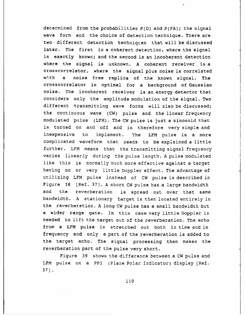
determined from the probabilities P(D) and P(FA); the signal

wave form and the choice of detection technique. There are

two different detection techniques that will be discussed

later. The first is a coherent detection, where the signal

is exactly known; and the second is an incoherent detectionwhere the signal is unknown. A coherent receiver is acrosscorrelator, where the signal plus noise is correlatedwith a noise free replica of the known signal. The

crosscorrelator is optimal for a background of Gaussiannoise. The incoherent receiver is an energy detector that

considers only the amplitude modulation of the signal. Two

different transmitting wave forms will also be discussed;

the continuous wave (CW) pulse and the linear frequency

modulated pulse (LFM). The CW pulse is just a sinosoid that

is turned on and off and is therefore very simple and

inexpensive to implement. The LFM pulse is a morecomplicated waveform that needs to be explained a littlefurther. LFM means that the transmitting signal frequency

varies linearly during the pulse length. A pulse modulated

like this is normally much more effective against a targethaving no or very little Doppler effect. The advantage of

utilizing LFM pulse instead of CW pulse is described in

Figure 38 [Ref. 37]. A short CW pulse has a large bandwidthand the reverberation is spread out over that samebandwidth. A stationary target is then located entirely in

the reverberation. A long CW pulse has a small bandwidth but

a wider range gate. In this case very little Doppler isneeded to lift the target out of the reverberation. The echo

from a LFM pulse is stretched out both in time and in

frequency and only a part of the reverberation is added to

the target echo. The signal processing then makes the

reverberation part of the pulse very short.

Figure 39 shows the difference between a CW pulse and

LFM pulse on a PPI (Plane Polar Indicator) display [Ref.

37].

110

f f

re{drb rerb dist

long pulse

short pulse

dist

FM pulse

Figure 38. The LFM waveform advantage

, TARGET .TRE

CW LINEAR FM

Figure 39. Difference between an LFM pulse and a CW pulse ona PPI.

A variation of the pulsed LFM modulation is the

Continuous Transmission Frequency Modulation (CTFM). The

frequency modulated signal is continuously transmitted and

the different frequencies of the outgoing and incoming

signal are determined. This freque ° cy difference is a

111

measure of the target distance. CTFM sonar gives very good

audio information of the echo structure of the target, which

can be used for detection and classification [Ref. 37]. The

major disadvantage with a CTFM sonar is that two apertures

or arrays must be used and there must be good isolation

between i-ne two. Due to the practical disadvantages with

such a system and the increasing costs, this modulation type

will be of minor interest.

The DT expressions for different detection techniques

and wave forms will now be discussed. DT expressions from

three different references will be covered, since there are

differences between them. The pulse duration will be the

same for both pulse forms in the calculations in order to

obtain a comparison. The design criteria for swept bandwidth

and pulse lengch is found in Ziomek [Ref. 33] and yields:

4-7

IbI T2

where lb I = phase deviation constant (rad/sec2 )T = pulse lengthWith a return pulse length of 0.8 ms and the

inequality set to one, the swept bandwidth must be 5 kHz. By

setting the inequality to 1, the range resolution will

decrease to 0.3 meters, when not considering the pulse

stretching discussed above. Since the carrier frequencies

are up in the 100/500 kHz range, a swept bandwidth of 5 kHz

still makes the signal to be "narrowband." In all tne

calculations below, a return signal pulse length of 1.2 ms

will be used. For detection index and the "delta"

calculations, the curves in Appendix P will be used.

112

a. Incoherent detection

Urick assumes in his book [Ref. 9) that the

reverberation is "noise like" and describes a "rule of

thumb" expression for the DT as follows:

DT = 5- lo[2 -10 logW' +4 (1

where d = detectivity index (from ROC curves in Appendix P)

w = receiver bandwidth

w' = reverberation bandwidth

T = pulse length

= compensation factor for small bandwidth products

(Appendix P).

Urick refers to a paper by Kroenert [Ref. 38] for

information about different DT expressions. Kroenert's

expressions are based on Urick's assumptions and yield:

DT(CW) = 10 * log (T *f ) + 10 *log T (2)

DT(LFM) = 5 * log (d * T/w') + - 10 * log T (3)

The third reference is from Burdick's book [Ref. 7]

and he assumes that the target signal and the reverberation

have the same spectral shape and no processing advantages,

with different filter techniques, can be gained. The DT

expression, derived in this book, is directly related to

this application, with a stationary target and reverberation

limited performance. The DT is then a function depending

only on the detection index.

DT = 5 * log d (4)

where d is obtained from the ROC curves for a unity time

bandwidth product (d = 75).

The numerical values for the above expressions are:

113

Using Equation 1 with:

d=detectivity index (from ROC curves Appendix P)=1

w = receiver bandwidth = 833 Hzw'=reverberation bandwidth=5 kHz with LFM, 833 with CW

T = pulse length = 1.2 ms

A= (from Appendix P) 1.5 for LFM and 3 for CW yields:

DT(CW-pulse) = 8.3 dB

DT(LFM-pulse) = - 0.6 dB

Using Equations 2 and 3 with the same values as above

yields:

DT(CW-pulse) = 8.2 dB

DT(LFM-pulse) = 3.3 dB

Using Equation 4 with d = 75 yields:

DT(CW-pulse) = 9 dB

b. Coherent detection:

Only Kroenert's paper gives expressions for DT with acoherent receiver.

DT(CW-pulse) = 10 * log (d * T/2) - 10 * log T

DT(LFM-pulse) = 10 * log (d/ (2 *w')) -10 * log T

Using the same values as above yields:

DT(CW-pulse) = 7.4 dB

DT(LFM-pulse) = -0.4 dB

In conclusion, since a coherent detection technique isoptimized for Gaussian noise (which is not the case here), anincoherent detection technique must be the most appropriate inthis design. Later in the chapter it will also be concluded thatthe impact of multipath interference supports a choice of an

114

incoherent receiver technique, especially in an active sonar

application. Using an incoherent detection technique gives anumber of DT choices as shown above. An LFM waveform givesthe lowest DT in all cases, as expected. The problem withusing LFM is that it is a much more sophisticated technique,which implies higher costs both for purchase of the sonarand for maintenance. These are not desirable factors whenconsidering the main objective of the design. This implies,

that if the detection goal can be fulfilled with a CW pulse,this must be a preferable waveform. Therefore, a CW pulse is

chosen to be the main alternative, and a "worst case" DT of+9 dB is adopted for the further design.

The returning carrier frequency will be shifted upin frequency due to the ship's speed (Doppler effect). The

returning pulse length will also be stretched from 0.8 ms to1.19 ms. This makes the necessary receiver bandpass filterdecrease from 1250 Hz to 840 Hz. The bandpass filter must becentered due to the Doppler shifted carrier frequency, that

is at 101.1 kHz for a 100 kHz transmitted frequency and at505.3 kHz for a 500 kHz transmitted frequency. In order tomake the receiver susceptible to changeable ship speeds, aparallel filter solution can be considered. This will

increase the cost, though.

C. SONAR CONCEPT

The main objective of the sonar is to detect a target,

i.e., a mine. A refinement of this objective is to include aclassification of the detected target. This would

discriminate against "false targets" and avoid unnecessary

ship maneuvers. This part of the chapter will investigatewhether it is possible to design such a sonar for this

application or not. It will be shown that only aconventional "classification" sonar design is possible to

pursue.

115

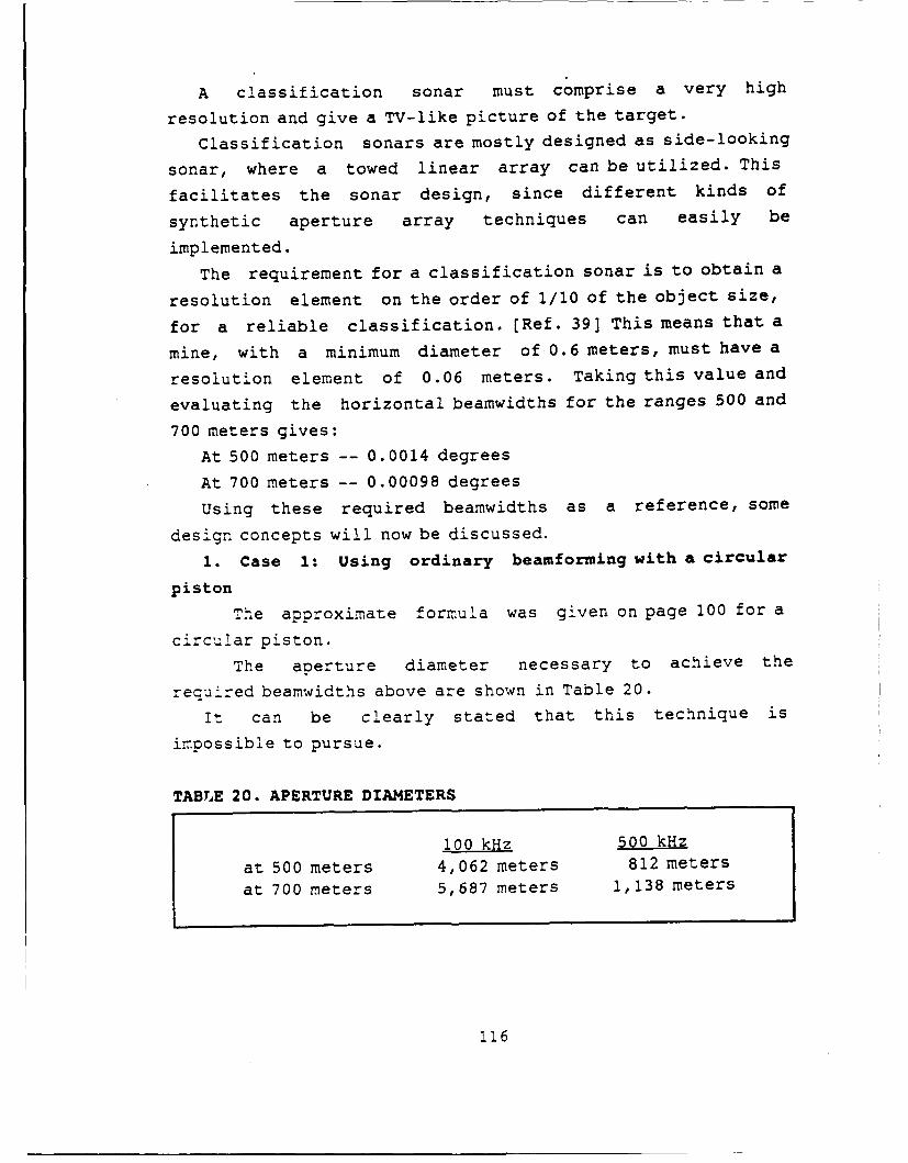
A classification sonar must comprise a very high

resolution and give a TV-like picture of the target.

Classification sonars are mostly designed as side-looking

sonar, where a towed linear array can be utilized. This

facilitates the sonar design, since different kinds of

synthetic aperture array techniques can easily be

implemented.

The requirement for a classification sonar is to obtain a

resolution element on the order of 1/10 of the object size,

for a reliable classification. [Ref. 39] This means that a

mine, with a minimum diameter of 0.6 meters, must have a

resolution element of 0.06 meters. Taking this value and

evaluating the horizontal beamwidths for the ranges 500 and

700 meters gives:

At 500 meters -- 0.0014 degrees

At 700 meters -- 0.00098 degrees

Using these required beamwidths as a reference, some

design concepts will now be discussed.

1. Case 1: Using ordinary beamforming with a circular

piston

The approximate formula was given on page 100 for a

circular piston.

The aperture diameter necessary to achieve the

required beamwidths above are shown in Table 20.

It can be clearly stated that this technique is

impossible to pursue.

TABLE 20. APERTURE DIAMETERS

100 kHz 500 kHz

at 500 meters 4,062 meters 812 meters

at 700 meters 5,687 meters 1,138 meters

116

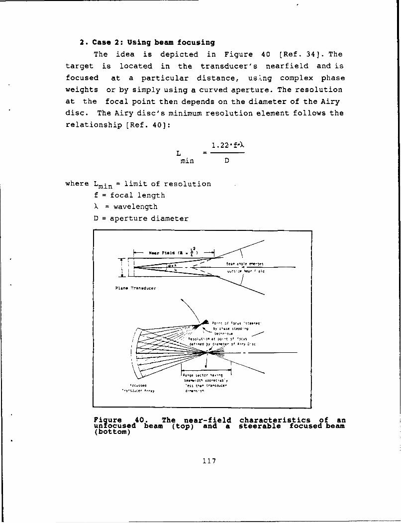
2. Case 2: Using beam focusing

The idea is depicted in Figure 40 [Ref. 34]. The

target is located in the transducer's nearfield and is

focused at a particular distance, using complex phaseweights or by simply using a curved aperture. The resolution

at the focal point then depends on the diameter of the Airy

disc. The Airy disc's minimum resolution element follows the

relationship [Ref. 40]:

1. 2 2. fLmin D

where Lmin = limit of resolution

f = focal length

)= wavelength

D = aperture diameter

Plane Transducer

9& ~ n ' O, f locus 'steereo'

_b ;ase steop'ng

'4esolutl on at dollt 2f

loc's

*tfined py dameter of Airy Disc

Ranqe sector "a,,nqbeamw1dth aborec1ably

rocussed 'ess tan transduCer

',lae Array meSl

Fiqure 40. The near-field characteristics of anun ocused beam (top) and a steerable focused beam(bottom)

117

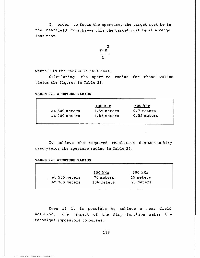
In order to focus the aperture, the target must be inthe nearfield. To achieve this the target must be at a range

less than

2T R

where R is the radius in this case.

Calculating the aperture radius for these values

yields the figures in Table 21.

TABLE 21. APERTURE RADIUS

100 kHz 500 kHzat 500 meters 1.55 meters 0.7 metersat 700 meters 1.83 meters 0.82 meters

To achieve the required resolution due to the Airy

disc yields the aperture radius in Table 22.

TABLE 22. APERTURE RADIUS

100 kHz 500 kHzat 500 meters 76 meters 15 metersat 700 meters 106 meters 21 meters

Even if it is possible to achieve a near field

solution, the impact of the Airy function makes the

technique impossible to pursue.

118

To achieve high resolution, in this application, isnot an obvious and easy task. Even with different kinds of

traditional array shading techniques, beamwidths like 0.0014

degrees are impossible to get. Maybe new signal processing

techniques, like the frequency domain adaptive beamformingtechnique can narrow down the beamwidth to what is required.

The conclusion is that the design must be restricted to a

traditional classification sonar, and the necessary

beamwidth will be decided using the reverberation limited

active sonar equation.

D. MULTIPATH PROPAGATION STUDY

Multipath propagation originates with a single sonar

induced by pulses whose reflected paths arrive at the

receiver at different times due to sound bending in thewater and reflections from the sea surface and the sea

bottom. Multipath propagation occurs primarily with ducted

propagation and in shallow water. The major multipath

propagation effects are:* signal fluctuations in amplitude and phase

* signal distortion

* signal decorrelation in amplitude and phase

* frequency broadening

The signal fluctuation can cause fading effects, which

means that the target detectability decreases. Signal

distortion degrades coherent detection. Decorrelation

adversely effects the beam forming properties of

multi-element arrays. Finally, frequency broadening implies

that a wider receiver bandwidth must be used, which

increases the noise and reverberation in the detection

process. Therefore, multipath propagation is a very unwanted

phenomena. It will be shown that multipath is not a major

problem for this design due to the short wavelength and

rough boundaries. (Ref. 9, 41]

119

There are essentially three propagation paths, excludingthe direct path, that can cause multipath effects in this

application.* the surface reflecting path

* the bottom reflecting path

* paths due to the thermal microstructure in the water

Figure 41 shows the theoretical multipaths to the target,based on the geometry, that can occur in this case.

Transducer 700m Target

0 BA0 Surface

147 Bottom

a. surface reflecting path

b. direct path

c. path due to microstructure in the water

d. bottom reflecting path

Figure 41. Propagation paths between transducer and target

The surface reflecting path is particularly important toconsider when the source and target lie at a shallow depth.

Because the path difference between the direct and reflectedwave path is small, the target is in the image interference

field where, depending on path differences, both waves'

intensities constructively or destructively interfere with

each other. This phenomena is very significant when thesurface is smooth and the incident grazing angle of the

120

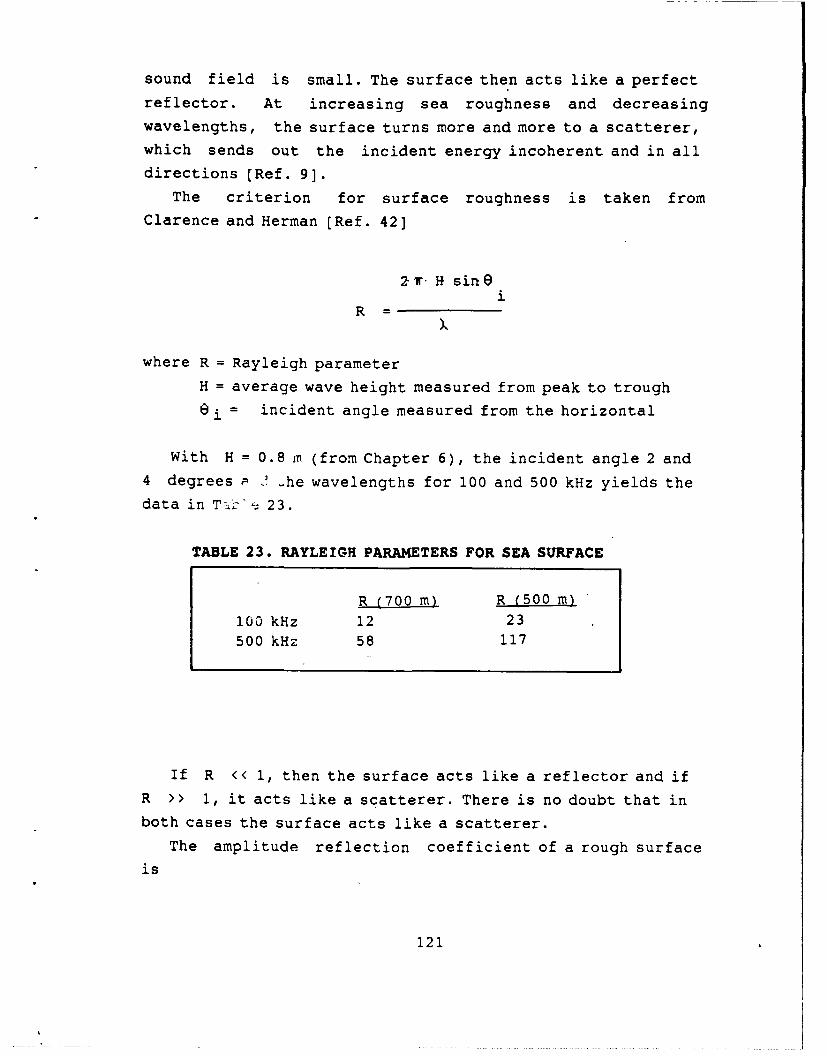
sound field is small. The surface then acts like a perfect

reflector. At increasing sea roughness and decreasingwavelengths, the surface turns more and more to a scatterer,which sends out the incident energy incoherent and in all

directions [Ref. 9].

The criterion for surface roughness is taken from

Clarence and Herman [Ref. 42]

2T" H sinei

R=

where R = Rayleigh parameter

H = average wave height measured from peak to trough

ei = incident angle measured from the horizontal

With H = 0. 8 m (from Chapter 6), the incident angle 2 and4 degrees -. .he wavelengths for 100 and 500 kHz yields the

data in Tz,17 23.

TABLE 23. RAYLEIGH PARAMETERS FOR SEA SURFACE

R (700 m) R (500 m)100 kHz 12 23

500 kHz 58 117

If R << 1, then the surface acts like a reflector and ifR >> 1, it acts like a scatterer. There is no doubt that inboth cases the surface acts like a scatterer.

The amplitude reflection coefficient of a rough surface

is

121

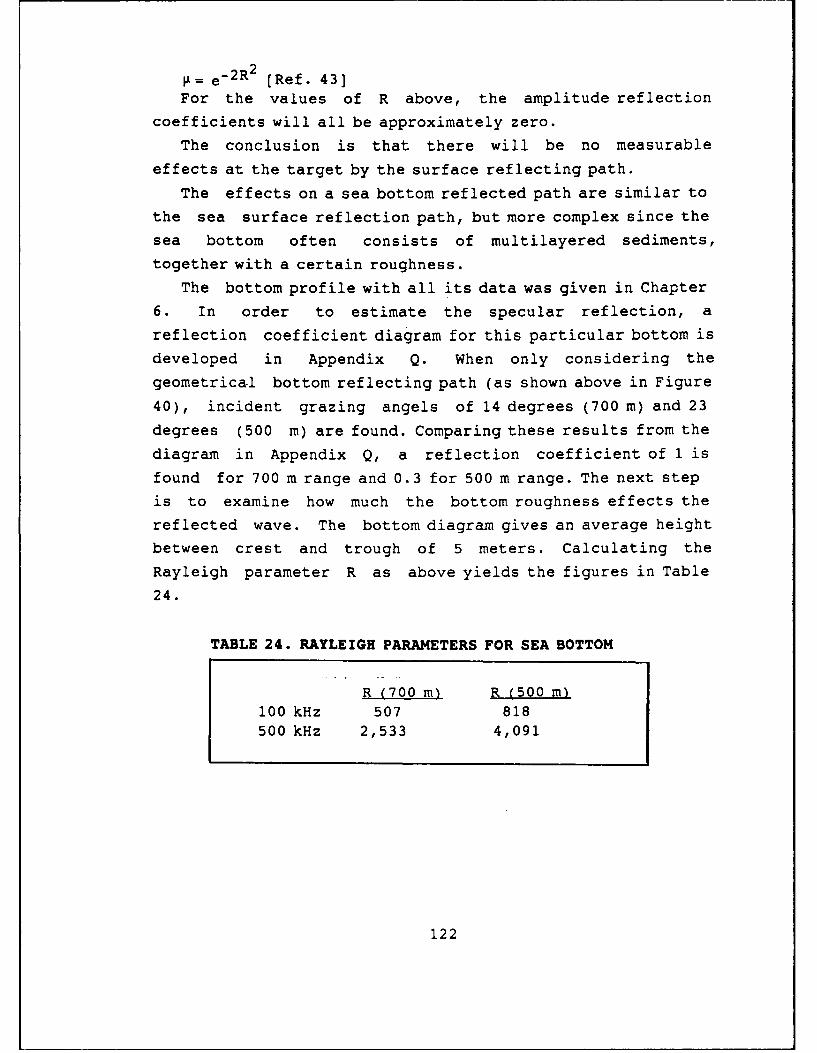
e- 2R 2 [Ref. 43]For the values of R above, the amplitude reflection

coefficients will all be approximately zero.

The conclusion is that there will be no measurable

effects at the target by the surface reflecting path.

The effects on a sea bottom reflected path are similar to

the sea surface reflection path, but more complex since the

sea bottom often consists of multilayered sediments,

together with a certain roughness.

The bottom profile with all its data was given in Chapter

6. In order to estimate the specular reflection, a

reflection coefficient diagram for this particular bottom is

developed in Appendix Q. When only considering the

geometrical bottom reflecting path (as shown above in Figure

40), incident grazing angels of 14 degrees (700 m) and 23

degrees (500 m) are found. Comparing these results from the

diagram in Appendix Q, a reflection coefficient of 1 is

found for 700 m range and 0.3 for 500 m range. The next step

is to examine how much the bottom roughness effects the

reflected wave. The bottom diagram gives an average height

between crest and trough of 5 meters. Calculating the

Rayleigh parameter R as above yields the figures in Table

24.

TABLE 24. RAYLEIGH PARAMETERS FOR SEA BOTTOM

R (700 m) R (500 m)100 kHz 507 818500 kHz 2,533 4,091

122

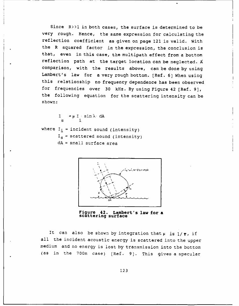
Since R>>1 in both cases, the surface is determined to bevery rough. Hence, the same expression for calculating thereflection coefficient as given on page 121 is valid. Withthe R squared factor in the expression, the conclusion isthat, even in this case, the multipath effect from a bottomreflection path at the target location can be neglected. Acomparison, with the results above, can be done by usingLambert's law for a very rough bottom. [Ref. 6] When usingthis relationship no frequency dependence has been observedfor frequencies over 30 kHz. By using Figure 42 (Ref. 9],the following equation for the scattering intensity can beshown:

I = I sin) dAs i

where Ii = incident sound (intensity)is = scattered sound (intensity)

dA = small surface area

\

I, S A/

\,Sn8s 0C

\ -

Figure 42. Lambert's law for ascattering surface

It can also be shown by integration that t is j/1 , ifall the incident acoustic energy is scattered into the uppermedium and no energy is lost by transmission into the bottom(as in the 700m case) [Ref. 9]. This gives a specular

123

surface reflection coefficient of 0.019, taking bothincident and reflecting angle to be 14 degrees. This resultsupports the conclusion above that the bottom reflecting

path is negligible.

The third multipath cause to consider is due to the lackof homogeneous sea temperatures that constantly change thi

index of refraction. These temperature changes occur likecells in the direct path between the source and target. Eachcell bends the sound ray differently, depending on thelaunch angle. As a result, when they converge at the target,multipath effects occur. Different equations estimating thecell sizes and sound velocity deviation and their impact onthe transmitted pressure pulse are developed by Urick [Ref.

9, 41]. There are no data available in order to do

estimations in this case.

In conclusion, the multipath results above support theassumption that only the use of a direct sound path betweenthe source and the target is reliable in making a target

detection. Even if the interacting sound at the targethappens to be small, it is recommended that the verticalbeam pattern be minimized as much as possible to reduce boththe multipath and the back scattering (reverberation)effects. When studying the ray diagrams in Appendix 0, thedepression angle must be on the order of 10 degrees toensure the propagation of all direct rays. If no direct rayscan be found, the chances of detecting the target are very

small, despite some scattering into the shadow zones.

E. SONAR DESIGN: STEP 2

1. Back-scattering strength study

In active sonar systems, the returning echo signalcomprises both reflections from the target and reflections

from the sea surface, the sea bottom and from the watervolume. The undesired echo contribution is called

124

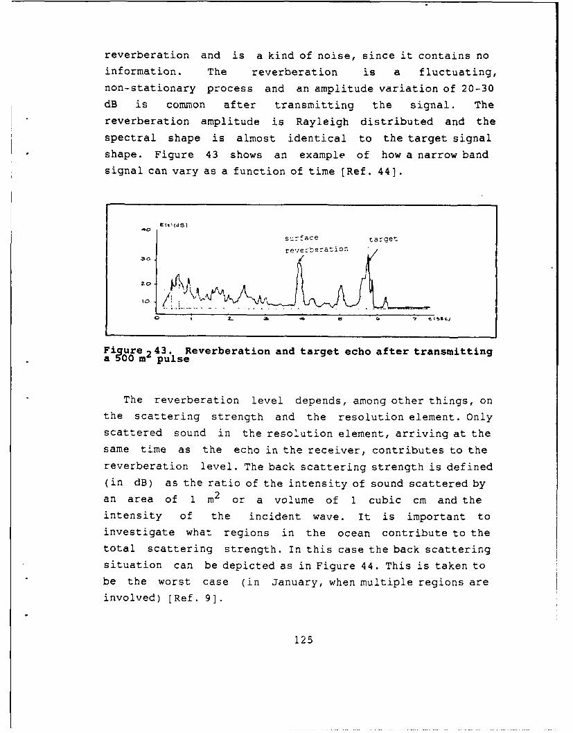
reverberation and is a kind of noise, since it contains no

information. The reverberation is a fluctuating,

non-stationary process and an amplitude variation of 20-30

dB is common after transmitting the signal. The

reverberation amplitude is Rayleigh distributed and the

spectral shape is almost identical to the target signal

shape. Figure 43 shows an example of how a narrow bandsignal can vary as a function of time [Ref. 44).

C (t I(d 5)

surface target

reverberation

Figure 243. Reverberation and target echo after transmittinga 500 m pulse

The reverberation level depends, among other things, on

the scattering strength and the resolution element. Only

scattered sound in the resolution element, arriving at the

same time as the echo in the receiver, contributes to the

reverberation level. The back scattering strength is defined(in dB) as the ratio of the intensity of sound scattered by

an area of 1 m2 or a volume of 1 cubic cm and the

intensity of the incident wave. It is important to

investigate what regions in the ocean contribute to the

total scattering strength. In this case the back scatteringsituation can be depicted as in Figure 44. This is taken to

be the worst case (in January, when multiple regions are

involved) [Ref. 9].

125

The following back scattering regions will be further

investigated:* Surface scattering: surface reflection and bottom

reflection* Surface scattering by a layer of volume scatterers:

air bubbles down to 3 meters depth and fish densitydown to 40 meters depth

700 m

0 m -20 m Surface

10 Target

-777 Bottom

Figure 44. The back scattering regions

The surface scattering for both the sea surface andthe sea bottom, has already been investigated in thischapter. The fact that the surfaces are very rough compared

to the wavelengths, makes them "scatterers" and the sound is

scattered out in all directions incoherently. The seasurface reflection coefficient gives unmeasurably smallvalues when using the Rayleigh scattering model above. The

conclusion is that, when using this model, the backscattering contribution is negligible. The Rayleigh model

gives the same small reflection coefficient for the seabottom which also implies negligible back scattering there.

126

Using the Lambert's Law model instead gives the following

equation:

2SB = 10 log .& + 10 log sine

where I = 1/iT [Ref. 9]

For a grazing angle of 10 degrees, the scattering

coefficient becomes -20 dB.

Urick [Ref. 9] gives values for bottom scattering

strengths vice grazing angles that are based on many

measurements and frequencies up to 100 kHz (Figure 45), but

does not indicate bottom roughness.

S-20

-30

-40 1 I I I I I

2 5 0 20 50 90

Grazin anle. deg

Figure 45. Bottom backscattering strengthas a function of grazing angle

A 10 degree grazing angle gives SB = - 38 dB for

clay.

The values above are quite far from each other. Since

the speed of sound gradients, during most of the year, are

negative, the sound waves are most often bending down toward

127

the bottom. Hence, the bottom scattering region is moreimportant to consider than the sea surface. Therefore, aworst case value of -20 dB will be assigned as the total

back scattering from both surfaces."Surface scattering with layer of volume scatterers"

models can be used when there are scatterers in layers, such

as bubbles and fish. However, instead of calculating avolume scattering situation, the finite layer concept maktes

it possible to use a surface scattering model. The surfacescattering strength Ss is then:

Ss = Sv + 10 * log H [Ref. 9)

where H = layer depth

Air bubbles are most frequently located in a layernear the surface, and their sizes and numbers depends on theagitation of the sea surface (wind and waves) and the water(fresh water, ocean water, coastal water, etc.). No measuredvalues of bubble sizes and densities have been available forthe Baltic, so an estimation must be made. Clarence andHerman [Ref. 42:p. 173] show a figure that summarizes bubble

content in water determined by experiments.

For coastal waters there is an average of 103

bubbles per cubic meters at 3.3 meters. Their sizes reachfrom 1 m to 40 m, so an average size of 20 m will be usedfor the calculations. The bubbles' back scattering can be

computed as follows [Ref. 9]:

I siSv = lot log~ - (1)

where a = scattering cross section

128

n = bubbles /yd3 [Ref. 9]

To find the scattering cross section, the following

equation applies:2

4w. a

s 2

f (2)

r 2

where fr = bubble resonant frequency

S= damping constant [Ref.91

Further, the bubbles' resonance frequency must be

calculated according to the following equation:

326fr = 1 + 0.03 d

a (3)

where d = depth in feet [Ref.9]To compute the scattering cross section in Equation 2,

the damping constant of air bubbles in water must be

determined. This damping constant is a measure of the

dissipation process in the bubbles and is the reciprocal of

the bubbles' Q (Quality factor). Figure 46 gives the

theoretical damping of resonant bubbles in water [Ref. 9].

Using Equation 3 with the values for bubble radius and

the depth indicated above, the bubble resonant frequency is

186 kHz. Then calculating the scattering cross section for

both frequencies (100 and 500 kHz) together with a damping

constant of 0.1 gives:

129

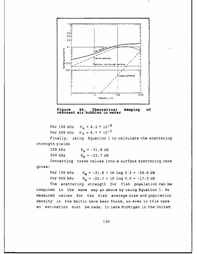
o.III- I'04-03-02

0 /

C0

0 ~odtiorl (scctterinq) daoiNon

001 / / -

/ j

1C 100 1.000Fr~uenCy, KHZ

Figure 46. Theoretical damping ofresonant air bubbles in water

For 100 k~z CS= 8.3 * 10-6

For 500 kHz os = 6.7 * 10-5

Finally, using Equation 1 to calculate the scattering

strength yields

100 kHz SS = -31. 8 dB

500 kHz S5 = -22.7 dBConverting these values into a surface scattering case

gives:

For 100 kHz Sa = -31.8 + 10 log 3.3 = -26.6 dBFor 500 kHz Sa = -22.7 + 10 log 3.3 = -17.5 dB

The scattering strength for fish population can becomputed in the same way as above by using Equation 1. No

measured values for the fish average size and population

density in the Baltic have been found, so even in this case

an estimation must be made. In Lake Michigan in the United

130

States, fish density samples have been taken for variousdepths and locations. An average fish density of 5.7 *10-3 fishes per cubic meter has been computed for thislake. [Ref. 42] Even if the Baltic has brackish water andLake Michigan has fresh water, this is the best estimation

we have. Using the diagram in Urick ,[Ref. 9:Figure 9.19];

the target strength (TS) for a particular fish length andtransmitting frequency is given. The transmitting frequencydependence on the TS is very weak, compared to the size ofthe fish. The Baltic has no really big fish as in the deepoceans. Cod, salmon and herring are some good

representatives of the population. Based on this, an average

fish size of 7 inches is adopted. Using the diagram in thereference for 100 kHz gives a TS of -40 dB per fish. Using

Equation 1 and noting that

asTS = 1, log- yields

4 w

Sv = 10 *log 5.7 * 10- 3 + (-40) = -62.4 dBAssuming this fish density is true in the whole water

column (100 m) gives:

Ss = - 62.4 + 10 log 100 = - 42.4 dB

No TS value for 500 kHz is indicated in the reference.

In conclusion, the scattering regions in Table 25 willbe taken into account:

TABLE 25. SCATTERING REGIONS

Bottom region -20 dB for both frequenciesBubble region -26.6 dB for 100 kHz

-17.5 dB for 500 kHzFish region -42.4 dB for 100 kHz

131

In order to get a total backscatter level, these

values must be adjusted in a diagram like the one in Figure

47 [Ref. 37].

This gives the final back scattering strengths:

Ss (100 kHz) = -19.1 dB

Ss (500 kHz) = -15.5 dB

So

VS

L- L2 (dB)

Figure 47. Curve for summation of levels. Ltot = Li + ALwhere Li > L2

2. Beamwidth calculation

This section will utilize the sonar parametersdetermined above and first calculate the horizontal

beamwidth and then the required transducer size. The

reference transducer (circular and 1 meter in diameter) will

still be used in the initial calculations, but after a

sensitivity analysis regarding the target strength (TS) has

been performed, other transducer sizes and shapes will be

discussed.

The active sonar equation with surface reverberation

limited performance yields [Ref. 32]:

RL = SL - 2TL + 10 log r + Sa + 10 log (ecT/2 )where 8 = horizontal beamwidth

T = pulse length

132

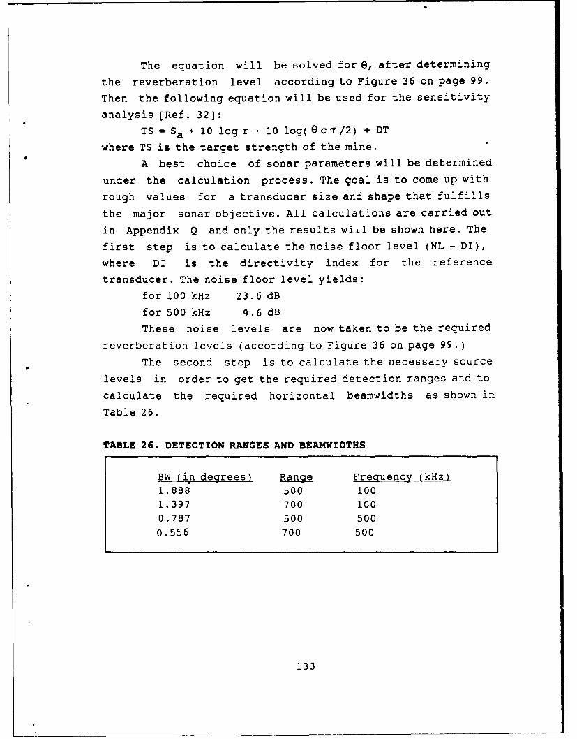
The equation will be solved for e, after determiningthe reverberation level according to Figure 36 on page 99.

Then the following equation will be used for the sensitivity

analysis [Ref. 32]:

TS = Sa + 10 log r + 10 log(ec-/2) + DT

where TS is the target strength of the mine.

A best choice of sonar parameters will be determined

under the calculation process. The goal is to come up with

rough values for a transducer size and shape that fulfills

the major sonar objective. All calculations are carried out

in Appendix Q and only the results will be shown here. The

first step is to calculate the noise floor level (NL - DI),

where DI is the directivity index for the reference

transducer. The noise floor level yields:

for 100 kHz 23.6 dB

for 500 kHz 9.6 dB

These noise levels are now taken to be the required

reverberation levels (according to Figure 36 on page 99.)

The second step is to calculate the necessary source

levels in order to get the required detection ranges and to

calculate the required horizontal beamwidths as shown in

Table 26.

TABLE 26. DETECTION RANGES AND BEAMWIDTHS

BW (in degrees) Range Frequency (kHz'1.888 500 1001.397 700 1000.787 500 5000.556 700 500

133

Noting that the reference transducer gives horizontal

beamwidths of 1.397 degrees for 100 kHz and 0.556 degrees

for 500 kHz we can conclude that satisfying the sonarsrequired range, is possible. In addition, given the decrease

in sonar size requirements, other objectives, simple

logistics and low cost, for example; become possible once

the carrier frequency is determined. Since 100 kHz givesbeamwidth values that makes the transducer sizes reasonable,

this lower frequency is preferred from a hardware point ofview. Further, since the primary goal is to detect a mine at

a distance of 700 meters, a 1.397 degrees beamwidth is

acceptable.

The third step is to vary the target strength versus

beamwidth, and to make a conclusion of a realistic target

strength, using parameters from a "real" mine. From the

calculations in Appendix Q, pages 4 and 5, a target strengthof +5 dB is determined. A beamwidth of 4.423 degrees is then

adequate, which means that the circular transducer can be

reduced from a diameter of 1 meter to 0.22 meters. The

necessary SL and DI will now change to 168.5 dB and 33.3 dB.

The horizontal beamwidth requirement has now been met,

but the vertical beamwidth is left to be considered. Thesection on multipath propagation indicates that the vertical

beamwidth must be at least 25 degrees in order to utilize

all the direct paths to the target (considering the whole

year). Since a circular transducer creates a pencil beam,

this will not give an appropriate beam pattern. There is apossibility, of course, to use a pencil beam and then scanthrough the required search volume both vertically and

horizontally. This takes time however, and the scan time

must be made as short as possible. The original reason for

choosing a circular transducer was a trade off between

maximum transducer size (1 meter), practical handling and

sonar dome shape. Since the sizes now turn out to be much

134

smaller, a planar array or aperture is an option. The

advantage of a planar aperture is that a vertical beamwidth

of 25 degrees is possible to achieve, together with a narrow

horizontal beamwidth (fan beam). The following approximate

equations can be used to calculate the planar aperture.

[Ref. 32]

BW(v) = ,/LI

BW(h) =X./L2

where BW(h) = horizontal beamwidth

BW(v) = vertical beamwidth

Ll = transducer widthL2 = transducer length

For the beamwidths above, a rectangular planar

transducer will measure a length of 0.2 meters and a width

of 0.04 meters. The new values for the directivity index and

source level yields 25.5 dB and 176.3 dB.

The next question is, "Is it possible to transmit a SL

of 176.3 dB with that aperture size due to the cavitation

threshold?" When a transducer is excited, cavitation bubbles

are developed on the front of the transducer.

"These bubbles are a manifestation of the rupture of thewater caused by the negative pressures of the generatedsound field. These neqative pressures tear the liquidapart, so to speak, when they exceed a certain valuecalled the cavitation threshold.' [Ref. 9:p. 76]

The cavitation threshold can be calculated using the

following equation [Ref. 9]:

Ic = 0.3 * p W/cm 2

where Ic = cavitation threshold, W/cm 2

p = peak pressure of sound wave causing cavitation

(in atm)

135

The p value is determined by Urick [Ref. 9:Figure 4.6]

for 100 kHz to be 2 atm (worst case). This gives a

cavitation threshold of 1.2 W/cm 2 . With a transducer area

of 80 cm2, the maximum power is 96 W. Using the following

equation solves for the source level:

SL = 10 log P + DI + 171 re 1 Pa

where P = power in W

With a DI of 25.5 dB re 1 Pa, the maximum source

level will be 216 dB. Since the required source level is far

under this level, the bubble cavitation is not a problem.

The calculations above have utilized the limiting

value for the reverberation which occurs when the echo

changes from being masked by noise to being masked by

reverberation. Increasing the power further will not

influence the range but only emphasize the reverberation

limited performance. In an actual design it might be

advisable to increase the SL for hardware reasons since a SL

of 176.3 dB gives very low power values (0.01 W).

F. TRANSDUCER STUDY

The transducer can be designed as a planar array or a

planar aperture. The advantage of using an array technique

is that FFT beamforming and beamsteering can be utilized and

the array itself need not to be scanned inside the dome. An

array consist of many small transducer elements which must

be amplitude and phase weighted together. This implies a

more sophisticated signal processing technique. One

disadvantage, in this case, is that the wavelength is only

0.015 meters for 100 kHz. When considering beamsteering with

an array, the transducer elements must be spaced at a

distance less then 1/2 wavelength in order to avoid grating

lobes. This means that the element spacing must be less than

0.0075 meters. Narrow spacing can give unwanted radiation

coupling between the elements. Also, in order for the

136

elements to act like point sources (which makes the beampattern prediction easier), the element length must be smallcompared to a wavelength. In this case this means fractionsof a millimeter. These facts makes a choice of a steerable

array technique very difficult to pursue. However, an arraytechnique might still be utilized in an unsteerable mode;where no phase weighting is performed. To simplify thecalculations a planar aperture is chosen for the further

transducer design.

The directivity function of a planar aperture can becalculated by taking the two dimensional spatial Fouriertransformation of the transducer aperture function. Theaperture function is the frequency response of the planaraperture, when it is excited by an input electrical signal.The directivity function is simply the beam pattern of thetransducer. The aperture function is normally a complexfunction, but since, in this case, no beam steering will beused, only the amplitude window (real part) needs to beconsidered. There are many different amplitude windows tochose from and only a few of them have a closed formsolution. It is important in probably all sonar designs tosuppress the sidelobes in order to minimize the effects ofnoise and other unwanted signals. The design then becomes atrade off between the beamwidth and the sidelobe level(SLL), since normally suppressing the sidelobes broadens thebeamwidth. A broadening of the mainbeam must be compensatedwith larger aperture size. Since the size in the design is

relatively small, an increase in transducer size isrecommended to get low sidelobes. Therefore a Blackmanwindow is chosen as the amplitude window function. Thischoice results in a sidelobe suppression of -58 dB. A one

dimensional Blackman amplitude window function is given by

the expression:

137

a(flx)=(0.42 + 0.5 cos(@ x/L) + 0.08 cos(4 x/L)) rect(L)

where x = transducer in the x direction, i.e., a linear

aperture

L = length of the aperture

rect(L) = rectangular window, i.e., a constant.

This one dimensional case can be extended into two

dimensions, i.e., a planar aperture. The development of a

planar aperture directivity function is shown in Appendix R.

The problems to physically manufacture an aperture with a

Blackman window response will not be discussed here.

In order to compute the beam pattern, the measurements of

the aperture must first be computed. The aperture size can

be determined by using the following equation:

:= 2sin [ u]

where Au = 3dB beamwidth in direction cosine space

4= horizontal beamwidth (in this case)

and A u = 1.6444X/L

where L = transducer length

Using this equation with the required horizontal and

vertical beamwidths yields an aperture width of 0.319 meters

and a height of 0.057 meters. The directivity index (DI) and

the required source level stay approximately the same, that

is 25.5 dB and 176.3 dB, since the mainlobe beamwidths have

not been changed.

In order to make sure that the target is in the far

field, the range to the far field must be computed. The

following equation can be used [Ref. 33]:

138

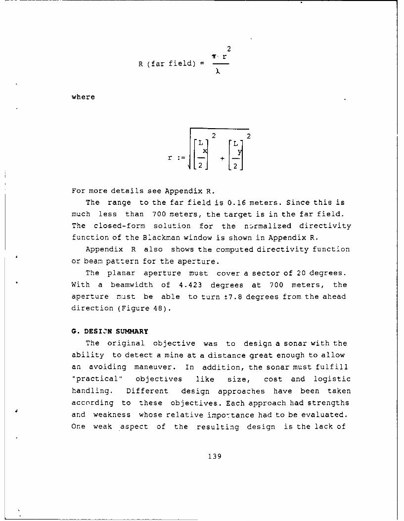
2T. r

R (far field) -

where

2

r+

For more details see Appendix R.

The range to the far field is 0.16 meters. Since this is

much less than 700 meters, the target is in the far field.

The closed-form solution for the normalized directivity

function of the Blackman window is shown in Appendix R.

Appendix R also shows the computed directivity function

or beam pattern for the aperture.

The planar aperture must cover a sector of 20 degrees.

With a beamwidth of 4.423 degrees at 700 meters, the

aperture must be able to turn ±7.8 degrees from the ahead

direction (Figure 48).

G. DESIGN SUMMARY

The original objective was to design a sonar with the

ability to detect a mine at a distance great enough to allow

an avoiding maneuver. In addition, the sonar must fulfill"practical" objectives like size, cost and logistic

handling. Different design approaches have been taken

according to these objectives. Each approach had strengths

and weakness whose relative impo-tance had to be evaluated.

One weak aspect of the resulting design is the lack of

139

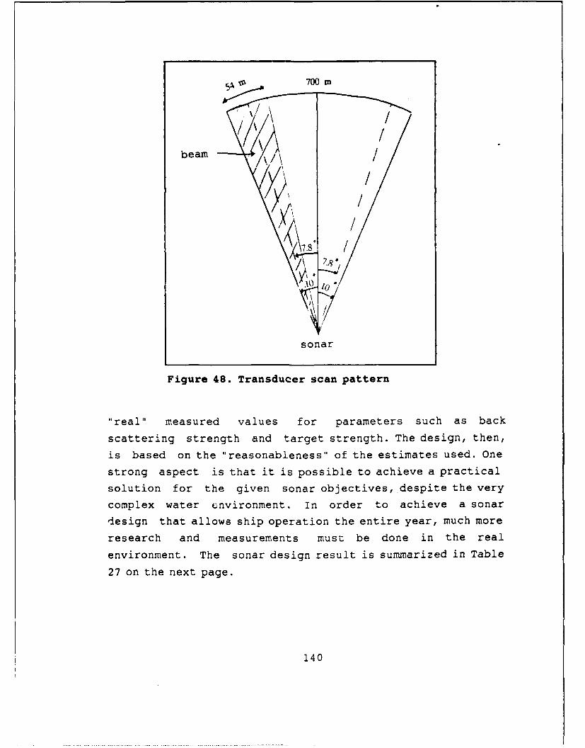
700 m

beam

.1

sonar

Figure 48. Transducer scan pattern

"real" measured values for parameters such as back

scattering strength and target strength. The design, then,

is based on the "reasonableness" of the estimates used. One

strong aspect is that it is possible to achieve a practical

solution for the given sonar objectives, despite the very

complex water environment. In order to achieve a sonar

design that allows ship operation the entire year, much more

research and measurements must be done in the real

environment. The sonar design result is summarized in Table

27 on the next page.

140

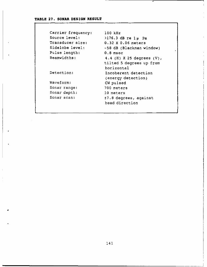
TABLE 27. SONAR DESIGN RESULT

Carrier frequency: 100 kHzSource level: >176.3 dB re IV PaTransducer size: 0.32 X 0.06 metersSidelobe level: -58 dB (Blackman window)Pulse length: 0.8 msecBeamwidths: 4.4 (H) X 25 degrees (V),

tilted 5 degrees up fromhorizontal

Detection: Incoherent detection

(energy detection)Waveform: CW pulsedSonar range: 700 metersSonar depth: 10 metersSonar scan: ±7.8 degrees, against

head direction

141

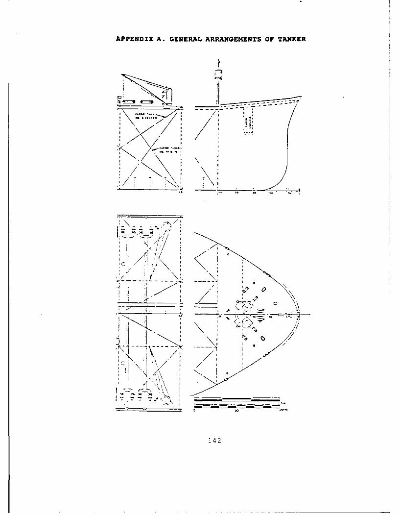
APPENDIX A. GENERAL ARRANGEMENTS OF TANKER

CI - - -- ~~

~

I j

I * 3,

S --- a

I,

n,..~I I

I I? I

4IS ,,. Jo - .- =D

V ~;$4

~ I

/ I

_____________ I -~

I ~. -~.. - >

0 "-~--- 4

I II I -,

7/i'~ A' I

~'~-$~: I ~ -

-a--

142

APPENDIX A (page 2)

. - .. ...

---

..,. --- -. ,.- T -

.... ....-

.1

/3

APPENDIX B. CRASH STOP AHEAD TEST

-.. 70.- c.--'..- 2 w-q -

- ~ ~ ~ ~ ~ ~ ~ ~ ~ ~ ~ I' ------ --- . .--- -- - - . - -- r, AZ... A-- -

____Y.- 2T

J:I

44.. . . . . . . .

APPENDIX C. CRASH STOP ASTERN TEST

14 5

APPENDIX D. MODIFIED ZIP-ZAG TEST

'D I. S i~.j~

- , D7G--Z aN ) E 8 h,

I rfk 4j A A6 FT, zsi- "

A..i~ A 1~3

- -- 46

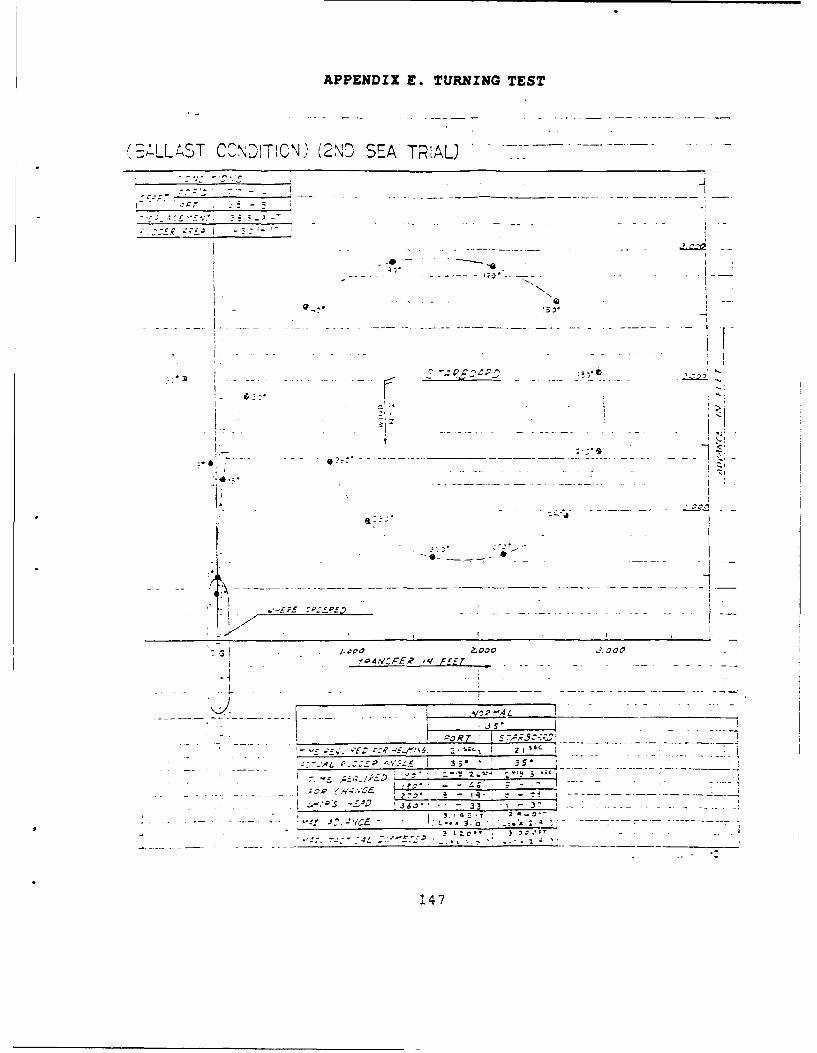
APPENDIX E. TURNING TEST

t= AL LAST CCN-DITICN) (2%,D" SEA T2IAL) -

I60 33 3

14 7

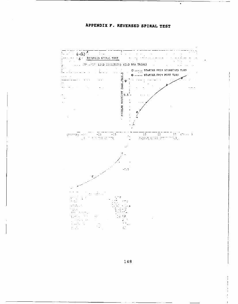
APPENDIX F. REVERSED SPIRAL TEST

- -- -- O..f c:::Ut:;) (::iD SF.A TR.AL).

0 ... --- 0 STAR70D FRO:I S7A'RBC.%FR' T,:R,!

0)... STAR. ~lFP.O PCRT TUR-'

41,

7)-

14

APPENDIX G. ECK ORGANIZATION

= ~

-~ = = ~= .~

- I- I

-= ~ -~- -=

- ~

.- ~ C,, -

* I

___________

-- ~*-, -- - i**, - -

- =

49

APPENDIX H. CALCULATION OF PULSE DENSITY

:-et the he-- of the emi:ter and the EM antenna be

h z= I

7he raiar i n. imted ::3S

2 .3 ) h i.e. R - 25 km

The 3eparati:n bet-een ships at sea is assumed to average

:: 5 nm

sep

..ence the t.-tal nu-mber of ships within L.OS is

N~~ [_ ie. 25L dsep T

:f the fraztizn cf ships that are military is

f : = . 1

Then the n-:.-.-er -f :=vilian and military ships are

- and N11 f NSTM T

7he r. ber :. radars assu.ing one per civilian ship and two per militaryship

: z .e. n 27R C M

There are also c:astal radars and long range radars

2 RN and N 2::st i km iong

For the short, med *.-n and long ranges, we can determine the PPRs form.axm ra.e with:-t an-i.b .ui ty. Let the various ranses be

( i 1I . .' )

150

APPENDIX H (page 2)

Then t.-e c:rreZpndin9 ??s are determined from:

2 -1 c 1 £

1 2 Rmi H

7he n.m.er :f radars in each range type (I - short, 3 - long) are

n N * N N n := N and n N.1, coast 2 M 3 l ng

The n' mer =f r a:ars in eazh category are

n

n 5

Anr the -"7s in eaz: radar range category are

n F

g ?=T :E2;7 5z

151

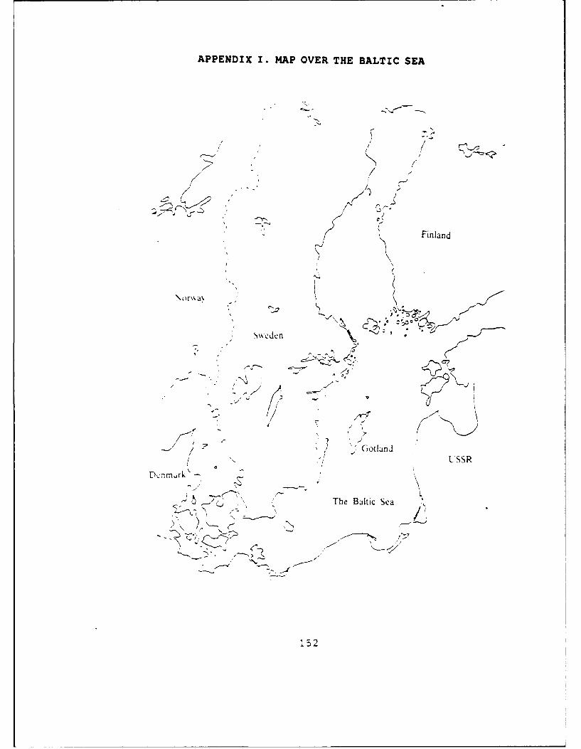
APPENDIX I. MAP OVER THE BALTIC SEA

- -, A

Finland

Nor\\a\

-. e-

-Ji ? } -i' Gotland

jI

". USSR

D , nim a r k "

.' The Baltic Sea '-15 2

- - " --. <-._2 -<--> " 7

? 52

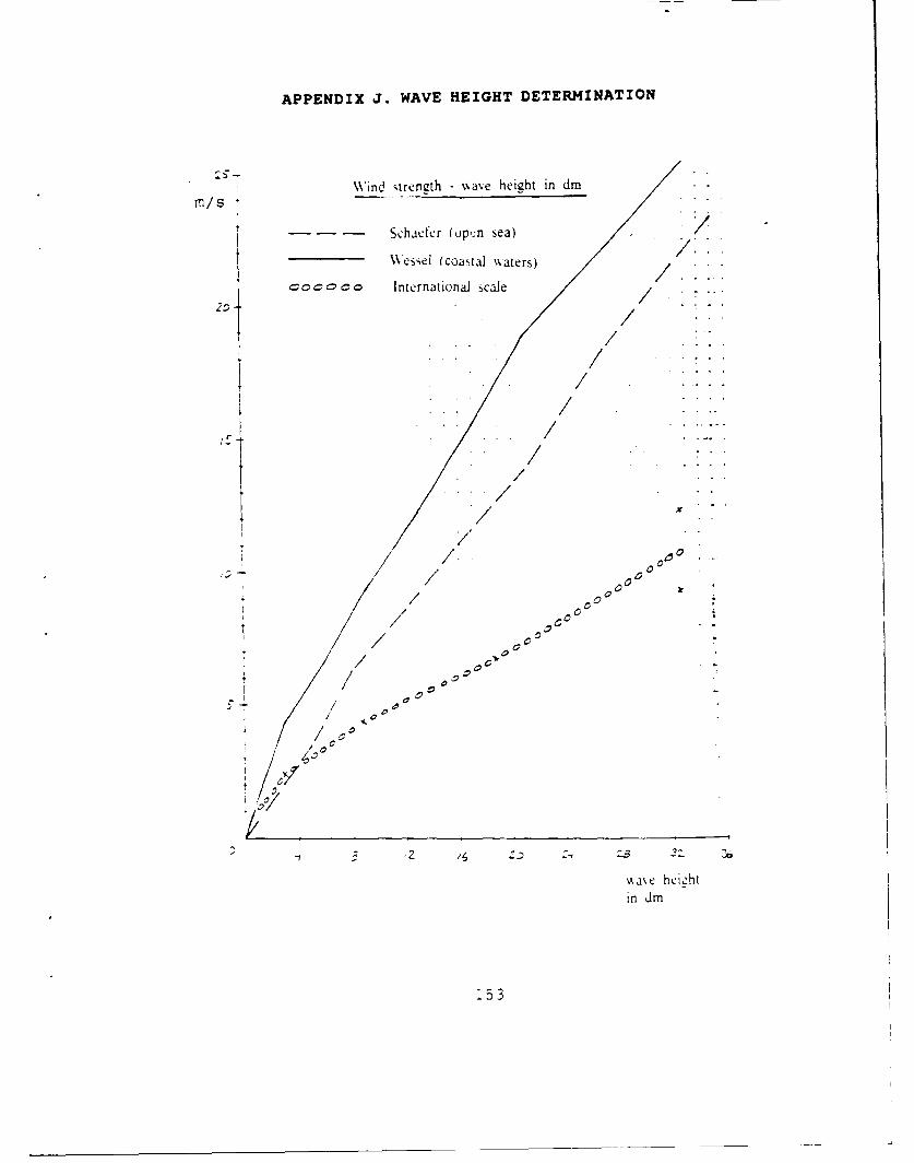
APPENDIX J. WAVE HEIGHT DETERMINATION

Wind strength -%,,ave height in dmm/S

- - - Schaefer (upcn sea)

\\cssel (coastal waters)/

-- International scale /

00 coo

:- /3 2' 3

* / o

, /I/

%kate heirohi

in dmn

5 3

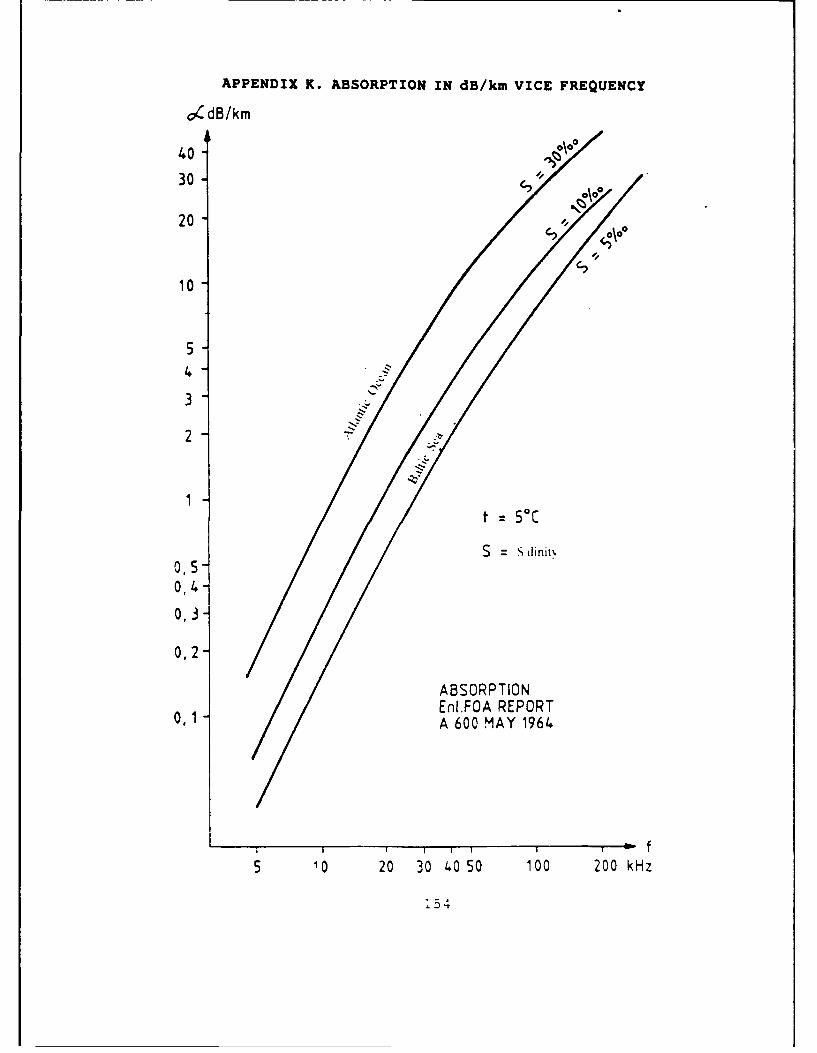
APPENDIX K. ABSORPTION IN dB/km VICE FREQUENCY

ddB/km

4030 ,,

20 C, C,

10

54 -

3

2

1 t =5°C

S = S dinit'\0,50,4-

0, .3

0, 2

ABSORPTIONEnI.FOA REPORT

0, 1 A 600 MAY 1964

I I I I f

5 10 20 30 40 50 100 200 kHz

154

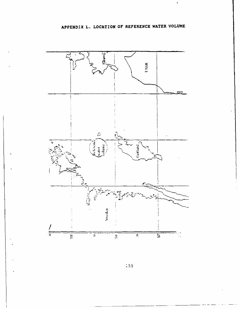
APPENDIX L. LOCATION OF REFERENCE WATER VOLUME

155

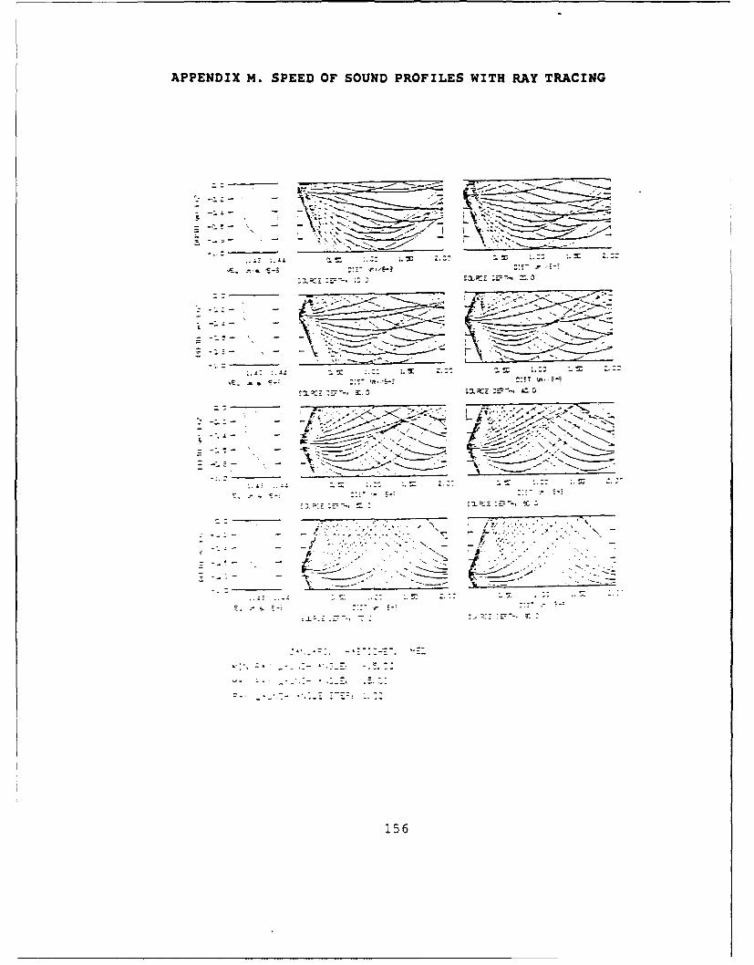
APPENDIX M. SPEED OF SOUND PROFILES WITH RAY TRACING

''Cr

156-~ -

APPENDIX M (page 2)

...-.. - - --7- - ..

. _- ,, - -

7

-_ ....- --

= -- .-- . -\ . . -. : "' - J --

- -: _- -- - .

t\

* / '" - - '-- , A, -.' .

- .- , "..+

-- -._ E --- ' _ _ _

i57

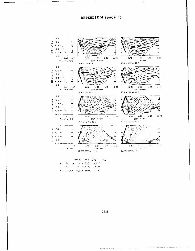
APPENDIX M4 (page 3)

r .7s

~a T

- - C*:F--;

-I z

- ~Z. 7:

.. .. ... .. ..

APPENDIX M (page 4)

-- 7 - -

* - - N

- - ---159

APPENDIX M (page 5)

-: . ' S: - _ ,c C . 5 *1 ..C:

-12 -

;- . -- - - - -

'E / :,- S /

r.-' .' .. .3 .- - " -0& , C S, -3

- _ s .,. _-.. . . ;,

_, . - - - - -_ - - / --. _._. ".--V .., .. -

*, -,. .- , ..-.-'.-__3

:.7, -- - - 5-

i - - - i""160

'. ' ' _ - ' " T-- -'. . .

• ,- /-...-=.., _._ . - ,', _E -Z_ : : "N

*- .60

APPENDIX M (page 6.)

-x-- - i

r . ,. "_ I ,.' ,

... .. _ . - N.. _ _-.

- :- " - .. : - '...,Z- -r

- - -. v. )' . ; , -- .

-- _ . , j--S I-- - '. -. lAA At L ,-

161

APPENDIX M (page 7)

.- ~7.

45" -

- , Z

50 1.7 '. Z

3r '3;C

-----------

____ ___ ___ ___ 7162*

APPENDIX M (page 8)

.2\" "7 I-

__ - - N

-:-'A- - , -t '-

--- - ..--'.- -O Z .

-_ __ ______. _ _______ _ ._--.

S .. . - ". 5.. •5.. - -

-o/ _- Z -7

""' : '.. - ". _E' - . . - -"". -

'63

APPENDIX H (page 9)

- -*:.j\ "

. - --

\ N

* -- \ -.

_': - .-=: - - --

164

APPENDIX M (page 10)

AtC. 5: i;

VE 1a- c-5-

- - - 3- fr\Z

5:.5

APPENDIX M (page 11)

At.,--

N N

I A I.IL

7

5Z. 7. Z.5:Z

7,L

166~

APPENDIX M (page 12)

~

-- -- -~- .

'vs.- -

-- A- - -~

-- ~-------~. --z -~- -..- - ~- ~-~-----~ S

--- N-.-

'4 -... -.-

___________ ~. -.- '----

- - . . --~ - I" -. -

- -

.. .

p

167

APPENDIX N. BOTTOM REFLECTION COEFFICIENT DIAGRAM

d=g rad18o

k : 0 .. ,9rl : 1440000rZ :7953000

C! 1440C2 1500

ktdec

S deq*0 de'5 deg-0 dea:5 deg10 dea5 dea

60 de45decl

55 deg

.7 4de

Cie:

L decl

[c2 ]CL K]]

k r2 osI16

168

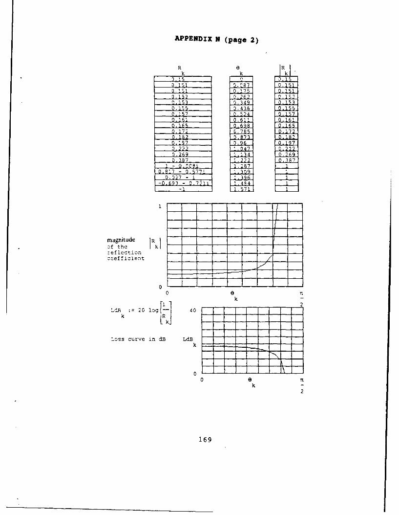
APPENDIX N (page 2)

R Rk k

0.151 0.0870.151 0.17 5

7* 153 .62r0.153 0.349 0. C _

.75 o1 77 A 7.s 0.43 7.5

0.22 151 7, ,4 ,

o.i61 0,1 0.1l ,1

0.165 09698 0 50.172 0.785 0,1720.182 0.873o~ig-0.197 0.96 0.,1970,222 1, 470,2220,269 .1,134 0.2 690,387 1,222o.38?t

- 7*0TI 1.80.8!7 - 0.577i _,309

0.027 - i 1.3960.693 - 0.721i ' 4-4

magnitude RkCf the k

reflectioncoefficient

0 e V

k

J2U 20 log~- 40 ----

Loss curve in dB LdBk

0 81k

2

169

APPENDIX 0. KNUDSEN'S CURVES FOR AMBIENT NOISE

\z

///

II /I

- 1/1/I /. / Ii/I I/,..,

Cl C> -

6rr

170

1'70

APPENDIX P. MISC. CURVES AND DIAGRAMS

9999 I A / 1 ,i

09

50.0

10

coo, i-----

o001 31005, 2 10 mo;50 0 g0 98,995 199990 01 01 0'2 I 5 Z0 40 60 80 95 99 999 99999

14-

10.

2 5 10 .1C 50 ?00i(N ' r of -mcepede, %. -s

171

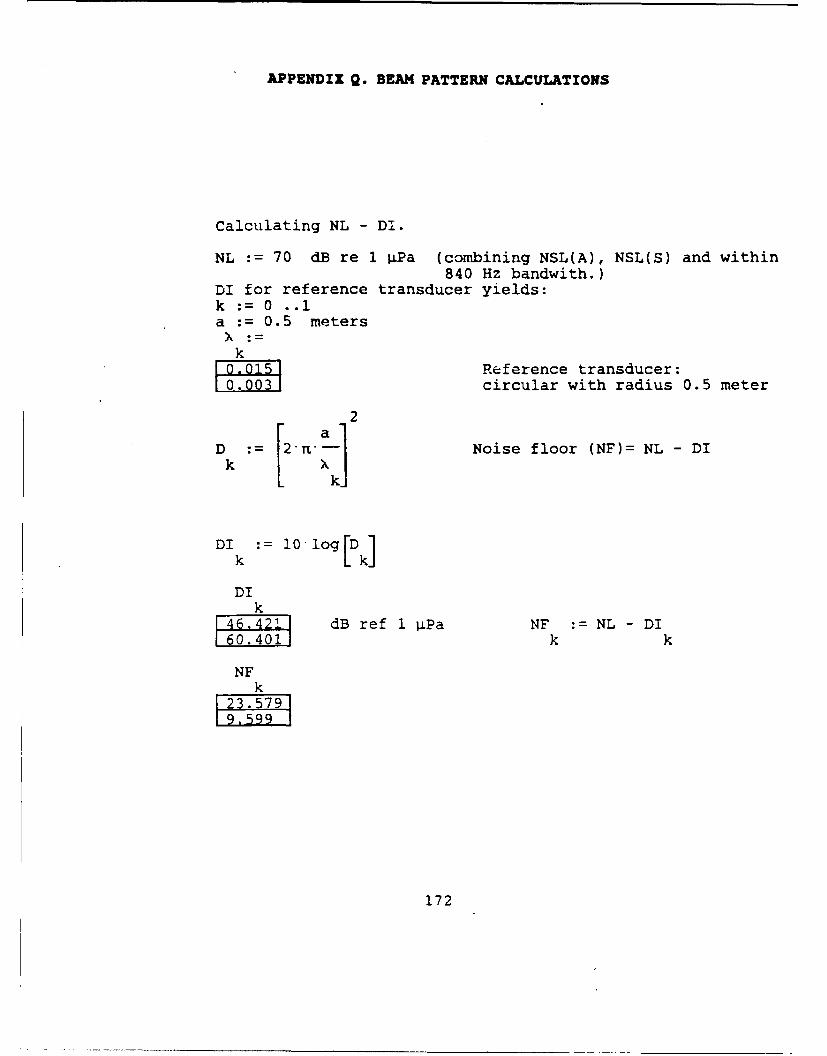
APPENDIX Q. BEAM PATTERN CALCULATIONS

Calculating NL - DI.

NL := 70 dB re 1 iPa (combining NSL(A), NSL(S) and within840 Hz bandwith.)

DI for reference transducer yields:k :=0 ..la := 0.5 meters

k.Reference transducer:

circular with radius 0.5 meter

2

D =n- Noise floor (NF)= NL - DIk

DIk 10 log[ Dk

DIk

dB ref 1 iPa NF :NL -DIk k

NFk

23.57919.5997

172

APPENDIX Q (page 2)

Determining the Source Level (SL)

SL = RL + 2*TL - TS + DTk := 0 .. 3RL:= r := a TS:

k k k k79 100 kHz

100 kHz9.599 5 500 kHz9.599 100500 kHz

rk

[20 l [r ] k

SL :RL + 2" 0"log + a - - TS + 9k SL k k 1000 k

SLk*SL for 100 kHz and 500 m range

SL for 100 kHz and 700 m rangeE 8 SL for 500 kHz and 500 m rangeSL for 500 kHz and 700 m range

173

APPENDIX Q (page 3)

Determining the horizontal beamwith.Using expression for surface reverberation in ref [341 p.425.

k := 0 ..3

RL SL TL SA Rk k k k k23,579 15,3 58.9 -19.11 50 100 kHz

23.579 160 363.2 -100 kHz9,599 22 8104 -11 500 kHz

9.599 272.4031 126.9 -15.1 500 kHz

RL -SL +2 TL -SA -10 log k

e(k) := 1.67-10

180BW :e(k)'

k it

BW Beam widths in degrees fork

100 kHz and range 500 m100 kHz and range 700 m500 kHz and range 500 m500 kHz and range 700 m

174

APPENDIX Q (page 4)

Sensitivity analysis; Varying the TS toinvestigate the performance limitations.

k -25 ..12 Target Strength variation

SA -19.1 Scattering strength

DT 9 Detection threshold

k-SA-DT-10 log(700)

109 k) 1.67 10

180BWk) 9(k) - Beamwidth in degrees

It

30 20 1 1

Bw(k) - B w(k)

,0 5 k 15 -10 k 10

a 0 .9

k Bw k3 a .

T~rge Beamw~dth inStrength degrees

175

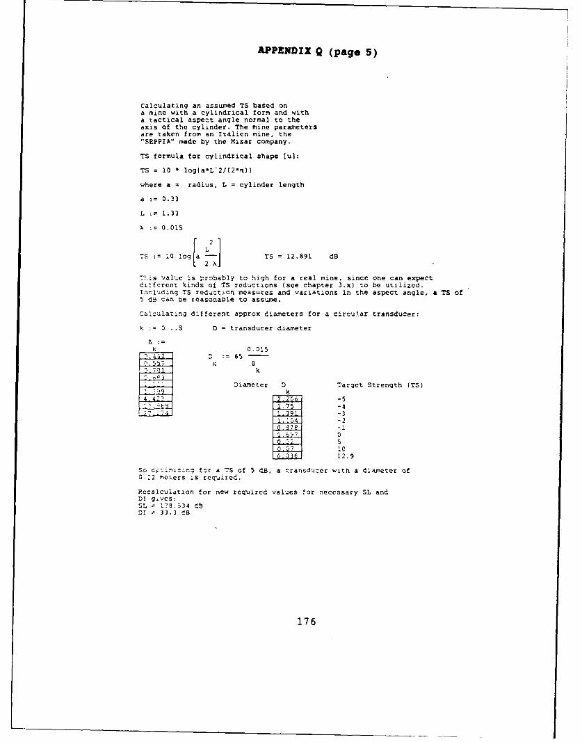
APPENDIX Q (page 5)

Calculating an assumed TS based ona mine with a cylindrical form and witha tactical aspect angle normal to theaxis of the cylinder. The mine parametersare taken from an Italien mine, the"SEPPIA" made by the Misar company.

TS formula for cylindrical shape (u):

TS = 10 t log(a*L'2/(2*n))

where a radius, L = cylinder length

a 0.33

L 1.33

0.015

TS 10 log[a -j TS = 12.891 dB

This value is probably to high for a real mine, since one can expectdiffcrent kinds of TS reductions (see chapter 3.x) to be utilized.Iarluding TS reduction measures and variations in the aspect angle, a TS ofS d5 can be reasonable to assume.

Calculating different approx diameters for a circular transducer:

kI 0 ..3 D = transducer diameter

k 0.01511 := 65 -

57k Bk

Diameter D Target Strength (TS)-.99 k

4,42"2.2C6-5

-3-2

I.8 -i

0

12.9

So c i~iz~n for a TS of 5 dB, a transduier with a diameter of0.:2 meters is required.

Recalculation for new required values for necessary SL andDI givcs:SL = 1?8.534 dSDI = 33.3 dB

176

APPENDIX R. BEAMWIDTH CALCULATIONS

Calculating horizontal and vertical beam pattern for a planar aperture witha Blackman a:-Tlitude window.The aperture tunction for a planar aperture with separable functions (theaperture function can be written as a product of two functions) and withBlackman amplitude weighting used for both functions yields:

A(fx,y) = Black(Lx) * Black(Ly)

he normalized directivity function or beam pattern yields:

D(f,fx,fy) = Dx(f,fx) * D(ffy)

Calculating horizontal beampattern: (set v = 0,(see next page) which0.0!5 yields D(f,fy" 1 ) ,Z:=0.02.5

u -1,-0.999 ..i

fx(u) : - here u = sin e * cost

L :z 0.319 //gY

n(f,fx.fy) = D)x(f,fx) gives:

11.68 - 0.18 (L fx(u)) ]sin( L'fx(u))D~u)

0.42 riL fx(u) (L fx(u)) 1 [(L fx(u)) - 4]

-1 uWhere u (dircction cosinus) = sin e * sin

177

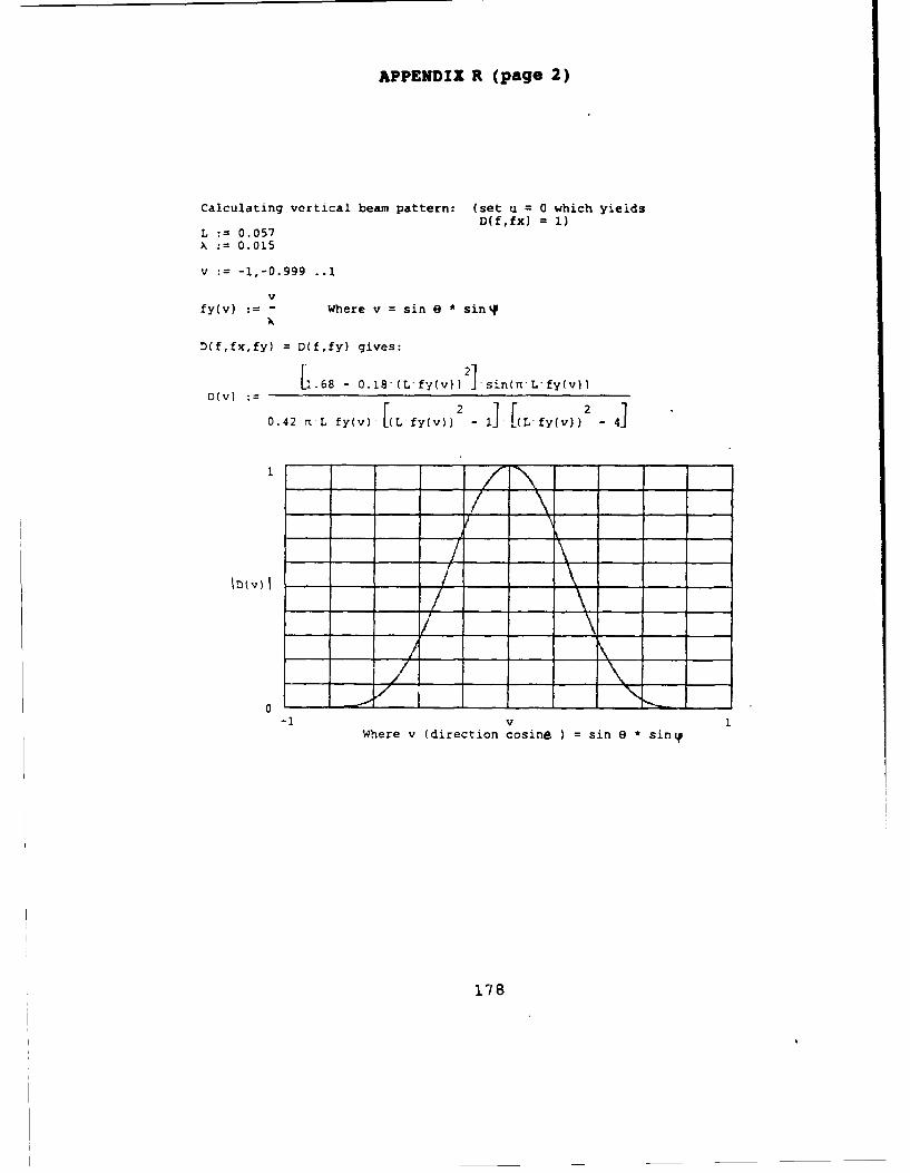
APPENDIX R (page 2)

Calculating vertical beam pattern: (set u = 0 which yieldsD(f,fx) = 1)

L : 0.057X : 0.015

v -1,-0.999 ..1

fy(v) : - Where v = sin e * sin%?

D(f,fx,fy) = D(f,fy) gives:

1.68 - 0.18(Lfy(v)) sin(n'L'fy(v)lD(v) :

0.42 n L fy(v) [(L fy(v)) - 1i [(Lfy(v)) - 4]

-1 vWhere v (direction cosine ) = sin e ) siny

178

LIST OF REFERENCES

1. The Scandinavian Shipping Gazette, SjofartensBok, 1989.

2. Michel, Walter H., The Mission Impact on VesselDesign, from Ship Design and Construction 1980,Society of Naval Architects and MaritimeEngineers, 1980.

3. Chevron Transport Corp., San Francisco CA, USA.

4. Skolnik Merril I., Introduction to Radar Systems,McGraw'Aill, 1980.

5. U.S. Naval Research Laboratory, Washington, D.C.6. Ottosson, R., MHS Kompendium i Radar, Tele and

Telemotmedel Teknik, MHS Stockholm, 1984.7. Coppens klan B., Sanders James V., and Dahl,

Harve A., "Introduction to the Sonar Equations,"Tex at erial to Physics Course at NavalPostgraduate School, Monterey, CA, 1982

8. Cox, Albert W., Sonar and Underwater Sound,Lexington Books, 1974.

9. Urick, Robert J., Principles of Underwater Sound,3d edition, McGraw-Hill Book Company, 1983.

10. Burdic, William S., Underwater Acoustic SystemAnalysis, Prentice-Hall, Inc., 1984.

11. Kihlman, T. and Plunt, J., Prediction of NoiseLevels in Ships, International Symposium onShipboard Acoustics, 1976.

12. Brown,. Neal A., Cavitation Noise Problems andSolutions, International Symposium on ShipboardAcoustics, 1976.

13. Cybulski J. Probable Origin of MeasuredSupertanker kadiated Noise Spectra, Ocean'77Conference Record, 1977.

14. Gillier, Thomas C. and Johnson, BruceIntroduction to Naval Architecture, 4 avalInstitute Press, 1987.

15. Skudrzyk, E.J., and Haddle, G.P, Noise Productionin a Turbulent Boundary Layer by Smooth and RoughSurfaces, J. Acoust. Soc. Am. 32, page 19, Jan.1960.

16. Chaff for Ships: Operatio:2al Considerations,International Countermeasures Handbook, 1981.

179

17. Gunston, Bill, Modern Airborne Missiles,Prentice Hall Press, 1986.

18. Schleher, Curtis. Introduction to ElectronicWarfare, Artech House Inc., 1986.

19. Short Course Electronic Warfare, EW qroup, NavalPostgraduate School, Monterey CA, USA.

20. Van Brunt, Leroy, Applied ECM, Vol 1., 1978.

21. Product Data Sheets, Plessey Microwave, VA, 198722. Friedman, Norman, The Offboard Countermeasures,

1988.

23. Baranauskas, Tom Anti-Ship Missile Threat DrivesDecoy Development, Defense Electronics, March1988.

24. Boyd,J.A., Harris, D.B., King, D.D. and WelchH.W. Jr., Electronic Countermeasures, PeninsulaPublishing, 1978.

25. Blanchard, Benjamin S. and Fabrycky, Wolter J.,Systems Engineering and Analysis, rentice-Hall,Inc., 1981.

26. Sonobuoy Instruction Manual, Direction ofCommander, Naval Air Systems Command, USA, 1988.

27. Tsui James Bao-Yen Microwave Receivers withElectronic Warfare Applications, 1986.

28. Bonniers Albert Bonniers 3-band lexikon,forlag, Sweden, 1970.

29. Svensk Lots del A (Swedish Pilot Guide),Sjofartsverket Sweden, 1985.

30. FMV, Swedish Defense Material Administration,Stockholm, Sweden.

31. Sveriges Geologiska Undersokning (GeologicalSurvey) Maringeologiska kartan Serie Am nr 1,SGU, 19d7.

32. Kinsler, Lawrence E., Frey, Austin R., Coppens,Alan B., and Sanders, James V., Fundamentals ofAcoustics, John Wiley and Sons, 1984.

33. Ziomek, Lawrence J., Underwater Acoustics,Academic Press, Inc., 1985.

34. Ingham, A.E Hydrography for the Surveyor andEngineer, BSP Professlonal Books, 1984.

35. FOA rapport C 30289-El, Activt ParametrisktHydrofonsystem, Pentelius Tore, Aug 1982.

36. FOA, Forsvarets Forskningsanstalt (Swedish DefenseResearch Establishment), Stockholm, Sweden

37. Wibaeus, Sten, Sonarteknik, Teleplan, 1985.

38. Kroenert J.T., J. Acoust. Soc. Am. 71(2), page 507,Feb. 1982.

180

39. Sackman Georqe L., High Resolution Sonar ConceptFormulafion, Naval Postgraduate School, Monterey,CA, 1979.

40. Hecht, Eugene, Optics (second edition),Addison-Wesley Publishing Company, 1980.

41. Urick, Robert J. Sound Propagation in the Sea,Peninsula Publishing, 1982.

42. Clay, Clarence S. and Medwin, Herman AcousticalOceanography, John Wiley and Sons, 1977

43. J. Geoph. Res., 71 2037 Clay, C.S, CoherentRelection of SoundFrom 'he ocean Bottom, 1966.

44. B. Aktiva hydrofonsystem, FQA rapport C 30168-ElBetydelsen av havets transmissionsegenskaper viakonstruktion av hydroakustiska system, Pentelius,Tore, Nov 1979.

181

BIBLIOGRAPHY

Electronic Warfare -- The Future, Navy InternationalMarch 1984.

The Falklands Campaign: The Lesson, Her Majesty'sStationary Office, 1972.

FOA 3 rapport C 3680-El Pentelius, Tore, LiudvagorsReflexion Mot Skiktad Havsbotten Med Speciel Hansyn TillOstersjoforhallanden, Aug 1971.

Norweqian Council for Technical and Scientific Research,Report B.0930.4502.1, Noise Control in Ships, 1985.

Ratcliffe, Mike Liquid Gold Ship, Lloyd's of LondonPress Ltd., 1975.

Skolnik, Merril I., Radar Handbook, McGraw'Hill, 1970.

SSPA, Maritime Consulting. Gothenburg, Sweden.

Van Brunt, Leroy B., Applied ECM, Vol 2., 1982.

Wiseman, Charles H., Chaff Assists Anti-Ship MissileDefence, EW: July/August 1977.

182

• I I I I I III

INITIAL DISTRIBUTION LIST

1. Defense Technical Information Center 2Cameron StationAlexandria, Virginia 22304-6145

2. Library, Code 0142 2Naval Postgraduate SchoolMonterey, California 93943-5002

3. MHS MarinlinjenValhallavagen 117Box 80007104 50 StockholmSWEDEN

4. Chairman, Code 73Department of Electronic WarfareNaval Postgraduate SchoolMonterey, California 93943-5000

5. Chairman, Code 61 AyDepartment of PhysicsNaval Postgraduate SchoolMonterey, California 93943-5000

6. Prof. L. Partelow11 Paseo De VaquerosSalinas, California 93908

7. Prof. A. Coppens, Code 61 C2Department of PhysicsNaval Postgraduate SchoolMonterey, California 93943-5000

183