Embed Size (px)
Citation preview
Natural Sciences Tripos Part IB
Mathematical Methods I
Michaelmas 2016
Dr Henrik Latter
Contents
1 Vector calculus 1
1.1 Motivation . . . . . . . . . . . . . . . . . . . . . . . . . 1
1.2 Suffix notation and Cartesian coordinates . . . . . . . . . 1
1.2.1 Three-dimensional Euclidean space . . . . . . . . 1
1.2.2 Properties of the Cartesian unit vectors . . . . . . 2
1.2.3 Suffix notation . . . . . . . . . . . . . . . . . . . 3
1.2.4 Delta and epsilon . . . . . . . . . . . . . . . . . 4
1.2.5 Einstein summation convention . . . . . . . . . . 5
1.2.6 Matrices and suffix notation . . . . . . . . . . . . 6
1.2.7 Product of two epsilons . . . . . . . . . . . . . . 7
1.3 Vector differential operators . . . . . . . . . . . . . . . . 9
1.3.1 The gradient operator . . . . . . . . . . . . . . . 9
1.3.2 Geometrical meaning of the gradient . . . . . . . 10
1.3.3 Related vector differential operators . . . . . . . . 12
1.3.4 Vector invariance . . . . . . . . . . . . . . . . . . 14
i

CONTENTS ii
1.3.5 Vector differential identities . . . . . . . . . . . . 15
1.4 Integral theorems . . . . . . . . . . . . . . . . . . . . . . 17
1.4.1 The gradient theorem . . . . . . . . . . . . . . . 17
1.4.2 The divergence theorem (Gauss’s theorem) . . . . 17
1.4.3 The curl theorem (Stokes’s theorem) . . . . . . . 22
1.4.4 Geometrical definitions of grad, div and curl . . . 24
1.5 Orthogonal curvilinear coordinates . . . . . . . . . . . . . 25
1.5.1 Line element . . . . . . . . . . . . . . . . . . . . 25
1.5.2 The Jacobian . . . . . . . . . . . . . . . . . . . . 26
1.5.3 Properties of Jacobians . . . . . . . . . . . . . . 28
1.5.4 Orthogonality of coordinates . . . . . . . . . . . . 28
1.5.5 Commonly used orthogonal coordinate systems . . 30
1.5.6 Vector calculus in orthogonal coordinates . . . . . 33
1.5.7 Grad, div, curl and ∇2 in cylindrical and spherical
polar coordinates . . . . . . . . . . . . . . . . . . 36
2 Partial differential equations 38
2.1 Motivation . . . . . . . . . . . . . . . . . . . . . . . . . 38
2.2 Linear PDEs of second order . . . . . . . . . . . . . . . . 38
2.2.1 Definition . . . . . . . . . . . . . . . . . . . . . 38
2.2.2 Principle of superposition . . . . . . . . . . . . . 39
2.2.3 Classic examples . . . . . . . . . . . . . . . . . . 40
2.3 Physical examples of occurrence . . . . . . . . . . . . . . 40
2.3.1 Examples of Laplace’s (or Poisson’s) equation . . 40
2.3.2 Examples of the diffusion equation . . . . . . . . 41
2.3.3 Examples of the wave equation . . . . . . . . . . 44
2.3.4 Examples of other second-order linear PDEs . . . 45
CONTENTS iii
2.3.5 Examples of nonlinear PDEs . . . . . . . . . . . . 45
2.4 Separation of variables (Cartesian coordinates) . . . . . . 46
2.4.1 Diffusion equation . . . . . . . . . . . . . . . . . 46
2.4.2 Wave equation (example) . . . . . . . . . . . . . 48
2.4.3 Helmholtz equation (example) . . . . . . . . . . . 50
3 Green’s functions 52
3.1 Impulses and the delta function . . . . . . . . . . . . . . 52
3.1.1 Physical motivation . . . . . . . . . . . . . . . . 52
3.1.2 Step function and delta function . . . . . . . . . 53
3.2 Other definitions . . . . . . . . . . . . . . . . . . . . . . 54
3.3 More on generalized functions . . . . . . . . . . . . . . . 57
3.4 Differential equations containing delta functions . . . . . 57
3.5 Inhomogeneous linear second-order ODEs . . . . . . . . . 60
3.5.1 Complementary functions and particular integral . 60
3.5.2 Initial-value and boundary-value problems . . . . . 60
3.5.3 Green’s function for an initial-value problem . . . 61
3.5.4 Green’s function for a boundary-value problem . . 66
3.6 Unlectured remarks . . . . . . . . . . . . . . . . . . . . 69
4 The Fourier transform 70
4.1 Motivation . . . . . . . . . . . . . . . . . . . . . . . . . 70
4.2 Fourier series . . . . . . . . . . . . . . . . . . . . . . . . 71
4.3 Approaching the Fourier transform . . . . . . . . . . . . 72
4.4 Examples . . . . . . . . . . . . . . . . . . . . . . . . . . 77
4.5 Basic properties of the Fourier transform . . . . . . . . . 80
4.6 The delta function and the Fourier transform . . . . . . . 83
4.7 The convolution theorem . . . . . . . . . . . . . . . . . 84
CONTENTS iv
4.7.1 Definition of convolution . . . . . . . . . . . . . . 84
4.7.2 Interpretation and examples . . . . . . . . . . . . 84
4.7.3 The convolution theorem . . . . . . . . . . . . . 86
4.7.4 Correlation . . . . . . . . . . . . . . . . . . . . . 87
4.8 Parseval’s theorem . . . . . . . . . . . . . . . . . . . . . 88
4.9 Power spectra . . . . . . . . . . . . . . . . . . . . . . . 90
5 Matrices and linear algebra 92
5.1 Motivation . . . . . . . . . . . . . . . . . . . . . . . . . 92
5.2 Vector spaces . . . . . . . . . . . . . . . . . . . . . . . 92
5.2.1 Abstract definition of scalars and vectors . . . . . 92
5.2.2 Span and linear dependence . . . . . . . . . . . . 94
5.2.3 Basis and dimension . . . . . . . . . . . . . . . . 95
5.2.4 Examples . . . . . . . . . . . . . . . . . . . . . . 96
5.2.5 Change of basis . . . . . . . . . . . . . . . . . . 97
5.3 Matrices . . . . . . . . . . . . . . . . . . . . . . . . . . 98
5.3.1 Array viewpoint . . . . . . . . . . . . . . . . . . 98
5.3.2 Linear operators . . . . . . . . . . . . . . . . . . 99
5.3.3 Change of basis again . . . . . . . . . . . . . . . 101
5.4 Inner product (scalar product) . . . . . . . . . . . . . . . 102
5.4.1 Definition . . . . . . . . . . . . . . . . . . . . . 102
5.4.2 The Cauchy–Schwarz inequality . . . . . . . . . . 103
5.4.3 Inner product and bases . . . . . . . . . . . . . . 105
5.5 Hermitian conjugate . . . . . . . . . . . . . . . . . . . . 106
5.5.1 Definition and simple properties . . . . . . . . . . 106
5.5.2 Relationship with inner product . . . . . . . . . . 107
5.5.3 Adjoint operator . . . . . . . . . . . . . . . . . . 108

CONTENTS v
5.5.4 Special square matrices . . . . . . . . . . . . . . 108
5.6 Eigenvalues and eigenvectors . . . . . . . . . . . . . . . 109
5.6.1 Basic properties . . . . . . . . . . . . . . . . . . 109
5.6.2 Eigenvalues and eigenvectors of Hermitian matrices 111
5.6.3 Related results . . . . . . . . . . . . . . . . . . . 112
5.6.4 The degenerate case . . . . . . . . . . . . . . . . 114
5.7 Diagonalization of a matrix . . . . . . . . . . . . . . . . 116
5.7.1 Similarity . . . . . . . . . . . . . . . . . . . . . . 116
5.7.2 Diagonalization . . . . . . . . . . . . . . . . . . 117
5.7.3 Diagonalization of a normal matrix . . . . . . . . 117
5.7.4 Orthogonal and unitary transformations . . . . . . 118
5.7.5 Uses of diagonalization . . . . . . . . . . . . . . 119
5.8 Quadratic and Hermitian forms . . . . . . . . . . . . . . 120
5.8.1 Quadratic form . . . . . . . . . . . . . . . . . . . 120
5.8.2 Quadratic surfaces . . . . . . . . . . . . . . . . . 122
5.8.3 Hermitian form . . . . . . . . . . . . . . . . . . . 125
5.9 Stationary property of the eigenvalues . . . . . . . . . . . 125
6 Elementary analysis 127
6.1 Motivation . . . . . . . . . . . . . . . . . . . . . . . . . 127
6.2 Sequences . . . . . . . . . . . . . . . . . . . . . . . . . 127
6.2.1 Limits of sequences . . . . . . . . . . . . . . . . 127
6.2.2 Cauchy’s principle of convergence . . . . . . . . . 128
6.3 Convergence of series . . . . . . . . . . . . . . . . . . . 129
6.3.1 Meaning of convergence . . . . . . . . . . . . . . 129
6.3.2 Classic examples . . . . . . . . . . . . . . . . . . 129
6.3.3 Absolute and conditional convergence . . . . . . . 130
CONTENTS vi
6.3.4 Necessary condition for convergence . . . . . . . . 131
6.3.5 The comparison test . . . . . . . . . . . . . . . . 131
6.3.6 D’Alembert’s ratio test . . . . . . . . . . . . . . 132
6.3.7 Cauchy’s root test . . . . . . . . . . . . . . . . . 133
6.4 Functions of a continuous variable . . . . . . . . . . . . . 133
6.4.1 Limits and continuity . . . . . . . . . . . . . . . 133
6.4.2 The O notation . . . . . . . . . . . . . . . . . . 135
6.5 Taylor’s theorem for functions of a real variable . . . . . . 136
6.6 Analytic functions of a complex variable . . . . . . . . . . 137
6.6.1 Complex differentiability . . . . . . . . . . . . . . 137
6.6.2 The Cauchy–Riemann equations . . . . . . . . . . 137
6.6.3 Analytic functions . . . . . . . . . . . . . . . . . 138
6.6.4 Consequences of the Cauchy–Riemann equations . 140
6.7 Taylor series for analytic functions . . . . . . . . . . . . . 141
6.8 Zeros, poles and essential singularities . . . . . . . . . . . 142
6.8.1 Zeros of complex functions . . . . . . . . . . . . 142
6.8.2 Poles . . . . . . . . . . . . . . . . . . . . . . . . 143
6.8.3 Laurent series . . . . . . . . . . . . . . . . . . . 145
6.8.4 Behaviour at infinity . . . . . . . . . . . . . . . . 146
6.9 Convergence of power series . . . . . . . . . . . . . . . . 146
6.9.1 Circle of convergence . . . . . . . . . . . . . . . 146
6.9.2 Determination of the radius of convergence . . . . 147
6.9.3 Examples . . . . . . . . . . . . . . . . . . . . . . 148
7 Ordinary differential equations 149
7.1 Motivation . . . . . . . . . . . . . . . . . . . . . . . . . 149
7.2 Classification . . . . . . . . . . . . . . . . . . . . . . . . 149

CONTENTS vii
7.3 Homogeneous linear second-order ODEs . . . . . . . . . . 150
7.3.1 Linearly independent solutions . . . . . . . . . . . 150
7.3.2 The Wronskian . . . . . . . . . . . . . . . . . . . 151
7.3.3 Calculation of the Wronskian . . . . . . . . . . . 151
7.3.4 Finding a second solution . . . . . . . . . . . . . 152
7.4 Series solutions . . . . . . . . . . . . . . . . . . . . . . . 154
7.4.1 Ordinary and singular points . . . . . . . . . . . . 154
7.4.2 Series solutions about an ordinary point . . . . . . 155
7.4.3 Series solutions about a regular singular point . . 160
7.4.4 Irregular singular points . . . . . . . . . . . . . . 164
CONTENTS 8
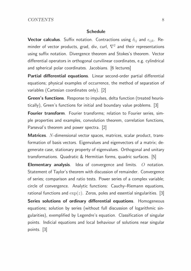
Schedule
Vector calculus. Suffix notation. Contractions using δij and ǫijk. Re-
minder of vector products, grad, div, curl, ∇2 and their representations
using suffix notation. Divergence theorem and Stokes’s theorem. Vector
differential operators in orthogonal curvilinear coordinates, e.g. cylindrical
and spherical polar coordinates. Jacobians. [6 lectures]
Partial differential equations. Linear second-order partial differential
equations; physical examples of occurrence, the method of separation of
variables (Cartesian coordinates only). [2]
Green’s functions. Response to impulses, delta function (treated heuris-
tically), Green’s functions for initial and boundary value problems. [3]
Fourier transform. Fourier transforms; relation to Fourier series, sim-
ple properties and examples, convolution theorem, correlation functions,
Parseval’s theorem and power spectra. [2]
Matrices. N -dimensional vector spaces, matrices, scalar product, trans-
formation of basis vectors. Eigenvalues and eigenvectors of a matrix; de-
generate case, stationary property of eigenvalues. Orthogonal and unitary
transformations. Quadratic & Hermitian forms, quadric surfaces. [5]
Elementary analysis. Idea of convergence and limits. O notation.
Statement of Taylor’s theorem with discussion of remainder. Convergence
of series; comparison and ratio tests. Power series of a complex variable;
circle of convergence. Analytic functions: Cauchy–Riemann equations,
rational functions and exp(z). Zeros, poles and essential singularities. [3]
Series solutions of ordinary differential equations. Homogeneous
equations; solution by series (without full discussion of logarithmic sin-
gularities), exemplified by Legendre’s equation. Classification of singular
points. Indicial equations and local behaviour of solutions near singular
points. [3]
CONTENTS 9
Course websites
http://www.student-systems.admin.cam.ac.uk/moodle
NST Part IB: Mathematics
www.damtp.cam.ac.uk/user/hl278/NST
Assumed knowledge
I will assume familiarity with the following topics at the level of Course A
of Part IA Mathematics for Natural Sciences.
• Algebra of complex numbers
• Algebra of vectors (including scalar and vector products)
• Algebra of matrices
• Eigenvalues and eigenvectors of matrices
• Taylor series and the geometric series
• Calculus of functions of several variables
• Line, surface and volume integrals
• The Gaussian integral
• First-order ordinary differential equations
• Second-order linear ODEs with constant coefficients
• Fourier series

CONTENTS 10
Textbooks
The following textbooks are recommended. The first grew out of the NST
Maths course, so it will be particularly close to the lectures in places.
• K. F. Riley, M. P. Hobson and S. J. Bence (2006). Mathematical
Methods for Physics and Engineering, 3rd edition. Cambridge Univer-
sity Press
• G. Arfken and H. J. Weber (2005). Mathematical Methods for Physi-
cists, 6th edition. Academic Press
Questions
• Please ask questions in lecture, especially brief ones (typos, jargon)
• Longer questions can be e-mailed to me: [email protected]. Turnaround
time: approximately 1-3 days

1 VECTOR CALCULUS 1
1 Vector calculus
1.1 Motivation
Scientific quantities are of different kinds:
• scalars have only magnitude (and sign), e.g. mass, electric charge,
energy,
temperature
• vectors have magnitude and direction, e.g. velocity, magnetic field,
temperature gradient
A field is a quantity that depends continuously on position (and possibly
on time). Examples:
• air pressure in this room (scalar field)
• electric field in this room (vector field)
Vector calculus is concerned with scalar and vector fields. The spatial vari-
ation of fields is described by vector differential operators, which appear
in the partial differential equations governing the fields.
Vector calculus is most easily done in Cartesian coordinates, but other
systems (curvilinear coordinates) are better suited for many problems be-
cause of symmetries or boundary conditions.
1.2 Suffix notation and Cartesian coordinates
1.2.1 Three-dimensional Euclidean space
This is a close approximation to our physical space:
• points are the elements of the space
• vectors are translatable, directed line segments

1 VECTOR CALCULUS 2
• Euclidean means that lengths and angles obey the classical results of
geometry
Points and vectors have a geometrical existence without reference to any
coordinate system. For definite calculations, however, we must introduce
coordinates.
Cartesian coordinates:
• measured with respect to an origin O and a system of orthogonal axes
Oxyz
• points have coordinates (x, y, z) = (x1, x2, x3)
• unit vectors (ex, ey, ez) = (e1, e2, e3) in the three coordinate direc-
tions, also called (ı, , k) or (x, y, z)
The position vector of a point P is
−→OP = r = exx+ eyy + ezz =
3∑
i=1
eixi
1.2.2 Properties of the Cartesian unit vectors
The unit vectors form a basis for the space. Any vector a belonging to
the space can be written uniquely in the form
a = exax + eyay + ezaz =3
∑
i=1
eiai
where ai are the Cartesian components of the vector a.
The basis is orthonormal (orthogonal and normalized):
e1 · e1 = e2 · e2 = e3 · e3 = 1
e1 · e2 = e1 · e3 = e2 · e3 = 0
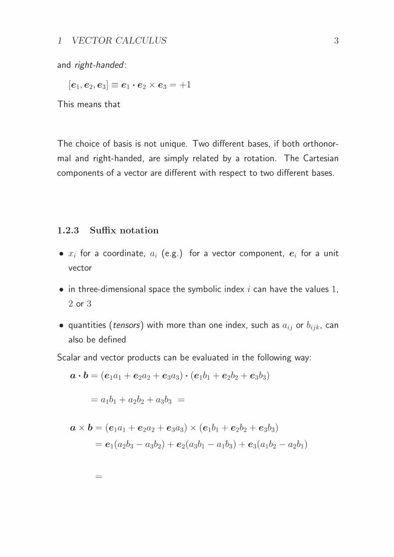
1 VECTOR CALCULUS 3
and right-handed :
[e1, e2, e3] ≡ e1 · e2 × e3 = +1
This means that
e1 × e2 = e3 e2 × e3 = e1 e3 × e1 = e2
The choice of basis is not unique. Two different bases, if both orthonor-
mal and right-handed, are simply related by a rotation. The Cartesian
components of a vector are different with respect to two different bases.
1.2.3 Suffix notation
• xi for a coordinate, ai (e.g.) for a vector component, ei for a unit
vector
• in three-dimensional space the symbolic index i can have the values 1,
2 or 3
• quantities (tensors) with more than one index, such as aij or bijk, can
also be defined
Scalar and vector products can be evaluated in the following way:
a · b = (e1a1 + e2a2 + e3a3) · (e1b1 + e2b2 + e3b3)
= a1b1 + a2b2 + a3b3 =3
∑
i=1
aibi
a× b = (e1a1 + e2a2 + e3a3)× (e1b1 + e2b2 + e3b3)
= e1(a2b3 − a3b2) + e2(a3b1 − a1b3) + e3(a1b2 − a2b1)
=
∣
∣
∣
∣
∣
∣
∣
∣
e1 e2 e3
a1 a2 a3
b1 b2 b3
∣
∣
∣
∣
∣
∣
∣
∣

1 VECTOR CALCULUS 4
1.2.4 Delta and epsilon
Suffix notation is made easier by defining two symbols. The Kronecker
delta symbol is
δij =
1 if i = j
0 otherwise
In detail:
δ11 = δ22 = δ33 = 1
all others, e.g. δ12 = 0
δij gives the components of the unit matrix. It is symmetric :
δji = δij
and has the substitution property :
3∑
j=1
δijaj = ai (in matrix notation, 1a = a)
The Levi-Civita permutation symbol is
ǫijk =
1 if (i, j, k) is an even permutation of (1, 2, 3)
−1 if (i, j, k) is an odd permutation of (1, 2, 3)
0 otherwise
In detail:
ǫ123 = ǫ231 = ǫ312 = 1
ǫ132 = ǫ213 = ǫ321 = −1
all others, e.g. ǫ112 = 0
1 VECTOR CALCULUS 5
An even (odd) permutation is one consisting of an even (odd) number of
transpositions (interchanges of two neighbouring objects). Therefore ǫijk
is totally antisymmetric : it changes sign when any two indices are inter-
changed, e.g. ǫjik = −ǫijk. It arises in vector products and determinants.
ǫijk has three indices because the space has three dimensions. The even
permutations of (1, 2, 3) are (1, 2, 3), (2, 3, 1) and (3, 1, 2), which also
happen to be the cyclic permutations. So ǫijk = ǫjki = ǫkij.
Then we can write
a · b =3
∑
i=1
aibi =3
∑
i=1
3∑
j=1
δijaibj
a× b =
∣
∣
∣
∣
∣
∣
∣
∣
e1 e2 e3
a1 a2 a3
b1 b2 b3
∣
∣
∣
∣
∣
∣
∣
∣
=3
∑
i=1
3∑
j=1
3∑
k=1
ǫijkeiajbk
1.2.5 Einstein summation convention
The summation sign is conventionally omitted in expressions of this type.
It is implicit that a repeated index is to be summed over. Thus
a · b = aibi
and
a× b = ǫijkeiajbk or (a× b)i = ǫijkajbk
The repeated index should occur exactly twice in any term. Examples of
invalid notation are:
a · a = a2i (should be aiai)
(a · b)(c · d) = aibicidi (should be aibicjdj)
The repeated index is a dummy index and can be relabelled at will. Other
indices in an expression are free indices. The free indices in each term in
an equation must agree.

1 VECTOR CALCULUS 6
Examples:
a = b ai = bi
a = b× c ai = ǫijkbjck
|a|2 = b · c aiai = bici = bjcj
a = (b · c)d+ e× f ai = bjcjdi + ǫijkejfk
Contraction is an operation by which we set one free index equal to an-
other, so that it is summed over. For example, the contraction of aij is
aii. Contraction is equivalent to multiplication by a Kronecker delta:
aijδij = a11 + a22 + a33 = aii
The contraction of δij is δii = 1 + 1 + 1 = 3 (in three dimensions).
If the summation convention is not being used, this should be noted
explicitly.
1.2.6 Matrices and suffix notation
Matrix (A) times vector (x):
y = Ax yi = Aijxj
Matrix times matrix:
A = BC Aij = BikCkj
Transpose of a matrix:
(AT)ij = Aji
Trace of a matrix:
trA = Aii
Determinant of a (3× 3) matrix:
detA = ǫijkA1iA2jA3k
(or many equivalent expressions).
1 VECTOR CALCULUS 7
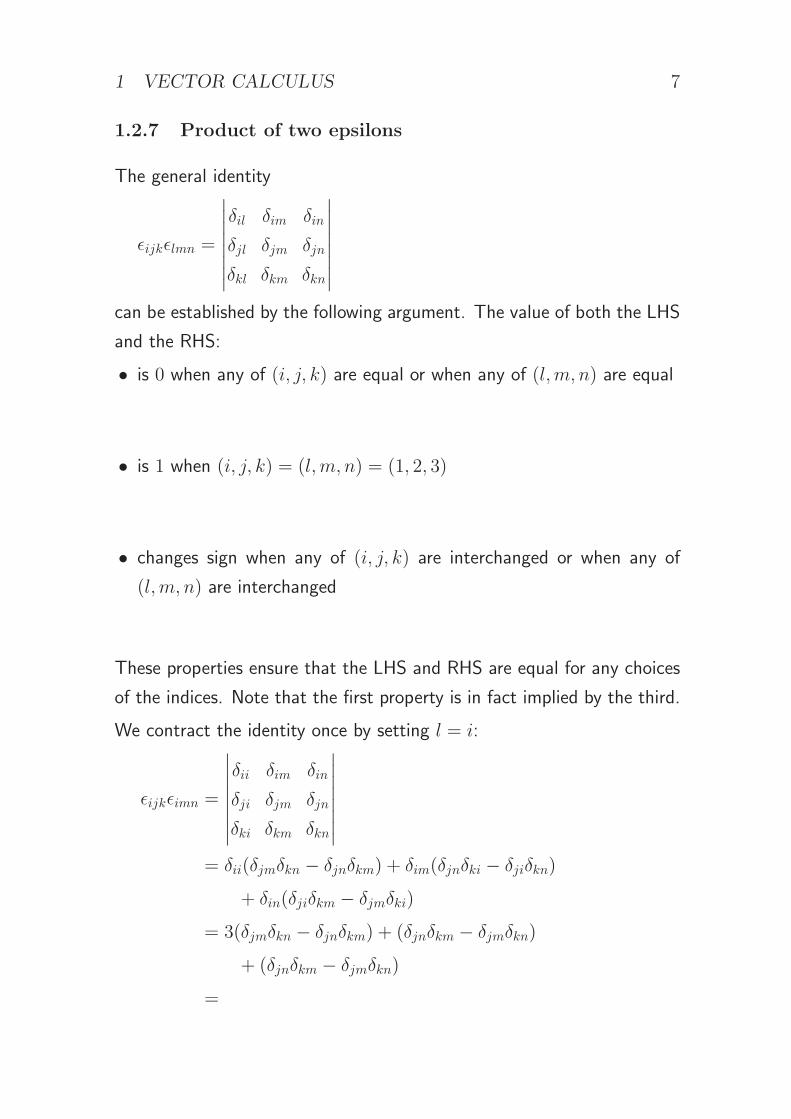
1.2.7 Product of two epsilons
The general identity
ǫijkǫlmn =
∣
∣
∣
∣
∣
∣
∣
∣
δil δim δin
δjl δjm δjn
δkl δkm δkn
∣
∣
∣
∣
∣
∣
∣
∣
can be established by the following argument. The value of both the LHS
and the RHS:
• is 0 when any of (i, j, k) are equal or when any of (l,m, n) are equal
• is 1 when (i, j, k) = (l,m, n) = (1, 2, 3)
• changes sign when any of (i, j, k) are interchanged or when any of
(l,m, n) are interchanged
These properties ensure that the LHS and RHS are equal for any choices
of the indices. Note that the first property is in fact implied by the third.
We contract the identity once by setting l = i:
ǫijkǫimn =
∣
∣
∣
∣
∣
∣
∣
∣
δii δim δin
δji δjm δjn
δki δkm δkn
∣
∣
∣
∣
∣
∣
∣
∣
= δii(δjmδkn − δjnδkm) + δim(δjnδki − δjiδkn)
+ δin(δjiδkm − δjmδki)
= 3(δjmδkn − δjnδkm) + (δjnδkm − δjmδkn)
+ (δjnδkm − δjmδkn)
= δjmδkn − δjnδkm

1 VECTOR CALCULUS 8
This is the most useful form to remember:
ǫijkǫimn = δjmδkn − δjnδkm
Given any product of two epsilons with one common index, the indices
can be permuted cyclically into this form, e.g.:
ǫαβγǫµνβ = ǫβγαǫβµν = δγµδαν − δγνδαµ
Further contractions of the identity:
ǫijkǫijn = δjjδkn − δjnδkj
= 3δkn − δkn
= 2δkn
ǫijkǫijk = 6
Example . . . . . . . . . . . . . . . . . . . . . . . . . . . . . . . . . . . . . . . . . . . . . . . . . . . . . . . . . . . .
⊲ Show that (a× b) · (c× d) = (a · c)(b · d)− (a · d)(b · c).
(a× b) · (c× d) = (a× b)i(c× d)i
= (ǫijkajbk)(ǫilmcldm)
= ǫijkǫilmajbkcldm
= (δjlδkm − δjmδkl)ajbkcldm
= ajbkcjdk − ajbkckdj
= (ajcj)(bkdk)− (ajdj)(bkck)
= (a · c)(b · d)− (a · d)(b · c)
. . . . . . . . . . . . . . . . . . . . . . . . . . . . . . . . . . . . . . . . . . . . . . . . . . . . . . . . . . . . . . . . . . . .
1 VECTOR CALCULUS 9
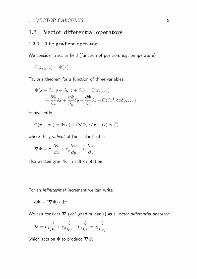
1.3 Vector differential operators
1.3.1 The gradient operator
We consider a scalar field (function of position, e.g. temperature)
Φ(x, y, z) = Φ(r)
Taylor’s theorem for a function of three variables:
Φ(x+ δx, y + δy, z + δz) = Φ(x, y, z)
+∂Φ
∂xδx+
∂Φ
∂yδy +
∂Φ
∂zδz +O(δx2, δxδy, . . . )
Equivalently
Φ(r + δr) = Φ(r) + (∇Φ) · δr +O(|δr|2)
where the gradient of the scalar field is
∇Φ = ex∂Φ
∂x+ ey
∂Φ
∂y+ ez
∂Φ
∂z
also written gradΦ. In suffix notation
∇Φ = ei∂Φ
∂xi
For an infinitesimal increment we can write
dΦ = (∇Φ) · dr
We can consider ∇ (del, grad or nabla) as a vector differential operator
∇ = ex∂
∂x+ ey
∂
∂y+ ez
∂
∂z= ei
∂
∂xi
which acts on Φ to produce ∇Φ.
1 VECTOR CALCULUS 10
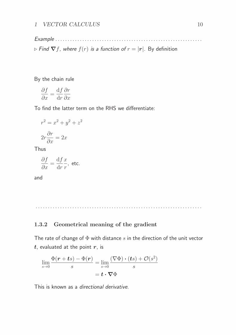
Example . . . . . . . . . . . . . . . . . . . . . . . . . . . . . . . . . . . . . . . . . . . . . . . . . . . . . . . . . . . .
⊲ Find ∇f , where f(r) is a function of r = |r|. By definition
∇f = ex∂f
∂x+ ey
∂f
∂y+ ez
∂f
∂z
By the chain rule
∂f
∂x=
df
dr
∂r
∂x
To find the latter term on the RHS we differentiate:
r2 = x2 + y2 + z2
2r∂r
∂x= 2x
Thus
∂f
∂x=
df
dr
x
r, etc.
and
∇f =df
dr
(x
r,y
r,z
r
)
=df
dr
r
r
. . . . . . . . . . . . . . . . . . . . . . . . . . . . . . . . . . . . . . . . . . . . . . . . . . . . . . . . . . . . . . . . . . . .
1.3.2 Geometrical meaning of the gradient
The rate of change of Φ with distance s in the direction of the unit vector
t, evaluated at the point r, is
lims→0
Φ(r + ts)− Φ(r)
s= lim
s→0
(∇Φ) · (ts) +O(s2)
s
= t · ∇Φ
This is known as a directional derivative.
1 VECTOR CALCULUS 11
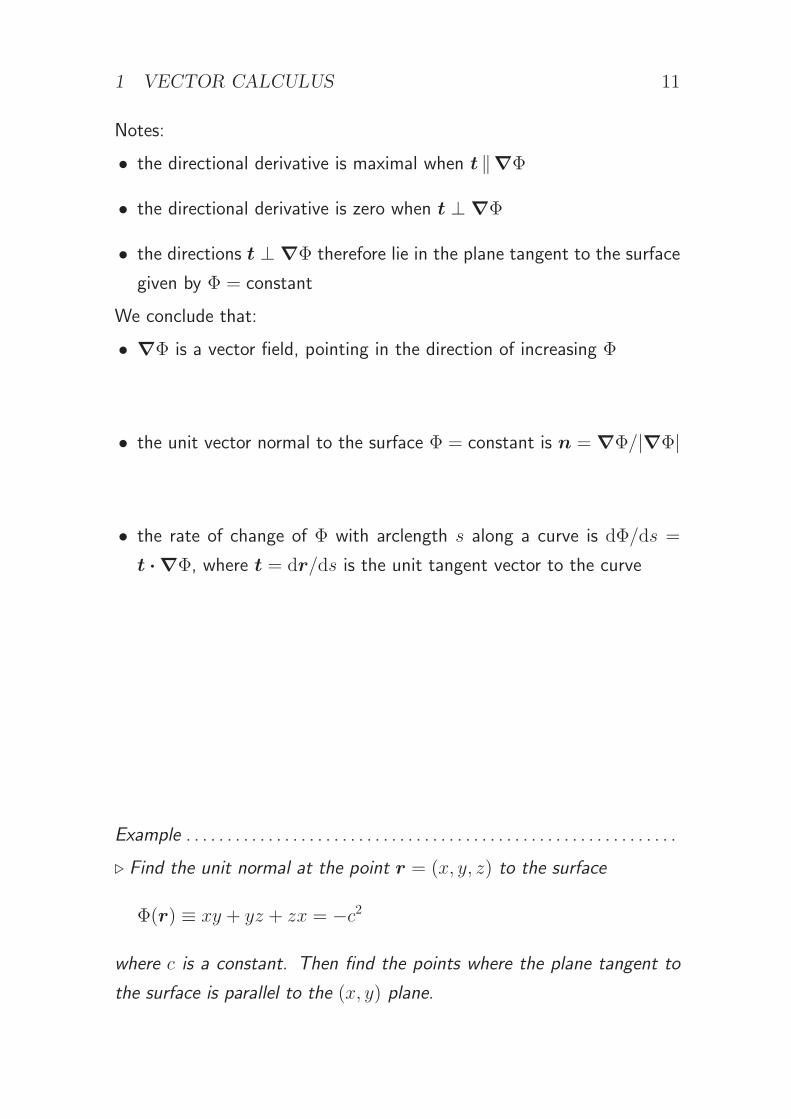
Notes:
• the directional derivative is maximal when t ‖∇Φ
• the directional derivative is zero when t ⊥ ∇Φ
• the directions t ⊥ ∇Φ therefore lie in the plane tangent to the surface
given by Φ = constant
We conclude that:
• ∇Φ is a vector field, pointing in the direction of increasing Φ
• the unit vector normal to the surface Φ = constant is n = ∇Φ/|∇Φ|
• the rate of change of Φ with arclength s along a curve is dΦ/ds =
t · ∇Φ, where t = dr/ds is the unit tangent vector to the curve
Example . . . . . . . . . . . . . . . . . . . . . . . . . . . . . . . . . . . . . . . . . . . . . . . . . . . . . . . . . . . .
⊲ Find the unit normal at the point r = (x, y, z) to the surface
Φ(r) ≡ xy + yz + zx = −c2
where c is a constant. Then find the points where the plane tangent to
the surface is parallel to the (x, y) plane.

1 VECTOR CALCULUS 12
First part:
∇Φ = (y + z, x+ z, y + x)
n =∇Φ
|∇Φ|=
(y + z, x+ z, y + x)√
2(x2 + y2 + z2 + xy + xz + yz)
Second part:
n ‖ ez when y + z = x+ z = 0
⇒ −z2 = −c2 ⇒ z = ±c
solutions: (−c,−c, c), (c, c,−c)
. . . . . . . . . . . . . . . . . . . . . . . . . . . . . . . . . . . . . . . . . . . . . . . . . . . . . . . . . . . . . . . . . . . .
1.3.3 Related vector differential operators
We now consider a general vector field (e.g. electric field)
F (r) = exFx(r) + eyFy(r) + ezFz(r) = eiFi(r)
The divergence of a vector field is the scalar field
∇ · F =
(
ex∂
∂x+ ey
∂
∂y+ ez
∂
∂z
)
· (exFx + eyFy + ezFz)
=∂Fx
∂x+∂Fy
∂y+∂Fz
∂z
also written divF . Note that the Cartesian unit vectors are independent
of position and do not need to be differentiated. In suffix notation
∇ · F =∂Fi
∂xi
1 VECTOR CALCULUS 13
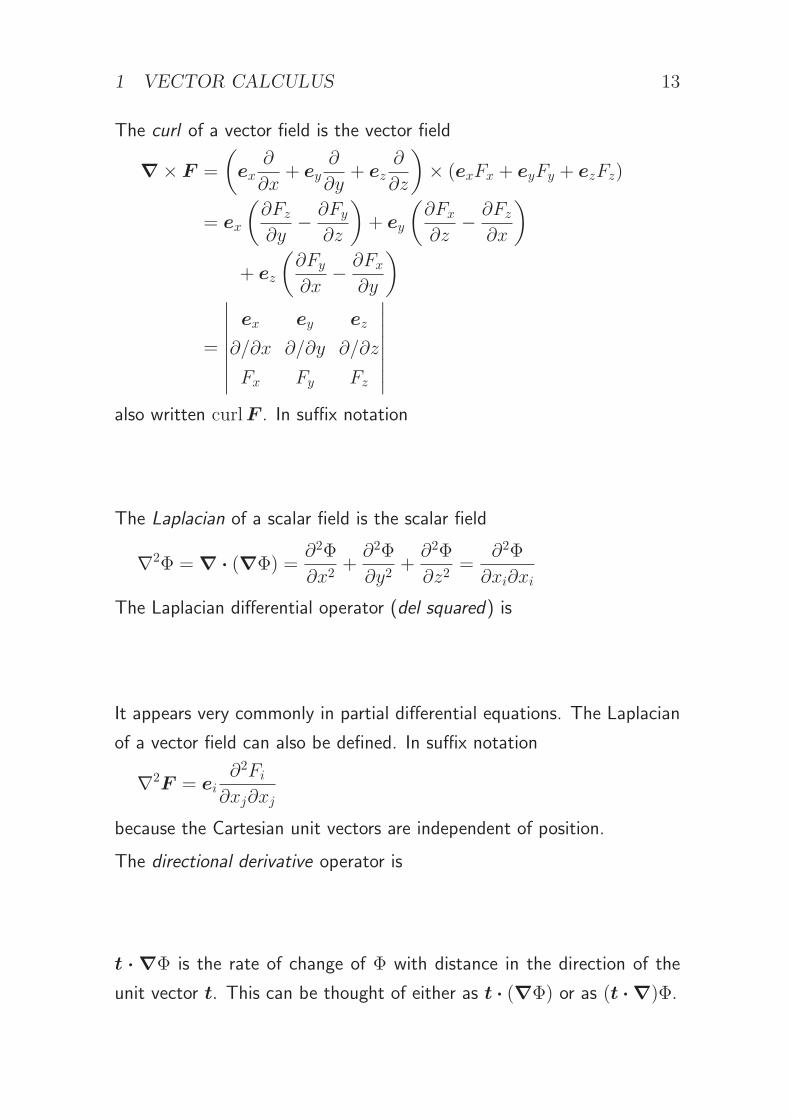
The curl of a vector field is the vector field
∇× F =
(
ex∂
∂x+ ey
∂
∂y+ ez
∂
∂z
)
× (exFx + eyFy + ezFz)
= ex
(
∂Fz
∂y−∂Fy
∂z
)
+ ey
(
∂Fx
∂z−∂Fz
∂x
)
+ ez
(
∂Fy
∂x−∂Fx
∂y
)
=
∣
∣
∣
∣
∣
∣
∣
∣
ex ey ez
∂/∂x ∂/∂y ∂/∂z
Fx Fy Fz
∣
∣
∣
∣
∣
∣
∣
∣
also written curlF . In suffix notation
∇× F = eiǫijk∂Fk
∂xjor (∇× F )i = ǫijk
∂Fk
∂xj
The Laplacian of a scalar field is the scalar field
∇2Φ = ∇ · (∇Φ) =∂2Φ
∂x2+∂2Φ
∂y2+∂2Φ
∂z2=
∂2Φ
∂xi∂xi
The Laplacian differential operator (del squared) is
∇2 =∂2
∂x2+
∂2
∂y2+
∂2
∂z2=
∂2
∂xi∂xi
It appears very commonly in partial differential equations. The Laplacian
of a vector field can also be defined. In suffix notation
∇2F = ei∂2Fi
∂xj∂xj
because the Cartesian unit vectors are independent of position.
The directional derivative operator is
t · ∇ = tx∂
∂x+ ty
∂
∂y+ tz
∂
∂z= ti
∂
∂xi
t · ∇Φ is the rate of change of Φ with distance in the direction of the
unit vector t. This can be thought of either as t · (∇Φ) or as (t · ∇)Φ.
1 VECTOR CALCULUS 14
Example . . . . . . . . . . . . . . . . . . . . . . . . . . . . . . . . . . . . . . . . . . . . . . . . . . . . . . . . . . . .
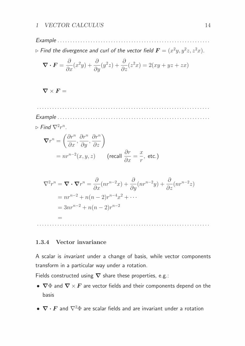
⊲ Find the divergence and curl of the vector field F = (x2y, y2z, z2x).
∇ · F =∂
∂x(x2y) +
∂
∂y(y2z) +
∂
∂z(z2x) = 2(xy + yz + zx)
∇× F =
∣
∣
∣
∣
∣
∣
∣
∣
ex ey ez
∂/∂x ∂/∂y ∂/∂z
x2y y2z z2x
∣
∣
∣
∣
∣
∣
∣
∣
= (−y2,−z2,−x2)
. . . . . . . . . . . . . . . . . . . . . . . . . . . . . . . . . . . . . . . . . . . . . . . . . . . . . . . . . . . . . . . . . . . .
Example . . . . . . . . . . . . . . . . . . . . . . . . . . . . . . . . . . . . . . . . . . . . . . . . . . . . . . . . . . . .
⊲ Find ∇2rn.
∇rn =
(
∂rn
∂x,∂rn
∂y,∂rn
∂z
)
= nrn−2(x, y, z) (recall∂r
∂x=x
r, etc.)
= nrn−2r
∇2rn = ∇ ·∇rn =∂
∂x(nrn−2x) +
∂
∂y(nrn−2y) +
∂
∂z(nrn−2z)
= nrn−2 + n(n− 2)rn−4x2 + · · ·
= 3nrn−2 + n(n− 2)rn−2
= n(n+ 1)rn−2
. . . . . . . . . . . . . . . . . . . . . . . . . . . . . . . . . . . . . . . . . . . . . . . . . . . . . . . . . . . . . . . . . . . .
1.3.4 Vector invariance
A scalar is invariant under a change of basis, while vector components
transform in a particular way under a rotation.
Fields constructed using ∇ share these properties, e.g.:
• ∇Φ and ∇×F are vector fields and their components depend on the
basis
• ∇ · F and ∇2Φ are scalar fields and are invariant under a rotation

1 VECTOR CALCULUS 15
grad, div and ∇2 can be defined in spaces of any dimension, but curl
(like the vector product) is a three-dimensional concept.
1.3.5 Vector differential identities
Here Φ and Ψ are arbitrary scalar fields, and F and G are arbitrary vector
fields.
Two operators, one field:
∇ · (∇Φ) = ∇2Φ
∇× (∇Φ) = 0
∇ · (∇× F ) = 0
∇× (∇× F ) = ∇(∇ · F )−∇2F
One operator, two fields:
∇(ΦΨ) = Ψ∇Φ + Φ∇Ψ
∇(F ·G) = (G · ∇)F +G× (∇× F ) + (F · ∇)G+ F × (∇×G)
∇ · (ΦF ) = (∇Φ) · F + Φ∇ · F
∇ · (F ×G) = G · (∇× F )− F · (∇×G)
∇× (ΦF ) = (∇Φ)× F + Φ∇× F
∇× (F ×G) = (G · ∇)F −G(∇ · F )− (F · ∇)G+ F (∇ ·G)
Example . . . . . . . . . . . . . . . . . . . . . . . . . . . . . . . . . . . . . . . . . . . . . . . . . . . . . . . . . . . .
⊲ Show that ∇ · (∇ × F ) = 0 for any (twice-differentiable) vector field
F .
∇ · (∇× F ) =∂
∂xi
(
ǫijk∂Fk
∂xj
)
= ǫijk∂2Fk
∂xi∂xj= 0
(since ǫijk is antisymmetric on (i, j) while ∂2Fk/∂xi∂xj is symmetric) .

1 VECTOR CALCULUS 16
Example . . . . . . . . . . . . . . . . . . . . . . . . . . . . . . . . . . . . . . . . . . . . . . . . . . . . . . . . . . . .
⊲ Show that∇×(F×G) = (G·∇)F−G(∇·F )−(F · ∇)G+F (∇·G).
∇× (F ×G) = eiǫijk∂
∂xj(ǫklmFlGm)
= eiǫkijǫklm∂
∂xj(FlGm)
= ei(δilδjm − δimδjl)
(
Gm
∂Fl
∂xj+ Fl
∂Gm
∂xj
)
= eiGj
∂Fi
∂xj− eiGi
∂Fj
∂xj+ eiFi
∂Gj
∂xj− eiFj
∂Gi
∂xj
= (G · ∇)F −G(∇ · F ) + F (∇ ·G)− (F · ∇)G
. . . . . . . . . . . . . . . . . . . . . . . . . . . . . . . . . . . . . . . . . . . . . . . . . . . . . . . . . . . . . . . . . . . .
Notes:
• be clear about which terms to the right an operator is acting on (use
brackets if necessary)
• you cannot simply apply standard vector identities to expressions in-
volving ∇, e.g. ∇ · (F ×G) 6= (∇× F ) ·G
• (G · ∇)F = Gj
∂
∂xjekFk
Related results:
• if a vector field F is irrotational (∇×F = 0) in a region of space, it
can be written as the gradient of a scalar potential : F = ∇Φ. e.g. a
‘conservative’ force field such as gravity
• if a vector field F is solenoidal (∇ · F = 0) in a region of space, it
can be written as the curl of a vector potential : F = ∇×G. e.g. the
magnetic field

1 VECTOR CALCULUS 17
1.4 Integral theorems
These very important results derive from the fundamental theorem of
calculus (integration is the inverse of differentiation):
∫ b
a
df
dxdx = f(b)− f(a)
1.4.1 The gradient theorem
∫
C
(∇Φ) · dr = Φ(r2)− Φ(r1)
where C is any curve from r1 to r2.
Outline proof:
∫
C
(∇Φ) · dr =
∫
C
dΦ
= Φ(r2)− Φ(r1)
1.4.2 The divergence theorem (Gauss’s theorem)
∫
V
(∇ · F ) dV =
∮
S
F · dS
where V is a volume bounded by the closed surface S (also called ∂V ).
The right-hand side is the flux of F through the surface S. The vector
surface element is dS = n dS, where n is the outward unit normal vector.
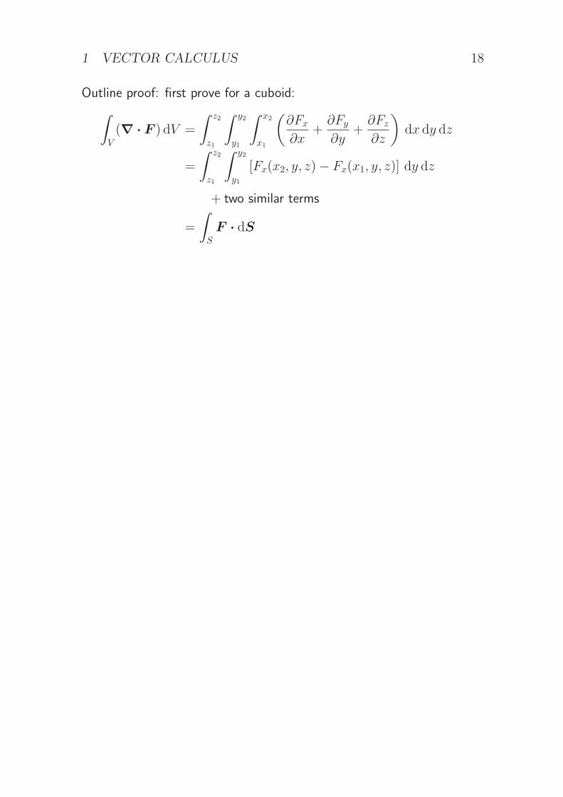
1 VECTOR CALCULUS 18
Outline proof: first prove for a cuboid:
∫
V
(∇ · F ) dV =
∫ z2
z1
∫ y2
y1
∫ x2
x1
(
∂Fx
∂x+∂Fy
∂y+∂Fz
∂z
)
dx dy dz
=
∫ z2
z1
∫ y2
y1
[Fx(x2, y, z)− Fx(x1, y, z)] dy dz
+ two similar terms
=
∫
S
F · dS

1 VECTOR CALCULUS 19
An arbitrary volume V can be subdivided into small cuboids to any desired
accuracy. When the integrals are added together, the fluxes through
internal surfaces cancel out, leaving only the flux through S.
A simply connected volume (e.g. a ball) is one with no holes. It has only
an outer surface. A multiply connected volume (e.g. a spherical shell)
may have more than one surface; all the surfaces must be considered.
1 VECTOR CALCULUS 20
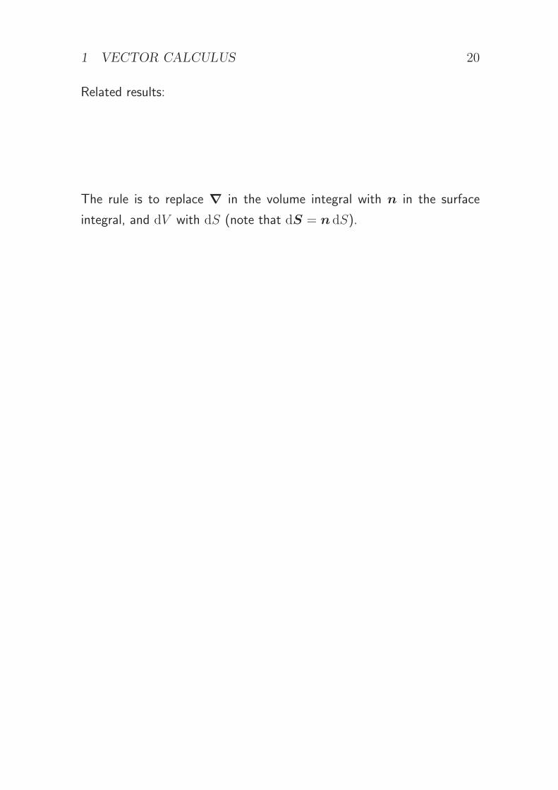
Related results:∫
V
(∇Φ) dV =
∮
S
ΦdS
∫
V
(∇× F ) dV =
∮
S
dS × F
The rule is to replace ∇ in the volume integral with n in the surface
integral, and dV with dS (note that dS = n dS).

1 VECTOR CALCULUS 21
Example . . . . . . . . . . . . . . . . . . . . . . . . . . . . . . . . . . . . . . . . . . . . . . . . . . . . . . . . . . . .
⊲ A submerged body is acted on by a hydrostatic pressure p = −ρgz,
where ρ is the density of the fluid, g is the gravitational acceleration and
z is the vertical coordinate. Find a simplified expression for the pressure
force acting on the body.
F = −
∮
S
p dS
Fz = ez · F =
∮
S
(−ezp) · dS
=
∫
V
∇ · (−ezp) dV
=
∫
V
∂
∂z(ρgz) dV
= ρg
∫
V
dV
=Mg (M is the mass of fluid displaced by the body)
Similarly
Fx =
∫
V
∂
∂x(ρgz) dV = 0
Fy = 0
F = ezMg
Archimedes’ principle: buoyancy force equals weight of displaced fluid
. . . . . . . . . . . . . . . . . . . . . . . . . . . . . . . . . . . . . . . . . . . . . . . . . . . . . . . . . . . . . . . . . . . .

1 VECTOR CALCULUS 22
1.4.3 The curl theorem (Stokes’s theorem)
∫
S
(∇× F ) · dS =
∮
C
F · dr
where S is an open surface bounded by the closed curve C (also called
∂S). The right-hand side is the circulation of F around the curve C.
Whichever way the unit normal n is defined on S, the line integral follows
the direction of a right-handed screw around n.
Special case: for a planar surface in the (x, y) plane, we have Green’s
theorem in the plane:
∫∫
A
(
∂Fy
∂x−∂Fx
∂y
)
dx dy =
∫
C
(Fx dx+ Fy dy)
where A is a region of the plane bounded by the curve C, and the line
integral follows a positive sense.

1 VECTOR CALCULUS 23
Outline proof: first prove Green’s theorem for a rectangle:
∫
A
(∇× F ) · dS =
∫ y2
y1
∫ x2
x1
(
∂Fy
∂x−∂Fx
∂y
)
dx dy
=
∫ y2
y1
[Fy(x2, y)− Fy(x1, y)] dy
−
∫ x2
x1
[Fx(x, y2)− Fx(x, y1)] dx
=
∫ x2
x1
Fx(x, y1) dx+
∫ y2
y1
Fy(x2, y) dy
+
∫ x1
x2
Fx(x, y2) dx+
∫ y1
y2
Fy(x1, y) dy
=
∫
C
(Fx dx+ Fy dy)
=
∮
C
F · dr
An arbitrary surface S can be subdivided into small planar rectangles
to any desired accuracy. When the integrals are added together, the
circulations along internal curve segments cancel out, leaving only the
circulation around C.
1 VECTOR CALCULUS 24
Notes:
• in Stokes’s theorem S is an open surface, while in Gauss’s theorem it
is closed
• many different surfaces are bounded by the same closed curve, while
only one volume is bounded by a closed surface
• a multiply connected surface (e.g. an annulus) may have more than
one bounding curve
1.4.4 Geometrical definitions of grad, div and curl
The integral theorems can be used to assign coordinate-independent mean-
ings to grad, div and curl.
Apply the gradient theorem to an arbitrarily small line segment δr = t δs
in the direction of any unit vector t. Since the variation of ∇Φ and t
along the line segment is negligible,
(∇Φ) · t δs ≈ δΦ
and so
t · (∇Φ) = limδs→0
δΦ
δs
This definition can be used to determine the component of ∇Φ in any
desired direction.
1 VECTOR CALCULUS 25
Similarly, by applying the divergence theorem to an arbitrarily small volume
δV bounded by a surface δS, we find that
∇ · F = limδV→0
1
δV
∫
δS
F · dS
Finally, by applying the curl theorem to an arbitrarily small open surface
δS with unit normal vector n and bounded by a curve δC, we find that
n · (∇× F ) = limδS→0
1
δS
∫
δC
F · dr
The gradient therefore describes the rate of change of a scalar field with
distance. The divergence describes the net source or efflux of a vector
field per unit volume. The curl describes the circulation or rotation of a
vector field per unit area.
1.5 Orthogonal curvilinear coordinates
Cartesian coordinates can be replaced with any independent set of co-
ordinates q1(x1, x2, x3), q2(x1, x2, x3), q3(x1, x2, x3), e.g. cylindrical or
spherical polar coordinates.
Curvilinear (as opposed to rectilinear) means that the coordinate ‘axes’ are
curves. Curvilinear coordinates are useful for solving problems in curved
geometry (e.g. geophysics).
1.5.1 Line element
The infinitesimal line element in Cartesian coordinates is
dr = ex dx+ ey dy + ez dz
In general curvilinear coordinates we have
dr = h1 dq1 + h2 dq2 + h3 dq3
1 VECTOR CALCULUS 26
where
hi = eihi =∂r
∂qi(no sum)
determines the displacement associated with an increment of the coordi-
nate qi.
hi = |hi| is the scale factor (or metric coefficient) associated with the
coordinate qi. It converts a coordinate increment into a length. Any point
at which hi = 0 is a coordinate singularity at which the coordinate system
breaks down.
ei is the corresponding unit vector. This notation generalizes the use of
ei for a Cartesian unit vector. For Cartesian coordinates, hi = 1 and ei
are constant, but in general both hi and ei depend on position.
The Einstein summation convention does not work well with orthogonal
curvilinear coordinates.
1.5.2 The Jacobian
The Jacobian of (x, y, z) with respect to (q1, q2, q3) is defined as
J =∂(x, y, z)
∂(q1, q2, q3)=
∣
∣
∣
∣
∣
∣
∣
∣
∂x/∂q1 ∂x/∂q2 ∂x/∂q3
∂y/∂q1 ∂y/∂q2 ∂y/∂q3
∂z/∂q1 ∂z/∂q2 ∂z/∂q3
∣
∣
∣
∣
∣
∣
∣
∣
This is the determinant of the Jacobian matrix of the transformation from
coordinates (x1, x2, x3) to (q1, q2, q3). The columns of the above matrix
are the vectors hi defined above. Therefore the Jacobian is equal to the
scalar triple product
J = [h1,h2,h3] = h1 · h2 × h3
Given a point with curvilinear coordinates (q1, q2, q3), consider three small
displacements δr1 = h1 δq1, δr2 = h2 δq2 and δr3 = h3 δq3 along the

1 VECTOR CALCULUS 27
three coordinate directions. They span a parallelepiped of volume
δV = |[δr1, δr2, δr3]| = |J | δq1 δq2 δq3
Hence the volume element in a general curvilinear coordinate system is
dV =
∣
∣
∣
∣
∂(x, y, z)
∂(q1, q2, q3)
∣
∣
∣
∣
dq1 dq2 dq3
The Jacobian therefore appears whenever changing variables in a multiple
integral:∫
Φ(r) dV =
∫∫∫
Φdx dy dz =
∫∫∫
Φ
∣
∣
∣
∣
∂(x, y, z)
∂(q1, q2, q3)
∣
∣
∣
∣
dq1 dq2 dq3
The limits on the integrals also need to be considered. Note that if
|J | = 0 anywhere in the range of variables, the coordinate transformation
is invalid.
Jacobians are defined similarly for transformations in any number of di-
mensions. If curvilinear coordinates (q1, q2) are introduced in the (x, y)-
plane, the area element is
dA = |J | dq1 dq2
with
J =∂(x, y)
∂(q1, q2)=
∣
∣
∣
∣
∣
∂x/∂q1 ∂x/∂q2
∂y/∂q1 ∂y/∂q2
∣
∣
∣
∣
∣
The equivalent rule for a one-dimensional integral is∫
f(x) dx =
∫
f(x(q))
∣
∣
∣
∣
dx
dq
∣
∣
∣
∣
dq
The modulus sign appears here if the integrals are carried out over a
positive range (the upper limits are greater than the lower limits).

1 VECTOR CALCULUS 28
1.5.3 Properties of Jacobians
Consider now three sets of variables αi, βi and γi, with 1 6 i 6 n, none
of which need be Cartesian coordinates. According to the chain rule of
partial differentiation,
∂αi
∂γj=
n∑
k=1
∂αi
∂βk
∂βk∂γj
(Under the summation convention we may omit the Σ sign.) The left-hand
side is the ij-component of the Jacobian matrix of the transformation
from αi to γi. The equation states that this matrix is the product of the
Jacobian matrices of the transformations from αi to βi and from βi to γi.
Taking the determinant of this matrix equation, we find
∂(α1, · · · , αn)
∂(γ1, · · · , γn)=∂(α1, · · · , αn)
∂(β1, · · · , βn)
∂(β1, · · · , βn)
∂(γ1, · · · , γn)
This is the chain rule for Jacobians: the Jacobian matrix of a composite
transformation is the product of the Jacobian matrices of the transforma-
tions of which it is composed.
In the special case in which γi = αi for all i, the left-hand side is 1 (the
determinant of the unit matrix) and we obtain
∂(α1, · · · , αn)
∂(β1, · · · , βn)=
[
∂(β1, · · · , βn)
∂(α1, · · · , αn)
]−1
The Jacobian of an inverse transformation is therefore the reciprocal of
that of the forward transformation. This is a multidimensional general-
ization of the result dx/dy = (dy/dx)−1.
1.5.4 Orthogonality of coordinates
Calculus in general curvilinear coordinates is difficult. We can make things
easier by choosing the coordinates to be orthogonal:
ei · ej = δij

1 VECTOR CALCULUS 29
and right-handed:
e1 × e2 = e3
The squared line element is then
|dr|2 = |e1 h1 dq1 + e2 h2 dq2 + e3 h3 dq3|2
= h21dq2
1+ h2
2dq2
2+ h2
3dq2
3
There are no cross terms such as dq1 dq2.
When oriented along the coordinate directions:
• line element dr = e1 h1 dq1
• surface element dS = e3 h1h2 dq1 dq2,
• volume element dV = h1h2h3 dq1 dq2 dq3
Note that, for orthogonal coordinates, J = h1 · h2 × h3 = h1h2h3

1 VECTOR CALCULUS 30
1.5.5 Commonly used orthogonal coordinate systems
Cartesian coordinates (x, y, z):
−∞ < x <∞, −∞ < y <∞, −∞ < z <∞
r = (x, y, z)
hx =∂r
∂x= (1, 0, 0)
hy =∂r
∂y= (0, 1, 0)
hz =∂r
∂z= (0, 0, 1)
hx = 1, ex = (1, 0, 0)
hy = 1, ey = (0, 1, 0)
hz = 1, ez = (0, 0, 1)
r = x ex + y ey + z ez
dV = dx dy dz
Orthogonal. No singularities.

1 VECTOR CALCULUS 31
Cylindrical polar coordinates (ρ, φ, z):
0 < ρ <∞, 0 6 φ < 2π, −∞ < z <∞
r = (x, y, z) = (ρ cosφ, ρ sinφ, z)
hρ =∂r
∂ρ= (cosφ, sinφ, 0)
hφ =∂r
∂φ= (−ρ sinφ, ρ cosφ, 0)
hz =∂r
∂z= (0, 0, 1)
hρ = 1, eρ = (cosφ, sinφ, 0)
hφ = ρ, eφ = (− sinφ, cosφ, 0)
hz = 1, ez = (0, 0, 1)
r = ρ eρ + z ez
dV = ρ dρ dφ dz
Orthogonal. Singular on the axis ρ = 0.
Warning 1. Many authors use r for ρ and θ for φ. This is confusing
because r and θ then have different meanings in cylindrical and spher-
ical polar coordinates. Instead of ρ, which is useful for other things,
some authors use R, s or .

1 VECTOR CALCULUS 32
Spherical polar coordinates (r, θ, φ):
0 < r <∞, 0 < θ < π, 0 6 φ < 2π
r = (x, y, z) = (r sin θ cosφ, r sin θ sinφ, r cos θ)
hr =∂r
∂r= (sin θ cosφ, sin θ sinφ, cos θ)
hθ =∂r
∂θ= (r cos θ cosφ, r cos θ sinφ,−r sin θ)
hφ =∂r
∂φ= (−r sin θ sinφ, r sin θ cosφ, 0)
hr = 1, er = (sin θ cosφ, sin θ sinφ, cos θ)
hθ = r, eθ = (cos θ cosφ, cos θ sinφ,− sin θ)
hφ = r sin θ, eφ = (− sinφ, cosφ, 0)
r = r er
dV = r2 sin θ dr dθ dφ
Orthogonal. Singular on the axis r = 0, θ = 0 and θ = π.
Notes:
• cylindrical and spherical are related by ρ = r sin θ, z = r cos θ
• plane polar coordinates are the restriction of cylindrical coordinates to
a plane z = constant
1 VECTOR CALCULUS 33
1.5.6 Vector calculus in orthogonal coordinates
A scalar field Φ(r) can be regarded as function of (q1, q2, q3):
dΦ =∂Φ
∂q1dq1 +
∂Φ
∂q2dq2 +
∂Φ
∂q3dq3
=
(
e1
h1
∂Φ
∂q1+
e2
h2
∂Φ
∂q2+
e3
h3
∂Φ
∂q3
)
· (e1 h1 dq1 + e2 h2 dq2 + e3 h3 dq3)
= (∇Φ) · dr
We identify
∇Φ =e1
h1
∂Φ
∂q1+
e2
h2
∂Φ
∂q2+
e3
h3
∂Φ
∂q3
Thus
∇qi =ei
hi(no sum)
We now consider a vector field in orthogonal coordinates:
F = e1F1 + e2F2 + e3F3
Finding the divergence and curl are non-trivial because both Fi and ei
depend on position. First, consider
∇× (q2∇q3) = (∇q2)× (∇q3) =e2
h2×
e3
h3=
e1
h2h3
which implies
∇ ·
(
e1
h2h3
)
= 0
as well as cyclic permutations of this result. Second, we have
∇×
(
e1
h1
)
= ∇× (∇q1) = 0, etc.
1 VECTOR CALCULUS 34
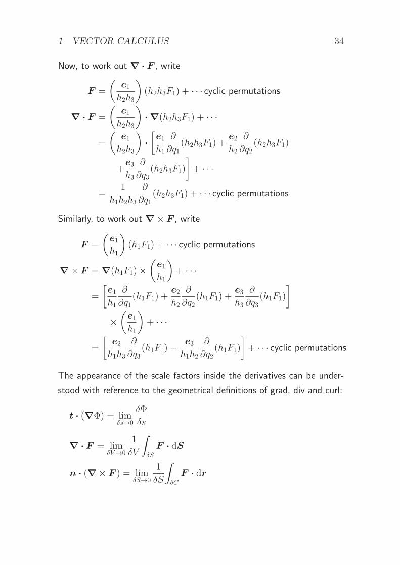
Now, to work out ∇ · F , write
F =
(
e1
h2h3
)
(h2h3F1) + · · · cyclic permutations
∇ · F =
(
e1
h2h3
)
· ∇(h2h3F1) + · · ·
=
(
e1
h2h3
)
·
[
e1
h1
∂
∂q1(h2h3F1) +
e2
h2
∂
∂q2(h2h3F1)
+e3
h3
∂
∂q3(h2h3F1)
]
+ · · ·
=1
h1h2h3
∂
∂q1(h2h3F1) + · · · cyclic permutations
Similarly, to work out ∇× F , write
F =
(
e1
h1
)
(h1F1) + · · · cyclic permutations
∇× F = ∇(h1F1)×
(
e1
h1
)
+ · · ·
=
[
e1
h1
∂
∂q1(h1F1) +
e2
h2
∂
∂q2(h1F1) +
e3
h3
∂
∂q3(h1F1)
]
×
(
e1
h1
)
+ · · ·
=
[
e2
h1h3
∂
∂q3(h1F1)−
e3
h1h2
∂
∂q2(h1F1)
]
+ · · · cyclic permutations
The appearance of the scale factors inside the derivatives can be under-
stood with reference to the geometrical definitions of grad, div and curl:
t · (∇Φ) = limδs→0
δΦ
δs
∇ · F = limδV→0
1
δV
∫
δS
F · dS
n · (∇× F ) = limδS→0
1
δS
∫
δC
F · dr
1 VECTOR CALCULUS 35
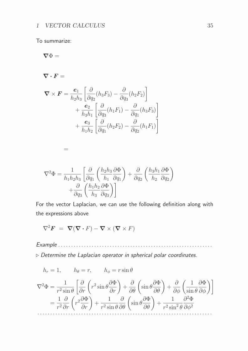
To summarize:
∇Φ =e1
h1
∂Φ
∂q1+
e2
h2
∂Φ
∂q2+
e3
h3
∂Φ
∂q3
∇ · F =1
h1h2h3
[
∂
∂q1(h2h3F1) +
∂
∂q2(h3h1F2) +
∂
∂q3(h1h2F3)
]
∇× F =e1
h2h3
[
∂
∂q2(h3F3)−
∂
∂q3(h2F2)
]
+e2
h3h1
[
∂
∂q3(h1F1)−
∂
∂q1(h3F3)
]
+e3
h1h2
[
∂
∂q1(h2F2)−
∂
∂q2(h1F1)
]
=1
h1h2h3
∣
∣
∣
∣
∣
∣
∣
∣
h1 e1 h2 e2 h3 e3
∂/∂q1 ∂/∂q2 ∂/∂q3
h1F1 h2F2 h3F3
∣
∣
∣
∣
∣
∣
∣
∣
∇2Φ =1
h1h2h3
[
∂
∂q1
(
h2h3h1
∂Φ
∂q1
)
+∂
∂q2
(
h3h1h2
∂Φ
∂q2
)
+∂
∂q3
(
h1h2h3
∂Φ
∂q3
)]
For the vector Laplacian, we can use the following definition along with
the expressions above
∇2F = ∇(∇ · F )−∇× (∇× F )
Example . . . . . . . . . . . . . . . . . . . . . . . . . . . . . . . . . . . . . . . . . . . . . . . . . . . . . . . . . . . .
⊲ Determine the Laplacian operator in spherical polar coordinates.
hr = 1, hθ = r, hφ = r sin θ
∇2Φ =1
r2 sin θ
[
∂
∂r
(
r2 sin θ∂Φ
∂r
)
+∂
∂θ
(
sin θ∂Φ
∂θ
)
+∂
∂φ
(
1
sin θ
∂Φ
∂φ
)]
=1
r2∂
∂r
(
r2∂Φ
∂r
)
+1
r2 sin θ
∂
∂θ
(
sin θ∂Φ
∂θ
)
+1
r2 sin2 θ
∂2Φ
∂φ2. . . . . . . . . . . . . . . . . . . . . . . . . . . . . . . . . . . . . . . . . . . . . . . . . . . . . . . . . . . . . . . . . . . .

1 VECTOR CALCULUS 36
1.5.7 Grad, div, curl and ∇2 in cylindrical and spherical
polar coordinates
Cylindrical polar coordinates:
∇Φ = eρ∂Φ
∂ρ+
eφ
ρ
∂Φ
∂φ+ ez
∂Φ
∂z
∇ · F =1
ρ
∂
∂ρ(ρFρ) +
1
ρ
∂Fφ
∂φ+∂Fz
∂z
∇× F =1
ρ
∣
∣
∣
∣
∣
∣
∣
∣
eρ ρ eφ ez
∂/∂ρ ∂/∂φ ∂/∂z
Fρ ρFφ Fz
∣
∣
∣
∣
∣
∣
∣
∣
∇2Φ =1
ρ
∂
∂ρ
(
ρ∂Φ
∂ρ
)
+1
ρ2∂2Φ
∂φ2+∂2Φ
∂z2
Spherical polar coordinates:
∇Φ = er∂Φ
∂r+
eθ
r
∂Φ
∂θ+
eφ
r sin θ
∂Φ
∂φ
∇ · F =1
r2∂
∂r(r2Fr) +
1
r sin θ
∂
∂θ(sin θ Fθ) +
1
r sin θ
∂Fφ
∂φ
∇× F =1
r2 sin θ
∣
∣
∣
∣
∣
∣
∣
∣
er r eθ r sin θ eφ
∂/∂r ∂/∂θ ∂/∂φ
Fr rFθ r sin θ Fφ
∣
∣
∣
∣
∣
∣
∣
∣
∇2Φ =1
r2∂
∂r
(
r2∂Φ
∂r
)
+1
r2 sin θ
∂
∂θ
(
sin θ∂Φ
∂θ
)
+1
r2 sin2 θ
∂2Φ
∂φ2
1 VECTOR CALCULUS 37
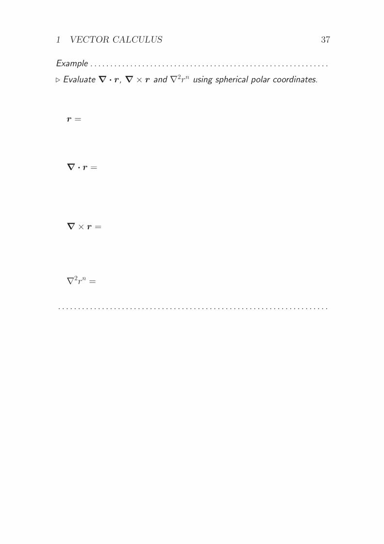
Example . . . . . . . . . . . . . . . . . . . . . . . . . . . . . . . . . . . . . . . . . . . . . . . . . . . . . . . . . . . .
⊲ Evaluate ∇ · r, ∇× r and ∇2rn using spherical polar coordinates.
r = err
∇ · r =1
r2∂
∂r(r2 · r) = 3
∇× r =1
r2 sin θ
∣
∣
∣
∣
∣
∣
∣
∣
er r eθ r sin θ eφ
∂/∂r ∂/∂θ ∂/∂φ
r 0 0
∣
∣
∣
∣
∣
∣
∣
∣
= 0
∇2rn =1
r2∂
∂r
(
r2∂rn
∂r
)
= n(n+ 1)rn−2
. . . . . . . . . . . . . . . . . . . . . . . . . . . . . . . . . . . . . . . . . . . . . . . . . . . . . . . . . . . . . . . . . . . .
2 PARTIAL DIFFERENTIAL EQUATIONS 38
2 Partial differential equations
2.1 Motivation
The variation in space and time of scientific quantities is usually described
by differential equations. If the quantities depend on space and time, or
on more than one spatial coordinate, then the governing equations are
partial differential equations (PDEs).
Many of the most important PDEs are linear and classical methods of
analysis can be applied. The techniques developed for linear equations
are also useful in the study of nonlinear PDEs.
2.2 Linear PDEs of second order
2.2.1 Definition
We consider an unknown function u(x, y) (the dependent variable) of
two independent variables x and y. A partial differential equation is any
equation of the form
F
(
u,∂u
∂x,∂u
∂y,∂2u
∂x2,∂2u
∂x∂y,∂2u
∂y2, . . . , x, y
)
= 0
involving u and any of its derivatives evaluated at the same point.
• the order of the equation is the highest order of derivative that appears
• the equation is linear if F depends linearly on u and its derivatives
A linear PDE of second order has the general form
Lu = f
where L is a differential operator such that
Lu = a∂2u
∂x2+ b
∂2u
∂x∂y+ c
∂2u
∂y2+ d
∂u
∂x+ e
∂u
∂y+ gu

2 PARTIAL DIFFERENTIAL EQUATIONS 39
where a, b, c, d, e, f, g are functions of x and y.
• if f = 0 the equation is said to be homogeneous
• if a, b, c, d, e, g are independent of x and y the equation is said to have
constant coefficients
These ideas can be generalized to more than two independent variables,
or to systems of PDEs with more than one dependent variable.
2.2.2 Principle of superposition
L defined above is an example of a linear operator :
L(αu) = αLu
and
L(u+ v) = Lu+ Lv
where u and v any functions of x and y, and α is any constant.
The principle of superposition:
• if u and v satisfy the homogeneous equation Lu = 0, then αu and
u+ v also satisfy the homogeneous equation
• similarly, any linear combination of solutions of the homogeneous equa-
tion is also a solution
• if the particular integral up satisfies the inhomogeneous equation Lu =
f and the complementary function uc satisfies the homogeneous equa-
tion Lu = 0, then up + uc also satisfies the inhomogeneous equation:
L(up + uc) = Lup + Luc = f + 0 = f
The same principle applies to any other type of linear equation (e.g. al-
gebraic, ordinary differential, integral).
2 PARTIAL DIFFERENTIAL EQUATIONS 40
2.2.3 Classic examples
Laplace’s equation:
∇2u = 0
Diffusion equation (heat equation):
∂u
∂t= λ∇2u, λ = diffusion coefficient (or diffusivity)
Wave equation:
∂2u
∂t2= c2∇2u, c = wave speed
All involve the vector-invariant operator ∇2, the form of which depends
on the number of active dimensions.
Inhomogeneous versions of these equations are also found. The inhomo-
geneous term usually represents a ‘source’ or ‘force’ that generates or
drives the quantity u.
2.3 Physical examples of occurrence
2.3.1 Examples of Laplace’s (or Poisson’s) equation
Gravitational acceleration is related to gravitational potential by
g = −∇Φ
The source (divergence) of the gravitational field is mass:
∇ · g = −4πGρ
where G is Newton’s constant and ρ is the mass density. Combine:
∇2Φ = 4πGρ
2 PARTIAL DIFFERENTIAL EQUATIONS 41
External to the mass distribution, we have Laplace’s equation ∇2Φ = 0.
With the source term the inhomogeneous equation is called Poisson’s
equation.
Analogously, in electrostatics, the electric field is related to the electro-
static potential by
E = −∇Φ
The source of the electric field is electric charge:
∇ ·E =ρ
ǫ0
where ρ is the charge density and ǫ0 is the permittivity of free space.
Combine to obtain Poisson’s equation:
∇2Φ = −ρ
ǫ0
The vector field (g or E) is said to be generated by the potential Φ. A
scalar potential is easier to work with because it does not have multiple
components and its value is independent of the coordinate system. The
potential is also directly related to the energy of the system.
2.3.2 Examples of the diffusion equation
A conserved quantity with density (amount per unit volume) Q and flux
density (flux per unit area) F satisfies the conservation equation:
∂Q
∂t+∇ · F = 0
This is more easily understood when integrated over the volume V bounded
by any (fixed) surface S:
d
dt
∫
V
Q dV =
∫
V
∂Q
∂tdV = −
∫
V
∇ · F dV = −
∫
S
F · dS
2 PARTIAL DIFFERENTIAL EQUATIONS 42
The amount of Q in the volume V changes only as the result of a net
flux through S.
Often the flux of Q is directed down the gradient of Q through the linear
relation (Fick’s law)
F = −λ∇Q
Combine to obtain the diffusion equation (if λ is independent of r):
∂Q
∂t= λ∇2Q
In a steady state Q satisfies Laplace’s equation.

2 PARTIAL DIFFERENTIAL EQUATIONS 43
Example . . . . . . . . . . . . . . . . . . . . . . . . . . . . . . . . . . . . . . . . . . . . . . . . . . . . . . . . . . . .
⊲ Heat conduction in a solid. Conserved quantity: energy. Heat per unit
volume: CT (C is heat capacity per unit volume, T is temperature. Heat
flux density: −K∇T (K is thermal conductivity). Thus
∂
∂t(CT ) +∇ · (−K∇T ) = 0
or
∂T
∂t= λ∇2T, λ =
K
C
e.g. copper: λ ≈ 1 cm2 s−1 . . . . . . . . . . . . . . . . . . . . . . . . . . . . . . . . . . . . . . . . . .
Further example: concentration of a contaminant in a gas. λ ≈ 0.2 cm2 s−1
2 PARTIAL DIFFERENTIAL EQUATIONS 44
2.3.3 Examples of the wave equation
Waves on a string. The string has uniform mass per unit length ρ
and uniform tension T . The transverse displacement y(x, t) is small
(|∂y/∂x| ≪ 1) and satisfies Newton’s second law for an element δs of
the string:
(ρ δs)∂2y
∂t2= δFy ≈
∂Fy
∂xδx
Now,
Fy = T sin θ ≈ T tan θ ≈ T∂y
∂x, and also δs ≈ δx
where θ is the small angle between the x-axis and the tangent to the
string. Combine to obtain the one-dimensional wave equation
∂2y
∂t2= c2
∂2y
∂x2, c =
√
T
ρ
e.g. violin (D-)string: T ≈ 40N, ρ ≈ 1 gm−1: c ≈ 200ms−1
Electromagnetic waves. Maxwell’s equations for the electromagnetic field
in a vacuum:
∇ ·E = 0
∇ ·B = 0
∇×E +∂B
∂t= 0
1
µ0∇×B − ǫ0
∂E
∂t= 0

2 PARTIAL DIFFERENTIAL EQUATIONS 45
where E is electric field, B is magnetic field, µ0 is the permeability of
free space and ǫ0 is the permittivity of free space. Eliminate E:
∂2B
∂t2= −∇×
∂E
∂t= −
1
µ0ǫ0∇× (∇×B)
Now use the identity ∇× (∇×B) = ∇(∇ ·B)−∇2B and Maxwell’s
equation ∇ ·B = 0 to obtain the (vector) wave equation
∂2B
∂t2= c2∇2B, c =
√
1
µ0ǫ0
E obeys the same equation. c is the speed of light. c ≈ 3× 10⁸ms−1
Further example: sound waves in a gas. c ≈ 300ms−1
2.3.4 Examples of other second-order linear PDEs
Schrodinger’s equation (quantum-mechanical wavefunction of a particle
of mass m in a potential V ):
i~∂ψ
∂t= −
~2
2m∇2ψ + V (r)ψ
Helmholtz equation (arises in wave problems):
∇2u+ k2u = 0
Klein–Gordon equation (arises in relativistic quantum mechanics):
∂2u
∂t2= c2(∇2u−m2u)
2.3.5 Examples of nonlinear PDEs
Burgers’ equation (describes shock waves):
∂u
∂t+ u
∂u
∂x= λ∇2u
2 PARTIAL DIFFERENTIAL EQUATIONS 46
Nonlinear Schrodinger equation (describes solitons, e.g. in optical fibre
communication):
i∂ψ
∂t= −∇2ψ − |ψ|2ψ
These equations require different methods of analysis.
2.4 Separation of variables (Cartesian coordinates)
2.4.1 Diffusion equation
We consider the one-dimensional diffusion equation (e.g. conduction of
heat along a metal bar):
∂u
∂t= λ
∂2u
∂x2
The bar could be considered finite (having two ends), semi-infinite (having
one end) or infinite (having no end). Typical boundary conditions at an
end are:
• u is specified (Dirichlet boundary condition)
• ∂u/∂x is specified (Neumann boundary condition)
If a boundary is removed to infinity, we usually require instead that u be
bounded (i.e. remain finite) as x → ±∞. This condition is needed to
eliminate unphysical solutions.
To determine the solution fully we also require initial conditions. For the
diffusion equation this means specifying u as a function of x at some
initial time (usually t = 0).
Try a solution in which the variables appear in separate factors:
u(x, t) = X(x)T (t)
Substitute this into the PDE:
X(x)T ′(t) = λX ′′(x)T (t)
2 PARTIAL DIFFERENTIAL EQUATIONS 47
(recall that a prime denotes differentiation of a function with respect to
its argument). Divide through by λXT to separate the variables:
T ′(t)
λT (t)=X ′′(x)
X(x)
The LHS depends only on t, while the RHS depends only on x. Both
must therefore equal a constant, which we call −k2 (for later convenience
here – at this stage the constant could still be positive or negative). The
PDE is separated into two ordinary differential equations (ODEs)
T ′ + λk2T = 0
X ′′ + k2X = 0
with general solutions
T = A exp(−λk2t)
X = B sin(kx) + C cos(kx)
Finite bar : suppose the Neumann boundary conditions ∂u/∂x = 0 (i.e.
zero heat flux) apply at the two ends x = 0, L. Then the admissible
solutions of the X equation are
X = C cos(kx), k =nπ
L, n = 0, 1, 2, . . .
These boundary conditions rule out solutions with negative k2. Combine
the factors to obtain the elementary solution (let C = 1 WLOG)
u = A cos(nπx
L
)
exp
(
−n2π2λt
L2
)
Each elementary solution represents a ‘decay mode’ of the bar. The
decay rate is proportional to n2. The n = 0 mode represents a uniform
temperature distribution and does not decay.
2 PARTIAL DIFFERENTIAL EQUATIONS 48
The principle of superposition allows us to construct a general solution as
a linear combination of elementary solutions:
u(x, t) =∞∑
n=0
An cos(nπx
L
)
exp
(
−n2π2λt
L2
)
The coefficients An can be determined from the initial conditions. If the
temperature at time t = 0 is specified, then
u(x, 0) =∞∑
n=0
An cos(nπx
L
)
is known. The coefficients An are just the Fourier coefficients of the initial
temperature distribution.
Semi-infinite bar : The solution X ∝ cos(kx) is valid for any real value
of k so that u is bounded as x → ∞. We may assume k > 0 WLOG.
The solution decays in time unless k = 0. The general solution is a linear
combination in the form of an integral:
u =
∫ ∞
0
A(k) cos(kx) exp(−λk2t) dk
This is an example of a Fourier integral, studied in section 4.
Notes:
• separation of variables doesn’t work for all linear equations, by any
means, but it does for some of the most important examples
• it is not supposed to be obvious that the most general solution can be
written as a linear combination of separated solutions
2.4.2 Wave equation (example)
∂2u
∂t2= c2
∂2u
∂x2, 0 < x < L
Boundary conditions:
u = 0 at x = 0, L

2 PARTIAL DIFFERENTIAL EQUATIONS 49
Initial conditions:
u,∂u
∂tspecified at t = 0
Trial solution:
u(x, t) = X(x)T (t)
X(x)T ′′(t) = c2X ′′(x)T (t)
T ′′(t)
c2T (t)=X ′′(x)
X(x)= −k2 b.c. dictate k2 > 0
T ′′ + c2k2T = 0
X ′′ + k2X = 0
T = A sin(ckt) + B cos(ckt)
X = C sin(kx), k =nπ
L, n = 1, 2, 3, . . .
Elementary solution:
u =
[
A sin
(
nπct
L
)
+B cos
(
nπct
L
)]
sin(nπx
L
)
General solution:
u =∞∑
n=1
[
An sin
(
nπct
L
)
+Bn cos
(
nπct
L
)]
sin(nπx
L
)
At t = 0:
u =∞∑
n=1
Bn sin(nπx
L
)
∂u
∂t=
∞∑
n=1
(nπc
L
)
An sin(nπx
L
)
The Fourier series for the initial conditions determine all the coefficients
An, Bn.

2 PARTIAL DIFFERENTIAL EQUATIONS 50
2.4.3 Helmholtz equation (example)
A three-dimensional example in a cube:
∇2u+ k2u = 0, 0 < x, y, z < L
Boundary conditions:
u = 0 on the boundaries
Trial solution:
u(x, y, z) = X(x)Y (y)Z(z)
X ′′(x)Y (y)Z(z) +X(x)Y ′′(y)Z(z) +X(x)Y (y)Z ′′(z)
+ k2X(x)Y (y)Z(z) = 0
X ′′(x)
X(x)+Y ′′(y)
Y (y)+Z ′′(z)
Z(z)+ k2 = 0
The variables are separated: each term must equal a constant. Call the
constants −k2x,−k2
y,−k2
z , since exponentials, the solutions with positive
constants, cannot satisfy the boundary conditions:
X ′′ + k2xX = 0
Y ′′ + k2yY = 0
Z ′′ + k2zZ = 0
k2 = k2x + k2y + k2z
X ∝ sin(kxx), kx =nxπ
L, nx = 1, 2, 3, . . .
Y ∝ sin(kyy), ky =nyπ
L, ny = 1, 2, 3, . . .
Z ∝ sin(kzz), kz =nzπ
L, nz = 1, 2, 3, . . .

2 PARTIAL DIFFERENTIAL EQUATIONS 51
Elementary solution:
u = A sin(nxπx
L
)
sin(nyπy
L
)
sin(nzπz
L
)
The solution is possible only if k2 is one of the discrete values
k2 = (n2x + n2y + n2z)π2
L2
These are the eigenvalues of the problem.