NATIONAL BUREAU OF ECONOMIC RESEARCH IMPLICATIONS …

NBER WORKING PAPER SERIES

A MODEL OF INTERNATIONAL CITIES:IMPLICATIONS FOR REAL EXCHANGE RATES

Mario J. CruciniHakan Yilmazkuday

Working Paper 14834http://www.nber.org/papers/w14834

NATIONAL BUREAU OF ECONOMIC RESEARCH1050 Massachusetts Avenue

Cambridge, MA 02138April 2009

We especially thank Mary Amiti, Eric Bond, Paolo Pesenti and Robert Vigfusson for valuable commentsand criticisms. We grateful to seminar participants at the California State University -- Long Beach,Federal Reserve Banks of Dallas and New York, Utah State University, Temple University, Universityof Tennessee at Knoxville and Vanderbilt University; conference participants at the 2008 MidwestInternational Economics Meeting at The Ohio State University, the 2008 Midwest Annual Meetingparticipants in Chicago, IL, the Wegman's Conference at the University of Rochester, and the MurrayS. Johnson Memorial Conference, The University of Texas at Austin. The authors gratefully acknowledgethe financial support of the National Science Foundation (SES-0136979, SES-0524868). The viewsexpressed herein are those of the author(s) and do not necessarily reflect the views of the NationalBureau of Economic Research.

NBER working papers are circulated for discussion and comment purposes. They have not been peer-reviewed or been subject to the review by the NBER Board of Directors that accompanies officialNBER publications.

© 2009 by Mario J. Crucini and Hakan Yilmazkuday. All rights reserved. Short sections of text, notto exceed two paragraphs, may be quoted without explicit permission provided that full credit, including© notice, is given to the source.

A Model of International Cities: Implications for Real Exchange RatesMario J. Crucini and Hakan YilmazkudayNBER Working Paper No. 14834April 2009JEL No. F0,F15

ABSTRACT

We develop a model of cities each inhabited by two agents, one specializing in manufacturing, theother in distribution. The distribution sector represents the physical transformation of all internationallytraded goods from the factory gate to the final consumer. Using a panel of micro-prices at the citylevel, we decompose the long-run variance of LOP deviations into the fraction due to distribution costs,trade costs and a residual. For the median good, trade costs account for 50 percent of the variance,distribution costs account for 10 percent with 40 percent of the variance unexplained. Since the sampleof items in the data are heavily skewed toward traded goods, we also decompose the variance basedon the median good on an expenditure-weighted basis. Now the tables turn, with distribution costsaccounting for 43 percent, trade costs 36 percent and 21 percent of the variance unexplained.

Mario J. CruciniDepartment of EconomicsVanderbilt UniversityBox 1819 Station BNashville, TN 37235-1819and [email protected]

Hakan YilmazkudayDepartment of EconomicsVanderbilt UniversityBox 1819 Station BNashville, TN [email protected]

1. Introduction

According to the U.S. National Income and Product Accounts, expenditure by consumers at

the retail level is about twice what producers receive for the same goods and services. This

di¤erence has come to be called the distribution margin. The distribution margin includes

transportation costs from the factory gate to the �nal point of consumption as well costs

and markups at the wholesale and retail stage.

Most existing international models abstract from the distribution sector entirely and focus

on the fraction of transportation costs attributable to international shipments. Abstracting

from the distribution sector is problematic for three reasons. First, the distribution sector

may help us to understand the large and persistent deviations from the Law-of-One-Price

(LOP) and Purchasing Power Parity. Second, the general equilibrium interaction of the

distribution sector and the production sector is not well understood. Given the prominent

role of the dichotomy between traded and non-traded goods in international �nance, this is

an important omission. Recent evidence also suggests that information technology and scale

economies in distribution have altered the e¢ ciency and markup structure of the distribution

sector (e.g., the Walmart e¤ect). These developments may have fundamentally altered price

dispersion and dynamics, both across locations within countries and across countries. Third,

the distribution sector includes the �nancial, legal, medical and education sectors. These

sectors have grown immensely in economic importance over time. Much of the economic

activity engaged by these sectors is geographically segmented due either to the arms-length

nature of the exchange, public policy decisions or some combination of the two. Since the

shares of expenditure attributable to these sectors tend to rise with the level of development,

their economic importance continues to rise globally.

We have two related goals in this paper. The �rst is to develop a tractable stochastic

general equilibrium model of production and distribution at the microeconomic level of

individual goods and services across cities. The second is to use the theory to specify a

regression model to estimate microeconomic parameters of a cost function, speci�c to an

individual retail good or service, which includes the cost of distribution as well as the more

traditional inputs of capital and labor embodied in traded inputs. This cost function is used

3

to conduct a variance decomposition of prices across cities into a distribution margin, a trade

cost margin and a residual, good-by-good. The distribution margin is further parsed into the

in�uences of labor and retail infrastructure costs across cities. The Economist Intelligence

Unit (EIU) retail price data along with supplementary sources for wages at the city level

are used in the empirical work. Since the model assumes perfect competition and abstracts

from o¢ cial barriers to trade, the residual in the regression equation is expected to include

markups, o¢ cial barriers to trade and measurement error.

In the model, each city is inhabited by two representative agents, a manufacturer and

a retailer. The manufacturer produces a single homogeneous good using labor as the only

input. The manufactured good is shipped to all other cities of the world and deviations

in the prices of these traded goods re�ect only shipping costs from the factory door to the

receiving dock at the retail establishment. The retailer transforms these goods by combining

them with her labor and a �xed factor; she may also produce pure services which require no

traded inputs at all. The �xed factor is intended to capture retail infrastructure, broadly

de�ned to include land, buildings, equipment and public infrastructure.

The advantage of drilling down to the level of individual goods and services at the city

level is that we can learn a great deal about production structure from the cross-sectional

variance in the data. What distinguishes the manufacturing sector from the distribution

sector is intimately related to what distinguishes a personal computer from a haircut. Ag-

gregating the data tends to obscure these di¤erences. For example, if trade costs are

symmetric, aggregating across imports and exports has the e¤ect of understating their role.

Having cities as the locations allows both greater attention to the spatial dimensions of man-

ufacturing specialization and a more precise measure of the distance between production and

consumption locations.

We have two sets of results, one for the sources of LOP variance for the median good,

the other for the di¤erences in the sources of variance across goods in the cross-section.

For the median good in the EIU sample, trade costs account for about 50 percent of LOP

deviations, the distribution margin accounts for about 10 percent and the remaining 40

percent is unaccounted for. Because the median good in the EIU has a distribution share

of only 0.2, well below the aggregate value of 0.5 in the U.S. National Income and Product

4

Accounts, we also report results centered on this value. Now the tables turn, with distribution

costs accounting for 43 percent, trade costs 36 percent percent and 21 percent of the variance

unexplained.

The relative importance of trade and distribution is fairly stable across sets of locations

that include high and low income countries and when comparing within country and cross-

border city pairs. The absolute level of cross-sectional variance rises when a border is crossed

as one would expect or when comparisons are made between cities with vastly di¤erent wealth

levels. One exception is the division of the variance accounted for by the distribution sector

into the cost of labor and capital. Variance across low income countries is dominated by

di¤erences in the capital component, with labor playing a small role. For other countries,

the division of the distribution margin across labor and capital is closer to equality.

Turning to di¤erences in geographic price dispersion across goods, we �nd substantial

heterogeneity consistent with Crucini, Telmer and Zachariadis (2005) who focused on Eu-

ropean Union capital cities using Eurostat micro-price data. The structure of the model

and methodology allow us to say more about the underlying sources of this heterogeneity.

In the international data, the distribution margin accounts for 50 percent of cross-sectional

variance in LOP deviations for the good with the highest distribution share and this fraction

falls to a mere 10 percent as we move to the good with the lowest distribution share. Retail

infrastructure accounts for more than 30 percent of the cross-sectional variance in LOP de-

viations across Canada and the United States for the good with the highest infrastructure

intensity, while accounting for virtually none of the variance for the good with the lowest

infrastructure intensity.

Our theoretical model is closest to Giri (2009) who adds a good-speci�c distribution

cost to the Eaton-Kortum (2002) model. In Giri�s model distribution services are in �xed

proportion to the physical units of the base good as in Burstein, Neves and Rebelo (2003)

(BNR) with e¢ ciencies drawn from a distribution with a country-speci�c mean and common

world-wide variance. In contrast, we assume that the technological parameter for distribution

inputs is good�speci�c while the productivity of the distribution sector is city-speci�c. Given

that this margin is measurable in the NIPA, we view this as a more tractable way to model the

distribution sector than the random e¢ ciency approach. Our model shares with Alvarez and

5

Lucas (2007), Atkeson and Burstein (2007), Eaton and Kortum (2002), and Kanda Naknoi

(2008) an interest in the role of traditional trade costs. However, to the extent these papers

incorporate a distribution sector, it is a common wedge across all goods in the retail basket,

which assumes away any cross-sectional variance in price deviations due to the distribution

margin. We �nd this heterogeneity to be essential for improving our understanding of LOP

deviations.

2. The Model

Each city, indexed by j, is inhabited by two representative agents. As is usual in representa-

tive agent frameworks, these two agents should be viewed as stand-ins for a large number of

atomistic agents of each type, since we will be assuming perfect competition in all factor and

�nal goods markets throughout. One agent specializes in the production of a single traded

good, indexed by i, while the other specializes in retail trade and production of non-traded

services. Production in the manufacturing sector is proportional to labor input, the factor

of proportionality is a random productivity variable. Retail production requires both labor

and capital. Capital is �xed and is broadly de�ned to include land, buildings, equipment

and public infrastructure. Productivity varies across cities in both the traded goods sector

and the retail sector.

Traded goods are subject to iceberg transportation costs which are good and destination

speci�c. Final goods and local inputs (retailer labor and retail capital) are not traded beyond

the city limits. While hours and consumption are both choice variables, the assumptions we

make in the model imply constant hours in all sectors in all locations, reminiscent of the

Long and Plosser (1983) multi-sector, closed economy, real business cycle model. Retail

infrastructure, including land, capital and equipment, is in �xed supply (denoted Kj).

The good index, i, distinguishes physical objects from the identities of agents and loca-

tions only when needed to avoid confusion. In describing the �ow of goods from one location

to another, the source is the �rst subscript and the destination is the second subscript. Thus,

Xsd refers to the shipment of good X, from city s to city d. Given the assumption that in-

dividuals at each location specialize, s also indexes the good and the individual to whom

6

the income �ows, while d indicates the expenditure side of the equation. � sd is the iceberg

shipping cost from the source to the destination. Since there are no durable goods or assets

in the model, adding time subscripts is innocuous: they are omitted here since the focus is

on the steady-state properties of the model and long-run deviations from the LOP.

The full solution for quantities and prices is given in the appendix. This section presents

the complete model and parts of the equilibrium solution relevant for pricing implications,

which is the focus of our empirical work.

2.1. Consumers

Agents preferences are log-additive over consumption and leisure:

U�CAj ; L

Aj

�� (1� �) logCAj + � logLAj , A = m; s. (2.1)

CAj is aggregate consumption and LAj is hours of leisure, for an individual working in city

j. There are two individuals in each city, indexed by A = m; s; one is engaged in the

manufacture of a single good (m) and the other is engaged in retailing and service activities

(s).

The consumption aggregate is CES over varieties of manufactured goods produced world-

wide:

CAj =

MXi

(�i)1"�CAij� "�1

"

! ""�1

. (2.2)

CAij is the consumption of good i in city j by worker of type A; " > 0 is the elasticity of

substitution across goods, �i is a good speci�c taste parameter and M is the number of

manufactured goods in existence. M is also the number of cities given our specialization

assumption.

The two agents inhabiting city j, maximize utility (2.1) subject to their respective budget

constraints: Xi

PijCAij � WA

j NAj + '

AHjKj (2.3)

where Pij is the price of good i in destination city j. These prices will be the same for all

agents in the same location, but di¤er across locations for reasons described below. Each of

the two residents of city j earn labor income from their production activities and split the

7

rental income accruing to the retail infrastructure in their city ('m + 's = 1), the stock of

which is assumed to be �xed at Kj. The rental price of retail infrastructure is denoted Hj.

The consumer�s problem may be solved in two stages. In the �rst stage, the consumer

chooses aggregate consumption and leisure, subject to a budget and time allocation con-

straint. In the second stage, the consumer minimizes expenditure across goods. Here we

collapse the problem to a single stage for brevity. The key equations from the solution to

the consumer�s problem are:

CAij = �i

�PijPj

��"CAj (2.4)

CAj =WAj N

Aj + '

AHjKj

Pj(2.5)

NAj = 1� � � 'A�HjKj

WAj

(2.6)

LAj = � + 'A�HjKj

WAj

(2.7)

Aggregate real consumption is nominal consumption de�ated by the ideal de�ator Pj ��Pi �i (Pij)

1�"� 11�" , which ensures

Pi PijCij = PjCj as well as a theoretical mapping from

price indices to welfare.

The �rst equation determines consumption demand for a particular good as a function

of the relative price of the good paid by the �nal consumer in their home market and that

individual�s aggregate consumption level. It is important to note that, Pij is the retail price

of good i, in city j; it embodies the cost of local retail services paid to the retailer in addition

to the traditional iceberg trade costs of the imported item. The price index, is a weighted

average of these retail prices, the closest empirical counterpart would be the CPI index. The

second equation is aggregate consumption of an agent, which is equal to her real income.

Real income is the sum of nominal wage and rental income, de�ated by the local price level,

Pj.

The last two equations determine hours of work and leisure. In the absence of rental

income, the two agents would work the same number of hours, independent of their relative

wage, due to the o¤setting income and substitution e¤ect of wages on e¤ort with Cobb-

Douglas preferences. In the presence of rental income the requirement for constant e¤ort

in equilibrium is that the ratio of rental income to labor income be constant. Most growth

8

models impose restrictions on tastes and technology to ensure constancy of hours per capita

in the presence of trending productivity.1

2.2. Manufacturers

The production function for manufactured good, i, is:

Yi = AiNmi (2.8)

where Ai is the productivity level and Nmi is hours of work.

Manufacturers choose labor inputs to maximize pro�ts:

maxNmi

(QiiYi �Wmi N

mi ) . (2.9)

The manufacturer receives the factor gate price, Qii, for every unit produced, no matter where

the goods end up being sold. Given the assumptions of constant returns to scale, perfect

competition and one factor of production, the factory gate price equals the manufacturing

wage divided by productivity:

Qii =Wmi

Ai. (2.10)

Given specialization, the productivity level in this expression is good and city-speci�c. The

presence of a nation-speci�c component could easily be incorporated by allowing Ai to have

a common factor across cities located within the same country.

Retailers in each city purchase the manufactured goods and pay a proportional shipping

cost. Thus the retail purchase price is the factory-gate price marked up by a proportional

shipping cost:

Qij = (1 + � ij)Qii = (1 + � ij)Wmi =Ai (2.11)

where � ij > 0 is the net transportation cost from city i to j. Qij is the price the retailer pays

in the destination city. The empirical counterpart to this would be a wholesale price. The

local manufacturing plant is close enough to the city to ignore local transportation costs so

that � ii = 0. E¤ectively this cuts out one intermediary, the wholesaler, and the retailer is

1Details of these restrictions in the context of the one sector stochastic growth model may be found in

King, Plosser and Rebelo (1988).

9

viewed as operating next to the factor gate. The destination price of the manufactured good

depends: i) positively on both the manufacturing wage and the trade cost; and ii) negatively

on manufacturing productivity.

2.3. Retailers

The retailer in each city optimally chooses how much of each manufactured good to purchase

from various cities of the world. The retailer transforms these goods using a fraction of her

time endowment and some amount of the local retail infrastructure. The retailer then sells

the resulting composite good in the local retail market. The production function for good i,

sold in city j is:

Rij =��BjN

sij

� i (Kij)1� i

�1��i(Gij)

�i (2.12)

Gij is the amount of the manufactured good imported from city i, by a retailer in city

j. N sij is the fraction of the retailer�s time endowment allocated to the transformation of

imported good i for local consumption in city j and Kij is the amount of retail infrastructure

allocated to retail good i in city j. Bj is labor-augmenting productivity speci�c to the city

(equivalently, the retailer), common to all goods sold there.2

While the production function is restricted to be common to all locations, it is very

�exible across goods. It captures pure labor services (e.g., baby-sitting services) with �i

equal to zero and i equal to one; internet purchases (e.g., Amazon.com book purchases), �i

equal to one, and all points in between.

The retailer in city, j, maximizes pro�ts from the sale of each good, i, by optimally

choosing the three inputs needed to produce the good: i) the amount of the traded input,

Gij, to import ii) the fraction of her time to devote to the good, N sij; and iii) how much local

infrastructure to allocate to the activity, Kij:

maxNsij ;Kij ;Gij

(PijRij �W sjN

sij �HjKij �QijGij) (2.13)

At the optimum, the unit price equals marginal cost. Given constant returns to scale and

three factors of production, the retail price of good i sold in location j, is a Cobb-Douglas

2In principle one could add good-speci�c productivity of retailers to account for di¤erent levels of com-

petency across goods, but we lack productivity data to operationalize this idea.

10

aggregate of the price (inclusive of trade cost) that the retailer paid to acquire the traded

input, Qij, the retailer�s market wage, W sj , and the rental price of retail infrastructure, Hj:

Pij = MCsij = �i

��W sj =Bj

� i (Hj)(1� i)�(1��i) (Qij)�i (2.14)

��1i � ��ii

�(1� �i) ( i)

i (1� i)(1� i)

�(1��i)(2.15)

The retail price in city j is rising in input prices and falling in retail productivity, Bj.

2.4. Equilibrium

The appendix contains the tedious algebra necessary to arrive at the equilibrium allocations

discussed in this section. In the remainder of the paper the consumption aggregator is

restricted to Cobb-Douglas to arrive at closed form solutions.

In the global general equilibrium, all the optimality conditions of partial equilibrium must

hold for consumers, retailers and manufacturers. In addition, the supply of each good must

equal its total demand, including the resources lost to iceberg shipping costs.

Yi =Xj

Gij(1 + � ij) (2.16)

=Xj

Gij +Xj

Gij� ij (2.17)

= Gi + Ti (2.18)

In words: the production of good i, Yi, is exhausted between the global demand for that

good by retailers aggregated across destinations, Gi, and physical loses due to iceberg costs,

Ti.

Each individual has a �xed amount of time to devote to hours of work and leisure, here,

normalized to unity. The time constraints for the manufacturers and the retailers are thus:

Lmj +Nmj = 1 (2.19)

Lsj +Xi

N sij = 1 . (2.20)

The summation in the second time constraint re�ects the fact that the retailer must divide

her time across theM di¤erent retailing activities. The notation implicitly sets the number

of goods at the retail level equal to the number of goods in the manufacturing sector. Nothing

11

we derive requires this: we could have some activities that use no traded inputs at all in

which case the number of retail goods would exceed the number of manufacturing goods by

the number of pure services produced by �retailers�in each city.

The city�s retail infrastructure is exhausted across uses:

Kj =Xi

Kij .

3. The data

Our focus is retail price dispersion across international cities at the microeconomic and

macroeconomic level. The data source for prices is the Economist Intelligence Unit (EIU)

worldwide retail price survey. The survey spans 123 cities, located in 79 countries. Most of

the cities are national capitals. The larger number of cities than countries is due to the fact

that the survey also includes multiple cities in a few countries. Noteworthy are the 16 U.S.

cities included in the survey; the next largest number of cities surveyed equals 5 in Australia,

China and Germany. Up to data availability for particular years and cities, the number of

goods and services priced is 301. The available sample is 1990 to 2005.

Our goal is to understand the sources of variation in LOP deviations. The Cobb-Douglas

functional forms in our model rationalize the use of logarithms of LOP deviations across

bilateral city-pairs:

qijk;t = ln(Sjk;tPij;t=Pik;t) . (3.1)

while our long-run focus further suggests the use of time-averaged deviations:

qijk = T�1X

tqijk;t . (3.2)

Crucini and Telmer (2007) derive a variance decomposition which is very useful for splitting

the total variance of LOP deviations into long-run deviations and time series �uctuations:

V arjk;t(qi;jk;t j i) = V arjk(Et[qi;jk;t j i; jk]) + Ejk[V art(qi;jk;t j i; jk)] (3.3)

Vi = Ti + Fi : (3.4)

The �rst term, Ti, which is meant to remind the reader of trade costs broadly de�ned, is

the focus of this paper. It is the variance of the deviations from the LOP across all location

12

pairs remaining after time-averages of the data have been taken. The role of time-averaging

is to eliminate the time series component of the variation, which is valid when the data

are stationary and su¢ ciently long time samples are available, which is the case here. The

second term, Fi, which is to remind the reader of �uctuations, is the focus of the international

�nance literature, often featuring short-run �uctuations of LOP due to local currency price

stickiness. One of the novel �ndings of Crucini and Telmer is that the ratio of the variance

of the long-run deviations to the total (i.e., Ti=Vi) is very large for the average good: 0.51

for U.S.-Canada intranational pairs and 0.69 for all international city pairs in the EIU data.

In other words, the variance component this model focuses upon is at least as important in

an accounting sense as the focus of business cycle models.

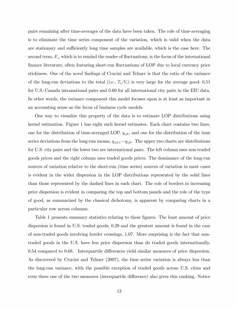
One way to visualize this property of the data is to estimate LOP distributions using

kernel estimation. Figure 1 has eight such kernel estimates. Each chart contains two lines,

one for the distribution of time-averaged LOP, qijk, and one for the distribution of the time

series deviations from the long-run means, qijk;t�qijk. The upper two charts are distributions

for U.S. city pairs and the lower two are international pairs. The left column uses non-traded

goods prices and the right column uses traded goods prices. The dominance of the long-run

sources of variation relative to the short-run (time series) sources of variation in most cases

is evident in the wider dispersion in the LOP distributions represented by the solid lines

than those represented by the dashed lines in each chart. The role of borders in increasing

price dispersion is evident in comparing the top and bottom panels and the role of the type

of good, as summarized by the classical dichotomy, is apparent by comparing charts in a

particular row across columns.

Table 1 presents summary statistics relating to these �gures. The least amount of price

dispersion is found in U.S. traded goods, 0.29 and the greatest amount is found in the case

of non-traded goods involving border crossings, 1.07. More surprising is the fact that non-

traded goods in the U.S. have less price dispersion than do traded goods internationally,

0.54 compared to 0.68. Interquartile di¤erences yield similar measures of price dispersion.

As discovered by Crucini and Telmer (2007), the time series variation is always less than

the long-run variance, with the possible exception of traded goods across U.S. cities and

even there one of the two measures (interquartile di¤erence) also gives this ranking. Notice

13

also that the distinction between traded and non-traded goods is obvious in the long-run

measure, but ambiguous in the time series measure. Given our emphasis on trade costs,

broadly de�ned and abstraction from stochastic variation due to shocks interacting with

sticky prices, this observation is another reason to focus on the time averaged data with our

model.

The EIU survey o¤ers little in the way of wage data. Supplemental wage data at the

country level come from the International Labor Organization (ILO) survey of occupational

and sectoral wages and at the city level from the Union Bank of Switzerland (UBS) survey.

The ILO data are averages for countries. They span 49 sectors, 162 occupations and 137

countries. The sample period is annual from 1983 to 2003. The complete list of these sectors,

occupations, and countries is found in Oostendorp (2003). In the raw ILO data, the most

common period is the month, followed by the hour, but some countries report weekly pay,

others give daily rates for some occupations, and so on. In order to have a comparable wage

data across countries, the standardized version of ILO survey by Oostendorp (2003) is used:

in cases in which the wage data are reported as hourly or daily, then these wages were made

(roughly) comparable with monthly wages by multiplication by 160 and 20 respectively. In

order to have the largest panel of wage data that are comparable across countries, the monthly

wages in US dollars that have been obtained by country-speci�c and uniform calibration in

Oostendorp (2003) are used.

Wage data at the city level is more appropriate given the EIU retail price data is city

based and the intent of the model. International cities were surveyed by the UBS in 2006.

These are hourly wages in US dollars, spanning occupations in 71 international cities, 60

of which are also surveyed by the EIU. Among the 60 EIU cities there are four cities from

Brazil, Canada, China, France, Italy, Spain and Switzerland; four cities from Germany, and

four cities from the U.S. The hourly wages have been obtained by dividing the income per

year in each occupation by the city level hours of work in a year, where the latter we collected

by a survey, also conducted by the UBS.

Bureau of Labor Statistics (BLS) city wage data from the Occupational Employment

Statistics (OES) Survey in 2006 are used to complement UBS data. These wage data are

hourly wages in US dollars for the same 16 US cities found in EIU retail price survey.

14

The combination of UBS and BLS wage data, then, provides wage data for 72 EIU cities,

comprised of 16 from the BLS and the remainder (non-U.S. cities) from the UBS. Within

these 72 EIU cities, in terms of intranational cities, we have two cities from Brazil, Canada,

China, France, Italy, Spain and Switzerland; three cities from Germany, and 16 cities from

the US.3

In a preliminary part of the analysis, the BLS city wage data are used for broader wage

dispersion analysis. These data cover two industries, namely production and sales, for 400

cities (on average) within the U.S. in terms of hourly wages from 1999 to 2006.

A number of trade-o¤s present themselves in terms of the model focus and the available

data. Country-level wage data is generally available for longer periods of time, but fewer

locations than city-level wage data. Since the model is explicitly constructed to mimic city

level aggregation and steady-state features, ideally one would want long time series at the

city level. Unfortunately these are simply not available. These trade-o¤s are discussed as

they arise below.

Land prices and rents are even more di¢ cult to come by than are wages and prices. We

use the EIU survey data item: �Typical annual gross rent for top-quality units, 2,000 square

meters, suitable for warehousing or factory use.�4

The other two pieces of information are sectoral estimates of the distribution shares, 1��,

which are calculated from a combination of U.S. NIPA data and input-output tables. The

NIPA data extend to 57 sectors, while the input-output data span 33 sectors. The NIPA

shares are computed as the value the producers receive relative to the value consumers pay

for the output of a particular sector. The distribution margin, 1��, includes transportation

costs, retail and distribution costs and markups. Sectors involving arms-length transactions,

such as medical services are recorded in the NIPA as though the producer and consumer

valuation is equal. While this is literally true in some cases, this accounting fails to distinguish

3In an earlier version of this paper we used PWT per capita annual income data covering the annual

period from 1990 to 2004 to proxy for real wages. These data span all 79 EIU countries. The results were

qualitatively similar to those reported here.4One additional commerical rental price is available in the EIU, �Typical annual gross rent for a 1,000

square meter unit in a Class A building in a prime location.�Results are very similar with this alternative

measure.

15

local inputs from traded inputs used in the production of services. For these sectors we use

the input-output tables to determine the distribution share. These sectoral measures from

the NIPA complement the good-level parameters estimated using a regression framework

discussed below.

Finally, the greater circle distance between cities in the EIU sample is used to estimate

the trade cost component of the LOP deviations at the retail level.5

4. Microeconomic sources of long-run variation in wages

In the model, wage deviations arise across the retail and manufacturing sectors and across

cities. The amount of labor income accruing to the manufacturer relative to the retailer in

city j is,Nmj W

mj

N sjW

sj

=

Pi �i�iP

i (1� �i) i�i(4.1)

Which is intuitive: the numerator is an expenditure share weighted average of labor�s share

of manufacturing and the denominator is the counterpart in retailing. The appearance of

the parameter i in the denominator accounts for the fact that retail production involves

some retail infrastructure, unless i = 1, in which case retail production is labor-only. Note,

also, that the ratio is the same in all cities.

As the primary interest is wage variation across cities as an explanation for cost and

price variation across cities, we would like to understand the wage ratio and e¤ort ratios

separately. The equilibrium relative sectoral wage is given by:

Wmj

W sj

='m

1� 'm(1� �)�N s

j

(1� �)�Nmj

Thus, given �xed shares of rental income across agents in the city, relative wages and relative

hours move inversely as one would expect. The appendix shows that the equilibrium e¤ort

5Hummels (2001) provides the most comprehensive estimates of sectoral trade costs using import unit

values, a more direct method than employed here. Unfortunately these estimates are available for a limited

number of countries and are more aggregated than our retail data.

16

levels are:

Nmj =

(1� �0) (1� �)(1� �0) + 'm� (�0 � �1)

N sj =

�1 (1� �)�1 + '

s� (�0 � �1)

where �0 �P

i (1� �i) �i and �1 �P

i (1� �i) i�i. E¤ort in both sectors is declining in

the share of rental income allocated to the agent (a wealth e¤ect), and in the preference for

leisure (�), as one would expect.

Substituting these expressions into the wage ratio leads to the following expression for

relative wages:Wmj

W sj

=1� 'm'm

(1� �0) + 'A��1 + (1� 'A)�

� = � (�0 � �1).

As the retail sector becomes more labor intensive (thus reducing rental income), (�0 � �1)

converges to zero and the model reverts to the labor-only version with a common fraction of

available hours worked by both agents, equal to (1� �) and the sectoral wage ratio converges

to:Wmj

W sj

=1� �0�0

=

Pi �i�iP

i (1� �i) �iwhich is exactly the same expression as labor income shares in the more general case (see

equation (4.1)).

Turning to wage di¤erences across cities things are much simpler even in the general

case:

W sj

W sk

=�j�j�k�k

(4.2)

Wmj

Wmk

=�j�j�k�k

. (4.3)

The cross-city wage di¤erential is the same in both sectors and is determined by the product

of the taste and technology parameters in the two locations being compared. The intuition

for this result is as follows. Consider, �rst, the special case in which all goods use traded

inputs in the same proportion, �j = �. Wages are higher in locations that produce the

17

goods most preferred by consumers, given by the comparison of �j and �k, a demand-side

e¤ect. Next, consider the case with symmetric tastes across goods �j = �; then wages are

the highest for producers of manufactures requiring the least amount of input from retailers

(i.e., the lowest 1� �). Essentially, the higher the distribution share, the less productive is

an hour allocated to production of the manufactured good in terms of delivering a unit of

consumption to �nal consumers. This lowers the equilibrium real wage.

Wage data are available by occupation or sector of employment. Our model focuses on

the distinction between goods and services, suggesting the production sector de�nition is

more appropriate. However, we use both labor classi�cations as a robustness check.

The more comprehensive of the sources used is the ILO survey of wage levels across

countries. These data span 49 sectors, 162 occupations and 137 countries. The sample

period is annual from 1983 to 2003.6 Because the model is intended to be based on city-level

data, the preferred measure is wage data from the UBS that span 14 occupations and 71

international cities for the year 2006.

According to the model, if the retail sector uses only labor and traded goods, the ratio

of manufacturing wages to service wages provides on estimate of the overall scale of the

distribution sectorWmj =W

sj = �=1��, � =

Pi �i�i. Since we lack consumption expenditure

shares at the present time, we associate this with the distribution share alone since using the

symmetric taste version of the model we have: � = �. A direct way to measure the overall

size of the distribution sector is to use U.S. NIPA data and input-output data. Crucini and

Shintani (2008) do exactly this and �nd � = 0:57. The advantage of their calculation is that

is it based on expenditure weighting of sectoral ��s.

Table 2 reports the sectoral wage ratio averaged across locations as well as the implied

value for �. It turns out that the direct and indirect (model-based) estimates are equal when

U.S. wages in production sector relative to the sales sector are used. The wage ratio in the

international data is consistent with a value � of 0.52. While this is a modest di¤erence from

the U.S. value, the implied manufacturing wage premium is quite dramatically a¤ected: it

is a factor of 5 smaller than the U.S. case. It could be that relative productivity di¤erences

are the cause. Another possibility is that the U.S. and international agencies have di¤erent

6Useful technical documentation is found in Remco H. Oostendorp (2003).

18

classi�cation systems for the sectors.

As the theory is a two-sector model, any sectoral variation in wages in a particular city

is attributable to wage di¤erences across the manufacturing and service sectors. Variation

in wages across sub-sectors are abstracted from entirely. Thus, it is important for the theory

that wages di¤er signi�cantly across locations and less so across sectors other than the two

sectors emphasized by the model (retail and manufacturing). And this is what is found.

Table 3 conducts a variance decomposition by sector and country for time-averaged wages

in the case of the ILO survey and an analogous decomposition by sector and city for wages

in 2006 for the UBS survey data. Since the answer may depend on the set of sectors and

locations used, we consider three location groups and allow for many sectors throughout.

The location groups are the entire world, the OECD and the LDC.

Based on the ILO wage data: locations account for between 72 and 85 percent of the

cross-sectional variation in wages, sectoral di¤erences account for less than 10 percent. The

dominance of location in accounting for wage dispersion is somewhat less pronounced when

the data is organized by occupation: location e¤ects drop to between 38 and 65 percent.

Most of di¤erence is not attributed to a pure sectoral component, but rather an interaction

of location and sector. The UBS tell a similar story to the ILO for location e¤ects, with the

occupation e¤ect rising in contribution due to a lower interaction with location compared to

the ILO.

In sum, location is a key component of wage dispersion with the precise fractions depend-

ing somewhat on the set of locations examined and the precise de�nition of wage categories.

5. Microeconomic sources of long-run variation in real exchange

rates

We turn, now, to the main focus, price dispersion. In the model, prices consumers actually

pay may di¤er from factory gate prices for two reasons. The �rst is the trade cost to import

the good from the foreign production location. The second is the value added by the retailer.

To simplify the notation, all international prices have been converted to common currency

units (it does not matter which numeraire is chosen). The ratio of the price of good i in city

19

j relative to k, based on the theory is:

PijPik

=

�W sj =Bj

W sk=Bk

� i(1��i)�HjHk

�(1� i)(1��i)�QijQik

��i.

Noting that the last term reduces to the ratio of trade costs from the single source of good i

to each of the destinations, j and k and taking logs, de�nes the Law-of-One-Price deviation

across a city pair:

qijk = (1� �i) [ i!jk + (1� i)hjk] + �i� ijk (5.1)

= �i!jk + �ihjk + �i� ijk .

The retail margin is the �rst term in square braces; it is a weighted average of the productivity-

adjusted wage and the rental price di¤erential faced by retailers in the two cities. The weights

attached to the relative input prices in the retail sector depend on i. The entire retail com-

ponent gets weighted by its overall share in the production of the �nal good, (1� �i). The

second term is the relative trade cost. The last line, used to specify our regression approach,

expresses the relationship in terms of the three key cost ratios, retail wages, rental prices

and trade costs.

The aggregate real exchange rate in our theory follows directly from equation (5.1) since

the consumption aggregator is Cobb-Douglas (i.e., " = 1):

qjk = �!jk + �hjk +X

i�i�i� ijk (5.2)

� �X

i�i i(1� �i), � �

Xi�i(1� i)(1� �i)

The aggregate real exchange rate has a number of interesting features. The distribution

component of the PPP deviations are driven by exactly the same wage and rental price dif-

ferentials as was true of the LOP deviations, the impact factors are consumption-expenditure-

weighted production parameters, � and �. The trade cost component is more convoluted

because the expenditure shares, production coe¢ cients, and trade costs are good speci�c.

However, it seems plausible that the individual deviations could average out across goods

since the � ijk are expected to vary in sign across goods.

20

5.1. Regression speci�cation

This section conducts a variance decomposition of retail prices into the channels described

by the equilibrium model. Adding a measurement error term to the theoretical equation for

the LOP deviation, gives:

qijk = �i!jk + �ihjk + �i� ijk + "ijk (5.3)

Data on retail prices, wages and rent, are available, but no data on retail productivity or

trade costs exist for this cross-section of locations, at this level of disaggregation. The raw

wage ratios are used in place of !jk and a two-stage estimation approach is used to infer the

impact of trade costs.

The �rst-stage regression is:

qijk = �1i!jk + �1ihjk + �ijk. (5.4)

where �ijk is an estimated residual, which, according to the theory, is the LOP deviation in

the traded component of cost. In practice it will incorporate other sources of deviations

as well. In an attempt to purge these other factors from the pure trade cost component,

the estimated residuals are projected on bilateral distances. To accomplish this, de�ne the

direction-of-trade indicator function:

Iijk =

8<: 1 if �ijk > 0

�1 if �ijk < 0(5.5)

where �ijk = qijk��1i!jk��1ihjk from the �rst-stage regression. In words: imports (exports)

are assumed to be relatively expensive (inexpensive) at the destination (source).

Consider, now, the more elaborate equation for stage two:

qijk = �2i!jk + �2ihjk + & i2Iijkdjk + "ijk (5.6)

�2i = (1� �i) i (5.7)

�2i = (1� �i)(1� i) (5.8)

&2i = �i�i (5.9)

with the trade cost replaced by Iijk�idjk. The indicator function ensures the sign of the

implied trade cost is consistent with the sign of the residual estimated in stage one. The

21

greatest circle distance between locations j and k is the empirical counterpart to djk and

goods are allowed to have di¤erent trade cost elasticities with respect to distance, �i. The

bene�t of projecting the prices on wages, rents, and the indicator function multiplying dis-

tance is that we relegate any sources of variation in retail prices not correlated with wages,

rental prices or distance to the error term. This gives us more con�dence that the wage,

rental, and trade cost components are capturing what the model says they should.

The model is best suited to describe the long-run properties of real exchange rates since

we abstract from nominal exchange rate variation and sticky prices. While we have a long

panel of EIU retail price data from which to construct time-averages and target long-run price

dispersion, as noted earlier, we lack comparable city-level panel data on wages. Moreover,

the argument could be made for estimating the parameters with a single cross-section. Our

benchmark estimation and variance decomposition uses time-average data as available (i.e.,

for qijk and hjk) and wage data for a single cross-section in 2006. Wage data from the UBS

is used for cities outside of the U.S. and wage data from the BLS is used for U.S. cities.

Preliminary experimentation with alternatives does not seem to alter the main thrust of the

results.

We see in Table 4, that the empirical model captures the majority of long-run retail price

dispersion across locations for all groupings of the data. The range of variance accounted

for is between 70 percent and 90 percent for the median good when pooling all international

cities or just those in North America. The �t of the model is excellent over much of the

distribution of goods. The lowest quartile for the R2 is a very respectable 0.67 (the OECD

cross-border pairs). In summary, the empirical model �ts well across sub-set of locations

and across goods ranging from haircuts to personal computers.

5.2. Variance Decomposition

Using the estimated equations motivated by the theory, we are able to provide a cross-

sectional variance decomposition analysis according to the following equation (we suppress

the residual and covariance terms here for expositional convenience; also the parameters

used in computations will be those from the second stage estimation, though we suppress

22

the subscript denoting this as well in what follows):

varjk (qijk) = (1� �i)2Dijk + �2i dijk .

According to the theory, geographic price dispersion at the level of an individual good,

i, is a weighted average of the geographic dispersion in distribution costs, Dijk, and the

geographic dispersion of destination prices for traded inputs, dijk. The relative contribution

of distribution costs and trade costs for a particular good hinges on the value taken by the

distribution share, �i, ranging from close to zero for a personal computer to close to 1 for a

haircut.

Recall that the distribution cost component is a weighted average of the dispersion in

wages and rental prices:

Dijk � [ 2i varjk(!jk) + (1� i)2varjk(hjk)] .

Finally, the quantitative role of trade costs depends on the relationship between trade costs

and distance interacting with the direction of trade:

dijk = �2i varjk [Iijkdjk] .

Table 5 presents estimates of the variances of retail prices, wages and rental prices for

various location groups: i) intranational city pairs (which given the data, is dominated by

U.S. city pairs), and ii) cross-border city pairs (using three groupings, OECD, LDC and

World).

The conventional wisdom is that factor markets are close to perfectly integrated intra-

nationally, while the immobility of labor and possibly capital prevents this from occurring

internationally. This seems to be a reasonable assumption of labor markets since we �nd

wage dispersion of 3 or 4 percent, for intranational pairs. It appears not to be true of rental

prices, where dispersion is about 30 percent. These numbers are fairly robust of inclusion of

intranational city pairs outside of North America.

Turning to cross-border city pairs, consistent with expectations, we see less of a tendency

toward factor-price equalization than within countries. In fact, there is an approximate

tripling of the variance of wages as a consequence of crossing the U.S.-Canadian border.

23

The border width appears less dramatic when we look at rental prices, where the variance

merely doubles. When we expand the set of international comparisons to the OECD, we

�nd virtually no impact on wage dispersion, but a large impact on rental price dispersion.

Expanding the geography further to include both the OECD and non-OECD (the row la-

belled WORLD), wage dispersion increases considerably more than rental price dispersion.

The main implication for retail price dispersion, though, is that factor price dispersion rises

by a factor of about 30 for both wages and rental prices as we move from intranational city

pairs to international city pairs. Distribution costs, therefore, are expected to be signi�-

cant contributors to the absolute level of LOP deviations at the retail level, particularly for

cross-border pairs since factor prices are far from being equalized internationally. Moreover,

the relative contribution of distribution costs relative to trade costs will shift across goods

according to the distribution share parameter, �i.

We turn now to the details of the variance decomposition. The analysis considers both

a variance decomposition for the median good and results good-by-good. In each case we

contrast interesting geographic groups. For the discussion that follows, it is useful to refer

to the full variance decomposition:

varjk (qijk) = [(1� �i) i]2varjk(!jk) + [(1� �i)(1� i)]2varjk(hjk) + (�i�i)2varjk [Iijkdjk]

+varjk ["ijk] + cov terms

Consider a good which uses no traded inputs at the retail level (�i = 0). The prediction

simpli�es reduces to:

varjk (qijk) = 2i varjk(!jk) + (1� i)2varjk(hjk) + cov terms

We key insight here, is that price dispersion is entirely due to retail costs associated with

wage and rental price dispersion, varjk(!jk) and varjk(hjk), respectively. These numbers

naturally depend on the locations pooled in the estimation for the reasons discussed earlier.

Borders matter.

At the opposite end of the continuum is a good with no retail costs at all (e.g., a good

available on the internet that trades up to a shipping cost everywhere in the world (�i = 1)).

Now the expression for the predicted price dispersion reduces to:

varjk (qijk) = �2i varjk [Iijkdjk]

24

This is an intriguing expression. The coe¢ cient out front is the elasticity of trade cost with

respect to distance (recall, the empirical model assumes a log-linear proportional trade cost

function as is typical in the gravity literature). The variance of distance is a function of the

set of locations under examination. As bilateral distance become less symmetric (less equal),

trade cost matters more for price deviations.

The variance decomposition results are given in Table 6. For the median good, distrib-

ution costs account for between 5 and 20 percent of overall price dispersion, depending on

the locations used. The wage component tends to account for more of this dispersion than

the rental component. An exception is the LDC group where the rental component accounts

for 12.6 percent of the dispersion, compared to only 2.5 percent for wages. Trade costs

dominate the picture throughout the table, accounting for as much as 60 percent of the price

dispersion for cross-border OECD pairs, to a lower, but still very substantial, 36.1 percent

across the Canada-U.S. border. Approximately 30 percent of the variance is left unaccounted

for by the model. This variation could be due to a combination of markup variation, o¢ cial

barriers to trade or measurement error. The covariance across e¤ects is typically less that 5

percent. The bottom line of the analysis of the median good are that trade costs dominate

independent of the location or border crossing and that distribution margins are important

enough not to ignore.

Variation across goods within the cross-section, is interesting. Figure 2 shows the variance

decomposition at the individual good level as a function of the traded input share, �i. To

make these easier to read we have smoothed the pro�les by taking centered moving averages

of the variance share across 10 goods. Starting with all international cross-border pairs and

the good with the lowest traded input share (roughly 0.4), wage dispersion accounts for

about 45 percent of price dispersion. As we move to goods with the highest traded input

share (roughly 0.97), wage dispersion accounts for almost none of the price dispersion. Of

course if this good had literally no non-traded inputs the contribution would necessarily

be exactly zero. The OECD group tells a similar story with about 30 percent of price

dispersion accounted for by wage dispersion at one end of the continuum of goods and less

than 10 percent contributed for goods embodying mostly traded inputs. The Canada-U.S.

pairs have a lower contribution from wage dispersion as we would expect given the similar

25

wage levels of the two countries, the contribution of this component also declines as � rises,

though not as smoothly as the other groups. In most cases, the falling contribution of wage

di¤erences is associated with a rising role for trade costs. The intranational pairs show less

heterogeneity in the proportion of variance explained by various components as the trade

share of �nal good production varies. Partly this re�ects the lower variance of wages and

rent across cities within countries. Nonetheless, the contribution of distribution costs is not

negligible for the intranational pairs either.

Figure 3 displays the same variance decomposition by good plotted against the labor

share of total retail cost, i. We see the dramatic e¤ect of this parameter on the split of

distribution margin variance across labor and rent. As we move across goods based on this

parameter, the contribution of rent goes from zero to about 40 percent in the Canada-U.S.

panel and from zero to about 20 percent in the world grouping (for cross-border city pairs).

The contribution of wage dispersion tends to follow the same pattern in reverse, maintaining

the total share of price dispersion due to distribution costs. The OECD is anomalous in the

sense that the distribution share contributes about 10 percent without much variation across

goods until we reach very high labor intensities in distribution. Turning to the intranational

pairs, the overall contribution of wage dispersion is rising in its cost share as one would

expect.

The results for the median good in the EIU cross-section seem to downplay the role of

distribution costs relative to trade costs. Given the dramatic di¤erences in how the variance

decomposition plays out across goods, the natural question that arises is how representative

the EIU sample is of the CPI basket. A second issue is the extent to which the estimated

distribution share matches up with the direct measures in the NIPA data.

Regarding the second issue, the average estimated value of the distribution share across

goods we use in the estimation is 0.2. This value is signi�cantly below, 0.5, the average

we get when we merge our micro-data with the U.S. NIPA and use the sectoral values of

the distribution share from that source. Moreover, the di¤erence between the regression

estimates of the distribution share and the direct NIPA measure is not due to a few outliers:

151 out of 160 regression coe¢ cients values are below their NIPA counterparts. This suggests

that our good-level estimates of the distribution shares are downward biased.

26

To account for this estimation bias and make the results relevant for aggregate consump-

tion, we recompute our variance decomposition using goods with distribution shares in the

neighborhood of � = 0:5, the expenditure weighted average of the distribution shares found

in the U.S. NIPA data. What we do is average the decomposition results across 5 goods

on either side of this value. Table 7 reports these �ndings. We see that the contribution

of the distribution margin is much more signi�cant. Wage dispersion alone now accounts

for more than one-third of retail price dispersion when all cross-border city pairs are pooled

(WORLD). The role of wages for the OECD and LDC groupings is more limited suggest-

ing the city pairs that straddle high and low income countries are the reason for the much

elevated wage component. It is interesting to note that for the Canada-U.S. pairs, wage dis-

persion plays a signi�cant role as well. Keep in mind, however, that the absolute dispersion

of prices across North American cities is about one-�fth of that existing across cities of the

world, thus the signi�cant role of wage dispersion in North America is partly due to the fact

that there is little in the way of price dispersion to explain in North America relative to the

broader international sample.

6. Conclusions

Consumers face prices that are to a varying degree, location-speci�c. Our model of produc-

tion and distribution across cities shows how these di¤erences are shaped by the distances

separating cities due to trade costs, the good-speci�c share of retail distribution and its divi-

sion between local labor and rental costs. While we found trade costs dominated distribution

costs by a factor of 5 to 1 for the median good in the sample, their relative contribution

varies greatly across goods. For �nal goods that involve mostly non-traded inputs, distri-

bution margins dominate trade costs. Given that most of the goods in the EIU have low

distribution shares, these unweighted averages understate the role of distribution margins

in the aggregate consumption basket. Using the aggregate distribution share and estimates

of the variance decomposition for individual goods with that share, the tables are turn:

distribution costs now clearly dominate trade costs.

In future work we will undertake analysis of PPP using our model and empirical method-

27

ology. We expect the distribution margin will dominate trade costs in this case we well.

These �ndings point to the importance of incorporating a distribution sector into existing

international trade and macroeconomic models.

7. References

Alvarez, Fernando and Robert E. Lucas, �General Equilibrium of the Eaton-Kortum Model

of International Trade, Journal of Monetary Economics, September 2007, 54(6), 1726-1768.

Atkeson, Andrew and Burstein, Ariel. �Pricing-to-Market in a Ricardian Model of Inter-

national Trade,�American Economic Review. 2007, 97(2), 362-367.

Burstein, Ariel, Joao Neves and Sergio Rebelo, �Distribution Costs and Real Exchange

Rate Dynamics During Exchange-Rate Based Stabilizations,� Journal of Monetary Eco-

nomics, September 2003.

Crucini, Mario J., Chris I. Telmer and Marios Zachariadis, �Understanding European

Real Exchange Rates.�American Economic Review. 2005, 95(3), 724-38.

Crucini, Mario J. and Motostugu Shintani, �Persistence in Deviations from the Law-of-

One-Price: Evidence from Micro-Data.� Journal of Monetary Economics. 2008, Vol. 55,

Issue 3, 629-644.

Crucini, Mario J. and Telmer, Chris I. �Microeconomic Sources of Real Exchange Rate

Variation.�Vanderbilt University, mimeo, September 2007.

Eaton, Jonathan and Samuel Kortum. �Technology, Geography and Trade.�Economet-

rica. 2002, 70(5), 1741-1779.

Giri, Raul. �Local Costs of Distribution, International Trade Costs and Micro Evidence

on the Law of One Price.�February 2009, unpublished manuscript.

Hummels, David. �Toward a Geography of Trade Costs.�2001, unpublished manuscript.

King, Robert K., Charles I. Plosser and Sergio Rebelo. �Production, Growth and Busi-

ness Cycles: I. The Basic Neoclassical Model.� Journal of Monetary Economics. 21(2-3),

195-232.

Long, John and Charles I. Plosser. �Real Business Cycles.�Journal of Political Economy.

1983, 91, 39-69.

28

Naknoi, K. �Real Exchange Rate Fluctuations, Endogenous Tradability and Exchange

Rate Regimes.�Journal of Monetary Economics. 2008, 55, 645-663.

Oostendorp, Remco H. (2003), �The Standardized ILO October Inquiry 1983-2003,�

mimeo, Free University Amsterdam, Tinbergen Institute, Amsterdam Institute for Interna-

tional development.

29

Table 1. Kernel Density Summary Results

Long-run LOP deviations

Standard Interquartile First Third

Deviation Range Quartile Quartile

U.S. cities

Traded goods 0.294 0.385 -0.161 0.224

Non-traded goods 0.543 0.616 -0.250 0.366

International cities

Traded goods 0.681 0.796 -0.365 0.431

Non-traded goods 1.069 1.092 -0.497 0.595

Short-run LOP deviations

Standard Interquartile First Third

Deviation Range Quartile Quartile

U.S. cities

Traded goods 0.250 0.295 -0.151 0.144

Non-traded goods 0.258 0.295 -0.151 0.144

International cities

Traded goods 0.412 0.417 -0.209 0.209

Non-traded goods 0.488 0.430 -0.215 0.215

Note: Long-run LOP deviations are time-averaged LOP deviations, short-run LOP de-

viations are the di¤erence between the raw LOP series and the long-run means.

30

Table 2. Mean sectoral wage di¤erentials

Wmj =W

sj Implied �

World Manufacture to Sales (ILO) 1.07 0.52

U.S. Production to Sales (BLS) 1.34 0.57Note: For details on the data sources, see the data appendix.

31

Table 3. Variance of wage di¤erentials across sectors and locations

Industry (ILO) Occupation (ILO)

Location Sector Error Location Sector Error

World

Proportion of variance 0.85 0.04 0.10 0.65 0.01 0.34

Observations 46 19 136 113

OECD



LDC



Occupation (UBS)

World

Proportion of variance 0.66 0.19 0.15

Observations 56 14

OECD


Observations 32 14

LDC


Observations 24 14

Notes: A panel has been selected such that the total number of

observations is maximized.

32

Table 4. Explanatory power

First quartile Median Third quartile

Panel A: International cities, cross-border pairs

CANADA-US 0:83 0:90 0:94

OECD 0:67 0:71 0:74

LDC 0:70 0:73 0:75

WORLD 0:69 0:72 0:75

Panel B: Intranational cities, no border

CANADA-US 0:72 0:77 0:81

OECD 0:71 0:76 0:79

WORLD 0:70 0:75 0:79

LDC 0:70 0:73 0:75

33

Table 5. Variance of prices across locations

Retail Rental

Prices Wages Prices


CANADA-US 0.07 0.13 0.61

OECD 0.25 0.17 3.05

LDC 0.42 0.59 11.18

WORLD 0.38 1.15 9.49


CANADA-US 0.06 0.04 0.33

OECD 0.06 0.03 0.27

LDC � � �

WORLD 0.07 0.03 0.28

34

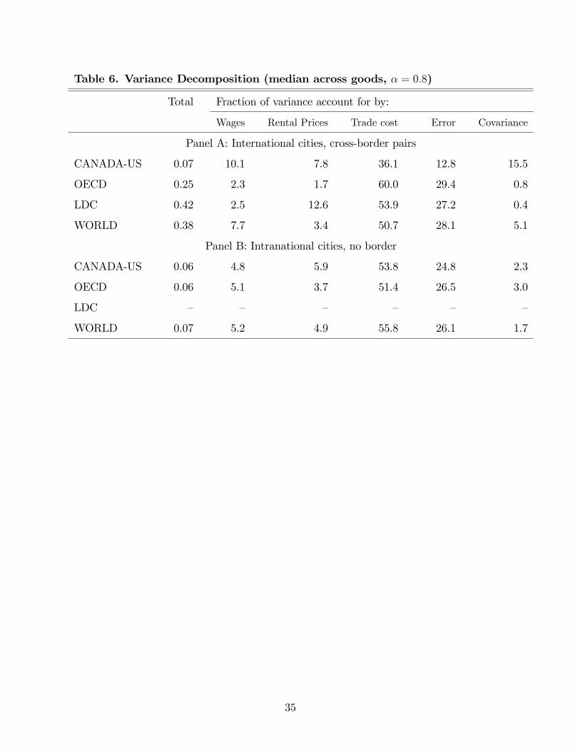
Table 6. Variance Decomposition (median across goods, � = 0:8)

Total Fraction of variance account for by:

Wages Rental Prices Trade cost Error Covariance


CANADA-US 0.07 10.1 7.8 36.1 12.8 15.5

OECD 0.25 2.3 1.7 60.0 29.4 0.8

LDC 0.42 2.5 12.6 53.9 27.2 0.4

WORLD 0.38 7.7 3.4 50.7 28.1 5.1


CANADA-US 0.06 4.8 5.9 53.8 24.8 2.3

OECD 0.06 5.1 3.7 51.4 26.5 3.0

LDC � � � � � �

WORLD 0.07 5.2 4.9 55.8 26.1 1.7

35

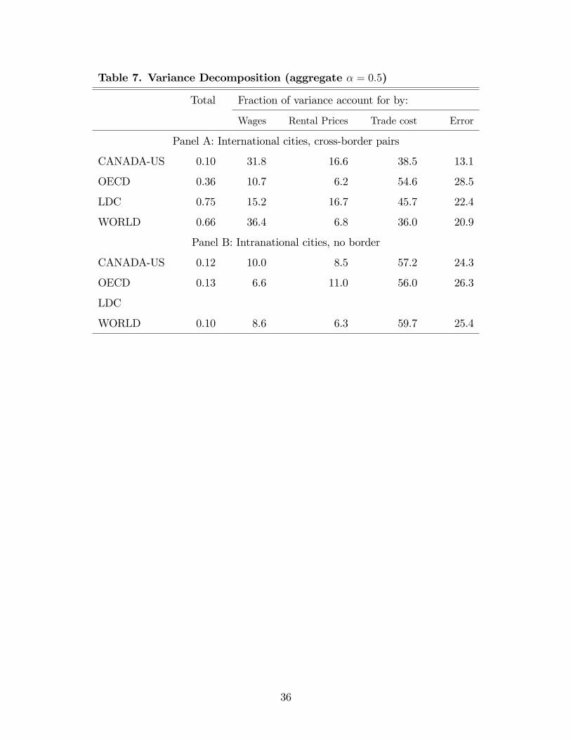
Table 7. Variance Decomposition (aggregate � = 0:5)

Total Fraction of variance account for by:

Wages Rental Prices Trade cost Error


CANADA-US 0.10 31.8 16.6 38.5 13.1

OECD 0.36 10.7 6.2 54.6 28.5

LDC 0.75 15.2 16.7 45.7 22.4

WORLD 0.66 36.4 6.8 36.0 20.9


CANADA-US 0.12 10.0 8.5 57.2 24.3

OECD 0.13 6.6 11.0 56.0 26.3

LDC

WORLD 0.10 8.6 6.3 59.7 25.4

36

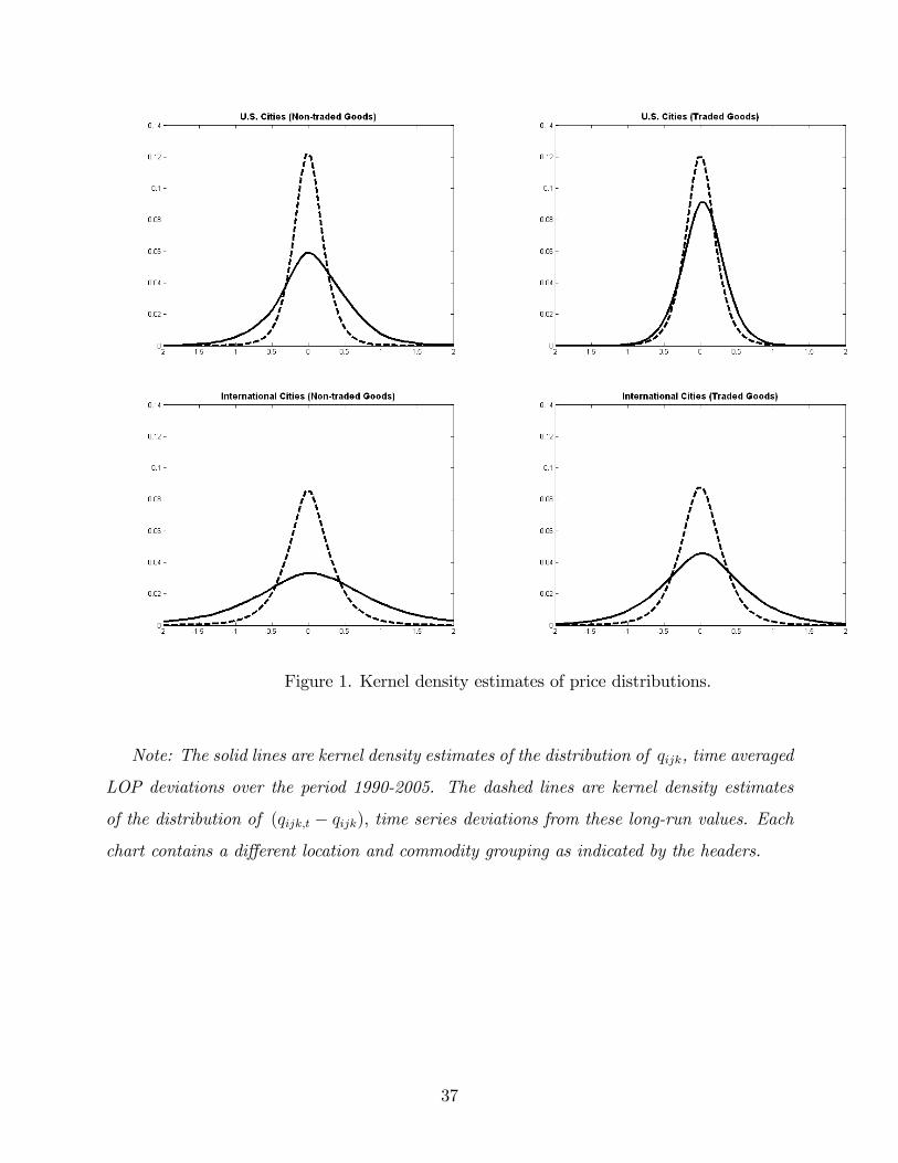
Figure 1. Kernel density estimates of price distributions.

Note: The solid lines are kernel density estimates of the distribution of qijk, time averaged

LOP deviations over the period 1990-2005. The dashed lines are kernel density estimates

of the distribution of (qijk;t � qijk), time series deviations from these long-run values. Each

chart contains a di¤erent location and commodity grouping as indicated by the headers.

37

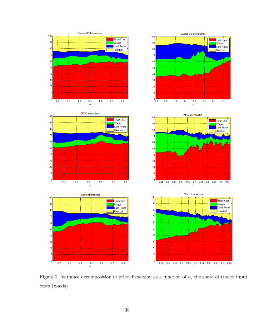
Figure 2. Variance decomposition of price dispersion as a function of �i the share of traded input

costs (x-axis)

38

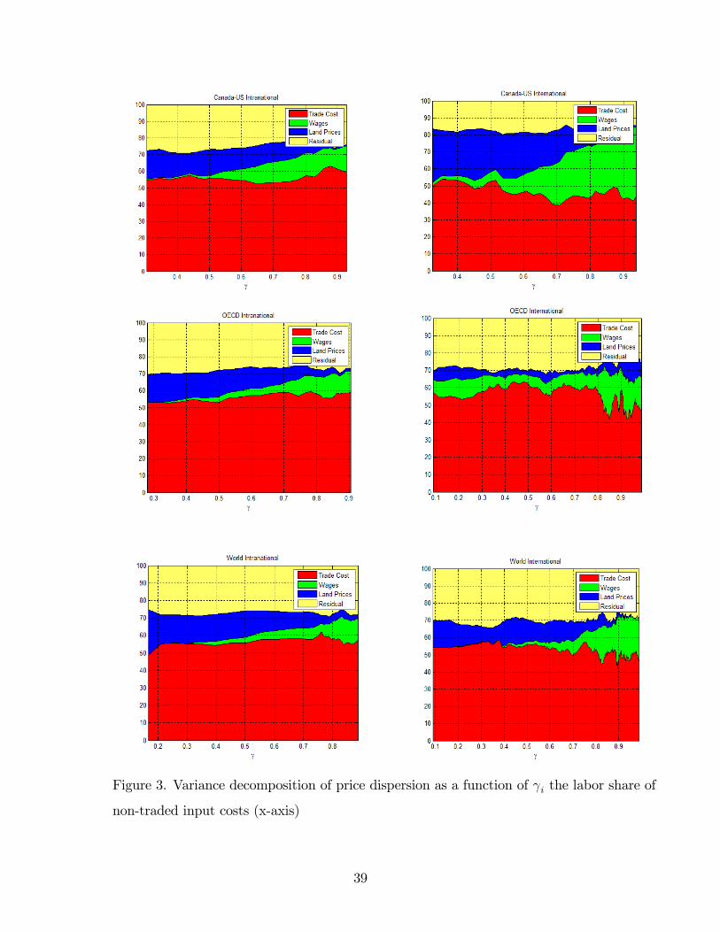
Figure 3. Variance decomposition of price dispersion as a function of i the labor share of

non-traded input costs (x-axis)

39

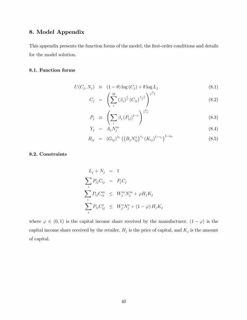
8. Model Appendix

This appendix presents the function forms of the model, the �rst-order conditions and details

for the model solution.

8.1. Function forms

U(Cj; Nj) � (1� �) log (Cj) + � logLj (8.1)

Cj =

MXi

(�i)1" (Cij)

"�1"

! ""�1

(8.2)

Pj � X

i

�i (Pij)1�"

! 11�"

(8.3)

Yj = AjNmj (8.4)

Rij = (Gij)�i��BjN

sij

� i (Kij)1� i

�1��i (8.5)

8.2. Constraints

Lj +Nj = 1Xi

PijCij = PjCjXi

PijCmij � Wm

j Nmj + 'HjKjX

i

PijCsij � W s

jNsj + (1� ')HjKj

where ' 2 (0; 1) is the capital income share received by the manufacturer, (1� ') is the

capital income share received by the retailer, Hj is the price of capital, and Kj is the amount

of capital.

40

8.3. Consumer and producer problems

maxCjf(1� �) log (Cj) + � logLj + �j[Wm

j (1� Lj) + 'HjKj � PjCj]g (8.6)

maxCjf(1� �) log (Cj) + � logLj + �j[W s

j (1� Lj) + (1� ')HjKj � PjCj]g (8.7)

maxNmj

fQjjAjNmj �Wm

j Nmj g (8.8)

maxGi;Ns

j

fPij (Gij)�i��BjN

sij

� i (Kij)1� i

�1��i �QijGij �W sjN

sij �HjKijg (8.9)

8.4. E¢ ciency conditions

CAij = �i

�PijPj

��"CAj (8.10)

CAj =WAj

Pj

(1� �)�

�1�NA

j

�(8.11)

Nmj = 1� � � '�HjKj

Wmj

(8.12)

N sj = 1� � � (1� ') �HjKj

W sj

(8.13)

Lmj = � +'�HjKj

Wmj

(8.14)

Lsj = � +(1� ') �HjKj

W sj

(8.15)

(8.16)

N sij =

(1� �i) i�i

QijW sj

Rij

�BjQijW sj

(1� �i) i�i

�(�i�1) i �QijHj

(1� �i) (1� i)�i

�(�i�1)(1� i)(8.17)

Gij = Rij

�BjQijW sj

(1� �i) i�i


(1� �i) (1� i)�i

�(�i�1)(1� i)(8.18)

Kij =(1� �i) (1� i)

�i

QijHjRij

�BjQijW sj

(1� �i) i�i


(1� �i) (1� i)�i

�(�i�1)(1� i)(8.19)

Qjj = MCj =Wmj

Aj(8.20)

Pij = MCsij =(Qij)

�i��

W sj

Bj

� i(Hj)

(1� i)�(1��i)

��ii

�(1� �i) ( i)

i (1� i)(1� i)

�(1��i) (8.21)

8.5. Price relationships

Qji = (1 + � ji)Qjj (8.22)

41

8.6. The retail �rm

N sj = 1� � �

(1� ') �HjKj

W sj

=Xi

N sij =

Xi

8><>:(1��i) i

�i

QijW sjRij

�BjQijW sj

(1��i) i�i

�(�i�1) ��QijHj

(1��i)(1� i)�i

�(�i�1)(1� i)9>=>;

Gij = Rij

�BjQijW sj

(1� �i) i�i


(1� �i) (1� i)�i

�(�i�1)(1� i)8.7. General equilibrium

8.7.1. Manufacturing Labor Market

The labor supply of the manufacturer is used in the manufacturing process, which implies:

YjAj= 1� � � '�HjKj

Wmj

(8.23)

8.7.2. Goods Market

In the global general equilibrium all the conditions of partial equilibrium must hold. However

we also require that the supply of each good equals the demand for each good. This is where

the treatment of trade costs becomes crucial. We will assume that trade costs are of the

iceberg variety, so the physical resource constraint for good j must satisfy:

Yj =Xi

Gji (1 + � ij) (8.24)

In words: the units produced equal the demand of traded inputs of retailers at the desti-

nations plus a fraction lost to iceberg costs. The aggregate fraction lost will depend on the

equilibrium allocations since the loss along any bilateral trade route is proportional to the

volume of trade along that branch:

TjYj=

PiGji� ijP

iGji (1 + � ij)(8.25)

Returning to our global equilibrium, we substitute the optimal traded input choices of the

retailers into the resource constraint to arrive at:

Yj =Xi

Rji

�BiQjiW si

(1� �j) j�j

�(�j�1) j QjiHi

(1� �j)�1� j

��j

!(�j�1)(1� j)(1 + � ji)

42

Recall 8.23:YjAj= 1� � � '�HjKj

Wmj

Combining these last two we get:

Xi

Rji

�BiQjiW si

(1� �j) j�j


(1� �j)�1� j

��j

!(�j�1)(1� j)(1 + � ji)(8.26)

= Aj

�1� � � '�HjKj

Wmj

�(8.27)

The equilibrium of the retailer implies:

Rij = Cmij + C

sij = �i

�PijPj

��" �Cmj + C

sj

�Assuming that " = 1 (for the rest of the text), we have:

Rij = Cmij + C

sij =

�iPij

�PjC

mj + PjC

sj

�=�iPij

�Nmj W

mj +N

sjW

sj +HjKj

�Rji =

�jPji

(Nmi W

mi +N

siW

si +HiKi)

which says that the total income (sales) of the retailer from good i is equal to the share of

that good in the budget of the region. Thus, we have

Xi

Rji

�BiQjiW si

(1� �j) j�j


(1� �j)�1� j

��j

!(�j�1)(1� j)(1 + � ji)

= Aj

�1� � � '�HjKj

Wmj

�

Xi

8>><>>:�jPji(Nm

i Wmi +N

siW

si +HiKi)

�BiQjiW si

(1��j) j�j

�(�j�1) j��QjiHi

(1��j)(1� j)�j

�(�j�1)(1� j)(1 + � ji)

9>>=>>; = Aj

�1� � � '�HjKj

Wmj

�

Recall the price set by the retailer:

Pij =(Qij)

�i��

W sj

Bj

� i(Hj)

(1� i)�(1��i)

��ii

�(1� �i) ( i)

i (1� i)(1� i)

�(1��i)which is to say:

Pji =(Qji)

�j�W si

Bi

�(1��j) j(Hi)

(1��j)(1� j)

��jj

�(1� �j) j

�(1��j) j �(1� �j) �1� j��(1��j)(1� j)43

Thus,

Xi

8>>>>>><>>>>>>:

�j

(Qji)�j Wsi

Bi

!(1��j) j(Hi)(1��j)(1� j)

��jj ((1��j) j)

(1��j) j((1��j)(1� j))(1��j)(1� j)

(Nmi W

mi +N

siW

si +HiKi)

��BiQjiW si

(1��j) j�j

�(�j�1) j �QjiHi

(1��j)(1� j)�j

�(�j�1)(1� j)(1 + � ji)

9>>>>>>=>>>>>>;= Aj

�1� � � '�HjKj

Wmj

�Xi

�jQji

(Nmi W

mi +N

siW

si +HiKi)�j (1 + � ji) = Aj

�1� � � '�HjKj

Wmj

�By using Qjj =

Wmj

Ajand Qji = (1 + � ji)Qjj, we can write

Xi

�j(1 + � ji)Wm

j

(Nmi W

mi +N

siW

si +HiKi)�j (1 + � ji) =

�1� � � '�HjKj

Wmj

�

�j�jXi

(Nmi W

mi +N

siW

si +HiKi) =W

mj

�1� � � '�HjKj

Wmj

��j�j

Xi

(Nmi W

mi +N

siW

si +HiKi) =W

mj N

mj (8.28)

This is the �rst equation for the relation between NmWm, N sW s, and HK.

8.7.3. Retailing Labor Market

We have the following condition for the retailing labor market equilibrium:

N sj =

Xi

N sij =

Xi

8><>:(1��i) i

�i

QijW sjRij

�BjQijW sj

(1��i) i�i


(1��i)(1� i)�i

�(�i�1)(1� i)9>=>;

N sj =

Xi

8>>>><>>>>:(1��i) i

�i

QijW sj

�i(Nmj W

mj +N

sjW

sj +HjKj)

(Qij)�i Wsj

Bj

!(1��i) i(Hj)

(1��i)(1� i)

��ii ((1��i) i)

(1��i) i ((1��i)(1� i))(1��i)(1� i)

��BjQijW sj

(1��i) i�i


(1��i)(1� i)�i

�(�i�1)(1� i)9>>>>=>>>>;

N sjW

sj =

�Nmj W

mj +N

sjW

sj +HjKj

�Xi

(1� �i) i�i (8.29)

This is the second equation for the relation between NmWm, N sW s, and HK.

44

8.7.4. Capital Market

We have the following condition for the capital market equilibrium:

Kj =Xi

Kij =Xi

8><>:(1��i)(1� i)

�i

QijHjRij

�BjQijW sj

(1��i) i�i


(1��i)(1� i)�i

�(�i�1)(1� i)9>=>;

HjKj =�Nmj W

mj +N

sjW

sj +HjKj

�Xi

(1� �i) (1� i) �i (8.30)

This is the third equation for the relation between NmWm, N sW s, and HK.

8.7.5. Implications for Wages, Rents, Wage Income, and Capital Income

Recall 8.28, 8.29, 8.30, which are:

Nmj W

mj = �j�j

Xi

(Nmi W

mi +N

siW

si +HiKi)

N sjW

sj =

�Nmj W

mj +N

sjW

sj +HjKj

�Xi

(1� �i) i�i

HjKj =�Nmj W

mj +N

sjW

sj +HjKj

�Xi

(1� �i) (1� i) �i

Combine 8.29 and 8.30 to get:

HjKj

N sjW

sj

=

Pi (1� �i) (1� i) �iP

i (1� �i) i�i(8.31)

and �HjKj +N

sjW

sj

�= Nm

j Wmj

Pi (1� �i) �i

(1�P

i (1� �i) �i)(8.32)

and thusN sjW

sj

Nmj W

mj

=

Pi (1� �i) i�i

(1�P

i (1� �i) �i)(8.33)

which show that the sectoral wage incomes and capital incomes are all proportional to each

other within each city.

Recall the individual optimality condition for the retailer:

N sj = 1� � �

(1� ') �HjKj

W sj

N sjW

sj = W

sj (1� �)� (1� ') �HjKj

45

Combine this with 8.31 to get:

HjKj =

�N sjW

sj

�Pi (1� �i) (1� i) �iP

i (1� �i) i�i

N sjW

sj

�1 +

(1� ') �P

i (1� �i) (1� i) �iPi (1� �i) i�i

�= W s

j (1� �)

N sj =

(1� �)P

i (1� �i) i�i(P

i (1� �i) i�i) + (1� ') � (P

i (1� �i) (1� i) �i)(8.34)

which shows that N sj is constant across regions. In a special case in which the share of

capital is equal to zero in the retail production function (i.e., i = 0), or in which the share

of capital income received by the retailer is equal to zero (i.e., ' = 1), we have N sj = (1� �).

Combine 8.33 with 8.28 to get:

NsjW

sj (1�

Pi(1��i)�i)P

i(1��i) i�iNskW

sk(1�

Pi(1��i)�i)P

i(1��i) i�i

=Nmj W

mj

Nmk W

mk

=�j�j�k�k

=N sjW

sj

N skW

sk

which show that the manufacturing wage income and the retailing wage income are propor-

tional across cities. It is implied that:

W sj

W sk

=�j�j�k�k

(8.35)

since N sj is constant across regions. If we also use 8.31, we obtain:

HjKj

HkKk

=�j�j�k�k

(8.36)

where KA is the capital stock in city A = j; k.

Recall the individual optimality conditions for both the retailer and the manufacturer:

Wmj N

mj = Wm

j (1� �)� '�HjKj

W sjN

sj = W s

j (1� �)� (1� ') �HjKj

These conditions can be combined to obtain:

Wmj

W sj

=' (1� �)� 'N s

j

(1� ') (1� �)� (1� ')Nmj

46

Recall 8.33:Nmj W

mj

N sjW

sj

=(1�

Pi (1� �i) �i)P

i (1� �i) i�iCombine the last two expressions to get:

Nmj W

mj

N sjW

sj

=Nmj

N sj

' (1� �)� 'N sj

(1� ') (1� �)� (1� ')Nmj

=(1�

Pi (1� �i) �i)P

i (1� �i) i�i

Nmj

�' (1� �)N sj

� '�X

i

(1� �i) i�i

= (1� ') (1� �) 1�

Xi

(1� �i) �i

!� (1� ')Nm

j

1�

Xi

(1� �i) �i

!which can be combined with 8.34 (i.e., N s

j ) to obtain:

Nmj = (1� �)� '� (�0 � �1) (1� �)

'� (�0 � �1) + (1� �0)= (1� �) when ' = 0 or i = 1

where �0 �P

i (1� �i) �i, �1 �P

i (1� �i) i�i, �0 � �1 =P

i (1� �i) (1� i) �i.�2 �Pi �i�i = 1��0. This shows that Nm

j is constant and equal across cities. The level of e¤ort

is equal to the leisure share of expenditure, (1� �) when either rental income is zero for the

manufacturer (' = 0) or when retail production is labor-only i = 1. E¤ort is declining in

asset income.

Nmj

(1� �) = 1� '� (�0 � �1)'� (�0 � �1) + (1� �0)

@Nmj

(1��)

@'= �� (�0 � �1) d�1 + '� (�0 � �1) d�2

= � (�0 � �1) d�1[�1 + 'd�1]

sign@Nmj

(1��)

@'= sign [�1 + 'd�1] since � (�0 � �1) d�1 > 0

' < d

Nmj =

(1� �0) (1� �)(1� �0) + '� (�0 � �1)

N sj =

�1 (1� �)�1 + (1� ') � (�0 � �1)

47

Wmj

W sj

=(1� �0) + '� (�0 � �1)

(1� ') (1� �) (1� �0) + '� (�0 � �1)� (1� ')(1� ') � (�0 � �1)

�1 + (1� ') � (�0 � �1)

8.8. Implications for Price Ratios across Cities

Recall the retail price of good i in city j and city k:

Pij =(Qij)

�i�W sj

Bj

�(1��i) i(Hj)

(1��i)(1� i)

��ii ((1� �i) i)(1��i) i ((1� �i) (1� i))

(1��i)(1� i)

Pik =(Qik)

�i�W sk

Bk

�(1��i) i(Hk)

(1��i)(1� i)

��ii ((1� �i) i)(1��i) i ((1� �i) (1� i))

(1��i)(1� i)

Take their ratio to get:

PijPik

=(Qij)

�i�W sj

Bj

�(1��i) i(Hj)

(1��i)(1� i)

(Qik)�i�W sk

Bk

�(1��i) i(Hk)

(1��i)(1� i)

By using Qij = (1 + � ij)Qii, we can write the ratio of the price of good i across regions j

and k as follows:

PijPik

=((1 + � ij))

�i

((1 + � ik))�i

�W sj

Bj

�(1��i) i(Hj)

(1��i)(1� i)�W sk

Bk

�(1��i) i(Hk)

(1��i)(1� i)

By using 8.35 and 8.36, the analytical solution for the price ratios can be written as:

PijPik

=

��BkBj

� i �j�j�k�k

�(1��i)�1 + � ij1 + � ik

��i �Kk

Kj

�(1��i)(1� i)where Kj is the total amount of capital in city j.

9. Estimation Appendix

The derivation of the variance decomposition of equation 5.6 can be written as follows:

varjk [Et (qijk;t)] = varjk [(1� b�i) b iEt (!jk;t)] + varjk [(1� b�i) (1� b i)Et (hjk;t)]+varjk

hb�iEt �bIijk;tb�idjk�i+ varjk [Et (b"ijk;t)]+2cov ((1� b�i) b iEt (!jk;t) ; (1� b�i) (1� b i)Et (hjk;t))+2cov

�(1� b�i) b iEt (!jk;t) ; b�iEt �bIijk;tb�idjk��

+2cov�(1� b�i) (1� b i)Et (hjk;t) ; b�iEt �bIijk;tb�idjk��

48

where b�i�s, b i�s, bIijk�s, b�i�s and b"ijk�s are all estimated values for the relevant variables. Notethat the covariance terms including Et (b"ijk;t) are equal to zero by OLS regression.

49

Documents

NATIONAL BUREAU OF ECONOMIC RESEARCH IMPLICATIONS …