N87 -10365CALIBRATION AND ANALYSIS FOR A 0.53 pm INCOHERENT DOPPLER LIDAR

J. Sroga and A. Rosenberg

RCA Astro-E1ectronics

P. O. Box 800

Princeton, gJ 08540

I. Introduction

Asround based, prototype Doppler lidar is being developed to demonstrate

the feasibility of an incoherent detection technique to remotely measurewinds in the atmosphere. This prototype system consists of a narrow-

band, single-frequency laser transmitter, a high-resolution, Fabry-Perot

Interferometer (FPI) utilizing a multichannel Image Plane Detector (IPD)

and a data acquisition system. A description of the prototype Doppler

lidar hardware is given in Rosenberg and Sroga, 1985. This paper will

describe the calibration and analysis procedures for this system.

Preliminary results from data obtained with the system pointed verticallywill be presented.

II. Instrument Calibration

The signal intensity measured in each channel of the FPI-IPD Dopplerlidar is the convolution of the spectral distribution of the source (e.g.

laser or atmospheric backscatter) with the instrument transmission

function for that particular channel. The instrument functions, which

contain information of the spectral broadening effects and the relative

IPD channel sensitivities, are obtained by a wavelength scan of the

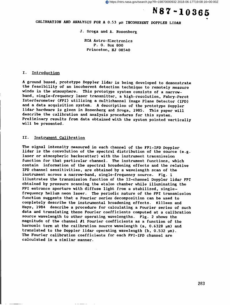
instrument across a narrow-band, single-frequency source. Fig. 1

illustrates the transmission function of the 12-channel Doppler lidar FPI

obtained by pressure scanning the etalon chamber while illuminating the

FPI entrance aperture with diffuse light from a stabilized, single-

frequency helium neon laser. The periodic nature of the FPI transmission

function suggests that a Fourier series decomposition can be used to

completely describe the instrumental broadening effects. Killeen and

Hays, 1984 describe a procedure for calculating a Fourier series of such

data and translating these Fourier coefficients computed at a calibration

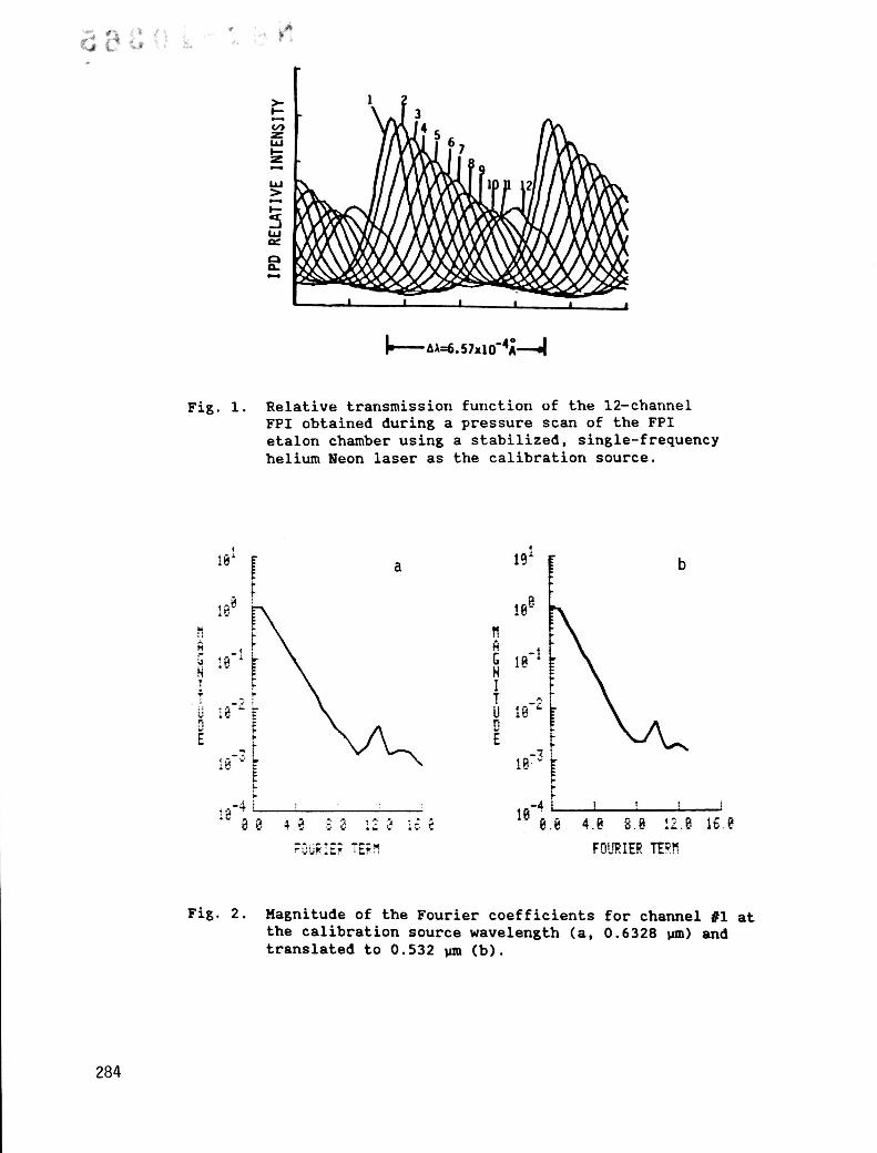
source wavelength to other operating wavelengths. Fig. 2 shows the

magnitude of the channel #I Fourier coefficients as a function of the

harmonic term at the calibration source wavelength (a, 0.6328 _m) and

translated to the Doppler lidar operating wavelength (b, 0.532 _m).

The Fourier calibration coefficients for each FPI-IPD channel are

calculated in a similar manner.

283

https://ntrs.nasa.gov/search.jsp?R=19870000932 2018-06-17T19:08:16+00:00Z

I I I 1 1

Fig. 1. Relative transmission function of the 12-channel FPI obtained during a pressure scan of the FPI etalon chamber using a stabilized, single-frequency helium Neon laser as the calibration source.

a

t *

lql f b

Fig. 2. Magnitude of the Fourier coefficients for channel #l at the calibration source wavelength (a, 0.6328 run) and translated to 0.532 pm (b).

284

III. Data Analysis

The Fourier calibration coefficients calculated from the above procedureare combined with an analytical description of the FPI and the

atmospheric backscatter spectra to form a model of the Doppler lidarbackscattered signals. This instrument model is a nonlinear function of

the system design parameters and the Fourier calibration coefficients,

which are the system constants, and variable parameters as the total

aerosol and molecular backscatter intensities and the mean atmospheric

Doppler shift velocity. A nonlinear regression technique (Draper and

Smith, 1981), which is similar to the matrix technique of Killeen and

Hays, 1984, is used to adjust these variable model parameters to yield a

"best fit" of the model to the measured FPI-IPD intensities, andtherefore optimum values for these parameters.

Preliminary atmospheric testing with the 0.53 pm Doppler lidar has

been conducted to demonstrate the system capabilities. The calibration

and analysis procedures have been applied to this data to derive the mean

Doppler shift and separate the total aerosol and molecular backscatter

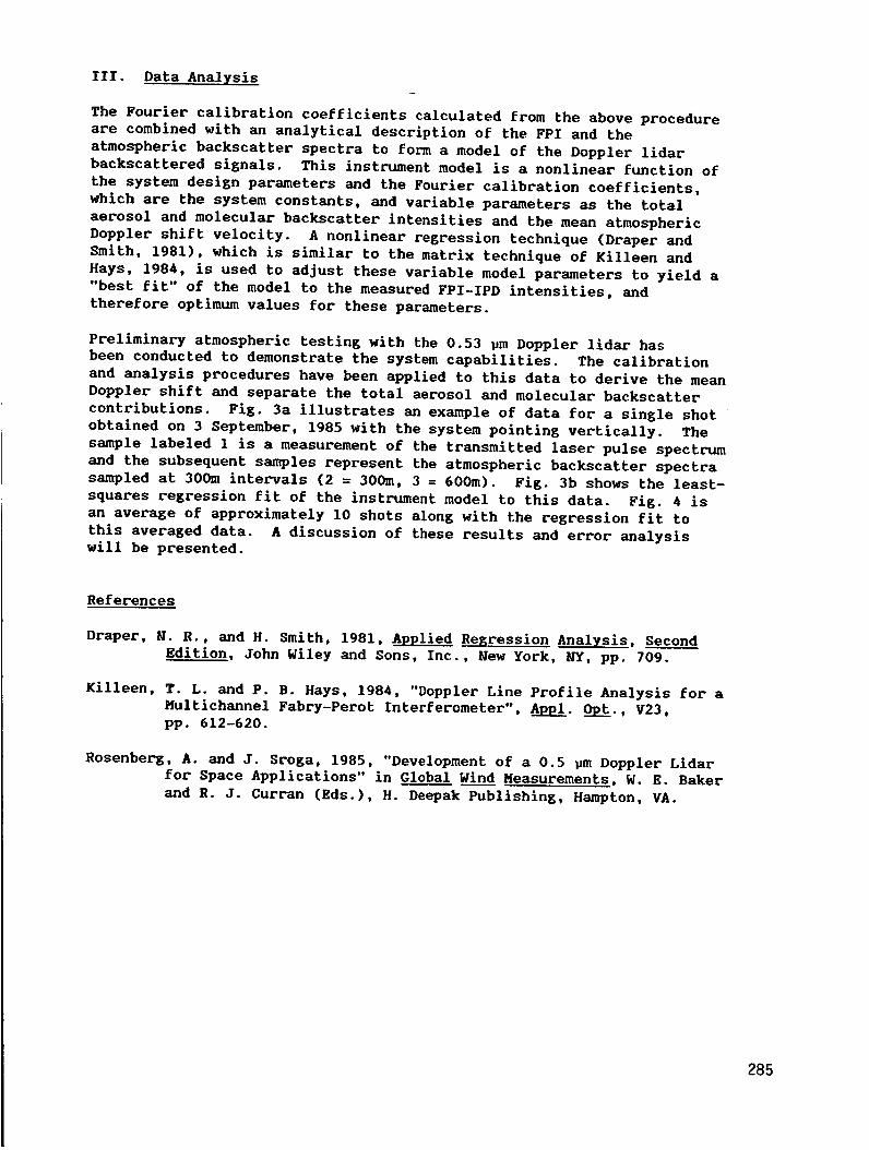
contributions. Fig. 3a illustrates an example of data for a single shot

obtained on 3 September, 1985 with the system pointing vertically. The

sample labeled 1 is a measurement of the transmitted laser pulse spectrum

and the subsequent samples represent the atmospheric backscatter spectra

sampled at 300m intervals (2 = 300m, 3 = 600m). Fig. 3b shows the least-

squares regression fit of the instrument model to this data. Fig. 4 is

an average of approximately 10 shots along with the regression fit to

this averaged data. A discussion of these results and error analysis

will be presented.

References

Draper, N. R., and H. Smith, 1981, Applied Regression Analysis, Second

Edition, John Wiley and Sons, Inc., New York, MY, pp. 709.

KiUeen, T. L. and P. B. Hays, 1984, "Doppler Line Profile Analysis for a

Multichannel Fabry-Perot Interferometer", Appl. Opt., V23,

pp. 612-620.

Rosenberg, A. and J. Sroga, 1985, "Development of a 0.5 pm Doppler Lidar

for Space Applications" in Global Wind Measurements, W. E. Baker

and R. J. Curran (Eds.), H. Deepak Publishing, Hampton, VA.

285

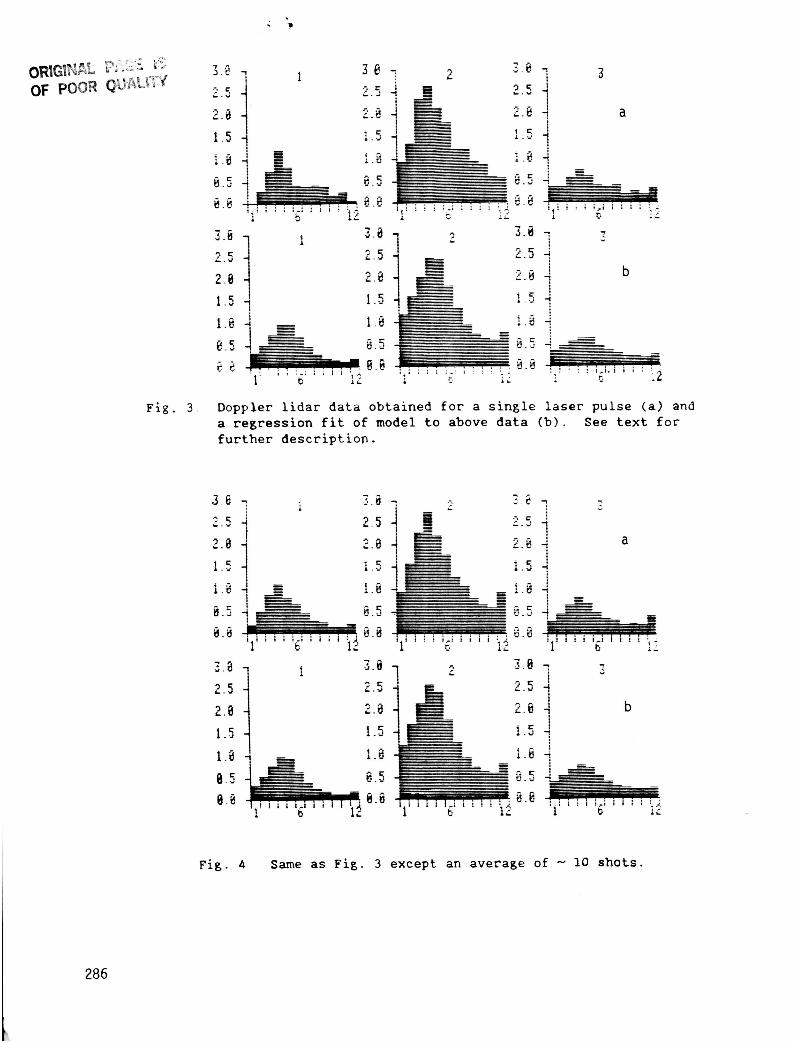
Fig . 3 . Doppler l i d a r data obtained for a s i n g l e laser pulse (a) and a regress ion f i t of model to above data ( b ) . See t e x t f o r further descr ipt ion.

F i g . 4 Same a s F i g . 3 except an average of - 10 shot s .