Embed Size (px)
Citation preview

Musical L-Systems
Stelios ManousakisJune 2006Master’s Thesis - SonologyThe Royal Conservatory, The Hague
1

Abstract
This dissertation presents an extensive framework for designing Lindenmayer systems that generate musical structures. The algorithm is a recursive, biologically inspired string rewriting system in the form of a formal grammar, which can be used in a variety of different fields. The various sub-categories of L-systems are presented, following a review of the musical applications by other reaserchers. A new model for musical L-systems is shown, based on the author’ s implementation in Max/MSP/Jitter. The focus is on the musical interpretation and mapping of the generated data for electronic music, as well as in expanding the basic model to include various types of control schemata. Some compositional strategies are suggested for generating musical structures from the macro- level to the sample level, supported by a number of audio examples.
3

Aknowledgements
I would like to thank :
My mentor Joel Ryan for his inspiring lectures, advice and support throughout my studies at the Institute of Sonology, as well as for his comments on this dissertation.
Paul Berg, for his valuable help as a reader of this dissertation.
All my teachers and fellow students at the Institute of Sonology for creating such an inspiring environment.
Stephanie, for her love and support, her linguistic and semantic help in this paper, as well as for her irreplacable contribution to my musical work as a singer.
My family for their continuous and never ending support.
4
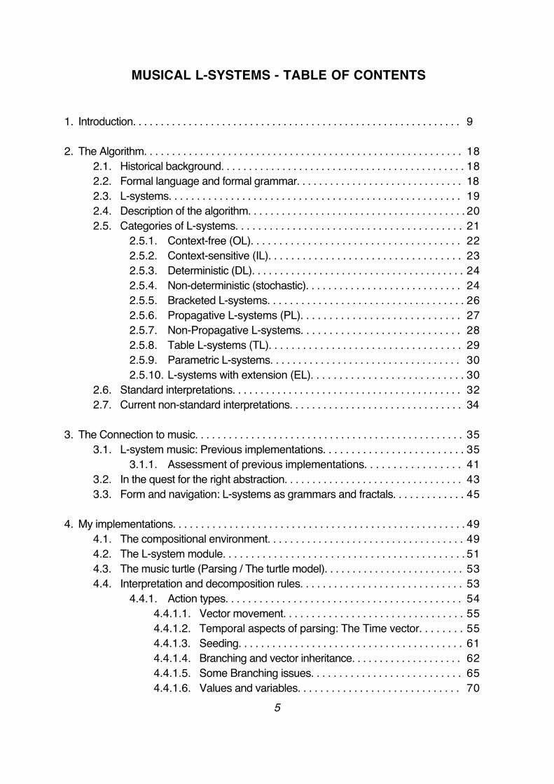
MUSICAL L-SYSTEMS - TABLE OF CONTENTS
1. Introduction. . . . . . . . . . . . . . . . . . . . . . . . . . . . . . . . . . . . . . . . . . . . . . . . . . . . . . . . . . . 9
2. The Algorithm. . . . . . . . . . . . . . . . . . . . . . . . . . . . . . . . . . . . . . . . . . . . . . . . . . . . . . . . . 182.1. Historical background. . . . . . . . . . . . . . . . . . . . . . . . . . . . . . . . . . . . . . . . . . . . 182.2. Formal language and formal grammar. . . . . . . . . . . . . . . . . . . . . . . . . . . . . . 18 2.3. L-systems. . . . . . . . . . . . . . . . . . . . . . . . . . . . . . . . . . . . . . . . . . . . . . . . . . . . 192.4. Description of the algorithm. . . . . . . . . . . . . . . . . . . . . . . . . . . . . . . . . . . . . . . 202.5. Categories of L-systems. . . . . . . . . . . . . . . . . . . . . . . . . . . . . . . . . . . . . . . . 21
2.5.1. Context-free (OL). . . . . . . . . . . . . . . . . . . . . . . . . . . . . . . . . . . . . 222.5.2. Context-sensitive (IL). . . . . . . . . . . . . . . . . . . . . . . . . . . . . . . . . . 232.5.3. Deterministic (DL). . . . . . . . . . . . . . . . . . . . . . . . . . . . . . . . . . . . . . 242.5.4. Non-deterministic (stochastic). . . . . . . . . . . . . . . . . . . . . . . . . . . . 242.5.5. Bracketed L-systems. . . . . . . . . . . . . . . . . . . . . . . . . . . . . . . . . . . 262.5.6. Propagative L-systems (PL). . . . . . . . . . . . . . . . . . . . . . . . . . . . 272.5.7. Non-Propagative L-systems. . . . . . . . . . . . . . . . . . . . . . . . . . . . 282.5.8. Table L-systems (TL). . . . . . . . . . . . . . . . . . . . . . . . . . . . . . . . . . 292.5.9. Parametric L-systems. . . . . . . . . . . . . . . . . . . . . . . . . . . . . . . . . . 302.5.10. L-systems with extension (EL). . . . . . . . . . . . . . . . . . . . . . . . . . . 30
2.6. Standard interpretations. . . . . . . . . . . . . . . . . . . . . . . . . . . . . . . . . . . . . . . . . 322.7. Current non-standard interpretations. . . . . . . . . . . . . . . . . . . . . . . . . . . . . . . 34
3. The Connection to music. . . . . . . . . . . . . . . . . . . . . . . . . . . . . . . . . . . . . . . . . . . . . . . . 353.1. L-system music: Previous implementations. . . . . . . . . . . . . . . . . . . . . . . . . 35
3.1.1. Assessment of previous implementations. . . . . . . . . . . . . . . . . 413.2. In the quest for the right abstraction. . . . . . . . . . . . . . . . . . . . . . . . . . . . . . . . 433.3. Form and navigation: L-systems as grammars and fractals. . . . . . . . . . . . . 45
4. My implementations. . . . . . . . . . . . . . . . . . . . . . . . . . . . . . . . . . . . . . . . . . . . . . . . . . . . 494.1. The compositional environment. . . . . . . . . . . . . . . . . . . . . . . . . . . . . . . . . . . 494.2. The L-system module. . . . . . . . . . . . . . . . . . . . . . . . . . . . . . . . . . . . . . . . . . . 514.3. The music turtle (Parsing / The turtle model). . . . . . . . . . . . . . . . . . . . . . . . . 534.4. Interpretation and decomposition rules. . . . . . . . . . . . . . . . . . . . . . . . . . . . . 53
4.4.1. Action types. . . . . . . . . . . . . . . . . . . . . . . . . . . . . . . . . . . . . . . . . . 544.4.1.1. Vector movement. . . . . . . . . . . . . . . . . . . . . . . . . . . . . . . . 554.4.1.2. Temporal aspects of parsing: The Time vector. . . . . . . . 554.4.1.3. Seeding. . . . . . . . . . . . . . . . . . . . . . . . . . . . . . . . . . . . . . . . 614.4.1.4. Branching and vector inheritance. . . . . . . . . . . . . . . . . . . . 624.4.1.5. Some Branching issues. . . . . . . . . . . . . . . . . . . . . . . . . . . 654.4.1.6. Values and variables. . . . . . . . . . . . . . . . . . . . . . . . . . . . . 70
5
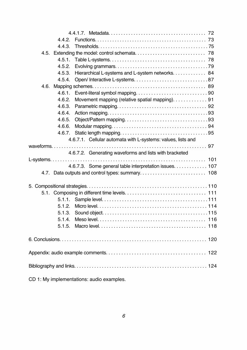
4.4.1.7. Metadata. . . . . . . . . . . . . . . . . . . . . . . . . . . . . . . . . . . . . . . 724.4.2. Functions. . . . . . . . . . . . . . . . . . . . . . . . . . . . . . . . . . . . . . . . . . . . . 734.4.3. Thresholds. . . . . . . . . . . . . . . . . . . . . . . . . . . . . . . . . . . . . . . . . . . . 75
4.5. Extending the model: control schemata. . . . . . . . . . . . . . . . . . . . . . . . . . . . 784.5.1. Table L-systems. . . . . . . . . . . . . . . . . . . . . . . . . . . . . . . . . . . . . . 784.5.2. Evolving grammars. . . . . . . . . . . . . . . . . . . . . . . . . . . . . . . . . . . . . 794.5.3. Hierarchical L-systems and L-system networks. . . . . . . . . . . . . 844.5.4. Open/ Interactive L-systems. . . . . . . . . . . . . . . . . . . . . . . . . . . . . 87
4.6. Mapping schemes. . . . . . . . . . . . . . . . . . . . . . . . . . . . . . . . . . . . . . . . . . . . . 894.6.1. Event-literal symbol mapping. . . . . . . . . . . . . . . . . . . . . . . . . . . . 904.6.2. Movement mapping (relative spatial mapping). . . . . . . . . . . . . 914.6.3. Parametric mapping. . . . . . . . . . . . . . . . . . . . . . . . . . . . . . . . . . . . 924.6.4. Action mapping. . . . . . . . . . . . . . . . . . . . . . . . . . . . . . . . . . . . . . . . 934.6.5. Object/Pattern mapping. . . . . . . . . . . . . . . . . . . . . . . . . . . . . . . . . 934.6.6. Modular mapping. . . . . . . . . . . . . . . . . . . . . . . . . . . . . . . . . . . . . . 944.6.7. Static length mapping. . . . . . . . . . . . . . . . . . . . . . . . . . . . . . . . . . . 95
4.6.7.1. Cellular automata with L-systems: values, lists and waveforms. . . . . . . . . . . . . . . . . . . . . . . . . . . . . . . . . . . . . . . . . . . . . . . . . . . . . . . . . . . . . . 97
4.6.7.2. Generating waveforms and lists with bracketed L-systems. . . . . . . . . . . . . . . . . . . . . . . . . . . . . . . . . . . . . . . . . . . . . . . . . . . . . . . . . . . . . . 101
4.6.7.3. Some general table interpretation issues. . . . . . . . . . . . . 1074.7. Data outputs and control types: summary. . . . . . . . . . . . . . . . . . . . . . . . . . 108
5. Compositional strategies. . . . . . . . . . . . . . . . . . . . . . . . . . . . . . . . . . . . . . . . . . . . . . . . 1105.1. Composing in different time levels. . . . . . . . . . . . . . . . . . . . . . . . . . . . . . . . 111
5.1.1. Sample level. . . . . . . . . . . . . . . . . . . . . . . . . . . . . . . . . . . . . . . . . . 1115.1.2. Micro level. . . . . . . . . . . . . . . . . . . . . . . . . . . . . . . . . . . . . . . . . . . . 1145.1.3. Sound object. . . . . . . . . . . . . . . . . . . . . . . . . . . . . . . . . . . . . . . . . . 1155.1.4. Meso level. . . . . . . . . . . . . . . . . . . . . . . . . . . . . . . . . . . . . . . . . . . 1165.1.5. Macro level. . . . . . . . . . . . . . . . . . . . . . . . . . . . . . . . . . . . . . . . . . . 118
6. Conclusions. . . . . . . . . . . . . . . . . . . . . . . . . . . . . . . . . . . . . . . . . . . . . . . . . . . . . . . . . . . 120
Appendix: audio example comments. . . . . . . . . . . . . . . . . . . . . . . . . . . . . . . . . . . . . . . 122
Bibliography and links. . . . . . . . . . . . . . . . . . . . . . . . . . . . . . . . . . . . . . . . . . . . . . . . . . . . . 124
CD 1: My implementations: audio examples.
6
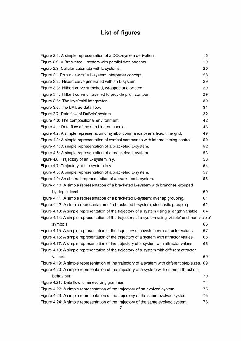
List of figures
Figure 2.1: A simple representation of a DOL-system derivation. 15Figure 2.2: A Bracketed L-system with parallel data streams. 19Figure 2.3. Cellular automata with L-systems. 20Figure 3.1 Prusinkiewicz’ s L-system interpreter concept. 28Figure 3.2: Hilbert curve generated with an L-system. 29Figure 3.3: Hilbert curve stretched, wrapped and twisted. 29Figure 3.4: Hilbert curve unravelled to provide pitch contour. 29Figure 3.5: The lsys2midi interpreter. 30Figure 3.6: The LMUSe data flow. 31Figure 3.7: Data flow of DuBois’ system. 32Figure 4.0: The compositional environment. 42Figure 4.1: Data flow of the stm.Linden module. 43Figure 4.2: A simple representation of symbol commands over a fixed time grid. 49Figure 4.3: A simple representation of symbol commands with internal timing control. 50Figure 4.4: A simple representation of a bracketed L-system. 52Figure 4.5: A simple representation of a bracketed L-system. 53Figure 4.6: Trajectory of an L- system in y. 53Figure 4.7: Trajectory of the system in y. 54Figure 4.8: A simple representation of a bracketed L-system. 57Figure 4.9: An abstract representation of a bracketed L-system. 58Figure 4.10: A simple representation of a bracketed L-system with branches grouped
by depth level . 60Figure 4.11: A simple representation of a bracketed L-system; overlap grouping. 61Figure 4.12: A simple representation of a bracketed L-system; stochastic grouping. 62Figure 4.13: A simple representation of the trajectory of a system using a length variable. 64Figure 4.14: A simple representation of the trajectory of a system using ‘visible’ and ‘non-visible’
symbols. 66Figure 4.15: A simple representation of the trajectory of a system with attractor values. 67Figure 4.16: A simple representation of the trajectory of a system with attractor values. 68Figure 4.17: A simple representation of the trajectory of a system with attractor values. 68Figure 4.18: A simple representation of the trajectory of a system with different attractor
values. 69Figure 4.19: A simple representation of the trajectory of a system with different step sizes. 69Figure 4.20: A simple representation of the trajectory of a system with different threshold
behaviour. 70FIgure 4.21: Data flow of an evolving grammar. 74Figure 4.22: A simple representation of the trajectory of an evolved system. 75Figure 4.23: A simple representation of the trajectory of the same evolved system. 75Figure 4.24: A simple representation of the trajectory of the same evolved system. 76
7
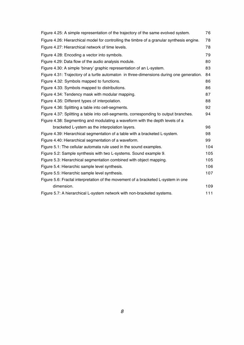
Figure 4.25: A simple representation of the trajectory of the same evolved system. 76Figure 4.26: Hierarchical model for controlling the timbre of a granular synthesis engine. 78Figure 4.27: Hierarchical network of time levels. 78
Figure 4.28: Encoding a vector into symbols. 79Figure 4.29: Data flow of the audio analysis module. 80Figure 4.30: A simple ‘binary’ graphic representation of an L-system. 83Figure 4.31: Trajectory of a turtle automaton in three-dimensions during one generation. 84Figure 4.32: Symbols mapped to functions. 86Figure 4.33: Symbols mapped to distributions. 86Figure 4.34: Tendency mask with modular mapping. 87Figure 4.35: Different types of interpolation. 88Figure 4.36: Splitting a table into cell-segments. 92Figure 4.37: Splitting a table into cell-segments, corresponding to output branches. 94Figure 4.38: Segmenting and modulating a waveform with the depth levels of a
bracketed L-ystem as the interpolation layers. 96Figure 4.39: Hierarchical segmentation of a table with a bracketed L-system. 98Figure 4.40: Hierarchical segmentation of a waveform. 99Figure 5.1: The cellular automata rule used in the sound examples. 104Figure 5.2: Sample synthesis with two L-systems. Sound example 9. 105Figure 5.3: Hierarchical segmentation combined with object mapping. 105Figure 5.4: Hierarchic sample level synthesis. 106Figure 5.5: Hierarchic sample level synthesis. 107Figure 5.6: Fractal interpretation of the movement of a bracketed L-system in one
dimension. 109Figure 5.7: A hierarchical L-system network with non-bracketed systems. 111
8
▼ Chapter 1: Introduction.
Our environment, whether natural or artificial, is filled with sound waves. Due to its propagative nature, sound is a medium that permits information to travel fast and far. Sound is a key for survival. Perceiving and comprehending a sound from the environment gives precious information about it (food, threat, etc.). Producing a sound transmits information to the environment, allowing the individual to interact with it without physical contact.
Organising sound was, possibly, one of the major achievements of the human species, allowing us to communicate by mapping a sound to a sign via a common code. The actual form of a code is dependant on a number of factors, such as: 1) Properties of the medium, or how the message travels. 2) Properties of the users; that is: a) The capacity of the transmitter to form an interpretable message. For this, knowledge of the code is required, as well as the mechanical and cognitive skills to produce a correct message. b)The capacity of the receiver to perceive and understand the code. Knowledge of the code, as well as some perceptual and cognitive skills concerning the medium are necessary. 3) The function of the code. 4) Cultural group history. If any of these factors changes, the code will inevitably change as well.
Established sonic codes can be grouped into two basic categories, both considered to be inherent human capacities with universal distribution in human societies: language and music. The two families share a lot of perceptual and cognitive modules but serve different functions and, as systems, they are essentially different. Shortly, language refers to the world outside it. The fundamental aim of the code is to transmit and communicate the sign. As such, the syntax exists, mainly, to underline and clarify ‘real world’ semantics. Music, on the other hand, is autoreferential with two layers of self-reference: a) the macro- time, refering to the cultural and musical context of the society and of the composer producing a given musical piece; b) the in-music time, refering to the musical context of the piece itself. The core of the meaning of a musical utterance is found on its discourse and interaction with both time levels, which form the musical ‘real world’ of a piece, as expressed by the sequencing of sounds in time. In addition, the mechanical limitations of sound production that apply to language do not apply to music, since objects can be used to produce musical sounds besides the human voice. Different sound generators require different strategies for making ‘meaningful’ sounds according to their mechanics. New sound generators will cause new strategies to be invented. However, these strategies have to be incorporated in the already existing musical model
9
to make sense. The descriptive weight of the code has to shift towards an abstraction that allows incorporating a variety of different sound producing mechanisms (instruments) without having to redefine the framework (the musical idiom). That is, the focus of a code is on the perceived outcome and not on the required mechanical process.
The semantic field of music can be conceived as the multidimensional parameter space of sound perception. In order to interpolate from this multidimensionality to an encodable set of organising principals an abstract code has to evolve, consisting of an alphabet and a set of (preference) rules or accepted strategies for using the alphabet. The alphabet is the set of perceived semantic elements in the code, with words representing semantic states. In a musical idiom, semantic states are sonic states, which the code can explicitly describe and reproduce. A sonic state can be described with a number of perceptual parameters whose existence the conceptual model of the code recognises as lying in its semantic field.
The musical field can, thus, be described as a parameter space - with duration, loudness, pitch and timbre being its vectors. Categorisation is a key for human perception and cognition. A space has to be divided into a functional and economic (meaning easy to perceive and remember) set of meaningful states. As such, in every traditional musical idiom, a grid or reference frame is used to define the boundaries between different states in a perceptual vector. This grid is either absolute, defining specific areas in the vector - like in the case of the different tuning systems for the pitch- or relative -e.g. using powers of two to define the relative duration of notes according to the current tempo.
In order to navigate in any kind of space a strategy is needed. Because of the social character of musical behaviour, this strategy is greatly dependant on history, culture, science and technology. In a given society, certain places in the musical space and certain trajectories have acquired a meaning of their own, relatively common to all the members of the society. A navigation in the space is then asked to visit or avoid these places and types of movement. These are the rules of a music idiom (different to linguistic rules).
Instrument spaces - meaning the mechanical parameter space of a sound object - have to be navigated physically. The map is imprinted in the ‘mechanic memory’ of the player allowing him to find and reproduce interesting places and trajectories in the perceptual space. The introduction of notation transformed the act of composing, by formalising musical spaces and permitting them to be explored abstractly, without the necessary intervention of a mechanical space system (instrument). Instead notation is a musical metalanguage representing perceptual dimensions.
Sonic perception is quantitative. A pitch is lower or higher depending on the amount of cycles per second. A sound is longer or shorter depending on how long it lasts. It is louder or softer depending on the amplitude of the wave. Measurability is, thus, a key for abstraction. The power of notation as a compositional tool comes exactly from its ability to represent sonic spaces in a measurable manner.
10
The compositional parameter space of Western music expanded hand in hand with its graphic representation. Ancient notational systems represented a two dimensional relative space (x = time, y = pitch), describing direction and general contour for a melody, and sequential time - elements following one another with no definition of meter and speed. By the 10th century a system of representing up to four note lengths had been developed. These lengths were relative rather than absolute, and depended on the duration of the neighbouring notes. In the 11th century AD, Guido d’ Arezzo introduced the use of one to four staff lines to clarify the distances between pitches, thus replacing the relative representation of pitch movement with an accurate description of the pathway from one place to the other. About a century and a half later, modal notation was introduced, using metrical patterns based on classic poetry. The necessity for a better time representation led to the development of mensural notation in the 13th century, which used different note symbols to describe relative metric values as powers of two. Starting in the 15th century, vertical bar lines were used to divide the staff into sections. These did not initially divide the music into measures of equal length - as most music then featured far fewer regular rhythmic patterns than in later periods - but were probably introduced as a visual aid for "lining up" notes on different staves that were to be played or sung at the same time. The use of regular measures became common place by the end of the 17th century. Giovanni Gabrieli (1554-1612) introduced dynamic markings, adding a new vector in the space that could be composed. Dynamic markings were sparingly used until the 18th century. In the meantime, the creation of the operatic form in the 17th century led to music being composed for small ensembles and then orchestras, adding more instruments in the compositional palette. The school of Mannheim added phrasing and continuous dynamics, inaugurating the use of non-discrete notational symbols. In the 19th century instrument technology and social conditions made it possible for large orchestras to be formatted; the composer‘s sonic palette was continuously expanding, leading to the post-romantic orchestral gigantism.
Mathematics and science - and technology as their offspring - have been linked to music from the ancient times. Mathematical metalanguage was used in ancient China, India and Greece to explain the properties of music: the parameter space, the grid and the navigation strategies. Rationalisation has always been the tool for humans to understand complex systems. As an inevitable consequence, rationalisation is also the tool to generate complex systems. As Xenakis notes, "There exists a historical parallel between European music and the successive attempts to explain the world by reason. The music of antiquity, casual and deterministic, was already strongly influenced by the schools of Pythagoras and Plato. Plato insisted on the principle of causality, 'for it is impossible for anything, to come into being without cause’ (Timaeus)" [Xenakis, 1992, p.1]. Increasing rationalisation led Western music to adopt deterministic and geometric multiplicative models to define what a meaningful sonic state is - in contrast to the Eastern additive concept of pitches, rhythms and forms, followed by Indian scholars and Aristoxenos. The musical scale was born, replacing ancient tetrachords and pentachords with a linear map of
11
the semantic states of the pitch vector that could, now, be represented graphically. Durations and timing started also to be represented as multiples of two. Contrapuntal polyphonic structures could now be organised in time, allowing for a new complex deterministic music language with multiple voices to emerge. The increasing use of instruments - each with its own particular characteristics - and ensembles caused a further rationalisation as a tool for compositional abstraction and compatibility, that of replacing the different pitch grids (modes) with a single 'natural' one that divides the space equally: the equal temperament.
Rationalisation has provided composers increasingly complex models for organising sound. It allowed for polyphony, shifting from a horizontal to a vertical organisational strategy in the effort to define the possible simultaneous unions of different sounds into a complex object (the chord). The battle between regularity and irregularity (i.e. consonance and dissonance) became fundamental. The ability to define more complex structures, together with the ongoing industrialisation of Western society was leading to the introduction of more and more irregularities. The geometrical models that had long been used were being distorted in a multitude of ways. Scientific efforts to deterministically explain irregularity were affecting the musical thought. In the late 19th century, 'exotic' pseudo- irrationality was introduced in the form of extreme dissonances, different scales, tuning systems and rhythms and non-classical forms.
Increasing complexity was slowly leading towards the need for redefining the compositional field and expanding the musical world. The early 20th century was the time of introspection and structuralism. Schoenberg's answer to the problem of composing during that period was to look back on the fundamentals of Western music. Bach's rationalisation of space, strategy and form showed Western music tradition the way for hundreds of years. Schoenberg re-rationalised the new compositional space and proposed that there are many more ways to go from one space to the other than those traditionally used. As he points out in [Schoenberg, 1975, p.220] (capital letters are from Schoenberg): "THE TWO-OR-MORE-DIMENSIONAL SPACE IN WHICH MUSICAL IDEAS ARE PRESENTED IS A UNIT. Though the elements of these ideas appear separate and independent to the eye and the ear, they reveal their true meaning only through their co-operation, even as no single word alone can express a thought without relation to other words. All that happens at any point of the musical space has more than a local effect. It functions not only in its own plane, but also in other directions and planes". Schoenberg rejected the use of tonality or any intervals that reminded tonality to avoid perceived attractions of a melodic trajectory to a point in space (the tonic). One could - and later should - in fact, go to all the defined points in space before returning to the point of origin. The new rules were combinatorics. The same methods were expanded to all the time levels of the musical process, leading to a 'fractalization' of the rules, from the macroform to the note level. Each vector of the compositional space could be divided into discrete categorical states. The pathway could be the same towards any direction and in any time level. A compositional strategy can be devised by assembling the elements. "Whatever happens in a piece of music is nothing but the endless
12
reshaping of a basic shape. Or, in other words, there is nothing in a piece of music but what comes from the theme, springs from it and can be traced back to it; to put it still more severely, nothing but the theme itself. Or, all the shapes appearing in a piece of music are foreseen in the 'theme.' “ [Schoenberg, 1975, p.240].
All this had a very big impact on the compositional thought of the period. Messiaen generalised the serial concept of the compositional space "and took a great step in systematecizing the abstraction of all the variables of instrumental music." [Xenakis, 1992, p. 5]. Composers were now returning to the instrument space, using a notational metalanguage to map timbral quality spaces to defined actions of the performer.
In their quest for new timbres, composers turned once more to technology. Throughout the history of Western music, new instruments had been constantly added to the compositional pool. In the early 20th century electric instruments begun to appear. Composers started using 'non-musical' objects and electric instruments as sound effects, without changing their musical strategies, however.
In the beginning of the century, the Futurists proclaimed the birth of a new art, 'the art of noise', as a natural evolution of the contemporary musical language. For Russolo instruments should be replaced with machines. Noise is musical and it can be organised musically. "Noise in fact can be differentiated from sound only in so far as the vibrations which produce it are confused and irregular, both in time and intensity." [Russolo, 1913]. Russolo focused on the inner complexity of noise, foreseeing the compositional concept of a sound object, and proposed a basic categorisation of the different families of noise.
Varese was proposing a new concept of music, departing from the note tradition, that of music as 'organised sound': "The raw material of music is sound. That is what the "reverent approach" has made people forget - even composers. Today when science is equipped to help the composer realise what was never before possible- all that Beethoven dreamed, all that Berlioz gropingly imagined possible- the composer continues to be obsessed by traditions which are nothing but the limitations of his predecessors. Composers like anyone else today are delighted to use the many gadgets continually put on the market for our daily comfort. But when they hear sounds that no violins, wind instruments, or percussion of the orchestra can produce, it does not occur to them to demand those sounds for science. Yet science is even now equipped to give them everything they may require." Varese was already dreaming of a machine that would allow him to compose this new kind of music: "And there are the advantages I anticipate from such a machine: liberation from the arbitrary paralysing tempered system; the possibility of obtaining any number of cycles or, if still desired, subdivisions of the octave, and consequently the formation of any desired scale; unsuspected range in low and high registers; new harmonic splendours obtainable from the use of subharmonic combinations now impossible; the possibility of obtaining any differential of timbre, of sound-combinations, and new dynamics far beyond the present human-powered orchestra; a sense of sound projection in space by the emission of sound in any part or in many parts of the hall as may be required by the score; cross rhythms unrelated to each
13
other, treated simultaneously, or to use the old word, "contrapuntally," since the machine would be able to beat any number of desired notes, any subdivision of them, omission or fraction of them- all these in a given unit of measure of time which is humanly impossible to attain." [in Russcol, 1972, p.53]. The new technological breakthrough was the use of analog electronics for music, permitting Varese to realise his musical dream.
Electronic music produced in the Cologne studio took serial ideas further. Stockhausen notes about himself: "And when I started to compose music, I was certainly an offspring of the first half of the century, continuing and expanding what the composers of the first half had prepared. It took a little leap forward to reach the idea of composing, or synthesising, the individual sound' [Stockhausen, 1991, p. 88]. Fourier analysis was used as an abstract mathematical tool to model timbre more accurately than with an arbitrary mapping of the instrumentalist' s actions. Timbre could now be composed with the same methods used for the other vectors of the compositional space. Sounds have a form on their own, linking the material to the overall form. The production procedure for making musical structures in all the time levels can be common. This is clear in Stockhausen' s words: "There is a very subtle relationship nowadays between form and material. I would even go as far as to say that form and material have to be considered as one and the same. I think it is perhaps the most important fact to come out in the twentieth century, that in several fields material and form are no longer regarded as separate, in the sense that I take this material and I put it into that form. Rather a given material determines its own best form according to its inner nature. The old dialectic based on the antinomy - or dichotomy - of form and matter had really vanished since we have begun to produce electronic music and have come to understand the nature and relativity of sound" [Stockhausen, 1991, p. 88]. G.M.Koenig points out: "In the early days of electronic music the Cologne studio stressed the fact that not just a work but each of its individual sounds had to be “composed”; by this they meant a way of working in which the form of a piece and the form of its sounds should be connected: the proportions of the piece should be reflected as it were in the proportions of the individual sounds." [G.M.Koenig, 1978, p.1].
From the second quarter of the century the continuity of rhythm and pitch perception was recognised, leading to the concept that sound consists of discrete units of acoustic energy, proposed by Nobel winning physicist Dennis Gabor in the 1940s. Timbre could be decomposed into a set of smaller elements, with finite time duration - a concept opposing the abstractness and infiniteness of Fourier theory. With the aid of tape recorders, the composer could, manually, build a sound object consisting of a multitude of grains. The physicist A. Moles, who was working at GRM Studios at the time, set-up a three-dimensional space bounded by quanta in frequency, loudness and time, following Gabor's theory.
Xenakis was "the first musician to explicate a compositional theory for sound grains" [Roads, 2002, p65]. Xenakis "denounced linear thought" [Xenakis, 1992, p. 182] accusing the serial method of composition as a "contradiction between the polyphonic linear system and the heard result, which is a surface or mass." [Xenakis, 1992, p. 7]
14
Instead, he proposed using stochastic functions for composing sound masses in the continuum of the perceptual parameter space. Xenakis was experimenting with a continuous parameter space, focusing in texture and gesture and replacing formal discreteness with statistical models of distributions for microsonic sound textures and stochastic control mechanisms for the mesostructure. For him, "all sound, even continuous musical variation, is conceived as an assemblage of a large number of elementary sounds adequately disposed in time. In the attack, body and decline of a complex sound, thousands of pure sounds appear in a more or less short interval of time
€
Δt ". [Xenakis, 1992, p.43]. His screen theory was an expansion of the compositional parameter space to the level of grains. The screens represented distributions of the sonic quanta in the three dimensions of pitch, amplitude and time.
Analog electronics had opened a new world of possibilities to composers; however, they lacked precision and complex models demanded a huge amount of manual work to be implemented. As Koenig points out: "Not until digital computers were used did it become possible however to execute compositional rules of any desired degree of complexity, limited only by the capacity of the computer." [G.M.Koenig, 1978, p.2]. The introduction of digital technology in the mid 1970s provided composers with a musical instrument as well as a compositional tool. The compositional field expanded to multidimensional spaces with multiple time levels. There being no intervention from a performer, the composer was now responsible both for the composition and the final sonic object. This brought composers back to the instrument space, with its complex behaviour and interconnected mechanical parameters that have to be abstracted and mapped to the perceptual space. However, the instrument is in itself an abstract mathematic model that can handle an enormous amount of data, allowing for a vast amount of different strategies to be taken. The computational complexity of these strategies has walked hand in hand with advancements in CPU processing power.
Computers permitted composers to go one step further in expanding the compositional field down to the sample level. This was fascinating, allowing for experimentation with novel abstract models of composition and sound synthesis that escape from traditional methods and aesthetics. Complex models and processes could be used explicitly defining relationships between samples. The morphological properties of the emerging sounds are determined by these relationships. For Herbert Brün, digital technology "allows at last, the composition of timbre, instead of with timbre. In a sense, one may call it a continuation of much that has been done in the electronic music studio, only on a different scale" [Brün 1970, quoted in Roads 2001: 30].
Non-standard approaches to sound synthesis are based on waveform segmentation as a technique for drawing waveforms on the sample level, without having to specifically define each sample value. In these techniques wave fragments (sonic quanta) are assembled together to form larger waveform segments. The time scale of these fragments is near the auditory threshold - depending on the segment’ s length and the sampling rate. Such techniques operate exclusively in the time domain by describing sound as amplitude and time values. Several composers took this non-standard
15
approach, using different methods: G.M. Koenig in SSP [Berg, 1979], H. Brün in Sawdust [Brün, 1978] and P. Berg in PILE [Berg, 1979] used rule-based models while Xenakis' GenDy [Xenakis, 1992, Serra 1993, Hoffman, 1998] is an application of the same stochastic laws he had long used for formal constructions on the macro level. Other non-standard approaches can be found in Sh.D. Yadegari [Yadegari, 1991, 1992], who used fractal algorithms to generate waveforms with midpoint subdivision, A.Chandra in Wigout and Tricktracks [Chandra, 1996] and N. Valsamakis and E.R. Miranda in EWSS [Valsamakis-Miranda, 2005].
Common factors in these approaches are the treatment of digital sound synthesis as a kind of micro-composition, and the tendency towards automated composition. This brings in front the concept of time hierarchies and parameter hierarchies. According to S.R. Holtzmann, "the basic proposition is that music be considered as a hierarchical system which is characterised by dynamic behaviour. A ‘system’ can be defined as a collection of connected objects(...) The relation between objects which are themselves interconnections of other objects define hierarchical systems." [quoted in Koenig, 1978, p.12] Thus, a set of rules or embedded processes is used to specify the compositional procedure in all its levels, even the sample level. The structure of such a system should allow the composer to intervene at any level at will, so as to morph the result according to his aesthetics. For Koenig, "The dividing-line between composer and automaton should run in such a fashion as to provide the highest degree of insight into musical-syntactic contexts in the form of the program, it being up to the composer to take up the thread — metaphorically speaking — where the program was forced to drop it, in other words: to make the missing decisions which it was not possible to formalise." [Koenig, 1978, p.5]
The possibilities for the composer have changed drastically during the past half century. The compositional field has expanded in such a way that it is now up to the composer to define all the aspects of the compositional process at his will, the multidimensional musical space and its grids, as well as the strategies of navigation. The reliance on traditional music forms has long ago given way to the quest for new metaphors for making music and logically conquering the (previously) irrational. Or, to quote Xenakis, "we may further establish that the role of the living composer seems to have evolved, on the one hand, to the one of inventing schemes (previously forms) and exploring the limits of these schemes, and on the other, to effectiving the scientific synthesis of the new synthesis of the new methods of construction and of sound emission." [Xenakis, 1992, p. 133] In this quest and during the history of electronic music, scientific advancements in various fields have been used as the metaphors for abstracting and modelling complex musical behaviour, from coloured noise, stochastic distributions and Markov chains, to formal grammars and generative models. In the past few decades, increasing processing speed allowed experimentation with complex dynamic systems - iterated function systems, fractals, chaos and biological metaphors like cellular automata, neural networks and evolutionary algorithms have entered the vocabulary of the electronic musician. Having gone yet one step forward towards mastering irregularity, we now are
16
trying to understand and use the properties of natural systems; mastering the principles of emergence - the dynamic process of complex pattern formation through a recursive use of a simple set of rules - is the new frontier to cross.
This thesis proposes the musical use of Lindenmayer systems (or L-systems) - a formalism related to abstract automata and formal grammars. L-systems were designed to model biological growth of multicellular organisms and as such, the concept of emergence is fundamental, understood as the formal growth process by which “a collection of interacting units acquires qualitatively new properties that cannot be reduced to a simple superposition of individual contributions” [Prusinkiewicz, Hammel, Hanan, and Mech, 1996]. For Lindenmayer, "the development of an organism may [...] be considered as the execution of a ‘developmental program’ present in the fertilised egg. The cellularity of higher organisms and their common DNA components force us to consider developing organisms as dynamic collections of appropriately programmed finite automata. A central task of developmental biology is to discover the underlying algorithm for the course of development." [Lindenmayer, Rozenberg, 1975.]
The purpose of this thesis is to explore and exploit the different characteristics of L-systems that could be useful models for electronic music composition, with the goal being to founding the framework for designing musical L-systems. The implementations presented in this paper are incorporated in a custom-made modular compositional environment to enhance the flexibility of designing complex musical systems with multiple layers of activity. Modularity permits experimenting with different strategies and approaches when composing, making it easier to parse the compositional procedure into sets of reusable functional units. It is up to the composer to define the musical parameter space and the grids of the respective vectors and to program L-systems that generate trajectories, musical structures and control mechanisms in all the time levels of a composition - macro, meso, sound object, micro, sample level (The time scale formalisation followed here is proposed by Roads, 2001).
17
▼ Chapter 2: The Algorithm.
• 2.1 Historical background
The basic concept of L-systems is string rewriting. Rewriting is used to transform a given input according to a set of rewriting rules or productions. This can happen recursively with a feedback loop. Complex objects can be defined by successively replacing parts of a simple initial object, which makes rewriting a very compact and powerful technique. Other computational models that are based on string rewriting include Thue systems, formal grammars, iterated function systems, Markov algorithms, tag systems.
The first systematic approach to string rewriting was introduced by the mathematician Axel Thue in the early 20th century. His goal was to add additional constructs to logic that would allow mathematical theorems to be expressed in a formal language, then proven and verified automatically.
Noam Chomsky developed further that basic idea in the late 1950s, applying the concept of re-writing to describe syntactic aspects of natural languages. Though his goal was to make valid linguistic models, Chomsky's formalisms became the basis in several other fields, particularly computer science, by providing a firm theory on formal grammars.
In 1959-60, Backus and Naur introduced a rewriting-based notation, in order to provide a formal definition of the programming language ALGOL-60. The equivalence of the Backus-Naur form and the context-free class of Chomsky grammars was soon recognized, begining a period of fascination with syntax, grammars and their application to computer science. At the centre of attention were sets of strings — called formal languages — and the methods for generating, recognising and transforming them.
• 2.2 Formal language and formal grammar.
In mathematics, logic, and computer science, a formal language is a set of finite-length words (i.e. character strings) drawn from a finite alphabet. A formal language can be described precisely by a formal grammar, which is an abstract structure containing a set of
18
rules that mathematically delineates a usually infinite set of finite-length strings over a usually finite alphabet.
A formal grammar consists of a finite set of terminal symbols (the letters of the words in the formal language), a finite set of nonterminal symbols, a finite set of production rules, with a predecessor and a successor side consisting of a word of these symbols, and a start symbol. A rule may be applied to a word by replacing the predecessor side by the successor side. A derivation is a sequence of rule applications. Such a grammar defines the formal language of all words consisting solely of terminal symbols that can be reached by a derivation from the start symbol.
A formal grammar can be either generative or analytic. A generative grammar is a structure used to produce strings of a language. In the classic formalization proposed by Chomsky, a generative grammar G is defined as a set
€
G = N,S,ω,P{ } .
That is, a grammar G consists of: • A finite set N of nonterminal symbols that can be replaced (variables).• A finite set S of terminal symbols that is disjoint from N (constants).• An axiom
€
ω , which is a string of symbols from N defining the initial state of the system.• A finite set P of production rules that define how variables can be replaced with other variables and/or constants. A production consists of two strings, the predecessor and the successor: a -> x. Starting from the axiom, the rules are applied iteratively.
An analytic grammar is, basically, a parsing algorithm. An input sequence is analyzed according to its fitness to a structure, initially described by means of a generative grammar.
• 2.3 L-systems.
In 1968, a Hungarian botanist and theoretical biologist from the university of Utrecht, Aristid Lindenmayer, introduced a new string rewriting algorithm that was very similar to what Chomsky used, named Lindenmayer systems (or L-systems for short). L-systems were initially presented "as a theoretical framework for studying the development of simple multicellular organisms" [Prusinkiewicz-Lindenmayer, 1990, preface] and were used by biologists and theoretical computer scientists to mathematically model growth processes of living organisms; subsequently, L-systems
19
were applied to investigate higher plants and plant organs. In 1984, Smith incorporated geometric features in the method and plant models expressed using L-systems became detailed enough to allow the use of computer graphics for realistic visualization of plant structures and developmental processes.
A Lindenmayer system (or L-system) is a formal grammar, i.e. a set of rules and symbols, having the characteristics of formal grammars presented above. The essential difference with Chomsky grammars is that the re-writing is parallel not sequential. That means that in every derivation step all the symbols of the string are simultaneously replaced, not one by one. The reason for this is explained in [Prusinkiewicz-Lindenmayer, 1990, p. 3] "This difference reflects the biological motivation of L-systems. Productions are intended to capture cell divisions in multicellular organisms, where many divisions may occur at the same time. Parallel production application has an essential impact on the formal properties of rewriting systems. For example, there are languages which can be generated by context-free L-systems (called OL-systems) but not by context-free Chomsky grammars."
• 2.4 Description of the algorithm.
In L-systems, a developing structure is represented by a string of symbols over an alphabet V. These symbols are interpreted as different components of the structure to be described, e.g. apices and internodes for a higher plant, or points and lines for a graphical object. The development of these structures is characterised in a declarative manner using a set of production rules over V. The simulation of development happens in discrete time steps, by simultaneously applying the production rules to all the symbols in the string. A complete L-system uses three types of rules, defining separate levels of data process:
1. The Production rules:
The production rules form the transformational core of the algorithm, being a model of structural development in the most abstract level. Different types of production rules can be used - changing the type, character and output of the L-system. L-system productions are specified using the standard notation of formal language theory.
2. The Decomposition rules:
L-systems operate in discrete time steps. Each derivation step consists of a, 20

conceptually parallel, application of the production rules which transforms the string to a new one. The fundamental concept of the algorithm is that of development over time. However, as Karwowski and Prusinkiweicz note: "in practice, it is often necessary to also express the idea that a given module is a compound module, consisting of several elements." [Karwowski-Prusinkiweicz, 2003, p. 7]. The notions of ' developing into' and 'consisting of' correspond to L-system productions and Chomsky context-free productions, respectively, as Prusinkiewicz et al. showed in [Prusinkiweicz-Hanan-Mˇech, 1999] and [Prusinkiewicz-Mundermann-Karwowski-Lane, 2000]. Decomposition rules are always context-free and they are applied after each transformation of the string caused by the production rules; decomposition rules are effectively Chomsky productions.
3. The interpretation rules:
The symbol topology of L-systems, like Chomsky grammars, is semantically agnostic. The interpretation rules are the part of the algorithm that parses and translates the string output. Without them, an L-system remains an inapplicable abstraction of structural transformation. Much of the developmental research into L-systems design has been over how to interpret the strings created by the algorithm. The interpretation rules always have the form of context-free Chomsky productions and they are applied recursively after each derivation step, following the production and decomposition rules. Interpretation rules differ depending on the field were the algorithm is used. For example, the rules can interpret the output to generate graphics, or to generate music; the parser would need to fulfil different criteria for each application, mapping the system' s output in a meaningful way.
• 2.5 Categories of L-systems.
L-systems are categorised by the type of grammar they use. Different grammars generate different formal languages. These grammars can be classified in various ways, according to the way that the production rules are applied. The grammar of an L-system can be:
• Context-free (OL systems) or Context-sensitive (IL systems).• Deterministic (DL systems) or non-deterministic.• Bracketed.• Propagative (PL systems) or Non-Propagative. • with tables (TL system).
21

• Parametric .• with extensions, (EL system). E.g. Multi-set, Environmentally-Sensitive, Open.
These types of grammars can be combined in an L-system. Thus, a DOL-system is a deterministic, context-free system, while an EIL-system is a context-sensitive system with extensions.
• 2.5.1Context-free (OL):
Context-free productions are in the form:
€
predecessor → successorwhere predecessor is a symbol of alphabet V , and successor is a (possibly empty) word over V. For example: Alphabet:
V: A BProduction rules :
€
P1:A→AB
€
P2:B→ A axiom:
€
ω : B
which produces for derivation step n:n=0 : Bn=1 : An=2 : ABn=3 : ABAn=4 : ABAABn=5 : ABAABABA
This is Lindenmayer's original L-system for modelling the growth of algae. This is a simple graphic representation of these productions [Prusinkiewicz-Lindenmayer, 1990, p. 4]:
22
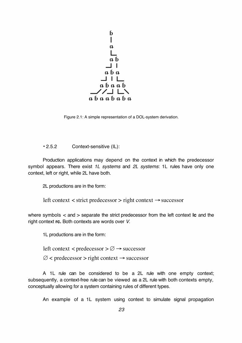
Figure 2.1: A simple representation of a DOL-system derivation.
• 2.5.2 Context-sensitive (IL):
Production applications may depend on the context in which the predecessor symbol appears. There exist 1L systems and 2L systems: 1L rules have only one context, left or right, while 2L have both.
2L productions are in the form:
€
left context < strict predecessor > right context → successor
where symbols < and > separate the strict predecessor from the left context lc and the right context rc. Both contexts are words over V.
1L productions are in the form:
€
left context < predecessor >∅→ successor
€
∅ < predecessor > right context → successor
A 1L rule can be considered to be a 2L rule with one empty context; subsequently, a context-free rule can be viewed as a 2L rule with both contexts empty, conceptually allowing for a system containing rules of different types.
An example of a 1L system using context to simulate signal propagation
23
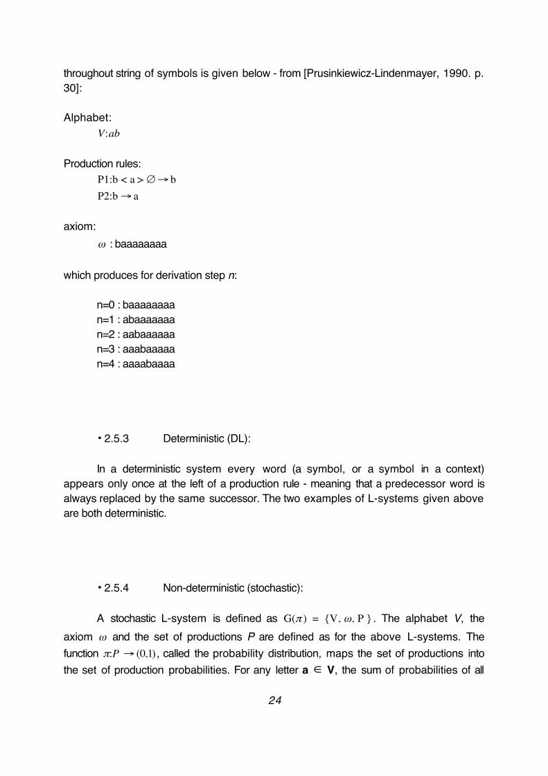
throughout string of symbols is given below - from [Prusinkiewicz-Lindenmayer, 1990. p. 30]:
Alphabet:
€
V:ab
Production rules:
€
P1:b < a > ∅→ b
€
P2:b → a
axiom:
€
ω : baaaaaaaa
which produces for derivation step n:
n=0 : baaaaaaaa n=1 : abaaaaaaa n=2 : aabaaaaaa n=3 : aaabaaaaa n=4 : aaaabaaaa
• 2.5.3 Deterministic (DL):
In a deterministic system every word (a symbol, or a symbol in a context) appears only once at the left of a production rule - meaning that a predecessor word is always replaced by the same successor. The two examples of L-systems given above are both deterministic.
• 2.5.4 Non-deterministic (stochastic):
A stochastic L-system is defined as
€
G(π ) = {V, ω, P } . The alphabet V, the axiom
€
ω and the set of productions P are defined as for the above L-systems. The function
€
π:P → (0,1) , called the probability distribution, maps the set of productions into the set of production probabilities. For any letter a ∈ V, the sum of probabilities of all
24
productions with the same predecessor a is equal to 1. The derivation μ ⇒ ν is called a
stochastic derivation in
€
G(π ) if for each occurrence of the letter a in the word μ the probability of applying production p with the predecessor a is equal to
€
π (p) . Thus, different productions with the same predecessor can be applied to various occurrences of the same letter in one derivation step, causing different outputs.
Non-deterministic rules are in the form:
€
predecessor probability% → successor
where the application of a rule or another on a symbol in the rewriting phase depends on the probability of occurrence assigned to each rule.
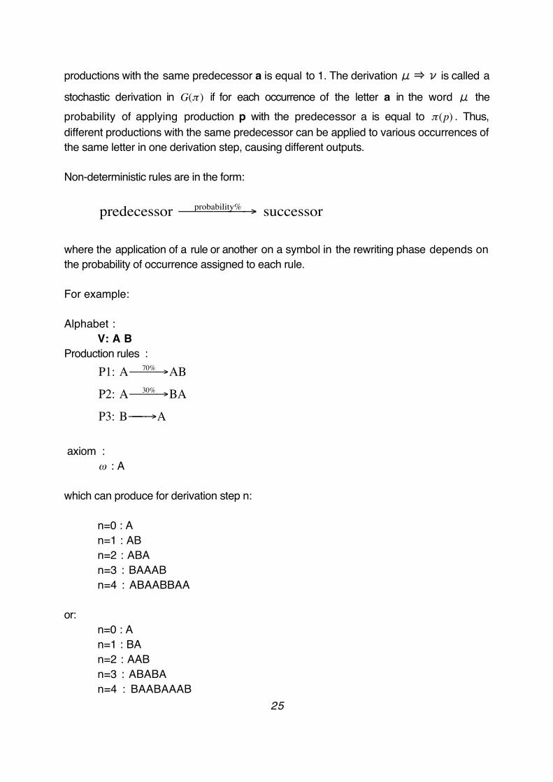
For example:
Alphabet :V: A B
Production rules :
€
P1: A 70% → AB
€
P2: A 30% → BA
€
P3: B → A axiom :
€
ω : A
which can produce for derivation step n:
n=0 : An=1 : ABn=2 : ABAn=3 : BAAABn=4 : ABAABBAA
or:n=0 : An=1 : BAn=2 : AABn=3 : ABABAn=4 : BAABAAAB
25
• 2.5.5 Bracketed L-systems:
The development of the L-system grammars has always been closely related to the models the researchers were trying to simulate. All the examples presented above have a single stream data flow, which could be interpreted as a line, with a beginning, a trajectory and an end. In order to represent axial trees a rewriting mechanism containing branching structures was introduced.
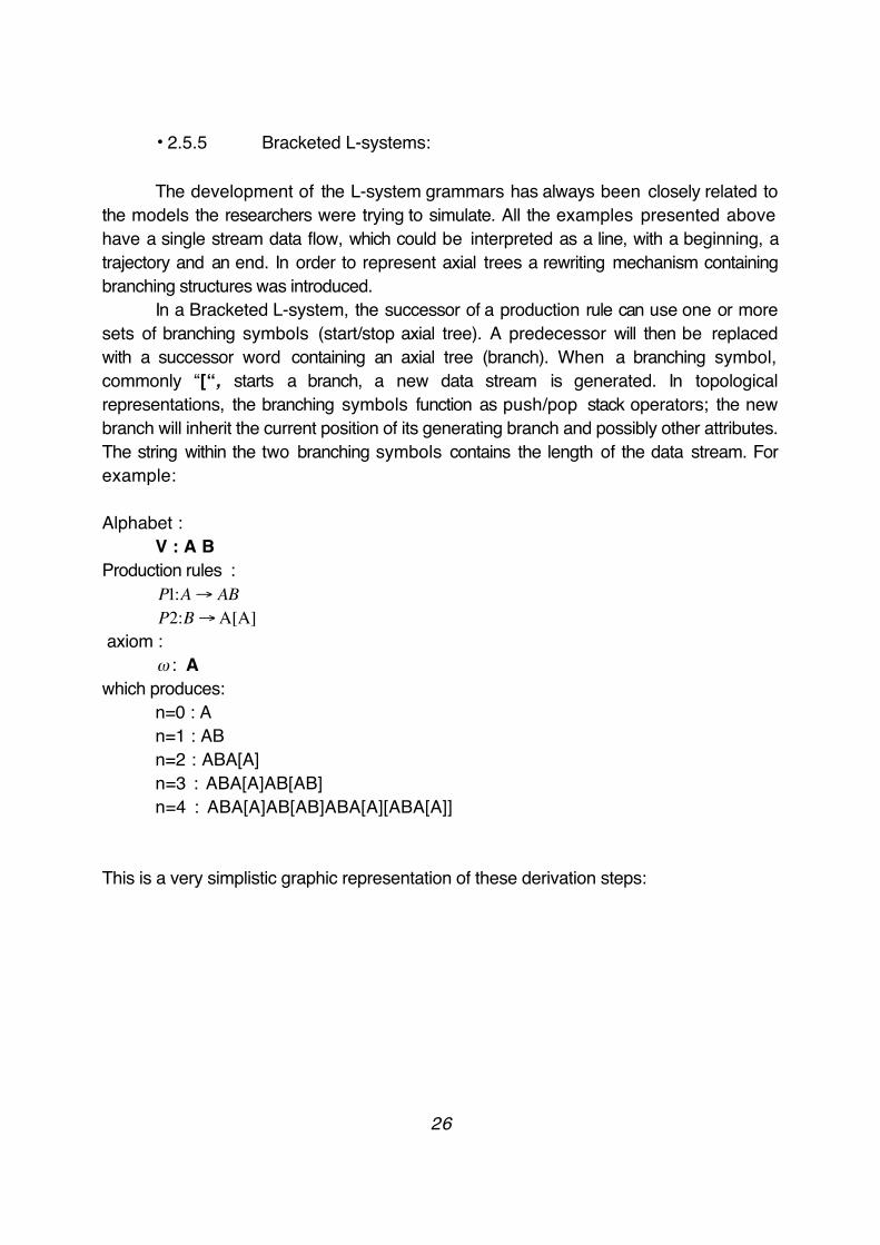
In a Bracketed L-system, the successor of a production rule can use one or more sets of branching symbols (start/stop axial tree). A predecessor will then be replaced with a successor word containing an axial tree (branch). When a branching symbol, commonly “[“, starts a branch, a new data stream is generated. In topological representations, the branching symbols function as push/pop stack operators; the new branch will inherit the current position of its generating branch and possibly other attributes. The string within the two branching symbols contains the length of the data stream. For example:
Alphabet : V : A B
Production rules :
€
P1:A→ AB
€
P2:B→A[A] axiom :
€
ω : Awhich produces:
n=0 : An=1 : AB n=2 : ABA[A] n=3 : ABA[A]AB[AB]n=4 : ABA[A]AB[AB]ABA[A][ABA[A]]
This is a very simplistic graphic representation of these derivation steps:
26
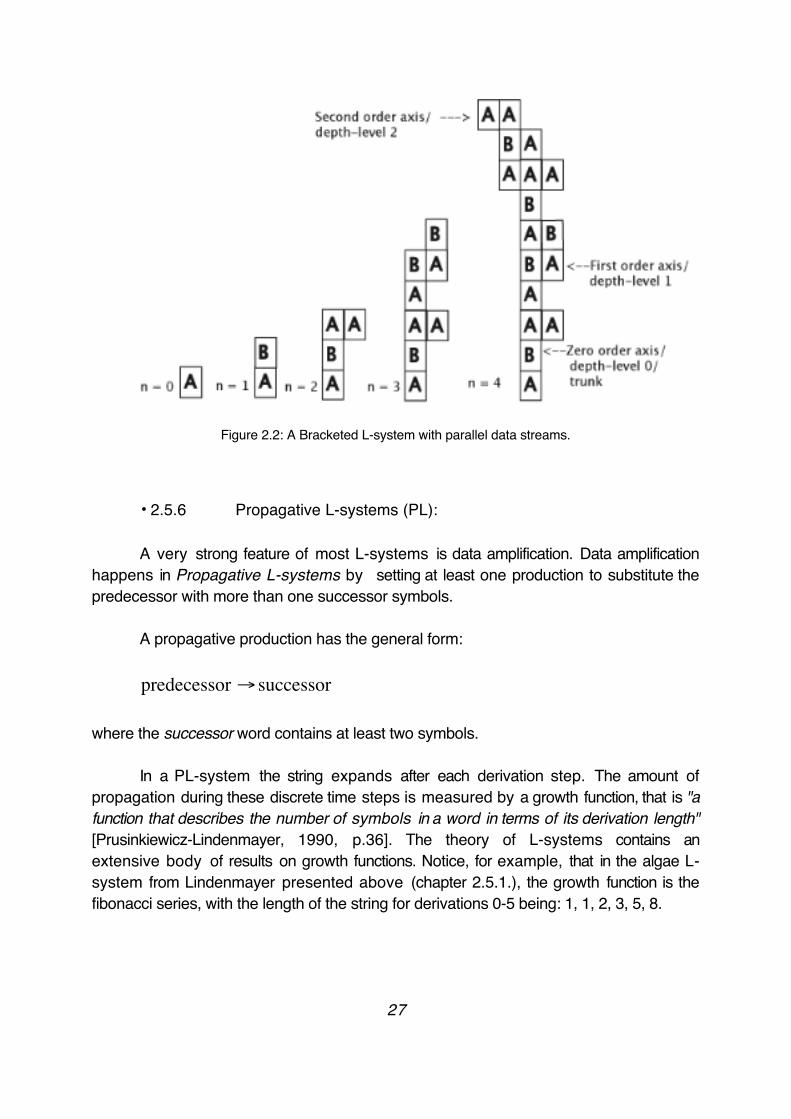
Figure 2.2: A Bracketed L-system with parallel data streams.
• 2.5.6 Propagative L-systems (PL):
A very strong feature of most L-systems is data amplification. Data amplification happens in Propagative L-systems by setting at least one production to substitute the predecessor with more than one successor symbols.
A propagative production has the general form:
€
predecessor → successor
where the successor word contains at least two symbols.
In a PL-system the string expands after each derivation step. The amount of propagation during these discrete time steps is measured by a growth function, that is "a function that describes the number of symbols in a word in terms of its derivation length" [Prusinkiewicz-Lindenmayer, 1990, p.36]. The theory of L-systems contains an extensive body of results on growth functions. Notice, for example, that in the algae L-system from Lindenmayer presented above (chapter 2.5.1.), the growth function is the fibonacci series, with the length of the string for derivations 0-5 being: 1, 1, 2, 3, 5, 8.
27
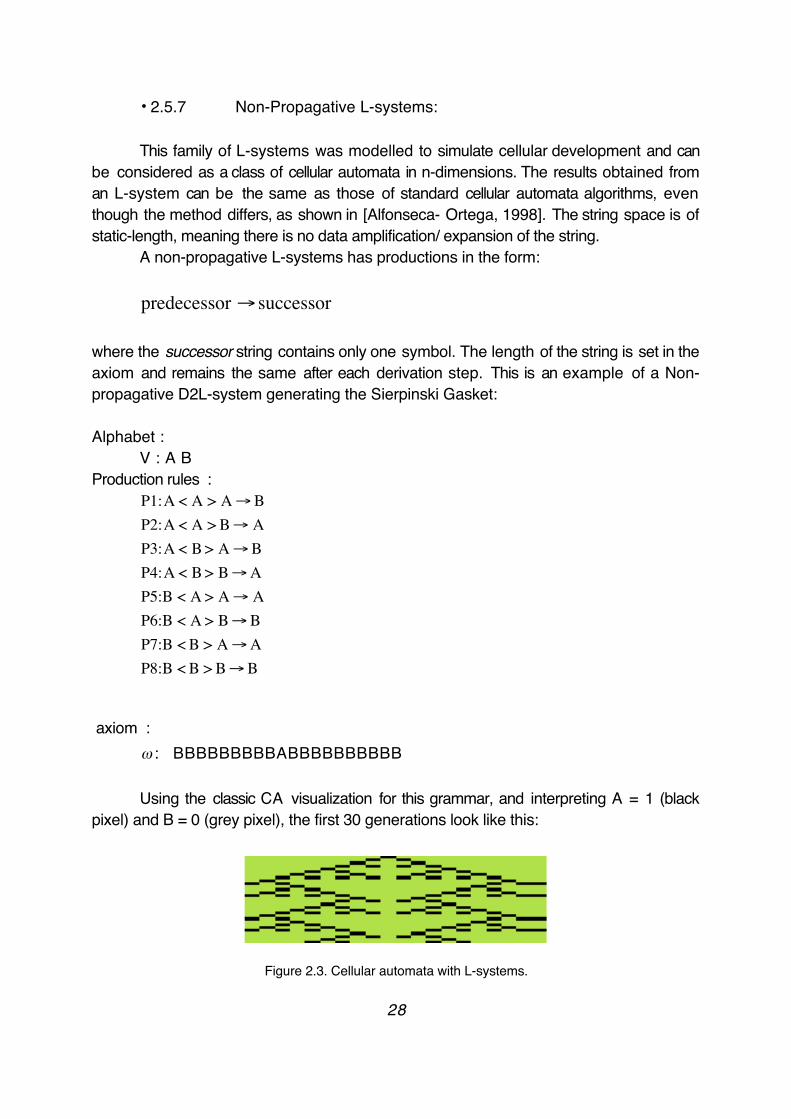
• 2.5.7 Non-Propagative L-systems:
This family of L-systems was modelled to simulate cellular development and can be considered as a class of cellular automata in n-dimensions. The results obtained from an L-system can be the same as those of standard cellular automata algorithms, even though the method differs, as shown in [Alfonseca- Ortega, 1998]. The string space is of static-length, meaning there is no data amplification/ expansion of the string.
A non-propagative L-systems has productions in the form:
€
predecessor → successor
where the successor string contains only one symbol. The length of the string is set in the axiom and remains the same after each derivation step. This is an example of a Non-propagative D2L-system generating the Sierpinski Gasket:
Alphabet : V : A B
Production rules :
€
P1:A < A > A→BP2:A < A > B→ AP3:A < B > A→BP4:A < B > B→AP5:B < A > A→ AP6:B < A > B→BP7:B < B > A→AP8:B < B > B→B
axiom :
€
ω : BBBBBBBBBABBBBBBBBBB
Using the classic CA visualization for this grammar, and interpreting A = 1 (black pixel) and B = 0 (grey pixel), the first 30 generations look like this:
Figure 2.3. Cellular automata with L-systems.
28
• 2.5.8 Table L-systems (TL):
One of the very powerful additions to the initial L-system model was the incorporation of control schemata as a way to program developmental switches in an L-system. This is possible by designing a Table L-system. TL systems were introduced and formalised by Rozenberg in [Herman-Rozenberg, 1975] to simulate the effect of the environment during plant development. They work with different sets of production rules that are called tables. An external control mechanism is used to choose which set of rules will be applied for the current derivation.
An example of a TOL-system is given below:
Alphabet: V: A B
axiom:
€
ω : B
Table 1:Production rules :
€
P1:A→ ABP2:B→ A
Table 2:Production rules :
€
P1:A→ BP2:B→BA
If the set changes on derivation step n=3, this would produce:
T1 n=0 : Bn=1 : An=2 : AB
T2 n=3 : BBAn=4 : BABABn=5 : BABBABBA
29

• 2.5.9 Parametric L-systems:
Parametric L-systems were introduced later in order to compactly deal with situations where irrational numbers need to be used, as well as to provide a meaningful way of internally implementing control mechanisms to model structural change in the system over time. Parametric L-systems make it possible to implement a variant of the technique used for Table L-systems, the difference being that the environment is affecting the model in a quantitative rather than a qualitative manner.
Parametric L-systems operate on parametric words, which are strings of modules consisting of symbols with associated parameters. The symbols belong to an alphabet V, and the parameters belong to the set of real numbers
€
R . A module with letter A ∈ V
and parameters
€
a1,a2...an ∈
€
R is denoted by
€
A(a1,a2 ...an ) . Every module belongs to the set
€
M =V × R∗, where
€
R∗ is the set of all finite sequences of parameters. The set of all strings of modules and the set of all nonempty strings are denoted by
€
M∗ = (V × R∗) ∗ and
€
M+ = (V × R∗) + , respectively.
A parametric OL-system is defined as an ordered quadruplet G = {V, Σ,ω,P}, where• V is the alphabet of the system, • Σ is the set of formal parameters, • ω ∈ (V x∗)+ is a nonempty parametric word called the axiom, • P ⊂ (V xΣ∗) xC(Σ) x(V xE(Σ))∗ is a finite set of productions.
• 2.5.10 L-systems with extension (EL):
Further extensions to the above models of L-systems exist, adding more features to the aforementioned types, with the main focus being on simulating communication between the model and its environment - which acts as a control mechanism upon the L-system. EL-systems include environmentally sensitive L-systems, Open L-systems and Multi-set L-systems.
Environmentally sensitive L-systems work using the same principles as Parametric L-systems, being the next step in the inclusion of environmental factors. The
30
difference between the two types is that in EL-systems the model is affected by the local properties of the environment, rather than global variables. After the interpretation of each derivation step the turtle attributes (see chapter 2.6) are returned as parameters to a reserved query module in the string - the query module being a symbol whose parameters are determined by the state of the turtle in a 3-dimensional space. Syntactically, the query modules have the form: ?X(x,y,z). Depending on the actual symbol X, the values of parameters, x, y and z represent a position or an orientation vector. These parameters can be passed as arguments to user-defined functions, using local properties of the environment at the queried location. Any vector or vectors of the current state can be used.
Environmentally-sensitive L-systems make it possible to control the space in which the model is allowed to grow. In plant modelling they are primarily used to simulate pruning, with the environmental functions defining geometric shapes to which the trees are pruned.
Open L-systems augment the functionality of Environmentally sensitive L-systems. The environment is no longer a function in the system, but is modelled as a parallel system. This represents a shift in the theory, which historically conceived L-systems as closed cybernetic systems, to a more interactive approach, where the model becomes an open cybernetic system, sending information to and receiving information from the environment, (see more in [Mech-Prusinkiewicz, 1996]). Communication modules of the form
€
?E(x1,x2 ...xn ) are used both to send and receive environmental information, represented by the value of the parameters
€
x1, x2...xn . The message is formatted accordingly and shared between the programs modelling the object and the environment.
Multi-set L-systems were introduced “as a framework for local-to-global individual-based models of the spatial distributions of plant communities." [Lane, 2002]. This extension of L-systems allows modelling populations of individual organisms, sharing the same or different rules, which reproduce, interact, and die. "In multiset L-systems, the set of productions operates on a multiset of strings that represent many plants, rather than a single string that represents an individual plant. New strings can be dynamically added to or removed from this multiset, representing organisms that are added to or removed from the population. All interaction between strings is handled through the environment." [Lane, 2002]. A necessary technique for the implementation of Multi-set L-systems is multilevel modelling, which makes it possible to compute and generate the complicated scenes created by the algorithm. Multilevel modelling involves coupling models of a system at successively lower levels of abstraction. The more abstract, higher-level models are created first; the information from them is then used to parameterize the lower-level models.
31
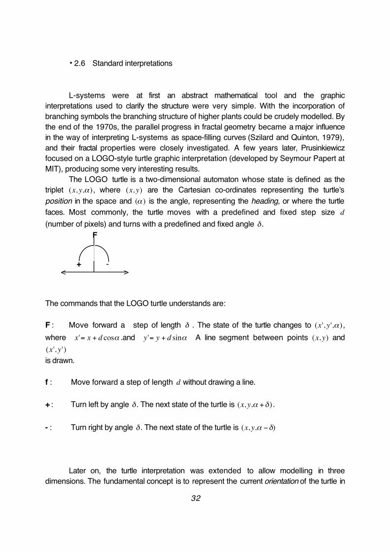
• 2.6 Standard interpretations
L-systems were at first an abstract mathematical tool and the graphic interpretations used to clarify the structure were very simple. With the incorporation of branching symbols the branching structure of higher plants could be crudely modelled. By the end of the 1970s, the parallel progress in fractal geometry became a major influence in the way of interpreting L-systems as space-filling curves (Szilard and Quinton, 1979), and their fractal properties were closely investigated. A few years later, Prusinkiewicz focused on a LOGO-style turtle graphic interpretation (developed by Seymour Papert at MIT), producing some very interesting results.
The LOGO turtle is a two-dimensional automaton whose state is defined as the triplet
€
(x, y,α) , where
€
(x, y) are the Cartesian co-ordinates representing the turtle’s position in the space and
€
(α ) is the angle, representing the heading, or where the turtle faces. Most commonly, the turtle moves with a predefined and fixed step size
€
d (number of pixels) and turns with a predefined and fixed angle
€
δ . F
+ - < >
The commands that the LOGO turtle understands are:
F : Move forward a step of length
€
δ . The state of the turtle changes to
€
(x ', y ',α ) , where
€
x '= x + d cosα .and
€
y '= y + d sinα A line segment between points
€
(x, y) and
€
(x ', y ')is drawn.
f : Move forward a step of length
€
d without drawing a line.
+ : Turn left by angle
€
δ . The next state of the turtle is
€
(x, y,α +δ) .
- : Turn right by angle
€
δ . The next state of the turtle is
€
(x, y,α −δ)
Later on, the turtle interpretation was extended to allow modelling in three dimensions. The fundamental concept is to represent the current orientation of the turtle in
32

a space by three vectors,
€
H,→
L,→
U→
, indicating the turtle‘s heading, the direction to the left, and the direction up. These vectors have unit length, they are perpendicular to each other
and satisfy the equation
€
H ×→
L→
=U→
. The rotations of the turtle are expressed by the equation:
€
H'→
L'→
U'→
= H
→
L→
U→
R
where R is a 3 x 3 rotation matrix. The rotations by angle
€
α about each vector are represented as:
€
RU α( ) =
cosα−sinα
0
sinαcosα
0
001
RL α( ) =
cosα0
sinα
010
−sinα0
cosα
RH α( ) =
100
0cosαsinα
0−sinαcosα
The standard symbols used to control the turtle’ s orientation are :
+ : Turn left by angle
€
δ using rotation matrix
€
RU δ( ) .
- : Turn right by angle
€
δ using rotation matrix
€
RU −δ( ) .
& : Pitch down by angle
€
δ using rotation matrix
€
RL δ( ) .
^ : Pitch up by angle
€
δ using rotation matrix
€
RL −δ( ) .
\ : Roll left by angle
€
δ using rotation matrix
€
RH δ( ) .
/ : Roll right by angle
€
δ using rotation matrix
€
RH −δ( ) .
| : Turn around, using rotation matrix
€
RU 180o( ) .
33
The turtle interpretation of parametric L-systems is essentially the same, except that the step size and rotation angle need not be a global variable but can be declared locally, as a parameter attached to a symbol.
Symbols were first interpreted as simple drawing commands. This model was subsequently expanded, allowing for a symbol to represent a predefined structure/module. The turtle state is used to position that object in the space, while assigned variables may parameterize some of its characteristics.
• 2.7 Current non-standard interpretations
Due to the abstractness of the algorithm and its ability to describe structural development in general, it is increasingly used by researchers for a variety of models, sometimes in combination with genetic algorithms or genetic programming.
In biology, to simulate interactions between the plant and its environment (e.g. plants fighting for water, light and space, insects affecting plants, pruning), as well as to model natural forms in general (plants, shells, mushrooms, animals and animal organs).
In computer graphics, to generate all kinds of scenes, natural or abstract, static or moving. L-systems are currently one of the most powerful image generating methods, as proven by the results, and they are widely used for commercial purposes.
In architecture, to make three-dimensional computer simulations of architectural designs.
In artificial life models, were the ‘mind’ or behavior of an agent can be coded into a set of rules which allow interaction with the environment or other agents, while its ‘body’ or graphic appearance can be represented and designed generatively - using the L-system as the AI ‘s DNA.
In neural network research L-systems are used to set up and develop the structure of the network.
In linguistics, they are used to model the development of linguistic structures through language acquisition and the structural interpolation from the semantic concept that lies behind the deep structure of an utterance to its surface structure.
In robotics, to find and create the proper structure for connecting a number of two-dimensional or three-dimensional modular robots in a way that allows them to move naturally as a unit.
In data compression, to detect structural periodicities in the input and turn them into production rules, compressing the input into a deterministic formal grammar which can subsequently be used to regenerate the input.
Finally, L-systems are also used in music. The musical applications will be discussed in the following chapter.
34

▼ Chapter 3: The connection to music.
3.1. L-system music: Previous implementations.
Up to now, there has been a fairly limited number of implementations using L-systems for generating musical data. Having as a fundamental idea the interpretation proposed by Przemyslaw Prusinkiewicz [Prusinkiewicz, 1986] they are all active on the note level.
In this paper, Prusinkiewicz proposes an interpretation system that works by performing a spatial mapping of the L-system output, using an approach related to [Dodge & Bahn, 1986] and [Voss & Clarke, 1978]. The L-system output string is first drawn as a 2-dimensional graph using a turtle interpreter; the resulting geometric shape is then traced in the order in which it was drawn. In Prusinkiewicz's words, "the proposed musical interpretation of L-systems is closely related to their graphic interpretation, which in turn associates L-systems to fractals." The different dimensions of the shape are mapped to musical parameters, such as pitch height for y and duration for x, though Prusinkiewicz suggests that other parameters, like velocity and tempo, could be controlled as well. A fixed grid is used for both vectors: a musical scale defined as MIDI values for pitch and a fixed metric value for duration. As such, each forward movement of the turtle pen along the x-axis represents a new note of a fixed metric duration, with multiple forward movements in the same direction (with no intervening turns) represented as notes of longer duration.
However trivial this type of mapping might seem, Prusinkiewicz makes two very interesting suggestions. The first is the spatial mapping of the output. Despite the objections one might have to the concrete application - due to the unnecessary subordination of the musical data to the visual data and the binding of the interpretation to a traditional musical concept - the abstract model is conceptually intriguing, since L-systems are very powerful in spatial representations. Thus, the basic idea from Prusinkiewicz to take and develop further is that the algorithm generates a fractal trajectory which the composer can map to a desired parameter space. The act of designing this space and its resolution - or perceptual grid - is in itself a major part of the compositional procedure.
Another important concept is that of branching as polyphony. Diverging again from the MIDI note paradigm, the output of a branched L-system can be used as a hierarchical, self-similar, contrapuntal data structure with multiple voices and varying overall density.
35
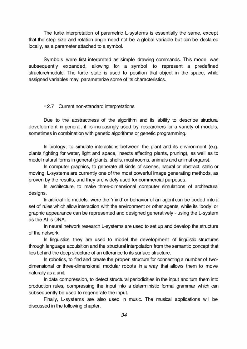
The system Prusinkiewicz proposes would look like this:
Figure 3.1 Prusinkiewicz’ s L-system interpreter concept.
Following an increasing trend towards using fractal algorithms and grammars in that period, Prusinkiewicz's article had some impact on composers who were already familiar with such models.
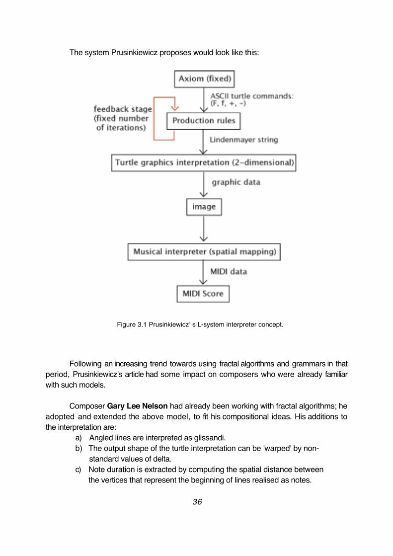
Composer Gary Lee Nelson had already been working with fractal algorithms; he adopted and extended the above model, to fit his compositional ideas. His additions to the interpretation are:
a) Angled lines are interpreted as glissandi. b) The output shape of the turtle interpretation can be 'warped' by non-
standard values of delta.c) Note duration is extracted by computing the spatial distance between
the vertices that represent the beginning of lines realised as notes.
36
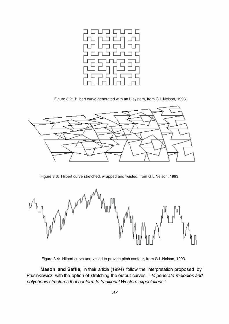
Figure 3.2: Hilbert curve generated with an L-system, from G.L.Nelson, 1993.
Figure 3.3: Hilbert curve stretched, wrapped and twisted, from G.L.Nelson, 1993.
Figure 3.4: Hilbert curve unravelled to provide pitch contour, from G.L.Nelson, 1993.
Mason and Saffle, in their article (1994) follow the interpretation proposed by Prusinkiewicz, with the option of stretching the output curves, " to generate melodies and polyphonic structures that conform to traditional Western expectations."
37
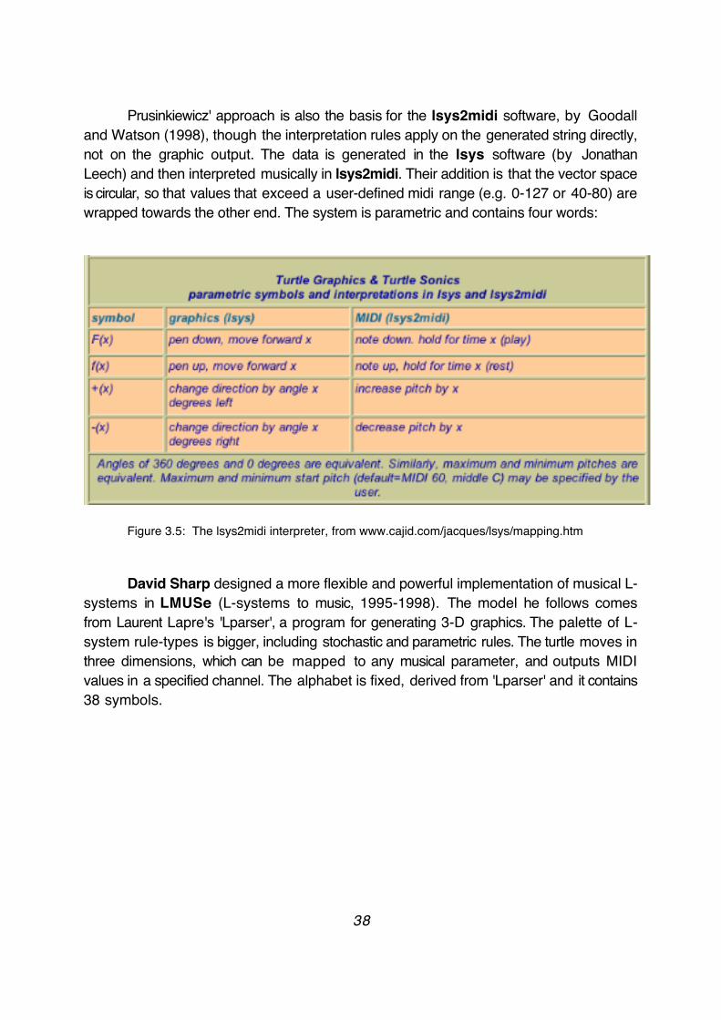
Prusinkiewicz' approach is also the basis for the lsys2midi software, by Goodall and Watson (1998), though the interpretation rules apply on the generated string directly, not on the graphic output. The data is generated in the lsys software (by Jonathan Leech) and then interpreted musically in lsys2midi. Their addition is that the vector space is circular, so that values that exceed a user-defined midi range (e.g. 0-127 or 40-80) are wrapped towards the other end. The system is parametric and contains four words:
Figure 3.5: The lsys2midi interpreter, from www.cajid.com/jacques/lsys/mapping.htm
David Sharp designed a more flexible and powerful implementation of musical L-systems in LMUSe (L-systems to music, 1995-1998). The model he follows comes from Laurent Lapre's 'Lparser', a program for generating 3-D graphics. The palette of L-system rule-types is bigger, including stochastic and parametric rules. The turtle moves in three dimensions, which can be mapped to any musical parameter, and outputs MIDI values in a specified channel. The alphabet is fixed, derived from 'Lparser' and it contains 38 symbols.
38
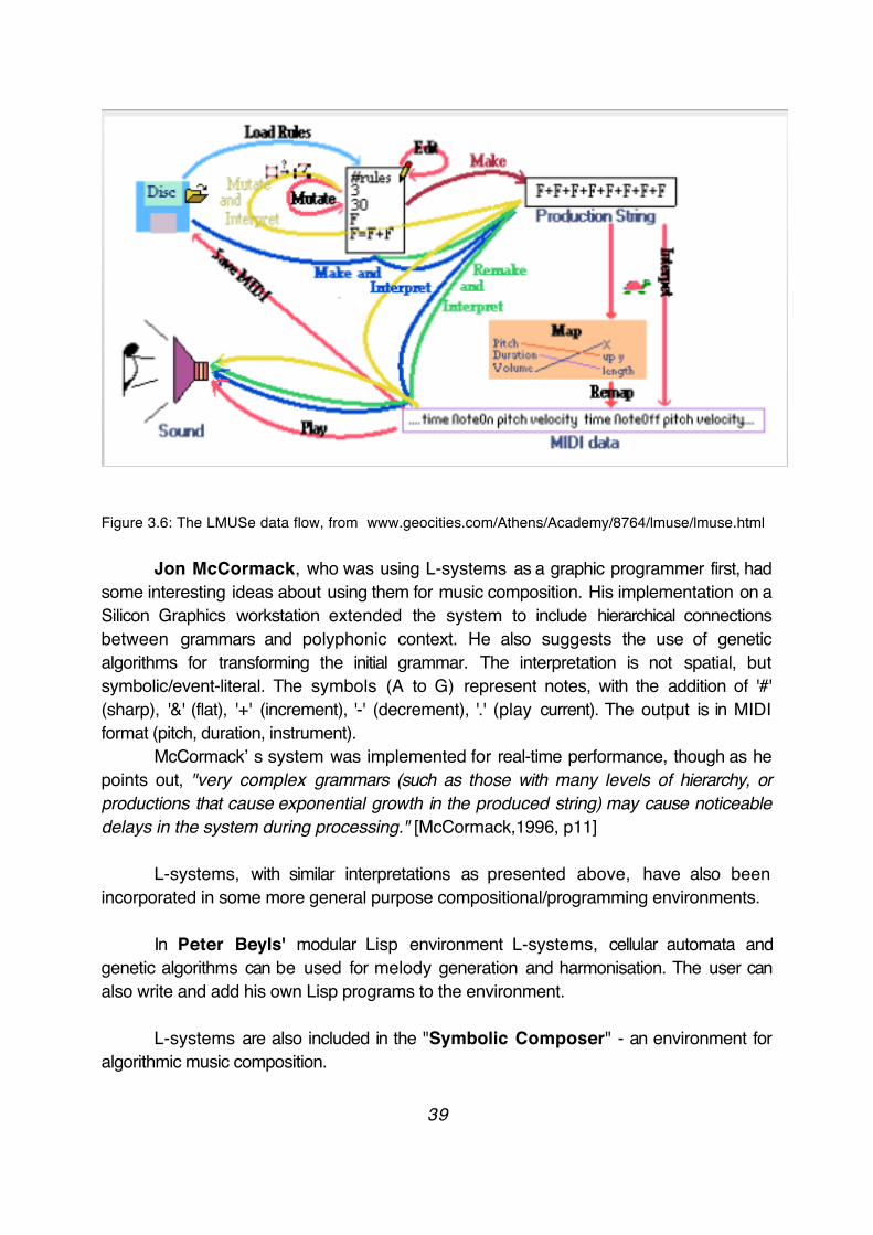
Figure 3.6: The LMUSe data flow, from www.geocities.com/Athens/Academy/8764/lmuse/lmuse.html
Jon McCormack, who was using L-systems as a graphic programmer first, had some interesting ideas about using them for music composition. His implementation on a Silicon Graphics workstation extended the system to include hierarchical connections between grammars and polyphonic context. He also suggests the use of genetic algorithms for transforming the initial grammar. The interpretation is not spatial, but symbolic/event-literal. The symbols (A to G) represent notes, with the addition of '#' (sharp), '&' (flat), '+' (increment), '-' (decrement), '.' (play current). The output is in MIDI format (pitch, duration, instrument).
McCormack’ s system was implemented for real-time performance, though as he points out, "very complex grammars (such as those with many levels of hierarchy, or productions that cause exponential growth in the produced string) may cause noticeable delays in the system during processing." [McCormack,1996, p11]
L-systems, with similar interpretations as presented above, have also been incorporated in some more general purpose compositional/programming environments.
In Peter Beyls' modular Lisp environment L-systems, cellular automata and genetic algorithms can be used for melody generation and harmonisation. The user can also write and add his own Lisp programs to the environment.
L-systems are also included in the "Symbolic Composer" - an environment for algorithmic music composition.
39

Michael Gogins focuses on the topological attributes of L-systems in Silence, a Java program using his Music Modelling Language. The environment is in itself hierarchical, with ‘Definition’ and ‘Use’ nodes. L-systems can be used as an algorithm for navigating in the musical space, which has eleven linear and unconnected dimensions.
Luke Dubois built 'jit.linden’, an object implementing L-systems for the Jitter programming environment. The object is now part of the original Jitter distribution. In his thesis "Applications of Generative String-Substitution Systems in Computer Music" he also implements static-length L-systems (1-dimensional cellular automata) and produces some interesting ideas about timing and interactive performance using L-systems.
Figure 3.7: Data flow of DuBois’ system, from [DuBois, 2003].
40
The input from a performer is analysed, categorised and coded into symbols. These symbols are then treated as the axiom for an L-system. The data produced are used for visual and sonic accompaniment, with turtle-like graphics and delays performing pitch shifting on the input signal. A score follower is used to make adjustments to the interpretation rules according to a predefined compositional plan.
DuBois is particularly interested in making a closely related visualisation and sonification of the L-system output, which stresses the focus more on the algorithm than on the music; his goal is "to generate algorithmic music that explores the features of the algorithm used in a vivid and interesting way." [DuBois, 2003]
• 3.1.1 Assessment of the previous implementations.
"A new poetry is only possible with a new grammar." [Roads, 1978, p. 53]
The development of L-systems has always been related to the model they are called to represent. The algorithm, from the production to the interpretation and mapping, has to be designed and 'tuned' according to the desired result - a process frequently involving heuristics - and the validity of the model is judged by the result. In the case of organic growth 'simulations', which is what most of the corpus on L-systems deals with, a system has to solve a growth problem and generate a graphic object of the solution in the most credible and naturally looking way. A simulation, however, can also be dealing with an abstraction or the non-real [Hornby-Pollack, 2002]; the concepts of 'credible' and 'natural looking' then need to be redefined according to the goal and reshaped according to the medium.
This should be obvious for every implementation of L-systems that takes place in a field other than computer graphics. It is rarely true, though, for the above musical implementations. Most commonly, and this dates from Prusinkiewicz 's first suggestions, the goal seems to be simulating the simulation. This is reflected both when the graphic output of an L-system is interpreted musically, as well as when known and investigated rules coming from other fields, mainly computer graphics, are used to generate music. Less frequently, the model is properly adjusted to the music medium. In those cases, however, the simulation is forced to be 'natural', tied to the misconception that the western tonal system is an equivalent to the physical laws in music. Thus, the focus is shifted from
41

music either to sonification or to musicology.
The focus of this thesis is neither the former nor the latter. The reason for using L-systems is to make purely musical structures. This is reflected in all the levels of the algorithm when a musical L- system is being designed. Music is an art, and the notions of 'credible' or 'natural looking' are defined differently for artistic and scientific 'simulations', even though the tools may be the same. The fundamental difference is that there is no objective likeliness forced by an external semantic system (the real world) but subjective opinion and compositional tactics. The only physical law analogy is the aesthetics of the composer judging the sonic output of the system he designed. The strategy for making a musical L-system should, thus, be radically unique, fitting the method to the music while underlying its properties, and not vice versa. Or, as C. Roads wisely suggests, "ultimately, the question is not whether music conforms to the structure of formal grammars, but rather whether particular formal grammars can be designed, which are useful representations of certain compositions." [Roads, 1978, p. 53].
Moreover, the technical and conceptual limitation of interpreting the output of an L-system as 7-bit MIDI values needs to be overcome. Technically, complex dynamic structures as those that can be generated by L-systems cannot be expressed properly within such a limited bandwidth of an integer space. This extreme quantization of the turtle's trajectory in the phase space - phase space being the space in which all possible states of the system are represented - will distort the output, leading to forced periodicities. For the same reason that a graphic interpretation of a tree model would never be accurate in a 128x128 pixel resolution, a MIDI-like treatment should be excluded. Apart from this extreme quantization, the score paradigm which was proposed by Prusinkiewicz and followed by all the other implementations - even when other options would be possible - is also conceptually limiting and inadequate for any but traditional music. Contemporary instrumental music has rejected this two-dimensional model as well, in the need to expand the compositional space. When such a concept is applied to electronic music it is simply out of context.
Quantization and discreteness thus have to be replaced with perceptual continuity. Euclidean arithmetics has to give its place to floating-point arithmetics as “a rational approximation of operations on real, in the mathematical sense, numbers" [Wishart, 1994, p. 108], making the progression from the rational to the real possible, in both the mathematical and the musical sense. The Cartesian space has to expand to a multi-dimensional one, capable of controlling "the multi-dimensional complexity of the sound world" [Wishart, 1994, p. 104].
42

3.2. In the quest for the right abstraction.
A certain degree of formalism has always been a basis for Western music. In the 20th century, the expansion of the compositional space of music and the tendency towards designing increasingly more complex structures augmented the shift towards more abstract models of composition. The scope of composing radically changed with the introduction of digital computers. Digitalization brought an enormous field of sciences and arts together, sharing the same tools and communicating with the same language. Science and technology provided composers the means for organizing procedures and formalisms in a higher level, shifting their attention from the details to the overall strategy. The electronic music composer is now a musician, a philosopher and a multi-scientist, in the quest for the right abstraction that will allow him to use and master the quasi-infinite possibilities technology can offer him to make music.
One could say that the power of digital technology resides in the fact that it allows us to make complex simulations and gain insight on various aspects of the world and of the imagination. A simulation can be defined as an imitation of a process or of a system and it presupposes the acquisition of valid information about the referent. The act of simulating in general requires representing certain key characteristics or behaviours of a natural or abstract system in a compact and simplest possible way. The success of a simulation is judged by the fidelity and validity of the outcome, and the flexibility of the model in explaining the general properties of the referent.
The continuous intrusion of rationality into what used to be inexplicable has expanded human understanding to the previously unknown and unthought of. Similarly, the ideas we have about music, and our methodologies in composing have undertaken a constant and continuous permutation. This is clearly reflected in Xenakis' s words: '"Freed from tedious calculations the composer is able to devote himself to the general problems that the new musical form poses and to explore the nooks and crannies of this form while modifying the values of the input data.(...) With the aid of electronic computers the composer becomes sort of a pilot: he presses the buttons, introduces co-ordinates, and supervises the controls of a cosmic vessel sailing in the space of sound, across sonic constellations and galaxies that he could formerly glimpse only as a distant dream. Now he can explore them at his ease, sitting in an armchair." [Xenakis, 1992, p.144]. The advent of computers gave us the possibility to formulate, abstract and simulate 'natural' and 'synthetic' environments in radically novel manners. The quest for abstract modelling and organization of complex musical behaviours has manifested itself in the various algorithmic procedures that have been broadly used throughout the history of electronic music.
Music is a complex system with structure and development in time, demanding careful and concise planning and organization of the compositional procedure. The
43

fundamental assumption for using an algorithm to model a musical process is that logic and mathematics can provide a useful abstraction for such a task. The recent studies in complex dynamic systems, permitted by the advancement in CPU power, can be a very fruitful metaphor. Indeed, music can be thought of as a complex dynamic system with dynamic structure, permitting us to follow a similar methodology in order to generate a musical behavior. Prusinkiewicz comments: "Many natural phenomena can be modelled as dynamical systems. At any point in time, a dynamical system is characterised by its state. A state is represented by a set of state variables. (...)Changes of the state over time are described by a transition function, which determines the next state of the system as a function of its previous state and, possibly, the values of external variables (input to the system). This progression of states forms a trajectory of the system in its phase space (the set of all possible states of the system)." [Prusinkiewicz, 2003, p 1-2]
In order to generate any complex process, the system to be modelled must be divided into a set of components, separating the system from its field of activity. In the case of a musical system, the basic components are:
1) the parameter space.2) the grid for each vector in the space.3) the movement in time in the space.As such, the phase space of this system is the n-dimensional compositional
parameter space with its grids/ reference frames for every vector and its trajectory is represented by the movement of the state variables for every vector in time. The current state of the system is represented by the set of the states for every vector.
The concept of describing a musical system trajectory through a phase space could be expanded to include hierarchical structures - a fundamental characteristic of music - further decomposing the modelled system into a set of functional components. These hierarchies can be time level hierarchies and/or parameter hierarchies. In the first case, we can think of the musical system as a tree structure with embedded time scale components (macro, meso, etc.). In the second case, we can think of the phase space of music as the perceptual phase space of sound with each of its dimensions containing embedded spaces with their vectors corresponding to the instrument parameters that have the most effect in the respective perceptual dimension. In both cases, a change in any of the system ‘s components will affect the system in total, depending on the components structural function. "Many dynamical systems can be decomposed into parts. The advancement of the state of the whole system is then viewed as the result of the advancement of the state of its components. (...) Formally, we use the term structured dynamical system to denote a dynamical system divided into component subsystems (units)." [Prusinkiewicz, 2003, p 1-3].
Having found a formalism for modelling a complex structured behavior, the following step is to look for a way to incorporate the appropriate control schemata for dynamically organizing development in time. The metaphor comes again from biology: "A developing multicellular organism can be viewed as a dynamical system in which not
44
only the values of state variables, but also the set of state variables and the state transition function change over time. These phenomena can be captured using an extension of structured dynamic systems, in which the set of subsystems or the topology of their connections may dynamically change. We call these systems dynamical systems with a dynamic structure ." [Prusinkiewicz, 2003, p 1-3]. Or, interpreting the above statement musically, a musical system can be viewed as a dynamic system in which not only the values of the state in the parameter space, but also the mapping (and the grids) of the parameter space and the rules change over time.
Lindenmayer systems provide a very compact and efficient formalism for designing a musical system. Quoting Prusinkiewicz again, "L-system models are inherently dynamic, which means that the form of an organism is viewed as a result of development: 'an event in spacetime, and not merely a configuration in space' (D' Arcy Thompson)" [Prusinkiewicz, 2003, p 1-4]. L-systems are used as a formal model for focusing on the computational (algorithmic) aspects of pattern formation processes, and not in the patterns themselves. This makes it possible to recognize and analyse similarities between apparently different realizations of similar patterns, and to follow their process of formation in time. The main goal of L-systems has been to model structure and form as a result of development, emphasizing on the functional relations that hold between the different parts of a system, rather than the parts themselves. "Thus, a particular form is modelled by capturing the essence of the developmental process that leads to this form." [Prusinkiewicz-Lindenmayer, 1990, p.63]. These relations include the transfer of information, and circular relations (feedback) that result in emergent phenomena. The concepts of emergence and morphogenesis - central themes in electronic music for the past few decades -are fundamental to L-systems.
3.3. Form and navigation: L-systems as grammars and fractals.
The concept of rules in music has been common grounds for a very long time. Various types of analytical 'grammars' have been proposed to explain musical behaviours. The rules of these grammars are usually in the form of constraints and restrictions, regulating the pathways one can take in the musical space. Schenkerian analysis is a form of recursive hierarchical grammar, active in three time-levels of a musical composition, the foreground, the middleground and the background. The success of linguistic formalisms during the second part of the 20th century in explaining aspects of complex language systems has had an important influence on musical thought. This belief in the power of grammatical representational models is clearly reflected in Curtis Roads' following optimistic statement: "There is a very broad range of music which can be described naturally using grammars. Any music which can be partitioned can be
45

described by a grammar." [Roads, 1979, p. 49]. The influence of the theories of Chomsky and Schenker can be clearly traced in the work of Lerdahl and Jackendoff. Their theory on ‘the capacity for music’ is an expansion of Chomskyan thought to the field of music. Their proposition is that in a musical idiom there are well-formedness and preference rules; the first kind of rules generates a set of possible interpretations of a structure, while the second will choose to acknowledge this or the other rule option as a valid interpretation. This is a form of a 'regulated grammar', that is, a formal grammar with a super-ordinate control mechanism. Their focus is on time level hierarchies and their interaction. Several researchers have used linguistic related approaches to explain musical structure and meaning, including L. Bernstein, Ruwet, Nattiez, Laske, Smoliar.
However, analysis of given musical structures is not the only field where a musical grammar can be implemented. Hierarchies and transformations can be used in the structural formation of any musical idiom - traditional or novel. Indeed, Roads suggests that "the range of possible grammars is quite broad and their expressive scope is very extensive; thus there is no intrinsic reason why grammars should only be useful for representing traditional music". [Roads, 1978, p. 53]. A compositional process can be regarded as the application of a set of strategies or rules that will translate the concept that the composer has for the deep structure to the actual sonic output. For G.M. Koenig this is clear: "By composition processes do we mean the composition of musical language structures? Emphatically, yes. Composing terminates in pieces, and the extent to which pieces are put together from sounds, and the relations prevailing among these sounds, are a matter of how a composer works. Composition is the application of a grammar which generates the structures of a piece, whether the composer is aware of an explicit grammar or not" [Koenig, 1978, p. 2]. For electronic music in particular, the language metaphor is a very valid one, since the fundamentals of computer languages are based exactly on the formalisms proposed by linguists like Chomsky. As such, grammar models can be used not only as an analysis method but also as a generative one. Several composers have implemented generative grammars for computer music, including J.A. Moorer, C. Roads, W. Buxton, S.R. Holtzman, M. Gogins, S. T. Pope.
An L-system is a semantically agnostic symbolic structure that develops in time. Its semantic relation to the modelled structure is not iconic but symbolic, meaning that there is no topological similarity or contiguity between the sign and the signifier, but only a conventional arbitrary link. The production side of the algorithm is decoupled from the interpretation side and the mapping, allowing the composer to flexibly use the algorithm according to the plan of a musical piece. This separation is very important for turning any type of formal grammar into a valid model for musical data generation. Curtis Roads notes on the subject: "Maximum flexibility is achieved by logically separating the syntactic specification (...) from the sonic specification." [Roads, 1979, p. 53]. The symbols of the alphabet can be interpreted in any desirable way - that is the reason why L-systems can be successfully used in such a variety of fields besides biology. In the same system various kinds of mappings may be used in order to model a musical structure.
46
Interpretation can be abstract or concrete, a symbol may be mapped to a specific action or it may be used as a hierarchical node that incorporates a number of other actions/ structures, or as a control schema for the environment or the L-system itself. This makes Lindenmayer systems a powerful algorithm for modelling musical structures.
Initially, L-systems were conceived as an abstract mathematical formalism where the symbols represent a functional unit in the structure of the modelled system. Later on, with the incorporation of graphic interpretations, their use expanded into generating space-filling curves with self-similar fractal structures. According to Manfred Schroeder, "the unifying concept underlying fractals, chaos and power laws is self-similarity. Self-similarity, or invariance against changes in scale or size, is an attribute of many laws of nature and innumerable phenomena in the world around us. Self-similarity is, in fact, one of the decisive symmetries that shape our universe and our efforts to comprehend it." [Schroeder, 1991, p. xii]. In 1978, Voss and Clarke published the article "1/f noise in music: Music from 1/f noise", where they claimed that the temporal aspects of various kinds of music - rhythmical and formal structures, as well as instantaneous pitch - are self-similar with a 1/f noise distribution. In addition, listeners judged 1/f distributions the most musical - 1/f0 was too random and 1/f2 was too correlated. Mandelbrot defined self-similar structures as follows: "When each piece of a shape is geometrically similar to the whole, both the shape and the cascade that generate it are called self-similar." [Mandelbrot, 1982, p. 34]. Another basic property of fractals is the appearance of 'strange attractors,' meaning numbers in the system that tend to exert a particular pull on the field around them. These properties of fractal algorithms have attracted a number of composers to use them as real-time or non-real time musical data generators, such as Charles Dodge, G.L. Nelson, J.C.Risset, M. McNabb, Ch. Wuorinen, Sh. D. Yadegari. In general, fractals have been used either to model embedded musical structures (Dodge, Profile), or to generate trajectories in a parameter space (usually melodies), or even to generate waveforms in the sample level by mid-point subdivision [Yadegari, 1991, 1992].
Despite their apparent capability of generating interesting spatial trajectories, fractal algorithms have an inherent problem of timing and of developing over time. "I think one reason mathematically-based algorithms overproduce ill-formed pieces is that such algorithm operate ' outside of time'. By this, I mean that the space in which the algorithms operate is typically a simple Euclidian space(...) Another obstacle is that (...) pitch as a dimension of music does not seem to be isomorphic to time as another dimension of music". [Gogins, 2005, pp. 1-2]. The following remark from Ben Goertzel on melodies could be expanded to any musical vector: "Fractal melodies are structured on many different scales. Admittedly, however, there are differences between this fractal structure and what we ordinarily think of as musical structure. The most important difference is the sense of progressive development over time - most human music has this, but very little fractal music does. The most interesting fractal melodies are those which,
47
coincidentally, do happen to display progressive development." [Goertzel, 1997]. As such, a musical fractal algorithm would benefit from its subordination to a control structure, allowing the composer to make a plan of development of the algorithm over time. Control mechanisms are incorporated in L-systems and can be endogenous (1), defined in the system, and exogenous, coming from the environment. The musical system can, thus, be modelled as a closed or open cybernetic system, respectively.
Summarizing, some of the most useful features of L-systems for making music are: symbolic representation/abstractness and data amplification/compactness, parallel substitution of all the symbols in the string, the ability to design hierarchical connections - in the system with Bracketed L-systems and with multiple systems with Hierarchical L-systems - self-similarity of the output, spatial representations, incorporation of control schemata.
In the application presented in the following chapter the focus has been in providing a flexible and open framework for exploring the different possibilities for composing with L-systems. The implementation of different grammar types, interpretations and mappings will be presented, as well as that of control mechanisms for transforming the rules of the L-systems over time. Finally, I will consider some specific ideas and compositional strategies for every time level of music and include audio examples.
(1). With lineage or interaction: "The term lineage (or cellular descent) refers to the transfer of information from an ancestor cell or module to its descendants. (OL-systems) In contrast, interaction is the mechanism of information exchange between neighbouring cells (IL-systems)" [Prusinkiewicz-Lindenmayer, 1990, p.65]
48
“The forms of living organisms are the result of continuous process of flow (growth) - they are morphic forms captured in space. Even the calcified remains of sea creatures (...) tell us about the processes of continuous growth which formed them, and any spatial proportions we may observe in the final forms are merely the traces of these continuous processes, time-flows revealed in space.
What strikes us as formally coherent about a tree is not some exact and static proportioning of branching points and branch angles, but the way in which a flexible (and environmentally sensitive) expression of some branching principle is realised through a process of branching flow. The overall state of a particular flow pattern (its result being the current state of the tree) links our perception of one member of a tree species with the other members of the same species.
Unlike the growing tree, a musical event never fixes its time-flow evolution in a spatial object, it is intrinsically evanescent and a musical score is not the musical experience itself, but a set of instruction to generate this aetherial experience, just as the genetic code is a set of instructions to grow an organism.”
[Trevor Wishart, Audible design, p. 110]
▼ Chapter4: My implementations.
• 4.1 The compositional environment:
My implementation is realized in the Max/MSP/Jitter programming environment. The L-system algorithm has been incorporated in a real-time compositional surface that I have built. The approach is modular, based on a modified version of the open-source lloopp server (1). The main modifications have been to develop a version which supports list and matrix operations. This was necessary in order to expand the already existing structure from the classic ‘hands-on’ live performance/ improvisation paradigm to
(1): The original lloopp server, built by Klaus Filip, can be found at www.lloopp.klingt.org49
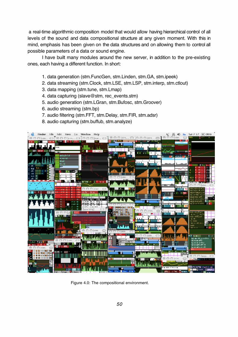
a real-time algorithmic composition model that would allow having hierarchical control of all levels of the sound and data compositional structure at any given moment. With this in mind, emphasis has been given on the data structures and on allowing them to control all possible parameters of a data or sound engine.
I have built many modules around the new server, in addition to the pre-existing ones, each having a different function. In short:
1. data generation (stm.FuncGen, stm.Linden, stm.GA, stm.ipeek)2. data streaming (stm.Clock, stm.LSE, stm.LSP, stm.interp, stm.ctlout)3. data mapping (stm.tune, stm.Lmap)4. data capturing (slave@stm, rec_events.stm)5. audio generation (stm.LGran, stm.Bufosc, stm.Groover)6. audio streaming (stm.bp)7. audio filtering (stm.FFT, stm.Delay, stm.FIR, stm.adsr)8. audio capturing (stm.buffub, stm.analyze)
Figure 4.0: The compositional environment.
50
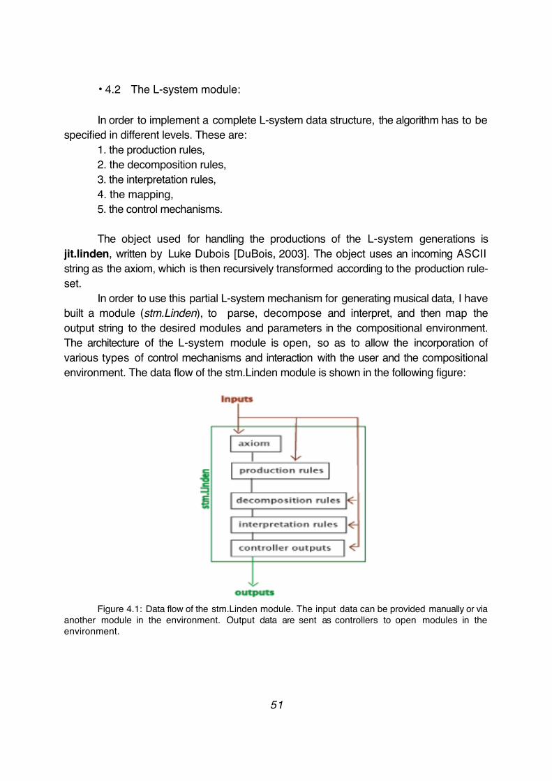
• 4.2 The L-system module:
In order to implement a complete L-system data structure, the algorithm has to be specified in different levels. These are:
1. the production rules, 2. the decomposition rules,3. the interpretation rules,4. the mapping,5. the control mechanisms.
The object used for handling the productions of the L-system generations is jit.linden, written by Luke Dubois [DuBois, 2003]. The object uses an incoming ASCII string as the axiom, which is then recursively transformed according to the production rule-set.
In order to use this partial L-system mechanism for generating musical data, I have built a module (stm.Linden), to parse, decompose and interpret, and then map the output string to the desired modules and parameters in the compositional environment. The architecture of the L-system module is open, so as to allow the incorporation of various types of control mechanisms and interaction with the user and the compositional environment. The data flow of the stm.Linden module is shown in the following figure:
Figure 4.1: Data flow of the stm.Linden module. The input data can be provided manually or via another module in the environment. Output data are sent as controllers to open modules in the environment.
51

In the application presented in this thesis, I have implemented the following types of L-systems for designing musical structures in all the time levels of a composition:- Deterministic L-systems.- Context-free L-systems.- Context-sensitive L-systems (1L and 2L).- Propagative and Non Propagative L-systems.- Table L-systems.- L-systems with extensions:
Environmentally sensitive extensions.Parametric extensions.Stochastic extensions.Evolving grammars.Hierarchical L-systems.Multi-set L-systems.Interactive (Open) L-systems.
Due to certain limitations of the jit.linden object, in this implementation I tried to focus on the different possible interpretations, mappings and control mechanism that can be valid for a musical L-system - more attention is, thus, given not on the production side of the algorithm, but on the musical potential of its output. The limitations of the object, when compared to the actual model used for graphics and described in [Prusinkiewicz-Lindenmayer, 1990], [Prusinkiewicz-Hannan-Mech, 1999], [Karwowski-Prusinkiewicz, 2003], are the following:
-The production rules are deterministic. Stochastic functions can only be used while interpreting the string, not during the production.-The production rules cannot be parametric. The object works only with symbols - not numbers. This issue can be bypassed by quantizing and coding the (numeric) parameters into symbols. Context-sensitive rules can then be used to define the next state according to the (coded) parametric value. The disadvantage to that is the exponential increase of the production rules according to the number of parameters and their resolution, which make controlling the system harder.- The object can handle up to 50 production rules. This excludes extremely complicated systems, cases where many context-dependent rules need to be applied (such as implementing static-length cellular automata with more than three states), or grammars with very large alphabets.
These shortcomings of the jit.linden objects have been dealt with as much as possible within the stm.Linden module and the compositional environment. However, my future plan is to program a more flexible object for the Jitter environment, equivalent to the current model described in Prusinkiewicz-Lindenmayer, 1990], [Prusinkiewicz-Hannan-Mech, 1999], [Karwowski-Prusinkiewicz, 2003].
52
• 4.3 The music turtle (Parsing / The turtle model).
In this implementation, the turtle is an automaton that moves in time, in a 3-dimensional space, and that has (currently) two qualities - named 'thickness' and 'colour' (1) - which are represented by separate and unconnected vectors. In addition, the turtle can perform various other actions, encoded as metadata. The movement and rotations in the three dimensions x, y, z follow the model shown in [Prusinkiewicz and Lindenmayer,1990].
The data output by this 5-dimensional self-timed automaton are:- position in x-plane.- position in y-plane.- position in z-plane.- roll/orientation in x (0-360 degrees).- yaw/orientation in y (0-360 degrees).- pitch/orientation in z (0-360 degrees).- thickness.- colour.- time.- metadata.
The state of the turtle is defined as the vector set: {x, y, z, roll, yaw, pitch, thik, colr, time}.The state for each vector can be scaled and mapped, absolutely or iteratively, to
any parameter in the environment.
Symbols represent actions. When the produced string is being parsed each symbol will cause the turtle automaton to perform a predefined task. This can have an effect on the automaton itself, on the L-system module, or on another module in the compositional environment.
(1): As a tribute to the original graphic interpretation vectors.
• 4.4 The interpretation and decomposition rules:
The interpretation rules are the part of the algorithm where the user sets the type of action that a symbol represents. Usually, a symbol represents one action. In this implementation, however, due to the modularity of the compositional environment, the concept of symbols as compound modules is being followed. Thus, a symbol can be decomposed into a set of actions, meaning it can have as many interpretations as the
53
user wishes to define. This is similar to the decomposition rules, presented in [Karwowski-Prusinkiewicz, 2003]. The application of context-free decomposition rules proves to be very useful in a modular environment for obtaining a higher level control over musical structures.
The interpretation rules - and the decomposition rules as a part of them - are saved as a text file. Different sets of rules can be recalled as presets, allowing for a flexible translation of the L-system output. These rules can also be changed internally, from the system' s output, if a symbol is set to perform such a task.
The interpretation rule format is:
[symbol]: [action type (dim)] [function type] [true value] [false value] [threshold value];
‘Action type’ stands for the kind of task the parser is going to perform when the symbol is encountered in the string. It needs to be further defined by:
- the vector of the automaton where it will be applied. - the (algebraic) function to use when applying the action to the current state (add, subtract, multiply, divide, add random with a set bandwidth).- the value to apply to the automaton.- the existence or not of an upper or lower threshold value.
If a threshold is used then the following has to be set:- the function to use if the current state of the automaton exceeds the threshold value. - the threshold value.- the value to apply to the automaton if its current state exceeds the threshold value.
• 4.4.1 Action types:
The types of action that a symbol may be interpreted to are:
1. move (x, y, z, random)2. offset (x, y, z, random)3. rotate (x, y, z, random)4. scale (x, y, z, random)5. thickness6. colour7. time8. stack9. increment (a variable)10. metadata
54
• 4.4.1.1 Vector movement
The first seven action types modulate the internal vectors of the automaton. As mentioned before, the three vectors x, y, z are treated as a 3-dimensional space, while thickness, colour and time are all independent. Move, offset, rotate and scale are active in the 3-dimensional space:
- move(...): move in the defined vector; if set to random, every time the symbol is parsed a vector from x,y, z is chosen randomly.- offset (..): offset the defined or random vector.- rotate (..): rotate the automaton in the defined or random vector (roll, yaw, pitch). - scale (...): scale the output of the defined or random vector.
Then:- thickness: move in the thickness vector.- colour: move in the colour vector.- time: move in the time vector.
• 4.4.1.2 Temporal aspects of parsing: The Time vector.
This special vector has been added to the model due to the inherently different characters of the audio and visual mediums. The core of the research in L-systems has always been intermingled with the world of computer graphics. Thus, the focus and goal of most implementations has been in making static visual simulations of the end product of a derivation step - like a sample-and-hold of the developmental procedure. Prusinkiewicz explains: "By their nature, simulations operate in discrete time. Models initially formulated in terms of continuous time must therefore be discretized. Strategies for discretizing time in a manner leading to efficient simulations have extensively been studied in the scope of simulation theory” [Prusinkiewicz, 2003, p 1-2].
However, when designing an L-system parser for music, it becomes obvious that a new parsing method should be used in order to enhance the temporal flow of the interpretation. The low time-resolution of the visual parser is, indeed, inadequate for modelling a musical process. The weight should be transferred from the outcome to the process itself and the timing - internal or external - of that process, focusing on structural development over a perceptually continuous time that is not abstracted from real time. As such, instead of interpreting the outcome of the entire production at once, the string will be interpreted in sequence from the beginning to the end, with one symbol following the
55
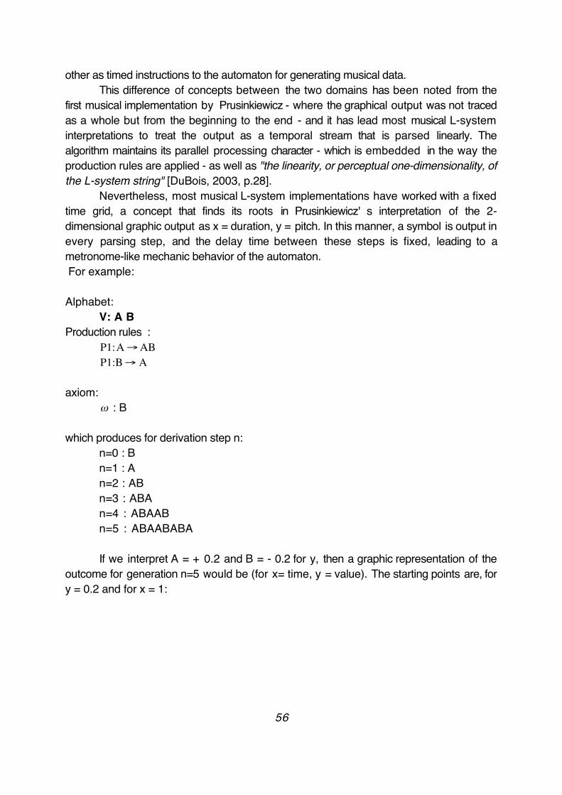
other as timed instructions to the automaton for generating musical data.This difference of concepts between the two domains has been noted from the
first musical implementation by Prusinkiewicz - where the graphical output was not traced as a whole but from the beginning to the end - and it has lead most musical L-system interpretations to treat the output as a temporal stream that is parsed linearly. The algorithm maintains its parallel processing character - which is embedded in the way the production rules are applied - as well as "the linearity, or perceptual one-dimensionality, of the L-system string" [DuBois, 2003, p.28].
Nevertheless, most musical L-system implementations have worked with a fixed time grid, a concept that finds its roots in Prusinkiewicz' s interpretation of the 2-dimensional graphic output as x = duration, y = pitch. In this manner, a symbol is output in every parsing step, and the delay time between these steps is fixed, leading to a metronome-like mechanic behavior of the automaton. For example:
Alphabet: V: A B
Production rules :
€
P1:A→AB
€
P1:B→ A axiom:
€
ω : B
which produces for derivation step n:n=0 : Bn=1 : An=2 : ABn=3 : ABAn=4 : ABAABn=5 : ABAABABA
If we interpret A = + 0.2 and B = - 0.2 for y, then a graphic representation of the outcome for generation n=5 would be (for x= time, y = value). The starting points are, for y = 0.2 and for x = 1:
56
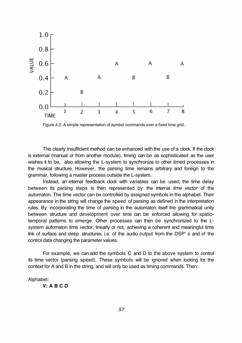
Figure 4.2: A simple representation of symbol commands over a fixed time grid.
This clearly insufficient method can be enhanced with the use of a clock. If the clock is external (manual or from another module), timing can be as sophisticated as the user wishes it to be, also allowing the L-system to synchronize to other timed processes in the musical structure. However, the parsing time remains arbitrary and foreign to the grammar, following a master process outside the L-system.
Instead, an internal feedback clock with variables can be used; the time delay between its parsing steps is then represented by the internal time vector of the automaton. The time vector can be controlled by assigned symbols in the alphabet. Their appearance in the string will change the speed of parsing as defined in the interpretation rules. By incorporating the time of parsing in the automaton itself the grammatical unity between structure and development over time can be enforced allowing for spatio-temporal patterns to emerge. Other processes can then be synchronized to the L-system automaton time vector, linearly or not, achieving a coherent and meaningful time link of surface and deep structures, i.e. of the audio output from the DSP' s and of the control data changing the parameter values.
For example, we can add the symbols C and D to the above system to control its time vector (parsing speed). These symbols will be ignored when looking for the context for A and B in the string, and will only be used as timing commands. Then:
Alphabet: V: A B C D
57
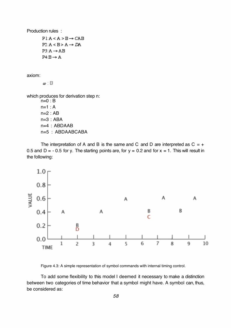
Production rules :
axiom:
which produces for derivation step n:n=0 : Bn=1 : An=2 : ABn=3 : ABAn=4 : ABDAABn=5 : ABDAABCABA
The interpretation of A and B is the same and C and D are interpreted as C = + 0.5 and D = - 0.5 for y. The starting points are, for y = 0.2 and for x = 1. This will result in the following:
Figure 4.3: A simple representation of symbol commands with internal timing control.
To add some flexibility to this model I deemed it necessary to make a distinction between two categories of time behavior that a symbol might have. A symbol can, thus, be considered as:
58
- an active time cell; the parser is going to stop after parsing such a symbol for a given time duration equal to the current state of the time vector of the branch where the symbol was encountered in.- empty time cell; the parser immediately proceeds to the next symbol in the string after parsing, with an (ideal) time lag of 0 milliseconds.
When designing a new grammar, the user needs to define which symbols in the vocabulary will be treated as active time cells.
In the above example, A and B are considered active, whereas C and D are empty time cells.
When the L-system is bracketed (with branches) the time vector can be global for all the data streams, either controlled by an external clock or by the main branch (trunk) - in which case the time vector of the trunk is used as the time vector for all the branches of the system. Otherwise, each branched automaton / data stream can use its internal, self-controlled (by the symbols it produces) time vector, allowing the model to make another step forward towards parallel data processing.
For example, using a modified bracketed version of the system above:
Alphabet: V: A B C D
Production rules :
€
P1:A < A > B→C[AB]
€
P2:A < B > A→ D[A]
€
P3:A→AB
€
P4:B→ A
axiom:
€
ω : B
which produces for derivation step n:n=0 : Bn=1 : An=2 : ABn=3 : ABAn=4 : ABD[A]ABn=5 : ABD[A][AB]ABC[AB]A
If the timing is controlled by the time vector of the main branch (trunk):
59
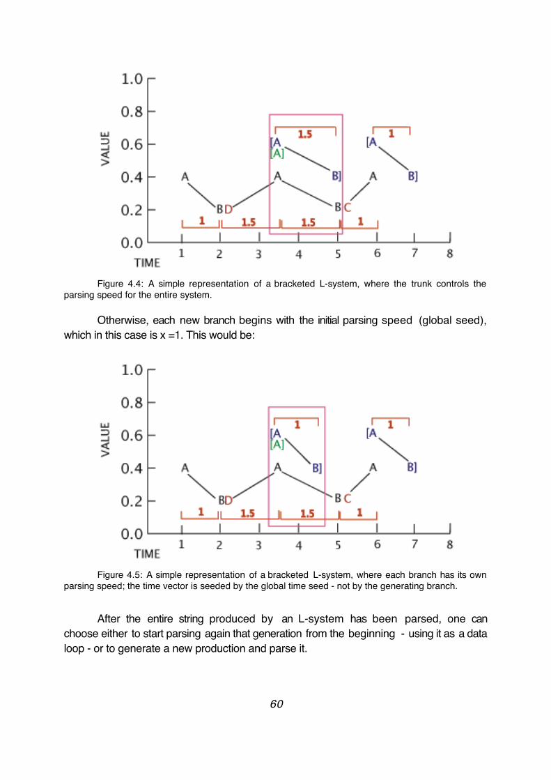
Figure 4.4: A simple representation of a bracketed L-system, where the trunk controls the parsing speed for the entire system.
Otherwise, each new branch begins with the initial parsing speed (global seed), which in this case is x =1. This would be:
Figure 4.5: A simple representation of a bracketed L-system, where each branch has its own parsing speed; the time vector is seeded by the global time seed - not by the generating branch.
After the entire string produced by an L-system has been parsed, one can choose either to start parsing again that generation from the beginning - using it as a data loop - or to generate a new production and parse it.
60
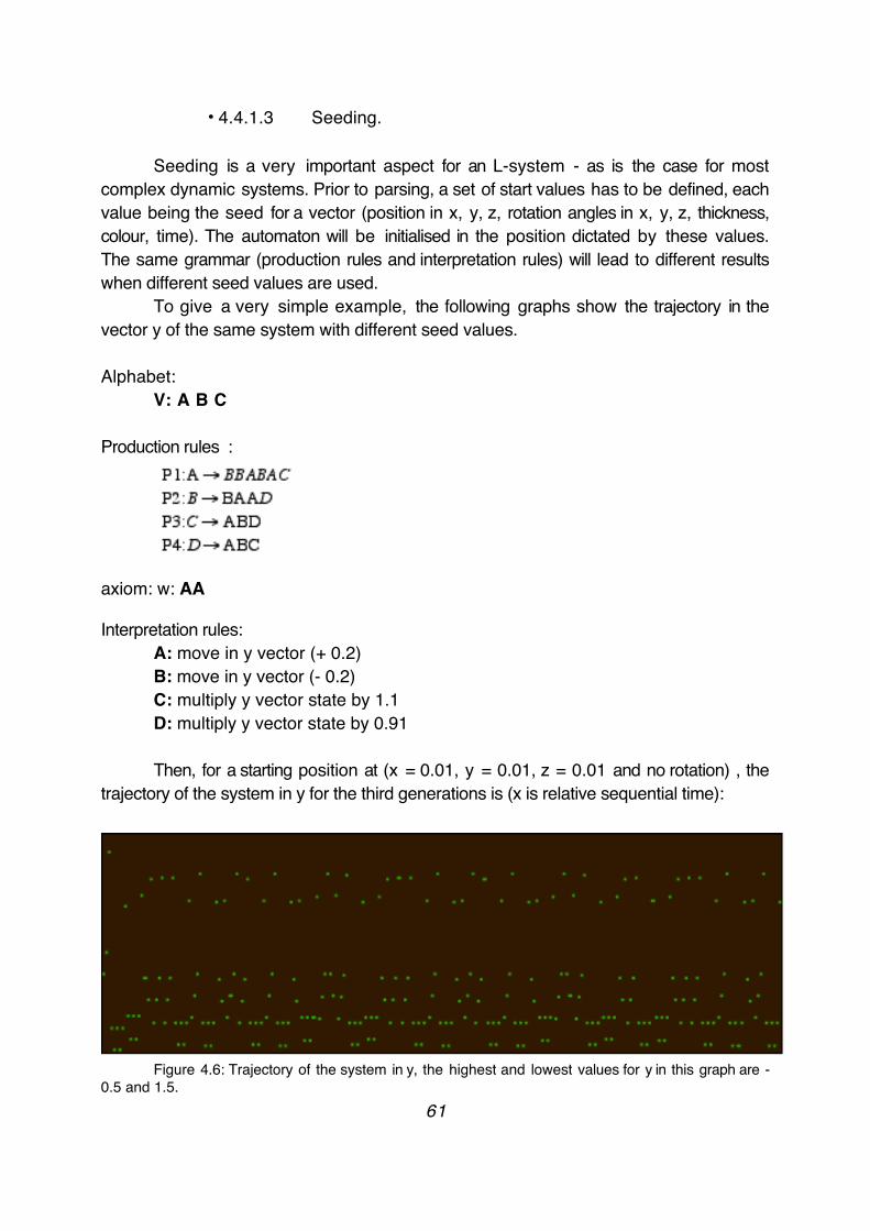
• 4.4.1.3 Seeding.
Seeding is a very important aspect for an L-system - as is the case for most complex dynamic systems. Prior to parsing, a set of start values has to be defined, each value being the seed for a vector (position in x, y, z, rotation angles in x, y, z, thickness, colour, time). The automaton will be initialised in the position dictated by these values. The same grammar (production rules and interpretation rules) will lead to different results when different seed values are used.
To give a very simple example, the following graphs show the trajectory in the vector y of the same system with different seed values.
Alphabet: V: A B C
Production rules :
axiom: w: AA
Interpretation rules:A: move in y vector (+ 0.2)B: move in y vector (- 0.2)C: multiply y vector state by 1.1D: multiply y vector state by 0.91
Then, for a starting position at (x = 0.01, y = 0.01, z = 0.01 and no rotation) , the trajectory of the system in y for the third generations is (x is relative sequential time):
Figure 4.6: Trajectory of the system in y, the highest and lowest values for y in this graph are -0.5 and 1.5.
61
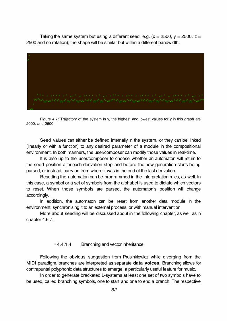
Taking the same system but using a different seed, e.g. (x = 2500, y = 2500, z = 2500 and no rotation), the shape will be similar but within a different bandwidth:
Figure 4.7: Trajectory of the system in y, the highest and lowest values for y in this graph are 2000. and 2600.
Seed values can either be defined internally in the system, or they can be linked (linearly or with a function) to any desired parameter of a module in the compositional environment. In both manners, the user/composer can modify those values in real-time.
It is also up to the user/composer to choose whether an automaton will return to the seed position after each derivation step and before the new generation starts being parsed, or instead, carry on from where it was in the end of the last derivation.
Resetting the automaton can be programmed in the interpretation rules, as well. In this case, a symbol or a set of symbols from the alphabet is used to dictate which vectors to reset. When those symbols are parsed, the automaton’s position will change accordingly.
In addition, the automaton can be reset from another data module in the environment, synchronising it to an external process, or with manual intervention.
More about seeding will be discussed about in the following chapter, as well as in chapter 4.6.7.
• 4.4.1.4 Branching and vector inheritance
Following the obvious suggestion from Prusinkiewicz while diverging from the MIDI paradigm, branches are interpreted as separate data voices. Branching allows for contrapuntal polyphonic data structures to emerge, a particularly useful feature for music.
In order to generate bracketed L-systems at least one set of two symbols have to be used, called branching symbols, one to start and one to end a branch. The respective
62

action is:
stack: use as a branching symbol:push: get the state of the generating branch and start a sub-branch.pop: end a branch and return to the state of its generating branch.
Stack options and vector inheritance:
A branch can inherit some characteristics (vector states) from its generating branch. This means that the new data stream will be seeded by the values inherited in the respective vectors. Inheritance is a property transmitted by the branching symbol that starts the new stream. It is defined in the interpretation of the branching symbol.
The stack options are in the format:
- [push/pop] vector [*]
where [*] can be any vector or combination of vectors (x, y, z, roll, yaw, pitch, thickness, colour, time). A vector can be strictly defined or selected randomly every time the branching symbol is parsed. For example, the state of a branch inheriting only the time vector from its parent branch would be the global starting point (seed) of the L-system for all vectors, except for the speed of parsing, where the seed value will be the current state of the parent branch. The two data streams will, thus, be initially in sync.
Inheritance is a particularly musical characteristic - it would not make sense in the visual world to start drawing a new branch on-the-tree in x and on-the-ground in y ; it makes sense, however, in a musical space where each vector can represent a control or synthesis parameter.
Giving an abstract musical example, in the case where the main axis (the trunk) is interpreted as an automaton controlling the global parameters of a granular synthesis engine and the starting branch as an automaton controlling one single granulator from that engine, then a stack option that pushes all the vector states of the trunk would result in:
a) setting all the parameters of that granulator to be equal to the global parameters for the engine,b) turning on the granulator,c) modulating its parameters, according to the interpretation of the symbols output by the new data stream.
Such an audio example will be given in chapter 5.
Different sets of branching symbols can be used in one grammar, allowing for the use of various types of stack operations. This permits the creation of a multitude of different possible types of dependencies and attractions between branches (the amount
63
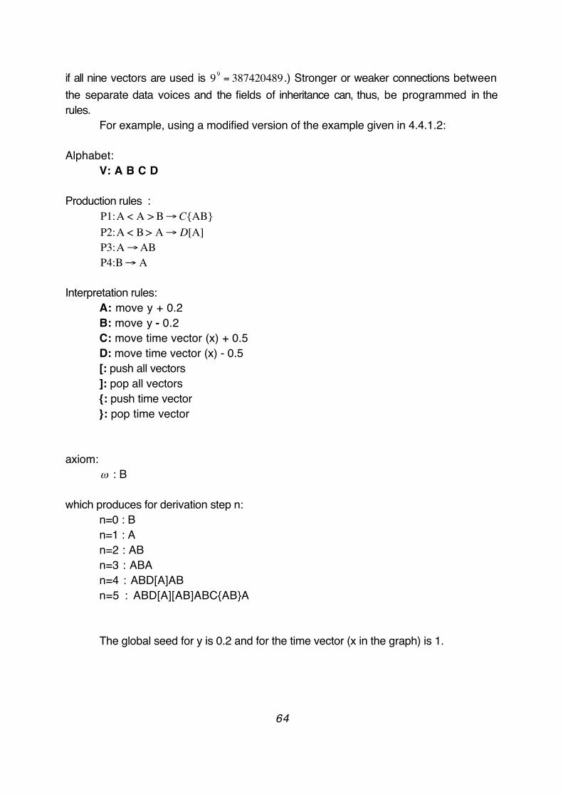
if all nine vectors are used is
€
99 = 387420489.) Stronger or weaker connections between the separate data voices and the fields of inheritance can, thus, be programmed in the rules.
For example, using a modified version of the example given in 4.4.1.2:
Alphabet: V: A B C D
Production rules :
€
P1:A < A > B→C{AB}
€
P2:A < B > A→ D[A]
€
P3:A→AB
€
P4:B→ A
Interpretation rules:A: move y + 0.2B: move y - 0.2C: move time vector (x) + 0.5D: move time vector (x) - 0.5[: push all vectors]: pop all vectors{: push time vector}: pop time vector
axiom:
€
ω : B
which produces for derivation step n:n=0 : Bn=1 : An=2 : ABn=3 : ABAn=4 : ABD[A]ABn=5 : ABD[A][AB]ABC{AB}A
The global seed for y is 0.2 and for the time vector (x in the graph) is 1.
64
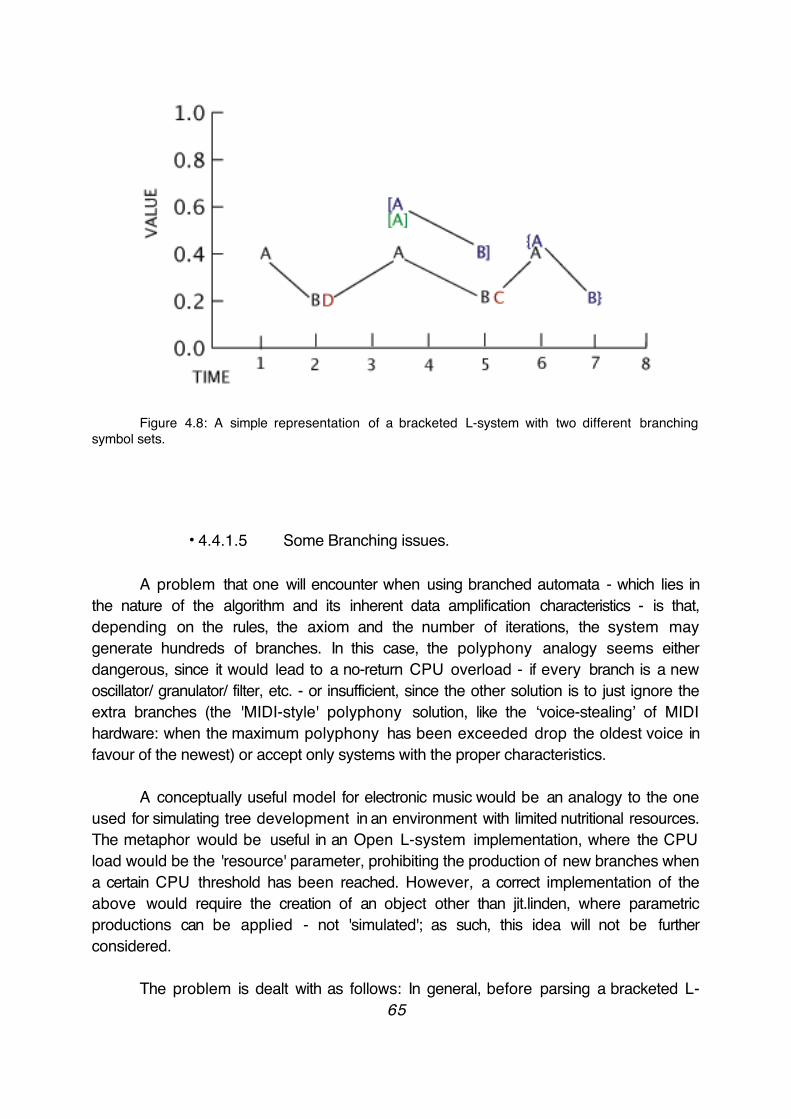
Figure 4.8: A simple representation of a bracketed L-system with two different branching symbol sets.
• 4.4.1.5 Some Branching issues.
A problem that one will encounter when using branched automata - which lies in the nature of the algorithm and its inherent data amplification characteristics - is that, depending on the rules, the axiom and the number of iterations, the system may generate hundreds of branches. In this case, the polyphony analogy seems either dangerous, since it would lead to a no-return CPU overload - if every branch is a new oscillator/ granulator/ filter, etc. - or insufficient, since the other solution is to just ignore the extra branches (the 'MIDI-style' polyphony solution, like the ‘voice-stealing’ of MIDI hardware: when the maximum polyphony has been exceeded drop the oldest voice in favour of the newest) or accept only systems with the proper characteristics.
A conceptually useful model for electronic music would be an analogy to the one used for simulating tree development in an environment with limited nutritional resources. The metaphor would be useful in an Open L-system implementation, where the CPU load would be the 'resource' parameter, prohibiting the production of new branches when a certain CPU threshold has been reached. However, a correct implementation of the above would require the creation of an object other than jit.linden, where parametric productions can be applied - not 'simulated'; as such, this idea will not be further considered.
The problem is dealt with as follows: In general, before parsing a bracketed L-65
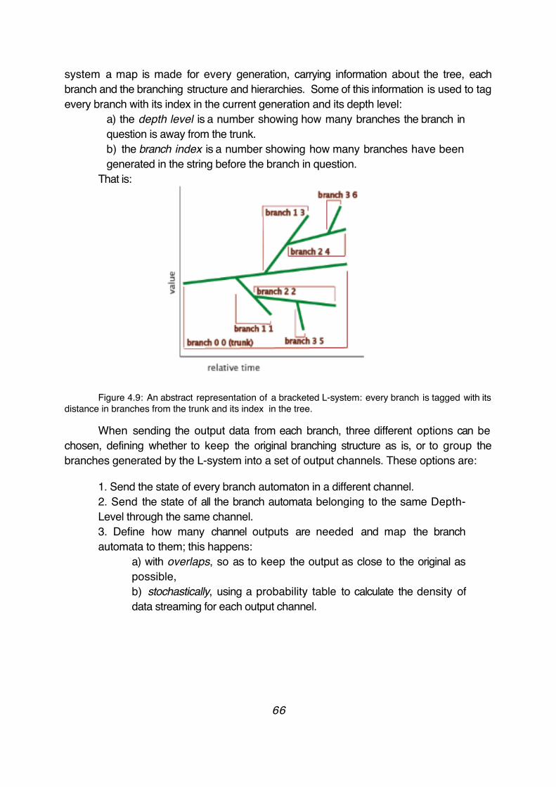
system a map is made for every generation, carrying information about the tree, each branch and the branching structure and hierarchies. Some of this information is used to tag every branch with its index in the current generation and its depth level:
a) the depth level is a number showing how many branches the branch in question is away from the trunk. b) the branch index is a number showing how many branches have been generated in the string before the branch in question.
That is:
Figure 4.9: An abstract representation of a bracketed L-system: every branch is tagged with its distance in branches from the trunk and its index in the tree.
When sending the output data from each branch, three different options can be chosen, defining whether to keep the original branching structure as is, or to group the branches generated by the L-system into a set of output channels. These options are:
1. Send the state of every branch automaton in a different channel.2. Send the state of all the branch automata belonging to the same Depth-Level through the same channel.3. Define how many channel outputs are needed and map the branch automata to them; this happens:
a) with overlaps, so as to keep the output as close to the original as possible, b) stochastically, using a probability table to calculate the density of data streaming for each output channel.
66

For example, using again a modified version of the L-system from chapter 4.4.1.2:
Alphabet: V: A B C D
Production rules :
€
P1:* < A > B→ A{CAB}D
€
P2:* < B > A→ [DA]C
€
P3:A→AB
€
P4:B→ A
Interpretation rules:A: move y + 0.2B: move y - 0.2C: move time vector (x) + 0.5D: move time vector (x) - 0.5[: push all vectors]: pop all vectors{: push time vector}: pop time vector
axiom:
€
ω : B
which produces for derivation step n:n=0 : Bn=1 : An=2 : ABn=3 : A{CAB}DAn=4 : AB{A{CAB}DA}ABn=5 : A{AB{A{CAB}DA}AB}A{CAB}D[DA]C
67

Figure 4.10: A simple representation of a bracketed L-system with branches grouped by depth level . When there are two simultaneous values from different branches they will be output one after the other with a time delay of 0 milliseconds.
The third option is, by far, the most useful and versatile. When overlapping is used, minor data distortion occurs - depending, of course, on the ratio of real branches to output branches. The distortion effect can be minimized by adding a Table L-system
68
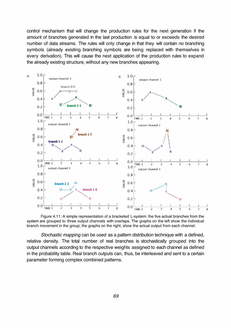
control mechanism that will change the production rules for the next generation if the amount of branches generated in the last production is equal to or exceeds the desired number of data streams. The rules will only change in that they will contain no branching symbols (already existing branching symbols are being replaced with themselves in every derivation). This will cause the next application of the production rules to expand the already existing structure, without any new branches appearing.
Figure 4.11: A simple representation of a bracketed L-system: the five actual branches from the system are grouped to three output channels with overlaps. The graphs on the left show the individual branch movement in the group; the graphs on the right, show the actual output from each channel.
Stochastic mapping can be used as a pattern distribution technique with a defined, relative density. The total number of real branches is stochastically grouped into the output channels according to the respective weights assigned to each channel as defined in the probability table. Real branch outputs can, thus, be interleaved and sent to a certain parameter forming complex combined patterns.
69
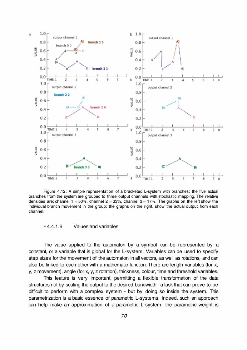
Figure 4.12: A simple representation of a bracketed L-system with branches: the five actual branches from the system are grouped to three output channels with stochastic mapping. The relative densities are: channel 1 = 50%, channel 2 = 33%, channel 3 = 17%. The graphs on the left show the individual branch movement in the group; the graphs on the right, show the actual output from each channel.
• 4.4.1.6 Values and variables
The value applied to the automaton by a symbol can be represented by a constant, or a variable that is global for the L-system. Variables can be used to specify step sizes for the movement of the automaton in all vectors, as well as rotations, and can also be linked to each other with a mathematic function. There are length variables (for x, y, z movement), angle (for x, y, z rotation), thickness, colour, time and threshold variables.
This feature is very important, permitting a flexible transformation of the data structures not by scaling the output to the desired bandwidth - a task that can prove to be difficult to perform with a complex system - but by doing so inside the system. This parametrization is a basic essence of parametric L-systems. Indeed, such an approach can help make an approximation of a parametric L-system; the parametric weight is
70
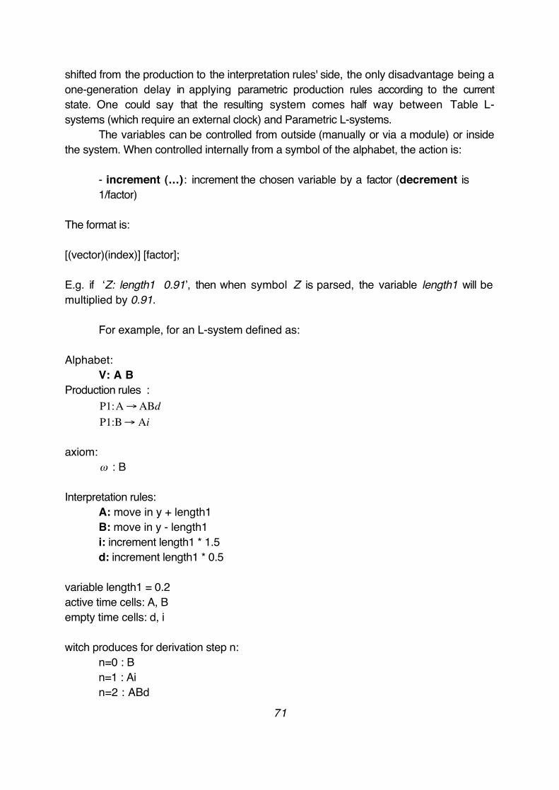
shifted from the production to the interpretation rules' side, the only disadvantage being a one-generation delay in applying parametric production rules according to the current state. One could say that the resulting system comes half way between Table L-systems (which require an external clock) and Parametric L-systems.
The variables can be controlled from outside (manually or via a module) or inside the system. When controlled internally from a symbol of the alphabet, the action is:
- increment (...): increment the chosen variable by a factor (decrement is 1/factor)
The format is: [(vector)(index)] [factor];
E.g. if ‘Z: length1 0.91’, then when symbol Z is parsed, the variable length1 will be multiplied by 0.91.
For example, for an L-system defined as:
Alphabet: V: A B
Production rules :
€
P1:A→ABd
€
P1:B→ Ai
axiom:
€
ω : B
Interpretation rules:A: move in y + length1B: move in y - length1i: increment length1 * 1.5d: increment length1 * 0.5
variable length1 = 0.2active time cells: A, Bempty time cells: d, i
witch produces for derivation step n:n=0 : Bn=1 : Ain=2 : ABd
71
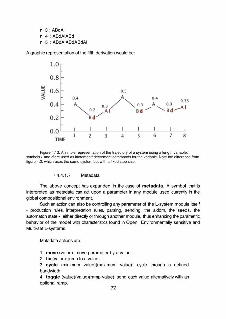
n=3 : ABdAin=4 : ABdAiABdn=5 : ABdAiABdABdAi
A graphic representation of the fifth derivation would be:
Figure 4.13: A simple representation of the trajectory of a system using a length variable; symbols i and d are used as increment/ decrement commands for the variable. Note the difference from figure 4.2, which uses the same system but with a fixed step size.
• 4.4.1.7 Metadata
The above concept has expanded in the case of metadata. A symbol that is interpreted as metadata can act upon a parameter in any module used currently in the global compositional environment.
Such an action can also be controlling any parameter of the L-system module itself - production rules, interpretation rules, parsing, sending, the axiom, the seeds, the automaton state - either directly or through another module, thus enhancing the parametric behavior of the model with characteristics found in Open, Environmentally sensitive and Multi-set L-systems.
Metadata actions are:
1. move (value): move parameter by a value.2. fix (value): jump to a value.3. cycle (minimum value)(maximum value): cycle through a defined bandwidth.4. toggle (value)(value)(ramp-value): send each value alternatively with an optional ramp.
72
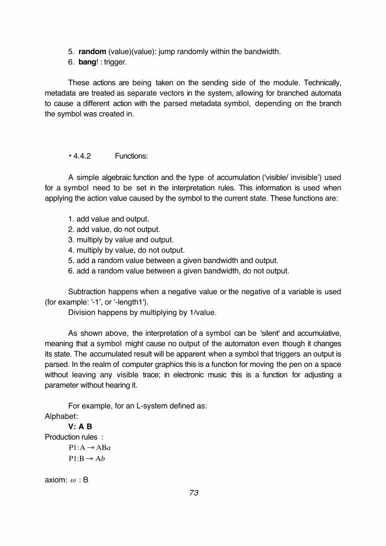
5. random (value)(value): jump randomly within the bandwidth.6. bang! : trigger.
These actions are being taken on the sending side of the module. Technically, metadata are treated as separate vectors in the system, allowing for branched automata to cause a different action with the parsed metadata symbol, depending on the branch the symbol was created in.
• 4.4.2 Functions:
A simple algebraic function and the type of accumulation (‘visible/ invisible’) used for a symbol need to be set in the interpretation rules. This information is used when applying the action value caused by the symbol to the current state. These functions are:
1. add value and output.2. add value, do not output.3. multiply by value and output.4. multiply by value, do not output.5. add a random value between a given bandwidth and output.6. add a random value between a given bandwidth, do not output.
Subtraction happens when a negative value or the negative of a variable is used (for example: '-1’, or ‘-length1').
Division happens by multiplying by 1/value.
As shown above, the interpretation of a symbol can be 'silent' and accumulative, meaning that a symbol might cause no output of the automaton even though it changes its state. The accumulated result will be apparent when a symbol that triggers an output is parsed. In the realm of computer graphics this is a function for moving the pen on a space without leaving any visible trace; in electronic music this is a function for adjusting a parameter without hearing it.
For example, for an L-system defined as:Alphabet:
V: A BProduction rules :
€
P1:A→ABa
€
P1:B→ Ab
axiom:
€
ω : B73
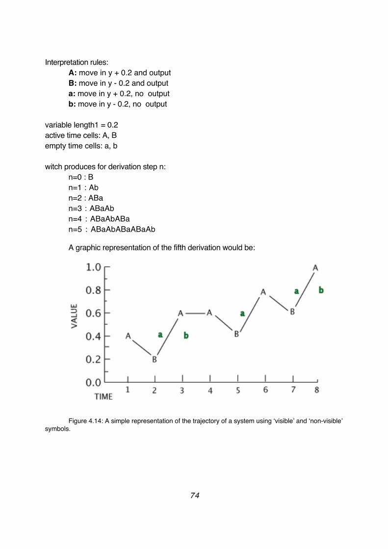
Interpretation rules:A: move in y + 0.2 and outputB: move in y - 0.2 and outputa: move in y + 0.2, no outputb: move in y - 0.2, no output
variable length1 = 0.2active time cells: A, Bempty time cells: a, b
witch produces for derivation step n:n=0 : Bn=1 : Abn=2 : ABan=3 : ABaAbn=4 : ABaAbABan=5 : ABaAbABaABaAb
A graphic representation of the fifth derivation would be:
Figure 4.14: A simple representation of the trajectory of a system using ‘visible’ and ‘non-visible’ symbols.
74
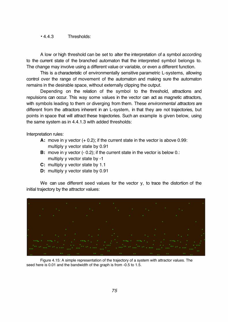
• 4.4.3 Thresholds:
A low or high threshold can be set to alter the interpretation of a symbol according to the current state of the branched automaton that the interpreted symbol belongs to. The change may involve using a different value or variable, or even a different function.
This is a characteristic of environmentally sensitive parametric L-systems, allowing control over the range of movement of the automaton and making sure the automaton remains in the desirable space, without externally clipping the output.
Depending on the relation of the symbol to the threshold, attractions and repulsions can occur. This way some values in the vector can act as magnetic attractors, with symbols leading to them or diverging from them. These environmental attractors are different from the attractors inherent in an L-system, in that they are not trajectories, but points in space that will attract these trajectories. Such an example is given below, using the same system as in 4.4.1.3 with added thresholds:
Interpretation rules:A: move in y vector (+ 0.2); if the current state in the vector is above 0.99: multiply y vector state by 0.91B: move in y vector (- 0.2); if the current state in the vector is below 0.: multiply y vector state by -1C: multiply y vector state by 1.1D: multiply y vector state by 0.91
We can use different seed values for the vector y, to trace the distortion of the initial trajectory by the attractor values:
Figure 4.15: A simple representation of the trajectory of a system with attractor values. The seed here is 0.01 and the bandwidth of the graph is from -0.5 to 1.5.
75
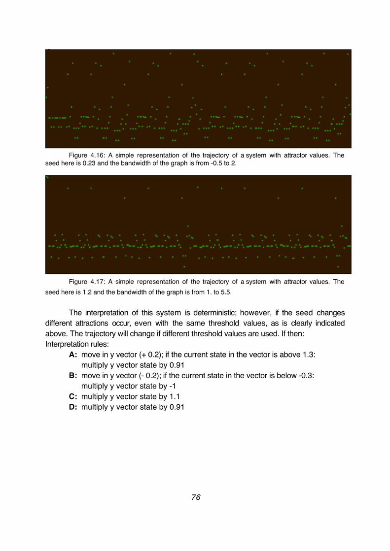
Figure 4.16: A simple representation of the trajectory of a system with attractor values. The seed here is 0.23 and the bandwidth of the graph is from -0.5 to 2.
Figure 4.17: A simple representation of the trajectory of a system with attractor values. The seed here is 1.2 and the bandwidth of the graph is from 1. to 5.5.
The interpretation of this system is deterministic; however, if the seed changes different attractions occur, even with the same threshold values, as is clearly indicated above. The trajectory will change if different threshold values are used. If then:Interpretation rules:
A: move in y vector (+ 0.2); if the current state in the vector is above 1.3: multiply y vector state by 0.91B: move in y vector (- 0.2); if the current state in the vector is below -0.3: multiply y vector state by -1C: multiply y vector state by 1.1D: multiply y vector state by 0.91
76
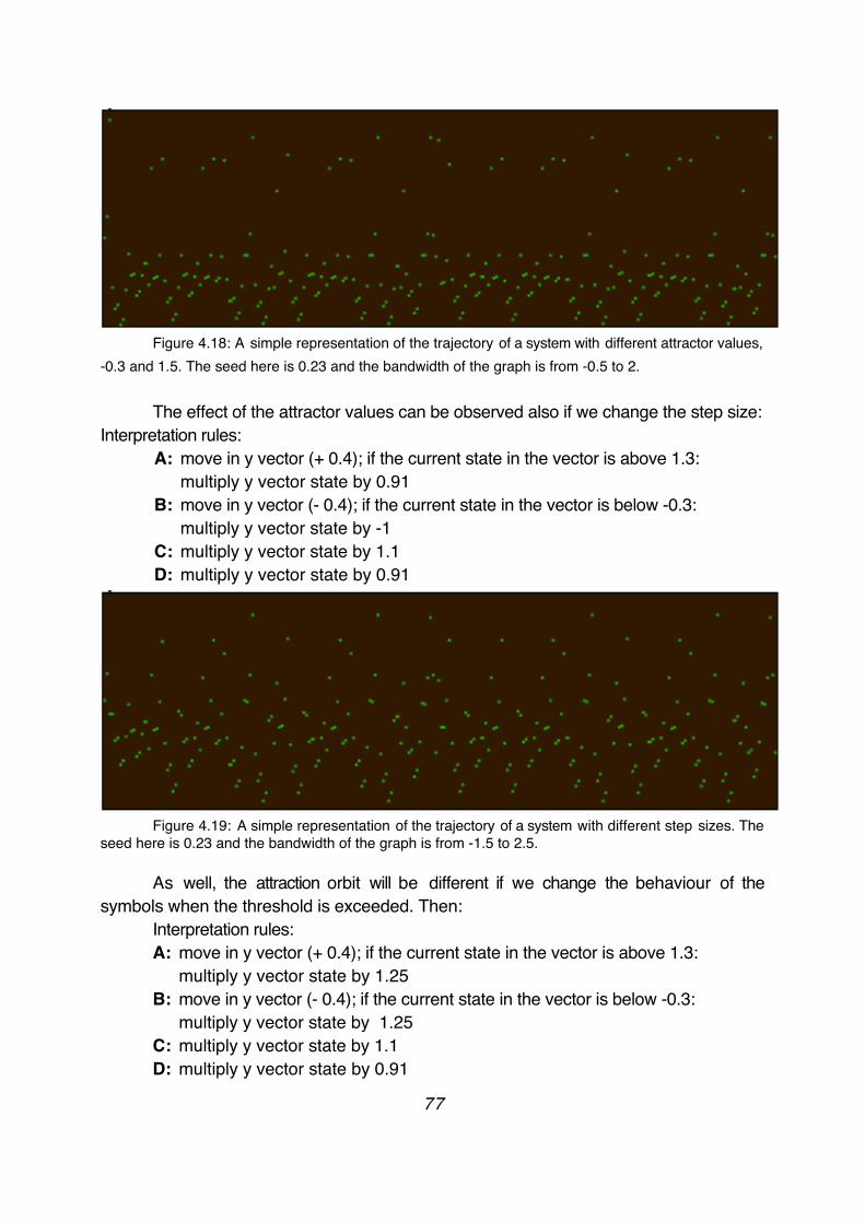
Figure 4.18: A simple representation of the trajectory of a system with different attractor values, -0.3 and 1.5. The seed here is 0.23 and the bandwidth of the graph is from -0.5 to 2.
The effect of the attractor values can be observed also if we change the step size:Interpretation rules:
A: move in y vector (+ 0.4); if the current state in the vector is above 1.3: multiply y vector state by 0.91B: move in y vector (- 0.4); if the current state in the vector is below -0.3: multiply y vector state by -1C: multiply y vector state by 1.1D: multiply y vector state by 0.91
Figure 4.19: A simple representation of the trajectory of a system with different step sizes. The seed here is 0.23 and the bandwidth of the graph is from -1.5 to 2.5.
As well, the attraction orbit will be different if we change the behaviour of the symbols when the threshold is exceeded. Then:
Interpretation rules:A: move in y vector (+ 0.4); if the current state in the vector is above 1.3: multiply y vector state by 1.25B: move in y vector (- 0.4); if the current state in the vector is below -0.3: multiply y vector state by 1.25C: multiply y vector state by 1.1D: multiply y vector state by 0.91
77
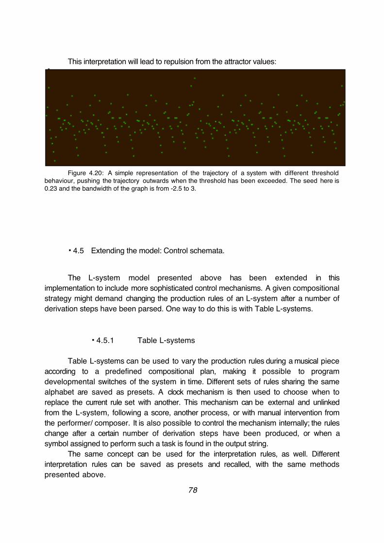
This interpretation will lead to repulsion from the attractor values:
Figure 4.20: A simple representation of the trajectory of a system with different threshold behaviour, pushing the trajectory outwards when the threshold has been exceeded. The seed here is 0.23 and the bandwidth of the graph is from -2.5 to 3.
• 4.5 Extending the model: Control schemata.
The L-system model presented above has been extended in this implementation to include more sophisticated control mechanisms. A given compositional strategy might demand changing the production rules of an L-system after a number of derivation steps have been parsed. One way to do this is with Table L-systems.
• 4.5.1 Table L-systems
Table L-systems can be used to vary the production rules during a musical piece according to a predefined compositional plan, making it possible to program developmental switches of the system in time. Different sets of rules sharing the same alphabet are saved as presets. A clock mechanism is then used to choose when to replace the current rule set with another. This mechanism can be external and unlinked from the L-system, following a score, another process, or with manual intervention from the performer/ composer. It is also possible to control the mechanism internally; the rules change after a certain number of derivation steps have been produced, or when a symbol assigned to perform such a task is found in the output string.
The same concept can be used for the interpretation rules, as well. Different interpretation rules can be saved as presets and recalled, with the same methods presented above.
78
• 4.5.2 Evolving grammars
A non-deterministic extension of TL-systems is implemented using genetic algorithms (GA). A genetic algorithm is a particular class of Evolutionary computation, which in itself is a subfield of Artificial Intelligence. GAs are used in computer science as a technique for finding approximate solutions to search and optimization problems.
The algorithm is a simulation of natural evolution inspired by evolutionary biology. The same terminology is used. The genotype is the genetic information that contains the codes for the creation of the individual; that is the DNA of the organism in organic life or a string consisting of bits, integers, or symbols in the case of simulations. The individual - object or system - created from the genotype is known as the phenotype. Genetic variation is achieved through reproduction, which is simulated with crossover and mutation. Crossover combines different genotypes into one, while mutation randomly alters portions of the genome. The fitness of an organism, determined by its ability to survive and pass on its genes from generation to generation, is determined by selection. In a real world environment fitness is a very complex procedure. In simulated genetic systems, the fitness can be determined automatically, by a defined fitness function, or interactively, by the choices of a human user.
The origins of Evolutionary computation are found in John Holland's studies of cellular automata. In 'Adaptation in Natural and Artificial Systems', he described how the evolutionary process in nature can be applied to artificial systems using the Darwinian operation of fitness proportionate reproduction and the genetic operation of recombination operating on fixed length character strings. The algorithm remained a theoretical framework until advancements in CPU power allowed for practical applications.
Richard Dawkins [Dawkins, 1987] proposes that evolution happens through accumulations of small changes in the genetic code that assure the survival of the fittest in an environment. He models the evolution of organisms called 'biomorphs', which are graphic images drawn recursively by a subdivision algorithm. The genetic code is the vector driving this algorithm.
Evolutionary models profit from using an abstract generative method encoding data structures. A generative representation of the possible structures instead of a non-generative one is much more powerful, as shown in [Hornby-Pollack, 2001b]. Generative representations are defined in [Hornby-Pollack, 2003b] as "a class of representations in which elements in the encoded data structure of a design can be reused in creating the design."
One of the most promising methods of genome encoding is with L-systems. The gene is not represented by a bit-string, as the case is usually, but by symbols. Lately there has been some very interesting research combining Evolutionary computation and
79
L-systems with some impressive results, see [Ochoa, 1998], [Hornby-Pollack: 2001a, 2001b, 2002, 2003a, 2003b]. The general goal is to solve the 'inference' or inverse problem, or else, to create the rules for producing a desired type of structure .
The advantages of using genetic algorithms to evolve the rules of a musical L-system are:
1. Rule spaces can be investigated as Genome spaces prior to composing. A known problem when using L-systems is writing the proper production rules that would generate a desired output, a difficult process common to fractal algorithms that is referred to as the 'inference' problem [Koza, 1993]. Whereas it is a relatively easy task to compose the alphabet set and the interpretation rules, the compactness and abstractness of the production rules can make the relations between them and the actual output obscure, especially for large and complicated systems. Genetic algorithms facilitate this procedure by recursively performing crossovers and mutations over a seed set of production rules and choosing the next parent according to a fitness function.2. Stochastic variations of the rules can be generated with mutation and crossover, thus changing the structure of the output towards a goal defined in the fitness function.
The model works as follows:
- Initialization:
The composer first has to define the alphabet, assign the interpretation and decomposition rules to each symbol in the alphabet, and provide a seed rule-set. The successor side of the rule-set can be random, though it is usually more effective to give some structural guideline about branching structures. The predecessors, however, need to be explicitly defined in order to make productions of a certain type (context-free, context-dependent).
- Providing the fitness function:
The module performing the evolutionary computation contains a set of parameters. These include:
1. The amount of offspring to produce.2. The genetic operations to be used (mutation/ crossover). 3. The probability percentage of mutation and crossover. 4. Setting the range of mutation for a specific segment element to the n closest genes.
80
5. The type of fitness function to be used.6. How fit the next parent should be.
The fitness function is used here more as a way to manipulate variation than as a method for obtaining a concretely defined result. The goal is not to imitate a given structure but to recursively generate new and unknown ones by controlling the direction of evolution. Fitness can be decided automatically or interactively. When interactive, the composer manually selects which offspring to reproduce. When automated, there are three fitness function categories:
-Test mode. The offspring are compared to the parent according to a set comparison operator (=, >=, <=, >, <). They are then categorized according to how close or far to the ideal result they are. (e.g. when using '=' equal is best, etc.) - Mutation. The offspring are categorized according to the amount of mutation when compared to the parent.- Statistics. The offspring are put in order (from minimum to maximum) according to a statistic analysis (bandwidth, mean, average deviation, standard deviation, variance, skew, kurtosis.)
Fitness is measured relatively by comparing all offspring and putting them in order according to the function. The fitness index is then used to choose how fit an offspring should be to use it as the next parent.
- Mutation:
Mutation is the main technique used for evolving grammars. Researchers have applied mutations to both symbols and parameters in a production; however, due to the limitations of jit.linden and its inability to generate parametric productions, only symbol mutation can occur. Variables can also be mutated, but this has a different effect when happening on the interpretation side of the algorithm. Possible mutations are:
1. A symbol in a production may be removed.2. A symbol in a production may be added.3. A symbol in a production may change to another symbol.
This can have as a consequence:4. A rule is created if a symbol does not have one. If a symbol in the alphabet is not included as a predecessor in the rule set, it is considered to have an empty successor. Through mutation a non-empty word can take this place, adding a rule in the system.
81
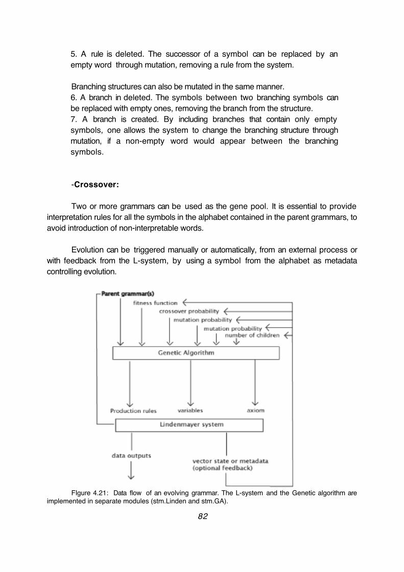
5. A rule is deleted. The successor of a symbol can be replaced by an empty word through mutation, removing a rule from the system.
Branching structures can also be mutated in the same manner. 6. A branch in deleted. The symbols between two branching symbols can be replaced with empty ones, removing the branch from the structure.7. A branch is created. By including branches that contain only empty symbols, one allows the system to change the branching structure through mutation, if a non-empty word would appear between the branching symbols.
-Crossover:
Two or more grammars can be used as the gene pool. It is essential to provide interpretation rules for all the symbols in the alphabet contained in the parent grammars, to avoid introduction of non-interpretable words.
Evolution can be triggered manually or automatically, from an external process or with feedback from the L-system, by using a symbol from the alphabet as metadata controlling evolution.
FIgure 4.21: Data flow of an evolving grammar. The L-system and the Genetic algorithm are implemented in separate modules (stm.Linden and stm.GA).
82
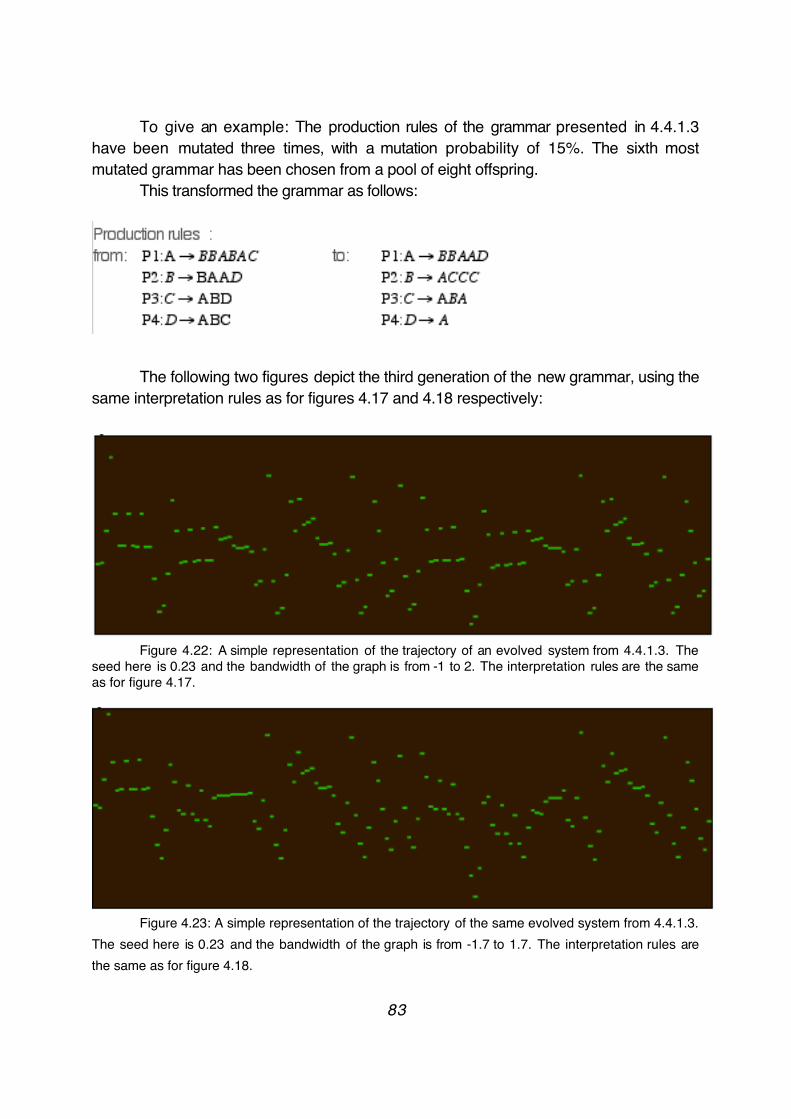
To give an example: The production rules of the grammar presented in 4.4.1.3 have been mutated three times, with a mutation probability of 15%. The sixth most mutated grammar has been chosen from a pool of eight offspring.
This transformed the grammar as follows:
The following two figures depict the third generation of the new grammar, using the same interpretation rules as for figures 4.17 and 4.18 respectively:
Figure 4.22: A simple representation of the trajectory of an evolved system from 4.4.1.3. The seed here is 0.23 and the bandwidth of the graph is from -1 to 2. The interpretation rules are the same as for figure 4.17.
Figure 4.23: A simple representation of the trajectory of the same evolved system from 4.4.1.3. The seed here is 0.23 and the bandwidth of the graph is from -1.7 to 1.7. The interpretation rules are the same as for figure 4.18.
83
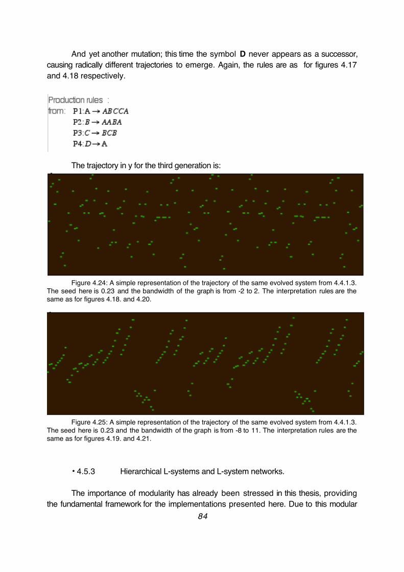
And yet another mutation; this time the symbol D never appears as a successor, causing radically different trajectories to emerge. Again, the rules are as for figures 4.17 and 4.18 respectively.
The trajectory in y for the third generation is:
Figure 4.24: A simple representation of the trajectory of the same evolved system from 4.4.1.3. The seed here is 0.23 and the bandwidth of the graph is from -2 to 2. The interpretation rules are the same as for figures 4.18. and 4.20.
Figure 4.25: A simple representation of the trajectory of the same evolved system from 4.4.1.3. The seed here is 0.23 and the bandwidth of the graph is from -8 to 11. The interpretation rules are the same as for figures 4.19. and 4.21.
• 4.5.3 Hierarchical L-systems and L-system networks.
The importance of modularity has already been stressed in this thesis, providing the fundamental framework for the implementations presented here. Due to this modular
84
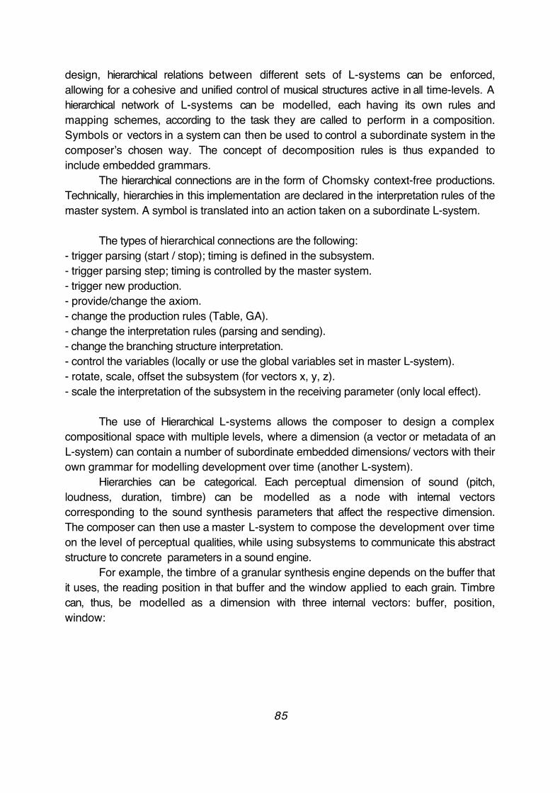
design, hierarchical relations between different sets of L-systems can be enforced, allowing for a cohesive and unified control of musical structures active in all time-levels. A hierarchical network of L-systems can be modelled, each having its own rules and mapping schemes, according to the task they are called to perform in a composition. Symbols or vectors in a system can then be used to control a subordinate system in the composer’s chosen way. The concept of decomposition rules is thus expanded to include embedded grammars.
The hierarchical connections are in the form of Chomsky context-free productions. Technically, hierarchies in this implementation are declared in the interpretation rules of the master system. A symbol is translated into an action taken on a subordinate L-system.
The types of hierarchical connections are the following:- trigger parsing (start / stop); timing is defined in the subsystem.- trigger parsing step; timing is controlled by the master system.- trigger new production.- provide/change the axiom.- change the production rules (Table, GA).- change the interpretation rules (parsing and sending).- change the branching structure interpretation.- control the variables (locally or use the global variables set in master L-system).- rotate, scale, offset the subsystem (for vectors x, y, z).- scale the interpretation of the subsystem in the receiving parameter (only local effect).
The use of Hierarchical L-systems allows the composer to design a complex compositional space with multiple levels, where a dimension (a vector or metadata of an L-system) can contain a number of subordinate embedded dimensions/ vectors with their own grammar for modelling development over time (another L-system).
Hierarchies can be categorical. Each perceptual dimension of sound (pitch, loudness, duration, timbre) can be modelled as a node with internal vectors corresponding to the sound synthesis parameters that affect the respective dimension. The composer can then use a master L-system to compose the development over time on the level of perceptual qualities, while using subsystems to communicate this abstract structure to concrete parameters in a sound engine.
For example, the timbre of a granular synthesis engine depends on the buffer that it uses, the reading position in that buffer and the window applied to each grain. Timbre can, thus, be modelled as a dimension with three internal vectors: buffer, position, window:
85
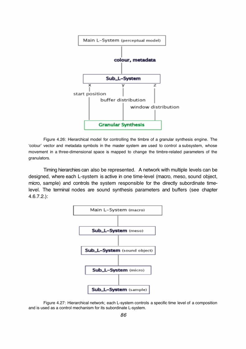
Figure 4.26: Hierarchical model for controlling the timbre of a granular synthesis engine. The ‘colour’ vector and metadata symbols in the master system are used to control a subsystem, whose movement in a three-dimensional space is mapped to change the timbre-related parameters of the granulators.
Timing hierarchies can also be represented. A network with multiple levels can be designed, where each L-system is active in one time-level (macro, meso, sound object, micro, sample) and controls the system responsible for the directly subordinate time-level. The terminal nodes are sound synthesis parameters and buffers (see chapter 4.6.7.2.):
Figure 4.27: Hierarchical network; each L-system controls a specific time level of a composition and is used as a control mechanism for its subordinate L-system.
86
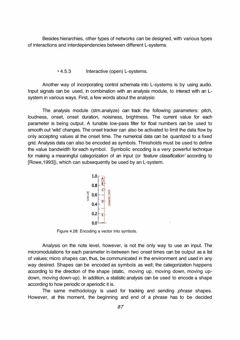
Besides hierarchies, other types of networks can be designed, with various types of interactions and interdependencies between different L-systems.
• 4.5.3 Interactive (open) L-systems.
Another way of incorporating control schemata into L-systems is by using audio. Input signals can be used, in combination with an analysis module, to interact with an L-system in various ways. First, a few words about the analysis:
The analysis module (stm.analyze) can track the following parameters: pitch, loudness, onset, onset duration, noisiness, brightness. The current value for each parameter is being output. A tunable low-pass filter for float numbers can be used to smooth out ‘wild’ changes. The onset tracker can also be activated to limit the data flow by only accepting values at the onset time. The numerical data can be quantized to a fixed grid. Analysis data can also be encoded as symbols. Thresholds must be used to define the value bandwidth for each symbol. Symbolic encoding is a very powerful technique for making a meaningful categorization of an input (or ‘feature classification’ according to [Rowe,1993]), which can subsequently be used by an L-system.
Figure 4.28: Encoding a vector into symbols.
Analysis on the note level, however, is not the only way to use an input. The micromodulations for each parameter in-between two onset times can be output as a list of values; micro shapes can, thus, be communicated in the environment and used in any way desired. Shapes can be encoded as symbols as well; the categorization happens according to the direction of the shape (static, moving up, moving down, moving up-down, moving down-up). In addition, a statistic analysis can be used to encode a shape according to how periodic or aperiodic it is.
The same methodology is used for tracking and sending phrase shapes. However, at this moment, the beginning and end of a phrase has to be decided
87
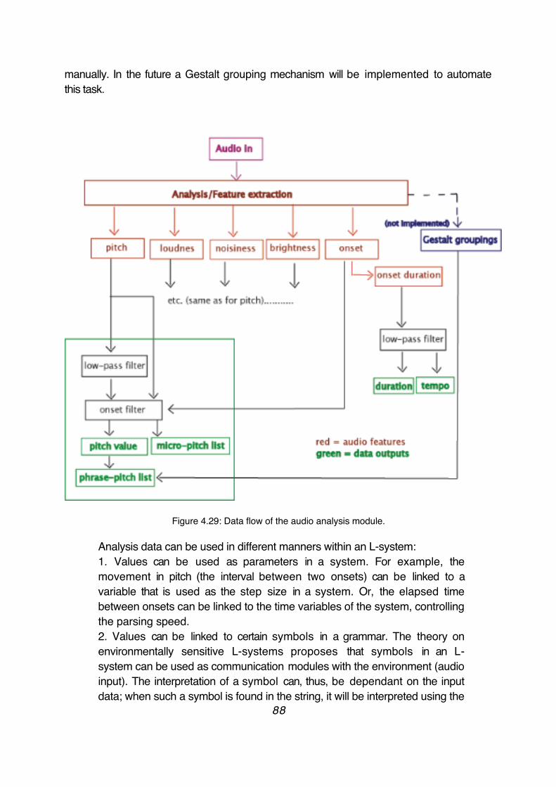
manually. In the future a Gestalt grouping mechanism will be implemented to automate this task.
Figure 4.29: Data flow of the audio analysis module.
Analysis data can be used in different manners within an L-system:1. Values can be used as parameters in a system. For example, the movement in pitch (the interval between two onsets) can be linked to a variable that is used as the step size in a system. Or, the elapsed time between onsets can be linked to the time variables of the system, controlling the parsing speed. 2. Values can be linked to certain symbols in a grammar. The theory on environmentally sensitive L-systems proposes that symbols in an L-system can be used as communication modules with the environment (audio input). The interpretation of a symbol can, thus, be dependant on the input data; when such a symbol is found in the string, it will be interpreted using the
88

current value of the input in the assigned analysis vector (e.g. pitch value).3. Values encoded as symbols can function as the axiom for an L-system. The encoded data will be amplified by the system after every iteration, parsed and sent as controls for a process in the compositional environment. 4. Shapes can be treated as objects (see chapter 4.6.5.). The symbols from the L-system will then be used to choose which object/shape to send as control to a process. 5. A shape can be used as the seed for a table interpretation (list, matrix or waveform) of an L-system. This will be explained in chapter 4.6.7.
An interactive L-system would profit from an object different than ‘jit.linden’ that would use parametric production rules. The input could be directly linked to the system as its set of numerical parameters, having an effect on the produced string.
A very promising idea for further research would be to make an L-system audio-structure analyser. The audio input would be parsed and encoded in the form of a generative grammar, with an alphabet, production rules and axiom. This grammar, modified according to the compositional plan, would be then used to re-synthesize the structure of the input in any desired manner. In order to implement this the inference problem should be solved - or how to go from the surface to the deep structure. The method should be similar to the one implemented in the SEQUITUR program - a software using L-systems to “develop simple, robust techniques that reveal interesting structure in a wide range of real-world sequences including music, English text, descriptions of plants, graphical figures, DNA sequences, word classes in language, a genealogical database, programming languages, execution traces, and diverse sequences from a data compression corpus.” [Nevill-Manning, 1996]. This is, however, out of the scope of this thesis.
• 4.6 Mapping schemes.
The decision in this implementation was to provide the platform for a flexible mapping of the data produced by the L-systems, permitting the simultaneous use of various strategies of interpretation.
89
• 4.6.1 Event-literal symbol mapping.
The most obvious way to map the output of an L-system is to treat each symbol as a discrete event generator. This is the case, for example, in McCormack' s implementation, where each symbol is translated as a note. This is the simplest and most straightforward way of mapping, though it lacks flexibility. A deterministic L-system with event-literal mapping will always have exactly the same output.
An event-literal mapping can generate interesting repeating structures, expressed as local relations between symbols, without much pre-compositional effort. Such a mapping is more powerful when used in a higher time level, as a control-schema for subordinate processes or subordinate L-systems, than when functioning as a terminal data node. The results, of course, will be much more interesting when a context-sensitive L-system is being used.
A very basic example of such a mapping is given below, using Lindenmayer' s system for algae growth (shown in chapter 2.5.3):
Alphabet: V: A B
Production rules :
€
P1:A→AB
€
P1:B→ A axiom:
€
ω : B
which produces for derivation step n:n=0 : Bn=1 : An=2 : ABn=3 : ABAn=4 : ABAABn=5 : ABAABABA n=6 : ABAABABAABAABn=7 : ABAABABAABAABABAABABAn=8 : ABAABABAABAABABAABABAABAABABAABAAB
One of the simplest ways to map this output is by assigning one symbol to be an ON value of some kind, and the other an OFF value of the same kind:
A = ON / note / trigger / 1B = OFF / rest / gate / 0
90

The output would then be:
n=0 : 0n=1 : 1n=2 : 10n=3 : 101n=4 : 10110n=5 : 10110101 n=6 : 1011010110110n=7 : 10110101101101101010
or graphically:
Figure 4.30: A simple ‘binary’ graphic representation of the first eight generations of Lindenmayer’s system for modelling algae growth.
• 4.6.2 Movement mapping (relative spatial mapping).
There has been alot of research on spatial representations of musical structures. Navigation of a parameter space is one of the most prominent issues in current electronic music thought. Gestural controllers and algorithms are widely used to navigate a space defined by the composer.
In this interpretation, every vector of the automaton can be mapped to a parameter, allowing the turtle to move in the compositional space. A symbol in the alphabet can be translated into a command that moves the turtle automaton in a vector or a combination of vectors. It is important to decouple the actual position of the turtle in each vector from the output value. The output of the system is, thus, mapped iteratively to a parameter in the environment. As such, the movement of the turtle controls the contour/ trajectory of the slave parameter, not the absolute position. Decoupling the internal state of the systems from the actual value is mandated for the following reasons:
- The output of a complex system depends on the seed value. Tracking the movement instead of position allows experimentation with different seeds, without having to worry about the absolute state of the automaton.
91
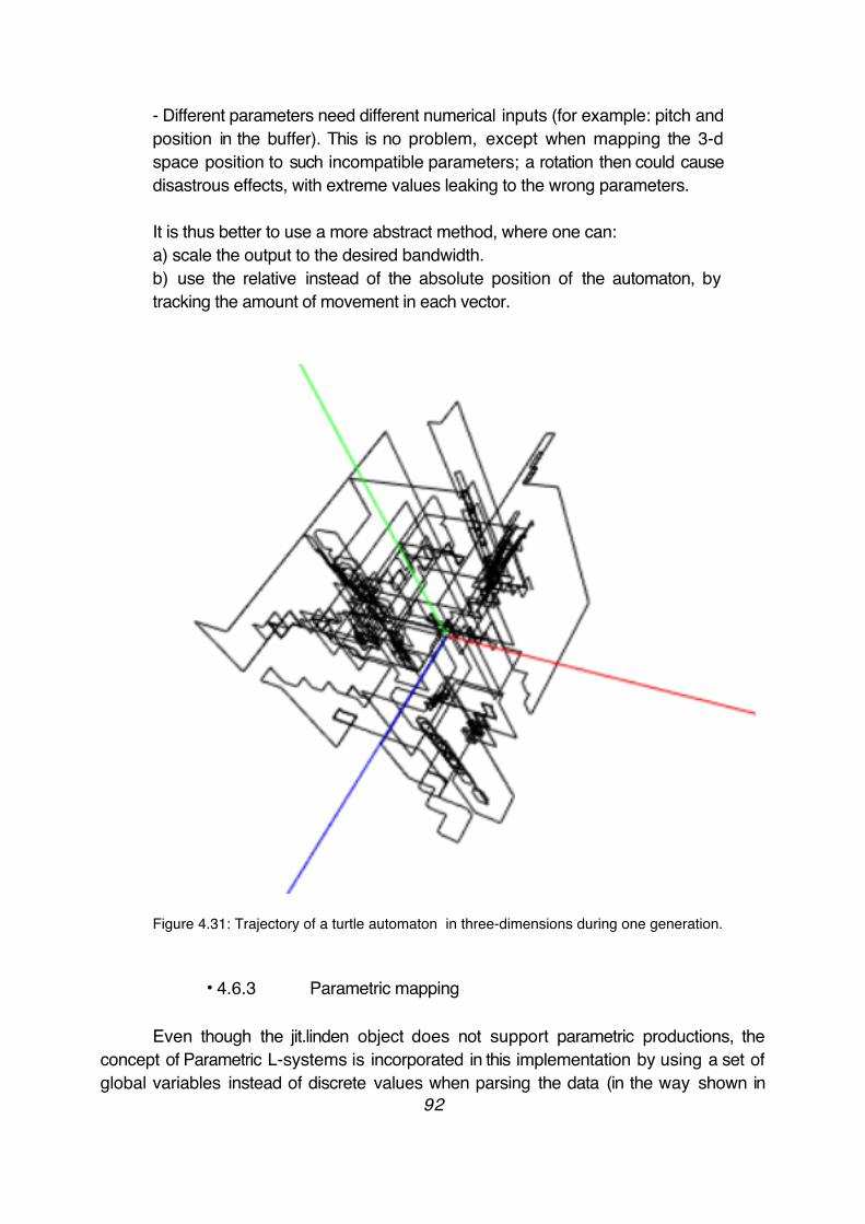
- Different parameters need different numerical inputs (for example: pitch and position in the buffer). This is no problem, except when mapping the 3-d space position to such incompatible parameters; a rotation then could cause disastrous effects, with extreme values leaking to the wrong parameters.
It is thus better to use a more abstract method, where one can:a) scale the output to the desired bandwidth.b) use the relative instead of the absolute position of the automaton, by tracking the amount of movement in each vector.
Figure 4.31: Trajectory of a turtle automaton in three-dimensions during one generation.
• 4.6.3 Parametric mapping
Even though the jit.linden object does not support parametric productions, the concept of Parametric L-systems is incorporated in this implementation by using a set of global variables instead of discrete values when parsing the data (in the way shown in
92
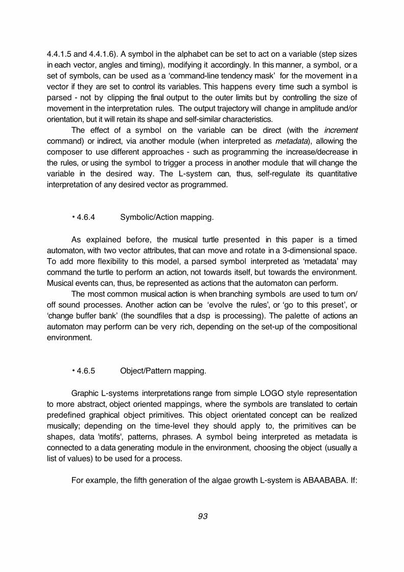
4.4.1.5 and 4.4.1.6). A symbol in the alphabet can be set to act on a variable (step sizes in each vector, angles and timing), modifying it accordingly. In this manner, a symbol, or a set of symbols, can be used as a ‘command-line tendency mask’ for the movement in a vector if they are set to control its variables. This happens every time such a symbol is parsed - not by clipping the final output to the outer limits but by controlling the size of movement in the interpretation rules. The output trajectory will change in amplitude and/or orientation, but it will retain its shape and self-similar characteristics.
The effect of a symbol on the variable can be direct (with the increment command) or indirect, via another module (when interpreted as metadata), allowing the composer to use different approaches - such as programming the increase/decrease in the rules, or using the symbol to trigger a process in another module that will change the variable in the desired way. The L-system can, thus, self-regulate its quantitative interpretation of any desired vector as programmed.
• 4.6.4 Symbolic/Action mapping.
As explained before, the musical turtle presented in this paper is a timed automaton, with two vector attributes, that can move and rotate in a 3-dimensional space. To add more flexibility to this model, a parsed symbol interpreted as ‘metadata’ may command the turtle to perform an action, not towards itself, but towards the environment. Musical events can, thus, be represented as actions that the automaton can perform.
The most common musical action is when branching symbols are used to turn on/ off sound processes. Another action can be ‘evolve the rules’, or ‘go to this preset’, or ‘change buffer bank’ (the soundfiles that a dsp is processing). The palette of actions an automaton may perform can be very rich, depending on the set-up of the compositional environment.
• 4.6.5 Object/Pattern mapping.
Graphic L-systems interpretations range from simple LOGO style representation to more abstract, object oriented mappings, where the symbols are translated to certain predefined graphical object primitives. This object orientated concept can be realized musically; depending on the time-level they should apply to, the primitives can be shapes, data 'motifs', patterns, phrases. A symbol being interpreted as metadata is connected to a data generating module in the environment, choosing the object (usually a list of values) to be used for a process.
For example, the fifth generation of the algae growth L-system is ABAABABA. If:
93
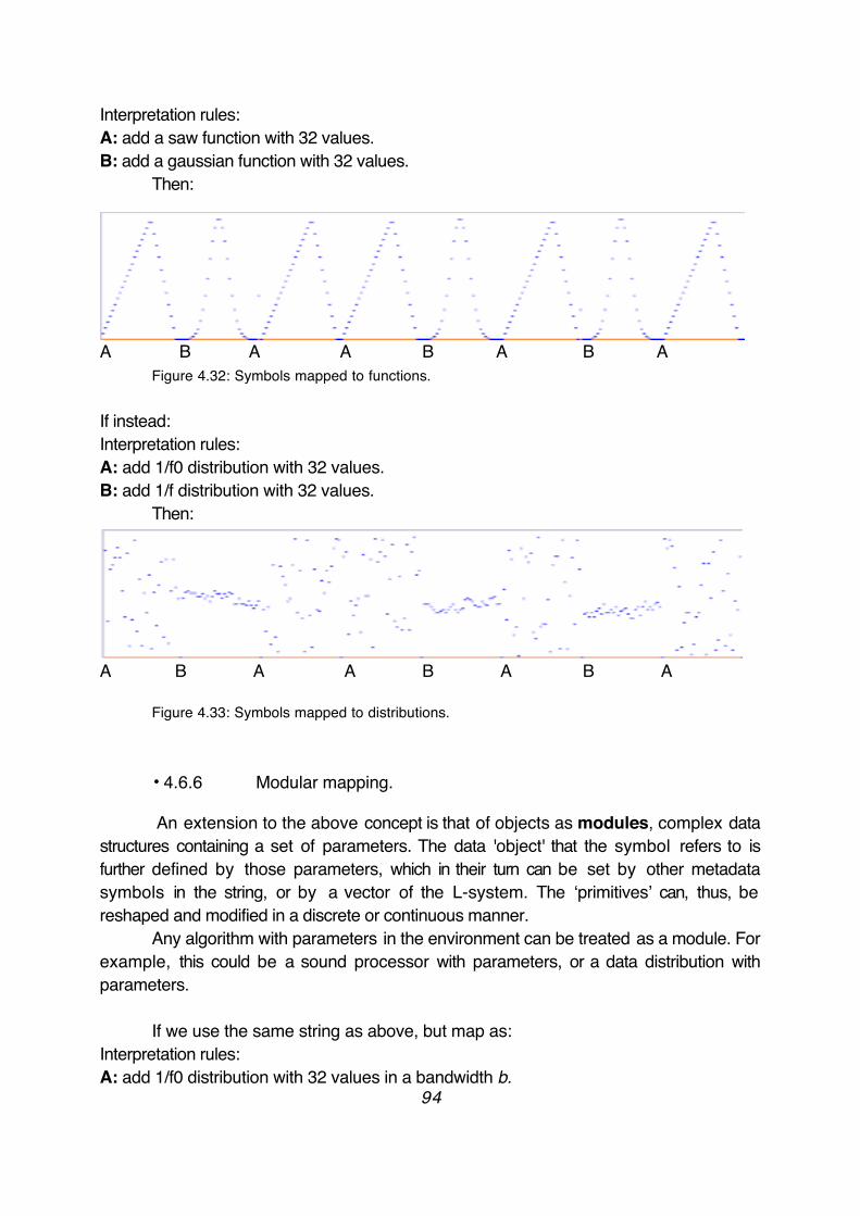
Interpretation rules:A: add a saw function with 32 values.B: add a gaussian function with 32 values.
Then:
A B A A B A B AFigure 4.32: Symbols mapped to functions.
If instead:Interpretation rules:A: add 1/f0 distribution with 32 values.B: add 1/f distribution with 32 values.
Then:
A B A A B A B A
Figure 4.33: Symbols mapped to distributions.
• 4.6.6 Modular mapping.
An extension to the above concept is that of objects as modules, complex data structures containing a set of parameters. The data 'object' that the symbol refers to is further defined by those parameters, which in their turn can be set by other metadata symbols in the string, or by a vector of the L-system. The ‘primitives’ can, thus, be reshaped and modified in a discrete or continuous manner.
Any algorithm with parameters in the environment can be treated as a module. For example, this could be a sound processor with parameters, or a data distribution with parameters.
If we use the same string as above, but map as:Interpretation rules:A: add 1/f0 distribution with 32 values in a bandwidth b.
94
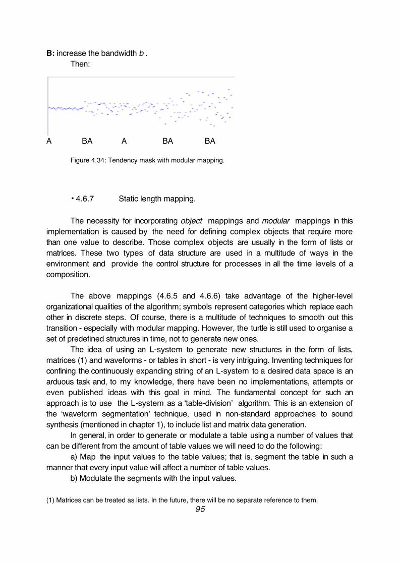
B: increase the bandwidth b .Then:
A BA A BA BA
Figure 4.34: Tendency mask with modular mapping.
• 4.6.7 Static length mapping.
The necessity for incorporating object mappings and modular mappings in this implementation is caused by the need for defining complex objects that require more than one value to describe. Those complex objects are usually in the form of lists or matrices. These two types of data structure are used in a multitude of ways in the environment and provide the control structure for processes in all the time levels of a composition.
The above mappings (4.6.5 and 4.6.6) take advantage of the higher-level organizational qualities of the algorithm; symbols represent categories which replace each other in discrete steps. Of course, there is a multitude of techniques to smooth out this transition - especially with modular mapping. However, the turtle is still used to organise a set of predefined structures in time, not to generate new ones.
The idea of using an L-system to generate new structures in the form of lists, matrices (1) and waveforms - or tables in short - is very intriguing. Inventing techniques for confining the continuously expanding string of an L-system to a desired data space is an arduous task and, to my knowledge, there have been no implementations, attempts or even published ideas with this goal in mind. The fundamental concept for such an approach is to use the L-system as a ‘table-division’ algorithm. This is an extension of the ‘waveform segmentation’ technique, used in non-standard approaches to sound synthesis (mentioned in chapter 1), to include list and matrix data generation.
In general, in order to generate or modulate a table using a number of values that can be different from the amount of table values we will need to do the following:
a) Map the input values to the table values; that is, segment the table in such a manner that every input value will affect a number of table values.
b) Modulate the segments with the input values.
(1) Matrices can be treated as lists. In the future, there will be no separate reference to them.95

The technique used for modulating a given number of table values that is larger than the number of input values is interpolation. This is a widely used function in the compositional environment presented in this thesis, used in several data and audio processing modules. There are five interpolation possibilities:
1. Defined interpolation; Interpolate with a table (the default is linear interpolation). The values in the table can be defined manually, or via a module.
2. ‘Fractal’ interpolation; the overall shape of the table will be used as the interpolation shape between two points in the table.
3. Random interpolation. Interpolate randomly.4. Loop; no interpolation. The total shape is repeated a number of times in
sequence until the table length is filled with values.5. Bypass; no interpolation. Each point is repeated a number of times in order to
scale the shape to the table length.
a) Defined interpolation: linear b) Defined interpolation: triangle
c) Fractal interpolation d) Random interpolation
e) No interpolation: loop f) No interpolation: bypass
Figure 4.35: Different types of interpolation.
96

• 4.6.7.1. Non-Propagative systems: Cellular automata with L-systems.
The most obvious way for confining the output of an L-system to a desired length is by using Non-Propagative L-systems. These types of L-systems can be used as cellular automata algorithms. This is suggested by the similarities between the two systems. As shown in [Alfonseca-Ortega, 1998]:
• Both have initial information that can be considered as their starting state. - For an L-system, the initial string (the axiom). - For a cellular automaton, the set of all the initial states of its finite automata, which can be considered the initial state of the cellular automaton.
• Both have components that record the way the system changes: - For an L-system, the set of production rules. - For a cellular automaton, the transition function of its finite automata.
• Both architectures generate the next state by applying the transformation to every component in parallel.
- The L-System changes each symbol of the current string - The cellular automaton changes the state of each automaton in the grid.
In this paper, the authors demonstrate how a non-propagative, context-sensitive parametric L-system can produce the same results as an n-dimensional cellular automaton. Nevertheless, the limitation of the 'jit.linden' object to only 50 non-parametric production rules allows only for 1-dimensional cellular automata (with two neighbours) with up to three different states (that is 27 rules; four states would require 64 rules).
Cellular automata are possibly one of the most widely used biology-inspired complex systems for electronic music. There is a lengthy bibliography with various suggestions about how to interpret them musically. Various computer music applications using cellular automata exist, such as Chaosynth, CAMUS, Peter Beyls’ modular LISP program and Alik’ s Tehis.
The parsing method for Non-Propagative L-systems differs from that used for Propagative systems. A symbol in the string does not represent an instruction for a turtle automaton, but the current state of a cell. As such, instead of linearly interpreting the string of each generation in a number of steps , the entire production is parsed simultaneously and at once.
The output is a 1-dimensional string. Usually, symbols are translated into values, 97
representing the state of a cell. The concept is based on the standard cellular automata interpretations, e.g. in the grammar shown in chapter 2.5.7, symbols A and B correspond to 0 and 1 respectively. A table can be used to alter this interpretation (then A=1 and B=0). Symbols are treated as values also when setting the axiom and the production rules. This allows for a more compact visualization and, most importantly, using numerical functions to provide the axiom and the rules.
As an outcome to that, the axiom, the production rules and the interpretation rules can be provided in the following ways:
1. randomly (internal).2. manually.3. with a function/ list sent from another module.The third option allows linking the system to a list parameter in the compositional
environment. While using a parameter as an axiom, the state of the system will change if that parameter changes from outside the L-system, feeding back to the parameter the new state.
Control mechanisms, as presented in chapter 4.5, can be used to change the rules. This includes using sets of rules stored in tables, evolving rules with genetic algorithms and using hierarchical networks of L-systems. Wolfram’ s categorization of cellular automata rules can be a basic framework for finding a production rule with a desired behaviour:
1. Rules pushing fast to a steady state.2. Rules producing cyclic transitions with periods of variable length.3. Rules generating complex and localized structures.4. Rules determining chaotic behavior.
Several types of mappings are used in this implementation, some incorporating already existing ideas and some new ones, that were allowed and dictated by the overall structure of the program. The mapping schemes used here are:
1. Send the entire generation as a list (or matrix).2. Split the list into groups and send each group separately.3. Split into individual cells and send each separately.4. Interpolate or extrapolate to a desired cell space (list length) and send the new list. The grid - or number of cells - of the automata affects greatly the output of the algorithm. The smaller the grid is, the faster a state will reverberate, meaning that it will reach the edge of the cell grid and bounce back. Interpolation and extrapolation give the possibility to experiment with the reverberations of different cell spaces (cell grids), even when the output list needs to be of a certain length. Interpolation and extrapolation can also be used to change the resolution of the output list - meaning the amount of different states.
98
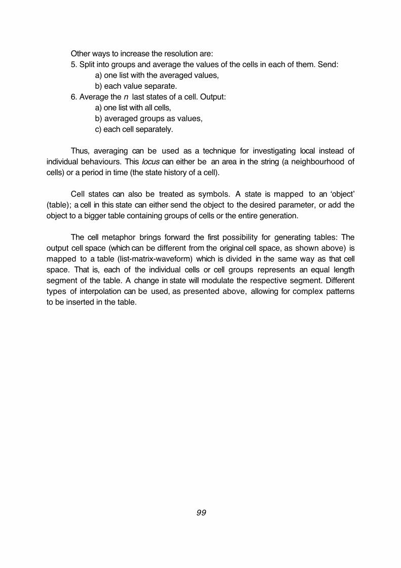
Other ways to increase the resolution are:5. Split into groups and average the values of the cells in each of them. Send:
a) one list with the averaged values, b) each value separate.
6. Average the n last states of a cell. Output:a) one list with all cells,b) averaged groups as values, c) each cell separately.
Thus, averaging can be used as a technique for investigating local instead of individual behaviours. This locus can either be an area in the string (a neighbourhood of cells) or a period in time (the state history of a cell).
Cell states can also be treated as symbols. A state is mapped to an ‘object’ (table); a cell in this state can either send the object to the desired parameter, or add the object to a bigger table containing groups of cells or the entire generation.
The cell metaphor brings forward the first possibility for generating tables: The output cell space (which can be different from the original cell space, as shown above) is mapped to a table (list-matrix-waveform) which is divided in the same way as that cell space. That is, each of the individual cells or cell groups represents an equal length segment of the table. A change in state will modulate the respective segment. Different types of interpolation can be used, as presented above, allowing for complex patterns to be inserted in the table.
99
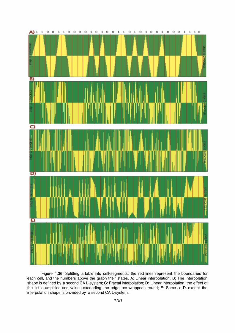
Figure 4.36: Splitting a table into cell-segments; the red lines represent the boundaries for each cell, and the numbers above the graph their states. A: Linear interpolation; B: The interpolation shape is defined by a second CA L-system; C: Fractal interpolation; D: Linear interpolation, the effect of the list is amplified and values exceeding the edge are wrapped around; E: Same as D, except the interpolation shape is provided by a second CA L-system.
100

• 4.6.7.2. Generating waveforms and lists with bracketed L-systems.
However interesting a cellular automata model might be, there are a number of disadvantages to it when compared to the interpretations of Propagative L-systems proposed above. Cellular automata are categorical. A cell can be in one state or the other, not in between. The turtle automaton implemented here is much more versatile, being able to move in a five-dimensional float number space and perform actions. Apart from high resolution and multidimensionality, the timing interpretation is also much more interesting; in cellular automata all the cells change state simultaneously, whereas branched automata can control their own parsing speed.
The same method for segmenting a table as for cellular automata can also be used for Bracketed L-systems. The actual branches found in the string are grouped, stochastically or with maximum overlap, to a given number of output branches representing data voices, in the manner explained in chapter 4.4.1.5. A branched automaton group can be treated as a cell/segment, containing up to five dimensions and having its own timing. A separate table is produced for every vector, consisting of the values of each output branch in the respective vector. This is a parallel processing model; each cell works autonomously on the output level. Hierarchical connections and branching structures have an indisputable effect on the actual values of the table but the actual relations become obscure during the grouping process.
101
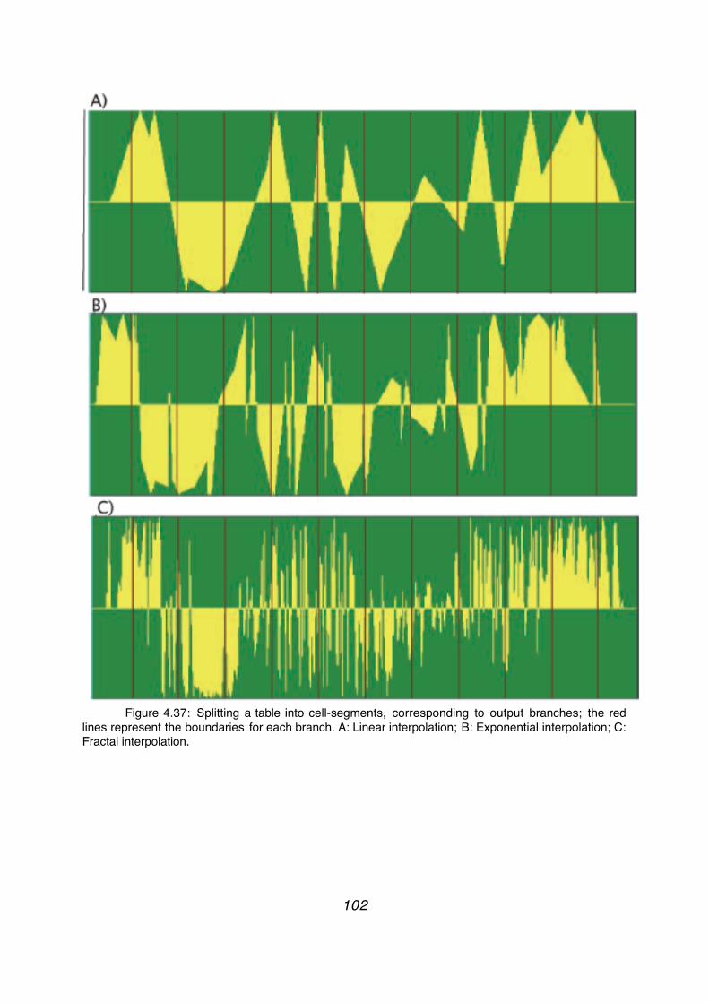
Figure 4.37: Splitting a table into cell-segments, corresponding to output branches; the red lines represent the boundaries for each branch. A: Linear interpolation; B: Exponential interpolation; C: Fractal interpolation.
102
It is possible to use the branching structure of a bracketed L-system to segment the table hierarchically. In general, in order to parse a bracketed L-system, a map has to be made for every generation, carrying information about the tree, each branch and the branching structure and hierarchies. Some of this information can also be used for making table interpretations:
a) how many 1st order branches exist in the current generation of the tree.b) of which depth level (order) is a branch - meaning, how many branches it is away from the trunk.c) which is the parent branch of a sub-branch. d) what is the (local) index of the parent branch in its own parent branch - meaning, how many branches of the same level will the (grand)parent generate before it generates the parent .e) how many sub-branches of the same level (or 'siblings') does the parent of a branch contain.f) what is the local index of a branch - meaning, how many branches of the same level will the parent generate before it generates this branch.
One way to incorporate the layer specific hierarchical aspects of a bracketed L-system is by extending the concept of defined interpolation. The depth-level of a branch represents its hierarchical importance in the current generation. Branches closer to the trunk are considered to be more important than others further away. Instead of using a function or another L-system to define the interpolation shape we can group all the branches of a certain depth level in a table representing the interpolation layer that determines the shape between values of the superordinate depth level. The first level branches form the initial highest order list whereas the trunk can be used as a multiplier for determining the overall effect of the branch movement in the list. For example, see figure 4.31. Apart from the interpolated table for the entire system, each depth level table can be sent as a control for any process in the environment.
103
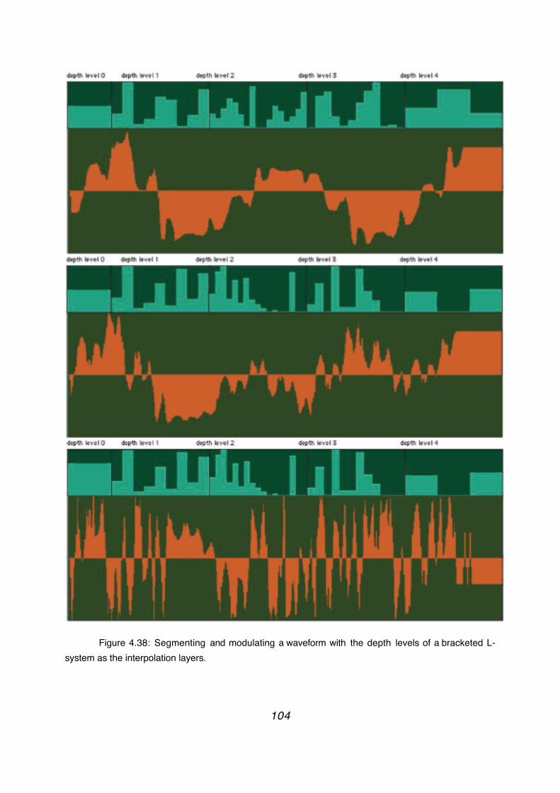
Figure 4.38: Segmenting and modulating a waveform with the depth levels of a bracketed L-system as the interpolation layers.
104
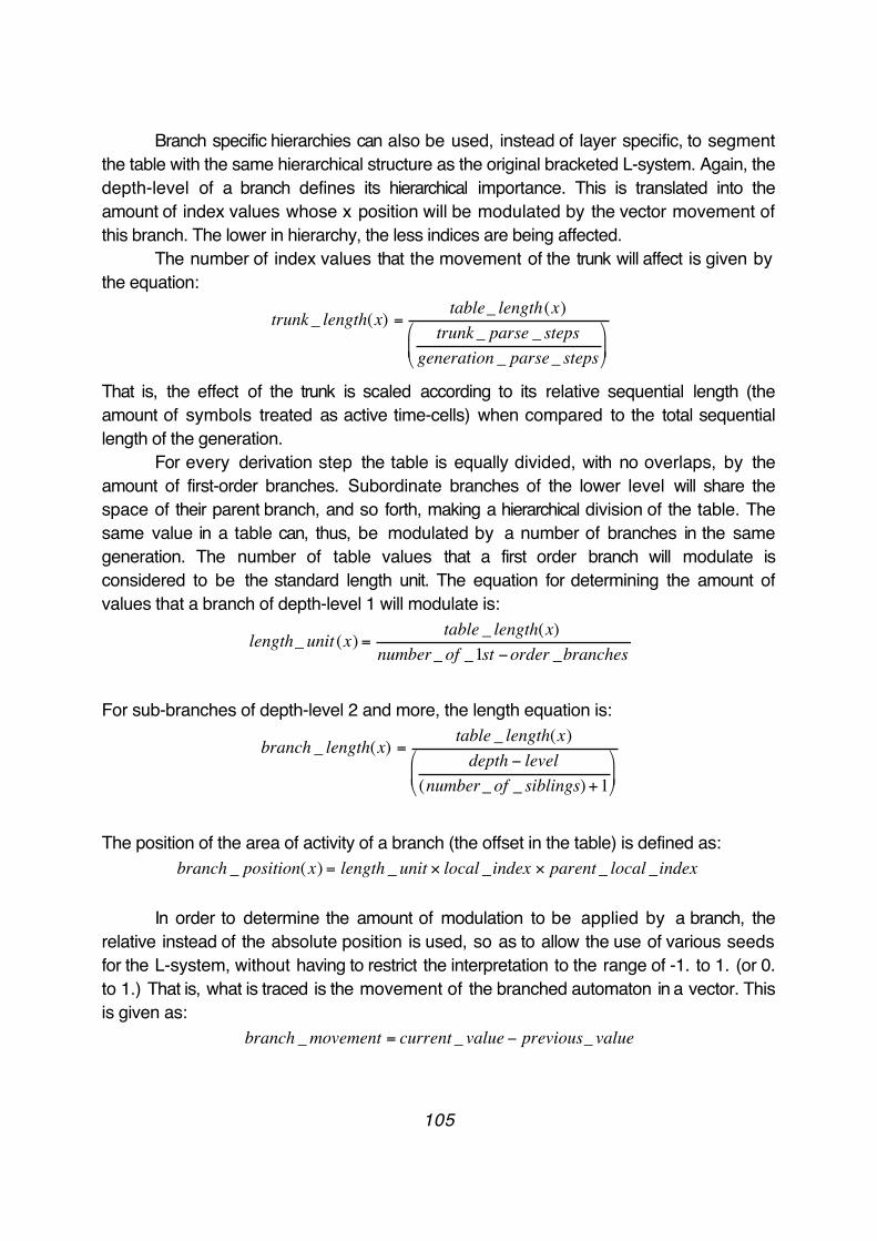
Branch specific hierarchies can also be used, instead of layer specific, to segment the table with the same hierarchical structure as the original bracketed L-system. Again, the depth-level of a branch defines its hierarchical importance. This is translated into the amount of index values whose x position will be modulated by the vector movement of this branch. The lower in hierarchy, the less indices are being affected.
The number of index values that the movement of the trunk will affect is given by the equation:
€
trunk_ length(x) =table_ length(x)
trunk_ parse _ stepsgeneration _ parse_ steps
That is, the effect of the trunk is scaled according to its relative sequential length (the amount of symbols treated as active time-cells) when compared to the total sequential length of the generation.
For every derivation step the table is equally divided, with no overlaps, by the amount of first-order branches. Subordinate branches of the lower level will share the space of their parent branch, and so forth, making a hierarchical division of the table. The same value in a table can, thus, be modulated by a number of branches in the same generation. The number of table values that a first order branch will modulate is considered to be the standard length unit. The equation for determining the amount of values that a branch of depth-level 1 will modulate is:
€
length_ unit (x) =table _ length(x)
number_ of _1st −order _branches
For sub-branches of depth-level 2 and more, the length equation is:
€
branch _ length(x) =table _ length(x)depth − level
(number_ of _ siblings) +1
The position of the area of activity of a branch (the offset in the table) is defined as:
€
branch _ position(x) = length _ unit × local _index × parent_ local _index
In order to determine the amount of modulation to be applied by a branch, the relative instead of the absolute position is used, so as to allow the use of various seeds for the L-system, without having to restrict the interpretation to the range of -1. to 1. (or 0. to 1.) That is, what is traced is the movement of the branched automaton in a vector. This is given as:
€
branch _movement = current_ value − previous_ value
105
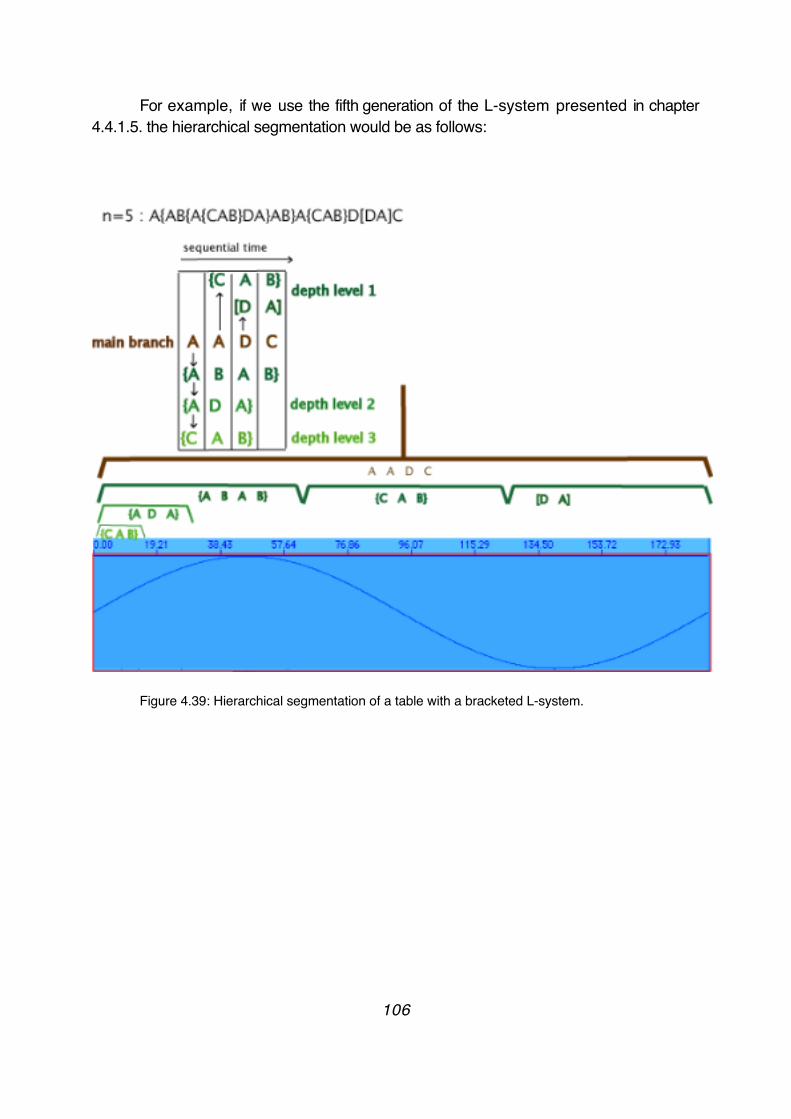
For example, if we use the fifth generation of the L-system presented in chapter 4.4.1.5. the hierarchical segmentation would be as follows:
Figure 4.39: Hierarchical segmentation of a table with a bracketed L-system.
106
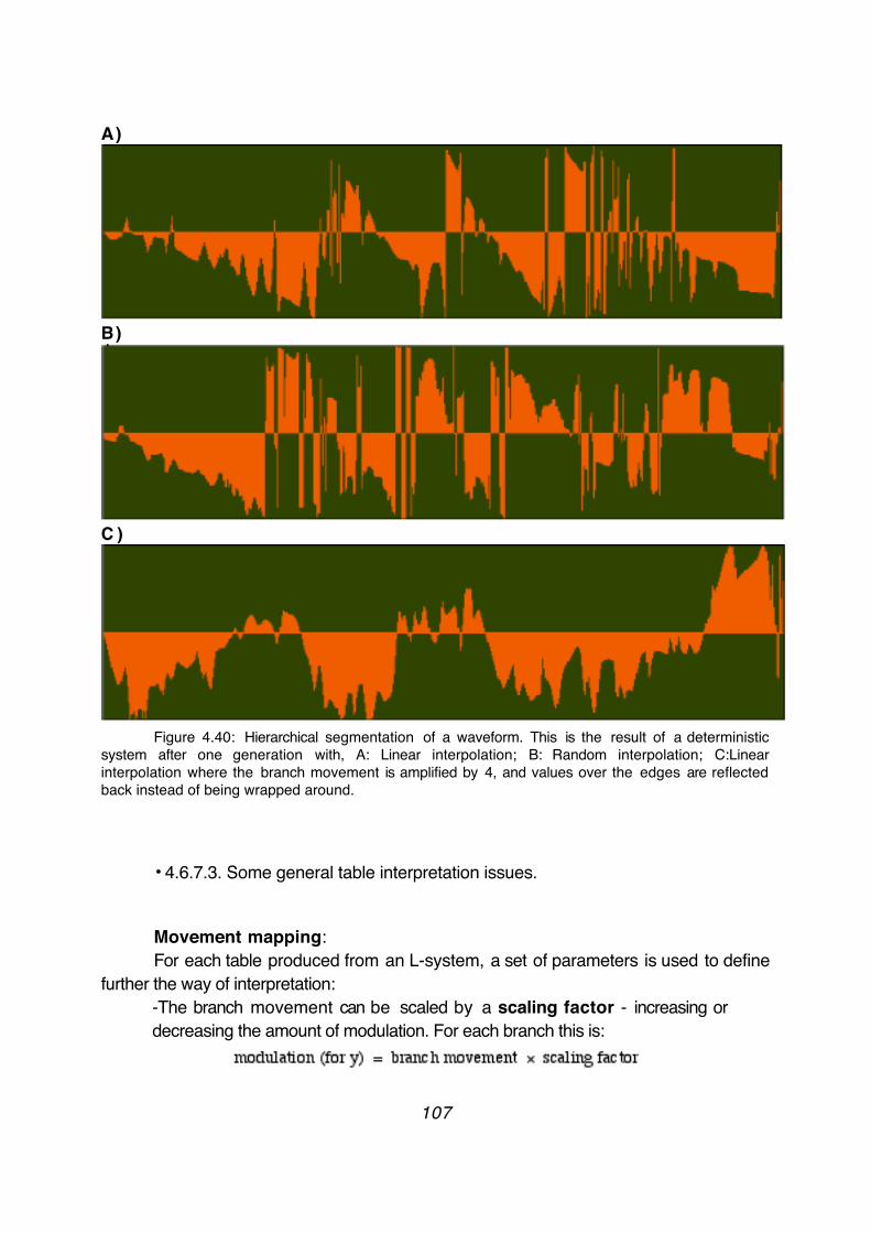
A)
B)
C )
Figure 4.40: Hierarchical segmentation of a waveform. This is the result of a deterministic system after one generation with, A: Linear interpolation; B: Random interpolation; C:Linear interpolation where the branch movement is amplified by 4, and values over the edges are reflected back instead of being wrapped around.
• 4.6.7.3. Some general table interpretation issues.
Movement mapping:For each table produced from an L-system, a set of parameters is used to define
further the way of interpretation:-The branch movement can be scaled by a scaling factor - increasing or decreasing the amount of modulation. For each branch this is:
107
-A clipping function is used when a value exceeds the range of the table. There are three options:
1. Clip; the value is clipped to the range.2. Reflect; the value is reflected back. (similar to GenDy’ s elastic barriers)3. Wrap; the value is wrapped to the other end.
- The interpolation type needs also to be specified, in the case that the table consists of more values than the input values.
Seeding:The table interpretation of the movement of an L-system is iterative. This allows
for seeding the table with a list, matrix or waveform external from the L-system. In this way, the L-system grabs the state of the controlled table and modulates it according to the amount of branched movement on the controlling vector, transforming the given structure. If no seed is provided, modulation starts from zero (or a void state) and the L-system generates new data from an empty structure.
Incorporating object mapping:A table generating technique based on the turtle movement can be combined
with other types of mappings. A symbol in the alphabet can be interpreted as a command to insert an ‘object’ in the table (function/shape/distribution). When such a symbol is found in a branch, the object will be inserted in the respective area of activity of that branch in the table.
Incorporating modular mapping:Modular mapping can be used to insert a predefined type of object in a branch
table-space, with parameters that define its actual shape.
• 4.7 Controller outputs and control modes: summary.
The data produced by the L-systems are interpreted and then sent as controllers to the compositional environment. The number of control channel outputs depends on the type and interpretation of the system.
Values:A non-branched L-system produces a single stream of data flow or a single turtle
automaton. A branched L-system, on the other hand, produces a hierarchical network of turtle automata. The state of each automaton, defined as the vector set: {x, y, z, roll, yaw, pitch, thik, colr, time} is output on a different channel for each vector. The amount of vectors that will change in time is defined in the interpretation rules, by setting symbols to change the state of the automaton in this or the other vector. Rotations in x, y, z, will cause
108
movement in a combination of these vectors, even if only forward movement towards the direction that the turtle faces is programmed. Mapping can be absolute or iterative and it is possible to send the same data to a number of parameters. Iterative mapping is, naturally, more powerful, translating the L-system into a contour trajectory description method that is decoupled from the actual values of the receiving parameter. The output values can be separately scaled and clipped (clip, reflect, wrap) for each parameter. Techniques for limiting the data voices of a branched L-system were explained in chapter 4.4.1.5.
Commands/ actions:In addition to the automaton state, turtle actions - metadata symbols - are also
output in a separate channel for each symbol. For branched systems, a metadata symbol will be sent separately for every branch and, as well, through a reserved channel including all branches - all occurrences of the symbol in a generation will be output from there. Branching symbols are also output as metadata.
Lists:For each vector of the L-system a list is output representing the current state of the
entire system as shown in 4.6.7. In addition, a separate list for the current state of each depth-level for every vector is also output. The interpretation is iterative, using a defined or an empty seed list. Lists can also be translated into matrices.
Waveforms:As mentioned before, the current state of each vector and the current state of each
depth-level of an L-system - Bracketed or Non-Propagative - can be iteratively linked to an existing or empty waveform.
109
▼ Chapter 5: Compositional strategies.
The fundamental assumption in this thesis is that a musical form or behavior can be modelled as a complex dynamic system with dynamic structure that develops over time. L-systems provide a very useful and compact abstract method and computational framework for this purpose. In order to design such a system, we first have to divide it in its basic components. That is:
a) The field: This is the compositional parameter space with its grids/reference frames for each vector. The compositional space need not be a Euclidean space; instead, we can use an abstract hierarchical space, where a dimension may contain a set of subordinate dimensions or even subordinate systems. Movement can then be organized hierarchically in different levels; this is particularly useful, in order to be able to effectively compose in the perceptual space of sound, using embedded processes to interpolate to the instrument space of the DSPs. b) The movement: This is the trajectory of the system in the compositional phase space (in the field).c) The control mechanisms: These are mechanisms that transform the field and the type of movement in time.d) The time organization: Subsequently, we will need to organize all of the above in time. It can be useful to extend the hierarchical space concept to include time-level hierarchies. The composer can then design each level separately and take different compositional approaches in the overall design: top-down, bottom-up, middle-out or hybrid.
The power of the L-system model proposed in this thesis lies in its flexibility in designing and carrying out various complex and dynamic models and its ability to act upon all of the basic components listed above. A musical turtle can generate trajectories in time in a multi-dimensional phase space, and also act upon itself, its field and the compositional environment as a control mechanism. Multiple automata and multiple L-systems can be active at the same time, defining different aspects of the composition. The complexity of the possible applications depends only on the processing power of our computers and on our ability to conceptualize.
In the following chapter, I will introduce some ideas for using L-systems to compose in different time-levels. In parallel, I will give some audio examples, following a bottom-up approach for designing a musical form, starting from the sample level and proceeding upwards, for the sake of clarity.
110
• 5.1. Composing in different time levels.
• 5.1.1. Sample level:
As mentioned before, Non-Propagative and Bracketed L-systems can be used to create or transform waveforms in the sample level. Since a single sample has no perceptual quality, L-systems are used as a waveform segmentation technique for generating musical quanta with certain characteristics. This is a twofold process, and one has to decide on:
1. How to segment the waveform.2. How to modulate the waveform.
The L-system model presented above provides a very powerful and versatile model for both. The segmentation can be:
a) Parallel and without overlaps. We can call this the "cell model": the waveform is divided into a number of equal length segments, each being modulated by a cell or cell-group (for Non-Propagative L-systems, see chapter 4.6.7.1), or by a branch-group (for Bracketed L-systems when the real branches generated from the system are either mapped to an arbitrary number of output branches, or grouped by level of hierarchy, see chapters 4.4.1.5 and 4.6.7.2.). In order to change the number of segments one has to change the number of assigned output cells or branches.b) Depth level segmentation. We can call this the “layer model”. The branches of a Bracketed L-system are grouped into depth levels, which are used as interpolation layers for generating larger tables. The segmentation will dynamically change after each derivation step, following the depth level structure of the tree. c) Hierarchical segmentation. We can call this the "tree model": the structure of a Bracketed L-system is used to divide the waveform hierarchically. Each brach generated from the system ('real branch') will modulate a certain number of samples, their amount depending on the level of hierarchy of the branch in the tree, and their position in the waveform depending on its position in the overall tree structure (again, see chapter 4.6.7.2). The segmentation will dynamically change after each production, following the structure of the tree.
Each segment will be modulated in one or both of the following methods:a) The "object method". A function or a distribution can be inserted in the segment (with object or modular mapping, see chapters 4.6.5 and 4.6.6)b) The "movement method". The existing sample values of the segment can be iteratively modulated with the movement value of the controlling
111
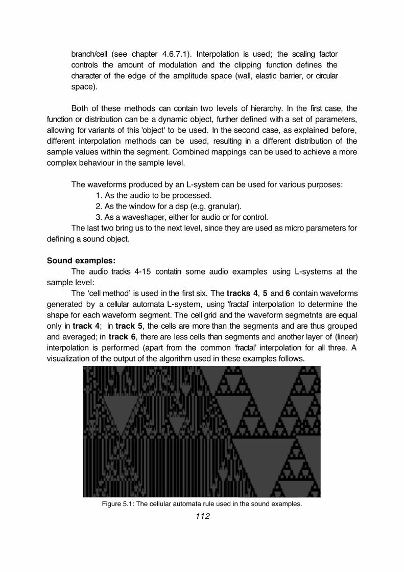
branch/cell (see chapter 4.6.7.1). Interpolation is used; the scaling factor controls the amount of modulation and the clipping function defines the character of the edge of the amplitude space (wall, elastic barrier, or circular space).
Both of these methods can contain two levels of hierarchy. In the first case, the function or distribution can be a dynamic object, further defined with a set of parameters, allowing for variants of this 'object' to be used. In the second case, as explained before, different interpolation methods can be used, resulting in a different distribution of the sample values within the segment. Combined mappings can be used to achieve a more complex behaviour in the sample level.
The waveforms produced by an L-system can be used for various purposes: 1. As the audio to be processed.2. As the window for a dsp (e.g. granular).3. As a waveshaper, either for audio or for control.
The last two bring us to the next level, since they are used as micro parameters for defining a sound object.
Sound examples:The audio tracks 4-15 contatin some audio examples using L-systems at the
sample level: The ‘cell method’ is used in the first six. The tracks 4, 5 and 6 contain waveforms
generated by a cellular automata L-system, using ‘fractal’ interpolation to determine the shape for each waveform segment. The cell grid and the waveform segmetnts are equal only in track 4; in track 5, the cells are more than the segments and are thus grouped and averaged; in track 6, there are less cells than segments and another layer of (linear) interpolation is performed (apart from the common ‘fractal’ interpolation for all three. A visualization of the output of the algorithm used in these examples follows.
Figure 5.1: The cellular automata rule used in the sound examples.
112
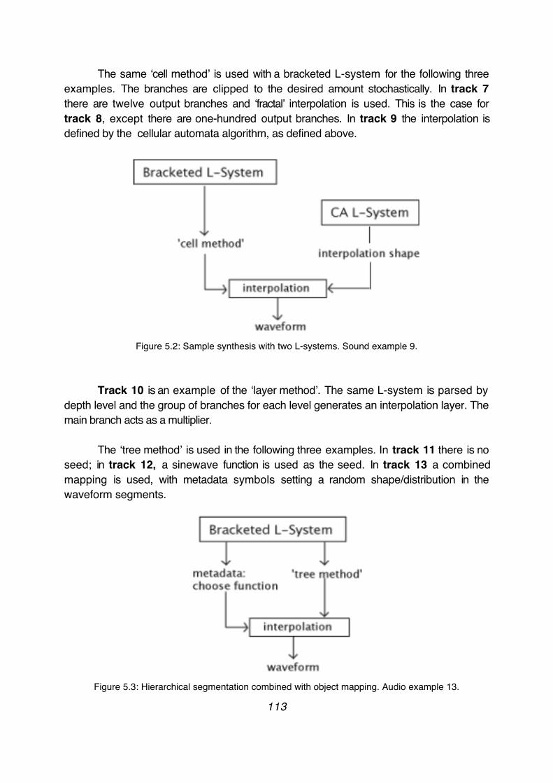
The same ‘cell method’ is used with a bracketed L-system for the following three examples. The branches are clipped to the desired amount stochastically. In track 7 there are twelve output branches and ‘fractal’ interpolation is used. This is the case for track 8, except there are one-hundred output branches. In track 9 the interpolation is defined by the cellular automata algorithm, as defined above.
Figure 5.2: Sample synthesis with two L-systems. Sound example 9.
Track 10 is an example of the ‘layer method’. The same L-system is parsed by depth level and the group of branches for each level generates an interpolation layer. The main branch acts as a multiplier.
The ‘tree method’ is used in the following three examples. In track 11 there is no seed; in track 12, a sinewave function is used as the seed. In track 13 a combined mapping is used, with metadata symbols setting a random shape/distribution in the waveform segments.
Figure 5.3: Hierarchical segmentation combined with object mapping. Audio example 13.
113
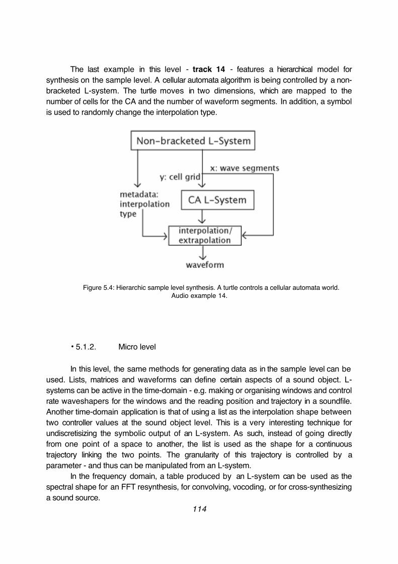
The last example in this level - track 14 - features a hierarchical model for synthesis on the sample level. A cellular automata algorithm is being controlled by a non-bracketed L-system. The turtle moves in two dimensions, which are mapped to the number of cells for the CA and the number of waveform segments. In addition, a symbol is used to randomly change the interpolation type.
Figure 5.4: Hierarchic sample level synthesis. A turtle controls a cellular automata world. Audio example 14.
• 5.1.2. Micro level
In this level, the same methods for generating data as in the sample level can be used. Lists, matrices and waveforms can define certain aspects of a sound object. L-systems can be active in the time-domain - e.g. making or organising windows and control rate waveshapers for the windows and the reading position and trajectory in a soundfile. Another time-domain application is that of using a list as the interpolation shape between two controller values at the sound object level. This is a very interesting technique for undiscretisizing the symbolic output of an L-system. As such, instead of going directly from one point of a space to another, the list is used as the shape for a continuous trajectory linking the two points. The granularity of this trajectory is controlled by a parameter - and thus can be manipulated from an L-system.
In the frequency domain, a table produced by an L-system can be used as the spectral shape for an FFT resynthesis, for convolving, vocoding, or for cross-synthesizing a sound source.
114

Sound examples:The same bracketed L-system used in the above chapter is used in the following
three sound examples for frequency domain timbral tranformations. In track 15 it is used for convoluting a vocal sample. The same sample is being vocoded with the L-systems output in track 16 and cross-synthesized in track 17.
Going back to the time domain, the ‘layer method’ is used in track 18 to generate the window for a granular process. The soundfile used is another vocal sample. It should be mentioned that, for all the examples given here, there is no data activity in higher levels than the one presented - all the parameters of the synthesis engine remain static and only the sample values of the required buffers for the granular synthesis(window, soundfile and reading shape) are being modified by the L-systems. In track 19, L-systems are used to generate the window for a granular process, as well as a waveshaper, to control the reading position in the soundfile (voice sample).
A combination of L-systems is used in the next example, track 20. A bracketed L-system produces the soundfile and the window for a granular process, while the main branch controls a CA L-system in the same manner as for track 14.
Figure 5.5: Hierarchic sample level synthesis. An L-system produces the waveform and the window while controling another L-system that performs waveshaping on the window. Audio example 20.
• 5.1.3. Sound object
This level is an extended equivalent of the traditional note-level. L-system implementations for music have mainly dealt with this level. However, due to the fundamentally different concepts of traditional and electronic music, this level has to be redefined.
Notes represent discrete semantic states in the phase space of a musical system. Notes are 'homogenous' [Roads, 2001] and static; their meaning and function is given by
115

their (discrete) position in the multi-dimensional perceptual space. In electronic music, however, the semantic weight of a sound object lies not in the static state it represents, but more often in the ways it moves from one point of the perceptual space to the other. A sound object is thus a collection of characteristics and properties of the micro- level that form a sonic unit.
To simplify things, we can borrow the concept of "stasis" and apply it to the instrument space instead of the perceptual space. A sound object can thus be defined as a static configuration of a dsp engine - meaning that none of its parameters changes over time - which can be moving in the perceptual space, but only in the manner defined by the current configuration of the parameters.
Discrete mappings can be used to organize different types and properties of sound objects in a sequence provided by the L-system. Such are event-literal mappings, absolute spatial mappings (by tracking not the movement but the absolute position of the automaton in the phase space) and object mappings. These schemes can be used in various manners, retrieving presets, distributions, shapes, parameter values.
• 5.1.4. Meso level
The metaphor of navigation through a compositional space is very useful for composing musical structures in this level. L-systems are very powerful in generating interesting trajectories and it is up to the composer to make an adequate configuration of the compositional field - mapping the vectors of the space and adding a grid. Iterative movement mappings are, by far, more interesting than absolute spatial mappings, grabbing the fractal trajectory character of the interpreted system and using it to model change, regardless of the value and bandwidth of the actual parameter.
'Objects' or 'modules' generated by an L-system can also be treated as shapes and distributions (patterns) that will be sent to sequencer-type modules controlling parameters of a dsp at this time level. A combination of mappings can be used to model behaviours of any desired complexity.
One of the most interesting features of L-systems in this level is their ability to generate multiple data streams with self-similar and 'contrapuntal' behaviour. A Bracketed L-system can produce a multitude of turtle-automata, each one of which is a musical agent, moving and acting. Techniques for obtaining the desired amount of branch automata from an L-system and the way to define the data density of each automaton have already been discussed (chapter 4.4.1.5.)
116

sound examples:Proceeding to the meso level, we can extend the strategy presented above to
include more data layers. A first step is to use the movement of a turtle automaton - the trunk - in a space to iteratively move a defined parameter. As an additional micro- shape, we will add an interpolation layer inbetween the values produced by the turtle, to make its path more continuous. The shape will be taken from the overall state of the L-system. This is the case for track 21, which uses a waveform produced by the L-system, and track 22, which uses a drum loop from the Max/MSP distribution. This strategy expands to include metadata actions for seeding the tables and setting the interpolation type in the following three examples. Track 23 features, again, an L-system generated waveform, while track 24 uses the drum loop. In track 25 the soundfile is a harpsichord recording. The parameter affected in all these examples by the trunk is the grainlength. The general scheme followed in these examples is the following:
Figure 5.6: Fractal interpretation of the movement of a Bracketed L-system in one dimension.
In the above examples, only one dimension of the trunk-turtle movement is used. To clarify the contrapuntal characteristics of a bracketed L-system we will go to track 26. There is no activity in any but the current level; a 3-dimensional branched L-system is mapped to the following parameters of a granular synthesis: grainlength, pitch and reading speed. The real branches are grouped stochastically to a group of eight output branches, each corresponding to a granulator. The soundfile used is a sinewave function. The settings for track 27 are the same, except this time the soundfile is generated in real-time by the L-system. Metadata is also used to set the interpolation type.
117
Simpler strategies can also produce interesting results in this level. In track 28, a turtle automaton is used to navigate in a two dimensional space; the space represents a regular - irregular distribution continuum for the position in the buffer (x) and the reading speed (y). If the turtle is at point zero the distribution of the granulators in these parameters is uniform, otherwise randomness is inserted. All the other granular synthesis parameters remain static.
• 5.1.5. Macro level
The incorporation of several kinds of control mechanisms in this implementation focused on providing a multitude of ways and possible strategies for developing a musical system over time.
All the elements of an L-system may be subjected to change; that is, the production rules, the decomposition and the interpretation rules, the axiom, the seeds, the variables and the mapping. The control mechanisms can either be provided by the L-system itself, with 'parametric' and 'action' mappings, or by an external process (manually or from another module or L-system).
Different strategies may be realized, ranging from the strict determinism of storing rules into presets and recalling them - with Table L-systems - to the biologic conditioned randomness of using genetic algorithms for evolving a grammar or to designing hierarchical connections and interdependencies between systems. There are plenty of possibilities, and the composer may choose which structures he needs to explicitly define and which to stochastically lead into emergence. With a well-planned overall design, it is possible to generate different sets of automated compositions, and different sets of interactive installations with the same set-up.
sound examples:Track 3 is a macroform example of a hierarchical network of non-bracketed L-
systems. A main L-system controls a number of subordinate systems and parameters for granular synthesis, as shown in the following figure. The processed soundfiles are from a harpsichord recording.
118
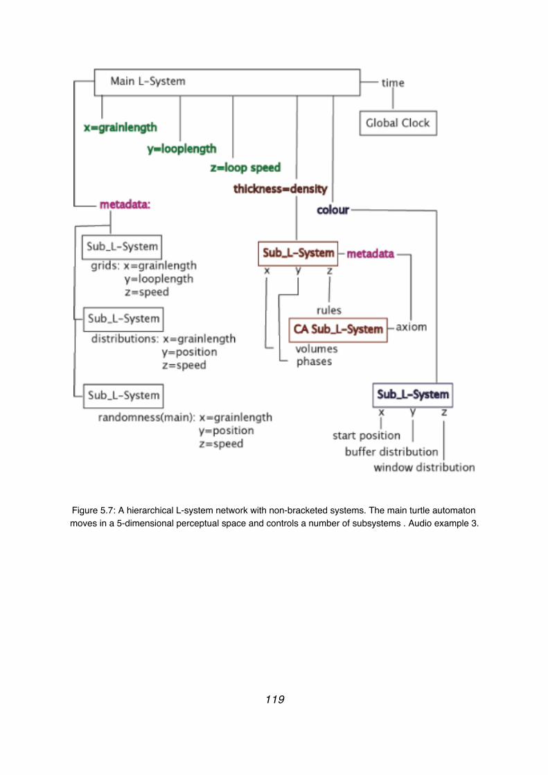
Figure 5.7: A hierarchical L-system network with non-bracketed systems. The main turtle automaton moves in a 5-dimensional perceptual space and controls a number of subsystems . Audio example 3.
119
▼ Chapter 6: Conclusions.
Scientific and technological advancements have always played a major role in the way we perceive, comprehend and organize sound, continuously stretching the field of music. Digitalization has expanded the compositional area into a multitude of levels and layers, allowing and demanding for different strategies to be invented in order to provide sufficient control over the entire compositional procedure.
This thesis proposes that a musical system can be designed as a complex dynamic system with dynamic structure that evolves over time. L-systems, primarily concerned with emergence and morphogenesis, provide a very useful abstraction and computational method for such a task. The compositional field can be thought of as a complex hierarchical space, with time scale hierarchies and perceptual-to-mechanic hierarchies (translating perceptual qualities to instrument parameters). L-systems and L-system networks can be used at any level of the composition to provide a multitude of data structures, ranging from the sample level to macroforms, with very interesting results. The composer can divide the field of activity of the overall musical system into a set of functional components with hierarchical structure that develops over time. Several types of control mechanisms between components can be used, allowing for various approaches to be taken - ranging from traditional compositional strategies to real-time improvisation to automated composition. Sonic behaviour in each level can be composed separately and different paths in designing the total compositional system can be followed, e.g. starting from generating waveforms and going up, or deciding on the macroform and building each subordinate level in sequence, or even designing arbitrarily the parts for which it is easier or necessary to formalize first, and then deciding on the rest of the components of the system.
An important feature of the algorithm, magnified by a modular implementation, is the decoupling of the different levels of definition: the production, the parsing and the mapping. This makes it relatively easy to re-use, re-adjust and 'tune' a system according to the kind of sonic behaviour one wishes to generate with it. The flexibility of the algorithm and the environment allow the composer to provide the palette of actions, the mapping, the number of automata and their relation to each other using a wide variety of methods. Each turtle automaton is a musical agent that performs numerous tasks in time and a given composition may include a varying number of interconnected agents. General types of behaviour for these agents can be programmed in the rules, leading to the emergence of complex multi-dimensional patterns in space-time.
Part of the interest of working with generative algorithms is their inherent data amplification characteristic, producing an infinite series of numbers, or instructions. When working with an algorithm such as L-systems, an unbounded number of results will be
120
produced, their interpretation being limited only by the character of the mapping possibilities. A modular approach, such as the one presented here, augments the possibilities of designing musical L-systems by allowing to develop both the algorithm and the environment in parallel, one to fit the needs of the other.
Although the program in its current state is highly sophisticated, it is the starting framework, and the nature of the implementation leaves many opportunities for further expansion. Main points for future research include incorporating parametric productions and a structural analysis module (performing data compression) that can encode an input into a set of production rules. Naturally, future developments will lead to new strategies and methods not yet considered. Through the expansive possibilities of a modular implementation of L-systems, the program retains a progressive nature that allows itself to evolve continuously as the creator does.
121

▼ Appendix.
Some sound examples:
Track 1: Study for Digital Harpsichord Drumming. This is a piece using a harpsichord recording, performed by the author. L-systems are used in the micro, sound object and meso scales. Premiered in the Sonology discussion concert, April 2006.
Track 2: Voice Particles, for voice and live electronics. This is a live performance with Stephanie Pan, recorded live in concert on May 2006 in Den Haag. In this piece L-systems are used in the micro level.
Track 3: ‘Semi-automated’ sound example. This example was composed in February 2006; the goal was to automate with L-systems as much of the compositional procedure as possible.
Track 4-14: Sample level.Track 4: Waveform generation with cellular automata; each cell is a segment.Track 5: Waveform generation with cellular automata; averaging.Track 6: Waveform generation with cellular automata; interpolation.Track 7: Waveform generation with bracketed L-systems; ‘cell method’, twelve branches.Track 8: Waveform generation with bracketed L-systems; ‘cell method’, one-hundred branches.Track 9: Waveform generation with bracketed L-systems; ‘cell method’, twelve branches. A cellular automaton is used to define the interpolation shape.Track 10: Waveform generation with bracketed L-systems; ‘layer method.’Track 11: Waveform generation with bracketed L-systems; ‘tree method,’ no seed.Track 12: Waveform generation with bracketed L-systems; ‘tree method,’ sinewave seed.Track 13: Waveform generation with bracketed L-systems; ‘tree method’, no seed, metadata symbols insert a shape/ distribution in the segments.Track 14: Waveform generation with cellular automata controlled by another L-system.
Track 15-20: Micro level.Track 15: Frequency domain: Voice convoluted by an L-system waveform.Track 16: Frequency domain: Voice vocoded with an L-system waveform.Track 17: Frequency domain: Voice cross-synthesized with an L-system waveform.Time domain:Track 18: An L-system generating the window for a granular processing of a vocal sample; ‘layer method’.
122
Track 19: L-systems (bracketed and cellular automata) generating the window for a granular processing of a vocal sample and a waveshaper to control the reading position in the soundfile.Track 20: Hierarchic sample level synthesis. An L-system produces the waveform and the window while controlling another L-system that performs waveshaping on the window.
Track 21-28: Meso level.One dimension:Track 21: An L-system is used to generate the waveform, the window and waveshapers, with different methods; it also modulates the grainlength, using a table interpretation (‘layer method’) as the interpolation shape.Track 22: Same as above with a drum loop soundfile.Track 23: Same as track 21, with the addition of a metadata symbol to set a shape.Track 24: Same as the previous with the drum loop soundfile.Track 25: Same as the previous with a harpsichord soundfile.More dimensions:Track 26: Polyphony; each branch of 3-dimensional branched L-system is mapped to the grainlength, pitch and reading speed of a granulator. The soundfile is a sinewave.Track 27: Fractal interpretation of an L-system; same as the previous, but the soundfile is generated in real time by the L-system.Track 28: A two dimensional mapping of a turtle automaton into a regular - irregular distruibution continuum for the position in the buffer (x) and the reading speed (y).
123
▼ Bibliography: Books and aritcles.
- Abe Mototsugu and Ando Shigeru. (1997). "Computational Auditory Scene Analysis Based on Loudness/Pitch/Timbre Decomposition."
- Alfonseca, Ortega, (2000). “Representation of some cellular automata by means of equivalent L Systems.” www.complexity.org.au/vol07/alfons01/ (2000).
- Alik Alo. (2005). "Tehis: a cellular automata programming environment for computer music composition." Institute of Sonology MA Thesis.
- Allen and Dannenberg. 1990. ‘‘Tracking Musical Beats in Real Time,’’ in International Computer Music Conference, International Computer Music Association (September 1990), pp. 140-143.
- Attali Jacques. (1978). “Bruits: Essai sur l’économique politique de la musique.” Fayard.
- Berg, P. (1978). "A User’s Manual for SSP." Utrecht: Institute of Sonology.
- Berg, P. (1979). "PILE: a language for sound synthesis." Computer Music Journal 3(1): 30–7.
- Bernstein Leonard. (1976). “The unanswered question: six talks at Harvard.” Harvard University Press, 1976.
- Beyls Peter. (2000). “Selectionist Musical Automata: integrating explicit instruction and evolutionary algorithms.” Proceedings of the International Computer Music Berlin 2000.
- Bilotta Eleonora, Pantano Pietro, Talarico Valerio. (2001). "Music Generation through Cellular Automata: How to Give Life to Strange Creatures."
- Bilotta Eleonora and Pantano Pietro. (2002). “Self-reproducers use contrapuntal means.”
- Bilotta Eleonora, Lafusa Antonio, Pantano Pietro. (2002). “Is Self-replication an Embedded Characteristic of Artificial/Living Matter?” Artificial Life VIII, Standish, Abbass, Bedau (eds)(MIT Press) 2002. pp 38–48 .
- Brown Andrew. (2002). "Opportunities for Evolutionary Music Composition."
- Brün Herbert. (1978). "Project Sawdust." Computer Music Journal 3(1): 6-7.
- Burns Chirstopher. (2003). "Emergent behaviour from idiosyncratic feedback networks."
- Coen E., Rolland-Lagan A., Matthews M., Bangham A., Prusinkiewicz P. (2004). “The genetics of geometry.” Proceedings of the National Academy of Sciences 101 (14), pp. 4728-4735.
- Chandra Arun. (1994). "Composing with Composed Waveforms having Multiple Cycle Lengths and Multiple Paths."
- Chandra Arun. (1995). "The linear change of waveform segments causing non-linear changes of timbral presence."
124
- Channon A.D. and Damper R.I. (1999). “Towards the evolutionary emergence of increasingly complex advantageous behaviours.” Revised paper submission to International Journal of Systems Science Special Issue on Emergent properties of complex systems. May 31, 1999.
- Chomsky Noam. (1959). “On certain formal properties of grammars.” Information and Control, 2, 1959, pages 137-167.
- Chomsky Noam & Marcel P. Schützenberger. (1963). “The algebraic theory of context free languages, Computer Programming and Formal Languages.” P. Braffort and D. Hirschberg ed., North Holland, Amsterdam, 1963, 118-161.
- Chomsky, Noam. (1965). “Aspects of the theory of syntax.” Cambridge MA: MIT Press, 1965.
- Correa J., Miranda E, Wright J. (1999). "Categorising Complex Dynamic Sounds."
- Da Costa, Landry. (2005). “Generating grammatical plant models with genetic algorithms.”
- Das R., Crutchfield J. P., Mitchell M., Hanson J.E. (1995). "Evolving globally synchronized Cellular Automata." Proceedings of the Sixth International Conference on Genetic Algorithms, April 1995.
- Davis Mark W. (1997). “Complexity Formalisms, Order and Disorder in the Structure of Art.” Evolutionary Programming 1997: 3-12.
- Dawkins Richard. (1987). “The Blind Watchmaker.” W. W. Norton, New York, 1987.
- Degazio Bruno. (1986). “Musical Aspects of fractal geometry.” International Computer Music Proceedings 1986, pp 435-442.
- Deliege Irene and Sloboda, John ed. (1997). “Perception and cognition of Music.” Hove East Sussex: Psychology Press, 1997.
- Desain Peter & Honing Henkjan. (1995). “Music, Mind, Machine, Computational modeling of temporal structure in musical knowledge and music cognition.” Unpublished manuscript, August 1995.
- Desbenoit Brett, Vanderhaghe David, Galin Eric, Grosjean Jerôme. (2004). “Interactive Modeling of Mushrooms.” Eurographics 2004.
-Deussen O, Hanrahan P., Lintermann B., Mech R., Pharr M., and Prusinkiewicz P. (1998). “Realistic modeling and rendering of plant ecosystems.“
- Deutch, Diana, ed. (1999). “Psychology of Music.”Academic Press, 1999.
- Di Scipio Agostino. (1999). "Synthesis of environmental sound textures by iterated nonlinear functions." Proceedings of the 2nd COST G-6 Workshop on Digital Audio Effects, NTNU, Trondheim, Dec. 9-11, 1999.- Di Scipio Agostino. (2002). "Sound sunthesis by iterated nonlinear functions: an introduction."
- Dobrian Chris. 1(993). "Music and Artificial Intelligence."
125
- Dodge, C. and Bahn, C. R. (1986). “Computer and music - musical fractals.” Byte, 11, 185-196.
- Dowling W. Jay and Harwood Dane L. (1986). “Music Cognition.” San Diego, Academic Press, 1986.
- Dubois, Roger Luke. (2003). “Applications of Generative String-Substitution Systems in Computer Music.” Columbia University Thesis.
-Estrada Julio. "Focusing on Freedom and Movement in Music: Methods of Transcription". In prodigyweb.net.mx/ejulio/julio.htm.
-Estrada Julio. "UPIC Siglo XXI." In prodigyweb.net.mx/ejulio/julio.htm.
-Estrada Julio. "El imaginario profundo frente a la música como lenguaje." In prodigyweb.net.mx/ejulio/julio.htm.
- Federl P. and Prusinkiewicz P.(2004). “Finite element model of fracture formation on growing surfaces”. In M. Bubak, G. van Albada, P. Sloot and J. Dongarra (Eds.): Proceedings of Computational Science. ICCS 2004 (Krakow, Poland, June 6-9, 2004), Part II, Lecture Notes in Computer Science 3037, Springer, Berlin, pp. 138-145.
- Ferraro Pascal, Godin Christophe, and Prusinkiewicz Przemyslaw. (2004). “A structural method for assessing self-similarity in plants.” In Proceedings of the 4th International Workshop on Functional-Structural Plant Models, pp. 56-60. 2004.
- Ferraro Pascal, Godin Christophe, and Prusinkiewicz Przemyslaw. (2005). “Toward a quantification of self-similarity in plants.” Fractals 13(2), pp. 91-109. 2005.
- Fodor, Jerry A. (1983). “The Modularity of Mind.” MIT Press, 1983.
- Fowler Deborah R. , Meinhardt Hans and Prusinkiewicz Przemyslaw. (1992). “Modeling seashells.” From Proceedings of SIGGRAPH ’92 (Chicago, Illinois, July 26–31, 1992), In Computer Graphics, 26, 2, (July 1992), ACM SIGGRAPH, New York, pp. 379–387.
- Fuhrer Martin, Jensen Henrik Wann, Prusinkiewicz Przemyslaw. (2004). “Modeling Hairy Plants.” In Proceedings of Pacific Graphics 2004, pp. 217-226.
- Gerhard and Hepting, (2004). "Cross-Modal Parametric Composition."
- Goertzel, Ben. (1997). “From Complexity to Creativity: Computational Models of Evolutionary, Autopoietic and Cognitive Dynamic.” Plenum Press, 1997.
-Gogins Michael. (1999). "Music graphs for algorithmic composition and synthesis with an extensible implementation in Java."
-Gogins Michael. (2005). " Score generation in voice-leading orbitfolds."
- Grossman G. “Instruments, Cybernetics and Computer music.” International Computer Music Conference 1987, Proceedings SF: 212-219.
- Gurowitz Howard. (1995). "Artificial Life simulations and their applications."
- Hanan J., Prusinkiewicz P., Zalucki M., Skirvin D. (2002). “Simulation of insect movement with respect to plant architecture and morphogenesis.” Computers and
126
Electronics in Agriculture 35, pp. 256-269. 2002.
- Herman G. T. and Rozenberg G. (1975). “Developmental systems and languages.” North-Holland, Amsterdam, 1975.
- Hinojosa Chapel Rubén. (2003). "Realtime Algorithmic Music Systems From Fractals and Chaotic Functions: Toward an Active Musical Instrument ." PhD Thesis, Universitat Pompeu Fabra.
- Hoffmann Peter. (1996). "Implementing the Dynamic Stochastic Synthesis." in Gérard Assayag, Marc Chemillier, Chistian Eloy (ed.), Troisièmes journées d'informatique musicale JIM 96, Les cahiers du GREYC année 1996 n°4, 1996, p. 341-347.
- Holtzman S.R. (1978). "An automated digital sound synthesis instrument." Computer Music Journal 26(1): 33–57.
- Holtzman S.R. (1981). " Using generative grammars for music composition.” Computer Music Journal 5(1): 51-64, 1981.
- Hornby G, Pollack J. (2001a.). “Body-Brain Co-evolution Using L-systems as a generative encoding”.
- Hornby G, Pollack J. (2001b). “The Advantages of Generative Grammatical Encodings for Physical Design.”
- Hornby G, Pollack J. (2002). “Evolving L-systems to generate virtual creatures.”
- Hornby G. (2003 a). “Generative representations for evolving families of design.”
- Hornby G, Pollack J. (2003b). “Generative Representations for the Automated Design of Modular Physical Robots.” In IEEE Transactions on robotics and automaton, vol. 19, NO. 4, August 2003.
- Jackendoff Ray. (1992). “Languages of the Mind: Essays on mental representation.” The MIT Press, 1992.
- Jacob Christian. (1994). “Genetic L-System Programming.”\- Jacob Christian. (1995). “Genetic L-System Programming: Breeding and Evolving Artificial Flowers with Mathematica.” IMS-95, First Int. Mathematica Symposium, Southampton, UK, 1995, Computational Mechanics Pub.
- Jacob Christian. (1995). “Modeling Growth with L-Systems & Mathematica.” Mathematica in Education and Research, Volume 4, No. 3 .
- Jacob Ch. and Rehder J. (1995). "Evolution of neural net architectures by a hierarchical grammar-based genetic system."
- Jehan Tristan. (2001). "Perceptual Synthesis Engine: An Audio-Driven Timbre Generator." MIT Thesis.
- Jelinek, Karperien, Cornforth, Marcon des Cesar Junior, de Jesus Gomes Leandro. (2002). “MicroMod–an L-systems approach to neuron modelling.” Presented at the 6th Australasia-Japan Joint Workshop ANU, Canberra, Australia November 30 th -December1st 2002.
127

- Jones Kevin. (2000). “Self-similar syncopations, Fibonacci, L-systems, limericks and ragtime.”
- Karwowski R., Prusinkiewicz P. (2003). “Design and implementation of the L+C modeling language.” Electronic Notes in Theoretical Computer Science 86 (2), 19.
- Klapuri A., Eronen A., Seppänen J., Virtanen T. (2001). " Automatic transcription of music."
- Kniemeyer Ole, Buck-Sorlin Gerhard H., and Kurth Winfried. (2003). “Representation of genotype and phenotype in a coherent framework based on extended L-Systems.”
- Kokai Gabriella, Toth Zoltan and Vanyl Robert. (1993). “Application of Genetic Algorithm with more populations for Lindenmayer systems.”
- Kokai Gabriella, Toth Zoltan and Vanyl Robert. (1999). “Evolving artificial trees described by parametric L-systems.”
- Koenig Gottfried Michael. (1978). "Composition Processes."
- Koza John R. (1993). “Discovery of Rewrite Rules in Lindenmayer Systems and State Transition Rules in Cellular Automata via Genetic Programming.”
- Lane Brendan. (2002). “Models of Plant Communities for Image Synthesis.“ Thesis.
- Lane Brendan and Prusinkiewicz Przemyslaw. (2002). “Generating spatial distributions for multilevel models of plant communities’” Proceedings of Graphics Interface 2002 (Calgary, Alberta, May 27-29, 2002), pp. 69?80.
- Lerdahl Fred, and Jackendoff Ray. (1983). “A Generative Theory of Tonal Music.” Cambridge,MA: MIT Press, 1983.
- Lerdahl Fred, and Jackendoff Ray. (2004) “The capacity for Music; What is it, and what' s special about it.”
- Levelt Willem J. M. (1993). “Speaking: From intention to articulation.”The MIT Press, 1993.
- Levy, Simon D. (2004). “Neuro-fractal composition of meaning: Toward a collage theorem for language.”
- Lindenmayer, A., Rozenberg, G. (eds.) (1975.). “Automata, Languages, Development.” North-Holland, 1975.
- Magnus Cristyn. (2004). "Evolving electroacoustic music: the application of genetic algorithms to time-domain waveforms."
- Mandelbrot, B.B. (1982). “The fractal geometry of nature.” San Francisco: W.H. Freeman, 1982.
- McCormack Jon. (1993). “Interactive Evolution of L-System Grammars for Computer Graphics Modeling.”
- McCormack J. (1996). “Grammar-Based Music Composition”. In Stocker et al, eds. Complex Systems 96: from local interactions to global phenomena, 321-336. IOS Press, 1996.
128
- McCormack Jon. (2003). “Evolving Sonic Ecosystems.” Preprint for: McCormack, J. Evolving Sonic Ecosystems, Kybernetes.
- McCormack Jon and Dorin Alan. (2002). “Art, Emergence, and the Computational Sublime.” - McCormack Jon. (2005). “Open Problems in Evolutionary Music and Art .” F. Rothlauf et al. (Eds.): EvoWorkshops 2005, LNCS 3449, pp. 428–436, 2005. Springer-Verlag Berlin Heidelberg 2005.
- McCormick. (1995). “A framework fo modelling neuron morphology.”
- Mech Radomir and Prusinkiewicz Przemyslaw. (1996). “Visual Models of Plants Interacting with Their Environment.” Proceedings of SIGGRAPH 96 (New Orleans, Louisiana, August 4-9, 1996). In Computer Graphics Proceedings, Annual Conference Series, 1996, ACM SIGGRAPH, pp. 397-410.
- Miranda Eduardo Reck. (2002). "Evolving Cellular Automata Music: From Sound Synthesis to Composition."
- Miranda Eduardo Reck (2003a). “On the Music of Emergent Behavior:What Can Evolutionary ComputationBring to the Musician?” LEONARDO, Vol. 36, No. 1, pp. 55–59, 2003.
- Miranda Eduardo Reck. (2003b). "Introduction to Cellular Automata Music Research."
- Miranda Eduardo Reck. (2003c). "Chaosynth - A Cellular Automata-based Synthesiser."
- Miranda Eduardo Reck. (2003d). "On Making Music with Artificial Life Models."
- Miranda Eduardo Reck. (2003e). "Artificial Intelligence and Music."
- Mitchell M. (1996). "Theories of structure versus theories of change."
- Mitchell M., Crutchfield J. P., Das R. (1997). "Evolving Cellular Automata with genetic Algorithms: A review of recent work."
- Nelson G. L. (1993). “Sonomorphs: An Application of Genetic Algorithms to the Growth and Development of Musical Organisms.”
- Nelson G. L. (1993b). “Real Time Transformation of Musical Material with Fractal Algorithms.”
- Nelson G. L. (1995).“Further Adventures of the Sonomorphs.”
- Nevill-Manning, C.G. (1996) "Inferring Sequential Structure” Ph.D. dissertation.
- Nevill-Manning, C.G. & Witten, I.H. (1997) "Compression and explanation using hierarchical grammars." Computer Journal 40(2/3), 103-116.
- Noser Hasrudi. (1997). “A Behavioral Animation System Based on L-systems and Synthetic Sensors for Actors.”
- Noser Hansrudi. (2002). “Lworld – An Animation System Based on Rewriting. “ 129

- Onome Orife Iroro Fred. (2001). "RIDDIM: A rhythm analysis and decomposition tool based on independent subspace analysis." Dartmouth College Thesis.
- Parncutt Richard and Pascall Robert. (2002). "Middle-out music analysis and its psychological basis."
- Pereira, Rolla, Rezende, Carceroni. (2004). “The Language LinF for Fractal Specification.” - Pope Stephen Travis. (1991). "A tool for manipulating expressive and structural; hierarchies in music (or, T-R Trees in the MODE: A tree editor based loosely on Fred's s theory." International Computer Music Conference 1991.
- Pratella Balilla. (1912.) “The Manifesto of Futurist Musicians.” www.unknown.nu—futurism
- Prusinkiewicz Przemyslaw and Lindenmayer Aristid (1990). “The Algorithmic Beauty of Plants.” New York: Springer-Verlag,
- Prusinkiewicz Przemyslaw and Hammel Mark. (1992). “Escape-time visualization method for Language-restricted Iterated Function Systems.” in Proceedings of graphic interface '92, pp. 213-223, May 1992.
- Prusinkiewicz Przemyslaw and Hammel Mark. (1993). “A Fractal Model of Mountains with Rivers.” Proceeding of Graphics Interface ’93, pages 174–180, May 1993.
- Prusinkiewicz Przemyslaw and Hammel Mark. (1994). “Language-Restricted Iterated Function Systems, Koch Constructions, and L-systems.” In New Directions for Fractal Modeling in Computer Graphics, SIGGRAPH ’94 Course Notes. ACM Press, 1994.
- Prusinkiewicz Przemyslaw, Hammel Mark and Mech Radomır. (1995). “The artificial Life of plants.” From Artificial life for graphics, animation, and virtual reality, volume 7 of SIGGRAPH ’95 Course Notes, pages 1-1–1-38. ACM Press, 1995.
- Prusinkiewicz Przemyslaw, HammelnMark, Hanan Jim, and MechnRadomír. (1996). “L-systems: From The Theory To Visual Models Of Plants.” Proceedings of the SecondCSIRO Symposium on Computational Challenges in Life Sciences. Brisbane, CSIROPublishing, 1996.
- Prusinkiewicz Przemyslaw. “Score Generation with L-systems.” Proceedings of the International Computer Music Conference, 1986. Den Haag: ICMA, 1986, pp 455-457.
- Prusinkiewicz Przemyslaw, Hanan Jim and Mech Radomir. (1999). “cpfg: an L-system based plant modeling language.” In: M. Nagl, A. Schuerr and M. Muench (Eds): Applications of graph transformations with industrial relevance. Proceedings of the International workshop AGTIVE'99, Kerkrade, The Netherlands, September 1999. Lecture Notes in Computer Science 1779, Springer, Berlin, 2000, pp.395-410.
- Prusinkiewicz Przemyslaw. (1998a). “In search of the right abstraction: The synergy between art, science, and information technology in the modeling of natural phenomena.” In: C. Sommerer and L. Mignonneau (Eds.): Art @ Science. Springer, Wien, 1998, pp. 60-68.
- Prusinkiewicz Przemyslaw (1998b). “Modeling of spatial structure and development of 130

plants.” Scientia Horticulturae vol. 74, pp. 113-149. 1998.
- Prusinkiewicz Przemyslaw (2000). “Paradigms of pattern formation: Towards a computational theory of morphogenesis.” In Pattern Formation in Biology, Vision, and Dynamics, pp. 91-95. 2000.
- Prusinkiewicz Przemyslaw. (2000b). “Simulation Modeling of Plants and Plant Ecosystems.” Communications of the ACM vol. 43 no. 7, pp. 84-93. 2000.
- Prusinkiewicz Przemyslaw (organizer). (2003). “L-systems and Beyond.” SIGGRAPH 2003 Course Notes .
- Prusinkiewicz: P. (2004). “Modeling plant growth and development.” Current Opinion in Plant Biology 7 (1), pp. 79?83. 2004.
- Prusinkiewicz, P. (2004). “Art and science for life: Designing and growing virtual plants with L-systems.” In C. Davidson and T. Fernandez (Eds:) Nursery Crops: Development, Evaluation, Production and Use: Proceedings of the XXVI International Horticultural Congress. Acta Horticulturae 630, pp. 15-28. 2004.
- Prusinkiewicz P., Mundermann L., Karwowski R., and Lane B. (2000). “The use of positional information in the modeling of plants.”
- Roads, Curti. (1979). “Grammars as representations for music.“Computer Music Journal 1979, Vol. 3 No 1.
- Roads, Curtis. (2001). “Microsound.” The MIT Press, 2001.
- Rocha Luis Mateus. (1999). "Syntactic autonomy, or why there is no autonomy without symbols and how self-organizing systems might evolve them." New York Academy of Sciences. In Press.
- Rowe, Robert. (1993). “Interactive Music Systems: machine learning and composing”, Cambridge, MA: MIT Press, 1993.
- Rowe, Robert. (2001). “Machine Musicianship.” Cambridge, MA: MIT Press, 2001.
- Runions Adam, Fuhrer Martin, Lane Brendan, Federl Pavol, Rolland-Lagan Anne-Gaëlle, and Prusinkiewicz Przemyslaw. (2005). “Modeling and visualization of leaf venation patterns.” ACM Transactions on Graphics 24(3), pp. 702-711.
-Russcol, Herbert. (1972). “The Liberation of Sound : An Introduction to Electronic Music. “ Englewood Cliffs, N.J., Prentice-Hall, 1972
- Russolo Luigi. (1913). “The Art of Noises.“ Published as a booklet July 1, 1913. In: www.unknown.nu—futurism
- Ryan Joel. "Some Remarks on Musical Instrument Design at STEIM."
-Schoenberg Arnold. (1975). “Style and idea”, University of California Press, Berkeley, Los Angeles, 1975.
- Sebeok (1975). “Six species of signs. Some propositions and strictures.” Semiotica Vol 13, No3, Mouton, The Hague.
131
- Serra Xavier. 1993. "Stochastic composition and stochastic timbre: Gendy3 by Iannis Xenakis." Perspectives of New Music, volume 31 no. 1, 1993.
- Sharp D.. LMUSe, (2001). geocities.com/Athens/Academy/8764/lmuse/
- Shlyakhter Ilya, Rozenoer Max, Dorsey Julie, and Teller Seth. (1993). “Reconstructing 3D Tree Models from Instrumented Photographs.”The MIT, 1999.
- Smith, A. R. (1984). “Plants, fractals, and formal languages.” Proceedings of SIGGRAPH ’84 (Minneapolis, Minnesota, July 22–27, 1984) in Computer Graphics, 18, 3 (July 1984), pages 1–10, ACMSIGGRAPH, NewYork, 1984.
- Soddell F., Soddell J. (2000). “Microbes and Music.” PRICAI 2000, 767-777. LNAI 1886, Springer 2000
- Song and Beilharz. (2005). “Time-based Sonification for Information Representation.”
- Spector Lee, and Alpern Adam. “Induction and Recapitulation of Deep Musical Structure.” Proceedings of the IJCAI-95 Workshop On Arificial Intelligence and Music.Montréal: International Joint Conference on Artificial Intelligence, 1995.
- Szilard A. L. and Quinton R. E. (1979). “An interpretation for DOL systems by computergraphics.” The ScienceTerrapin 4:8. London, Ontario: UWO Press, 1979.
- Temperley, David. (2001). “The Cognition of Basic Musical Structures.” Cambridge, MA: MIT Press, 2001.
- Todd P. M. and Miranda E. R. (2004). "Putting some (artificial) life into models of musical creativity." In I. Deliege and G. Wiggins (Eds.), Musical creativity: Current research intheory and practise. Psychology Press.
- Thompson Phill. (2002)."Atoms and errors: towards a history and aesthetics of microsound.”
- Vaario, Ohsuga, Hori. (1991). “Connectionist modeling using Lindenmayer systems.” - Vaario Jari. (1994). “From evolutionary computation to computational evolution. “
- Valsamakis N. and Miranda E.R. (2005). "Extended Waveform Segment Synthesis, a non-stsndard synthesis model for composition."
- Voss, RF and Clarke, J. (1978). “1/f noise in music: Music from 1/f noise.” Journal of the Acoustic Society of America 63(1), (258-263).
- Wehn Kaare.(1997)."Using Ideas from Natural Selection to Evolve Synthesized Sounds."
- Wishart, Trevor. (1994). “Audible design.” Orpheus the pantomime Ltd, 1994.
- Worth Peter, Stepney Susan. (2005). “Growing Music: musical interpretations of L-Systems. “
- Xenakis Iannis. (1992). "Formalized music: Thought and mathematics in music." Pendragon revised edition, 1992.
- Yadegari.Sh. D. (1991). “Using Self-Similarity for Sound-Music Synthesis.” International 132
Computer Music Conference 1991.
- Yadegari Sh. D. (1992). “Self-Similar Synthesis - On the Border Between Sound and Music.” MIT Thesis.
Links:L-system music:
www.lukedubois.comhttp://www.geocities.com/Athens/Academy/8764/lmuse/lmuse.htmlhttp://www.artspace.org.au/2000/autonomousaudio/soddell.htmlhttp://timara.con.oberlin.edu/~gnelson/gnelson.htmhttp://www.pawfal.org/index.php?page=LsystemCompositionhttp://www.symboliccomposer.com/page_main.shtmlhttp://cajid.com/jacques/lsys/software.htmhttp://www.avatar.com.au/courses/Lsystems/
Theory and links:
http://algorithmicbotany.org/http://sequitur.info/http://coco.ccu.uniovi.es/malva/sketchbook/http://www.informatik.uni-trier.de/~ley/db/conf/Lsystems/Lsystems74.html
Graphics:
http://www.onyxtree.com/http://www.xfrogdownloads.com/greenwebNew/news/newStart.htmhttp://www.grogra.de/http://dataisnature.com/?p=318
133