MPRAMunich Personal RePEc Archive

Food Consumption Patterns andNutrition Disparity in Pakistan

Adnan Haider and Masroor Zaidi

Institute of Business Administration, Karachi, Pakistan

20 December 2017

Online at https://mpra.ub.uni-muenchen.de/83522/MPRA Paper No. 83522, posted 30 December 2017 13:55 UTC

Food Consumption Patterns and Nutrition Disparity in Pakistan

Adnan Haider* †‡ Masroor Zaidi†

†Department of Economics, IBA Karachi, Pakistan

‡Center for Business & Economic Research (CBER), IBA, Karachi, Pakistan

December, 2017

ABSTRACT

The study examines the changes in household consumption patterns in Pakistan based on eleven composite food groups. The analysis is based on micro level survey dataset, Household Income Expenditure Survey (HIES) with seven consecutive rounds spanning over the period 2000-01 till 2013-14. Along with differences in consumption and calorie bundles, variations in household’s response to change in prices and income have also been estimated. Empirical results based on Quadratic Almost Ideal Demand System (QUAIDS) support the hypothesis that food consumption patterns are not only different across regions but are also different among provinces. Despite the increase in availability of food items and increased per capita income, average calories intake per adult equivalent in the country is still less than 2350 Kcal benchmark. It is estimated that, thirty percent of children under age 5 are underweight, forty-five percent are stunted, eleven percent are wasted and thirty percent are underweighted. The overall scenario may increase vulnerability to poverty, countrywide disease burdens and lower productivity. Keywords: Food Consumption Patterns; QUAIDS; Non-linear Engel Curves; Elasticities JEL Classifications: C31, I12, O12, Q11

* Adnan Haider <ahaider@iba.edu.pk> and Masroor Zaidi <syed.zaidi@khi.iba.edu.pk> are Associate Professor and Research Assistant respectively at Department of Economics and Finance, Institute of Business Administration, Karachi, Pakistan. Views expressed in this paper are those of the authors and do not necessarily representation of the IBA Karachi. The other usual disclaimer also applies.

1. INTRODUCTION Consumption patterns are changing throughout the world from basic staple commodities towards more

diversified consumption bundle (Kearney, 2010). The diverse nature of this change may be the result of

different demographic and socioeconomic factors like level of education, income level, household size,

family structure, etc., or there could be also other important factors like change in preferences or increase in

number of products available to consumers to choose from due to trade liberalization. These are the factors

which are causing shifts in the consumption patterns across the globe. According to Global Hunger Index,

Pakistan has improved its status from alarming hunger to serious hunger but there is still room for

improvement (see, Figure 1). All other countries of the region are now at the same level as Pakistan except

China who has been continuously improving its status and is doing also good at poverty elevation. It is one

of the fundamental responsibilities of any government to make sure the availability of basic necessities and

take measures to prevent any worse situations. International Food Policy Research Institute (IFPRI) quoted

(Sommer & Mosley, 1972) in its research report1 that, “After Cyclone Bhola, the deadliest storm in the last 100

years, struck East Bengal in 1970, the slow and inadequate response of Pakistan’s Ayub Khan government to hunger

and deprivation helped mobilize the Bangladesh independence movement”. However, it is not the first time that the

deprivation of East Pakistan has been discussed but many researchers believed the problem to be

multidimensional including deprivation of the region at several fronts. Inequality and deprivation in, the

then West Pakistan (now, just Pakistan) is still high and one way to reduce it is to ensure food security for

everyone. Food security is a broad term which includes availability, accessibility, utilization and

sustainability of food.

Figure 1: Global Hunger Index

Source: Several issues of The Challenge of Hunger (IFPRI)

1 IFPRI (2015). Global hunger index: Armed conflict and the challenge of hunger, Research Report.

In Pakistan, per capita availability of all commodities has been increasing for a decade except pulses

(Economic Survey of Pakistan, 2015). Per capita availability of food has seen the largest increase of 28.5

percent in the recent decade followed by sugar (28.5 percent) eggs (15.4 percent) and meat (9.1 percent).

Per capita availability of food itself doesn’t give us the complete picture of consumer choices since it much

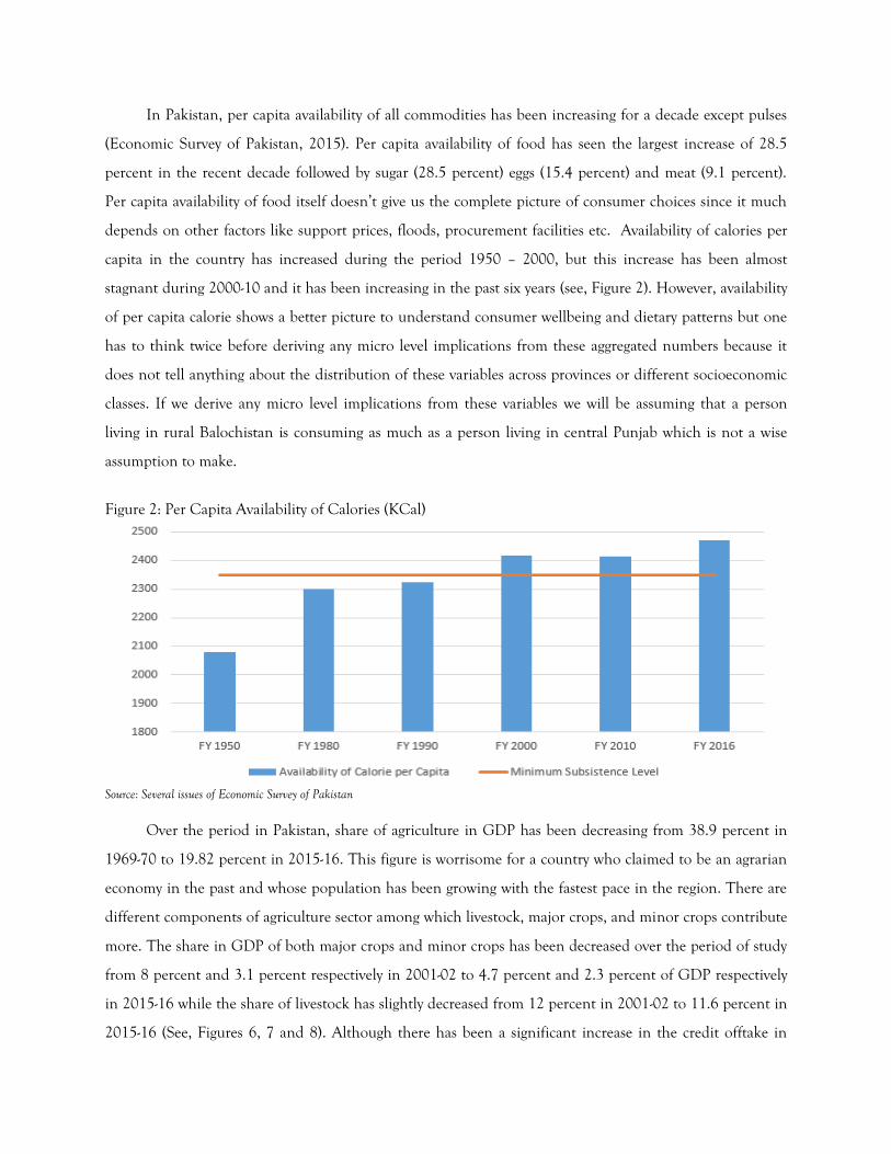
depends on other factors like support prices, floods, procurement facilities etc. Availability of calories per

capita in the country has increased during the period 1950 – 2000, but this increase has been almost

stagnant during 2000-10 and it has been increasing in the past six years (see, Figure 2). However, availability

of per capita calorie shows a better picture to understand consumer wellbeing and dietary patterns but one

has to think twice before deriving any micro level implications from these aggregated numbers because it

does not tell anything about the distribution of these variables across provinces or different socioeconomic

classes. If we derive any micro level implications from these variables we will be assuming that a person

living in rural Balochistan is consuming as much as a person living in central Punjab which is not a wise

assumption to make.

Figure 2: Per Capita Availability of Calories (KCal)

Source: Several issues of Economic Survey of Pakistan

Over the period in Pakistan, share of agriculture in GDP has been decreasing from 38.9 percent in

1969-70 to 19.82 percent in 2015-16. This figure is worrisome for a country who claimed to be an agrarian

economy in the past and whose population has been growing with the fastest pace in the region. There are

different components of agriculture sector among which livestock, major crops, and minor crops contribute

more. The share in GDP of both major crops and minor crops has been decreased over the period of study

from 8 percent and 3.1 percent respectively in 2001-02 to 4.7 percent and 2.3 percent of GDP respectively

in 2015-16 while the share of livestock has slightly decreased from 12 percent in 2001-02 to 11.6 percent in

2015-16 (See, Figures 6, 7 and 8). Although there has been a significant increase in the credit offtake in

agriculture sector (44.7 billion PKR to 385.54 billion PKR) along with the more distribution of improved

seeds (194000 tons to 455000 tons) and increased cropped area (22 million hectares to 23 million hectare)

but the water availability and the fertilizer offtake has remained almost stagnant during the period of study.

As far as the crop yields are concerned, there has been some increase in their yields. Yield (kg/hectare) of

wheat has increased by 22 percent, rice by 35 percent, sugarcane by 27 percent whereas maize has

experienced the exceptional growth of 143 percent from 2001-2016. However, the crop yields are increasing

over the period of time but there has not been much exceptional growth in yields since the green

revolution. Pakistan has low productivity in producing wheat and higher productivity in rice as compare to

the other regional countries.2 Productivity of wheat can be improved by using better seeds, farming

techniques and spreading awareness among farmers regarding the use of fertilizers, water, soil management

etc. Increasing only production is not enough as bottle necks in supply chain of wheat along with the price

distortions also needed to improve (See, Figures 9 to 15).

Livestock accounts for the biggest contribution to agriculture sector and there has been a quite

interesting trend in the livestock products where every single product has witnessed a handsome growth in

production except mutton. In case of mutton production, there has been a shift in trend, first increasing

production from 2001-2004 followed by a sharp decline in 2005-06 and then increasing again. First look at

the data suggest that this sharp decline in the production of mutton is due to the substitution effect as the

production of its close substitutes (beef and poultry meat) has experienced a sharp increase for the same

year but this notion requires detailed analysis (see, Figure 3). Beef production has seen a growth of 100

percent from 2001-2016 while it’s the poultry products which has seen the sharpest growth with the growth

of 245 percent in poultry meat and 116 percent in the production of eggs. Increasing by every year, milk

production in the country has observed a growth of 67 percent from 2001-2016.

However, numbers are showing an increased availability of food products but the improved

availability doesn’t ensure that everyone is getting the amount they required. Although the per capita

income has increased in last decade but increase in prices have been much more than the increase in per

capita income (See Appendix for the graphs). Prices of different products vary across provinces and cities

and also pretty much depends on the area in the same city from where you buy it. Some of these variations

are due to difference in quality but weaker price regulatory bodies are the prime reason for these

dissimilarities.

22 Yield (kg/hectare) of wheat in India = 3140; Bangladesh = 3013; Pakistan = 2752

Yield (kg/hectare) of rice in India = 2372; Bangladesh = 2299; Pakistan = 2479

To get the better estimates of prices, proxy for prices has been calculated from various issues of HIES

(See, Figures 17, 18 and 19). The reason for calculating a proxy instead of using the actual prices is that

HIES doesn’t collect data on prices and a better way to get prices from HIES is to calculate a proxy by

dividing quantities consumed of certain product by expenditure incurred on it. This will give us closer

estimates for what consumer has actually paid for the product in his/her environment. The sharpest rise in

the prices under the period of study is for FY2011. The main reason of this sharp increase in prices of

almost every food category is the international commodity price shock along with the oil price shock. In

2008, crude oil price reached its all-time high price of $145 per barrel which added in to the already

increasing commodity prices by increasing cost of transportation. Prices of cereals has witnessed the highest

increase during the period of study followed by the prices of meat, vegetables and dairy (See Appendix for

the graph). However, price differences are quite evident among provinces and even with in a province but

we are not going to discuss it in detail as price distortions is a separate topic of research and need much

attention.

Pakistan has witnessed regionally unbalanced economic growth since its beginning and this

unbalanced economic growth has significant contribution towards the current consumption patterns. Since

2001 to 2005 the country has seen an increase in the consumption inequality where rural regions observed

the highest increase in inequality with 6.4 percent increase in Gini coefficient followed by the urban region

with an increase of 5 percent (Anwar, 2009). The biggest cluster of people with high income per capita were

Figure 3: Three year Moving Average of Production of Meats (000 tons)

Source: Several issues of Economic Survey of Pakistan

estimated to be in the province of Punjab in 1998 as well as in 2005 (Ahmed, 2011). This tells us about that

the concentration of wealth at least geographically has remained the same since 1998.

To understand the consumption patterns and to make more robust implications out of analysis we

need to build our analysis on disaggregated level which would provide us with a better picture and would

highlight regional disparities, if there are any. Investigating ground realities always gives an edge to policy

makers to make more suitable and effective policies and make maximum use of their scarce resources. After

18th amendment, now more autonomous provinces can deal with the problems of food security, poverty

and malnutrition with more focus. However, the nature and quality of the transfers that have been made to

provinces is also an interesting topic of research. This study aims to highlight the problem of poverty and

regional disparities at national, interprovincial and intra-provincial level for Pakistan economy.

Furthermore, in the past, most of the analysis has been done on the aggregated level and there are few

studies done on the disaggregated level but most of them only focus on one province at a time (see

Table 1). The main research gap is that no significant study has been done at disaggregated level in

case of Pakistan so our main research motivation is to fill this research gap and contribute to empirical

literature at the disaggregated level which has some policy implication towards food security. The second

thing which motivated us to pick up this study is related to the use of superior technique of QUAIDS. Most

of the studies that have been done in context of Pakistan used linear Engel curves except (Iqbal & Anwar,

2014) which have applied QUAIDS but their work is at aggregated level (National and Provincial level) with

different food groups with independent price data and the importance of consumption bundles and

nutritional diversity is not included. However, this study will employ the technique of QUAIDS (Quadratic

Almost Ideal Demand System) at disaggregated level over different time horizons (from 2001 to 2014) to

capture temporal dynamics for horizontal and vertical comparisons. There are some growing concerns

related to micro-geographies of inequality in consumption pattern as well as in terms of food distribution

and this study will also contribute to literature in this direction.

One of the major reasons for choosing Pakistan as an empirical case for this study is because the

years under study (from 2001 to 2014) are the era of troubled times for Pakistan economy, due to war on

terror, financial and food price crisis occurred in 2007-08 and also democracy got better roots and stability

in Pakistan while on the other hand Pakistan experienced a devastating climate changes in terms of heat

waves and severe floods destroying agriculture crop production both food and cash crops as well as

improving vulnerability to poverty. Therefore, the present study tries to explore empirically three broad

areas of concerns: (a) to calculate the consumption bundles3 and investigate its differences over the period

3 Food expenditure shares

of study (at each cross section4), (b) to calculate expenditure and price elasticities and examine their

variability under different socioeconomic and demographic variables (i.e. consumption quintiles and

controlling for provinces and region), and (c) to calculate calorie intake and observe nutritional disparity in

inter and intra-provinces.

The rest of the paper is organized as follows: section two provides a comprehensive literature review,

section three discusses data and estimation methodology, results are elaborated in section four and five;

section six discusses policy implications; and finally last section concludes.

2. REVIEW OF LITERATURE The study of consumer behavior is dated back to 17th century when the first empirical demand schedule

was published (Davenant, 1700) referred by (Stigler, 1954). However, the study of how consumers allocate

their budget started from northern Europe dated back to 1840s but one of the most influential study in the

field till date was done by (Stigler, 1954) referred the work of (Engel, 1857) in which he postulated a law

which has set the foundation for future research work to come. In his study based on the data of

Ducpetiaux’s survey based on 153 Belgian families, the author identifies a pattern the way households

allocate their budget. He states that “a poor family allocate the greatest share of their expenditure to food

and as the family income increases this share becomes smaller”. This empirical observation was the first

generalization done on the base of survey data and it still plays an important role in modern

microeconomics, till dated. After this study, several other researchers (Laspeyres, 1875), (Farquhar, 1891),

(Benini, 1907) , (Persons, 1910), (Pigou, 1910), (Lenoir, 1913) and (Davies, 1975) done work on the same

topic with their different quantitative approaches and have significantly contributed in the field of

consumer behavior and budget allocations. In 1954 study, (Stigler, 1954) has done an impressive work in

which he described a brief history of the seminal work done by the other researchers. Since the scope of this

study is limited, it is important to mention only few studies which played an important role in refinement

of demand estimation techniques. Serious work done on the estimation of consumer behavior derived from

budgetary data started from earlier decades of 1900. In his study (Stigler, 1954) referred (Ogburn, 1919)

who used the budget data of Columbia district and calculated the expenditure share of each category

depending on following variables; family size and family income, which was incorporated using "equivalent

adult" scale.

For the data of Italian households (Stigler, 1954) referred the work of (Benini, 1907) who estimated

the demand for coffee and made the first application of multiple correlation to demand. There are number

4 2001-02, 2004-05, 2005-06, 2007-08, 2010-11, 2011-12, 2013-14

of studies after (Benini, 1907) which introduced several variables and techniques in attempt to incorporate

different aspects of consumer behavior5. The process of evolution is continuous and will take different

shapes with the improved data collection and estimation techniques that allow researchers in the future to

incorporate more variables of which data is not available yet.

The study of consumption patterns not only deal with the micro issues but it also has its significant

impact on the macro picture. In highly integrated economy a policy devised only for consumers will surely

end up having significant impact on other economic players of the system that is why it is important to

study how consumer in the economy is making its choices so one can make better micro or macro level

policies and also forecast for the future. In the 1960s Pakistan adopted a policy based on trickledown

economics whose underline agenda was to facilitate those who allocate greater portion of their income to

saving, so aim of this policy feature to lead us to higher amount of national saving which will then lead to

higher level of investment and improve the national income as a whole. Entrepreneurs are usually

considered to have higher level of marginal propensity to save than other economic players so on the bases

of primary household data of urban Karachi (Ranis, 1961) found that entrepreneurs have lower marginal

propensity to consume than the workers. Entrepreneurs have higher marginal propensity to save may be

because most of the entrepreneurs are in the higher income bracket which are more likely to save. Behavior

of the households are not likely to be same across whole country and sometimes there are huge regional

disparities with in a country. There are several other studies done on regional consumption disparities in

Pakistan (Rahman, 1963), (Hufbauer, 1968), (Khan M. I., 1969), (Khan & Khalid, 2011), (Khan & Khalid,

2012), (Malik, Nazli, & Whitney, 2014) and (Ahmad, Sheikh, & Saeed, 2015). Following table (Table 1) on

the next pages will give a brief overview of the work done on the topic in context of Pakistan. This study

aims to investigate different dimensions (i.e. primarily in context of consumption preferences, nutritional

disparity measured by daily calorie intake) of food consumption patterns some are already explored by the

authors mentioned above and some are still under-investigated. Differences among food consumption

patterns of rural and urban region and the differences among provinces are the points which are already

been investigated by researchers named below.

However, in our study, our empirical attempt is to find estimates at these levels as well as for the

differences with in a province with different food groups and by using a better technique (Quadratic AIDS).

In addition, this study will highlight the differences for intra-provincial disparities which will be its

contribution to the literature.

5 See for example, (Persons, 1910), (Pigou, 1910), (Lenoir, 1913) and (Davies, 1975)

If there are regional disparities among provinces, rural and urban areas then we cannot make a single

policy for all, as people in the different demographics would respond differently. According to a study

(Rahman, 1963) on average, cereal consumption in West Pakistan exceeds recommended intake levels by

nearly 23 percent. Probably only 10 percent of the West Pakistanis eat too little food grain from the

nutrition stand point. Overall, the diet is deficient in all foodstuffs except food grains. In terms of

Nutrients, household consumers from West Pakistan receives too little calcium, riboflavin, Vitamin A and

vitamin C (Hufbauer, 1968). There might be reasons other than the income levels for differences in

consumption patterns, sometime regional preferences play a significant role. Many researchers had done

work on the difference in consumption patterns of East and West Pakistan and one of the major factors

causing consumption disparity among these two units were the East Pakistan’s strong preference towards

rice and fish while West Pakistan’s preferences were towards cereals. In a study to understand food

consumption patterns (Khan M. I., 1969) author found out that a West Pakistani consumes more tonnage

of food than an East Pakistani but obtains less calories. The diet of urban consumers is more diversified

than their rural counterpart and urban consumers eat more of better quality food than rural consumers.

Better income distribution also plays a key role to uplift the living standards of those who are less privileged.

From the decade of 1970s Pakistan has seen a slight change in income distribution. This change in income

distribution was caused by different governmental policies6 and since the 1980s foreign remittances has

been playing an important role in our economy.

Table 1: Some Relevant Studies

Studies Year Brief findings A.A, Rahman 1963 Found results contradicting to Engle Law. Fresh fruits, poultry and meat

along with milk and milk products and vegetables are found to be luxury commodities where other as necessities.

G.C, Hufbauer 1968 On average, cereal consumption in West Pakistan exceeds recommended intake levels by nearly 23 percent. Overall, the diet is deficient in all foodstuffs except food grains. Expenditure elasticity of cereal is found to be 0.22 greater than its elasticity of physical consumption which is 0.15.

Mohammad Irshad Khan 1969 In West Pakistan, wheat is preferred cereal but not a preferred food; people have a tendency to shift to animal products for the major part of the calories if the income is permissive of such a shift.

Bussnik, C.F. Willem 1970 Results showed that the demand of other food grains and pulses will be positively affected by an increase in wheat price.

Rehana Siddiqui 1982 Based on HIES disaggregated data on rural and urban, study found the validity of the Engel's law for some commodity groups.

Aftab Ahmad Cheema; 1985 Results showed that the without much adverse effect on the households

6 These policies were based on the drastic shift of Pakistan’s economy from capitalism to socialism which includes land reforms

of 1972, job creation in public sector enterprises (PSEs) and migration of labor specially to Middle East which started inflows of

remittances in the country since late 1970s.

Muhammad Hussain Malik

with higher income per capita, consumption level of the poor households can be significantly increased.

Sohail J. Malik; Kalbe Abbas; Ejaz Ghani

1987 Estimated the coefficients and the slopes of consumption functions for urban and rural areas and fount them to be different for every year 1964-84. Therefore, he concluded that any effort of analysis using time series will give spurious results.

Harold Alderman 1988 Slope parameters differ across urban and rural regions, joint estimations, even when weighted, do not give accurate average responses.

Nadeem A. Burney; Ashfaque A. Khan

1991 Expenditure elasticities for commodity groups under study found to be variant with household’s income and generally shows a cyclic pattern. This cyclic behavior is explained by qualitative and quantitative changes in consumption basket. As we compare between households of rural and urban areas most of commodity groups differ in both structural and behavioral aspects which highlights the difference in consumption patterns of both areas.

Sohail J. Malik; Nadeem Sarwar

1993 Consumption patterns are different among rural urban regions as well as among all provinces. In Pakistan, marginal propensity to spend is lower for the households receiving international remittances.

Sonio R Bhalotra, Cliff Attfield

1998 Authors didn’t find any evidence in the favor of biasness among children of different sex and different birth order and there is also not significant evidence in favor of the notion that elderly get different treatment. Results also showed that adult goods, food and child goods have non-linear Engel curves.

Eatzaz Ahmad; Muhammad Arshad

2007 Results showed that the households living in rural areas consider following items as absolute necessities housing, tobacco, wheat, clothing and foot wear while among middle-income class wheat is considered to be an inferior good. In case of urban households housing, health, wheat is found to be absolute necessities.

Ashfaque H. Khan; Umer Khalid

2011 Consumption patterns are found to be different among rural urban regions as well as among provinces. Results showed that the household consumers spend the greatest proportion on food and drinks.

Ashfaque H. Khan; Umer Khalid

2012 Findings showed that a greater share of financial resources has been devoted to education and health care by Female Headed Households as compare to their main counterparts.

Sohail Jehangir Malik; Hina Nazli; Edward Whitney

2014 Results found limited dietary diversity amongst Pakistani households. Average household consumes less than the recommended number of calories (2350 KCal). Rural and urban areas are found to have different consumption patterns.

Zahid Iqbal; Sofia Anwar 2014 Result confirms the differences in food consumption levels along with the differences in expenditure and price elasticities.

Nisar Ahmad; Muhammad Ramzan Sheikh; Kashif Saeed

2015 Consumption patterns between urban and rural households are found to be different and households with higher income tend to spend more on milk, fish, meat and rice as compare to their counterparts which tend to spend more on pulses, vegetables and wheat.

Pakistan’s current account balance has always been dependent on remittances and these remittances

also play a crucial role in uplifting the social status of the recipient households. There is a debate in

literature about the use of remittances while some people consider it to be used only for nonproductive

purposes by households, other consider it to be one of the most important factor for increasing the

socioeconomic status of the household. Remittances has also been found a significant factor in determining

consumption patterns for Pakistan households (Malik & Sarwar, 1993). Urban households who receive

remittance are likely to consume greater share of their income than their rural counterpart and at country

level the households which are receiving international remittances are tend to devote lesser share of their

income to expenditure than those who are receiving domestic remittances. The marginal propensities are

highest for the domestic migrant households followed by non-migrant households and international

migrant households having marginal propensities to spend 0.64, 0.52 and 0.57 respectively. Marginal

propensities to spend on total expenditures are lowest in rural KPK and highest in urban Punjab. Marginal

propensities to spend for households who does not receive remittances are lowest for urban Sindh and

highest for rural Sindh.

It has been observed that more equitable distribution will stimulate demand for basic necessities as

the people who are in the bottom income quintile are mostly deprived of most of necessities (Cheema &

Malik, 1985). The impact of an increase in income has also significant impact on consumption expenditure,

(Ali, 1985) in his analysis of household consumption and saving behavior assessed that an increase of 10

percent in the income per person would increases the household’s total expenditure by 7.3 percent and out

of a rupee increase in consumption expenditure, 28 percent goes to food. As per capita income of

household rises, it effects household in several aspects and the demand for different products changes as

per their nature which is determined by their elasticities. Results of earlier work done by many researchers

confirms the validation of Engel law7 however the underlined functional form has remained debatable over

the period of time. The estimated values of elasticities are highly related with the functional form that has

been used to calculate them, so as we change the underline functional form it will give different estimated

values. The difference between these estimated values depends on the nature of the data set as well as the

severity of the change in functional form.

Expenditure elasticities for various commodity groups differ with the different socioeconomic

variables8 (Burney & Khan, 1991) showed it in a repeated manner, which is described in the form of

qualitative and quantitative alterations in the household’s consumption bundle. It is difficult to absorb

difference in the quality of products consumed by different tiers of households. Although, there are

yardsticks to measure quality but variables measuring quality are not provided in HIES and PSLM. 7 Engel law states that with an increase in income there will be decrease in share of income spent on food even if

absolute expenditure on food increases. 8 They calculated consumption elasticities for different income groups and also used additive and multiplicative

dummy variables to highlight the difference among income groups.

However, difference in prices among different provinces gives us a rough estimate but this idea becomes

vague if we bring in the concept of comparative advantage, transportation cost and access to road from

households.

It has also been noticed (Khan & Khalid, 2012) that household with the same resources tends to

choose different consumption bundles based on the gender and the education level of the household head.

It is important to narrow our focus to specific household characteristics which would give us acute policy

implications9. In their study to evaluate the differences in income allocation between households headed by

male and female (Khan & Khalid, 2012) concluded that the households who are headed by females allocate

greater share of their resources to productive avenues like increasing education level or getting training to

enhance their skills.

Commodity prices are at their low these days which is estimated to change the way consumer

optimize their consumption bundle due to the fact that lower level of prices would increase purchasing

power of consumers. The current scenario is totally opposite of the situation which occurred from mid to

late 2000s due to commodity price shock, which had drastically reduced the consumer’s purchasing power.

So it is also important to see that how consumers change their consumption bundles in response to change

in their real purchasing power. As price of commodities changes, consumer’s real purchasing power also

changes; for example: if price increases by 100 percent then the consumer will only able to buy half of the

products that he was able to buy before change in prices. Consumers are expected to adapt the situation to

make changes in their consumption bundle in response to price change. The effect of prices on consumer’s

quantity demanded of a certain good can be disintegrated into substitution effect and income effect.

Income effect captures the changes in consumption choices in response to change in consumer’s real

income where substation effect shows the effect of price changes on consumption bundle keeping

consumer’s real income constant.

Food prices has found to be the most important factor in determining the level of demand for other

commodities, total expenditure and saving (Ali, 1985). In Pakistan, people who are unable to make it even

half of the poverty line10 are high as 2.3 million while the number of people who are just below the poverty

line are 13.7 million and there are 10 million more than that who are just above the poverty line (Haq,

Nazli, & Meilke, 2008). As now government of Pakistan has changed its methodology to calculate poverty

line by abandoning the Food Energy Intake (FEI) method and adopting new method of Cost of Basic Needs

9 If we can boil down our model to specify the cluster of households by specific characteristics like gender of the head, education

of the head, number of children, etc. So we can make targeted policy implications which will not only save our time and

resources but will also be more effective than other options. 10 Previously poverty line in Pakistan was calculated by cost of minimum required calorie intake of 2350 calories per adult equivalent per day.

(CBN) for capturing non-food expenditures the percentage of population living under poverty has now

jumped to 30 percent. Food consumption has significance especially in a country where average consumer

spends almost half of his income on food. The problem of getting lower calorie intake is not solely based on

the low income levels, quality and availability of food but it also depends on the choice of consumption

bundles whether the consumer is having a balanced diet or not. When there is lack of awareness,

consumers often end up having unbalanced diet which effects their health status in the long run. The scope

of this paper is limited so I would like to bring the focus back to calorie intake and consumption bundle. A

consumer would be in a better position to get a balanced diet if he is fully aware or at least have some

knowledge about the calorie content of the products he is using. In this way a consumer can optimize his

diet given his financial constraints.

Sometimes price response may tend to vary among different market, cities and other demographic

variables e.g. Bigger cities have better organized markets that encourage competition and will lead to more

variety and lower price level compare to small isolated markets. In case of Spain, consumers’ responsiveness

to price were greater in large central cities in comparison to rural areas (Navamuel, Morollón, & Paredes,

2014). The main reason of prices being lower in the large central cities is competitive markets and high

population density which allow retailers to operate at lower margins and make profits on the basis of

volume of their sales. Results like these implies that we need to be specific in our policy making because

consumer living in big cities may respond to the same policies differently than the people living in rural or

urban areas with small markets.

Urbanization and trade openness also plays a vital role in altering the consumption patterns.

Increased trade gives consumer more variety to choose from so they are likely to alter their consumption

bundles (Hovhannisyan & Gould, 2011) (Kearney, 2010). It has also been estimated that people across the

globe on average allocate the highest share of their income on food (25%) (Selvanathan & Selvanathan,

2006). China is one of the fastest growing economy in the world and this growth has increased the real

purchasing power of Chinese consumers which has altered their dietary patterns. Dietary patterns of an

average household have now incorporated elements like fine grains into their traditional diets

(Hovhannisyan & Gould, 2011). This change might be caused due to the fact that trade liberalization has

provided greater variety to Chinese consumers which were not available before. The change in consumption

patterns might not be similar across different regions and different socioeconomic classes. India has also

witnessed a change in consumption pattern and this change was found to be significant for both rural and

urban regions (Viswanathan, 2001). Indian household consumers of lowest quintiles were found to allocate

more of their income to non-food expenditures then they were allocating before which has caused by the

price changes in rural areas and income changes in urban areas. For the households in middle and upper

quintiles this change has not only been limited to a shift from food to non-food products but also have

increased the diversity of food basket by including more fruits and vegetables.

It has been seen that consumers in urban areas are tends to have more diversified consumption

bundle than their rural counterpart. Diversified consumption bundle allows people to have better

nutritional status than those whose dietary patterns are composed of only few products. In Pakistan, there is

limited dietary diversity among Pakistani households (Malik, Nazli, & Whitney, 2014). Large number of

population consumes less than the required number of calories and these trends are heterogeneous among

rural and urban regions and also vary among different socioeconomic classes. In this study I aim to discover

disparity in average household’s consumption patterns, calorie intake and their responsiveness to changes

in price and income. We will be calculating and highlighting these disparities in different regions (rural and

urban), among provinces and within a province for a period of 2001-2014. To the best of our knowledge

there has been no comprehensive study done to investigate consumption pattern disparity among all these

tiers (National, Inter-Provincial and Intra-Provincial) and we expect consumption patterns to be

heterogeneous at these levels on the basis of the fact that Pakistan as a country have seen regionally

unbalanced growth since the beginning. Varying levels of income, education, market structure, law and

order situation and there are many other factors which have caused these differences at different levels over

the period of time but the scope of this study is to only highlight the differences and their severity.

3. DATA AND EMPIRICAL METHODOLOGY 3.1 Data In this study, the analysis done on six latest data sets (2001-02, 2005-06, 2007-08, 2010-11, 2011-12 and

2013-14) of Household Income Expenditure Survey (HIES) which covers the period from 2001-2014.

Pakistan Bureau of Statistics (PBS) conducts HIES since 1963 later it was merged with the Pakistan

Integrated Household Survey (PIHS). The latest available dataset is of HIES 2015-16 which is not included

in this study. The primary reason is that, the coding scheme for various commodity groups in HIES 2015-16

has been revised and updated. We plan to consider this survey round in our future research work. For

current study, average household size and sample size for HIES datasets (2001-02, 2005-06, 2007-08, 2010-

11, 2011-12 and 2013-14) are given below.

Summary Table Year Sample Size of Households Average Family Size

Rural Urban Total 2001-02 10233 5949 16182 7.21 2004-05 8899 5809 14708 6.69 2005-06 9213 6240 15453 7.17 2007-08 9257 6255 15512 6.9 2010-11 9752 6589 16341 6.66 2011-12 10481 6743 17224 6.73 2013-14 11755 6234 17989 6.61

Note: Authors’ computations from HIES datasets. 3.2 Empirical Methodology Calculating elasticities, for different demographic variables and socioeconomic classes, is one of the

objectives of this study to fulfill for which we need to choose an appropriate econometric model along with

a suitable statistical technique. There are several techniques which can be used to complete this task but

every technique has its own advantages and disadvantages. Therefore, to make results stable and robust the

selection of best available technique is of dire importance.

(Rahman, 1963), (Siddiqui, 1982) (Burney & Khan, 1991), (Khan & Khalid, 2011) (Khan & Khalid,

2012) employed the technique of Linear and Double Logarithm Engel Curves where, (Bussnik, 1970) used

Augmented Engel Curve, (Ali, 1985) worked with Extended Linear Expenditure System, (Malik, Abbas, &

Ghani, 1987) used the functional form of Generalized Least Square (GLS) and (Malik & Sarwar, 1993)

preferred OLS for estimation and more recently (Ahmad et al., 2015) did his study with Linear Engel

Curves. There are few authors who have tried to use many techniques to check differences in their

estimated results like (Cheema & Malik, 1985) did using several techniques. However, availability of so

many techniques makes you comfortable but such a wide range of options sometimes confuse your which

technique to use. That is one of the important reason why some authors try to come up with new

techniques which can suit better with the properties of data and the nature of the analysis.

(Farooq, Young, & Iqbal , 1999), (Viswanathan, 2001), (Haq, Nazli, & Meilke, 2008), (Bertail &

Caillavet, 2008), (Malik, Nazli, & Whitney, 2014), (Navamuel, Morollón, & Paredes, 2014) used the linear

specification of AIDS developed by (Deaton & Muellbauer, 1980). This technique is considered to give

more flexibility in demand curve estimation and fulfills more properties of the demand curve. AIDS derives

budget share equation using the cost function introduced by (Muellbauer, 1976) named PIGLOG cost

functions. However, (Bhalotra & Attfield, 1998) investigated that semi parametric estimates of Engel curves

for rural Pakistan suggest that the popularly used (PIGLOG) class of demand models is in appropriate. The

data favor a quadratic logarithm specification. In the case of food, the results for Pakistan stands in contrast

to that for the US, UK and Spain, all of which have Engel curves linear in the logarithm of expenditure. To

address the issue of dynamics of the Engel curves (Ahmad & Arshad, 2007) used Spline Quadratic Engel

Equation System which can incorporate bulges of the Engel Curves. This study finds that the resulting

flexibility produces many interesting patterns of changes in the classification of goods into necessities and

luxuries across income ranges. These patterns can be taken into account for various tax policy experiments

for better design of welfare policies in Pakistan.

For other empirical studies, table (Table 2) tries to summarize the techniques being used in similar

topics in context of different countries, including Pakistan.

Table 2: Techniques used by other Researchers

Authors Years Techniques Used

Gustav Ranis 1961 Parabolic Consumption Functions

A.N.M. Azizur Rahman 1963 linear and double log form

G.C. Hufbauer 1968 Linear Engle Curve

Muhammad Irshad Khan 1969 Linear Engle Curve

Willem C.F. Bussnik 1970 Augmented Engel Curves

Aftab Ahmad Cheema; Muhammad Hussain Malik

1985 Linear, log-log, semi-log, ratio of semi log inverse and log - log inverse.

M. Shaukat Ali 1985 Extended Linear Expenditure System

Sohail J. Malik; Kalbe Abbas; Ejaz Ghani 1987 GLS and different tests to check pooling

Harold Alderman 1988 Linear Almost Ideal Demand System (LAIDS)

Nadeem A. Burney; Ashfaque H. Khan 1991 linear and double logarithm Engel Curves

Sohail J. Malik; Nadeem Sarwar 1993 OLS

Sinio R Bhalotra; Cliff Attfield 1998 Several estimation techniques

Umar Farooq; Trevor Young; Muhammad Iqbal

1999 Linear Almost Ideal Demand System (LAIDS)

Brinda Vishwanathan 2001 Linear Almost Ideal Demand System (LAIDS)

Eliyathahby Antony Salvanathan; Saroja Salvanathan

2003 Rotterdam Model

Eliaz Mantzouneas; George Mergos; Chrysostomos Stoforos

2004 ECM formulation of AIDS

Eatzaz Ahmad; Muhammad Arshad 2007 Spline Quadratic Engel Equation System

S. Limba Goud 2010 Double Log Expenditure Function

Vardges Hovhannisyan; Brian W. Gould 2011 Generalized Quadratic AIDS

Ashfaque H. Khan; Umer Khalid 2011 linear and double logarithm Engel Curves

Ashfaque H. Khan; Umer Khalid 2012 linear and double logarithm Engel Curves

Elena Lasarte Navamuel; Fernando Rubiera Morollon and Dusan Paredes

2014 Linear Almost Ideal Demand System (LAIDS)

Sohail Jehangir Malik; Hina Nazli; Edward Whitney

2014 Linear Almost Ideal Demand System (LAIDS)

Zahid Iqbal; Sofia Anwar 2014 Quadratic Almost Ideal Demand System (QUAIDS)

Nisar Ahmad; Muhammad Ramzan Sheikh; Kashif Saeed

2015 Linear Engle Curve

Motivating from earlier attempts, if we incorporate the approach of (Bhalotra & Attfield, 1998) then

we are left with fewer choices after eliminating linear models. For this analysis the quadratic specification of

AIDS has been used. As of today, this technique has not been so commonly used for analysis of the

household datasets in Pakistan, except (Iqbal & Anwar, 2014). In order to use this technique, following

variables are required: income, prices, quantity demanded, and food bundle shares in total expenditure on

food. In household surveys of Pakistan, the data on income is not much reliable as people tend to

underreport their income therefore to tackle this problem (Houthakker, 1970) recommended to use total

spending as an alternative of permanent income. The use of total expenditure as permanent income may

often lead to the problem of economies of scale. Households’ total expenditure can be bifurcated into these

two effects which are ‘income effect’ and ‘specific effect’.

The specific effect captures the increase in necessities demanded because of increase in household

size where the income effect refers to the effect of increase in household size at given level of income which

decreases per capita income of household and makes everyone poorer. To tackle this problem, we used the

variable of expenditure per capita which can be calculated by dividing total household expenditure and by

household size (both can be calculated using HIES dataset). Another problem which arises using HIES

datasets is that it does not collect data for prices of commodities consumed. However, data of expenditure

done on the specific products and their quantity consumed are available in the datasets which can be used

to find a close proxy for prices of the products. Underline estimation method used in this study to estimate

QAIDS is non-linear seemingly unrelated regression. This method is the extension of LA-AIDS as

developed by Deaton and Muellbauer (1980a,b).11 The nonlinear extension of LA-AIDS has been done by

Banks, et al., (1997).12

In this study household consumer’s demand for following eleven food groups is considered: wheat,

rice, other cereals, pulses, fresh fruits, vegetables, dairy, meats, oils, sugars and others (tea, coffee, spices and

condiments etc.). Model used in the estimation is based on the following indirect utility function:

11 Deaton, A., and J. Muellbauer (1980a). "An Almost Ideal Demand System", American Economic Review, 70 (3): 12-26 Deaton, A., and J. Muellbauer (1980b). Economic and Consumer Behavior, Cambridge University Press 12 Banks J, Blundell R, Lewbel A. (1997): Quadratic Engel Curves and Consumer Demand. The Review of Economics and Statistics, 79(4): 527–539.

ln 𝑎(𝑝) = ∝0+ ∑ ∝𝑖 ln 𝑝𝑖

𝑘

𝑖=1

+1

2 ∑ ∑ 𝛾𝑖𝑗 𝑙𝑛𝑝𝑖 ln 𝑝𝑘

𝑘

𝑗=1

𝑘

𝑖=1

(1)

Where; in the above transcendental logarithm function subscript 𝑖 denotes the category of food group

therefore, pi is the price of the ith food group. Following is the equation of Cobb-Douglas price aggregator:

𝑏 (𝑝) = ∏ 𝑃𝑖𝛽𝑖

𝑘

𝑖=1

𝜆(𝑝) = ∑ 𝜆𝑖

𝑘

𝑖=1

ln 𝑝𝑖

In the equation above ∝0 could be estimated jointly with other parameters but in practice as most of the

researchers set its value slightly less than the lowest value of the logarithm of total expenditures which can

be easily calculated from the data. Adding up, homogeneity13 and slutsky symmetry14 requires the following

restrictions to be imposed:

∑ ∝𝑖= 1, ∑ 𝛽𝑖 = 0

𝑘

𝑖=1

𝑘

𝑖=1

, ∑ 𝛾𝑖𝑗 = 0

𝑘

𝑗=1

, ∑ 𝜆𝑖 = 0

𝑘

𝑖=1

𝑎𝑛𝑑 𝛾𝑖𝑗 = 𝛾𝑗𝑖

By applying Roy’s identity to equation (1) which is the equation of indirect utility, I obtain the

expenditure share equation:

𝑤𝑖 = ∝𝑖+ ∑ 𝛾𝑖𝑗

𝑘

𝑗=1

𝑙𝑛𝑝𝑗 + 𝛽𝑖 𝑙𝑛 {𝑡𝑜𝑡𝑎𝑙 𝑒𝑥𝑝𝑒𝑛𝑑𝑖𝑡𝑢𝑟𝑒

𝑎(𝑝)} +

𝜆𝑖

𝑏(𝑝) [ln {

𝑡𝑜𝑡𝑎𝑙 𝑒𝑥𝑝𝑒𝑛𝑑𝑖𝑡𝑢𝑟𝑒

𝑎(𝑝)}]

2

(2)

𝑖1→𝑘 𝑎𝑛𝑑 𝑗1→𝑘

Here 𝜆𝑖 is the coefficient of quadratic term. If 𝜆𝑖 becomes zero in any case, then the model above

will be reduced to linear version of AIDS.

Demographic variables are also incorporated in this study by using scaling technique introduced by

Ray (1983) and developed by Poi (2002a and 2012) to the quadratic specification of AIDS. Here we use a

vector m which represents s characteristics. This matrix can incorporate number of characteristics and the

simplest can represent only one characteristic which will make m a scalar quantity. Let

𝑒𝑥𝑝𝑒𝑛𝑑𝑖𝑡𝑢𝑟𝑒𝑍(𝑝𝑟𝑖𝑐𝑒, 𝑢𝑡𝑖𝑙𝑖𝑡𝑦) be a representative function of a randomly chosen household so this

household might only be consisting of only one member. Ray suggested Ray to use following expenditure

function for each household: 13 The effect of increase in prices is proportional to increase in expenditure on food. 14 Cross partial effects are always equal.

𝑒𝑥𝑝𝑒𝑠𝑛𝑑𝑖𝑡𝑢𝑟𝑒 (𝑝𝑟𝑖𝑐𝑒, 𝑚, 𝑢𝑡𝑖𝑙𝑖𝑡𝑦) = ℎ0(𝑝𝑟𝑖𝑐𝑒, 𝑚, 𝑢𝑡𝑖𝑙𝑖𝑡𝑦) × 𝑒𝑥𝑝𝑒𝑛𝑑𝑖𝑡𝑢𝑟𝑒𝑍(𝑝𝑟𝑖𝑐𝑒, 𝑢𝑡𝑖𝑙𝑖𝑡𝑦)

To scale the expenditure function Ray used the function ℎ0(𝑝𝑟𝑖𝑐𝑒, 𝑚, 𝑢𝑡𝑖𝑙𝑖𝑡𝑦) to incorporate

household attributes. This function can be further decomposed as:

ℎ0(𝑝𝑟𝑖𝑐𝑒, 𝑚, 𝑢𝑡𝑖𝑙𝑖𝑡𝑦) = ℎ̅0(𝑚) × 𝜃 (𝑝𝑟𝑖𝑐𝑒, 𝑚, 𝑢𝑡𝑖𝑙𝑖𝑡𝑦)

Both terms used in the above function are placed to absorb different effects. The first expression

ℎ0(𝑚) processes the effect of increase in household’s expenditures subject to the matrix m which is

incorporating different household characteristics without incorporating the changes in consumption

bundle or price effects; a household composed of t members will spend more than the household

composed of k members if 𝑡 > 𝑘. The second expression in the above term controls for changes in actual

goods consumed and relative prices; a household with two infants five children and four adults will

consume quite differently from the one composed of five adults. As suggested by Ray (1983), ℎ̅0(m)

parameterized as:

ℎ̅0(𝑚) = 1 + 𝜏′(𝑚)

here 𝜏 is a vector of parameters to be estimated. 𝜃(𝑝𝑟𝑖𝑐𝑒, 𝑚, 𝑢𝑡𝑖𝑙𝑖𝑡𝑦) is parameterized as:

𝑙𝑛𝜃(𝑝𝑟𝑖𝑐𝑒, 𝑚, 𝑢𝑡𝑖𝑙𝑖𝑡𝑦) =∑ 𝑃

𝑗

𝜎𝑗(∏ 𝑃𝑗

𝛿′𝑗𝑚

− 1)𝑘𝑗=1

𝑘𝑗=1

1𝑢𝑡𝑖𝑙𝑖𝑡𝑦

− ∑ 𝜆𝑗 𝑙𝑛𝑃𝑗𝑑𝑗=1

This functional form has an edge over other forms that it results in expenditure share equations

that closely follows other equations which do not incorporate demographics. Here 𝛿𝑗 represents the jth

column of 𝑘 × 𝑑 parameter matrix 𝛿. Following is the equation of expenditure shares.

𝑤𝑖 = ∝𝑖 + ∑ 𝛾𝑖𝑗 ln 𝑃𝑗

𝑘

𝑗=1

+ (𝛽𝑖 + 𝛿𝑖′𝑚) ln {

ℎ

ℎ̅0(𝑚)𝑎(𝑃)} +

𝜆𝑖

𝑏(𝑝)𝑐(𝑃, 𝑧) [𝑙𝑛 {

ℎ

ℎ̅0(𝑚)𝑎(𝑃)}]

2

(3)

𝑖1→𝑘 𝑎𝑛𝑑 𝑗1→𝑘

Where, 𝑐(𝑃, 𝑚) = ∏ 𝑃𝑗

𝛿𝑗′𝑚𝑘

𝑗=1

In order to satisfy the adding up property ∑ 𝛿𝑖𝑗𝑘𝑗=1 = 0 for r=1s. In this study I’ll be calculating the

compensated price elasticities, uncompensated price elasticities and expenditure elasticities. Following is the

formula for uncompensated price elasticity of good 𝑖 with respect to change in price good 𝑗:

𝜖𝑖𝑗 = −𝜋𝑖𝑗 +1

𝑤𝑖𝑗 (𝛾𝑖𝑗 − [𝛽𝑖𝑗 + 𝛿𝑖

′𝑚 +2𝜆𝑖

𝑏(𝑃)𝑐(𝑃, 𝑚) 𝑙𝑛 {

ℎ

ℎ̅0(𝑚)𝑎(𝑃)}] × (∝𝑗+ ∑ 𝛾𝑗𝑙 ln 𝑃𝑙

𝑙

)

−(𝛽𝑗 + 𝛿𝑗

′𝑚)𝜆𝑖

𝑏(𝑃)𝑐(𝑃, 𝑚)[𝑙𝑛 {

ℎ

ℎ̅0(𝑚)𝑎(𝑃)}]

2

)

𝑖1→𝑘 𝑎𝑛𝑑 𝑗1→𝑘

(4)

The expenditure (income) elasticity of good i can be obtained from the following formula:

𝜇𝑖 = 1 +1

𝑤𝑖 [𝛽𝑖 + 𝛿𝑖

′𝑚 + 2𝜆𝑖

𝑏(𝑃)𝑐(𝑃, 𝑚) 𝑙𝑛 {

ℎ

ℎ̅0(𝑚)𝑎(𝑃)}] (5)

Slutsky equation (𝜖𝑖𝑗𝑐 = 𝜖𝑖𝑗 + 𝜇𝑖𝑤𝑗) can be used to find compensated price elasticities.

Here I’ll use the estimation technique of iterated feasible generalized nonlinear least-squares to estimate

the parameters.

4. FOOD CONSUMPTION PATTERNS In this section we will be discussing the trends and changes in food consumption bundles, calorie bundles

and cost of calories. This section will do the multi-tier analysis as the variables are calculated at national

level, provincial level and as well as sub-provincial level. By sub-provincial level we mean the difference

between urban and rural regions of a particular province which will enable us to highlight the rural urban

diversity in the provinces. See the chart below to have a better look to understand different tiers of analysis.

4.1 Food Consumption Bundles The share of food expenditure in the total expenditure has been more than 50 percent during 2001-2016

except for the year 2004-05 where it fell down to 48 percent. On average, the food expenditure shares in

total expenditure for 2001-2016 has remained 51 percent. This share has been relatively as low as 45

percent for the urban areas while for rural areas this share jumps to 55 percent having its highest value of

59 percent in 2010-11. This share increases as we move towards the families having lower per capita income

and decreases as shift our focus to the families having higher per capita income (See, Figure 4). If we look at

these shares at the provincial and sub provincial levels, then urban Punjab has the lowest share (42 percent)

of food expenditure in total expenditure followed by urban Sindh (43 percent) while the largest shares are

found to be in rural Balochistan (55 percent) followed by rural KPK and rural Sindh both at 54 percent (see

Figures 20 and 21). These shares tell us pretty much about the income level in these regions as according to

Engel law “share of food expenditures in total expenditures tend to decrease with an increase in total

income” and our food expenditure shares are in line with the reality as central Punjab is economically the

most prosperous region followed by the urban Sindh (Ahmed, 2011).

On the aggregate level, the biggest share of this food expenditure is accounted for dairy products

which was 27 percent of the total food expenditure in the year 2013-14. The second biggest share of the

food expenditure is accounted for Wheat (16 percent) followed by Meats (12 percent) and Vegetables (10

percent) in the year 2013-14. The share of wheat is greater for rural region as compared to urban region

whereas shares of dairy and meats are greater for urban region while share of vegetables remains same in

both regions. Share of wheat has been almost stagnant for urban regions while its share has been increasing

for rural regions during the period of study. However, the shares of different food categories are different

at aggregate, urban and rural level but the ranking of the top four food groups are the same where dairy

being at top of the list followed by wheat, meat and vegetables. This ranking remains the same with

different values for expenditure shares for all provinces except for Balochistan in which wheat has the

highest average expenditure share of 20 percent followed by meats (17 percent), dairy (14 percent) and

vegetables having average share of 11 percent (See Figures 22 to 38).

0

20

40

60

80

100

2001-02 2004-05 2005-06 2007-08 2010-11 2011-12 2013-14Wheat Rice Other CerealsPulses Fruits VegetablesDairy Meats OilsSugars Other Food share in Total Exp.

Figure 4: Consumption Bundles at National Level

Source: Author’s calculations from several issues of HIES

If we divide these numbers by bottom and top income quintiles, then we can highlight the

differences between consumption bundles of both income groups. Households which lies in the bottom

income quintile spends more on wheat as their average food expenditure share on wheat is 24 percent for

the period under study. The first rank of wheat is followed by dairy (18 percent), Oils & fats (12 percent)

and vegetables (11 percent). This consumption bundle contrasts with the consumption bundle of the

households in top quintile which spends most on dairy products (26 percent) followed by meats (15

percent), other products (13 percent) and finally wheat (11 percent). Wheat is the most important food

group in bottom quintile of all provinces having its largest share of 27 percent for Balochistan followed by

26 percent in KPK, 25 percent in Punjab and 21 percent in Sindh. Dairy products have the second largest

share in all provinces except Balochistan in which vegetables and meats have a similar average share but

share of vegetables has been increasing during the period of study while the share of meats is at a decreasing

trend. Oils and fats has the third largest share in all provinces where in Sindh food group of vegetables also

shares the same position (see Figures 22 to 38).

In contrast with the bottom quintile, the people in top income quintile spends the biggest share of

their food expenditure on dairy products in all provinces except Balochistan in which the largest share is

possessed by meats. Meats has the second biggest food share in Sindh and Punjab, in KPK the second rank

is shared by meats and wheat while dairy products are at the same position in Balochistan. The food shares

of meats and dairy products have an increasing trend while the share of wheat has been declining over the

period of time. Other interesting thing which can be seen by the food shares of top income quintile is that

food group of other products has the third biggest food share in Sindh and Punjab. The analysis using

income quintiles clearly contrasts the consumption pattern of both groups where poor spending more on

the basic necessities like wheat and rich spending more on dairy and meats.

4.2 Calorie Bundles It is important to understand the importance of calorie bundles because the diet we consume today is the

most important determinant of our health in the future. Wheat is the most important product in the

calorie bundle of the country as its average share in calorie bundle is 48 percent. This share soars up to 50

percent in case of rural households and shrinks to 44 percent in case of urban consumers. However, its

share has been declining over the period of time but it is still the most important ingredient in the calorie

bundle of the country. The second biggest share in the calorie bundle is occupied by the fats & oils having

average calorie share of 14 percent and the alarming thing is that this share is increasing over the period of

time. For urban households the third most important food group by calorie share is dairy products15 (11

percent) followed by sugars (10 percent). In contrast to urban households, sugars have the third largest

share in calorie bundle (11 percent) followed by dairy products (10 percent).

Not surprisingly wheat has the biggest share in calorie bundle of each province having its highest

share of 54 percent for rural Balochistan and its lowest share of 38 percent for urban Sindh. Oils & fats

have the second biggest share in the calorie bundle for all provinces but in the case of Punjab, dairy

products also have the same average share in calorie bundle. Dairy products have the third largest share in

calorie bundles of all provinces except for Punjab in which this position is taken by sugars. For urban

regions dairy products have the third biggest share in calorie bundles of Sindh and Punjab after wheat and

oils & fats. In contrast to Sindh and Punjab, sugars have the third largest share in calorie bundles of KPK

and Balochistan. For rural Punjab, dairy products have the second biggest share in calorie bundle followed

by fats and oils. Unlike rural Punjab, in rural Sindh second largest share has been occupied by fats and oils

followed by the sugars. In contrast to bundles in other provinces rural KPK and rural Balochistan has both

sugars along with fats and oils at the second position followed by dairy products (see Figures 39 to 46).

To have a balanced diet our food should mainly composed of grains and cereals followed by fruits

and vegetables. All kind of meats along with dairy products comes after fruits and vegetables and fats & oils

with sugars have the smallest shares. So far all the estimated consumption bundles are missing this dietary

diversity which is the main reason of malnutrition among masses. The other most important thing which is

absent in these dietary patterns is the use of vegetables and fruits and this is the surprising thing for the

country who claims to be an agrarian economy. Pakistani households need to diversify their diet to fight

malnutrition and possible health risks.

4.3 Cost of Calories The data shows that the diet of Pakistani households have not been efficient in terms of expenditures. After

having the per AE expenditure and calorie contribution of each food group we calculated the cost of 100

kilo calories. The cost of calories is quite reliable estimate to get an idea what consumer is actually paying

for each calorie consumed from different food groups and by how much cost of calories from these groups

differ. The cheapest source of calories at all levels is not surprisingly wheat this is one of the most important

reasons why we see wheat having the largest share in calorie bundle. The second cheapest source of calories

is sugars followed by fats & oils and rice. The cost of calories for almost every food group is higher in urban

15 If we also include desi ghee in dairy products instead of fats & oils, then the share of dairy products will increase both in food

expenditure and calorie bundle.

areas as compare to the rural areas. One possible reason for the cost of calories being lower in rural areas

could be the fact of rural region being net producer of food products.

Meats has found to be most expensive source of calories followed by the fruits and vegetables. Five

out of eleven food groups have seen rise in the cost of calories during 2001-2014 (see, Table 3 and Figures

47 to 53). Similar patterns have been observed in the case of other food groups. The cost incurred in

gaining calories from wheat has been lowest in rural Punjab which is aligned with the fact that the region is

the largest producer of wheat in the country. The cost attributable to vegetables, dairy and sugar has also

been lowest in the province of Punjab and this finding is backed by the fact that the province has been the

biggest contributor in the production livestock. The cost of calories of rice has been lowest in rural Sindh

during the period of study and the average cost of calories from sugar has also been lowest in rural Sindh.

The average cost of calories from sugar is almost similar in Punjab and Sindh during the period of study.

The cost of calories from fruits and meats has been lowest in KPK and Balochistan. If the cost of calories is

lower in certain region then it doesn’t mean that the cost of calories from everything within that bundle is

lower in that region, it’s always about the average cost of calories that they are getting from that bundle

which could also be effected by the composition of that bundle for that particular region. For example, if

there is a region where people prefer poultry meat over other forms of meat (beef, mutton, seafood etc.)

then the cost of calories of meat for that particular region will be completely different from the region

which prefer to eat seafood and mutton. Therefore, the cost of calories varies with the composition of

specific bundles therefore It tends to vary across regions as among different groups.

Table 3: Cost of Calories (2001-2014)

Food Groups 2001-02 2004-05 2005-06 2007-08 2010-11 2011-12 2013-14 Wheat 0.26 0.36 0.36 0.48 0.81 0.82 1.12 Rice 0.62 0.73 1.03 1.85 2.53 2.98 2.63 Other Cereals 0.43 0.72 0.49 0.80 1.34 1.56 1.98 Pulses 1.28 1.33 1.61 2.16 3.81 4.12 3.97 Vegetables 2.23 3.31 3.19 3.71 6.56 6.81 9.52 Dairy 1.98 2.33 2.38 2.97 5.41 5.95 7.86 Oils 0.62 0.76 0.75 1.25 1.76 1.98 1.97 Sugars 0.73 0.74 0.85 0.89 2.15 1.91 1.64 Other 2.42 2.33 2.87 3.44 6.52 6.99 7.64

Source: Author’s calculations from several issues of HIES

5 ESTIMATED DEMAND ELASTICITIES In this section we will present the estimates of the Quadratic Almost Ideal Demand System model for seven

HIES datasets from 2001-2014. Making a panel of thirteen years would result in single B coefficient and

elasticities for whole dataset and would possibly ignore the inter-temporal effects. Therefore, instead of

making a panel of these datasets analysis on each cross-section has been preferred. The main reason for

doing analysis on each cross section instead of making a panel is that because (Malik, Abbas, & Ghani,

1987) in their study concluded that any attempt of making a time series of the data will give spurious

results. Over the period of time the way people respond to alteration in prices and income changes over

time along with the demographics of the situation, which highly effects the elasticity numbers which is why

it must be different for every year and we cannot fix it by making a time series. In this model, demographic

variables have been controlled for region (rural/urban) and province (Punjab, Sindh, KPK, and

Balochistan). Food items are classified into eleven groups: wheat (contains wheat and floor), rice (all kind of

rice consumed), other cereals (all other cereals that are not included in other categories), pulses, fruits (all

kind of fresh fruits except canned fruits), vegetables (all kind of vegetables except canned vegetables), dairy

(all dairy products except desi ghee), meats (includes all kind of meats), oils and fats (includes all kind of

oils), sugars (all kind of sugars and sweeteners) and others (all other food items are included in others).

HIES doesn’t collect data on prices but it collects data on expenditure and quantity consumed for a

specific product. Therefore, in order to get some idea of prices we generated a proxy for prices which is

calculated by dividing the expenditure on specific product by its quantity consumed. To control for regions

(urban and rural) and provinces (Punjab, Sindh, KPK, Balochistan) dummy variables have been

incorporated in the model. The dummy variable for provinces is found to be significant while the dummy

variable for region is found to be significant for most of the years which shows that the consumption

patterns are heterogeneous across regions (urban/rural) and provinces (See appendix for more tables).

5.1 Estimated QU-AIDS model Some descriptive statistics like daily calorie intake, prices, food expenditure, calorie bundles and

expenditures have highlighted the differences between provinces, regions and different income quintiles.

These figures showed that the consumption patterns are not homogeneous for different income classes.

Prices tend to be higher in urban areas as compare to the rural areas and households which are in higher

income quintile are likely to face higher prices as compare to rural areas. These differences in prices are

might be because of the dissimilarity in quality of the products but due to limitation of data we cannot

confirm it. However, relying on implicit price assumption, we have estimated QU-AIDS model with host of

exogenous variables. The results are reported in Tables 8 to 13 (see, Appendix). Using these empirical

results, we have computed expenditure and price elasticities.

5.2 Expenditure Elasticities Expenditure elasticities gives us the estimate that a proportional increase in income bring how much change

in the consumption of specific commodities. This also gives us nature of commodity depending upon the

elasticity number. If the number is less than 1 then the good is a necessity if it’s greater than 1 then it’s a

luxury and if it turns out to be less than zero i.e. negative, then its known as inferior good. Fruits, Dairy and

Meats stands out to be luxury goods for the period under study each having period average expenditure

elasticity of 1.2, 1.1 and 1.2 respectively (see, Table 14). Other food groups found to have average

expenditure elasticity less than 1 with a little variation in each year while the average expenditure elasticity

of vegetables are found to be 1 which is a bit surprising however it varied among different income groups

during the period of study16. Other cereals are found to be least sensitive to income changes with the period

average expenditure elasticity of 0.7 followed by the wheat. Rice, sugars, fats & oils and others have same

average expenditure elasticity of 0.9 but variations in each of them is highly dissimilar for the period under

consideration. The expenditure elasticities of all food groups except fruits, meats and others are found to be

greater for rural areas as compare to urban areas (see, Table 15 & 16).

At provincial level, the magnitude of income elasticity of wheat is found consistent in all provinces

except Balochistan where its average expenditure elasticity is estimated to be slightly greater than 1 (i.e. 1.1,

see Tables 17, 18, 19 and 20). It is possible because the per capita income is lowest in Balochistan and

income distribution is also quite skewed but the value of expenditure elasticity for wheat falls to less than

one if we keep our focus to top income quintile households. Consumption of rice is more income elastic in

Punjab as compare to other provinces whereas consumption of fresh fruits is found to be more income

elastic in Sindh as compare to other provinces. Pulses are found to be unitary expenditure elastic in

Balochistan which is on average higher than other provinces. The expenditure elasticities of vegetables and

sugars are higher in KPK and Balochistan while the expenditure elasticity of dairy products are lowest in

Balochistan which is less than 1. These different numbers show the dissimilarity of household behaviors in

these regions and these dissimilarities increases pretty much if we also include the differences among

different income quintiles. On average consumption of households in the top quintiles are less sensitive to

changes in income as compared to the consumption of households in the bottom quintile.

16 See Appendix for more details

5.3 Price Elasticities This section discusses two types of elasticities Marshallian and Hicksian elasticities. Marshallian elasticities

are the elasticities which are not adjusted for income whereas Hicksian elasticities are the one adjusted for

income changes. Marshallian elasticities show prices effect which is composed of two effects income effect

and substitution effect while Hicksian elasticities only includes substitution effect. We will be discussing

two subtypes own (own and cross price elasticities) for each broader classification of elasticities explained

above. Own-price elasticities are the one which tells us about the sensitivity of quantity

purchased/consumed of a product to its own price that is why it is call own-price elasticities. Cross price

elasticities tell us about the relation of quantity consumed of one good with the price of another. At

national level, wheat and oils & fats are estimated to have lowest average price elasticity for 2001-14. This

shows that the households at national level are least sensitive to the prices of wheat and oils & fats while

the other food groups which are less sensitive to price changes are pulses, sugars and vegetables having own

price elasticities of -0.25, -0.27 and -0.28 (see, Table 21). These numbers are quite expected as these

commodities are considered as necessities. Other cereals are found to be most price sensitive with the

average price elasticity of -2.17 followed by rice, dairy and meats having average price elasticities of -1.64, -

0.81 and 0.3317 respectively (see, Tables 21 to 27).

The most unexpected yet interesting thing which came across during this study is the positive price

elasticity of meats this is quite possible because bundle of meats have different kind of meats (poultry, beef,

mutton, fish etc.) in it and variation in the prices of most categories of meats are high and they all are close

substitutes of each other this is the reason why uncompensated (Marshallian) own price elasticity for meats

is positive however if we break down this category into different sub categories then price elasticity of each

will become negative. Urban households are found to be less price sensitive as compare to the rural

households for almost all food groups except other cereals, fruits and dairy products however the nature of

all food groups are similar in both regions with the dissimilar elasticities. This implies that the preferences

of consumers and the way they react to price changes are different in rural and urban regions (see, Tables 4,

5 & 6). At provincial level, Sindh is found to be least price sensitive among all other provinces for the food

groups of wheat, rice, pulses, vegetables, meats and oils & fats while Balochistan is found to be least price

sensitive among all province for following food groups: fruits, dairy and other. The nature of food groups is

almost similar across provinces having significant variations in the absolute numbers these variations

become larger if we compare households of different income quintiles. Households of lower income

17 Meat is an exception to the general trend mainly due to two reasons first, there being frequent substitution effect among

different categories of meat second, difference of responsiveness against income among different income quintiles

quintiles are found to be more price sensitive as compare to the households present in the top income

quintile. The food group of meats are found to be almost insensitive to price changes in Sindh while its

elasticity follows national trend in case of other provinces by being positive and it can be explained the way

we just explained it for the national level. There has been a significant difference in the Marshallian price

elasticities and Hicksian price elasticities which shows that keeping the similar utility level afterwards a price

change reduces the sensitivity to price changes. The biggest difference between uncompensated and

compensated own price elasticity has been witnessed in case of dairy followed by wheat, meats and

vegetables which shows the price responsiveness becomes lower after maintaining the same utility level in

response to a price change (See, Tables 28, 29, 30 & 31).

Cross price elasticities give the relation between two goods. If the cross price elasticity is negative,

then the two goods are said to be compliments whereas its positive value indicates their relation of being

substitutes. Most of the food products are seems to look like compliments before allowing for income

adjustments. However, if expenditures of households are adjusted to kept the utility level same then most of

the food group becomes substitutes. Wheat and rice have positive cross price elasticities in almost every

single year but most of them have small coefficient and coefficient for the substitution from rice to wheat is

higher than the coefficient for the substation from wheat to rice which is zero for almost every year. These

numbers suggest that the rice is more likely to be substituted by wheat but wheat is not likely to be

substituted by rice which makes them pretty much price independent (i.e. not sensitive to changing price of

wheat but sensitive to a price change of rice). This result is quite expected as importance of wheat as

cheapest source of calorie has already been discussed and that is why it was expected to not being

substituted by other food groups especially with the one having cost of calorie intake much higher than

wheat. Wheat and other cereals also found to have positive price elasticity which makes them substitutes

but substitution from other cereals to wheat is more likely to happen as compare to substitution from wheat

to other cereals whose coefficient is almost close to zero for most of the years. These results are a bit

contradicting with the findings of (Farooq, Young, & Iqbal , 1999), (Haq Z. , et al., 2011) and (Malik, Nazli,

& Whitney, 2014) and the possible reasons for that would be my use of Quadratic Almost Ideal Demand

System which is a better technique and the use of seven different cross-sections of HIES from 2001 to 2014.

Substitution effect is slightly more dominant for rural households as compared to their urban counterpart.

Similar trends have been found for all four provinces with different intensities. People living in Balochistan

are estimated to make substitution between most products as compared to the people living in other

provinces. This trend is leaded by Balochistan and followed by KPK, Punjab and Sindh respectively where

people of Balochistan are estimated to substitutes 80 out of 110 combinations in elasticity matrix (we get

110 by subtracting 11 options from matrix(11x11)).

Table 4: Price Elasticity Matrix at National Level

Marshallian Elasticity Matrix at National Level

Wheat Rice

Other Cereals Pulses Fruits Vegetables Dairy Meats Oils Sugars Other

Wheat -0.54 0.06 0.03 0.00 -0.05 -0.03 -0.09 -0.22 -0.07 -0.03 0.03 Rice 0.27 -1.35 -0.01 0.04 0.13 -0.03 0.04 0.06 -0.08 -0.11 0.09 Other Cereals 0.96 -0.04 -2.17 -0.28 0.13 -0.09 0.32 -0.55 0.43 -0.02 0.64 Pulses -0.02 0.06 -0.05 -0.51 -0.01 0.04 0.02 -0.33 -0.07 -0.07 0.03 Fruits -0.42 0.19 0.02 -0.01 -0.60 -0.17 -0.01 0.00 -0.17 0.00 -0.07 Vegetables -0.07 -0.01 0.00 0.01 -0.04 -0.45 -0.06 -0.19 -0.09 -0.06 -0.03 Dairy -0.10 0.00 0.00 0.00 0.00 -0.03 -0.85 -0.03 -0.02 -0.06 0.00 Meats -0.43 0.01 -0.03 -0.09 0.00 -0.20 -0.10 0.07 -0.23 -0.08 -0.14 Oils -0.13 -0.02 0.02 -0.02 -0.03 -0.08 0.00 -0.19 -0.37 -0.07 0.00 Sugars -0.08 -0.07 -0.01 -0.02 0.01 -0.07 -0.12 -0.07 -0.11 -0.48 0.06 Other 0.05 0.04 0.03 0.01 -0.01 -0.02 0.05 -0.10 0.00 0.05 -1.01

Hicksian Elasticity Matrix at National Level

Wheat Rice

Other Cereals Pulses Fruits Vegetables Dairy Meats Oils Sugars Other

Wheat -0.37 0.10 0.03 0.02 -0.03 0.06 0.12 -0.12 0.03 0.04 0.13 Rice 0.44 -1.31 -0.01 0.06 0.16 0.07 0.25 0.15 0.02 -0.03 0.19 Other Cereals 1.10 -0.01 -2.16 -0.27 0.15 -0.02 0.48 -0.47 0.51 0.03 0.72 Pulses 0.15 0.10 -0.04 -0.49 0.01 0.13 0.23 -0.23 0.02 0.00 0.13 Fruits -0.20 0.24 0.03 0.02 -0.57 -0.05 0.27 0.13 -0.04 0.10 0.05 Vegetables 0.11 0.03 0.00 0.04 -0.01 -0.36 0.16 -0.09 0.02 0.02 0.07 Dairy 0.10 0.05 0.01 0.03 0.03 0.08 -0.61 0.08 0.10 0.03 0.12 Meats -0.21 0.06 -0.02 -0.06 0.03 -0.09 0.17 0.19 -0.10 0.02 -0.01 Oils 0.03 0.01 0.02 0.01 -0.01 0.01 0.20 -0.09 -0.28 0.00 0.10 Sugars 0.10 -0.03 0.00 0.00 0.04 0.03 0.09 0.03 -0.01 -0.40 0.16 Other 0.22 0.08 0.03 0.03 0.01 0.07 0.26 0.00 0.10 0.13 -0.92

Substitutes

Compliments

No Relation

Elasticity Matrix

Marshallian Hicksian

No Relation 13 5 Substitutes 30 80 Compliments 67 25

Source: Author’s calculations from several issues of HIES

Table 5: Price Elasticity Matrix for Urban Areas

Marshallian Elasticity Matrix for Urban Areas

Wheat Rice

Other Cereals Pulses Fruits Vegetables Dairy Meats Oils Sugars Other

Wheat -0.46 0.07 0.03 0.00 -0.06 -0.03 -0.10 -0.24 -0.08 -0.03 0.04 Rice 0.28 -1.38 -0.01 0.04 0.14 -0.03 0.04 0.06 -0.09 -0.12 0.10 Other Cereals 1.50 -0.12 -2.75 -0.38 0.20 -0.10 0.44 -0.69 0.63 -0.12 0.94 Pulses -0.01 0.06 -0.05 -0.51 -0.01 0.04 0.03 -0.33 -0.07 -0.07 0.03 Fruits -0.34 0.15 0.02 -0.01 -0.69 -0.14 -0.01 -0.01 -0.14 0.00 -0.07 Vegetables -0.05 -0.01 0.00 0.01 -0.04 -0.43 -0.06 -0.21 -0.09 -0.05 -0.03 Dairy -0.11 0.00 0.00 0.00 0.01 -0.03 -0.86 -0.02 -0.02 -0.06 0.01 Meats -0.37 0.01 -0.02 -0.08 0.00 -0.19 -0.08 -0.10 -0.21 -0.07 -0.13 Oils -0.13 -0.03 0.02 -0.02 -0.03 -0.08 0.00 -0.19 -0.35 -0.07 0.00 Sugars -0.08 -0.08 -0.01 -0.03 0.01 -0.07 -0.12 -0.07 -0.11 -0.42 0.07 Other 0.03 0.03 0.02 0.00 -0.01 -0.03 0.04 -0.09 -0.01 0.04 -1.01

Hicksian Elasticity Matrix for Urban Areas

Wheat Rice

Other Cereals Pulses Fruits Vegetables Dairy Meats Oils Sugars Other

Wheat -0.32 0.10 0.03 0.02 -0.03 0.06 0.09 -0.14 0.01 0.03 0.14 Rice 0.44 -1.34 -0.01 0.06 0.17 0.06 0.26 0.18 0.02 -0.05 0.21 Other Cereals 1.59 -0.10 -2.74 -0.37 0.22 -0.05 0.56 -0.63 0.68 -0.09 1.00 Pulses 0.13 0.09 -0.04 -0.49 0.02 0.13 0.23 -0.22 0.02 0.00 0.14 Fruits -0.14 0.20 0.02 0.02 -0.65 -0.02 0.28 0.14 -0.01 0.09 0.08 Vegetables 0.10 0.03 0.00 0.04 -0.01 -0.34 0.16 -0.09 0.01 0.01 0.08 Dairy 0.07 0.04 0.01 0.03 0.04 0.07 -0.61 0.11 0.09 0.03 0.14 Meats -0.18 0.06 -0.02 -0.05 0.04 -0.07 0.20 0.04 -0.08 0.02 0.02 Oils 0.01 0.01 0.02 0.00 0.00 0.00 0.20 -0.09 -0.26 -0.01 0.11 Sugars 0.07 -0.05 -0.01 0.00 0.04 0.02 0.08 0.04 -0.02 -0.36 0.18 Other 0.18 0.07 0.03 0.03 0.02 0.07 0.26 0.03 0.09 0.11 -0.90

Substitutes

Compliments

No Relation

Source: Author’s calculations from various issues of HIES

Elasticity Matrix

Marshallian Hicksian

No Relation 10 6 Substitutes 32 78 Compliments 68 26

Table 6: Price Elasticity Matrix for Rural Areas

Marshallian Elasticity Matrix for Rural Areas

Wheat Rice

Other Cereals Pulses Fruits Vegetables Dairy Meats Oils Sugars Other

Wheat -0.58 0.05 0.02 -0.01 -0.05 -0.04 -0.09 -0.21 -0.07 -0.03 0.02 Rice 0.25 -1.33 -0.01 0.03 0.12 -0.02 0.03 0.06 -0.08 -0.10 0.08 Other Cereals 0.81 -0.02 -1.99 -0.25 0.11 -0.09 0.27 -0.51 0.37 0.01 0.53 Pulses -0.03 0.06 -0.05 -0.51 -0.01 0.03 0.02 -0.33 -0.08 -0.08 0.03 Fruits -0.49 0.23 0.03 -0.01 -0.51 -0.19 -0.01 0.02 -0.20 0.01 -0.08 Vegetables -0.07 -0.01 0.00 0.01 -0.04 -0.47 -0.06 -0.19 -0.09 -0.06 -0.02 Dairy -0.10 0.00 0.00 0.00 0.00 -0.04 -0.84 -0.04 -0.02 -0.06 0.00 Meats -0.48 0.02 -0.04 -0.10 0.00 -0.22 -0.12 0.24 -0.25 -0.08 -0.14 Oils -0.13 -0.02 0.02 -0.02 -0.03 -0.08 0.00 -0.18 -0.38 -0.07 0.00 Sugars -0.08 -0.07 -0.01 -0.02 0.01 -0.07 -0.12 -0.07 -0.11 -0.51 0.06 Other 0.06 0.04 0.03 0.01 -0.01 -0.02 0.06 -0.10 0.01 0.06 -1.01

Hicksian Elasticity Matrix for Rural Areas

Wheat Rice

Other Cereals Pulses Fruits Vegetables Dairy Meats Oils Sugars Other

Wheat -0.39 0.10 0.03 0.02 -0.03 0.06 0.13 -0.12 0.03 0.05 0.12 Rice 0.45 -1.29 0.00 0.06 0.14 0.07 0.25 0.14 0.03 -0.02 0.17 Other Cereals 0.97 0.01 -1.98 -0.23 0.12 0.00 0.45 -0.43 0.46 0.07 0.61 Pulses 0.16 0.10 -0.04 -0.49 0.01 0.13 0.23 -0.24 0.02 0.00 0.12 Fruits -0.26 0.29 0.03 0.02 -0.49 -0.07 0.26 0.13 -0.07 0.11 0.03 Vegetables 0.12 0.04 0.00 0.04 -0.02 -0.37 0.16 -0.10 0.02 0.03 0.07 Dairy 0.12 0.05 0.01 0.03 0.03 0.08 -0.60 0.06 0.10 0.04 0.11 Meats -0.25 0.07 -0.03 -0.07 0.03 -0.10 0.14 0.34 -0.12 0.02 -0.04 Oils 0.05 0.01 0.02 0.01 -0.01 0.01 0.20 -0.10 -0.28 0.00 0.09 Sugars 0.12 -0.03 0.00 0.00 0.03 0.03 0.10 0.02 0.00 -0.42 0.15 Other 0.24 0.08 0.03 0.03 0.01 0.07 0.26 -0.02 0.10 0.14 -0.93

Substitutes

Compliments

No Relation

Elasticity Matrix

Marshallian Hicksian

No Relation 9 8 Substitutes 35 79 Compliments 76 23

Source: Author’s calculations from Several issues of HIES

6 IMPLICATION OF KEY RESULTS Wheat is found to be most important food group across all levels and among all income groups which is

witnessed by its share in calories as well as by the preference of households. Households at all levels are

more likely to substitute other food groups to consume more of wheat and floor. Over the period of time

nominal wages of both skilled workers and unskilled workers has increased 253 and 325 percent

respectively (see, Table 7). This increase in daily wages is significant but price of wheat has also increased

during this period and outweighs the increase in wages. To have a better understanding of purchasing

power of laborers daily wage calculations have been done by how much amount of wheat can be bought

from it.

The reason for choosing wheat to balance the nominal effects is the importance of wheat in

households’ consumption bundle as well as in calorie bundle which has been highlighted in the sections

discussed above. Despite the consistent increase in daily wages (See Figure 16: Average Daily Wages in

Appendix), its purchasing power in terms of wheat has decline and this has hurt skilled labor more as

compare to unskilled labor because decline in real purchasing power has been 18.5 percent for skilled

worker as compare to 1.9 percent for unskilled worker. This decline in real income coupled with the

decrease in wheat consumption has serious implications for poverty reduction and malnutrition in the

country (See, Table 7). As discussed (Calorie Bundles) wheat possess the largest share in calorie bundles

consistently across each cross-section. Consumption of wheat has also been estimated to be less sensitive to

price changes and also has its independent preferences as increase in its price will not cause any significant

substitution with any other food groups.

Figure 5: Nutritional Status of Children

Source: Pakistan Demographic and Health Survey (PDHS, 2013-14).

Pakistani households have lack of diversity in their diets as the bundle they consume is dense in

calories and macronutrients but lacks micronutrients. The Pakistan Demographic and Health Survey

(PDHS, 2013-14) data has been used to develop global hunger index (GHI) states that 45 percent of

Pakistani children of age under five were suffering from stunting18, meanwhile 22 percent of the population

were malnourished19. The same data also shows that 10.5 percent children under the age of 5 were

underweight for their height (i.e. wasting) during 2013-14 (see, Figure 5) and 8.6 percent of the children

belonging to the same age group prematurely died in 2013. Statistics not only from this dataset but also

from other dataset shows alarming estimates. Statistics from National Nutrition Survey (2010-11) shows

that almost 50 percent of the women who are in their child bearing are suffering from anemia while 43

percent were suffering from deficiency of vitamin A, 69 percent suffering from deficiency of vitamin D and

48 percent suffering from zinc deficiency.

These deficiencies pose severe risk to health of women in Pakistan which has trapped us into the

vicious cycle of malnutrition and hunger. If a woman is unhealthy then she is more likely to give birth to an

unhealthy child which will then continue this cycle. As stated above, how severe the health risks are to

women of child bearing age and these risks are more likely and have been translating into the health risks

for child. According to the National nutrition survey 2010-11, 54 percent of the children under five years of

age are suffering from deficiency of vitamin A, 39 percent suffering from deficiency of zinc and 62 percent

are suffering from iron deficiency.

This huge burden of malnutrition has severe adverse effects on the mental and physical health of

the child and also likely to decrease its productivity when the child becomes an adult and comes into labor

force. Early age malnutrition and even its presence in the later age damages the immune system and make

individuals more vulnerable to various diseases. This situation becomes worse for the people belonging to

lower income levels or living in remote areas where proper facilities are not available. Current scenario of

high food prices and lower purchasing power is making the already alarming situation even worse. This is

complex issue and hence required more than single measure to deal with. Only dealing with the price

distortions and subsidies won’t resolve the issue as it has also become important to spread awareness about

the diet people eat and the way they eat.

18 It is defined as the percentage of children, aged 0 to 59 months, whose height for age is below the median of the WHO Child

Growth Standards.

19 Malnourished is defined as the outcome of insufficient food intake and repeated infectious diseases. It includes being

underweight for one’s age, too short for one’s age (stunted), dangerously thin for one’s height (wasted) and deficient in vitamins

and minerals (micronutrient malnutrition)

Table 7: Table for Poverty Implications

Year

Wheat Wage (PKR/day)

of Labor Quantity of Wheat can be bought by

Average Family

Size Quantity Consumed Price

Cost of 100Kcal Skilled Unskilled

Skilled Labor

Unskilled Labor

2001-02 10.0 9 0.26 252 130 27.2 14.0 7.21

2004-05 9.4 13 0.36 337 193 26.0 14.9 6.93

2005-06 9.2 13 0.36 392 238 29.8 18.1 7.17

2007-08 8.9 17 0.48 567 297 33.2 17.4 6.90

2010-11 9.0 29 0.81 649 379 22.7 13.3 6.66

2011-12 8.6 29 0.82 741 450 25.2 15.3 6.73

2013-14 8.0 40 1.12 890 553 22.1 13.7 6.61

Source: Wages (Economic Survey of Pakistan), Quantities Consumed, Prices and Family Size (Various Issues of HIES) 7 CONCLUSION This analysis sheds light on various important issues and some of them are summarized here:

a) Limited dietary diversity: Pakistani households are found to have limited dietary diversity as only dairy

products and wheat on average constitutes 40 percent of food expenditure. Instead of having a

balanced diet, Pakistani households are consuming more food items which have high energy density.

Households in the lowest income quintile allocate their food expenditure most towards wheat while

households in the top income quintile spend greater shares of their income to buy dairy products and

meat. Other important products on which average household has been spending their money are

cooking oil, sugars, others and vegetables. Awareness should be spread to highlight the importance of

having balanced diet to make households understand that it is more important what we eat as compare

to how much we eat.

b) Low levels of calorie intake: The average daily calorie intake per adult equivalent has witnessed a

decline during 2001-14 having its lowest value of 2135 Kcal in 2013-14. Despite consuming more of

energy dense foods calorie intake levels are still lower than the minimum subsistence level of 2350 Kcal.

The calorie intake levels are seen to be higher in rural areas in contrast to urban areas while diet of

urban areas are found to be more diverse. This difference varies among different social classes as well

varies across different regions.

c) Variations in consumption patterns: Variations in expenditure and price elasticities along with the

differences in consumption bundles among different social classes and across different regions

highlights the fact that consumption patterns are not same across the country. Poor households tend to

spend more on wheat as compare to rich households who spend more on dairy and meats.

Consumption of wheat has the lowest responsiveness to price changes as compare to other food groups

followed by pulses, sugars and vegetables. The greatest difference between price responsiveness between

rural and urban regions is estimated to be in case of meats followed by wheat where rural region has

been more responsive to price changes as compare to rural region. Poor households are estimated to be

more responsive to changes in prices.

d) Households maintain the original utility levels by making substitution: Uncompensated price

elasticities for all regions showed that most of the products have negative cross price elasticities which

makes them compliments but if the households are allowed to adjust for changes in real income and

maintain their previously attained level of utility then most of these negative cross price elasticities

turns positive which make them substitutes. Significant differences among cross price Marshallian and

Hicksian elasticities for most of the food groups indicate that households become less responsive to

price changes after maintaining their utility level.

e) Importance of wheat prices to reduce malnutrition and poverty: As discussed earlier, wheat is the most

important food group as it has around 48 percent average share in calorie bundle. However, this share

has been slightly decreased over the period of study but its importance increases in case of rural areas as

well as in the case of households of bottom income quintile. It also has the second biggest share in the

food expenditure and households are not likely to substitute it by other products. Therefore, any

increase in the price of wheat reduces the consumer welfare and this reduction in welfare is supposed to

hurt poor the most. Except for the international commodity price shocks, price of wheat is also higher

due to price distortions and ineffective food supply starting from grower to consumer. Policy

interventions are required to tackle this problem of price distortions as smooth and effective supply

chain will lower the prices, improve the quality of product and will also reduce the food wastage.

Similar interventions also needed in case of all food crops as it will reduce the price gap (i.e. what

grower is getting for its crop and what consumer is paying for the product). This will also uplift the

small growers and improve their social status as well as increase the purchasing power of urban

households because of lower prices. Authorities need to address these issues of malnutrition, poverty

and inequality in food consumption. The country is dealing with the various health risks especially in

the case of children and women of child bearing age and if these issues are not dealt with appropriate

policies then the situation will get worse and it would become difficult for country to break the cycle of

malnutrition, poverty and health risks.

REFERENCES

Ahmad, E., & Arshad, M. (2007). Household Budget Analysis for Pakistan Under Varying Parameter Approach. The Pakistan Development Review Working Papers.

Ahmad, N., Sheikh, M. R., & Saeed, K. (2015). Rural Urban Food Consumption Analysis in Pakistan: Expenditure Elasticities Approach. Pakistan journal of Commerce and Social Sciences, 159-170.

Ahmed, S. (2011). Does Economic Geography Matter for Pakistan? A Spatial Exploratory Analysis of Income and Educational Inequalities. The Pakistan Development Review, 929-953.

Alderman, H. (1988). Estimates of consumer price response in Pakistan using market prices as data . The Pakistan Development Review , 89-107.

Ali, M. S. (1985). Household consumption and saving behavior in Pakistan: an application of the extended linear expenditure system. The Pakistan Development Review, 23-37.

Anwar, T. (2009). Measuring inequality of consumption and opportunities in Pakistan 2001-02 and 2004-05. Pakistan Economic and Social Review, 157-181.

Banks J, Blundell R, Lewbel A. (1997): Quadratic Engel Curves and Consumer Demand. The Review of Economics and Statistics, 79(4): 527–539.

Benini, R. (1907). Sull'uso Delle Formole Empiriche Nell'Economia Applicata. Giornale degli Economisti, 1053-1063.

Benini, R. (1907). SULL'USO DELLE FORMOLE EMPIRICHE NELL'ECONOMIA APPLICATA: Comunicazione del prof. R. BENINI al Congresso delle scienze in Parma. Giornale degli economisti, 35, 1053-1063.

Bertail, P., & Caillavet, F. (2008). Fruit and Vegetable Consumption Patterns: A Segmentation Approach. American Journal of Agricultural Economics, 827-842.

Bhalotra, S., & Attfield, C. (1998). Intrahousehold resource allocation in rural Pakistan: a semiparametric analysis. Journal of Applied Econometrics, 463-480.

Burney, N. A., & Khan, A. A. (1991). Household consumption patterns in Pakistan: an urban-rural comparison using micro data. The Pakistan Development Review, 145-171.

Bussnik, W. C. (1970). A complete set of consumption coefficients for West Pakistan. The Pakistan Development Review, 193-231.

Cheema, A. A., & Malik, M. H. (1985). Changes in Consumption Patterns and Employment under Alternative Income Distributions in Pakistan. The Pakistan Development Review , 1-22.

Davenant, C. (1700). An essay upon the probable methods of making a people gainers in the balance of trade .

Davies, D. (1975). The case of labourers in husbandry . Bath . Deaton, A., & Muellbauer, J. (1980a). An almost ideal demand system . The American Economic Review, 312-

326. Deaton, A., and J. Muellbauer (1980b). Economic and Consumer Behavior, Cambridge University Press Engel, E. (1857). Die produktions-und konsumptionsverhältnisse des königreichs sachsen. Zeitschrift des

Statistischen Bureaus des Königlich Sächsischen Ministeriums des Innern, 8, 1-54. Farooq, U., Young, T., & Iqbal , M. (1999). An Investiagtion into the Farm Households Consumption

Patterns in Punjab, Pakistan . The Pakistan Development Review , 293-305. Farquhar, H. (1891). Economic and industrial delusions: Adiscourse of the case for protection. New York:

Phantam. Goud, S. L. (2010). Consumption Pattern in India: Estimation of Expenditure Elasticities for Commodity

Groups (1950-51 to 2007-08). Indian Journal of Business and Economics, 475-483. Grebmer, K. v., Bernstein, J., & Prasai, N. S. (2015). Global hunger index: Armed conflict and the challenge of

hunger. International Food Policy Research Institute (IFPRI).

Haq, Z. u., Nazli, H., & Meilke, K. (2008). Implications of high food prices for poverty in Pakistan. Agricultural Economics , 477-4884.

Haq, Z., Nazli, H., Meilke, K., Ishaq, M., Khattak, A., Hashmi, A. H., & Rehman, F. (2011). Food Demand Patterns in Pakistani Punjab. Sarhad journal of Agriculture (Pakistan), 305-311.

Houthakker, H. S. (1970). Consumer Demand in the U.S. Harvard University Press. Hovhannisyan, V., & Gould, B. W. (2011). Quantifying the structure of food demand in China: An

ecnonmetric approach. Agricultural Economics , 1-18. Hufbauer, G. (1968). Cereal Consumption, Production, and Prices in West Pakistan. The Pakistan

Development Review, 2(8), 288-306. Iqbal, Z., & Anwar, S. (2014). Rural-Urban Differences in Consumption Patterns an Application of QUAIDS: A

Case Study of Pakistan (Vol. 10). Forman Journal of Economic Studies. Kearney, J. (2010). Food consumption trends and drivers. Philosophical Transactions of the Royal Society of

London, 2793-2807. Khan, A. H., & Khalid, U. (2011). Is Consumption Pattern Homogeneous in Pakistan? Evidence from

PSLM 2007-08. The Pakistan Development Review, 629-648. Khan, A., & Khalid, U. (2012). Consumption patterns of male and female headed households in Pakistan:

evidence from PSLM 2007-08. The Pakistan Development Review, 465-478. Khan, M. I. (1969). Aggregative Analysis of Food Consumption in Pakistan. The Pakistan Development

Review, 4(9), 426-441. Laspeyres, E. (1875). Die Kathedersocialisten und die statistischen Congresse. Habel, 38-39. Lenoir, M. (1913). Etudes sur la formation et le mouvement des prix. M. Giard & E. Brière. M. Giard & E.

Brière, 84-85. Malik, S. J., & Sarwar, N. (1993). Some Tests for Differences in Consumption Patterns. The Pakistan

Development Review, 699-711. Malik, S. J., Abbas, K., & Ghani, E. (1987). Rural-Urban Differences and the Stability of Consumption

Behavior. The Pakistan Devlopment Review, 673-684. Malik, S. J., Nazli, H., & Whitney, E. (2014). Food Consumption Patterns and Implications for Poverty

Reduction in Pakistan. The Pakistan Development Review. Mantzouneas, E., Mergos , G., & Stoforos, C. (2004). Modelling food consumption patterns in Greece.

Applied Economics Letters, 507-512. Muellbauer, J. (1976). Community preferences and the representative consumer. Econometrica: Journal of the

Econometric Society, 979-999. Navamuel, E. L., Morollón, F. R., & Paredes, D. (2014). City size household food consumption: demand

elasticities in Spain. Applied Economics, 1624-1641. Ogburn, W. F. (1919). Analysis of the Standard of Living in the District of Columbia in 1916. American

Statistical Association, 374-389. Persons, W. M. (1910). The correlation of economic statistics . Publications of the American Statistical

Association , 287-322. Pigou, A. C. (1910). A method of determining the numerical value of elasticities of demand. The Economic

Journal, 636-640. Poi, B. P. (2012). Easy demand-system estimation with quaids. The Stata Journal, 433-446. Rahman, A. (1963). Expenditure elasticities in rural West Pakistan. The Pakistan Development Review, 2(3),

232-249. Ranis, G. (1961). Urban consumer expenditure and the consumption function. Selvanathan, E. A., & Selvanathan, S. (2003). Similarities in the consumption patterns of the five Asian

tigers. Asian Economic Journal, 297-323.

Siddiqui, R. (1982). An Analysis of Consumption Pattern in Pakistan. The Pakistan Development Review, 21:4, 275–296.

Selvanathan, S., & Selvanathan, E. A. (2006). Consumption patterns of food, tobacco and beverages: a cross-country analysis. Applied Economics, 1567–1584.

Sommer, A., & Mosley, W. H. (1972). East Bengal Cyclone of November, 1970: Epidemiological Approach to Disaster Assesment. The Lancet, 1030-1036.

Stigler, G. J. (1954). The Early History of Empirical Studies of Consumer Behavior. Journal of Political Economy , 95-113.

Viswanathan, B. (2001). Structural breaks in consumption patterns: India 1952-1991. Applied Economics , 1187-1200.

Appendix

Source: Several issues of Economic Survey of Pakistan Source: Several issues of Economic Survey of Pakistan

19

20

21

22

23

24

25

0

2

4

6

8

10

12

Major Crops Other Crops Livestock

2001-02 2002-03 2003-04 2004-05 2005-06

2006-07 2007-08 2008-09 2009-10 2010-11

2011-12 2012-13 2013-14 2014-15 2015-16 P

Figure 6: Share of Agriculture in GDP Figure 7: Share of Agriculture in GDP

Source: Several issues of Economic Survey of Pakistan Source: Several issues of Economic Survey of Pakistan

Source: Several issues of Economic Survey of Pakistan Source: Several issues of Economic Survey of Pakistan

0

75

150

225

300

375

450

525

Improved SeedDistribution

Water Availability Credit to Agriculture

2000-01 2001-02 2002-03 2003-04 2004-05 2005-06

2006-07 2007-08 2008-09 2009-10 2010-11 2011-12

2012-13 2013-14 2014-15 2015-16 P

21.5

22

22.5

23

23.5

24

24.5

2,500

2,800

3,100

3,400

3,700

4,000

4,300

4,600

0

500

1,000

1,500

2,000

2,500

3,000

3,500

4,000

4,500

Wheat Rice Maize Gram

2000-01 2001-02 2002-03 2003-04 2004-05 2005-06

2006-07 2007-08 2008-09 2009-10 2010-11 2011-12

2012-13 2013-14 2014-15 2015-16 P

Figure 8: Important Statistics of Agriculture Sector Figure 9: Cropped Area (Million Hectares)

Figure 10: Fertilizer Offtake (000 N/T) Figure 11: Crop Yields (Kg/Hectare)

50001000015000200002500030000350004000045000

Milk Eggs

000 Tonns Million No.s

2000-01 2001-02 2002-03 2003-04 2004-05 2005-06

2006-07 2007-08 2008-09 2009-10 2010-11 2011-12

2012-13 2013-14 2014-15 2015-16 P

200

400

600

800

1000

1200

1400

Figure 12: Yield of Sugarcane (Kg/Hectare)

Source: Several issues of Economic Survey of Pakistan Source: Several issues of Economic Survey of Pakistan

Source: Several Issues of Economic Survey of Pakistan Source: Several Issues of Economic Survey of Pakistan

40,000

42,000

44,000

46,000

48,000

50,000

52,000

54,000

56,000

58,000

0

500

1,000

1,500

2,000

Beef Mutton Poultry Meat

2000-01 2001-02 2002-03 2003-04 2004-05 2005-06

2006-07 2007-08 2008-09 2009-10 2010-11 2011-12

2012-13 2013-14 2014-15 2015-16 P

Figure 13: Production of Meat (000 Tons)

Figure 14: Production of Milk and Eggs Figure 15: Support Price of Wheat (PKR/40Kg)

Figure 16: Average Daily Wages

Source: Several Issues of Economic Survey of Pakistan

Source: Author’s calculations from various issues of HIES

Source: Author’s calculations from various issues of HIES

Source: Author’s calculations from various issues of HIES

100

200

300

400

500

600

700

800

900

1000

1100

2005 2006 2007 2008 2009 2010 2011 2012 2013 2014 2015

Carpenter Mason Labour (unskilled)

0.0

50.0

100.0

150.0

200.0

250.0

300.0

2001-02 2004-05 2005-06 2007-08 2010-11 2011-12 2013-14

0.0

50.0

100.0

150.0

200.0

250.0

300.0

2001-02 2004-05 2005-06 2007-08 2010-11 2011-12 2013-14

0.0

50.0

100.0

150.0

200.0

250.0

300.0

2001-02 2004-05 2005-06 2007-08 2010-11 2011-12 2013-14

Figure 19: Prices at Rural Level

Figure 17: Prices at National Level

Figure 18: Prices at Urban Level

Source: Author’s calculations from various issues of HIES

Figure 21: Share of Food Expenditure in Total Expenditure

Source: Author’s calculations from various issues of HIES

Source: Author’s calculations from various issues of HIES Source: Author’s calculations from various issues of HIES

30

35

40

45

50

55

60

Agg

rega

te

Urb

an

Ru

ral

Agg

rega

te

Urb

an

Ru

ral

Agg

rega

te

Urb

an

Ru

ral

Agg

rega

te

Urb

an

Ru

ral

Punjab Sindh KPK Balochistan

2001-02 2004-05 2005-06 2007-08 2010-11 2011-12 2013-14

40

42

44

46

48

50

52

54

56

58

60

2001-02 2004-05 2005-06 2007-08 2010-11 2011-12 2013-14

National Urban Rural

0%

20%

40%

60%

80%

100%

2001-02 2004-05 2005-06 2007-08 2010-11 2011-12 2013-14

Wheat Rice Other Cereals Pulses Fruits

Vegetables Dairy Meats Oils Sugars

0%

20%

40%

60%

80%

100%

2001-02 2004-05 2005-06 2007-08 2010-11 2011-12 2013-14

Wheat Rice Other Cereals Pulses

Fruits Vegetables Dairy Meats

Oils Sugars Other

Figure 20: Share of Food Expenditure in Total Expenditure

Figure 22: Food Consumption Bundles at National Level Figure 23: Food Consumption Bundles for Urban Region

Figure 24: Food Consumption Bundles for Rural Region

Source: Author’s calculations from various issues of HIES

Source: Author’s calculations from various issues of HIES

Source: Author’s calculations from various issues of HIES

0%

20%

40%

60%

80%

100%

2001-02 2004-05 2005-06 2007-08 2010-11 2011-12 2013-14

Wheat Rice Other Cereals Pulses

Fruits Vegetables Dairy Meats

Oils Sugars Other

0

20

40

60

80

100

2001-02 2004-05 2005-06 2007-08 2010-11 2011-12 2013-14

Wheat Rice Other Cereals Pulses

Fruits Vegetables Dairy Meats

Oils Sugars Other

0

20

40

60

80

100

2001-02 2004-05 2005-06 2007-08 2010-11 2011-12 2013-14

Wheat Rice Other Cereals Pulses

Fruits Vegetables Dairy Meats

Oils Sugars Other

Figure 25: Food Consumption Bundles for Punjab Figure 26: Food Consumption Bundles for Sindh

0

20

40

60

80

100

2001-02 2004-05 2005-06 2007-08 2010-11 2011-12 2013-14

Wheat Rice Other Cereals Pulses

Fruits Vegetables Dairy Meats

Oils Sugars Other

Source: Author’s calculations from various issues of HIES

Source: Author’s calculations from various issues of HIES

Source: Author’s calculations from various issues of HIES

Figure 30: Bundle Shares for Top Income Quintile

Source: Author’s calculations from various issues of HIES

0

5

10

15

20

25

30

2001-02 2004-05 2005-06 2007-08 2010-11 2011-12 2013-14

0

20

40

60

80

100

2001-02 2004-05 2005-06 2007-08 2010-11 2011-12 2013-14

Wheat Rice Other Cereals Pulses

Fruits Vegetables Dairy Meats

Oils Sugars Other

0

5

10

15

20

25

30

2001-02 2005-06 2007-08 2011-12 2013-14

Figure 27: Food Consumption Bundles for KPK Figure 28: Food Consumption Bundles for Balochistan

Figure 29: Bundle Shares for Bottom Income Quintile

Figure 31: Bundle Shares for Bottom Income Quintile in Punjab

Source: Author’s calculations from various issues of HIES Source: Author’s calculations from various issues of HIES

Source: Author’s calculations from various issues of HIES

Source: Author’s calculations from various issues of HIES

0

5

10

15

20

25

30

2001-02 2004-05 2005-06 2007-08 2010-11 2011-12 2013-14

0

5

10

15

20

25

30

35

2001-02 2004-05 2005-06 2007-08 2010-11 2011-12 2013-14

0

5

10

15

20

25

Series1 Series2 Series3 Series4 Series5 Series6 Series7

0

5

10

15

20

25

30

2001-02 2004-05 2005-06 2007-08 2010-11 2011-12 2013-14

Figure 34: Bundle Shares for Top Income Quintile in Sindh

Figure 32: Bundle Shares for Top Income Quintile in Punjab

Figure 33: Bundle Shares for Bottom Income Quintile in Sindh

Figure 35: Bundle Shares for Bottom Income Quintile in KPK

Source: Author’s calculations from various issues of HIES Source: Author’s calculations from various issues of HIES

0

5

10

15

20

25

30

2001-02 2004-05 2005-06 2007-08 2010-11 2011-12 2013-14

0

5

10

15

20

25

2001-02 2004-05 2005-06 2007-08 2010-11 2011-12 2013-14

Figure 36: Food Shares for Top Income Quintile in KPK

Source: Author’s calculations from various issues of HIES

Source: Author’s calculations from various issues of HIES

Source: Author’s calculations from various issues of HIES

0

5

10

15

20

25

30

2001-02 2004-05 2005-06 2007-08 2010-11 2011-12 2013-14

0

5

10

15

20

25

2001-02 2004-05 2005-06 2007-08 2010-11 2011-12 2013-14

2000

2100

2200

2300

2400

National Urban Rural

Calorie Intake

2001-02 2004-05 2005-06 2007-08

2010-11 2011-12 2013-14 Subsistence

Figure 37: Bundle Shares for Bottom Income Quintile in Balochistan Figure 38: Bundle Shares for Top Income Quintile in Balochistan

Figure 39: Daily Amount of AE Calorie Intake

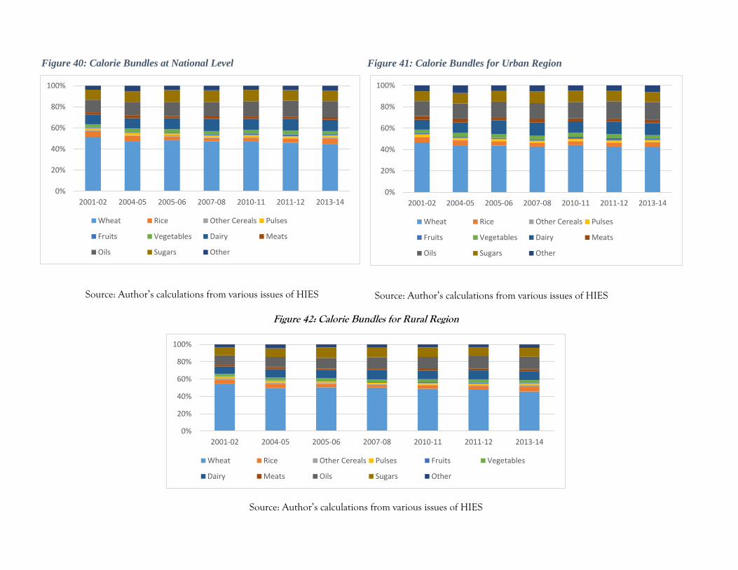
Source: Author’s calculations from various issues of HIES

Source: Author’s calculations from various issues of HIES

Figure 42: Calorie Bundles for Rural Region

Source: Author’s calculations from various issues of HIES

0%

20%

40%

60%

80%

100%

2001-02 2004-05 2005-06 2007-08 2010-11 2011-12 2013-14

Wheat Rice Other Cereals Pulses Fruits Vegetables

Dairy Meats Oils Sugars Other

0%

20%

40%

60%

80%

100%

2001-02 2004-05 2005-06 2007-08 2010-11 2011-12 2013-14

Wheat Rice Other Cereals Pulses

Fruits Vegetables Dairy Meats

Oils Sugars Other

0%

20%

40%

60%

80%

100%

2001-02 2004-05 2005-06 2007-08 2010-11 2011-12 2013-14

Wheat Rice Other Cereals Pulses

Fruits Vegetables Dairy Meats

Oils Sugars Other

Figure 40: Calorie Bundles at National Level Figure 41: Calorie Bundles for Urban Region

Source: Author’s calculations from various issues of HIES

Source: Author’s calculations from various issues of HIES

Figure 45: Calorie Bundles for KPK

Source: Author’s calculations from various issues of HIES Source: Author’s calculations from various issues of HIES

0

20

40

60

80

100

2001-02 2004-05 2005-06 2007-08 2010-11 2011-12 2013-14

Wheat Rice Other Cereals Pulses

Fruits Vegetables Dairy Meats

Oils Sugars Other

0

20

40

60

80

100

2001-02 2004-05 2005-06 2007-08 2010-11 2011-12 2013-14

Wheat Rice Other Cereals Pulses

Fruits Vegetables Dairy Meats

Oils Sugars Other

0

20

40

60

80

100

2001-02 2004-05 2005-06 2007-08 2010-11 2011-12 2013-14

Wheat Rice Other Cereals Pulses

Fruits Vegetables Dairy Meats

Oils Sugars Other

0

20

40

60

80

100

2001-02 2004-05 2005-06 2007-08 2010-11 2011-12 2013-14

Wheat Rice Other Cereals Pulses

Fruits Vegetables Dairy Meats

Oils Sugars Other

Figure 43: Calorie Bundles for Punjab Figure 44: Calorie Bundles for Sindh

Figure 46: Calorie Bundles for Balochistan

Figure 47: Cost of Calories at National Level

Source: Author’s calculations from various issues of HIES

Source: Author’s calculations from various issues of HIES

Source: Author’s calculations from various issues of HIES

0.00

2.00

4.00

6.00

8.00

10.00

12.00

14.00

16.00

2001-02 2004-05 2005-06 2007-08 2010-11 2011-12 2013-14

0.00

2.00

4.00

6.00

8.00

10.00

12.00

14.00

16.00

2001-02 2004-05 2005-06 2007-08 2010-11 2011-12 2013-14

0.00

2.00

4.00

6.00

8.00

10.00

12.00

14.00

16.00

2001-02 2004-05 2005-06 2007-08 2010-11 2011-12 2013-14

Figure 48: Cost of Calories at Urban Level Figure 49: Cost of Calories for Rural Region

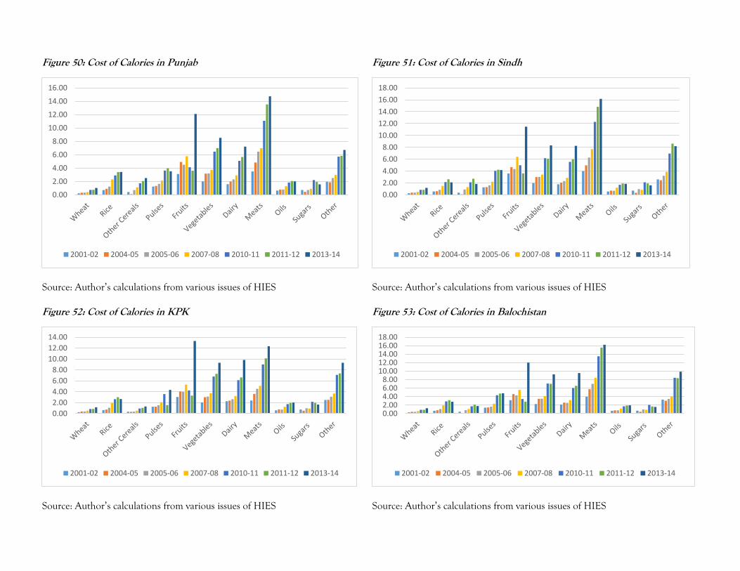
Figure 50: Cost of Calories in Punjab

Source: Author’s calculations from various issues of HIES

Figure 51: Cost of Calories in Sindh

Source: Author’s calculations from various issues of HIES

Figure 52: Cost of Calories in KPK

Source: Author’s calculations from various issues of HIES

Figure 53: Cost of Calories in Balochistan

Source: Author’s calculations from various issues of HIES

0.00

2.00

4.00

6.00

8.00

10.00

12.00

14.00

16.00

2001-02 2004-05 2005-06 2007-08 2010-11 2011-12 2013-14

0.00

2.00

4.00

6.00

8.00

10.00

12.00

14.00

16.00

18.00

2001-02 2004-05 2005-06 2007-08 2010-11 2011-12 2013-14

0.00

2.00

4.00

6.00

8.00

10.00

12.00

14.00

2001-02 2004-05 2005-06 2007-08 2010-11 2011-12 2013-14

0.002.004.006.008.00

10.0012.0014.0016.0018.00

2001-02 2004-05 2005-06 2007-08 2010-11 2011-12 2013-14

Table 8: Regression Coefficients (Alpha)

2001-02 2004-05 2005-06 2007-08 2010-11 2011-12 2013-14

alpha Coef. P>z Coef. P>z Coef. P>z Coef. P>z Coef. P>z Coef. P>z Coef. P>z

Wheat 0.36 0.00 0.57 0.00 0.34 0.00 0.26 0.00 0.30 0.00 0.40 0.00 0.35 0.00

Rice 0.06 0.00 0.01 0.29 0.02 0.08 0.05 0.00 0.05 0.00 0.01 0.06 0.01 0.16

Other Cereals 0.01 0.31 0.05 0.00 0.01 0.01 0.02 0.00 0.01 0.00 -0.01 0.00 0.01 0.02

Pulses 0.09 0.00 0.07 0.00 0.05 0.00 0.05 0.00 0.04 0.00 0.04 0.00 0.04 0.00

Fruits -0.02 0.20 0.01 0.52 0.03 0.00 0.04 0.00 0.04 0.00 0.01 0.00 0.03 0.00

Vegetables 0.25 0.00 0.26 0.00 0.25 0.00 0.20 0.00 0.18 0.00 0.23 0.00 0.23 0.00

Dairy 0.19 0.00 0.11 0.00 -0.03 0.39 0.08 0.00 0.16 0.00 0.15 0.00 0.13 0.00

Meats -0.14 0.00 -0.37 0.00 0.02 0.28 0.01 0.58 -0.06 0.00 -0.17 0.00 -0.13 0.00

Oils 0.10 0.00 0.11 0.00 0.08 0.00 0.08 0.00 0.07 0.00 0.17 0.00 0.10 0.00

Sugars 0.00 0.88 0.12 0.00 0.12 0.00 0.09 0.00 0.09 0.00 0.06 0.00 0.11 0.00

Other 0.09 0.00 0.07 0.00 0.11 0.00 0.13 0.00 0.14 0.00 0.10 0.00 0.12 0.00 Source: Author’s Own Calculation from Several issues of HIES

Table 9: Regression Coefficient (Beta)

2001-02 2004-05 2005-06 2007-08 2010-11 2011-12 2013-14

beta Coef. P>z Coef. P>z Coef. P>z Coef. P>z Coef. P>z Coef. P>z Coef. P>z

Wheat -0.04 0.00 -0.19 0.00 -0.05 0.00 -0.05 0.00 -0.08 0.00 -0.10 0.00 -0.04 0.00

Rice -0.01 0.04 0.02 0.05 0.02 0.03 0.00 0.36 0.01 0.00 0.03 0.00 0.02 0.00

Other Cereals 0.01 0.08 -0.03 0.00 0.00 0.72 0.00 0.02 0.00 0.02 0.01 0.00 0.00 0.17

Pulses -0.02 0.00 -0.01 0.00 -0.01 0.00 -0.01 0.00 -0.01 0.00 0.00 0.02 -0.01 0.00

Fruits 0.03 0.00 0.02 0.00 0.01 0.12 0.01 0.01 0.01 0.00 0.01 0.00 -0.01 0.00

Vegetables -0.03 0.00 -0.03 0.00 -0.06 0.00 -0.05 0.00 -0.04 0.00 -0.05 0.00 -0.04 0.00

Dairy -0.03 0.08 -0.02 0.29 0.18 0.00 0.16 0.00 0.09 0.00 0.05 0.00 0.08 0.00

Meats 0.06 0.00 0.27 0.00 -0.05 0.00 -0.03 0.00 0.05 0.00 0.08 0.00 0.04 0.00

Oils -0.02 0.00 -0.03 0.00 -0.01 0.03 0.00 0.31 -0.03 0.00 -0.06 0.00 -0.03 0.00

Sugars 0.04 0.00 -0.04 0.00 -0.05 0.00 -0.04 0.00 -0.03 0.00 0.00 0.32 -0.01 0.00

Other 0.02 0.00 0.04 0.00 0.02 0.03 0.03 0.00 0.02 0.00 0.04 0.00 0.00 0.27 Source: Author’s calculations from various issues of HIES

Table 10: Regression Coefficient (Gamma), Several Tables calculated by Author

2001-02 2004-05 2005-06 2007-08 2010-11 2011-12 2013-14

gamma Coef. P>z Coef. P>z Coef. P>z Coef. P>z Coef. P>z Coef. P>z Coef. P>z Wheat-Wheat 0.07 0.00 0.00 0.92 0.07 0.00 0.08 0.00 0.07 0.00 0.08 0.00 0.07 0.00 Rice-Wheat 0.01 0.00 0.03 0.00 0.01 0.00 0.00 0.02 0.02 0.00 0.02 0.00 0.00 0.70 Other Cereals-Wheat 0.01 0.00 -0.01 0.00 0.01 0.00 0.00 0.00 0.00 0.32 0.00 0.03 0.01 0.00 Pulses-Wheat 0.00 0.02 -0.01 0.00 0.00 0.01 0.00 0.17 -0.01 0.00 0.00 0.26 0.01 0.00 Fruits-Wheat -0.01 0.00 0.00 0.44 -0.01 0.00 -0.01 0.00 0.00 0.00 -0.01 0.00 -0.02 0.00 Vegetables-Wheat 0.00 0.07 -0.02 0.00 0.00 0.09 -0.01 0.00 -0.02 0.00 -0.02 0.00 -0.01 0.00 Dairy-Wheat -0.03 0.00 -0.03 0.00 -0.01 0.00 -0.03 0.00 -0.02 0.00 -0.03 0.00 0.00 0.08 Meats-Wheat -0.02 0.00 0.08 0.00 -0.03 0.00 -0.03 0.00 -0.03 0.00 -0.04 0.00 -0.04 0.00 Oils-Wheat -0.02 0.00 -0.03 0.00 -0.02 0.00 -0.01 0.00 -0.02 0.00 -0.02 0.00 -0.02 0.00 Sugars-Wheat 0.00 0.71 -0.02 0.00 -0.01 0.00 -0.01 0.00 -0.01 0.00 -0.01 0.00 -0.01 0.00 Other-Wheat 0.01 0.02 0.01 0.02 0.01 0.01 0.01 0.00 0.01 0.00 0.01 0.00 0.00 0.48

2001-02 2004-05 2005-06 2007-08 2010-11 2011-12 2013-14

Gamma Coef. P>z Coef. P>z Coef. P>z Coef. P>z Coef. P>z Coef. P>z Coef. P>z Rice-Rice -0.02 0.00 -0.03 0.00 -0.02 0.00 0.00 0.06 -0.01 0.00 -0.01 0.00 0.00 0.00 Other Cereals-Rice 0.00 0.77 0.00 0.50 0.00 0.00 0.00 0.76 0.00 0.48 0.00 0.82 -0.01 0.00 Pulses-Rice 0.00 1.00 0.00 0.52 0.00 0.00 0.00 0.00 0.00 0.71 0.00 0.80 0.00 0.00 Fruits-Rice 0.01 0.00 0.01 0.00 0.01 0.00 0.00 0.00 0.00 0.00 0.00 0.00 0.01 0.00 Vegetables-Rice 0.00 0.65 -0.01 0.00 0.01 0.00 0.00 0.19 0.00 0.03 0.00 0.95 0.00 0.00 Dairy-Rice -0.01 0.00 0.01 0.00 -0.01 0.02 -0.01 0.00 0.00 0.22 0.01 0.00 0.00 0.00 Meats-Rice 0.02 0.00 -0.01 0.19 -0.01 0.01 0.00 0.01 0.00 0.04 0.00 0.02 0.00 0.06 Oils-Rice -0.01 0.00 0.00 0.02 0.00 0.77 0.00 0.07 -0.01 0.00 0.00 0.43 0.01 0.00 Sugars-Rice 0.00 0.13 0.01 0.00 0.00 0.70 -0.01 0.00 0.00 0.03 -0.01 0.00 -0.02 0.00 Others-Rice 0.00 0.98 0.00 0.48 0.00 0.31 0.00 0.00 0.01 0.00 -0.01 0.00 0.01 0.00

2001-02 2004-05 2005-06 2007-08 2010-11 2011-12 2013-14

Gamma Coef. P>z Coef. P>z Coef. P>z Coef. P>z Coef. P>z Coef. P>z Coef. P>z Other Cereals-Other Cereals -0.01 0.00 0.00 0.00 -0.01 0.00 -0.01 0.00 0.00 0.00 0.00 0.00 -0.01 0.00 Pulses-Other Cereals 0.00 0.78 0.00 0.02 0.00 0.00 0.00 0.00 0.00 0.53 0.00 0.00 0.00 0.00 Fruits-Other Cereals 0.00 0.19 0.00 0.00 0.00 0.01 0.00 0.15 0.00 0.00 0.00 0.02 0.00 0.00 Vegetables-Other Cereals 0.00 0.00 0.00 0.00 0.00 0.10 0.00 0.00 0.00 0.48 0.00 0.55 0.00 0.00 Dairy-Other Cereals 0.00 0.05 0.00 0.87 0.00 0.06 0.00 0.12 0.00 0.11 0.00 0.08 0.00 0.17 Meats-Other Cereals 0.00 0.00 0.01 0.00 0.00 0.18 0.00 0.00 0.00 0.00 0.00 0.00 0.01 0.00 Oils-Other Cereals 0.00 0.00 0.00 0.05 0.00 0.72 0.00 0.00 0.00 0.94 0.01 0.00 0.00 0.00 Sugars-Other Cereals 0.00 0.00 0.00 0.00 0.00 0.83 0.00 0.05 0.00 0.01 0.00 0.03 0.00 0.00 Other-Other Cereals 0.00 0.03 0.00 0.00 0.00 0.00 0.00 0.00 0.00 0.00 0.00 0.00 0.01 0.00 Pulses-Pulses 0.01 0.00 0.01 0.00 0.02 0.00 0.01 0.00 0.02 0.00 0.01 0.00 0.01 0.00 Fruits-Pulses 0.00 0.16 0.00 0.81 0.00 0.00 0.00 0.01 0.00 0.00 0.00 0.00 0.00 0.82 Vegetables-Pulses 0.00 0.01 0.00 0.34 0.00 0.07 0.00 0.01 0.00 0.05 0.00 0.11 0.00 0.00 Dairy-Pulses 0.00 0.04 0.00 0.23 0.00 0.76 0.00 0.81 0.00 0.00 0.00 0.00 0.00 0.01 Meats-Pulses 0.00 0.02 0.00 0.35 -0.01 0.00 -0.01 0.00 -0.01 0.00 -0.01 0.00 0.00 0.00 Oils-Pulses 0.00 0.55 0.00 0.00 0.00 0.00 -0.01 0.00 0.00 0.00 0.00 0.35 0.00 0.00 Sugars-Pulses 0.00 0.82 0.00 0.00 0.00 0.00 0.00 0.14 0.00 0.00 0.00 0.00 0.00 0.00 Others-Pulses 0.00 0.33 0.00 0.08 0.00 0.03 0.00 0.41 0.00 0.01 0.00 0.00 0.00 0.00

2001-02 2004-05 2005-06 2007-08 2010-11 2011-12 2013-14

gamma Coef. P>z Coef. P>z Coef. P>z Coef. P>z Coef. P>z Coef. P>z Coef. P>z Fruits-Fruits 0.01 0.00 0.01 0.00 0.02 0.00 0.01 0.00 0.00 0.00 0.00 0.00 0.01 0.00 Vegetables-Fruits 0.00 0.37 0.00 0.51 0.00 0.00 -0.01 0.00 0.00 0.00 0.00 0.00 -0.01 0.00 Dairy-Fruits 0.01 0.00 0.00 0.28 0.00 0.62 0.00 0.02 0.00 0.00 0.00 0.05 0.00 0.00 Meats-Fruits 0.00 0.35 -0.01 0.00 0.00 0.12 -0.01 0.00 0.00 0.00 0.00 0.00 0.01 0.00 Oils-Fruits 0.00 0.07 0.00 0.13 -0.01 0.00 -0.01 0.00 0.00 0.00 0.00 0.00 -0.01 0.00 Sugars-Fruits -0.01 0.00 0.00 0.75 0.00 0.00 0.01 0.00 0.00 0.00 0.00 0.00 0.00 0.00 Others-Fruits 0.00 0.29 -0.01 0.00 0.00 0.11 0.00 0.34 0.00 0.17 0.00 0.28 0.00 0.92 Vegetables-Vegetables 0.04 0.00 0.06 0.00 0.05 0.00 0.05 0.00 0.05 0.00 0.05 0.00 0.05 0.00 Dairy--Vegetables -0.01 0.00 0.00 0.16 0.01 0.03 0.01 0.00 0.00 0.54 0.00 0.53 0.00 0.01 Meats--Vegetables -0.01 0.00 0.01 0.43 -0.02 0.00 -0.02 0.00 -0.02 0.00 -0.02 0.00 -0.02 0.00 Oils-Vegetables -0.02 0.00 -0.02 0.00 -0.01 0.00 -0.01 0.00 -0.01 0.00 -0.01 0.00 -0.01 0.00 Sugars-Vegetables 0.00 0.06 -0.01 0.00 -0.01 0.00 -0.01 0.00 0.00 0.00 -0.01 0.00 0.00 0.01 Others-Vegetables 0.00 0.00 0.00 0.01 0.00 0.01 0.00 0.03 0.00 0.00 0.01 0.00 0.00 0.00 Dairy-Dairy 0.00 0.52 -0.02 0.00 0.01 0.10 0.05 0.00 0.03 0.00 0.03 0.00 -0.01 0.00 Meats-Dairy 0.02 0.00 0.04 0.01 0.00 0.81 0.00 0.74 0.00 0.28 0.00 0.70 0.01 0.00 Oils-Dairy 0.00 0.48 0.00 0.87 0.00 0.14 -0.01 0.00 0.00 0.71 -0.01 0.00 0.00 0.06 Sugars-Dairy 0.01 0.05 0.00 0.19 0.00 0.18 -0.02 0.00 -0.02 0.00 -0.02 0.00 0.00 0.48 Others-Dairy 0.01 0.00 0.01 0.00 0.00 0.11 0.00 0.20 0.00 0.39 0.01 0.01 0.00 0.00 Meats-Meats 0.08 0.00 -0.11 0.00 0.09 0.00 0.09 0.00 0.10 0.00 0.11 0.00 0.11 0.00 Oils-Meats -0.01 0.00 0.01 0.20 -0.01 0.00 -0.02 0.00 -0.02 0.00 -0.02 0.00 -0.03 0.00 Sugars-Meats -0.04 0.00 0.02 0.00 -0.01 0.00 0.00 0.10 0.00 0.06 0.00 0.83 -0.01 0.00 Others-Meats -0.02 0.00 -0.03 0.00 0.00 0.83 -0.01 0.00 -0.01 0.00 -0.02 0.00 -0.03 0.00 Oils-Oils 0.07 0.00 0.06 0.00 0.05 0.00 0.07 0.00 0.08 0.00 0.05 0.00 0.06 0.00 Sugars-Oils -0.01 0.00 -0.01 0.00 0.00 0.00 -0.01 0.00 -0.01 0.00 -0.01 0.00 -0.01 0.00 Others--Oils 0.00 0.01 0.00 0.36 0.00 0.55 0.00 0.55 0.00 0.37 0.00 0.08 0.00 0.16 Sugars-Sugars 0.04 0.00 0.01 0.00 0.04 0.00 0.04 0.00 0.04 0.00 0.04 0.00 0.05 0.00 Others-Sugars 0.01 0.00 0.01 0.00 0.00 0.01 0.01 0.00 0.00 0.34 0.00 0.00 0.00 0.60 Others-Others 0.00 0.04 0.00 0.64 -0.01 0.01 -0.02 0.00 -0.01 0.00 0.00 0.34 0.00 0.00

Table 11: Regression Coefficients (Lambda)

2001-02 2004-05 2005-06 2007-08 2010-11 2011-12 2013-14

lambda Coef. P>z Coef. P>z Coef. P>z Coef. P>z Coef. P>z Coef. P>z Coef. P>z

Wheat 0.00 0.29 0.02 0.00 0.00 0.63 0.00 0.27 0.00 0.15 0.01 0.00 0.01 0.00

Rice 0.00 0.01 0.00 0.14 0.00 0.03 0.00 0.12 0.00 0.00 0.00 0.00 0.00 0.00

Other Cereals 0.00 0.00 0.00 0.00 0.00 0.17 0.00 0.75 0.00 0.00 0.00 0.00 0.00 0.00

Pulses 0.00 0.00 0.00 0.09 0.00 0.23 0.00 0.07 0.00 0.01 0.00 0.00 0.00 0.00

Fruits 0.00 0.01 0.00 0.01 0.00 0.76 0.00 0.02 0.00 0.03 0.00 0.33 0.00 0.00

Vegetables 0.00 0.10 0.00 0.96 0.01 0.00 0.01 0.00 0.00 0.00 0.00 0.00 0.00 0.00

Dairy 0.01 0.00 0.01 0.00 -0.02 0.00 -0.02 0.00 0.00 0.00 0.01 0.00 -0.01 0.00

Meats 0.00 0.00 -0.04 0.00 0.01 0.00 0.01 0.00 0.00 0.00 -0.01 0.00 0.00 0.00

Oils 0.00 0.19 0.00 0.09 0.00 0.75 0.00 0.02 0.00 0.00 0.01 0.00 0.00 0.00

Sugars -0.01 0.00 0.01 0.00 0.01 0.00 0.00 0.11 0.00 0.00 0.00 0.00 0.00 0.00

Other 0.00 0.73 0.00 0.01 0.00 0.45 0.00 0.05 0.00 0.00 0.00 0.00 0.00 0.00

Table 12: Regression Dummy for Region

2001-02 2004-05 2005-06 2007-08 2010-11 2011-12 2013-14

Region Coef. P>z Coef. P>z Coef. P>z Coef. P>z Coef. P>z Coef. P>z Coef. P>z

Wheat 0.02 0.00 0.01 0.00 0.01 0.00 0.02 0.00 0.02 0.00 0.01 0.00 -0.01 0.00

Rice 0.00 0.00 0.00 0.93 0.00 0.00 0.00 0.03 0.00 0.99 0.00 0.00 0.00 0.37

Other Cereals 0.00 0.00 0.00 0.00 0.00 0.00 0.00 0.00 0.00 0.00 0.00 0.00 0.00 0.00

Pulses 0.00 0.00 0.00 0.00 0.00 0.48 0.00 0.01 0.00 0.00 0.00 0.73 0.00 0.02

Fruits 0.00 0.00 0.00 0.00 0.00 0.00 -0.01 0.00 0.00 0.00 0.00 0.00 0.00 0.00

Vegetables 0.01 0.00 0.00 0.00 0.00 0.65 0.00 0.68 0.00 0.00 0.00 0.00 0.00 0.00

Dairy -0.01 0.00 0.00 0.00 0.01 0.00 0.01 0.00 0.00 0.55 0.00 0.00 0.00 0.53

Meats -0.01 0.00 -0.01 0.00 -0.01 0.00 -0.02 0.00 -0.02 0.00 -0.01 0.00 0.00 0.00

Oils 0.00 0.00 0.00 0.00 0.00 0.03 0.00 0.83 0.00 0.00 0.00 0.18 0.00 0.79

Sugars 0.01 0.00 0.00 0.00 0.00 0.00 0.01 0.00 0.01 0.00 0.00 0.00 0.00 0.00

Other -0.01 0.00 -0.01 0.00 -0.01 0.00 -0.01 0.00 -0.01 0.00 -0.01 0.00 0.01 0.00

Table 13: Regression Dummy for Province

2001-02 2004-05 2005-06 2007-08 2010-11 2011-12 2013-14

Province Coef. P>z Coef. P>z Coef. P>z Coef. P>z Coef. P>z Coef. P>z Coef. P>z

Wheat 0.00 0.00 0.00 0.00 0.00 0.00 0.01 0.00 0.01 0.00 0.01 0.00 0.00 0.01

Rice 0.00 0.00 0.00 0.00 0.00 0.65 0.00 0.10 0.00 0.00 0.00 0.26 0.00 0.00

Other Cereals 0.00 0.00 0.00 0.00 0.00 0.00 0.00 0.00 0.00 0.00 0.00 0.00 0.00 0.00

Pulses 0.00 0.00 0.00 0.41 0.00 0.49 0.00 0.00 0.00 0.00 0.00 0.00 0.00 0.02

Fruits 0.00 0.03 0.00 0.00 0.00 0.07 0.00 0.00 0.00 0.00 0.00 0.00 0.00 0.00

Vegetables 0.00 0.00 0.00 0.00 0.00 0.00 0.00 0.00 0.01 0.00 0.00 0.00 0.00 0.00

Dairy 0.00 0.01 -0.01 0.00 -0.01 0.00 -0.02 0.00 -0.03 0.00 -0.02 0.00 -0.01 0.00

Meats 0.00 0.00 0.00 0.00 0.01 0.00 0.01 0.00 0.00 0.95 0.00 0.42 0.00 0.05

Oils 0.00 0.00 0.00 0.00 0.00 0.48 0.00 0.00 0.00 0.00 0.00 0.00 0.00 0.00

Sugars 0.00 0.27 0.00 0.00 0.00 0.00 0.01 0.00 0.01 0.00 0.01 0.00 0.00 0.00

Other 0.00 0.02 0.00 0.00 0.00 0.00 0.00 0.83 0.00 0.00 0.00 0.34 0.00 0.00

Table 14: Expenditure Elasticities at National Level

2001-02 2004-05 2005-06 2007-08 2010-11 2011-12 2013-14

Wheat 0.7 1.2 0.7 0.7 0.7 1.0 1.1

Rice 1.3 0.8 0.5 1.5 1.2 0.6 0.6

Other Cereals -0.5 3.3 0.0 1.2 -0.1 -1.1 2.3

Pulses 0.9 0.7 0.8 1.0 0.7 0.6 1.3

Fruits 1.0 0.8 1.3 1.7 1.3 1.3 1.2

Vegetables 0.8 0.7 1.2 1.5 0.8 1.0 1.0

Dairy 1.3 1.5 0.7 0.6 1.3 1.3 1.0

Meats 1.1 0.1 1.9 2.2 1.2 0.9 1.1

Oils 0.8 0.9 0.8 0.6 0.9 1.0 1.0

Sugars 0.8 1.2 1.3 1.0 0.7 0.4 1.0

Other 1.1 0.9 0.9 0.8 1.1 0.8 0.8

Table 15: Expenditure Elasticities for Urban Region

2001-02 2004-05 2005-06 2007-08 2010-11 2011-12 2013-14

Wheat 0.5 1.0 0.5 0.5 0.5 1.0 1.1

Rice 1.2 0.9 0.5 1.4 1.2 0.6 0.6

Other Cereals 0.6 2.9 -0.3 1.1 -0.1 -1.1 2.2

Pulses 0.8 0.7 0.8 1.0 0.7 0.6 1.3

Fruits 1.2 0.9 1.3 1.7 1.4 1.3 1.2

Vegetables 0.7 0.7 1.2 1.4 0.8 1.0 1.0

Dairy 1.3 1.5 0.8 0.6 1.3 1.3 1.0

Meats 1.2 0.6 1.8 2.1 1.3 1.0 1.1

Oils 0.8 0.9 0.8 0.6 0.8 1.0 1.0

Sugars 0.8 1.2 1.2 0.9 0.6 0.3 1.0

Other 1.1 1.0 1.0 0.9 1.1 0.9 0.9

Table 16: Expenditure Elasticities for Rural Region

2001-02 2004-05 2005-06 2007-08 2010-11 2011-12 2013-14

Wheat 0.8 1.3 0.8 0.8 0.8 1.1 1.1

Rice 1.4 0.8 0.5 1.5 1.1 0.6 0.6

Other Cereals -0.5 3.5 0.2 1.3 -0.1 -1.1 2.3

Pulses 1.0 0.8 0.8 1.0 0.7 0.6 1.3

Fruits 0.9 0.7 1.3 1.8 1.3 1.3 1.2

Vegetables 0.8 0.8 1.2 1.5 0.8 1.1 1.0

Dairy 1.3 1.5 0.7 0.6 1.3 1.3 1.0

Meats 1.0 -0.3 2.0 2.3 1.1 0.9 1.0

Oils 0.8 0.9 0.8 0.6 0.9 1.0 1.0

Sugars 0.8 1.3 1.3 1.1 0.7 0.5 1.0

Other 1.1 0.8 0.9 0.6 1.1 0.7 0.8

Table 17: Expenditure Elasticities for Punjab

2001-02 2004-05 2005-06 2007-08 2010-11 2011-12 2013-14

Wheat 0.7 1.1 0.6 0.6 0.6 0.9 1.1

Rice 1.4 0.9 0.3 1.6 1.3 0.7 0.6

Other Cereals -1.4 3.5 -0.6 1.1 -0.4 -1.5 2.6

Pulses 1.0 0.7 0.8 1.0 0.6 0.5 1.3

Fruits 1.0 0.8 1.3 1.7 1.3 1.4 1.1

Vegetables 0.8 0.7 1.2 1.5 0.7 1.0 1.0

Dairy 1.3 1.5 0.8 0.7 1.3 1.3 1.0

Meats 1.0 0.0 2.0 2.3 1.2 1.0 1.1

Oils 0.9 0.9 0.8 0.6 0.8 1.0 1.0

Sugars 0.7 1.2 1.3 0.9 0.6 0.3 1.0

Other 1.1 0.9 0.9 0.7 1.1 0.8 0.9

Table 18: Expenditure Elasticities for Sindh

2001-02 2004-05 2005-06 2007-08 2010-11 2011-12 2013-14

Wheat 0.5 1.1 0.7 0.7 0.7 1.0 1.2

Rice 1.2 0.9 0.7 1.3 1.1 0.8 0.7

Other Cereals -0.6 3.0 0.1 1.2 0.2 -0.6 2.0

Pulses 0.8 0.7 0.8 1.0 0.7 0.6 1.3

Fruits 1.1 0.8 1.3 1.9 1.4 1.3 1.2

Vegetables 0.7 0.7 1.2 1.5 0.8 1.0 1.0

Dairy 1.3 1.5 0.8 0.6 1.2 1.3 1.0

Meats 1.1 0.5 1.8 2.1 1.2 0.9 1.0

Oils 0.8 0.9 0.8 0.6 0.9 1.0 1.0

Sugars 0.8 1.2 1.3 1.0 0.7 0.5 1.0

Other 1.1 0.9 0.9 0.8 1.1 0.8 0.9

Table 19: Expenditure Elasticities for KPK

2001-02 2004-05 2005-06 2007-08 2010-11 2011-12 2013-14

Wheat 0.8 1.2 0.8 0.8 0.9 1.2 1.0

Rice 1.4 0.7 0.4 1.5 1.1 0.3 0.6

Other Cereals 0.3 2.7 0.6 1.4 0.5 -0.7 2.1

Pulses 0.9 0.8 0.8 1.0 0.9 0.8 1.1

Fruits 1.0 0.7 1.2 1.6 1.2 1.2 1.1

Vegetables 0.8 0.7 1.2 1.4 0.9 1.6 0.9

Dairy 1.3 1.5 0.6 0.5 1.2 1.3 1.1

Meats 1.2 -0.2 2.0 2.3 1.1 0.8 1.1

Oils 0.8 0.9 0.8 0.6 0.9 1.2 0.9

Sugars 0.9 1.2 1.2 1.1 0.8 0.6 0.9

Other 1.1 0.8 0.9 0.7 1.1 0.7 0.8

Table 20: Expenditure Elasticities for Balochistan

2001-02 2004-05 2005-06 2007-08 2010-11 2011-12 2013-14

Wheat 0.8 1.2 0.8 0.9 1.0 1.4 1.4

Rice 1.1 0.8 0.7 1.5 0.8 -0.1 0.0

Other Cereals 0.3 3.8 0.8 1.5 -0.4 -2.5 3.0

Pulses 0.8 0.8 0.8 1.0 0.9 0.8 1.6

Fruits 1.1 0.7 1.3 1.7 1.3 1.3 1.4

Vegetables 0.8 0.8 1.1 1.2 1.0 1.3 1.4

Dairy 1.4 1.6 0.5 -0.1 1.1 1.4 0.5

Meats 1.1 0.5 1.6 1.8 1.0 0.7 0.8

Oils 0.8 0.9 0.8 0.6 1.0 1.3 1.2

Sugars 0.9 1.3 1.3 1.2 0.7 0.4 1.3

Other 1.1 0.9 0.9 0.7 1.2 0.5 0.6

Table 21: Own Price Elasticities at National Level

2001-02 2004-05 2005-06 2007-08 2010-11 2011-12 2013-14

Wheat -0.23 -0.16 -0.29 -0.16 -0.30 -0.01 -0.30

Rice -2.05 -2.31 -1.94 -1.12 -1.56 -1.42 -1.09

Other Cereals -2.83 -0.98 -2.92 -2.24 -1.91 -1.38 -2.91

Pulses -0.50 -0.18 0.25 -0.16 -0.11 -0.46 -0.59

Fruits -0.63 -0.43 -0.32 -0.43 -0.80 -0.88 -0.38

Vegetables -0.41 -0.26 -0.28 -0.11 -0.28 -0.26 -0.34

Dairy -0.97 -1.09 -0.46 -0.33 -0.88 -0.93 -1.00

Meats 0.23 0.73 0.06 0.06 0.27 0.47 0.51

Oils -0.07 -0.21 -0.29 -0.25 -0.09 -0.40 -0.18

Sugars -0.17 -0.74 -0.39 -0.14 -0.39 -0.17 0.10

Other -0.96 -0.93 -1.04 -1.14 -1.10 -0.95 -0.92

Table 22: Own Price Elasticities at Urban Level

2001-02 2004-05 2005-06 2007-08 2010-11 2011-12 2013-14

Wheat -0.02 0.01 -0.13 0.02 -0.17 0.16 -0.17

Rice -1.96 -2.18 -1.90 -1.12 -1.55 -1.41 -1.09

Other Cereals -3.21 -1.01 -3.05 -2.29 -1.93 -1.38 -3.04

Pulses -0.51 -0.16 0.27 -0.10 -0.10 -0.46 -0.59

Fruits -0.69 -0.52 -0.42 -0.52 -0.82 -0.89 -0.49

Vegetables -0.40 -0.24 -0.26 -0.11 -0.27 -0.25 -0.33

Dairy -0.99 -1.10 -0.50 -0.38 -0.88 -0.92 -1.00

Meats 0.02 0.25 -0.12 -0.10 0.11 0.27 0.32

Oils -0.09 -0.19 -0.28 -0.22 -0.04 -0.38 -0.18

Sugars -0.06 -0.71 -0.32 -0.04 -0.33 -0.11 0.25

Other -0.97 -0.94 -1.04 -1.13 -1.09 -0.95 -0.93

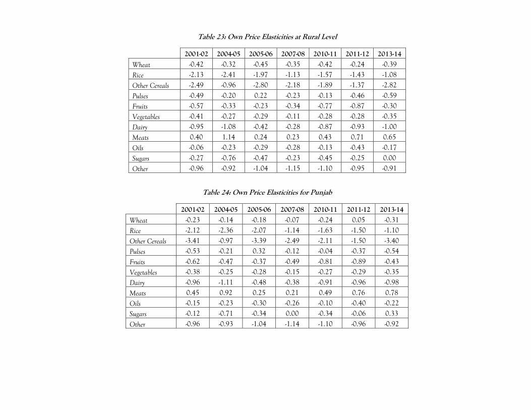
Table 23: Own Price Elasticities at Rural Level

2001-02 2004-05 2005-06 2007-08 2010-11 2011-12 2013-14

Wheat -0.42 -0.32 -0.45 -0.35 -0.42 -0.24 -0.39

Rice -2.13 -2.41 -1.97 -1.13 -1.57 -1.43 -1.08

Other Cereals -2.49 -0.96 -2.80 -2.18 -1.89 -1.37 -2.82

Pulses -0.49 -0.20 0.22 -0.23 -0.13 -0.46 -0.59

Fruits -0.57 -0.33 -0.23 -0.34 -0.77 -0.87 -0.30

Vegetables -0.41 -0.27 -0.29 -0.11 -0.28 -0.28 -0.35

Dairy -0.95 -1.08 -0.42 -0.28 -0.87 -0.93 -1.00

Meats 0.40 1.14 0.24 0.23 0.43 0.71 0.65

Oils -0.06 -0.23 -0.29 -0.28 -0.13 -0.43 -0.17

Sugars -0.27 -0.76 -0.47 -0.23 -0.45 -0.25 0.00

Other -0.96 -0.92 -1.04 -1.15 -1.10 -0.95 -0.91

Table 24: Own Price Elasticities for Punjab

2001-02 2004-05 2005-06 2007-08 2010-11 2011-12 2013-14

Wheat -0.23 -0.14 -0.18 -0.07 -0.24 0.05 -0.31

Rice -2.12 -2.36 -2.07 -1.14 -1.63 -1.50 -1.10

Other Cereals -3.41 -0.97 -3.39 -2.49 -2.11 -1.50 -3.40

Pulses -0.53 -0.21 0.32 -0.12 -0.04 -0.37 -0.54

Fruits -0.62 -0.47 -0.37 -0.49 -0.81 -0.89 -0.43

Vegetables -0.38 -0.25 -0.28 -0.15 -0.27 -0.29 -0.35

Dairy -0.96 -1.11 -0.48 -0.38 -0.91 -0.96 -0.98

Meats 0.45 0.92 0.25 0.21 0.49 0.76 0.78

Oils -0.15 -0.23 -0.30 -0.26 -0.10 -0.40 -0.22

Sugars -0.12 -0.71 -0.34 0.00 -0.34 -0.06 0.33

Other -0.96 -0.93 -1.04 -1.14 -1.10 -0.96 -0.92

Table 25: Own Price Elasticities for Sindh

2001-02 2004-05 2005-06 2007-08 2010-11 2011-12 2013-14

Wheat 0.14 0.04 -0.32 -0.12 -0.27 0.05 -0.38

Rice -1.70 -1.98 -1.58 -1.07 -1.40 -1.30 -1.06

Other Cereals -3.22 -1.00 -2.87 -2.11 -1.76 -1.31 -2.80

Pulses -0.44 -0.07 0.24 -0.06 -0.11 -0.49 -0.52

Fruits -0.71 -0.39 -0.26 -0.33 -0.77 -0.86 -0.24

Vegetables -0.40 -0.23 -0.21 0.07 -0.18 -0.18 -0.21

Dairy -0.98 -1.09 -0.51 -0.33 -0.89 -0.93 -0.97

Meats -0.26 0.12 -0.11 -0.08 0.01 0.14 0.20

Oils -0.01 -0.15 -0.27 -0.26 -0.08 -0.38 -0.13

Sugars 0.05 -0.71 -0.36 -0.10 -0.40 -0.23 0.01

Other -0.97 -0.94 -1.03 -1.12 -1.09 -0.96 -0.92

Table 26: Own Price Elasticities for KPK

2001-02 2004-05 2005-06 2007-08 2010-11 2011-12 2013-14

Wheat -0.43 -0.39 -0.44 -0.37 -0.42 -0.27 -0.49

Rice -2.30 -2.62 -2.22 -1.15 -1.66 -1.43 -1.11

Other Cereals -2.09 -0.99 -2.14 -1.95 -1.63 -1.22 -2.43

Pulses -0.45 -0.21 0.18 -0.39 -0.22 -0.60 -0.66

Fruits -0.61 -0.36 -0.33 -0.50 -0.82 -0.89 -0.49

Vegetables -0.46 -0.24 -0.32 -0.20 -0.38 -0.32 -0.37

Dairy -0.96 -1.07 -0.40 -0.37 -0.83 -0.88 -0.99

Meats 0.41 1.25 0.07 0.08 0.32 0.39 0.65

Oils -0.03 -0.27 -0.27 -0.23 -0.12 -0.43 -0.19

Sugars -0.47 -0.81 -0.55 -0.29 -0.52 -0.36 -0.14

Other -0.96 -0.92 -1.04 -1.15 -1.11 -0.93 -0.92

Table 27: Own Price Elasticities for Balochistan

2001-02 2004-05 2005-06 2007-08 2010-11 2011-12 2013-14

Wheat -0.53 -0.33 -0.46 -0.43 -0.54 -0.35 -0.50

Rice -1.63 -2.20 -1.82 -1.16 -1.50 -1.28 -0.92

Other Cereals -2.38 -1.00 -2.56 -1.82 -1.65 -1.13 -2.89

Pulses -0.58 -0.22 0.02 -0.32 -0.42 -0.65 -0.71

Fruits -0.66 -0.34 -0.27 -0.28 -0.60 -0.85 -0.28

Vegetables -0.50 -0.36 -0.42 -0.44 -0.44 -0.39 -0.35

Dairy -0.96 -1.06 -0.31 0.19 -0.66 -0.75 -0.80

Meats -0.27 2.03 -0.35 -0.38 -0.29 -0.02 -0.09

Oils -0.03 -0.18 -0.31 -0.21 0.03 -0.49 -0.29

Sugars -0.12 -0.76 -0.43 -0.35 -0.43 -0.19 0.00

Other -0.95 -0.93 -1.04 -1.18 -1.10 -0.85 -0.83

Syed Masroor Hussain Zaidi

Table 28: Elasticity Matrices for Punjab

Marshallian Elasticity Matrix for Punjab

Wheat Rice Other Cereals Pulses Fruits Vegetables Dairy Meats Oils Sugars Other

Wheat -0.51 0.06 0.03 0.00 -0.05 -0.03 -0.10 -0.22 -0.07 -0.03 0.04 Rice 0.33 -1.44 -0.01 0.04 0.16 -0.04 0.05 0.07 -0.11 -0.14 0.10 Other Cereals 1.77 -0.14 -3.04 -0.46 0.25 -0.11 0.55 -0.77 0.80 -0.10 1.11 Pulses -0.01 0.06 -0.05 -0.52 -0.01 0.04 0.02 -0.32 -0.07 -0.07 0.03 Fruits -0.37 0.17 0.02 -0.01 -0.65 -0.15 -0.02 0.01 -0.16 0.00 -0.06 Vegetables -0.06 -0.01 0.00 0.01 -0.04 -0.44 -0.08 -0.19 -0.09 -0.05 -0.03 Dairy -0.10 0.00 0.00 0.00 0.00 -0.04 -0.87 -0.03 -0.03 -0.05 0.00 Meats -0.50 0.02 -0.03 -0.11 0.00 -0.24 -0.14 0.29 -0.28 -0.09 -0.17 Oils -0.12 -0.02 0.02 -0.02 -0.03 -0.07 0.00 -0.18 -0.40 -0.07 0.01 Sugars -0.07 -0.09 -0.01 -0.03 0.02 -0.07 -0.14 -0.07 -0.12 -0.40 0.08 Other 0.05 0.04 0.03 0.01 -0.01 -0.02 0.06 -0.10 0.00 0.05 -1.02

Hicksian Elasticity Matrix for Punjab

Wheat Rice Other Cereals Pulses Fruits Vegetables Dairy Meats Oils Sugars Other

Wheat -0.35 0.09 0.03 0.02 -0.03 0.06 0.13 -0.15 0.03 0.04 0.13 Rice 0.50 -1.41 -0.01 0.07 0.19 0.06 0.31 0.15 0.01 -0.06 0.20 Other Cereals 1.82 -0.13 -3.03 -0.46 0.26 -0.07 0.61 -0.75 0.82 -0.10 1.14 Pulses 0.14 0.09 -0.04 -0.50 0.02 0.13 0.26 -0.24 0.03 0.00 0.13 Fruits -0.16 0.21 0.02 0.02 -0.62 -0.03 0.31 0.11 -0.02 0.09 0.06 Vegetables 0.10 0.03 0.00 0.04 -0.01 -0.34 0.18 -0.11 0.02 0.02 0.07 Dairy 0.09 0.04 0.01 0.03 0.04 0.07 -0.57 0.06 0.10 0.03 0.12 Meats -0.29 0.06 -0.03 -0.08 0.03 -0.12 0.19 0.40 -0.14 0.00 -0.04 Oils 0.03 0.01 0.02 0.01 0.00 0.01 0.23 -0.10 -0.30 0.00 0.10 Sugars 0.08 -0.06 -0.01 0.00 0.04 0.02 0.10 0.01 -0.02 -0.34 0.17 Other 0.21 0.07 0.03 0.03 0.02 0.07 0.30 -0.02 0.10 0.12 -0.92

Substitutes

Compliments

No Relation

Elasticity Matrix

Marshallian Hicksian

No Relation 11 6 Substitutes 29 77 Compliments 70 27

Table 29: Elasticity Matrices for Sindh

Marshallian Elasticity Matrix for Sindh

Wheat Rice Other Cereals Pulses Fruits Vegetables Dairy Meats Oils Sugars Other

Wheat -0.48 0.07 0.03 0.00 -0.06 -0.04 -0.11 -0.25 -0.08 -0.03 0.03 Rice 0.16 -1.20 -0.01 0.02 0.08 -0.01 0.03 0.03 -0.05 -0.07 0.06 Other Cereals 1.68 -0.06 -2.88 -0.36 0.18 0.02 0.49 -0.89 0.66 -0.08 0.85 Pulses -0.02 0.07 -0.06 -0.42 -0.01 0.05 0.02 -0.39 -0.09 -0.09 0.03 Fruits -0.50 0.22 0.03 -0.01 -0.53 -0.21 -0.01 0.00 -0.21 0.02 -0.09 Vegetables -0.07 -0.01 0.00 0.01 -0.04 -0.42 -0.07 -0.21 -0.10 -0.06 -0.03 Dairy -0.10 0.00 0.00 0.00 0.00 -0.03 -0.85 -0.03 -0.02 -0.06 0.00 Meats -0.38 0.01 -0.02 -0.08 0.00 -0.18 -0.09 -0.05 -0.21 -0.07 -0.13 Oils -0.14 -0.03 0.02 -0.02 -0.03 -0.09 0.00 -0.20 -0.32 -0.08 0.00 Sugars -0.08 -0.07 -0.01 -0.03 0.01 -0.07 -0.12 -0.08 -0.11 -0.47 0.07 Other 0.04 0.03 0.02 0.01 -0.01 -0.02 0.05 -0.09 0.00 0.04 -1.01

Hicksian Elasticity Matrix for Sindh

Wheat Rice Other Cereals Pulses Fruits Vegetables Dairy Meats Oils Sugars Other

Wheat -0.33 0.13 0.03 0.02 -0.04 0.05 0.10 -0.14 0.01 0.04 0.14 Rice 0.31 -1.13 0.00 0.04 0.10 0.08 0.25 0.14 0.05 0.00 0.17 Other Cereals 1.75 -0.04 -2.87 -0.36 0.19 0.08 0.60 -0.82 0.71 -0.05 0.90 Pulses 0.13 0.13 -0.05 -0.40 0.01 0.13 0.22 -0.28 0.00 -0.02 0.14 Fruits -0.29 0.31 0.03 0.02 -0.50 -0.09 0.28 0.14 -0.08 0.12 0.06 Vegetables 0.08 0.06 0.00 0.03 -0.02 -0.33 0.15 -0.10 0.00 0.01 0.08 Dairy 0.07 0.08 0.01 0.02 0.03 0.07 -0.61 0.10 0.09 0.03 0.13 Meats -0.18 0.09 -0.02 -0.06 0.02 -0.08 0.17 0.08 -0.09 0.03 0.01 Oils 0.00 0.04 0.02 0.00 -0.02 0.00 0.20 -0.10 -0.23 -0.01 0.11 Sugars 0.08 0.00 0.00 0.00 0.03 0.02 0.09 0.03 -0.02 -0.39 0.18 Other 0.19 0.10 0.03 0.03 0.01 0.07 0.25 0.02 0.09 0.12 -0.90

Substitutes

Compliments

No Relation

Elasticity Matrix

Marshallian Hicksian

No Relation 10 11 Substitutes 35 76 Compliments 65 23

Table 30: Elasticity Matrices for KPK

Marshallian Elasticity Matrix for KPK

Wheat Rice Other Cereals Pulses Fruits Vegetables Dairy Meats Oils Sugars Other

Wheat -0.59 0.05 0.02 0.00 -0.05 -0.03 -0.08 -0.20 -0.07 -0.03 0.02 Rice 0.42 -1.56 -0.01 0.05 0.21 -0.04 0.01 0.12 -0.12 -0.13 0.12 Other Cereals 0.38 0.00 -1.50 -0.13 0.05 -0.05 0.10 -0.24 0.19 0.01 0.29 Pulses -0.03 0.06 -0.04 -0.52 -0.01 0.04 0.03 -0.32 -0.07 -0.07 0.03 Fruits -0.40 0.19 0.02 -0.01 -0.61 -0.15 0.01 0.01 -0.16 -0.01 -0.07 Vegetables -0.07 -0.01 -0.01 0.01 -0.04 -0.46 -0.05 -0.19 -0.09 -0.06 -0.03 Dairy -0.10 0.00 0.01 0.00 0.00 -0.03 -0.84 -0.04 -0.02 -0.06 0.00 Meats -0.50 0.02 -0.04 -0.11 0.00 -0.23 -0.11 0.27 -0.27 -0.09 -0.15 Oils -0.13 -0.02 0.02 -0.02 -0.03 -0.08 0.00 -0.19 -0.36 -0.08 0.00 Sugars -0.07 -0.06 -0.01 -0.02 0.01 -0.06 -0.10 -0.05 -0.09 -0.57 0.05 Other 0.05 0.04 0.03 0.01 -0.01 -0.02 0.05 -0.09 0.00 0.05 -1.01

Hicksian Elasticity Matrix for KPK

Wheat Rice Other Cereals Pulses Fruits Vegetables Dairy Meats Oils Sugars Other

Wheat -0.40 0.08 0.03 0.02 -0.02 0.06 0.12 -0.11 0.03 0.06 0.12 Rice 0.61 -1.53 0.00 0.08 0.23 0.05 0.20 0.20 -0.02 -0.03 0.22 Other Cereals 0.57 0.02 -1.49 -0.10 0.07 0.04 0.29 -0.16 0.29 0.10 0.39 Pulses 0.16 0.08 -0.03 -0.50 0.02 0.13 0.21 -0.24 0.03 0.02 0.12 Fruits -0.16 0.23 0.03 0.02 -0.58 -0.03 0.25 0.11 -0.03 0.10 0.05 Vegetables 0.13 0.02 0.00 0.04 -0.01 -0.36 0.15 -0.11 0.02 0.04 0.07 Dairy 0.12 0.03 0.02 0.03 0.03 0.08 -0.62 0.06 0.10 0.05 0.11 Meats -0.26 0.06 -0.02 -0.07 0.03 -0.12 0.14 0.38 -0.14 0.03 -0.03 Oils 0.05 0.00 0.03 0.01 -0.01 0.01 0.19 -0.11 -0.27 0.01 0.10 Sugars 0.13 -0.03 0.01 0.01 0.04 0.04 0.09 0.04 0.01 -0.47 0.15 Other 0.24 0.07 0.04 0.03 0.01 0.07 0.23 -0.01 0.10 0.15 -0.92

Substitutes

Compliments

No Relation

Elasticity Matrix

Marshallian Hicksian

No Relation 10 3 Substitutes 34 85 Compliments 66 22

Table 31: Elasticity Matrices for Balochistan

Marshallian Elasticity Matrix for Balochistan

Wheat Rice Other Cereals Pulses Fruits Vegetables Dairy Meats Oils Sugars Other

Wheat -0.62 0.04 0.02 -0.01 -0.04 -0.03 -0.09 -0.22 -0.07 -0.04 0.00 Rice 0.32 -1.39 -0.01 0.05 0.16 -0.04 0.02 0.16 -0.11 -0.11 0.15 Other Cereals 1.61 0.12 -3.00 -0.45 0.21 -0.28 0.23 -0.93 0.68 0.22 1.23 Pulses -0.02 0.04 -0.03 -0.57 -0.01 0.03 0.00 -0.29 -0.07 -0.06 0.01 Fruits -0.56 0.26 0.04 -0.01 -0.40 -0.24 -0.01 -0.04 -0.24 0.02 -0.12 Vegetables -0.06 -0.02 -0.01 0.01 -0.03 -0.53 -0.04 -0.20 -0.08 -0.06 -0.04 Dairy -0.13 0.00 0.01 0.00 0.01 -0.02 -0.70 -0.02 -0.01 -0.09 0.03 Meats -0.30 0.02 -0.02 -0.06 0.00 -0.14 -0.05 -0.27 -0.15 -0.04 -0.07 Oils -0.13 -0.04 0.02 -0.02 -0.03 -0.08 0.00 -0.20 -0.37 -0.08 -0.01 Sugars -0.09 -0.06 0.00 -0.02 0.00 -0.08 -0.12 -0.07 -0.11 -0.54 0.06 Other 0.04 0.06 0.03 0.01 -0.01 -0.03 0.06 -0.07 -0.01 0.07 -0.99

Hicksian Elasticity Matrix for Balochistan

Wheat Rice Other Cereals Pulses Fruits Vegetables Dairy Meats Oils Sugars Other

Wheat -0.39 0.07 0.02 0.03 -0.02 0.09 0.05 -0.05 0.05 0.05 0.10 Rice 0.50 -1.37 0.00 0.07 0.17 0.06 0.12 0.29 -0.03 -0.04 0.23 Other Cereals 1.75 0.13 -3.00 -0.44 0.23 -0.22 0.30 -0.84 0.69 0.25 1.28 Pulses 0.19 0.08 -0.03 -0.54 0.01 0.14 0.12 -0.14 0.03 0.03 0.10 Fruits -0.28 0.30 0.04 0.03 -0.38 -0.09 0.15 0.16 -0.09 0.14 0.00 Vegetables 0.18 0.02 0.00 0.04 -0.01 -0.41 0.09 -0.04 0.04 0.03 0.06 Dairy 0.07 0.03 0.01 0.03 0.03 0.09 -0.57 0.12 0.09 0.00 0.12 Meats -0.06 0.06 -0.02 -0.03 0.02 -0.02 0.08 -0.10 -0.04 0.06 0.03 Oils 0.08 0.00 0.02 0.01 -0.01 0.03 0.12 -0.06 -0.27 0.00 0.08 Sugars 0.14 -0.02 0.00 0.01 0.02 0.04 0.01 0.09 0.00 -0.45 0.15 Other 0.23 0.09 0.04 0.04 0.00 0.07 0.17 0.06 0.08 0.15 -0.91

Substitutes

Compliments

No Relation

Elasticity Matrix

Marshallian Hicksian

No Relation 6 8 Substitutes 36 80 Compliments 68 22