Multivariate Analysis (Slides 3)

• In today’s class we start to introduce Principal Components Analysis

(PCA).

• We start with a quick overview, then get into the mechanics of PCA.

• First we’ll introduce the sample mean and covariance matrix.

• Then we will re-cap on methods for constrained optimization using

Lagrange multipliers.

1

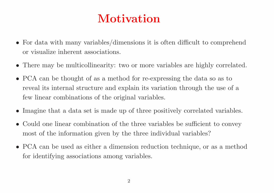
Motivation

• For data with many variables/dimensions it is often difficult to comprehend

or visualize inherent associations.

• There may be multicollinearity: two or more variables are highly correlated.

• PCA can be thought of as a method for re-expressing the data so as to

reveal its internal structure and explain its variation through the use of a

few linear combinations of the original variables.

• Imagine that a data set is made up of three positively correlated variables.

• Could one linear combination of the three variables be sufficient to convey

most of the information given by the three individual variables?

• PCA can be used as either a dimension reduction technique, or as a method

for identifying associations among variables.

2

How PCA works• The aim of PCA is to describe the variation in a set of correlated variables

X1, X2, . . . , Xm in terms of a new set of uncorrelated variables

Y1, Y2, . . . , Yp, where, hopefully, p << m, and where each Yj is a linear

combination of the X1, X2, . . . , Xm.

• The new ‘variables’, or principal components, are derived in decreasing

order of importance so that the first principal component Y1 accounts for

more variation in the original data than any other possible linear

combination of X1, X2, . . . , Xm.

• The second principal component Y2 is chosen to account for as much of the

remaining variation as possible subject to the constraint that it be

uncorrelated with Y1. And so on...

• The hope is that the first few principal components will account for a

substantial amount of the variation in the original data, and as such, can be

used as a convenient lower dimensional summary of it.

3

Sample Mean

• We have a data set consisting of n observations, each consisting of m

measurements.

• That is, we have data

x11

x12

...

x1m

,

x21

x22

...

x2m

, . . . ,

xn1

xn2

...

xnm

• The sample mean of each variable is xj =∑n

i=1xij/n.

4

Sample Covariance Matrix

• The sample covariance matrix Q is the matrix whose terms qij are defined

to be

qij =1

n− 1

n∑

k=1

(xki − xi)(xkj − xj),

for i = 1, 2, . . . ,m and j = 1, 2, . . . ,m.

• The previous results discussed for covariances of random variables also

apply for sample covariances.

• We divide by n− 1 rather than n because we have estimated the mean of

the random variables by the sample mean. If the true E[X] were known

then we would use the usual formula and divide by n. Effectively we have

lost a degree of freedom.

5

Aside: Why n− 1 and not n?

• Consider a sample of size n. It can be thought of as existing as a point in an

n dimensional space and so has n degrees of freedom in movement. Each

sample member is free to take any value it likes. If, however, you fix the

sample mean, then the sample values are constrained to have a fixed sum.

You can change n− 1 of the sample members, but the last member must

have value to ensure the sample mean is unchanged. We are interested in

the deviations from the sample mean, or in fact the product of these

deviations, and whilst we may sum over them n times, this is in truth a sum

of only n− 1 independent things.

• Of course we could use an n, but then then distributional assumptions for

the sample statistics become much more complicated to express later down

the line.

6

Linear Combinations of Data

• Let Y be a linear combination of the m variables, i.e., Y =∑m

j=1ajXi.

• Then Y = aTX.

• To determine Var(Y ) we would require Cov(X).

• Instead estimate Cov(X) through Q.

• Then Var(Y ) is estimated as aTQa.

• Similarly, if Z = bTX, then Cov(Y, Z) is estimated as aTQb = bTQa.

7

Data with 7 variables• The mean of the heptathlon data variables is,

X100m HighJump ShotPutt X200m LongJump Javelin X800m

13.9 1.78 13.8 24.6 6.10 45.0 135.5

• The sample covariance matrix of the heptathlon data is,

X100m HighJump ShotPutt X200m LongJump Javelin X800m

X100m 0.17 -0.01 -0.02 0.16 -0.09 -0.39 -0.03

HighJump -0.01 0.01 -0.03 -0.03 0.01 0.05 -0.07

ShotPutt -0.02 -0.03 1.59 -0.01 0.06 1.42 2.01

X200m 0.16 -0.03 -0.01 0.38 -0.14 -0.60 0.40

LongJump -0.09 0.01 0.06 -0.14 0.08 0.40 -0.16

Javelin -0.39 0.05 1.42 -0.60 0.40 15.80 0.47

X800m -0.03 -0.07 2.01 0.40 -0.16 0.47 24.44

• What is the mean and variance of 8× (100m time) + 4× (200m time)?

8

Eigenvalues and Eigenvectors

• The eigenvalues of a sample covariance matrix are non-negative.

• A sample covariance matrix of dimension m×m has m orthonormal

eigenvectors.

• Example: The old faithful data has sample covariance matrix

Q =

1.3 14.0

14.0 184.8

.

• The eigenvalues of Q are 185.9 and 0.244.

• The corresponding eigenvectors for these eigenvalues are

0.0755

0.9971

and

0.9971

−0.0755

.

9

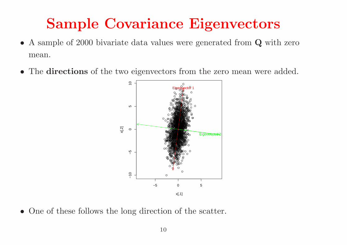
Sample Covariance Eigenvectors• A sample of 2000 bivariate data values were generated from Q with zero

mean.

• The directions of the two eigenvectors from the zero mean were added.

−5 0 5

−10

−5

05

10

x[,1]

x[,2

]

Eigenvector 1

Eigenvector 2Eigenvector 2Eigenvector 2

• One of these follows the long direction of the scatter.

10

Old Faithful Covariance Eigenvectors• Arrows in the direction of the eigenvectors were overlaid from the mean of

the actual data.

• Beware of the scaling: eigenvectors of a symmetric matrix are orthogonal!

1.5 2.0 2.5 3.0 3.5 4.0 4.5 5.0

5060

7080

90

eruptions

wai

ting

• One of these follows the long direction of scatter.

11

Heptathlon Data• More difficult to visualize!

• The eigenvalues of the sample covariance matrix are,

24.656 15.936 1.290 0.476 0.082 0.016 0.002

• The corresponding unit eigenvectors are,

[,1] [,2] [,3] [,4] [,5] [,6] [,7]

[1,] -0.002 0.025 -0.016 -0.450 0.832 -0.316 -0.075

[2,] -0.003 -0.004 0.021 0.060 0.007 -0.295 0.953

[3,] 0.091 -0.088 -0.991 0.007 0.000 0.027 0.030

[4,] 0.015 0.040 -0.013 -0.825 -0.525 -0.203 -0.006

[5,] -0.005 -0.026 -0.029 0.332 -0.180 -0.878 -0.291

[6,] 0.066 -0.992 0.094 -0.053 0.005 0.005 -0.001

[7,] 0.994 0.073 0.084 0.016 0.009 -0.006 -0.002

• Look down the columns to read off the eigenvectors.

12

Constrained Optimisation

• Consider the following problem.

• Question: Which linear combination aTX of the variables in the data has

maximum variance, subject to the constraint aTa = 1?

• We have seen that the variance of any linear combination aTX of the

variables in the data is

Var(aTX) = aTQa.

• Hence, we have the following optimisation problem.

• Problem: Find a to maximize aTQa subject to aTa = 1.

• Question: How do we solve this optimization problem?

13

Lagrange Multipliers

• Swapping notation

• Given a function f(x), the gradient of f , ∇f (the collection of partial

derivatives) indicates the direction of steepest slope. Level curves (lines

where f(x) is constant) run perpendicular to the gradient.

14

Lagrange Multipliers

• A constraint g(x) = c represents a plane that cuts through the variable

space. When the direction of the gradient of the constraint equals the

direction of the gradient of the f function, then that location constitutes a

local maxima (the actual gradients point in the same direction and differ at

most by a scalar coefficient).

15

Lagrange Multipliers

• Hence we want the location where ∇f = λ∇g.

• In other words, find x so that ∇f − λ∇g = 0.

• This gives us m+ 1 equations with m+ 1 unknowns.

16

Lagrange Multipliers

• We can use the method of Lagrange multipliers to find the maximum value

of aTQa subject to the constraint that aTa− 1 = 0.

• First, let P = aTQa− λ(aTa− 1).

• Our solution is found by computing partial derivatives∂P∂ak

, for k = 1, 2, . . . ,m, and ∂P∂λ

.

• We then seek to solve these m+1 equations when they are set to equal zero.

• Notice that ∂P∂λ

= −(aTa− 1), so solving this equation guarantees that the

constraint is satisfied.

17

Lagrange Multipliers

• Hint: Many people find it easier to switch out of matrix notation when

doing the differentiation here (but if you can do it in vector notation the

solution is much quicker).

• We can write P =∑m

i=1a2i qii +

∑mi=1

∑mj 6=i aiajqij − λ

(∑m

i=1a2i − 1

)

.

Hence,

∂P

∂ak= 2akqkk +

∑

j 6=k

ajqkj +∑

i 6=k

aiqik − 2λak

= 2akqkk + 2∑

i 6=k

aiqik − 2λak

• So,

∂P

∂ak= 0 ⇒

m∑

i=1

aiqik − λak = 0

18

Lagrange Multipliers

• We have seen that, for k = 1, . . . ,m, ∂P∂ak

= 0 implies:

(a1, a2, . . . , am)

q1k

q2k...

qmk

= λak

• This can be expressed more compactly using matrices:

(a1, a2, . . . , am)

q11 q21 · · · qm1

q12 q22 · · · qm2

......

. . ....

q1m q2m · · · qmm

= λ(a1, a2, . . . , am)

19

Lagrange Multipliers

• In matrix notation, we have

aTQ = λaT

• Taking the transpose of both sides gives,

QTa = Qa = λa

• That is, a is an eigenvector of Q. The constraint also tells us that it’s a unit

eigenvector.

• Finally, due to the maximization part of the problem, we also know it is the

eigenvector with largest eigenvalue.

Var(aTX) = aTQa = aTλa = λaTa = λ

20

Principal Components

• The first principal component of the data set is the linear combination of

the variables that has greatest variance.

• This corresponds to taking a linear combination of the variables where the

weights are as given by the eigenvector of Q with largest eigenvalue. This

eigenvalue also represents the variance of the linear combination.

• What about other principal components?

• The second principal component is the linear combination of the variables

where the weights are as given by the eigenvector of Q corresponding to the

second largest eigenvalue. Again the eigenvalue represents the variance of

this linear combination. And so on...

• All principal components are orthogonal to one another.

21

Summary• A principal components analysis constructs a set of linear combinations of

the data variables.

• Subsequent principal components have smaller and smaller variances.

• All principal components are uncorrelated with each other.

−20 −10 0 10 20 30

−1.

0−

0.5

0.0

0.5

1.0

PC1

PC

2

22