Multivariate modified Fourier series and application to boundary

value problems

Ben AdcockDAMTP, Centre for Mathematical Sciences

University of CambridgeWilberforce Rd, Cambridge CB3 0WA

United Kingdom

March 25, 2009

Abstract

In this paper we analyse the approximation-theoretic properties of modified Fourier series in Cartesianproduct domains with coefficients from full and hyperbolic cross index sets. We show that the number ofexpansion coefficients may be reduced significantly whilst retaining comparable error estimates. In doingso we extend the univariate results of Iserles, Nørsett and S. Olver. We then demonstrate that these seriescan be used in the spectral-Galerkin approximation of second order Neumann boundary value problems,which offers some advantages over standard Chebyshev or Legendre polynomial discretizations.

Introduction

Univariate modified Fourier series—eigenseries of the Laplace operator subject to homogeneous Neumannboundary conditions—were introduced in [14] as an adjustment of Fourier series. Combined with modernquadrature methods (as opposed to the Fast Fourier transform) to evaluate the coefficients, the benefit ofusing such series to approximate a non-periodic function f is a faster convergence rate (in particular theconvergence is uniform and there is no Gibbs’ phenomenon on the boundary). Moreover, the coefficientsmay be calculated adaptively in fewer operations without the restriction that the truncation parameter be ahighly composite integer. In [13] these series and quadrature methods were generalized to Cartesian productdomains.

In [11], alongside so-called polynomial subtraction (a familiar device for univariate Fourier series [15, 17]),the authors used a hyperbolic cross index set [2, 23], to accelerate convergence. Due to the method ofcalculating the coefficients, such a device can be readily exploited by modified Fourier series to produceapproximations comprising a far reduced number of terms over approximations based on Fourier series ororthogonal polynomials. Thus in higher dimensions, modified Fourier series become an increasingly attractiveoption.

The aim of this paper is twofold. In Sections 1–3 we extend the work of [11, 13] and provide convergenceanalysis for modified Fourier series in various norms using various index sets. For reasons that we makeclear, modified Fourier approximations are best analysed in so-called Sobolev spaces of dominating mixedsmoothness, [20]. Using this framework, we prove uniform convergence of such series, and provide estimatesfor the convergence rate in the L2, Hs, s ≥ 1, and uniform norms. Furthermore, we demonstrate that usingthe hyperbolic cross index set does not unduly affect the convergence rate, aside from a logarithmic factor,provided additional (mixed) smoothness assumptions are imposed where necessary.

For univariate modified Fourier series it was observed in [14] and proved in [18] that the convergence ratewas one power of N faster inside the interval than at the endpoints. We prove the same result for d-variatecubes using full and hyperbolic cross index sets. Finally, we demonstrate that the advantage of modifiedFourier series over Fourier series can be expressed as the observation that the modified Fourier basis is densenot only in L2(Ω), but also in the space H1

mix(Ω) (the first Sobolev space of dominating mixed smoothness).

1

One significant use of Fourier series is the discretization of boundary value problems with periodic bound-ary conditions. This approach offers numerous benefits, including rapid convergence and low complexity.The application of Fourier series using hyperbolic cross index sets to the numerical solution of periodicboundary value problems has been studied in [16].

Because each modified Fourier basis functions satisfies homogeneous Neumann boundary conditions,modified Fourier expansions are best suited to discretizations of non-periodic boundary value problems withthe same boundary conditions. In the second half of this paper we consider the application to linear, secondorder problems defined on d-variate cubes (see [1] for the case d = 1). Much like the Fourier spectralmethod, this technique possesses a number of beneficial properties, including reasonable conditioning andthe availability of an optimal, diagonal preconditioner. Furthermore, due to the hyperbolic cross indexset, the operational cost of this method grows only moderately with dimension. In d dimensions, we showthat the so-called modified Fourier–Galerkin approximation comprises O

(N(logN)d−1

)coefficients which

can be found in only O(N2)

operations using standard iterative techniques. In comparison, the efficientspectral-Galerkin methods of Shen, [9, 21, 22], based on Legendre and Chebyshev polynomials involveO

(Nd)

coefficients that can be found in at best O(Nd+1

)operations.

The modified Fourier basis is best suited to Neumann boundary value problems. It can be appliedto problems with other boundary conditions, however techniques for enforcing the boundary conditions areeither increasingly complicated for d ≥ 2 or lead to a loss of accuracy. For this reason, a better approach is tochoose basis functions that satisfy the boundary conditions inherently. Given, for example, Robin boundaryconditions, we use instead the basis of Laplace eigenfunctions subject to these boundary conditions. Suchbasis is very similar to the modified Fourier basis (the analysis of convergence is virtually identical), and theresulting Galerkin method possesses many similar features, including mild conditioning and low complexity.For this reason the modified Fourier–Galerkin method can be viewed as a particular example of a class ofmethods for second order boundary value problems, each with basis functions determined by the boundaryconditions. In Section 5 we present some numerical examples of discretizations of Dirichlet and Robinboundary value problems in this manner.

For the task of function approximation, modified Fourier expansions converge faster than expansionsbased on, for example, Laplace–Dirichlet eigenfunctions (which do not converge uniformly unless the functionbeing approximated also satisfies homogeneous Dirichlet boundary conditions). Hence they are the naturalchoice from such class of bases. However, for the purposes spectral discretizations (where the exact solutionautomatically satisfies the boundary conditions), each basis is immediately adapted to a particular problem.

The disadvantage of all such methods is that they converge only algebraically in terms of the truncationparameter. Standard orthogonal polynomial methods converge spectrally provided the solution is smooth.However, due to the much reduced complexity, for many test problems these methods give lower errors formoderate values of the truncation parameter. We present several such examples.

Notation: Throughout we shall write (·, ·) for the standard L2(Ω) inner product on some domain Ω. We write‖ · ‖ for the L2 norm, ‖ · ‖q for the Hq norm, q ≥ 1, and ‖ · ‖∞ for the uniform norm. N shall be a truncationparameter and IN some finite index set. We denote by f a function in L2(Ω) and u ∈ Hq(Ω) a function thatsatisfies certain derivative conditions on the boundary ∂Ω. For a multi-index α = (α1, ..., αd) ∈ Nd, Dα willcorrespond to the derivative operator

Dα =∂|α|

∂α1x1 ...∂

αdxd

= ∂α1x1...∂αdxd ,

where |α| =∑αi. If α = (r, r, ..., r), r ∈ N, we also write Dr, and, if r = 1, just D.

We define [d] to be the set of ordered tuples of length at most d with entries in 1, ..., d. For t ∈ [d] wewrite |t| for the length (number of elements) in t, so that t = (t1, ..., t|t|). If j ∈ 1, ..., d we write j ∈ t ifj = tl for some l = 1, ..., |t|. Given t ∈ [d], we define t ∈ [d] as the tuple of length d− |t| of elements not in t.

2

1 Modified Fourier series in [−1, 1]d

1.1 Definition and basic properties

The modified Fourier basis is the set of eigenfunctions of the Laplace operator subject to homogeneousNeumann boundary conditions. On the domain Ω, where Ω = (−1, 1)d, these arise from Cartesian productsof the univariate eigenfunctions

φ[0]0 (x) =

1√2, φ[0]

n (x) = cosnπx, φ[1]n (x) = sin(n− 1

2 )πx, n = 1, 2, ..., x ∈ [−1, 1].

Given multi-indices n = (n1, ..., nd) ∈ Nd and i = (i1, ..., id) ∈ 0, 1d, the d-variate eigenfunctions are

φ[i]n (x) =

d∏j=1

φ[ij ]nj (xj), x = (x1, ..., xd) ∈ [−1, 1]d, (1.1)

with corresponding eigenvalues

µ[i]n =

d∑j=1

µ[ij ]nj , where µ

[0]0 = 0, µ[0]

n = n2π2, µ[1]n = (n− 1

2 )2π2, n = 1, 2, ...

For ease of notation we shall write φ[i]n and µ

[i]n as above, with the understanding that φ[i]

n = 0 and µ[i]n = 0

if ij = 1 and nj = 0 for some j = 1, ..., d.Concerning the density of such functions, we have the following:

Lemma 1. The set φ[i]n : n ∈ Nd, i ∈ 0, 1d is an orthonormal basis of L2(−1, 1)d.

Proof. This is a standard result of spectral theory.

For a function f ∈ L2(−1, 1)d, truncation parameter N and finite index set IN ⊂ Nd, we define the truncatedmodified Fourier series of f as

FN [f ](x) =∑

i∈0,1d

∑n∈IN

f [i]n φ

[i]n (x), where f [i]

n =∫

Ω

f(x)φ[i]n (x) dx.

In [13, 14] quadrature routines are developed to evaluate these coefficients numerically. Using highly os-cillatory methods, where applicable, and so-called exotic quadrature elsewhere, any M coefficients can befound in O (M) operations. We shall not discuss such routines here. Highly oscillatory methods are greatlyadvantageous for such approximations (they facilitate the use of hyperbolic cross index sets). However, thereare a number of unresolved issues and open problems associated with their implementation, which we donot intend to address presently. We refer the reader to [13] and references therein for further detail. For theremainder of this paper we shall assume that the error in approximating the coefficients is insignificant incomparison to the error in approximating f by FN [f ].

If we define the finite dimensional space

SN = spanφ[i]n : n ∈ IN , i ∈ 0, 1d

,

then FN : L2(−1, 1)d → SN is the orthogonal projection onto SN with respect to the standard Euclideaninner product. We state, without proof, a version of Parseval’s lemma for such series:

Lemma 2 (Parseval). Suppose that f ∈ L2(−1, 1)d, ∪N≥0IN = Nd and I1 ⊂ I2 ⊂ ... ⊂ Nd. Then FN [f ] isthe best approximation to f from SN in the L2 norm, ‖f −FN [f ]‖ → 0 as N →∞ and

‖f‖2 =∑

i∈0,1d

∑n∈Nd

|f [i]n |2. (1.2)

3

Unlike its Fourier counterpart, the modified Fourier basis is not closed under differentiation. If we differentiateφ

[i]n with respect to x1, say, we obtain

∂x1φ[i]n (x) = (−1)1+i1(µ[i1]

n1)

12

ψ[1−i1]n1

(x1)d∏j=2

φ[ij ]nj (xj)

,where ψ[i]

n : i = 0, 1, n = 1, 2, ... is the set of eigenfunctions of the univariate Laplace operator subject tohomogeneous Dirichlet boundary conditions:

ψ[0]n (x) = cos(n− 1

2 )πx, ψ[1]n (x) = sinnπx, n = 1, 2, ...

In particular the Laplace–Neumann and Laplace–Dirichlet operators share eigenvalues (aside from the 0eigenvalue of the former). We conclude that ∂x1φ

[i]n (x) is proportional to an eigenfunction of the Laplace

operator on [−1, 1]d which obeys homogeneous Dirichlet boundary conditions on the subset of the boundaryΓ±1 , where

Γ±j = x ∈ [−1, 1]d : xj = ±1, j = 1, ..., d,

and homogeneous Neumann boundary conditions on Γ\(Γ+1 ∪ Γ−1 ), where Γ = ∂Ω = ∪jΓ±j . Such eigenfunc-

tions are orthogonal and dense in L2(−1, 1)d. Repeating this argument for various j we obtain:

Lemma 3 (Duality). Suppose that α = (α1, ..., αd) ∈ Nd. If we apply the operator Dα to the set of modifiedFourier eigenfunctions we obtain, up to scalar multiples, the eigenfunctions of the Laplace operator that obeyhomogeneous Dirichlet boundary conditions on the faces Γ±j where αj is odd, and homogeneous Neumannboundary conditions elsewhere. Such eigenfunctions are orthonormal and dense in L2(−1, 1)d.

This duality is essential to proving many of the convergence properties of modified Fourier series. Asmentioned, the modified Fourier basis is not only L2 dense, but also dense in various other Sobolev norms.Using this lemma, we now show this for the H1 norm:

Lemma 4. Suppose that f ∈ H1(−1, 1)d and IN is as in Parseval’s Lemma. Then ‖f − FN [f ]‖1 → 0 asN →∞. Furthermore, we have

‖f‖21 =∑

i∈0,1d

∑n∈Nd

(1 + µ[i]n )|f [i]

n |2, (1.3)

and additionally, FN [f ] is the best approximation to f from SN in the H1 norm.

Proof. It suffices to prove that ‖∂xj (f − FN [f ])‖ → 0 as N → ∞ for each j. By symmetry, it is enough toconsider the case j = 1. Now,

∂x1FN [f ](x) =∑

i∈0,1d

∑n∈INn1 6=0

f [i]n (−1)1+i1(µ[i1]

n1)

12 φ[i]

n (x),

where

φ[i]n = ψ[1−i1]

n1(x1)

d∏j=2

φ[ij ]nj (xj),

is an eigenfunction of the type introduced above. For f ∈ H1(−1, 1)d and n1 6= 0, we obtain, via Green’stheorem,

f [i]n =

∫Ω

f(x)φ[i]n (x) dx = (−1)i1(µ[i1]

n1)−

12

∫Ω

f(x)∂x1 φ[i]n (x) dx = (−1)1+i1(µ[i1]

n1)−

12

∫Ω

∂x1f(x)φ[i]n (x) dx.

Using the above relation, we see that ∂x1FN [f ](x) is precisely the orthogonal projection of ∂x1f onto

SN = spanφ[i]n : n ∈ IN , n1 6= 0, i ∈ 0, 1d.

4

By the Duality lemma, the set φ[i]n : n ∈ Nd, i ∈ 0, 1d is an orthonormal basis is of L2(−1, 1)d. In

particular, ‖∂x1(f − FN [f ])‖ → 0 as N → ∞ since ∂x1f ∈ L2(−1, 1)d. Furthermore, using a version ofParseval’s lemma for this basis we see that

‖∂x1f‖2 =∑n∈Nd

∑i∈0,1d

µ[i1]n1|f [i]n |2.

Replacing 1 by j = 2, ..., d in the above formula and summing each contribution gives (1.3). To concludethat FN [f ] is the best approximation in the H1 norm, we merely notice that FN : H1(−1, 1)d → SN is theorthogonal projection with respect to the H1 inner product.

Lemma 4 provides an equivalent characterization of the H1 norm in terms of modified Fourier coefficients.Much the same is done for Fourier series and the periodic spaces Hq(Td), for q ≥ 0. However, we cannotdo the same for modified Fourier series for q 6= 0, 1 unless we restrict to classes of functions where all theodd derivatives vanish on ∂Ω—the analogue of periodicity for modified Fourier series. We shall not fullyadopt this approach. Nonetheless, in the sequel it will be useful to consider the modified Fourier expansionof a function that satisfies a finite number of derivative conditions on the boundary. For this we have thefollowing result:

Lemma 5. Suppose that u ∈ H2k+1(−1, 1)d obeys homogeneous Neumann boundary conditions up to orderk on ∂Ω:

∂2r+1xj u

∣∣Γ±j

= 0, j = 1, ..., d, r = 0, ..., k − 1. (1.4)

Then, for r = 0, ..., 2k+1, FN [u] is the best approximation to u from SN in the Hr norm, ‖u−FN [u]‖r → 0and we have the characterization:

‖u‖2r =∑

i∈0,1d

∑n∈Nd

∑|α|≤r

d∏j=1

(µ[ij ]nj )αj

|u[i]n |2. (1.5)

Proof. This is very similar to Lemma 4. We may show (by repeated application of Green’s theorem, noticingthat the boundary integrals vanish due to (1.4)) that if u obeys the prescribed boundary conditions thenDαFN [u], |α| ≤ 2k+1, is precisely the orthogonal projection of Dαu onto the space spanned by eigenfunctionsthat satisfy homogeneous Dirichlet boundary conditions on faces Γ±j when αj is odd, and Neumann boundaryconditions elsewhere.

In the sequel we shall use a simple version of Bernstein’s inequality, which now follows immediately:

Corollary 1 (Bernstein’s Inequality). Suppose that φ ∈ SN . Then, for r ∈ N, we have

‖φ‖r ≤ maxn∈IN

(1 + µ[0]

n )r2‖φ‖. (1.6)

Proof. For i ∈ 0, 1d and n ∈ IN , µ[i]n ≤ µ[0]

n . Furthermore

(1 + µ[i]n )r =

∑|α|≤r

cα,r

d∏j=1

(µ[ij ]nj )αj (1.7)

for some constants cα,r ≥ 1. Hence, for φ ∈ SN , we obtain

‖φ‖2r ≤∑

i∈0,1d

∑n∈IN

(1 + µ[i]n )r|φ[i]

n |2 ≤ maxn∈IN

(1 + µ[0]

n )r ∑i∈0,1d

∑n∈IN

|φ[i]n |2,

and Parseval’s lemma gives the result.

An advantage of modified Fourier series is that there is no Gibbs’ phenomenon on the boundary. Indeedthe modified Fourier expansion of a sufficiently smooth function converges uniformly on [−1, 1]d. We shallnow prove this. One reason for doing so is to be able to express the error as a convergent infinite series, whichin turn will allow us to derive estimates for the pointwise and uniform rates of convergence. This shall requireparticular choices of the index set IN , which we defer to the sequel. However, uniform convergence may beproved independently of the choice of index set. To do so we must consider Sobolev spaces of dominatingmixed smoothness.

5

1.2 Sobolev spaces of dominating mixed smoothness

Sobolev spaces of dominating mixed smoothness are the standard setting whenever a hyperbolic cross indexset is employed, [3, 20, 23]. In the particular case of modified Fourier series, even for full index sets, suchspaces provide a suitable framework for analysis.

It turns out that the modified Fourier basis is not just dense in the space H1(−1, 1)d, but also in the firstSobolev space of dominating mixed smoothness, which we denote H1

mix(−1, 1)d. This fact ensures uniformconvergence of FN [f ] to f which we shall prove in the next section.

Subsequently we shall also see that the corresponding norms are precisely those required to bound themodified Fourier coefficients f [i]

n in inverse powers of n1...nd, which leads to quasi-optimal error estimatesand justifies the use of a hyperbolic cross index set.

For k ∈ N we define the kth Sobolev space of dominating mixed smoothness by

Hkmix(−1, 1)d = f : Dαf ∈ L2(−1, 1)d, ∀ α : |α|∞ ≤ k, (1.8)

where |α|∞ = maxαi, with norm‖f‖2k,mix =

∑|α|∞≤k

‖Dαf‖2. (1.9)

This space is also commonly denoted by S(k,...,k)2 H(−1, 1)d in literature, [20, 23].

In an identical manner to Lemma 5, we may characterize the H1mix norm in terms of modified Fourier

coefficients. We merely notice (recalling the proof of Lemma 4) that DαFN [f ] is the orthogonal projectiononto some suitable finite dimensional space not just for |α| ≤ 1, but also for |α|∞ ≤ 1. This yields:

Lemma 6. Suppose that f ∈ H1mix(−1, 1)d. Then, FN [f ] is the best approximation to f from SN in the H1

mix

norm, ‖f −FN [f ]‖1,mix → 0 and we have the characterization:

‖f‖21,mix =∑

i∈0,1d

∑n∈Nd

∑|α|∞≤1

d∏j=1

(µ[ij ]nj )αj

|f [i]n |2. (1.10)

Furthermore, suppose that u ∈ H2k+1mix (−1, 1)d satisfies the first k derivative conditions (1.4). Then, for

r = 0, 1, ..., 2k + 1, FN [u] is the best approximation to u in the Hrmix norm, ‖u−FN [u]‖r,mix → 0 and

‖u‖2r,mix =∑

i∈0,1d

∑n∈Nd

∑|α|∞≤r

d∏j=1

(µ[ij ]nj )αj

|u[i]n |2. (1.11)

1.3 Uniform convergence

We commence with the following lemma:

Lemma 7. Suppose that f ∈ H1mix(−1, 1)d. Then, f ∈ C[−1, 1]d and there is a constant c independent of f

such that‖f‖∞ ≤ c‖f‖1,mix. (1.12)

To prove this we need the following lemma:

Lemma 8. Suppose that f ∈ C∞[−1, 1]d. Then

f(x) =∑t∈[d]

∫ xt1

−1

...

∫ xt|t|

−1

Dtf(xt,−1) dxt1 ...dxt|t| + f(−1, ...,−1), x ∈ [−1, 1]d. (1.13)

where [d] is the set of ordered tuples of length at most d with entries in 1, ..., d, Dt = ∂xt1 ...∂xt|t| for

t = (t1, ..., t|t|) ∈ [d] and (xt,−1) ∈ Rd has jth entry xj if j ∈ t and −1 otherwise.

6

Proof. We use induction on d. For d = 1 we have f(x) =∫ x−1f ′(x) dx + f(−1), so the result holds. Now

assume that (1.13) holds for d− 1. Then

f(x) =∫ xd

−1

∂xdf(x) dxd + f(x1, ..., xd−1,−1)

=∑

t∈[d−1]

∫ xt1

−1

...

∫ xt|t|

−1

∫ xd

−1

∂xdDtf((xt, xd),−1) dxt1 ...dxt|t|dxd

+∑

t∈[d−1]

∫ xt1

−1

...

∫ xt|t|

−1

Dtf(xt,−1) dxt1 ...dxt|t| +∫ xd

−1

∂xdf(xd,−1) dxd + f(−1, ...,−1).

Since the set [d] is comprised of elements t, (t, d) = (t1, ..., t|t|, d), (d), where t ∈ [d − 1], this expressionreduces to (1.13). Hence the proof is complete.

Proof of Lemma 7. We first prove the result for f ∈ C∞[−1, 1]d. We note that

f(xt,−1) = 2d−|t|∫ 1

−1

...

∫ 1

−1

Dt

f(x)∏j /∈t

(xj − 1)

dxt1 ...dxtd−|t| , ∀t ∈ [d],

where t ∈ [d] is the tuple of length d− |t| of elements not in t. Hence, using Lemma 8, we have

f(x) =∑t∈[d]

∫ 1

−1

...

∫ 1

−1

∫ xt1

−1

...

∫ xt|t|

−1

D

f(x)∏j /∈t

(xj − 1)

dxt1 ...dxt|t|dxt1 ...dxtd−|t|

+∫ 1

−1

...

∫ 1

−1

D

f(x)d∏j=1

(xj − 1)

dx1...dxd.

Each integrand involves terms of the form Dαf for some |α|∞ ≤ 1. Hence, using the Cauchy–Schwarzinequality and replacing suitable upper limits of integration by 1, we obtain (1.12) for f ∈ C∞[−1, 1]d.

We now proceed in the standard manner. If f ∈ H1mix(−1, 1)d then f is the limit in H1

mix(−1, 1)d of asequence of functions belonging to C∞[−1, 1]d. Since (1.12) holds for f ∈ C∞[−1, 1]d this sequence convergesuniformly on [−1, 1]d to f ∈ C[−1, 1]d. Since f = f a.e. the result follows.

Theorem 2. Suppose that f ∈ H1mix(−1, 1)d and IN satisfies the conditions of Parseval’s lemma. Then,

FN [f ] converges pointwise to f for all x ∈ [−1, 1]d. Moreover, the convergence is uniform.

Proof. Replacing f by f −FN [f ] in (1.12) and applying Lemma 6 gives the result.

Prior to considering various different choices of index set and the corresponding error estimates for modifiedFourier series, we need to develop bounds for the modified Fourier coefficients:

1.4 Bounds for modified Fourier coefficients

We commence with the following lemma:

Lemma 9. Suppose that f ∈ H1mix(−1, 1)d and n ∈ Nd+ = (N\0)d. Then

f [i]n = (−1)d+|i|

d∏j=1

µ[ij ]nj

− 12 ∫

Ω

Df(x)ψ[1−i]n (x) dx, (1.14)

where 1− i is the multi-index (1− i1, ..., 1− id).

Proof. This is obtained by repeated application of Green’s theorem.

7

To obtain robust bounds for the coefficients f [i]n we need to apply Green’s theorem to the right hand

side of (1.14). However, in this case the boundary integrals are non-vanishing, so we need some additionalnotation. Given a tuple t ∈ [d] and x = (x1, ..., xd) ∈ Rd we define xt = (xt1 , ..., xt|t|) ∈ R|t|. Further, for

i ∈ 0, 1 and j = 1, ..., d we define the operator 4[i]j : H1

mix(−1, 1)d → H1mix(−1, 1)d−1 by

4[i]j [g](x1, ..., xj−1, xj+1, ..., xd) = g(x1, ..., xj−1, 1, xj+1, ..., xd) + (−1)i+1g(x1, ..., xj−1,−1, xj+1, ..., xd).

Given t = (t1, ..., t|t|) ∈ [d] and i ∈ 0, 1|t| we define 4[i]t : H1

mix(−1, 1)d → H1mix(−1, 1)d−|t| by

4[i]t [g] = 4[i1]

t1

[4[i2]t2

[...[4[i|t|]t|t|

[g]]]]

.

Note that the operators 4[it1 ]t1 , ...,4

[it|t| ]

t|t|commute with each other and with partial differentiation in the

independent variables. Further if g is a function of x ∈ [−1, 1]d then 4[i]t [g] is a function of xt.

Finally, given t ∈ [d], i ∈ 0, 1d and n ∈ Nd−|t| we define Θ[i]t,n : H1

mix(−1, 1)d → R by

Θ[i]t,n[g] = 4[it]

t [Dtg][it]

n ,

where Dt = ∂xt1 ...∂xt|t|. With this in hand we may now deduce the key result of this section:

Lemma 10. Suppose that g ∈ H1mix(−1, 1)d and n ∈ Nd+. Then

∫Ω

g(x)ψ[1−i]n (x) dx = (−1)|i|

d∏j=1

µ[ij ]nj

− 12∑t∈[d]

(−1)|nt|+|it|+|t|Θ[i]t,nt

[g] + Dg[i]

n

.

Proof. It suffices to prove this result for g ∈ C∞[−1, 1]d. To cover the general case we use density, linearityand the bound ∣∣Θ[i]

t,n[f ]∣∣ ≤ c‖f‖1,mix, ∀f ∈ H1

mix(−1, 1)d,

for some constant c > 0 (see Lemma 12). We proceed by induction on d. For d = 1 trivial integration byparts verifies the result. Indeed, we have∫ 1

−1

g(x)ψ[1−i]n (x) dx = (−1)i

(µ[i]n

)− 12(

(−1)n+i+14[i]1 [g] + Dg

[i]

n

).

Suppose that the result is true for d− 1. Then, for g ∈ C∞[−1, 1]d we have∫Ω

g(x)ψ[1−i]n (x) dx =

∫(−1,1)d−1

hnd(x′)ψ[1−i′]n′ (x′) dx′

where x′ = (x1, ..., xd−1), i′ = (i1, ..., id−1) and n′ = (n1, ..., nd−1) are the first d − 1 entries of x, i and nrespectively, and

hnd(x′) =∫ 1

−1

g(x)ψ[1−id]nd

(xd) dxd.

By induction:

∫Ω

g(x)ψ[1−i]n (x) dx = (−1)|i

′|

d−1∏j=1

µ[i′j ]

n′j

− 12 ∑t′∈[d−1]

(−1)|nt′ |+|it′ |+jΘ[i′]t′,n′

t′[hnd ] + Dhnd

[i′]

n′

. (1.15)

Using the formula for d = 1 we may write

hnd(x′) = (−1)id(µ[id]nd

)− 12(

(−1)nd+id+14[id]d [g](x′) + ∂xdg

[id]

nd

).

8

Now we consider terms of (1.15) separately. We have

Θ[i′]t′,n′

t′[4[id]

d [Dt′g]] = Θ[i]t,nt

[g],

where t = (t′, d) ∈ [d]. Also

Θ[i′]t′,n′

t′

[∂xdg

[id]

nd

]= Θ[i]

t,nt[g],

where, in this case, t = t′ ∈ [d]. For the second term of (1.15) we have

Dhnd[i′]

n′ = (−1)id(µ[id]nd

)− 12

((−1)nd+id+1 4[id]

d [Ddg][i′]

n′+ Dg

[i]

n

)

= (−1)id(µ[id]nd

)− 12(

(−1)nd+id+1Θ[i]d,n[g] + Dg

[i]

n

),

where d = (1, ..., d− 1) ∈ [d]. Combining these results, we obtain

g[1−i]n = (−1)|i|

d∏j=1

µ[ij ]nj

− 12 ∑

t′∈[d−1]

(−1)|nt′ |+|it′ |+|t′|(

(−1)nd+id+1Θ[i]t,nt

[g] + Θ[i]t′,nt′

[g])

+ (−1)nd+id+1Θ[i]d,n[g] + Dg

[i]

n

,

where t = (t′, d). Now, the set [d] contains precisely elements (t′, d), t′, and (d) where t′ ∈ [d− 1]. The firstthree terms in the above sum correspond to each of these. Furthermore

if t = (t′, d), then |nt| = |nt′ |+ nd, |it| = |it′ |+ id, |t| = |t′|+ 1,if t = t′, then |nt| = |nt′ |, |it| = |it′ |, |t| = |t′|,if t = (d), then |nt| = nd, |it| = id, |t| = 1.

With this in hand, we obtain the result.

Corollary 3. Suppose that f ∈ H2mix(−1, 1)d and n ∈ Nd+. Then

f [i]n = (−1)d

d∏j=1

µ[ij ]nj

−1∑t∈[d]

(−1)|nt|+|it|+|t|Θ[i]t,nt

[Df ] + D2f[i]

n

.

Iterating this formula immediately yields the following:

Theorem 4. Suppose that f ∈ H2kmix(−1, 1)d and n ∈ Nd+. Then

f [i]n =

k−1∑r=0

(−1)dd∏j=1

µ[ij ]nj

−(r+1)∑t∈[d]

(−1)|nt|+|it|+|t|Θ[i]t,nt

[D2r+1f ]

+ (−1)kd

d∏j=1

µ[ij ]nj

−k D2kf[i]

n .

If f obeys the first k derivative conditions then the first k terms vanish.

Proof. To obtain the formula we use Corollary 3. Now suppose that f obeys the prescribed derivativeconditions. It follows that D2r+1f , r = 0, ..., k− 1, vanishes on the boundary. Since each of the first k termsinvolves at least one evaluation of D2r+1f on the boundary, we deduce the result.

Thus far we have assumed that n ∈ Nd+. Now suppose that nt1 = ...nt|t| = 0 for some t ∈ [d]. Then

f[i]n = ft

[it]

ntwhere ft is the function defined by

ft(xt) =∫ 1

−1

...

∫ 1

−1

f(x) dxt1 ...dxt|t| .

9

Hence Theorem 4 may be used for ft and in turn for f [i]n when n ∈ Nd.

As examples of Theorem 4, consider the cases d = 1, 2. For d = 1 we have

f [i]n =

k−1∑r=0

(−1)n+i

(µ[i]n )r+1

4[i][f (2r+1)] +(−1)k

(µ[i]n )k

f (2k)[i]

n , n ∈ N, i ∈ 0, 1,

and for d = 2 with k = 1 the corresponding result is

f [i]n =

1

µ[i1]n1 µ

[i2]n2

(−1)n1+n2+i1+i24[i][∂x1∂x2f ] + (−1)n1+i1+1 4[i1][∂x1∂

2x2f ]

[i2]

n2

+ (−1)n2+i2+1 4[i2][∂2x1∂x2f ]

[i1]

n1+ ∂2

x1∂2x2f

[i]

n

, n ∈ N2

+, i ∈ 0, 12,

f[i1,0]n1,0

=1

µ[i1]n1

(−1)n1+i1 4[i1][∂x1f ]

[0]

0 − ∂2x1f

[i1,0]

n1,0

, n1 ∈ N+, i1 ∈ 0, 1,

f[0,i2]0,n2

=1

µ[i2]n2

(−1)n2+i2 4[i2][∂x2f ]

[0]

0 − ∂2x2f

[0,i2]

0,n2

, n2 ∈ N+, i2 ∈ 0, 1.

We now wish to derive bounds for the coefficients f [i]n . To do so it is useful to consider the following Sobolev

spaces:Gkmix(−1, 1)d =

f : Dαf ∈ L1(−1, 1)d, ∀ α : |α|∞ ≤ k, k ∈ N,

with norm‖|f |‖k,mix =

∑|α|∞≤k

‖Dαf‖L1(−1,1)d .

Regarding such spaces, we have the following result which we shall use in the sequel:

Lemma 11. Suppose that f ∈ Hkmix(−1, 1)d, k ∈ N. Then f ∈ Gkmix(−1, 1)d and ‖|f |‖k,mix ≤ (2k+2)

d2 ‖f‖k,mix.

Proof. The first result follows immediately since L2(−1, 1)d ⊂ L1(−1, 1)d. For the second, we use theCauchy–Schwarz inequality to obtain

‖|f |‖k,mix ≤ 2d2

∑|α|∞≤k

‖Dαf‖ ≤ 2d2

∑|α|∞≤k

1

12

‖f‖k,mix.

Since there are (k + 1)d choices of α ∈ Nd with |α|∞ ≤ k we obtain the result.

To derive coefficient bounds we first need the following lemma:

Lemma 12. Suppose that f ∈ H1mix(−1, 1)d, i ∈ 0, 1|t|, t ∈ [d] and n ∈ Nd−|t|. Then∣∣Θ[i]

t,n[f ]∣∣ ≤ ‖|f |‖1,mix

Proof. For i ∈ 0, 1 and j = 1, ..., d we have

4[i]j [f ] =

∫ 1

−1

∂xj(f(x)xij

)dxj .

This implies that

4[i]t [f ] =

∫ 1

−1

...

∫ 1

−1

Dt

f(x)∏j∈t

xijj

dxt1 ...dxt|t| , t ∈ [d], i ∈ 0, 1d.

10

Hence

Θ[i]t,n[f ] =

∫Ω

D

f(x)∏j∈t

xijj

∏j /∈t

φ[ij ]nj (xj) dx.

We deduce that ∣∣Θ[i]t,n[f ]

∣∣ ≤ ∫Ω

∣∣∣∣∣Df(x)

∏j∈t

xijj

∣∣∣∣∣ dx ≤ ‖|f |‖1,mix,

Note that the final inequality follows since the integral is a sum over derivatives Dαg with |α|∞ ≤ 1 eachmultiplied by xβ1

1 ...xβdd for some suitable multi-index |β|∞ ≤ 1.

Using this lemma we deduce the following:

Theorem 5. Suppose that f ∈ H2k+2mix (−1, 1)d obeys the first k derivative conditions. Then

∣∣f [i]n

∣∣ ≤ 2χ(n)

∏j:nj>0

µ[ij ]nj

−(k+1)

‖|f |‖2k+2,mix, n ∈ Nd,

where χ(n), the grade of n, is the number of non-zero entries.

Proof. Suppose first that n ∈ Nd+. Then, since f obeys the first k derivative conditions,

|f [i]n | ≤

d∏j=1

µ[ij ]nj

−(k+1) d∑l=1

∑|t|=l

∣∣Θ[i]t,n[D2k+1f ]

∣∣+∣∣D2k+2f

[i]

n

∣∣≤

d∏j=1

µ[ij ]nj

−(k+1)1 +d∑l=1

∑|t|=l

1

‖|f |‖2k+2,mix ≤ 2d

d∏j=1

µ[ij ]nj

−(k+1)

‖|f |‖2k+2,mix,

since there are(dl

)choices of t ∈ [d] with |t| = l. Now suppose that nj = 0 for j ∈ t ,where t ∈ [d]. Then,

using the previous result,

|f [i]n | = |ft

[i]

n | ≤ 2χ(n)

∏j:nj>0

µ[ij ]nj

−(k+1)

‖|ft|‖2k+2,mix.

Moreover,

‖|ft|‖2k+2,mix =∑

|α|∞≤2k+2

α∈Nχ(n)

∫(−1,1)χ(n)

∣∣Dαft(x)∣∣ dx ≤ ∑

|α|∞≤2k+2

α∈Nχ(n)

∫(−1,1)d

∣∣Dαf(x)∣∣ dx ≤ ‖|f |‖2k+2,mix.

Hence we obtain the result.

Using Lemma 11 we may also derive a bound for f [i]n in terms of ‖f‖2k+2,mix:

Corollary 6. Suppose that f ∈ H2k+2mix (−1, 1)d obeys the first k derivative conditions. Then

∣∣f [i]n

∣∣ ≤ 2χ(n)+ d2 (2k + 3)

χ(n)2

∏j:nj>0

µ[ij ]nj

−(k+1)

‖f‖2k+2,mix, n ∈ Nd.

11

Proof. If χ(n) = d the result follows immediately from Theorem 5 and Lemma 11. Now suppose thatχ(n) < d. We then have

|f [i]n | ≤ 2χ(n)

∏j:nj>0

µ[ij ]nj

−(k+1)

‖|ft|‖2k+2,mix.

Furthermore, ‖|ft|‖2k+2,mix ≤ (4k + 6)χ(n)

2 ‖ft‖2k+2,mix and

‖Dαft‖ ≤ 2d2−

χ(n)2 ‖Dαf‖, α ∈ Nχ(n).

Combining these observations we obtain ‖|ft|‖2k+2,mix ≤ 2d2 (2k+3)

χ(n)2 ‖f‖2k+2,mix, completing the proof.

For the results of subsequent sections the following corollary is in fact more useful:

Corollary 7 (Coefficient bounds). Suppose that f ∈ H2k+2mix (−1, 1)d obeys the first k derivative conditions.

Then ∣∣f [i]n

∣∣ ≤ 2χ(n)+ d2 (2k + 3)

χ(n)2 (2|i|π−χ(n))2(k+1)(n1...nd)−2(k+1)‖f‖2k+2,mix, n ∈ Nd,

where m = maxm, 1 for m ∈ N.

Proof. For n ∈ N+ and i ∈ 0, 1 it is easily shown that µ[i]n ≥ (2|i|π−1)−2n2. The result now follows

immediately from Corollary 6.

These are bounds precisely what is needed to provide quasi-optimal estimates for the error f − FN [f ] invarious norms using various index sets, as we shall see in the next two sections.

2 Full index sets

The results of the previous sections do not make any assumptions regarding the index set IN aside from thestipulations that IN be finite, ∪NIN = Nd and I1 ⊂ I2 ⊂ .... ⊂ Nd. The size of IN determines the cost ofconstructing the approximation FN [f ]: using numerical quadrature, the number of operations to evaluatethe coefficients is O (|IN |). Standard intuition leads to the full index set

IN =n ∈ Nd : max

j=1,...,dnj ≤ N

, (2.1)

which is just the hypercube of length N + 1 in Nd. Indeed, the prevalence of this index set in spectraldiscretizations is due to the fact that the method of choice for evaluating Fourier or Chebyshev coefficients,namely the FFT, computes all the coefficients in IN in a non-adaptive way. However, |IN | = O

(Nd)

andthis figure grows exponentially with dimension. To alleviate this problem we employ a hyperbolic cross indexset in the sequel. Nonetheless, for the purposes of comparison, in the remainder of this section we considerthe approximation properties of modified Fourier series based on (2.1). In the univariate case, this has beenthoroughly dealt with in [1], [14] and [18]. We now extend these results to the multivariate setting.

2.1 Pointwise and uniform convergence rate

Our first theorem generalizes the univariate result of S. Olver, [18], to d-variate cubes:

Theorem 8. Suppose that f ∈ H3mix(−1, 1)d and IN is the full index set (2.1). Then the error f(x)−FN [f ](x)

is O(N−2

)uniformly in any compact subset of (−1, 1)d.

Proof. We can always rewrite a function f as a linear combination of terms of the form f(±x1, x2, ..., xd),f(x1,±x2, x3, ..., xd), and so on. This allows us to express f as a sum of functions which only have non-zeromodified Fourier coefficients for only one specific value of i. For example, if d = 1, we have

f(x) =12

[f(x) + f(−x)] +12

[f(x)− f(−x)] ,

12

where 12 [f(x) + f(−x)] and 1

2 [f(x)− f(−x)] have only non-zero modified Fourier coefficients for i = 0 andi = 1 respectively. Hence it suffices to consider a function f with non-zero modified Fourier coefficients forjust one specific value of i. Since such cases are similar, we shall take i = 0.

We use induction on d. The case d = 1 has been dealt with in [18], so we shall not repeat it here. Supposethat the result is true for d − 1. Then, to simplify matters we first reformulate f so that fn (dropping the[i] superscript) is nonzero only when every component of n is positive. This may be achieved as follows. Weset f0(x) = f(x) and then, given f1, ..., fr, we define fr+1 for r ≤ d− 1 by

fr+1(x) = fr(x)− 2−(d−r)∑t∈[d]|t|=d−r

∫Ωt

fr(x) dx,

where Ωt is the (d − r)-dimensional subset of Ω spanned by xt1 , ..., xtd−r . The new function f = fd hasnonzero modified Fourier coefficients only when each component of n is nonzero. To see this we first assertthe following: ∫

Ωt

fr+1(x) dx = 0, whenever t ∈ [d], |t| ≥ d− r.

In particular ∫Ωt

f(x) dx = 0, t ∈ [d].

We prove this by induction. Since

f1(x) = f(x)− 2−d∫

Ω

f(x) dx,

the result is true for r = 0. Now suppose that the result holds for r − 1. If we integrate fr+1 over any Ωtwith |t| ≥ d − r the first term cancels with the term in the sum corresponding to t. All other terms in thesum are zero since they are integrals of fr over subsets of the boundary of dimension at least d− r+ 1. Thuswe obtain the result.

From this, it is simple to show that f satisfies the desired property. Note that f may be expressed asf + g where g is a linear combination of functions of d− 1 variables. Thus, to prove the theorem it sufficesto consider only f , which we now rewrite as f , and use induction on g to obtain the result. Finally, we notethat f and g have the same smoothness properties as f .

Dropping the [i] superscript and using Corollary 3 gives

fn = (−1)d

d∏j=1

(njπ)−2

∑t∈[d]

(−1)|nt|+|t|Θt,nt [Df ] + D2fn

= (−1)d

d∏j=1

(njπ)−2

(−1)|n|cf +∑|t|<d

(−1)|nt|+|t|Θt,nt [Df ] + D2fn

, (2.2)

where is a constant depending on f only. Using Theorem 2 we may express the error as

f(x)−FN [f ](x) =∑t∈[d]

N∑nj=1j /∈t

∑nj>Nj∈t

fnφn(x). (2.3)

Suppose that we define the univariate functions

Φ(N, x) = g(x)−FN [g](x) =∑n>N

(−1)n

(nπ)2cosnπx, Ψ(N, x) = FN [g](x) =

N∑n=1

(−1)n

(nπ)2cosnπx,

13

where g(x) = 14x

2 − 112 . Then the contribution of first term of (2.2) to (2.3) is

cf∑n/∈IN

(−1)|n|d∏j=1

(njπ)−2 cosnjπxj = cf∑t∈[d]

∏j /∈t

Ψ(N, xj)∏j∈t

Φ(N, xj). (2.4)

We have Φ(N, x) = O(N−2

)uniformly for x in closed subsets of (−1, 1), [18]. Trivially Ψ(N, x) is uniformly

bounded in N and x. Hence (2.4) is O(N−2

)uniformly in any compact subset of (−1, 1)d.

We deal with the other terms in the expansion of fn in a similar manner. Consider a term of the form d∏j=1

(njπ)−2

(−1)|ns|+|s|Θs,ns [Df ], s ∈ [d], |s| < d.

The contribution of this term to the error is

∑t∈[d]

( N∑nj=1j /∈t

(njπ)−2)( ∑

nj>Nj∈t

(njπ)−2)

(−1)|ns|+|s|Θs,ns [Df ]. (2.5)

Using the same method as in the proof of Lemma 12 it can be shown that∣∣Θs,ns [Df ]∣∣ =

∣∣ 4s[D1Dsf ]n∣∣ ≤ c‖f‖3,mix

∏j /∈s

n−1j .

Suppose that x is in a compact subset of (−1, 1)d. We consider the terms of (2.5) separately for each t ∈ [d]. Ift and s do not have any common entry then there must be an infinite sum of the form

∑n>N n

−3 = O(N−2

).

On the other hand, if t and s have at least one common entry j then we may factor out a term of the formΦ(N, xj), which is O

(N−2

), giving the result.

To bound the contribution of the final term of (2.2) we merely note that D2fn = O(n−1

1 ...n−1d

).

This theorem excludes subsets of the boundary from the error estimate. Dealing with such regions ismuch easier, we merely use a bound for the uniform error. For such a bound, we need lower smoothness:

Lemma 13. Suppose that f ∈ H2mix(−1, 1)d and IN is the full index set (2.1). Then

‖f −FN [f ]‖∞ ≤ c0‖f‖2,mixN−1 + lower order terms,

where ζ(·) is the zeta function and

c0 =d5d21+ d

2

π2

√3[1 + 2

√3π−2ζ(2)

]d−1

.

Proof. We have

‖f −FN [f ]‖∞ ≤∑

i∈0,1d

∑n/∈IN

|f [i]n | ≤ ‖f‖2,mix

∑i∈0,1d

22|i|∑t∈[d]

N∑nj=1j /∈t

∑nj>Nj∈t

2χ(n)+ d2 3

χ(n)2 π−2χ(n)(n1...nd)−2.

The largest contribution occurs when |t| = 1. Since there are d such possible t ∈ [d] we obtain

‖f −FN [f ]‖∞ ≤ d5d21+ d2√

3π−2‖f‖2,mix

(1 + 2

√3π−2

N∑n=1

n−2

)d−1 ∑n>N

n−2 + lower order terms.

For r > 1,∑Nn=1 n

−r−1 = ζ(r + 1) +O (N−r) and∑n>N n

−r−1 = r−1N−r +O(N−r−1

), hence we obtain

the result.

14

For the purposes of spectral-Galerkin methods based on modified Fourier series, Theorem 8 is somewhatsuperfluous: the Galerkin approximation does not normally possess a faster convergence rate inside theinterval. In that case, Lemma 13 is better suited.

When a function u satisfies the first k derivative conditions, these rates of convergence increase by afactor of N2k. By identical arguments we obtain:

Theorem 9. Suppose that u ∈ H2k+2mix (−1, 1)d satisfies the first k derivative conditions and IN is the full

index set (2.1). Then‖u−FN [u]‖∞ ≤ ck‖u‖2k+2,mixN

−2k−1,

where

ck =d(1 + 4k+1)d21+ d

2

(2k + 1)π2(k+1)

√2k + 3

[1 + 2

√2k + 3π−2(k+1)ζ(2k + 2)

]d−1

.

Moreover, if u ∈ H2k+3mix (−1, 1)d, then the error u(x) − FN [u](x) is O

(N−2k−2

)uniformly in any compact

subset of (−1, 1)d.

2.2 Estimates in other norms

Concerning the error in the Hs norm, we have:

Lemma 14. Suppose that u ∈ H2k+1(−1, 1)d satisfies the first k derivative conditions and IN is the fullindex set (2.1). Then

‖u−FN [u]‖s ≤ cr,sNs−r‖u‖r, r = s, ..., 2k + 1, s = 0, ..., 2k + 1, (2.6)

for some positive constant cr,s independent of u and N .

Proof. For n /∈ IN , µ[i]n ≥ (Nπ)2. Using this, Lemma 5 and (1.7) we have

‖u−FN [u]‖2s ≤∑

i∈0,1d

∑n/∈IN

(1 + µ[i]n )s|u[i]

n |2 ≤ (Nπ)2(s−r)∑

i∈0,1d

∑n/∈IN

(1 + µ[i]n )r|u[i]

n |2

≤ cr,sN2(s−r)∑

i∈0,1d

∑n∈Nd

∑|α|≤r

d∏j=1

(µ[ij ]nj )αj |u[i]

n |2 = cr,sN2(s−r)‖u−FN [u]‖2r,

as required.

The conclusion of Lemma 14 may lead to the assertion that, for smooth u satisfying the first k oddderivative conditions, the H1 error, for example, is O(N−2k). However, this is not the case: the H1 error isO(N−2k− 1

2 ), which we shall now prove. To show this, instead of using the above method of proof, we utilizethe coefficient bounds of Section 1.4.

Lemma 15. Suppose that u ∈ H2k+2mix (−1, 1)d satisfies the first k derivative conditions and IN is the full

index set (2.1). Then

‖u−FN [u]‖s ≤ csNs−2k− 32 ‖u‖2k+2,mix + lower order terms, s = 0, ..., 2k + 1, (2.7)

where

cs =

√d(1 + 16k+1

) d−12 21+ d

2

π2(k+1)−s(4k + 3− 2s)

√2k + 3

[1 + 4(2k + 3)π−4(k+1)ζ(4k + 4)

] d−12.

Proof. Using Lemma 5 we have

‖u−FN [u]‖2s =∑

i∈0,1d

∑|α|≤s

∑t∈[d]

N∑nj=1j /∈t

∑nj>Nj∈t

|u[i]n |2

d∏j=1

(µ[ij ]nj )αj .

15

Since u[i]n = O

((n1...nd)−2k−2

)the largest contribution occurs when |t| = 1 and αj = s if j ∈ t and 0

otherwise. Hence, as in the proof of Lemma 13, we obtain

‖u−FN [u]‖2s ≤ d∑

i∈0,1d

N∑nj=1

j=1,...,d−1

∑nd>N

|u[i]n |2(µ[id]

nd)s + lower order terms.

After an application of the Coefficient bounds corollary and using arguments similar to those given in Lemma13 we obtain the result.

3 Hyperbolic cross index sets

A hyperbolic cross index set is obtained by including only those terms in the expansion∑i∈0,1d

∑n∈Nd

f [i]n φ

[i]n (x),

whose absolute value in some norm is greater than some tolerance ε. To do so, we need some bound for thecoefficients f [i]

n and the functions φ[i]n . Given a norm ‖| · |‖, we use the coefficient bounds of Section 1.4:

‖|f [i]n φ

[i]n |‖ ≤ c‖f‖2,mix‖|φ[i]

n ‖|(n1...nd)−2.

We shall consider the index set that originates from the L2 and uniform norms. In this case ‖φ[i]n ‖∞ = ‖φ[i]

n ‖ =1, and ‖|f [i]

n φ[i]n |‖ ≤ c‖f‖2,mix(n1...nd)−2. The tolerance ε is precisely this upper bound with n = (N, 1, ...1),

in other words ε = c‖f‖2,mixN−2. This yields the hyperbolic cross, [2, 23], index set

IN = n ∈ Nd : n1...nd ≤ N. (3.1)

We devote the remainder of this section to showing the benefit of this index set. There are two aspectsto this: the reduced cost in forming the approximation—in other words, the reduced size of the hyperboliccross index set—and the retention of the similar error estimates in comparison to approximations based onthe full index set (2.1). We commence with the former:

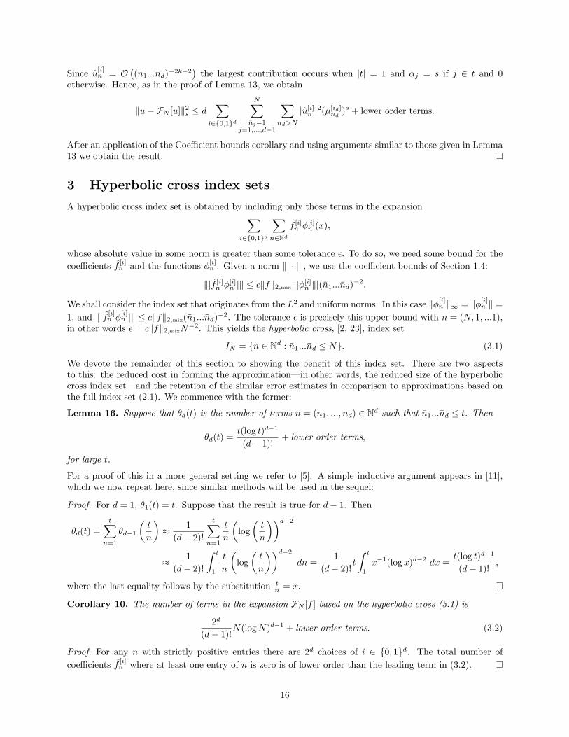
Lemma 16. Suppose that θd(t) is the number of terms n = (n1, ..., nd) ∈ Nd such that n1...nd ≤ t. Then

θd(t) =t(log t)d−1

(d− 1)!+ lower order terms,

for large t.

For a proof of this in a more general setting we refer to [5]. A simple inductive argument appears in [11],which we now repeat here, since similar methods will be used in the sequel:

Proof. For d = 1, θ1(t) = t. Suppose that the result is true for d− 1. Then

θd(t) =t∑

n=1

θd−1

(t

n

)≈ 1

(d− 2)!

t∑n=1

t

n

(log(t

n

))d−2

≈ 1(d− 2)!

∫ t

1

t

n

(log(t

n

))d−2

dn =1

(d− 2)!t

∫ t

1

x−1(log x)d−2 dx =t(log t)d−1

(d− 1)!,

where the last equality follows by the substitution tn = x.

Corollary 10. The number of terms in the expansion FN [f ] based on the hyperbolic cross (3.1) is

2d

(d− 1)!N(logN)d−1 + lower order terms. (3.2)

Proof. For any n with strictly positive entries there are 2d choices of i ∈ 0, 1d. The total number ofcoefficients f [i]

n where at least one entry of n is zero is of lower order than the leading term in (3.2).

16

3.1 Convergence rate in various norms

We now assess the rate of convergence of the approximation FN [u] based on the hyperbolic cross (3.1) invarious norms:

Lemma 17. Suppose that u ∈ H2k+1(−1, 1)d satisfies the first k derivative conditions (1.4) and IN is thehyperbolic cross index set (3.1). Then, for some positive constant cr,s independent of u and N ,

‖u−FN [u]‖s ≤ cr,sNs−rd ‖u‖r, r = s, ..., 2k + 1, s = 0, ..., 2k + 1. (3.3)

If, additionally, u ∈ H2k+1mix (−1, 1)d, then

‖u−FN [u]‖s ≤ cr,sNs−r‖u‖r,mix, r = s, ..., 2k + 1, s = 0, ..., 2k + 1. (3.4)

Proof. Due to Lemma 5 and (1.7) we may write

‖u−FN [u]‖2s ≤∑

i∈0,1d

∑n/∈IN

|u[i]n |2(1 + µ[i]

n )s =∑

i∈0,1d

∑n/∈IN

|u[i]n |2(1 + µ[i]

n )r(1 + µ[i]n )s−r.

By a standard inequality 1 + µ[i]n ≥ c (n1...nd)

2d , and since n /∈ IN we have 1 + µ

[i]n ≥ N

2d . Hence

‖u−FN [u]‖2s ≤ cr,sN2(s−r)d

∑i∈0,1d

∑nNd|u[i]n |2(1 + µ[i]

n )r ≤ cr,sN2(s−r)d ‖u‖2r,

which gives (3.3). Next consider (3.4). We have

‖u−FN [u]‖2s ≤∑

i∈0,1d

∑n/∈IN

|u[i]n |2(1 + µ[i]

n )s =∑

i∈0,1d

∑n/∈IN

|u[i]n |2(1 + µ[i]

n )s∑|α|∞≤r

∏dj=1(µ[ij ]

nj )αj∑|α|∞≤r

∏dj=1(µ[ij ]

nj )αj.

For r = s, ..., 2k + 1 and n /∈ IN we have the inequality

∑|α|∞≤r

d∏j=1

(µ[ij ]nj )αj ≥ cr,s(1 + µ[i]

n )s∏

j:nj>0

(µ[ij ]nj )r−s ≥ cr,s(1 + µ[i]

n )sd∏j=1

(nj)2(r−s) ≥ cr,s(1 + µ[i]n )sN2(r−s).

We therefore obtain

‖u−FN [u]‖2s ≤ cr,sN2(s−r)∑

i∈0,1d

∑n/∈IN

|u[i]n |2

∑|α|∞≤r

d∏j=1

(µ[ij ]nj )αj ≤ cr,sN2(s−r)‖u‖2r,mix,

using Lemma 6. This gives the result.

Typically our interest lies with functions of sufficient smoothness. For this, as before, we may use thecoefficient bounds to derive error estimates:

Theorem 11. Suppose that u ∈ H2k+2mix (−1, 1)d obeys the first k derivative conditions and IN is the hyperbolic

cross index set (3.1). Then

‖u−FN [u]‖∞ ≤2dc‖u‖2k+2,mix

(2k + 1)(d− 1)!N−2k−1(logN)d−1 + lower order terms,

‖u−FN [u]‖ ≤ 2d2 c‖u‖2k+2,mix√

(4k + 3)(d− 1)!N−2k− 3

2 (logN)d−1

2 + lower order terms,

‖u−FN [u]‖s ≤ c

√2d

(4k + 3)sd−1+d2dω4k+1,d

4k + 3− 2s‖u‖2k+2,mixN

s−2k− 32 + lower order terms, s = 1, ..., 2k + 1,

where c is the constant from the Coefficient bounds corollary with χ(n) = d and, for r ≥ 0 and d = 1, 2, ...,ωr,d = (1 + ζ(r + 2))d−1.

17

For this we need the following lemma:

Lemma 18. Suppose that

γr,d(t) =∑

n1...nd>t

(n1...nd)−r−1, r > 0, d = 1, 2, ....

Then

γr,d(t) =t−r(log t)d−1

r(d− 1)!+ lower order terms (3.5)

for large t. Furthermore, ifδr,s,d(t) =

∑n1...nd>t

(n1...nd−1)−r−3ns−r−3d ,

for r, s > 0 and s < 2 + r. Then

δr,s,d(t) =(

1(r + 2)sd−1

+ωr,d

r + 2− s

)ts−r−2 + lower order terms. (3.6)

Proof. By induction. For d = 1 we have γr,1(t) =∑n>t n

−r−1 ∼ t−r

r for large t. Assume the result is trueup to d. Then

γr,d(t) = γr,d−1(t) +t∑

n=1

n−r−1γr,d−1

(t

n

)+∑n>t

n−r−1γr,d−1(1)

=t∑

n=1

n−r−1γr,d−1

(t

n

)+ lower order terms

≈ t−r−1

r(d− 2)!

t∑n=1

t

n

(log(t

n

))d−2

≈ t−r−1

rθd(t) =

t−r(log t)d−1

r(d− 1)!,

where θd is as in Lemma 16. Thus we obtain (3.5).Next we consider

δr,s,d(t) = γr+2,d−1(t) +t∑

n=1

ns−r−3γr+2,d−1

(t

n

)+ γr+2,d−1(1)

∑n>t

ns−r−3

=t∑

n=1

ns−r−3γr+2,d−1

(t

n

)+

1s− r − 2

γr+2,d−1(1)ts−r−2 + lower order terms.

For the first term, we use (3.5) to obtaint∑

n=1

ns−r−3γr+2,d−1

(t

n

)=

1(r + 2)(d− 2)!

t∑n=1

ns−r−3

(t

n

)−r−2(log(t

n

))d−2

+ lower order terms

≈ 1(r + 2)(d− 2)!

∫ t

1

ns−1

(log(t

n

))d−2

dn+ lower order terms

=ts−r−2

(r + 2)(d− 2)!

∫ t

1

x−s−1(log x)d−2 dx =ts−r−2

(r + 2)sd−1+ lower order terms.

Here the final equality follows from the observation that∫ t

1

x−s−1(log x)d dx =d!sd+1

+ lower order terms.

For γr+2,d−1(1) we have

γr+2,d−1(1) =∑

n1...nd−1≥1

(n1...nd−1)−r−2 =d−1∑j=0

(d− 1j

)ζ(r + 2)d−1−j = ωr,d.

Hence we obtain the result.

18

Proof of Theorem 11. This follows immediately from the Coefficient bounds corollary and the previouslemma.

Theorem 11 indicates that the convergence rate of FN [f ] using the hyperbolic cross (3.1) is comparableto that of the approximation based on the full index set (2.1). Indeed, for the L2 and uniform rates we onlylose factors of O

((logN)d−1

)and O((logN)

d−12 ) respectively. The Hs rate, s ≥ 1, remains the same.

As is common with hyperbolic cross approximations, additional (mixed) smoothness is required for theestimates of Lemma 17 in comparison to those of Lemma 14. If only Hr-regularity is imposed, the hyperboliccross approximation will converge more slowly than its counterpart based on the full index set. However,for approximations based on either the full or hyperbolic cross index set the minimal regularity required toobtain an optimal convergence rate is the same (see Lemma 15 and Theorem 11 respectively).

It is also of interest to consider the affect of the hyperbolic cross on the pointwise rate of convergence.As we shall see in the next section, this also only deteriorates by a factor of O

((logN)d−1

). Moreover the

smoothness assumption remains the same.

3.2 Pointwise convergence rate

To analyse the pointwise convergence rate of FN [f ](x) we consider a slight adjustment of the index set (3.1),namely the step hyperbolic cross. To simplify matters we shall assume that f only has nonzero modifiedFourier coefficients when i = 0 and each component of n is positive. Suppose that N = 2r, then we define

Qr =⋃|k|≤r

ρ(k), where ρ(k) = n ∈ Nd : 2kj ≤ nj < 2kj+1, j = 1, ..., d, k ∈ Nd. (3.7)

We call Qr the step hyperbolic cross of size r. Note that we have the inclusion Qr ⊂ IN ⊂ Qr+d, (see, forexample, [16]), where IN = n ∈ Nd : n1...nd ≤ N is the hyperbolic cross index set. Furthermore, we havethe decomposition

Nd\Qr =⋃k/∈Jr

ρ(k) ∪⋃k∈Hr

ρ(k),

where Jr = k : 0 ≤ kj ≤ r, j = 1, ..., d, and Hr is the finite set Hr = k ∈ Jr : |k| > r. Thus, whenconsidering the pointwise error f(x)−FN [f ](x), based on the step hyperbolic cross we may decompose thisinto a part corresponding to the full index set (2.1) of size N and a part consisting of the coefficients n wheren ∈ ρ(k) for some k ∈ Hr. Since the rate of convergence of the approximation based on the full index set(2.1) has already been proved, it suffices to consider contribution of the latter term∑

k∈Hr

∑n∈ρ(k)

fnφn(x). (3.8)

Lemma 19. Suppose that f ∈ H3mix(−1, 1)d. Then the term (3.8) is O

(rd−12−2r

)uniformly for x in compact

subsets of (−1, 1)d.

Proof. Consider first the sum

∑n∈ρ(k)

fnφn(x) =2k1+1−1∑n1=2k1

...

2kd+1−1∑nd=2kd

fn

d∏j=1

φnj (xj).

Suppose that, for simplicity, that fn = cf (−1)|n|∏dj=1(njπ)−2. Then

∑n∈ρ(k)

fnφn(x) = cf

d∏j=1

Φ(kj , xj),

where Φ(k, x) =∑2k+1−1n=2k (−1)n(nπ)−2 cosnπx. From univariate theory, for x ∈ (−1, 1), Φ(k, x) = O

(2−2k

).

Thus we see that ∑n∈ρ(k)

fnφn(x) = O(

2−2|k|),

19

0.000.020.040.060.08

0.000.010.020.030.04

0.0000.0050.0100.0150.020

0.0000.0010.0020.003

0.0000.0010.0020.003

0.000000.000050.000100.00015

N = 50 N = 100 N = 200

Figure 1: Absolute error |f(x, y) − FN [f ](x, y)| for −1 ≤ x, y ≤ 1 (top row), −0.9 ≤ x, y ≤ 0.9 (bottom row) andN = 50, 100, 200.

and, since |Hr| <∞, we have

∑k∈Hr

∑n∈ρ(k)

fnφn(x) = O

(∑k∈Hr

2−2|k|

).

Now, if k′ = (k1, ..., kd−1) for k = (k1, ..., kd), we have

∑k∈Hr

2−2|k| =∑

0≤kj≤rj=1,...,d|k|>r

2−2|k| =∑

0≤kj≤rj=1,...,d−1

2−2|k′|r∑

kd=r−|k′|

2−2kd = 2∑

0≤kj≤rj=1,...,d−1

2−2|k′|(

22|k′|−2r − 2−2r)

= 2−2r∑

0≤kj≤rj=1,...,d−1

(1− 2−2|k′|

)= O

(rd−12−2r

),

which gives the result. The case where fn has more terms in its expansion can be dealt with similarly.

It is a trivial exercise to extend this to a function u that obeys a finite number of derivative conditions. Wetherefore obtain the following result:

Theorem 12. Suppose that u ∈ H2k+3mix (−1, 1)d obeys the first k derivative conditions. Then the error

u(x)−FN [u](x), where FN [u] is the modified Fourier approximation of u based on the step hyperbolic cross(3.7), is O

(N−2k−2(logN)d−1

)uniformly in compact subsets of (−1, 1)d.

The inclusion Qr ⊂ IN ⊂ Qr+d indicates that this is also the case for the hyperbolic cross (3.1).

3.3 Numerical Results

In Figures 1 and 2 we give numerical results for the modified Fourier approximation FN [f ](x, y) using thehyperbolic cross (3.1) where

f(x, y) = esin 6x(y + tan2(1− y2)

).

20

50 100 150 50 100 150

Figure 2: (left) scaled pointwise error N2(log N)−1|f(x, y) − FN [f ](x, y)|, N = 10, ..., 200, for (x, y) = ( 34, 2

3)

(thickest line),(− 78,− 3

4) ,(− 1

10, 1

8) (thinnest line). (right) scaled pointwise error N(log N)−1|f(x, y)−FN [f ](x, y)| for

(x, y) = (−1, 0), (−1,−1), (1, 1).

As Figure 1 demonstrates, the error inside the domain is much smaller than on the boundary, as predictedby Theorem 12. Observe further that when N doubles the uniform error roughly halves, whereas the errorin [−0.9,−0.9]× [−0.9,−0.9] roughly quarters, again as predicted. Figure 2 verifies the results of Theorems11 and 12.

4 The Modified Fourier–Galerkin method

In this section we consider the approximation of Neumann boundary value problems using the modifiedFourier basis. As we will establish, the resulting method has a number of beneficial properties. In Section 5we demonstrate how to discretize problems with other boundary conditions using closely related bases.

For the moment, we consider the linear boundary value problem

L[u](x) = −4u(x) + a · ∇u(x) + bu(x) = f(x), x ∈ [−1, 1]d, (4.1)

where a = (a1, ..., ad)> ∈ Rd and b ∈ R are constants (we consider the general case in the sequel) and f issome given function, with homogeneous Neumann boundary conditions

∂xju|Γ±j = 0, j = 1, ..., d. (4.2)

Equivalently, in weak form, if T : H1(−1, 1)d ×H1(−1, 1)d → R is the bilinear form

T (u, v) = (∇u,∇v) + (a · ∇u, v) + b(u, v), ∀u, v ∈ H1(−1, 1)d,

where (∇u,∇v) =∫

Ω∇u · ∇v, then we may rewrite (4.1) as

find u ∈ H1(−1, 1)d : T (u, v) = (f, v), ∀v ∈ H1(−1, 1)d.

We shall use the Lax–Milgram Theorem and Cea’s Lemma (see, for example, [4, 19]) so it useful to knowthat the operator T is continuous and coercive provided

b− 14

d∑i=1

a2i > 0, (4.3)

in which case there are positive constants ω and γ such that

|T (u, v)| ≤ γ‖u‖1‖v‖1, T (u, u) ≥ ω‖u‖21, ∀u, v ∈ H1(−1, 1)d. (4.4)

21

4.1 Galerkin’s equations and iterative solution techniques

We consider the modified Fourier–Galerkin approximation of (4.1)–(4.2). Suppose that we write the approx-imation uN ∈ SN as

uN (x) =∑

i∈0,1d

∑n∈IN

a[i]n φ

[i]n (x), x ∈ [−1, 1]d,

with coefficients a[i]n that enforce Galerkin’s equations T (uN , φ) = (f, φ), ∀φ ∈ SN . Then we have:

Lemma 20. The coefficients a[i]n satisfy

(b+ µ[i]n )a[i]

n +d∑j=1

∑mj∈N,

(n,mj)∈IN

ajδ[ij ]nj ,mja

[(i,1−ij)](n,mj)

= f [i]n , i ∈ 0, 1d, n ∈ IN , (4.5)

where IN is some appropriate index set

(n,mj) = (n1, ..., nj−1,mj , nj+1, ..., nd), (i, 1− ij) = (i1, ..., ij−1, 1− ij , ij+1, ..., id),

and

δ[i]n,m =

∫ 1

−1

φ[i]n (x)(φ[1−i]

m )′(x) dx = 2(−1)n+m µ[1−i]m

µ[i]n − µ[1−i]

m

, i = 0, 1, n,m = 0, ..., N. (4.6)

Proof. We set φ = φ[i]n , i ∈ 0, 1d, n ∈ IN in Galerkin’s equations. Due to the Laplace term, we obtain

T (uN , φ[i]n ) = (b+ µ[i]

n )a[i]n +

d∑j=1

∑l∈0,1d

∑m∈IN

aj(∂xjφ[l]m, φ

[i]n )a[l]

m.

Now

(∂xjφ[l]m, φ

[i]n ) = ((φ[lj ]

mj )′, φ[ij ]

nj )∏k 6=j

(φ[lk]mk, φ[ik]nk

) =δ

[ij ]nj ,mj l = (i, 1− ij), mk = nk, k 6= j,

0 otherwise,

which gives the result.

For spectral discretizations in Cartesian product domains Galerkin’s equations are normally writtenin tensor product form. The advantage of this approach is that it facilitates the use of novel solutiontechniques such as the matrix diagonalization and Schur decomposition methods, [4]. Furthermore, thematrices involved, which in this case would correspond to univariate modified Fourier discretizations, arewell understood and have a number of beneficial properties, [1].

We shall not pursue this approach. Due to the simple nature of the modified Fourier–Galerkin equa-tions such techniques are unnecessary. Moreover, for approximations using the hyperbolic cross index set,Galerkin’s equations do not naturally have a tensor product form.

Instead we consider standard iterative methods. Suppose that we write the discretization matrix as AG

and Galerkin’s equations as AGa = f . In addition, we decompose AG = MG +NG, where MG is the diagonalmatrix corresponding to restriction of the operator −4+ bı to SN , where ı is the identity operator.

For any spectral-Galerkin discretization it is easily established that the iterative scheme MGak+1 =

−NGak + f , k = 0, 1, 2, ..., converges (provided (4.3) holds). Moreover the number of iterations required for

convergence within some numerical tolerance is independent of the truncation parameter N . In the modifiedFourier case the matrix MG is diagonal, making this scheme practical. The overall cost is thus determinedby the number of operations required to perform matrix-vector multiplications involving NG. We have:

Lemma 21. Suppose that N d. Then the number of operations required to evaluate the matrix-vectormultiplication NGa is

d2d+1Nd+1 + lower order terms, (4.7)

in the case of the full index set (2.1) and

d2d+1N2d(1 + ζ(2))d−1e+ lower order terms, (4.8)

for the hyperbolic cross (3.1).

22

Proof. In view of Lemma 20 the number of operations is precisely

∑i∈0,1d

∑n∈IN

d∑j=1

∑mj∈N,

(n,mj)∈IN

2.

If IN is the full index set, we easily obtain (4.7). For the hyperbolic cross we have

∑i∈0,1d

∑n∈IN

d∑j=1

∑mj∈N,

(n,mj)∈IN

2 = d2d+1∑n∈IN

∑md∈N,

(n,md)∈IN

1 + lower order terms

= d2d+1∑n∈IN

N(n1...nd−1)−1∑m=0

1 = d2d+1∑n∈IN

N

n1...nd−1+ lower order terms

= d2d+1N2∞∑

n1,...,nd−1=1

1(n1...nd−1)2

+ +lower order terms.

Evaluating this final sum gives (4.8).

The matrix MG has one other significant use: it is an optimal preconditioner for AG (we shall not provethis: the case d = 1 was demonstrated in [1] and the extension to d ≥ 2 is simple). In the modified Fouriercase, since MG is diagonal, this preconditioner is practical. For this reason, Galerkin’s equations can alsobe solved using preconditioned conjugate gradients. The cost of this approach is again determined by thenumber of operations required to evaluate matrix-vector multiplications involving NG.

In view of Lemma 21 we conclude that Galerkin’s equations can be solved in O(Nd+1

)(full index set)

or O(N2)

(hyperbolic cross index set) operations using either of the standard iterative methods outlined inthis section.

Since the action of the matrix NG corresponds to finding modified Fourier coefficients of derivatives offinite modified Fourier sums, a variant of the Fast Fourier Transform (FFT) can be employed in the full indexset case. In this manner the figure of O

(Nd+1

)can easily be reduced to O

(Nd logN

). For the hyperbolic

cross index set, a variant of the sparse grid FFT could be employed, [7]. In this manner, the figure ofO(N2)

could be reduced to O(N(logN)d

). However, this technique is neither easy nor straightforward to

implement.

4.2 Properties of the discretization matrix

The properties of AG, in particular the (spectral) condition number and the existence of effective precon-ditioners, are of importance in spectral discretizations. In this section we demonstrate that the (spectral)condition number of the modified Fourier–Galerkin method is O

(N2). The results of this section are exten-

sions of those found in [1].

Lemma 22. Suppose that IN is either the full or the hyperbolic cross index set. Then the spectral conditionnumber of AG is O

(N2)

provided the operator L is coercive. Specifically, if λ is an eigenvalue of AG then

ω ≤ |λ| ≤ γ(1 +N2π2d), ω ≤ |λ| ≤ γ(1 + (d− 1 +N2)π2),

in the full and hyperbolic cross cases respectively.

Proof. For an eigenvalue λ with eigenfunction u ∈ SN we have λ(u, φ) = (L[u], φ) for all φ ∈ SN . Inparticular, ω‖u‖2 ≤ |λ|‖u‖2 and |λ|‖u‖2 ≤ γ‖u‖21. Now, by Bernstein’s Inequality (Corollary 1), ‖u‖21 ≤maxn∈IN (1 + µ

[0]n )‖u‖2. Moreover, for n ∈ IN ,

1 + µ[0]n ≤ 1 +N2π2d, 1 + µ[0]

n ≤ 1 + (d− 1 +N2)π2, (4.9)

where IN is the full or hyperbolic cross index set respectively.

23

We may also prove the same result for the L2 condition number. To do so we need the following lemma:

Lemma 23. Suppose that λ is an eigenvalue of A>GAG with associated eigenfunction u ∈ SN . Then

(FN [L[u]],FN [L[φ]]) = λ(u, φ), ∀φ ∈ SN . (4.10)

Proof. This is a simple generalization of the proof given in [1], so is not presented here.

Corollary 13. Suppose that IN is either the full or the hyperbolic cross index set. Then the L2 conditionnumber of AG, κ(AG), is O

(N2)

provided the operator L is coercive. Specifically, if γ′ > 0 is such that‖L[u]‖2 ≤ γ′‖u‖22 for all u ∈ H2(−1, 1)d, then we have the bounds

κ(AG) ≤ ω−1γ′(1 +N2π2d), κ(AG) ≤ ω−1γ′(1 + (d− 1 +N2)π2),

in the full and hyperbolic cross cases respectively.

Proof. Setting φ = u in (4.10) gives ‖FN [L[u]]‖2 = λ‖u‖2. Now

‖FN [L[u]]‖ = supg∈L2(−1,1)d

(FN [L[u]], g)‖g‖

≥ supg∈SN

(L[u], g)‖g‖

.

Suppose that we define g ∈ SN by enforcing the condition (L[φ], g) = (φ, u) for all φ ∈ SN . Note that thecoefficients of g are the solution of a linear system involving A>G. Hence existence and uniqueness of g isguaranteed. Furthermore (L[u], g) = (u, u) = ‖u‖2 and, since L is coercive, ω‖g‖1 ≤ ‖u‖. Hence

λ‖u‖2 = ‖FN [L[u]]‖2 ≥(

(L[u], g)‖g‖

)2

=‖u‖4

‖g‖2≥ ω2‖u‖2.

To derive an upper bound for λ, we note that

λ‖u‖2 = ‖FN [L[u]]‖2 ≤ ‖L[u]‖2 ≤ γ′‖u‖22 ≤ maxn∈IN

(1 + µ[0]n )2‖u‖2,

by Bernstein’s Inequality. The result now follows immediately from (4.9).

Note that the lower bounds for the minimal eigenvalues of AG and A>GAG are independent of the Galerkindiscretization used. The upper bounds, however, rely on Bernstein-type estimates which vary from methodto method.

4.3 Convergence rate and numerical results

The results of Sections 1–3 allow us to immediately provide estimates for the convergence rate in the H1

norm. From Cea’s lemma we have

‖u− uN‖1 ≤γ

ωinfφ∈SN

‖u− φ‖1.

For modified Fourier series, in light of Lemma 4, this infimum is precisely ‖u−FN [u]‖1. Hence:

Theorem 14. Suppose that uN is the modified Fourier–Galerkin approximation based on the full index set(2.1). Then

‖u− uN‖1 ≤ γω−1cr,1N1−r‖u‖r, r = 1, 2, 3, ‖u− uN‖1 ≤ γω−1c1N

− 52 ‖u‖4,mix,

where cr,1 and c1 are the constants from Lemmas 14 and 15 respectively. If uN is the approximation basedon the hyperbolic cross (3.1) then

‖u− uN‖1 ≤ γω−1cr,1N1−rd ‖u‖r, ‖u− uN‖1 ≤ γω−1cr,1N

1−r‖u‖r,mix, r = 1, 2, 3,

and ‖u− uN‖1 ≤ γω−1c1N− 5

2 ‖u‖4,mix, where cr,1 and c1 are the constants from Lemma 17 and Theorem 11respectively.

24

20 40 60 80 100 120 140

10

20

30

40

50

60

10 20 30 40 50 60

0.0005

0.0010

0.0015

10 20 30 40 50

(a) (b) (c)

Figure 3: (a) scaled pointwise error N3(log N)−1|u(x, y) − uN (x, y)| for the problem (P1), where (x, y) = (1, 710

)(thickest line), ( 1

2, 3

4), ( 5

8, 3

4) (thinnest line). (b) scaled pointwise error N3(log N)−2|u(x, y, z)− uN (x, y, z)| for (P2),

where (x, y, z) = (1, 1, 1) (thickest line), ( 34, 3

4, 3

4), ( 11

20, 11

20, 11

20) (thinnest line). (c) Scaled H1 error N

52 ‖u− uN‖1 for

(P1) (thicker line) and (P2) (thinner line).

As in Section 3, when u /∈ H4mix(−1, 1)d the method based on the hyperbolic cross requires additional

smoothness to attain the same convergence rate as its counterpart based on the full index set. However, pro-vided the solution u ∈ H4

mix(−1, 1)d both the full and hyperbolic cross index sets offer the same convergencerate. Since the latter involves far reduced complexity, we shall focus on it in the remainder of this paper.

In Figure 3 we give numerical results for the modified Fourier–Galerkin method based on the hyperboliccross index set (3.1) applied to the following problems:

(P1) d = 2, a1 = −1, a2 = 2, b = 4,

u(x, y) =(cosh 3x− 3

2 (x2 − 1) sinh 3) (

sin 2(y + 1) + sin2 2(1 + y)2 − 2y + 4),

(P2) d = 3, a1 = −1, a2 = 2, a3 = 1, b = 5,

u(x, y, z) =18

(3 + e

18 (1+x) − 1

32 (x+ 1)(

3− x+ e14 (x+ 1)

))×(sin 1

2 (y + 1)− 18 (y + 1) (3 + cos 1 + (cos 1− 1)y)

)(z − 2) (z + 1)2

.

Figure 3(c) confirms Theorem 14 for these examples. Figures 3(a),(b) indicate that the uniform error forthis method is O

(N−3(logN)d−1

), precisely the same as for function approximation using modified Fourier

series (note that, unless a = 0, uN 6= FN [u], so the results of Section 3 do not apply directly). However,unlike the latter, the modified Fourier–Galerkin method does not offer faster convergence inside the domain.

Concerning the rate of uniform convergence, we have:

Theorem 15. Suppose that u ∈ L∞[−1, 1]d and that uN is the modified Fourier–Galerkin approximationbased on the hyperbolic cross index set (3.1). Then, for some positive constant c independent of u and N ,

‖u− uN‖∞ ≤ cN12−

1d (logN)

d−12 ‖u− uN‖1 + ‖u−FN [u]‖∞.

Proof. Theorem 17 gives ‖v − FN [v]‖1 ≤ cN−1d ‖v‖2 for any v ∈ H2(−1, 1)d satisfying the first derivative

condition. By a standard duality argument (see, for example, [10, p.190]), we obtain

‖u− uN‖ ≤ cN−1d ‖u− uN‖1.

Writing eN = FN [u]− uN this result yields ‖eN‖ ≤ cN−1d ‖u− uN‖1. Further, for any φ ∈ SN we have

‖φ‖∞ ≤∑

i∈0,1d

∑n∈IN

|φ[i]n | ≤

∑i∈0,1d

∑n∈IN

1

12 ∑i∈0,1d

∑n∈IN

|φ[i]n |2 1

2

≤ c|IN |12 ‖φ‖ ≤ cN 1

2 (logN)d−1

2 ‖φ‖.

25

Since eN ∈ SN we obtain ‖eN‖∞ ≤ cN12−

1d (logN)

d−12 ‖u − uN‖1. A simple application of the triangle

inequality‖u− uN‖∞ ≤ ‖eN‖∞ + ‖u−FN [u]‖∞,

now yields the result.

Corollary 16. Suppose that uN is the modified Fourier–Galerkin approximation based on the hyperboliccross index set (3.1). Then, for some positive constant c independent of u and N ,

‖u− uN‖∞ ≤ cN32−

1d−r(logN)

d−12 ‖u‖r,mix, r = 1, 2, 3, ‖u− uN‖∞ ≤ cN−2− 1

d (logN)d−1

2 ‖u‖4,mix.

In light Figure 3 this result is non-optimal for d ≥ 2.

4.4 Numerical comparison

Standard methods based on Chebyshev or Legendre polynomials yield spectral convergence whenever thesolution is smooth. However, due to its lower complexity, for certain examples the modified Fourier methodbased on the hyperbolic cross index set (3.1) offers a lower error for moderate N . We consider three suchexamples, each with parameters d = 3, b = 2, a = 0 and exact solutions

u(x, y, z) = sinh(8x3(2x2 − 2)2

) (sinh 2y − (2 cosh 2) y

)(3z5 − 5z3

), (4.11)

u(x, y, z) =14e8x4−16x2+1(cosh 2y − y2 sinh 2)(z4 − 2z2) (4.12)

u(x, y, z) = sin(2x(2x2 − 2)2)(sin y − y cos 1)(z5 − 5z) (4.13)

respectively.In Figures 4–6 we plot the error against numbers of terms for this method and the Legendre–Galerkin

approximation, [9, 21, 22], (the Chebyshev–Galerkin approximation gives similar results). As is evident themodified Fourier method offers a smaller error until the number of terms is moderately large. In particular,at least 3375 terms are required before the Legendre approximations to (4.11)–(4.13), which involve O

(N3)

terms in comparison to O(N(logN)2

), become superior.

Note that these plots do not take into account the operational cost of finding the coefficients of bothmethods. As we know from the previous discussion, finding the modified Fourier coefficients involves O

(N2)

operations, whereas for the Legendre method, even if the coefficients of f are known exactly, this value isO(N4), [22]. Thus the modified Fourier method is likely to perform even better if we were to take this into

account.These examples all have smooth solutions. Unlike the univariate case—where the so-called shift theorem

guarantees smoothness of the solution provided the coefficients and inhomogeneous terms are smooth—thesolution to (4.1) is only guaranteed H2(−1, 1)d regularity, [8], even if f ∈ C∞[−1, 1]d. In this situation, themodified Fourier method is competitive in terms of both complexity and convergence rate.

For d > 3, in both the smooth and non-smooth cases this effect becomes more pronounced. As mentioned,due to its O

(Nd+1

)complexity the Legendre method becomes impractical for such higher dimensional

problems.

4.5 Variable coefficient problems

The extension of this method to variable coefficient problems, where aj : (−1, 1)d → R and b : (−1, 1)d → Rare (sufficiently smooth) functions, can be achieved in a simple manner. Concerning the approximationerror, Theorems 14 and 15 are easily generalized. Further, estimates for the condition number remain valid,and an optimal, diagonal preconditioner can be easily obtained.

Much like in the Fourier case, the matrix AG has entries that involve modified Fourier (and Laplace–Dirichlet) coefficients of the functions aj and b. As with the inhomogeneous term f , these may be calculatedby numerical quadrature. Efficient solution of Galerkin’s equations can be achieved (as in the constantcoefficient case) either by splitting the matrix AG suitably or by using conjugate gradients.

This matrix is typically dense, thus direct evaluation of matrix-vector products involving AG requiresO(N2(logN)2(d−1)

)operations. However, since the action of NG corresponds to finding modified Fourier

26

500 1000 1500 2000 2500

-4

-3

-2

-1

1

500 1000 1500 2000 2500

-2

-1

1

2

-1.0 -0.5 0.5 1.0-6

-5

-4

-3

-2

(a) (b) (c)

Figure 4: Comparison of the modified Fourier (line) and Legendre–Galerkin (dots) methods applied to (4.1) withparameters d = 3, b = 2, a = 0 and exact solution (4.11). (a) log L2 error log10 ‖u − uN‖ against number of terms,(b) log H1 error log10 ‖u − uN‖1 against number of terms, (c) log pointwise error log10 |u(x, 1, 1) − uN (x, 1, 1)| for−1 ≤ x ≤ 1 where N is chosen so that the number of terms for each method is approximately 2750.

500 1000 1500 2000 2500

-6

-5

-4

-3

-2

-1500 1000 1500 2000 2500

-4

-3

-2

-1

-1.0 -0.5 0.5 1.0-11

-9

-8

-7

-6

(a) (b) (c)

Figure 5: Comparison of the modified Fourier and Legendre–Galerkin methods applied to (4.1) with exact solution(4.12). (a) log L2 error log10 ‖u− uN‖ against number of terms, (b) log H1 error log10 ‖u− uN‖1, (c) log pointwiseerror log10 |u(x, 1, 1)− uN (x, 1, 1)| using approximately 2750 terms.

500 1000 1500 2000 2500

-7

-6

-5

-4

-3

-2

-1500 1000 1500 2000 2500

-4

-3

-2

-1

-1.0 -0.5 0.5 1.0

-10

-9

-8

-7

-6

-5

(a) (b) (c)

Figure 6: Comparison of the modified Fourier and Legendre–Galerkin methods applied to (4.1) with exact solution(4.13). (a) log L2 error log10 ‖u− uN‖ against number of terms, (b) log H1 error log10 ‖u− uN‖1, (c) log pointwiseerror log10 |u(x, 1, 1)− uN (x, 1, 1)| using approximately 2750 terms.

27

0.000000.000050.000100.00015

00.000010.000020.000030.00004

05. ´ 10-60.00001

0.000015

N = 50 N = 100 N = 150

Figure 7: Absolute error |u(x, y) − uN (x, y)|, −1 ≤ x, y ≤ 1, for the Laplace–Dirichlet Galerkin approximation to(5.1) for N = 50, 100, 150.

coefficients of products and derivatives of finite modified Fourier sums, this figure can be reduced toO(N(logN)d

)as in the constant coefficient case.

5 Discretization of Dirichlet and Robin boundary value problems

As mentioned in the Introduction, the modified Fourier basis is suited for spectral discretizations of ho-mogeneous Neumann boundary value problems. Analogously, for a homogeneous Dirichlet boundary valueproblem (for example), we discretize using Laplace–Dirichlet eigenfunctions ψ[i]

n (see Section 1.1). The re-sulting method exhibits many similar properties to the modified Fourier–Galerkin method (unsurprisingly,given the duality enjoyed by the two bases). In particular, the equations may be solved in O

(N2)

operations,and there is an optimal, diagonal preconditioner.

In Figure 7 we plot the error for the Galerkin approximation based on Laplace–Dirichlet eigenfunctionsapplied to the boundary value problem (4.1) subject to homogeneous Dirichlet boundary conditions withparameters a1 = 1, a2 = −1, b = 3 and exact solution

u(x, y) = (x2 − 1)2(y2 − 1). (5.1)

Observe that doubling N reduces the error by roughly a factor of 4. This indicates an O(N−2

)uniform

error. However, inside the domain—unlike the modified Fourier–Galerkin approximation—the error is muchsmaller. Numerical results indicate that an analogue of Theorem 3.2 holds for Laplace–Dirichlet Galerkinapproximations.

For Robin boundary conditions

∂xju+ θu∣∣Γ±j

= 0, j = 1, ..., d,

where θ ∈ R, we may also use a similar approach. The Laplace eigenfunctions subject to such boundaryconditions are Cartesian products of the univariate eigenfunctions given explicitly by

φ[0]0 (x) = (θ−1 sinh(2θ))−

12 e−θx, φ[0]

n (x) = (n2π2 + θ2)−12 (nπ cosnπx− θ sinnπx) , n ∈ N+,

φ[1]n (x) = ((n− 1

2 )2π2 + θ2)−12((n− 1

2 )π sin(n− 12 )πx+ θ cos(n− 1

2 )πx), n ∈ N+.

As in the Dirichlet case, the resulting method is shares many features with the modified Fourier method.In Figure 8 we plot the error for the Galerkin approximation based on these eigenfunctions applied to

the boundary value problem with parameters a1 = 2, a2 = 3, b = 5 subject to homogeneous Robin boundaryconditions with θ = 3 and exact solution

u(x, y) =126

(16e

1−x2 − 8e(x+ 1) + (3e− 1)(1 + x)2

)(y + 1)2 (2y − 3), (5.2)

These results indicate anO(N−3

)uniform error, as was observed for the modified Fourier method. Moreover,

unlike the Dirichlet approximation, the rate of convergence away from the boundary is not of higher order.

28

-1.0 -0.5 0.5 1.0

-10

-9

-8

-7

-6

-5

-1.0 -0.5 0.5 1.0

-9

-8

-7

-6

-5

-1.0 -0.5 0.5 1.0

-9

-8

-7

-6

-5

x0 = 1 x0 = 0 x0 = −1

Figure 8: Log pointwise error log10 |u(x0, y)−uN (x0, y)|, −1 ≤ y ≤ 1, for the Laplace–Robin Galerkin approximationto (5.2) with N = 50 (thickest line), N = 100 and N = 150 (thinnest line).

Conclusions

We have developed the approximation-theoretic properties of modified Fourier series in Cartesian productdomains using full and hyperbolic cross index sets. In particular we have proved uniform convergence andextended the results of [18] concerning the rate of pointwise convergence.

In the second half of this paper we have applied such series in the spectral-Galerkin approximation of Neu-mann boundary value problems. We have shown that the resulting approximation consists ofO

(N(logN)d−1

)terms which may be found in O

(N2)

operations using generic iterative methods. Despite offering only alge-braic convergence, we have shown that these methods are more effective than standard high order polynomialapproaches for moderate values of the truncation parameter and for certain problems. Moreover, the dis-cretization matrix has a condition number of O

(N2)

and there is an optimal, diagonal preconditioner.Finally, we have demonstrated how very similar methods can be developed for problems with Dirichlet orRobin boundary conditions.

There are a number of potential areas for further investigation. First, the Laplace–Neumann eigenfunc-tions are known explicitly on the equilateral triangle, hence such series can be developed on this domain.Existing spectral algorithms for triangular domains are complicated to implement, so the modified Fourierapproach may offer benefits in this respect.

In [1] a method is developed to accelerate the convergence rate of the modified Fourier–Galerkin method.Unfortunately this approach is not easily applicable in higher dimensions, except in the simple case of theHelmholtz equation. Nonetheless, there are other devices for convergence acceleration which may be suitable,one of which is Eckhoff’s method, [6]. Incorporating this technique into spectral discretizations is an areafor future investigation.

As demonstrated in Section 5, closely related techniques can be developed for Dirichlet and Robin bound-ary value problems. Unfortunately more complicated boundary conditions cannot be tackled so easily. Forexample, so-called co-normal boundary conditions are outside the scope of this approach, since the relevantLaplace eigenfunctions cannot be expressed as simple Cartesian products. However, certain higher, even-order differential operators also have simple eigenfunctions, [12]. These may have application in the spectraldiscretization of higher-order boundary value problems.

Finally, throughout this paper we have assumed that modified Fourier coefficients are calculated tosufficiently high accuracy using numerical quadrature as outlined in [13]. This area alone warrants furtherinvestigation. In particular, robust error estimates are largely lacking and the quadrature routines becomemore complicated as d increases. For this reason efficient implementation of the modified Fourier–Galerkinmethod requires further research. Nonetheless, this approach allows us to immediately exploit hyperboliccross index sets, leading to the favourable properties outlined in this paper.

Acknowledgements

The author would like to thank Alfredo Deano (DAMTP, University of Cambridge), Daan Huybrechs(Katholieke Universiteit Leuven), Friedrich Kupka (MPA Garching) and his supervisor Arieh Iserles (DAMTP,

29

University of Cambridge).

References

[1] B. Adcock, Univariate modied Fourier methods for second order boundary value problems, BIT (to appear),(2008).

[2] K. I. Babenko, Approximation of periodic functions of many variables by trigonometric polynomials, SovietMaths, 1 (1960), pp. 513–516.

[3] H.-J. Bungartz and M. Griebel, Sparse grids, Acta Numerica, 13 (2004), pp. 147–269.

[4] C. Canuto, M. Y. Hussaini, A. Quarteroni, and T. A. Zang, Spectral methods: Fundamentals in SingleDomains, Springer, 2006.

[5] N. M. Dobrovol’skii and A. L. Roshchenya, Number of lattice points in the hyperbolic cross, MathematicalNotes, 63 (1998), pp. 319–324.

[6] K. S. Eckhoff, On a high order numerical method for functions with singularities, Math. Comp., 67 (1998),pp. 1063–1087.

[7] M. Fenn, S. Kunis, and D. Potts, Fast evaluation of trigonometric polynomials from hyperbolic crosses,Numer. Algorithms, 41 (2006), pp. 339–352.

[8] P. Grisvard, Elliptic Problems in Nonsmooth Domains, Pitman, Boston, 1985.

[9] B.-Y. Guo, J. Shen, and L.-L. Wang, Optimal spectral-Galerkin methods using generalized Jacobi polynomials,J. Sci. Comput., 27 (2006), pp. 305–322.

[10] W. Hackbusch, Elliptic Differential Equations, Springer-Verlag, 1992.

[11] D. Huybrechs, A. Iserles, and S. P. Nørsett, From high oscillation to rapid approximation IV: Acceleratingconvergence, Technical report NA2007/07, DAMTP, University of Cambridge, (2007).

[12] A. Iserles and S. P. Nørsett, From high oscillation to rapid approximation II: Expansions in polyharmoniceigenfunctions, Technical report NA2006/07, DAMTP, University of Cambridge, (2006).

[13] , From high oscillation to rapid approximation III: Multivariate expansions, IMA J. Num. Anal. (to appear),(2007).

[14] , From high oscillation to rapid approximation I: Modified Fourier expansions, IMA J. Num. Anal., 28(2008), pp. 862–887.

[15] L. V. Kantorovich and V. I. Krylov, Approximate Methods of Higher Analysis, Interscience, New York,3rd ed., 1958.

[16] F. Kupka, Sparse Grid Spectral Methods for the Numerical Solution of Partial differential equations with periodicboundary conditions, PhD thesis, Institut fur Mathematik, Universitat Wien, 1997.

[17] C. Lanczos, Discourse on Fourier series, Hafner, New York, 1966.

[18] S. Olver, On the convergence rate of a modified Fourier series, Math. Comp. (to appear), (2007).

[19] A. Quarteroni and A. Valli, Numerical Approximation of Partial Differential Equations, Springer–Verlag,1994.

[20] H.-J. Scmeißer and H. Triebel, Topics in Fourier analysis and function spaces, Wiley, 1987.

[21] J. Shen, Efficient spectral-Galerkin method. I. direct solvers of second and fourth-order equations using Legendrepolynomials, SIAM J. Sci. Comput., 15 (1994), pp. 1489–1505.

[22] , Efficient spectral-Galerkin method. II. direct solvers of second and fourth-order equations using Chebyshevpolynomials, SIAM J. Sci. Comput., 16 (1995), pp. 74–87.

[23] V. Temlyakov, Approximation of Periodic Functions, Noa Sci., New York, 1993.

30