Multivariate Change Point Control Chart

Based on Data Depth for Phase I Analysis

Zhonghua Li a, Yi Dai a, Zhaojun Wang a,∗aLPMC and School of Mathematical Sciences, Nankai University, Tianjin 300071,

P.R.China

Abstract

Amultivariate change point control chart based on data depth (CPDP) is consideredfor detecting shifts in either the mean vector, the covariance matrix, or both of theprocess for Phase I. The proposed chart is preferable from a robustness point ofview, has attractive detection performance and can be especially useful in PhaseI analysis setting where there is limited information about the underlying process.Comparison results and an illustrative example show that our CPDP chart hasgreat potential for Phase I analysis of multivariate individual observations. Theapplication of CPDP chart is illustrated in a real data example.

Key words: False Alarm Probability; Individual Observations; NonparametricTest; Robustness.

1 Introduction

In modern statistical process control (SPC) applications, it is common to mon-itor several correlated quality characteristics of a process simultaneously. Thischallenge motivates attempts to extend the univariate Shewhart (Shewhart, 1931) chart, cumulative sum (CUSUM) chart (Page , 1954) and exponen-tially weighted moving average (EWMA) (Roberts , 1959) chart to multivari-ate data, such as Hotelling’s 𝑇 2 chart (Hotelling , 1947), multivariate CUSUM(MCUSUM) chart (Crosier , 1988) and multivariate EWMA (MEWMA) chart(Lowry et al. , 1992).

∗ Corresponding author.Email addresses: zli@nankai.edu.cn (Zhonghua Li),

030063@mail.nankai.edu.cn (Yi Dai), zjwang@nankai.edu.cn Tel:

86-22-23498233 Fax: 86-22-23506423 (Zhaojun Wang).

Preprint submitted to Communications in Statistics-Simulation and Computation22 August 2012

In the literature, there are Phase I and Phase II control charts that need tobe distinguished. In Phase II, the process distribution is assumed to be com-pletely known. Most of the classical application of control schemes require theassumption that the process being inspected follows a multivariate normal dis-tribution. Bersimis et al. (2007) gave an overview on multivariate SPC chartsbefore 2007 and some recent work include Huwang et al. (2007), Reynoldsand Stoumbos (2008), Hawkins and Maboudou-Tchao (2008), Hawkins andDeng (2009) and Zhang et al. (2010). In most applications, the normal-ity assumption is, however, not valid, especially for multivariate observations.Stoumbos and Sullivan (2002) studied the robustness of MEWMA controlchart under non-normality. The results showed that if the true distribution isquite different from the assumed form, the properties of the control procedurecan be considerably different. From another perspective, in most industrialand service applications, even the process follows multivariate normal distri-bution, the mean vector and covariance matrix of the process are replacedwith estimates from an in-control reference sample. However, using estimatedparameters usually leads to significantly deteriorated chart performance. In-terested readers are referred to an excellent literature review paper by Jensenet al. (2006) and references therein. Under such circumstances, it is pragmaticto consider a nonparametric control procedure, which is less influenced by theunderlying distribution.

Nonparametric control schemes enjoy the advantage of greater robustness overparametric control schemes. Chakraborti et al. (2001) gave an overview ofthe development of the univariate nonparametric control schemes, where thestatistics used are mostly ranks. Recently, Qiu and Li (2011a,b) proposed non-parametric control charts from an aspect different from ranks and they con-structed nonparametric control charts by categorizing and transforming theobservations, respectively. Few nonparametric multivariate control schemeshave been proposed. Liu (1995) proposed three nonparametric control chartsbased on simplicial data depth, the r chart, Q chart and S chart. These threecharts can be viewed as simplicial-depth-based multivariate generalizations ofthe univariate X, 𝑋 and CUSUM chart. Qiu and Hawkins (2001, 2003) andQiu (2008) studied nonparametric CUSUM chart based on anti-ranks. How-ever, all of these charts need large Phase I sample. Woodall and Montgomery(1999) and Stoumbos et al. (2000) showed that nonparametric procedure formultivariate problems is an open area with great potential.

All the literature mentioned above focus on Phase II charts. In Phase I, how-ever, the presumption is that the process distribution, and by extension processparameters, is unknown. Therefore, it is necessary to establish that a processis statistically in control and estimate the process parameters, referred to asPhase I or retrospective analysis. In Phase I analysis, the finite historical dataare used to decide if the process is statistically in control and to estimate pro-cess parameters. Sometimes, the nature of the process may suggest rational

2

subgroups within which the quality measurements are relatively homogeneous.On the other hand, there are many situations where it is reasonable to ana-lyze individual observations, possibly because measurement is automated andevery unit is measured, the rate of production is slow, or for other reasons(Montgomery , 2005). The Phase I analysis with individual multivariate ob-servations is the focus of this paper.

In the literature, there are some multivariate control charts used in Phase Ianalysis for individual or grouped observations, such as the usual 𝑇 2 controlcharts (Wierda , 1994; Lowry , 1995; Mason et al. , 1997), the developed 𝑇 2

control charts (𝑇 2𝐷) (Holmes and Mergen , 1993), the control chart basedon likelihood ratio test (LRT) (Sullivan and Woodall , 2000; Srivastava andWorsley , 1986). Sullivan and Woodall (2000) pointed out the LRT controlchart is more powerful than the 𝑇 2 and 𝑇 2𝐷 control charts in detecting a shiftin either the mean vector, the covariance matrix, or both for Phase I analysis.The LRT chart of Srivastava and Worsley (1986) has better properties todetect shift in mean vector, but it cannot detect the shift of covariance matrix.

Statistical depth functions have become increasingly researched as a usefultool in nonparametric inference for multivariate data. They can be used asquality index in quality control schemes. Data depth is one of the efficientmethods dealing with multivariate robustness for Phase I. Several definitionsof data depth are given in the literature, such as Mahalanobis depth (𝑀ℎ𝐷)(Mahalanobis , 1936), Tukey depth (TD) (Tukey , 1975), simplicial depth (SD)(Liu , 1990), majority depth (𝑀𝑗𝐷) (Singh , 1991), projection depth (PD) (Zuoand Serfing , 2000) and spatial rank depth (SRD) (Gao , 2003). Based on datadepth, a change point control chart (called CPDP chart) is proposed in thispaper for detecting shifts in either the mean vector, the covariance matrix, orboth of the process. For comparisons, the LRT-based control chart of Sullivanand Woodall (2000) is taken as a standard alternative. However, in fact, thereare no standard alternatives because LRT methods rely on the assumptionthat the observations follow multivariate normal distribution. Therefore, wechoose some perhaps imperfect comparisons to show the effectiveness of ourapproach.

The rest of this paper is organized as follows. The motivation, description,design of our proposed control chart and estimate of the change point are givenin Section 2. The performance comparisons with LRT chart are discussed inSection 3. An illustrative example and a real data example are considered inSection 4 and Section 5, respectively. In Section 6, some computing aspectsare shown and the conclusion and discussion of the proposed chart are givenin Section 7.

3

2 A New Nonparametric Control Chart for Phase I Analysis

2.1 The Effect of Non-Normality on LRT Chart

The design of LRT chart (Sullivan and Woodall , 2000) is based on the assump-tion that the distribution of the observations is multivariate normal, denotedas 𝑁𝑝(𝜇,Σ) and as 𝑁𝑝 for short. Stoumbos and Sullivan (2002) studied the ro-bustness to non-normality of the MEWMA control chart. They mainly studiedthe robustness of the MEWMA chart to non-normality when the underlyingdistribution is multivariate 𝑡 with 𝜁 degrees of freedom, denoted as 𝑇𝑝,𝜁 andmultivariate gamma with shape parameter 𝜁 and scale parameter 1, denotedas Γ𝑝,𝜁 . Details on the multivariate t and gamma distributions can be found inthe Appendix to Stoumbos and Sullivan (2002). In addition, the following twodistributions are involved, i.e., measurement components are independent andidentically distributed (i.i.d.) from 𝑡 distributions with 𝜁 degrees of freedom,denoted as 𝑡𝑝,𝜁 and measurement components are i.i.d. from 𝜒2 distributionswith 𝜁 degrees of freedom, denoted as 𝜒2

𝑝,𝜁 . We will study the robustness tonon-normality of the LRT chart.

Table 1 gives the false alarm probability (FAP) 𝛼 for LRT chart for 𝑇𝑝,𝜁 dis-tribution, Γ𝑝,𝜁 distribution, 𝑡𝑝,𝜁 distribution and 𝜒2

𝑝,𝜁 distribution, respectively.Here, for simplicity, only the case when 𝑝 = 2 and 𝜁 = 5 is listed.

Insert Table 1 Here.

From Table 1, we see that the actual FAP is much larger than the calculationbased on a multivariate normal distribution. The difference between the actualFAP and the FAP for the multivariate normal distribution is particularlypronounced when the distribution is non-normal. This means that, false signalwill occur much more frequently than expected when the distribution is non-normal, even when the process is operating properly. For example, when theobservations have multivariate 𝑡 distribution 𝑇2,5, the FAP will be 0.52, whichis almost 10 times as much as 0.05. For the multivariate gamma distributionΓ2,5, the FAP can even be as large as 0.79. Therefore, a robust multivariatecontrol chart is highly urgent to be constructed, which motivates our proposedcontrol chart.

2.2 Design of the proposed scheme

In this section, we propose a Phase I control chart based on data depth, whichis used in detecting the shifts in either the mean vector, the covariance matrix,or both of the process.

4

Suppose we have 𝑛 independent observations from a multivariate distributionof dimensionality p, i.e.,

𝑥𝑖 ∼ 𝐹(𝑝)(𝜇𝑖,Σ𝑖), 𝑖 = 1, ⋅ ⋅ ⋅ , 𝑛. (1)

If the process is in control, then 𝜇𝑖 = 𝜇 and Σ𝑖 = Σ for all 𝑖. Assume thata step shift in the mean or variance or both occurs after 𝜏th observations,i.e. the mean and variance of the first 𝜏 observations is (𝜇,Σ), and the last𝑛 − 𝜏 observations have different mean and variance (𝜇∗,Σ∗), where 𝜇∗ ∕= 𝜇or Σ∗ ∕= Σ. Note that some non-normal distributions may not have a specificcovariance structure, such as 𝑡𝑝,𝜁 distribution and 𝜒2

𝑝,𝜁 distribution mentionedin the previous subsection. Our proposed control chart may not be applicablefor multivariate non-normal distributions whose covariance is not well defined.

When the dimensionality 𝑝 = 1, a straightforward nonparametric test to detecta mean change would be to use the Mann-Whitney two-sample test or theWilcoxon rank-sum test. For any 1 ≤ 𝑛1 < 𝑛, the Mann-Whitney statisticfor testing whether two samples 𝑥1, ⋅ ⋅ ⋅ , 𝑥𝑛1 and 𝑥𝑛1+1, ⋅ ⋅ ⋅ , 𝑥𝑛 come from thesame distribution is defined as

𝑀𝑊𝑛1 =𝑛1∑𝑖=1

𝑛∑𝑗=𝑛1+1

𝐼(𝑥𝑗 < 𝑥𝑖), (2)

where

𝐼(𝑥𝑗 < 𝑥𝑖) =

⎧⎨⎩1, 𝑥𝑖 > 𝑥𝑗,

0, 𝑥𝑖 ≤ 𝑥𝑗.

The exact distributions of these statistics for different 𝑛1, 𝑛 are tabulated,and the asymptotic distribution are known (Lehmann , 1975; Hettmansperger, 1984).

In the high dimension (𝑝 > 1), we will propose a new test statistic, which canbe regarded as a generalized Mann-Whitney statistic. Consider a p-variatequality vector, whose distribution is 𝐹(𝑝) given by equation (1) when the pro-cess is in control. Assume that an assignable cause occurs, then any resultingchange in the process will be reflected by a location change and/or a scaleincrease and characterized as a departure from 𝐹(𝑝)(𝜇,Σ) to an out-of-controldistribution 𝐹(𝑝)(𝜇

∗,Σ∗), and the departure will be reflected by a change inthe data depth of the observations.

5

We define the statistic

𝑄(𝑛1) =𝑛∑

𝑗=𝑛1+1

𝑅𝑛1(𝑗)

where

𝑅𝑛1(𝑗) =#{𝑥𝑖∣𝐷𝐹𝑛1(𝑥𝑖) < 𝐷𝐹𝑛1

(𝑥𝑗), 𝑖 = 1, 2 ⋅ ⋅ ⋅ ⋅ ⋅ ⋅𝑛1}+

1

2#{𝑥𝑖∣𝐷𝐹𝑛1

(𝑥𝑖) = 𝐷𝐹𝑛1(𝑥𝑗), 𝑖 = 1, 2 ⋅ ⋅ ⋅ ⋅ ⋅ ⋅𝑛1}

and 𝐷𝐹𝑛1(𝑥𝑖) denotes the data depth of 𝑥𝑖 according to the empirical distri-

bution of 𝑥1, ⋅ ⋅ ⋅ , 𝑥𝑛1 .

Although our 𝑄(𝑛1) is the generation of 𝑀𝑊𝑛1 to multivariate distribu-tions, there is difference. In the definition of 𝑅𝑛1(𝑗), we consider the case𝐷𝐹𝑛1

(𝑥𝑖) = 𝐷𝐹𝑛1(𝑥𝑗), while the case 𝑥𝑖 = 𝑥𝑗 is not involved in the definition

of 𝐼(𝑥𝑗 < 𝑥𝑖). Qiu and Hawkins (2001) pointed out when all or 𝑝 − 1 mea-surements are continuous, the chance of ties in 𝑝 measurements is negligiblefor all practical purposes. When two or more measurements are discrete andthese discrete measurements can take the same values, however, ties amongthe 𝑝 measurements are possible. We overcome the difficulty caused by ties byallocating probability 1/2 to each two observations that share the same datadepth. By using this definition, no information about the data depth is lost.One may also define

𝑅′𝑛1(𝑗) = #{𝑥𝑖∣𝐷𝐹𝑛1

(𝑥𝑖) ≤ 𝐷𝐹𝑛1(𝑥𝑗), 𝑖 = 1, 2 ⋅ ⋅ ⋅ ⋅ ⋅ ⋅𝑛1}

to consider the ties. However, under this definition, in the two extreme cases,i.e., if any two of the observations have different depth, the expectation of𝑅

′𝑛1(𝑗) will be 𝑛1

2and if all the observations have the same depth, the expec-

tation of 𝑅′𝑛1(𝑗) will be 𝑛1, which seems unreasonable. But the expectation of

𝑅𝑛1(𝑗) under our definition will be 𝑛1

2for these two extreme cases.

Note that when 𝑛1 is small, the information on which 𝑄(𝑛1) is constructed isrelatively scare. Take 𝑛1 = 1 for example, the data depths of observations 2to 𝑛 are calculated based on the empirical distribution of just one observation𝑥1. An immediate alternative method is to construct 𝑄(𝑛1) only when 𝑛1 isrelatively large (Loader , 1996). However, it is advisable to start the controlwith small 𝑛1, so that the first sample is immediately considered after theprocess is started.

The standardized statistic 𝑄(𝑛1) is defined by

𝑆𝑄(𝑛1) =E(𝑄(𝑛1))−𝑄(𝑛1)√

Var(𝑄(𝑛1)), (3)

6

where

𝐸(𝑄(𝑛1)) =𝑛1(𝑛− 𝑛1)

2and Var(𝑄(𝑛1)) =

𝑛1(𝑛− 𝑛1)(𝑛+ 1)

12

are the mean and variance of 𝑄(𝑛1), respectively, when the process is in con-trol. Note that we use E(𝑄(𝑛1)) − 𝑄(𝑛1) rather than 𝑄(𝑛1) − E(𝑄(𝑛1)) forthe reason that if there exist some shifts in the observations, the depth ofthese observations will become smaller so that E(𝑄(𝑛1))−𝑄(𝑛1) will be pos-itive with high probability. We prefer monitoring statistics getting larger ifthe process is out-of-control. One may also use ∣𝑄(𝑛1)− E(𝑄(𝑛1))∣, which wedonot recommend because ∣𝑄(𝑛1) − E(𝑄(𝑛1))∣ are always non-negative evenall the observations are from the same distribution.

So, in the rest of this paper, the standardized likelihood ratio is defined by

𝑆𝑄(𝑛1) =𝑛1(𝑛−𝑛1)

2−𝑄(𝑛1)√

𝑛1(𝑛−𝑛1)(𝑛+1)12

. (4)

Our proposed change point control chart based on data depth (CPDP) isconstructed by plotting the statistics 𝑆𝑄(𝑖) versus 𝑖 (1 ≤ 𝑖 < 𝑛). An out-of-control signal is triggered if max1≤𝑖<𝑛 𝑆𝑄(𝑖) exceeds the given decision interval(or control limit) ℎ𝑛,𝛼, which depends on the desired in-control FAP. Note thatwe start plotting from 𝑖 = 1, although 𝑆𝑄(1) will always be 0. One might aswell start from 𝑖 = 2, which has no effect on the performance of the CPDPchart.

It can be shown that, for fixed 𝑝,

𝑆𝑄(𝑛1)𝒟−→𝑁(0, 1), as 𝑛1 → ∞, 𝑛− 𝑛1 → ∞. (5)

However, for a given sample size 𝑛, our proposed CPDP chart calls for calcu-lating 𝑄(𝑛1) as 𝑛1 varies from small number to 𝑛−1. That is, regardless of howbig 𝑛 might be, one still has to calculate 𝑆𝑄(𝑛1) for small 𝑛1 values. Moreover,even if equation (5) holds, the charting statistic max1≤𝑖<𝑛 𝑆𝑄(𝑖) does not con-verge to 𝑁(0, 1). The distribution of max1≤𝑖<𝑛 𝑆𝑄(𝑖), which essentially is themaximum of 𝑛−1 dependent random variables, is very difficult to derive evenin asymptotic sense. We do not recommend to use the asymptotic distribution𝑁(0, 1) in practice to find the decision interval ℎ𝑛,𝛼. Instead, we search for theℎ𝑛,𝛼 through simulation.

For given 𝑝 = 2 and various combinations of FAP 𝛼 and 𝑛, the ℎ𝑛,𝛼 for ourCPDP chart based on 10,000 Monte Carlo simulations are shown in Table 2.In the simulations, the observations are generated from standard multivariatenormal distribution and the simplicial depth of Liu (1990) is used. However,

7

the ℎ𝑛,𝛼 can also be used for other multivariate distributions and data depthand the reasons are discussed below.

Insert Table 2 Here.

From Table 2, we observe that ℎ𝑛,𝛼 generally increases as 𝑛 increases andnearly stabilized when 𝑛 is large. We also listed the upper 𝛼 percentile of𝑁(0, 1) in the bottom row of Table 2. We can see that the simulated ℎ𝑛,𝛼 arelager than the corresponding percentile of 𝑁(0, 1), which, again, indicates thatthe convergence in equation (5) does not hold well because small 𝑛1 values areinvolved.

The data depth 𝐷𝐹𝑛1(𝑥𝑖) can be any kind of sample data depth introduced

in the Introduction. Suppose that, given a sample of 𝑛 observations from amultivariate distribution, one wants to calculate the data depth of a new ob-servation with respect to this sample. If the new observation comes from thesame distribution, then the distribution of the data depth is approximately𝑈(0, 1). This conclusion holds regardless of the underlying multivariate distri-bution (under very mild restrictions) and the type of data depth used. Thisproposition is particularly useful in determining the control limit, ℎ𝑛,𝛼, be-cause, for any multivariate distribution, it is the same as achieving the desiredin-control FAP.

Note also that if the new observation comes from a different distribution,the result of a change in mean or covariance matrix or both of the originaldistribution, then the distribution of the data depth is not 𝑈(0, 1) any more.The problem of detecting changes from a distribution to another differentdistribution is interesting and warrants further research.

2.3 Estimate of the Change Point

In Phase I analysis, when a special cause produces a change in one or moreprocess parameters, it is important to detect this change quickly, and it is alsonecessary to give an estimate for the position of shift if the process param-eters have been shifted. Such an estimate of the change point is particularlyimportant for our CPDP chart, which is used for Phase I analysis where theinformation we can obtain is not so much and data must be made “clean” forPhase II analysis. The estimate of the change point in the process will helpone to identify and eliminate the special cause of a problem quickly and easily.

We propose an estimate of the change point based on the maximum likelihoodestimator of the change point 𝜏 , i.e., the change occurs at the time 𝜏 + 1. Forour proposed CPDP chart, the estimate of the position of shift, under theassumption that there is only one sustained shift in the process parameter(s),

8

is given by

𝜏 = 𝑎𝑟𝑔1≤𝑡<𝑛

max{𝑆𝑄(𝑡)}, (6)

which is consistent with Pettitt (1979). If there are multiple sustained shifts inthe process parameter(s), we can use the binary segmentation method recur-sively, i.e., split the sample into two sets, 𝑥1, ⋅ ⋅ ⋅ , 𝑥�̂� and 𝑥�̂�+1, ⋅ ⋅ ⋅ , 𝑥𝑛, and findpossible change points from these two separate sets until there is no evidencefor change points (Yao , 1988; Zou et al. , 2008).

3 Performance Comparisons

As Sullivan and Woodall (1996) pointed out, the average run length (ARL)can not be used as the criterion of performance in Phase I analysis. Therefore,as Sullivan and Woodall (1996) and Koning and Does (2000), the FAP andthe true signal probability (TSP) are used to compare the performance ofcontrol charts for Phase I analysis. A control chart is said to be better thananother one if its TSP is larger than the other’s when the process is out ofcontrol, while they have the same FAP when the process is in control.

In this section, we compared our proposed CPDP chart with the LRT chart ofSullivan and Woodall (2000) only, because there is no corresponding nonpara-metric multivariate detecting scheme in Phase I analysis as far as we knowand the LRT chart has shown to be quite competitive among all the exist-ing control charts for location change and/or a scale increase in parametricsettings. Note that the LRT chart of Sullivan and Woodall (2000) is con-structed under the assumption that the observations are from multivariatenormal distribution.

Following the robustness analysis in Stoumbos and Sullivan (2002), we con-sider multivariate normal distribution (𝑁𝑝), multivariate 𝑡 distribution with𝜁 degrees of freedom (𝑇𝑝,𝜁), multivariate gamma distribution with shape pa-rameter 𝜁 and scale parameter 1 (Γ𝑝,𝜁), measurement components i.i.d. from𝑡 distributions with 𝜁 degrees of freedom (𝑡𝑝,𝜁) and measurement componentsi.i.d. from 𝜒2 distributions with 𝜁 degrees of freedom (𝜒2

𝑝,𝜁). For simplicity, thecase for 30 observations, 𝑝 = 2, 𝜁 = 5 and 𝐹𝐴𝑃 = 0.05 is presented only inthis paper. The results in this section are evaluated by 10,000 simulations.

Table 3 compares the TSP when the mean vector is shifted after 15 of 30observations. The squared length of the difference in the mean vectors 𝛿∗ =(𝜇∗−𝜇)𝑇Σ−1(𝜇∗−𝜇) is shown in the top row. As an anonymous referee pointedout, although the LRT chart is developed specifically for multivariate normal

9

distribution, it is possible, as Jones-Farmer et al. (2009), to adjust the controllimit of the LRT chart, so that it will have the desired 𝐹𝐴𝑃 = 0.05 under amultivariate non-normal distribution, and then compare the chart performanceof the CPDP chart against the LRT chart under this multivariate non-normaldistribution. Therefore, we adjusted the control limit of the LRT chart suchthat the FAP is maintained at 0.05 for all distributions considered.

From Table 3, we can have the following conclusions. First, when the process ismultivariate normal 𝑁2, the LRT chart performs much better for 𝛿∗ ≤ 3, (e.g.,the TSP could be twice that of the CPDP chart for 𝛿∗ = 1.5), slightly betteror almost the same for 𝛿∗ ≥ 4.5. Second, when the process is multivariate 𝑡distribution 𝑇2,5, the LRT chart has scarcely detection power for 𝛿∗ ≤ 4.5,while our CPDP chart has much better performance (e.g., the TSP of CPDPchart is nearly 8 times that of the LRT chart for 𝛿∗ = 4.5). Although thedetection ability of LRT chart gets better as the shift 𝛿∗ gets larger, it still hasquite lower TSP than our CPDP chart. Third, when the process is multivariategamma distribution Γ2,5, the LRT chart has scarcely detection power for allthe shift considered here (e.g., even for 𝛿∗ = 12.0, the TSP of the LRT chartis only as 0.12). Compared with LRT chart, our CPDP chart has quite sat-isfactory performance. Fourth, for the measurement components non-normaldistributions 𝑡2,5 and 𝜒2

2,5, our CPDP chart is uniformly much better than theLRT chart.

Insert Table 3 Here.

Note, when 𝑝 = 1, that the LRT chart is designed under the condition thatthe process variance is stable. In this case, the LRT chart is equivalent to thewell known two-sample 𝑡 test between the left and right part of the sequence,maximized across all possible change-points (Hawkins et al. , 2003). The two-sample 𝑡 test is a direct competitor to the Mann-Whitney test. Remarkably,even when the underlying distributions are normal, the Mann-Whitney test isabout 0.96 as efficient (Gibbons , 2003) as two-sample 𝑡 test for moderatelylarge sample sizes, and yet, unlike the two-sample 𝑡 test, it does not requirenormality to be valid. Moreover, for some skewed or heavy-tailed distributions,the Mann-Whitney test is known to be more efficient than the two-sample 𝑡test.

Table 4 shows the TSP when the covariance matrix shifts after 15 of 30 obser-vations. The shifted covariance matrix is a scalar multiple of the first elementand the scalar multiple 𝜎∗ appears in the top row. Note that there is no specificcovariance structure for the 𝑡𝑝,𝜁 and 𝜒2

𝑝,𝜁 distributions, therefore, covarianceshift is not considered for these two distributions. From Table 4, when theprocess is multivariate normal, the LRT chart is better than the CPDP chart,except for 𝜎∗ = 2.5 and 3.0. When the process is multivariate non-normal, ourCPDP chart is uniformly much better than the LRT chart, especially for 𝑇2,5.

10

Insert Table 4 Here.

From Tables 3 and 4, for multivariate normal distribution, the chart perfor-mance of the LRT chart, as expected, is generally better than our proposedCPDP chart, even when the process shift is small. As the shift size grows,the performance of our CPDP chart gets better and is comparable with LRTchart. Therefore, our CPDP chart does not lose much efficiency even thoughthe underlying distribution is normal. Our CPDP chart can be used for anymultivariate distributions, while maintaining the same FAP. This is one ad-vantage of our CPDP chart compared with LRT chart, which can only be usedfor multivariate normal distributions. When the process is multivariate non-normal, our CPDP chart is uniformly much better than the LRT chart. This isanother advantage of our CPDP chart. Moreover, from the simulation results,it seems that our CPDP chart is more effective for symmetric distributionswith heavy tails than skewed distributions.

4 Illustrative Example

In this section, an illustrative example is given to introduce the implementa-tion of CPDP control chart.

The observations of the example are total 𝑛 = 30 observations, which arenormally distributed with mean vector 𝜇 and covariance matrix 𝐼2. Note thatthe mean vector 𝜇 has been shifted from (0, 0)

′to (1.5, 1.5)

′after sample 20.

As the LRT chart of Sullivan and Woodall (2000) is constructed under theassumption that the observations are from multivariate normal distribution,we also incorporated the monitoring statistics of LRT chart for this example.

Table 5 presents the observations 𝑥𝑖,1, 𝑥𝑖,2, the expectation and variance of𝑄(𝑖), the statistic 𝑄(𝑖) and the standardized statistic 𝑆𝑄(𝑖) based on 𝑆𝐷 ofLiu (1990), and the monitoring statistics of 𝐿𝑅𝑇 (𝑖), respectively. Given FAP𝛼 = 0.05, the control limit for our CPDP chart is 2.280 from Table 2. It can beclearly seen from Table 5 that our CPDP control chart can detect the change.Moreover, note that the maximum value of 𝑆𝑄(𝑖) in column 7 is 𝑆𝑄(20), whichindicates exactly the shift after observation 20. At the same time, noting thecontrol limit for LRT chart is 1, the maximum value of 𝐿𝑅𝑇 (𝑖) in the lastcolumn is 𝐿𝑅𝑇 (20) and also indicates exactly the shift. From Table 5, formultivariate distribution and step mean vector shift, our CPDP chart has asgood as performance of LRT chart.

Insert Table 5 Here.

As an anonymous referee pointed out, for any Phase I control charting scheme,

11

it is typically assessed against three possible out-of-control scenarios, (i) a step-change in the process; (ii) the presence of out-of-control observations at fixedor random sampling periods, and (iii) a gradual shift in the process. A PhaseI control chart is not expected to perform well under all three out-of-controlscenarios. However, it will provide better understanding of our proposed CPDPchart if its performance can also be evaluated under scenarios (ii) and (iii).

We assumed a mean shift of 3 for the original samples 20, 25 and 30 and agradual mean increase of 1.5 × 𝑖−20

10for the original samples 𝑖, 20 ≤ 𝑖 ≤ 30 of

this illustrative example, to study the performance of our CPDP chart underscenarios (ii) and (iii), and the results are shown in Tables 6 and 7, respectively.From Table 6, we can see that our CPDP chart can not detect out-of-controlobservations at fixed or random sampling periods, even the mean shift of theseout-of-control observations is as much as 3. Although in this case, the LRTchart can give an out-of-control signal, the maximum value of LRT chart is𝐿𝑅𝑇 (28) = 1.72, which can not divide these observations into two groups asthe LRT chart can not be constructed for samples 29 and 30. From Table 7, wecan see that our CPDP chart can detect gradual shift. Note that the gradualshift begins at sample 21 and our CPDP chart gives a signal at sample 23. The2-sample-delay may be caused by the fact that the mean shift is still smallfor the initial stage of gradual shift. The LRT chart, however, can not give anout-of-control signal in this case. From Tables 5-7, we believe our CPDP chartis a good alternative of LRT chart when the observations are from multivariatenormal distributions.

Insert Table 6 Here.

Insert Table 7 Here.

Note that our proposed CPDP chart is aimed at location change and/or a scaleincrease. In practice, the process mean and variability can vary simultaneouslyduring the monitoring period and it may be desirable to construct a controlchart that not only can detect changes in the process variability but also isinsensitive to shifts in the process mean. Huwang et al. (2007) proposed acontrol chart that can serve the purpose above by subtracting an estimate ofthe mean. At first thought, for our CPDP chart, if the first 𝑛1 and the last𝑛2 = 𝑛 − 𝑛1 observations were each centered first by subtracting the meanbefore calculating the 𝑄(𝑛1) and thus 𝑆𝑄(𝑛1), an out-of-control signal seemsmore likely to indicate a change in the process covariance matrix. However,this is not true based on our simulation results below.

For this example, we simulated mean shift (𝜇∗ = 𝜇 + 1.5,Σ∗ = Σ), varianceshift (𝜇∗ = 𝜇,Σ∗ = 2Σ) and simultaneous shift (𝜇∗ = 𝜇+1.5,Σ∗ = 2Σ) for theoriginal samples 20–30 and the 𝑆𝑄(𝑖) values are listed in Table 8. From Table8, it is expected our CPDP chart can not give a signal if the observations were

12

each centered and there is only mean shift. Although our CPDP chart cangive a signal when there is only variance shift or simultaneous shift, even ifthe observations were each centered first, the signal points are before the truechange point, which means the signals are false. If the observations were noteach centered first, our CPDP chart can give out-of-control signals and indicatethe exact change point when there is only mean shift or simultaneous shiftand 1-sample-delay when there is only variance shift. For the unsatisfactoryperformance of our CPDP chart with observations centered first, a possibleexplanation is that the estimates of mean for the first 𝑛1 and the last 𝑛2

observations are far from the true mean if 𝑛1 is far from the true changepoint.

Insert Table 8 Here.

We also compared the results calculated using both 𝑆𝐷 of Liu (1990) and𝑀𝑗𝐷 of Singh (1991). Judging from the results, they both produced nearlythe same results. Therefore, the results based on 𝑀𝑗𝐷 of Singh (1991) arenot listed here, but available from the authors upon request.

5 Real Data Example

In this section, the application of our proposed CPDP chart chart is illus-trated in a real data example, i.e., the gravel data, which was also used bySullivan and Woodall (2000) to show the implementation of their LRT chartfor change-point detection of mean vector or covariance matrix shifts. Thedata set contains 56 individual observations from a European plant producinggrit, or gravel, giving the percent of the particles (by weight) that are largeand medium in size and is shown in Table 2 of Sullivan and Woodall (2000),thus omitted here. Interested readers are referred to Sullivan and Woodall(2000) for deeper background.

In Sullivan and Woodall (2000), the FAP 𝛼 is set to 0.05. Although we havemade a comparative study with LRT chart in Sections 3 and 4, we set thesame FAP 𝛼 with Sullivan and Woodall (2000) to show the application of ourCPDP chart more clearly. Note that, for our chart, the decision interval ℎ56,0.05

is about 2.519 by linear interpolation of ℎ50,0.05 = 2.463 and ℎ60,0.05 = 2.557from Table 2. Figure 1 (a) shows the 𝑆𝑄(𝑖) values (solid curve connecting thedots) along with ℎ56,0.05 = 2.519 (the horizontal dashed line). From Figure 1(a), we see that our CPDP chart gives an out-of-control signal at observation24, identifying the first 24 observations as group 1 and the rest as group 2,which is consistent with the result of Sullivan and Woodall (2000).

Insert Figure 1 Here.

13

Having divided the observations into two groups, it is generally useful to seeif there is evidence of other shifts within these groups. With the binary seg-mentation method in Section 2.3, the first group shows no evidence of a shiftwithin it, based on analysis not shown here. The analysis of the second groupis shown in Figure 1 (b) and ℎ32,0.05 = 2.306 also obtained by interpolation.From Figure 1 (b), we see that our CPDP chart gives another out-of-controlsignal at observation 42, which is a little different from the result of Sullivanand Woodall (2000), while the LRT chart of Sullivan and Woodall (2000)gives an out-of-control signal at observation 43.

Holmes and Mergen (1993) also analyzed the gravel data, also concludingthat there was evidence of special causes of variation, associated speciallywith observations 26 and 45. Compared with the analysis results of Sullivanand Woodall (2000) and Holmes and Mergen (1993), our CPDP chart givesreasonable analysis for the gravel data, which shows that our CPDP chart isquite a useful tool for practitioners.

6 Computing the Depth

Kim et al. (2003) described an optimal algorithm which computes all bivariatedepth contours in 𝑂(𝑛2) time and space, using topological sweep of the dualarrangement of lines. Once these contours are known, the location depth ofany point can be computed in 𝑂(log2 𝑛) time with no additional preprocessingor in 𝑂(log 𝑛) time after 𝑂(𝑛2) preprocessing. We implement this algorithm tocompute TD (Tukey , 1975), SD (Liu , 1990), 𝑀𝑗𝐷 (Singh , 1991), PD (Zuoand Serfing , 2000) and SRD (Gao , 2003) of a point. We compared the per-formance of the control charts using these kinds of values and our simulationresults show that there is negligible difference between the simulated values.

Rousseeuw and Ruts (1992) developed a highly efficient Fortran algorithm tocompute the data depth of a point in a bivariate distribution. It requires only𝑂(𝑛 log 𝑛) times instead of 𝑂(𝑛4) as required by direct computation based onsolving systems of equations. As to higher dimensions, Rousseeuw and Struyg(1998) gave an algorithm for the computation of the location depth.

7 Conclusions and Considerations

Based on the Mann-Whitney test and data depth, a new Phase I change pointcontrol chart (denoted as CPDP) was introduced to detect location changeand/or scale increase in Phase I analysis. The simulation results show thatour proposed CPDP chart can match the performance of the LRT chart in

14

the normal distribution setting and give much better performance in non-normal setting, as it has much greater robustness of good performance. Themajor advantage of our multivariate CPDP control charts is their attractiveapplicability when there is little information about the underlying distribution.Therefore, our proposed CPDP chart seems to offer an attractive alternativeto the normal-based charts for cases where normality can not reasonably beassumed.

As shown in this paper, there exist many algorithms for computing the depthin the literature. However, the effort in computation the depth is still high,especially when the dimension is high. We believe that finding more efficientalgorithms is quite an interesting topic. The problem of detecting changes froma distribution to another different distribution is also interesting and warrantsfurther research.

Acknowledgement

The authors are grateful to the Editor and two anonymous referees for theirvaluable comments that have vastly improved this paper. This paper wassupported by NNSF of China Grant 11071128, 11131002, 11201246, 11101198,RFDP of China Grant 20110031110002 and the Fundamental Research Fundsfor the Central Universities 65012231.

References

Bersimis S., Psarakis S., Panaretos J. (2007). Multivariate statistical processcontrol charts: an overview. Quality and Reliability Engineering Interna-tional 23: 517-543.

Chakraborti S., Van D.L., Bakir S.T. (2001). Nonparametric Control Charts:An Overview and Some Results. Journal of Quality Technology 33 (3): 304-315.

Crosier R.B. (1988). Multivariate Generations of Cumulative Sum Qualitycontrol Schemes. Technometrics 30: 219-303.

Gao Y. (2003). Data depth based on spatial rank. Statistics and ProbabilityLetters 65 (3): 217-225.

Gibbons J.D. (2003). Nonparametric statistical inference, 4th edn. MarcelDekker: New York.

Hawkins D.M., Deng Q.Q. (2009). Combined Charts for Mean and VarianceInformation. Journal of Quality Technology 41: 415-425.

Hawkins D.M., Maboudou-Tchao E.M. (2008). Multivariate ExponentiallyWeighted Moving Covariance Matrix. Technometrics 50: 155-166.

15

Hawkins D.M., Qiu P., Kang C.W. (2003). The changepoint model for statis-tical process control. Journal of Quality Technology 35: 355-366.

Hettmansperger T.P. (1984). Statistical inference based on ranks. John Wileyand Sons: New York.

Holmes D.S., Mergen A.E. (1993). Improving the performance of the 𝑇 2 controlchart. Quality Engineering 5: 619-625.

Hotelling H. (1947). Multivariate Quality Control–Illustrated by the Air Test-ing of Sample Bombsights. in: Eisenhart, C., Hastay, M. W., and Wallis, W.A. (eds.). Tech. Stat. An. McGraw-Hill, New York, NY. 111-184.

Huwang L., Yeh A.B., Wu C.W. (2007). Monitoring Multivariate Process Vari-ability for Individual Observations. Journal of Quality Technology 39 (3):258-278.

Jensen W.A., Jones-Farmer L.A., Champ C.W., Woodall W.H. (2006). Effectsof parameter estimation on control chart properties: a literature review.Journal of Quality Technology 38 (4): 349-364.

Jones-Farmer L.A., Jordan V., Champ C.W. (2009). Distribution-free PhaseI control charts for subgroup location. Journal of Quality Technology 41,304-316.

Kim M., Suneeta R., Peter R., Antoni S., Diane S., Ileana S., Anja S. (2003).Efficient computation of location depth contours by methods of computa-tional geometry. Statistics and Computing 13: 153-162.

Koning A.J., Does R.J.M.M. (2000). CUSUM charts for preliminary analysisof individual observations. Journal of Quality Technology 32: 122-132.

Lehmann E.L. (1975). Nonparametrics: Statistical Methods Based on Ranks.Holden Day: San Francisco.

Liu R.Y. (1990). On a Notion of Data Depth Based on Random Simplices.The Annals of Statistics 18: 405-414.

Liu R.Y. (1995). Control Charts For Multivariate Process. Journal of theAmerican Statistical Association 90: 1380-1389.

Loader C.R. (1996). Change point estimation using nonparametric regression.The Annals of Statistics 24 (4): 1667-1678.

Lowry C.A. (1995). Montgomery DC. A Review of Multivariate ControlCharts. IIE Transactions 27: 800-810.

Lowry C.A., Woodall W.H., Champ C.W., Rigdon S.E. (1992). A MultivariateExponentially Weighted Moving Average Control Chart. Technometrics 34(1): 46-53.

Mahalanobis P.C. (1936). On the Generalized Distance in Statistics. Proceed-ing of the National Academy India 12: 49-55.

Mason R.L., Champ C.W., Tracy N.D., Wierda S.J., Young J.C. (1997). As-sessment of Multivariate Process Control techniques. Journal of QualityTechnology 29: 140-143.

Montgomery, D.C. (2005). Introduction to statistical quality control, fifth ed.John Wiley & Sons: New York.

Page E.S. (1954). Continuous Inspection Schemes. Biometrika 42: 243-254.Pettitt A.N. (1979). A non-parametric approach to the change-point problem.

16

Applied Statistics 28: 126-135.Qiu P. (2008). Distribution-free multivariate process control based on log-linear modeling. IIE Transactions 40: 664-677.

Qiu P., Hawkins D.M. (2001). A rank based multivariate CUSUM procedure.Technometrics 43: 120-132.

Qiu P., Hawkins D.M. (2003). A nonparametric multivariate cumulative sumprocedure for detecting shifts in all directions. The Statistician (JRSS-D)52: 151-164.

Qiu P., Li Z. (2011a). On nonparametric statistical process control of univari-ate processes. Technometrics 53: 390-405.

Qiu P., Li Z. (2011b). Distribution-Free Monitoring of Univariate Processes.Statistics and Probability Letters 81 (12): 1833-1840.

Reynolds M.R. Jr, Stoumbos Z.G. (2008). Combinations of Multivariate She-whart and MEWMA Control Charts for Monitoring the Mean Vector andCovariance Matrix. Journal of Quality Technology 40 (4): 381-393.

Roberts S.W. (1959). Control Charts Based on Geometric Moving Averages.Technometrics 1: 239-250.

Rousseeuw P.J., Ruts I. (1992). AS 307: bivariate location depth. AppliedStatistics 45: 516-526.

Rousseeuw P.J., Struyg (1998). Computing Location Depth and RegressionDepth in Higher Dimensions. Statistics and Computing 8: 193-203.

Shewhart W.A. (1931). Economic control of quality of manufactured product.Van Nostrand: New York.

Singh K. (1991). A Notion of Majority Depth. (Technical report, RutgersUniversity, Dept. of Statistics.)

Srivastava M.S., Worsley K.J. (1986). Likelihood ratio tests for a changes in themultivariate normal mean. Journal of the American Statistical Association81: 199-204.

Stoumbos Z.G., Reynolds M.R., Ryan T.P., Woodall W.H. (2000). The Stateof Statistical Process Control As We Proceed into the 21st Century. Journalof the American Statistical Association 95: 992-998.

Stoumbos Z.G., Sullivan J.H. (2002). Robustness to Non-Normality of theMultivariate EWMA Control Chart. Journal of Quality Technology 34 (3):260-275.

Sullivan J.H., Woodall W.H. (1996). A Control Chart for Preliminary Analysisof Individual Observations. Journal of Quality Technology 28: 265-278.

Sullivan J.H., Woodall W.H. (2000). Change-point detection of mean vectoror covariance matrix shifts using Multivariate individual observations. IIETransactions 32: 537-549.

Tukey J.W. (1975). Mathematics and Picturing Data. In: Proceedings of the1974 International Congress of Mathematicians. Vancouver, 2, 523-531.

Wierda S.J. (1994). Multivariate Statistical Process Control. Wolters-Noordhoff Groningen: The Netherlands.

Woodall W.H., Montgomery D.C. (1999). Research Issues and Ideas in Sta-tistical Process Control. Journal of Quality Technology 31: 376-386.

17

Yao Y. (1988). Estimating the number of change points via the Schwarz cri-terion. Statistics and Probability Letters 6: 181-189.

Zhang J., Li Z., Wang Z. (2010). A Multivariate Control Chart for Simulta-neously Monitoring Process Mean and Variability. Computational Statisticsand Data Analysis 54 (10): 2244-2252.

Zou C., Tsung F., Liu, Y. (2008). A change point approach for Phase I analysisin multistage processes. Technometrics 50 (3): 344-356.

Zuo Y., Serfing R. (2000). General notions of statistical depth function. TheAnnals of Statistics 28 (2): 461-482.

18

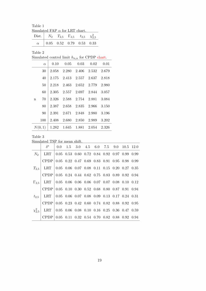
Table 1Simulated FAP 𝛼 for LRT chart.

Dist. 𝑁2 𝑇2,5 Γ2,5 𝑡2,5 𝜒22,5

𝛼 0.05 0.52 0.79 0.53 0.33

Table 2Simulated control limit ℎ𝑛,𝛼 for CPDP chart.

𝛼 0.10 0.05 0.03 0.02 0.01

30 2.058 2.280 2.406 2.532 2.679

40 2.175 2.413 2.557 2.637 2.818

50 2.218 2.463 2.652 2.779 2.980

60 2.305 2.557 2.697 2.844 3.057

n 70 2.326 2.588 2.754 2.881 3.084

80 2.387 2.658 2.835 2.966 3.150

90 2.391 2.671 2.848 2.980 3.196

100 2.408 2.680 2.850 2.989 3.202

𝑁(0, 1) 1.282 1.645 1.881 2.054 2.326

Table 3Simulated TSP for mean shift.

𝛿∗ 0.0 1.5 3.0 4.5 6.0 7.5 9.0 10.5 12.0

𝑁2 LRT 0.05 0.53 0.60 0.72 0.84 0.92 0.97 0.99 0.99

CPDP 0.05 0.22 0.47 0.69 0.83 0.91 0.95 0.98 0.99

𝑇2,5 LRT 0.05 0.06 0.07 0.08 0.11 0.15 0.20 0.27 0.35

CPDP 0.05 0.24 0.44 0.62 0.75 0.83 0.89 0.92 0.94

Γ2,5 LRT 0.05 0.06 0.06 0.06 0.07 0.07 0.08 0.10 0.12

CPDP 0.05 0.10 0.30 0.52 0.68 0.80 0.87 0.91 0.94

𝑡2,5 LRT 0.05 0.06 0.07 0.08 0.09 0.13 0.17 0.24 0.31

CPDP 0.05 0.23 0.42 0.60 0.74 0.82 0.88 0.92 0.95

𝜒22,5 LRT 0.05 0.06 0.08 0.10 0.16 0.25 0.36 0.47 0.59

CPDP 0.05 0.11 0.32 0.54 0.70 0.82 0.88 0.92 0.94

19

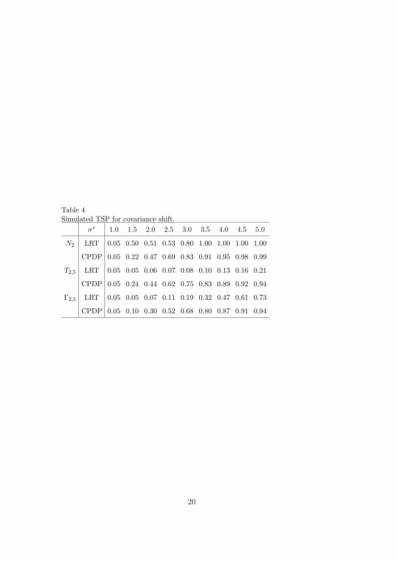
Table 4Simulated TSP for covariance shift.

𝜎∗ 1.0 1.5 2.0 2.5 3.0 3.5 4.0 4.5 5.0

𝑁2 LRT 0.05 0.50 0.51 0.53 0.80 1.00 1.00 1.00 1.00

CPDP 0.05 0.22 0.47 0.69 0.83 0.91 0.95 0.98 0.99

𝑇2,5 LRT 0.05 0.05 0.06 0.07 0.08 0.10 0.13 0.16 0.21

CPDP 0.05 0.24 0.44 0.62 0.75 0.83 0.89 0.92 0.94

Γ2,5 LRT 0.05 0.05 0.07 0.11 0.19 0.32 0.47 0.61 0.73

CPDP 0.05 0.10 0.30 0.52 0.68 0.80 0.87 0.91 0.94

20

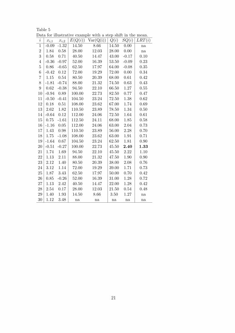
Table 5Data for illustrative example with a step shift in the mean.𝑖 𝑥𝑖,1 𝑥𝑖,2 𝐸(𝑄(𝑖)) Var(Q(i)) 𝑄(𝑖) 𝑆𝑄(𝑖) 𝐿𝑅𝑇 (𝑖)

1 -0.09 -1.32 14.50 8.66 14.50 0.00 na2 1.84 0.58 28.00 12.03 28.00 0.00 na3 0.58 0.71 40.50 14.47 43.00 -0.17 0.104 -0.36 -0.97 52.00 16.39 53.50 -0.09 0.235 0.86 -0.65 62.50 17.97 64.00 -0.08 0.356 -0.42 0.12 72.00 19.29 72.00 0.00 0.347 1.15 0.54 80.50 20.39 68.00 0.61 0.428 -1.81 -0.74 88.00 21.32 74.50 0.63 0.439 0.62 -0.38 94.50 22.10 66.50 1.27 0.5510 -0.94 0.89 100.00 22.73 82.50 0.77 0.4711 -0.50 -0.41 104.50 23.24 72.50 1.38 0.6212 0.18 0.51 108.00 23.62 67.00 1.74 0.6913 2.62 1.82 110.50 23.89 78.50 1.34 0.5014 -0.64 0.12 112.00 24.06 72.50 1.64 0.6115 0.75 -1.61 112.50 24.11 68.00 1.85 0.5816 -1.16 0.05 112.00 24.06 63.00 2.04 0.7317 1.43 0.98 110.50 23.89 56.00 2.28 0.7018 1.75 -1.08 108.00 23.62 63.00 1.91 0.7119 -1.64 0.67 104.50 23.24 62.50 1.81 0.9020 -0.51 -0.27 100.00 22.73 45.50 2.40 1.3321 1.74 1.69 94.50 22.10 45.50 2.22 1.1022 1.13 2.11 88.00 21.32 47.50 1.90 0.9023 2.12 1.40 80.50 20.39 38.00 2.08 0.7624 3.12 1.14 72.00 19.29 39.00 1.71 0.7325 1.87 3.43 62.50 17.97 50.00 0.70 0.4226 0.85 -0.26 52.00 16.39 31.00 1.28 0.7227 1.13 2.42 40.50 14.47 22.00 1.28 0.4228 2.54 0.17 28.00 12.03 21.50 0.54 0.4829 1.40 1.93 14.50 8.66 3.50 1.27 na30 1.12 3.48 na na na na na

21

Table 6Data for illustrative example with 3 increase for samples 20, 25 and 30.𝑖 𝑥𝑖,1 𝑥𝑖,2 𝐸(𝑄(𝑖)) Var(Q(i)) 𝑄(𝑖) 𝑆𝑄(𝑖) 𝐿𝑅𝑇 (𝑖)

1 -0.09 -1.32 14.50 8.66 14.50 0.00 na2 1.84 0.58 28.00 12.03 28.00 0.00 na3 0.58 0.71 40.50 14.47 44.00 -0.24 0.134 -0.36 -0.97 52.00 16.39 55.50 -0.21 0.255 0.86 -0.65 62.50 17.97 65.00 -0.14 0.406 -0.42 0.12 72.00 19.29 75.00 -0.16 0.417 1.15 0.54 80.50 20.39 72.00 0.42 0.528 -1.81 -0.74 88.00 21.32 75.00 0.61 0.519 0.62 -0.38 94.50 22.10 68.00 1.20 0.6510 -0.94 0.89 100.00 22.73 93.50 0.29 0.6011 -0.50 -0.41 104.50 23.24 85.50 0.82 0.7412 0.18 0.51 108.00 23.62 80.00 1.19 0.8513 2.62 1.82 110.50 23.89 89.00 0.90 0.6814 -0.64 0.12 112.00 24.06 85.50 1.10 0.8015 0.75 -1.61 112.50 24.11 82.00 1.27 0.7316 -1.16 0.05 112.00 24.06 80.50 1.31 0.8517 1.43 0.98 110.50 23.89 75.50 1.46 0.8818 1.75 -1.08 108.00 23.62 87.00 0.89 0.9319 -1.64 0.67 104.50 23.24 97.50 0.30 1.0920 2.49 2.73 100.00 22.73 102.50 -0.11 0.7721 0.24 0.19 94.50 22.10 82.50 0.54 0.8522 -0.37 0.61 88.00 21.32 72.50 0.73 0.9623 0.62 -0.10 80.50 20.39 52.50 1.37 1.0324 1.62 -0.36 72.00 19.29 43.50 1.48 1.0925 4.87 6.43 62.50 17.97 42.50 1.11 0.2126 -0.65 -1.76 52.00 16.39 41.00 0.67 0.2027 -0.37 0.92 40.50 14.47 33.00 0.52 0.2028 1.04 -1.33 28.00 12.03 27.00 0.08 1.7229 -0.10 0.43 14.50 8.66 3.00 1.33 na30 4.12 6.48 na na na na na

22

Table 7Data for illustrative example with gradual increase 1.5× 𝑖−20

10 for sample 𝑖, 20 ≤ 𝑖 ≤30.𝑖 𝑥𝑖,1 𝑥𝑖,2 𝐸(𝑄(𝑖)) Var(Q(i)) 𝑄(𝑖) 𝑆𝑄(𝑖) 𝐿𝑅𝑇 (𝑖)

1 -0.09 -1.32 14.50 8.66 14.50 0.00 na2 1.84 0.58 28.00 12.03 28.00 0.00 na3 0.58 0.71 40.50 14.47 44.00 -0.24 0.094 -0.36 -0.97 52.00 16.39 57.50 -0.34 0.195 0.86 -0.65 62.50 17.97 68.50 -0.33 0.306 -0.42 0.12 72.00 19.29 78.00 -0.31 0.267 1.15 0.54 80.50 20.39 76.00 0.22 0.348 -1.81 -0.74 88.00 21.32 80.50 0.35 0.319 0.62 -0.38 94.50 22.10 72.50 1.00 0.4110 -0.94 0.89 100.00 22.73 89.00 0.48 0.2911 -0.50 -0.41 104.50 23.24 80.00 1.05 0.4012 0.18 0.51 108.00 23.62 75.00 1.40 0.4513 2.62 1.82 110.50 23.89 87.00 0.98 0.3114 -0.64 0.12 112.00 24.06 80.50 1.31 0.3815 0.75 -1.61 112.50 24.11 79.00 1.39 0.3016 -1.16 0.05 112.00 24.06 75.50 1.52 0.3617 1.43 0.98 110.50 23.89 70.00 1.69 0.3518 1.75 -1.08 108.00 23.62 77.50 1.29 0.3419 -1.64 0.67 104.50 23.24 76.50 1.21 0.3820 -2.01 -1.77 100.00 22.73 77.50 0.99 0.6821 0.39 0.34 94.50 22.10 57.50 1.67 0.7122 -0.07 0.91 88.00 21.32 48.00 1.88 0.7823 1.07 0.35 80.50 20.39 31.00 2.43 0.7524 2.22 0.24 72.00 19.29 31.00 2.13 0.7225 1.12 2.68 62.50 17.97 44.00 1.03 0.3926 0.25 -0.86 52.00 16.39 28.50 1.43 0.6027 0.68 1.97 40.50 14.47 17.00 1.62 0.4628 2.24 -0.13 28.00 12.03 16.00 1.00 0.5629 1.25 1.78 14.50 8.66 3.00 1.33 na30 1.12 3.48 na na na na na

23

Table 8Data for illustrative example with mean shift, variance shift and simultaneous shift.

with subtracting mean without subtracting meani mean variance simultaneous mean variance simultaneous

1 0.00 0.00 0.00 0.00 0.00 0.002 0.00 0.00 0.00 0.00 0.00 0.003 0.07 -0.07 0.03 -0.17 -0.07 -0.034 0.12 -0.12 0.46 -0.09 -0.03 0.125 0.17 -0.14 0.58 -0.08 0.03 0.196 0.08 -0.29 0.52 0.00 0.16 0.297 0.69 0.25 0.98 0.61 0.76 0.938 0.63 0.19 1.20 0.63 0.89 0.969 0.97 0.52 1.52 1.27 1.52 1.5810 1.28 0.97 1.89 0.77 1.19 1.2311 1.48 1.40 2.35 1.38 1.74 1.8312 1.88 1.88 2.48 1.74 2.14 2.2413 1.30 1.49 2.51 1.34 1.76 2.0514 1.31 2.02 2.72 1.64 2.04 2.4115 1.47 2.22 3.24 1.85 2.24 2.7416 1.33 2.22 3.26 2.04 2.35 2.9717 1.80 2.66 2.99 2.28 2.57 2.8018 1.10 2.16 2.52 1.91 2.24 2.9219 0.30 2.00 2.00 1.81 1.98 2.8020 -0.20 1.25 1.28 2.40 1.96 3.1221 0.36 1.95 1.97 2.22 2.72 3.0522 0.26 2.11 2.11 1.90 2.44 2.8423 1.10 2.35 2.28 2.08 2.65 2.6524 0.52 1.37 1.53 1.71 2.51 2.2025 0.47 1.61 1.59 0.70 1.89 1.2826 -0.21 0.18 0.37 1.28 1.56 1.5627 0.52 0.69 1.00 1.28 1.11 1.3828 -1.16 0.21 -0.50 0.54 0.50 0.7529 -1.68 -1.68 -1.56 1.27 1.33 1.33

24

0 10 20 30 40 50

−2

−1

01

23

i

SQ

(i)

h56,0.05 = 2.519i=24

(a)

25 30 35 40 45 50 55

−2

−1

01

23

i

SQ

(i)

h32,0.05 = 2.306i=42

(b)

Fig. 1. 𝑆𝑄(𝑖) values for the gravel data.

25