Multivariate Approximation and Matrix Calculus · PDF fileMultivariate Approximation and Matrix Calculus Mathematical Modeling and Simulation; Module 2: Matrix Calculus and Optimization

Multivariate Approximation and Matrix Calculus

Mathematical Modeling and Simulation; Module 2: Matrix Calculus and Optimization Page 1 Chapter 1: Introduction to Linear Regression

Introduction Taylor series is a representation of a function as an infinite sum of terms

that are calculated from the values of the function's derivatives at a single point. Any finite number of initial terms of the Taylor series of a function is

called a Taylor polynomial. In single variable calculus, Taylor polynomial of

n degrees is used to approximate an (n+1)-order differentiable function

and the error of the approximation can be estimated by the (n+1)-th term

of the Taylor series. By introducing vector and matrix calculus notations,

we can express the same idea for multivariate functions and vector

functions.

Applications Because all numbers that can be represented by finite digits are rational

numbers, the numerical computation of an irrational function at a

particular point is almost always approximated. The first order and second

order of Taylor polynomials are most frequently selected as the proper

rational function to approximate irrational functions. This idea is called

linear and quadratic approximation in calculus, respectively. In addition,

the quadratic approximation is also used to in optimization because local

maximum or minimum occurs at the critical points where the second term

(first derivatives) of the Taylor polynomial is zero and the third term

(second derivatives) are definitely positive or negative. In order to obtain

the first or second order Taylor polynomial, we compute the coefficients of

Taylor series by calculating the first and second derivatives of the original

function. When we move towards the advanced mathematical applications

(temperature in 4 dimensional temporal-spatial space and vector field of

moving hurricane centers), we need to use multivariate (vector) functions,

instead of single variable functions. In terms of the linear and quadratic

approximation, we still use the idea of first and second order Taylor

polynomials. However, we need to first generalize the concepts of the first

and second order derivatives in multivariate context to obtain the

coefficients of Taylor polynomials. Then, we can obtain the multivariate

Taylor polynomial to approximate an irrational multivariate function.

Goal and

Objectives

Reflection

Questions

We will extend the concepts of the first and second derivatives in the

context of multivariate functions and apply these concepts to obtain the

first and second order Taylor polynomials for multivariate functions. Our

objectives are to learn the following concepts and associative formulas:

1. Gradient vector and matrix calculus

2. Linear approximation multivariate functions

3. Quadratic Taylor formula for multivariate functions

4. Use MATLAB to compute the Taylor series

In history, mathematicians had to spend years calculating the value tables

of many special functions such as Bessel functions and Legendre function.

Nowadays, it is a trivial click to use MATLAB to estimate the value of any

known function at any particular point. It seems that it is unnecessary to

learn the approximating techniques. But, think about these questions.

1. How do you render a smooth surface to graph a multivariate function?

2. Why we only need to consider the first and second derivative to find

optimal solutions to most applications?

3. What does an IMU (Inertial Measurement Unit) for robotic navigation

system need to sense in order to estimate its own positions?

http://en.wikipedia.org/wiki/Function_(mathematics)

http://en.wikipedia.org/wiki/Series_(mathematics)

http://en.wikipedia.org/wiki/Derivative

http://en.wikipedia.org/wiki/Taylor_polynomial



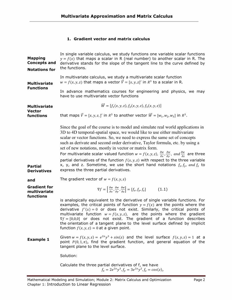
1. Gradient vector and matrix calculus

Mapping

Concepts and

Notations for

Multivariate

Functions

Multivariate

Vector

functions

Partial

Derivatives

and

Gradient for

multivariate

functions

In single variable calculus, we study functions one variable scalar functions that maps a scalar in R (real number) to another scalar in R. The

derivative stands for the slope of the tangent line to the curve defined by

the functions.

In multivariate calculus, we study a multivariate scalar function

that maps a vector in to a scalar in R.

In advance mathematics courses for engineering and physics, we may

have to use multivariate vector functions

that maps in to another vector in .

Since the goal of the course is to model and simulate real world applications in

3D to 4D temporal-spatial space, we would like to use either multivariate

scalar or vector functions. So, we need to express the same set of concepts

such as derivate and second order derivative, Taylor formula, etc. by using a

set of new notations, mostly in vector or matrix form.

For multivariate scalar valued function

are three

partial derivatives of the function with respect to the three variable

x, y, and z. Sometime, we use the short hand notations to

express the three partial derivatives.

The gradient vector of

[

] (1.1)

is analogically equivalent to the derivative of single variable functions. For examples, the critical points of function are the points where the

derivative or does not exist. Similarly, the critical points of

multivariate function are the points where the gradient

or does not exist. The gradient of a function describes

the orientation of a tangent plane to the level surface defined by implicit

function at a given point.

Example 1

Given and the level surface at a

point , find the gradient function, and general equation of the

tangent plane to the level surface.

Solution:

Calculate the three partial derivatives of f, we have ,

http://en.wikipedia.org/wiki/Orientation_(mathematics)

http://en.wikipedia.org/wiki/Tangent_plane



Component-

wise

differentiation

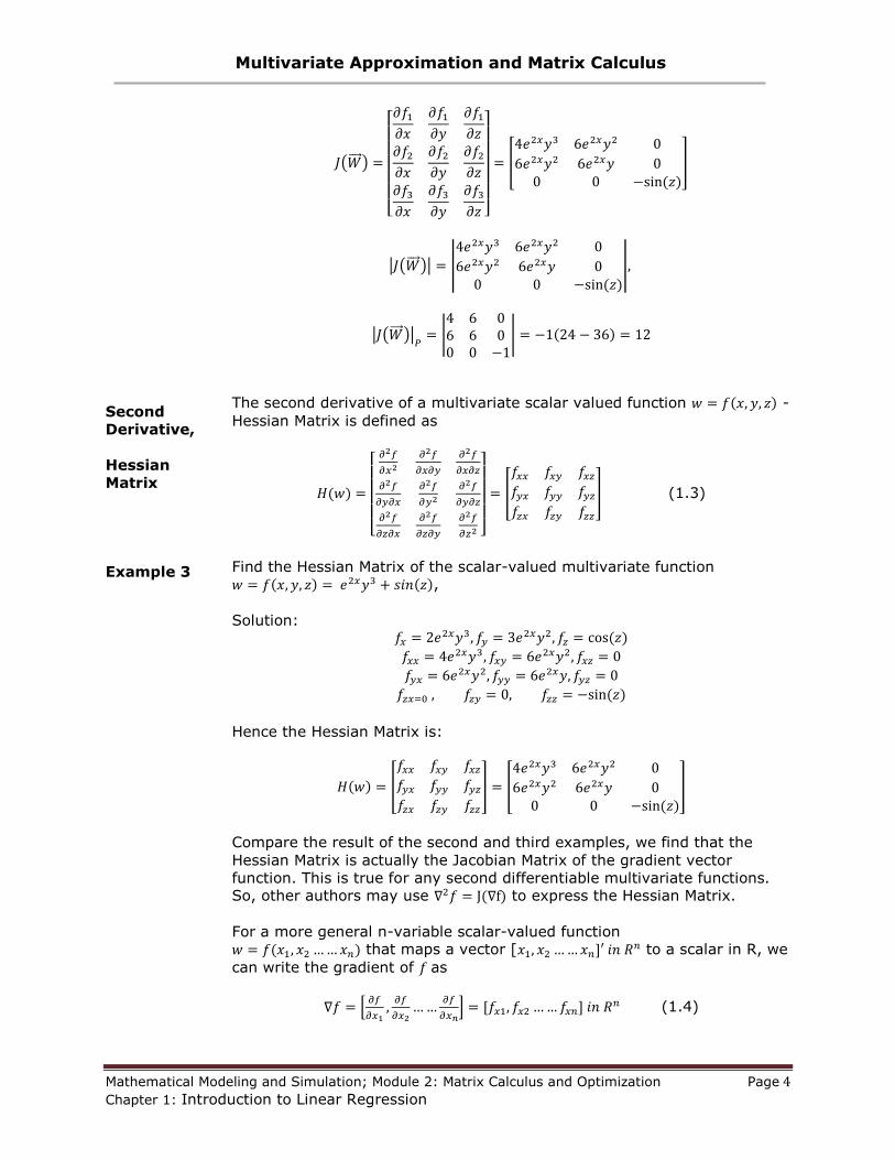
Jacobian

Matrix and

Jacobian

determinant

Example 2

Therefore, the gradient is:

,

Substitute the component values of P to the gradient, we have

, which is the normal vector of the tangent plane to the level

surface. Hence, the point normal equation of the tangent plane is:

– .

The general equation is

– .

single variable t (typically stands for time in dynamic systems) in R to a

vector in . The derivative is the

directional vector of the tangent line of the curve defined by the vector-

valued function at a particular point. . The

operations above are called as component-wise differentiations.

For multivariate vector valued functions

that maps in to another vector in , we can

define the so called Jacobian Matrix and Jacobian determinant are defined

as follows

[

]

and | | ||

|| (1.2)

Notice that each row of the 3X3 matrix is the gradient of each component

scalar valued function and each column is the partial derivatives of the

vector function with respect to an individual variable. The Jacobian of a

function describes the orientation of a tangent plane to the function at a

given point. In this way, the Jacobian generalizes the gradient of a scalar

valued function of multiple variables which itself generalizes the derivative

of a scalar-valued function of a scalar.

Notice that gradient in example 1 above is a vector function, find the

Jacobian matrix as a matrix function and Jacobian determinant of the gradient at point .

.

Solution: For vector valued function

http://en.wikipedia.org/wiki/Orientation_(mathematics)

http://en.wikipedia.org/wiki/Tangent_plane

http://en.wikipedia.org/wiki/Gradient



( )

[

]

[

]

| ( )| |

|

| ( )|

|

|

Second

Derivative,

Hessian

Matrix

Example 3

The second derivative of a multivariate scalar valued function - Hessian Matrix is defined as

[

]

[

] (1.3)

Find the Hessian Matrix of the scalar-valued multivariate function ,

Solution:

Hence the Hessian Matrix is:

[

] [

]

Compare the result of the second and third examples, we find that the

Hessian Matrix is actually the Jacobian Matrix of the gradient vector

function. This is true for any second differentiable multivariate functions. So, other authors may use to express the Hessian Matrix.

For a more general n-variable scalar-valued function that maps a vector [ to a scalar in R, we

can write the gradient of as

[

] (1.4)



The Hessian Matrix as the following matrix

[

]

(1.5)

Self-Check

Exercises

(1) Find the gradient and Hessian Matrix of the function at point .

(2) Find the Jacobian matrix and the Jacobian determinant of the vector function at point .



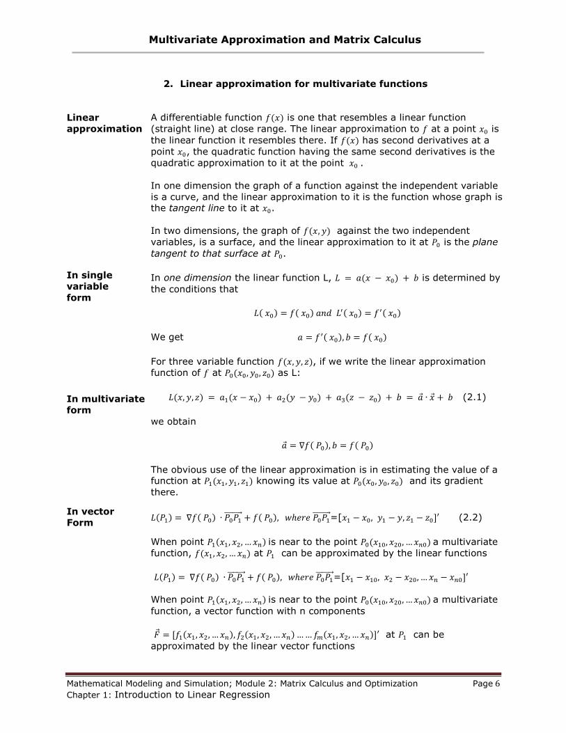
2. Linear approximation for multivariate functions

Linear

approximation

In single

variable

form

In multivariate

form

In vector

Form

A differentiable function is one that resembles a linear function

(straight line) at close range. The linear approximation to at a point is

the linear function it resembles there. If has second derivatives at a

point , the quadratic function having the same second derivatives is the

quadratic approximation to it at the point .

In one dimension the graph of a function against the independent variable

is a curve, and the linear approximation to it is the function whose graph is the tangent line to it at .

In two dimensions, the graph of against the two independent

variables, is a surface, and the linear approximation to it at is the plane

tangent to that surface at .

In one dimension the linear function L, is determined by

the conditions that

We get

For three variable function , if we write the linear approximation

function of at as L:

(2.1)

we obtain

The obvious use of the linear approximation is in estimating the value of a function at knowing its value at and its gradient

there.

=[ (2.2)

When point is near to the point a multivariate

function, at can be approximated by the linear functions

=[ When point is near to the point a multivariate

function, a vector function with n components

at can be

approximated by the linear vector functions



=[

Where is the Jacobian Matrix of the function F at point .

We can simply regard the last formula as a list of m previous formulas.

Use the linear approximation of √

√ √

at point to

estimate √

√ √

,

Solution: The value of the function at can be approximated

by the value of L at , where the linear function L is given by eq.

(1.2).

[

] [

]

=[

]

,

=[ ,

[

]

Use Maple, you will find the error is

29.30162037-29.27618252=0.02543785.

Self-Check

Exercises

(3) Use the linear approximation of √

√ at point to

estimate √

√ ,

(4) Use the linear approximation of at point

to estimate



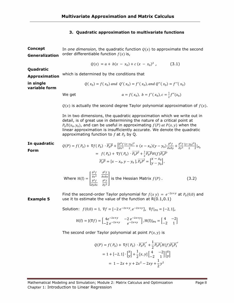
3. Quadratic approximation to multivariate functions

Concept

Generalization

Quadratic

Approximation

in single

variable form

In quadratic

Form

Example 5

In one dimension, the quadratic function to approximate the second

order differentiable function is,

, (3.1)

which is determined by the conditions that

We get

is actually the second degree Taylor polynomial approximation of .

In in two dimensions, the quadratic approximation which we write out in

detail, is of great use in determining the nature of a critical point at

, and can be useful in approximating when the

linear approximation is insufficiently accurate. We denote the quadratic approximating function to at by Q.

[

]

[

]

Where [

] is the Hessian Matrix . (3.2)

Find the second-order Taylor polynomial for at and

use it to estimate the value of the function at R(0.1,0.1)

Solution: ], ,

[

] [

]

The second order Taylor polynomial at point is

[ ]

[

] [ ]

http://www-math.mit.edu/~djk/18_022/chapter04/supplement01.html

http://www-math.mit.edu/~djk/18_022/chapter04/supplement01.html



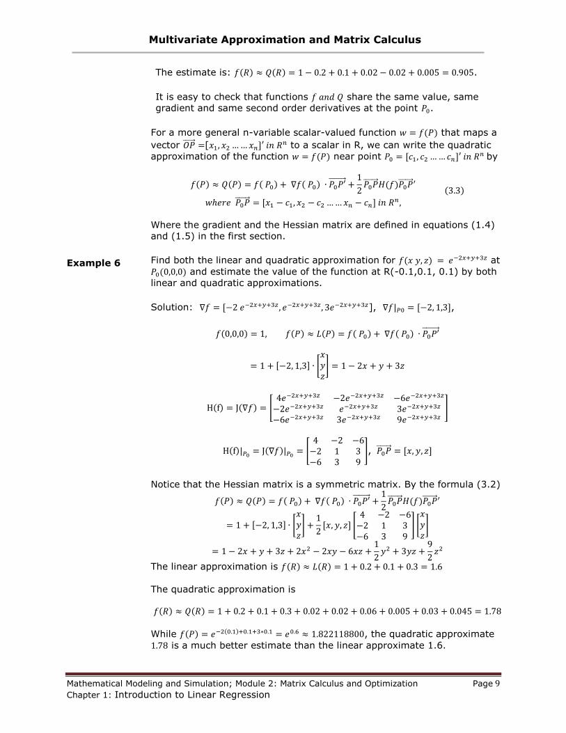
Example 6

The estimate is: .

It is easy to check that functions share the same value, same

gradient and same second order derivatives at the point .

For a more general n-variable scalar-valued function that maps a

vector [ to a scalar in R, we can write the quadratic

approximation of the function near point by

Where the gradient and the Hessian matrix are defined in equations (1.4)

and (1.5) in the first section.

Find both the linear and quadratic approximation for at

and estimate the value of the function at R(-0.1,0.1, 0.1) by both

linear and quadratic approximations.

Solution: ], ,

[ ]

[

]

[

],

Notice that the Hessian matrix is a symmetric matrix. By the formula (3.2)

[ ]

[

] [ ]

The linear approximation is

The quadratic approximation is

While , the quadratic approximate

is a much better estimate than the linear approximate 1.6.



Self-Check

Exercises

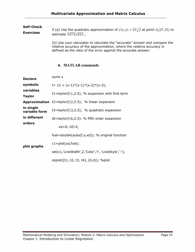
5.(a) Use the quadratic approximation of √

√ at point to

estimate √

√ ,

(b) Use your calculator to calculate the “accurate” answer and compare the

relative accuracy of the approximation, where the relative accuracy is defined as the ratio of the error against the accurate answer.

4. MATLAB commands

Declare

symbolic

variables

Taylor

Approximation

in single

variable form

in different

orders

plot graphs

syms x

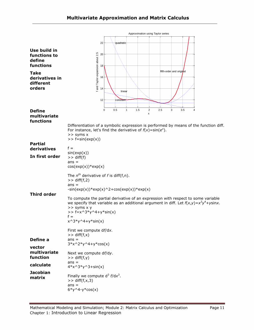
f= 12 + (x-1)*(x-1)*(x-2)*(x-3);

t1=taylor(f,1,2.5); % expansion with first term

t2=taylor(f,2,2.5); % linear expansion

t3=taylor(f,3,2.5); % quadratic expansion

t6=taylor(f,6,2.5); % fifth order expansion

xd=0:.05:4;

fval=double(subs(f,x,xd)); % original function

c1=plot(xd,fval);

set(c1,'LineWidth',2,'Color','r', 'LineStyle','-');

ezplot([t1, t2, t3, t4], [0,4]); %plot



Use build in

functions to

define

functions

Take

derivatives in

different

orders

Define

multivariate

functions

Partial

derivatives

In first order

Third order

Define a

vector

multivariate

function

calculate

Jacobian

matrix

Differentiation of a symbolic expression is performed by means of the function diff. For instance, let's find the derivative of f(x)=sin(ex). >> syms x >> f=sin(exp(x)) f = sin(exp(x))

>> diff(f) ans = cos(exp(x))*exp(x) The nth derivative of f is diff(f,n).

>> diff(f,2)

ans = -sin(exp(x))*exp(x)^2+cos(exp(x))*exp(x) To compute the partial derivative of an expression with respect to some variable we specify that variable as an additional argument in diff. Let f(x,y)=x3y4+ysinx. >> syms x y >> f=x^3*y^4+y*sin(x)

f = x^3*y^4+y*sin(x) First we compute df/dx. >> diff(f,x) ans = 3*x^2*y^4+y*cos(x)

Next we compute df/dy. >> diff(f,y) ans = 4*x^3*y^3+sin(x)

Finally we compute d3 f/dx3. >> diff(f,x,3) ans = 6*y^4-y*cos(x)

0 0.5 1 1.5 2 2.5 3 3.5 4

12

14

16

18

20

22

x

Approximation using Taylor series

constant

linear

fifth-order and original

quadratic

f and T

aylo

r expansio

n a

bout

2.5



Jacobian of

linear

transformation

matrix is

the coefficient

Matrix of the

transformation

Find critical

points

Hession matrix

is the jacobian

of the jacobian

matrix

The Jacobian matrix of a function f:Rn -> Rm can be found directly using the

jacobian function. For example, let f:R2 -> R3 be defined by f(x,y)=(sin(xy),x2+y2,3x-2y).

>> f=[sin(x*y); x^2+y^2; 3*x-2*y] f = [ sin(y*x)] [ x^2+y^2] [ 3*x-2*y]

>> Jf=jacobian(f) Jf = [ cos(y*x)*y, cos(y*x)*x] [ 2*x, 2*y] [ 3, -2]

In the case of a linear transformation, the Jacobian is quite simple.

>> A=[11 -3 14 7;5 7 9 2;8 12 -6 3] A = 11 -3 14 7 5 7 9 2 8 12 -6 3 >> syms x1 x2 x3 x4 >> x=[x1;x2;x3;x4]

x = [ x1] [ x2] [ x3] [ x4] >> T=A*x

T = [ 11*x1-3*x2+14*x3+7*x4]

[ 5*x1+7*x2+9*x3+2*x4] [ 8*x1+12*x2-6*x3+3*x4] Now let's find the Jacobian of T. >> JT=jacobian(T)

JT = [ 11, -3, 14, 7] [ 5, 7, 9, 2] [ 8, 12, -6, 3] The Jacobian of T is precisely A.

Next suppose f:Rn -> R is a scalar valued function. Then its Jacobian is just its

gradient. (Well, almost. Strictly speaking, they are the transpose of one another since the Jacobian is a row vector and the gradient is a column vector.) For example, let f(x,y)=(4x2-1)e-x2-y2.

>> syms x y real

>> f=(4*x^2-1)*exp(-x^2-y^2) f = (4*x^2-1)*exp(-x^2-y^2) >> gradf=jacobian(f) gradf = [ 8*x*exp(-x^2-y^2)-2*(4*x^2-1)*x*exp(-x^2-y^2), -2*(4*x^2-1)*y*exp(-x^2-y^2)]

Next we use solve to find the critical points of f.



Calculate the

determinant to

find maximum

or minimum

>> S=solve(gradf(1),gradf(2));

>> [S.x S.y] ans =

[ 0, 0] [ 1/2*5^(1/2), 0] [ -1/2*5^(1/2), 0] Thus the critical points are (0,0), (Ö5/2,0) and (-Ö5/2,0).

The Hessian of a scalar valued function f:Rn -> R is the n×n matrix of second order

partial derivatives of f. In MATLAB we can obtain the Hessian of f by computing the Jacobian of the Jacobian of f. Consider once again the function f(x,y)=(4x2-1)e-x2-y2.

>> syms x y real >> Hf=jacobian(jacobian(f));

>> Hf=simple(Hf)

Hf = [2*exp(-x^2-y^2)*(2*x+1)*(2*x-1)*(2*x^2-5), 4*x*y*exp(-x^2-y^2)*(-5+4*x^2)] [4*x*y*exp(-x^2-y^2)*(-5+4*x^2), 2*exp(-x^2-y^2)*(-1+2*y^2)*(2*x+1)*(2*x-1)] We can now use the Second Derivative Test to determine the type of each critical

point of f found above. >> subs(Hf,{x,y},{0,0}) ans = 10 0 0 2 >> subs(Hf,{x,y},{1/2*5^(1/2),0})

ans = -5.7301 0

0 -2.2920 >> subs(Hf,{x,y},{-1/2*5^(1/2),0}) ans = -5.7301 0 0 -2.2920

Thus f has a local minimum at (0,0) and local maxima at the other two critical points. Evaluating f at the critical points gives the maximum and minimum values of f. >> subs(f,{x,y},{0,0}) ans = -1

>> subs(f,{x,y},{'1/2*5^(1/2)',0}) ans = 4*exp(-5/4) >> subs(f,{x,y},{'-1/2*5^(1/2)',0})

ans = 4*exp(-5/4)

Thus the minimum value of f is f(0,0)=-1 and the maximum value is

√ √ .

The graph of f is shown in figure 1.



Review

Exercises

1. Use your scientific calculator to find the answers

(a) Find the linear approximation of at point , use what you find to estimate . (b) Find the quadratic approximation of at point and use what you find estimate .

(b) Use your calculator to calculate the “accurate” answer and compare

the relative accuracy of the two approximations above, where the

relative accuracy is defined as the ratio of the error against the

accurate answer.

2. Use MATLAB command to find the answers to the problem 1.



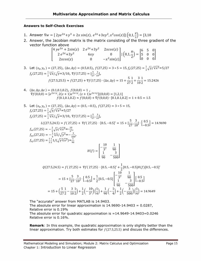
Answers to Self-Check Exercises

1. Answer (

)

2. Answer, the Jacobian matrix is the matrix consisting of the three gradient of the

vector function above

[

] (

) [

]

3. Let , ,

√ √

=

√

√ = ,

,

4. , ,

5. Let , ,

√ √

=

√

√ = ,

,

[

]

√ √

=-

,

√

√ =

,

√ √

=

[

]

[

]

[

] [

]

(

)

(

) (

)

(

)

(

) (

)

The “accurate” answer from MATLAB is 14.9403.

The absolute error for linear approximation is 14.9690-14.9403 = 0.0287,

Relative error is 0.19%

The absolute error for quadratic approximation is =14.9649-14.9403=0.0246

Relative error is 0.16%.

Remark: In this example, the quadratic approximation is only slightly better than the

linear approximation. Try both estimates for and discuss the differences.

Documents

Multivariate Approximation and Matrix Calculus · PDF fileMultivariate Approximation and Matrix Calculus Mathematical Modeling and Simulation; Module 2: Matrix Calculus and Optimization