Embed Size (px)
Citation preview

Matrix Approximation for Large-scale Learningby
Ameet Talwalkar
A dissertation submitted in partial fulfillmentof the requirements for the degree of
Doctor of PhilosophyDepartment of Computer Science
Courant Institute of Mathematical SciencesNew York University
May 2010
Mehryar Mohri—Advisor

c© Ameet TalwalkarAll Rights Reserved, 2010


For Aai and Baba
iv

Acknowledgments
I would first like to thank my advisor, Mehryar Mohri, for his guidancethroughout my doctoral studies. He gave me an opportunity to pursue aPhD, patiently taught me about the field of machine learning and guided metowards exciting research questions. He also introduced me to my mentors andcollaborators at Google Research, Sanjiv Kumar and Corinna Cortes, both ofwhom have been tremendous role models for me throughout my studies. Iwould also like to thank the final two members of my thesis committee, Den-nis Shasha and Mark Tygert, as well as Subhash Khot, who sat on my DQEand thesis proposal, for their encouragement and helpful advice.
During my time at Courant and my summers at Google, I have had thegood fortune to work and interact with several other exceptional people. Inparticular, I would like to thank Eugene Weinstein, Ameesh Makadia, Cyril Al-lauzen, Dejan Jovanovic, Shaila Musharoff, Ashish Rastogi, Rosemary Amico,Michael Riley, Henry Rowley and Jeremy Shute for helping me along the wayand making my studies and research more enjoyable over these past four years.I would especially like to thank my partner in crime, Afshin Rostamizadeh, forbeing a supportive officemate and a considerate friend throughout our count-less hours working together.
Last, but not least, I would like to thank my friends and family for theirunwavering support. In particular, I have consistently drawn strength frommy lovely girlfriend Jessica, my brother Jaideep, my sister-in-law Kristen andthe three cutest little men in the world, my nephews Kavi, Nayan and Dev.And to my parents, Rohini and Shrirang, to whom this thesis is dedicated,I am infinitely grateful. They are my sources of inspiration and my greatestteachers, and any achievement I may have is a credit to them. Thank you,Aai and Baba.
v

Abstract
Modern learning problems in computer vision, natural language processing,computational biology, and other areas are often based on large data setsof tens of thousands to millions of training instances. However, several stan-dard learning algorithms, such as kernel-based algorithms, e.g., Support VectorMachines, Kernel Ridge Regression, Kernel PCA, do not easily scale to suchorders of magnitude. This thesis focuses on sampling-based matrix approxima-tion techniques that help scale kernel-based algorithms to large-scale datasets.We address several fundamental theoretical and empirical questions including:
1. What approximation should be used? We discuss two common sampling-based methods, providing novel theoretical insights regarding their suit-ability for various applications and experimental results motivated bythis theory. Our results show that one of these methods, the Nystrommethod, is superior in the context of large-scale learning.
2. Do these approximations work in practice? We show the effectiveness ofapproximation techniques on a variety of problems. In the largest studyto-date for manifold learning, we use the Nystrom method to extract low-dimensional structure from high-dimensional data to effectively clusterface images. We also report good empirical results for Kernel RidgeRegression and Kernel Logistic Regression.
3. How should we sample columns? A key aspect of sampling-based algo-rithms is the distribution according to which columns are sampled. Westudy both fixed and adaptive sampling schemes as well as a promisingensemble technique that can be easily parallelized and generates superiorapproximations, both in theory and in practice.
4. How well do these approximations work in theory? We provide theoret-ical analyses of the Nystrom method to understand when this technique
vi

should be used. We present guarantees on approximation accuracy basedon various matrix properties and analyze the effect of matrix approxi-mation on actual kernel-based algorithms.
This work has important consequences for the machine learning commu-nity since it extends to large-scale applications the benefits of kernel-basedalgorithms. The crucial aspect of this research, involving low-rank matrixapproximation, is of independent interest within the field of linear algebra.
vii

Contents
Dedication . . . . . . . . . . . . . . . . . . . . . . . . . . . . . . . . ivAcknowledgments . . . . . . . . . . . . . . . . . . . . . . . . . . . . vAbstract . . . . . . . . . . . . . . . . . . . . . . . . . . . . . . . . . viList of Figures . . . . . . . . . . . . . . . . . . . . . . . . . . . . . . xList of Tables . . . . . . . . . . . . . . . . . . . . . . . . . . . . . . xiv
1 Introduction 11.1 Motivation . . . . . . . . . . . . . . . . . . . . . . . . . . . . . 11.2 Related Work . . . . . . . . . . . . . . . . . . . . . . . . . . . 31.3 Contributions . . . . . . . . . . . . . . . . . . . . . . . . . . . 5
2 Low Rank Approximations 72.1 Preliminaries . . . . . . . . . . . . . . . . . . . . . . . . . . . 7
2.1.1 Notation . . . . . . . . . . . . . . . . . . . . . . . . . . 72.1.2 Nystrom method . . . . . . . . . . . . . . . . . . . . . 82.1.3 Column-sampling method . . . . . . . . . . . . . . . . 9
2.2 Nystrom vs Column-sampling . . . . . . . . . . . . . . . . . . 92.2.1 Singular values and singular vectors . . . . . . . . . . . 102.2.2 Low-rank approximation . . . . . . . . . . . . . . . . . 102.2.3 Empirical comparison . . . . . . . . . . . . . . . . . . . 15
2.3 Summary . . . . . . . . . . . . . . . . . . . . . . . . . . . . . 20
3 Applications 213.1 Large-scale Manifold Learning . . . . . . . . . . . . . . . . . . 21
3.1.1 Manifold learning . . . . . . . . . . . . . . . . . . . . . 243.1.2 Approximation experiments . . . . . . . . . . . . . . . 263.1.3 Large-scale learning . . . . . . . . . . . . . . . . . . . . 273.1.4 Manifold evaluation . . . . . . . . . . . . . . . . . . . . 33
3.2 Woodbury Approximation . . . . . . . . . . . . . . . . . . . . 38
viii

3.2.1 Nystrom Logistic Regression . . . . . . . . . . . . . . . 393.2.2 Kernel Ridge Regression . . . . . . . . . . . . . . . . . 42
3.3 Summary . . . . . . . . . . . . . . . . . . . . . . . . . . . . . 44
4 Sampling Schemes 454.1 Fixed Sampling . . . . . . . . . . . . . . . . . . . . . . . . . . 45
4.1.1 Datasets . . . . . . . . . . . . . . . . . . . . . . . . . . 464.1.2 Experiments . . . . . . . . . . . . . . . . . . . . . . . . 47
4.2 Adaptive Sampling . . . . . . . . . . . . . . . . . . . . . . . . 494.2.1 Adaptive Nystrom sampling . . . . . . . . . . . . . . . 504.2.2 Experiments . . . . . . . . . . . . . . . . . . . . . . . . 52
4.3 Ensemble Sampling . . . . . . . . . . . . . . . . . . . . . . . . 554.3.1 Ensemble Woodbury approximation . . . . . . . . . . . 574.3.2 Experiments . . . . . . . . . . . . . . . . . . . . . . . . 58
4.4 Summary . . . . . . . . . . . . . . . . . . . . . . . . . . . . . 65
5 Theoretical Analysis 665.1 Nystrom Analysis . . . . . . . . . . . . . . . . . . . . . . . . . 68
5.1.1 Standard Nystrom method . . . . . . . . . . . . . . . . 695.1.2 Ensemble Nystrom method . . . . . . . . . . . . . . . . 70
5.2 Coherence-based Bounds . . . . . . . . . . . . . . . . . . . . . 725.2.1 Coherence . . . . . . . . . . . . . . . . . . . . . . . . . 725.2.2 Low-rank, low-coherence bounds . . . . . . . . . . . . . 735.2.3 Experiments . . . . . . . . . . . . . . . . . . . . . . . . 77
5.3 Kernel Stability . . . . . . . . . . . . . . . . . . . . . . . . . . 815.3.1 Kernel Ridge Regression . . . . . . . . . . . . . . . . . 825.3.2 Support Vector Machines . . . . . . . . . . . . . . . . . 835.3.3 Support Vector Regression . . . . . . . . . . . . . . . . 885.3.4 Graph Laplacian regularization algorithms . . . . . . . 895.3.5 Kernel Principal Component Analysis . . . . . . . . . . 915.3.6 Application to Nystrom method . . . . . . . . . . . . . 96
5.4 Summary . . . . . . . . . . . . . . . . . . . . . . . . . . . . . 97
6 Conclusion 99Bibliography . . . . . . . . . . . . . . . . . . . . . . . . . . . . . . 102
ix

List of Figures
2.1 Differences in accuracy between Nystrom and Column-Sampling.Values above zero indicate better performance of Nystrom andvice-versa. (a) Top 100 singular values with l = n/10. (b)Top 100 singular vectors with l = n/10. (c) Comparison usingorthogonalized Nystrom singular vectors. . . . . . . . . . . . . 17
2.2 Performance accuracy of various matrix projection approxima-tions with k = 100. Values below zero indicate better perfor-mance of the Column-sampling method. (a) Nystrom versusColumn-sampling. (b) Orthonormal Nystrom versus Column-sampling. . . . . . . . . . . . . . . . . . . . . . . . . . . . . . 18
2.3 Performance accuracy of spectral reconstruction approximationsfor different methods with k = 100. Values above zero indicatebetter performance of the Nystrom method. (a) Nystrom versusColumn-sampling. (b) Nystrom versus Orthonormal Nystrom. 18
2.4 Properties of spectral reconstruction approximations. (a) Dif-ference in spectral reconstruction accuracy between Nystromand Column-sampling for various k and fixed l. Values abovezero indicate better performance of Nystrom method. (a) Per-centage of columns (l/n) needed to achieve 75% relative accu-racy for Nystrom spectral reconstruction as a function of n. . 19
3.1 Embedding accuracy of Nystrom and Column-Sampling. Valuesabove zero indicate better performance of Nystrom and vice-versa. . . . . . . . . . . . . . . . . . . . . . . . . . . . . . . . 27
3.2 Visualization of neighbors for Webfaces-18M. The first image ineach row is the target, and the next five are its neighbors. . . 30
3.3 A few random samples from the largest connected componentof the Webfaces-18M neighborhood graph. . . . . . . . . . . . 31
x

3.4 Visualization of disconnected components of the neighborhoodgraphs from Webfaces-18M (top row) and from PIE-35K (bot-tom row). The neighbors for each of these images are all withinthis set, thus making the entire set disconnected from the restof the graph. Note that these images are not exactly the same. 31
3.5 Visualization of disconnected components containing exactlyone image. Although several of the images above are not faces,some are actual faces, suggesting that certain areas of the facemanifold are not adequately sampled by Webfaces-18M. . . . . 32
3.6 Optimal 2D projections of PIE-35K where each point is colorcoded according to its pose label. Top Left: PCA projectionstend to spread the data to capture maximum variance, TopRight: Isomap projections with Nystrom approximation tend toseparate the clusters of different poses while keeping the clusterof each pose compact, Bottom Left: Isomap projections withColumn-sampling approximation have more overlap than withNystrom approximation. Bottom Right: Laplacian Eigenmapsprojects the data into a very compact range. . . . . . . . . . 36
3.7 2D embedding of Webfaces-18M using Nystrom Isomap (Toprow). Darker areas indicate denser manifold regions. Top Left:Face samples at different locations on the manifold. Top Right:Approximate geodesic paths between celebrities. The corre-sponding shortest-paths are shown in the bottom four rows. . 37
3.8 Pose classification experiments for a set of 2.8K faces imageswith two similar poses. (a) Classification performance for Ker-nel Logistic Regression with empirical kernel map using linearand RBF kernels. (b) Relative classification performance forKernel Logistic Regression with empirical kernel map using theNystrom approximation with different percentages of sampledcolumns. Results are reported in comparison to the perfor-mance obtained using the standard Newton method. (c) Tim-ing comparison for the same experiments as in (b), where ‘Full’corresponds to the standard Newton method. . . . . . . . . . 40
xi

3.9 Average absolute error of the Kernel Ridge Regression hypoth-esis, h′(·), generated from the Nystrom approximation, K, as a
function of relative spectral distance ‖K−K‖2/‖K‖2. For eachdataset, the reported results show the average absolute error asa function of relative spectral distance for both the full datasetand for a subset of the data containing n = 2000 points. Re-sults for the same value of n are connected with a line. Thedifferent points along the lines correspond to various numbersof sampled columns, i.e., l ranging from 1% to 50% of l. . . . 43
4.1 (a) Nystrom relative accuracy for various sampling techniqueson PIE-7K. (b) Nystrom relative accuracy for various samplingmethods for two values of l/n with k = 100. Values in paren-theses show standard deviations for 10 different runs for a fixedl. ‘+Rep’ denotes sampling with replacement. No error (‘-’) isreported for diagonal sampling with RBF kernels since diagonalsampling is equivalent to uniform sampling in this case. . . . . 48
4.2 Comparison of uniform sampling with and without replacementmeasured by the difference in relative accuracy. (a) Improve-ment in relative accuracy for PIE-7K when sampling withoutreplacement. (b) Improvement in relative accuracy when sam-pling without replacement across all datasets for various l/npercentages. . . . . . . . . . . . . . . . . . . . . . . . . . . . 49
4.3 The adaptive sampling technique (Deshpande et al., 2006) thatoperates on the entire matrix K to compute the probabilitydistribution over columns at each adaptive step. . . . . . . . . 51
4.4 The proposed adaptive sampling technique that uses a smallsubset of the original matrix K to adaptively choose columns.It does not need to store or operate on K. . . . . . . . . . . . 52
4.5 Percent error in Frobenius norm for ensemble Nystrom methodusing uniform (‘uni’), exponential (‘exp’), ridge (‘ridge’) andoptimal (‘optimal’) mixture weights as well as the best (‘bestb.l.’) and mean (‘mean b.l.’) of the p base learners used tocreate the ensemble approximations. . . . . . . . . . . . . . . 59
4.6 Percent error in spectral norm for ensemble Nystrom methodusing various mixture weights and the best/mean of the p ap-proximations. Legend entries are the same as in Figure 4.5. . 60
xii
4.7 Percent error in Frobenius norm for ensemble Nystrom methodusing uniform (‘uni’) mixture weights, the optimal rank-k ap-proximation of the uniform ensemble result (‘uni rank-k’) as wellas the best (‘best b.l.’) of the p base learners used to create theensemble approximations. . . . . . . . . . . . . . . . . . . . . 61
4.8 Comparison of percent error in Frobenius norm for the ensembleNystrom method with p=10 experts with weights derived fromlinear (‘no-ridge’) and ridge (‘ridge’) regression. The dottedline indicates the optimal combination. The relative size of thevalidation set equals s/n×100. . . . . . . . . . . . . . . . . . 62
4.9 Large-scale performance comparison with SIFT-1M dataset. Fora fixed computational time, the ensemble Nystrom approxima-tion with ridge weights tends to outperform other techniques. 64
5.1 Mean percent error over 10 trials of Nystrom approximations ofrank 100 matrices. Left: Results for l ranging from 5 to 200.Right: Detailed view of experimental results for l ranging from50 to 130. . . . . . . . . . . . . . . . . . . . . . . . . . . . . . 77
5.2 Coherence of Datasets. Left: Coherence of rank 100 SPSD ma-trices derived from datasets listed in Table 5.1. Right: Asymp-totic growth of coherence for MNIST and Abalone datasets.Note that coherence values are means over ten trials. . . . . . 78
5.3 Coherence experiments with full rank synthetic datasets. Eachplot corresponds to matrices with a fixed singular value decayrate (resulting in a fixed percentage of spectrum captured) andeach line within a plot corresponds to the average results of 10randomly generated matrices with the specified coherence. . . 80
xiii

List of Tables
2.1 Description of the datasets used in our experiments comparingsampling-based matrix approximations (Sim et al., 2002; LeCun& Cortes, 1998; Talwalkar et al., 2008). ‘n’ denotes the numberof points and ‘d’ denotes the number of features in input space. 16
3.1 Number of components in the Webfaces-18M neighbor graphand the percentage of images within the largest connected com-ponent (‘% Largest’) for varying numbers of neighbors (t) withand without an upper limit on neighbor distances. . . . . . . 30
3.2 Results of K-means clustering of face poses applied to PIE-10Kfor different algorithms. Results are averaged over 10 randomK-means initializations. . . . . . . . . . . . . . . . . . . . . . 34
3.3 Results of K-means clustering of face poses applied to PIE-35Kfor different algorithms. Results are averaged over 10 randomK-means initializations. . . . . . . . . . . . . . . . . . . . . . 34
3.4 K-nearest neighbor classification error (%) of face pose appliedto PIE-10K subset for different algorithms. Results are averagedover 10 random splits of training and test sets. K = 1 gives thelowest error. . . . . . . . . . . . . . . . . . . . . . . . . . . . . 35
3.5 1-nearest neighbor classification error (%) of face pose appliedto PIE-35K for different algorithms. Results are averaged over10 random splits of training and test sets. . . . . . . . . . . . 37
3.6 Description of datasets used in our KRR perturbation experi-ments (Asuncion & Newman, 2007; Ghahramani, 1996). Notethat M denotes the largest possible magnitude of the regressionlabels. . . . . . . . . . . . . . . . . . . . . . . . . . . . . . . . 42
xiv

4.1 Description of the datasets and kernels used in our fixed andadaptive sampling experiments (Sim et al., 2002; LeCun &Cortes, 1998; Gustafson et al., 2006; Asuncion & Newman,2007). ‘d’ denotes the number of features in input space. . . . 47
4.2 Nystrom spectral reconstruction accuracy for various samplingmethods for all datasets for k = 100 and three l/n percentages.Numbers in parenthesis indicate the standard deviations for 10different runs for each l. Numbers in bold indicate the bestperformance on each dataset, i.e., each row of the table, whilenumbers in italics indicate adaptive techniques that were out-performed by random sampling on each dataset. Dashes (‘-’)indicate experiments that were too costly to run on the largerdatasets (ESS, PIE-7K). . . . . . . . . . . . . . . . . . . . . . 53
4.3 Run times (in seconds) corresponding to Nystrom spectral re-construction results in Table 4.2. Numbers in bold indicate thefastest algorithm for each dataset, i.e., each row of the table,while numbers in italics indicate the slowest algorithm for eachdataset. Dashes (‘-’) indicate experiments that were too costlyto run on the larger datasets (ESS, PIE-7K). . . . . . . . . . . 54
4.4 Description of the datasets used in our ensemble Nystrom ex-periments (Sim et al., 2002; LeCun & Cortes, 1998; Gustafsonet al., 2006; Asuncion & Newman, 2007; Lowe, 2004). . . . . . 58
5.1 Description of the datasets used in our coherence experiments,including the type of data, the number of points (n), the numberof features (d) and the choice of kernel (Sim et al., 2002; LeCun& Cortes, 1998; Gustafson et al., 2006; Asuncion & Newman,2007). . . . . . . . . . . . . . . . . . . . . . . . . . . . . . . . 75
xv

Chapter 1
Introduction
1.1 Motivation
Machine Learning can be defined as a set of computational methods that usesexperience to improve performance and make accurate predictions. In today’sdata-driven society, this experience often takes the form of large-scale data,e.g., images from the web, sequence data from the human genome, graphs rep-resenting friendship networks, time-series data of stock prices, speech corporaof news broadcasts, etc. Hence, modern learning problems in computer vision,natural language processing, computational biology, and other areas are oftenbased on large data sets of tens of thousands to millions of training instances.In this thesis, we ask the fundamental question: How can machine learningalgorithms handle such large-scale data?
In particular, we focus our attention on kernel-based algorithms (Scholkopf& Smola, 2002; Shawe-Taylor & Cristianini, 2004). This broad class of learn-ing algorithms has rich theoretical underpinnings and state-of-the-art empiricalperformance for a variety of problems, e.g., Support Vector Machines (SVMs)and Kernel Logistic Regression (KLR) for classification, Support Vector Re-gression (SVR) and Kernel Ridge Regression (KRR) for regression, KernelPrinciple Component Analysis (KPCA) for non-linear dimensionality reduc-tion, SVM-Rank for ranking, etc. Kernel methods rely solely on similaritymeasures between pairs of data points, namely inner products. The power ofthese algorithms stems from the ability to replace the standard inner productwith some other kernel function, allowing context-specific information to beincorporated into these algorithms via the choice of kernel function. More
1

specifically, data points can be mapped in a non-linear fashion from their in-put space into some high-dimensional feature space, and inner products inthis feature space can be used to solve a variety of learning problems. Popularkernels include polynomial, Gaussian, sigmoid and sequence kernels. Indeed,the flexibility in choice of kernel is a major benefit of these algorithms, as thekernel function can be chosen arbitrarily so long as it is positive definite sym-metric, which means that for any set of n data points, the similarity matrixderived from the kernel function must be symmetric positive semidefinite (seeSection 2.1.1 for further discussion).
Despite the favorable properties of kernel methods in terms of theory,empirical performance and flexibility, scalability remains a major drawback.These algorithms require O(n2) space to store the kernel matrix. Further-more, they often require O(n3) time, requiring matrix inversion, Singular ValueDecomposition (SVD) or quadratic programming in the case of SVMs. Forlarge-scale data sets, both the space and time requirements quickly becomeintractable. For instance, when working with a dataset of 18M data points (aswe will discuss in Section 3.1), storing the entire kernel matrix would require∼1300TB, and even if we could somehow store all of this data, performingO(n3) operations would be completely infeasible. Various optimization meth-ods have been introduced to speed up kernel methods, e.g., SMO (Platt, 1999),shrinking (Joachims, 1999), chunking (Boser et al., 1992), parallelized SVMs(Chang et al., 2008) and parallelized KLR (Mann et al., 2009). However forlarge-scale problems, the storage and processing costs can nonetheless be in-tractable.
In this thesis, we will focus on an attractive solution to this problem thatinvolves efficiently generating low-rank approximations to the kernel matrix.Low-rank approximation appears in a wide variety of applications includinglossy data compression, image processing, text analysis and cryptography, andis at the core of widely used algorithms such as Principle Component Analysis,Multidimensional Scaling and Latent Semantic Indexing. In the context ofkernel methods, kernel functions are sometimes chosen such that the resultingkernel matrix is sparse, in which case sparse computation methods can beused. However, in many applications the kernel matrix is dense, but can bewell approximated by a low-rank matrix. SVD can be used to find ‘optimal’low-rank approximations, as we will formalize in Section 2.1.1. However SVDrequires storage of the full kernel matrix and the runtime is superlinear inn, and hence does not scale well for large-scale applications. The sampling-based approaches that we discuss attempt to construct low-rank matrices that
2

are nearly ‘optimal’ while also having linear space and time constraints withrespect to n.
1.2 Related Work
There has been a wide array of work on low-rank matrix approximation withinthe numerical linear algebra and computer science communities, much of whichhas been inspired by the celebrated result of Johnson and Lindenstrauss (John-son & Lindenstrauss, 1984), which showed that random low-dimensional em-beddings preserve Euclidean geometry. This result has led to a family ofrandom projection algorithms, which involves projecting the original matrixonto a random low-dimensional subspace (Papadimitriou et al., 1998; Indyk,2006; Liberty, 2009). Alternatively, SVD can be used to generate ‘optimal’low-rank matrix approximations, as mentioned earlier. However, both therandom projection and the SVD algorithms involve storage and operating onthe entire input matrix. SVD is more computationally expensive than randomprojection methods, though neither are linear in n in terms of time and spacecomplexity. When dealing with sparse matrices, there exist less computation-ally intensive techniques such as Jacobi, Arnoldi, Hebbian and more recentrandomized methods (Golub & Loan, 1983; Gorrell, 2006; Rokhlin et al., 2009;Halko et al., 2009) for generating low-rank approximations. These iterativemethods require computation of matrix-vector products at each step and in-volve multiple passes through the data. Once again, these algorithms are notsuitable for large, dense matrices. Matrix sparsification algorithms (Achliop-tas & Mcsherry, 2007; Arora et al., 2006), as the name suggests, attempt tosparsify dense matrices to speed up future storage and computational burdens,though they too require storage of the input matrix and exhibit superlinearprocessing time.
Alternatively, sampling-based approaches can be used to generate low-rankapproximations. Research in this area dates back to classical theoretical resultsthat show, for any arbitrary matrix, the existence of a subset of k columns forwhich the error in matrix projection (defined in Section 2.2.2) can be boundedrelative to the optimal rank-k approximation of the matrix (Ruston, 1964).Deterministic algorithms such as rank-revealing QR (Gu & Eisenstat, 1996)can achieve nearly optimal matrix projection errors. More recently, researchin the theoretical computer science community has been aimed at derivingbounds on matrix projection error using sampling-based approximations, in-
3

cluding additive error bounds using sampling distributions based on leveragescores, i.e., the squared L2 norms of the columns (Frieze et al., 1998; Drineaset al., 2006a; Rudelson & Vershynin, 2007); relative error bounds using adap-tive sampling techniques (Deshpande et al., 2006; Har-peled, 2006); and, rel-ative error bounds based on distributions derived from the singular vectorsof the input matrix, in work related to the column-subset selection problem(Drineas et al., 2008; Boutsidis et al., 2009). However, as we will discuss Sec-tion 2.2.2, the task of matrix projection involves projecting the input matrixonto a low-rank subspace, and for kernel matrices this requires superlineartime and space with respect to n.
There does however, exist another class of sampling-based approximationalgorithms that only store and operate on a subset of the original matrix. Forarbitrary rectangular matrices, these algorithms are known as ‘CUR’ approx-imations (the name ‘CUR’ corresponds to the three low-rank matrices whoseproduct is an approximation to the original matrix). The theoretical perfor-mance of CUR approximations has been analyzed using a variety of samplingschemes, although the column-selection processes associated with these anal-yses often require operating on the entire input matrix (Goreinov et al., 1997;Stewart, 1999; Drineas et al., 2008; Mahoney & Drineas, 2009). In the contextof symmetric positive semidefinite matrices, the Nystrom method is the mostcommonly used algorithm to efficiently generate low-rank approximations.The Nystrom method was initially introduced as a quadrature method fornumerical integration, used to approximate eigenfunction solutions (Nystrom,1928; Baker, 1977). More recently, it was presented in Williams and Seeger(2000) to speed up kernel algorithms and has been studied theoretically usinga variety of sampling schemes (Smola & Scholkopf, 2000; Drineas & Mahoney,2005; Zhang et al., 2008; Zhang & Kwok, 2009; Kumar et al., 2009c; Ku-mar et al., 2009b; Kumar et al., 2009a; Belabbas & Wolfe, 2009; Belabbas& Wolfe, 2009; Talwalkar & Rostamizadeh, 2010). It has also been used fora variety of machine learning tasks ranging from manifold learning to imagesegmentation (Platt, 2004; Fowlkes et al., 2004; Talwalkar et al., 2008). Aclosely related algorithm, known as the Incomplete Cholesky Decomposition(Fine & Scheinberg, 2002; Bach & Jordan, 2002; Bach & Jordan, 2005), canalso be viewed as a specific sampling technique associated with the Nystrommethod (Bach & Jordan, 2005). As noted by Candes and Recht (2009); Tal-walkar and Rostamizadeh (2010), the Nystrom approximation is related to theproblem of matrix completion (Candes & Recht, 2009; Candes & Tao, 2009),which attempts to complete a low-rank matrix from a random sample of its
4

entries. However, the matrix completion setting assumes that the target ma-trix is low-rank and only allows for limited access to the data. In contrast, theNystrom method, and sampling-based low-rank approximation algorithms ingeneral, deal with full-rank matrices that are amenable to low-rank approxi-mation. Furthermore, when we have access to the underlying kernel functionthat generates the kernel matrix of interest, we can generate matrix entrieson-the-fly as desired, providing us with more flexibility in our access to theoriginal matrix.
1.3 Contributions
In this thesis, we provide a unified treatment of sampling-based matrix ap-proximation in the context of machine learning, in part based on work fromthe following publications: Talwalkar et al. (2008); Kumar et al. (2009c);Kumar et al. (2009b); Kumar et al. (2009a); Cortes et al. (2010); Talwalkarand Rostamizadeh (2010). We address several fundamental theoretical andempirical questions including:
1. What approximation should be used? We discuss two recently introducedsampling-based methods that estimate the SVD of a positive semidefinitematrix from a small subset of its columns. We present a theoreticalcomparison between the two methods, provide novel insights regardingtheir suitability for various applications, and include experimental resultsmotivated by this theory. Our results show that one of these methods,the Nystrom method, is superior in the context of large-scale kernel-based algorithms on the scale of millions of training instances.
2. Do these approximations work in practice? We show the effectivenessof matrix approximation techniques on a variety of problems. We firstfocus on the task of large-scale manifold learning, which involves ex-tracting low-dimensional structure from high-dimensional data in an un-supervised manner. In this study, the largest such study on manifoldlearning to-date involving 18M face images, we are able to use the low-dimensional embeddings to more effectively cluster face images. In fact,the techniques we describe are currently used by Google as part of itssocial networking application (Kumar & Rowley, 2010). We further showthe effectiveness of the Nystrom method to scale algorithms such as Ker-nel Ridge Regression and Kernel Logistic Regression.
5

3. How should we sample columns? A key aspect of sampling-based algo-rithms is the distribution according to which the columns are sampled.We study both fixed and adaptive sampling schemes. In a fixed dis-tribution scheme, the distribution over the columns remains the samethroughout the procedure. In contrast, adaptive schemes iteratively up-date the distribution after each round of sampling. Furthermore, weintroduce a promising ensemble technique that can be easily parallelizedand generates superior approximations, both in theory and in practicewhen working with millions of training instances.
4. How well do these approximations work in theory? We provide theoreti-cal analyses of the Nystrom method to understand when these samplingtechniques should be used. We present a variety of guarantees on the ap-proximation accuracy based on various properties of the kernel matrix.In addition to studying the quality of matrix approximation relative tooriginal kernel matrix, we also provide a theoretical analysis of the ef-fect of matrix approximation on actual kernel-based algorithms such asSVMs, SVR, KPCA and KRR, as this is a major application of thesesampling techniques.
This work has important consequences for the machine learning commu-nity since it extends to large-scale applications the benefits of kernel-basedalgorithms. The crucial aspect of this research, involving low-rank matrixapproximation, is of independent interest within the field of linear algebra.
6

Chapter 2
Low Rank Approximations
2.1 Preliminaries
In this chapter, we introduce the two most common sampling-based techniquesfor matrix approximation and compare their performance on a variety of tasks.The content of this chapter is primarily based on results presented in Kumaret al. (2009b). We begin by introducing notation and basic definitions.
2.1.1 Notation
Let T ∈ Ra×b be an arbitrary matrix. We define T(j), j = 1 . . . b, as the jth
column vector of T and T(i), i = 1 . . . a, as the ith row vector of T and ‖·‖ thel2 norm of a vector. Furthermore, T(i:j) refers to the ith through jth columnsof T and T(i:j) refers to the ith through jth rows of T. If rank(T) = r,we can write the thin Singular Value Decomposition (SVD) of this matrix asT = UTΣTV⊤
T where ΣT is diagonal and contains the singular values of Tsorted in decreasing order and UT ∈ R
a×r and VT ∈ Rb×r have orthogonal
columns that contain the left and right singular vectors of T correspondingto its singular values. We denote by Tk the ‘best’ rank-k approximation toT, that is Tk = argmin
V∈Ra×b,rank(V)=k‖T − V‖ξ, where ξ ∈ {2, F} and ‖·‖2denotes the spectral norm and ‖·‖F the Frobenius norm of a matrix. We candescribe this matrix in terms of its SVD as Tk = UT,kΣT,kV
⊤T,k where ΣT,k is
a diagonal matrix of the top k singular values of T and UT,k and VT,k are theassociated left and right singular vectors.
Now let K ∈ Rn×n be a symmetric positive semidefinite (SPSD) kernel
or Gram matrix with rank(K) = r ≤ n, i.e. a symmetric matrix for which
7

there exists an X ∈ RN×n such that K = X⊤X. We will write the SVD
of K as K = UΣU⊤, where the columns of U are orthogonal and Σ =diag(σ1, . . . , σr) is diagonal. The pseudo-inverse of K is defined as K+ =∑r
t=1 σ−1t U(t)U(t)⊤, and K+ = K−1 when K is full rank. For k < r, Kk =∑k
t=1 σtU(t)U(t)⊤ = UkΣkU
⊤k is the ‘best’ rank-k approximation to K, i.e.,
Kk = argminK′∈Rn×n,rank(K′)=k‖K − K′‖ξ∈{2,F}, with ‖K − Kk‖2 = σk+1 and
‖K−Kk‖F =√∑r
t=k+1 σ2t (Golub & Loan, 1983).
We will be focusing on generating an approximation K of K based on asample of l ≪ n of its columns. For now, we assume that we sample columnsuniformly without replacement, though various methods have been proposedto select columns, and Chapter 4 is devoted to this crucial aspect of sampling-based algorithms. Let C denote the n× l matrix formed by these columns andW the l × l matrix consisting of the intersection of these l columns with thecorresponding l rows of K. Note that W is SPSD since K is SPSD. Withoutloss of generality, the columns and rows of K can be rearranged based on thissampling so that K and C be written as follows:
K =
[W K⊤
21
K21 K22
]and C =
[WK21
]. (2.1)
The approximation techniques discussed next use the SVD of W and C togenerate approximations for K.
2.1.2 Nystrom method
The Nystrom method was initially introduced as a quadrature method fornumerical integration, used to approximate eigenfunction solutions (Nystrom,1928; Baker, 1977). More recently, it was presented in Williams and Seeger(2000) to speed up kernel algorithms and has been used in applications rangingfrom manifold learning to image segmentation (Platt, 2004; Fowlkes et al.,2004; Talwalkar et al., 2008). The Nystrom method uses W and C from (2.1)to approximate K, and for a uniform sampling of the columns, the Nystrommethod generates a rank-k approximation K of K for k < n defined by:
Knysk = CW+
k C⊤ ≈ K, (2.2)
where Wk is the best k-rank approximation of W for the Frobenius normand W+
k denotes the pseudo-inverse of Wk. If we write the SVD of W as
8

W = UWΣWU⊤W , then plugging into (2.2) we can write
Knysk = CUW,kΣ
+W,kU
⊤W,kC
⊤
=
(√l
nCUW,kΣ
+W,k
)(n
lΣW,k
)(√l
nCUW,kΣ
+W,k
)⊤,
and hence the Nystrom method approximates the top k singular values (Σk)and singular vectors (Uk) of K as:
Σnys =(nl
)ΣW,k and Unys =
√l
nCUW,kΣ
+W,k. (2.3)
Since the running time complexity of SVD on W is in O(l3) and matrix mul-tiplication with C takes O(kln), the total complexity of the Nystrom approx-imation computation is in O(l3+kln).
2.1.3 Column-sampling method
The Column-sampling method was introduced to approximate the SVD of anyrectangular matrix (Frieze et al., 1998). It generates approximations of K byusing the SVD of C. If we write the SVD of C as C = UCΣCV⊤
C then theColumn-sampling method approximates the top k singular values (Σk) andsingular vectors (Uk) of K as:
Σcol =
√n
lΣC and Ucol = UC = CVCΣ+
C . (2.4)
The runtime of the Column-sampling method is dominated by the SVD ofC. Even when only k singular values and singular vectors are required, thealgorithm takes O(nl2) time to perform SVD on C, and is thus more expensivethan the Nystrom method. Often, in practice, the SVD of C⊤C is performedin O(l3) time instead of the running SVD of C. However, this procedure isstill more expensive than the Nystrom method due to the additional cost ofcomputing C⊤C which is in O(nl2).
2.2 Nystrom vs Column-sampling
Given that two sampling-based techniques exist to approximate the SVD ofSPSD matrices, we pose a natural question: which method should one use to
9

approximate singular values, singular vectors and low-rank approximations?1
We first analyze the form of these approximations and then empirically eval-uate their performance in Section 2.2.3 on a variety of datasets.
2.2.1 Singular values and singular vectors
As shown in (2.3) and (2.4), the singular values of K are approximated as thescaled singular values of W and C, respectively. The scaling terms are quiterudimentary and are primarily meant to compensate for the ‘small sample size’effect for both approximations. However, the form of singular vectors is moreinteresting. The Column-sampling singular vectors (Ucol) are orthonormalsince they are the singular vectors of C. In contrast, the Nystrom singularvectors (Unys) are approximated by extrapolating the singular vectors of W as
shown in (2.3), and are not orthonormal. It is easy to verify that U⊤nysUnys 6=
Il, where Il is the identity matrix of size l. As we show in Section 2.2.3,this adversely affects the accuracy of singular vector approximation from theNystrom method.
It is possible to orthonormalize the Nystrom singular vectors by using QRdecomposition. Since Unys ∝ CUWΣ+
W , where UW is orthogonal and ΣW isdiagonal, this simply implies that QR decomposition creates an orthonormalspan of C rotated by UW . However, the complexity of QR decomposition ofUnys is the same as that of the SVD of C. Thus, the computational cost of
orthogonalizing Unys would nullify the computational benefit of the Nystrommethod over Column-sampling.
2.2.2 Low-rank approximation
Several studies have empirically shown that the accuracy of low-rank approxi-mations of kernel matrices is tied to the performance of kernel-based learningalgorithms (Williams & Seeger, 2000; Talwalkar et al., 2008; Zhang et al.,2008). Furthermore, we will theoretically show the effect of an approxima-tion in the kernel matrix on the hypothesis generated by several widely usedkernel-based learning algorithms in Section 5.3. Hence, accurate low-rank ap-proximations are of great practical interest in machine learning. As discussed
1We will address the performance of the Nystrom and Column-sampling methods forcomputing low-dimensional embeddings separately in Section 3.1 when we discuss the prob-lem of manifold learning, since low-dimensional embedding is fundamentally related to theproblem of manifold learning.
10

in Section 2.1.1, the optimal Kk is given by,
Kk = UkΣkU⊤k = UkU
⊤k K = KUkU
⊤k (2.5)
where the columns of Uk are the k singular vectors of K corresponding to thetop k singular values of K. We refer to UkΣkU
⊤k as Spectral Reconstruction,
since it uses both the singular values and vectors of K, and UkU⊤k K as Matrix
Projection, since it uses only singular vectors to compute the projection of Konto the space spanned by vectors Uk. These two low-rank approximationsare equal only if Σk and Uk contain the true singular values and singularvectors of K. Since this is not the case for approximate methods such as theNystrom method and Column-sampling, these two measures generally givedifferent errors. Thus, we analyze each measure separately in the followingsections.
Matrix projection
For Column-sampling, using (2.4), the low-rank approximation via matrixprojection is
Kcolk = Ucol,kU
⊤col,kK = UC,kU
⊤C,kK = C((C⊤C)k)
+C⊤K, (2.6)
where (C⊤C)k = VC,k(Σ2C,k)
+V⊤C,k. Clearly, if k = l, (C⊤C)k = C⊤C. Simi-
larly, using (2.3), the Nystrom matrix projection is
Knysk = Unys,kU
⊤nys,kK =
l
nC(W2
k)+C⊤K, (2.7)
where Wk = W if k = l.As shown in (2.6) and (2.7), the two methods have similar expressions for
matrix projection, except that C⊤C is replaced by a scaled W2. Furthermore,the scaling term appears only in the expression for the Nystrom method. Wenow present Theorem 2.1 and Observations 2.1 and 2.2, which provide furtherinsights about these two methods in the context of matrix projection.
Theorem 2.1 The Column-sampling and Nystrom matrix projections are ofthe form UCRU⊤
CK, where R ∈ Rl×l is SPSD. Further, Column-sampling
gives the lowest reconstruction error (measured in ‖·‖F ) among all such ap-proximations if k = l.
11

Proof. From (2.6), it is easy to see that
Kcolk =UC,kU
⊤C,kK = UCRcolU
⊤CK, (2.8)
where Rcol =[
Ik 00 0
]. Similarly, from (2.7) we can derive
Knysk = UCRnysU
⊤CK where Rnys = Y(Σ2
W,k)+Y⊤, (2.9)
and Y =√l/nΣCV⊤
CUW,k. Note that both Rcol and Rnys are SPSD matrices.Furthermore, if k = l, Rcol = Il. Let E be the (squared) reconstruction errorfor an approximation of the form UCRU⊤
CK, where R is an arbitrary SPSDmatrix. Hence, when k = l, the difference in reconstruction error between thegeneric and the Column-sampling approximations is
E− Ecol =‖K−UCRU⊤CK‖2F − ‖K−UCU⊤
CK‖2F= Tr
[K⊤(In −UCRU⊤
C)⊤(In −UCRU⊤C)K
]
−Tr[K⊤(In −UCU⊤
C)⊤(In −UCU⊤C)K
]
= Tr[K⊤(UCR2U⊤
C − 2UCRU⊤C + UCU⊤
C)K]
= Tr[((R− In)U⊤
CK)⊤((R− In)U⊤CK)
]
≥ 0. (2.10)
We used the facts that U⊤CUC = In and A⊤A is SPSD for any matrix A. 2
Observation 2.1 For k = l, matrix projection for Column-sampling recon-structs C exactly. This can be seen by block-decomposing K as: K = [C C],where C = [K21 K22]
⊤, and using (2.6):
Kcoll = C(C⊤C)+C⊤K = [C C(C⊤C)+C⊤C] = [C C]. (2.11)
Observation 2.2 For k = l, the span of the orthogonalized Nystrom singularvectors equals the span of Ucol, as discussed in Section 2.2.1. Hence, matrixprojection is identical for Column-sampling and Orthonormal Nystrom for k =l.
From an application point of view, matrix projection approximations tendto be more accurate than the spectral reconstruction approximations discussedin the next section. However, these low-rank approximations are not neces-sarily symmetric and require storage of and multiplication with K. Hence,although matrix projection is often analyzed theoretically, for large-scale prob-lems, the storage and computational requirements may be inefficient or eveninfeasible.
12

Spectral reconstruction
Using (2.3), the Nystrom spectral reconstruction is:
Knysk = Unys,kΣnys,kU
⊤nys,k = CW+
k C⊤. (2.12)
When k= l, this approximation perfectly reconstructs three blocks of K, andK22 is approximated by the Schur Complement of W in K:
Knysl = CW+C⊤ =
[W K⊤
21
K21 K21W+K21
]. (2.13)
The Column-sampling spectral reconstruction has a similar form as (2.12):
Kcolk = Ucol,kΣcol,kU
⊤col,k =
√n/lC
((C⊤C)
1
2
k
)+C⊤. (2.14)
In contrast with matrix projection, the scaling term now appears in the Column-sampling reconstruction. To analyze the two approximations, we consider analternative characterization using the fact that K = X⊤X for some X ∈ R
N×n.Similar to Drineas and Mahoney (2005), we define a zero-one sampling ma-trix, S ∈ R
n×l, that selects l columns from K, i.e., C = KS. Each columnof S has exactly one non-zero entry per column. Further, W = S⊤KS =(XS)⊤XS = X′⊤X′, where X′ ∈ R
N×l contains l sampled columns of X andX′ = UX′ΣX′V⊤
X′ is the SVD of X′. We use these definitions to presentTheorems 2.2 and 2.3.
Theorem 2.2 Column-sampling and Nystrom spectral reconstructions of rankk are of the form X⊤UX′,kZU⊤
X′,kX, where Z ∈ Rk×k is SPSD. Further, among
all approximations of this form, neither the Column-sampling nor the Nystromapproximation is optimal (in ‖·‖F ).
Proof. If α =√n/l, then starting from (2.14) and expressing C and W in
terms of X and S, we have
Kcolk =αKS((S⊤K2S)
1/2k )+S⊤K⊤
=αX⊤X′((VC,kΣ2C,kV
⊤C,k)
1/2)+
X′⊤X
=X⊤UX′,kZcolU⊤X′,kX, (2.15)
13

where Zcol = αΣX′V⊤X′VC,kΣ
+C,kV
⊤C,kVX′ΣX′ . Similarly, from (2.12) we have:
Knysk =KS(S⊤KS)+
k S⊤K⊤
=X⊤X′(X′⊤X′)+
kX′⊤X
=X⊤UX′,kU⊤X′,kX. (2.16)
Clearly, Znys = Ik. Next, we analyze the error, E, for an arbitrary Z, which
yields the approximation KZk :
E = ‖K− KZk ‖2F = ‖X⊤(IN −UX′,kZU⊤
X′,k)X‖2F . (2.17)
Let X = UXΣXV⊤X and Y = U⊤
XUX′,k. Then,
E = Tr[(
(IN −UX′,kZU⊤X′,k)UXΣ2
XU⊤X
)2]
= Tr[(
UXΣXU⊤X(IN −UX′,kZU⊤
X′,k)UXΣXU⊤X
)2]
= Tr[(
UXΣX(IN −YZY⊤)ΣXU⊤X
)2]
= Tr[ΣX(IN −YZY⊤)Σ2
X(IN −YZY⊤)ΣX
)]
= Tr[Σ4
X − 2Σ2XYZY⊤Σ2
X + ΣXYZY⊤Σ2XYZY⊤ΣX
)]. (2.18)
To find Z∗, the Z that minimizes (2.18), we use the convexity of (2.18) andset:
∂E/∂Z = −2Y⊤Σ4XY + 2(Y⊤Σ2
XY)Z∗(Y⊤Σ2XY) = 0
and solve for Z∗, which gives us:
Z∗ = (Y⊤Σ2XY)+(Y⊤Σ4
XY)(Y⊤Σ2XY)+.
Z∗ = Znys = Ik if Y = Ik, though Z∗ does not in general equal either Zcol
or Znys, which is clear by comparing the expressions of these three matri-ces, and also by example (see results for ‘DEXT’ dataset in Figure 2.3(a)).Furthermore, since Σ2
X = ΣK , Z∗ depends on the spectrum of K. 2
While Theorem 2.2 shows that the optimal approximation is data-dependentand may differ from the Nystrom and Column-sampling approximations, The-orem 2.3 reveals that in certain instances the Nystrom method is optimal. Incontrast, the Column-sampling method enjoys no such guarantee.
14

Theorem 2.3 Suppose r = rank(K) ≤ k ≤ l and rank(W) = r. Then,the Nystrom approximation is exact for spectral reconstruction. In contrast,
Column-sampling is exact iff W =((l/n)C⊤C
)1/2. When this very specific
condition holds, Column-Sampling trivially reduces to the Nystrom method.
Proof. Since K = X⊤X, rank(K) = rank(X) = r. Similarly, W = X′⊤X′
implies rank(X′) = r. Thus the columns of X′ span the columns of X andUX′,r is an orthonormal basis for X, i.e., IN −UX′,rU
⊤X′,r ∈ Null(X). Since
k ≥ r, from (2.16) we have
‖K− Knysk ‖F = ‖X⊤(IN −UX′,rU
⊤X′,r)X‖F = 0. (2.19)
To prove the second part of the theorem, we note that rank(C) = r. Thus, C =
UC,rΣC,rV⊤C,r and (C⊤C)
1/2k = (C⊤C)1/2 = VC,rΣC,rV
⊤C,r since k ≥ r. If W =
(1/α)(C⊤C)1/2, then the Column-sampling and Nystrom approximations areidentical and hence exact. Conversely, to exactly reconstruct K, Column-sampling necessarily reconstructs C exactly. Using C⊤ = [W K⊤
21] in (2.14)we have:
Kcolk = K =⇒ αC
((C⊤C)
1
2
k
)+W = C (2.20)
=⇒ αUC,rV⊤C,rW = UC,rΣC,rV
⊤C,r (2.21)
=⇒ αVC,rV⊤C,rW = VC,rΣC,rV
⊤C,r (2.22)
=⇒ W =1
α(C⊤C)1/2. (2.23)
In (2.22) we use U⊤C,rUC,r = Ir, while (2.23) follows since VC,rV
⊤C,r is an
orthogonal projection onto the span of the rows of C and the columns of Wlie within this span implying VC,rV
⊤C,rW = W. 2
2.2.3 Empirical comparison
To test the accuracy of singular values/vectors and low-rank approximationsfor different methods, we used several kernel matrices arising in different ap-plications, as described in Table 2.1. We worked with datasets containing lessthan ten thousand points to be able to compare with exact SVD. We fixed kto be 100 in all the experiments, which captures more than 90% of the spectralenergy for each dataset.
15

Table 2.1: Description of the datasets used in our experiments comparingsampling-based matrix approximations (Sim et al., 2002; LeCun & Cortes,1998; Talwalkar et al., 2008). ‘n’ denotes the number of points and ‘d’ denotesthe number of features in input space.
Dataset Data n d KernelPIE-2.7K faces 2731 2304 linearPIE-7K faces 7412 2304 linearMNIST digits 4000 784 linear
ESS proteins 4728 16 RBFABN abalones 4177 8 RBF
For singular values, we measured percentage accuracy of the approximatesingular values with respect to the exact ones. For a fixed l, we performed 10trials by selecting columns uniformly at random from K. We show in Figure2.1(a) the difference in mean percentage accuracy for the two methods forl = n/10, with results bucketed by groups of singular values. The empiricalresults show that the Column-sampling method generates more accurate sin-gular values than the Nystrom method. A similar trend was observed for othervalues of l.
For singular vectors, the accuracy was measured by the dot product i.e.,cosine of principal angles between the exact and the approximate singular vec-tors. Figure 2.1(b) shows the difference in mean accuracy between Nystromand Column-sampling methods bucketed by groups of singular vectors. Thetop 100 singular vectors were all better approximated by Column-samplingfor all datasets. This trend was observed for other values of l as well. Fur-thermore, even when the Nystrom singular vectors are orthogonalized, theColumn-sampling approximations are superior, as shown in Figure 2.1(c).
Next we compared the low-rank approximations generated by the twomethods using matrix projection and spectral reconstruction as described inSection 2.2.2 and Section 2.2.2, respectively. We measured the accuracy ofreconstruction relative to the optimal rank-k approximation, Kk, as:
relative accuracy =‖K−Kk‖F‖K− K
nys/colk ‖F
. (2.24)
The relative accuracy will approach one for good approximations. Results areshown in Figures 2.2(a) and 2.3(a). As motivated by Theorem 2.1 and in
16

1 2−5 6−10 11−25 26−50 51−100
−0.4
−0.2
0
0.2
0.4
0.6Singular Values
Singular Value Buckets
Acc
urac
y (N
ys −
Col
)
PIE−2.7KPIE−7KMNISTESSABN
1 2−5 6−10 11−25 26−50 51−100
−0.4
−0.2
0
0.2
0.4
0.6Singular Vectors
Singular Vector Buckets
Acc
urac
y (N
ys −
Col
)
PIE−2.7KPIE−7KMNISTESSABN
(a) (b)
1 2−5 6−10 11−25 26−50 51−100
−0.4
−0.2
0
0.2
0.4
0.6Singular Vectors
Singular Vector Buckets
Acc
urac
y (O
rthN
ys −
Col
)
PIE−2.7KPIE−7KMNISTESSABN
(c)
Figure 2.1: Differences in accuracy between Nystrom and Column-Sampling.Values above zero indicate better performance of Nystrom and vice-versa. (a)Top 100 singular values with l = n/10. (b) Top 100 singular vectors withl = n/10. (c) Comparison using orthogonalized Nystrom singular vectors.
agreement with the superior performance of Column-sampling in approximat-ing singular values and vectors, Column-sampling generates better reconstruc-tions via matrix projection. This was observed not only for l = k but also forother values of l. In contrast, the Nystrom method produces superior resultsfor spectral reconstruction. These results are somewhat surprising given therelatively poor quality of the singular values/vectors for the Nystrom method,
17

2 5 10 15 20−1
−0.5
0
0.5
1Matrix Projection
% of Columns Sampled (l / n )
Acc
urac
y (N
ys −
Col
)
PIE−2.7KPIE−7KMNISTESSABN
2 5 10 15 20−1
−0.5
0
0.5
1Orthonormal Nystrom (Mat Proj)
# Sampled Columns (l )
Acc
urac
y (N
ysO
rth
− C
ol)
PIE−2.7KPIE−7KMNISTESSABN
(a) (b)
Figure 2.2: Performance accuracy of various matrix projection approximationswith k = 100. Values below zero indicate better performance of the Column-sampling method. (a) Nystrom versus Column-sampling. (b) OrthonormalNystrom versus Column-sampling.
2 5 10 15 20−1
−0.5
0
0.5
1Spectral Reconstruction
% of Columns Sampled (l / n )
Acc
urac
y (N
ys −
Col
)
PIE−2.7KPIE−7KMNISTESSABNDEXT
2 5 10 15 20−1
−0.5
0
0.5
1Orthonormal Nystrom (Spec Recon)
# Sampled Columns (l )
Acc
urac
y (N
ys −
Nys
Ort
h)
PIE−2.7KPIE−7KMNISTESSABN
(a) (b)
Figure 2.3: Performance accuracy of spectral reconstruction approximationsfor different methods with k = 100. Values above zero indicate better per-formance of the Nystrom method. (a) Nystrom versus Column-sampling. (b)Nystrom versus Orthonormal Nystrom.
18

but they are in agreement with the consequences of Theorem 2.3. We also notethat for both reconstruction measures, the methods that exactly reconstructsubsets of the original matrix when k = l (see (2.11) and (2.13)) generatebetter approximations. Interestingly, these are also the two methods that donot contain scaling terms (see (2.6) and (2.12)).
Further, as stated in Theorem 2.2, the optimal spectral reconstructionapproximation is tied to the spectrum of K. Our results suggest that the rela-tive accuracies of Nystrom and Column-sampling spectral reconstructions arealso tied to this spectrum. When we analyzed spectral reconstruction perfor-mance on a sparse kernel matrix with a slowly decaying spectrum, we foundthat Nystrom and Column-sampling approximations were roughly equivalent(‘DEXT’ in Figure 2.3(a)). This result contrasts the results for dense kernelmatrices with exponentially decaying spectra arising from the other datasetsused in the experiments.
0 50 100 150 200−1
−0.5
0
0.5
1
low rank (k )
Acc
urac
y (N
ys −
Col
)
Effect of Rank on Spec Recon
PIE−2.7KPIE−7KMNISTESSABN
2000 3000 4000 5000 6000 7000
15
20
25
30
35
40
45
50
Matrix Size (n)
% S
ampl
ed C
olum
ns
Matrix Size vs % Sampled Cols
PIE−2.7KPIE−7KMNISTESSABN
(a) (b)
Figure 2.4: Properties of spectral reconstruction approximations. (a) Dif-ference in spectral reconstruction accuracy between Nystrom and Column-sampling for various k and fixed l. Values above zero indicate better perfor-mance of Nystrom method. (a) Percentage of columns (l/n) needed to achieve75% relative accuracy for Nystrom spectral reconstruction as a function of n.
One factor that impacts the accuracy of the Nystrom method for sometasks is the non-orthonormality of its singular vectors (Section 2.2.1). Whenorthonormalized, the Nystrom matrix projection error is reduced considerably
19

as shown in Figure 2.2(b). Further, as discussed in Observation 2.2 Orthonor-mal Nystrom is identical to Column-sampling when k = l. However, sinceorthonormalization is computationally costly, it is avoided in practice. More-over, the accuracy of Orthonormal Nystrom spectral reconstruction is actuallyworse relative to the standard Nystrom approximation, as shown in Figure2.3(b). This surprising result can be attributed to the fact that orthonormal-ization of the singular vectors leads to the loss of some of the unique propertiesdescribed in Section 2.2.2. For instance, Theorem 2.3 no longer holds and thescaling terms do not cancel out, i.e., Knys
k 6= CW+k C⊤.
Even though matrix projection tends to produce more accurate approx-imations, spectral reconstruction is of great practical interest for large-scaleproblems since, unlike matrix projection, it does not use all entries in K toproduce a low-rank approximation. Thus, we further expand upon the resultsfrom Figure 2.3. We first tested the accuracy of spectral reconstruction forthe two methods for varying values of k and a fixed l. We found that theNystrom method outperforms Column-sampling across all tested values of k,as shown in Figure 2.4(a). Next, we addressed another basic issue: how manycolumns do we need to obtain reasonable reconstruction accuracy? For verylarge matrices (n ≈ 106), one would wish to select only a small fraction of thesamples. Hence, we performed an experiment in which we fixed k and variedthe size of our dataset (n). For each n, we performed grid search over l tofind the minimal l for which the relative accuracy of Nystrom spectral recon-struction was at least 75%. Figure 2.4(a) shows that the required percentageof columns (l/n) decreases quickly as n increases, lending support to the useof sampling-based algorithms for large-scale data.
2.3 Summary
We presented an analysis of two sampling-based techniques for approximatingSVD on large dense SPSD matrices, and provided a theoretical and empiricalcomparison. Although the Column-sampling method generates more accuratesingular values/vectors and low-rank matrix projections, the Nystrom methodconstructs better low-rank spectral approximations, which are of great practi-cal interest as they do not use the full matrix.
20

Chapter 3
Applications
In the previous chapter, we discussed two sampling-based techniques that gen-erate approximations for kernel matrices. Although we analyzed the effective-ness of these techniques for approximating singular values, singular vectorsand low-rank matrix reconstruction, we have yet to discuss the effectivenessof these techniques in the context of actual machine learning tasks. In fact,the Nystrom method has been shown to be successful on a variety of learningtasks including Support Vector Machines (Fine & Scheinberg, 2002), Gaus-sian Processes (Williams & Seeger, 2000), Spectral Clustering (Fowlkes et al.,2004), manifold learning (Talwalkar et al., 2008), Kernel Logistic Regression(Karsmakers et al., 2007), Kernel Ridge Regression (Cortes et al., 2010) andmore generally to approximate regularized matrix inverses via the Woodburyapproximation (Williams & Seeger, 2000). In this chapter, we will discuss indetail two specific applications of these approximations, particularly in thecontext of large-scale applications. First, we will discuss how approximateembeddings can be used in the context of manifold learning, as initially pre-sented in Talwalkar et al. (2008). We will next show the connection betweenapproximate spectral reconstruction and the Woodbury approximation, andwill present associated experimental results for Kernel Logistic Regression andKernel Ridge Regression.
3.1 Large-scale Manifold Learning
The problem of dimensionality reduction arises in many computer vision appli-cations, where it is natural to represent images as vectors in a high-dimensional
21

space. Manifold learning techniques extract low-dimensional structure fromhigh-dimensional data in an unsupervised manner. These techniques typicallytry to unfold the underlying manifold so that some quantity, e.g., pairwisegeodesic distances, is maintained invariant in the new space. This makes cer-tain applications such as K-means clustering more effective in the transformedspace.
In contrast to linear dimensionality reduction techniques such as PrincipalComponent Analysis (PCA), manifold learning methods provide more power-ful non-linear dimensionality reduction by preserving the local structure of theinput data. Instead of assuming global linearity, these methods typically makea weaker local-linearity assumption, i.e., for nearby points in high-dimensionalinput space, l2 distance is assumed to be a good measure of geodesic distance,or distance along the manifold. Good sampling of the underlying manifold isessential for this assumption to hold. In fact, many manifold learning tech-niques provide guarantees that the accuracy of the recovered manifold increasesas the number of data samples increases. In the limit of infinite samples,one can recover the true underlying manifold for certain classes of manifolds(Tenenbaum et al., 2000; Belkin & Niyogi, 2006; Donoho & Grimes, 2003).However, there is a trade-off between improved sampling of the manifold andthe computational cost of manifold learning algorithms. This paper addressesthe computational challenges involved in learning manifolds given millions offace images extracted from the Web.
Several manifold learning techniques have recently been proposed, e.g.,Semidefinite Embedding (SDE) (Weinberger & Saul, 2006), Isomap (Tenen-baum et al., 2000), Laplacian Eigenmaps (Belkin & Niyogi, 2001), and Lo-cal Linear Embedding (LLE) (Roweis & Saul, 2000). SDE aims to preservedistances and angles between all neighboring points. It is formulated as aninstance of semidefinite programming, and is thus prohibitively expensivefor large-scale problems. Isomap constructs a dense matrix of approximategeodesic distances between all pairs of inputs, and aims to find a low di-mensional space that best preserves these distances. Other algorithms, e.g.,Laplacian Eigenmaps and LLE, focus only on preserving local neighborhoodrelationships in the input space. They generate low-dimensional representa-tions via manipulation of the graph Laplacian or other sparse matrices relatedto the graph Laplacian (Chapelle et al., 2006). In this work, we focus mainlyon Isomap and Laplacian Eigenmaps, as both methods have good theoreticalproperties and the differences in their approaches allow us to make interestingcomparisons between dense and sparse methods.
22

All of the manifold learning methods described above can be viewed asspecific instances of Kernel PCA (Ham et al., 2004). These kernel-based algo-rithms require SVD of matrices of size n×n, where n is the number of samples.This generally takes O(n3) time. When only a few singular values and singularvectors are required, there exist less computationally intensive techniques suchas Jacobi, Arnoldi, Hebbian and more recent randomized methods (Golub &Loan, 1983; Gorrell, 2006; Rokhlin et al., 2009). These iterative methods re-quire computation of matrix-vector products at each step and involve multiplepasses through the data. When the matrix is sparse, these techniques can beimplemented relatively efficiently. However, when dealing with a large, densematrix, as in the case of Isomap, these products become expensive to com-pute. Moreover, when working with 18M data points, it is not possible evento store the full matrix (∼1300TB), rendering the iterative methods infeasible.Random sampling techniques provide a powerful alternative for approximateSVD and only operate on a subset of the matrix. In this section, we workwith both the Nystrom and Column-sampling methods described in Section 2,providing the first direct comparison between their performances on practicalapplications.
Apart from SVD, the other main computational hurdle associated withIsomap and Laplacian Eigenmaps is large-scale graph construction and manip-ulation. These algorithms first need to construct a local neighborhood graphin the input space, which is an O(n2) problem. Moreover, Isomap requiresshortest paths between every pair of points resulting in O(n2 log n) computa-tion. Both steps are intractable when n is as large as 18M. In this work, weuse approximate nearest neighbor methods, and show that random samplingbased singular value decomposition requires the computation of shortest pathsonly for a subset of points. Furthermore, these approximations allow for anefficient distributed implementation of the algorithms.
We now summarize our main contributions of this section. First, we presentthe largest scale study so far on manifold learning, using 18M data points. Todate, the largest manifold learning study involves the analysis of music datausing 267K points (Platt, 2004). In computer vision, the largest study is lim-ited to less than 10K images (He et al., 2005). Our work is thus the largestscale study on face manifolds by a large margin, and is two orders of magnitudelarger than any other manifold learning study. Second, we show connectionsbetween two random sampling based spectral decomposition algorithms andprovide the first direct comparison of the performances of the Nystrom andColumn-sampling methods for a learning task. Finally, we provide a quan-
23

titative comparison of Isomap and Laplacian Eigenmaps for large-scale facemanifold construction on clustering and classification tasks.
3.1.1 Manifold learning
Manifold learning considers the problem of extracting low-dimensional struc-ture from high-dimensional data. Given n input points, X = {xi}ni=1 andxi ∈ R
d, the goal is to find corresponding outputs Y = {yi}ni=1, where yi ∈ Rk,
k ≪ d, such that Y ‘faithfully’ represents X. We now briefly review theIsomap and Laplacian Eigenmaps techniques to discuss their computationalcomplexity.
Isomap
Isomap aims to extract a low-dimensional data representation that best pre-serves all pairwise distances between input points, as measured by their geodesicdistances along the manifold (Tenenbaum et al., 2000). It approximates thegeodesic distance assuming that input space distance provides good approxi-mations for nearby points, and for faraway points it estimates distance as aseries of hops between neighboring points. This approximation becomes exactin the limit of infinite data. Isomap can be viewed as an adaptation of Clas-sical Multidimensional Scaling (Cox et al., 2000), in which geodesic distancesreplace Euclidean distances.
Computationally, Isomap requires three steps:
1. Find t nearest neighbors for each point in input space and constructan undirected neighborhood graph, G, with points as nodes and linksbetween neighbors as edges. This requires O(n2) time.
2. Compute approximate geodesic distances, ∆ij, between all pairs of nodes(i, j) by finding shortest paths in G using Dijkstra’s algorithm at eachnode. Construct a dense, n × n similarity matrix, K, by centering ∆2
ij,where centering converts distances into similarities. This step takesO(n2 log n) time, dominated by the calculation of geodesic distances.
3. Find the optimal k dimensional representation, Y = {yi}ni=1, such thatY = argmin
Y′
∑i,j
(‖y′
i − y′j‖22 −∆2
ij
). The solution is given by,
Y = (Σk)1/2U⊤
k (3.1)
24

where Σk is the diagonal matrix of the top k singular values of K and Uk
are the associated singular vectors. This step requires O(n2) space forstoring K, and O(n3) time for its SVD. The time and space complexitiesfor all three steps are intractable for n = 18M.
Laplacian Eigenmaps
Laplacian Eigenmaps aims to find a low-dimensional representation that bestpreserves neighborhood relations as measured by a weight matrix W (Belkin& Niyogi, 2001).1 The algorithm works as follows:
1. Similar to Isomap, first find t nearest neighbors for each point. Thenconstruct W, a sparse, symmetric n × n matrix, where Wij = exp
(−
‖xi − xj‖22/σ2)
if (xi,xj) are neighbors, 0 otherwise, and σ is a scalingparameter.
2. Construct the diagonal matrix D, such that Dii =∑
j Wij, in O(tn)time.
3. Find the k dimensional representation by minimizing the normalized,weighted distance between neighbors as,
Y = argminY′
∑
i,j
(Wij‖y′
i − y′j‖22√
DiiDjj
). (3.2)
This objective function penalizes nearby inputs for being mapped tofaraway outputs, with ‘nearness’ measured by the weight matrix W(Chapelle et al., 2006). To find Y, we define L = In − D−1/2WD−1/2
where L ∈ Rn×n is the symmetrized, normalized form of the graph Lapla-
cian, given by D −W. Then, the solution to the minimization in (3.2)is
Y = U⊤L,k (3.3)
where U⊤L,k are the bottom k singular vectors of L, excluding the last
singular vector corresponding to the singular value 0. Since L is sparse,it can be stored in O(tn) space, and iterative methods can be used tofind these k singular vectors relatively quickly.
1The weight matrix should not be confused with the subsampled SPSD matrix, W,associated with the Nystrom method. Since sampling-based approximation techniques willnot be used with Laplacian Eigenmaps, the notation should be clear from the context.
25

To summarize, in both the Isomap and Laplacian Eigenmaps methods, thetwo main computational efforts required are neighborhood graph construc-tion/manipulation and SVD of a symmetric positive semidefinite (SPSD) ma-trix. In the next section, we will further discuss the Nystrom and Column-sampling methods in the context of manifold learning, and we will describethe graph operations in Section 3.1.3.
3.1.2 Approximation experiments
Since we aimed to use sampling-based SVD approximation to scale Isomap,we first examined how well the Nystrom and Column-sampling methods ap-proximated low-dimensional embeddings, i.e., Y = (Σk)
1/2U⊤k . Using (2.3),
the Nystrom low-dimensional embeddings are:
Ynys = Σ1/2nys,kU
⊤nys,k =
(ΣW )
1/2k
)+U⊤
W,kC⊤. (3.4)
Similarly, from (2.4) we can express the Column-sampling low-dimensionalembeddings as:
Ycol = Σ1/2col,kU
⊤col,k = 4
√n
l
(ΣC)
1/2k
)+V⊤
C,kC⊤. (3.5)
Both approximations are of a similar form. Further, notice that the op-timal low-dimensional embeddings are in fact the square root of the optimalrank k approximation to the associated SPSD matrix, i.e., Y⊤Y = Kk, forIsomap. As such, there is a connection between the task of approximatinglow-dimensional embeddings and the task of generating low-rank approximatespectral reconstructions, as discussed in Section 2.2.2. Recall that the the-oretical analysis in Section 2.2.2 as well as the empirical results in Section2.2.3 both suggested that the Nystrom method was superior in its spectralreconstruction accuracy. Hence, we performed an empirical study using thedatasets from Table 2.1 to measure the quality of the low-dimensional embed-dings generated by the two techniques and see if the same trend exists.
We measured the quality of the low-dimensional embeddings by calculatingthe extent to which they preserve distances, which is the appropriate criterionin the context of manifold learning. For each dataset, we started with a kernelmatrix, K, from which we computed the associated n × n squared distancematrix, D, using the fact that ‖xi−xj‖2 = Kii+Kjj−2Kij. We then computedthe approximate low-dimensional embeddings using the Nystrom and Column-sampling methods, and then used these embeddings to compute the associated
26

2 5 10 15 20−1
−0.5
0
0.5
1Embedding
% of Columns Sampled (l / n )
Acc
urac
y (N
ys −
Col
)
PIE−2.7KPIE−7KMNISTESSABN
Figure 3.1: Embedding accuracy of Nystrom and Column-Sampling. Valuesabove zero indicate better performance of Nystrom and vice-versa.
approximate squared distance matrix, D. We measured accuracy using thenotion of relative accuracy defined in (2.24), which can be expressed in termsof distance matrices as:
relative accuracy =‖D−Dk‖F‖D− D‖F
,
where Dk corresponds to the distance matrix computed from the optimal k di-mensional embeddings obtained using the singular values and singular vectorsof K. In our experiments, we set k = 100 and used various numbers of sampledcolumns, ranging from l = n/50 to l = n/5. Figure 3.1 presents the results ofour experiments. Surprisingly, we do not see the same trend in our empiricalresults for embeddings as we previously observed for spectral reconstruction,as the two techniques exhibit roughly similar behavior across datasets. As aresult, we decided to use both the Nystrom and Column-sampling methodsfor our subsequent manifold learning study.
3.1.3 Large-scale learning
The following sections outline the process of learning a manifold of faces. Wefirst describe the datasets used in Section 3.1.3. Section 3.1.3 explains how toextract nearest neighbors, a common step between Laplacian Eigenmaps and
27

Isomap. The remaining steps of Laplacian Eigenmaps are straightforward, sothe subsequent sections focus on Isomap, and specifically on the computationalefforts required to generate a manifold using Webfaces-18M.
Datasets
We used two datasets of faces consisting of 35K and 18M images. The CMUPIE face dataset (Sim et al., 2002) contains 41, 368 images of 68 subjects un-der 13 different poses and various illumination conditions. A standard facedetector extracted 35, 247 faces (each 48 × 48 pixels), which comprised our35K set (PIE-35K). We used this set because, being labeled, it allowed us toperform quantitative comparisons. The second dataset, named Webfaces-18M,contains 18.2 million images of faces extracted from the Web using the sameface detector. For both datasets, face images were represented as 2304 dimen-sional pixel vectors which were globally normalized to have zero mean andunit variance. No other pre-processing, e.g., face alignment, was performed.In contrast, He et al. (2005) used well-aligned faces (as well as much smallerdata sets) to learn face manifolds. Constructing Webfaces-18M, including facedetection and duplicate removal, took 15 hours using a cluster of several hun-dred machines. We used this cluster for all experiments requiring distributedprocessing and data storage.
Nearest neighbors and neighborhood graph
The cost of naive nearest neighbor computation is O(n2), where n is the sizeof the dataset. It is possible to compute exact neighbors for PIE-35K, butfor Webfaces-18M this computation is prohibitively expensive. So, for thisset, we used a combination of random projections and spill trees (Liu et al.,2004) to get approximate neighbors. Computing 5 nearest neighbors in parallelwith spill trees took ∼2 days on the cluster. Figure 3.2 shows the top 5neighbors for a few randomly chosen images in Webfaces-18M. In addition tothis visualization, comparison of exact neighbors and spill tree approximationsfor smaller subsets suggested good performance of spill trees.
We next constructed the neighborhood graph by representing each imageas a node and connecting all neighboring nodes. Since Isomap and LaplacianEigenmaps require this graph to be connected, we used depth-first search tofind its largest connected component. These steps required O(tn) space andtime. Constructing the neighborhood graph for Webfaces-18M and finding the
28

largest connected component took 10 minutes on a single machine using theOpenFST library (Allauzen et al., 2007).
For neighborhood graph construction, the ‘right’ choice of number of neigh-bors, t, is crucial. A small tmay give too many disconnected components, whilea large t may introduce unwanted edges. These edges stem from inadequatelysampled regions of the manifold and false positives introduced by the face de-tector. Since Isomap needs to compute shortest paths in the neighborhoodgraph, the presence of bad edges can adversely impact these computations.This is known as the problem of leakage or ‘short-circuits’ (Balasubramanian& Schwartz, 2002). Here, we chose t = 5 and also enforced an upper limiton neighbor distance to alleviate the problem of leakage. We used a distancelimit corresponding to the 95th percentile of neighbor distances in the PIE-35Kdataset.
Table 3.1 shows the effect of choosing different values for t with and withoutenforcing the upper distance limit. As expected, the size of the largest con-nected component increases as t increases. Also, enforcing the distance limitreduces the size of the largest component. Figure 3.3 shows a few random sam-ples from the largest component. Images not within the largest component areeither part of a strongly connected set of images (Figure 3.4) or do not haveany neighbors within the upper distance limit (Figure 3.5). There are signif-icantly more false positives in Figure 3.5 than in Figure 3.3, although someof the images in Figure 3.5 are actually faces. Clearly, the distance limit in-troduces a trade-off between filtering out non-faces and excluding actual facesfrom the largest component.2
Approximating geodesics
To construct the similarity matrix K in Isomap, one approximates geodesicdistance by shortest-path lengths between every pair of nodes in the neighbor-hood graph. This requires O(n2 logn) time and O(n2) space, both of which areprohibitive for 18M nodes. However, since we use sampling-based approximatedecomposition, we need only l ≪ n columns of K, which form the submatrixC. We thus computed geodesic distance between l randomly selected nodes(called landmark points) and the rest of the nodes, which required O(ln log n)time and O(ln) space. Since this computation can easily be parallelized, we
2To construct embeddings with Laplacian Eigenmaps, we generated W and D fromnearest neighbor data for images within the largest component of the neighborhood graphand solved (3.3) using a sparse eigensolver.
29

Figure 3.2: Visualization of neighbors for Webfaces-18M. The first image ineach row is the target, and the next five are its neighbors.
No Upper Limit Upper Limit Enforcedt # Comp % Largest # Comp % Largest
1 1.7M 0.05 % 4.3M 0.03 %2 97K 97.2 % 285K 80.1 %3 18K 99.3 % 277K 82.2 %5 1.9K 99.9 % 275K 83.1 %
Table 3.1: Number of components in the Webfaces-18M neighbor graph andthe percentage of images within the largest connected component (‘% Largest’)for varying numbers of neighbors (t) with and without an upper limit onneighbor distances.
30

Figure 3.3: A few random samples from the largest connected component ofthe Webfaces-18M neighborhood graph.
Figure 3.4: Visualization of disconnected components of the neighborhoodgraphs from Webfaces-18M (top row) and from PIE-35K (bottom row). Theneighbors for each of these images are all within this set, thus making theentire set disconnected from the rest of the graph. Note that these images arenot exactly the same.
31

Figure 3.5: Visualization of disconnected components containing exactly oneimage. Although several of the images above are not faces, some are actualfaces, suggesting that certain areas of the face manifold are not adequatelysampled by Webfaces-18M.
performed geodesic computation on the cluster and stored the output in adistributed fashion. The overall procedure took 60 minutes for Webfaces-18Musing l = 10K. The bottom four rows in Figure 3.7 show sample shortestpaths for images within the largest component for Webfaces-18M, illustratingsmooth transitions between images along each path.
Generating low-dimensional embeddings
Before generating low-dimensional embeddings in Isomap, one needs to convertdistances into similarities using a process called centering (Cox et al., 2000).For the Nystrom approximation, we computed W by double centering D, thel × l matrix of squared geodesic distances between all landmark nodes, asW = −1
2HDH, where H = Il − 1
l11⊤ is the centering matrix, Il is the l × l
identity matrix and 1 is a column vector of all ones. Similarly, the matrix Cwas obtained from squared geodesic distances between the landmark nodes andall other nodes using single-centering as described in de Silva and Tenenbaum(2003).
For the Column-sampling approximation, we decomposed C⊤C, which weconstructed by performing matrix multiplication in parallel on C. For bothapproximations, decomposition on an l × l matrix (C⊤C or W) took aboutone hour. Finally, we computed low-dimensional embeddings by multiply-ing the scaled singular vectors from approximate decomposition with C. ForWebfaces-18M, generating low dimensional embeddings took 1.5 hours for the
32

Nystrom method and 6 hours for the Column-sampling method.
3.1.4 Manifold evaluation
Manifold learning techniques typically transform the data such that Euclideandistance in the transformed space between any pair of points is meaningful, un-der the assumption that in the original space Euclidean distance is meaningfulonly in local neighborhoods. Since K-means clustering computes Euclideandistances between all pairs of points, it is a natural choice for evaluating thesetechniques. We also compared the performance of various techniques usingnearest neighbor classification. Since CMU-PIE is a labeled dataset, we firstfocused on quantitative evaluation of different embeddings using face pose asclass labels. The PIE set contains faces in 13 poses, and such a fine samplingof the pose space makes clustering and classification tasks very challenging. Inall the experiments we fixed the dimension of the reduced space, k, to be 100.
The first set of experiments was aimed at finding how well different Isomapapproximations perform in comparison to exact Isomap. We used a subset ofPIE with 10K images (PIE-10K) since, for this size, exact SVD could be doneon a single machine within reasonable time and memory limits. We fixed thenumber of clusters in our experiments to equal the number of pose classes, andmeasured clustering performance using two measures, Purity and Accuracy.Purity measures the frequency of data belonging to the same cluster sharingthe same class label, while Accuracy measures the frequency of data from thesame class appearing in a single cluster. Thus, ideal clustering will have 100%Purity and 100% Accuracy.
Table 3.2 shows that clustering with Nystrom Isomap with just l = 1Kperforms almost as well as exact Isomap on this dataset3. This matches withthe observation made in Williams and Seeger (2000), where the Nystrom ap-proximation was used to speed up kernel machines. Further, Column-samplingIsomap performs slightly worse than Nystrom Isomap. The clustering resultson the full PIE-35K set (Table 3.3) with l = 10K also affirm this observa-tion. Figure 3.6 shows the optimal 2D projections from different methodsfor PIE-35K. The Nystrom method separates the pose clusters better thanColumn-sampling, verifying the quantitative results.
The fact that Nystrom outperforms Column-sampling is somewhat surpris-ing given the experimental evaluations in Section 3.1.2, where we found the
3The differences are statistically insignificant.
33

Methods Purity (%) Accuracy (%)PCA 54.3 (±0.8) 46.1 (±1.4)
Exact Isomap 58.4 (±1.1) 53.3 (±4.3)Nystrom Isomap 59.1 (±0.9) 53.3 (±2.7)
Col-Sampling Isomap 56.5 (±0.7) 49.4 (±3.8)Laplacian Eigenmaps 35.8 (±5.0) 69.2 (±10.8)
Table 3.2: Results of K-means clustering of face poses applied to PIE-10K fordifferent algorithms. Results are averaged over 10 random K-means initializa-tions.
Methods Purity (%) Accuracy (%)PCA 54.6 (±1.3) 46.8 (±1.3)
Nystrom Isomap 59.9 (±1.5) 53.7 (±4.4)Col-Sampling Isomap 56.1 (±1.0) 50.7 (±3.3)Laplacian Eigenmaps 39.3 (±4.9) 74.7 (±5.1)
Table 3.3: Results of K-means clustering of face poses applied to PIE-35K fordifferent algorithms. Results are averaged over 10 random K-means initializa-tions.
two approximation techniques to achieve similar performance. We believe thatthe poor performance of Column-sampling Isomap is due to the form of thesimilarity matrix K. When using a finite number of data points for Isomap,K is not guaranteed to be SPSD. We verified that K was not SPSD in our ex-periments, and a significant number of top eigenvalues, i.e., those with largestmagnitudes, were negative. The two approximation techniques differ in theirtreatment of negative eigenvalues and the corresponding eigenvectors. TheNystrom method allows one to use eigenvalue decomposition (EVD) of W toyield signed eigenvalues, making it possible to discard the negative eigenval-ues and the corresponding eigenvectors. On the contrary, it is not possible todiscard these in the Column-based method, since the signs of eigenvalues arelost in the SVD of the rectangular matrix C (or EVD of C⊤C), i.e., the pres-ence of negative eigenvalues deteriorates the performance of Column-samplingmethod more than the Nystrom method.
Tables 3.2 and 3.3 also show a significant difference in the Isomap andLaplacian Eigenmaps results. The 2D embeddings of PIE-35K (Figure 3.6)reveal that Laplacian Eigenmaps projects data points into a small compact
34

Methods K = 1 K = 3 K = 5Exact Isomap 10.9 (±0.5) 14.1 (±0.7) 15.8 (±0.3)
Nystrom Isomap 11.0 (±0.5) 14.0 (±0.6) 15.8 (±0.6)Col-Sampling Isomap 12.0 (±0.4) 15.3 (±0.6) 16.6 (±0.5)Laplacian Eigenmaps 12.7 (±0.7) 16.6 (±0.5) 18.9 (±0.9)
Table 3.4: K-nearest neighbor classification error (%) of face pose applied toPIE-10K subset for different algorithms. Results are averaged over 10 randomsplits of training and test sets. K = 1 gives the lowest error.
region, consistent with its objective function defined in (3.2), as it tends to mapneighboring inputs as nearby as possible in the low-dimensional space. Whenused for clustering, these compact embeddings lead to a few large clusters andseveral tiny clusters, thus explaining the high accuracy and low purity of theclusters. This indicates poor clustering performance of Laplacian Eigenmaps,since one can achieve even 100% Accuracy simply by grouping all points intoa single cluster. However, the Purity of such clustering would be very low.Finally, the improved clustering results of Isomap over PCA for both datasetsverify that the manifold of faces is not linear in the input space.
We also compared the performance of Laplacian Eigenmaps and Isomapembeddings on pose classification.4 The data was randomly split into a train-ing and a test set, and K-Nearest Neighbor (KNN) was used for classification.K = 1 gives lower error than higher K as shown in Table 3.4. Also, theclassification error is lower for both exact and approximate Isomap than forLaplacian Eigenmaps, suggesting that neighborhood information is better pre-served by Isomap (Tables 3.4 and 3.5). Note that, similar to clustering, theNystrom approximation performs as well as Exact Isomap (Table 3.4). Betterclustering and classification results, combined with 2D visualizations, implythat approximate Isomap outperforms exact Laplacian Eigenmaps. Moreover,the Nystrom approximation is computationally cheaper and empirically moreeffective than the Column-sampling approximation. Thus, we used NystromIsomap to generate embeddings for Webfaces-18M.
After learning a face manifold from Webfaces-18M, we analyzed the resultswith various visualizations. The top row of Figure 3.7 shows the 2D embed-
4KNN only uses nearest neighbor information for classification. Since neighborhoods areconsidered to be locally linear in the input space, we expect KNN to perform well in theinput space. Hence, using KNN to compare low-level embeddings indirectly measures howwell nearest neighbor information is preserved.
35

Figure 3.6: Optimal 2D projections of PIE-35K where each point is colorcoded according to its pose label. Top Left: PCA projections tend to spreadthe data to capture maximum variance, Top Right: Isomap projections withNystrom approximation tend to separate the clusters of different poses whilekeeping the cluster of each pose compact, Bottom Left: Isomap projectionswith Column-sampling approximation have more overlap than with Nystromapproximation. Bottom Right: Laplacian Eigenmaps projects the data into avery compact range.
36

Nystrom Isomap Col-Sampling Isomap Laplacian Eigenmaps9.8 (±0.2) 10.3 (±0.3) 11.1 (±0.3)
Table 3.5: 1-nearest neighbor classification error (%) of face pose applied toPIE-35K for different algorithms. Results are averaged over 10 random splitsof training and test sets.
Figure 3.7: 2D embedding of Webfaces-18M using Nystrom Isomap (Top row).Darker areas indicate denser manifold regions. Top Left: Face samples atdifferent locations on the manifold. Top Right: Approximate geodesic pathsbetween celebrities. The corresponding shortest-paths are shown in the bottomfour rows.
37

dings from Nystrom Isomap. The top left figure shows the face samples fromvarious locations in the manifold. It is interesting to see that embeddings tendto cluster the faces by pose. These results support the good clustering per-formance observed using Isomap on PIE data. Also, two groups (bottom leftand top right) with similar poses but different illuminations are projected atdifferent locations. Additionally, since 2D projections are very condensed for18M points, one can expect more discrimination for higher k, e.g., k = 100.
In Figure 3.7, the top right figure shows the shortest paths on the manifoldbetween different public figures. The images along the corresponding pathshave smooth transitions as shown in the bottom of the figure. In the limitof infinite samples, Isomap guarantees that the distance along the shortestpath between any pair of points will be preserved as Euclidean distance inthe embedded space. Even though the paths in the figure are reasonableapproximations of straight lines in the embedded space, these results suggestthat 18M faces are perhaps not enough samples to learn the face manifoldexactly.
3.2 Woodbury Approximation
The previous section focused on the application of approximate embeddings inthe context of manifold learning. In this section, we will shift focus to matrixreconstruction. We will show how approximate spectral reconstruction can beused in conjunction with the Woodbury inversion lemma to speed up a varietyof kernel-based algorithms. Given the superior performance of the Nystrommethod for spectral reconstruction, as discussed in Chapter 2, we will focus inthis section on spectral approximations generated via the Nystrom method.
The Woodbury inversion lemma states that the inverse of a rank-k cor-rection of some matrix can be computed by performing a rank-k correctionto the inverse of the original matrix. As suggested by Williams and Seeger(2000), low-rank approximations can be combined with the Woodbury inver-sion lemma to derive an efficient algorithm for inverting kernel matrices. Usingthe rank-k approximation K given by the Nystrom method, instead of K, and
38

applying the inversion lemma yields:
(λI + K)−1 (3.6)
≈(λI + K
)−1(3.7)
≈(λI + CW+
k C⊤)−1(3.8)
=1
λ
(I−C
[λIk + W+
k C⊤C]−1
W+k C⊤
). (3.9)
Thus, only an inversion of a matrix of size k is needed as opposed to theoriginal problem of size n.
This technique has been previously used to speed up various algorithmsincluding Support Vector Machines (Fine & Scheinberg, 2002) and GaussianProcesses (Williams & Seeger, 2000). In the remainder of this section, wepresent experiments showing how this technique can also be used to effectivelyspeed up Kernel Logistic Regression and Kernel Ridge Regression.
3.2.1 Nystrom Logistic Regression
Logistic Regression is a classification algorithm with N parameters, where Nis the number of features (Hastie & Tibshirani, 1990). Let X ∈ R
N×n containn datapoints, with xi = X(i) representing the ith datapoint, and let y ∈ R
n bethe corresponding labels. If we assume yi ∈ {0, 1}, then Logistic Regressionaims to maximize the following loss function:
l(w) =n∑
i=1
[yi ln si + (1− yi) ln(1− si))
](3.10)
=n∑
i=1
[yiw
⊤xi − ln(1 + exp(w⊤xi))], (3.11)
where σ(a) = (1 + exp(−a))−1 is the sigmoid function and s ∈ Rn with si =
σ(w⊤xi). To avoid overfitting of the training data, a regularization term isoften added to the error function. L2 regularization is commonly used inpractice, in which case we aim to minimize the following regularized loss:
minw
E(w) =λ
2w⊤w − l(w) , (3.12)
where λ is the regularization parameter. Since E(w) is concave, a uniqueminimum value exists and the function can be minimized using iterative tech-niques.
39

1000 28490
2
4
6
8
10
12KLR Classification: PIE−2.8K(Linear vs RBF)
Number of Training Points (n)
Cla
ssifi
catio
n er
ror
(%)
RBFLinear
−40
−35
−30
−25
−20
−15
−10
−5
0
5KLR Classification: PIE−2.8K−RBF
Number of Sampled Points (l)
Exa
ct e
rror
− N
ystr
om e
rror
(%
)
Nys−2%Nys−5%Nys−10%Nys−15%Nys−20%
(a) (b)
0
50
100
150
200
250KLR Timing: PIE−2.8K−RBF
Number of Sampled Points (l)
Tim
e (s
econ
ds)
Nys−2%Nys−5%Nys−10%Nys−15%Nys−20%Full
(c)
Figure 3.8: Pose classification experiments for a set of 2.8K faces images withtwo similar poses. (a) Classification performance for Kernel Logistic Regres-sion with empirical kernel map using linear and RBF kernels. (b) Relativeclassification performance for Kernel Logistic Regression with empirical kernelmap using the Nystrom approximation with different percentages of sampledcolumns. Results are reported in comparison to the performance obtainedusing the standard Newton method. (c) Timing comparison for the same ex-periments as in (b), where ‘Full’ corresponds to the standard Newton method.
Newton’s method is an efficient iterative method for minimizing the neg-ative log likelihood in (3.12), by setting its derivatives to zero. The Newton
40

step can be expressed as:
wnew = wold −H−1∂E(w)
∂w(3.13)
=(λIN + XRX⊤)−1
XR(X⊤λwold + R−1(y − s)), (3.14)
where H is the Hessian matrix whose elements are the second derivatives ofE(w) with respect to w and R ∈ R
n×n is the diagonal matrix with Rii =si(1 − si). Thus, each iteration of the Newton method requires the inversionof an N ×N matrix that depends on wold, taking approximately O(N3).
Our proposed algorithm involves speeding up the computation of the ma-trix inverse using the Nystrom method. For each Newton iteration, we de-fine T = XRX⊤ and generate the associated Nystrom approximation: T =CW+
k C⊤. We can now speed up the inverse computation in (3.14) as follows:
(λI + T)−1 ≈(λI + T
)−1
=(λI + CW+
k C⊤)−1(3.15)
=1
λ
(IN −C
[λIk + W+
k C⊤C]−1
W+k C⊤
), (3.16)
where we get (3.16) via the Woodbury Inversion Lemma, i.e., (3.9).As shown in Chapter 2, the Nystrom method does not typically generate
good approximations for small singular values and their associated singularvectors, which are exactly the singular values/vectors that have the largest im-pact on the inverse of the matrix. However, the regularization term damps theeffect of small singular values, thus making the Nystrom method feasible. Eachiteration of Nystrom Newton takes O(k3) time to calculate [λIk +W+
k C⊤C]−1
as well as O(nN+N2) for matrix multiplication in (3.14). In order to kernelizethis algorithm, we replace X with the kernel matrix, K ∈ R
n×n, i.e., using theempirical kernel map as features.5 In this case, the runtime is O(n2).
In Figure 3.8, we present results that show the performance of our pro-posed algorithm for a sample dataset consisting of a subset of the PIE datasetcontaining 2.8K images with two similar face poses. In these experiments,
5Using the empirical kernel map leads to a different formulation than the standard KernelLogistic Regression algorithm (KLR) as described in Keerthi et al. (2005). The differencestems from the use of slightly different regularization terms: the L2 regularizer for LogisticRegression with empirical map is of the form w
⊤w while the penalty term in KLR is of the
form w⊤Kw.
41

we ran 10 trials, and for each trial 2.4K points were used for training whilethe remaining 400 points were held out for testing. For all experiments, theregularization parameter and the RBF parameter were determined via crossvalidation. In Figure 3.8(a), we compare classification performance using linearand RBF kernels, and the results show the benefit of using non-linear kernelsfor this classification task. Next, we performed experiments to see the effectof the Nystrom approximation on the quality and runtime of the algorithm.Figure 3.8(b) shows that using the Nystrom approximation with as little as 5%of sampled columns converges to same solution as exact Logistic Regressionwith empirical kernel map, while Figure 3.8(c) shows the associated speed gainobtained by using of the Nystrom method.
3.2.2 Kernel Ridge Regression
Kernel Ridge Regression (KRR) is a powerful regression algorithm that iscommonly used in practice. The dual optimization problem solved by KRR(Saunders et al., 1998) can be written as follows:
maxα∈Rm
λα⊤α + α
⊤Kα− 2α⊤y, (3.17)
where λ=nλ0>0 is the ridge parameter. The problem admits the closed formsolution α = (K+λI)−1y. Clearly, substituting K by K would allow us toemploy the Woodbury approximation as presented in (3.9).
Dataset # Points (n) # Features (d) Kernel Largest label (M)ABALONE 4177 8 RBF 29KIN-8nm 4000 8 RBF 1.5
Table 3.6: Description of datasets used in our KRR perturbation experiments(Asuncion & Newman, 2007; Ghahramani, 1996). Note that M denotes thelargest possible magnitude of the regression labels.
We next present experiments that directly illustrate the connection betweenspectral reconstruction error and the quality of the Woodbury approximation,i.e., we will show the impact of kernel perturbation on the output of KernelRidge Regression. For our experiments, we worked with the datasets listed inTable 3.6, and for each dataset, we randomly selected 80% of the points togenerate K and used the remaining 20% as the test set, T . For each test-trainsplit, we first performed grid search to determine the optimal ridge for K,
42

0 2 4 6 8 10
0
10
20
30
40
50
Relative Spectral Distance
Ave
rage
Abs
olut
e E
rror
Abalone
− − −−
−
−
− − −−
−
0 2 4 6 8 10
0
2
4
6
8
10
12
14
Relative Spectral Distance
Ave
rage
Abs
olut
e E
rror
Kin−8nm
− − −−
−
−
−− − −−
−
Figure 3.9: Average absolute error of the Kernel Ridge Regression hypothesis,h′(·), generated from the Nystrom approximation, K, as a function of relative
spectral distance ‖K−K‖2/‖K‖2. For each dataset, the reported results showthe average absolute error as a function of relative spectral distance for boththe full dataset and for a subset of the data containing n = 2000 points.Results for the same value of n are connected with a line. The differentpoints along the lines correspond to various numbers of sampled columns,i.e., l ranging from 1% to 50% of l.
as well as the associated optimal hypothesis, h(·). Next, using this optimalridge, we generated a set of Nystrom approximations, using various numbersof sampled columns, i.e., l ranging from 1% to 50% of n. For each Nystromapproximation, K, we computed the associated hypothesis h′(·) using the same
43

ridge and measured the distance between h and h′ as follows:
average absolute error =
∑x∈T |h′(x)− h(x)|
|T | . (3.18)
We measured the distance between K and K as follows:
relative spectral distance =‖K−K‖2‖K‖2
× 100. (3.19)
Figure 3.9 presents results for each dataset using all n points and a subsetof 2000 points. The plots show the average absolute error of h(·) as a func-tion of relative spectral distance. Results corresponding to the same value ofn are connected with a line, and points along each line correspond to vari-ous numbers of sampled columns, i.e., l ranging from 1% to 50% of n. Thevalues of the relative spectral distance are computed as the means over thesplits for the same value of l. The values of the average absolute error arecomputed correspondingly. These experiments clearly show the impact thatspectral reconstruction accuracy has on the hypothesis generated by KRR, asthe results suggest a linear relationship between kernel approximation and av-erage absolute error. Corresponding theoretical results, presented in Section5.3 (specifically Proposition 5.1), corroborate these empirical findings.
3.3 Summary
Sampling-based matrix approximations have been used in a variety of large-scale machine learning tasks. In this chapter, we focused on two specific appli-cations. We first studied non-linear dimensionality reduction using unsuper-vised manifold learning and our experimental results reveal that Isomap cou-pled with the Nystrom approximation can effectively extract low-dimensionalstructure from datasets containing millions of images. In fact, the techniqueswe described in the context of large-scale manifold learning are currently usedby Google for its “People Hopper” application which runs on the social net-working site Orkut (Kumar & Rowley, 2010). Next, we discussed how ma-trix approximation techniques can be used in conjunction with the Woodburyapproximation, and we presented results for Kernel Logistic Regression andKernel Ridge Regression that show the effectiveness of this approach.
44

Chapter 4
Sampling Schemes
Although we have been focusing on sampling based techniques for matrixapproximation, to this point, we have sidestepped the important issue of howto sample columns of the matrix, i.e., how to obtain C from K. As we shallsee in this chapter, the selection of columns can significantly influence theaccuracy of approximation, and hence we will now discuss various samplingoptions used to select columns from K. Furthermore, given the favorableperformance of the Nystrom method relative to the column-sampling method,both in the analysis in Chapter 2 and the empirical studies in Chapter 3, ourdiscussion in this chapter will focus on the Nystrom method.
The material in this chapter is organized as follows. Section 4.1 presentsthe most basic sampling techniques which involve sampling columns froma fixed distribution over the columns. Next, in Section 4.2 we will discussmore sophisticated adaptive sampling techniques that choose a better subsetof columns but at a greater cost. Finally, in Section 4.3 we present an ensemblemeta-algorithm for combining multiple matrix approximations that generateimproved approximations and naturally fit within a distributed computingenvironment, an issue of great practical significance given the prevalence ofdistributed computing frameworks to handle large-scale learning problems.
4.1 Fixed Sampling
The most basic sampling technique involves uniform sampling of the columns.Alternatively, the ith column can be sampled non-uniformly with weight pro-portional to either its corresponding diagonal element Kii (diagonal sampling)
45
or the L2 norm of the column (column-norm sampling) (Drineas et al., 2006b;Drineas & Mahoney, 2005). There are additional computational costs asso-ciated with these non-uniform sampling methods: O(n) time and space re-quirements for diagonal sampling and O(n2) time and space for column-normsampling. These non-uniform sampling techniques are often presented us-ing sampling with replacement to simplify theoretical analysis. Column-normsampling has been used to analyze a general SVD approximation algorithm.Further, diagonal sampling with replacement was used by Drineas and Ma-honey (2005) and Belabbas and Wolfe (2009) to bound the reconstructionerror of the Nystrom method.1 In Drineas and Mahoney (2005) however, theauthors suggest that column-norm sampling would be a better sampling as-sumption for the analysis of the Nystrom method. We also note that Belabbasand Wolfe (2009) proposed a family of ‘annealed determinantal’ distributionsfor which multiplicative bounds on reconstruction error were derived. How-ever, in practice, these distributions cannot be efficiently computed except forspecial cases coinciding with uniform and column-norm sampling.
In the remainder of this section we present novel experimental results com-paring the performance of these sampling methods on several data sets. Pre-vious works have compared uniform and non-uniform in a more restrictivesetting, using fewer types of kernels and focusing only on column-norm sam-pling (Drineas et al., 2001; Zhang et al., 2008). However in this work weprovide the first comparison that includes diagonal sampling, which is thenon-uniform distribution that is more scalable for large-scale applications andwhich has been utilized in some theoretical analyses of the Nystrom method.
4.1.1 Datasets
We used 5 datasets from a variety of applications, e.g., computer vision andbiology, as described in Table 4.1. SPSD kernel matrices were generated bymean centering the datasets and applying either a linear kernel or RBF kernel.The diagonals (respectively column norms) of these kernel matrices were usedto calculate diagonal (respectively column-norm) distributions. Note that thediagonal distribution equals the uniform distribution for RBF kernels sincediagonal entries of RBF kernel matrices always equal one.
1Although Drineas and Mahoney (2005) claims to weight each column proportional toK
2
ii, they in fact use the diagonal sampling we present in this work, i.e., weights proportional
to Kii (Drineas, 2008).
46

Name Type n d KernelPIE-2.7K faces (profile) 2731 2304 linearPIE-7K faces (front) 7412 2304 linearMNIST digit images 4000 784 linear
ESS proteins 4728 16 RBFABN abalones 4177 8 RBF
Table 4.1: Description of the datasets and kernels used in our fixed and adap-tive sampling experiments (Sim et al., 2002; LeCun & Cortes, 1998; Gustafsonet al., 2006; Asuncion & Newman, 2007). ‘d’ denotes the number of featuresin input space.
4.1.2 Experiments
We used the datasets described in the previous section to test the approxi-mation accuracy for each sampling method. Low-rank approximations of Kwere generated using the Nystrom method along with these sampling meth-ods, and accuracies were measured relative to the best rank-k approximation(Kk) using the same notion of relative accuracy originally defined in (2.24):
relative accuracy =‖K−Kk‖F‖K− Kk‖F
.
We fixed k=100 for all experiments, a value that captures more than 90% ofthe spectral energy for each dataset. We first compared the effectiveness ofthe three sampling techniques using sampling with replacement. The resultsfor PIE-7K are presented in Figure 4.1(a) and summarized for all datasetsin Figure 4.1(b). The results across all datasets show that uniform samplingoutperforms all other methods, while being much cheaper computationally andspace-wise. Thus, while non-uniform sampling techniques may be effectivein extreme cases where a few columns of K dominate in terms of ‖·‖2, thissituation does not tend to arise with real-world data, where uniform samplingis most effective.
Next, we compared the performance of uniform sampling with and withoutreplacement. Figure 4.2(a) illustrates the effect of replacement for the PIE-7Kdataset for different l/n ratios. Similar results for the remaining datasets aresummarized in Figure 4.2(b). The results show that uniform sampling withoutreplacement improves the accuracy of the Nystrom method over sampling withreplacement, even when sampling less than 5% of the total columns. In sum-
47

10 20 30 40 5040
50
60
70
80
90
100
% of Columns Sampled (l / n )
Rel
ativ
e A
ccur
acy
Uniform vs Non−Uni Sampling: PIE−7K
Uni+RepDiag+RepCol−Norm+Rep
(a)
l/n Dataset Uniform+Rep Diag+Rep Col-Norm+RepPIE-2.7K 38.8 (±1.5) 38.3 (±0.9) 37.0 (±0.9)PIE-7K 55.8 (±1.1) 46.4 (±1.7) 54.2 (±0.9)
5% MNIST 47.4 (±0.8) 46.9 (±0.7) 45.6 (±1.0)ESS 45.1 (±2.3) - 41.0 (±2.2)ABN 47.3 (±3.9) - 44.2 (±1.2)
PIE-2.7K 72.3 (±0.9) 65.0 (±0.9) 63.4 (±1.4)PIE-7K 83.5 (±1.1) 69.8 (±2.2) 79.9 (±1.6)
20% MNIST 80.8 (±0.5) 79.4 (±0.5) 78.1 (±0.5)ESS 80.1 (±0.7) - 75.5 (±1.1)ABN 77.1 (±3.0) - 66.3 (±4.0)
(b)
Figure 4.1: (a) Nystrom relative accuracy for various sampling techniques onPIE-7K. (b) Nystrom relative accuracy for various sampling methods for twovalues of l/n with k = 100. Values in parentheses show standard deviations for10 different runs for a fixed l. ‘+Rep’ denotes sampling with replacement. Noerror (‘-’) is reported for diagonal sampling with RBF kernels since diagonalsampling is equivalent to uniform sampling in this case.
mary, these experimental show that uniform sampling without replacement isthe cheapest and most efficient sampling technique across several datasets (itis also the most commonly used method in practice). In Chapter 5 we willpresent a theoretical analysis of the Nystrom method using precisely this typeof sampling.
48

10 20 30 40−2
−1
0
1
2
3
4Effect of Replacement: PIE−7K
% of Columns Sampled (l / n )
Cha
nge
in R
el A
ccur
acy
(a)
Dataset 5% 10% 15% 30%
PIE-2.7K 0.8 (±.6) 1.7 (±.3) 2.3 (±.9) 4.4 (±.4)PIE-7K 0.7 (±.3) 1.5 (±.3) 2.1 (±.6) 3.2 (±.3)MNIST 1.0 (±.5) 1.9 (±.6) 2.3 (±.4) 3.4 (±.4)
ESS 0.9 (±.9) 1.8 (±.9) 2.2 (±.6) 3.7 (±.7)ABN 0.7 (±1.2) 1.3 (±1.8) 2.6 (±1.4) 4.5 (±1.1)
(b)
Figure 4.2: Comparison of uniform sampling with and without replacementmeasured by the difference in relative accuracy. (a) Improvement in relativeaccuracy for PIE-7K when sampling without replacement. (b) Improvementin relative accuracy when sampling without replacement across all datasets forvarious l/n percentages.
4.2 Adaptive Sampling
In Section 4.1, we focused on fixed sampling schemes to create low-rank ap-proximations. In this section we discuss various sampling options that aimto select more informative columns from K while storing and operating ononly O(ln) entries of K. The Sparse Matrix Greedy Approximation (SMGA)(Smola & Scholkopf, 2000) and the Incomplete Cholesky Decomposition (ICL)(Fine & Scheinberg, 2002; Bach & Jordan, 2002) were the first such adaptiveschemes suggested for the Nystrom method. SGMA is a matching-pursuitalgorithm that randomly selects a new sample at each round from a randomsubset of s≪ n samples, with s = 59 in practice as per the suggestion of Smola
49

and Scholkopf (2000). The runtime to select l columns is O(sl2n), which is ofthe same order as the Nystrom method itself when s is a constant and k = l(see Section 2.1.2 for details).
Whereas SGMA was proposed as a sampling scheme to be used in con-junction with the Nystrom method, ICL generates a low-rank factorizationof K on-the-fly as it adaptively selects columns based on potential pivots ofthe Incomplete Cholesky Decomposition. ICL is a greedy, deterministic selec-tion process that generates an approximation of the form Kicl = XX⊤ whereX ∈ R
n×l is low-rank. The runtime of ICL is O(l2n). Although ICL does notgenerate an approximate SVD of K, it does yield a low-rank approximationof K that can be used with the Woodbury approximation. Moreover, whenk = l, the Nystrom approximation generated from the l columns of K associ-ated with the pivots selected by ICL is identical to Kicl (Bach & Jordan, 2005).Related greedy adaptive sampling techniques were proposed by Ouimet andBengio (2005) and Liu et al. (2006) in the contexts of spectral embedding andspectral mesh processing, respectively.
More recently, Zhang et al. (2008); Zhang and Kwok (2009) proposed atechnique to generate informative columns using centroids resulting from K-means clustering, withK = l. This algorithm, which uses out-of-sample exten-sions to generate a set of l representative columns of K, has been shown to givegood empirical accuracy (Zhang et al., 2008). Finally, an adaptive samplingtechnique with strong theoretical foundations (adaptive-full) was proposed inDeshpande et al. (2006). It requires a full pass through K in each iterationand is thus inefficient for large K. In the remainder of this section, we firstpropose a novel adaptive technique that extends the ideas of Deshpande et al.(2006) and then present empirical results comparing the performance of thisnew algorithm with uniform sampling as well as SGMA, ICL, K-means andthe adaptive-full techniques.
4.2.1 Adaptive Nystrom sampling
Instead of sampling all l columns from a fixed distribution, adaptive samplingalternates between selecting a set of columns and updating the distributionover all the columns. Starting with an initial distribution over the columns,s < l columns are chosen to form a submatrix C′. The probabilities are thenupdated as a function of previously chosen columns and s new columns aresampled and incorporated in C′. This process is repeated until l columns havebeen selected. The adaptive sampling scheme in Deshpande et al. (2006) is de-
50

Input: n × n SPSD matrix (K), number columns to be chosen (l), initialdistribution over columns (P0), number columns selected at each iteration (s)Output: l indices corresponding to columns of K
Sample-Adaptive(K, n, l, P0, s)
1 R← set of s indices sampled according to P0
2 t← ls− 1 � number of iterations
3 for i ∈ [1 . . . t] do4 Pi ← Update-Probability-Full(R)5 Ri ← set of s indices sampled according to Pi
6 R← R ∪Ri
7 return R
Update-Probability-Full(R)
1 C′ ← columns of K corresponding to indices in R2 UC′ ← left singular vectors of C′
3 E← K−UC′U⊤C′K
4 for j ∈ [1 . . . n] do5 if j ∈ R then6 Pj ← 07 else Pj ← ||Ej||228 P ← P
||P ||29 return P
Figure 4.3: The adaptive sampling technique (Deshpande et al., 2006) thatoperates on the entire matrix K to compute the probability distribution overcolumns at each adaptive step.
tailed in Figure 4.3. Note that the sampling step, UPDATE-PROBABILITY-FULL, requires a full pass over K at each step, and hence O(n2) time andspace.
We propose a simple sampling technique (adaptive-partial) that incorpo-rates the advantages of adaptive sampling while avoiding the computationaland storage burdens of the adaptive-full technique. At each iterative step, wemeasure the reconstruction error for each row of C′ and the distribution overcorresponding columns of K is updated proportional to this error. We com-pute the error for C′, which is much smaller than K, thus avoiding the O(n2)
51

Update-Probability-Partial(R)
1 C′ ← columns of K corresponding to indices in R
2 k′ ← Choose-rank() � low-rank (k) or |R|2
3 Σnys, Unys ← Do-Nystrom (C′, k′) � see eq (2.3)4 C′
nys ← Spectral reconstruction using Σnys, Unys
5 E← C′ −C′nys
6 for j ∈ [1 . . . n] do7 if j ∈ R then8 Pj ← 0 � sample without replacement9 else Pj ← ||E(j) ||22
10 P ← P||P ||2
11 return P
Figure 4.4: The proposed adaptive sampling technique that uses a small subsetof the original matrix K to adaptively choose columns. It does not need tostore or operate on K.
computation. As described in (2.13), if k′ is fixed to be the number of columnsin C′, it will lead to C′
nys = C′ resulting in perfect reconstruction of C′. So,one must choose a smaller k′ to generate non-zero reconstruction errors fromwhich probabilities can be updated (we used k′ = (# columns in C′)/2 in ourexperiments). One artifact of using a k′ smaller than the rank of C′ is thatall the columns of K will have a non-zero probability of being selected, whichcould lead to the selection of previously selected columns in the next itera-tion. However, sampling without replacement strategy alleviates this problem.Working with C′ instead of K to iteratively compute errors makes this algo-rithm significantly more efficient than that of Deshpande et al. (2006), as eachiteration is O(nlk′ + l3) and requires at most the storage of l columns of K.The details of the proposed sampling technique are outlined in Figure 4.4.
4.2.2 Experiments
We used the datasets already shown in Table 2.1, and compared the effectof different sampling techniques on the relative accuracy of Nystrom spectralreconstruction for k = 100. Experiments were conducted in Matlab, with ICLcode from Cawley and Talbot (2004), SGMA code from Smola (2000) and K-
52

Table 4.2: Nystrom spectral reconstruction accuracy for various samplingmethods for all datasets for k = 100 and three l/n percentages. Numbersin parenthesis indicate the standard deviations for 10 different runs for eachl. Numbers in bold indicate the best performance on each dataset, i.e., eachrow of the table, while numbers in italics indicate adaptive techniques thatwere outperformed by random sampling on each dataset. Dashes (‘-’) indicateexperiments that were too costly to run on the larger datasets (ESS, PIE-7K).
l/n% Dataset Uniform ICL SGMA Adapt-Part K-means Adapt-Full
PIE-2.7K 39.3 (2.1) 41.6 54.4 (0.5) 42.4 (1.4) 61.7 (0.7) 44.2 (0.9)PIE-7K 56.8 (0.7) 50.1 68.1 (0.9) 62.1 (0.9) - -
5% MNIST 47.0 (1.0) 41.5 59.1 (0.7) 49.1 (0.9) 72.3 (0.7) 50.1 (0.6)ESS 44.6 (2.4) 25.2 61.9 (0.5) 50.1 (0.4) 58.5 (1.8) -ABN 48.7 (7.2) 15.6 67.1 (1.4) 20.3 (4.5) 65.0 (2.8) 53.5 (1.6)
PIE-2.7K 58.0 (0.8) 61.1 73.1 (0.4) 61.3 (0.7) 73.1 (2.6) 62.7 (0.7)PIE-7K 73.1 (1.1) 60.8 74.5 (0.6) 76.8 (0.8) - -
10% MNIST 67.5 (0.9) 58.3 72.2 (0.4) 69.2 (0.6) 80.4 (2.8) 68.8 (0.3)ESS 66.7 (1.6) 39.1 74.7 (0.5) 70.0 (1.8) 76.3 (2.3) -ABN 61.3 (4.3) 25.8 68.5 (2.3) 32.4 (8.4) 78.2 (6.9) 60.2 (2.5)
PIE-2.7K 75.1 (1.3) 80.5 85.9 (0.2) 78.3 (0.6) 86.5 (0.7) 80.2 (0.5)PIE-7K 86.4 (0.3) 69.5 79.4 (0.5) 85.7 (1.0) - -
20% MNIST 83.2 (0.2) 77.9 78.9 (0.3) 83.9 (0.3) 90.4 (0.2) 80.9 (0.6)ESS 82.9 (0.9) 55.3 79.4 (0.7) 83.9 (0.5) 83.5 (0.3) -ABN 83.1 (1.3) 41.2 66.2 (3.7) 43.8 (12.6) 90.0 (0.7) 61.5 (3.3)
means code from authors of Zhang et al. (2008). The relative accuracy resultsacross datasets for varying values of l are presented in Table 4.2, while thecorresponding timing results are detailed in Table 4.2. These empirical resultsreveal the strengths and weaknesses of the adaptive techniques. SGMA andK-means often generate the best relative accuracy, but are also the most ex-pensive algorithms. K-means in particular is costly when working with a largenumber of features, e.g., it was difficult to run K-means on our 7K datasetcontaining 2304 features. Our proposed Nystrom adaptive technique, which isa natural extension of an important algorithm introduced in the theory com-munity, has performance similar to this original algorithm at a fraction of thecost. In fact, it is faster than all other adaptive techniques and outperformsuniform sampling on 4 of 5 datasets. ICL is also fast, though its performance
53

Table 4.3: Run times (in seconds) corresponding to Nystrom spectral recon-struction results in Table 4.2. Numbers in bold indicate the fastest algorithmfor each dataset, i.e., each row of the table, while numbers in italics indicatethe slowest algorithm for each dataset. Dashes (‘-’) indicate experiments thatwere too costly to run on the larger datasets (ESS, PIE-7K).
l/n% Dataset Uniform ICL SGMA Adapt-Part K-means Adapt-Full
PIE-2.7K 1 3 12 1 65 33PIE-7K 2 18 59 6 - -
5% MNIST 1 6 21 2 42 65
ESS 1 16 62 9 4 -ABN 1 7 24 2 3 100
PIE-2.7K 1 13 40 5 428 41PIE-7K 13 69 244 36 - -
10% MNIST 2 17 66 6 142 74ESS 3 55 152 13 20 -ABN 1 25 84 6 7 90
PIE-2.7K 5 34 126 17 1351 61PIE-7K 79 280 1107 250 - -
20% MNIST 8 37 134 27 860 112ESS 12 87 458 48 62 -ABN 9 73 332 28 24 108
is the worst of all the adaptive techniques, and it is often worse than randomsampling (this observation is also noted by Zhang et al. (2008)). The empiricalresults strongly suggest that the performance gain due to adaptive samplingis inversely proportional to the percentage of sampled columns – random sam-pling actually outperforms many of the adaptive approaches when sampling20% of the columns.
In summary, the results suggest a trade-off between time and space re-quirements, as noted by Scholkopf and Smola (2002)[Chapter 10.2]. Adaptivetechniques spend more time to find a concise subset of informative columnswith approximation accuracy roughly equal to approximations generated fromslightly larger subsets of randomly sampled columns. This trade-off betweentime and approximation quality will be revisited in Section 4.3.2, where wecompare the approximation performance given fixed-time constraints.
54

4.3 Ensemble Sampling
In this section, we slightly shift focus, and discuss a meta algorithm called theensemble Nystrom algorithm. We treat each approximation generated by theNystrom method for a sample of l columns as an expert and combine p≥ 1such experts to derive an improved hypothesis, typically more accurate thanany of the original experts.
The learning set-up is defined as follows. We assume a fixed kernel functionK : X×X →R that can be used to generate the entries of a kernel matrix K.The learner receives a set S of lp columns randomly selected from matrix Kuniformly without replacement. S is decomposed into p subsets S1,. . ., Sp.Each subset Sr, r ∈ [1, p], contains l columns and is used to define a rank-k
Nystrom approximation Kr. Dropping the rank subscript k in favor of thesample index r, Kr can be written as Kr = CrW
+r C⊤
r , where Cr and Wr
denote the matrices formed from the columns of Sr and W+r is the pseudo-
inverse of the rank-k approximation of Wr.2 The learner further receives a
sample V of s columns used to determine the weight µr∈R attributed to eachexpert Kr. Thus, the general form of the approximation, Kens, generated bythe ensemble Nystrom algorithm, with k ≤ rank(Kens) ≤ pk, is
Kens =
p∑
r=1
µrKr. (4.1)
The mixture weights µr can be defined in many ways. The most straight-forward choice consists of assigning equal weight to each expert, µr = 1/p,r∈ [1, p]. This choice does not require the additional sample V , but it ignoresthe relative quality of each Nystrom approximation. Nevertheless, this simpleuniform method already generates a solution superior to any one of the ap-proximations Kr used in the combination, as we shall see in the experimentalsection.
Another method, the exponential weight method, consists of measuring thereconstruction error ǫr of each expert Kr over the validation sample V anddefining the mixture weight as µr = exp(−ηǫr)/Z, where η > 0 is a param-eter of the algorithm and Z a normalization factor ensuring that the vec-tor µ = (µ1, . . . , µp) belongs to the simplex ∆ of R
p: ∆ = {µ ∈ Rp : µ ≥
2In this study, we focus on the class of base learners generated from the Nystrom approx-imation with uniform sampling of columns. Alternatively, base learners could be generatedusing other (or a combination of) sampling schemes discussed in Sections 4.1 and 4.2.
55

0 ∧∑p
r=1 µr = 1}. The choice of the mixture weights here is similar to thoseused in the Weighted Majority algorithm (Littlestone & Warmuth, 1994). LetKV denote the matrix formed by using the samples from V as its columns andlet KV
r denote the submatrix of Kr containing the columns corresponding to
the columns in V . The reconstruction error ǫr = ‖KVr −KV ‖ can be directly
computed from these matrices.A more general class of methods consists of using the sample V to train
the mixture weights µr to optimize a regression objective function such as thefollowing:
minµ
λ‖µ‖22 + ‖p∑
r=1
µrKVr −KV ‖2F , (4.2)
where KV denotes the matrix formed by the columns of the samples S andV and λ > 0. This can be viewed as a ridge regression objective functionand admits a closed form solution. We will refer to this method as the ridgeregression method. Note that to ensure that the resulting matrix is SPSD foruse in subsequent kernel-based algorithms, the optimization problem must beaugmented with standard non-negativity constraints. This is not necessaryhowever for reducing the reconstruction error, as in our experiments. Also,clearly, a variety of other regression algorithms such as Lasso can be used hereinstead.
The total complexity of the ensemble Nystrom algorithm is O(pl3+plkn+Cµ), where Cµ is the cost of computing the mixture weights, µ, used to com-bine the p Nystrom approximations. In general, the cubic term dominatesthe complexity since the mixture weights can be computed in constant timefor the uniform method, in O(psn) for the exponential weight method, or inO(p3+pls) for the ridge regression method. Furthermore, although the ensem-ble Nystrom algorithm requires p times more space and CPU cycles than thestandard Nystrom method, these additional requirements are quite reasonablein practice. The space requirement is still manageable for even large-scale ap-plications given that p is typically O(1) and l is usually a very small percentageof n (see Section 5.2.3 for further details). In terms of CPU requirements, wenote that our algorithm can be easily parallelized, as all p experts can be com-puted simultaneously. Thus, with a cluster of p machines, the running timecomplexity of this algorithm is nearly equal to that of the standard Nystromalgorithm with l samples.
56

4.3.1 Ensemble Woodbury approximation
In Section 3.2, the Woodbury approximation was presented as a useful toolto use alongside low-rank approximations to efficiently (and approximately)invert kernel matrices. Recall that we are able to apply the Woodbury approx-imation since the Nystrom method represents K as the product of low-rankmatrices. This is clear from the definition of the Woodbury approximation:
(A + BCD)−1 = A−1 −A−1B(C−1 + DA−1B)−1DA−1, (4.3)
where A = λI and K = BCD in the context of the Nystrom method. Incontrast, the ensemble Nystrom method represents K as the sum of productsof low-rank matrices, where each of the p terms corresponds to a base learner.Hence, we cannot directly apply the Woodbury approximation as presentedabove. There is however, a natural extension of the Woodbury approximationin this setting, which at the simplest level involves running the approximationp times. Starting with p base learners with their associated weights, i.e., Kr
and µr for r∈ [1, p], and defining T0 = λI, we perform the following series ofcalculations:
T−11 = (T0 + µ1K1)
−1
T−12 = (T1 + µ2K2)
−1
· · ·T−1
p = (Tp−1 + µpKp)−1 .
To compute T−11 , notice that we can use Woodbury approximation as stated
in (4.3) since we can express µ1K1 as the product of low-rank matrices andwe know that T−1
0 = 1λI. More generally, for 1 ≤ i ≤ p, given an expression
of T−1i−1 as a product of low-rank matrices, we can efficiently compute T−1
i
using the Woodbury approximation (we use the low-rank structure to avoidever computing or storing a full n × n matrix). Hence, after performing thisseries of p calculations, we are left with the inverse of Tp, which is exactly
the quantity of interest since Tp = λI +∑p
r=1 µrKr. Although this algorithmrequires p iterations of the Woodbury approximation, these iterations can beparallelized in a tree-like fashion. Hence, when working on a cluster, using anensemble Nystrom approximation along with the Woodbury approximationrequires only log2(p) more time than using the standard Nystrom method.
57

Dataset Type of data # Points (n) # Features (d) KernelPIE-2.7K face images 2731 2304 linearMNIST digit images 4000 784 linearESS proteins 4728 16 RBFAB-S abalones 4177 8 RBFDEXT bag of words 2000 20000 linearSIFT-1M Image features 1M 128 RBF
Table 4.4: Description of the datasets used in our ensemble Nystrom experi-ments (Sim et al., 2002; LeCun & Cortes, 1998; Gustafson et al., 2006; Asun-cion & Newman, 2007; Lowe, 2004).
4.3.2 Experiments
In this section, we present experimental results that illustrate the performanceof the ensemble Nystrom method. We work with the datasets listed in Ta-ble 4.4, and compare the performance of various methods for calculating themixture weights (µr). Throughout our experiments, we measure the accuracy
of a low-rank approximation K by calculating the relative error in Frobeniusand spectral norms, that is, if we let ξ = {2, F}, then we calculate the followingquantity:3
% error =‖K− K‖ξ‖K‖ξ
× 100. (4.4)
Ensemble Nystrom with various mixture weights
In this set of experiments, we show results for our ensemble Nystrom methodusing different techniques to choose the mixture weights as previously dis-cussed. We first experimented with the first five datasets shown in Table 4.4.For each dataset, we fixed the reduced rank to k=50, and set the number ofsampled columns to l = 3% × n.4 Furthermore, for the exponential and theridge regression variants, we sampled an additional set of s=20 columns andused an additional 20 columns (s′) as a hold-out set for selecting the optimal
3Note that we are not using relative accuracy, as in the empirical results presentedearlier in this chapter and in Chapter 2, since relative accuracy requires computation ofthe best low-rank approximation, Kk, which is not possible to compute for our large-scaleexperiments. However, percentage error and relative accuracy are highly correlated and areboth valid measurements for quality of reconstruction.
4Similar results (not reported here) were observed for other values of k and l as well.
58

0 5 10 15 20 25 303
3.5
4
4.5
Number of base learners (p)
Per
cent
Err
or (
Fro
beni
us)
Ensemble Method − PIE−2.7K
mean b.l.best b.l.uniexpridgeoptimal
0 5 10 15 20 25 3010
11
12
13
14
15
16
Number of base learners (p)
Per
cent
Err
or (
Fro
beni
us)
Ensemble Method − MNIST
mean b.l.best b.l.uniexpridgeoptimal
0 5 10 15 20 25 300.4
0.45
0.5
0.55
0.6
0.65
Number of base learners (p)
Per
cent
Err
or (
Fro
beni
us)
Ensemble Method − ESS
mean b.l.best b.l.uniexpridgeoptimal
0 5 10 15 20 25 3024
26
28
30
32
34
36
38
40
Number of base learners (p)
Per
cent
Err
or (
Fro
beni
us)
Ensemble Method − AB−S
mean b.l.best b.l.uniexpridgeoptimal
0 5 10 15 20 25 3052
54
56
58
60
62
64
66
68
70
Number of base learners (p)
Per
cent
Err
or (
Fro
beni
us)
Ensemble Method − DEXT
mean b.l.best b.l.uniexpridgeoptimal
Figure 4.5: Percent error in Frobenius norm for ensemble Nystrom method us-ing uniform (‘uni’), exponential (‘exp’), ridge (‘ridge’) and optimal (‘optimal’)mixture weights as well as the best (‘best b.l.’) and mean (‘mean b.l.’) of thep base learners used to create the ensemble approximations.
values of η and λ. The number of approximations, p, was varied from 2 to 30.As a baseline, we also measured the minimal and mean percent error across the
59

0 5 10 15 20 25 300.8
1
1.2
1.4
1.6
1.8
2
Number of base learners (p)
Per
cent
Err
or (
Spe
ctra
l)
Ensemble Method − PIE−2.7K
mean b.l.best b.l.uniexpridge
0 5 10 15 20 25 302
3
4
5
6
7
8
9
10
Number of base learners (p)
Per
cent
Err
or (
Spe
ctra
l)
Ensemble Method − MNIST
mean b.l.best b.l.uniexpridge
0 5 10 15 20 25 300.08
0.1
0.12
0.14
0.16
0.18
0.2
0.22
0.24
0.26
0.28
Number of base learners (p)
Per
cent
Err
or (
Spe
ctra
l)
Ensemble Method − ESS
mean b.l.best b.l.uniexpridge
0 5 10 15 20 25 3010
15
20
25
30
35
40
45
Number of base learners (p)
Per
cent
Err
or (
Spe
ctra
l)
Ensemble Method − AB−S
mean b.l.best b.l.uniexpridge
0 5 10 15 20 25 3010
15
20
25
30
35
40
45
Number of base learners (p)
Per
cent
Err
or (
Spe
ctra
l)
Ensemble Method − DEXT
mean b.l.best b.l.uniexpridge
Figure 4.6: Percent error in spectral norm for ensemble Nystrom method usingvarious mixture weights and the best/mean of the p approximations. Legendentries are the same as in Figure 4.5.
p Nystrom approximations used to construct Kens. For the Frobenius norm,we also calculated the performance when using the optimal µ, that is, we usedleast-square regression to find the best possible choice of combination weights
60
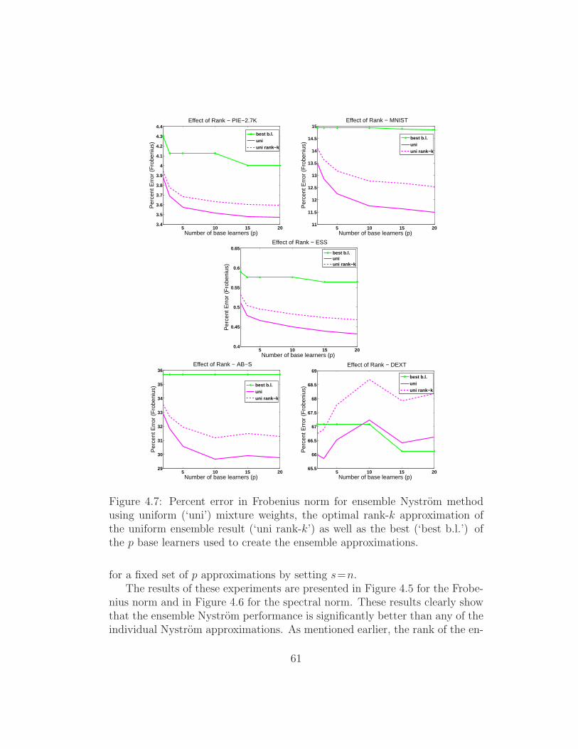
5 10 15 203.4
3.5
3.6
3.7
3.8
3.9
4
4.1
4.2
4.3
4.4
Number of base learners (p)
Per
cent
Err
or (
Fro
beni
us)
Effect of Rank − PIE−2.7K
best b.l.uniuni rank−k
5 10 15 2011
11.5
12
12.5
13
13.5
14
14.5
15
Number of base learners (p)
Per
cent
Err
or (
Fro
beni
us)
Effect of Rank − MNIST
best b.l.uniuni rank−k
5 10 15 200.4
0.45
0.5
0.55
0.6
0.65
Number of base learners (p)
Per
cent
Err
or (
Fro
beni
us)
Effect of Rank − ESS
best b.l.uniuni rank−k
5 10 15 2029
30
31
32
33
34
35
36
Number of base learners (p)
Per
cent
Err
or (
Fro
beni
us)
Effect of Rank − AB−S
best b.l.uniuni rank−k
5 10 15 2065.5
66
66.5
67
67.5
68
68.5
69
Number of base learners (p)
Per
cent
Err
or (
Fro
beni
us)
Effect of Rank − DEXT
best b.l.uniuni rank−k
Figure 4.7: Percent error in Frobenius norm for ensemble Nystrom methodusing uniform (‘uni’) mixture weights, the optimal rank-k approximation ofthe uniform ensemble result (‘uni rank-k’) as well as the best (‘best b.l.’) ofthe p base learners used to create the ensemble approximations.
for a fixed set of p approximations by setting s=n.The results of these experiments are presented in Figure 4.5 for the Frobe-
nius norm and in Figure 4.6 for the spectral norm. These results clearly showthat the ensemble Nystrom performance is significantly better than any of theindividual Nystrom approximations. As mentioned earlier, the rank of the en-
61

5 10 15 20 25
3.35
3.4
3.45
3.5
Relative size of validation set
Per
cent
Err
or (
Fro
beni
us)
Effect of Ridge − PIE−2.7K
no−ridgeridgeoptimal
5 10 15 20 2510.495
10.5
10.505
10.51
10.515
10.52
10.525
Relative size of validation set
Per
cent
Err
or (
Fro
beni
us)
Effect of Ridge − MNIST
no−ridgeridgeoptimal
0 5 10 15 20 25
0.445
0.45
0.455
Relative size of validation set
Per
cent
Err
or (
Fro
beni
us)
Effect of Ridge − ESS
no−ridgeridgeoptimal
0 5 10 15 20 25
26
26.5
27
27.5
28
28.5
Relative size of validation set
Per
cent
Err
or (
Fro
beni
us)
Effect of Ridge − AB−S
no−ridgeridgeoptimal
5 10 15 20 2554.5
55
55.5
56
Relative size of validation set
Per
cent
Err
or (
Fro
beni
us)
Effect of Ridge − DEXT
no−ridgeridgeoptimal
Figure 4.8: Comparison of percent error in Frobenius norm for the ensembleNystrom method with p= 10 experts with weights derived from linear (‘no-ridge’) and ridge (‘ridge’) regression. The dotted line indicates the optimalcombination. The relative size of the validation set equals s/n×100.
semble approximations can be p times greater than the rank of each of the baselearners. Hence, to validate the results in Figures 4.5 and 4.6, we performeda simple experiment in which we compared the performance of the best baselearner to the best rank k approximation of the uniform ensemble approxima-tion (obtained via SVD of the uniform ensemble approximation). The results
62

of this experiment, presented in Figure 4.7, suggest that the performance gainof the ensemble methods is not due to this increased rank.
Furthermore, the ridge regression technique is the best of the proposedtechniques and generates nearly the optimal solution in terms of the percenterror in Frobenius norm. We also observed that when s is increased to approx-imately 5% to 10% of n, linear regression without any regularization performsabout as well as ridge regression for both the Frobenius and spectral norm.Figure 4.8 shows this comparison between linear regression and ridge regres-sion for varying values of s using a fixed number of experts (p=10). Finallywe note that the ensemble Nystrom method tends to converge very quickly,and the most significant gain in performance occurs as p increases from 2 to10.
Large-scale experiments
We now present an empirical study of the effectiveness of the ensemble Nystrommethod on the SIFT-1M dataset in Table 2.1 containing 1 million data points.As is common practice with large-scale datasets, we worked on a cluster of sev-eral machines for this dataset. We present results comparing the performanceof the ensemble Nystrom method, using both uniform and ridge regression mix-ture weights, with that of the best and mean performance across the p Nystromapproximations used to construct Kens. We also make comparisons with theK-means adaptive sampling technique introduced in Section 4.2 (Zhang et al.,2008; Zhang & Kwok, 2009). Although the K-means technique is quite ef-fective at generating informative columns by exploiting the data distribution,the cost of performing K-means becomes expensive for even moderately sizeddatasets, making it difficult to use in large-scale settings. Nevertheless, in thiswork, we include the K-means method in our comparison, and we present re-sults for various subsamples of the SIFT-1M dataset, with n ranging from 5Kto 1M.
To fairly compare these techniques, we performed ‘fixed-time’ experiments.We first searched for an appropriate l such that the percent error for theensemble Nystrom method with ridge weights was approximately 10%, andmeasured the time required by the cluster to construct this approximation.We then allotted an equal amount of time (within 1 second) for the othertechniques, and measured the quality of the resulting approximations. Forthese experiments, we set k = 50 and p = 10, based on the results from theprevious section. Furthermore, in order to speed up computation on this large
63
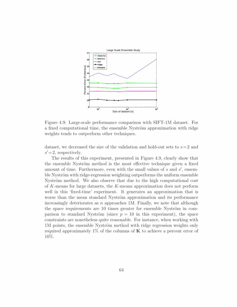
104
105
106
9
10
11
12
13
14
15
16
17
Size of dataset (n)
Per
cent
Err
or (
Fro
beni
us)
Large Scale Ensemble Study
mean b.l.best b.l.uniridgekmeans
Figure 4.9: Large-scale performance comparison with SIFT-1M dataset. Fora fixed computational time, the ensemble Nystrom approximation with ridgeweights tends to outperform other techniques.
dataset, we decreased the size of the validation and hold-out sets to s=2 ands′=2, respectively.
The results of this experiment, presented in Figure 4.9, clearly show thatthe ensemble Nystrom method is the most effective technique given a fixedamount of time. Furthermore, even with the small values of s and s′, ensem-ble Nystrom with ridge-regression weighting outperforms the uniform ensembleNystrom method. We also observe that due to the high computational costof K-means for large datasets, the K-means approximation does not performwell in this ‘fixed-time’ experiment. It generates an approximation that isworse than the mean standard Nystrom approximation and its performanceincreasingly deteriorates as n approaches 1M. Finally, we note that althoughthe space requirements are 10 times greater for ensemble Nystrom in com-parison to standard Nystrom (since p = 10 in this experiment), the spaceconstraints are nonetheless quite reasonable. For instance, when working with1M points, the ensemble Nystrom method with ridge regression weights onlyrequired approximately 1% of the columns of K to achieve a percent error of10%.
64

4.4 Summary
A key aspect to sampling-based matrix approximations is the manner in whichwe choose a subset of representative columns. In this chapter we have discussedboth fixed and adaptive approaches to sampling columns of a matrix. We haveseen that the approximation performance is significantly affected by the choiceof sampling algorithm, and furthermore, that there is often a tradeoff betweenchoosing a more informative set of columns and the efficiency of the samplingalgorithm. Finally, we discussed an ensemble meta-algorithm for combiningmultiple matrix approximations that generates favorable matrix reconstruc-tions and yet naturally fits within a distributed computing environment, thusmaking it quite efficient even in large-scale settings.
65

Chapter 5
Theoretical Analysis
The effectiveness of the Nystrom method hinges on two key assumptions onthe input matrix, K. First, we assume that a low-rank approximation to Kcan be effective for the task at hand. This assumption is often true empiri-cally as demonstrated by the widespread use of Singular Value Decomposition(SVD) and Principal Component Analysis (PCA) in practical applications. Asexpected, the Nystrom method is not appropriate in cases where this assump-tion does not hold, which explains its poor performance in the experimentalresults of Fergus et al. (2009). In Section 5.1, we present theoretical resultsbased on work in Kumar et al. (2009c) and Kumar et al. (2009a) that in-corporate this low-rank assumption by comparing the quality of the Nystromapproximation to the ‘best’ low-rank approximation, i.e., the approximationconstructed from the top singular values and singular vectors of K. This work,related to work by Drineas and Mahoney (2005), provides performance boundsfor the Nystrom method as it is used in practice, i.e., using uniform samplingwithout replacement, and holds for both the standard Nystrom method as wellas the ensemble Nystrom method discussed in Section 4.3.
The second crucial assumption involves the sampling-based nature of thealgorithm, namely that an accurate low-rank approximation can be generatedexclusively from information extracted from a small subset of l ≪ n columnsof K. This assumption is not generally true for all matrices. For instance,consider the extreme case of the n× n matrix described below:
K =
∣∣∣∣∣∣
∣∣∣∣∣∣
e1 . . . er 0 . . . 0∣∣∣∣∣∣
∣∣∣∣∣∣
, (5.1)
66

where ei is the ith column of the n dimensional identity matrix and 0 is then dimensional zero vector. Although this matrix has rank r, it nonethelesscannot be well approximated by a random subset of l columns unless thissubset includes e1, . . . , er. In order to account for such pathological cases, pre-vious theoretical bounds relied on sampling columns of K from a non-uniformdistribution weighted precisely by the magnitude of the diagonal elements ofK, as discussed in Section 4.1. Indeed, these bounds give better guaranteesfor pathological cases. However, in practice, when working with real-worlddatasets, uniform sampling is more commonly used, e.g., Williams and Seeger(2000); Fowlkes et al. (2004); Platt (2004); Talwalkar et al. (2008), since di-agonal sampling is more expensive and does not typically outperform uniformsampling, as discussed in Section 4.1. Hence the diagonal sampling bounds arenot applicable in this setting. Furthermore, these bounds are typically loosefor matrices in which the diagonal entries of the matrix are roughly of the samemagnitude, as in the case of all kernel matrices generated from RBF kernels,for which the Nystrom has been noted to work particularly well (Williams &Seeger, 2000). Adaptive techniques have also been proposed to handle thesepathological cases, though they are not well studied theoretically and in prac-tice are outperformed by uniform sampling given fixed time constraints, asshown in empirical studies in Zhang et al. (2008) and discussed in Section 4.2.
Hence, we propose to characterize the ability to extract information from asmall subset of l columns using the notion of matrix coherence, an alternativedata-dependent measurement which we believe to be intrinsically related tothe algorithm’s performance. Recent work on compressed sensing and matrixcompletion, which also involve sampling-based approximations, have reliedheavily on coherence assumptions (Donoho, 2006; Candes et al., 2006; Candes& Romberg, 2007). Coherence measures the extent to which the singularvectors of a matrix are correlated with the standard basis. Intuitively, if wework with sufficiently incoherent matrices, then we avoid pathological casessuch as the one presented in (5.1), as we will show theoretically and empiricallyin Section 5.2. This research based on work in Talwalkar and Rostamizadeh(2010).
Finally, in Section 5.3, we address the question of how kernel approxima-tion affects the performance of learning algorithms. There exists some previouswork on this subject. Spectral clustering with perturbed data was studied in arestrictive setting with several assumption by Huang et al. (2008). In Fine andScheinberg (2002), the authors address this question in terms of the impact onthe value of the objective function to be optimized by the learning algorithm.
67
However, we strive to take the question one step further and directly analyzethe effect of an approximation in the kernel matrix on the hypothesis generatedby several widely used kernel-based learning algorithms. Based on initial workin Cortes et al. (2010), we give stability bounds based on the norm of thekernel approximation for these algorithms, including SVMs, SVR, KRR, Ker-nel PCA and graph Laplacian-based regularization algorithms (Belkin et al.,2004). These bounds help determine the degree of approximation that canbe tolerated in the estimation of the kernel matrix. Our analysis differs fromprevious applications of stability analysis as put forward by Bousquet andElisseeff (2001). Instead of studying the effect of changing one training point,we study the effect of changing the kernel matrix. Our analysis is generaland applies to arbitrary approximations of the kernel matrix. However, wealso give a specific analysis of the Nystrom low-rank approximation given therecent interest in this method and the successful applications of this algorithmto large-scale applications. We also discuss experimental results for KernelRidge Regression that support our theoretical analyses.
5.1 Nystrom Analysis
We now present a theoretical analysis of the Nystrom method based on workfrom Kumar et al. (2009a) for which we use as tools some results previouslyshown by Drineas and Mahoney (2005) and Kumar et al. (2009c). As inKumar et al. (2009c), we shall use the following generalization of McDiarmid’sconcentration bound to sampling without replacement (Cortes et al., 2008).
Theorem 5.1 Let Z1, . . . , Zl be a sequence of random variables sampled uni-formly without replacement from a fixed set of l+u elements Z, and let φ : Z l→R be a symmetric function such that for all i∈ [1, l] and for all z1, . . . , zl ∈Zand z′1, . . . , z
′l ∈Z, |φ(z1, . . . , zl)−φ(z1, . . . , zi−1, z
′i, zi+1, . . . , zl)|≤ c. Then, for
all ǫ>0, the following inequality holds:
Pr[φ− E[φ] ≥ ǫ
]≤ exp
[ −2ǫ2
α(l,u)c2
], (5.2)
where α(l, u) = lul+u−1/2
11−1/(2 max{l,u}) .
We define the selection matrix corresponding to a sample of l columns asthe matrix S∈R
n×l defined by Sii =1 if the ith column of K is among thosesampled, Sij =0 otherwise. Thus, C=KS is the matrix formed by the columns
68

sampled. Since K is SPSD, there exists X ∈ RN×n such that K = X⊤X. We
shall denote by Kmax the maximum diagonal entry of K, Kmax =maxi Kii, andby dK
max the distance maxij
√Kii + Kjj − 2Kij.
5.1.1 Standard Nystrom method
The following theorem gives an upper bound on the norm-2 error of theNystrom approximation of the form ‖K − K‖2/‖K‖2 ≤ ‖K −Kk‖2/‖K‖2 +O(1/
√l) and an upper bound on the Frobenius error of the Nystrom approx-
imation of the form ‖K− K‖F/‖K‖F ≤ ‖K−Kk‖F/‖K‖F +O(1/l1
4 ).
Theorem 5.2 Let K denote the rank-k Nystrom approximation of K basedon l columns sampled uniformly at random without replacement from K, andKk the best rank-k approximation of K. Then, with probability at least 1− δ,the following inequalities hold for any sample of size l:
‖K− K‖2 ≤ ‖K−Kk‖2 + 2n√lKmax
[1 +
√n−l
n−1/21
β(l,n)log 1
δdK
max/K1
2
max
]
‖K− K‖F ≤ ‖K−Kk‖F +
[64kl
] 1
4nKmax
[1 +
√n−l
n−1/21
β(l,n)log 1
δdK
max/K1
2
max
] 1
2
,
where β(l, n) = 1− 12 max{l,n−l} .
Proof. To bound the norm-2 error of the Nystrom method in the scenario ofsampling without replacement, we start with the following general inequalitygiven by Drineas and Mahoney (2005)[proof of Lemma 4]:
‖K− K‖2 ≤ ‖K−Kk‖2 + 2‖XX⊤ − ZZ⊤‖2, (5.3)
where Z =√
nlXS. We then apply the McDiarmid-type inequality of Theo-
rem 5.1 to φ(S)= ‖XX⊤−ZZ⊤‖2. Let S′ be a sampling matrix selecting thesame columns as S except for one, and let Z′ denote
√nlXS′. Let z and z′
denote the only differing columns of Z and Z′, then
|φ(S′)− φ(S)| ≤ ‖z′z′⊤ − zz⊤‖2 = ‖(z′ − z)z′⊤ + z(z′ − z)⊤‖2 (5.4)
≤ 2‖z′ − z‖2 max{‖z‖2, ‖z′‖2}. (5.5)
Columns of Z are those of X scaled by√n/l. The norm of the difference of
two columns of X can be viewed as the norm of the difference of two feature
69

vectors associated to K and thus can be bounded by dK. Similarly, the norm
of a single column of X is bounded by K1
2
max. This leads to the followinginequality:
|φ(S′)− φ(S)| ≤ 2n
ldK
maxK1
2
max. (5.6)
The expectation of φ can be bounded as follows:
E[Φ] = E[‖XX⊤ − ZZ⊤‖2] ≤ E[‖XX⊤ − ZZ⊤‖F ] ≤ n√lKmax, (5.7)
where the last inequality follows Corollary 2 of Kumar et al. (2009c). Theinequalities (5.6) and (5.7) combined with Theorem 5.1 give a bound on‖XX⊤ − ZZ⊤‖2 and yield the statement of the theorem.
The following general inequality holds for the Frobenius error of the Nystrommethod (Drineas & Mahoney, 2005):
‖K− K‖2F ≤ ‖K−Kk‖2F +√
64k ‖XX⊤ − ZZ⊤‖2F nKmaxii . (5.8)
Bounding the term ‖XX⊤−ZZ⊤‖2F as in the norm-2 case and using the con-centration bound of Theorem 5.1 yields the result of the theorem. 2
5.1.2 Ensemble Nystrom method
The following error bounds hold for ensemble Nystrom methods based on aconvex combination of Nystrom approximations.
Theorem 5.3 Let S be a sample of pl columns drawn uniformly at ran-dom without replacement from K, decomposed into p subsamples of size l,S1, . . . , Sp. For r∈ [1, p], let Kr denote the rank-k Nystrom approximation ofK based on the sample Sr, and let Kk denote the best rank-k approximation ofK. Then, with probability at least 1− δ, the following inequalities hold for anysample S of size pl and for any µ in the simplex ∆ and Kens =
∑pr=1 µrKr:
‖K− Kens‖2 ≤ ‖K−Kk‖2 +
2n√lKmax
[1 + µmaxp
1
2
√n−pl
n−1/21
β(pl,n)log 1
δdK
max/K1
2
max
]
‖K− Kens‖F ≤ ‖K−Kk‖F +
[64kl
] 1
4nKmax
[1 + µmaxp
1
2
√n−pl
n−1/21
β(pl,n)log 1
δdK
max/K1
2
max
] 1
2
,
where β(pl, n) = 1− 12 max{pl,n−pl} and µmax = maxp
r=1 µr.
70

Proof. For r ∈ [1, p], let Zr =√n/lXSr, where Sr denotes the selection
matrix corresponding to the sample Sr. By definition of Kens and the upperbound on ‖K − Kr‖2 already used in the proof of theorem 5.2, the followingholds:
‖K− Kens‖2 =∥∥∥
p∑
r=1
µr(K− Kr)∥∥∥
2≤
p∑
r=1
µr‖K− Kr‖2 (5.9)
≤p∑
r=1
µr
(‖K−Kk‖2 + 2‖XX⊤ − ZrZ
⊤r ‖2
)(5.10)
= ‖K−Kk‖2 + 2
p∑
r=1
µr‖XX⊤ − ZrZ⊤r ‖2. (5.11)
We apply Theorem 5.1 to φ(S)=∑p
r=1 µr‖XX⊤−ZrZ⊤r ‖2. Let S ′ be a sample
differing from S by only one column. Observe that changing one column of thefull sample S changes only one subsample Sr and thus only one term µr‖XX⊤−ZrZ
⊤r ‖2. Thus, in view of the bound (5.6) on the change to ‖XX⊤ −ZrZ
⊤r ‖2,
the following holds:
|φ(S ′)− φ(S)| ≤ 2n
lµmaxd
K
maxK1
2
max, (5.12)
The expectation of Φ can be straightforwardly bounded by:
E[Φ(S)] =
p∑
r=1
µr E[‖XX⊤ − ZrZ⊤r ‖2] ≤
p∑
r=1
µrn√lKmax =
n√lKmax
using the bound (5.7) for a single expert. Plugging in this upper bound andthe Lipschitz bound (5.12) in Theorem 5.1 yields our norm-2 bound for theensemble Nystrom method.
71

For the Frobenius error bound, using the convexity of the Frobenius normsquare ‖·‖2F and the general inequality (5.8), we can write
‖K− Kens‖2F =∥∥∥
p∑
r=1
µr(K− Kr)∥∥∥
2
F≤
p∑
r=1
µr‖K− Kr‖2F (5.13)
≤p∑
r=1
µr
[‖K−Kk‖2F +
√64k ‖XX⊤ − ZrZ
⊤r ‖F nKmax
ii
].
(5.14)
= ‖K−Kk‖2F +√
64k
p∑
r=1
µr‖XX⊤ − ZrZ⊤r ‖F nKmax
ii . (5.15)
The result follows by the application of Theorem 5.1 to ψ(S)=∑p
r=1 µr‖XX⊤−ZrZ
⊤r ‖F in a way similar to the norm-2 case. 2
The bounds of Theorem 5.3 are similar in form to those of Theorem 5.2.However, the bounds for the ensemble Nystrom are tighter than those for anyNystrom expert based on a single sample of size l even for a uniform weighting.In particular, for µi = 1/p for all i, the last term of the ensemble bound for
norm-2 is smaller by a factor larger than µmaxp1
2 = 1/√p.
5.2 Coherence-based Bounds
The main contribution of this section is the connection made between matrixcoherence and the Nystrom method. Making use of related work in the com-pressed sensing and the matrix completion literature, we give a more refinedanalysis of the Nystrom method as a function of matrix coherence. We alsopresent extensive empirical results that strongly relate coherence to the per-formance of the Nystrom method. The results in this section are based onwork from Talwalkar and Rostamizadeh (2010).
5.2.1 Coherence
Although the Nystrom method tends to work well in practice, the performanceof this algorithm depends on the structure of the underlying matrix. We willshow that the performance is related to the size of the entries of the singularvectors of K, or the coherence of its singular vectors. We define Ur as the top
72

r singular vectors of K, and denote the coherence of these singular vectors asµ(Ur), which is adapted from Candes and Romberg (2007).
Definition 5.1 (Coherence) The coherence of a matrix Ur with orthonor-mal columns is defined as:
µ(Ur) =√nmax
i,j|Ur
(j)(i) | . (5.16)
The coherence of Ur is lower bounded by 1, as is the case for the rank-1matrix with all entries equal to 1/
√n, and upper bounded by
√n, as is the
case for the matrix of canonical basis vectors. As discussed in Candes andRecht (2009); Candes and Tao (2009), highly coherent matrices are difficultto randomly recover via matrix completion algorithms, and this same logicextends to the Nystrom method. In contrast, incoherent matrices are mucheasier to successfully complete and to approximate via the Nystrom method,as discussed in Section 5.2.2.
In order to provide some intuition, Candes and Recht (2009) give severalclasses of randomly generated matrices with low coherence. One such class ofmatrices is generated from uniform random orthonormal singular vectors andarbitrary singular values. For such a class they show that µ = O(
√log n 4
√r)
with high probability.1 In what follows, we will show bounds on the numberof points needed for reconstruction that become more favorable as coherencedecreases. However, the bounds are useful for more generous values of coher-ence than given in the above example. We will also provide an empirical studyof coherence for various real-world and synthetic examples.
5.2.2 Low-rank, low-coherence bounds
In this section, we make use of coherence to analyze the Nystrom methodwhen used with low-rank matrices. We note that although the bounds pre-sented throughout this section hold for matrices of any rank r, they are onlyinteresting when r = o(
√n), and hence they are most applicable in the “low-
rank” setting.As discussed in Section 2.2, the Nystrom method generates high quality
low-rank approximations in cases where K has low-rank structure even if the
1For low-rank matrices, 4√
r is quite small. Moreover, this 4√
r factor only appears due toour use of the generally loose inequality µ2 ≤ √rµ1, where µ1 is a slightly different notion ofcoherence used in the original bound in Candes and Recht (2009) for this class of matrices.
73

matrix has full rank, i.e., K ≈ Kk for some k ≪ n. Furthermore, as statedin Theorem 2.3, when K is actually a low-rank matrix, then the Nystrommethod can exactly recover the initial matrix. This theorem implies that if Khas low-rank and l ≥ k ≥ r, then there exists a particular sampling such thatrank(W) = rank(K) and the Nystrom method can perfectly recover the fullmatrix. However, selecting a suitable set of l columns from an n × n SPSDmatrix can be an intractable combinatorial problem, and there exist matricesfor which the probability of selecting such a subset uniformly at random isexponentially small, e.g., the rank-r SPSD diagonal matrices discussed earlier.In contrast, a large class of SPSD matrices are much more incoherent, andfor these matrices, we will next show that by choosing l to be linear in r andlogarithmic in n we can with very high probability guarantee that rank(W) =r, and hence exactly recover the initial matrix.
Probability of choosing a good subset
We start with a rank-r Gram matrix, K, and a fixed distribution, D, over thecolumns of K. Our goal is to calculate the probability of randomly choosing asubset of l columns of K according to D such that rank(W) = r. Recall thatK = X⊤X, X = [X1 X2] and W = X⊤
1 X1. Then, by properties of SVD,we know that rank(K) = rank(X) and rank(W) = rank(X1). Hence, theprobability of this desired event is equivalent to the probability of samplingl columns of X according to D such that rank(X1) = r, as shown in (5.18).Next, we can write the thin SVD of X as X = UXΣXV⊤
X , where UX ∈R
N×r, ΣX ∈ Rr×r and VX ∈ R
n×r. Since UX contains orthonormal columnsand ΣX is invertible, we know that Σ−1
X U⊤XX = V⊤
X . Further, using the blockrepresentation of X, we have
X⊤1 UXΣ−1
X = VX (1:l), (5.17)
where VX (1:l) ∈ Rl×r corresponds to the first l rows of VX , i.e., the first
l components for each of the r right singular vectors of X. Since the leftsingular vectors of X span the columns X and hence of X1, we know thatrank(X1) = rank(X⊤
1 UXΣ−1X ) and we obtain the equality of (5.19).
PrD
[rank(W) = r] = PrD
[rank(X1) = r] (5.18)
= PrD
[rank(VX (1:l)) = r]. (5.19)
In the next section we calculate this probability for a specific distribution interms of l as well as a measure of the coherence of VX .
74

Dataset Type of data # Points (n) # Features (d) KernelPIE face images 2731 2304 linearMNIST digit images 4000 784 linearEssential proteins 4728 16 RBFAbalone abalones 4177 8 RBFDexter bag of words 2000 20000 linearArtificial random features 1000 20000 linear
Table 5.1: Description of the datasets used in our coherence experiments,including the type of data, the number of points (n), the number of features(d) and the choice of kernel (Sim et al., 2002; LeCun & Cortes, 1998; Gustafsonet al., 2006; Asuncion & Newman, 2007).
Sampling bound
Given the orthonormal matrix Ur, we would like to find a choice of l suchthat VX (1:l) created by uniform sampling has rank r with high probability. Aspointed out in the previous section, a meaningful bound may not be possiblefor any l < n if no assumption is made on Vr. Here we adopt the assumptionthat Vr has low coherence, as defined in Definition 5.1. If we define A =VX
⊤(1:l)VX (1:l), we then observe that by properties of SVD we have
Pr(rank(VX (1:l)) = r
)= Pr
(rank(A) = r
). (5.20)
Next, we define σ = ‖A‖2 and note that for 0 < c < 1/σ, cA is an r × rSPSD matrix with singular values less than one. Furthermore, I− cA is alsoSPSD with
Pr(rank(A) = r
)= Pr
(‖cA− I‖2 < 1
), (5.21)
since ‖cA− I‖ = 1 implies that the nullspace of A is nonempty. Alternatively,if c ≥ 1/σ, then
Pr(rank(A) = r
)≥ Pr
(‖cA− I‖2 < 1
), (5.22)
since, for large enough c, we could have ‖cA − I‖2 ≥ 1 even if rank(A) = r.Thus the inequality in (5.22) holds for any constant c > 0, i.e., the probabilityon the RHS of (5.22) serves as a lower bound to the probability of interest.
The probability on the RHS of (5.22) has been studied in previous com-pressive sampling literature. Specifically, Candes and Romberg (2007) makes
75

use of a main lemma of Rudelson (1999) to derive Theorem 5.4, which providesus with our desired lower bound.
Theorem 5.4 ((Candes & Romberg, 2007) Thm 1.2) Define V ∈ Rn×r
such that V⊤V = I and let V(1:l) ∈ Rl×r be generated from V by sampling l
rows uniformly at random. Then, the following holds with probability at least1− δ,
∥∥nlV⊤
(1:l)V(1:l) − I∥∥ < 1
2, (5.23)
for any l that satisfies,
l ≥ rµ2(V) max(C1 log(r), C2 log(3/δ)
), (5.24)
where C1 and C2 are positive constants.
Note that our definition of coherence and statement of Theorem 5.4 aremodified to account for the fact that V⊤V = I as oppose to nI, as in Candesand Romberg (2007). Also, V is not square as assumed in the original theorem,however it can be verified that the proof holds even for this case.
By making use of Theorem 5.4, we can now answer the question regardingthe number of columns needed to sample from K in order to obtain an exactreconstruction via the Nystrom method. Theorem 5.5 presents a bound on lfor matrix completion in terms of µ.
Theorem 5.5 Let K = UΣU⊤ ∈ Rn×n be a rank-r SPSD matrix, where
(Σ, U) are matrices of its singular values and singular vectors. Then it sufficesto sample l ≥ rµ2(V) max
(C1 log(r), C2 log(3/δ)
)columns, where C1 and C2
are positive constants, to have with probability at least 1− δ,
‖K− Kk‖ = 0 . (5.25)
Proof. Theorem 2.3 states sufficient conditions for exact matrix completion.Equations (5.18) and (5.19) reduce these sufficient conditions to a condition onthe rank of VX (1:l). Equations (5.20) and (5.22) further reduce this problemto a similar problem previously studied in the context of compressed sensing.Finally, we use Theorem 5.4 to bound with high probability the RHS of (5.22).2
76

5.2.3 Experiments
In this section we present a series of empirical results that show the empiricalconnection between matrix coherence and the performance of the Nystrommethod. We first perform experiments that corroborate the theoretical claimsmade in the previous section. We work with the six datasets detailed in Table5.1 to illustrate the performance of the Nystrom method for low-rank matri-ces, and then interpret these results in the context of the coherence of thesedatasets. We then present more general experimental results that connectmatrix coherence to the Nystrom method in the case of full rank matrices.
0 50 100 150 2000
0.1
0.2
0.3
0.4
0.5
0.6
0.7
0.8
0.9
Number of Sampled Columns (l)
Per
cent
Err
or
Reconstruction Error
AbaloneDexterEssentialMNISTPIEArtificial
50 60 70 80 90 100 110 120 1300
0.05
0.1
0.15
0.2
Number of Sampled Columns (l)
Per
cent
Err
or
Reconstruction Error
AbaloneDexterEssentialMNISTPIEArtificial
Figure 5.1: Mean percent error over 10 trials of Nystrom approximations ofrank 100 matrices. Left: Results for l ranging from 5 to 200. Right: Detailedview of experimental results for l ranging from 50 to 130.
Reconstruction
In our first set of experiments we measure the accuracy of the Nystrom ap-proximation (Kk) for a variety of rank-r matrices, with r = 100. For each ofthe six datasets listed above, we first constructed the optimal rank-r approxi-mation to each kernel matrix by reconstructing with the top r singular valuesand singular vectors. Next, we performed the Nystrom method for variousvalues of l to generate a series of approximations to our rank-r matrix (notethat we set k = l). For each approximation, we calculated the percent error ofthe Nystrom approximation using the notion of percent error, which we have
77

previously defined as follows:
Percent error =‖K− Kk‖F‖K‖F
× 100.
The results of this experiment, averaged over 10 trials, are presented in Figure5.1. The figure shows that for five of the six datasets, the Nystrom methodexactly reconstructs the initial rank r matrix when the number of sampledcolumns (l) is equal or slightly larger than r. Note that this observation holdsfor each of the ten trials, since the mean error is zero for each of these datasetswhen l ≈ r. In contrast, for the case of the Abalone dataset, we do not seeconvergence to zero percent error as l surpasses r, and the percent error isnon-zero even when l = 2r.
1000 1500 2000 2500 3000 3500 4000 4500 50000
5
10
15
20
25
30
35
40
45
50
55
Dataset Size (n)
Coh
eren
ce
Coherence of Datasets
AbaloneDexterEssentialMNISTPIEArtificial
0 1000 2000 3000 4000 50000
5
10
15
20
25
30
35
40
45
50
Dataset Size (n)
Coh
eren
ceAsymptotic Coherence Comparison
AbaloneMNIST
Figure 5.2: Coherence of Datasets. Left: Coherence of rank 100 SPSD ma-trices derived from datasets listed in Table 5.1. Right: Asymptotic growth ofcoherence for MNIST and Abalone datasets. Note that coherence values aremeans over ten trials.
Coherence of datasets
In this set of experiments, we use the concept of coherence to explain theselow-rank reconstruction results, namely that the Nystrom method generatesan exact matrix reconstruction for l ≈ r for five of the six datasets, but failsto do so for the Abalone dataset. As such, we first calculated the coherenceof each of the six SPSD rank 100 matrices used in these experiments, using
78
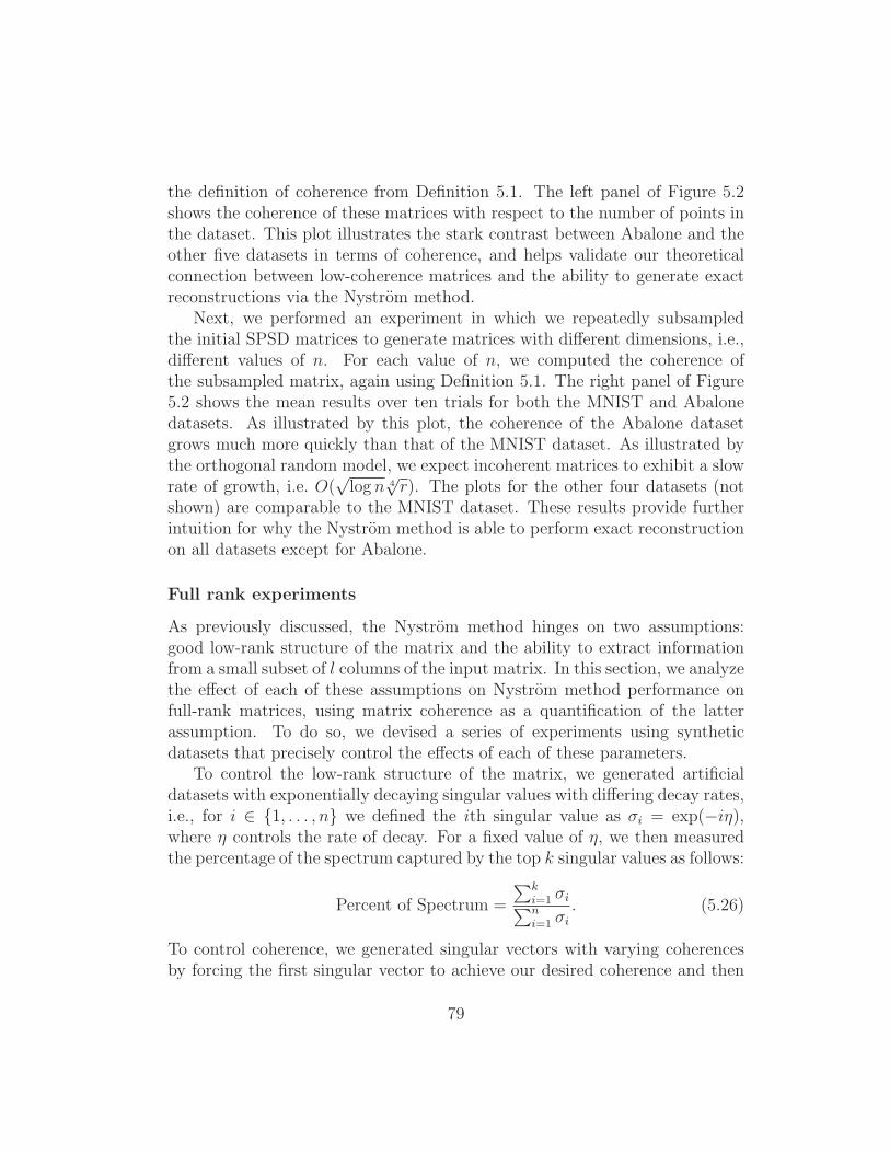
the definition of coherence from Definition 5.1. The left panel of Figure 5.2shows the coherence of these matrices with respect to the number of points inthe dataset. This plot illustrates the stark contrast between Abalone and theother five datasets in terms of coherence, and helps validate our theoreticalconnection between low-coherence matrices and the ability to generate exactreconstructions via the Nystrom method.
Next, we performed an experiment in which we repeatedly subsampledthe initial SPSD matrices to generate matrices with different dimensions, i.e.,different values of n. For each value of n, we computed the coherence ofthe subsampled matrix, again using Definition 5.1. The right panel of Figure5.2 shows the mean results over ten trials for both the MNIST and Abalonedatasets. As illustrated by this plot, the coherence of the Abalone datasetgrows much more quickly than that of the MNIST dataset. As illustrated bythe orthogonal random model, we expect incoherent matrices to exhibit a slowrate of growth, i.e. O(
√log n 4
√r). The plots for the other four datasets (not
shown) are comparable to the MNIST dataset. These results provide furtherintuition for why the Nystrom method is able to perform exact reconstructionon all datasets except for Abalone.
Full rank experiments
As previously discussed, the Nystrom method hinges on two assumptions:good low-rank structure of the matrix and the ability to extract informationfrom a small subset of l columns of the input matrix. In this section, we analyzethe effect of each of these assumptions on Nystrom method performance onfull-rank matrices, using matrix coherence as a quantification of the latterassumption. To do so, we devised a series of experiments using syntheticdatasets that precisely control the effects of each of these parameters.
To control the low-rank structure of the matrix, we generated artificialdatasets with exponentially decaying singular values with differing decay rates,i.e., for i ∈ {1, . . . , n} we defined the ith singular value as σi = exp(−iη),where η controls the rate of decay. For a fixed value of η, we then measuredthe percentage of the spectrum captured by the top k singular values as follows:
Percent of Spectrum =
∑ki=1 σi∑ni=1 σi
. (5.26)
To control coherence, we generated singular vectors with varying coherencesby forcing the first singular vector to achieve our desired coherence and then
79

0 5 10 15 200
0.1
0.2
0.3
0.4
0.5
Percentage of Columns Sampled
Per
cent
Err
orPercent of Spectrum: 80.8%
mu=4.6mu=14.8mu=24.9mu=35.3
0 5 10 15 200
0.1
0.2
0.3
0.4
0.5
Percentage of Columns Sampled
Per
cent
Err
or
Percent of Spectrum: 90.9%
mu=4.6mu=14.8mu=24.9mu=35.3
0 5 10 15 200
0.1
0.2
0.3
0.4
0.5
Percentage of Columns Sampled
Per
cent
Err
or
Percent of Spectrum: 95.0%
mu=4.6mu=14.8mu=24.9mu=35.3
0 5 10 15 200
0.1
0.2
0.3
0.4
0.5
Percentage of Columns Sampled
Per
cent
Err
or
Percent of Spectrum: 99.3%
mu=4.6mu=14.8mu=24.9mu=35.3
Figure 5.3: Coherence experiments with full rank synthetic datasets. Each plotcorresponds to matrices with a fixed singular value decay rate (resulting in afixed percentage of spectrum captured) and each line within a plot correspondsto the average results of 10 randomly generated matrices with the specifiedcoherence.
using QR to generate a full orthogonal basis. The smallest values of µ used inour experiments correspond to randomly generated orthogonal matrices. Wereport the results of our experiments in Figure 5.3. For these experimentswe set n = 2000 and k = 50. Each plot corresponds to matrices with a fixedsingular value decay rate (resulting in a fixed percentage of spectrum captured)and each line within a plot corresponds to the average results of 10 randomlygenerated matrices with the specified coherence. Furthermore, results for eachsuch matrix for a fixed percentage of sampled columns are the means over 5random subsets of columns.
There are two main observations to be drawn from our experiments. First,
80

as noted in previous work with the Nystrom method, the Nystrom methodgenerates better approximations for matrices with better low-rank structure,i.e., matrices with a higher percentage of spectrum captured by the top k sin-gular values. Second, following the same pattern as in the low-rank setting,the Nystrom method generates better approximations for lower coherence ma-trices, and hence, matrix coherence appears to effectively capture the degreeto which information can be extracted from a subset of columns.
5.3 Kernel Stability
Up to this point, we have focused on reconstruction performance while analyz-ing the Nystrom method. In this section we take a different approach, as weanalyze the impact of kernel approximation on several common kernel-basedlearning algorithms: KRR, SVM, SVR, Kernel PCA and graph Laplacian-based regularization algorithms. Our stability analyses result in bounds onthe hypotheses directly in terms of the quality of the kernel approximation.Some of the results in this section are based on work in Cortes et al. (2010).
In our analysis we assume that the kernel approximation is only used duringtraining where the kernel approximation may serve to reduce resource require-ments. At testing time the true kernel function is used. This scenario thatwe are considering is standard for the Nystrom method and other approxima-tions. We consider the standard supervised learning setting where the learningalgorithm receives a sample of n labeled points S = ((x1, y1), . . . , (xn, yn)) ∈(X × Y )n, where X is the input space and Y the set of labels, Y = R with|y| ≤ M in the regression case, and Y = {−1,+1} in the classification case.We will also assume that K′ is a symmetric, positive, and semi-definite (SPSD)approximation of the SPSD kernel matrix K.2 Hence, K and K′ correspond topositive definite symmetric kernel functions K(·, ·) and K ′(·, ·), respectively.
2Note that we are using the notation K′ to indicate an arbitrary SPSD approximation
of K. In contrast, throughout this thesis K has referred to SPSD approximations generatedfrom sampling-based algorithms.
81

5.3.1 Kernel Ridge Regression
We first provide a stability analysis of Kernel Ridge Regression. The followingis the dual optimization problem solved by KRR (Saunders et al., 1998):
maxα∈Rn
λα⊤α + αKα− 2α⊤y, (5.27)
where λ=nλ0>0 is the ridge parameter. The problem admits the closed formsolution α=(K+λI)−1y. We denote by h the hypothesis returned by KernelRidge Regression when using the exact kernel matrix.
Proposition 5.1 Let h′ denote the hypothesis returned by Kernel Ridge Re-gression when using the approximate kernel matrix K′ ∈ R
n×n. Furthermore,define κ > 0 such that K(x, x) ≤ κ and K ′(x, x) ≤ κ for all x ∈ X. Thiscondition is verified with κ = 1 for Gaussian kernels for example. Then thefollowing inequalities hold for all x ∈ X,
|h′(x)− h(x)| ≤ κM
λ20n‖K′ −K‖2. (5.28)
Proof. Let α′ denote the solution obtained using the approximate kernel
matrix K′. We can write
α′ −α = (K′ + λI)−1y − (K + λI)−1y (5.29)
= −[(K′ + λI)−1(K′ −K)(K + λI)−1
]y, (5.30)
where we used the identity M′−1 −M−1 =−M′−1(M′ −M)M−1 valid for anyinvertible matrices M,M′. Thus, ‖α′ −α‖ can be bounded as follows:
‖α′ −α‖ ≤ ‖(K′ + λI)−1‖2‖K′ −K‖2‖(K + λI)−1‖2‖y‖
≤ ‖K′ −K‖2 ‖y‖λmin(K′ + λI)λmin(K + λI)
, (5.31)
where λmin(K′ +λI) is the smallest singular value of K′ +λI and λmin(K+λI)
the smallest singular value of K + λI. The hypothesis h derived with theexact kernel matrix is defined by h(x)=
∑ni=1 αiK(x, xi)=α
⊤kx, where kx =(K(x, x1), . . . , K(x, xn))⊤. By assumption, no approximation affects kx, thusthe approximate hypothesis h′ is given by h′(x)=α
′⊤kx and
|h′(x)− h(x)| ≤ ‖α′ −α‖‖kx‖ ≤ κ√n‖α′ −α‖. (5.32)
82

Using the bound on ‖α′−α‖ given by inequality (5.31), the fact that thesingular values of (K′ + λI) and (K + λI) are larger than or equal to λ sinceK and K′ are SPSD matrices, and ‖y‖≤√nM yields
|h′(x)− h(x)| ≤ κnM‖K′ −K‖2λmin(K′ + λI)λmin(K + λI)
≤ κM
λ20n‖K′ −K‖2.
2
The generalization bounds for KRR, e.g., stability bounds (Bousquet & Elis-
seeff, 2001), are of the form R(h) ≤ R(h)+O(1/√n), where R(h) denotes
the generalization error and R(h) the empirical error of a hypothesis h withrespect to the square loss. The proposition shows that |h′(x) − h(x)|2 =O(‖K′−K‖22/λ4
0n2). Thus, it suggests that the kernel approximation toler-
ated should be such that ‖K′−K‖22/λ40n
2 ≪ O(1/√n), that is, such that
‖K′−K‖2≪O(λ20n
3/4).Note that the main bound used in the proof of the theorem, inequality
(5.31), is tight in the sense that it can be matched for some kernels K andK ′. Indeed, let K and K ′ be the kernel functions defined by K(x, y)=β andK ′(x, y) =β′ if x= y, K ′(x, y) = K(x, y) = 0 otherwise, with β, β′≥ 0. Then,the corresponding kernel matrices for a sample S are K=βI and K′=β′I, andthe dual parameter vectors are given by α=y/(β+λ) and α
′=y/(β′+λ). Now,since λmin(K
′ + λI)=β′+λ and λmin(K + λI)=β+λ, and ‖K′ −K‖=β′ − β,the following equality holds:
‖α′ −α‖ =|β′ − β|
(β′ + λ)(β + λ)‖y‖ (5.33)
=‖K′ −K‖
λmin(K′ + λI)λmin(K′ + λI)‖y‖. (5.34)
This limits significant improvements of the bound of Proposition 5.1 usingsimilar techniques.
5.3.2 Support Vector Machines
This section analyzes the kernel stability of SVMs. For simplicity, we shallconsider the case where the classification function sought has no offset. In
83

practice, this corresponds to using a constant feature. Let Φ: X → F denotea feature mapping from the input space X to a Hilbert space F correspondingto some kernel K. The hypothesis set we consider is thus H = {h : ∃w ∈F |∀x ∈ X, h(x)=w⊤Φ(x)}.
The following is the standard primal optimization problem for SVMs:
minw
FK(w) =1
2‖w‖2 + C0RK(w), (5.35)
where RK(w)= 1n
∑ni=1 L(yiw
⊤Φ(xi)) is the empirical error and L(yiw⊤Φ(xi))=
max(0, 1− yiw⊤Φ(xi)) is the hinge loss associated to the ith point.
In the following, we analyze the difference between the hypothesis h re-turned by SVMs when trained on the sample S of n points and using a kernelK, versus the hypothesis h′ obtained when training on the same sample withthe kernel K ′. For a fixed x ∈ X, we shall compare more specifically h(x) andh′(x). Thus, we can work with the finite set Xn+1 = {x1, . . . , xn, xn+1}, withxn+1 =x.
Different feature mappings Φ can be associated to the same kernel K. Tocompare the solutions w and w′ of the optimization problems based on FK
and FK′ , we can choose the feature mappings Φ and Φ′ associated to K andK ′ such that they both map to R
n+1 as follows. Let Kn+1 denote the Grammatrix associated to K and K′
n+1 that of kernel K ′ for the set of points Xn+1.Then for all u ∈ Xn+1, Φ and Φ′ can be defined by
Φ(u) = K+1/2n+1
K(x1, u)...
K(xn+1, u)
(5.36)
and Φ′(u) = K′+1/2n+1
K ′(x1, u)
...K ′(xn+1, u)
, (5.37)
where K+n+1 denotes the pseudo-inverse of Kn+1 and K′+
n+1 that of K′n+1. It
is not hard to see then that for all u, v ∈ Xn+1, K(u, v) = Φ(u)⊤Φ(v) andK ′(u, v) = Φ′(u)⊤Φ′(v) (Scholkopf & Smola, 2002). Since the optimizationproblem depends only on the sample S, we can use the feature mappings justdefined in the expression of FK and FK′ . This does not affect in any way thestandard SVMs optimization problem.
84
Let w ∈ Rn+1 denote the minimizer of FK and w′ that of FK′ . By defini-
tion, if we let ∆w denote w′ −w, for all s ∈ [0, 1], the following inequalitieshold:
FK(w) ≤ FK(w + s∆w) (5.38)
and FK′(w′) ≤ FK′(w′ − s∆w). (5.39)
Summing these two inequalities, rearranging terms, and using the identity(‖w+s∆w‖2−‖w‖2)+(‖w′−s∆w‖2−‖w′‖2)=−2s(1−s)‖∆w‖2, we obtain asin Bousquet and Elisseeff (2001):
s(1− s)‖∆w‖2 ≤ C0
[(RK(w + s∆w)− RK(w)
)
+(RK′(w′ − s∆w)− RK′(w′)
)].
Note that w + s∆w = sw′ + (1 − s)w and w′ − s∆w = sw + (1 − s)w′.
Then, by the convexity of the hinge loss and thus RK and RK′ , the followinginequalities hold:
RK(w + s∆w)−RK(w)≤s(RK(w′)−RK(w))
RK′(w′−s∆w)−RK′(w′)≤−s(RK′(w′)−RK′(w)).
Plugging in these inequalities on the left-hand side, simplifying by s and takingthe limit s→0 yields
‖∆w‖2 ≤ C0
[(RK(w′)−RK′(w′)
)+
(RK′(w)−RK(w)
)]
=C0
n
n∑
i=1
[(L(yiw
′⊤Φ(xi))− L(yiw′⊤Φ′(xi))
)
+(L(yiw
⊤Φ′(xi))− L(yiw⊤Φ(xi)
)],
where the last inequality results from the definition of the empirical error.Since the hinge loss is 1-Lipschitz, we can bound the terms on the right-hand
85

side as follows:
‖∆w‖2 ≤ C0
n
n∑
i=1
[‖w′‖‖Φ′(xi)− Φ(xi)‖
+ ‖w‖‖Φ′(xi)− Φ(xi)‖]
(5.40)
=C0
n
n∑
i=1
(‖w′‖+ ‖w‖) ‖Φ′(xi)− Φ(xi)‖. (5.41)
Let ei denote the ith unit vector of Rn+1, then (K(x1, xi), . . . , K(xn+1, xi))
⊤=Kn+1ei. Thus, in view of the definition of Φ, for all i ∈ [1, n+ 1],
Φ(xi) = K+1/2n+1 [K(x1, xi), . . . , K(xn, xi), K(x, xi)]
⊤
= K+1/2n+1 Kn+1ei = K
1/2n+1ei, (5.42)
and similarly Φ′(xi)=K′1/2n+1ei. K
1/2n+1ei is the ith column of K
1/2n+1 and similarly
K′1/2ei the ith column of K′1/2n+1. Thus, (5.41) can be rewritten as
‖w′ −w‖2 ≤ C0
n
n∑
i=1
(‖w′‖+ ‖w‖
)‖(K′1/2
n+1 −K1/2n+1)ei‖.
As for the case of KRR, we shall assume that there exists κ > 0 such thatK(x, x)≤ κ and K ′(x, x)≤ κ for all x ∈ Xn+1. Now, since w can be writtenin terms of the dual variables 0≤αi≤C, C=C0/n as w=
∑ni=1 αiK(xi, ·), it
can be bounded as ‖w‖ ≤ nC0/nκ1/2 = κ1/2C0 and similarly ‖w′‖ ≤ κ1/2C0.
Thus, we can write
‖w′ −w‖2 ≤ 2C20κ
1/2
n
n∑
i=1
‖(K′1/2n+1 −K
1/2n+1)ei‖
≤ 2C20κ
1/2
n
n∑
i=1
‖(K′1/2n+1 −K
1/2n+1)‖‖ei‖
= 2C20κ
1/2‖K′1/2n+1 −K
1/2n+1‖. (5.43)
Let K denote the Gram matrix associated to K and K′ that of kernel K ′ forthe sample S. Then, using Lemma 5.1 the following result holds.
86

Lemma 5.1 Let M and M′ be two n×n SPSD matrices. Then, the followingbound holds for the difference of the square root matrices: ‖M′1/2 −M1/2‖2 ≤‖M′ −M‖1/2
2 .
Proof. Since M′−M � ‖M′−M‖2I where I is the n×n identity matrix. Thus,M′�M + ‖M′−M‖2I and M′1/2 � (M + λI)1/2, with λ=‖M′−M‖2. Thus,λmax(M
′) ≤ (λmax(M) + λ)1/2 ≤ λmax(M)1/2 + λ1/2, by sub-additivity of√·.
This shows that λmax(M′)−λmax(M)1/2 ≤ λ and by symmetry λmax(M)1/2−
λmax(M′) ≤ λ1/2, thus ‖M′1/2 −M1/2‖2 ≤ ‖M′ −M‖1/2
2 , which proves thestatement of the lemma. 2
Proposition 5.2 Let h′ denote the hypothesis returned by SVMs when usingthe approximate kernel matrix K′ ∈ R
n×n. Then, the following inequality holdsfor all x ∈ X :
|h′(x)− h(x)| ≤√
2κ3
4C0‖K′ −K‖1
4
2
[1 +
[‖K′−K‖2
4κ
] 1
4
]. (5.44)
Proof. In view of (5.42) and (5.43), the following holds:
|h′(x)− h(x)|= ‖w′⊤Φ′(x)−w⊤Φ(x)‖= ‖(w′ −w)⊤Φ′(x) + w⊤(Φ′(x)− Φ(x))‖≤ ‖w′ −w‖‖Φ′(x)‖+ ‖w‖‖Φ′(x)− Φ(x)‖= ‖w′ −w‖‖Φ′(x)‖+ ‖w‖‖Φ′(xn+1)− Φ(xn+1)‖
≤(2C2
0κ1/2‖K′1/2
n+1 −K1/2n+1‖
)1/2
κ1/2
+ κ1/2C0‖(K′1/2n+1 −K
1/2n+1)en+1‖
≤√
2κ3/4C0‖K′1/2n+1 −K
1/2n+1‖1/2
+ κ1/2C0‖K′1/2n+1 −K
1/2n+1‖.
Now, by Lemma 5.1, ‖K′1/2n+1−K
1/2n+1‖2≤‖K′
n+1−Kn+1‖1/22 . By assumption, the
kernel approximation is only used at training time so K(x, xi)=K ′(x, xi), forall i∈ [1, n], and since by definition x=xn+1, the last rows or the last columnsof the matrices K′
n+1 and Kn+1 coincide. Therefore, the matrix K′n+1−Kn+1
coincides with the matrix K′−K bordered with a zero-column and zero-rowand ‖K′1/2
n+1−K1/2n+1‖2≤‖K′−K‖1/2
2 . Thus,
|h′(x)− h(x)| ≤√
2κ3/4C0‖K′ −K‖1/4 + κ1/2C0‖K′ −K‖1/2, (5.45)
87

which is exactly the statement of the proposition. 2
Since the hinge loss l is 1-Lipschitz, Proposition 5.2 leads directly to thefollowing bound on the pointwise difference of the hinge loss between the hy-potheses h′ and h.
Corollary 5.1 Let h′ denote the hypothesis returned by SVMs when using theapproximate kernel matrix K′ ∈ R
n×n. Then, the following inequality holdsfor all x ∈ X and y ∈ Y:
∣∣L(yh′(x)
)− L
(yh(x)
)∣∣ ≤√
2κ3
4C0‖K′ −K‖1
4
2
[1 +
[‖K′−K‖2
4κ
] 1
4
]. (5.46)
The bounds we obtain for SVMs are weaker than our bound for KRR. Thisis due mainly to the different loss functions defining the optimization problemsof these algorithms.
5.3.3 Support Vector Regression
This section analyzes the kernel stability of Support Vector Regression. Aswith the case of SVMs, we shall consider the case where the regression functionsought has no offset. Let Φ: X → F denote a feature mapping from the inputspace X to a Hilbert space F corresponding to some kernel K. The hypothesisset we consider is thus H = {h : ∃w ∈ F |∀x ∈ X, h(x) = w⊤Φ(x)}. Thestandard primal optimization problem for SVR is identical to that of SVMs asexpressed in (5.35), except that the hinge loss is replaced by the ǫ-insensitiveloss, i.e., L(yi −w⊤Φ(xi))=max(0, |yi −w⊤Φ(xi)| − ǫ).
Our goal is to analyze the difference between the hypothesis h returned bySVR when trained on the sample S of n points and using a kernelK, versus thehypothesis h′ obtained when training on the same sample with the kernel K ′.In the previous section, we presented perturbation bounds for SVMs. However,this analysis is in fact more general, as the proof technique from Section 5.3.2holds for all optimization problems of the form described in (5.35) that useconvex and Lipschitz loss functions. Hence, Corollary 5.2 details the kernelstability bound for SVR that follows directly from the analysis in Section5.3.2 along with the fact that the ǫ-insensitive loss function is convex and1-Lipschitz.
88

Corollary 5.2 Let h′ denote the hypothesis returned by SVR when using theapproximate kernel matrix K′ ∈ R
n×n. Then, the following inequality holdsfor all x ∈ X :
|h′(x)− h(x)| ≤√
2κ3
4C0‖K′ −K‖1
4
2
[1 +
[‖K′−K‖2
4κ
] 1
4
]. (5.47)
5.3.4 Graph Laplacian regularization algorithms
We next study the kernel stability of graph-Laplacian regularization algo-rithms such as that of Belkin et al. (2004). Given a connected weighted graphG= (X,E) in which edge weights can be interpreted as similarities betweenvertices, the task consists of predicting the vertex labels of u vertices using alabeled training sample S of n vertices. The input space X is thus reducedto the set of vertices, and a hypothesis h : X → R can be identified with thefinite-dimensional vector h of its predictions h = [h(x1), . . . , h(xn+u)]
⊤. Thehypothesis set H can thus be identified with R
n+u here. Let hS denote the re-striction of h to the training points, [h(x1), . . . , h(xn)]⊤∈R
n, and similarly letyS denote [y1, . . . , yn]⊤∈R
n. Then, the following is the optimization problemcorresponding to this problem:
minh∈H
h⊤Lh +C0
n(hS − yS)⊤(hS − yS) (5.48)
subject to h⊤1 = 0,
where L is the graph Laplacian and 1 the column vector with all entries equalto 1. Thus, h⊤Lh =
∑nij=1wij(h(xi)− h(xj))
2, for some weight matrix (wij).
The label vector y is assumed to be centered, which implies that 1⊤y = 0.Since the graph is connected, the singular value zero of the Laplacian hasmultiplicity one.
Define IS ∈R(n+u)×(n+u) to be the diagonal matrix with [IS]i,i = 1 if i ≤ n
and 0 otherwise. Maintaining the notation used in Belkin et al. (2004), we letPH denote the projection on the hyperplane H orthogonal to 1 and let M =
PH
(nC0
L + IS
)and M′ = PH
(nC0
L′ + IS
). We denote by h the hypothesis
returned by the algorithm when using the exact kernel matrix L and by L′ anapproximate graph Laplacian such that h⊤L′h =
∑nij=1w
′ij(h(xi) − h(xj))
2,based on matrix (w′
ij) instead of (wij). We shall assume that there exist M>0such that yi≤M for i∈ [1, n].
89

Proposition 5.3 Let h′ denote the hypothesis returned by the graph-Laplacianregularization algorithm when using an approximate Laplacian L′ ∈ R
n×n.Then, the following inequality holds:
‖h′ − h‖ ≤ n3/2M/C0
( nC0
λ2 − 1)2‖L′ − L‖, (5.49)
where λ2 =max{λ2, λ′2} with λ2 denoting the second smallest singular value of
the kernel matrix L and λ′2 the second smallest singular value of L′.
Proof. The closed-form solution of (5.48) is given by Belkin et al. (2004):
h=(PH
(nC0
L+IS
))−1
yS. Thus, we can use that expression and the matrix
identity for (M−1−M′−1) we already used in the analysis of KRR to write
‖h− h′‖ = ‖M−1yS −M′−1yS‖= ‖(M−1 −M′−1)yS‖= ‖−M−1(M−M′)M′−1yS‖≤ n
C0
‖−M−1(L− L′)M′−1yS‖
≤ n
C0
‖M−1‖ ‖M′−1‖ ‖yS‖ ‖L′ − L‖. (5.50)
For any column matrix z ∈R(n+u)×1, by the triangle inequality and the pro-
jection property ‖PHz‖ ≤ ‖z‖, the following inequalities hold:
‖ nC0
PHL‖ = ‖ nC0
PHL + PHISz− PHISz‖
≤ ‖ nC0
PHL + PHISz‖+ ‖PHISz‖
≤ ‖PH
( n
C0
L + IS
)z‖+ ‖ISz‖.
This yields the lower bound:
‖Mz‖ = ‖PH
(n
C0
L + IS
)z‖
≥ n
C0
‖PHL‖ − ‖ISz‖
≥(n
C0
λ2 − 1
)‖z‖,
90

which gives the following upper bounds on ‖M−1‖ and ‖M′−1‖:
‖M−1‖ ≤ 1nC0
λ2 − 1and ‖M′−1‖ ≤ 1
nC0
λ′2 − 1.
Plugging in these inequalities in (5.50) and using ‖yS‖ ≤ n1/2M lead to
‖h− h′‖ ≤ n3/2M/C0
( nC0
λ2 − 1)( nC0
λ′2 − 1)‖L′ − L‖.
2
The generalization bounds for the graph-Laplacian algorithm are of the formR(h)≤ R(h) + O( n
( nC0
λ2−1)2) (Belkin et al., 2004). In view of the bound given
by the theorem, this suggests that the approximation tolerated should verify‖L′ − L‖≪O(1/
√n).
5.3.5 Kernel Principal Component Analysis
Let K be a PDS kernel defined over X ×X and Φ: X → RN a feature mapping
corresponding to K. Consider a zero-mean sample S = (x1, . . . , xn). Let Xdenote the matrix (Φ(x1), . . . ,Φ(xn)). The covariance matrix C and the kernelmatrix K associated to S are defined by C = XX⊤ and K = X⊤X.3 PrincipalComponent Analysis (PCA) is defined by the projection over the top k singularvectors of C. Since X admits the following thin singular value decomposition,X = VΛU⊤, C and K can be rewritten as C = VΣV⊤ and K = UΣU⊤,where Σ = Λ2 is the diagonal matrix of the non-zero singular values of C andK. V is thus the matrix of the singular vectors of C.
Note that V = XUΣ−1/2. Thus, the singular vector v of C associated tothe singular value σ coincides with Xu√
σ, where u is the singular vector of K
associated to σ. Given an arbitrary feature vector Φ(x), x ∈ X , its projectionover the singular vector v is thus defined by
Φ(x)⊤v = Φ(x)⊤Xu√σ
=k⊤
x u√σ, (5.51)
where kx = (K(x1, x), . . . , K(xn, x))⊤. Thus, KPCA is fully defined by the
top k singular vectors of K, u1, . . . ,uk, and the corresponding singular values.
3Note that in this section, C refers to the covariance matrix, and not the n× l submatrixused for sampling-based matrix approximations.
91

We now define PVk(Φ(x)) as the projection of Φ(x) onto the top k singular
vectors of C, and observe that
‖PVk(Φ(x))‖2 =
k∑
i=1
(Φ(x)⊤vi)2 =
k∑
i=1
k⊤x uiu
⊤i kx
σi
= k⊤x UkΣ
−1k U⊤
k kx.
In particular, for j ∈ [1, n], kxj= Kej, and we have:
E[‖PVk
(Φ(x))‖2]
=1
n
n∑
j=1
‖PVk(Φ(xj))‖2 =
1
n
n∑
j=1
e⊤j KUkΣ
−1k U⊤
k Kej
=1
n
n∑
j=1
e⊤j UkΣkU
⊤k ej =
1
n
k∑
i=1
σi,
where E is an expectation over the sample S. Let R(K) = E[‖Φ(x)‖2
]−
E[‖PVk
(Φ(x))‖2]
denote the average empirical residue of the kernel K. Fol-
lowing similar steps as above it can be shown that E[‖Φ(x)‖2
]= 1
n
∑ni=1 σi,
and so we have:
R(K) =1
n
∑
i>k
σi. (5.52)
If the kernel K is approximated with the PDS kernel K ′, the difference ofempirical residues is thus
|R(K ′)− R(K)| = 1
n
∣∣∣∑
i>k
σi(K′)− σi(K)
∣∣∣ (5.53)
where σi(·) refers to the ith singular value of its argument. We now presentProposition 5.4, which provides a bound on the effect of kernel perturbationon empirical residuals.
Proposition 5.4 The difference of empirical residuals of K ′ and K is boundedas follows:
|R(K ′)− R(K)| ≤(1− k
n
)‖K′ −K‖2. (5.54)
Proof. The result follows by combining (5.53) with Weyl’s inequality (Golub& Loan, 1983), which states that |λi(K
′)− λi(K)| ≤ ‖K′ −K‖2. 2
92
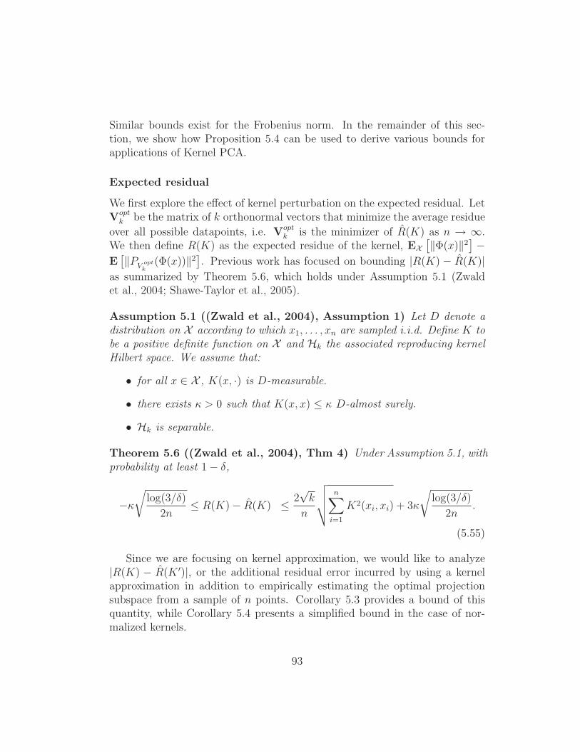
Similar bounds exist for the Frobenius norm. In the remainder of this sec-tion, we show how Proposition 5.4 can be used to derive various bounds forapplications of Kernel PCA.
Expected residual
We first explore the effect of kernel perturbation on the expected residual. LetVopt
k be the matrix of k orthonormal vectors that minimize the average residue
over all possible datapoints, i.e. Voptk is the minimizer of R(K) as n → ∞.
We then define R(K) as the expected residue of the kernel, EX[‖Φ(x)‖2
]−
E[‖PV opt
k(Φ(x))‖2
]. Previous work has focused on bounding |R(K) − R(K)|
as summarized by Theorem 5.6, which holds under Assumption 5.1 (Zwaldet al., 2004; Shawe-Taylor et al., 2005).
Assumption 5.1 ((Zwald et al., 2004), Assumption 1) Let D denote adistribution on X according to which x1, . . . , xn are sampled i.i.d. Define K tobe a positive definite function on X and Hk the associated reproducing kernelHilbert space. We assume that:
• for all x ∈ X , K(x, ·) is D-measurable.
• there exists κ > 0 such that K(x, x) ≤ κ D-almost surely.
• Hk is separable.
Theorem 5.6 ((Zwald et al., 2004), Thm 4) Under Assumption 5.1, withprobability at least 1− δ,
−κ√
log(3/δ)
2n≤ R(K)− R(K) ≤ 2
√k
n
√√√√n∑
i=1
K2(xi, xi) + 3κ
√log(3/δ)
2n.
(5.55)
Since we are focusing on kernel approximation, we would like to analyze|R(K) − R(K ′)|, or the additional residual error incurred by using a kernelapproximation in addition to empirically estimating the optimal projectionsubspace from a sample of n points. Corollary 5.3 provides a bound of thisquantity, while Corollary 5.4 presents a simplified bound in the case of nor-malized kernels.
93

Corollary 5.3 Under Assumption 5.1 and with probability at least 1− δ, thedifference between the expected residual of K and the empirical residual of K ′
is bounded as follows:
|R(K)−R(K ′)| ≤ 2√k
n
√√√√n∑
i=1
K2(xi, xi)+3κ
√log(3/δ)
2n+
(1−k
n
)‖K′−K‖2.
(5.56)
Proof. Using the triangle inequality we have,
|R(K)− R(K ′)| ≤ |R(K)− R(K)|+ |R(K ′)− R(K)| . (5.57)
We bound the first term on the RHS using Theorem 5.6 and bound the secondterm on the RHS using Proposition 5.4. 2
Corollary 5.4 Assume that K(·, ·) is normalized, i.e., K(x, x) = 1 D-almostsurely, as in the case of Gaussian kernels. Then under Assumption 5.1 andwith probability at least 1 − δ, the difference between the expected residual ofK and the empirical residual of K ′ is bounded as follows:
|R(K) − R(K ′)| ≤ 2
√k
n+ 3κ
√log(3/δ)
2n+
(1 − k
n
)‖K′ − K‖2. (5.58)
Subspace perturbation
In the previous analysis, we focused on residuals, which involved projecting thedatapoints onto subspaces spanned by the singular vectors of the covariancematrix. We now focus on the effect of kernel perturbation on the subspaces
themselves. We define PSk= VkV
⊤k and PSk
= Voptk Vopt
k
⊤as the orthogonal
projectors onto the subspaces spanned by the top k singular vectors of theempirical and process covariance matrices, respectively, associated withK(·, ·).Similarly, we define PS′
kas the orthogonal projector onto the subspace spanned
by the top k singular vectors of the empirical covariance matrix associatedwith K ′(·, ·). We would like to analyze ‖PSk
−PS′
k‖F , or the difference in the
approximate empirical subspace and the optimal process subspace. Drawingupon the work of Zwald and Blanchard (2005), as summarized by Theorems5.7 and 5.8, we derive our desired bound on subspace perturbation in Corollary5.5.
94

Theorem 5.7 ((Zwald & Blanchard, 2005), Thm 3) Let K be a kernelmatrix with simple nonzero singular values σ1 > σ2 > . . ., and define k as aninteger such that σk > 0 and ∆k = 1
2(σk − σk+1). Let K′ be a perturbation of
K such that K′ is still positive semidefinite and ‖K−K′‖F ≤ ∆k/2. Then thefollowing bound holds on the difference between the orthogonal projectors ontothe subspaces spanned by the top k singular vectors of the covariance matricesassociated with K and K′:
‖PSk− PS′
k‖F ≤
‖K′ −K‖F∆k
(5.59)
Theorem 5.8 ((Zwald & Blanchard, 2005), Thm 4) Denote the singu-lar values of the kernel operator associated with K(·, ·) by σ1 > σ2 > . . ., anddefine k as an integer such that σk > 0 and ∆k = 1
2(σk − σk+1). Assume that
supx∈X K(x, x) ≤ κ. Define
Bk =2κ
∆k
(1 +
√log(1/δ
2
). (5.60)
Then, with probability at least 1−δ, provided that n ≥ B2k, the following bound
holds on the difference between the orthogonal projectors onto the subspacesspanned by the top k singular vectors of the empirical and process covariancematrices associated with K(·, ·):
‖PSk− PSk
‖F ≤Bk√n
(5.61)
Corollary 5.5 Following the definitions and assumptions of Theorems 5.7and 5.8, then, with probability at least 1 − δ, the following bound holds onthe difference between the orthogonal projectors onto the subspaces spanned bythe top k singular vectors of the empirical covariance matrix associated withK ′(·, ·) and the process covariance matrix associated with K(·, ·):
‖PSk− PS′
k‖F ≤
Bk√n
+‖K′ −K‖F
∆k
(5.62)
Proof. Using the triangle inequality we have,
‖PSk− PS′
k‖F ≤ ‖PSk
− PSk‖F + ‖PSk
− PS′
k‖F . (5.63)
95

Next, we bound the first term on the RHS using Theorem 5.8 and bound thesecond term on the RHS using Theorem 5.7. 2
In summary, Corollaries 5.3 and 5.4 show the connections between ex-pected residuals and the reconstruction error of the sample kernel matrix dueto kernel perturbation. Similarly, Corollary 5.5 shows the connection betweenthis reconstruction error and subspace perturbation. Together, these resultsgeneralize previous theory on expected residuals and subspace perturbation toalso account for the effect of perturbations of the empirical kernel matrix.
5.3.6 Application to Nystrom method
The previous section provided stability analyses for several common learningalgorithms, studying the effect of using an approximate kernel matrix insteadof the true one. The difference in hypothesis value is expressed simply in termsof the difference between the kernels measured by some norm. Although thesebounds are general bounds that are independent of how the approximationis obtained (so long as K′ remains SPSD), one relevant application of thesebounds involves the Nystrom method. As shown by Williams and Seeger(2000), later by Drineas and Mahoney (2005); Talwalkar et al. (2008); Zhanget al. (2008), low-rank approximations of the kernel matrix via the Nystrommethod can provide an effective technique for tackling large-scale data sets.However, all previous theoretical studies analyzing the performance of theNystrom method have focused on the quality of the low-rank approximations,rather than the performance of the kernel learning algorithms used in con-junction with these approximations. In this section, we show how we canleverage kernel stability analysis to present novel performance guarantees forthe Nystrom method in the context of kernel learning algorithms.
Nystrom Kernel Ridge Regression
The accuracy of low-rank Nystrom approximations was discussed in Section5.1. The following corollary, which is a simplified adaptation of Theorem 5.2,gives an upper bound on the norm-2 error of the Nystrom approximation ofthe form ‖K−K‖2/‖K‖2 ≤ ‖K−Kk‖2/‖K‖2 +O(1/
√l). We denote by Kmax
the maximum diagonal entry of K.
Corollary 5.6 Let K denote the rank-k Nystrom approximation of K basedon l columns sampled uniformly at random with replacement from K, and Kk
96

the best rank-k approximation of K. Then, with probability at least 1− δ, thefollowing inequalities hold for any sample of size l:
‖K− K‖2 ≤ ‖K−Kk‖2 + n√lKmax
(2 + log 1
δ
).
Corollary 5.6 focuses on the quality of low-rank approximations. Combiningthe analysis from Section 5.3.1 with this corollary enables us to bound the rela-tive performance of the kernel learning algorithms when the Nystrom methodis used as a means of scaling kernel learning algorithms. To illustrate thispoint, Theorem 5.9 uses Proposition 5.1 along with Corollary 5.6 to upperbound the relative performance of KRR as a function of the approximationaccuracy of the Nystrom method (a similar technique can be used to boundthe error of the Nystrom approximation when used with the other algorithmsdiscussed in Section 5.3).
Theorem 5.9 Let h′ denote the hypothesis returned by Kernel Ridge Regres-sion when using the approximate rank-k kernel K ∈ R
n×n generated using theNystrom method. Then, with probability at least 1− δ, the following inequalityholds for all x ∈ X,
|h′(x)− h(x)| ≤ κM
λ20n
[‖K−Kk‖2 + n√
lKmax
(2 + log 1
δ
)].
We note that the experimental results of Figure 3.9 are useful in analyz-ing our theoretical analysis. In these experiments, we generated approximatekernel matrices using the Nystrom method, and for approximations of vary-ing quality we measured the perturbation of associated KRR hypotheses (seeSection 3.2.2 for details of the experimental design). The experimental resultssuggest a linear relationship between kernel approximation and hypothesisperturbation, which corroborates the shape of the bound in Proposition 5.1.
5.4 Summary
In this section we presented a variety of analyses of the Nystrom method inthe context of machine learning. We first presented theoretical results com-paring the quality of the Nystrom approximation to the ‘best’ low-rank ap-proximation, under sampling assumptions that are commonly used in practice,namely, uniform sampling without replacement. These bounds hold for both
97

the standard Nystrom method as well as the ensemble Nystrom method. Wethen made a connection between matrix coherence and the performance of theNystrom method. We derived novel coherence-based bounds for the Nystrommethod in the low-rank setting, and presented empirical studies that convinc-ingly demonstrate the ability of matrix coherence to measure the degree towhich information can be extracted from a subset of columns both in thelow-rank and full-rank settings. Finally, we addressed the issue of how kernelapproximation affects the performance of learning algorithms. Our analysis isindependent of how the approximation is obtained and simply expresses thechange in hypothesis value in terms of the difference between the approximatekernel matrix and the true one measured by some norm. We also provided aspecific analysis of the Nystrom low-rank approximation in this context anddiscussed experimental results that support our theoretical analysis.
98

Chapter 6
Conclusion
We addressed the question of how machine learning algorithms, in particularkernel methods, can handle large-scale data. We focused on an attractive so-lution to this problem that involves sampling-based techniques to efficientlygenerate low-rank matrix approximations. In Chapter 2, we answered thequestion of what sampling-based approximation should be used. We discussedtwo common sampling-based methods, providing novel theoretical insights re-garding their suitability for various applications and experimental results moti-vated by this theory. Our results show that one of these methods, the Nystrommethod, is superior in the context of large-scale learning. In Chapter 3, wefocused on the applicability of sampling-based low-rank approximations forpractical applications, showing the effectiveness of approximation techniqueson a variety of problems. In particular, we presented the largest study to-datefor manifold learning using the Nystrom method to extract low-dimensionalstructure from high-dimensional data to effectively cluster face images. Wealso discussed the connection between low-rank matrices and the Woodburyapproximation, reporting good empirical results for Kernel Ridge Regressionand Kernel Logistic Regression using the Nystrom method.
An important open question from these two chapters involves obtaininga better characterization of approximate low-dimensional embeddings, as thistask appears to be closely related to the task of approximating spectral recon-struction, yet the empirical results are quite different. Additionally, a morein-depth study is required to understand the convergence properties of theNystrom Kernel Logistic Regression algorithm and to compare its performancerelative to other optimization techniques, e.g., Gradient Descent, ConjugateGradient, Iterative Scaling, Quasi-Newton, etc.
99

Next, in Chapter 4, we addressed a crucial aspect of these sampling basedalgorithms, namely, the method used to select a subset of columns. We fo-cused our discussion on the Nystrom method given its superior performanceon large-scale tasks in Chapters 2 and 3. We first studied both fixed and adap-tive sampling schemes, and showed that given fixed time constraints, uniformsampling works remarkably well. Next, we introduced a promising ensembletechnique that can be easily parallelized and generates superior approxima-tions, both in theory and in practice.
This area remains ripe for future work. A finer theoretical analysis of ourNystrom adaptive sampling technique is required, perhaps inspired by work in(Deshpande et al., 2006). Additionally, new sampling distributions suggestedin recent work have led to improved theoretical bounds for matrix projectionreconstruction (Drineas et al., 2008; Mahoney & Drineas, 2009). Althoughthese sampling techniques are inefficient to compute as they are derived fromthe singular vectors of K (in the case of a SPSD matrix), perhaps similar sam-pling distributions can be computed more efficiently and be used to generatesuperior low-rank approximations. Alternatively, sampling methods that ac-count for the learning task that will use the resultant low-rank approximationcould also lead to better performance (this idea has been studied by (Bach& Jordan, 2005) for the special case of the Incomplete Cholesky algorithm).Finally, in reference to the ensemble Nystrom algorithm, an interesting avenueof future work involves the use of different types of base learners to generatean ensemble approximation. For instance, base learners could be generatedusing other (or a combination of) sampling schemes discussed in Sections 4.1and 4.2, or even using a variety of low-rank approximation methods, e.g., acombination of Nystrom and Column-sampling approximations.
Finally, in Section 5, we provided a variety of theoretical analyses of theNystrom method. We first presented general guarantees on approximationaccuracy and then introduced coherence-based bounds. We also studied theeffect of matrix approximation on actual kernel-based algorithms. There isroom for improvement in the analysis of the Nystrom method. The first set ofbounds can likely be tightened by performing a direct analysis of the Nystrommethod, rather than using an indirect analysis based on approximation ofmatrix multiplication. The coherence-based bounds can be generalized tomatrices with full-rank, and would be more practically relevant if there existedalgorithms to efficiently estimate the coherence of a matrix to determine theapplicability of the Nystrom method on a case-by-case basis. In terms ofkernel perturbation, future work involves analyzing additional kernel-based
100

algorithms and tightening existing perturbation bounds, especially those forSVMs and SVR.
In summary, we have shown that sampling-based low-rank approximation isan effective tool that extends to large-scale applications the benefits of kernel-based algorithms, namely their empirical effectiveness and solid theoreticalunderpinnings.
101

Bibliography
Achlioptas, D., & Mcsherry, F. (2007). Fast computation of low-rank matrixapproximations. Journal of the ACM, 54.
Allauzen, C., Riley, M., Schalkwyk, J., Skut, W., & Mohri, M. (2007). Open-FST: A general and efficient weighted finite-state transducer library. Con-ference on Implementation and Application of Automata.
Arora, S., Hazan, E., & Kale, S. (2006). A fast random sampling algorithmfor sparsifying matrices. Approx-Random.
Asuncion, A., & Newman, D. (2007). UCI machine learning repository. http://www.ics.uci.edu/∼mlearn/MLRepository.html.
Bach, F. R., & Jordan, M. I. (2002). Kernel Independent Component Analysis.Journal of Machine Learning Research, 3, 1–48.
Bach, F. R., & Jordan, M. I. (2005). Predictive low-rank decomposition forkernel methods. International Conference on Machine Learning.
Baker, C. T. (1977). The numerical treatment of integral equations. Oxford:Clarendon Press.
Balasubramanian, M., & Schwartz, E. L. (2002). The Isomap algorithm andtopological stability. Science, 295.
Belabbas, M., & Wolfe, P. J. (2009). On landmark selection and sampling inhigh-dimensional data analysis. arXiv:0906.4582v1[stat.ML].
Belabbas, M. A., & Wolfe, P. J. (2009). Spectral methods in machine learn-ing and new strategies for very large datasets. Proceedings of the NationalAcademy of Sciences of the United States of America, 106, 369–374.
102

Belkin, M., Matveeva, I., & Niyogi, P. (2004). Regularization and semi-supervised learning on large graphs. Conference on Learning Theory.
Belkin, M., & Niyogi, P. (2001). Laplacian Eigenmaps and spectral techniquesfor embedding and clustering. Neural Information Processing Systems.
Belkin, M., & Niyogi, P. (2006). Convergence of Laplacian Eigenmaps. NeuralInformation Processing Systems.
Boser, B. E., Guyon, I. M., & Vapnik, V. N. (1992). A training algorithm foroptimal margin classifiers. Conference on Learning Theory.
Bousquet, O., & Elisseeff, A. (2001). Algorithmic stability and generalizationperformance. Neural Information Processing Systems.
Boutsidis, C., Mahoney, M. W., & Drineas, P. (2009). An improved approx-imation algorithm for the column subset selection problem. Symposium onDiscrete Algorithms.
Candes, E. J., & Recht, B. (2009). Exact matrix completion via convex opti-mization. Foundations of Computational Mathematics, 9, 717–772.
Candes, E. J., & Romberg, J. (2007). Sparsity and incoherence in compressivesampling. Inverse Problems, 23, 969–986.
Candes, E. J., Romberg, J. K., & Tao, T. (2006). Robust uncertainty princi-ples: exact signal reconstruction from highly incomplete frequency informa-tion. IEEE Transactions on Information Theory, 52, 489–509.
Candes, E. J., & Tao, T. (2009). The power of convex relaxation: Near-optimalmatrix completion. arXiv:0903.1476v1[cs.IT].
Cawley, G., & Talbot, N. (2004). Miscellaneous MATLAB software. http:
//theoval.cmp.uea.ac.uk/matlab/default.html#cholinc.
Chang, E., Zhu, K., Wang, H., Bai, H., Li, J., Qiu, Z., & Cui, H. (2008).Parallelizing Support Vector Machines on distributed computers. NeuralInformation Processing Systems.
Chapelle, O., Scholkopf, B., & Zien, A. (Eds.). (2006). Semi-supervised learn-ing. Cambridge, MA: MIT Press.
103

Cortes, C., Mohri, M., Pechyony, D., & Rastogi, A. (2008). Stability of trans-ductive regression algorithms. International Conference on Machine Learn-ing.
Cortes, C., Mohri, M., & Talwalkar, A. (2010). On the impact of kernelapproximation on learning accuracy. Conference on Artificial Intelligenceand Statistics.
Cox, T. F., Cox, M. A. A., & Cox, T. F. (2000). Multidimensional scaling.Chapman & Hall/CRC. 2nd edition.
de Silva, V., & Tenenbaum, J. (2003). Global versus local methods in nonlineardimensionality reduction. Neural Information Processing Systems.
Deshpande, A., Rademacher, L., Vempala, S., & Wang, G. (2006). Matrixapproximation and projective clustering via volume sampling. Symposiumon Discrete Algorithms.
Donoho, D. L. (2006). Compressed Sensing. IEEE Transactions on Informa-tion Theory, 52, 1289–1306.
Donoho, D. L., & Grimes, C. (2003). Hessian Eigenmaps: locally linear em-bedding techniques for high dimensional data. Proceedings of the NationalAcademy of Sciences of the United States of America, 100, 5591–5596.
Drineas, P. (2008). Personal communication.
Drineas, P., Drinea, E., & Huggins, P. S. (2001). An experimental evaluation ofa Monte-Carlo algorithm for SVD. Panhellenic Conference on Informatics.
Drineas, P., Kannan, R., & Mahoney, M. W. (2006a). Fast Monte Carloalgorithms for matrices II: Computing a low-rank approximation to a matrix.SIAM Journal of Computing, 36.
Drineas, P., Kannan, R., & Mahoney, M. W. (2006b). Fast Monte Carloalgorithms for matrices II: Computing a low-rank approximation to a matrix.SIAM Journal on Computing, 36.
Drineas, P., & Mahoney, M. W. (2005). On the Nystrom method for ap-proximating a Gram matrix for improved kernel-based learning. Journal ofMachine Learning Research, 6, 2153–2175.
104

Drineas, P., Mahoney, M. W., & Muthukrishnan, S. (2008). Relative-errorCUR matrix decompositions. SIAM Journal on Matrix Analysis and Appli-cations, 30, 844–881.
Fergus, R., Weiss, Y., & Torralba, A. (2009). Semi-supervised learning ingigantic image collections. Neural Information Processing Systems.
Fine, S., & Scheinberg, K. (2002). Efficient SVM training using low-rank kernelrepresentations. Journal of Machine Learning Research, 2, 243–264.
Fowlkes, C., Belongie, S., Chung, F., & Malik, J. (2004). Spectral groupingusing the Nystrom method. Transactions on Pattern Analysis and MachineIntelligence, 26, 214–225.
Frieze, A., Kannan, R., & Vempala, S. (1998). Fast Monte-Carlo algorithmsfor finding low-rank approximations. Foundation of Computer Science.
Ghahramani, Z. (1996). The kin datasets. http://www.cs.toronto.edu/∼delve/data/kin/desc.html.
Golub, G., & Loan, C. V. (1983). Matrix computations. Baltimore: JohnsHopkins University Press. 2nd edition.
Goreinov, S. A., Tyrtyshnikov, E. E., & Zamarashkin, N. L. (1997). A theoryof pseudoskeleton approximations. Linear Algebra and Its Applications, 261,1–21.
Gorrell, G. (2006). Generalized Hebbian algorithm for incremental SingularValue Decomposition in natural language processing. European Chapter ofthe Association for Computational Linguistics.
Gu, M., & Eisenstat, S. C. (1996). Efficient algorithms for computing a strongrank-revealing QR factorization. SIAM Journal of Scientific Computing, 17,848–869.
Gustafson, A., Snitkin, E., Parker, S., DeLisi, C., & Kasif, S. (2006). Towardsthe identification of essential genes using targeted genome sequencing andcomparative analysis. BMC:Genomics, 7, 265.
Halko, N., Martinsson, P. G., & Tropp, J. A. (2009). Finding structure withrandomness: Stochastic algorithms for constructing approximate matrix de-compositions. arXiv:0909.4061v1[math.NA].
105
Ham, J., Lee, D. D., Mika, S., & Scholkopf, B. (2004). A kernel view of thedimensionality reduction of manifolds. International Conference on MachineLearning.
Har-peled, S. (2006). Low-rank matrix approximation in linear time,manuscript.
Hastie, T., & Tibshirani, R. (1990). Generalized additive models. Chapmanand Hall.
He, X., Yan, S., Hu, Y., & Niyogi, P. (2005). Face recognition using Laplacian-faces. IEEE Transactions on Pattern Analysis and Machine Intelligence, 27,328–340.
Huang, L., Yan, D., Jordan, M., & Taft, N. (2008). Spectral clustering withperturbed data. Neural Information Processing Systems.
Indyk, P. (2006). Stable distributions, pseudorandom generators, embeddings,and data stream computation. Journal of the ACM, 53, 307–323.
Joachims, T. (1999). Making large-scale Support Vector Machine learningpractical. Neural Information Processing Systems.
Johnson, W. B., & Lindenstrauss, J. (1984). Extensions of Lipschitz mappingsinto a Hilbert space. Contemporary Mathematics, 26, 189–206.
Karsmakers, P., Pelckmans, K., Suykens, J., & hamme, J. V. (2007). Fixed-sizeKernel Logistic Regression for phoneme classification. Interspeech.
Keerthi, S. S., Duan, K. B., Shevade, S. K., & Poo, A. N. (2005). A fast dualalgorithm for Kernel Logistic Regression. Machine Learning, 61, 151–165.
Kumar, S., Mohri, M., & Talwalkar, A. (2009a). Ensemble Nystrom method.Neural Information Processing Systems.
Kumar, S., Mohri, M., & Talwalkar, A. (2009b). On sampling-based approxi-mate spectral decomposition. International Conference on Machine Learn-ing.
Kumar, S., Mohri, M., & Talwalkar, A. (2009c). Sampling techniques for theNystrom method. Conference on Artificial Intelligence and Statistics.
106

Kumar, S., & Rowley, H. (2010). People Hopper. http://googleresearch.
blogspot.com/2010/03/hopping-on-face-manifold-via-people.html.
LeCun, Y., & Cortes, C. (1998). The MNIST database of handwritten digits.http://yann.lecun.com/exdb/mnist/.
Liberty, E. (2009). Accelerated dense random projections. Ph.D. thesis, com-puter science department, Yale University, New Haven, CT.
Littlestone, N., & Warmuth, M. K. (1994). The Weighted Majority algorithm.Information and Computation, 108, 212–261.
Liu, R., Jain, V., & Zhang, H. (2006). Subsampling for efficient spectral meshprocessing. Computer Graphics International Conference.
Liu, T., Moore, A. W., Gray, A. G., & Yang, K. (2004). An investigationof practical approximate nearest neighbor algorithms. Neural InformationProcessing Systems.
Lowe, D. G. (2004). Distinctive image features from scale-invariant keypoints.International Journal of Computer Vision, 60, 91–110.
Mahoney, M. W., & Drineas, P. (2009). CUR matrix decompositions for im-proved data analysis. Proceedings of the National Academy of Sciences, 106,697–702.
Mann, G., McDonald, R., Mohri, M., Silberman, N., & Walker, D. (2009).Efficient large-scale distributed training of conditional maximum entropymodels. Neural Information Processing Systems.
Nystrom, E. (1928). Uber die praktische auflosung von linearen integral-gleichungen mit anwendungen auf randwertaufgaben der potentialtheorie.Commentationes Physico-Mathematicae, 4, 1–52.
Ouimet, M., & Bengio, Y. (2005). Greedy spectral embedding. ArtificialIntelligence and Statistics.
Papadimitriou, C. H., Tamaki, H., Raghavan, P., & Vempala, S. (1998). LatentSemantic Indexing: a probabilistic analysis. Principles of Database Systems.
Platt, J. C. (1999). Fast training of Support Vector Machines using sequentialminimal optimization. Neural Information Processing Systems.
107

Platt, J. C. (2004). Fast embedding of sparse similarity graphs. Neural Infor-mation Processing Systems.
Rokhlin, V., Szlam, A., & Tygert, M. (2009). A randomized algorithm forPrincipal Component Analysis. SIAM Journal on Matrix Analysis and Ap-plications, 31, 1100–1124.
Roweis, S., & Saul, L. (2000). Nonlinear dimensionality reduction by LocallyLinear Embedding. Science, 290.
Rudelson, M. (1999). Random vectors in the isotropic position. Journal ofFunctional Analysis, 164, 60–72.
Rudelson, M., & Vershynin, R. (2007). Sampling from large matrices: Anapproach through geometric functional analysis. Journal of the ACM, 54,21.
Ruston, A. F. (1964). Auerbachs theorem. Mathematical Proceedings of theCambridge Philosophical Society, 56, 476–480.
Saunders, C., Gammerman, A., & Vovk, V. (1998). Ridge Regression learningalgorithm in dual variables. International Conference on Machine Learning.
Scholkopf, B., & Smola, A. (2002). Learning with kernels. MIT Press: Cam-bridge, MA.
Shawe-Taylor, J., & Cristianini, N. (2004). Kernel methods for pattern analy-sis. Cambridge University Press.
Shawe-Taylor, J., Williams, C. K. I., Cristianini, N., & Kandola, J. S. (2005).On the eigenspectrum of the Gram matrix and the generalization error ofKernel-PCA. IEEE Transactions on Information Theory, 51, 2510–2522.
Sim, T., Baker, S., & Bsat, M. (2002). The CMU pose, illumination, and ex-pression database. Conference on Automatic Face and Gesture Recognition.
Smola, A. J. (2000). SVLab. http://alex.smola.org/data/svlab.tgz.
Smola, A. J., & Scholkopf, B. (2000). Sparse Greedy Matrix Approximationfor machine learning. International Conference on Machine Learning.
108

Stewart, G. W. (1999). Four algorithms for the efficient computation of trun-cated pivoted QR approximations to a sparse matrix. Numerische Mathe-matik, 83, 313–323.
Talwalkar, A., Kumar, S., & Rowley, H. (2008). Large-scale manifold learning.Conference on Vision and Pattern Recognition.
Talwalkar, A., & Rostamizadeh, A. (2010). Matrix coherence and the Nystrommethod. arXiv:1004.2008v1[cs.AI].
Tenenbaum, J., de Silva, V., & Langford, J. (2000). A global geometric frame-work for nonlinear dimensionality reduction. Science, 290.
Weinberger, K. Q., & Saul, L. K. (2006). An introduction to nonlinear dimen-sionality reduction by maximum variance unfolding. AAAI Conference onArtificial Intelligence.
Williams, C. K. I., & Seeger, M. (2000). Using the Nystrom method to speedup kernel machines. Neural Information Processing Systems.
Zhang, K., & Kwok, J. T. (2009). Density-weighted Nystrom method forcomputing large kernel eigensystems. Neural Computation, 21, 121–146.
Zhang, K., Tsang, I., & Kwok, J. (2008). Improved Nystrom low-rank approx-imation and error analysis. International Conference on Machine Learning.
Zwald, L., & Blanchard, G. (2005). On the convergence of eigenspaces in Ker-nel Principal Component Analysis. Neural Information Processing Systems.
Zwald, L., Bousquet, O., & Blanchard, G. (2004). Statistical properties ofKernel Principal Component Analysis. Conference on Learning Theory.
109