MULTIVARIABLE CALCULUS NOTES

JAMES MCIVOR

0. Introduction

These are my notes for the course Math 53: Multivariable Calculus, at UC Berkeley, in the summerof 2011. This document is a sketch of what occurs in lecture. In the first third of the course (i.e.,until the first midterm), my presentation will differ somewhat from that of Stewart. The materialis the same, but the order of topics is different. As a result, I ask you in the beginning few weeksto read these notes especially carefully. Later on, as I begin to follow Stewart more closely, thesenotes will be more brief. Please advise me of typos or other mistakes. I will update this documentthroughout the course.

1. Overview

Today I won’t cover anything in great detail, but merely give you a feel for what we will do inthis course. Yet in many ways this lecture is the most important, since one of the hardest thingsabout a course like this is keeping all the ideas and techniques organized in your mind.

So, the broad outline of the course is:

(1) Geometry: Curves and Surfaces in Two and Three Dimensions(2) Calculus of Scalar Functions(3) Calculus of Vector Functions

Here’s a rough idea of what the terms in the above mean:

(1) Curve: Something like a bent line. Such things can be described with one free variable.(2) Surface: Something like a bent plane. Can be described by two free variables.(3) Dimension: the number of variables it takes to describe all the points on an object. Lines

and other curves are one-dimensional, planes and other surfaces are two-dimensional.(4) Scalar: A quantity that can be described by a single number. Physical examples: Temper-

ature, speed.(5) Vector: A quantity which has both magnitude and direction. Physical examples: Velocity,

force.

- Define R2 and R3. Right-hand convention.

So far, you have probably primarily studied functions of one variable, usually written f(x). Heref is the name of the function, and x is the name of the independent variable. We usually have tosay at some point what values x may take. For instance, x may be allowed to be any real number,or just a number between 0 and 1, etc. The possible values for x form what is called the domainof f . The important thing to notice about your previous calculus experience is that the domain wasalways either R or a subset of R, such as [0, 1].

Can we have a function whose domain is R2 instead of R? Certainly, and since the points of R2

consist of two real numbers, the input to such a function will be two real numbers, usually writtenf(x, y). For example, the function f(x, y) = x2 + y2 is a function whose domain is all of R2. Thefunction g(x, y) = 1

xy is a function which takes two inputs x and y, but its domain is not all of R2,

since it is not defined when either x or y is zero. This expression really defines a function whosedomain is all of R2 except the x- and y-axes. In similar fashion we can describe functions whosedomain is R3, for instance h(x, y, z) = xyz2 + y sin(xz).

Thus we have extended the domain of functions from R to R2 and R3. That is, we have givenourselves greater flexibility with the “inputs” of our functions. But what about the outputs? Allthe functions above output just a number, or scalar. We would like functions which output pointsin R2 or R3. We will see that points of R2 or R3 are the same thing as vectors, and so we willcall a function whose outputs are in R2 or R3 a vector function, or vector-valued function, orsometimes a vector field. Often we use capital letters to name vector fields, or sometimes bold-facetype. For example, F (x) = (2x, x3) is a vector field in R2 whose domain is R. The vector fieldH(x, y, z) = (x2y, sin yz, ey) is a vector field in R3 whose domain is also R3.

1

2 JAMES MCIVOR

So our goals will be to first understand what various objects in R2 and R3 look like, and thento study scalar functions on those objects, and finally vector functions. Here’s the most importantthing to remember about this class: if you can keep the different functions straight, the calculuspart will be easy; but if you get the functions muddled, and get mixed up between scalar and vectorfunctions, then all the calculus we do can seem much more complicated than it needs to be.

Once you are comfortable with the idea of functions having many variables, you can ask how todifferentiate them. Once you get used to it, this is very easy. Since you have more than one variable,you have more than one derivative: you can differentiate with respect to each different variable. Saywe have a function f(x, y) of two variables. To differentiate with respect to x we pretend that y isa constant (sometimes I just replace y by 17 or some other obscure number to prevent confusion).Then take a normal derivative with respect to x. This is called the partial derivative of f withrespect to x, and denoted ∂f

∂x .

Example 1.1. If f(x, y) = x2y + x+ xey, then ∂f∂x = 2xy + 1 + ey and ∂f

∂y = x2 + xey.

The concept of integration is slightly more subtle. Let’s say we’re taking a definite integral ofa single-variable real-valued function. Then the information we need is not just a function, butan interval, or region, over which to integrate it. When we allow functions with more than onevariable, we must also allow different regions to integrate over. The reason some students find thelater parts of this course confusing is that there seem to be many types of integrals. But there arereally only three types: line integrals, surface integrals, and volume integrals. The different typesjust depend on the dimension of the region over which we integrate. Line integrals are integrals overa one-dimensional region, such as the x-axis, or some curve. Surface integrals are integrals over atwo-dimensional region, maybe the xy-plane, or a rectangle in the plane, or even a strange curvedsurface, like part of an ellipse, for instance. Both types of integrals involve scalar functions - in fact,it only makes sense to integrate scalar functions. Whenever you see an integral involving a vectorfield (and you will see plenty of these at the end of the course), notice that we always do somethingto reduce the vector field to a scalar before performing the integration. Usually this involves vectoroperations like the dot product.

SUMMARY:- We’ll study functions of several variables.- These are functions whose domains are curves or surfaces in R2 and R3

- If the output is just a number, such a function is called a scalar function.- If the output is a point in R2 or R3 (i.e., a vector), such a function is called a vector function.- Partial derivatives are taken by treating all the other variables as constants.- Integrals only make sense for scalar functions, but there are ways of turning vector functions intoscalar functions, and then integrating these.- There are different types of integrals for scalar functions (line, surface, or volume integals), de-pending on the dimension of the region you want to integrate over.

2. “Cutting Out” Curves and Surfaces by Equations

2.1. The Idea of Cutting Out. There are two fundamentally different ways to describe a curveor a surface. One is by giving equations, and this will be our focus today. Tomorrow we will discussthe other method, using parameters. I like to call the first method “cutting out” curves and surfaces,for reasons that will become clear shortly. Let’s work in R2 for the moment. If I go through andpick out all the points (x, y), with no equations, then what I get is all of R2. But if I instead gothrough and pick out only those points (x, y) which satisfy the equation y − x = 0, then what I getis a line, namely the line y = x. So by picking out only the points satisfying a certain equation,I have focused my attention on a smaller part of R2. While R2 itself is two-dimensional (it’s aplane), the line I picked out by my equation y − x = 0 is a one-dimensional object. We will seethat as a general rule, each equation you impose cuts down the dimension by one. What if I insteaduse the equation y + x = 0? I just get a different line, this one with slope -1 instead of 1. Butstill with this one new equation I have gone from the two-dimensional R2 to a one-dimensional object.

Now suppose I play a new game. Starting with R2 as above, I now go through and pick out onlythose points (x, y) which satisfy both equations y − x = 0 and y + x = 0. What sort of object haveI picked out now? To find out, we simply solve both equations simultaneously. The first equationforces y = x, while the second equation forces y = −x. The only choices of x and y that work are(0, 0), often called simply the origin. Thus by starting with all of R2 and imposing two equations,

MULTIVARIABLE CALCULUS NOTES 3

we are reduced to just one point. A point is regarded as a zero-dimensional object, which is consis-tent with the trend that each equation reduces the dimension by one (please remember that this isnot always so - we’ll see a counterexample shortly).

2.2. Intersections. Now let’s work in R3. Points of R3 are usually denoted (x, y, z), where x, y,and z can be any real numbers. As before, imposing no equations at all gives us all of R3. If weimpose one equation, say x+ y+ z = 0, we get a plane (plot some points and see for yourself). Thisis a two dimensional object, sitting inside the three-dimensional space R3. What if now we imposetwo equations: the original one x+ y+ z = 0, and a new one, say x2 + z2 = 1 (this equation doesn’tinvolve y at all, but that doesn’t matter). The first equation by itself, as we saw, cuts out a planein R3. The second equation, as we will see in a few lectures, describes a cylinder directed along they-axis. Imposing both equations at once turns out to give us an ellipse in R3. It can be visualizedby imagining that we “sliced” the cylinder with the plane, giving a cross-section which is the ellipse.Once again, imposing two equations reduces the original dimension (three) by two, since an ellipseis a one-dimensional object.

So we have seen that you can start with R2 or R3, and “cut out” a nice curve or surface by givingone or more equations: here “cutting” means throwing away all those points that don’t satisfy yourequations. This is like a sculptor, who starts with a huge block of marble (R3), and chisels away theparts of the stone that he/she does NOT want in the final sculpture. An equation is like a chisel,and what it removes is just the points that are NOT satisfied by the equation. Count yourselveslucky you only have to wield an equation and not a chisel!

The other thing we have seen is that imposing more than one equation results in an object whichis the intersection of the objects defined by each equation. Every equation by itself corresponds tosome shape, and when you impose the equations simultaneaously you just select those points thatlie in all of those shapes at once. This makes sense in terms of the chisel analogy - more equationsmeans more chisels, which means more cutting, resulting in a smaller object, and intersecting thingsgives smaller objects.

2.3. Possible Sources of Confusion. One thing you need to be careful of is that sometimes anequation can be ambiguous, and you need to take care whether you are working in R2 or R3. This isrelated to situations such as the above (the surface x2 + z2 = 1), where an equation does not involveone of the variables. Here’s an example demonstrating this ambiguity:

Example 2.1. What shape would you say the equation x2 + y2 = 1 defines?

Most of you would probably say a circle of radius 1. That’s correct if we are working in R2,but false in R3. Why false in R3? For one thing, we said that usually each equation reduces thedimension by one. Well, a circle is a type of curve, hence has dimension one, so we expect to needtwo equations, not one, in order to cut out a circle in R3. When working in R3, there is a variablez which does not appear in the equation x2 + y2 = 1. This is an imporant point: when a variabledoes not appear, all values of that variable are allowed. So what x2 + y2 = 1 cuts out is a circlein the xy-plane, which is extended along the z direction; in other words, a cylinder of radius one inthe z-direction. For another example of this ambiguity, the equation x+ y = 2 cuts out a line in R2,but a plane in R3. As before, this plane is easy to describe: you just draw the original line in thexy-plane, and extend it infinitely in the z-direction.

Another possible source of confusion is that sometimes equations may cut out something thatis really two or more curves, even though we’ll still call it a curve. For instance, what does theequation xy = 0 cut out in R2? The equation has solutions whenever either x or y is zero. Thishappens along the y- and x-axes, respectively. So the “curve” cut out by xy = 0 is really a unionof two lines. This is not really a problem, just slightly confusing terminology: “curve” for what youmight normally call “two curves” or “two lines”. Most of the equations we’ll run into will just cutout one curve, but don’t be alarmed if it looks like two.

2.4. When a new equation does not reduce the dimension of the figure. There remainsone loose end to tie up: we have used heavily the “dimension-drop” phenomenon, whereby eachextra equation reduces the dimension of the object under consideration. I mentioned that this doesnot always hold, and I must now show you why, so you know when to use it and when not. The

4 JAMES MCIVOR

only time when the dimension drop does not work is when the extra equation imposed is redundant.For example, the equation x = 0 cuts out a line in R2, namely the y-axis. But so does the equation5x = 0, since multiplying both sides by 5 doesn’t change the solution set to the equation. So if wefirst impose the equation x = 0, and then impose a second equation 5x = 0, the dimension does notdrop - in fact, nothing at all changes. Imposing one equation is the same thing as imposing both.The second equation was redundant. Here is another example:

Example 2.2. Analyze the figure cut out by x2 + y2 + z2 = 25, y = 3, and x2 + z2 = 16

If we just obey the dimension-drop rule, we expect something zero-dimensional. Let’s see thatthis is not so: first impose x2 + y2 + z2 = 25 and y = 3, then impose x2 + z2 = 16. Geometrically,the first equation describes a sphere of radius 5 in R3, and the equation y = 3 describes a plane.To see what they cut out together, we intersect the sphere and the plane, giving us a circle whichlives in the plane y = 3. If you do a little algebra, you can see that the radius of this circle is 4.Thus the third equation tells us nothing new. We started with R3 (3-dimensional), cut out a sphere,which is a type of surface (2-dimensional), then cut out a plane and intersected it with our sphere,giving a circle (1-dimensional). But when we imposed the third equation, we did not drop downto a 0-dimensional object, which is just a set of points, but stayed where we were, since the thirdequation followed from the first two. Notice, however, that what’s cut out by the third equationisn’t the same thing as that cut out by the first two, since the third by itself cuts out a cylinder,whereas the first two determine just a circle.

2.5. SUMMARY. - Equations cut out geometric objects in R2 and R3.- The set of points satisfying the equation(s) are the points on the geometric object.- Imposing more than one equation corresponds to intersecting the associated geometric objects -more equations (usually) means smaller objects.- Usually each extra equation reduces the dimension of the object, unless the equation is redundant.- Keep track of whether you’re in R2 or R3, so you don’t confuse lines for planes, or circles forcylinders, etc.

3. Describing Curves and Surfaces by Parameters

3.1. Parametrizations. Today we discuss the second of the two main approaches to describingcurves and surfaces: parametrization. Roughly speaking, a parametrization is a point in R2 orR3 which changes as the values of the parameter(s) change. By varying the parameter, we canpick out all the points on the curve or surface in which we are interested. As usual, we shouldspecify at the outset whether we are working in R2 or R3. First let’s consider only curves in R2.Curves are one-dimensional, and require only one parameter (for us, this is basically the definitionof “one-dimensional”). Since we’re in R2, we will write down a point (x(t), y(t)) in R2, where thex- and y- coordinates depend on a parameter t. For example, (t, t2) is a parametrization of a curve.So is (cos t, sin t). We think of t as being a time parameter, so as time changes, the point in R2

varies. It is useful to imagine the coordinates (x(t), y(t)) describing the location of a moving particleat time t. Sometimes a parametrization is just given by expressing x and y as functions of t, forinstance, x(t) = 2t, y(t) = 5t describes a line of slope 5/2 through the origin. This is equivalentto putting the two functions together as an ordered pair and referring to the parametrization (2t, 5t).

3.2. Going From Parameters to Cutting Out. If you’re given a parametrization and want toknow what it looks like, you can just plot some points for various values of t. This is often goodenough to give you an idea of what the curve looks like. Usually you should put a little arrow on thecurve to indicate the direction of increasing t. Having spent an entire lecture on describing curves(and surfaces) by equations, it would also be nice to know how to translate between a parametrizedcurve and an equation. This is easy to do. The parametrization involves a new variable, t, namelyx(t) = ... and y(t) = ..., whereas the equation which cuts out the curve will just be an equationinvolving x and y. So to get from the parametrization to the equation involving x and y only, onejust eliminates t from the two equations. When performing the algebra, it’s handy to just write xfor x(t) and y for y(t).

For instance, to express the parametrization x(t) = 2t and y(t) = 5t of the line from above as anequation, we must remove t from the system x = 2t, y = 5t. The first equation say that t = x/t,

MULTIVARIABLE CALCULUS NOTES 5

and plugging this into the second equation gives y = 5x/2. Here’s another:

Example 3.1. Write the equation which cuts out the ellipse (2 cos t, 3 sin t) in R2.

We have to use the equations x = 2 cos t and y = 3 sin t to get one equation which relates xand y. Usually you’ll try to solve for t and substitute. Here it’s easier to isolate the trig functionsand use the Pythagorean identity: Since x/2 = cos t and y/3 = sin t, the Pythagorean identitycos2 t + sin2 t = 1 yields (x2 )2 + (y3 )2 = 1, which is the equation of an ellipse, as we’ll see in a fewlectures.

3.3. Curves in R3. What about curves in R3? The same idea applies: we express the three coor-dinates x, y, and z of R3 each as functions of t, and we imagine this as describing the location of aparticle in three-dimensional space for all values of time. Here’s a classic example:

Example 3.2. The helix in R3 is parametrized by x(t) = cos t, y(t) = sin t, and z(t) = t. Draw apicture of this curve.

If you want to find equations for a parametrized curve in R3, remember first that it takes twoequations to cut out a curve in R3 (one equation alone would cut out a surface). So we have to takethe three expression for x, y, and z in terms of t and eliminate t to get two equations involving x, y,and z. This can often be surprisingly difficult, and I will only ask you to do it for manageable cases.Here’s an example that illustrates how this can be a little tricky.

Example 3.3. A “slanted” ellipse in R3 is parametrized by (cos t, sin t, cos t). Find its definingequations.

Intuitively, the x, y-coordinates are going around in a circle, while the z-coordinate (the “height”)is oscillating. But even without getting an idea of what it looks like, we can let algebra do the talk-ing: The x, y-coordinates satisfy x2 +y2 = 1, and the y, z-coordinates satisfy y2 +z2 = 1. These twoequations nearly cut out our ellipse: since combining equations corresponds to intersecting surfaces,the curve cut out by these two equations is the intersection of two cylinders - one directed upwards,along the z-axis, and the other directed horizontally along the x-axis (the direction in which a cylin-der extends is along the axis corresponding to the variable which does NOT appear in the equationcutting out the cylinder). This intersection of two cylinders should be fairly easy to visualize ordraw. Then you see that it actually consists of two ellipses! So the most natural two equations forthe ellipse cut out not one but two ellipses, and these are NOT the right defining equations. To getthe right ones, you have to notice that any ellipse must lie in a plane. The plane containing our el-lipse can be identified by the fact that the x- and z-coordinates of our parametrization are the same.Thus our ellipse lies in the plane cut out by x = z. What is the other equation? Well, we can just useone of the cylinders from before. So two equations that cut out this ellipse are x = z and x2+y2 = 1.

The above example also illustrates two important points from the previous lecture: (1) there aremany sets of equations which cut out a given curve or surface, and (2) sometimes what we call a“curve” may really be a union of two objects which are curves, as in the pair of ellipses encounteredabove.

3.4. Parametrizing Surfaces. So much for curves in R2 and R3. What about surfaces? This isonly interesting in R3, since the only surfaces that live in R2 are flat, for instance R2 itself. So let’swork in R3, where we must parametrize the three coordinates x, y, and z. Using only one parameterwill give us a curve, but if we use two parameters, say s and t, we get a two-dimensional object,i.e., a surface. So to give a parametrized surface is to give three expressions: one for x in terms ofs, t, one for y in terms of s, t, and one for z in terms of s, t. As before, it is possible to “translate”a parametrized surface into one given by an equation: you have to eliminate s and t to obtain oneequation relating x, y, and z. Here are a few examples:

Example 3.4. (1) x = s+ t; y = s− t; z = 2t. This surface is a plane. The first two equationscan be subtracted to give x − y = 2t, hence x − y = z is the equation that cuts out thisplane. In general, whenever x, y, and z are linear functions of s and t, you get a plane.

6 JAMES MCIVOR

(2) Let’s do a cylinder, since they’ve been coming up so much. Say we want our cylinder toextend along the y-axis and have radius one. Then we should start with a circle (of radiusone) in the xz-plane, and extend it along the y-direction. The circle we want is parametrizedby (cos t, 0, sin t). This is just a curve, since it depends only on the one parameter t. Butwe now allow the y-coordinate to vary depending on a new parameter s, say y = s (wecould choose y = 2s, or y = s3 or any number of others - more on this later). So theparametrization we want is x = cos t; y = s; z = sin t.

(3) This example will be very useful later on. Let x = sin s cos t; y = sin s sin t; z = cos s. Whatsurface does this parametrize? [Hint: first think of t as constant, and see what happens ass changes. For example, at t = 0, what do you get by varying s? Then try to see how thispicture changes as you let t vary also. For another approach, let algebra do the work foryou. Find one equation which these x, y, z satisfy, using the Pythagorean identity. You mayrecognize the surface from the equation.]

3.5. Other Considerations. It is a common source of confusion that any one curve (or surface)has many parametrizations - infinitely many! If you think about the parametrizations as tracking aparticle moving along the curve, then the different parametrizations describe all the different veloc-ities at which the particle may travel. For example, (t, t2) and (2t3, 4t6) both trace out a parabolain the plane, but at different speeds.

There is a very important point that I haven’t mentioned yet. What values are the parametersallowed to take? I have implicitly been letting the parameters range over all the real numbers inthe above discussion. For instance, to describe the whole plane in example (1) above we really needboth s and t to take on all values. But what about the circle in R2 which we parametrized earlierby (cos t, sin t)? Thinking of this as a particle moving in the plane, if we allow all values of time t,the particle goes around the circle over and over again. Sometimes we will be interested in only onerotation, in which case we have to specify off to the side what values of t we are looking at, in thiscase 0 ≤ t ≤ 2π would suffice. Similarly, in example (3) above, I think you will find that 0 ≤ s ≤ 2πand 0 ≤ t ≤ π are enough to describe the whole surface.

Another way to think of this is as follows: a parametrization is like a function, where differentvalues of the parameters are the inputs, and points in R2 or R3 are the outputs. All the previousparagraph says is that sometimes we may want to restrict the domain of these functions. This isactually very useful, and not just a mere technicality, as the following example shows

Example 3.5. Parametrize the semicircle of radius 3 lying in the right half of the plane.

To do this, we want to start with a circle of radius 3 in R2 (sometimes people say“the plane”for R2). This is a curve, so it will involve only one parameter t. In fact, the circle is given byx = 3 cos t; y = 3 sin t. Next we want to restrict the range of t-values so as to only pick out that partof the circle that lies in the right half-plane (in other words, the first and fourth quadrants). Theseare the points whose x-coordinate is non-negative. Since the x-coordinate of our parametrization isx = 3 cos t, we need only values of t for which cos t is non-negative. Letting −π/2 ≤ t ≤ π/2 willwork. So will 3π/2 ≤ t ≤ 5π/2, etc. It is worth pointing out that there’s not really a clean way to

cut this semicircle out with an equation. The best you can do is the equation x =√

9− y2. Theonly reason we would say this cuts out just the semicircle as opposed to the whole circle is becauseit is customary to just take the positive square root. This is just a convention, though, not con-tained in the equation itself. This is a little nitpicky, but the point is, if you want to unambiguouslydescribe the semicircle, you should parametrize it rather than cut it out with an equation, becauseparametrization allows you to restrict the domain of the parameters.

3.6. Piecewise Curves. Another useful thing about restricting the domain is that you can “patchtogether” various curves by taking different parametrizations for different values of time. The resultis sometimtes called a piecewise curve. Students often find these confusing, but it’s really nodifferent than a normal curve - you just have to treat each piece separately and put them alltogether at the end. This is best shown via example:

Example 3.6. What shape does the parametrization

x(t) = t, y(t) = 0 0 ≤ t ≤ 1x(t) = 1, y(t) = t− 1 1 ≤ t ≤ 2x(t) = 3− t, y(t) = 1 2 ≤ t ≤ 3x(t) = 0, y(t) = 4− t 3 ≤ t ≤ 4

MULTIVARIABLE CALCULUS NOTES 7

describe? [Hint: Just draw each part one at a time.] This is another one you can’t cut out withequations.

SUMMARY- The other approach to describing curves and surfaces is to give each of the coordinates in terms ofsome new variables, usually called t (and s, for surfaces).- You can go back and forth between the two descriptions by eliminating the parameter algebraicallyand getting one or more equations involving the original coordinates.- There are many parametrizations of the same curve or surface.- Parametrizations are sometimes more useful than equations, because you can control what valuesof the parameters you want, to describe specific portions of the curve, rather than the whole thing.

4. More on Parameters

Today we study some applications of parametrizations. We’ll focus mostly on curves. First I’llshow you some easy things about a curve that you can just read off from the parametrization. Itis never possible to draw exactly a given curve (even the best computer software still only givesan approximation). Nevertheless there are some easy qualitative aspects which are useful in under-standing what a curve looks like. Next we’ll look at intersections of curves and learn how to tellwhether particles collide. Then we’ll figure out how to find tangent lines to curves (and tangentplanes to surfaces). Finally we’ll learn how to calculate the arc length of a curve.

4.1. Qualitative Characteristics. Firstly, if the values of the parameter t are bounded, you canlocate the start and end points of the curve. If not (e.g., if t is allowed to be any real number), youcan see what happens in the long run by considering the behavior for very large values of t (or verynegative values of t). Sometimes you can also observe that the curve lives only in certain quadrants,by seeing whether the x- and y-coordinates are either always positive or always negative.

Example 4.1. The curve x(t) = 1t cos t, y(t) = 1

t sin t, π ≤ t <∞ starts at the point (− 1π , 0) when

t = π; it has no end point since t can be arbitrarily large. Nevertheless, we can determine the longterm behavior by seeing what happens to each of the coordinates as t goes to infinity. The sine andcosine factors just oscillate back and forth, but the factor of 1

t in each coordinate goes to zero, so ast→∞, the curve approaches the origin. This curve is an inward spiral.

4.2. Colliding Particles. The next thing you might want to do with parametrizations is deter-mine whether two different curves intersect. This is much easier to do when the curves are givenby equations, since, as we have seen, the intersection can be found by solving both equations si-multaneously. So if given two parametrized curves, and asked to find their intersection, I suggestyou either translate into equations and solve the equations, or else just sketch the curves. There isanother interesting question which does involve the parametrization, however: If two particles aremoving in the plane (or in space), how can you determine whether they collide? I illustrate with anexample.

Example 4.2. Two particles, A and B, are moving in the plane. Particle A’s motion is describedby the parametrization (2+2t,−t), and particle B’s motion is described by (2 cos t, sin t). Determinewhen and where, if at all, they collide.

For the particles to collide, two things must happen: (a) the curves along which they move mustintersect; and (b) the particles arrive at the intersection points at the same time. For (a), we convertto the equations which cut out each curve. Particle A moves along a line whose slope is -1/2 andwhose y-intercept is y = 1, which has equation y = 1 − 1

2x. Particle B’s parametrization you may

recognize as that of an ellipse, whose defining equation is x2

4 + y2 = 1. First we determine wherethe line and ellipse meet by solving these equations simultaneously. This gives two points: (0, 1)and (2, 0). These points represent where the curves intersect, but that does not guarantee that theparticles collide - they might each pass through these points at different times. So for each point,we must determine at what times particles A and B arrive there. Particle A passes through (0, 1)at time t = −1 and through (2, 0) at time t = 0. Particle B passes through (0, 1) at t = π/2, 5π/2,So the two particles never meet at (0, 1). But particle B passes through the point (2, 0) at t = 0, 2π,etc. So the particles do collide at (2, 0), at time zero, and this is the only point at which they collide.

8 JAMES MCIVOR

4.3. Tangents. The next thing we’ll do is find tangent lines. If we’re given a parametrized curve(x(t), y(t)), then the slope of the tangent line at the point at time t is given by y′(t)/x′(t) (assum-ing x′(t) 6= 0). This is consistent with the childhood catchphrase “slope is rise over run”, sincethe derivatives of the y- and x-coordinates are just the instantaneous changes in the vertical andhorizontal directions, respectively. If you prefer to remember the formula in Leibniz’ notation:

dy

dx=

dydtdxdt

,

which is easy to remember if you imagine that we are just “cancelling out” the dt. Although theformula is only valid when dx

dt is nonzero; when dxdt is zero (and dy

dt isn’t), we have a vertical tangent.Here’s an example:

Example 4.3. The circle of radius one at the origin is parametrized by (cos t, sin t). At t = π/4 theslope of the tangent line is

dy

dx=

dydt (π/4)dxdt (π/4)

=cosπ/4

− sinπ/4= −1,

which is clear from drawing a picture. Notice that dxdt is zero when t = 0, π, etc: these are the points

with vertical tangent lines.We saw yesterday that there are many parametrizations of the same curve - these correspond toparticles moving around the curve at different speeds. Intuitively, the slope of the tangent linesshould not depend on the speed. Let’s reparametrize the circle and see.

Another perfectly good parametrization of the circle is (cos(t2), sin(t2)). This one goes round alittle slower than the original parametrization until t = 1, and a little faster than the original afterthat. At t = π/4, the previous particle was at the point (

√2/2,√

2/2). The new particle reachesthat point at t =

√π/2. At that time, we compute

dy

dx=

dydt (√π/2)2

dxdt (√π/2)2

=cos((

√π/2)2)(2

√π/2)

− sin((√π/2)2)(2

√π/2)

= −1

For surfaces, there is also a notion of tangent plane. Since a surface has “two degrees offreedom”, i.e., requires two parameters to describe, the tangent plane involves finding slopes “intwo directions”. This will make sense once we study partial derivatives. It is also much easier todescribe planes using the terminology of vectors. So our discussion of tangent planes to surfaces willbe postponed for the moment, but be aware that they exist.

4.4. Arc Length. The final thing we’ll learn to do with a parametrization is compute the lengthof a curve. Needless to say, this is a fundamental notion in geometry. Moreover, we’ll see later howto generalize this calculation to define line integrals, which are one of the fundamental tools of thiscourse. In fact, if you understand the definition of the arc length integral, you can probably guesshow to define a line integral.

Say we have a curve C in R2 which is parametrized by (x(t), y(t)), and we want to compute thelength of that portion of the curve between t = a and t = b. Intuitively, we just add up the lengthsof infinitesimal shreds of the curve. The “length of an infinitesimal shred of the curve”, is denotedds, and is related to the parametrization by the formula

ds =

√(dx

dt

)2

+

(dy

dt

)2

dt,

which may be familiar from computations of surface area of surfaces of revolution in a single-variablecalculus course. The arc length of the curve C is

L(C) =

∫C

ds

which is just a shorthand - it just says the length is computed by adding the arc length element dsup along the entire curve C. The actual calculation is made by the formula

L(C) =

∫ b

a

√(dx

dt

)2

+

(dy

dt

)2

dt.

We’ll do an example in a moment, but let’s have a brief philosophical aside. Why did I botherwriting the formula L(C) =

∫C

ds at all, if we use the formula immediately above to do all the

calculations? The formula L(C) =∫C

ds is like the skeleton of the actual formula. As long as youremember the definition of ds above, and you know that the subscript C means we have to integrateover all of C, and therefore take t from a to b, you can easily write down the longer, more useful

MULTIVARIABLE CALCULUS NOTES 9

version. On the other hand, the skeleton formula can illumniate similarities to other formulas. Inthis case, as I mentioned above, the expression

∫C

ds is a special case of a line integral. These

integrals are usually of the form∫Cfds, where f is a function of x and y. I think the best way to

memorize equations is to just learn the skeletons and know how to expand them into more usefulversions for computational purposes.

Example 4.4. Find the length of the curve (et + e−t, 5 − 2t) from t = 0 to t = 3. Using the arclength formula gives:∫ 1

−1

√(dx

dt

)2

+

(dy

dt

)2

dt =

∫ 1

−1

√(et − e−t)2 + (−2)

2dt

=

∫ 1

−1

√e2t + 2 + e−2tdt

=

∫ 1

−1(et + e−t)dt = 2(e− 1/e)

5. Other Approaches to Visualizing: Graphs and Level Sets

Today we finish the discussion of describing curves and surfaces with a few extra techniques thatwill be very useful once we start doing calculus.

5.1. Parametrizing Graphs of Functions of One Variable. Not every curve is the graph of afunction, but these graphs are probably the most familiar examples of curves. We know two ways todescribe curves (by cutting them out or by a parametrization), so let’s apply these two techniquesto graphs. A function f(x) is not an equation. BUT, if we set y = f(x), we do get an equation,which involves x and y. And an equation involving x and y cuts out a curve in R2, as we have seenalready. This is the relationship between functions and curves. A lot of people get functions andgraphs and curves all confused, so it’s worth thinking this through once more to make sure you havethe ideas straight. Note that if we instead start with a function of y, say g(y), we can obtain itsgraph also: it is cut out by the equation x = g(y).

So we know how, given a function, to find an equation which cuts out the appropriate curve (itsgraph). But what about parametrizing this curve? This is easy. Here’s how:

(1) The graph of a function f of x, which is cut out by y = f(x), is parametrized by (t, f(t)).(2) The graph of a function g of y, which is cut out by x = g(y), is parametrized by (g(t), t).

Example 5.1. (1) Parametrize the part of the graph of f(x) = lnx which lies in the firstquadrant.

Solution: The curve as a whole is parametrized by (t, ln t), according to the rule above.To pick out the part in the first quadrant, we need y to be non-negative (x is already positivesince the domain of ln is the positive real numbers). But y = lnx is non-negative when x ≥ 1.Since x = t in our parametrization, the answer is (t, ln t), t ≥ 1.

(2) Parametrize the part of the ellipsex2

4+y2

9= 1 which lies in the right half-plane, i.e., where

x ≥ 0.

Solution: This is not the graph of a function of x, since it fails the “vertical line test”.However, it is the graph of a function of y, which we can find by solving for x and taking

the positive square root. We get x = 2

√1− y2

9, where the values of y range between -3 and

3 (by looking at the graph). Thus a parametrization of this half-ellipse is(2

√1− t2

9, t

), −3 ≤ t ≤ 3.

5.2. Functions of Two Variables and Their Graphs. A function f(x, y) of two variablestakes the two inputs x and y and outputs a real number. Examples are f(x, y) = sin(xy) andg(x, y) = x3y + 4x2y2. How should we graph this? We can’t do it in R2. The extra variable forcesus to look at the graph in R3. Just as before, we use the function to get an equation z = f(x, y).This equation involves x, y, and z, and therefore cuts out a surface in R3. This surface is the graphof f . To visualize it, you should think of each point in the xy-plane as having another point lyingover it at a certain height z. We calculate the height z by plugging x and y into f .

10 JAMES MCIVOR

How do we parametrize the graph of f(x, y)? Since it’s a surface, we will need two parameters.Just like in the one-variable case, we just set each of the variables equal to the parameters. Thusthe parametrization of the graph of f(x, y) is

(s, t, f(s, t))

You will usually have to specify what values of s, t you are using. Also note that some people will justuse the variables x and y themselves as the parameters, but I like to consistently use the variabless, t for a parametrized surface.

Example 5.2. The “northern hemisphere”, i.e., the top half of the sphere of radius 1, can be

expressed as the graph of the function f(x, y) =√

1− x2 − y2. Thus it can be parametrized by

(s, t,√

1− s2 − t2). Notice, though, that we have to be very careful with the values of s, t allowed,or else the square root is undefined. The allowed values are those s, t which satisfy s+t2 ≤ 1. Thiscorresponds to a disc of radius one in the xy-plane.

5.3. Level Sets. Surfaces tend to be harder to visualize than curves. The rest of the day we’ll lookat a very useful technique for visualizing surfaces, that of level sets. Roughly speaking, a level setis a “slice” or “cross-section” of a surface.

Say you’re given a surface cut out by some equation. The equation will involve x, y, and z. Nowset z equal to fixed number (usually an easy one like 0,1,2, etc.). Let’s say for example we set z = 2.This gives an equation involving only x and y. Often we will know what this looks like - it willbe some curve. This curve is what the surface looks like at the height z = 2, and is called thelevel set for z = 2 (some people call it a level curve). If you draw a few level sets together in thesame plane, and label each one with the appropriate z-value, you get what is called a contour map.

Example 5.3. (1) A sphere is cut out by x2 + y2 + z2 = 1. Let’s look at some level sets. Thelevel set for z = 1 is a point (x = y = 0). The level set for z = 0 is a circle of radiusone x2 + y2 = 1 (this is just the part of the sphere that lives in the xy-plane). The levelset for z = −1/2 is given by x2 + y2 = 3/4 - it’s another circle, but with slightly smallerradius than the one for z = 0. If you stack all these level sets above one another, ordered bythe associated z-values, you can start to see how the sphere is built out of these horizontalcross-sections.

(2) Paraboloid z = x2 + y2

(3) Ellipsoidx2

4+y2

9+z2

16= 1

(4) The graph of f(x, y) = x2y3. [Hint: try plotting level sets for y instead. That is, fix variousy-values and see what the cross-sections in the xz-directions look like.]

6. Polar Coordinates

6.1. Defintions. Polar coordinates r, θ are a new way of locating points in the plane. They replacethe Cartesian coordintes x, y. The point (r, θ) is the point in the plane which is r units away fromthe origin, in a direction which makes an angle θ with the positive x-axis (the angle is measuredcounterclockwise, as usual). The usual trigonometric formula gives us the following relationshipsbetween Cartesian and polar coordinates:

Cartesian to Polar

(1) r =√x2 + y2; θ = tan−1

y

xPolar to Cartesian

(2) x = r cos θ; y = r sin θ

Example 6.1. Express the points whose Cartesian coordinates are (1, 1) and (−2, 0) in polar coor-dinates.

6.2. The Problem - Ambiguity. The annoying thing about polar coordinates is that many pairsof coordinates represent the same point. This is not true for Cartesian coordinates: every point hasa unique pair of Cartesian coordinates. For polar coordinates there are two things to watch out for:

(1) There are many choices of the angle θ, each differing by 2π(2) You may use as the distance from the origin either a positive number r, or −r, but if you

choose −r you must change the angle by π.

Example 6.2. Find all the ways of writing the point (−√

2,√

2) in polar coordinates.

MULTIVARIABLE CALCULUS NOTES 11

6.3. Functions in Polar Coordinates. Given a function f(x), we can obtain a picture of thefunction by setting y = f(x), and seeing what curve this cuts out in the plane. For polar coordinates,the idea is the same, but the pictures end up looking quite different. Given a function f(θ) of thevariable θ, the polar equation r = f(θ) cuts out a curve in the plane. To graph it, you usually thinkof starting at angle θ, and as the angle increases, you track how close or far from the origin you areby finding r from the equation r = f(θ). Let’s look at some examples:

Example 6.3. (1) r = 2 (this is a function of θ - a constant function)(2) θ = π/3 (this is not a function of θ, but it still cuts out a curve)(3) r = θ(4) r = sin θ (contrast with Cartesian curve)(5) r = 1 + sin θ(6) r = 2 + 3 cos 2θ

6.4. Cartesian Equations for Polar Curves. You can use equations (1) and (2) above to trans-late between the Cartesian and Polar equations which cut out a given curve. Let’s do this for theexamples above.

(1) x2 + y2 = 4

(2) y =√

3x(3) tan(x2 + y2) = y

x (yuck)

(4) r =y

r, so y = r2 = x2 + y2

(5) r = 1 +y

r, so y = r2 − r = x2 + y2 −

√x2 + y2

(6) 2x = r2 − 3r = . . .

6.5. Tangents to Polar Curves. Many students get polar coordinates confused with parametriza-tions. They are different - here’s how, explicitly. A parametrization gives each of the two coordinatesin terms of a third quantity, t (the parameter). Polar coordinates are just a different style of coor-dinate.

The source of the confusion is that there is a useful way to get a parametrization of a curve ifyou’re given a polar equation that cuts it out. Let’s say we want to parametrize the polar curver = f(θ). We might try to turn it into Cartesian coordinates and see whether we recognize a famil-iar parametrization. But polar curves can often be strange and you probably won’t know how toparametrize it by looking at the Cartesian equation that cuts it out.

Instead, to make the polar coordinate θ into a parameter, use the following equations:

(3) x(θ) = f(θ) cos θ; y(θ) = f(θ) sin θ

This is a parametrization of the curve because it gives the two (Cartesian) coordinates x and y asfunctions of the parameter θ (which used to be a coordinate, but now we think of it as a parameterfor x and y). These equations are just the earlier formulae x = r cos θ and y = r sin θ, but we’veplugged in f(θ) instead of r.

This is useful for finding tangents, since we saw two lectures ago how to find the tangents to acurve given a parametrization: use the formula

dy

dx=

dydθdxdθ

.

The product rule lets us computedx

dθ= f ′(θ) cos θ − f(θ) sin θ,

dy

dθ= f ′(θ) sin θ + f(θ) cos θ.

Example 6.4. Find the horizontal tangents of the cardioid of example 4.10(5)

Solution Horizontal tangents when dydθ = 0. Setting dy

dθ = ddθ (1+sin θ) sin θ = cos θ+2 sin θ cos θ =

0 gives cos θ = 0 or sin θ = −1/2. This first equation gives solutions (2n + 1)π/2; the second givesθ = 7π/6, 11π/6, etc. Question: look at the picture of the cardioid. What’s happening at the origin?Our calculation says there should be a horizontal tangent there, but it doesn’t seem right. Whatwent wrong?

12 JAMES MCIVOR

6.6. Symmetry. Here we mention a few shortcuts for sketching polar curves

(1) If changing θ for −θ does nothing, then the curve is symmetric across the x-axis(2) If changing θ for π − θ does nothing, then the curve is symmetric across the y-axis(3) If changing r for −r does nothing, the curve has 180◦ rotational symmetry

6.7. Area and Length. The area of a region bounded by the lines θ = a, θ = b, and the polarcurve r = f(θ) is calculated using the formula

A =

∫ b

a

1

2(f(θ))2dθ

If you’re given f , a, and b, this is as easy as just doing the integral. It gets harder when you haveto determine a and b yourself by looking at the intersection of two polar curves:

Example 6.5. Find the area of the region that lies inside the curve r = 2 + sin θ and outside thecurve r = 3 sin θ.

Solution: It is always helpful to have a picture when doing these. Here’s why: we have to findout where the curves intersect to get the right values of a and b. Solving 2 + sin θ = 3 sin θ gives justθ = π/2. What then should be our a and b? Looking at the picture, we see that the inner curve liesentirely inside the other, meeting only at the point (0, 3). So to find the area, we need to integratethe first function minus the second all the way round the circle, so we may choose a = 0 and b = 2π.

Finally, we can compute arc length using the formula from two lectures ago, since we now knowhow to turn a polar equation for a curve into a (Cartesian) parametrization. Just plug x = f(θ) cos θand y = f(θ) sin θ into the equation for the arc length of a parametrized curve; after simplifying, weobtain the formula

L =

∫ b

a

√r2 +

(dr

dθ

)2

dθ

7. Conic Sections

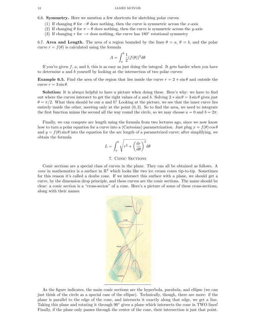
Conic sections are a special class of curves in the plane. They can all be obtained as follows. Acone in mathematics is a surface in R3 which looks like two ice cream cones tip-to-tip. Sometimesfor this reason it’s called a doube cone. If we intersect this surface with a plane, we should get acurve, by the dimension drop principle, and these curves are the conic sections. The name should beclear: a conic section is a “cross-secion” of a cone. Here’s a picture of some of these cross-sections,along with their names

As the figure indicates, the main conic sections are the hyperbola, parabola, and ellipse (we canjust think of the circle as a special case of the ellipse). Technically, though, there are more: if theplane is parallel to the edge of the cone, and intersects it exactly along that edge, we get a line.Taking this plane and rotating it through 90◦ gives a plane which intersects the cone in TWO lines!Finally, if the plane only passes through the center of the cone, their intersection is just that point.

MULTIVARIABLE CALCULUS NOTES 13

Anyway, we’ll focus on the main three in this lecture. There is a huge amount to say aboutconic sections - Apollonius wrote 8 books about them! For this reason, I’ll try to organize in thelecture the main things you need to know. For each type, I will give the general Cartesian equations,describe the curve from a geometric point of view, and then describe it in terms of eccentricity andpolar coordinates.

7.1. Parabolas. These are the sections which occur when the plane is parallel to the edge of thecone. A parabola in the xy-plane can be described as follows. Fix a point F with coordinaes (0, p),called the focus, and a line, say y = −p, called the directrix. Then a parabola is the set of pointswhich are the same distance from the focus as they are from the directix. Given a point (x, y) in the

plane, its distance from the focus is√x2 + (y − p)2 and its distance from the directrix is |y + p|. If

you set these two distances equal to one another and solve for y, you get the equation

y =1

4px2.

[This doesn’t hold if p = 0, but in this case the focus lies on the directrix, and the only point onthe parabola is the origin - not much of a parabola, really.] You can also calculate the equationx = 1

4py2 for the case when the directrix is vertical.

Often you’ll be asked to find the focus and directrix, given an equation of a parabola. If theequation looks like the formula above, you can just read off the value of p and this tells you wherethe focus and directrix are. But this equation only works for a parabola through the origin. Whatif it’s shifted?

Example 7.1. Find the focus and directrix of the parabola cut out by 4x = y2 − 2y − 3.

Solution: Notice that since y is squared, the parabola opens in the horizontal direction. Dosome algebra to write the equation as x+1 = 1

4 (y−1)2. This looks like the equation x = 14y

2, where

p = 1, but it has been shifted to the left by one and up by one. The focus and directrix of x = 14y

2

are (0, 1) and x = −1, respectively, so the focus and directrix of the shifted version are (−1, 2) andx = −2, respectively.

7.2. Ellipses. Normal description: points P such that the sum of the distances from P to F1 andP to F2 are the same. F1 and F2 are the foci.

Let the foci F1 and F2 be at (±c, 0), and call the sum of the distances 2a. Then the ellipse meetsthe x-axis at (±a, 0) (the vertices), and meets the y-axis at (0,±b), where c2 = b2 − a2.

The ellipse is cut out byx2

a2+y2

b2= 1

This description can be thought of as taking a piece of string, and fixing each end to a focus.now take a pencil and use it to pull the string taught. As you move the pencil around, you draw anellipse. The length of the string is the sum of the distances to the foci.

For an ellipse whose major axis is the y-axis, the equation is the same , but the larger number ais in the denominator of the y2 term, and the foci in this case are at (0,±c).

14 JAMES MCIVOR

7.3. Hyperbolae. A hyperbola has equation

x2

a2− y2

b2= 1

There are two foci F1 and F2 at (±c, 0), and points on the hyperbola must be such that theabsolute value of the distance to F1 minus the distance to F2 is constant, equal to 2a. The points(±a, 0) are where the hyperbola meets the x-axis. The hyperbola is a curve which has two separatecomponents, called branches. There are also two asymptotes; these are given by the formulay = ±abx.

7.4. Conic Sections with Polar Coordinates. It may seem that the parabola is the odd one out,since its description involves distances to a point (focus) and a line (directrix), whereas the ellipseand hyperbola are describe in terms of two foci. But there is a description of all three in termsof one focus and a directrix, so the parabola is not so unique as it first seemed. This descriptioninvolves using polar coordinates.

Fix a poinf F and a line L. Then each of the three conic sections above can be described as theset of points P such that the distance from P to F and the distance from P to L always have thesame ratio. This ratio is called the eccentricity e of the conic section

(1) If e < 1 the section is an ellipse(2) If e = 1 it is a parabola(3) If e > 1 it is a hyperbola

If we put the focus F at the origin, these sections have the nice polar equations

(1) r =ed

1 + e cos θfor a vertical directrix x = d

(2) r =ed

1− e cos θfor a vertical directrix x = −d

(3) r =ed

1 + e sin θfor a horizontal directrix x = d

(4) r =ed

1− e sin θfor a horizontal directrix x = −d

Idea of Proof If P = (r, θ), then |PF | = |PL| means r = d− r cos θ. Solve for r to get formula.To decide which conic, can assume it’s not a parabola. In that case, square equation and translate

to Cartesians to identify the familiar equation of the conic. Get a2 =e2d2

(1− e2)2and b2 =

e2d2

1− e2.

For a parabola, we already know what the directrix looks like. For an ellipse it lies on one sideof the curve, and for a hyperbola it lies inbetween the two branches. In both cases the directrix isgiven by the equation d = a2/c.

8. Quadric Surfaces

8.1. Generalities. • Quadric surfaces are 2-D versions of conic sections (their level sets/traces AREconic sections). They are 2-D objects (hence “surface”), but live in R3.

• Quadric surfaces are cut out by quadratic equations in 3 variable (just like conics are cut outby quadratics in two variables)

• Easiest to graph them by looking at their vertical and horizontal traces/level sets (see examples)

• Naming: A something-oid is a shape whose vertical traces are somethings.Example: Paraboloids have vertical traces parabolas, ellipsoids have vertical traces ellipses, etc.

MULTIVARIABLE CALCULUS NOTES 15

• There can be many types of each of these shapes, so sometimes we add another word to describethe horizontal traces (only really used for specifying paraboloids):

Example: elliptic paraboloid has vertical traces parabolas (since it’s a paraboloid in the firstplace), and horizontal traces ellipses.

Example: A hyperbolic paraboloid has vertical traces parabolas and horzontal traces hyper-bolas• Hyperboloids are funny - sometimes they are “broken”, i.e. have two sheets. A hyperboloid

always has vertical traces hyperbolas and horizontal traces ellipses, but sometimes some of thehorizontal traces may be missing. When this happens the hyperboloid has two distinct components,called “sheets”. Thus we distinguish between hyperboloids of one sheet and two sheets.• Q: What about a parabolic ellipsoid, or a parabolic hyperboloid? Why are those not mentioned

in Stewart? A: Because they are elliptic paraboloids and hyperbolic paraboloids oriented alongdifferent axes. The names above describe quadrics which are “oriented along the z-axis”, but theymay be rotated to obtain quadrics oriented along the x- or y-axes instead.

8.2. The Equations That Cut Out Quadrics. The following table summarizes all the equationsfor quadric, as well as which axis they “open along”, under “which way is up”. Horizontal tracesrefer to traces in both the x- and y- directions.

Name Equation Vertical Trace Horizontal Trace Which Way is Up?

Ellipsoidx2

a2+y2

b2+z2

c2= 1 ellipse ellipse

doesn’t matter, they’reall ellipses

EllipticParaboloid

x2

a2+y2

b2=z

cparabola ellipse

the unsquared variableis “up”

HyperbolicParaboloid

x2

a2− y2

b2=z

cparabola hyperbola

the unsquared variableis “up”. The vari-able which is nega-tive has downward par-abolic traces in that di-rection.

Hyperboloid(One Sheet)

x2

a2+y2

b2− z2

c2= 1 hyperbola ellipse

the negative term (theodd one out)

Hyperboloid(Two Sheets)

x2

a2− y2

b2− z2

c2= 1 hyperbola ellipse

the positive term (theodd one out). The topsheet is when z ≥ c,the bottom sheet whenz ≤ −c. Betweenthem, a void.

Cone (degen-erate)

x2

a2+y2

b2=z2

c2hyperbola or two lines ellipse

The lonely one (here,z)

EllipticCylinder(degenerate)

x2

a2+y2

b2= 1 two parallel lines ellipse

The missing variable(here, z)

ParabolicCylinder(degenerate)

y = ax2 one or two parallel lines parabola

The missing vari-able (here, z). Theparabola opens alongthe x- or y-axis asusual.

HyperbolicCylinder(degenerate)

x2

a2− y2

b2= 1 lines hyperbola

The missing variable(here, z). Hyperbolahas axis of symmetryas usual.

Notes:

(1) Even without this table, you can get a quick idea what the traces of quadrics look likeby covering up the variables one at a time. For instance, to determine the trace in the xdirection, just ignore the term involving x and look at the resulting y, z equation. It’s aconic section - which one? That’s the trace in the x-direction.

(2) The equations can be shifted away from the origin by replacing, e.g., x by (x − a), and soon for the other variables.

16 JAMES MCIVOR

(3) The degenerate ones are called degenerate because some of their cross sections are lines,which are degenerate conic sections. Why are they degenerate? Because a conic sectionshould come from a quadratic equation in two variables. The lines occur when all the degreetwo terms are missing - so it’s really a linear equation in two variables, which is technicallystill a quadratic equation, but a degenerate case.

(4) The cylinders all arise whe there are only two variables in the equation. To graph them,just sketch the curve in the xy-plane (or whatever plane involves the two variables present),and extend in the direction of the missing variable.

Example 8.1. (1) (Stewart, 12.6.6) Find traces of and sketch the surface cut out by the equa-tion

4x2 + 9y2 + z = 0.

(2) (Stewart, 12.6.15) Identify and then sketch the surface cut out by

−x2 + 4y2 − z2 = 4

9. The Language of Vectors