Embed Size (px)
Citation preview
Differential Calculus of Multivariable Functions
Introduction to Multivariable Functions
ReadingTrim 12.1−→ Multivariable Functions
12.2−→ Limits and Continuity
Assignmentweb page−→ assignment #3
Functions of Two Independent Variables
If z is uniquely determined when the values of x and y are given, we say that z is a single-valuedfunction of x and y and indicate this fact by the notation
z = f(x, y)
Many engineering applications exist that show this functional dependence, for instance the vibra-tion of a string or the temperature of a plate or a cooling fin
T = f(x, y)
It is sometimes useful to visualize the function graphically. The function z = f(x, y) can bevisualized in two different ways:
1. a contour plot
2. a surface plot
1
Partial Derivatives
ReadingTrim 12.3−→ Partial Derivatives
12.5−→ Higher Order Partial Derivatives
Assignmentweb page−→ assignment #4
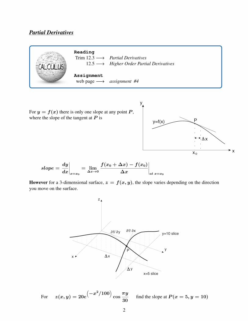
For y = f(x) there is only one slope at any point P ,where the slope of the tangent at P is
slope =dy
dx
∣∣∣∣∣x=x0
= lim∆x→0
f(x0 + ∆x)− f(x0)
∆x
∣∣∣∣∣at x=x0
y
P
xxo
x
y=f(x)
However for a 3-dimensional surface, z = f(x, y), the slope varies depending on the directionyou move on the surface.
For z(x, y) = 20e
(−x2/100
)cos
πy
30find the slope at P (x = 5, y = 10)
2
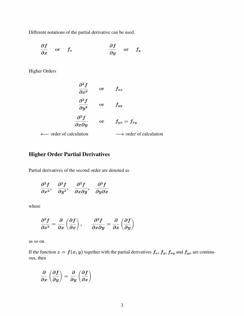
Different notations of the partial derivative can be used.
∂f
∂xor fx
∂f
∂yor fy
Higher Orders
∂2f
∂x2or fxx
∂2f
∂y2or fyy
∂2f
∂x∂yor fyx = fxy
←− order of calculation −→ order of calculation
Higher Order Partial Derivatives
Partial derivatives of the second order are denoted as
∂2f
∂x2,
∂2f
∂y2,
∂2f
∂x∂y,
∂2f
∂y∂x
where
∂2f
∂x2=
∂
∂x
(∂f
∂x
),
∂2f
∂x∂y=
∂
∂x
(∂f
∂y
)
as so on.
If the function z = f(x, y) together with the partial derivatives fx, fy, fxy and fyx are continu-ous, then
∂
∂x
(∂f
∂y
)=
∂
∂y
(∂f
∂x
)
3
Chain Rule for Partial Derivatives
ReadingTrim 12.6−→ Chain Rules for Partial Derivatives
Assignmentweb page−→ assignment #4
Review of Single Variable Functions
• if we understand for 1 variable, it is easy to understand for 2 or 3 variables
• the changes are straight forward
dy
dx=dy
du·du
dx
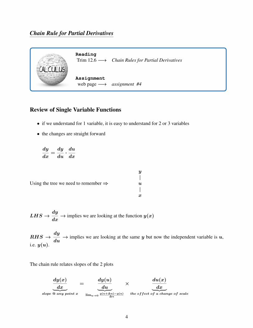
Using the tree we need to remember⇒
y|u|x
LHS →dy
dx→ implies we are looking at the function y(x)
RHS →dy
du→ implies we are looking at the same y but now the independent variable is u,
i.e. y(u).
The chain rule relates slopes of the 2 plots
dy(x)
dx︸ ︷︷ ︸slope @ any point x
=dy(u)
du︸ ︷︷ ︸limu→0
y(u+∆u)−y(u)∆u
×du(x)
dx︸ ︷︷ ︸the effect of a change of scale
4
Chain Rule for Multivariable Functions
1. Given a dependent variable as a function of several independent variables, transform thedependent variable into a new set of independent variables:
z︸︷︷︸dependent
→ independent︷ ︸︸ ︷(u, v) −→ z(x, y)
You will typically be asked to find
∂z
∂x,∂2z
∂x2,∂z
∂y,∂2z
∂y2
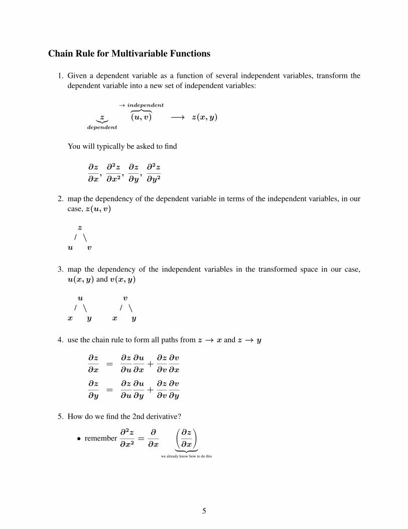
2. map the dependency of the dependent variable in terms of the independent variables, in ourcase, z(u, v)
z/ \
u v
3. map the dependency of the independent variables in the transformed space in our case,u(x, y) and v(x, y)
u v/ \ / \
x y x y
4. use the chain rule to form all paths from z → x and z → y
∂z
∂x=
∂z
∂u
∂u
∂x+∂z
∂v
∂v
∂x
∂z
∂y=
∂z
∂u
∂u
∂y+∂z
∂v
∂v
∂y
5. How do we find the 2nd derivative?
• remember∂2z
∂x2=
∂
∂x
(∂z
∂x
)︸ ︷︷ ︸
we already know how to do this
5
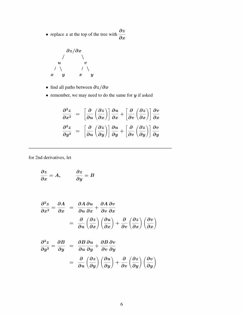
• replace z at the top of the tree with∂z
∂x
∂z/∂x/ \
u v/ \ / \
x y x y
• find all paths between ∂z/∂x
• remember, we may need to do the same for y if asked
∂2z
∂x2=
[∂
∂u
(∂z
∂x
)]∂u
∂x+
[∂
∂v
(∂z
∂x
)]∂v
∂x
∂2z
∂y2=
[∂
∂u
(∂z
∂y
)]∂u
∂y+
[∂
∂v
(∂z
∂y
)]∂v
∂y
for 2nd derivatives, let
∂z
∂x= A,
∂z
∂y= B
∂2z
∂x2=∂A
∂x=
∂A
∂u
∂u
∂x+∂A
∂v
∂v
∂x
=∂
∂u
(∂z
∂x
)(∂u
∂x
)+
∂
∂v
(∂z
∂x
)(∂v
∂x
)
∂2z
∂y2=∂B
∂y=
∂B
∂u
∂u
∂y+∂B
∂v
∂v
∂y
=∂
∂u
(∂z
∂y
)(∂u
∂y
)+
∂
∂v
(∂z
∂y
)(∂v
∂y
)
6
Gradients
ReadingTrim 12.4−→ Gradients
Assignmentweb page−→ assignment #4
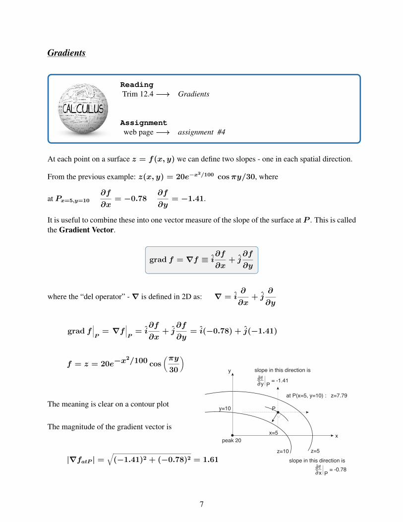
At each point on a surface z = f(x, y) we can define two slopes - one in each spatial direction.
From the previous example: z(x, y) = 20e−x2/100 cosπy/30, where
at Px=5,y=10
∂f
∂x= −0.78
∂f
∂y= −1.41.
It is useful to combine these into one vector measure of the slope of the surface at P . This is calledthe Gradient Vector.
grad f = ∇f ≡ i∂f
∂x+ j
∂f
∂y
where the “del operator” -∇ is defined in 2D as: ∇ = i∂
∂x+ j
∂
∂y
grad f∣∣∣P
= ∇f∣∣∣P
= i∂f
∂x+ j
∂f
∂y= i(−0.78) + j(−1.41)
f = z = 20e−x2/100 cos
(πy30
)
The meaning is clear on a contour plot
The magnitude of the gradient vector is
|∇fatP | =√
(−1.41)2 + (−0.78)2 = 1.61
peak 20
y=10
x=5
z=10 z=5
slope in this direction is
slope in this direction is
f
f
x
y
P
P
= -0.78
= -1.41
y
x
P
at P(x=5, y=10) : z=7.79
7
The gradient vector,∇f is:
• a vector at P that is perpendicular to the contour at P
• points uphill in the direction in which slope increases the most at P
• its magnitude is |∇fatP | = 1.61. If we move 1 unit in the∇f direction, then z increasesby 1.61 units. This is the biggest slope in any direction at P .
The gradient comes up in many applications because things tend to move down the gradient.
Examples:
1. If we release a ball at point P from rest it will roll down the gradient
• the direction will be in the negative∇f direction
• how far it rolls will depend on the magnitude |∇fatP |
2. Heat flow in a cooling fin
• in the cross section of the fin, T = f(x, y)
• the heat flow at some point P is in the∇f direction
• how much heat depends on the magnitude |∇fatP |• Fourier’s law in 2D is ~q = −k∇T
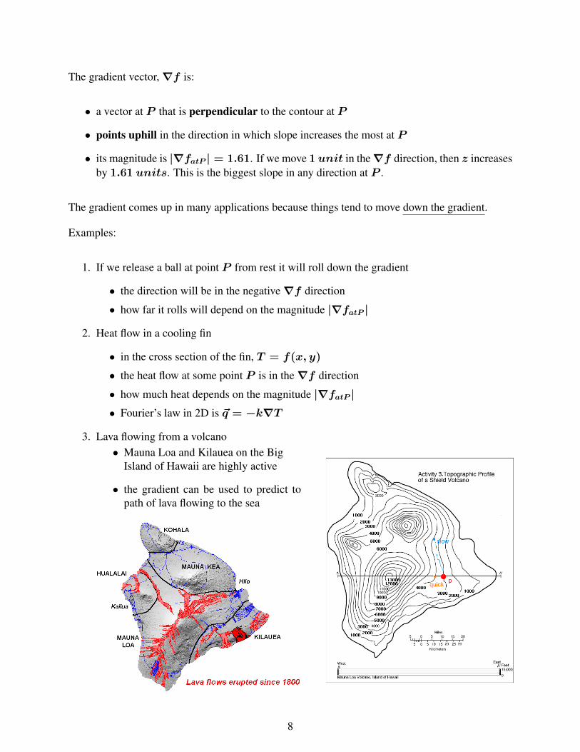
3. Lava flowing from a volcano• Mauna Loa and Kilauea on the Big
Island of Hawaii are highly active
• the gradient can be used to predict topath of lava flowing to the sea
8
Functions of 3 or More Independent Variables
The procedure can be extended to any number of independent variables. In Mechanical Engineer-ing, the biggest number is usually 4. You may have more in abstract applications.
Examples: Solving for the transient temperature response in a room
T = f(x, y, z, t)
Includes 3 spatial variables and 1 time variable. Graphical representation becomes difficult.
Possible graphical representations include:
• multiple contour plots
• level surfaces (surfaces of constant value)
• “slice” - show T vs. z and fixed locations (x0, y0). Need many “slices” for full representa-tion
Gradient in 3-D
For both T = f(x, y, z) and T = f(x, y, z, t) the vector gradient is
∇f = i∂f
∂x+ j
∂f
∂y+ k
∂f
∂z
with the del operator
∇ = i∂
∂x+ j
∂
∂y+ k
∂
∂z
since the gradient vector is a measure in space only. ∇f is a vector in 3-D space. If T =f(x, y, z, t) then∇f will change with time.
Example 2.1
Find the temperature variation inside a spherical lead shield enclosing a small radioactivesphere. The temperature will vary with radius. Suppose for example, that
T = f(x, y, z) =1
√x2 + y2 + z2
where 0.05 ≤ x, y, z ≤ 2
9
Directional Derivatives
ReadingTrim 12.8−→ Directional Derivatives
Assignmentweb page−→ assignment #4
We know how to find a vector that points in the direction of the maximum and minimum changeon slope but how do we account for the rate of change in slope in any other arbitrary direction. Forthis we introduce the directional derivative.
THEOREM: let f(x, y, z) be continuous and possess partial derivatives fx, fy, fz throughoutsome neighborhood of the point P0(x0, y0, z0). Let fx, fy and fz be continuous at P0. Then thedirectional derivative at P0 exists for a unit vector v = (vx, vy, vz) in the direction of v, suchthat
To find the gradient along a line segment s
df
ds=
df
dx︸︷︷︸fx
dx
ds︸︷︷︸vx
+df
dy
dy
ds+df
dz
dz
ds
= fxvx + fyvy + fzvz
where f is expressed in terms of s, where s is a measure of directed distance along a vector andthe unit vector is v = (vx, vy, vz). First set s = 0 at P0 = (x0, y0, z0).
To find f in this transformed space, we can write
x = x0 + vxs
y = y0 + vys
z = z0 + vzs
Note: we start at P0(x0, y0, z0) and attach a vector in the v(vx, vy, vz) direction with a magni-tude of s
10
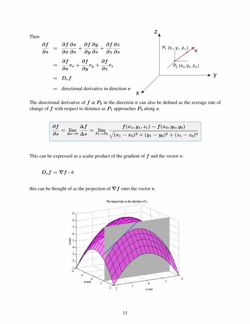
Then
∂f
∂s=
∂f
∂x
∂x
∂s+∂f
∂y
∂y
∂s+∂f
∂z
∂z
∂s
=∂f
∂xvx +
∂f
∂yvy +
∂f
∂zvz
= Dvf
= directional derivative in direction v
P (x ,y ,z )
P (x ,y ,z )
0
1
0
1
0
1
0
1
x
y
z
v
The directional derivative of f at P0 in the direction v can also be defined as the average rate ofchange of f with respect to distance as P1 approaches P0 along s.
∂f
∂s= lim
∆s→0
∆f
∆s= lim
P1→P0
f(x1, y1, z1)− f(x0, y0, y0)√(x1 − x0)2 + (y1 − y0)2 + (z1 − z0)2
This can be expressed as a scalar product of the gradient of f and the vector v.
Dvf = ∇f · v
this can be thought of as the projection of∇f onto the vector v.
11
Tangent Lines and Tangent Planes
ReadingTrim 12.9−→ Tangent Lines and Tangent Planes
Assignmentweb page−→ assignment #4
This is another application of the gradient.
The basic idea is that the∇f is perpendicular to a contour line in 2D and perpendicular to a levelsurface in 3D. Therefore the∇f vector will be perpendicular to a tangent line or plane. We willuse this to find the tangent line or plane at a point.
z = 20e−x2/100 cos(πy
30
)
Find the plane tangent to the surface at point P (x = 5, y = 10).
one way is to use the Taylor series, keeping only the linear terms
z = 7.79− 0.78(x− 5)− 1.41(y − 10)
another way is to use the gradient ideas described above. We can write the equation of the hill as
F (x, y, z) = 20e−x2/100 cos
(πy30
)− z
↪→ move z to the righthand sideif F = 0⇒ on surfaceif F < 0⇒ outsideif F >⇒ inside
In 3D the level surface F = 0 defines the hill surface
∇F = i∂F
∂x+ j
∂F
∂y+ k
∂F
∂z
= i
[20e−x
2/100(−
2x
100
)cos
(πy30
)]
+j[20e−x
2/100 −( π
30
)sin
(πy30
)]+ k(−1)
12
at P (5, 10, 7.79)
∇F |at P = i(−0.78) + j(−1.41) + k(−1)
∇F |at P is perpendicular to the F = 0 surface and also perpendicular to a tangent plane at P .
We have:
• a point on the plane P (5, 10, 7.79)
• a vector normal to the plane ~N = ∇F
Therefore the equation of the tangent plane is
Nx(x− xP ) +Ny(y − yP ) +Nz(z − zP ) = 0
−0.78(x− 5)− 1.41(y − 10)− 1(z − 7.79) = 0
z = 7.79− 0.78(x− 5)− 1.41(y − 10)
This is the same as the Taylor series.
Tangent Plane : A(x− x0) +B(y − y0) + C(z − z0) = 0
Normal Line :x− x0
A=y − y0
B=z − z0
C
where
A = fx(x0, y0), B = fy(x0, y0), C = −1
13
Extrema of Functions
ReadingTrim 12.10−→ Relative Maxima and Minima
12.11−→ Absolute Maxima and Minima
Assignmentweb page−→ assignment #5
Review of Functions of One Variable
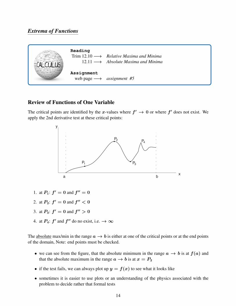
The critical points are identified by the x-values where f ′ → 0 or where f ′ does not exist. Weapply the 2nd derivative test at these critical points:
P
P
P
P
1
2
3
4
y
xa b
1. at P1: f ′ = 0 and f ′′ = 0
2. at P2: f ′ = 0 and f ′′ < 0
3. at P3: f ′ = 0 and f ′′ > 0
4. at P4: f ′ and f ′′ do no exist, i.e.→∞
The absolute max/min in the range a→ b is either at one of the critical points or at the end pointsof the domain, Note: end points must be checked.
• we can see from the figure, that the absolute minimum in the range a → b is at f(a) andthat the absolute maximum in the range a→ b is at x = P2
• if the test fails, we can always plot up y = f(x) to see what it looks like
• sometimes it is easier to use plots or an understanding of the physics associated with theproblem to decide rather that formal tests
14
Functions of Two Variables
We will examine z = f(x, y) where∇f = 0, i.e. the “flat” portion of the curved surface. Thecritical points are where
∂f
∂x= 0
∂f
∂y= 0
In this instance, the 2nd derivative tests involve∂2f
∂x2and
∂2f
∂y2and
∂2f
∂x∂y.
Possible max/min locations include:
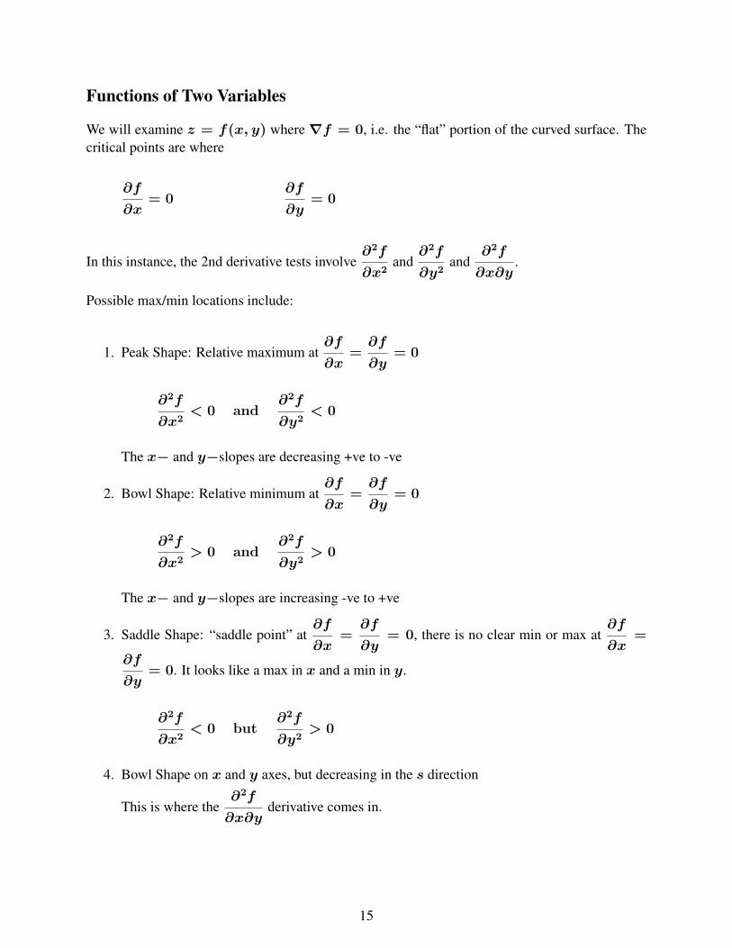
1. Peak Shape: Relative maximum at∂f
∂x=∂f
∂y= 0
∂2f
∂x2< 0 and
∂2f
∂y2< 0
The x− and y−slopes are decreasing +ve to -ve
2. Bowl Shape: Relative minimum at∂f
∂x=∂f
∂y= 0
∂2f
∂x2> 0 and
∂2f
∂y2> 0
The x− and y−slopes are increasing -ve to +ve
3. Saddle Shape: “saddle point” at∂f
∂x=∂f
∂y= 0, there is no clear min or max at
∂f
∂x=
∂f
∂y= 0. It looks like a max in x and a min in y.
∂2f
∂x2< 0 but
∂2f
∂y2> 0
4. Bowl Shape on x and y axes, but decreasing in the s direction
This is where the∂2f
∂x∂yderivative comes in.
15
If the critical point is at P and
∂f
∂x
∣∣∣∣∣P
= 0,∂f
∂y
∣∣∣∣∣P
= 0,
or either or both are undefined at P , then compute
A =∂2f
∂x2
∣∣∣∣∣P
B =∂2f
∂x∂y
∣∣∣∣∣P
C =∂2f
∂y2
∣∣∣∣∣P
D = B2 −AC
if D < 0 and A < 0 ⇒ relative max at P
if D < 0 and A > 0 ⇒ relative min at P
if D > 0 ⇒ saddle point at P
if D = 0 ⇒ test fails - plot to examine
To find the absolute max/min in the interval:
• check f(x, y) values at all critical points and on all the boundary points i.e. edges of theinterval
• the boundary points are more of an issue in 2D than the 1D case
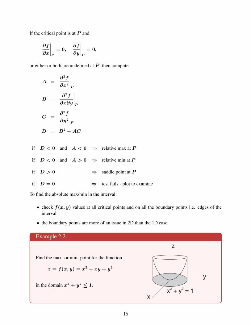
Example 2.2
Find the max. or min. point for the function
z = f(x, y) = x2 + xy + y2
in the domain x2 + y2 ≤ 1.x + y = 1
2 2
x
y
z
16
Constrained Max/Min Problems - Lagrange Multipliers
ReadingTrim 12.12−→ Lagrange Multipliers
Assignmentweb page−→ assignment #6
Problem Statement: An open rectangular box is to have a volume of 0.5m3.Choose the dimensions x, y, z for minimum material to make the box.
Solution Procedure: Let the material needed be equal to the total surface area S.
S = xy + 2yz + 2xz = F (x, y, z) (1)
We want the minimum of f , subject to a constrained equation.
V = xyz = 0.5 (2)
Method 1: apply the constraint by substituting (2) into (1)
From (2)
z = 0.5/(xy)
Therefore,
S = xy + 2y
(0.5
xy
)+ 2x
(0.5
xy
)= xy +
1
x+
1
y
now we want the minimum of f(x, y), where
S = f(x, y)
For a minimum
∂f
∂x= 0
∂f
∂y= 0
17
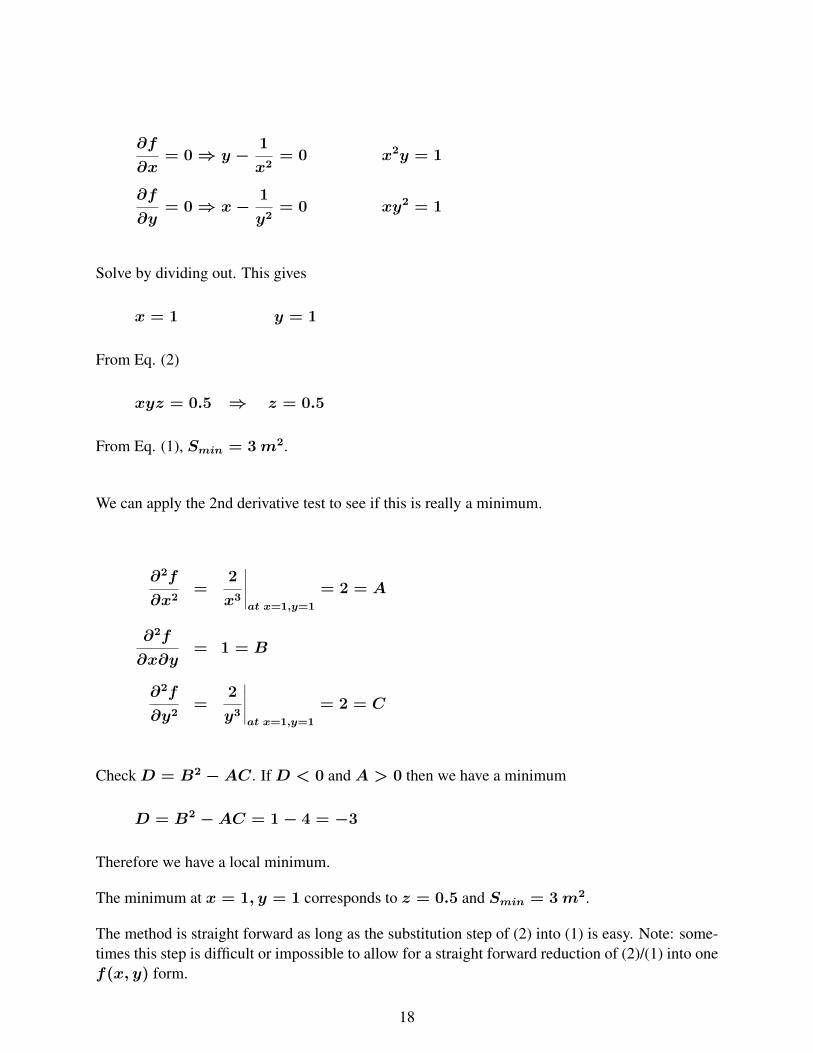
∂f
∂x= 0⇒ y −
1
x2= 0 x2y = 1
∂f
∂y= 0⇒ x−
1
y2= 0 xy2 = 1
Solve by dividing out. This gives
x = 1 y = 1
From Eq. (2)
xyz = 0.5 ⇒ z = 0.5
From Eq. (1), Smin = 3m2.
We can apply the 2nd derivative test to see if this is really a minimum.
∂2f
∂x2=
2
x3
∣∣∣∣∣at x=1,y=1
= 2 = A
∂2f
∂x∂y= 1 = B
∂2f
∂y2=
2
y3
∣∣∣∣∣at x=1,y=1
= 2 = C
CheckD = B2 −AC. IfD < 0 andA > 0 then we have a minimum
D = B2 −AC = 1− 4 = −3
Therefore we have a local minimum.
The minimum at x = 1, y = 1 corresponds to z = 0.5 and Smin = 3m2.
The method is straight forward as long as the substitution step of (2) into (1) is easy. Note: some-times this step is difficult or impossible to allow for a straight forward reduction of (2)/(1) into onef(x, y) form.
18
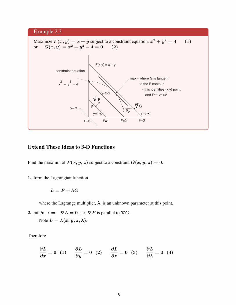
Example 2.3
Maximize F (x, y) = x+ y subject to a constraint equation. x2 + y2 = 4 (1)or G(x, y) = x2 + y2 − 4 = 0 (2)
PP
F=0 F=1 F=2 F=3
F
G1
2
max - where G is tangent
to the F contour
- this identifies (x,y) point
and F valuemax
y=-x
y=1-x
y=2-x
y=3-x
constraint equation
x + y = 42 2
F(x,y) = x + y
Extend These Ideas to 3-D Functions
Find the max/min of F (x, y, z) subject to a constraintG(x, y, z) = 0.
1. form the Lagrangian function
L = F + λG
where the Lagrange multiplier, λ, is an unknown parameter at this point.
2. min/max⇒ ∇L = 0. i.e. ∇F is parallel to∇G.
Note L = L(x, y, z, λ).
Therefore
∂L
∂x= 0 (1)
∂L
∂y= 0 (2)
∂L
∂z= 0 (3)
∂L
∂λ= 0 (4)
19
3. Leads to 4 equations for 4 unknowns - solve for the max/min location - (x, y, z) and the valueof λ, which relates the change in the max/min value of F for small increases or decreases inthe constraint.
It should be noted that the solution can sometimes be difficult, since the 4 equations arenon-linear.
4. once we have x, y, z location, we can evaluate F at the min/max value.
5. the 2nd derivative test of F is possible, but often not necessary.
Example 2.4
Minimize F = xy + 2yz + 2xz (surface area), subject to:
x · y · z = 0.5m3 orG = x · y · z − 0.5 = 0.
20
Method of Least Squares
ReadingTrim 12.13−→ Least Squares
Assignmentweb page−→ assignment #6
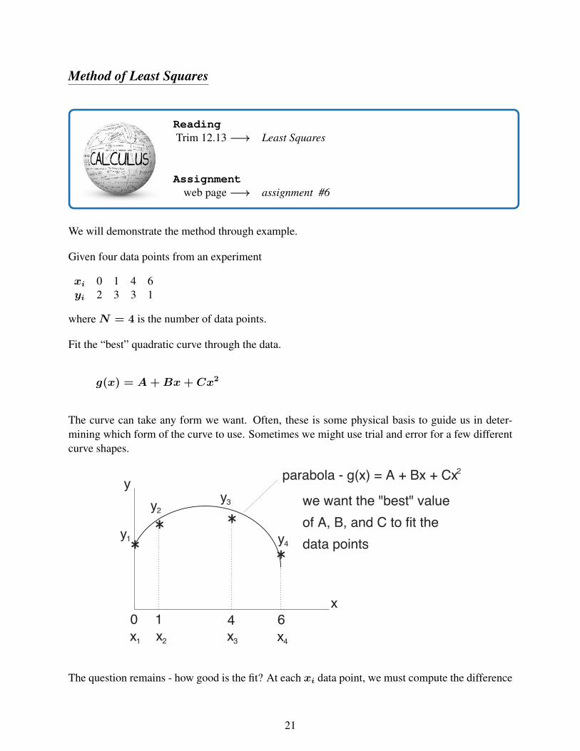
We will demonstrate the method through example.
Given four data points from an experiment
xi 0 1 4 6yi 2 3 3 1
whereN = 4 is the number of data points.
Fit the “best” quadratic curve through the data.
g(x) = A+Bx+ Cx2
The curve can take any form we want. Often, these is some physical basis to guide us in deter-mining which form of the curve to use. Sometimes we might use trial and error for a few differentcurve shapes.
y
y
x x x x
yy
y1
1 2
2
3 4
23
4
x
0 1 4 6
parabola - g(x) = A + Bx + Cx
we want the "best" value
of A, B, and C to fit the
data points
The question remains - how good is the fit? At each xi data point, we must compute the difference
21
(residual). At xi
Ri = g(xi)︸ ︷︷ ︸curve fit value at xi
− yi︸︷︷︸data value at xi
The “best” curve would have minimum Ri summed over all data points. However, some Ri’s are+’ve and some are -’ve. The cancellation effect can be misleading, giving a false indication of agood fit. To avoid this, we need to square Ri, so all are +’ve. Therefore the “best” curve is basedon the minimumR2
i , summed over all points.
The sum of the square of the residuals is given as
S =N∑i=1
[g(xi)− yi]2 =N∑i=1
[A+Bxi + Cx2
i − yi]2
xi and yi are the given data points. The unknowns here areA,B,C. i.e. S = S(A,B,C). Thebest fit will have the minimum value of S. For minimum S
∂S
∂A= 0
∂S
∂B= 0
∂S
∂C= 0
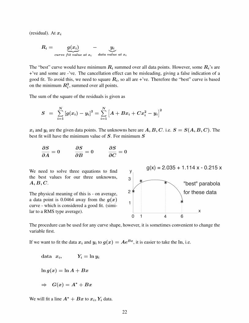
We need to solve three equations to findthe best values for our three unknowns,A,B,C.
The physical meaning of this is - on average,a data point is 0.0464 away from the g(x)curve - which is considered a good fit. (simi-lar to a RMS type average).
y
x
0 1
1
2
3
4 6
g(x) = 2.035 + 1.114 x - 0.215 x
"best" parabola
for these data
The procedure can be used for any curve shape, however, it is sometimes convenient to change thevariable first.
If we want to fit the data xi and yi to g(x) = AeBx, it is easier to take the ln, i.e.
data xi, Yi = ln yi
ln g(x) = lnA+Bx
⇒ G(x) = A∗ +Bx
We will fit a lineA∗ +Bx to xi, Yi data.
22