Mmm

Ma

b

c

a

ARRA

KMFHWS

1

edSwc

UT

(m

h0

Ecological Modelling 279 (2014) 54–67

Contents lists available at ScienceDirect

Ecological Modelling

j ourna l h omepa ge: www.elsev ier .com/ locate /eco lmodel

ultisite-multivariable sensitivity analysis of distributed watershedodels: Enhancing the perceptions from computationally frugalethods

ehdi Ahmadia,∗, James C. Ascough II b, Kendall C. DeJongec, Mazdak Arabia

Department of Civil and Environmental Engineering, Colorado State University, Fort Collins, CO 80523, USAUSDA-ARS, ASRU, 2150 Centre Avenue, Bldg. D, Fort Collins, CO 80526, USAUSDA-ARS, WMRU, 2150 Centre Avenue, Bldg. D, Fort Collins, CO 80526, USA

r t i c l e i n f o

rticle history:eceived 15 October 2013eceived in revised form 9 February 2014ccepted 16 February 2014

eywords:orris sensitivity analysis

ormal likelihood functionydrologyater quality

WAT model

a b s t r a c t

This paper assesses the impact of different likelihood functions in identifying sensitive parameters of thehighly parameterized, spatially distributed Soil and Water Assessment Tool (SWAT) watershed model formultiple variables at multiple sites. The global one-factor-at-a-time (OAT) method of Morris was used forsensitivity analysis of streamflow, combined nitrate (NO3) and nitrite (NO2) fluxes, and total phospho-rous (TP) at five gage stations in a primarily agricultural watershed in the Midwestern United States. TheMorris method was analyzed for 36 combinations of informal likelihood functions, gage stations, andSWAT model output responses, including relative error mass balance (BIAS), Nash–Sutcliffe efficiency(NSE) coefficient, and root mean square error (RMSE) for peak and low fluxes, and one formal likeli-hood function that aggregates information content from multiple sites and multiple variables using 65SWAT parameters. The correlation between sensitivity measures from different likelihood functions wasalso assessed using the Spearman’s rank correlation coefficient. Sensitivity of parameters using differentlikelihood functions was highly variable, although sensitivity of streamflow and TP showed a high cor-relation. A stronger correlation between sensitivity of nutrient fluxes at the upstream stations as well asthe stations closer to the watershed outlets was evident. Comparison of the combined rank of parameters

from informal likelihood functions and the ranks obtained from the formal likelihood function confirmedformal likelihood function ability to effectively identify both sensitive and insensitive parameters withless computational and analysis burden. Uncertainty analysis of the Morris results using bootstrap repli-cations showed that both formal and informal likelihood functions identified sensitive parameters withhigh confidence.

© 2014 Elsevier B.V. All rights reserved.

. Introduction

Watershed-scale hydrologic/water quality (H/WQ) models aressential tools for a wide range of applications, including planning,esign, operation, and management of water resources systems.

tudy of watershed-scale H/WQ fluxes and implementation ofatershed management programs often requires application of

omplex and highly nonlinear models that represent real-world

∗ Corresponding author. Present address: Spatial Science Laboratory, Texas A&Mniversity, 1500 Research Parkway, College Station, TX 77843, USA.el.: +1 979 862 7956.

E-mail addresses: ahmadi@tamu.edu (M. Ahmadi), jim.ascough@ars.usda.govJ.C. Ascough II), kendall.dejonge@ars.usda.gov (K.C. DeJonge),

azdak.arabi@colostate.edu (M. Arabi).

ttp://dx.doi.org/10.1016/j.ecolmodel.2014.02.013304-3800/© 2014 Elsevier B.V. All rights reserved.

physical, biogeochemical, and hydroclimatic characteristics andundergo some degree of conceptualization (Muleta and Nicklow,2005; van Werkhoven et al., 2008). Increased complexity of H/WQmodels is typically associated with an increased number of modelparameters. Establishing scientifically sound and robust H/WQmodel parameters, a process commonly referred to as calibration, isimperative for most watershed-scale H/WQ model applications toensure confidence in model predictions and to avoid implementingfaulty or ineffective watershed management plans (US EPA, 2002;Cotter et al., 2003). However, given the large number of parame-ters in many physically based watershed-scale H/WQ models, it is ofkeen interest to reduce the dimensionality of the calibration prob-

lem by conducting a sensitivity analysis (Campolongo and Saltelli,1997; Feyereisen et al., 2007).

Sensitivity analysis (SA) is “the study of how the uncertaintyin the output of a model can be apportioned to different sources

al Mo

oTtcerIiseHt

oaampdi(2

imeSbcHscSmcHb1MterwGCFCttwii

putmot(pnsms2

M. Ahmadi et al. / Ecologic

f uncertainty in the model input” (Saltelli et al., 2004, p. 45).herefore, SA is closely related to the concept of model uncer-ainty (Saltelli et al., 2000; Helton, 2008). Local SA (LSA) methods,ommonly referred to as classical one-factor-at-a-time (OAT)xperiments, are valuable only if the model can be adequately rep-esented by a first-order polynomial approximation (Cacuci, 2003).n contrast, global sensitivity analysis (GSA) methods explore thenfluence of several input parameters simultaneously and are welluited for complex and highly non-linear watershed-scale mod-ls (Saltelli et al., 1999, 2008; Cacuci and Ionescu-bujor, 2004).owever, GSA methods are also computationally expensive and

herefore less practical (Cacuci, 2003; Campolongo et al., 2007).To address the limitations of both classical OAT and GSA meth-

ds, Morris (1991) proposed a global OAT method that offersn attractive compromise between the accuracy of GSA methodsnd the computational efficiency of classical OAT methods. Theethod of Morris is a screening experiment that covers the entire

arameter space over which input parameters may vary indepen-ently (Cacuci, 2003; Morris, 1991). The Morris method is easy to

mplement and well-suited for sensitivity analysis of large modelsCampolongo and Braddock, 1999; Huang and Liu, 2008; Shen et al.,008; Sun et al., 2012).

The Morris method has proven to be a very useful screen-ng tool to eliminate non-influential parameters from subsequent

odel sensitivity analysis (Campolongo et al., 2007; van Deldent al., 2011), thus the scientific literature is replete with MorrisA applications for large-scale H/WQ modeling. The method haseen used as a screening tool to select important parameters foralibration of various H/WQ models (van Griensven et al., 2002;olvoet et al., 2005; King and Perera, 2013), for uncertainty analy-

is (Shen et al., 2008; Arabi et al., 2007), and for a subsequent moreomputationally intensive sensitivity analysis (Zhan et al., 2013).everal studies have also compared performance of the Morrisethod with other LSA and GSA methods for H/WQ and agroe-

osystem modeling (Francos et al., 2003; Pappenberger et al., 2008;all et al., 2009; DeJonge et al., 2012; Sun et al., 2012). A num-er of studies (e.g., Saltelli et al., 2006; Campolongo and Saltelli,997) showed that ranking of model input parameters using theorris method was very similar, and in some cases identical, to

hose of the more computationally intensive GSA methods. Sev-ral other H/WQ model SA studies have demonstrated satisfactoryanking of sensitive input parameters using the Morris methodith a considerably lower computational cost as compared to theSA methods (see, for instance, Brockmann and Morgenroth, 2007;iric et al., 2012; Confalonieri et al., 2010; DeJonge et al., 2012;rancos et al., 2003; Shen et al., 2008; Zhan et al., 2013). Finally,ampolongo and Saltelli (1997) and DeJonge et al. (2012) showedhat, in addition to similar ranking of sensitive input parameters,he total sensitivity indices of Morris and FAST/Sobol’ methodsere strongly correlated suggesting that the Morris sensitivity

ndices could also be used in a quantitative (rather than only screen-ng) context.

Generally, SA starts with sampling a sufficient number ofarameter sets based on a priori distribution of parameterssing a preferred sampling technique. The model of interest ishen executed for each parameter set to investigate variation of

odel output responses or performance measures. Performancef watershed-scale H/WQ models should be assessed accordingo experimental observations of various environmental processese.g., measured fluxes of water and contaminants), typically sam-led at multiple locations on the watershed stream network. Theumerical measures of disagreement between observed data and

imulated model behavior, often referred to in the literature asodel error, are usually expressed using single-value equations

howing goodness-of-fit or likelihood functions (Fenicia et al.,007; van Griensven et al., 2008).

delling 279 (2014) 54–67 55

An efficient and effective use of observed data is vital forSA of complex, watershed-scale H/WQ models, many of whichare spatially distributed. In the United States, daily or more fre-quent discharge measurements at watershed outlets on manyrivers and streams are available from the United States Geologi-cal Survey (USGS). Conversely, nutrient concentrations are oftenmeasured at less frequent (e.g., weekly or monthly) time-steps atthe smaller sub-watershed level. This is also the case for manyother regions in the world. These types of hydrologic and waterquality observations are characterized by varying measurementerrors/uncertainties, varying sample size and locations, and aretypically non-commensurable. These considerations must be takeninto account when using the data in construction of appropri-ate likelihood function(s) for SA. Selection of a proper likelihoodfunction that reasonably describes distribution of model errors forstatistical inference has important consequences on model perfor-mance analysis results (e.g., Beven and Binley, 1992; Beven andFreer, 2001; Box and Tiao, 1992; Foglia et al, 2009; He et al., 2010;Mantovan and Todini, 2006; Sorooshian and Dracup, 1980; vanGriensven et al., 2008; Wagener et al., 2009). Foglia et al. (2009)and Wagener et al. (2009) suggested the use of multiple likelihoodfunctions (such as low-flow, peak-flow, regression, water balance,and fit-independent likelihood functions) to characterize differentparts of the simulated time series. While thorough, use of severallikelihood functions makes sensitivity analysis of multiple variablesin the watershed-scale H/WQ models complicated and cumber-some.

Beven and Binley (1992) argued that likelihood values of theresponse variables can be combined into a single aggregated value.Several methods are available in the literature for aggregatinglikelihood functions including the pseudo-maximum likelihoodmeasure (van Straten, 1983), multiplication of likelihood func-tions (Beven and Binley, 1992), minimization of the total sum ofsquared residuals (Zak et al., 1997; Madsen, 2003; van Griensvenand Bauwens, 2003), and weighted fuzzy combination (Aronicaet al., 1998). However, the choice of weights and the assump-tion of no correlation between variables make these aggregationmethods statistically less appropriate (DiToro, 1984). Using statis-tically coherent aggregation techniques such as Bayesian statisticsproposed by Ajami et al. (2007), Stedinger et al. (2008), andvan Griensven and Meixner (2007) can potentially dispense withthis restrictive model error assumption for more general applica-tions.

Application of a formal Bayesian-based likelihood function ina parameter estimation practice can provide more acceptableand statistically valid prediction intervals for future observations(Stedinger et al., 2008) and more acceptable posterior distributionof parameters (Vrugt et al., 2009). Ahmadi (2012) showed that useof formal likelihood functions considering the structure of modelerrors are essential in multisite-multivariable performance assess-ment of watershed-scale H/WQ models. While there are a fewstudies that applied formal likelihood functions in calibration ofhydrologic models, to the authors’ knowledge there is no studyon application of formal likelihood functions and aggregation ofH/WQ flux information to quantify sensitivity for H/WQ models atfield-to-watershed scales.

The general objective of this study is to investigate the appli-cation of a statistically correct likelihood function that aggregatesthe information content of multiple variables (processes) mea-sured at several locations within a watershed into a single measureof weighted errors for SA of a physically based, quasi-distributedwatershed model for a Midwestern United States watershed. We

also explore a simplified approach to use the results of the Morrismethod to better understand the complexity of watershed-scaleH/WQ processes including the relationship between fluxes ofnutrients, sediment, and streamflow and the correlation between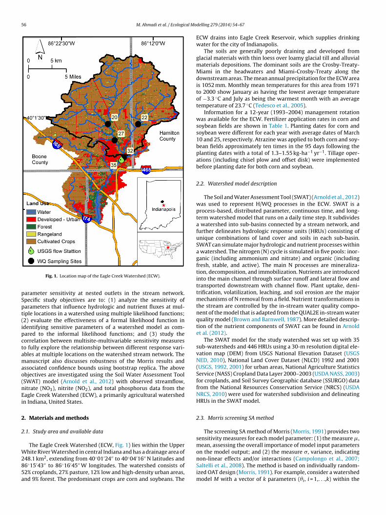

56 M. Ahmadi et al. / Ecological Mo

pSpt(ipctamao(nEi

2

2

W285a

Fig. 1. Location map of the Eagle Creek Watershed (ECW).

arameter sensitivity at nested outlets in the stream network.pecific study objectives are to: (1) analyze the sensitivity ofarameters that influence hydrologic and nutrient fluxes at mul-iple locations in a watershed using multiple likelihood functions;2) evaluate the effectiveness of a formal likelihood function indentifying sensitive parameters of a watershed model as com-ared to the informal likelihood functions; and (3) study theorrelation between multisite-multivariable sensitivity measureso fully explore the relationship between different response vari-bles at multiple locations on the watershed stream network. Theanuscript also discusses robustness of the Morris results and

ssociated confidence bounds using bootstrap replica. The abovebjectives are investigated using the Soil Water Assessment ToolSWAT) model (Arnold et al., 2012) with observed streamflow,itrate (NO3), nitrite (NO2), and total phosphorus data from theagle Creek Watershed (ECW), a primarily agricultural watershedn Indiana, United States.

. Materials and methods

.1. Study area and available data

The Eagle Creek Watershed (ECW, Fig. 1) lies within the Upperhite River Watershed in central Indiana and has a drainage area of

2 ◦ ′ ′′ ◦ ′ ′′

48.1 km , extending from 40 01 24 to 40 04 16 N latitudes and6◦15′43′′ to 86◦16′45′′ W longitudes. The watershed consists of2% croplands, 27% pasture, 12% low and high-density urban areas,nd 9% forest. The predominant crops are corn and soybeans. The

delling 279 (2014) 54–67

ECW drains into Eagle Creek Reservoir, which supplies drinkingwater for the city of Indianapolis.

The soils are generally poorly draining and developed fromglacial materials with thin loess over loamy glacial till and alluvialmaterials depositions. The dominant soils are the Crosby-Treaty-Miami in the headwaters and Miami-Crosby-Treaty along thedownstream areas. The mean annual precipitation for the ECW areais 1052 mm. Monthly mean temperatures for this area from 1971to 2000 show January as having the lowest average temperatureof −3.3 ◦C and July as being the warmest month with an averagetemperature of 23.7 ◦C (Tedesco et al., 2005).

Information for a 12-year (1993–2004) management rotationwas available for the ECW. Fertilizer application rates in corn andsoybean fields are shown in Table 1. Planting dates for corn andsoybean were different for each year with average dates of March10 and 25, respectively. Atrazine was applied to both corn and soy-bean fields approximately ten times in the 95 days following theplanting dates with a total of 1.3–1.55 kg-ha−1 yr−1. Tillage oper-ations (including chisel plow and offset disk) were implementedbefore planting date for both corn and soybean.

2.2. Watershed model description

The Soil and Water Assessment Tool (SWAT) (Arnold et al., 2012)was used to represent H/WQ processes in the ECW. SWAT is aprocess-based, distributed parameter, continuous time, and long-term watershed model that runs on a daily time step. It subdividesa watershed into sub-basins connected by a stream network, andfurther delineates hydrologic response units (HRUs) consisting ofunique combinations of land cover and soils in each sub-basin.SWAT can simulate major hydrologic and nutrient processes withina watershed. The nitrogen (N) cycle is simulated in five pools: inor-ganic (including ammonium and nitrate) and organic (includingfresh, stable, and active). The main N processes are mineraliza-tion, decomposition, and immobilization. Nutrients are introducedinto the main channel through surface runoff and lateral flow andtransported downstream with channel flow. Plant uptake, deni-trification, volatilization, leaching, and soil erosion are the majormechanisms of N removal from a field. Nutrient transformations inthe stream are controlled by the in-stream water quality compo-nent of the model that is adapted from the QUAL2E in-stream waterquality model (Brown and Barnwell, 1987). More detailed descrip-tion of the nutrient components of SWAT can be found in Arnoldet al. (2012).

The SWAT model for the study watershed was set up with 35sub-watersheds and 446 HRUs using a 30-m resolution digital ele-vation map (DEM) from USGS National Elevation Dataset (USGSNED, 2010), National Land Cover Dataset (NLCD) 1992 and 2001(USGS, 1992, 2001) for urban areas, National Agriculture StatisticsService (NASS) Cropland Data Layer 2000–2003 (USDA NASS, 2003)for croplands, and Soil Survey Geographic database (SSURGO) datafrom the National Resources Conservation Service (NRCS) (USDANRCS, 2010) were used for watershed subdivision and delineatingHRUs in the SWAT model.

2.3. Morris screening SA method

The screening SA method of Morris (Morris, 1991) provides twosensitivity measures for each model parameter: (1) the measure �,mean, assessing the overall importance of model input parameterson the model output; and (2) the measure �, variance, indicating

non-linear effects and/or interactions (Campolongo et al., 2007;Saltelli et al., 2008). The method is based on individually random-ized OAT design (Morris, 1991). For example, consider a watershedmodel M with a vector of k parameters (�i, i = 1,. . .,k) within the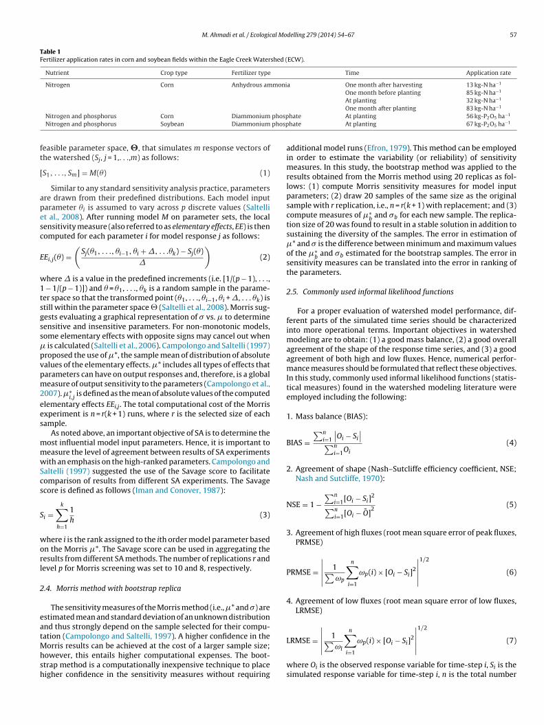

M. Ahmadi et al. / Ecological Modelling 279 (2014) 54–67 57

Table 1Fertilizer application rates in corn and soybean fields within the Eagle Creek Watershed (ECW).

Nutrient Crop type Fertilizer type Time Application rate

Nitrogen Corn Anhydrous ammonia One month after harvesting 13 kg-N ha−1

One month before planting 85 kg-N ha−1

At planting 32 kg-N ha−1

−1

phosp phosp

ft

[

apesc

E

w1tsgss�pvpm2ees

mmwScs

S

worl

2

eatMhsh

Nitrogen and phosphorus Corn DiammoniumNitrogen and phosphorus Soybean Diammonium

easible parameter space, �, that simulates m response vectors ofhe watershed (Sj, j = 1,. . .,m) as follows:

S1, . . ., Sm] = M(�) (1)

Similar to any standard sensitivity analysis practice, parametersre drawn from their predefined distributions. Each model inputarameter �i is assumed to vary across p discrete values (Saltellit al., 2008). After running model M on parameter sets, the localensitivity measure (also referred to as elementary effects, EE) is thenomputed for each parameter i for model response j as follows:

Ei,j(�) =(

Sj(�1, . . ., �i−1, �i + �, . . .�k) − Sj(�)�

)(2)

here � is a value in the predefined increments (i.e. [1/(p − 1), . . ., − 1/(p − 1)]) and � = �1, . . ., �k is a random sample in the parame-er space so that the transformed point (�1, . . ., �i−1, �i + �, . . . �k) istill within the parameter space � (Saltelli et al., 2008). Morris sug-ests evaluating a graphical representation of � vs. � to determineensitive and insensitive parameters. For non-monotonic models,ome elementary effects with opposite signs may cancel out when

is calculated (Saltelli et al., 2006). Campolongo and Saltelli (1997)roposed the use of �*, the sample mean of distribution of absolutealues of the elementary effects. �* includes all types of effects thatarameters can have on output responses and, therefore, is a globaleasure of output sensitivity to the parameters (Campolongo et al.,

007). �∗i,j

is defined as the mean of absolute values of the computedlementary effects EEi,j. The total computational cost of the Morrisxperiment is n = r(k + 1) runs, where r is the selected size of eachample.

As noted above, an important objective of SA is to determine theost influential model input parameters. Hence, it is important toeasure the level of agreement between results of SA experimentsith an emphasis on the high-ranked parameters. Campolongo and

altelli (1997) suggested the use of the Savage score to facilitateomparison of results from different SA experiments. The Savagecore is defined as follows (Iman and Conover, 1987):

i =k∑

h=1

1h

(3)

here i is the rank assigned to the ith order model parameter basedn the Morris �*. The Savage score can be used in aggregating theesults from different SA methods. The number of replications r andevel p for Morris screening was set to 10 and 8, respectively.

.4. Morris method with bootstrap replica

The sensitivity measures of the Morris method (i.e., �* and �) arestimated mean and standard deviation of an unknown distributionnd thus strongly depend on the sample selected for their compu-ation (Campolongo and Saltelli, 1997). A higher confidence in the

orris results can be achieved at the cost of a larger sample size;owever, this entails higher computational expenses. The boot-trap method is a computationally inexpensive technique to placeigher confidence in the sensitivity measures without requiring

One month after planting 83 kg-N hahate At planting 56 kg-P2O5 ha−1

hate At planting 67 kg-P2O5 ha−1

additional model runs (Efron, 1979). This method can be employedin order to estimate the variability (or reliability) of sensitivitymeasures. In this study, the bootstrap method was applied to theresults obtained from the Morris method using 20 replicas as fol-lows: (1) compute Morris sensitivity measures for model inputparameters; (2) draw 20 samples of the same size as the originalsample with r replication, i.e., n = r(k + 1) with replacement; and (3)compute measures of �∗

band �b for each new sample. The replica-

tion size of 20 was found to result in a stable solution in addition tosustaining the diversity of the samples. The error in estimation of�* and � is the difference between minimum and maximum valuesof the �∗

band �b estimated for the bootstrap samples. The error in

sensitivity measures can be translated into the error in ranking ofthe parameters.

2.5. Commonly used informal likelihood functions

For a proper evaluation of watershed model performance, dif-ferent parts of the simulated time series should be characterizedinto more operational terms. Important objectives in watershedmodeling are to obtain: (1) a good mass balance, (2) a good overallagreement of the shape of the response time series, and (3) a goodagreement of both high and low fluxes. Hence, numerical perfor-mance measures should be formulated that reflect these objectives.In this study, commonly used informal likelihood functions (statis-tical measures) found in the watershed modeling literature wereemployed including the following:

1. Mass balance (BIAS):

BIAS =∑n

i=1

∣∣Oi − Si

∣∣∑ni=1Oi

(4)

2. Agreement of shape (Nash–Sutcliffe efficiency coefficient, NSE;Nash and Sutcliffe, 1970):

NSE = 1 −∑n

i=1[Oi − Si]2∑n

i=1[Oi − O]2

(5)

3. Agreement of high fluxes (root mean square error of peak fluxes,PRMSE)

PRMSE =∣∣∣∣∣ 1∑

ωp

n∑i=1

ωp(i) × [Oi − Si]2

∣∣∣∣∣1/2

(6)

4. Agreement of low fluxes (root mean square error of low fluxes,LRMSE)

∣∣∣ 1n∑

2

∣∣∣1/2

LRMSE = ∣∣∑ωli=1

ωp(i) × [Oi − Si] ∣∣ (7)

where Oi is the observed response variable for time-step i, Si is thesimulated response variable for time-step i, n is the total number

5 al Modelling 279 (2014) 54–67

oaflvatptlm

atitniatovfalz

2

d(vm�f

L

acap

,j]2 −

wooomanteaift

�

Fig. 2. Morris sensitivity (�*) of SWAT output responses (Table 3) to input param-eters (Table 2). The x-axis represents combination of informal likelihood functions,

8 M. Ahmadi et al. / Ecologic

f observations, O denotes the mean of observed responses, and ωp

nd ωl are weighting vectors to distinguish between peak and lowuxes. Peak flux events are defined as periods where the observedalue is above a given threshold level. Similarly, low flux eventsre defined as periods where the observed value is below a givenhreshold level. The weights indicate the importance to be given toarticular portions of the response vector, reflecting the errors inhe data and the model (Madsen, 2000). In this study, the thresholdevel of the high and low flows was defined as to be equal to 50% of

ean observed responses (i.e., threshold = 0.5 × O).BIAS, or its percentage expression PBIAS, is a measure of the

verage tendency of simulated values to be greater or smallerhan corresponding observed values and has the ability to clearlyndicate poor model performance (Gupta et al., 1999). BIAS is a par-icularly useful measure for evaluation of model performance forutrients, pesticides, and other contaminants that are addressed

n watershed management programs such as TMDLs based on theverage annual response (Moriasi et al., 2007). The NSE determineshe relative magnitude of the residual variance compared to thebserved data variance. It indicates how well the plot of observedersus simulated values fits the 1:1 line. The coefficient can rangerom –∞ to a perfect match of +1 (ASCE, 1993). PRMSE and LRMSEre measures of absolute deviation between observed and simu-ated values and vary between zero and ∞ with a perfect match ofero.

.6. Formal likelihood function

The formulation of the formal likelihood function depends onistribution of the residuals. For example, assuming that residualse = differences between observed variable O and simulated outputariable S) are normally and independently distributed (NID) withean equal to zero and unknown but constant standard deviation

e, the likelihood function L for each model response can take theollowing form (van Griensven and Meixner, 2007):

(�/O) =n∏

i=1

1√2��(2/e)

exp

[− (Si(�) − Oi)

2

2�(2/e)

](8)

By taking the logarithm of the likelihood function and applying first-order autoregressive (AR-1) transformation to account fororrelated errors (Sorooshian and Dracup, 1980) for multiple vari-bles at multiple observation sites (j = 1 . . . m), a statistically valid,roper likelihood function can be given as (Ahmadi, 2012):

(�|y) =m∑

j=1

{−nj

2ln(2�) − 1

2ln

�2n,jϑ,j

1 − �2j

− 12

(1 − �2j )�−2

ϑ,j[S1,j(�) − O1

here m is the total number of variables, nj is the number ofbserved data for the ith variable, �−2

ϑ,jis the standard deviation

f residuals for the jth variable, and � is the lag − 1 serial coefficientf residuals for the jth variable. The terms �−2

ϑ,jand � can be esti-

ated using the Bayesian approach (Vrugt et al., 2009) or can bessigned based on prior knowledge. In the case that residuals doot have a stable variance, one can use a suitable transformation ofhe residuals (Box et al., 2008; Kuczera and Parent, 1998; Stedingert al., 2008). The transformation proposed by Box and Cox (1964)nd alternate power transformations have been commonly usedn hydrologic modeling. The extended form of the Box–Cox trans-ormation of the simulated and observed hydrologic variables (y)akes the following form as given by Yeo and Johnson (2000):

(y) =

⎧⎨⎩

(y + 2) 1 − 1 1

; if 1 /= 0

log(y + 2); if 1 = 0

(10)

12

�−2ϑ,j

nj∑i=2

{(Oi,j − �jOi−1,j) − [Si,j(�) − �jSi−1,j(�)]}2

}(9)

stations, and output response variable numbers (LSOs) for streamflow (1–4), NOx(5–20), and TP (21–36) as given in Table 3.

where 1 and 2 are transformation parameters. 2 should be cho-sen such that y + 2 > 0 (or 2 > − y) and 1 can be estimated usinga maximum likelihood function. The likelihood function is con-structed based on the assumption that the transformed data �(y) arenormally distributed and the function is maximized with respectto the unknown value ( 1).

2.7. SWAT input parameters and output response variables

Overall, 65 SWAT parameters were selected that are relevantin regard to their ability to affect hydrologic and nutrient fluxes(Table 2). These include surface and subsurface flow, nutrient parti-tioning, and sediment transport parameters that are typically usedin model calibration of the SWAT models (Arnold et al., 2012).Haan et al (1998) and Monod et al. (2006) noted that the rangeof input values usually has more influence on the sensitivity analy-sis results than the distribution shapes. Thus, uniform distributionsbetween the lower and upper bounds of the parameters (Table 2)

were assumed in this study. Given the replications (r = 10), a samplesize of N = 660 was used for the Morris screening method.

Daily streamflow data were available at the watershed outlet(outlet 35 in Fig. 1, USGS gauge no. 03353200) from a USGS gagingstation. Instantaneous samples of nitrate (NO3), nitrite (NO2), andtotal phosphorus (TP) were available at multiple sites on bi-weeklyand monthly basis from Indiana Department of EnvironmentalManagement (IDEM). The sum of NO2 and NO3, referred to as NOxhereafter, and TP data from four sites (outlets 20, 22, 27, and 32 asshown in Fig. 1) were used in this study. Monthly NOx and TP loadswere estimated from concentration data using the LOADEST pro-

gram (Runkel et al., 2004). Statistics were computed for the fourinformal likelihood functions (BIAS, NSE, PRMSE, and LRMSE) foreach response variable at each station. A list of the likelihood func-tions and the corresponding 36 reference numbers (used hereafter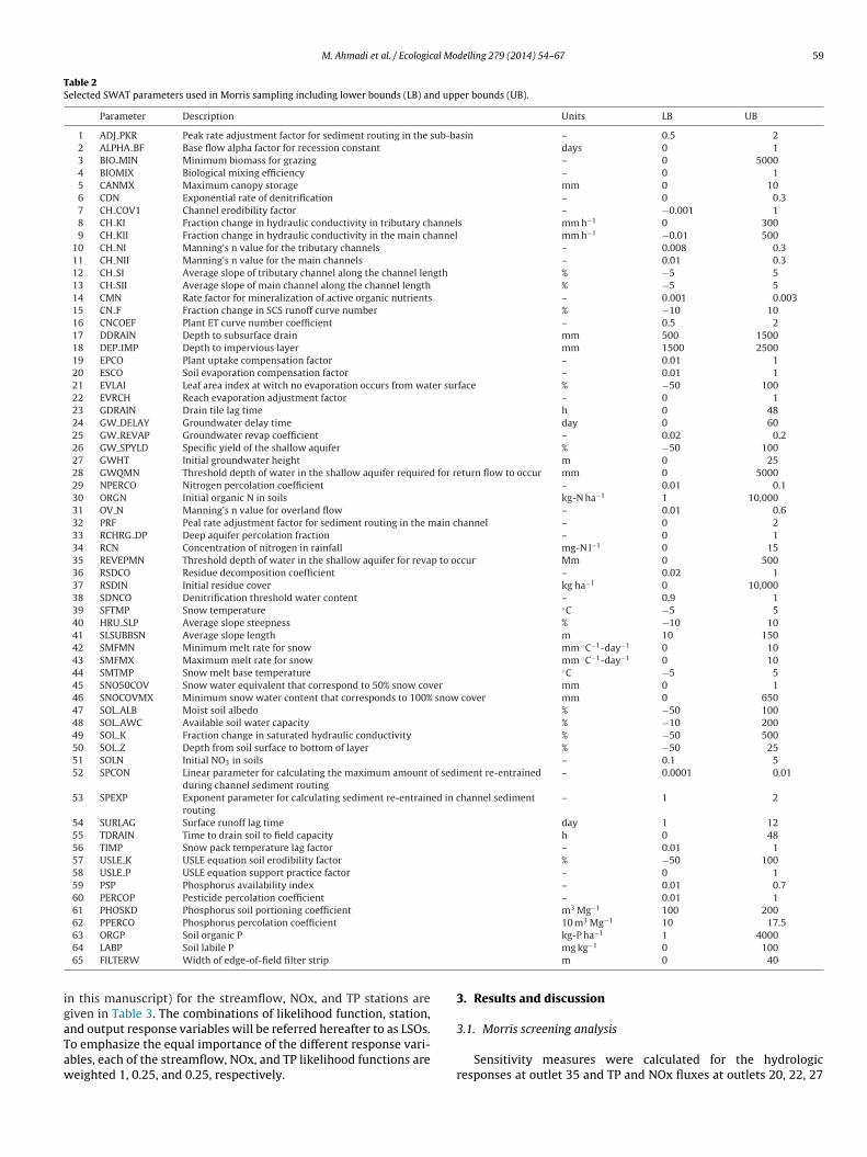

M. Ahmadi et al. / Ecological Modelling 279 (2014) 54–67 59

Table 2Selected SWAT parameters used in Morris sampling including lower bounds (LB) and upper bounds (UB).

Parameter Description Units LB UB

1 ADJ PKR Peak rate adjustment factor for sediment routing in the sub-basin – 0.5 22 ALPHA BF Base flow alpha factor for recession constant days 0 13 BIO MIN Minimum biomass for grazing – 0 50004 BIOMIX Biological mixing efficiency – 0 15 CANMX Maximum canopy storage mm 0 106 CDN Exponential rate of denitrification – 0 0.37 CH COV1 Channel erodibility factor – −0.001 18 CH KI Fraction change in hydraulic conductivity in tributary channels mm h−1 0 3009 CH KII Fraction change in hydraulic conductivity in the main channel mm h−1 −0.01 500

10 CH NI Manning’s n value for the tributary channels – 0.008 0.311 CH NII Manning’s n value for the main channels – 0.01 0.312 CH SI Average slope of tributary channel along the channel length % −5 513 CH SII Average slope of main channel along the channel length % −5 514 CMN Rate factor for mineralization of active organic nutrients – 0.001 0.00315 CN F Fraction change in SCS runoff curve number % −10 1016 CNCOEF Plant ET curve number coefficient – 0.5 217 DDRAIN Depth to subsurface drain mm 500 150018 DEP IMP Depth to impervious layer mm 1500 250019 EPCO Plant uptake compensation factor – 0.01 120 ESCO Soil evaporation compensation factor – 0.01 121 EVLAI Leaf area index at witch no evaporation occurs from water surface % −50 10022 EVRCH Reach evaporation adjustment factor – 0 123 GDRAIN Drain tile lag time h 0 4824 GW DELAY Groundwater delay time day 0 6025 GW REVAP Groundwater revap coefficient – 0.02 0.226 GW SPYLD Specific yield of the shallow aquifer % −50 10027 GWHT Initial groundwater height m 0 2528 GWQMN Threshold depth of water in the shallow aquifer required for return flow to occur mm 0 500029 NPERCO Nitrogen percolation coefficient – 0.01 0.130 ORGN Initial organic N in soils kg-N ha−1 1 10,00031 OV N Manning’s n value for overland flow – 0.01 0.632 PRF Peal rate adjustment factor for sediment routing in the main channel – 0 233 RCHRG DP Deep aquifer percolation fraction – 0 134 RCN Concentration of nitrogen in rainfall mg-N l−1 0 1535 REVEPMN Threshold depth of water in the shallow aquifer for revap to occur Mm 0 50036 RSDCO Residue decomposition coefficient – 0.02 137 RSDIN Initial residue cover kg ha−1 0 10,00038 SDNCO Denitrification threshold water content – 0.9 139 SFTMP Snow temperature ◦C −5 540 HRU SLP Average slope steepness % −10 1041 SLSUBBSN Average slope length m 10 15042 SMFMN Minimum melt rate for snow mm ◦C−1-day−1 0 1043 SMFMX Maximum melt rate for snow mm ◦C−1-day−1 0 1044 SMTMP Snow melt base temperature ◦C −5 545 SNO50COV Snow water equivalent that correspond to 50% snow cover mm 0 146 SNOCOVMX Minimum snow water content that corresponds to 100% snow cover mm 0 65047 SOL ALB Moist soil albedo % −50 10048 SOL AWC Available soil water capacity % −10 20049 SOL K Fraction change in saturated hydraulic conductivity % −50 50050 SOL Z Depth from soil surface to bottom of layer % −50 2551 SOLN Initial NO3 in soils – 0.1 552 SPCON Linear parameter for calculating the maximum amount of sediment re-entrained

during channel sediment routing– 0.0001 0.01

53 SPEXP Exponent parameter for calculating sediment re-entrained in channel sedimentrouting

– 1 2

54 SURLAG Surface runoff lag time day 1 1255 TDRAIN Time to drain soil to field capacity h 0 4856 TIMP Snow pack temperature lag factor – 0.01 157 USLE K USLE equation soil erodibility factor % −50 10058 USLE P USLE equation support practice factor – 0 159 PSP Phosphorus availability index – 0.01 0.760 PERCOP Pesticide percolation coefficient – 0.01 161 PHOSKD Phosphorus soil portioning coefficient m3 Mg−1 100 20062 PPERCO Phosphorus percolation coefficient 10 m3 Mg−1 10 17.5

−1

igaTaw

63 ORGP Soil organic P

64 LABP Soil labile P

65 FILTERW Width of edge-of-field filter strip

n this manuscript) for the streamflow, NOx, and TP stations areiven in Table 3. The combinations of likelihood function, station,

nd output response variables will be referred hereafter to as LSOs.o emphasize the equal importance of the different response vari-bles, each of the streamflow, NOx, and TP likelihood functions areeighted 1, 0.25, and 0.25, respectively.

kg-P ha 1 4000mg kg−1 0 100m 0 40

3. Results and discussion

3.1. Morris screening analysis

Sensitivity measures were calculated for the hydrologicresponses at outlet 35 and TP and NOx fluxes at outlets 20, 22, 27

60 M. Ahmadi et al. / Ecological Modelling 279 (2014) 54–67

Table 3List of informal likelihood functions and their corresponding reference numbers.

Output response Streamflow NOx TP

Station number 35 20 22 27 32 20 22 27 32

BIAS 1 5 9 13 17 21 25 29 33NSE 2 6 10 14 18 22 26 30 34PRMSE 3 7 11 15 19 23 27 31 35LRMSE 4 8 12 16 20 34 28 32 36

Table 4Top three most sensitive SWAT parameters, in order of corresponding rank, for all output responses and all informal likelihood functions evaluated. Numbers in parenthesesshow frequency (based on four informal likelihood functions for each variable at each station) of the parameter in the specified rank.

Output response Station Rank

1 2 3

Streamflow 35 ALPHA BF (4) CH KII (4) SOL K (2), ESCO (2)NOx 20 FILTERW (4) SOL Z, ORGN (2), SLSUBBSN SLSUBBSN, CDN (2), ESCONOx 22 FILTERW (4) SNO50COV, SLSUBBSN, RCN, CANMX SLSUBBSN (3), CANMXNOx 27 FILTERW (4) EPCO (2), CDN, RCN ESCO (2), RCN, CDNNOx 32 FILTERW (4) SNO50COV, RCN (3) CDN (2), SNO50COV, CN FTP 20 ALPHA BF (4) SLSUBBSN (3), CH NII PERCOP (2), CH KII, SLSUBBSNTP 22 ALPHA BF (3), SLSUBBSN SLSUBBSN (3), ALPHA BF CH KII (3), SNOCOVMXTP 27 ALPHA BF (3), CH NII SLSUBBSN (3), ALPHA BF PERCOP (2), CH KII, SLSUBBSNTP 32 ALPHA BF (4) SLSUBBSN (3), CH NII PERCOP (3), SLSUBBSN

Fig. 3. Morris sensitivity analysis results for all SWAT output responses. �* and � indicate the importance and degree of non-linearity or interaction caused by each parameter,respectively. Streamflow and nutrient units are m3 s−1 and kg ha−1 month, respectively.

al Modelling 279 (2014) 54–67 61

arsiSeasvrhfyC

aoh(tepFCts

eCU

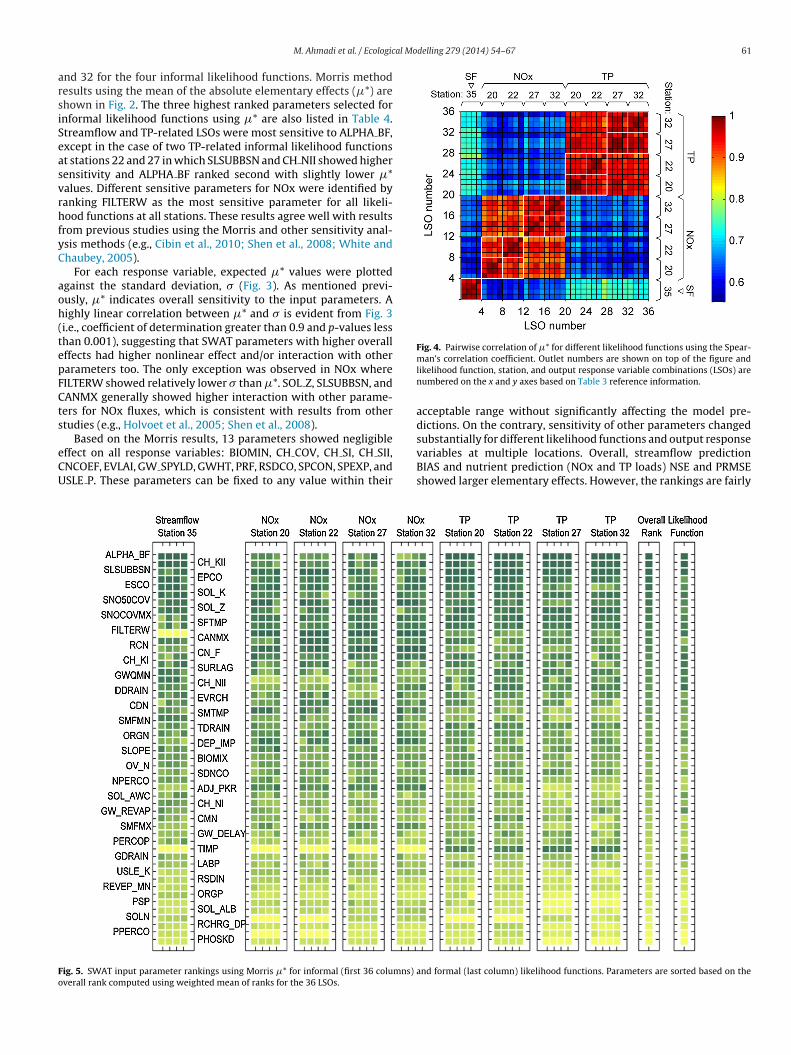
Fig. 4. Pairwise correlation of �* for different likelihood functions using the Spear-

Fo

M. Ahmadi et al. / Ecologic

nd 32 for the four informal likelihood functions. Morris methodesults using the mean of the absolute elementary effects (�*) arehown in Fig. 2. The three highest ranked parameters selected fornformal likelihood functions using �* are also listed in Table 4.treamflow and TP-related LSOs were most sensitive to ALPHA BF,xcept in the case of two TP-related informal likelihood functionst stations 22 and 27 in which SLSUBBSN and CH NII showed higherensitivity and ALPHA BF ranked second with slightly lower �*alues. Different sensitive parameters for NOx were identified byanking FILTERW as the most sensitive parameter for all likeli-ood functions at all stations. These results agree well with results

rom previous studies using the Morris and other sensitivity anal-sis methods (e.g., Cibin et al., 2010; Shen et al., 2008; White andhaubey, 2005).

For each response variable, expected �* values were plottedgainst the standard deviation, � (Fig. 3). As mentioned previ-usly, �* indicates overall sensitivity to the input parameters. Aighly linear correlation between �* and � is evident from Fig. 3i.e., coefficient of determination greater than 0.9 and p-values lesshan 0.001), suggesting that SWAT parameters with higher overallffects had higher nonlinear effect and/or interaction with otherarameters too. The only exception was observed in NOx whereILTERW showed relatively lower � than �*. SOL Z, SLSUBBSN, andANMX generally showed higher interaction with other parame-ers for NOx fluxes, which is consistent with results from othertudies (e.g., Holvoet et al., 2005; Shen et al., 2008).

Based on the Morris results, 13 parameters showed negligibleffect on all response variables: BIOMIN, CH COV, CH SI, CH SII,NCOEF, EVLAI, GW SPYLD, GWHT, PRF, RSDCO, SPCON, SPEXP, andSLE P. These parameters can be fixed to any value within their

ig. 5. SWAT input parameter rankings using Morris �* for informal (first 36 columns)

verall rank computed using weighted mean of ranks for the 36 LSOs.

man’s correlation coefficient. Outlet numbers are shown on top of the figure andlikelihood function, station, and output response variable combinations (LSOs) arenumbered on the x and y axes based on Table 3 reference information.

acceptable range without significantly affecting the model pre-dictions. On the contrary, sensitivity of other parameters changed

substantially for different likelihood functions and output responsevariables at multiple locations. Overall, streamflow predictionBIAS and nutrient prediction (NOx and TP loads) NSE and PRMSEshowed larger elementary effects. However, the rankings are fairly

and formal (last column) likelihood functions. Parameters are sorted based on the

62 M. Ahmadi et al. / Ecological Modelling 279 (2014) 54–67

Table 5Test of normality and homoscedasticity of model errors after implementing Box–Cox and AR(1) transformations.

Variable Location Normality tests Homoscedasticity tests

Chi-square p-value K-S p-value Bartlett’s p-value Levene’s p-value

Streamflow 35 0.000 0.158 0.333 0.002

NOx 20 0.216 0.985 0.869 0.56422 0.238 0.943 0.295 0.39127 0.384 0.975 0.807 0.21932 0.378 0.519 0.543 0.554

TP 20 0.400 0.713 0.975 0.94022 0.473 0.623 0.176 0.27927 0.870 0.998 0.974 0.35232 0.758 0.816 0.702 0.482

Table 6Transformation parameter values.

Response variable Outlet Lag − 1 coefficient (�) �v Box–Cox transformation parameter ( 1)

Streamflow 35 0.89 0.48 (m3 s−1) 0.06

NOx 20 0.35 0.98 (kg ha−1 month−1) 0.1222 0.14 0.87 (kg ha−1 month−1) 0.1227 0.26 0.87(kg ha−1 month−1) 0.1232 0.26 0.87(kg ha−1 month−1) 0.12

TP 20 0.54 2.30 (kg ha−1 month−1) 0.05.72 (kg ha−1 month−1) 0.05.41 (kg ha−1 month−1) 0.05.58 (kg ha−1 month−1) 0.05

cafiad

3

rSoofetls0mttip

ieflr2wcleec

0 10 20 30 40 50 600

10

20

30

40

50

60

Overall RankInformal Likelihood Function

For

mal

Lik

lihoo

d F

unct

ion

Ran

k

R2 = 0.91 p−value < 0.001

1:1 lineFitted Line

22 0.60 227 0.54 232 0.64 2

onsistent (Table 4 and Fig. 3), suggesting that different �* valuesre primarily due to differences in the units of likelihood functionsor the given model predictions and does not imply the relativemportance of the likelihood functions. Rank of parameters or Sav-ge scores are usually better means of comparing the results fromifferent methods and likelihood functions.

.2. Sensitivity indices correlation analysis

Pairwise correlation of �* for all 36 LSOs using Spearman’sank correlation coefficient (�) is illustrated in Fig. 4. A perfectpearman’s rank correlation coefficient of ±1 occurs when eachf the variables in one vector is a strictly monotone function of thether. A high correlation was evident between �* values of dif-erent likelihood functions of the same flux at each location. Forxample, Spearman’s rank correlation between likelihood func-ions of NOx was greater than 0.82 (p-value > 0.001) at differentocations. Correlation between different likelihood functions fortreamflow at station 35 and TP at four locations was greater than.9 (p-value > 0.001). Correlation between NSE and PRMSE wasore pronounced for all variables (r2 > 0.95) showing that NSE also

ends to emphasize high fluxes. LRMSE had the lowest correla-ion with other likelihood functions in all stations (all low as 0.81)mplying that the sensitive parameters for high and low fluxes areotentially different.

In addition to the existence of high correlation of sensitiv-ty measures between likelihood functions of the same fluxes atach location, sensitivity of likelihood functions of the similaruxes at multiple locations were also highly correlated. The cor-elation was stronger between upstream stations (stations 20 and2 in Fig. 1), and also between downstream stations close to theatershed outlet (stations 27 and 32 in Fig. 1). Similarly, high

orrelation between TP-related likelihood functions at different

ocations was noticeable and can be attributed to the hydrologicvent-driven nature of TP transport. Although discrete hydrologicvents strongly impact NOx mobilization, biogeochemical pro-esses of nitrogen are highly dependent on land-use/land-cover,

Fig. 6. Correlation between SWAT input parameter rankings for the formal andinformal likelihood functions.

management practices, fertilizer application, groundwater flow,and other environmental conditions that may occur throughoutthe year. Correlation between sensitivity measures at the nestedoutlet stations (22 and 27) was also higher than for other stations.This correlation was stronger for TP. Overall, BIAS and LRMSE hadthe lowest correlation with other likelihood functions at differentstations.

Despite the high correlation between similar output response

variables at multiple locations, there was lower correlationbetween sensitivity measures of different fluxes as indicated by theblue (correlation < 0.7) in Fig. 4. NOx fluxes showed the lowest cor-relation with streamflow and TP fluxes, with the lowest correlation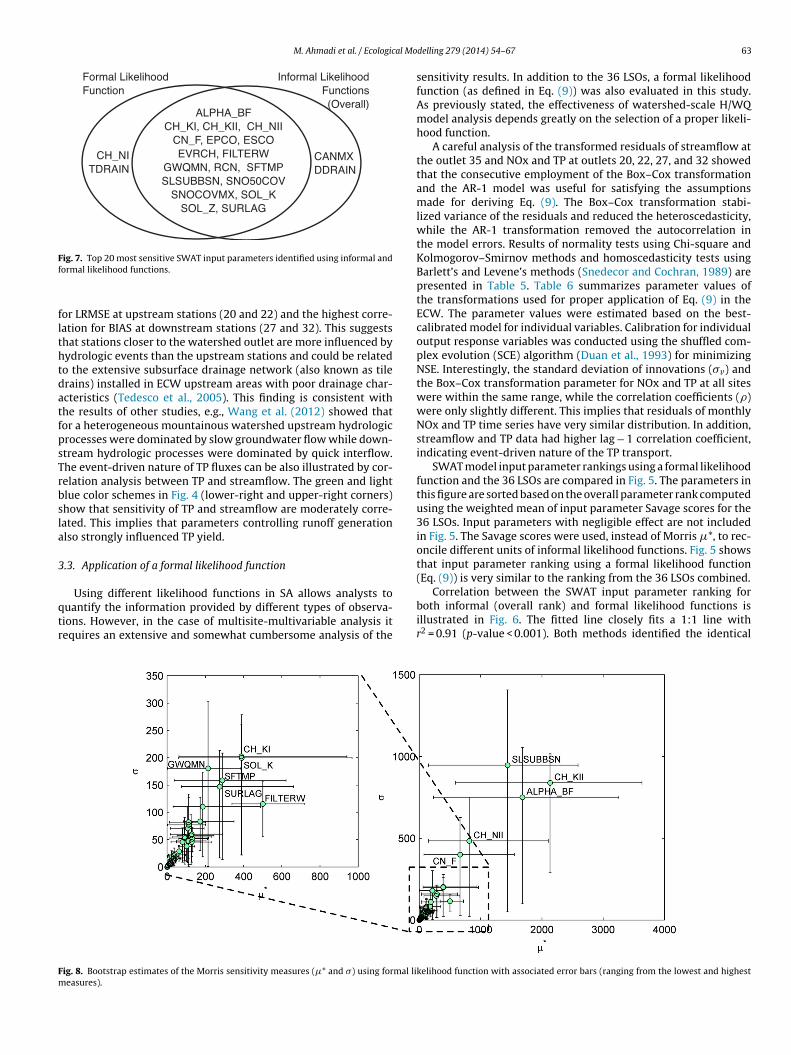

M. Ahmadi et al. / Ecological Mo

Ff

flthtdatfpsTrbsla

3

qtr

Fm

ig. 7. Top 20 most sensitive SWAT input parameters identified using informal andormal likelihood functions.

or LRMSE at upstream stations (20 and 22) and the highest corre-ation for BIAS at downstream stations (27 and 32). This suggestshat stations closer to the watershed outlet are more influenced byydrologic events than the upstream stations and could be relatedo the extensive subsurface drainage network (also known as tilerains) installed in ECW upstream areas with poor drainage char-cteristics (Tedesco et al., 2005). This finding is consistent withhe results of other studies, e.g., Wang et al. (2012) showed thator a heterogeneous mountainous watershed upstream hydrologicrocesses were dominated by slow groundwater flow while down-tream hydrologic processes were dominated by quick interflow.he event-driven nature of TP fluxes can be also illustrated by cor-elation analysis between TP and streamflow. The green and lightlue color schemes in Fig. 4 (lower-right and upper-right corners)how that sensitivity of TP and streamflow are moderately corre-ated. This implies that parameters controlling runoff generationlso strongly influenced TP yield.

.3. Application of a formal likelihood function

Using different likelihood functions in SA allows analysts touantify the information provided by different types of observa-ions. However, in the case of multisite-multivariable analysis itequires an extensive and somewhat cumbersome analysis of the

ig. 8. Bootstrap estimates of the Morris sensitivity measures (�* and �) using formal lieasures).

delling 279 (2014) 54–67 63

sensitivity results. In addition to the 36 LSOs, a formal likelihoodfunction (as defined in Eq. (9)) was also evaluated in this study.As previously stated, the effectiveness of watershed-scale H/WQmodel analysis depends greatly on the selection of a proper likeli-hood function.

A careful analysis of the transformed residuals of streamflow atthe outlet 35 and NOx and TP at outlets 20, 22, 27, and 32 showedthat the consecutive employment of the Box–Cox transformationand the AR-1 model was useful for satisfying the assumptionsmade for deriving Eq. (9). The Box–Cox transformation stabi-lized variance of the residuals and reduced the heteroscedasticity,while the AR-1 transformation removed the autocorrelation inthe model errors. Results of normality tests using Chi-square andKolmogorov–Smirnov methods and homoscedasticity tests usingBarlett’s and Levene’s methods (Snedecor and Cochran, 1989) arepresented in Table 5. Table 6 summarizes parameter values ofthe transformations used for proper application of Eq. (9) in theECW. The parameter values were estimated based on the best-calibrated model for individual variables. Calibration for individualoutput response variables was conducted using the shuffled com-plex evolution (SCE) algorithm (Duan et al., 1993) for minimizingNSE. Interestingly, the standard deviation of innovations (�v) andthe Box–Cox transformation parameter for NOx and TP at all siteswere within the same range, while the correlation coefficients (�)were only slightly different. This implies that residuals of monthlyNOx and TP time series have very similar distribution. In addition,streamflow and TP data had higher lag − 1 correlation coefficient,indicating event-driven nature of the TP transport.

SWAT model input parameter rankings using a formal likelihoodfunction and the 36 LSOs are compared in Fig. 5. The parameters inthis figure are sorted based on the overall parameter rank computedusing the weighted mean of input parameter Savage scores for the36 LSOs. Input parameters with negligible effect are not includedin Fig. 5. The Savage scores were used, instead of Morris �*, to rec-oncile different units of informal likelihood functions. Fig. 5 showsthat input parameter ranking using a formal likelihood function(Eq. (9)) is very similar to the ranking from the 36 LSOs combined.

Correlation between the SWAT input parameter ranking forboth informal (overall rank) and formal likelihood functions isillustrated in Fig. 6. The fitted line closely fits a 1:1 line withr2 = 0.91 (p-value < 0.001). Both methods identified the identical

kelihood function with associated error bars (ranging from the lowest and highest

64 M. Ahmadi et al. / Ecological Modelling 279 (2014) 54–67

Table 7SWAT parameter rankings for informal and formal likelihood functions and lower and upper ranks using �* from the bootstrap replica.

Parameter Overall rank (informal likelihood function) Formal likelihood function rank

Baseline Lower rank Upper rank Baseline Lower rank Upper rank

1 ADJ PKR 32 24 38 21 15 272 ALPHA BF 1 1 7 2 1 83 BIO MIN 53 53 53 53 53 534 BIOMIX 28 27 34 36 30 395 CANMX 12 10 18 31 27 376 CDN 21 14 24 24 18 297 CH COV1 53 53 53 53 53 538 CH KI 15 8 22 7 4 139 CH KII 2 2 8 1 1 3

10 CH NI 34 28 38 16 12 2211 CH NII 18 12 17 4 2 1012 CH SI 53 53 53 53 53 5313 CH SII 53 53 53 53 53 5314 CMN 36 29 39 34 28 3815 CN F 14 8 12 5 3 1116 CNCOEF 53 53 53 53 53 5317 DDRAIN 19 13 23 25 19 3018 DEP IMP 26 20 29 32 24 3819 EPCO 4 2 10 20 14 2720 ESCO 5 2 11 14 8 2021 EVLAI 53 53 53 53 53 5322 EVRCH 20 14 26 18 10 2423 GDRAIN 41 34 41 33 25 4124 GW DELAY 38 30 44 41 37 4725 GW REVAP 35 29 42 40 37 4726 GW SPYLD 53 53 53 53 53 5327 GWHT 53 53 53 53 53 5328 GWQMN 17 10 23 11 5 1729 NPERCO 31 29 37 37 31 4030 ORGN 25 17 24 22 16 2531 OV N 29 23 31 23 17 2932 PRF 53 53 53 53 53 5333 RCHRG DP 50 50 53 52 49 5334 RCN 13 13 19 15 10 2135 REVEPMN 45 41 53 48 44 5336 RSDCO 53 53 53 53 53 5337 RSDIN 44 40 46 42 40 4938 SDNCO 30 28 38 39 33 4139 SFTMP 10 5 16 9 6 1540 HRU SLP 27 22 35 28 22 3441 SLSUBBSN 3 1 7 3 1 942 SMFMN 23 19 29 29 23 3643 SMFMX 37 33 41 35 29 4144 SMTMP 22 17 28 26 20 3245 SNO50COV 7 2 13 13 8 1946 SNOCOVMX 9 6 15 12 7 1847 SOL ALB 48 45 49 45 41 4948 SOL AWC 33 28 39 30 22 3649 SOL K 6 2 12 8 4 1450 SOL Z 8 3 11 17 11 2351 SOLN 49 45 49 47 41 4952 SPCON 53 53 53 53 53 5353 SPEXP 53 53 53 53 53 5354 SURLAG 16 12 22 10 7 1655 TDRAIN 24 18 30 19 13 2556 TIMP 40 34 38 27 21 3557 USLE K 43 41 46 43 41 4758 USLE P 53 53 53 53 53 5359 PSP 47 43 46 46 40 4760 PERCOP 39 33 39 38 32 3961 PHOSKD 52 48 52 50 48 5262 PPERCO 51 47 52 51 49 5263 ORGP 46 44 51 49 45 5164 LABP 42 41 48 44 41 48

1

naTtp

65 FILTERW 11 8

egligible parameters (i.e., 13 out of 65 parameters with zero mean

nd standard deviation) and very similar less sensitive parameters.he top 20 most sensitive SWAT input parameters identified byhe two approaches are depicted in Fig. 7, in which 18 similararameters were recognized to be important by both methods.

4 6 3 11

3.4. Sensitivity indices uncertainty analysis: bootstrapping

The Morris GSA results can be refined based on bootstrapreplicates to analyze robustness of the results and make strongerdistinctions between parameter effects. Fig. 8 shows the Morris

M. Ahmadi et al. / Ecological Mo

Ff

meifmaeFil

fflabnaloofs

mstssN

4

dtFn

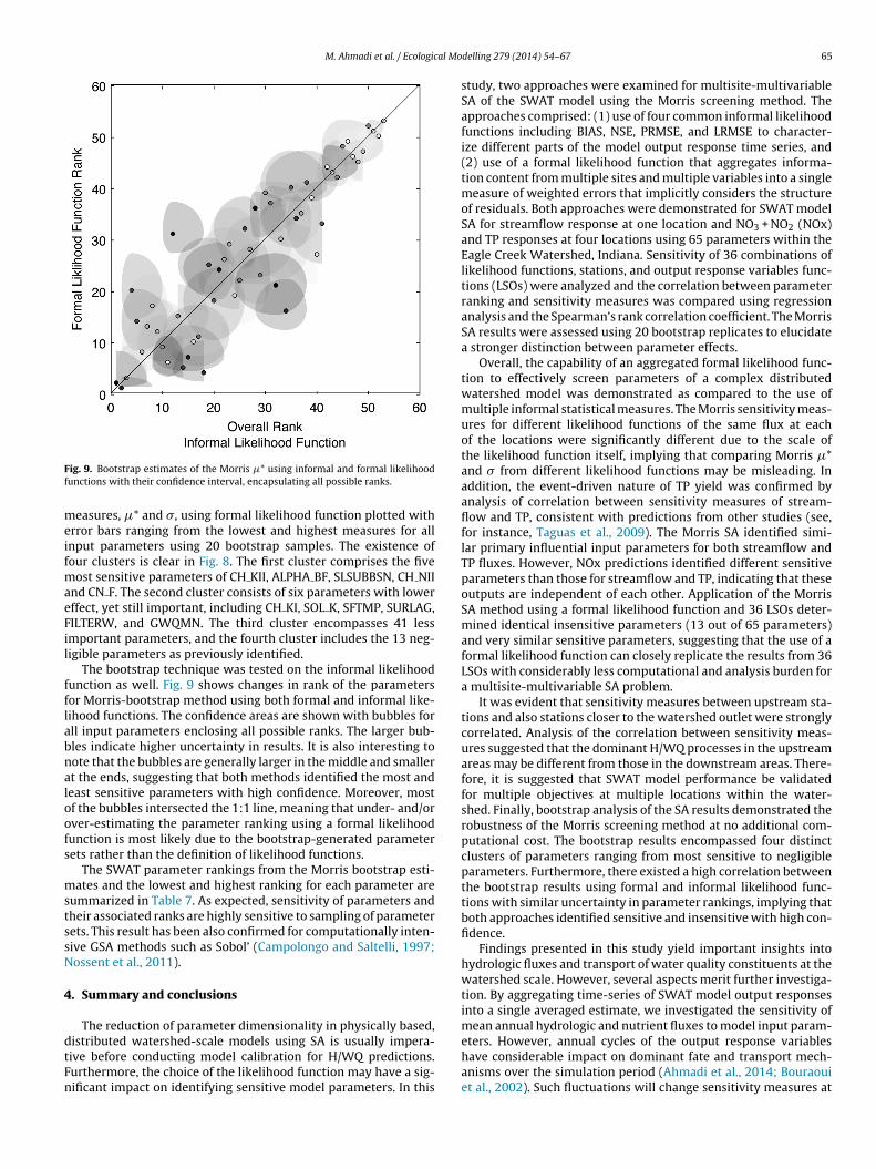
ig. 9. Bootstrap estimates of the Morris �* using informal and formal likelihoodunctions with their confidence interval, encapsulating all possible ranks.

easures, �* and �, using formal likelihood function plotted withrror bars ranging from the lowest and highest measures for allnput parameters using 20 bootstrap samples. The existence ofour clusters is clear in Fig. 8. The first cluster comprises the five

ost sensitive parameters of CH KII, ALPHA BF, SLSUBBSN, CH NIInd CN F. The second cluster consists of six parameters with lowerffect, yet still important, including CH KI, SOL K, SFTMP, SURLAG,ILTERW, and GWQMN. The third cluster encompasses 41 lessmportant parameters, and the fourth cluster includes the 13 neg-igible parameters as previously identified.

The bootstrap technique was tested on the informal likelihoodunction as well. Fig. 9 shows changes in rank of the parametersor Morris-bootstrap method using both formal and informal like-ihood functions. The confidence areas are shown with bubbles forll input parameters enclosing all possible ranks. The larger bub-les indicate higher uncertainty in results. It is also interesting toote that the bubbles are generally larger in the middle and smallert the ends, suggesting that both methods identified the most andeast sensitive parameters with high confidence. Moreover, mostf the bubbles intersected the 1:1 line, meaning that under- and/orver-estimating the parameter ranking using a formal likelihoodunction is most likely due to the bootstrap-generated parameterets rather than the definition of likelihood functions.

The SWAT parameter rankings from the Morris bootstrap esti-ates and the lowest and highest ranking for each parameter are

ummarized in Table 7. As expected, sensitivity of parameters andheir associated ranks are highly sensitive to sampling of parameterets. This result has been also confirmed for computationally inten-ive GSA methods such as Sobol’ (Campolongo and Saltelli, 1997;ossent et al., 2011).

. Summary and conclusions

The reduction of parameter dimensionality in physically based,

istributed watershed-scale models using SA is usually impera-ive before conducting model calibration for H/WQ predictions.urthermore, the choice of the likelihood function may have a sig-ificant impact on identifying sensitive model parameters. In this

delling 279 (2014) 54–67 65

study, two approaches were examined for multisite-multivariableSA of the SWAT model using the Morris screening method. Theapproaches comprised: (1) use of four common informal likelihoodfunctions including BIAS, NSE, PRMSE, and LRMSE to character-ize different parts of the model output response time series, and(2) use of a formal likelihood function that aggregates informa-tion content from multiple sites and multiple variables into a singlemeasure of weighted errors that implicitly considers the structureof residuals. Both approaches were demonstrated for SWAT modelSA for streamflow response at one location and NO3 + NO2 (NOx)and TP responses at four locations using 65 parameters within theEagle Creek Watershed, Indiana. Sensitivity of 36 combinations oflikelihood functions, stations, and output response variables func-tions (LSOs) were analyzed and the correlation between parameterranking and sensitivity measures was compared using regressionanalysis and the Spearman’s rank correlation coefficient. The MorrisSA results were assessed using 20 bootstrap replicates to elucidatea stronger distinction between parameter effects.

Overall, the capability of an aggregated formal likelihood func-tion to effectively screen parameters of a complex distributedwatershed model was demonstrated as compared to the use ofmultiple informal statistical measures. The Morris sensitivity meas-ures for different likelihood functions of the same flux at eachof the locations were significantly different due to the scale ofthe likelihood function itself, implying that comparing Morris �*and � from different likelihood functions may be misleading. Inaddition, the event-driven nature of TP yield was confirmed byanalysis of correlation between sensitivity measures of stream-flow and TP, consistent with predictions from other studies (see,for instance, Taguas et al., 2009). The Morris SA identified simi-lar primary influential input parameters for both streamflow andTP fluxes. However, NOx predictions identified different sensitiveparameters than those for streamflow and TP, indicating that theseoutputs are independent of each other. Application of the MorrisSA method using a formal likelihood function and 36 LSOs deter-mined identical insensitive parameters (13 out of 65 parameters)and very similar sensitive parameters, suggesting that the use of aformal likelihood function can closely replicate the results from 36LSOs with considerably less computational and analysis burden fora multisite-multivariable SA problem.

It was evident that sensitivity measures between upstream sta-tions and also stations closer to the watershed outlet were stronglycorrelated. Analysis of the correlation between sensitivity meas-ures suggested that the dominant H/WQ processes in the upstreamareas may be different from those in the downstream areas. There-fore, it is suggested that SWAT model performance be validatedfor multiple objectives at multiple locations within the water-shed. Finally, bootstrap analysis of the SA results demonstrated therobustness of the Morris screening method at no additional com-putational cost. The bootstrap results encompassed four distinctclusters of parameters ranging from most sensitive to negligibleparameters. Furthermore, there existed a high correlation betweenthe bootstrap results using formal and informal likelihood func-tions with similar uncertainty in parameter rankings, implying thatboth approaches identified sensitive and insensitive with high con-fidence.

Findings presented in this study yield important insights intohydrologic fluxes and transport of water quality constituents at thewatershed scale. However, several aspects merit further investiga-tion. By aggregating time-series of SWAT model output responsesinto a single averaged estimate, we investigated the sensitivity ofmean annual hydrologic and nutrient fluxes to model input param-

eters. However, annual cycles of the output response variableshave considerable impact on dominant fate and transport mech-anisms over the simulation period (Ahmadi et al., 2014; Bouraouiet al., 2002). Such fluctuations will change sensitivity measures at

6 al Mo

dlrilsabnmcdsbftw

A

N0

R

A

A

A

A

A

A

A

B

B

B

B

B

B

B

B

C

6 M. Ahmadi et al. / Ecologic

ifferent time periods. Investigation of temporal changes for hydro-ogic and nutrient fluxes may yield insights into how sensitivity ofesponses and interaction between different processes may changen different seasons. Additionally, our analysis was performed atocations within the stream network that fully encompassed in-tream and overland processes from upstream areas. Sensitivitynalysis of the overland fluxes of water and nutrients may provideetter understanding of the processes controlling transport mecha-isms at different spatial scales. Also, application of an event-basedodel may yield enhanced perception of the governing processes

ontrolling transport of phosphorus. Moreover, the impact of theistance between sites on correlation of the sensitivity measureshould be further investigated. Finally, analysis of the correlationetween sensitivity of sediment fluxes and dissolved or particulateorms of nutrients may result in a better understanding of the rela-ionship between sediment delivery and nutrient transport at theatershed scale.

cknowledgment

This study was funded by U.S. Department of Agriculture-ational Institute of Food and Agriculture grants 2007-51130-3876 and 2009-51130-06038.

eferences

hmadi, M., 2012. A multi criteria decision support system for watershed manage-ment under uncertain conditions. Colorado State University, Fort Collins, CO(Unpublished Ph.D. Dissertation).

hmadi, M., Records, R., Arabi, M., 2014. Impact of climate change on diffusepollutant fluxes at the watershed scale. Hydrologic Processes 28, 1962–1972,http://dx.doi.org/10.1002/hyp.9723.

jami, N.K., Duan, Q., Sorooshian, S., 2007. An integrated hydrologic Bayesian mul-timodel combination framework: confronting input, parameter, and modelstructural uncertainty in hydrologic prediction. Water Resources Research 43(1), http://dx.doi.org/10.1029/2005WR004745.

rabi, M., Govindaraju, R.S., Engel, B.A., Hantush, M.M., 2007. Multiobjective sen-sitivity analysis of sediment and nitrogen processes with a watershed model.Water Resources Research 43 (6), http://dx.doi.org/10.1029/2006WR005463.

rnold, J.G., Kiniry, J.R., Srinivasan, R., Williams, J.R., Haney, E.B., Neitsch, S.L., 2012.Soil and Water Assessment Tool Input/Output File Documentation, Version2009, Report No. 365. Technical report, Texas Water Resources Institute, CollegeStation, TX.

ronica, G., Hankin, B., Beven, K., 1998. Uncertainty and equifinality incalibrating distributed roughness coefficients in a flood propagationmodel with limited data. Advances in Water Resources 22 (4), 349–365,http://dx.doi.org/10.1016/S0309-1708(98)00017-7.

SCE, 1993. Criteria for evaluation of watershed models, ASCE task committee ondefinition of criteria for evaluation of watershed models of the watershed man-agement, irrigation, and drainage division. Journal of Irrigation and DrainageEngineering 119 (3), 429.

even, K., Binley, A., 1992. The future of distributed models: model calibra-tion and uncertainty prediction. Hydrological Processes 6 (3), 279–298,http://dx.doi.org/10.1002/hyp.3360060305.

even, K., Freer, J., 2001. Equifinality, data assimilation, and uncertaintyestimation in mechanistic modelling of complex environmental systemsusing the GLUE methodology. Journal of Hydrology 249 (1–4), 11–29,http://dx.doi.org/10.1016/S0022-1694(01)00421-8.

ouraoui, F., Galbiati, L., Bidoglio, G., 2002. Climate change impacts on nutrient loadsin the Yorkshire Ouse catchment (UK). Hydrology and Earth System Sciences 6,197–209, http://dx.doi.org/10.5194/hess-6-197-2002.

ox, G.E.P., Cox, D., 1964. An analysis of transformations. Journal of the Royal Statis-tical Society, Series B 26, 1–78.

ox, G.E.P., Tiao, G.C., 1992. Bayesian Inference in Statistical Analysis. John Wiley &Sons, Inc., New York, NY.

ox, G.E.P., Jenkins, G.M., Reinsel, G.C., 2008. Time Series Analysis: Forecasting andControl, 4th ed. John Wiley & Sons, Inc., New York, NY.

rockmann, D., Morgenroth, E., 2007. Comparing global sensitivity analysis for abiofilm model for two-step nitrification using the qualitative screening methodof Morris or the quantitative variance-based Fourier Amplitude Sensitivity Test(FAST). Water Science and Technology 56 (8), 85–93.

rown, L.C., Barnwell, T.O., 1987. The enhanced water quality models QUAL2E andQUAL2E-UNCAS documentation and user manual. Technical report, EPA docu-ment EPA/600/3-87/007. USEPA, Athens, GA.

acuci, D.G., 2003. Sensitivity and Uncertainty Analysis, Volume I: Theory. CRC Press,Boca Raton, Florida.

delling 279 (2014) 54–67

Cacuci, D.G., Ionescu-bujor, M., 2004. A comparative review of sensitivity and uncer-tainty analysis of large-scale systems. II: Statistical methods. Nuclear Scienceand Engineering 147 (3), 204–217.

Campolongo, F., Saltelli, A., 1997. Sensitivity analysis of an environmental model:an application of different analysis methods. Reliability Engineering and SystemSafety 57 (1), 49–69, http://dx.doi.org/10.1016/S0951-8320(97)00021-5.

Campolongo, F., Braddock, R., 1999. Sensitivity analysis of the IMAGE Green-house model. Environmental Modelling & Software 14 (4), 275–282,http://dx.doi.org/10.1016/S1364-8152(98)00079-6.

Campolongo, F., Cariboni, J., Saltelli, A., 2007. An effective screening design for sensi-tivity analysis of large models. Environmental Modelling and Software 22 (10),1509–1518, http://dx.doi.org/10.1016/j.envsoft.2006.10.004.

Cibin, R., Sudheer, K.P., Chaubey, I., 2010. Sensitivity and identifiability of streamflow generation parameters of the SWAT model. Hydrological Processes 24 (9),1133–1148, http://dx.doi.org/10.1002/hyp.7568.

Ciric, C., Ciffroy, P., Charles, S., 2012. Use of sensitivity analysis to identify influentialand non-influential parameters within an aquatic ecosystem model. EcologicalModelling 246, 119–130, http://dx.doi.org/10.1016/j.ecolmodel.2012.06.024.

Confalonieri, R., Bellocchi, G., Donatelli, M., 2010. A software component to computeagro-meteorological indicators. Environmental Modelling and Software 25 (11),1485–1486, http://dx.doi.org/10.1016/j.envsoft.2008.11.007.

Cotter, A.S., Chaubey, I., Costello, T.A., Soerens, T.S., Nelson, M.A., 2003. Waterquality model output uncertainty as affected by spatial resolution of inputdata. Journal of the American Water Resources Association 39 (4), 977–986,http://dx.doi.org/10.1111/j.1752-1688.2003.tb04420.x.

DeJonge, K.C., Ascough II, J.C., Ahmadi, M., Andales, A.A., Arabi, M., 2012. Globalsensitivity and uncertainty analysis of a dynamic agroecosystem modelunder different irrigation treatments. Ecological Modelling 231, 113–125,http://dx.doi.org/10.1016/j.ecolmodel.2012.01.024.

DiToro, D., 1984. Statistical methods for estimating and evaluating the uncertainty ofwater quality model parameters and predictions. Technical report, ManhattanCollege, Prepared for the Delft Hydraulics Laboratory, Delft, The Netherlands,Bronx, NY.

Duan, Q., Gupta, V.K., Sorooshian, S., 1993. Shuffled complex evolution approach foreffective and efficient global minimization. Journal of Optimization Theory andApplications 76 (3), 501–521, http://dx.doi.org/10.1007/BF00939380.

Efron, B., 1979. Bootstrap methods: another look at the Jackknife. Annals of Statistics7 (1), 1–26.

Fenicia, F., Savenije, H.H.G., Matgen, P., Pfister, L., 2007. A comparison of alter-native multiobjective calibration strategies for hydrological modeling. WaterResources Research 43 (3), http://dx.doi.org/10.1029/2006WR005098.

Feyereisen, G., Strickland, T., Bosch, D., 2007. Evaluation of SWAT manual calibrationand input parameter sensitivity in the Little River Watershed. Transactions ofthe ASABE 50, 843–856.

Foglia, L., Hill, M.C., Mehl, S.W., Burlando, P., 2009. Sensitivity analysis, cali-bration, and testing of a distributed hydrological model using error-basedweighting and one objective function. Water Resources Research 45 (6),http://dx.doi.org/10.1029/2008WR007255.

Francos, A., Elorza, F., Bouraoui, F., Bidoglio, G., Galbiati, L., 2003. Sensi-tivity analysis of distributed environmental simulation models: under-standing the model behaviour in hydrological studies at the catch-ment scale. Reliability Engineering and System Safety 79 (2), 205–218,http://dx.doi.org/10.1016/S0951-8320(02)00231-4.

Gupta, H.V., Sorooshian, S., Yapo, P.O., 1999. Status of automatic cali-bration for hydrologic models: comparison with multilevel expertcalibration. Journal of Hydrologic Engineering 4 (2), 135–143,http://dx.doi.org/10.1061/(ASCE)1084-0699(1999)4:2(135).

Haan, C.T., Storm, D.E., Al-Issa, T., Prabhu, S., Sabbagh, G.J., Edwards, D.R., 1998.Effect of parameter distributions on uncertainty analysis of hydrologic models.Transactions of the ASAE 41 (1), 65–70.

Hall, J.W., Boyce, S.A., Wang, Y., Dawson, R.J., Tarantola, S., Saltelli, A., 2009. Sensi-tivity analysis for hydraulic models. Journal of Hydraulic Engineering 135 (11),959, http://dx.doi.org/10.1061/(ASCE)HY.1943-7900.0000098.

He, J., Jones, J.W., Graham, W.D., Dukes, M.D., 2010. Influence of likelihood functionchoice for estimating crop model parameters using the generalized likeli-hood uncertainty estimation method. Agricultural Systems 103 (5), 256–264,http://dx.doi.org/10.1016/j.agsy.2010.01.006.

Helton, J.C., 2008. Uncertainty and sensitivity analysis for models of complex sys-tems. In: Graziani, F. (Ed.), Computational Methods in Transport: Verificationand Validation, Volume 62 of Lecture Notes in Computational Science and Engi-neering. Springer, Berlin/Heidelberg, pp. 207–228.

Holvoet, K., van Griensven, A., Seuntjens, P., Vanrolleghem, P., 2005. Sensi-tivity analysis for hydrology and pesticide supply towards the river inSWAT. Physics and Chemistry of the Earth, Parts A/B/C 30 (8–10), 518–526,http://dx.doi.org/10.1016/j.pce.2005.07.006.

Huang, Y., Liu, L., 2008. A hybrid perturbation and Morris approach for identifyingsensitive parameters in surface water quality models. Journal of EnvironmentalInformatics 12 (2), 150–159, http://dx.doi.org/10.3808/jei.200800133.

Iman, R.L., Conover, W.J., 1987. A measure of top-down correlation. Technometrics29 (3), 351.

King, D., Perera, B., 2013. Morris method of sensitivity analysis applied to assess the

importance of input variables on urban water supply yield – a case study. Journalof Hydrology 477, 17–32, http://dx.doi.org/10.1016/j.jhydrol.2012.10.017.

Kuczera, G., Parent, E., 1998. Monte Carlo assessment of parameter uncertainty inconceptual catchment models: the Metropolis algorithm. Journal of Hydrology211 (1–4), 69–85, http://dx.doi.org/10.1016/S0022-1694(98)00198-X.

al Mo

M

M

M

M

M

M

M

N

N

P

R

S

S

S

S

S

S

S

S

S

S

T

297–316.

M. Ahmadi et al. / Ecologic

adsen, H., 2000. Automatic calibration of a conceptual rainfall runoff modelusing multiple objectives. Journal of Hydrology 235 (3–4), 276–288,http://dx.doi.org/10.1016/S0022-1694(00)00279-1.

adsen, H., 2003. Parameter estimation in distributed hydrological catchment mod-elling using automatic calibration with multiple objectives. Advances in WaterResources 26 (2), 205–216, http://dx.doi.org/10.1016/S0309-1708(02)00092-1.

antovan, P., Todini, E., 2006. Hydrological forecasting uncertainty assessment:incoherence of the GLUE methodology. Journal of Hydrology 330 (1–2), 368–381,http://dx.doi.org/10.1016/j.jhydrol.2006.04.046.

onod, H., Naud, C., Makowski, D., 2006. Uncertainty and sensitivity analysis for cropmodels. In: Wallach, D., Makowski, D., Jones, J. (Eds.), Working with DynamicCrop Models. Elsevier Science, Amsterdam, the Netherlands, pp. 55–100.

oriasi, D.N., Arnold, J.G., Van Liew, M.W., Bingner, R.L., Harmel, R.D., Veith, T.L.,2007. Model evaluation guidelines for systematic quantification of accuracy inwatershed simulations. Transactions of the ASABE 50 (3), 885–900.

orris, M., 1991. Factorial sampling plans for preliminary computational experi-ments. Technometrics 33 (2), 161–174.

uleta, M.K., Nicklow, J.W., 2005. Sensitivity and uncertainty analysis coupled withautomatic calibration for a distributed watershed model. Journal of Hydrology306 (1–4), 127–145, http://dx.doi.org/10.1016/j.jhydrol.2004.09.005.

ash, J.E., Sutcliffe, J., 1970. River flow forecasting through conceptual mod-els. Part I: A discussion of principles. Journal of Hydrology 10 (3), 282–290,http://dx.doi.org/10.1016/0022-1694(70)90255-6.

ossent, J., Elsen, P., Bauwens, W., 2011. Sobol sensitivity analysis of a complex envi-ronmental model. Environmental Modelling and Software 26 (12), 1515–1525,http://dx.doi.org/10.1016/j.envsoft.2011.08.010.

appenberger, F., Beven, K.J., Ratto, M., Matgen, P., 2008. Multi-method global sensi-tivity analysis of flood inundation models. Advances in Water Resources 31 (1),1–14, http://dx.doi.org/10.1016/j.advwatres.2007.04.009.

unkel, R., Crawford, C., Cohn, T., 2004. Load estimator (LOADEST): a FORTRAN pro-gram for estimating constituent loads in streams and rivers. In: U.S. GeologicalSurvey Techniques and Methods Book 4. U.S. Geological Survey, pp. 69 (ChapterA5).

altelli, A., Tarantola, S., Chan, K.P.-S., 1999. A quantitative model-independentmethod for global sensitivity analysis of model output. Technometrics 41 (1),39.

altelli, A., Chan, K., Scott, E.M., 2000. Sensitivity Analysis. John Wiley and Sons, Ltd.,West Sussex, UK.

altelli, A., Tarantola, S., Campolongo, F., Ratto, M., 2004. Sensitivity Analysis inPractice: A Guide to Assessing Scientific Models, 1st ed. John Wiley and Sons,Ltd., West Sussex UK.

altelli, A., Ratto, M., Tarantola, S., Campolongo, F., 2006. Sensitivity analysis prac-tices: strategies for model-based inference. Reliability Engineering and SystemSafety 91 (10–11), 1109–1125, http://dx.doi.org/10.1016/j.ress.2005.11.014.

altelli, A., Ratto, M., Andres, T., Campolongo, F., Cariboni, J., Gatelli, D., Saisana, M.,Tarantola, S., 2008. Global Sensitivity Analysis: The Primer. John Wiley and Sons,Ltd., West Sussex, UK.

hen, Z., Hong, Q., Yu, H., Liu, R., 2008. Parameter uncertainty analysis of the non-point source pollution in the Daning River watershed of the Three GorgesReservoir Region, China. Science of the Total Environment 405 (1–3), 195–205,http://dx.doi.org/10.1016/j.scitotenv.2008.06.009.

nedecor, G.W., Cochran, W.G., 1989. Statistical Methods. Iowa State UniversityPress, Ames, IA, pp. 503.

orooshian, S., Dracup, J.A., 1980. Stochastic parameter estimation proceduresfor hydrologie rainfall-runoff models: correlated and heteroscedastic errorcases. Water Resources Research 16 (2), 430–442, http://dx.doi.org/10.1029/WR016i002p00430.

tedinger, J.R., Vogel, R.M., Lee, S.U., Batchelder, R., 2008. Appraisal of the generalizedlikelihood uncertainty estimation (GLUE) method. Water Resources Research 44,http://dx.doi.org/10.1029/2008WR006822.

un, X., Newham, L., Croke, B., Norton, J., 2012. Three complementary methodsfor sensitivity analysis of a water quality model. Environmental Modelling andSoftware 37, 19–29, http://dx.doi.org/10.1016/j.envsoft.2012.04.010.

aguas, E.V., Ayuso, J.L., Pena, A., Yuan, Y., Pérez, R., 2009. Evaluating and modellingthe hydrological and erosive behaviour of an olive orchard microcatchment

delling 279 (2014) 54–67 67

under no-tillage with bare soil in Spain. Earth Surface Processes and Landforms34, 738–751, http://dx.doi.org/10.1002/esp.1775.

Tedesco, L.P., Shrake, L.K., Casey, L.R., Hall, B.E., Vidon, P.G.F., Hernly, F.V., Barr, R.C.,Ulmer, J., Pascual, D.L., 2005. Eagle Creek Watershed Alliance An IntegratedApproach to Improved Water Quality. Eagle Creek Watershed Alliance, CEESPublication 2005-07, IUPUI, Indianapolis, IN.

US EPA, 2002. Guidance for Quality Assurance Project Plans for Modeling. UnitedStates Environmental Protection Agency, Washington, DC.

USDA NASS, 2003. USDA-National Agricultural Statistics Service, Cropland DataLayer. United States Department of Agriculture.

USDA NRCS, 2010. Soil Data Mart. http://soildatamart.nrcs.usda.gov (accessedSeptember 2012).

USGS, 1992/2001. Land Cover Data (NLCD). http://seamless.usgs.gov (accessedSeptember 2012).

USGS NED, 2010. 1 arc Second Digital Elevation Model. http://seamless.usgs.gov(accessed September 2010).

van Delden, H., Seppelt, R., White, R., Jakeman, A., 2011. A methodology for thedesign and development of integrated models for policy support. Environ-mental Modelling and Software 26 (3), 266–279, http://dx.doi.org/10.1016/j.envsoft.2010.03.021.

van Griensven, A., Bauwens, W., 2003. Multiobjective autocalibration forsemidistributed water quality models. Water Resources Research 39 (12),http://dx.doi.org/10.1029/2003WR002284.

van Griensven, A., Meixner, T., 2007. A global and efficient multi-objective auto-calibration and uncertainty estimation method for water quality catchmentmodels. Journal of Hydroinformatics 9 (4), 277–291.

van Griensven, A., Francos, A., Bauwens, W., 2002. Sensitivity analysis and auto-calibration of an integral dynamic model for river water quality. Water Scienceand Technology 45 (9), 325–332.

van Griensven, A., Meixner, T., Srinivasan, R., Grunwald, S., 2008. Fit-for-purposeanalysis of uncertainty using split-sampling evaluations. Hydrological Sciences53 (5), 1090–1103, http://dx.doi.org/10.1623/hysj.53.5.1090.

van Straten, G., 1983. Maximum likelihood estimation of parameters and uncer-tainty in phytoplankton models. In: Beck, M.B., van Straten, G. (Eds.),Uncertainty and Forecasting of Water Quality. Springer, Berlin/Heidelberg,pp. 157–171.

van Werkhoven, K., Wagener, T., Reed, P.M., Tang, Y., 2008. Characterization ofwatershed model behavior across a hydroclimatic gradient. Water ResourcesResearch 44 (1), http://dx.doi.org/10.1029/2007WR006271.

Vrugt, J.A., Braak, C.J.F., Diks, C., Robinson, B., Hyman, J., Higdon, D., 2009. Accel-erating Markov Chain Monte Carlo simulation by differential evolution withself-adaptive randomized subspace sampling. International Journal of NonlinearSciences and Numerical Simulation 10 (3), 273–290.

Wagener, T., van Werkhoven, K., Reed, P.M., Tang, Y., 2009. Multiobjectivesensitivity analysis to understand the information content in streamflow obser-vations for distributed watershed modeling. Water Resources Research 45 (2),http://dx.doi.org/10.1029/2008WR007347.

Wang, S., Zhang, Z., Sun, G., Strauss, P., Guo, J., Tang, Y., Yao, A., 2012. Multi-sitecalibration, validation, and sensitivity analysis of the MIKE SHE Model for a largewatershed in northern China. Hydrology and Earth System Sciences 16 (12),4621–4632, http://dx.doi.org/10.5194/hess-16-4621-2012.

White, K.L., Chaubey, I., 2005. Sensitivity analysis, calibration, and validationsfor a multisite and multivariable SWAT model. Journal of the AmericanWater Resources Association 41 (5), 1077–1089, http://dx.doi.org/10.1111/j.1752-1688.2005.tb03786.x.

Yeo, I.-K., Johnson, R.A., 2000. A new family of power transformations to improvenormality or symmetry. Biometrika 87 (4), 954–959.

Zak, S.K., Beven, K., Reynolds, B., 1997. Uncertainty in the estimation of criti-cal loads: a practical methodology. Water, Air, and Soil Pollution 98 (3–4),

Zhan, C.S., Song, X.M., Xia, J., Tong, C., 2013. An efficient integrated approachfor global sensitivity analysis of hydrological model parameters. Envi-ronmental Modelling and Software 41, 39–52, http://dx.doi.org/10.1016/j.envsoft.2012.10.009.