Author's personal copy - USDAs personal copy Development of an automated procedure for ... (Van Griensven and Bauwens, 2003; Van Griensven and Meixner, 2003; Van Griensven et al.,

This article appeared in a journal published by Elsevier. The attachedcopy is furnished to the author for internal non-commercial researchand education use, including for instruction at the authors institution

and sharing with colleagues.

Other uses, including reproduction and distribution, or selling orlicensing copies, or posting to personal, institutional or third party

websites are prohibited.

In most cases authors are permitted to post their version of thearticle (e.g. in Word or Tex form) to their personal website orinstitutional repository. Authors requiring further information

regarding Elsevier’s archiving and manuscript policies areencouraged to visit:

http://www.elsevier.com/copyright

http://www.elsevier.com/copyright

Author's personal copy

Development of an automated procedure forestimation of the spatial variation of runoffin large river basins

Narayanan Kannan a,*, Chinnasamy Santhi a, Jeffrey G. Arnold b

a Blackland Research and Extension Center, Texas, A&M University System, 720, East Blackland Road,Temple, TX 76502, USAb Grassland Soil and Water Research Laboratory, Agricultural Research Service–United StatesDepartment of Agriculture, 808, East Blackland Road, Temple, TX 76502, USA

Received 3 June 2007; received in revised form 23 May 2008; accepted 3 June 2008

KEYWORDSSWAT;Calibration;Regional modeling;Upper Mississippi;Parameterization;Runoff

Summary The use of distributed parameter models to address water resource manage-ment problems has increased in recent years. Calibration is necessary to reduce the uncer-tainties associated with model input parameters. Manual calibration of a distributedparameter model is a very time consuming effort. Therefore, more attention is given toautomated calibration procedures. This paper describes the development and demonstra-tion of such an automated procedure developed for a national/continental scale assess-ment study called Conservation Effects Assessment Project (CEAP). The automatedprocedure is developed to calibrate spatial variation of annual average runoff componentsfor each USGS eight-digit watershed of the United States. It uses nine parameters to cal-ibrate water yield, surface runoff and sub-surface flow respectively. If necessary, the pro-cedure uses a linear interpolation method to arrive at a better value of a modelparameter. When tested for the Upper Mississippi river basin of the United States, theautomated calibration procedure gave satisfactory results. Other test results from theprocedure are very encouraging and show potential for its use in very large-scale hydro-logic modeling studies.ª 2008 Elsevier B.V. All rights reserved.

Introduction

In recent years, distributed parameter models are widelyused to address watershed and large-scale water qualitymanagement problems. These models use many different

0022-1694/$ - see front matter ª 2008 Elsevier B.V. All rights reserved.doi:10.1016/j.jhydrol.2008.06.001

* Corresponding author. Tel.: +1 254 774 6122; fax: +1 254 7746001.

E-mail address: [email protected] (N. Kannan).

Journal of Hydrology (2008) 359, 1– 15

ava i lab le a t www.sc iencedi rec t . com

journal homepage: www.elsevier .com/ locate / jhydrol


parameters whose values vary widely in space and time.Some model parameters are physically based and can bemeasured while in some models parameters can only beestimated by a calibration procedure (Duan et al., 1994).Measurement uncertainties are associated with the measur-able parameters. Uncertainty, access difficulties for mea-surement of parameters and budget constraints increasethe difficulty of working with models (Lenhart et al.,2002). Therefore, to reduce uncertainties of both measur-able and non-measurable parameters, a modeler reliesheavily on calibration. Scientists and hydrologists also be-lieve that certain level of calibration is necessary for suc-cessful application of models (Hogue et al., 2000). Formodels with several parameters (such as Soil and WaterAssessment Tool (SWAT) (Arnold et al., 1993)), manual cal-ibration is cumbersome for large-scale studies. A successfuland efficient manual calibration requires a detailed under-standing of the model (Van Liew et al., 2005) and significantamount of time and effort. Moreover, manual calibration in-volves subjective decisions and therefore it is difficult to as-sess the confidence of model simulations (Madsen et al.,2002). Therefore, development and use of automated cali-bration procedures are gaining importance.

In recent years, many automated calibration procedureshave been developed and used for hydrological modeling(Duan et al., 1992, 1993; Gan and Biftu, 1996; Guptaet al., 1998; Yapo et al., 1998; Hogue et al., 2000; Madsenet al., 2002). The optimized parameter set derived from theautomated calibration procedures depends on (1) the con-ceptual base and structure of the hydrologic model, (2)the power and robustness of the optimization algorithm,(3) the quality and amount of information present in the cal-ibration dataset (4) calibration criteria or objective func-tions used (Gan and Biftu, 1996). In the context of thisarticle some important items are briefly described.

Optimization algorithms can be classified into two cate-gories (1) local search and (2) global search. Local searchoptimization methods are adequate provided the responseto parameter adjustments is unimodal. The major limitationof local search optimizations is that they get trapped in lo-cal optima that are typically present in lumped rainfall–runoff models (Johnston and Pilgrim, 1976; Duan et al.,1992; Madsen, 2000). To address the limitations of localsearch optimization procedures, global search optimizationprocedures are developed. Some of the examples are Shuf-fled Complex Evolution–University of Arizona (SCE-UA)algorithm (Duan et al., 1992, 1993), the most popular globalsearch algorithm and Multiple Start Simplex methods. Glo-bal search optimization procedures search the entireparameter space and do a controlled random search and asystematic evaluation of function in the direction of globaloptimum (Gan and Biftu, 1996). Most of the hydrologic stud-ies conducted using SCE-UA approach reported improved re-sults than the other methods (Duan et al., 1994; Eckhardtand Arnold, 2001; Van Griensven and Bauwens, 2003; VanGriensven et al., 2002). However, a few studies point outthe problems with this method in reaching global optimumor maintaining a reasonable water balance (Madsen, 2000;Madsen et al., 2002; Van Liew et al., 2005).

Based on objective function, the automated calibrationprocedures can be classified as (i) single objective proce-dures and (ii) multiple objective procedures. Single objec-

tive procedures typically defines an objective function (agoodness of fit measure such as Mean Squared-Errors (MSE)estimator, Nash and Sutcliffe Efficiency, etc.) and try tomaximize or minimize (depending on the case) in order toobtain a better fit between predicted and observed timeseries of flow. Most of the existing auto-calibration proce-dures are based on single objective function.

Calibration based on a single criterion may not be ade-quate to simulate all the important characteristics of thehydrologic system (Gupta et al., 1998; Madsen, 2000). Apartfrom getting a close match between the predicted and ob-served time series, modeling of low flow, peaks, and reces-sions of hydrograph are also important, which makes thehydrologic calibration a multi-objective task. Moreover,most of the present models are designed to simulate sedi-ment, nutrients, pesticides, and pathogens and calibrationof these are also regularly performed (Gupta et al., 1998).Therefore, for calibration of hydrologic models, multipleobjective calibration procedures were developed. The gen-erated output from this approach is a set of solutions (calledpareto solutions) instead of a unique solution (Madsenet al., 2002). However, it should be noted that an improve-ment in one objective is possible only at the expense of theother (Yapo et al., 1998).

Some automated calibration procedures were exclusivelydesigned for SWAT (Van Griensven and Bauwens, 2003; VanGriensven and Meixner, 2003; Van Griensven et al., 2002;Eckhardt and Arnold, 2001; Immerzeel and Droogers, 2008;Bekele and Nicklow, 2007; Muleta and Nicklow, 2005; Di Lu-zio and Arnold, 2004) and used successfully. Most of themare based on SCE-UA algorithm. They are: automated cali-bration procedure (1) for ESWAT (another version of SWATmodel) described by Van Griensven and Bauwens (2003,2005) for Dender river basin in Belgium, (2) for SWAT-Gfor simulation of watersheds in Germany described by Eck-hardt and Arnold (2001), Eckhardt et al. (2005), (3) forSWAT model simulation of a watershed in Oklahoma, USA(Di Luzio and Arnold, 2004), (4) described by Van Liewet al. (2005, 2007) for SWAT simulations of some watershedsin Georgia, Oklahoma, Arizona, Idaho and Pennsylvania inUSA. More information on the watersheds calibrated,parameters, quality of results obtained are described in de-tail in a review paper by Gassman et al. (2007). Apart fromthe above, there are some other versions of automated cal-ibration procedures used with SWAT. They are (1) a calibra-tion approach based on the non-linear parameterizationestimation package PEST (Doherty, 2005) for SWAT modelsimulation of Upper Bhima watershed in Krishna river basinin southern India. Minimizing the sum of squared deviationsbetween model generated values and observations was theobjective function (Immerzeel and Droogers, 2008). (2) Anautomated calibration approach designed on three sequen-tial techniques namely screening, parameterization andparameter sensitivity analysis (using Latin hypercube sam-pling). The calibration approach was applied to simulationof flow and sediment for a watershed in Southern Illinoisin USA (Muleta and Nicklow, 2005). (3) An automatic calibra-tion routine developed using the Non-dominated Sorting Ge-netic Algorithm II (NSGA-II) (Deb, 2001). The automaticroutine is capable of incorporating multiple objectives intothe calibration process and employs parameterization tohelp reduce the number of calibration parameters. In their

2 N. Kannan et al.


study, SWAT is calibrated for daily streamflow and sedimentconcentration for Big Creek watershed (sub-basin of lowerCache river basin) in USA (Bekele and Nicklow, 2007). Apartfrom the above-automated procedures, there exists a semi-automated calibration approach described by Kannan et al.(2007). It has a pre-designed framework for changingparameters at watershed, sub-watershed, and HRU levels.Parameter change based on land use is also possible. Theparameter values have to be defined before calibration.After this, the parameter change can be done automati-cally. The program was exclusively developed for calibra-tion of small watersheds using SWAT 2000 model withoutany optimization algorithm (Kannan et al., 2007). Most ofthe other calibration approaches attempted by SWAT usersused manual procedures specifically catered to their projectneeds. Gassman et al. (2007) give a comprehensive reviewof all the manual calibration approaches attempted by dif-ferent SWAT users worldwide. After a review of the existingauto-calibration procedures, their advantages and limita-tions, we agree with the views of Madsen et al. (2002), thatautomatic calibration is not an easy solution to calibrationof rainfall–runoff models, although we realize that thereis a significant saving in time and effort with automated cal-ibration procedures. Selection of a particular calibrationprocedure (among different existing procedures) for a prob-lem mostly depends on efficiency of the algorithm (Madsenet al., 2002) and the demands of the project.

There is an ongoing national scale assessment studycalled Conservation Effects Assessment Project (CEAP).CEAP project uses the revised HUMUS/SWAT (HydrologicUnit Modeling for the United States) modeling framework(Srinivasan et al., 1998; Santhi et al., 2005). Under thisframework each water resource region (or major river basinsuch as Missouri, Upper Mississippi) is treated as a watershedand each USGS (United States Geological Survey) delineatedeight-digit watershed (more details are available in the sec-tion Modeling Framework) as a sub-watershed. The mainobjective of the CEAP study is to quantify the environmentaland economic benefits obtained from conservation prac-tices implemented in the United States. The benefits willbe reported at the eight-digit watershed and river basinscales (major water resource regions). This requires a rea-sonably accurate estimation of runoff and material transfervia both surface and sub-surface for all the eight-digitwatersheds. The leaching of chemicals through the soil pro-file depends on infiltration and percolation rates, which,thus, need to be well described. In addition to matchingpredicted and targeted runoff, it is therefore, essential topartition runoff correctly into different hydrological path-ways. This, in turn requires a robust procedure that cali-brates runoff/water yield as well as the partition of runoffinto surface runoff and sub-surface flow. The specificexpectation of CEAP is a calibration procedure to spatiallycalibrate long-term annual average runoff at sub-watershedlevel to capture the spatial variations in runoff across differ-ent parts of the river basin. In addition, the procedure is ex-pected to provide good results (with little or no additionalcalibration) for annual and monthly stream flow addressingthe seasonal variability in hydrological processes.

For the CEAP project, first the attention was focused touse one of the widely used automated calibration proce-dures outlined in this article. They use a proper optimiza-

tion algorithm to narrow down the best possible value fora parameter. However, to do so, they divide the parameterrange in many small discrete steps, search the entire param-eter space and therefore make thousands of model runs.These many model runs are not affordable (in terms of timeand computational requirements) for the calibration of a re-gional/national/continental scale hydrologic study such asCEAP. Our goal was to have a reasonably better result fromcalibration by limiting the procedure within 20 model itera-tions. As well, we wanted to have the right partition ofwater yield into surface runoff and sub-surface runoff.Therefore, a calibration procedure with a simple parameterinterpolation method is proposed to calibrate the spatialvariation of annual average runoff components for eachsub-watershed (eight-digit watershed) of major river basinsof the United States. This paper describes the developmentand a demonstration of the automated calibration proce-dure. Within the context of this paper, Hydrologic Unit Cat-alog (HUC), eight-digit watershed and sub-basin are thesame. River basin and water resource region are used inter-changeably. For this study, sub-surface flow is considered asthe sum of base flow and lateral flow (or through flow).

Modeling framework

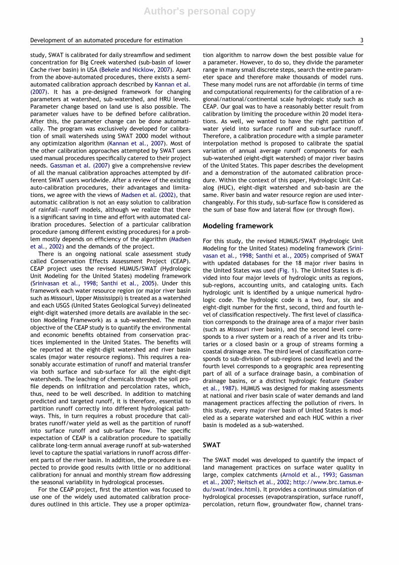
For this study, the revised HUMUS/SWAT (Hydrologic UnitModeling for the United States) modeling framework (Srini-vasan et al., 1998; Santhi et al., 2005) comprised of SWATwith updated databases for the 18 major river basins inthe United States was used (Fig. 1). The United States is di-vided into four major levels of hydrologic units as regions,sub-regions, accounting units, and cataloging units. Eachhydrologic unit is identified by a unique numerical hydro-logic code. The hydrologic code is a two, four, six andeight-digit number for the first, second, third and fourth le-vel of classification respectively. The first level of classifica-tion corresponds to the drainage area of a major river basin(such as Missouri river basin), and the second level corre-sponds to a river system or a reach of a river and its tribu-taries or a closed basin or a group of streams forming acoastal drainage area. The third level of classification corre-sponds to sub-division of sub-regions (second level) and thefourth level corresponds to a geographic area representingpart of all of a surface drainage basin, a combination ofdrainage basins, or a distinct hydrologic feature (Seaberet al., 1987). HUMUS was designed for making assessmentsat national and river basin scale of water demands and landmanagement practices affecting the pollution of rivers. Inthis study, every major river basin of United States is mod-eled as a separate watershed and each HUC within a riverbasin is modeled as a sub-watershed.

SWAT

The SWAT model was developed to quantify the impact ofland management practices on surface water quality inlarge, complex catchments (Arnold et al., 1993; Gassmanet al., 2007; Neitsch et al., 2002; http://www.brc.tamus.e-du/swat/index.html). It provides a continuous simulation ofhydrological processes (evapotranspiration, surface runoff,percolation, return flow, groundwater flow, channel trans-

Development of an automated procedure for estimation 3


mission losses, pond and reservoir storage, channel routingand field drainage), crop growth and material transfers (soilerosion, nutrient and organic chemical transport and fate).The model can be run with a daily time step, although sub-daily data can also be used. It incorporates the combinedand interacting effects of weather and land management(e.g. irrigation, planting and harvesting operations and theapplication of fertilizers, pesticides or other inputs). SWATdivides the watershed into sub-watersheds using topogra-phy. Each sub-watershed is divided into hydrological re-sponse units (HRUs), which are unique combinations of soiland land cover. Although individual HRU’s are simulatedindependently from one another, predicted water andmaterial flows are routed within the channel network,which allows for large catchments with hundreds or eventhousands of HRUs to be simulated.

Databases

The HUMUS/SWAT system requires several databases suchas land use, soils, management practices and weather. Forthe present study, recently available data are processedto update the HUMUS/SWAT databases and prepare theSWAT input files for the river basins (Santhi et al., 2005).

Land use

The United States Geological Survey (USGS)–National LandCover Data (NLCD) of 1992 is the spatial data currentlyavailable for land use at 30 m resolution for the UnitedStates (Vogelmann et al., 2001). For this study, the 1992USGS–NLCD land cover data set is used as the base, whichincludes agriculture, urban, pasture, range, forest, wet-land, barren and water.

Soils

Each land use within an eight-digit watershed is associatedwith soil data. Soil data required for SWAT were processed

from the STATe Soil GeOgraphic (STATSGO) database(USDA–NRCS, 1994). Each STATSGO polygon contains multi-ple soil series and the areal percentage of each soil series.Within a STATSGO polygon, the soil series with the largestarea was identified and the associated physical propertiesof the soil series were extracted for SWAT. This procedurewas followed for all the eight-digit watersheds (Santhiet al., 2005).

Topography

Topographic information on accumulated drainage area,overland field slope, overland field length, channel dimen-sions and channel slope were derived from the DEM dataof the previous HUMUS project (Srinivasan et al., 1998).

Management data

Management operations such as planting, harvesting, appli-cations of fertilizers, manure and pesticides and irrigationwater and tillage operations along with timings or potentialheat units are specified for various land uses in the manage-ment files. Management operations/inputs vary across re-gions. These data are gathered from various sources suchas Agricultural Census Data and USDA–National AgriculturalStatistics Service (NASS)’s agricultural chemical use data(Santhi et al., 2005).

Weather

Measured daily precipitation and maximum and minimumtemperature data sets from 1960 to 2001 are used in thisstudy. The precipitation and temperature data sets are cre-ated from a combination of point measurements of dailyprecipitation and temperature (maximum and minimum)(Eischeid et al., 2000) and Parameter-elevation Regressionson Independent Slopes Model (PRISM) (Daly et al., 1994,2002). The point measurements compose a serially com-plete (without missing values) data set processed from the

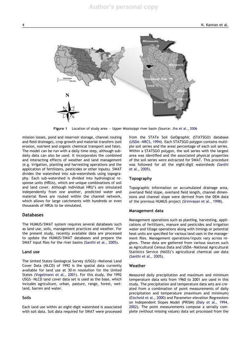
Figure 1 Location of study area – Upper Mississippi river basin (Source: Jha et al., 2006

4 N. Kannan et al.


National Climatic Data Center (NCDC) station records. PRISMis an analytical model that uses point data and a digital ele-vation model (DEM) to generate gridded estimates ofmonthly climatic parameters. PRISM data are distributedat a resolution of approximately 4 km2. A novel approachhas been developed to combine the point measurementsand the monthly PRISM grids to develop the distribution ofthe daily records with orographic adjustments over eachUSGS eight-digit watersheds (Di Luzio et al., 2008). Otherdata such as solar radiation, wind speed and relative humid-ity are simulated using the weather generator (Nicks, 1974;Sharpley and Williams, 1990) available within SWAT.

Target values for calibration

Sources of information

The target values for calibration are based on runoff con-tours for the entire United States prepared by Gebertet al. (1987). The preferred source of information for therunoff contours was stream flow recorded from 5951 UnitedStates Geological Survey (USGS) gauging stations during1951–1980 with no diversions and an area of not more thana HUC. If records for the 30-year period were not fully avail-able for a station, the records were extrapolated based on acorrelation (method suggested by Matalas and Jacobs, 1964)with a nearby station. If data from stations without diver-sions were not available, then data from stations with diver-sions were used with correction for diversions. If thegauging station records indicated an amount for the diver-sions, it was used to adjust the flow otherwise the diversionswere estimated based on other existing information. Irriga-tion diversions, commonly represented by number of acresirrigated were multiplied by the typical amount of waterused for irrigation in that area less an allowance for returnflows. These estimates of diversion were used to correct the

measured stream flow, which in turn was used for comput-ing runoff. If no information were available, estimates ofrunoff in adjacent areas, known variations of precipitationand elevation were used to compute runoff (Krug et al.,1989; Gebert et al., 1987). The data obtained as describedabove were used to produce runoff contours (lines joiningequal runoff values) for the entire United States. More de-tails on the procedure used for the preparation of runoffcontours are available in Krug et al. (1989) and Gebertet al. (1987).

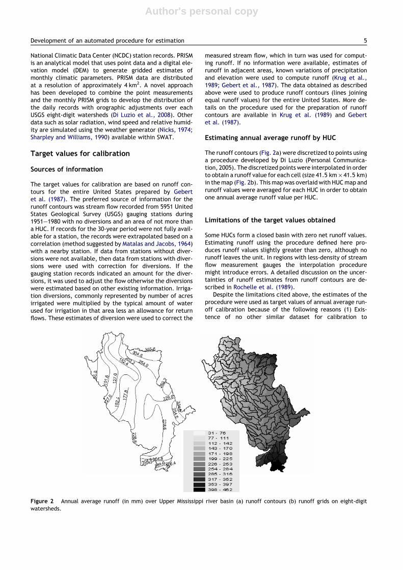
Estimating annual average runoff by HUC

The runoff contours (Fig. 2a) were discretized to points usinga procedure developed by Di Luzio (Personal Communica-tion, 2005). The discretized points were interpolated in orderto obtain a runoff value for each cell (size 41.5 km · 41.5 km)in themap (Fig. 2b). This mapwas overlaid with HUCmap andrunoff values were averaged for each HUC in order to obtainone annual average runoff value per HUC.

Limitations of the target values obtained

Some HUCs form a closed basin with zero net runoff values.Estimating runoff using the procedure defined here pro-duces runoff values slightly greater than zero, although norunoff leaves the unit. In regions with less-density of streamflow measurement gauges the interpolation proceduremight introduce errors. A detailed discussion on the uncer-tainties of runoff estimates from runoff contours are de-scribed in Rochelle et al. (1989).

Despite the limitations cited above, the estimates of theprocedure were used as target values of annual average run-off calibration because of the following reasons (1) Exis-tence of no other similar dataset for calibration to

Figure 2 Annual average runoff (in mm) over Upper Mississippi river basin (a) runoff contours (b) runoff grids on eight-digitwatersheds.



capture the spatial variation of runoff over region(s) orlarge river basins (2) Adequacy for the project (3) proce-dural simplicity and mathematical convenience.

A procedure similar to the above described is adopted forbase flow (briefly described here). Base flow availability var-ies over space and time in a region due to climate, topogra-phy, landscape, and geological characteristics. Santhi et al.(2008a) have estimated the base flow index (BFI) or baseflow ratio (ratio of base flow/total stream flow) from dailystreamflow records of the USGS stream gages using a recur-sive digital filter method developed by Arnold et al. (1995).Nearly 8600 USGS stream gage locations distributed acrossthe Conterminous United States were selected to estimatethe base flow index. Gages were selected with drainageareas of 50–1000 km2 to minimize the effects of flow rout-ing, and limit the influence of reservoir releases. Each se-lected gage had a minimum of 10 years of dailystreamflow observations. These base flow index values wereused to develop a smooth grid map of the base flow indexvalues using inverse distance weighting spatial interpolationmethod. To estimate the base flow, the base flow ratio mapwas multiplied by observed runoff map prepared by Gebertet al. (1987). The difference between runoff and sub-sur-face flow (or base flow) is assumed as surface runoff. Thedata obtained in this manner were used as targeted valuesfor calibration of runoff, sub-surface flow and surfacerunoff.

Methods

This section describes the development of an automatedprocedure for calibration of spatial variation of annual aver-age surface runoff, sub-surface flow and water yield overlarge river basins. In addition, the calibration procedure isexpected to provide satisfactory results (with little or noadditional calibration) for the predicted monthly meanstream flow when compared to observed time series atthe flow gauging stations. Data from 1960 is used as awarm-up period for the model to make the state variablesassume realistic initial values. Data from 1961–1990 is usedfor calibration and the remaining data from 1991–2001 isused for validation. Modeling was carried out at annual timestep using Hargreaves method (Hargreaves and Samani,1985) for estimation of ET and curve number method forrainfall–runoff modeling.

Introduction to model parameters

SWAT model has many parameters. Only the most sensitive(suggested in the user manual and other studies) nineparameters are used for the calibration procedure. Theyare (1) harg_petco (a coefficient used to adjust evapotrans-piration (ET) estimated by Hargreaves method (Hargreavesand Samani, 1985) and water yield; (2) soil water depletioncoefficient (a coefficient used to adjust surface runoff andsub-surface flow in accordance with soil water depletion)(Kannan et al., 2008); (3) curve number (CN) to adjust sur-face runoff; (4) groundwater re-evaporation coefficient(GWREVAP). It controls the upward movement of waterfrom shallow aquifer to root zone in proportion to evapora-tive demand; (5) minimum depth of water in soil for base

flow to occur (GWQMN). Groundwater flow is allowed onlyif the depth of water in the shallow aquifer is equal to orgreater than the GWQMN parameter value; (6) soil availablewater holding capacity (AWC); (7) slope length (used to con-trol lateral flow estimates-particularly from high-slopeareas); (8) plant evaporation compensation coefficient(EPCO). This controls the depth distribution of water in soillayers to meet plant evaporative demand and (9) soil evap-oration compensation coefficient (ESCO), which controls thedepth distribution of water in soil layers to meet soil evap-orative demand. Among the nine parameters harg_petco,depletion coefficient, GWREVAP, GWQMN are sub-basin le-vel parameters and the other parameters operate at Hydro-logic Response Unit (HRU) [sub-division of a sub-basin] level(Neitsch et al., 2002).

Development of the calibration procedure

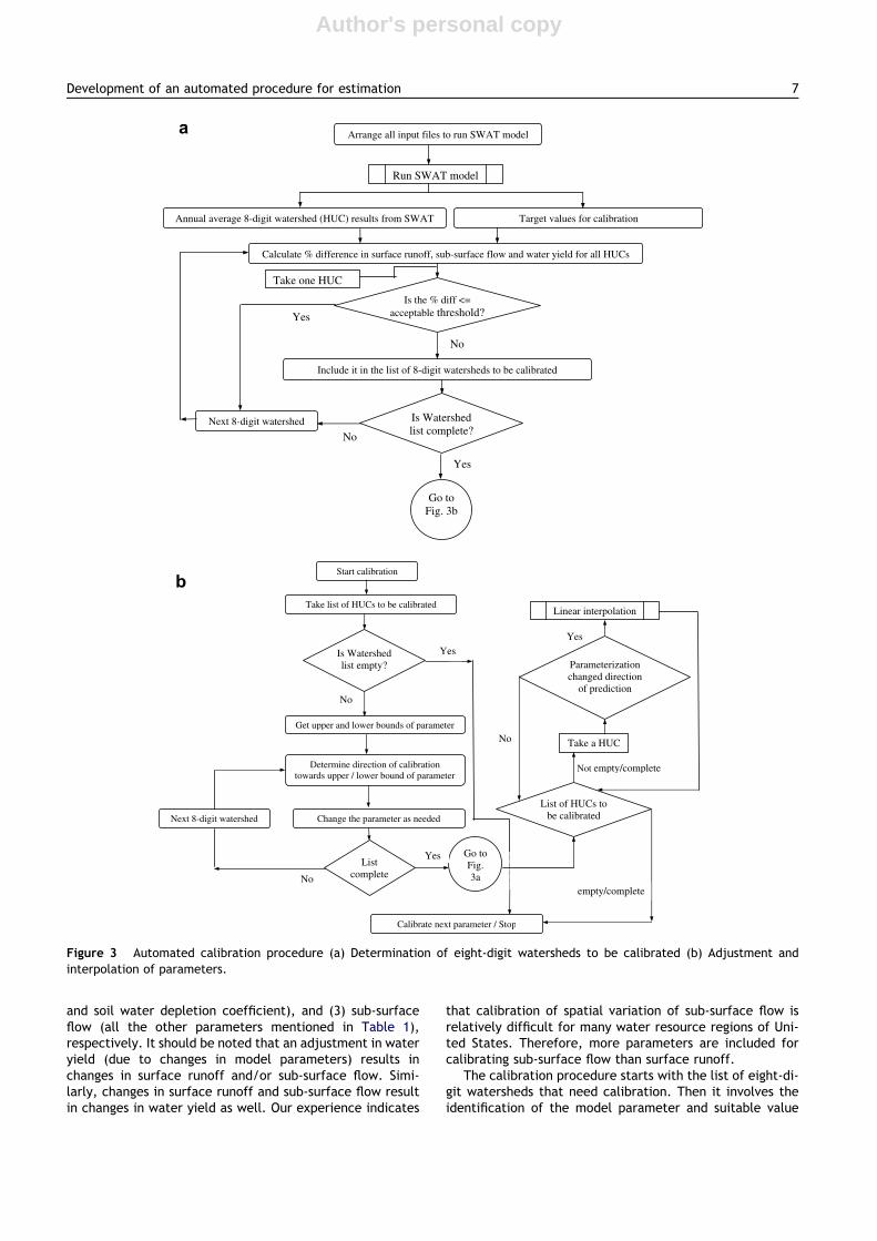
The calibration procedure discussed here is somewhat dif-ferent from other existing automated calibration proce-dures. The differences are (i) It is developed forcalibration of spatial variation of runoff over large river ba-sins, (ii) It calibrates different components of runoff such assurface runoff, sub-surface flow apart from water yield, (iii)Objective of calibration is different at different stages ofthe calibration procedure (obtaining close match betweenpredicted and targeted values of water yield, surface runoffand sub-surface flow at steps 1–3, respectively), and (iv)the termination criterion is the percentage difference be-tween prediction and targeted value (this is 20 %, 10 %,and 10 % for water yield, surface runoff and sub-surfaceflow, respectively). The development of the automated cal-ibration procedure is discussed in two sections viz. (a) Sep-aration of eight-digit watersheds (within a water resourceregion) that require calibration and (b) calibrationprocedure.

Separation of eight-digit watersheds requiring calibrationThe preliminary requirements for using the calibration pro-cedure are the arrangement of the necessary input files forrunning SWAT model for a particular river basin and obtain-ing the target values of annual average estimates of surfacerunoff, sub-surface flow and water yield for each eight-digitwatershed in that river basin. As well, it requires a list ofmodel parameters to be used in calibration along with theirranges as input. After having the two above-mentionedrequirements, the next step involves running the SWATmodel without any calibration. Then the procedure involvesestimation of the percentage difference between annualaverage predictions and target values of surface runoff,sub-surface flow and water yield for each eight-digit wa-tershed in the river basin. Based on the estimated percent-age difference on the stipulated criteria (10%, 10% and 20%differences between predictions and target values), theeight-digit watersheds requiring calibration are identifiedand stored in a separate file (Fig. 3a).

Calibration procedureThe calibration process is carried out in three major stepsviz. (1) calibration of water yield (parameterization ofharg_petco), (2) surface runoff (parameterization of CN

6 N. Kannan et al.


and soil water depletion coefficient), and (3) sub-surfaceflow (all the other parameters mentioned in Table 1),respectively. It should be noted that an adjustment in wateryield (due to changes in model parameters) results inchanges in surface runoff and/or sub-surface flow. Simi-larly, changes in surface runoff and sub-surface flow resultin changes in water yield as well. Our experience indicates

that calibration of spatial variation of sub-surface flow isrelatively difficult for many water resource regions of Uni-ted States. Therefore, more parameters are included forcalibrating sub-surface flow than surface runoff.

The calibration procedure starts with the list of eight-di-git watersheds that need calibration. Then it involves theidentification of the model parameter and suitable value

Arrange all input files to run SWAT model

ut files to run SWAT model

Run SWAT model

Annual average 8-digit watershed (HUC) results from SWAT Target values for calibration

Calculate % difference in surface runoff, sub-surface flow and water yield for all HUCs

Include it in the list of 8-digit watersheds to be calibrated

Is Watershed list complete?

Next 8-digit watershed

Is the % diff <= acceptable threshold?Yes

No

No

Yes

Take one HUC

Go to Fig. 3b

a

Is Watershed list empty?

Next 8-digit watershed

Start calibration

Get upper and lower bounds of parameter

Determine direction of calibrationtowards upper / lower bound of parameter

Change the parameter as needed

Linear interpolation

Listcomplete

Yes

No

Yes

No

Not empty/complete

No

Take list of HUCs to be calibrated

List of HUCs to be calibrated

Go to Fig.3a

Parameterizationchanged direction

of prediction

Take a HUC

Calibrate next parameter / Stop

empty/complete

Yes

b

Figure 3 Automated calibration procedure (a) Determination of eight-digit watersheds to be calibrated (b) Adjustment andinterpolation of parameters.



for that parameter (Table 1), which is based on the percent-age difference between predictions and target values. A po-sitive difference indicates over-estimation and vice versa.Based on under/over-estimation, the new value of a param-eter is selected as the upper/lower value (from the rangeassumed (see Table 1)). The next step is replacing the oldparameter value with the new value. The above-processesare repeated for all the eight-digit watersheds that needcalibration (result of section 1 of calibration procedure).Another SWAT run is made with the modified set of inputparameters. Then section 1 of calibration procedure(Fig. 3a) is repeated to identify the eight-digit watershedsstill requiring calibration.

Each eight-digit watershed needing calibration in theprevious step is analyzed to check whether the parameterchange (at the present step) has improved the estimation.If the estimation has improved and further calibration isnot needed (% difference between predictions and targetvalues of surface runoff, sub-surface flow and water yieldare within or equal to the stipulated criteria), that particu-lar eight-digit watershed is eliminated from the calibrationprocedure. If the estimation has improved and further cali-bration is needed and the direction of estimation has notchanged (e.g. under-estimation of surface runoff beforeand after parameter change), the procedure proceeds tonext parameter. If the estimation has improved and furthercalibration is needed and if the direction of estimation haschanged (e.g. under-estimation before parameter changeand over-estimation after parameter change), a new valuefor the same parameter is estimated based on a linear inter-polation technique using the parameter values at the previ-ous and present step and the percentage differences atprevious and present step (Fig. 3b). The linear interpolationmethod is used in the calibration procedure for finding abetter value for a particular parameter. It should be notedthat linear interpolation may not work well for some param-eters (e.g. GWQMN) that show very high sensitivity to sur-face or sub-surface flow within a short-range. However,linear interpolation is still used in the calibration procedureowing to its simplicity, convenience, unimodal nature of re-sponse for parameterization (a progressive increase/de-crease in parameter will cause a progressive increase/decrease in model output, and the direction of response will

not change) and the ability to find a better value. In the sec-ond iteration, the above procedure is repeated for all theHUCs that need estimation of a new value of parameterbased on linear interpolation (Fig. 3b). The calibration pro-cedure is carried out (in a similar fashion described in theprevious sections ‘Separation of eight-digit watershedsrequiring calibration’ and ‘Calibration procedure’) for allthe other parameters included in the procedure, one byone. The parameterization proceeds in the following order:harg_petco, depletion coefficient, CN, GWREVAP, GWQMN,AWC, Slope length, EPCO and ESCO. The entire automatedcalibration procedure is written in FORTRAN.

Results

Effects of initial parameter values on calibration

Unless altered by the user, the calibration procedure usesdefault initial parameters written by the user interface.The parameter CN is a unique value obtained from a lookup table (within the interface) for a particular combinationof soil and land use. Therefore, the initial value for thisparameter is also fixed. Available Water Capacity (AWC),the property of a particular soil layer is obtained from thesoil database. Therefore, the initial value of AWC is alsofixed. Slope length for a particular HRU is obtained fromthe DEM and hence the user for the initial condition maynot alter its value. However, the other model parameters(harg_petco, depletion coefficient, GWREVAP, GWQMN,EPCO, and ESCO) can have any initial value within the al-lowed range. Therefore, an analysis is done to ascertainwhether there are differences in results by having initial val-ues other than the default. The initial value of only onemodel parameter is changed at a time; all the other param-eters are kept at their default initial values (Table 2a). Forthis analysis, the lower and upper limits of a parameter arechosen, and the calibration procedure is used in each trialindependently (starting from a no calibration scenario).Only one experiment was possible for the parameterGWQMN. This is because the default initial value of thisparameter was 0.0 (range of adjustment ± 3) for the HUC7020008 and the parameter cannot take negative values.

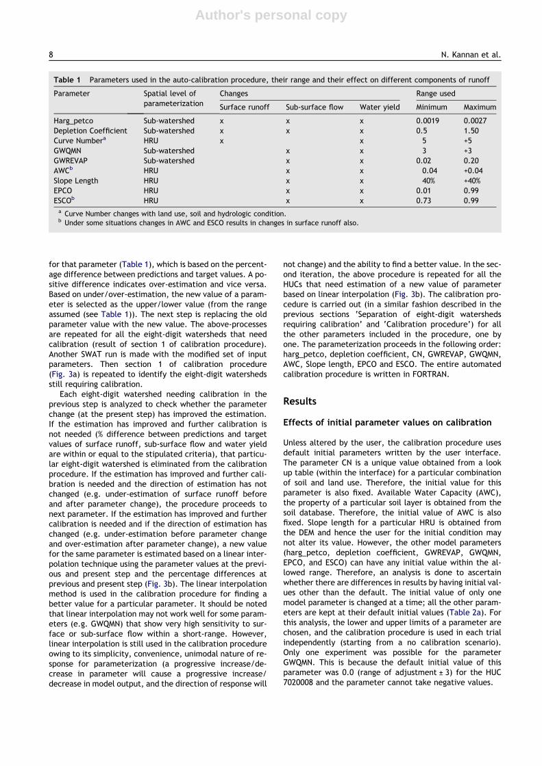
Table 1 Parameters used in the auto-calibration procedure, their range and their effect on different components of runoff

Parameter Spatial level ofparameterization

Changes Range used

Surface runoff Sub-surface flow Water yield Minimum Maximum

Harg_petco Sub-watershed x x x 0.0019 0.0027Depletion Coefficient Sub-watershed x x x 0.5 1.50Curve Numbera HRU x x �5 +5GWQMN Sub-watershed x x �3 +3GWREVAP Sub-watershed x x 0.02 0.20AWCb HRU x x �0.04 +0.04Slope Length HRU x x �40% +40%EPCO HRU x x 0.01 0.99ESCOb HRU x x 0.73 0.99a Curve Number changes with land use, soil and hydrologic condition.b Under some situations changes in AWC and ESCO results in changes in surface runoff also.

8 N. Kannan et al.


The predicted results of surface runoff, sub-surface flowand water yield for different initial values of parameters areshown in Table 2a. Considering the stipulated criteria forcalibration (10%, 10%, and 20% differences between predic-tions and target values), the results from the experimentsusing different initial parameters are very similar to the re-sults of default initial parameters although there existssome marginal numerical differences. On an average, thedifferences exhibited by the different initial parametercombination to that of default initial values are 0.9 mm,2.8 mm and 3.7 mm, respectively, for surface runoff, sub-surface flow, and water yield. The maximum differences ob-served are 3.5 mm in surface runoff, 7.8 mm in sub-surfaceflow and 10.7 mm in water yield. Experiments with initialEPCO value of 0.99 and initial ESCO value of 0.73 bringslightly different results than that of default initial values.All the other experiments bring very similar results. Thisshows that the calibration procedure brings similar resultsirrespective of the initial parameter values.

Demonstration of auto-calibration procedure

A demonstration of the auto-calibration procedure is givenin Table 2b using the eight-digit watershed 07020008 ofthe Upper Mississippi river basin (shaded area in black nearthe left river basin boundary in Fig. 1). From Table 2b it canbe seen that the percentage difference between predictedand targeted water yield at the beginning is within the stip-ulated value (4.2% existing vs. 20% target). Therefore,harg_petco was not parameterized to adjust the water yield(Table 2b). However, the percentage difference betweenpredicted and targeted annual average surface runoff is be-yond the threshold (�54% existing vs. 10% threshold) indi-cating under-estimation of surface runoff. Therefore,depletion coefficient is adjusted to bring predicted surfacerunoff within 10% of targeted value. In doing so, the under-estimation (before depletion coefficient parameterization)

has changed to over-estimation after depletion coefficientparameterization. Hence, a linear interpolation was per-formed to identify the suitable value for depletion coeffi-cient that keeps the predicted surface runoff within 10%of targeted value. After the adjustment of depletion coeffi-cient, the percentage difference between predictions andtarget values of annual average surface runoff is 1.9% (with-in the target) eliminating the need for further adjustment ofsurface runoff using CN (Table 2b). Although the predictedwater yield is still within 20% of target value (after adjust-ment of depletion coefficient), the sub-surface flow is notwithin the target value of 10%. Therefore, sub-surface flowwas adjusted using the suitable parameters (Table 2b).After the parameterization of GWREVAP, GWQMN, slopelength, EPCO, and ESCO, respectively, the predicted annualaverage sub-surface flow for the HUC 07020008 is broughtwithin 10% (Table 2b). In Table 2b, the predicted values ofsurface runoff, sub-surface flow and water yield and thepercentage difference between predictions and target val-ues are shown at every step of calibration for better under-standing of the calibration procedure.

Demonstration of parameterization

In the previous section, a demonstration of the entire pro-cedure used for calibration is discussed. In this section, adetailed discussion of calibration of one parameter is pre-sented to show how the parameterization is carried out.Parameterization of the depletion coefficient is used forthis demonstration.

Nature of the depletion coefficient parameterAn increase in depletion coefficient causes an increase insurface runoff and a decrease in sub-surface flow withoutappreciably affecting the water yield (Kannan et al.,2008). Although a change in depletion coefficient affectsboth surface runoff and sub-surface flow, in this calibration

Table 2a Effects of initial parameter values on calibration: demonstration of results using an eight-digit watershed (7020008)from Upper Mississippi river basin

Parameter Initial Values Predicted values after calibration (mm)

Surface runoff Sub-Surface flow Water Yield

All parameters Defaulta 45.1 37.14 82.24Harg_petco 0.0019 46.12 39.49 85.61Harg_petco 0.0027 46.12 39.49 85.61Depletion coefficient 0.5 46.12 39.49 85.61Depletion coefficient 1.5 46.12 39.49 85.61GWREVAP 0.02 46.12 42.17 88.29GWREVAP 0.2 46.12 39.25 85.36GWQMN 3 47.46 34.9 82.36EPCO 0.01 44.03 42.15 86.17EPCO 0.99 41.6 34.95 76.54ESCO 0.73 48.05 44.92 92.97ESCO 0.99 48.31 42.79 91.1

Target values Not applicable 44.3 40.1 84.4a The initial parameter values were 0.0023, 0.75, 0.10, 0.0, 0.0, and 0.95 for harg_petco, depletion coefficient, GWREVAP, GWQMN,

EPCO, and ESCO, respectively.



procedure, the depletion coefficient is adjusted to obtain agood match between predictions and target values of sur-face runoff rather than sub-surface flow because the sub-surface flow calibration is performed after the surface run-off calibration using the depletion coefficient (Table 1).

Parameterization of depletion coefficientWith the initial value of depletion coefficient (0.75) (andwithout any adjustment of the other parameters used inthe calibration procedure), surface runoff is under-esti-mated and sub-surface flow is over-estimated (row 1 ofTable 3) with respect to the target values. Therefore, toaddress under-estimation of surface runoff and over-esti-mation of sub-surface flow, the depletion coefficient is in-creased from 0.75 (initial value) to 1.5 (the upper limitassumed for calibration). This results in over-estimationof surface runoff. On the other hand, the severe over-esti-mation of sub-surface flow at the beginning is controlledbecause of the change in depletion coefficient (row 2 ofTable 3). This shows that a depletion coefficient valueof 0.75 is too low and 1.5 is too high to get a reasonable

match of predicted and targeted surface runoff. There-fore, an interpolation of depletion coefficient is carriedout between 0.75 and 1.5 based on the percentage differ-ence between predicted and targeted value of surfacerunoff at the previous (row 1 of Table 3) and present cal-ibration steps (row 2 of Table 3). Using the interpolatedvalue of 1.32 for depletion coefficient, the predicted sur-face runoff (45.13 mm) is close to the target value(44.3 mm).

Evaluation of the performance of the automatedcalibration procedure

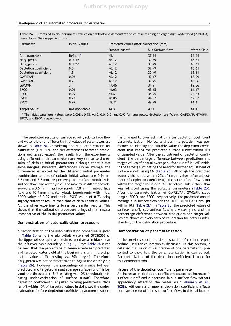
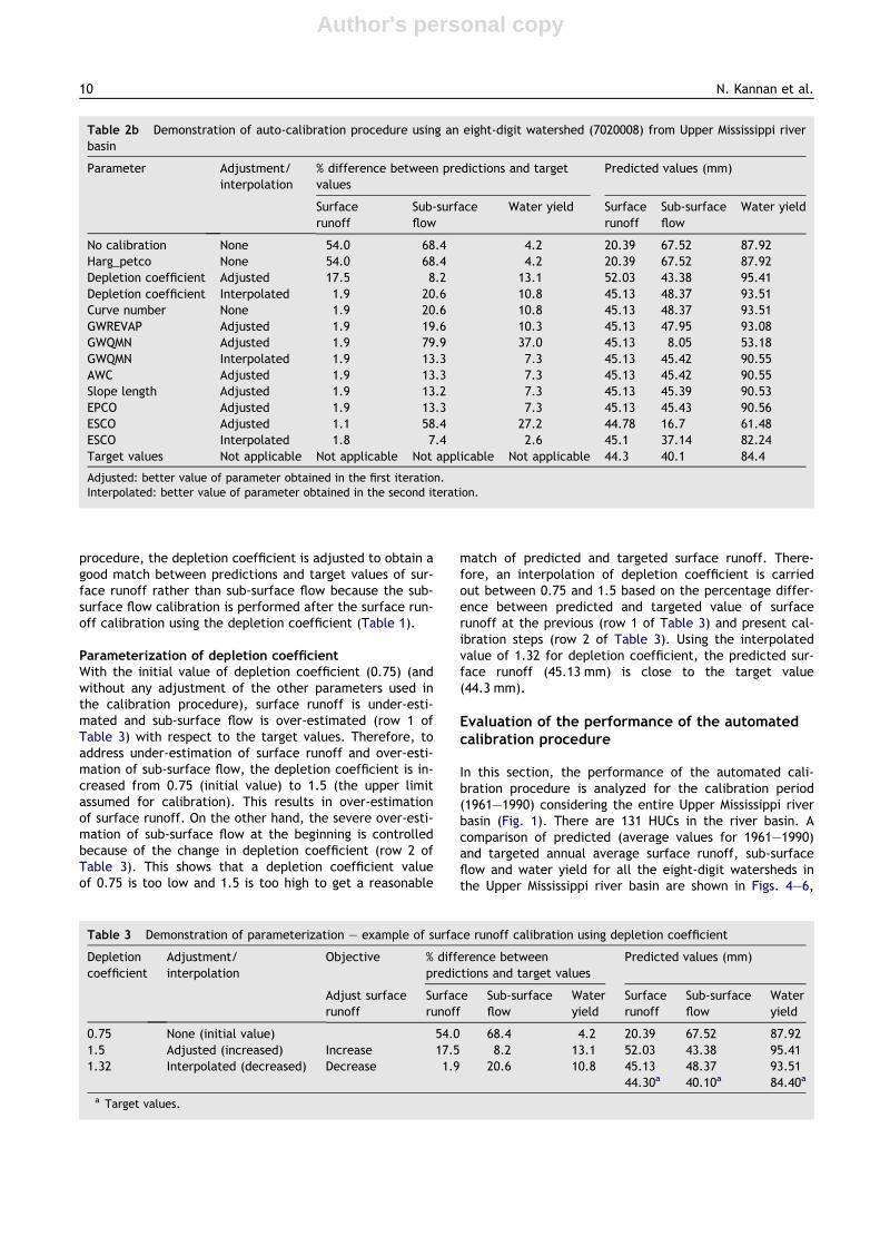
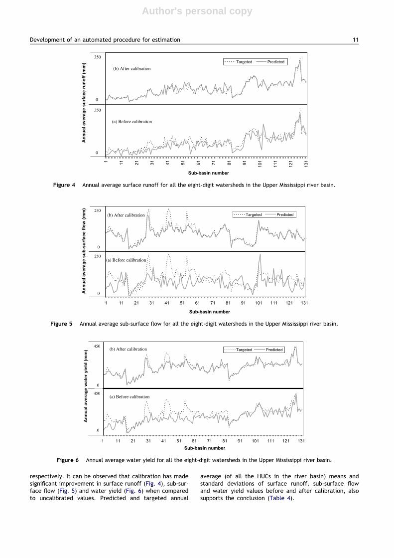
In this section, the performance of the automated cali-bration procedure is analyzed for the calibration period(1961–1990) considering the entire Upper Mississippi riverbasin (Fig. 1). There are 131 HUCs in the river basin. Acomparison of predicted (average values for 1961–1990)and targeted annual average surface runoff, sub-surfaceflow and water yield for all the eight-digit watersheds inthe Upper Mississippi river basin are shown in Figs. 4–6,

Table 2b Demonstration of auto-calibration procedure using an eight-digit watershed (7020008) from Upper Mississippi riverbasin

Parameter Adjustment/interpolation

% difference between predictions and targetvalues

Predicted values (mm)

Surfacerunoff

Sub-surfaceflow

Water yield Surfacerunoff

Sub-surfaceflow

Water yield

No calibration None �54.0 68.4 4.2 20.39 67.52 87.92Harg_petco None �54.0 68.4 4.2 20.39 67.52 87.92Depletion coefficient Adjusted 17.5 8.2 13.1 52.03 43.38 95.41Depletion coefficient Interpolated 1.9 20.6 10.8 45.13 48.37 93.51Curve number None 1.9 20.6 10.8 45.13 48.37 93.51GWREVAP Adjusted 1.9 19.6 10.3 45.13 47.95 93.08GWQMN Adjusted 1.9 �79.9 �37.0 45.13 8.05 53.18GWQMN Interpolated 1.9 13.3 7.3 45.13 45.42 90.55AWC Adjusted 1.9 13.3 7.3 45.13 45.42 90.55Slope length Adjusted 1.9 13.2 7.3 45.13 45.39 90.53EPCO Adjusted 1.9 13.3 7.3 45.13 45.43 90.56ESCO Adjusted 1.1 �58.4 �27.2 44.78 16.7 61.48ESCO Interpolated 1.8 �7.4 �2.6 45.1 37.14 82.24Target values Not applicable Not applicable Not applicable Not applicable 44.3 40.1 84.4

Adjusted: better value of parameter obtained in the first iteration.Interpolated: better value of parameter obtained in the second iteration.

Table 3 Demonstration of parameterization – example of surface runoff calibration using depletion coefficient

Depletioncoefficient

Adjustment/interpolation

Objective % difference betweenpredictions and target values

Predicted values (mm)

Adjust surfacerunoff

Surfacerunoff

Sub-surfaceflow

Wateryield

Surfacerunoff

Sub-surfaceflow

Wateryield

0.75 None (initial value) �54.0 68.4 4.2 20.39 67.52 87.921.5 Adjusted (increased) Increase 17.5 8.2 13.1 52.03 43.38 95.411.32 Interpolated (decreased) Decrease 1.9 20.6 10.8 45.13 48.37 93.51

44.30a 40.10a 84.40a

a Target values.

10 N. Kannan et al.


respectively. It can be observed that calibration has madesignificant improvement in surface runoff (Fig. 4), sub-sur-face flow (Fig. 5) and water yield (Fig. 6) when comparedto uncalibrated values. Predicted and targeted annual

average (of all the HUCs in the river basin) means andstandard deviations of surface runoff, sub-surface flowand water yield values before and after calibration, alsosupports the conclusion (Table 4).

1 11 21 31 41 51 61 71 81 91 101

111

121

131

Sub-basin number

Ann

ual a

vera

ge s

urfa

ce ru

noff

(mm

) Targeted Predicted

0

350

0

350

(a) Before calibration

(b) After calibration

Figure 4 Annual average surface runoff for all the eight-digit watersheds in the Upper Mississippi river basin.

1 11 21 31 41 51 61 71 81 91 101 111 121 131

Sub-basin number

Ann

ual a

vera

ge s

ub-s

urfa

ce fl

ow (m

m)

0

250

0

250(b) After calibration


Targeted Predicted

Figure 5 Annual average sub-surface flow for all the eight-digit watersheds in the Upper Mississippi river basin.

1 11 21 31 41 51 61 71 81 91 101 111 121 131Sub-basin number

Ann

ual a

vera

ge w

ater

yie

ld (m

m) Targeted Predicted

0

450

450

0


(b) After calibration

Figure 6 Annual average water yield for all the eight-digit watersheds in the Upper Mississippi river basin.



Performance evaluation of model before and after cali-bration using Nash and Sutcliffe prediction efficiency andR2 are given in Table 5. From Table 5, it can be seen thatthe prediction efficiency has improved significantly aftercalibration (in particular for sub-surface flow and wateryield) when compared to prediction efficiency before cali-bration. In addition, the number of HUCs requiring calibra-tion (out of 131 HUCs in the Upper Mississippi river basin)has decreased appreciably after calibration (Fig. 7,Table 5).

Analysis of eight-digit watersheds with inadequatecalibration

The automated calibration procedure developed in thisstudy, carried out surface runoff calibration satisfactorily(Fig. 4). However, a visual inspection of the predicted andtargeted values of water yield (Fig. 6) reveals that a fewHUCs were not adequately calibrated. For detailed exami-nation, three HUCs 7050001, 7050002, and 7050003 (Sub wa-tershed numbers 41–43) were chosen. These HUCs show the

Table 4 Comparison of basin-average predicted and target runoff components

Model performance evaluation criteria Surface runoff Sub-surface flow Water yield

Before calibration Mean (mm) 87.8 81.3 169.1Standard deviation (mm) 55.3 34.8 61.5

After calibration Mean (mm) 106.3 94.5 200.8Standard deviation (mm) 50.7 35.0 64.9

Target values Mean (mm) 101.9 101.2 203.1Standard deviation (mm) 49.7 41.7 66.4

Table 5 Model performance evaluation criteria for the river basin

Calibration Model performance evaluation criteria Surface runoff Sub-surface flow Water yield

Before calibration Nash and Sutcliffe efficiency (%) 65.8 �47.5 21.2R2 0.67 �0.43 0.38Eight-digit watersheds needing calibration 97 112 52

After calibration Nash and Sutcliffe efficiency (%) 93.9 83 93.3R2 0.95 0.86 0.93Eight-digit watersheds needing calibration 18 26 5

Figure 7 Percentage difference between predictions and target values after calibration (hatched areas are not within targetvalues).

12 N. Kannan et al.


maximum difference between predicted and targeted wateryield. The differences are mainly due to the under-estima-tion of sub-surface flow (Fig. 5) which in turn is due toover-estimation of ET by Hargreaves method in forest andforested wetlands which account for 55–65 % of the areaof the sub-watersheds analysed. Changing harg_petcoparameter to the lower bound (using the calibration proce-dure) in order to reduce ET values was not adequate forthese HUCs, although this is not the case for other HUCscalibrated.

Application of the calibration procedure

In connection with the CEAP study, the calibration proce-dure described in this article is used for calibration of Ohioriver basin and Arkansas–White–Red river basins coveringtwo different hydrological conditions (high flow and lowflow) (Santhi et al., 2008b). Spatial variation of runoffacross the two river basins was calibrated using the auto-mated procedure and satisfactory results were obtained(R2 values of 0.78 and 0.99 were obtained between pre-dicted and targeted annual average runoff for Ohio andArkansas–White–Red river basins, respectively). When val-idated at gauging stations, for annual and monthly streamflow, good results were obtained for both the river basins.For the Ohio basin, 86% and 72% Nash and Sutcliffe effi-ciency values were obtained at the annual and monthly timesteps. For the same region, R2 values (predictions vs. obser-vations) of 0.94 and 0.83 were obtained at the annual andmonthly time steps. For the Arkansas–White–Red river ba-sins basin, 79% and 64% Nash and Sutcliffe efficiency valueswere obtained for annual and monthly stream flow. For thesame region, R2 values (predictions vs. observations) of 0.86and 0.66 were obtained for annual and monthly stream flow.More details on the study area, range of values for differentparameters and results can be found in Santhi et al. (2008b).The study by Santhi et al. (2008b), has shown that the cali-bration procedure outlined in this article is capable of cali-brating river basins with a range of hydrological conditions.

Limitations of the procedure

Unlike the standard automated calibration procedures, theprocedure described here does not cover all the possiblecombinations of parameters. It does not use multiple objec-tives for carrying out calibration. It uses a simple linearinterpolation technique for finding a better value of aparameter instead of search procedure as used in the otherauto-calibration procedures. Some fine-tuning of modelparameters may be required for HUCs with inadequatecalibration.

Summary and conclusions

United States Department of Agriculture has implementedmany conservation practices throughout the country to re-duce the pollution of soil and water. A national assessmentstudy called ‘‘Conservation Effects Assessment Project’’ isongoing with the objective of quantifying the environmentaland economic benefits obtained from those conservationpractices. The study considers major water resource regions

(or river basins) as watershed boundaries and hydrologicmodelling of the river basins with reasonable accuracy is apre-requisite to achieve the objectives of the project. Forhydrologic modelling of the entire United States with rea-sonable accuracy, a simple, methodical automated proce-dure is developed to calibrate the spatial variation ofrunoff and the partitioning of runoff into surface runoffand sub-surface flow for each eight-digit watershed. Thedeveloped calibration procedure is described and demon-strated with example results from Upper Mississippi river ba-sin. Based on the results obtained from the study thefollowing conclusions can be drawn.

1. A simple methodical automated procedure is developedto calibrate the spatial variation of annual average run-off components for large-scale hydrologic modelingstudies.

2. The simple linear interpolation algorithm is performingsatisfactorily in identifying better parameter values formost of the parameters included in the calibrationprocedure.

3. Test results from Upper Mississippi river basin suggestthat the annual average surface runoff, sub-surface flowand water yield values are calibrated satisfactorily usingthe calibration procedure developed

4. Selection of the suitable range of parameter values iscrucial for getting desired results from the calibrationprocedure.

5. Test results from the calibration procedure are promisingand show great potential for its use to all the 18 majorriver basins of the United States and similar large-scalestudies using SWAT.

References

Arnold, J.G., Allen, P.M., Bernhardt, G., 1993. A comprehensivesurface-groundwater flow model. Journal of Hydrology 142, 47–69.

Arnold, J.G., Allen, P.M., Muttiah, R., Bernhardt, G., 1995.Automated base flow separation and recession analysis tech-niques. Ground Water 33, 1010–1018.

Bekele, E.G., Nicklow, J.W., 2007. Multi-objective automaticcalibration of SWAT using NSGA-II. Journal of Hydrology 341,165–176.

Daly, C., Gibson, W.P., Taylor, G.H., Johnson, G.L., Pasteris, P.,2002. A knowledge-based approach to the statistical mapping ofclimate. Climate Research 22, 99–113.

Daly, C.R., Neilson, P., Phillips, D.L., 1994. A statistical-topo-graphic model for mapping climatological precipitation overmountainous terrain. Journal of Applied Meteorology 33, 140–158.

Deb, K., 2001. Multi-objective Optimization Using EvolutionaryAlgorithms. Wiley, Chichester, UK.

Di Luzio, M., Arnold, J.G., 2004. Formulation of a hybrid calibrationapproach for a physically based distributed model with NEXRADdata input. Journal of Hydrology 298 (1–4), 136–154.

Di Luzio, M., Johnson, G.L., Daly, C., Eischeid, J., Arnold, J.G.,2008. Constructing Retrospective gridded daily precipitation andtemperature datasets for the conterminous United States.Journal of Applied Meteorology and Climatology 47 (2), 475–497.

Doherty, J., 2005. PEST: Model Independent Parameter Estimation.Fifth Edition of User Manual. Watermark Numerical Computing,Brisbane.



Duan, Q., Sorooshian, S., Gupta, V.K., 1992. Effective and efficientglobal optimization for conceptual rainfall–runoff models.Water Resources Research 24 (7), 1163–1173.

Duan, Q., Gupta, V.K., Sorooshian, S., 1993. A shuffled complexevolution approach for effective and efficient optimization.Journal of Optimization Theory and Applications 76 (3), 501–521.

Duan, Q., Sorooshian, S., Gupta, V.K., 1994. Optimal use of the SCE-UA global optimization method for calibrating watershed mod-els. Journal of Hydrology 158, 265–284.

Eckhardt, K., Arnold, J.G., 2001. Automatic calibration of adistributed catchment model. Journal of Hydrology 251, 103–109.

Eckhardt, K., Fohrer, N., Frede, H.G., 2005. Automatic modelcalibration. Hydrological Processes 19 (3), 651–658.

Eischeid, J.K., Pasteris, P.A., Diaz, H.F., Plantico, M.S., Lott, N.J.,2000. Creating a serially complete, national daily time series oftemperature and precipitation for the Western United States.Journal of Applied Meteorology 39, 1580–1591.

Gan, T.Y., Biftu, G.F., 1996. Automatic calibration of conceptualrainfall–runoff models: Optimization algorithms, catchmentconditions, and model structure. Water Resources Research 32(12), 3513–3524.

Gassman, P.W., Reyes, M.R., Green, C.H., Arnold, J.G., 2007. Thesoil and water assessment tool: historical development, appli-cations and future research directions. Transactions of theAmerican Society of Agricultural and Biological Engineers 50 (4),1211–1250.

Gebert, W.A., Graczyk, D.J., Krug, W.R., 1987. Annual averagerunoff in the United States, 1951–1980: US Geological SurveyHydrologic Investigations Atlas HA-710, 1 sheet, scale1:7,500,000.

Gupta, H.V., Sorooshian, S., Yapo, P.O., 1998. Toward improvedcalibration of hydrologic models: Multiple and non-commensu-rable measures of information. Water Resources Research 34(4), 751–763.

Hargreaves, G.H., Samani, Z.A., 1985. Reference crop evapotrans-piration from temperature. Applied Engineering in Agriculture 1(2), 96–99.

Hogue, T.S., Sorooshian, S., Gupta, H., Holz, A., Braatz, D., 2000. Amultistep automatic calibration scheme for river forecastingmodels. Journal of Hydrometeorology 1, 524–542.

Immerzeel, W.W., Droogers, P., 2008. Calibration of a distributedhydrological model based on satellite evapotranspiration. Jour-nal of Hydrology 349 (3–4), 411–424.

Jha, M., Arnold, J.G., Gassman, P.W., Giorgi, F., Gu, R.R., 2006.Climate change sensitivity assessment on Upper Mississippi RiverBasin streamflows using SWAT. Journal of American WaterResources Association 42 (4), 997–1016.

Johnston, P.R., Pilgrim, D., 1976. Parameter optimization forwatershed models. Water Resources Research 12 (3),477–486.

Kannan, N., Santhi, C., Williams, J.R., Arnold, J.G., 2008. Devel-opment of a continuous soil moisture accounting procedure forcurve number methodology and its behaviour with differentevapotranspiration methods. Hydrological Processes 22 (13),2114–2121.

Kannan, N., White, S.M., Worrall, F., Whelan, M.J., 2007. Sensitiv-ity analysis and identification of the best evapotranspiration andrunoff options for hydrological modelling in SWAT-2000. Journalof Hydrology 332, 456–466.

Krug, W.R., Gebert, W.A., Graczyk, D.J., 1989. Preparation ofannual average runoff map of the United States, 1951–80. OpenFile Report No. 87-535.

Lenhart, T., Kckhardt, K., Fohrer, N., Frede, H.G., 2002. Compar-ison of two different approaches of sensitivity analysis. Physicsand Chemistry of Earth 27, 645–654.

Madsen, H., 2000. Automatic calibration of a conceptual rainfall–runoff model using multiple objectives. Journal of Hydrology235, 276–288.

Madsen, H., Wilson, G., Ammentorp, H.C., 2002. Comparison ofdifferent automated strategies for calibration of rainfall–runoffmodels. Journal of Hydrology 261, 48–59.

Matalas, N.C., Jacobs, B., 1964. A correlation procedure foraugmenting hydrologic data: United States Geological Surveyprofessional paper 434-E, 7pp.

Muleta, M.K., Nicklow, J.W., 2005. Sensitivity and uncertaintyanalysis coupled with automatic calibration for a distributedwatershed model. Journal of Hydrology 306, 127–145.

Neitsch, S.L., Arnold, J.G., Kiniry, J.R., Williams, J.R., King K.W.,2002. Soil and Water Assessment Tool Theoretical Documenta-tion: Version 2000. GSWRL Report 02-01, BRC Report 02-05,Publ. Texas Water Resources Institute, TR-191. College Station,TX, 458pp.

Nicks, A.D., 1974. Stochastic generation of the occurrence, patternand location of maximum amount of rainfall. In: Proc. Sympo-sium on Statistical Hydrology, Misc. Publ. No. 1275. Washington,DC, USDA, pp. 154–171.

Rochelle, B.P., Stevens, D.L., Church, R., 1989. Uncertaintyanalysis of runoff estimates from a runoff contour map. WaterResources Bulletin 25 (3), 491–498.

Santhi, C., Allen, P.M., Muttiah, R.S., Arnold, J.G., Tuppad, P.,2008a. Regional estimation of base flow for the conterminousUnited States by Hydrologic Landscape Regions. Journal ofHydrology 351 (1–2), 139–153.

Santhi, C., Kannan, N., Di Luzio, M., Potter, S.R., Arnold, J.G.,Atwood, J.D., Kellog, R.L., 2005. An approach for estimatingwater quality benefits of conservation practices at the nationallevel. In: American Society of Agricultural and BiologicalEngineers (ASABE), Annual International Meeting, Tampa, Flor-ida, USA, July 17–20, 2005 (Paper Number: 052043).

Santhi, C., Kannan, N., Arnold, J.G., Di Luzio, M., 2008b. Regionalscale hydrologic modeling: Spatial and temporal validation offlows in two river basins. Journal of American Water ResourcesAssociation 44 (3), 1–18.

Seaber, P.R., Kapinos, F.P., Knap, G.L., 1987. Hydrologic UnitMaps, United States Geological Survey Water Supply Paper 2294.

Sharpley, A.N., Williams, J.R., (Eds.) 1990. EPIC – erosion produc-tivity impact calculator, Model Documentation, Tech. BulletinNo. 1768, USDA-ARS.

Soil and Water Assessment Tool–Official Web Site, http://www.brc.tamus.edu/swat/index.html (accessed: 25.10.06).

Srinivasan, R., Arnold, J.G., Jones, C.A., 1998. Hydrologic modelingof the United States with the Soil and Water Assessment Tool.International Water Resources Development 14 (3),315–325.

USDA–NRCS, 1994. State soil geographic database. United StatesDepartment of Agriculture–Natural Resources ConservationService. Available at <http://www.ncgc.nrcs.usda.gov/prod-ucts/datasets/statsgo/data/index.html>.

Van Griensven, A., Bauwens, W., 2003. Multiobjective autocalibra-tion for semi-distributed water quality models. Water ResourcesResearch 39 (10). Art. No. 1348.

Van Griensven, A., Bauwens, W., 2005. Application and evaluationof ESWAT on the Dender basin and Wister Lake basin. Hydrolog-ical Processes 19 (3), 827–838.

Van Griensven, A. Meixner, T., 2003. Sensitivity, optimisation anduncertainty analysis for the model parameters of SWAT. In:Proc. Second International SWAT Conference (July 1–4, 2003:Bari, Italy); TWRI Technical Report 266, pp. 162–167.

Van Griensven, A., Francos, A., Bauwens, W., 2002. Sensitivityanalysis and auto-calibration of an integral dynamic model forriver water quality. Water Science and Technology 45 (9), 325–332.

14 N. Kannan et al.


Van Liew, M., Arnold, J.G., Bosch, D.D., 2005. Problems andpotential of autocalibrating a hydrologic model. Transactions ofthe ASAE 48 (3), 1025–1040.

Van Liew, M., Veith, T.L., Bosch, D.D., Aronold, J.G., 2007.Suitability of SWAT for the Conservation Effects AssessmentProject: comparison on USDA Agricultural Research ServiceWatersheds. Journal of Hydrologic Engineering 12 (2),173–189.

Vogelmann, J.E., Howard, S.M., Yang, L., Larson, C.R., Wylie, B.K.,Van Driel, N., 2001. Completion of the 1990s National LandCover Data Set for the conterminous United States from LandsatThematic Mapper Data and Ancillary Data Sources. Photogram-metric Engineering and Remote Sensing 67, 650–652.

Yapo, P.O., Gupta, H.V., Sorooshian, S., 1998. Multi-objectiveglobal optimization for hydrologic models. Journal of Hydrology204, 83–97.


Documents

Author's personal copy - USDAs personal copy Development of an automated procedure for ... (Van Griensven and Bauwens, 2003; Van Griensven and Meixner, 2003; Van Griensven et al.,