Embed Size (px)
Citation preview

Wayne State University
Wayne State University Dissertations
1-1-2013
Multiscale Design And Life-Cycle BasedSustainability Assessment Of PolymerNanocomposite CoatingsRohan Ganesh UttarwarWayne State University,
Follow this and additional works at: http://digitalcommons.wayne.edu/oa_dissertations
Part of the Engineering Commons
This Open Access Dissertation is brought to you for free and open access by DigitalCommons@WayneState. It has been accepted for inclusion inWayne State University Dissertations by an authorized administrator of DigitalCommons@WayneState.
Recommended CitationUttarwar, Rohan Ganesh, "Multiscale Design And Life-Cycle Based Sustainability Assessment Of Polymer Nanocomposite Coatings"(2013). Wayne State University Dissertations. Paper 861.

MULTISCALE DESIGN AND LIFE-CYCLE BASED SUSTAINABILITY
ASSESSMENT OF POLYMER NANOCOMPOSITE COATINGS
by
ROHAN G. UTTARWAR
DISSERTATION
Submitted to the Graduate School
of Wayne State University,
Detroit, Michigan
in partial fulfillment of the requirements
for the degree of
DOCTOR OF PHILOSOPHY
2013
MAJOR: CHEMICAL ENGINEERING
Approved by:
____________________________________
Advisor Date
____________________________________
____________________________________
____________________________________
____________________________________

ii
DEDICATION
To my father Ganesh,
my mother Madhuri
and
my sister Ruchita
iii
ACKNOWLEDGEMENTS
First and foremost, I wish to express my sincere gratitude towards Professor Yinlun
Huang, who at all times was my inspiration and ideal mentor. His advises on the research as
well as life experiences are the invaluable assets I shall always carry with me to lead a diligent
and honest life. His continuous support, guidance, encouragement, criticism, patience and
personal attention throughout five years of my Ph.D. study helped me tremendously in growing
as a successful researcher.
I also wish to thank Dr. Charles Manke, Dr. Jeffrey Potoff and Dr. Guangzhao Mao for
their support, encouragement, constructive suggestions and key contribution in directing my
Ph.D. research. I feel honored to get an opportunity to work under the guidance of such talented
and expert professors. Additionally, to the member of my dissertation committee, Dr. Xin Wu, I
am truly grateful for the precious time he devoted in assessing my research progress and always
providing me with constructive comments.
I greatly appreciate the encouragement and friendship which all the present and former
colleagues from Dr. Huang‟s group (Jie Xiao, Zheng Liu, Tamer Girgis, Halit Akgun, Hao Song,
and Li Wei) offered me throughout last five years. I want to thank them all for their support and
generously sharing their knowledge and expertise with me.
I gratefully acknowledge the funding sources that made my Ph.D. work possible:
National Science Foundation and Nano Incubator Program at Wayne State University.
A special thanks to my family for their encouragement and cheering during all my ups
and downs in five years of Ph.D. study. Finally, and most importantly, I want thank all my dear

iv
friends who have been more than a family to me throughout these years. I want to thank Sunitha,
Hardik, Anand, Nirav, Mrudang, Chintan, Amit, Sumant, Rahul, Anusha, Jashwanth and all my
dear friends for their love, friendship, encouragement, support and patience.
v
TABLE OF CONTENTS
Dedication ....................................................................................................................................... ii
Acknowledgements ........................................................................................................................ iii
List of Tables ................................................................................................................................. ix
List of Figures ................................................................................................................................ xi
Chapter 1 Introduction ......................................................................................................1
1.1 Challenges for Nanocoating Technology...........................................................1
1.2 Motivation ..........................................................................................................5
1.3 Multiscale Modeling and Simulation .................................................................7
1.4 Towards Sustainable Nanocoating Technology Development ........................17
1.5 Main Goals and Scientific Contributions .........................................................20
1.6 Organization of Dissertation ............................................................................24
Chapter 2 Multiscale Modeling and Analysis of Polymer Nanocomposite
Systems ............................................................................................................26
2.1 Objective and Significance ..............................................................................26
2.2 Atomistic Modeling .........................................................................................30
2.2.1 Force Field Selection and Optimization ...........................................31
2.2.2 Polymer Matrix Simulation...............................................................41
2.2.3 Atomistic Model Verification ...........................................................43
2.3 Coarse-grained Modeling of Polymer Resin....................................................44
2.3.1 Methodological Framework ..............................................................45
2.3.2 Model Development and Optimization .............................................47

vi
2.3.3 CG Model Verification .....................................................................52
2.4 Modeling of Polymer Nanocomposite Coating ...............................................54
2.5 CG Model Analysis and Evaluation of Properties ...........................................59
2.5.1 Radial Distribution Function.............................................................59
2.5.2 Microstructure Analysis ....................................................................60
2.6 Summary ..........................................................................................................65
Chapter 3 Experimental Study on Polymer Nanocomposite Coatings .......................67
3.1 Objectives and Task Definition .......................................................................68
3.2 Materials Selection and Sample Preparation ...................................................71
3.3 Film Thickness Analysis ..................................................................................75
3.4 Elastic Modulus Measurement .........................................................................79
3.5 Summary ..........................................................................................................83
Chapter 4 Multiscale Life-Cycle based Sustainability Assessment (LCSA)
of Nanocoating Technology ...........................................................................86
4.1 Objectives and Significance .............................................................................86
4.2 Life Cycle Aspects ...........................................................................................89
4.3 Sustainability Assessment Framework ............................................................98
4.4 Case Study .....................................................................................................100
4.4.1 Sustainability Assessment of Stage 1 .............................................101
4.4.2 Sustainability Assessment of Stage 3 .............................................105
Chapter 5 CFD Modeling of Nanopaint Application System- Methodology
and System Description ...............................................................................113
5.1 Benefits of CFD Modeling for Paint-Spray System ......................................114

vii
5.2 Paint Spray System Design ............................................................................115
5.3 Integrated Modeling Methodology ................................................................119
5.3.1 Air Flow Model...............................................................................120
5.3.2 Species Transport Model ................................................................122
5.3.3 VOC Concentration Model .............................................................124
5.3.4 Energy Consumption Model ...........................................................125
5.3.5 Discrete Phase Model .....................................................................125
5.4 Theory for Paint Droplets Atomization and Modeling ..................................127
5.4.1 Particles and Parcels .......................................................................129
5.4.2 Boundary Condition ........................................................................131
Chapter 6 CFD Modeling of Nanopaint Application System- Analysis of
Environmental Emissions and Coating Quality ........................................132
6.1 Spray Booth and Paint Material Details.........................................................132
6.2 Case Study Description ..................................................................................134
6.3 Simulation Details ..........................................................................................138
6.4 Spray Trajectories Analysis ...........................................................................140
6.5 VOC Emission Analysis ................................................................................142
6.6 Paint Transfer Efficiency ...............................................................................145
6.7 Nanoparticles Emission Analysis ..................................................................147
6.8 Film Topology Analysis ................................................................................148
Chapter 7 Conclusions and Future Work ....................................................................152
7.1 Conclusions ....................................................................................................152
7.2 Future Work ...................................................................................................156

viii
References ..................................................................................................................................162
Abstract ........................................................................................................................................175
Autobiographical Statement.........................................................................................................177

ix
LIST OF TABLES
Table 1.1. Summary of R&D on polymer-nanocomposites in past decade ..............................3
Table 2.1. Partial atomic charges on MMA unit obtained after Gaussian calculations ..........34
Table 2.2. CHARMM force-field parameters for the modeling of PMMA ............................39
Table 2.3. Parameters for bonded and nonbonded interaction potentials used in the CG
model of PMMA ....................................................................................................49
Table 2.4. Comparison of the temperature-dependent density and radius of gyration of
PMMA by the atomistic model and the CG model................................................54
Table 2.5. LJ potential parameters between NP and polymer beads ......................................56
Table 2.6. Radius of gyration of polymer chains at different NP concentrations ...................63
Table 2.7. Density of polymer beads within 6 Å from the NP surface, and radius of
gyration for monodisperse, bidisperse, tridisperse and tetradisperse polymer-
nanocomposite samples .........................................................................................64
Table 3.1. Solubility comparison of TiO2 grades in various organic solvents ........................73
Table 3.2. Film thickness values for PMMA solutions at different concentrations ................77
Table 3.3. The elastic moduli of all three samples of polymer nanocomposites ....................83
Table 4.1. Sustainability matrix over a life cycle of nanopaint ..............................................99
Table 4.2. Automotive basecoat and topcoat formulations ...................................................102
Table 4.3. Sustainability indicator matrix for the paint-spray application stage ..................103
Table 4.4. Sustainability assessment matrix for Stage 1 of the life cycle of paint ...............104
Table 4.5. Sustainability indicator matrix for paint-spray application stage ........................106
Table 4.6. Description of industrial cases of paint spray application ...................................108
Table 4.7. Materials engineering paint film thickness specifications ...................................109
Table 4.8. Percentage of data points measured within the paint specification and
outside the specification .......................................................................................109

x
Table 4.9. Overall sustainability assessment of Stage 3 .......................................................111
Table 6.1. Material properties of various paint systems .......................................................133
Table 6.2. Analysis of performance parameters for all three cases of paint spray ...............146
Table 6.3. Average film thickness and roughness values for all the cases of all the paint
samples .................................................................................................................149
Table 6.4. Theoretical thickness values and percent error in the calculations for all the
simulation cases ...................................................................................................149
xi
LIST OF FIGURES
Figure 1.1. Holistic view of sustainability ...............................................................................18
Figure 1.2. Life cycle of a nanopaint-nanocoating system.......................................................19
Figure 1.3. Multiscale modeling framework integrating top-down and bottom-up systems
engineering approaches ..........................................................................................22
Figure 2.1. PMMA repeating unit ............................................................................................33
Figure 2.2. Partial atomic charges obtained from Gaussian after optimization of MMA
monomer capped with methyl groups ....................................................................35
Figure 2.3. PMMA trimer used for determination of rotational barriers for C2-C1-C2-C3
and C2-C4-O2-C5 dihedrals ..................................................................................37
Figure 2.4. Rotational energy barriers predicted by QM and MM calculations for
dihedrals (a) C2-C1-C2-C3, (b) C2-C4-O2-C5, (c) C2-C1-C2-C3 and
(d) C2-C4-O2-C5 ...................................................................................................38
Figure 2.5. Minimum energy conformations for the PMMA trimer with: (a) dihedral
C2-C1-C2-C3 fixed at -60 degrees, and (b) dihedral C2-C4-O2-C5 fixed at
180 degrees ............................................................................................................38
Figure 2.6. Determination of the glass transition temperature (Tg)..........................................44
Figure 2.7. Coarse-graining algorithm .....................................................................................46
Figure 2.8. Schematic representation for mapping atoms in (a) to coarse-grained beads
in (b) for PMMA ....................................................................................................48
Figure 2.9. Normalized probability distribution of the bond length in (a) A-A and
(b) A-B, and that of the angles in (c) A-A-A and (d) A-A-B ................................50
Figure 2.10. RDF for A-A beads through CG simulation ..........................................................54
Figure 2.11. Structures of nanocomposite: (a) the initial configuration, and (b) the final
configuration after equilibration (where bead types NP, A and B are colored in
grey, green and blue, respectively) ........................................................................57
Figure 2.12. Number density distribution of polymer beads at different locations from the
center of NP (3 nm size) (a) before and (b) after equilibration .............................58
Figure 2.13. Polymer beads density at 6 Å distance away from NP surface for increasing
xii
NP size ...................................................................................................................61
Figure 2.14. The ratio of the radius of gyration of polymer in presence of NP to that in
absence of NP as a function of the radius of NP....................................................62
Figure 3.1. Coating film structure after sandwiching nanoparticle film between two
polymer thin films ..................................................................................................70
Figure 3.2 Scheme of surface binding of TiO2 nanoparticles surface ....................................72
Figure 3.3. FTIR measurement graph for surface modified TiO2 nanoparticles .....................74
Figure 3.4. XRR plots for polymer film coated with (a) 1% solution of PMMA and (b)
2.5% solution of PMMA ........................................................................................77
Figure 3.5. PMMA film thickness plot against solution concentrations for measurement
using XRR and estimates using reference Eq. 3.1 .................................................79
Figure 3.6. Representation of (a) the outline of AFM imaging and (b) force-distance
curve obtained from force calibration mode of AFM ............................................80
Figure 3.7. Force v/s indentation curves for (a) Sample 1, (b) Sample 2 and (c) Sample 3 ....82
Figure 3.8. AFM images of surfaces for sample 3 after application of nanoparticle layer
(left), after application of top PMMA layer (middle) and heating of the top
layer (right) ............................................................................................................83
Figure 4.1. Life cycle of a nanopaint........................................................................................87
Figure 4.2. Life-cycle-based sustainability assessment structure .............................................88
Figure 4.3. LCA framework as defined in ISO 14040/14044 ..................................................89
Figure 4.4. Life cycle of a paint material with measurable parameters and their
correlations at: (a) all stages of life-cycle, (b) paint material selection, (c)
paint spray/flash, (d) coating curing, (e) coating curing and (f) end use
stages. .....................................................................................................................95
Figure 4.5. Correlations among sustainability indicators at various stages of life cycle of
a paint material .....................................................................................................100
Figure 4.6. Comparison of two coating systems for energy consumed per job .....................104
Figure 4.7. Automotive plant‟s spray booth assembly layout ................................................107
Figure 4.8. Overall comparison of the two cases for the assessment of Stage 3 ....................112
xiii
Figure 5.1. Typical automotive paint spray application unit ..................................................117
Figure 5.2. Sketch of manual paint-spray booth ....................................................................118
Figure 5.3. CFD-based integrated modeling methodology ....................................................120
Figure 6.1. Spray patterns for (a) Case 1, (b) Case 2 and (c) Case 3 .....................................136
Figure 6.2. Initial droplet size distribution based on Rosin-Rammler function .....................137
Figure 6.3. Air velocity contour (a) front view, (b) side view ...............................................139
Figure 6.4. DPM droplet tracks at the end of 10 sec of paint spray as a function of (a)
residence time, and (b) VOC mass fraction .........................................................141
Figure 6.5. Concentration of VOC vapor inside the spray booth after 10 sec of spray .........143
Figure 6.6. Solvent concentration change during the spray operation of Case 1 for (a)
Nanopaint I, (b) Nanopaint II, and (c) Conventional paint ..................................143
Figure 6.7. Contours of solvent deposition on panel surface by spray pattern of Case 1
for the spraying of (a) Nanopaint I, and (b) Conventional Paint .........................145
Figure 6.8. Film thickness profiles of Nanopaint 1 from (a) Case 1, (b) Case 2 and
(c) Case 3 .............................................................................................................150
Figure 7.1. Summary of accomplished (non-shaded) and future (shaded) multiscale
simulation work for prediction of nanocoating microstructure-property
correlations ...........................................................................................................157

1
CHAPTER 1
INTRODUCTION
Paint is a type of polymeric material made of four main ingredients: pigment, resin,
solvent and additives. It is well known that paint have numerous applications over wide
industries which include automotive, aerospace, ship-making, military, etc. Thus, paint material
has been studied continuously to obtain improved properties and performance of the final
coating. Out of all the ingredients, it is the resin/binder that leads to most of the physical and
chemical properties of the paint material. Most common resin materials are acrylic, alkyd,
epoxy, phenolic resin, unsaturated polyester and polyurethane. With the advancement of
polymer engineering and paint technology, various inorganic fillers (clays, metals, minerals, etc.)
are being added into coating formulations to improve some performance properties. It was
around three decades ago when technological advances allowed addition of decreasing sizes of
various fillers at the nanometer scale. It brought us to the realization of significant improvement
of coating film‟s performance that is achievable with “nanocomposite coatings”.
1.1 Challenges for Nanocoating Technology
Nanocomposite coating technology has become a rapidly expanding area of research. It
encompasses a tremendous variety of systems with substantially improved properties and novel
functionalities. Some of the already developed nanocoatings are claimed to have enhanced
barrier and mechanical properties such as tensile strength, stiffness, elongation at break, impact

2
strength, etc. (Chow and Ishak, 2007; Nobel et al., 2007). Some exhibit improved flame
retardancy and thermal resistance (Fang et al., 2011). These materials also have become
increasingly important because of their electrical and magnetic properties (Dincer et al., 2012).
One of the obvious benefits of using nanocomposite coatings over conventional coatings is that
all the superior properties can be achieved with typically 5-10% (by weight) loading of
nanomaterials, while the conventional coatings may require 10-50% (by weight) loading of
inorganic fillers into coating compositions. Most of the superior properties achievable with
nanoparticles addition into coating matrix seem to depend not only on the properties of
individual entities but also on the interfacial interaction between organic and inorganic phases
(Baur and Silverman, 2007). As a result of all advanced properties, nanoparticle coatings are
finding numerous applications in automotive, aerospace, ship-making, security, chemical,
electronics, steel, construction, and many other industries (Khanna, 2008).
Table 1.1 summarizes some known research on polymer nanocomposites. It provides
general information about various types of nanoparticles leading to specific superior or smart
functionalities. There are also more combinations of polymer systems and nanoparticles which
deliver improved properties of the final nanocomposite. These nanocomposites not only have
applications in paints and coatings but also in plastic industry.

3
Table 1.1. Summary of R&D on polymer-nanocomposites in past decade
Publication Polymer type Nanoparticle type Performance improvement
type
Bharadwaj et al., 2002 Polyester MMT platelet Corrosion prevention
Nobel et al., 2007 Acrylic resin
Boehmite,
laponite disk,
MMT platelet
Stiffness
Dastjerdi et al., 2012 Polysiloxane
emulsion
Colloidal TiO2,
Silver Stain repellency
Teng, 2011 Acrylic resin TiO2, SiO
2 Self-cleaning,
hydrophobicity
Refat et al., 2009 Polyethylene Nano silicate
(MMT clay) High thermal stability
Mirabedini et al., 2011 Acrylic
coating TiO2, SiO2
Enhanced photocatalytic
activity
US 6387519, 2002
(PPG)
Acrylic-
melamine Ceramic Scratch resistance
US 20090081373,
2009 (Nanovere) Dendrimer Zinc oxide
Scratch and chemical
resistance, self-cleaning
US 20090136441,
2009 (Taiwan) Oligomer
Fluoroalkylsilane
modified metal
oxide
Anti-fouling
Although PNC coatings have these numerous advantages, they also come with some
drawbacks. The study of these nanocomposite materials requires a multi-disciplinary approach
(Judeinstein and Sanchez, 1996). In-spite of the fact that these materials have been investigated
for several years, no profound knowledge about their physicochemical attributes that lead to the
superior properties is available. Due to the existence of vast design parameters and experimental
complexity, nanopaint design optimality is extremely difficult to address. The challenges to the
development of these materials come in the production stages, which include,
Processing. The compatibility between nanoparticles and polymer resin is usually poor.
It is challenging to control a uniform dispersion of nano-fillers inside the coating matrix. Only a
few thermoplastic polymer resins are easily compatible with selective inorganic filler systems.

4
In many cases, thee intercalation of nanoclays can change the functionality of the polymeric
material and inhibit certain coating film properties.
Property Optimization. The properties of the final coating film depend largely on
polymer morphology, nanoparticles chemistry, size, shape and dispersion within the coating
film. In order to obtain optimal properties of the coating material, a thorough understanding of
the formulation is needed. The current research and scientific knowledge is insufficient to
develop nanocoating materials with various combinations of resin and nanoparticle.
The above mentioned challenges prevent nanopaint-based products from getting accepted
for large scale manufacturing. Thus, it becomes essential to build a thorough understanding of
the correlation between nanocomposite behavior on molecular scale and its effects on the
performance. An integrated computational-experimental approach for synthesis, development
and analysis of PNCs should be very useful for studying the fundamentals of molecular behavior
leading to their superior or entirely new functional properties. It is known that computational
material design can provide impressive freedom and control over the investigation of material
parameters and product properties through virtually any number of in-silico experiments.
Moreover, multiscale modeling and simulation can greatly facilitate identification of important
correlations among material, structure, property, and performance. Recent studies on
computational modeling and simulation of smart PNCs provided some deep understanding of the
science behind the superior functionalities of scratch resistance and corrosion prevention (Xiao
and Huang, 2009; Xiao et al., 2010; Chen et al., 2008; Khanna, 2008). The model-based
approach should be very valuable for optimally designing experiments, but the computational
findings must be validated experimentally for material development. On other hand,

5
experimental study will provide reliable information for more advanced computational design of
new properties of smart PNC.
In order to ascertain the potential of PNC coatings, it is important to look at the entire
product life-cycle for the impact of nanoparticles addition to conventional paint formulations.
The two key stages of the life-cycle of nanocoating are paint manufacturing and coating
formation. There have been serious concerns about the environmental and health issues
associated with nanomaterials (Lewisky, 2008). These environmental risks depend on the type
and concentration of nanoparticles and exposed surrounding. Although there have been many
studies on toxicology of nanoparticles (Schrand et al., 2010; Napierska et al., 2010), the effects
of nanopaint exposure and application have not been studied in detail. There is a serious
knowledge gap existing between nanocomposite coatings potential and sustainability issues,
which include nanoparticles-related environmental threats as well as life cycle performance of
nanocoating products and the overall performance in terms of energy use, safety, water use,
waste emission, etc.
For automotive bodies, the paint material is applied via paint-spray technique. It is the
most common application practice which contributes to significant energy consumption and
environmental emission of toxic chemicals. In production cycle, paints-spray technique decides
several key issues, such as transfer efficiency, wet film topology and VOC/nanoparticle
emission, which correspond to economic, quality and environmental performances, respectively.
1.2 Motivation
Nanocoating technology, in-spite of showing tremendous potential for delivering superior

6
properties, faces various challenges to get accepted in a commercial market. Paint manufacturers
(e.g. BASF, DuPont and AkzoNobel) and end users (e.g. automotive, industrial, and architectural
industries) are scrutinizing this evolving category of paints for all the possible benefits and risks
involved. There have been several experimental techniques existing for the synthesis of
nanopaints with different types of nanoparticles (Tigli and Evren, 2005; Chow and Mohd Ishak,
2007; Nobel et al., 2007; Chen et al., 2008). However, it is extremely difficult to address the
issues involved with the optimization of their formulations solely using experiments due to huge
design space and experimental complexity. In a cradle-to-grave life cycle of nanocoatings, there
are innumerable key parameters which need to be examined before this technology can be
accepted for production of commercial paints. The first and most important concern is the risk to
environment and human health that this nanoparticle-based technology can pose. The release of
toxic nanoparticles during various stages of life-cycle, which include extraction/mining, paint
manufacturing, application and end use needs to be assessed and analyzed through experiments
and computational modeling if the empirical data is not available. The second concern is the
lack of scientific knowledge regarding the correlation among coating‟s material formulation,
microstructure, mesoscopic properties and final macroscopic film performance. This issue
brings-in the need for multiscale computational modeling and simulation. The simulation of
nanocomposite material on a molecular level can provide key insights into structure-property
correlations which can help experimentalist in developing optimal formulations of nanocoatings.
The macroscopic simulation of paint application process can generate crucial information related
to nanoparticles emission and exposure to the surrounding atmosphere. Such findings can assist
in making the paint application phase of the life-cycle of nanocoating technology more
sustainable.
7
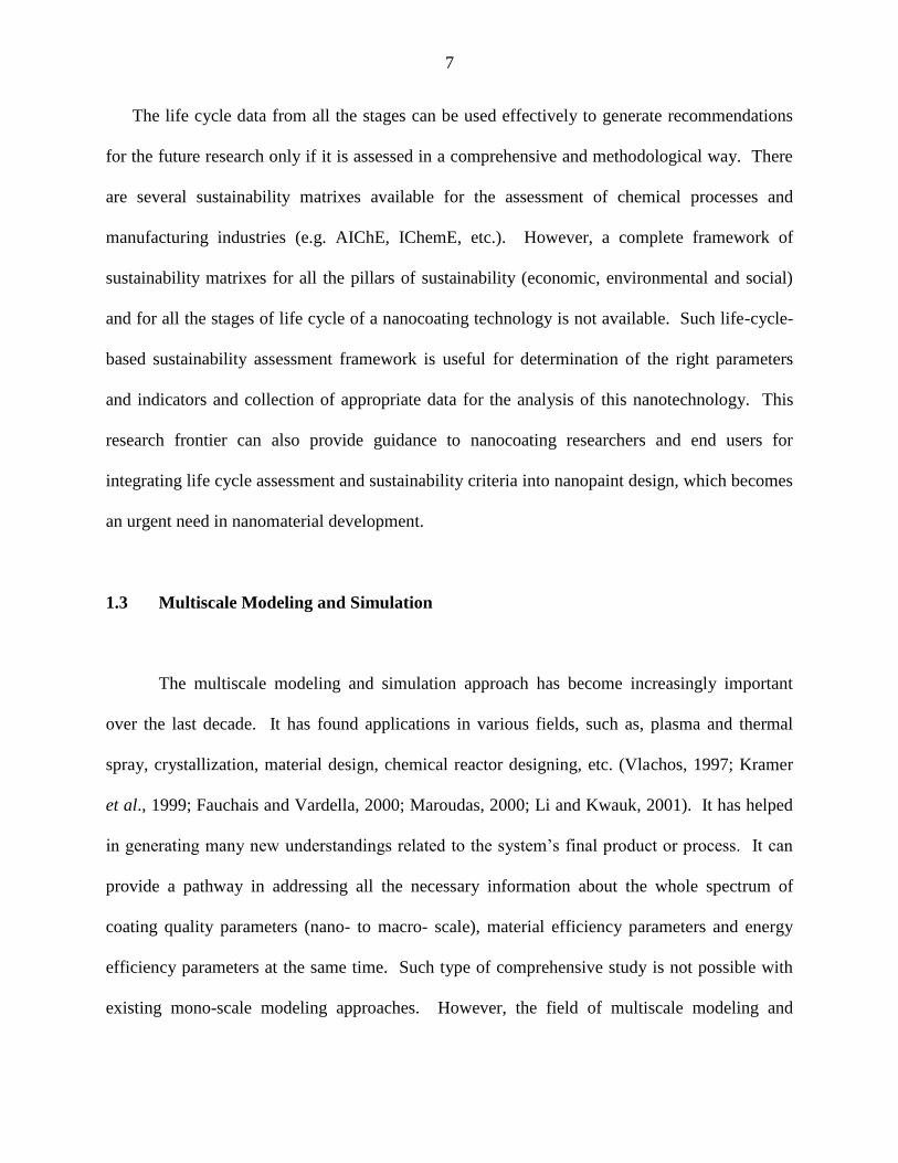
The life cycle data from all the stages can be used effectively to generate recommendations
for the future research only if it is assessed in a comprehensive and methodological way. There
are several sustainability matrixes available for the assessment of chemical processes and
manufacturing industries (e.g. AIChE, IChemE, etc.). However, a complete framework of
sustainability matrixes for all the pillars of sustainability (economic, environmental and social)
and for all the stages of life cycle of a nanocoating technology is not available. Such life-cycle-
based sustainability assessment framework is useful for determination of the right parameters
and indicators and collection of appropriate data for the analysis of this nanotechnology. This
research frontier can also provide guidance to nanocoating researchers and end users for
integrating life cycle assessment and sustainability criteria into nanopaint design, which becomes
an urgent need in nanomaterial development.
1.3 Multiscale Modeling and Simulation
The multiscale modeling and simulation approach has become increasingly important
over the last decade. It has found applications in various fields, such as, plasma and thermal
spray, crystallization, material design, chemical reactor designing, etc. (Vlachos, 1997; Kramer
et al., 1999; Fauchais and Vardella, 2000; Maroudas, 2000; Li and Kwauk, 2001). It has helped
in generating many new understandings related to the system‟s final product or process. It can
provide a pathway in addressing all the necessary information about the whole spectrum of
coating quality parameters (nano- to macro- scale), material efficiency parameters and energy
efficiency parameters at the same time. Such type of comprehensive study is not possible with
existing mono-scale modeling approaches. However, the field of multiscale modeling and
8
simulation requires further exploration. Since, sustainable nanocoating technology development
needs a complete understanding of microstructure, material, product and process behavior
throughout a wide range of length (10-9
– 10 m) and time (10-6
– 103 s) scales, multiscale
modeling and simulation becomes a must.
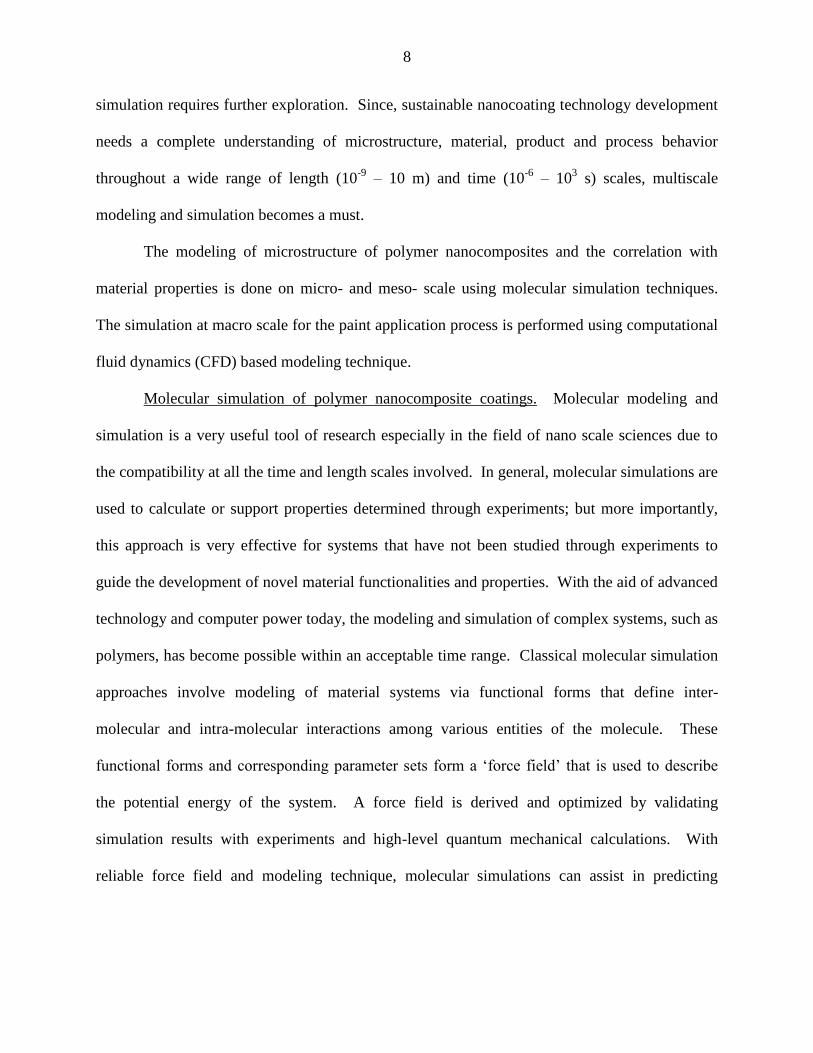
The modeling of microstructure of polymer nanocomposites and the correlation with
material properties is done on micro- and meso- scale using molecular simulation techniques.
The simulation at macro scale for the paint application process is performed using computational
fluid dynamics (CFD) based modeling technique.
Molecular simulation of polymer nanocomposite coatings. Molecular modeling and
simulation is a very useful tool of research especially in the field of nano scale sciences due to
the compatibility at all the time and length scales involved. In general, molecular simulations are
used to calculate or support properties determined through experiments; but more importantly,
this approach is very effective for systems that have not been studied through experiments to
guide the development of novel material functionalities and properties. With the aid of advanced
technology and computer power today, the modeling and simulation of complex systems, such as
polymers, has become possible within an acceptable time range. Classical molecular simulation
approaches involve modeling of material systems via functional forms that define inter-
molecular and intra-molecular interactions among various entities of the molecule. These
functional forms and corresponding parameter sets form a „force field‟ that is used to describe
the potential energy of the system. A force field is derived and optimized by validating
simulation results with experiments and high-level quantum mechanical calculations. With
reliable force field and modeling technique, molecular simulations can assist in predicting

9
various material properties and guiding experimental efforts for synthesis and characterization of
new materials.
Two most popular approaches for molecular simulation are: stochastic approach (Monte
Carlo) and deterministic approach (Molecular Dynamics). Additionally, there are several other
techniques that work at different length and time scales and sometimes combine the features of
MD and MC. The most distinctive feature of these molecular simulation techniques is their
potential to evaluate material‟s macroscopic thermodynamic properties such as internal energy,
shear and tensile modulus, pressure, coefficient of thermal expansion, heat capacities, etc.
Macroscopic properties at equilibrium are calculated using the time average of MD simulation
and the ensemble average of MC simulation. The obvious benefit of MD over MC is that it
gives route to the evaluation of transport (macroscopic) properties- also known as dynamical
properties such as transport coefficient, rheology of the system, etc. using time correlation
functions of corresponding microscopic variables. MD simulation makes use of optimized force
field parameters to predict bulk properties of the system, whereas in MC the parameters are
assumed. Hence, the simulation results obtained from MD can be applied to make comparisons
with proposed theories and experiments directly, while it is not possible with the results from
MC simulation.
Molecular dynamics simulation was first applied by Alder and Wainwright to study the
phase transition of fluids (Alder and Wainwright, 1957). Theoretically in molecular modeling,
the trajectories of particles/atoms are related to physical properties of the system by statistical
thermodynamics. MD allows the prediction of time evolution of the material. The trajectory of
positions and momenta of particles at different times can be used to evaluate all bulk physical
properties of the system. Primarily, MD consists of three constituents: (1) initial configuration
10
and velocities of all the particles of the system, (2) the interaction potentials among all the
particles, (3) trajectory of positions of the particles at different times calculated by solving
standard Newtonian equation of motion (Zeng et al., 2008). The equation of motion is usually
given as,
(t)
t (1.1)
where represents the force acting on the particle i at time t and it can be derived from the
potential energy U( ); is the position of particle i having mass mi. A physical simulation
consists of the total potential energy that is a combination of all the interaction potentials among
particles of the system, periodic boundary conditions and control of appropriate temperatures and
pressures to satisfy conditions of different thermodynamic ensembles. All the interaction
potentials together with corresponding parameter set which contribute towards total energy of the
system form a force-field. The selection of appropriate force field depends on transferability,
accuracy of parameters and total computational time. The total interaction potential can be
broadly classified into two categories of bonded interactions and nonbonded interactions (Allen,
2004). Several terms involved in these two categories that sum up to total energy can be
represented as:
U( ) ∑Ubond ( ) + ∑Uangle ( ) + ∑Utorsion ( )
+ ∑Uvdw ( ) + ∑Uelectrostatic ( ) (1.2)
where Ubond is the bond stretching energy; Uangle is angle bending energy; Utorsion is the dihedral
angle energy; Uvdw is the van der Waals energy; and Uelectrostatic is the electrostatic energy. The
bond and angle terms, Ubond and Uangle, do not allow covalent bonds to break. The torsion energy
term, Utorsion, usually consists of two types of potentials: dihedral angle potential and improper
potential. The former term is included to constrain the rotation of molecule around the specific
11
bond and the later term is used to maintain the planarity of atoms. The non-bonded terms, Uvdw
and Uelectrostatic, are more computationally expensive because of the higher number of interactions
involved. At the start of the simulation, atoms/particles are assigned initial velocities which
contribute towards total kinetic energy of the system. This kinetic energy is dictated by the
temperature of the system. Using the forces on each particle and temperature of the system, the
acceleration of each particle can be determined.
Integration of all the equations of motion for the system yields to the formation of a
trajectory having detailed information about positions and velocities of all the particles, total
internal energy and temperatures and pressures of the system at different points of time. The
integration of equations of motion over long time may be tedious and very complex at times.
These equations can be integrated through many available algorithms using finite difference
methods. All the available integration algorithms assume that the positions, velocities and
accelerations of the particles can be approximated using Taylor series expansion.
The selected algorithm must comply with the characteristics of the equations of motion as
given below.
(i) The selected algorithm must deal with short or long time-scales involved in the
simulation.
(ii) The calculation of forces is mathematically expensive and time consuming. Thus,
it should be performed at a frequency as low as possible.
(iii) The updating of atomic coordinates must follow calculation of dynamic properties
accurately and assist sampling of correct ensemble.
(iv) The algorithm should also favor large time steps and thus they should not involve
storage of large derivatives of positions and velocities.
12
The algorithm of Verlet satisfies most of these requirements. Commonly used algorithms
in MD simulations are velocity verlet and leapfrog (Rapaport, 2001; Hairer et al., 2003). The
Verlet algorithm calculates the position t+ t and acceleration a t+ t of the particle at a time
t+ t by using the position ( ) and acceleration ( ) at present time t and the position of
particles t- t at time t- t. Whereas, in Leapfrog algorithm, the velocities are calculated at first
at time t+
t and these are used to calculate positions of particles at time t+ t.
In case of polymers, the system size is very large. Most of the times the surface effects of
the polymer with simulation box surface are neglected. In such cases periodic boundary
conditions (PBC) are employed on the simulation box. It considers an infinite space filled with
an array of exact replicas of the constructed simulation region. PBC comes with some
consideration to satisfy periodicity. It assumes that an atom leaving the simulation box through a
particular wall immediately re-enters the region from the opposite end. The interaction of one
atom with another atom at a distance rc within the box is same as that of the atom present at the
same distance in the adjacent replica of the box. These constraints must be taken into account
while dealing with equations of motion and new positions of atoms after each integration step.
After each step, the atoms moving out of the boundary of the box must be brought inside from
the opposite side and the coordinates must be adjusted accordingly. Evidently, PBC are most
easy to handle in case of regions of rectangular dimensions; although it is not an essential
requirement.
MD simulation can be carried out in many different ensembles. Ensemble is a collection
of systems with different microscopic states but same macroscopic and thermodynamic states.
Most common ensembles include microcanonical (NVE), canonical (NVT) and grand-canonical
(µVT) where µ is a chemical potential. Sometimes in practice, simulations need to be performed

13
at a constant temperature or pressure condition. The methods to incorporate these isothermal and
isobaric conditions consist of restructuring of Lagrangian equations of motion. Some of the
recognized methods for temperature control are Nosé-Hoover thermostat, the Berendson
thermostat and Langevin dynamics. The methods for pressure control are the Berendson pressure
bath coupling, Langevin piston method, etc.
Macroscale modeling using computational fluid dynamics. Nanopaint application using
paint-spray technique is a complex multiphase system. The paint material is composed of resin,
pigment, additives, solvents and nanoparticles. During the spray application substantial amount
of solvents are released into the atmosphere in the form of volatile organic content (VOC) and
the nanoparticles are released along with the paint droplets. Inside a spray booth, the excess of
paint which does not get deposited on the substrate panel is removed by ventilation air passing
through the booth ambience. In order to model this paint-spray process, multiple components
and fluid phases need to be analyzed carefully and with precision. A successful design of the
process depends on the accurate prediction of the interactions (chemical, mechanical and
thermal) between these phases. Since this process is impossible to observe at a micro level, one
has to rely on numerical modeling and simulation to gain insights into improving the process
performance, environmental emissions, safety and reliability.
Numerical simulation can play an important role in analyzing such complex system
problems. A discipline of computational fluid dynamics studies the numerical simulations and
the solutions for the equations of motion of fluids. Computational Fluid Dynamics (CFD) is the
science of predicting fluid flow, heat and mass transfers, chemical reactions, and corresponding
phenomena by solving the equations governing these processes using a numerical process. It

14
provides a wide variety of methods for simulating the fluid flow problems. Through CFD, a
qualitative and quantitative prediction of fluid flows can be made by means of
Mathematical modeling (partial differential equations),
Softwares and tools (various types of solvers and tools for pre- and post- processing
of the system),
Numerical methods (discretization and solution techniques).
CFD calculations are based on the first principles of mass, momentum and energy
conservation. CFD modeling is capable of providing a detailed description of fluid flow
variables, velocity, temperature and mass concentration profiles anywhere in the flow regime.
Such details may not be possible to obtain from physical models and systems. In CFD modeling,
the fluid flow region is divided into numerous small elements within which the flow is either
kept fixed or varies smoothly. The equations of mass, momentum and energy balances are
represented in terms of variables at the predetermined positions inside the elements. The
solutions of these equations are evaluated until it reaches the required accuracy.
The working and use of CFD requires a basic set of steps to be followed. These steps are
given below.
1. The physical problem to be studied should be defined.
2. The physical system should be designed by defining its geometry in either 2D or 3D
space.
3. The conservation of mass, momentum and energy should be satisfied throughout the
system‟s region under consideration.
4. The properties of fluids involved in the system are modeled empirically.

15
5. Assumptions are made to simplify the problem and make it tractable (e.g. steady-
state, transient, compressible, 2 dimensional, etc.).
6. Appropriate initial and final boundary conditions should be provided.
7. The system domain is discretized into a finite number of volumetric regions, called
cells or grids. The discretized area is called the “mesh”.
8. The governing equations for mass, momentum and energy conservation are applied
on the mesh and individual cells through numerical methods of discretization.
9. The post-processing of the solution is carried out to obtain the results for desired
quantities (e.g. heat flow, mass fraction, temperature, drag, separation, pressure
gradient, etc.).
The foundation for modeling of the fluid flow is provided by Navier-Stokes and
continuity equations. The Navier-Stokes equations can be derived by the dynamic equilibrium of
fluid elements. For compressible flow, the governing equations are the continuity equation,
momentum equation (Navier-Stokes) and the energy equation.
The continuity equation is given as,
0
z
)w(
y
)v(
x
)u(
t
(1.3)
The Navier-Stokes equations are given as,
xFz
u
y
u
x
u
x
p
z
uw
y
uv
x
uu
t
u
2
2
2
2
2
2
(1.4)
xFz
v
y
v
x
v
x
p
z
vw
y
vv
x
vu
t
v
2
2
2
2
2
2
(1.5)
xFz
w
y
w
x
w
x
p
z
ww
y
wv
x
wu
t
w
2
2
2
2
2
2
(1.6)

16
The energy equation is given as,
z
Tk
zy
Tk
yx
Tk
xz
Tw
y
Tv
x
Tu
t
Tcp
z
pw
y
pv
x
pu
(1.7)
where Φ is the dissipation function, u, v and w are the velocity components in x, y and z
directions, ρ is the density, p is the pressure, T is the temperature, cp is the specific heat at
constant pressure and μ is the viscosity.
The continuity equation represents the law of conservation of mass and thus must be
satisfied at each point in the fluid region. In Navier-Stokes equations (Eqs. 1.4-1.6) the terms on
the left hand side represent the inertial term which arise from momentum change. This term is
compensated by the pressure gradient
x
p, the viscous forces and the body forces (Fx).
The importance of accuracy in multiphase modeling of sprays and droplets in various
engineering applications is well known (Sirignano, 1999; Sazhin, 2006). Especially in the case
of paint spray system, the model needs to take care of complicated fluid dynamics, multiple
phases, heat/mass transfer, evaporation and deposition etc. In order to study all the
characteristics of the coating, the application process of the paint material must be reproducible
and well-controlled. With all the functionalities and abilities of CFD-modeling, it can provide a
detailed view of the process, and study the effects of different operating conditions and
geometries by simulating the corresponding flow behavior. It can offer significant insights into
the coating process and show how the changes in workplace geometry, operating conditions,
material type and application pattern can affect the quality of coating and performance of the
system. With accurate modeling of this painting process, one can expect a number of

17
advancements in the understanding of the spray painting related issues, such as environmental
emissions, paint transfer efficiency, coating quality, uniform film deposition, solvent
evaporation, defects, and safety measure by assessing workers‟ exposure to overspray paint,
VOC, nanoparticles, etc. as a function of spray booth structure and ventilation system.
1.4 Towards Sustainable Nanocoating Technology Development
Nanotechnology, as a result of all the possible opportunities it provides for innovation, is
finding innumerable ways to enter human‟s life. It offers a promise to provide breakthrough
technologies for a number of industries and consumer sectors with improved and novel
functionalities and with a reduction in consumption of hazardous materials, consumption of
energy as well as generation of wastes. Paint technology is no exception in accepting the ever
increasing dominance of nanotechnology based products over conventional products. In fact, a
number of nanotechnology based consumer products of paints and inks are already available in
the market. However, the implications of nanomaterials and products on the environmental
safety and human health are often either ignored or not highlighted. There is a major knowledge
gap existing between the applicability of nano-size materials into consumer products and their
effects on health and environment.
Nanomaterial is referred as a material with at least one component in the order of 1-100
nanometers. These materials can be individual nanoparticles of different shapes or aggregates of
several nanoparticles together. In case of coating application there are numerous types of
nanoparticles that are incorporated into polymer resin to synthesize final nanocomposite
coatings. These nanoparticles include TiO2, SiO2, Ag, MMT clay, aluminium oxide, zinc oxide,

18
etc. They introduce improved and newer characteristics into nanocomposites such as improved
mechanical, thermal, dielectric properties, biodegradability, anti-corrosion, self-cleaning, dirt
repellency, anti-bacterial, etc (Zhang et al., 2005; Nobel et al., 2007; Chen et al., 2008).
Presumably, this type of revolutionary technology should be sustainable in terms of economy,
resource and energy efficiency and health care. However, so far only the economic prospect of
nanotechnology has been highlighted and a very little attention is given to its social and
environmental implications (Linkov et al., 2007; Dhingra et al., 2010). Its potential to develop
systems with smart and newer functionalities significantly inspires competitiveness among
different companies which use nanotechnology based coatings to avail all its economic benefits.
Currently, the economic growth of the nanocoatings market and corresponding research and
development gives a very little attention to assessment of social and ecological risks which are a
part of complete holistic sustainability assessment of nanocoating products. Thus, it is important
to stress on benefits and risks of this technology during the life cycle to detect all hidden short
and long term adverse effects and to support all the decisions related to its future development.
A holistic view for a sustainable development of nanocoating technology is represented in Figure
1.1.
Figure 1.1. Holistic view of sustainability.

19
A comprehensive study on the life cycle of nanoproducts can analyze, evaluate and
address all the issues related to the environmental and health effects of nanoparticle induced
coating materials. The life cycle based study, as proposed by EPA, considers all the stages of
nanocoating‟s life from “cradle-to-grave” which include, (1) material selection, (2) system‟s
design, (3) use and maintenance, (4) recycling and reuse, and (5) disposal.
Figure 1.2 broadly classifies these various stages of nanopaint life with applicable EPA
regulations.
Figure 1.2. Life cycle of a nanopaint-nanocoating system
In general, it is very challenging to perform complete sustainability assessment of
emerging or developing technologies (e.g. nanocomposite coatings) due to insufficient data
availability for inputs and outputs of the system at each stage of life cycle. However, if
succeeded, it can provide significant amount of supplementary information to support decisions
related to the future development. LC based sustainability assessment can provide answer to the
questions such as,

20
How the performance of nanocoating is compared with conventional coating over its
life-cycle?
How much energy efficiency is accomplished by incorporating nanoparticles into
conventional products?
Which stage of life cycle dominates the energy consumption?
Which stage of life cycle is most prone to the release of nanomaterials in the
environment?
What are the toxicity issues involved with released nanomaterials at different phases
of life cycle?
What is the impact of nanoparticle coatings compared to those of conventional paint
products on geographical parameters?
How is the end-of-life management of nanopaints compared to that of conventional
paints? Is there a way for reuse or recycling?
The answers to these questions and development of a comprehensive life-cycle based
sustainability assessment methodology for analysis of nanocoating technology can significantly
assist in directing the research and sustainable development of these paint products.
1.5 Main Goals and Scientific Contributions
The objective of this research is to develop a comprehensive multiscale design and
development tool to aid the development of sustainable nanocoating technology which can
deliver products with multiple functionalities. The challenge to this research comes from the
lack of thorough knowledge about the vast and complex microstructure, huge design space and

21
substantially limited data availability. The existence of vast design parameters and experimental
complexity makes nanopaint design optimality extremely difficult to address if not impossible.
Thus, the focus of research on nanocoating technology is being shifted towards the optimal
design formulation of nanocoatings, where the need for computational modeling and simulation
methodologies is inevitable. In silico experiments using computational material designs of
nanocoating resins have immense potential to facilitate identification of important correlations
among material, structure, property and performance. It can assist the scientific research for the
development of more sustainable multifunctional nanocoatings, the application methodologies
and product design.
In order to meet the goal of developing a methodology to aid the research on sustainable
nanocoating materials, we integrate the top-down, goals/means, inductive systems engineering
and bottom-up, cause and effect, deductive systems engineering approaches, as shown in Figure
1.3 (McDowell and Olson, 2008), and develop a complete multiscale framework which can
define a correlation among material-structure-property-performance. Previously, through top-
down approach, the nanocoating system was studied by using modeling and simulation at meso-
and macro-scales of length and time (Xiao et al, 2007; Xiao et al., 2010; Xiao and Huang, 2009).
This research focuses on bottom-up approach to develop nano- and micro-scopic models and
connect it to the already developed mesoscopic modeling methodology to complete the
multiscale materials development framework.

22
Figure 1.3. Multiscale modeling framework integrating top-down
and bottom-up systems engineering approaches (McDowell and Olson, 2008).
For the process, product design and mesoscale development of paint material, the models
based on CFD simulation technique and multiscale Monte-Carlo based simulation technique
have been developed (Xiao et al, 2008; Xiao and Huang, 2009; Xiao et al., 2010; Xiao et al.,
2010). The CFD based modeling provides crucial knowledge about paint film application
technique and operating parameters related to paint spray and curing, and the Monte Carlo based
modeling provide intrinsic relationship among nanopaint components and bulk properties
through development of coarse-grained (CG) freely jointed bead-spring structures. Although,
the bead-spring model is useful to understand the correlation between coating microstructure and
bulk properties, it lacks the details from specific chemistry of polymers. Thus, the properties of

23
nanoparticle-induced coatings with different materials of resin cannot be studied. This chemical
specificity can be provided through structure and thermodynamics based coarse-grained
modeling. In this work, via bottom-up approach, we develop chemistry-specific CG nanocoating
material designs and integrate it with the previous accomplishments to produce a complete
multiscale framework that can lead to the development of optimal multifunctional nanocoating
formulation using assessment of the correlation of material-property-product-processing.
The introduction of unique and improved properties of the paint material through
nanotechnology may also have environmental and societal implications which may lead to
greater risks to human health and safety. Thus, the environment, health and safety impact
assessment of existing and emerging nanocoating materials has become a serious issue. In this
research, a life-cycle-based sustainability assessment framework is developed for the
nanocoating technology which can highlight the potential problems that this technology may
cause to the environment, society and economy. For the assessment, five stages of cradle-to-
grave life-cycle of a paint material (material selection, paint manufacturing, paint spray/flash,
curing and end use) have been considered. Based on the data available from literature, research
papers, industries and computational models related to paint technology, individual sets of
parameters have been identified for each stage of the life-cycle which aid to the overall
sustainability assessment of each stage. The sustainability indicator matrices for each stage
encompass all the aspects concerning the economic benefits, environmental issues and societal
impact of that stage. Using case studies of automotive coating systems, the assessment results
are combined together and analyzed to identify critical parameters which influence the overall
nanopaint technology sustainability. The analysis of each stage of the life cycle using
sustainability aspects and developing a correlation among different parameters and indicator

24
matrices related to environmental, social and economic aspects can significantly direct the future
development of these products towards sustainability.
1.6 Organization of Dissertation
The dissertation body is mainly composed of two sections. The first section describes the
multiscale computational modeling effort for polymer-nanocomposite coatings study and the
second section focuses on the development of life-cycle based sustainability assessment
framework and paint process modeling to obtain the data for the assessment.
In Chapter 2, the multiscale computational design of nanopaint is developed. The
nanopaint is modeled on atomistic level by using CHARMM force-field. It is then mapped onto
the coarse-grained structure which is developed by applying MARTINI force field protocols.
The developed coarse-grained system is then used for the study of effects of different sizes,
volume fractions and distributions of nanoparticles and the polydispersity of polymer resin on
the structure-property correlations and interfacial behavior of resin molecules. In Chapter 3, the
efforts made towards the experimental verification of multiscale computational design of
nanopaint are described. As a case study, the polymer nanocomposite films are synthesized by
layer-by-layer application of acrylic resin and TiO2 nanoparticles dispersion. These films are
characterized and tested through experimental analysis techniques such as XRR and AFM to
determine the change in the mechanical stiffness of the films after addition of different
dispersions of nanoparticles.
The later Chapters are focused on the development of life-cycle based sustainability
assessment (LCSA) methodology and the macroscale modeling of paint application process to
obtain the data for nanocoating technology assessment. In Chapter 4, a comprehensive LCSA
25
methodology is described. The parameter sets and corresponding sustainability indicator
matrixes are developed for each of the 5 stages of life-cycle which include material selection and
preprocessing, paint manufacturing, paint application and curing, use and disposal. The
applicability of the methodology is demonstrated with a case study on a set of coating systems
assessment. Chapter 5 and Chapter 6 provide the details of the modeling and simulation of paint
application process (automotive paint-spray). The modeling of paint-spray technique is
performed in order to study the effects of nanoparticles addition into coating matrix on the
environmental emissions inside the spray-booth and coating film quality parameters. The
topological characteristics of the paint film are also studied by developing case studies of various
paint spray patterns and application parameters. The data obtained in these chapters could be
used for the quantification of some of the sustainability indicators described in Chapter 4.
Finally, the concluding remarks and possible directions to extend this work in the future
are outlined in Chapter 7.

26
CHAPTER 2
MULTISCALE MODELING AND ANALYSIS OF POLYMER
NANOCOMPOSITE SYSTEMS
With the advancement of computing power, it is evident that computational modeling
tools are going to accelerate the development of nanocomposite coating technology for all the
superior properties achievable. The ability of having a complete control on nanocoating
microstructure and complex behavior of polymer matrix makes the research using computational
methods more significant. However, it is the selection of appropriate modeling techniques and
mathematical algorithms that ensures the generation of meaningful information out of
simulation. Nanopaints being materials with applications at continuum level and properties
defined by microstructures, it is critical to generate intrinsic correlations among coating‟s
material, structure, property and performance.
2.1 Objective and Significance
It has been proven that the interface between polymer and nanoparticle plays a key role in
introduction of superior and newer functionalities into nanocoatings. Besides the interface, the
chemical nature of polymeric material, type and morphology of nanoparticles are amongst other
important parameters to bring along the property enhancement. An extensive experimental study
is underway to determine all critical factors responsible for these superior properties as well as
27
newer functionalities of nanocomposite coating matrices. The enhancement of mechanical and
rheological properties of polymer nanocomposites is demonstrated by addition of different types
of nanoparticles such as MMT clay, silica, TiO2, etc. into polymer resins (Van Hamersvelt et al.,
1999; Tigli and Evren, 2005; Chow and Mohd Ishak, 2007; Nobel et al., 2007; Chen et al.,
2008). A work is also in progress to bring-in newer functionalities like self-cleaning and smart
corrosion resistance into coating materials (Zhang et al., 2005; Radhakrishnan et al., 2009).
Despite of growing knowledge about nanocomposite coatings through experiments, there
are several structure and property correlations that are unanswered and still being investigated.
With the development and availability of computing power, computational modeling and
simulation has become a very useful tool to study and address these issues. Over the years,
simulation techniques are developed and applied to various systems such as polymers and
biomolecules at multiple scales of length and time ranging from nanoscopic to macroscopic
continuum levels. Simulations on atomistic level provide chemical specificity to molecular
models using empirically verified and generic force fields. But the design complexity and huge
design space of polymer melts at atomistic level brings along several limitations of time and
length scales. It is presently very difficult to model the behavior of polymer melt around
nanoparticles at atomistic levels that requires tens of microseconds of time at tens of nanometers
of length for equilibration.
Coarse-graining approach can help in overcoming this limitation of atomistic modeling.
Kremer and Grest proposed the popular bead-spring model for simulation of long chain
molecules (Kremer and Grest, 1990). It has been applied for CG modeling of large molecules
like polymers by several research groups (Starr et al., 2002; Smith et al., 2003; Kalra et al.,
2010; Xiao et al., 2010). Although the bead-spring model is applicable for understanding the

28
science behind polymer-nanoparticle surface interaction leading to superior properties, it lacks
the details from specific chemistry of polymers. Thus, it cannot be applied for studying the
properties of coating with different materials of polymers. This leaves a clear gap between two
scales of simulation and makes it almost impossible to develop a correlation between atomistic
and CG modeling. In order to incorporate chemical specificity into CG models, the development
of a structure based or thermodynamics based coarse-grained models is essential. This type of
CG modeling involves grouping of atoms from all-atom model into larger size beads. Thus, it
decreases the total number of atoms/particles in the system to be simulated. As a result of
reduced number of degrees of freedom, the CG models usually run much faster with larger time
steps during molecular dynamics (MD) simulations compared to atomistic models.
In order to prepare a comprehensive multiscale modeling tool for the study of
nanocomposite coating material, it is critical to develop a well-defined CG model of selected
polymer resin system that can be transferrable over different scales of time and length. In our
work, we adopt a thermodynamics based CG modeling technique called “The MARTINI force-
field method” which was introduced by Marrink et al. (2004). It was originally developed for
lipid bilayers and detergent molecules. Later it was extended for coarse-graining of organic
solvents, proteins and carbohydrates (Marrink et al., 2007; Monticelli et al., 2008; Lopez et al.,
2009). The applicability of the MARTINI approach for polymers has been tested and verified
over specific cases of polyethylene glycol, polystyrene and thermoset polyester coatings (Lee et
al., 2009; Rossi et al., 2011a,b). This approach consists of verification of bonded and non-
bonded parameters involved to define macromolecular structures using the data from atomistic
scale modeling. The accuracy of this model can be shown by comparing the structural and

29
thermodynamic properties such as radii of gyration, pair distribution functions, etc. with that
from all-atom models.
A significant attention is being given towards the development of water-based nanopaint
resin systems to meet continuously increasing demand for low VOC and environmentally
friendly materials. Acrylic coatings are water-dispersible and have applications in many
different types of coatings. Consequently, a research focus is gradually shifting towards
developing optimal formulations of nanocoatings that have acrylic-based resins. Needless to say
that the contribution from molecular simulation can be significant in the developmental studies
of these types of nanocoating materials due to a large number of complex structural features
involved. For this purpose, a multiscale model of an acrylic nanocomposite material is required.
Previous accomplishments of Dr. Huang‟s group covered the modeling and simulation of
nanocoating material on the mesoscopic level. In order to build a complete multiscale modeling
framework which can generate crucial information about nanocoating‟s material-structure-
product-process correlation, the simulation on the finer level is required. The nanoscopic and
microscopic simulations then need to be bridged to the previously developed mesoscopic
methodology to accomplish the objective of development of a comprehensive multiscale
modeling framework for the study of nanocoating technology. This major task involves five
distinct steps of simulation work which are to be covered.
1. Generation of the atomistic model of an acrylic polymer system using a wisely
selected force-field,
2. Development of the MARTINI parameter set to model the acrylic polymer at CG
level and verifying it using atomistic simulations and experimental data,
3. Incorporation of nanoparticles of selected size and morphology.

30
4. Use of the final polymer-nanocomposite model to predict structural features and bulk
properties of the nanocoating material and to explore critical parameters that
contribute towards enhancement of the material performance.
5. Building a bridge between MARTINI-based simulation model and previous Monte
Carlo-based simulation model.
After accomplishing the objective to develop a multiscale molecular modeling
methodology to simulate a polymer-nancomposite coating, it can be very useful to learn and
discover new knowledge about the microstructure-property-performance correlation among paint
resin and dispersed nanoparticles. It can help experimentalists to prepare optimum formulations
with controlled enhancement in target properties. The findings from life-cycle based
sustainability assessment work can be employed easily to predict property changes of the coating
material with accuracy and with lower cost and time.
2.2 Atomistic Modeling
The optimization of MARTINI force field parameters significantly relies on accuracy of
atomistic modeling. The atomistic modeling uses data from generic force-fields for simulation
of molecules. By selecting appropriate force field, atomistic simulation is capable of predicting a
number of structural and thermodynamic properties of a molecular system. In case of polymeric
material the size of the system, length and number of polymer chains and number of atoms in the
system decide the time required for equilibration under given conditions of ensemble. Usually
the time step for this simulation is very small. The validity of the atomistic model is justified by

31
reproducing empirical polymer melt densities and certain structural properties such as radii of
gyration, mean squared distances, etc.
2.2.1 Force Field Selection and Optimization
The selection of appropriate force field depends upon several factors such as the quality,
applicability to the selected molecular structure and ability to predict target properties with
accuracy. The force field stores all the necessary information for the calculation of forces and
energies. Typically the force field should consist of following information: (i) atom types, (ii)
partial atomic charges, (iii) functional forms of equations to represent energies, (iv)
corresponding parameter values needed for all functional equations, (v) rules to generate new
parameters for molecules that are not explicitly defined, and (vi) ways of assigning different
types of functional forms and corresponding parameters.
The basic functional form expressing total energy of the system forming the force field is
the sum of bonded (covalently) interactions and nonbonded interactions (Van der Waal‟s and
electrostatic interactions). The bonded energy, Ebonded, generally accounts for bond stretching
(Ebond), angle bending (Eangle) and dihedral torsion (Edihed) terms.
Ebonded= Ebond + Eangle + Edihed (2.1)
The nonbonded energy, Enonbonded, accounts for Van der Waals (Evdw) and electrostatic
(Ecoulomb) interaction terms.
Enonbonded= Evdw + Ecoulomb (2.2)
The acrylic polymer selected for this work is polymethyl methacrylate (PMMA). There
are several classical force fields that are suitable for the simulation of PMMA model. These

32
include CHARMM, AMBER, CVFF, COMPASS and PCFF. The force field selected for
atomistic modeling of PMMA is an extension of CHARMM (Chemistry at HARvard
Macromolecular Mechanics). CHARMM was originally developed by Dr. Alex MacKerell
(Feller et al., 1997; Guvench and MacKerell, 2008). It was parameterized on the basis of ab-
initio and experimental data on energies and geometries of small organic molecules, vibrational
spectra and torsional rotational surfaces.
There are several different versions of CHARMM that are released till date. The most
commonly used are CHARMM19 (Feller et al., 1997), CHARMM22 (MacKerell et al., 1998)
and CHARMM27 (Foloppe and MacKerell, 2000). In CHARMM force-field, potential energy
functions for bonded interactions are expressed as harmonic potentials. The total bonded energy
term can be written as:
e ∑ ( - )2
∑ ( - 0)2
a le ∑ (1 cos( - ) ) e al
∑ ( - )2
e ∑ ( - )2
U e - a le (2.3)
where the first term represents harmonic bond potential and Kb and b0 are the force constant and
equilibrium bond length respectively. The second term in the equation stands for the harmonic
angle potential where K and 0 denote angle constant and equilibrium angle in degrees. The
third term accounts for the dihedral angle potential with torsional force constant , dihedral
angle in degree, n is the multiplicity and δ is the phase shift. Impropers are used to restrict the
molecular geometry. This fourth term corresponds to out of plane bending where is the
stiffness with equilibrium angle . The fifth Urey-Bradley potential term accounts for
interaction between the 1st and 3
rd atom, separated by two harmonic bonds, where is the force
constant and u0 is the equilibrium distance between 1, 3 atoms in the harmonic potential.

33
The nonbonded potential functions are represented by the standard 12-6 LJ potential and
electrostatic interactions as shown below:
e ∑ e a
[(
)
- 2 (
)
]+ ∑
e
a
(2.4)
where the first term accounts for van der Waals force of interaction between a pair of atoms
represented by the 12-6 LJ potential. is the equilibrium distance between two atoms at a
point where the LJ potential becomes zero. The last term stands for the electrostatic force of
interaction between atoms with partial atomic charges (MacKerell et al., 1998).
Figure 2.1 shows the proposed PMMA repeating unit model which is used in all the
atomistic simulations. The molecular weight of each repeating unit of PMMA is 100 g/cm3.
Figure 2.1. PMMA repeating unit.
Partial atomic charges. CHARMM27 does not have an optimized set of partial charges
directly applicable to PMMA molecules. Thus, partial charge on each atom of a PMMA
repeating unit is determined using the CHELPG (charges from electrostatic potentials using a
grid based method) type of atomic charge calculation scheme. Each PMMA chain was
constructed with three types of residues, which are the derivatives of a molecular structure
formed by capping both ends of the methyl methacrylate monomer with methyl groups. The

34
geometry of the PMMA monomer was optimized using Hartree Fock (HF) theory and 6-
31G+(d,p) basis set. Calculations were started from a variety of initial conformations to ensure
the optimized state corresponded to the global energy minimum (Breneman and Wilberg, 1990).
This optimized geometry was used for the determination of partial charges via the CHELPG
method (Breneman and Wilberg, 1990). The partial atomic charges on each atom of a PMMA
repeating unit formed by two different intial conformations are given in Table 2.1.
Conformation 2 led to the minimum energy of the optimized state of the system as compared to
that obtained from Conformation 1. Thus, the corresponding set of charges was selected for
further calculations.
Table 2.1. Partial atomic charges on MMA unit obtained after Gaussian calculations
Atom name Partial charges with
Conformation 1
Partial charges with
Conformation 2
C1 -0.20 -0.12
C2 0.09 0.16
C3 -0.15 -0.23
C4 0.88 0.87
C5 -0.12 -0.02
H1 0.07 0.01
H2 0.07 0.01
H3 0.04 0.05
H4 0.04 0.05
H5 0.04 0.05
H6 0.05 0.08
H7 0.05 0.08
H8 0.05 0.08
O1 -0.64 -0.65
O2 -0.51 -0.42
The partial atomic charges for the three residues of PMMA were derived from the
charges determined for the reference molecular structure and with 2nd
initial conformation of
atoms (see Figure 2.1). One type of residue was used to represent MMA repeat units located

35
inside each polymer chain, whereas the other two types formed capping units. The final set of
atomic charges for each residue was obtained through normalizing the atomic charges of the
structure in Figure 2.2 and by keeping the total charge on each residue equal to zero.
Figure 2.2. Partial atomic charges obtained from Gaussian after
optimization of MMA monomer capped with methyl groups.
Dihedral optimization. All the bonded and non-bonded potential parameters for PMMA
modeling were obtained from CHARMM27 force field developed for lipid molecules. Getting
the non-bonded parameters for new molecules with the use of analogy to previously
parameterized molecules can often be well assigned. However, the bonded parameters are
capable of posing more difficulty as the possibility of having unparameterized connectivity
among atoms become larger for bonds, angles and dihedral angles (Guvench and MacKerell,
2008). In case of PMMA, though it was possible to get the parameterized connectivity of bonds
and angles, the dihedral potentials still needed to be optimized. It was achieved by using
CHARMM general FF optimization methodology (Guvench and MacKerell, 2008;
Vanommeslaeghe et al., 2010). Typically the target data selected for fitting the dihedral angle
36
potentials are energies from QM (quantitative mechanical) adiabatic potential energy scans. For
a dihedral angle A-B-C-D, a relaxed potential energy scan is done by rotation about the bond B-
C over 360 degrees at fixed increments in QM representation. The same scan is also done in the
MM (molecular mechanics) representation by using all-atom CHARMM force field dihedral
parameters to be optimized. Rotational energy barrier plots are then obtained by subtracting the
potential energy of the lowest energy conformation from all higher energy conformations at
remaining angles. The set of force field parameters that would give an exact match between the
plots of rotational energy barriers from QM and MM are chosen for the selected dihedral A-B-C-
D.
For optimization of the PMMA structure, we selected two dihedral angles. One dihedral
was selected along the main chain backbone (C2-C1-C2-C3) and the other along the side chain
of PMMA (C2-C4-O2-C5) to ensure optimization over the complete PMMA structure. In order
to obtain potential energy scans at QM and MM levels, a trimer of PMMA was selected with
both chain ends capped with hydrogen atoms. The selection of a trimer structure instead of a
dimer ensured mimicking the behavior of monomers located in long chains where the
corresponding dihedral angles would encounter steric hindrance during rotation over 360
degrees. Thus, it was possible to extract accurate rotational energy barrier values which were
higher as a result of steric hindrance from neighboring monomers. Note that rotational energy
barrier values of dihedral angles from dimer structure were smaller compared to that of trimer
structure. The potential energy scans at QM level were performed by optimizing the trimer
structure at each dihedral increment with HF/6-31+G(d) level of theory calculations. Whereas at
MM level, potential energy scans were obtained over both dihedrals by optimizing the trimer
structure using the CHARMM force field set of parameters to be optimized. The molecular

37
simulation package used for performing MM level scans was CHARMM, version 34. The trimer
structure was equilibrated at each increment of rotation and final rotational energy barrier plots
were obtained. Figure 2.3 shows both dihedrals of trimer structure selected for potential energy
scans. Figures 2.4a and b represent the final match of rotational energy barrier plots from QM
and MM level calculations for both dihedrals C2-C1-C2-C3 (along the backbone) and C2-C4-
O2-C5 (along the side chain) using optimized parameters for PMMA.
The graphs of rotational energy barriers show that minimum energy conformations are
observed at ±60 degrees of dihedral angle C2-C1-C2-C3 and ±180 degrees of dihedral C2-C4-
O2-C5. Figure 2.5 shows these stable conformations of PMMA trimer which should appear with
highest probability in atomistic simulation trajectories. The final optimized set of CHARMM
force field parameters of bonded and nonbonded interactions for modeling of PMMA are given
in Table 2.2.
Figure 2.3. PMMA trimer used for determination of rotational
barriers for C2-C1-C2-C3 and C2-C4-O2-C5 dihedrals.

38
Figure 2.4. Rotational energy barriers predicted by QM and
MM calculations for dihedrals (a) C2-C1-C2-C3,
(b) C2-C4-O2-C5, (c) C2-C1-C2-C3 and (d) C2-C4-O2-C5.
Figure 2.5. Minimum energy conformations for the PMMA trimer with:
(a) dihedral C2-C1-C2-C3 fixed at -60 degrees, and
(b) dihedral C2-C4-O2-C5 fixed at 180 degrees.
(a) (b)

39
Table 2.2. CHARMM force-field parameters
for the modeling of PMMA.
(a) Bond parameters
Bond K0 Bond length
(b0)
C1-H1 309.0 1.111
C1-H2 309.0 1.111
C2-H3 322.0 1.111
C2-H4 322.0 1.111
C2-H5 322.0 1.111
C5-H6 322.0 1.111
C5-H7 322.0 1.111
C5-H8 322.0 1.111
C1-C2 222.5 1.538
C2-C3 222.5 1.538
C2-C4 200.0 1.522
C4-O2 150.0 1.334
C4-O1 750.0 1.220
O2-C5 340.0 1.430
(b) Angle parameters
Angles K 0 Kub S0
H1-C1-H2 35.50 109.0 5.40 1.802
H1-C1-C2 35.50 109.0 5.40 1.802
H3-C3-H4 35.50 108.4 5.40 1.802
H3-C3-H5 35.50 108.4 5.40 1.802
H6-C5-H7 35.50 108.4 5.40 1.802
H6-C5-H8 35.50 108.4 5.40 1.802
H7-C5-H8 35.50 108.4 5.40 1.802
C2-C3-H3 33.43 110.1 22.53 2.179
C2-C3-H4 33.43 110.1 22.53 2.179
C2-C3-H5 33.43 110.1 22.53 2.179
C2-C1-H1 26.50 110.1 22.53 2.179
C2-C1-H2 26.50 110.1 22.53 2.179
C1-C2-C3 58.35 113.5 11.16 2.561
C1-C2-C4 52.00 108.0 n/a n/a
C1-C2-C1 58.35 113.5 11.16 2.561
C2-C1-C2 58.35 113.5 11.16 2.561
C4-C2-C3 52.00 108.0 n/a n/a

40
C2-C4-O1 70.00 125.0 20.00 2.442
C2-C4-O2 55 109 20 2.326
O1-C4-O2 90 125.9 160 2.2576
C4-O2-C5 40 109.6 30 2.2651
O2-C5-H6 60 109.5 n/a n/a
O2-C5-H7 60 109.5 n/a n/a
O2-C5-H8 60 109.5 n/a n/a
(c) Dihedral parameters
Dihedrals K n δ
H1-C1-C2-C3 0.05 3 180
H2-C1-C2-C3 0.05 3 180
C2-C1-C2-C3 2.05 3 180
C2-C1-C2-C4 0.04 6 0
C4-C2-C3-H3 0 3 0
C4-C2-C3-H4 0 3 0
C4-C2-C3-H5 0 3 0
C1-C2-C1-C2 0.20 3 0
C1-C2-C3-H3 0.05 3 180
C1-C2-C3-H4 0.05 3 180
C1-C2-C3-H5 0.05 3 180
C3-C2-C4-O1 0 6 180
C3-C2-C4-O2 0 6 180
C1-C2-C4-O1 0.02 4 180
C1-C2-C4-O2 0.43 2 0
O1-C4-O2-C5 0.965 1 180
C4-O2-C5-H6 -0.10 3 0
C4-O2-C5-H7 -0.10 3 0
C4-O2-C5-H8 -0.10 3 0
C2-C4-O2-C5 1.50 3 0
(d) Non-bonded LJ parameters
Atom Rmin/2 ,1-4 Rmin/2,1-4
C1 -0.055 2.175 -0.01 1.9
C2 -0.020 2.275 -0.01 1.9
C3 -0.080 2.060 -0.01 1.9
C4 -0.070 2.000 n/a n/a
C5 -0.080 2.060 -0.01 1.9
O1 -0.120 1.700 -0.12 1.4

41
O2 -0.152 1.770 n/a n/a
H1 -0.022 1.320 n/a n/a
H2 -0.022 1.320 n/a n/a
H3 -0.022 1.320 n/a n/a
H4 -0.022 1.320 n/a n/a
H5 -0.022 1.320 n/a n/a
H6 -0.022 1.320 n/a n/a
H7 -0.022 1.320 n/a n/a
H8 -0.022 1.320 n/a n/a
*n/a: not available
2.2.2 Polymer Matrix Simulation
All of the atomistic simulations of PMMA model were performed using optimized set of
CHARMM force field parameters. The initial configuration consists of atomic coordinates for
all of the atoms located in the simulation box. The polymer chains are placed in the simulation
box at various places. The size of the box has to be adequate enough to obtain the density of the
material comparable with the experimental value.
The PMMA initial configuration was constructed using molecular packaging software
PACKMOL (Martinez et al., 2009). The molecular topology file needed for the construction of
PMMA chains defines three residue types as explained in previous section. One residue type
represents monomer repeating unit inside each polymer chain and the other two residues are used
to patch each polymer chain at the ends. Initial model consisted of 15 atactic chains of PMMA
having 50 repeating units in each. The total number of atoms in the system were 11,280. The
chains were positioned randomly inside the simulation box. The size of the box was selected in a
way to keep the initial density of the system to 0.80 g/cm3.
42
Simulation details. The amorphous PMMA structure is designed in the simulation box
with periodic boundary conditions. The molecular dynamics package used for performing all
simulations is NAMD, version 2.8. Each input file required for NAMD stores a specific
information about the system and simulation conditions. Typically the files needed are PDB,
PSF, configuration file and parameter file. PDB (Protein data bank) file stores all the atomic
coordinates with their names and residue types. PSF file stores all topological information about
the molecule. The parameter file stores all the force field parameters for a selected molecule in
CHARMM format. The configuration file provides all the details required to carry out the
simulation at given conditions of temperature and pressure and at specified time step for
specified run time. The NAMD output stores all atomic coordinates and velocities in the DCD
file. All the information about forces and energies of the system are collected in the “log” file at
each specified timestep.
In case of PMMA melt simulation, the system was equilibrated at temperature of 500 K
and pressure of 1 atm for 40 ns in the NPT ensemble. The timestep for equilibration was 2 fs. A
cutoff of 12 A was used for the calculation of all nonbonded interactions during simulation.
Switching was kept on with switching distance fixed at 10 A. The pairlist distribution was set at
14 A. The temperature during NPT ensemble was controlled with Langevin thermostat
(damping coefficient 5 ps-1
) and the pressure was kept constant by applying Nośe-Hoover
Langevin piston pressure control. The values of piston period and piston decay were set at 100
fs and 50 fs respectively. The simulation was run for 20 ns further to extract data for
measurement of all the properties.
Atomistic simulations provided validation to the optimized set of dihedral parameters by
calculating the distributions of both dihedral angles from equilibrated trajectories. Figures 2.4 c

43
and d give the plots of normalized probability distribution of both selected dihedral angles. For
dihedral C2-C1-C2-C3, the distribution is highest at angles ±60 degrees and for dihedral C2-C4-
O2-C5 the distribution was highest ±180 degrees. These distributions indicate the appearance of
conformations having lowest rotational energy barriers with highest probability.
2.2.3 Atomistic Model Verification
The atomistic model works as a benchmark to validate CG simulation. Thus, it is
important to have this model accurately reproduce structural and thermodynamic properties of
the polymer. For the modeling of PMMA structure, the nonbonded parameters are selected
through analogy with similar molecular structures. The verification of these nonbonded LJ
parameters for PMMA model is done by calculating thermodynamical properties of PMMA and
comparing it with the empirical data.
The target properties selected for the verification were density of PMMA at room
temperature and glass transition temperature. PMMA system was initially equilibrated under
melt conditions at temperature of 500 K. It was then cooled gradually at intervals of 50 K. After
cooling, the system was equilibriated under NPT ensemble for 5 ns and further for 2 ns to
generate the data for analysis. The cooling was carried out until 150 K. The density of the
system was measured after every temperature interval by averaging over the trajectory of last 2
ns of simulation.
The density of PMMA at 300 K was found to be 1.154 g/cm3 which was in good
agreement with the bulk amorphous PMMA density of 1.17 g/cm3. The glass transition
temperature of the simulated amorphous PMMA model was calculated using the density data at

44
each temperature of simulation. The increment in the specific volume is less pronounced below
Tg compared to above Tg due to the onset of glassy state of the polymer. The point of
intersection of two lines representing two rates of increments of specific volumes is marked as Tg
(Han et al., 1994). From the Figure 2.6, it was measured to be 370 K and it is in good agreement
with the literature data value of 378 K (Condo and Johnston, 2004; Goldstein et al., 1993).
Figure 2.6. Determination of the glass transition temperature (Tg).
2.3 Coarse-Grained Modeling of Polymer Resin
Simple CG models of polymers with freely jointed, bead-spring structures have been
used successfully at many cases to understand the general features of polymers and study its
structure and dynamics. Xiao et al., 2010 used this type of model for the development of CG
thermoset polymer nanocomposite system using Monte-Carlo simulation scheme to study their
mechanical properties. It has been the only effort to model a thermoset type of polymer

45
nanocomposite system till date. The structure of polymer beads around platelet shaped
nanoparticles exhibited the formation of structured pattern leading to substantial increase in its
number density on the nanoparticle surface (Xiao et al., 2010). Through molecular dynamics
simulation technique, Starr et al. studied structural changes and dynamic properties of polymer
chains as a function of surface interaction between icosahedral shaped nanoparticles and polymer
beads (Starr et al., 2002). Polymer chain length also plays a crucial role in regulating surface
interactions. An application of shear force alters the rate of aggregation of nanoparticles and is a
strong function of polymer chain length, as discussed by Kalra et al. (2010).
The objective of the project is to develop a comprehensive computational methodology to
study microstructural behavior of polymer nanocomposites. In order to construct the model
applicable to polymeric materials with specific chemistry, a CG model with structural and
thermodynamical basis is required. It is accomplished by adopting the MARTINI force-field
approach to develop the CG model. The applicability of this approach on polymer systems has
been proven to be accurate for several examples of polymeric systems. The CG parameters
optimized for polyethylene oxides model are transferable over different polymer molecular
weights and chain lengths. The polystyrene model developed by Rossi G. et al. (2011) is in good
agreement with empirical data and atomistic simulations in terms of structural properties,
temperature transferability and compatibility with different solvents. In our case of acrylic
polymer system, the optimization of interaction parameters among polymer beads are also
performed by comparing with atomistic simulation results.
2.3.1 Methodological Framework

46
As explained earlier, the reliability of coarse-grained models is highly dependent on
atomistic level simulations. CG model generally reproduces only the important degrees of
freedom related to molecular structure. The accuracy of CG model in reproducing structural data
from all-atom model is decided by the bonded and non-bonded parameters to define the system
under consideration. A pathway which is followed to accomplish CG modeling of any molecular
system is shown in the following figure.
Figure 2.7. Coarse-graining algorithm.
The interactions among „super-atoms‟ from CG models are mainly classified into two
categories as, bonded and non-bonded. The bonded interaction parameters are obtained by
comparing the distributions of these interactions from both atomistic and CG simulations.
Similarly, there are a number of objective functions which can be used to obtain non-bonded

47
parameters depending upon the type of CG model to be developed. In case of thermodynamics
based CG models, the target properties for optimization of CG parameters are generally density,
radius of gyration and mean square displacement of polymer chains. Whereas, in case of
structure based CG modeling it is the radial distribution function. In developing MARTINI
model, the target properties in the parameterization of bonded interactions are distributions of
bonds and angles from atomistic simulations. Nonbonded interactions are optimized using melt
density and radius of gyration of the polymer melt.
2.3.2 Model Development and Optimization
According to MARTINI protocols, the method of coarse graining consists of three steps;
mapping, parameterization of bonded and non-bonded interactions (Lee et al., 2009; Rossi et al.,
2011).
Mapping. Mapping step of coarse-graining consists of identification of groups of atoms
to be represented as beads or “super-atoms”. In order to keep the PMMA model simple, each
all-atom repeat unit is mapped onto two interaction sites in CG model. The interaction sites are
represented as A and B. The selection of bead types is based on chemical similarity between
MARTINI beads and groups of atoms from PMMA structure. When compared to the
nomenclature of the MARTINI force-field, beads A and B are analogous to the bead types C1
and Na (Marrink et al., 2007). The bead type C1 is used to represent a site with very low
polarity. Similarly the bead type Na represents a non-polar site and it can be used to map on the
chemical group –COOCH3. This analogy is critical for the selection of initial guess for non-
bonded potential parameters for each bead. The schematic of the mapping of PMMA repeating

48
unit is shown in Figure 2.8. The size of the bead type B having four-to-one mapping is selected
as 4.7 Å. The bead type A consists of three-to-one mapping where only three heavy atoms of
carbon are mapped onto a single bead. The selection of masses and sizes of these beads are
dependent on the performance of the model in terms of densities and structural properties.
Figure 2.8. Schematic representation for mapping atoms in (a) to coarse-grained
beads in (b) for PMMA.
Parameterization of bonded interactions. The CG system of PMMA contained 15 chains
with 50 repeating units in each chain. The polymer was in the melt state at temperature of 500
K and pressure of 1 atm. The cutoff of 12 Å was used in the calculation of nonbonded
interactions. The switching distance was set to 14 Å. The time step of 12 fs was used for CG
level simulations of polymer resin. The temperature and pressure were controlled during all
simulations at NPT ensemble with Langevin thermostat and Nośe-Hoover Langevin barostat.
The system was run for total simulation time of 150 ns. MARTINI FF uses a cosine-based
harmonic angle potential (Marrink et al., 2004). In NAMD-2.8, cosine-based angle potential can
be employed by switching “cosangles” and “martiniswitching” functions “ON”.
(a) (b)

49
The bond and angle interactions between CG beads are represented by means of simple
harmonic potentials. In MARTINI force field, the chain stiffness is dictated with weak cosine
type harmonic angle potential. For simplicity torsional angle potentials are ignored in this work.
The parameters for bonded interactions are optimized using distribution of distances and angles
from atomistic simulation trajectories. Following the MARTINI conventions, the bond and
angle distributions are evaluated from trajectories of center of masses (COM) of groups of atoms
in the all-atom model mapped onto CG beads (Lee et al., 2009). For harmonic potentials of CG
simulations, the average distances and angles from COM trajectories are selected as equilibrium
lengths and angles. The selection of force constants is based on reproduction of comparable
widths of all distributions. The final set of bonded parameters for CG modeling of PMMA is
reported in Table 2.3.
Table 2.3. Parameters for bonded and nonbonded interaction
potentials used in the CG model of PMMA.
Bond Rbond
(nm)
Kbond
(kj/mol)
A-A 0.282 14600
A-B 0.282 46000
Angle 0
(degree)
Kangle
(kj/mol)
A-A-A 131 25
A-A-B 71 85
NB
pairs
ζ
(nm)
ε
(kj/mol)
A-A 0.425 3.56
A-B 0.473 2.7
B-B 0.473 3.7
At atomistic level, the trajectory from last 20 ns after equilibration was converted into
COM trajectory to obtain all distributions of bonds and angles. All bond and angle parameters
were optimized by comparing distributions of equilibrium bonds and angles extracted from
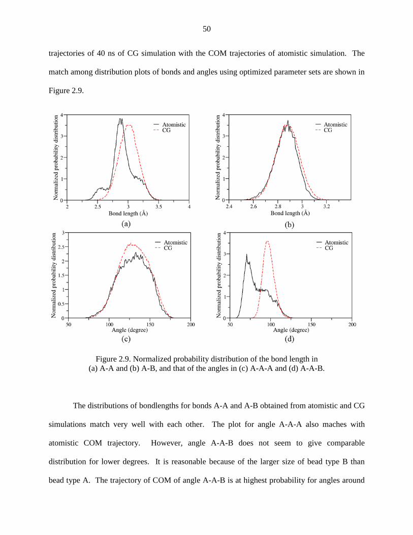
50
trajectories of 40 ns of CG simulation with the COM trajectories of atomistic simulation. The
match among distribution plots of bonds and angles using optimized parameter sets are shown in
Figure 2.9.
Figure 2.9. Normalized probability distribution of the bond length in
(a) A-A and (b) A-B, and that of the angles in (c) A-A-A and (d) A-A-B.
The distributions of bondlengths for bonds A-A and A-B obtained from atomistic and CG
simulations match very well with each other. The plot for angle A-A-A also maches with
atomistic COM trajectory. However, angle A-A-B does not seem to give comparable
distribution for lower degrees. It is reasonable because of the larger size of bead type B than
bead type A. The trajectory of COM of angle A-A-B is at highest probability for angles around
51
70⁰. In a CG model, values lower than 80⁰ for angle A-A-B lead to bead B coming in close
proximity to the backbone chain. Under such proximity, the beads encounter high steric
hindrance from the backbone chain. Thus, it prevents the angle A-A-B to reach smaller values
than 80⁰.
Parameterization of nonbonded interactions. The nonbonded interactions consist of
contribution from Van der Waals forces and electrostatic forces between polymer beads. In the
CG model of PMMA, both bead types are assigned with neutral charges. Thus, there are no
electrostatic interacations among the polymer chains. According to the MARTINI protocol, the
nonbonded interaction potentials among the neutral beads are represented by LJ function. The
optimization of LJ potential parameters is based on the reproduction of selected target
thermodynamic and structural properties. In this work, PMMA melt density and radius of
gyration are set as target properties for optimization of nonbonded parameters. The CG model of
PMMA considers two different types of beads with four-to-one and three-to-one mapping
schemes. The size and mass for four-to-one mapped bead B is straightforward as 4.7 Å and 72
amu respectively. The size and mass of bead A with three-to-one mapping can be chosen as
same or smaller depending upon the performance of the model in terms of target properties. It
was found that the density obtained using smaller size of A was in better agreement (4.06%
error) than the density using same size of A (12.3% error) with that of the density from atomistic
simulation of PMMA melt.
In simulation, when the initial size () and strength of interaction (ε) values from the
original MARTINI force field were used for both the bead types, the density of the system was
1.161 g/cm3, which was significantly higher than that in the atomistic simulation (1.034 g/cm
3),
and the radius of gyration was also 18% larger. A larger radius of gyration indicated attractive

52
forces between backbone beads which were too weak. Thus, the force of attraction was
increased by adjusting the value of ε between A-A to 3.56 kJ/mol and B-B to 3.7 kJ/mol. Using
these new values, the polymer melt density of the CG model at 500 K was found to be 1.076
g/cm3
(with an error of 4.06%), and the radius of gyration of 1.236 nm was also in good
agreement (with an error of 9.4% error) with that predicted by atomistic simulations. The
performance of the CG model of PMMA was slightly better than the MARTINI model
developed for polyethylene oxide (PEO) chains, where the densities of low molecular weight
PEO are reproduced with an error of 6-8% (Lee et al., 2009). The optimized set of LJ
parameters for all nonbonded pairs of beads are listed in Table 2.2, where Rbond and Kbond are the
bond length and force constant at equilibrium, respectively, and 0 and Kangle are the angle and
the force constants at equilibrium, respectively.
2.3.3 CG Model Verification
One of the important features of thermodynamics-based CG model for PMMA is its
ability to retain molecular integrity at different temperatures. The developed CG model is
verified through reproducing accurately the thermodynamic and structural features that are
obtained from the atomistic simulation.
Density. The system characterized by the CG model consisted equal number of polymer
chains as that in the atomistic model. The chains were allowed to equilibriate for 150 ns under
melt condition at 500 K, and then cooled down at the interval of 100 K and equilibriated for 80
ns at each interval boundary under NPT ensemble. The densities were calculated by averaging
over last 40 ns of trajectory. As shown in Table 2.4, the densities (ρ) evaluated by the CG model

53
and that through atomistic simulations have less than 5% of difference over the temperature
range of 200 K to 500 K.
Structure. In general, CG models tend to lose structural features of a molecule at
changing temperatures. Table 2.4 also shows that the radius of the gyration of PMMA chains
(Rgp) seems to match well with that from atomistic simulation over the entire temperature range.
A closer look at the data indicates that at lower temperatures, the density of polymer chains
become larger, which leads to a smaller radius of gyration. Carbone et al. (2008) performed a
comparative study on the transferability of the models that were obtained through coarse-
graining of polystyrene (structure-based) and polyamide (thermodynamics-based). They
demonstrated that the RDF‟s of only polyamide model showed good comparison and thus the
model was transferable at different temperatures. The CG model of PMMA could retain most of
the structural features at all temperatures of simulation. As shown in Figure 2.10, the RDF
curves of PMMA chains at the simulated temperatures are very close to each other. The first
peak is increasing as the temperature is decreased, this is due to the stiffness of polymer chains at
higher density.
Table 2.4. Comparison of the temperature-dependent density and
radius of gyration of PMMA by the atomistic model and the CG model.
T (K) ρ (g/cm
3) Rgp (nm)
CG Atomistic CG Atomistic
500 1.076±0.012 1.034±0.006 1.236±0.031 1.129±0.020
400 1.121±0.015 1.107±0.009 1.224±0.022 1.113±0.012
300 1.162±0.009 1.154±0.005 1.213±0.019 1.10±0.011
200 1.198±0.007 1.191±0.008 1.199±0.023 1.092±0.018
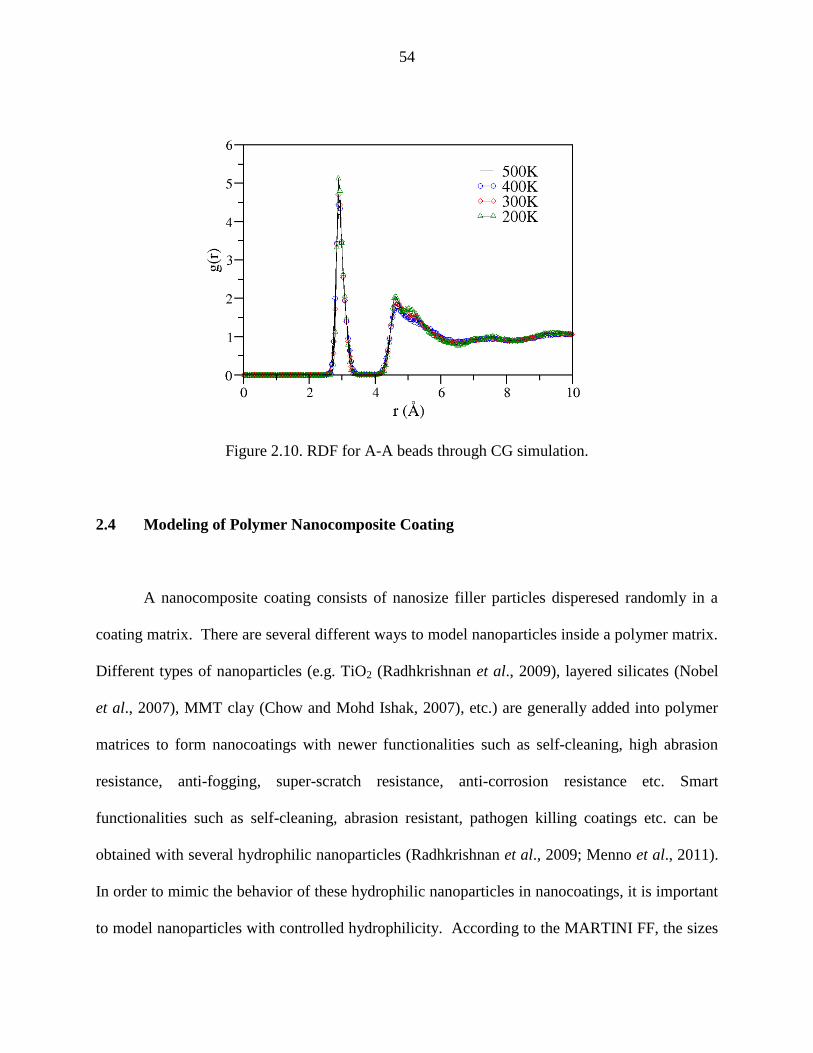
54
Figure 2.10. RDF for A-A beads through CG simulation.
2.4 Modeling of Polymer Nanocomposite Coating
A nanocomposite coating consists of nanosize filler particles disperesed randomly in a
coating matrix. There are several different ways to model nanoparticles inside a polymer matrix.
Different types of nanoparticles (e.g. TiO2 (Radhkrishnan et al., 2009), layered silicates (Nobel
et al., 2007), MMT clay (Chow and Mohd Ishak, 2007), etc.) are generally added into polymer
matrices to form nanocoatings with newer functionalities such as self-cleaning, high abrasion
resistance, anti-fogging, super-scratch resistance, anti-corrosion resistance etc. Smart
functionalities such as self-cleaning, abrasion resistant, pathogen killing coatings etc. can be
obtained with several hydrophilic nanoparticles (Radhkrishnan et al., 2009; Menno et al., 2011).
In order to mimic the behavior of these hydrophilic nanoparticles in nanocoatings, it is important
to model nanoparticles with controlled hydrophilicity. According to the MARTINI FF, the sizes

55
of beads which represent groups of atoms are predefined. These beads are assigned with
different values of ε of LJ interaction potential function. The values of ε represent different
levels of hydrophilicity/hydrophobicity. Marrink et al. (2007) described 9 different interaction
levels with specific values of ε. Higher values of ε can be used to model more attractive
interactions among highly polar groups, whereas smaller values of ε can be used to model
various degrees of hydrophobic repulsions between polar and nonpolar phases.
Studies on atomistic level simulation have shown that C60 fullerenes form spherical
nanoparticles by closed packing large number individual entities to form spherical nanoparticles
(Bedrov et al., 2005). At CG level, nanoparticles are modeled using clusters of small sized beads
to form various shapes of nanoparticles (Knauert et al., 2007). We adopted a similar
methodology to form spherical hydrophilic nanoparticles. The modeling of each nanoparticle
inside the polymer matrix was performed using LJ beads of size 4.7 Å. A cluster of large
number of beads connected to each other was created to form spherical nanoparticles. The
number of beads needed to form these CG nanoparticle clusters were calculated using the
volume of each individual bead and the total volume of each nanoparticle. The interactions
between the beads were defined using only the LJ potential. For this work, the nanoparticle
beads are named as “NP”. They are analogous to the bead type “P1” of MARTINI force field
(hydrophilic beads with lower polarity). The strengths of interactions between nanoparticle
beads and polymer beads are summarised in the table below.
Table 2.5. LJ potential parameters between NP
and polymer beads.
Bead types ζ (Å) ε (kj/mol)
NP-NP 4.7 4.5
NP-A 4.7 2.7
NP-B 4.73 4.5

56
The simulation of nanocomposite coating was performed under NVT ensemble. These
simulations were performed at longer time steps upto 25-30 ns to reach the equilibrium quicker.
Under the melt condition at 500 K and atmospheric pressure, the polymer chains move freely and
avoid getting trapped in one state of configuration. The sizes of nanoparticles and number of
polymer beads decide the system size and thus the cutoff length for LJ potential. A long
simulation time of 300 ns ensured reaching of the equilibration state and generation of sufficient
trajectory length to extract data for measurement of structural properties. Generally, an average
over a trajectory of last 50 ns is used for extracting data for analysis. The behavior of polymer
beads was studied by keeping all the nanoparticles fixed at different locations inside the
simulation box and the polymer was allowed to equilibriate.
The system was constructed using 15 chains of PMMA with 50 repeating units in each.
The total number of polymer beads in the system were 1500. The size of the anoparticle
incorporated into the matrix was 3 nm. Note that the interaction among nanoparticle force sites
is stronger than the interaction between polymer and nanoparticle beads. This stronger
interaction prevents the polymer chains from entering inside the nanoparticle framework. It has
been studied that the interface between the polymer and the nanoparticle plays a critical role in
defining improvement in properties of nanocomposites (Starr et al., 2002; Jankar et al., 2010;
Xiao et al., 2010). We studied the movement of polymer chains in the vicinity of nanoparticle
surface. Figure 2.11 illustrates the behavior of polymer beads around nanoparticle surface at the
end of equilibration process of the initially built system with one nanoparticle surrounding
polymer chains. A “Visual Molecular Dynamics (VMD)” software package was used to
visualize the 3D structure (Humphrey et al., 1996). The grey, green and blue colors represent

57
bead types NP, A and B respectively. As the simulation proceeds the polymer chains move
towards the surface of nanoparticle and assemble into a structured pattern leading to a high
density of beads at the interface. Figure 2.12 represents the number density distribution of
polymer beads at different distances from nanoparticle center before (a) and after (b) the
equilibration step. A peaks generated at the end of equilibration are due to the substantial
increase in the number of polymer beads on the nanoparticle surface. It is the result of a
formation of structured pattern of polymer beads at the interface. This phenomenon was also
observed by Xiao et al. (2010).
Figure 2.11. Structures of nanocomposite: (a) the initial configuration, and
(b) the final configuration after equilibration (where bead types NP,
A and B are colored in grey, green and blue, respectively).
(a) (b)

58
Figure 2.12. Number density distribution of polymer beads at different locations from
the center of NP (3 nm size) (a) before and (b) after equilibration (cont‟d).
Figure 2.12. Number density distribution of polymer beads at different locations from
the center of NP (3 nm size) (a) before and (b) after equilibration.
(a)
(b)
59
2.5 CG Model Analysis and Evaluation of Properties
In order to be able to predict accurate properties and performance features of the coating
system using this methodology, it is important to analyze the model for its accuracy in
reproducing the data from atomistic simulations and also from experiments. The model being
thermodynamically stable, it is also necessary to demonstrate its stability at different
temperatures.
2.5.1 Radial Distribution Function
The analysis of the stability of the model and capacity to reproduce all the polymers
structural features over a wide temperature range was demonstrated using radial distribution
function g(r) of polymer chains. When compared the curves representing the structure at
different temperatures ranging from 200 K to 500 K, the CG model retained most of the
structural features even at lower temperatures. The RDF plots of PMMA chains at different
temperatures given in Figure 2.10 have all the peaks retained at same location. The height of the
first peak is seen to be increasing with the temperature as a result of increasing stiffness of
polymer chains at lower temperatures.
2.5.2 Microstructure Analysis
In this section we investigate various simulations performed on polymer-nanocomposite

60
samples by changing the structural parameters of both. We know that incorporation of
nanoparticles in the polymer matrix causes polymer chains to move towards nanoparticle surface
and orient in a highly dense pattern (Xiao et al., 2010). But there are several factors that resist
the movement of bulk polymer and its microstructure on polymer-nanoparticle interface. By
using MD simulation under NVT ensemble, we analyze the effect of nanoparticle size, polymer
chainlength and polydispersity on the behavior of polymer beads in the vicinity of nanoparticle
surface.
Effect of NP size. It has been proven that an interface between nanoparticle and polymer
plays a key role in achieving superior properties of a nanocomposite coating. Xiao et al. (2010)
demonstrated the formation of a structured pattern by polymer beads at the interface. The
structured assembly of polymer beads causes an increase in the number density distribution.
Consequently, it leads to improvement in the mechanical properties of the coating. The
improvement in mechanical and rheological properties of nanocomposites is a function of
surface area of nanoparticles exposed to polymer chains (Jancar et al., 2010). There are several
different shapes of nanoparticles that are used to introduce different features into coatings.
Nanoparticles could be rod like, spherical, sheet, platelet shaped, etc. Spherical TiO2 and layered
silicate nanoparticles of are amongst the most common ones in coating industries that give
substantial improvement of mechanical, rheological or thermal properties and also sometimes
brings in new functionalities like self-cleaning and anti-corrosion coatings (Zhang et al., 2005;
Chow and Mohd Ishak, 2007; Chen et al., 2008; Radhakrishnan et al., 2009).
In order to model comparable size of nanoparticles, we first model spheres by close-
packing multiple LJ beads into a spherical shape. As an initial case study, we model these type

61
of nanoparticles by assigning hydrophilic LJ parameters to individual beads which form
spherical nanoparticles, as also explained in the “modeling of polymer nanocomposite” section.
Experimentally it has been determined that nanocoating samples with smaller sized NP
show better performance of the final film than the ones with larger sized NP in it (Manoudis et
al., 2007). In this work, the effect of size of spherical NP on the structured pattern formation of
polymer around NP surface is investigated by simulating a single NP disperesed in PMMA. In
each case, a total of 1,500 polymer beads is used. As shown in Figure 2.12, the highest density
of polymer beads is obtained within 6 Å of the NP surface. Figure 2.13 shows that the density of
polymer beads at the polymer-NP interface goes down as the size of the NP is increased.
Figure 2.13. Polymer beads density at 6 Å distance
away from NP surface for increasing NP size.
The average radius of gyration of polymer chains is evaluated and used to analyze the
structural properties. It is observed that incorporation of nanosize fillers can stretch polymer
chains, thus increasing the radius of gyration. It is found that if the incorporated nanofiller is

62
larger in size, the average radius of gyration of polymer chains near the interface becomes larger.
Figure 2.14 shows a linear increase of the ratio of radius of gyration in a nanocomposite relative
to the pure polymer melt as the size of incorporated nanofiller is increased, which, indicates the
stretching of polymer chains. This stretching creates more free volume at the interface, and thus
reduces the polymer bead density.
Figure 2.14. The ratio of the radius of gyration of polymer in presence of
NP to that in absence of NP as a function of the radius of NP.
Effect of nanoparticle volume fraction. In simulation, different concentrations of
dispersed spherical NP are tested to evaluate the impact on nanocomposite performance. As
shown in Table 2.6, the total surface area of NP is kept same (28.26 nm2) in all four cases. Then
the average radius of gyration of polymer chains in each case is measured. The stretching of
polymer chains due to interaction with NP‟s gives rise to a large radius of gyration as compared

63
to a pure polymer case. Analysis of the radius of gyration suggests that the free volume available
for polymer chains to stretch is less when the volume fraction of NP is higher.
Table 2.6. Radius of gyration of polymer chains at
different NP concentrations.
No. of
NP‟s
NP radius
(nm)
Total NP
surface
area (nm2)
Rg (nm)
1 1.5
28.26
1.65±0.15
2 1.06 1.612±0.13
3 0.866 1.633±0.16
4 0.75 1.59±0.19
Effect of polydispersity. It is a known fact that polydispersity of the polymer matrix
under consideration plays a critical role in defining various performance properties of a
nanocomposite. Gilman et al. (2000) studied the flame retardancy of a polymer nanocomposite
having MMT clay platelets dispersed around polystyrene resin. It was determined that the
organically modified PS-MMT grade does not show improvement in flame retardancy over
immiscible PS-NaMMT sample. The organic treatment degrades the polymer thus increasing its
PDI. According to Robello et al. (2004), the PS-clay nanocomposite grade with lower PDI of
polystyrene shows an exfoliation of nanoparticles with very less agglomeration, unlike in the
sample with higher PDI of PS. In this section we study the effect of polydispersity on the
assembly of polymer beads around nanoparticle surface.
We carried out simulations of a nanocoating sample with varying number of polymer
chains of different chain lengths. For the first case study, the chain length was varied from n=40
to n=70. The total number of polymer beads in the system were kept the same for each case.
The size of the nanoparticle was fixed to 3 nm. The simulations were run at NPT ensemble for
300 ns with 30 fs time step. At the end of equilibration the total number of polymer beads at 6 Å
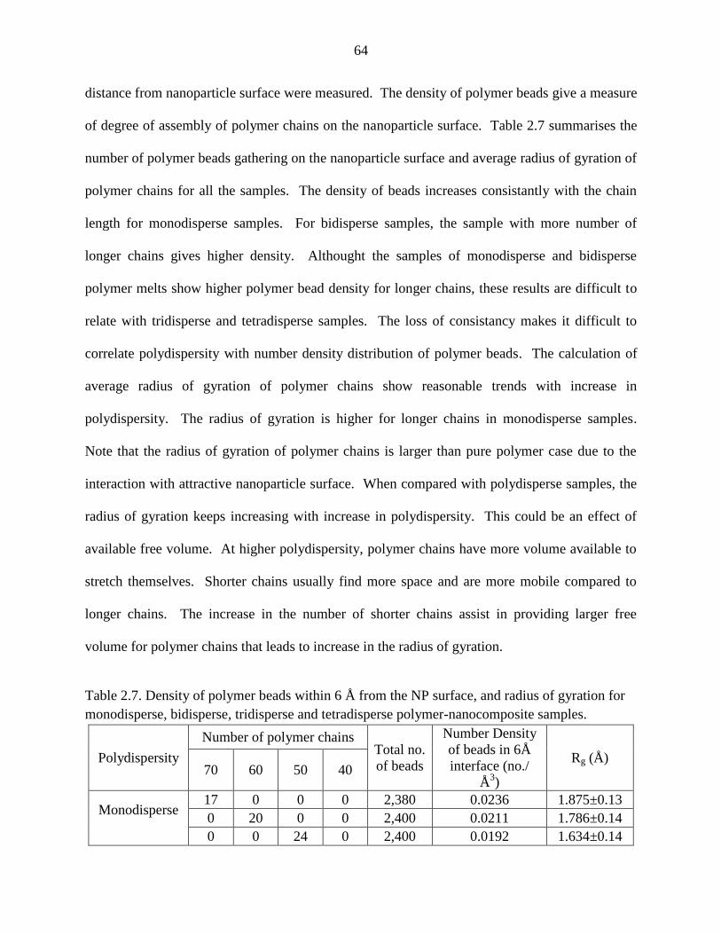
64
distance from nanoparticle surface were measured. The density of polymer beads give a measure
of degree of assembly of polymer chains on the nanoparticle surface. Table 2.7 summarises the
number of polymer beads gathering on the nanoparticle surface and average radius of gyration of
polymer chains for all the samples. The density of beads increases consistantly with the chain
length for monodisperse samples. For bidisperse samples, the sample with more number of
longer chains gives higher density. Althought the samples of monodisperse and bidisperse
polymer melts show higher polymer bead density for longer chains, these results are difficult to
relate with tridisperse and tetradisperse samples. The loss of consistancy makes it difficult to
correlate polydispersity with number density distribution of polymer beads. The calculation of
average radius of gyration of polymer chains show reasonable trends with increase in
polydispersity. The radius of gyration is higher for longer chains in monodisperse samples.
Note that the radius of gyration of polymer chains is larger than pure polymer case due to the
interaction with attractive nanoparticle surface. When compared with polydisperse samples, the
radius of gyration keeps increasing with increase in polydispersity. This could be an effect of
available free volume. At higher polydispersity, polymer chains have more volume available to
stretch themselves. Shorter chains usually find more space and are more mobile compared to
longer chains. The increase in the number of shorter chains assist in providing larger free
volume for polymer chains that leads to increase in the radius of gyration.
Table 2.7. Density of polymer beads within 6 Å from the NP surface, and radius of gyration for
monodisperse, bidisperse, tridisperse and tetradisperse polymer-nanocomposite samples.
Polydispersity
Number of polymer chains Total no.
of beads
Number Density
of beads in 6Å
interface (no./
Å3)
Rg (Å) 70 60 50 40
Monodisperse
17 0 0 0 2,380 0.0236 1.875±0.13
0 20 0 0 2,400 0.0211 1.786±0.14
0 0 24 0 2,400 0.0192 1.634±0.14

65
0 0 0 39 2,400 0.0183 1.489±0.11
Bidisperse 0 15 6 0 2,400 0.0241 2.445±0.22
0 10 12 0 2,400 0.0225 2.631±0.23
Tridisperse 0 8 9 7 2,420 0.0201 2.866±0.15
Tetradisperse 5 5 5 8 2,440 0.0228 3.136±0.21
2.6 Summary
This work provided a detailed analysis of structural and thermodynamic behavior of
polymer chains at the interface of polymer and NP. The modeling and simulation of PMMA
chains surrounding hydrophilic NP cluster was performed using the MARTINI based coarse-
graining methodology. Model verification was provided by reproduction of structural and
thermodynamic properties of the polymer obtained through atomistic simulation that was
performed using an optimized set of CHARMM force field parameters. The predicted densities,
radii of gyration and distributions of bonds and angles were in good agreement with that from
all-atom simulations over the temperature range of 200 K to 500 K.
The deveoped model of polymer-nanocomposite system was applied for the study of
structural behavior of polymer chains around induced nanofillers with varying NP size, volume
fraction and the polydispersity of the polymer PMMA. It is found that the radius of NP‟s
dispersed in nanocoating resin changes polymer bead density and the radius of gyration of
polymer chains. For samples with large NP‟s, the interfacial polymer bead density is smaller and
the radius of gyration is larger than for samples with small NP‟s as a result of availability of
more free volume. It was also shown that increasing the polydispersity index of polymer matrix
elongates polymer chains. These results favor a selection of polymer matrix with low
polydispersity index with more number of longer chains and a higher volume fraction of NP‟s
with smaller size to obtain higher interfacial density of polymer beads.

66
The developed CG parameter set for PMMA and the simulation methodology for
corresponding nanocomposite modeling should be promising as they can be valuable in the study
of water-dispersible acrylic nanocoating systems. Additional nanocoating parameters, such as
self-cleaning, and corrosion resistance, can also be investigated through the developed CG
system.

67
CHAPTER 3
EXPERIMENTAL STUDY ON POLYMER NANOCOMPOSITE COATINGS
From past two decades, polymer nanocomposite coatings are being studied through
various experiments to explore their potential to bring new and significantly improved
functionalities into coating materials. This area of research is still ever increasing through
millions of dollars being invested on it, as innumerable questions related to structure and
material-property correlations of polymer nanocomposites are still unanswered.
The real challenge to this research comes from the limitation of scientific knowledge of
nanocoating microstructure and required methodological-technical development. Needless to
say, that the sustainable nanopaint development is achievable only with an integrated
computational-experimental effort. Such study should be effective in analyzing all the aspects of
the overall life cycle of nanocoating technology, which ranges from nanoparticles synthesis,
through coating formulation, processing, and application to final life-cycle performance. The
experimental analysis of various nanocoating materials and their characterization can not only
provide the verification to the property predictions obtained from computational modeling, but
also it can provide the key insights into the effects of various materials on microstructure-
property correlations.

68
3.1 Objectives and Task Definition
The objective of the research is to develop a comprehensive multiscale methodology to
assist in developing new nanocoating materials with multifunctional performance characteristics
and improved sustainability than conventional coating materials. The outcome from
computational findings would generate critical information about the microstructural behavior
and the correlation between material and the bulk mechanical properties of nanocomposite resin.
The computational study would also provide a variety of information for designing the
experiments, which include the recommendations for selecting polymer matrix and nanoparticle
type, size and shape. These findings would be useful in optimizing formulation parameters for
the development of multifunctional nanocoating materials through experiments. In order to
develop the correlation between paint material and bulk properties, computational work needs to
be integrated with experiments. The verification of the modeling methodology through the case
studies of real polymer nanocomposite coatings can support computational findings significantly.
In this work, the experimental efforts focus towards multiple aspects, such as providing
verification to computational modeling and studying the bulk properties of nanosize polymer
nanocomposite films. The steps followed to achieve these objectives are as follows:
(i) Polymer nanocomposite coating synthesis. TiO2 nanoparticles are photocatalytic in
nature. A nanocoating formulation using selected polymer resin and TiO2
nanoparticles would be synthesized. The nanoparticles would be surface treated to
aid the formation of stable dispersion without aggregation into polymer matrix. The
selection of polymer resin type, solvents and size and shape of nanoparticles decide
the performance of the final coating film.

69
(ii) Analysis of nanocoating formulation. The formulated nanocoating resin will be
analyzed for nanoparticle aggregation or uniform dispersion using SEM (scanning
electron microscopy), AFM (atomic force microscopy) or other high resolution
electron microscopy.
(iii) Application of coating material on panel surface and sample development. Nanosize
coating film would be generated using sophisticated spin coating applicator.
(iv) Coating films‟ analysis for multifunctional performance. The cured nanocomposite
films would be subjected to mechanical testing with nano-scratch indentation for the
film stiffness analysis. Tapping mode AFM imaging would be employed to
determine the nano-scratch depth and paint film morphologies. Self-cleaning
functionality would be quantified through measurement of paint film surface
properties. The measurement of contact angle change would give a degree of super-
hydrophilicity achieved with the TiO2 nanoparticles addition.
(v) Verification of computational models. The formulation recipes and coating films
would be analyzed thoroughly to study the effects of nanosize film thickness and
morphology on the mechanical properties. The film stiffness and mechanical
properties will be compared with the computational modeling results and the
prediction of same properties through molecular simulation will be verified.
Project definition. Nanoparticle induced coating compositions have significant number
of benefits over their conventional counterparts. However, there are several factors related to the
formulation, structure and application of nanocoatings which may affect their improved
performance. These factors include types of polymer resin and nanoparticles, size, shape and
chemistry of nanoparticles, distribution of nanoparticles within cured coating films, nanoparticle

70
aggregation, adhesion of the film to the substrates and with other coating films in multi-coat
applications, rheological properties of nanocoating resins, application techniques, etc.
A thorough research is in progress to correlate nanoparticle morphological parameters
with enhanced performance properties of the final polymer nanocomposite. In case of coatings,
it is believed that the distribution of nanoparticles inside the coating film is a crucial factor which
dictates the mechanical and barrier properties of the final film. It has been shown that the super-
hydrophilicity or self-cleaning feature of coating films can be controlled by applying layer-by-
layer films of TiO2 and SiO2 nanoparticle dispersions of known thicknesses (Wu et al., 2007;
Permpoon et al., 2008). This type of assembly of nanoparticle layers within a coating film can
also change the mechanical properties of the film. A very little attention has been given towards
this correlation between the mechanical properties and nanoparticles distribution inside the cured
coating film. Our objective of the project is to analyze the change in mechanical performance as
a function of location of nanoparticles layer inside the coating film. It is accomplished by
sandwiching TiO2 nanoparticles layer within two PMMA thin films, as shown in Figure 3.1.
Figure 3.1. Coating film structure after sandwiching nanoparticle
film between two polymer thin films.
The current nanocoating films have random distribution of nanoparticles inside the
coating film. We believe that if the distribution is controlled and the nanoparticles are
concentrated at a location which would give maximum enhancement of the final properties, it

71
can lead to nanocomposite coating formulations with significantly improved performance. If this
phenomenon is studied thoroughly and the research predictions are verified, the findings can also
provide directions to the discovery of next generation nanocoatings which would require a single
layer of paint to perform all the functions delivered by current technique of multiple layers of
coatings.
3.2 Materials Selection and Sample Preparation
The polymeric material selected for this study was polymethyl methacrylate (PMMA)
with average molecular weight Mw = 120,000 and glass transition temperature of 105º, purchased
from Sigma-Aldrich. The nanoparticles were anatase-TiO2 type with average particle size <
25nm, purchased from Sigma-Aldrich. The solvent chloroform was used to disperse PMMA.
Silicon wafer substrates of 1 cm x 1 cm dimensions were used for application of nanosize films.
The wafer surface was cleaned using methanol, acetone and water and by immersing the wafer
substrates into freshly prepared pirhana solution for 30 minutes to remove all organic residues
and make a clean hydrophilic surface. A typical pirhana solution is prepared by adding 30%
hydrogen peroxide solution into concentrated sulfuric acid at a ratio of 1:3 (by volume). After
removing from the pirhana, wafers were rinsed thoroughly with deionized water and dried using
air jets.
The bare TiO2 nanoparticles were tested for the solubility in organic solvents. The
selection of appropriate solvent is critical to form a stable and uniform dispersion of
nanoparticles which can be applied on the substrate. The solubility of the bare nanoparticles was
found to be poor in most of the organic solvents. Nakayama and Hayashi (2008) suggested that

72
several efforts have been made to improve the solubility of nanoparticles by surface modifying
these nanoparticles. However, these efforts produced nanoparticles with improved dispersibility
in organic solvents but at a cost of high refractive index of TiO2. The objective of their study
was, (1) to prepare a good dispersion with stability of TiO2 nanoparticles in organic solvents with
surfactants of the minimal quantity, and (2) to disperse TiO2 nanoparticles into the organic
solvents, by exchanging the type of the organic surfactants, without changing the properties of
TiO2 nanoparticles as much as possible. TiO2 has several Lewis acid sites (Ti+) and Bronsted
acid sites (Ti-OH) on the surface. If these sites are capped using both carboxylic acid and amine,
the nanoparticles can form a stable dispersion in organic solvents. The scheme of surface
binding at the TiO2 surface is given in Figure 3.2 (Nakayama and Hayashi, 2008).
Figure 3.2 Scheme of surface binding of TiO2 nanoparticles surface.
The procedure followed for the surface modification of these nanoparticles is as follows
(Nakayama and Hayashi, 2008).

73
1. Bare TiO2 nanopowder was added to excess of propionic acid and stirred for 24
hours.
2. The wet cake was obtained by centrifugation at 5000 rpm.
3. It was washed with ethyl acetate 5 times to remove excess of acid and added into
methanol.
4. The solution of acid modified particles in methanol is mixed with excess amount of n-
hexylamine and stirred for 1 hour.
5. The wet cake obtained by centrifugation at 5000 rpm was washed with ethyl acetate
to obtain the surface modified TiO2 nanopowder.
6. An overnight desiccation drying was done to obtain a dried nanopowder.
The FTIR spectrum of TiO2 nanoparticles was then obtained to ensure the surface
modification. The graph showed absorbence peaks at wavenumbers representing acid and amine
functional groups (See Figure 3.3). These peaks ensured the successful surface modification of
the TiO2 surface. The solubility of the final surface modified TiO2 was also tested in various
organic solvents. The findings are given in Table 3.1.
Table 3.1. Solubility comparison of TiO2 grades in various organic solvents
Solvent IPA Chloroform Methanol
Bare TiO2 Solubility No No Yes
Surface modified TiO2 Solubility No Yes Yes

74
Figure 3.3. FTIR measurement graph for surface modified TiO2 nanoparticles.
A polymer and nanoparticle dispersion films were applied by spin coating technique.
The solutions of PMMA/chloroform were prepared at different concentrations of 0.5, 0.75, 1,
1.25, 2 and 2.5 weight %. All the samples were spun for 60 seconds at rotational speed of 3000
rpm. In order to reduce the surface roughness and to ensure removal of the solvent completely,
the PMMA sample films were kept in an oven at 110º for 30 minutes. TiO2 nanoparticles
dispersion was prepared by dispersing the surface modified nanoparticles into solvent methanol
at a concentration of 0.1 % (by weight). The dispersion was then applied onto the wafer
substrate to form nanoparticle films by spin coating for 60 seconds at 3000 rpm.
For the analysis of elastic moduli of polymer nanocomposite films, three different
samples were prepared using films of PMMA and nanoparticle dispersions as below:

75
(1) PMMA layer of thickness 48 nm using the solution with concentration of 0.75 % (by
weight).
(2) PMMA layer of thickness 48 nm + TiO2 nanoparticles layer using the dispersion of
nanoparticles in methanol
(3) PMMA layer of thickness 48 nm + TiO2 nanoparticles layer + PMMA layer of
thickness 20 nm.
3.3 Film Thickness Analysis
The measurement of polymer film thicknesses was done using X-ray reflectivity (XRR)
technique. Previous work by Walsh and Franses (2003) developed a correlation between PMMA
film thicknesses and PMMA/chloroform solution concentrations at given conditions of spin
coating (see Eq. 3.1).
. . - . (3.1)
where is the film thickness in mm, c is the concentration of the solution in weight percent and
is the rotation speed in rpm.
XRR measurement. In the past decade, X-ray reflectivity (XRR) technique has become
an important tool to study the interfacial properties of thin films (Rao et al., 2004). XRR is a
non-destructive, routine technique which is used for estimation of density, thickness and
roughness of thin film structures. In general, it can be used with crystalline, amorphous and
liquid samples. For the film thickness measurement XRR uses electron density fluctuations at
the interface of two surfaces. The measurement of thickness is based on the total external X-ray
reflection from the surface. This technique is especially suitable to study buried film surfaces as

76
X-rays can penetrate deep inside the coating material. This technique is used for layer
thicknesses between 5Å to 400 nm. In this technique, the diffraction peaks are correlated with
the thickness of polymer film.
For PMMA films applied using polymer dispersions of different concentrations, the
samples were kept inside the XRR instrument and reflectivity data was recorded. The recorded
data curve was analyzed and initial film thickness was predicted using FFT (fast Fourier
transform).
The reflectivity of a single layer deposited on the substrate is expressed using an equation
given as:
2
2
21
2
21
0
0
1tik
tik
z
z
err
errR
(3.2)
where r1,2 are the Fresnel reflectivity coefficients of the free surface and the substrate interface
respectively, k0z is the vertical component of the wave vector of the X-ray beam transmitted
through the film and t is the film thickness. The intensity maxima occurs at all points where
e- t = 1.
During the determination of film thickness using XRR method, the roughness of the
surface plays a key role. In reality, thin film surfaces are not perfectly smooth. The presence of
high surface roughness decreases the specular intensity of the curve and gives rise to progressive
damping of Kiessig fringes. Figure 3.4a,b represents the reflectivity data curves for polymer
films applied onto a silicon wafer substrate using 1% and 2.5% (by weight) solutions of PMMA
respectively. It can be observed that the fringes disappeared for the film of 2.5 % solution due to
higher roughness of the surface. The roughness values are measured using tapping mode AFM
and the values are reported in Table 3.2.

77
Table 3.2. Film thickness values for PMMA solutions at different concentrations
Concentration (%) Roughness (nm) Measured thickness (nm) Thickness from Eq.
3.5 (nm)
0.5 1.1 25.58 31.22
0.75 1.4 48.22 53.54
1 1.6 67.48 78.50
1.25 2.1 101.45 105.63
2 3.5 304.37 197.36
2.5 11.6 350.10 265.56
Figure 3.4. XRR plots for polymer film coated with (a) 1% solution of
PMMA and (b) 2.5% solution of PMMA (cont‟d).
(a)

78
Figure 3.4. XRR plots for polymer film coated with (a) 1% solution of
PMMA and (b) 2.5% solution of PMMA.
The film thickness values are plotted against the concentration of the solutions of PMMA
(see Figure 3.5). The values of the film thickness seem to match well with an error of less than
10% for low concentrations of the solution. At high concentration, the measurement technique
does not produce reliable results because of increase in the roughness of the film surface.
(b)
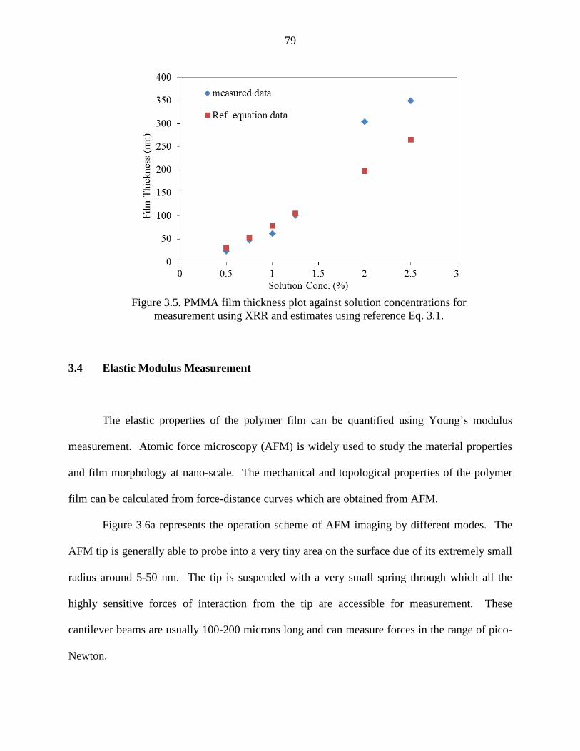
79
Figure 3.5. PMMA film thickness plot against solution concentrations for
measurement using XRR and estimates using reference Eq. 3.1.
3.4 Elastic Modulus Measurement
The elastic properties of the polymer film can be quantified using Young‟s modulus
measurement. Atomic force microscopy (AFM) is widely used to study the material properties
and film morphology at nano-scale. The mechanical and topological properties of the polymer
film can be calculated from force-distance curves which are obtained from AFM.
Figure 3.6a represents the operation scheme of AFM imaging by different modes. The
AFM tip is generally able to probe into a very tiny area on the surface due of its extremely small
radius around 5-50 nm. The tip is suspended with a very small spring through which all the
highly sensitive forces of interaction from the tip are accessible for measurement. These
cantilever beams are usually 100-200 microns long and can measure forces in the range of pico-
Newton.

80
Figure 3.6. Representation of (a) the outline of AFM imaging and (b) force-distance
curve obtained from force calibration mode of AFM.
The AFM is used in the force calibration mode for the measurement of force applied by
the cantilever on the tip. In this mode, the tip is brought together with the surface of the polymer
film in a fluid cell at room temperature. The probe radius is 10 nm and the force constant (k) is
0.06 N/m. The force curves are obtained by bringing the tip in close contact with the surface in
an aqueous medium and recording the force v/s deflection measurements after allowing the
system to equilibrate for 10 min, until reproducible curves are observed. The data of deflection
as a function of piezo position in the z-direction is obtained at different locations on the surface.
The data is analyzed at three different regions of the deflection curve. In the region with
no contact between tip and the surface, the cantilever deflection “d” does not change with respect

81
to the position of piezo in the z-direction. After the contact, the deflection begins to increase
which represents the nonlinear region of the curve.
After the contact the tip indents inside the sample film to a distance δ resulting in small
deflection d = z - . After certain time, the tip reaches the infinite stiffness point where the
deflection curve becomes linear with respect to piezo position and d = z. In generating the graph
for force v/s displacement, the point at which the nonlinear region begins is considered as the
starting point, z0. The data of deflection against z-piezo position is converted into force against
indentation by using Hooke‟s law, where the force F is proportional to the deflection through
cantilever force constant, k.
F = kd = k(z- (3.3)
The final force against indentation curve is obtained by (a) calibrating the sensitivity, (b)
shifting the deflection curve to (0,0) mark, (c) converting the z-piezo movement to indentation
values, and (d) calculating F values using deflection data through Hooke‟s law.
The elastic deformation of the polymer film is represented by Hertzian mechanics
(Mermut et al., 2003). The Young‟s modulus then can be calculated using the equation,
√
-
(3.4)
The Poisson‟s ratio was selected as 0.35 for polymer PMMA film. The radius of the tip
was 10 nm. From the linear plot of log F as a function of log δ, the intercept value was used to
calculate the Young‟s modulus by using the equation below.
l
l +l (
√
- ) (3.5)
Three different samples were prepared for the analysis of elastic properties of the
polymer and nanoparticle layers. The Young‟s moduli were calculated for each of the samples to

82
study the effect of addition of nanoparticles into coating film. The plots of force to indentation
for all the three samples are given in the following figure.
Figure 3.7. Force v/s indentation curves for (a) Sample 1,
(b) Sample 2 and (c) Sample 3.
The surface morphology was studied using AFM imaging under tapping mode. Figure
3.8 shows the AFM images for Sample 3 after coating of each layer followed by curing. It can
be observed that a substantial number of nanoparticles are on the surface after application of the
2nd
layer of nanoparticles. This layer disappears after applying the 3rd
coat of PMMA of 20 nm
thickness. A minimal amount of nanoparticles which are visible in the wet film also disappear
after the sample is kept under heating for 30 min. After heating, all the solvent from the layer
evaporates and the smoothness of the film improves.

83
Figure 3.8. AFM images of surfaces for sample 3 after application of nanoparticle layer (left),
after application of top PMMA layer (middle) and heating of the top layer (right).
The graphs of force as a function of indentation for all three samples were converted into
linear plots by taking a log on each side as shown in Eq. 3.5 and the elastic moduli were
determined. The results are tabulated in Table 3.3.
Table 3.3. The elastic moduli of all three samples of polymer nanocomposites.
Sample Description Elastic Modulus (GPa)
1 PMMA (48nm) 2.25 ± 1.1
2 PMMA (48nm) TiO2 94.15 ± 13.2
3 PMMA (48nm) TiO2 PMMA (20nm) 20.98 ± 10.6
3.5 Summary
In this work, the study of effect of distribution of nanoparticles inside a coating layer on
the film properties was performed. For this study, an acrylic resin (PMMA) which one of the
most common paint resins for water-borne formulations was used along with hydrophilic anatase

84
TiO2 nanoparticles. The selection of water miscible ingredients was done by keeping in mind the
emerging need for low VOC paint formulations.
The polymer and nanocomposite coating layers were analyzed and studied using AFM
technique. The films were applied by spin coating method. The analysis of film thicknesses was
carried out using a sophisticated XRR measurement method. The film thicknesses in the range
of nanosize were obtained using spin coating under controlled operating conditions. The
reliability of the values depends on the roughness of the coating film. The AFM under tapping
mode was employed to determine the roughness values of polymer and nanocomposite coating
films. The force calibration mode of AFM was used to determine the elastic properties of the
films. The calculated elastic modulus for PMMA layer was in good agreement with the
empirical value. It confirmed the applicability of the Hertzian mechanics for the measurement of
elastic moduli of polymer/nanocomposite films. The samples were prepared by sandwiching a
nanoparticles layer in between two PMMA coating layers. The coating layer thicknesses were
controlled such that the final film thickness would remain within the range of 100-200 nm. A
contact mode AFM was applied to perform the mechanical stiffness analysis of each of the
coating layers. From the force to indentation curves, it was clearly seen that the elastic modulus
of the coating film increased significantly after the addition of nanoparticles layer. The results
were in good agreement with the prediction from the computational model which stated that the
evenly distributed nanoparticles inside a coating layer improve the mechanical strength of the
final film.
One of the limitations of this work was the accuracy of the Young‟s moduli values. The
values may not be reliable because of insufficient indentation of the AFM tip inside the coating
film. The reliability of the results can be improved if the indentation atleast reaches the bottom
85
layer (more than 50 nm). It can be achieved with a very strong material, such as diamond, for
the AFM tip.
The future work should focus towards the measurement of accurate Young‟s moduli of
polymer nanocomposite films using hard diamond tips and a stronger cantilever beam of AFM.
The values then can be compared directly with the elastic properties prediction obtained from
computational modeling of the same material. The generation of more nanocomposite samples
by varying the location of nanoparticles film from bottom of the layer to top, followed by
determination of change in mechanical stiffness can generate critical information regarding the
significance of nanoparticles distribution inside a coating layer. If this distribution can be
controlled and optimized for maximum enhancement of the film properties, it can lead to
breakthrough coating technology and a possible single coat application to serve a purpose of
multiple coats (e.g. primer, basecoat, topcoat).

86
CHAPTER 4
MULTISCALE LIFE-CYCLE BASED SUSTAINABILITY ASSESSMENT
(LCSA) OF NANOCOATING TECHNOLOGY
The concept of sustainability deals with the balance in the “triple bottom line”, which is
to accomplish economic development, environmental cleanliness and societal satisfaction
together. Collaborating sustainability approach with life cycle (LC) based study can support the
economic growth of nanotechnology while improving the quality of life and without impairing
public health or detrimental harm to the environment.
4.1 Objective and Significance
The nanocomposite coating material is synthesized by dispersing nanoparticles of
different sizes and chemical nature into polymer resin. The application process of these coatings
consists of spraying the paint on substrates and heating the substrate to allow the film to dry.
The final paint film has numerous applications due to superior performance properties provided
by incorporated nanoparticles. The life cycle of nanoparticle coatings can be divided into
various stages. We define six stages of complete life cycle of nanocoating material, called as
„cradle-to-grave‟ continuum: (1) Raw material selection and preprocessing, (2) Paint
Manufacturing, (3) Paint spray/flash, (4) Curing, (5) End use, (6) Disposal. First four stages
account for nanopaint film development, and remaining two stages account for its use and

87
disposal. Figure 4.1 represents the pathway that connects all the stage of life cycle of a
nanocoating.
Figure 4.1. Life cycle of a nanopaint.
During these several stages, the nanoparticles are very prone release into the surrounding
air and waste water. Assessing the release of nanoparticles and the possible exposure to
environment and mankind is very crucial while framing critical stages of life cycle. These
nanocoatings can be most susceptible to environmental air, water and soil at different stages of
life cycle. TiO2 and SiO2 are most common types of nanoparticles that are added into coating
formulations. Their use in nanocoating systems has been ever increasing due to all the benefits
achievable with them.
The objective of this research is to identify and optimize ways to develop a sustainable
nanocoating system with minimal environmental implications and improved societal safety and
health care while preserving all the economic benefits of this novel technology. To meet this
goal, all the key parameters related to the paint material and properties at each stage of the life
cycle are identified and addressed. The correlations among sets of measurable parameters at
each stage are established. The development of a sustainable nanocoating technology requires a
comprehensive assessment through various appropriate sustainability indicators. The parameter
sets at various stages will guide the development of sustainability matrix selection. The
indicators are able to address the issues related to triple bottom line. The correlations among

88
indicator sets at different stages of life cycle are established. The overall life-cycle based
sustainability assessment from all the stages should guide the development of nanocoating
technology towards more sustainable future products and also highlight the areas of
improvement at each stage of the life-cycle. Figure 4.2 represents a complete framework of the
missions to be accomplished by this study. The developed assessment methodology is
exemplified using case studies of conventional and nanotechnology based coating materials. The
conclusions are drafted and recommendations are made to support the development of
sustainable nanocoating material.
Figure 4.2. Life-cycle-based sustainability assessment structure.

89
4.2 Life Cycle Aspects
The term life-cycle assessment was originally coined and documented in early 1990 in
ISA 14040/14044. This method comprises of four key phases. These key phases and their
correlation is shown in Figure 4.3.
Figure 4.3. LCA framework as defined in ISO 14040/14044.
Life Cycle Assessment is a method for estimating and assessing the resource usage and
environmental impacts attributable to the entire life cycle of a product, from raw material
extraction and acquisition, through energy and material production and manufacturing, to use
and end-of-life treatment and final disposal (ISO 14040, 2006). The impacts consist of ozone
layer depletion, climate change, increase in toxicity of human health and ecosystem, water usage,
etc. The details on the requirements and guidelines for the four phases shown in Figure 4.3 can
be found in ISO 14044 (2006). The goal and scope definition phase provides the details of

90
product system boundaries and functional units. The inventory analysis phase is focused on the
data collection and calculation procedures required to quantify all the measurable entities defined
in phase 1. The life cycle impact assessment aim at aggregating the results from the inventory
analysis and determine product‟s potential for impact on environment and human health. This
process involves connectivity between inventory data analysis phase with corresponding impact
category indicators. The purpose of interpretation phase is to consider all the findings from
inventory data and impact assessment and to provide appropriate conclusions and
recommendations.
In this work, the LCA methodology described above is combined with sustainability
assessment procedure. A comprehensive sustainability assessment of nanocoating technology
considers following phases of the life cycle: (1) paint material selection and preprocessing, (2)
paint manufacturing, (3) paint spray/flash application, (4) curing, (5) end use, and (6) disposal.
The examination of the stages for selection of paint material, manufacturing, processing
and use and its final disposal stages requires careful assessment of energy, resources and impact
on environment through different design and technology alternatives. Although most of the data
required for the assessment is available only from the research papers and industrial practices,
few parameters are very difficult to quantify due to unavailability of appropriate data. Thus, it is
critical to highlight the parameters that can be measured and can be used for the assessment.
These parameters are associated with different time and length scales of measurement. Figures
4.3a through 4.3f shows the framework of parameters selection and their correlations associated
with nanocoating technology at different life-cycle stages. Note that the last stage of disposal
has been ignored as it is least important and would make only a minor impact on the overall
sustainability of the system.

91
For Stage 1 (material selection and preprocessing), seven parameters were identified
which can be quantified either using the material data from industry or the data research papers.
These parameters are as follows:
S1: Paint resin properties (e.g. molecular weight, PDI, functionality, etc.)
S2: Types of additives selected for the paint formulation
S3: Nanoparticles size, shape and orientation
S4: Particle size distribution for pigment
S5: VOC content
S6: Toxicity of each of the formulation ingredient
S7: Raw materials cost
The selection of these parameters was based on the availability of the data for analysis.
More parameters related to energy, water and electricity consumption during each of the raw
material extraction and synthesis could be added. Such parameters were neglected at this stage
due to the limitation of the data.
Stage 2 (paint manufacturing) was assessed using nine different parameter sets which are
given below. The selection of parameters was done such that all the key aspects related to
environmental emissions, social satisfaction and cost for manufacturing and energy consumption
would be considered.
M1: Paint system composition
M2: Concentration of nanoparticles released/exposed to the surrounding during
manufacturing of the paint
M3: VOC emission during manufacturing
M4: Amount of solvent and water consumed

92
M5: CO2 emission and water usage
M6: Quantity of wastes generated
M7: Toxicity index for all the raw materials and ingredients used during the
manufacturing
M8: Amount of energy consumed for all the processes and electricity usage
M9: Recycle factor. It is a measure of quantity of raw materials which can be recycled
The data for these parameters can be easily obtained from a paint manufacturing industry.
The analysis using such data can be very effective in improving the sustainability performance of
the paint manufacturing stage.
For the assessment of Stage 3, the selected parameters can be quantified using the data
from not only paint application industries but also computational modeling. These are as
follows:
A1: Film surface topology parameters
A2: Paint film thickness data
A3: Emission of VOC‟s and nanoparticles during paint application through spray
technique
A4: Wet film defects (e.g. runs, sags, blisters, etc.)
A5: Paint transfer efficiency
A6: Ventilation system performance (e.g. air velocity, energy consumption)
A7: Energy efficiency of the paint-spray system
The data for some of these parameters is very difficult to obtain from the industrial
practices and empirical measurements. Thus, computational modeling and simulation tools can

93
be employed to determine the performance of some of these parameters, especially in case of
nanopaint application.
The paint spray and curing are one of the most energy consuming stages of the life cycle
of coating technology. The quality of the final coating film is also dependent on these stages and
optimization of corresponding operation settings. Thus, it is essential to perform a careful
analysis of these stages in terms of energy, environment and quality. For the paint curing stage
(Stage 4) eight measurable parameters were identified which are enlisted below:
C1: Coating microstructure analysis
C2: Surface roughness after curing
C3: VOC and nanoparticles emission
C4: Film thickness and uniformity (DFT measurement)
C5: Inter-coat adhesion study (film quality parameter)
C6: Over operation settings and parameters
C7: Crosslinking reaction conversion
C8: Net energy consumption by ovens
The 5th
stage (Use/Reuse) is very crucial for social parameters and coating quality
parameters. The performance at this stage is essentially decided by the sustainability
performance of previous stages. The assessment of Stage 5 includes majority of the parameters
related coating quality, performance and toxicity issues. Again, these sets of parameters can be
modified depending upon the type of paint system to be studied. These parameters are enlisted
below.
E1: Gloss retention
E2: Coating film functionalities
94
E3: Cost of the final product
E4: Toxicity and possible hazards on contact with the film
E5: Solvent and water resistance of the film
E6: Scratch resistance and mechanical stiffness
E7: Corrosion inhibition
All the parameter sets enlisted above are general and can be applied for most of the
nanocoating systems. However, these parameter sets can be modified with new type of
parameters if the data is available for a specific type of nanopaint to be studied. The correlations
among these parameter sets over different time and length scales are shown below in Figure 4.4.

95
Figure 4.4. Life cycle of a paint material with measurable parameters and their correlations
at: (a) all stages of life-cycle, (b) paint material selection stage (cont‟d).
(a)
(b)

96
Figure 4.4. Life cycle of a paint material with measurable parameters and their correlations at
(c) paint spray/flash and (d) coating curing stages (cont‟d).
(c)
(d)
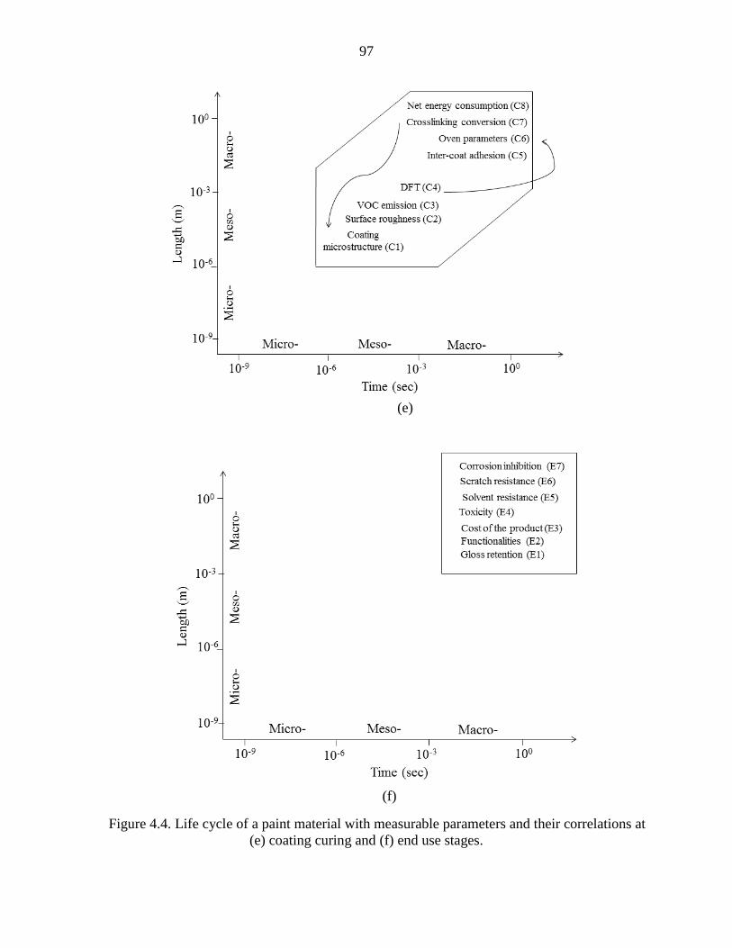
97
Figure 4.4. Life cycle of a paint material with measurable parameters and their correlations at
(e) coating curing and (f) end use stages.
(e)
(f)

98
The quantities of these parameters can be obtained from past research work,
computational models or industrial data. Based on the type of paint material and the available
data, the final choice of parameters can be made which would define the sustainability
assessment framework for the nanocoating system to be examined.
4.3 Sustainability Assessment Framework
In simplest words, “sustainability”, as defined by the 1987 World Commission on
Environment and Development (WCED) as, “Meeting the needs of the present without
compromising the ability of future generations to meet their own needs (Mebratu, 1998)." The
sustainability assessment of nanotechnology deals with multiple dimensions of a design
development and cause-and-effect relationships over various stages of life cycle.
The sustainability assessment is performed using appropriately selected environmental, social
and economic indicator sets. Each indicator is quantified using the reference data for multiple
cases and either absolute or normalized values are obtained. During the life cycle of nanopaint,
each stage is associated with different sets of measurable parameters. Thus, the sustainability
matrix is developed consisting of different indicator sets at each stage of life cycle based on the
set of measurable parameters from that stage (see Table 4.1).

99
Table 4.1. Sustainability matrix over a life cycle of nanopaint.
Stages Economic Environmental Social
Paint Material
selection
Composition of
paint (SI-2)
Material Cost (SI-
6)
Amt. of toxic raw material
(SI-1)
Amt. of solvent/water (SI-3)
Environmental impact factor
(SI-5)
Human health impact
(SI-4)
Paint
Manufacturing
Raw material
composition (MI-
1)
Recycle
efficiency (MI-6)
Net manuf. Cost
and capital
investment (MI-
7)
Release/exposure of
hazardous material (MI-2)
Net solvent/water
consumption (MI-3)
Total energy consumption
(MI-8)
Waste generated (MI-
4)
Toxicity assessment
(MI-5)
Paint spray/flash
Material transfer
efficiency (AI-2)
Net operational
cost (AI-6)
Net VOC/NP emission (AI-
1)
Net energy usage (AI-5)
Film quality
assessment (AI-3)
Human health burden
(AI-4)
Curing
Energy efficiency
(CI-5)
Net operational
cost (CI-6)
Curing process efficiency
(CI-1)
Toxicity assessment (CI-3)
Film quality
assessment (CI-2)
Operational safety (CI-
4)
End use Product cost (EI-
3) Toxicity during use (EI-1)
Coating performance
assessment (EI-2)
Customer satisfaction
factor (EI-4)
Many of these indicators from different stages of the life cycle are correlated with each other.
A change in the value of one indicator from one stage can affect the indicator value at another
stage. Thus, while analyzing the sustainability performance of this technology, a holistic view is
very important. The developed framework pin points some of the important sustainability
indicators which are correlated with each other. In Figure 4.5, these correlations are represented
and the locations of indicators are set at respective time and length scales of measurement.
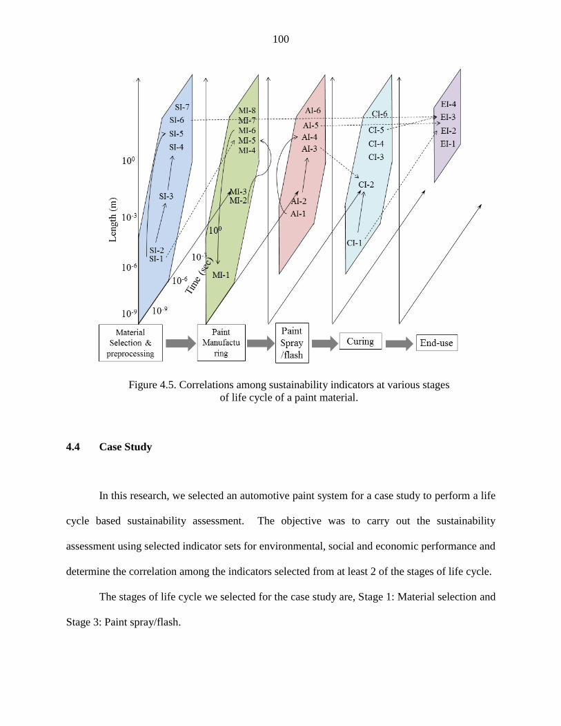
100
Figure 4.5. Correlations among sustainability indicators at various stages
of life cycle of a paint material.
4.4 Case Study
In this research, we selected an automotive paint system for a case study to perform a life
cycle based sustainability assessment. The objective was to carry out the sustainability
assessment using selected indicator sets for environmental, social and economic performance and
determine the correlation among the indicators selected from at least 2 of the stages of life cycle.
The stages of life cycle we selected for the case study are, Stage 1: Material selection and
Stage 3: Paint spray/flash.

101
4.4.1 Stage 1: Material Selection and Preprocessing
This stage of life cycle deals with selection of paint formulation and raw materials
required to manufacture the paint. This is a critical stage which has direct correlation with the
final performance of the coating film. The material selection is based on the required final
properties of the coating film. Several factors related to the toxicity, energy efficiency, safety
and economics of other stages of life-cycle can be improved by improving the sustainability of
this critical stage. In this case we considered the material selection criteria for the determination
of all the indicator parameter values. The preprocessing consists of the information from the
extraction/synthesis of each of the raw materials selected for the formation of paint matrix. Due,
to the unavailability of such data for preprocessing, the indicators related to preprocessing stage
were neglected.
For the case study, we considered two examples of an automotive coating system with 2
coats: basecoat and topcoat. The basecoat for both the examples was a waterborne paint system
while the topcoat in first example was solventborne clearcoat and in second example it was
powder clearcoat. The sustainability assessment of the system with basecoat and topcoat paint
formulations used in the auto industry was carried out by selecting the paint formulations shown
in Table 4.2. The quantities of raw materials given in this table are in weight percent of the total
weight of each of the paint system.

102
Table 4.2. Automotive basecoat and topcoat formulations.
Waterborne basecoat Solventborne clearcoat Powder clearcoat
Material Quantity
(%)
Material Quantity
(%)
Material Quantity (%)
Water 40 Naptha 3 PDMSc 1
Titanium
dioxide
21 Xylene 18 Benzoin 0.5
Naptha 4 Methanol 2 Acrylic/Si
polymer
1
Polyurethane 3 Melamine
formaldehyde
12 Methacrylic
polymer
72
Polyester resin 7 Ethylbenzene 1 DDDAd 22
Melamine
formaldehyde
4 N-butyl alcohol 14
EGMEa 7 Cumene 1
2-
Hexyloxyethanol 2 MTS
b 5
PMMA 10 Butyl acetate 3
PMMA 42
The waterborne basecoat (WB) and solventborne clearcoat (SC) formulations are
commercial products from DuPont and powder clearcoat (PC) is from Seibert which are used for
automotive painting operations (Papasavva et al., 2001). The WB system contains a polyester
and polyurethane resins. Both the resins together form a binder which contributes to 7-14 % (by
weight) of total formulation. The carrying medium is water which accounts for 40-60 % (by
weight). The pigment is white titanium dioxide based (21 % by weight) powder. The average
thickness of the basecoat for the application on automotive body is expected to be 1.0 mil.
The SC system is an acrylic solventborne system. The binder for this system accounts for
54% of the total weight of paint formulation. The expected film thickness to obtain optimum
properties using this coating system is 1.8 mils. The resin for PC system is the glycidyl acrylic
polymer. The resin and crosslinker together contribute to 94% (by weight) of the total
formulation. The optimum film thickness for this system should be 2.2 mils.
aEGME: ethylene glycol
monobutyl ether bMTS: 3-methacryloxypropyl-
trimethoxy-silane cPDMS:
polydimethylcyclosiloxane dDDDA: 1,12-dodecanedioic acid

103
In order to carry out the sustainability assessment we have selected a set of indicators
which address environmental, social and economic aspects of Stage 1 of the life cycle of a paint.
For the paint formulation to be environmentally sustainable it should have a minimum quantity
of raw materials which contribute to VOC. The formulation with higher quantity of water should
be more sustainable. The social indicators are selected to compare the toxicity for human health
and the predicted performance of the final coating. The waterborne basecoat is expected to
provide the color, adherence and hardness to the surface of the automobile, whereas the clearcoat
systems should provide more properties such as appearance, gloss, scratch resistance and
recoatability cost, etc. Economic indicators deal with the composition of each paint and the
material cost. The indicator matrix with relative assessment of both paint formulations is given
in the table below.
Table 4.3. Sustainability indicator matrix for the paint-spray application stage.
Economic Environmental Social
Material Cost Quantity of toxic raw
material (VOC/gal) Predicted performance of
the coating (scale of 10) Composition of paint
(number of ingredients)
Energy consumed per unit
job
For environmental indicators assessment, it can be observed from the formulations that
the system with powder clearcoat should perform better because of zero VOC. In each coating
formulation, it is the polymer resin which consumes maximum amount of energy for the
synthesis. Both the coating systems (WB-SC and WB-PC) are used for coating on an SUV
vehicle. Figure 4.6 shows the amount of energy consumed for the material for each job of
painting an SUV vehicle.

104
Figure 4.6. Comparison of two coating systems for energy consumed per job.
For social sustainability assessment, both the systems performed equally. The predicted
properties of the final film with the selected basecoat and clearcoat systems were similar.
The economic assessment was done by analyzing the material cost and total number of
ingredients required to formulate each type of coating system. The overall sustainability
assessment and comparison between two examples is given in Table 4.4.
Table 4.4. Sustainability assessment matrix for Stage 1 of the life cycle of paint.
Sustainability
Aspect Indicator
Example 1 (WB/SC) Example 2 (WB/PC)
Basecoat Clearcoat Basecoat Clearcoat
Economic
Composition of paint
(no. of ingredients) 9 10 9 5
Material Cost ($/job) 63 40 63 28
Environmental
Quantity of toxic raw
material (VOC/gal) 1.5 4.0 1.5 0.0
Energy consumed per
job (MJ) 467 514 467 406
Social Predicted performance
of the coating 100% 100%
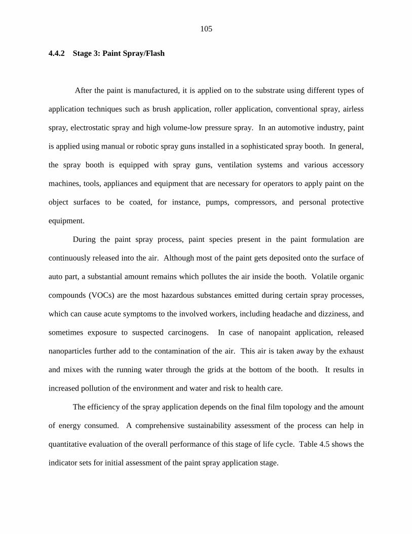
105
4.4.2 Stage 3: Paint Spray/Flash
After the paint is manufactured, it is applied on to the substrate using different types of
application techniques such as brush application, roller application, conventional spray, airless
spray, electrostatic spray and high volume-low pressure spray. In an automotive industry, paint
is applied using manual or robotic spray guns installed in a sophisticated spray booth. In general,
the spray booth is equipped with spray guns, ventilation systems and various accessory
machines, tools, appliances and equipment that are necessary for operators to apply paint on the
object surfaces to be coated, for instance, pumps, compressors, and personal protective
equipment.
During the paint spray process, paint species present in the paint formulation are
continuously released into the air. Although most of the paint gets deposited onto the surface of
auto part, a substantial amount remains which pollutes the air inside the booth. Volatile organic
compounds (VOCs) are the most hazardous substances emitted during certain spray processes,
which can cause acute symptoms to the involved workers, including headache and dizziness, and
sometimes exposure to suspected carcinogens. In case of nanopaint application, released
nanoparticles further add to the contamination of the air. This air is taken away by the exhaust
and mixes with the running water through the grids at the bottom of the booth. It results in
increased pollution of the environment and water and risk to health care.
The efficiency of the spray application depends on the final film topology and the amount
of energy consumed. A comprehensive sustainability assessment of the process can help in
quantitative evaluation of the overall performance of this stage of life cycle. Table 4.5 shows the
indicator sets for initial assessment of the paint spray application stage.

106
Table 4.5. Sustainability indicator matrix for paint-spray application stage.
Economic Environmental Social
Net energy usage Energy efficiency Film quality assessment
Total amount of paint applied Net VOC emission Human health burden
Paint spray booth system. In an automotive industry, paint spray system consists of
several zones through which automotive parts are carried on a conveyor belt. A complete layout
of a typical paint spray system in an automotive plant is given in Figure 4.7. The paint is applied
using compressed air spray guns operated by robotic bells at automatic spraying chambers and
manually by the workers at manual interior cut-in chambers. After each type of paint film
(basecoat and clearcoat) is applied, the parts are carried to the “heated flash off” zone where the
parts are kept under warm ambience to allow uniform film formation and evaporation of
solvents. After flash-off, the coated auto parts are carried to the curing ovens for final film build
and hardening. The curing ovens are adjusted at a very high temperature above the boiling
points of all the solvents and crosslinking reaction temperature in order to allow the film
formation. The lengths of curing zones are adjusted such that the coated parts spend enough
time under high temperatures to ensure high conversion and efficiency of crosslinking reactions.
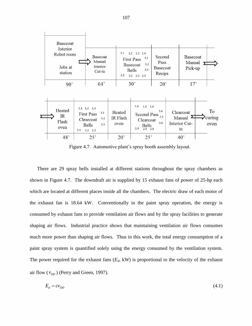
107
Figure 4.7. Automotive plant‟s spray booth assembly layout.
There are 29 spray bells installed at different stations throughout the spray chambers as
shown in Figure 4.7. The downdraft air is supplied by 15 exhaust fans of power of 25-hp each
which are located at different places inside all the chambers. The electric draw of each motor of
the exhaust fan is 18.64 kW. Conventionally in the paint spray operation, the energy is
consumed by exhaust fans to provide ventilation air flows and by the spray facilities to generate
shaping air flows. Industrial practice shows that maintaining ventilation air flows consumes
much more power than shaping air flows. Thus in this work, the total energy consumption of a
paint spray system is quantified solely using the energy consumed by the ventilation system.
The power required for the exhaust fans (Ed, kW) is proportional to the velocity of the exhaust
air flow ( DDv ) (Perry and Green, 1997).
DDd cvE (4.1)

108
where c is a given coefficient (kW/m/s).
Environmental assessment. The environmental assessment was done using the data of
two cases of industrial practices. Both cases assumed the settings for a sports utility SUV car
getting painted in the spray booth. The input parameters and calculated values are given in Table
4.6. The basecoat was water-borne acrylic paint whereas the clearcoat was solvent-borne acrylic
paint. In both the cases, the data related to application of waterborne basecoat onto the car body
was used for the assessment. The VOC concentration of the basecoat paint was 0.4 kg/l. Thus,
the VOC mass flow-rate was calculated as:
Mass flow rate of VOC = TE F. D. VOC concentration (4.2)
where TE is the transfer efficiency (40%) of the paint material and F. D. is a paint fluid delivery.
Table 4.6. Description of industrial cases of paint spray application.
Case No. fluid delivery
(cc/min)
Downdraft
(FPM)
Downdraft
(m/s)
VOC mass flow-
rate*104 (kg/s)
c (energy
coeff.)
kW/m/s
Case 1
(basecoat) 21400 1159 5.88 570 47.48
Case 2
(basecoat) 22100 1160 5.89 589 47.44
The energy efficiency was quantified using the energy coefficient. It gives a measure of
amount of energy that is consumed by the ventilation system.
The net VOC emission was quantified using a relative parameter. The net VOC content
inside the booth is proportional to the quantity of fluid delivered and the downdraft air. We
define this relative term as “VOC factor”, which can be calculated as:
VOC factor = VOC mass flow rate (kg/min) / total downdraft air in FPM (4.3)
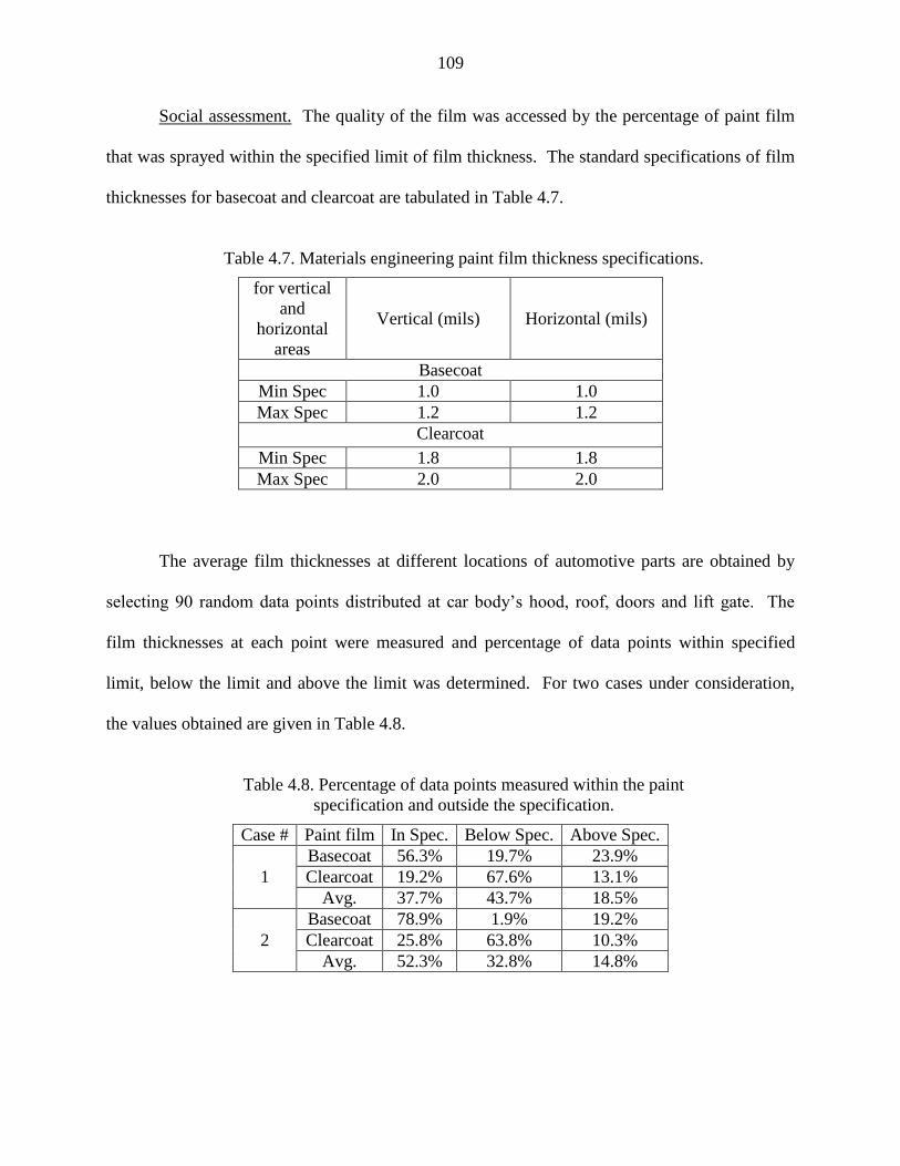
109
Social assessment. The quality of the film was accessed by the percentage of paint film
that was sprayed within the specified limit of film thickness. The standard specifications of film
thicknesses for basecoat and clearcoat are tabulated in Table 4.7.
Table 4.7. Materials engineering paint film thickness specifications.
for vertical
and
horizontal
areas
Vertical (mils) Horizontal (mils)
Basecoat
Min Spec 1.0 1.0
Max Spec 1.2 1.2
Clearcoat
Min Spec 1.8 1.8
Max Spec 2.0 2.0
The average film thicknesses at different locations of automotive parts are obtained by
selecting 90 random data points distributed at car body‟s hood, roof, doors and lift gate. The
film thicknesses at each point were measured and percentage of data points within specified
limit, below the limit and above the limit was determined. For two cases under consideration,
the values obtained are given in Table 4.8.
Table 4.8. Percentage of data points measured within the paint
specification and outside the specification.
Case # Paint film In Spec. Below Spec. Above Spec.
1
Basecoat 56.3% 19.7% 23.9%
Clearcoat 19.2% 67.6% 13.1%
Avg. 37.7% 43.7% 18.5%
2
Basecoat 78.9% 1.9% 19.2%
Clearcoat 25.8% 63.8% 10.3%
Avg. 52.3% 32.8% 14.8%

110
Economic assessment. The operational cost was determined by calculating the total
energy required for running the spray operation. The energy is consumed by the system for
ventilation airflows and shaping airflows. The values of ventilation airflows are recorded in
FPM whereas the shaping airflows are recorded in liter/min. The surface area of the car is 131.8
ft2. The energy (in kW) consumed by the shaping airflows was calculated by the following
formula.
Energy consumed l ate ( - ) .
(4.4)
where (SP-TP) is the static pressure with SP being outlet pressure (inches of water) and TP the
inlet pressure (inches of water) from spray guns. η is the efficiency of the motor associated with
each spray gun. The shaping air flow rate was calculated in CFM. The total energy consumed
by ventilation and shaping airflows for 1 minute of operation in Case 2 (720 kW) is greater than
in Case 1 (691 kW). The cost of each unit of electricity required to generate this energy was
calculated by a two factor utility cost equation which is given as:
CS,u= a (CE PCI) + b (CS,f) (4.5)
where CS,u is the price, a and b are the utility coefficients, CS,f is the fuel price in $/gal and CE
PCI (Chemical engineering plant cost index) is the inflation parameters for all the projects in
U.S. (Ulrich and Vasudevan, 2006). The value of a is 1.3 x 10⁻⁴
and b is 0.010. The inflation
parameter is selected to be in the range of 550 to 600. The fuel price was assumed to be
$3.5/gal. Thus, the unit value of electricity required to generate the energy for case 1 was,
CS,u = 1.3 x 10-4
x 575 + 0.010 x 3.5 = $0.1097/kWh (4.6)
The human health burden was measured as a function of mass flow rate of VOC. The
overall assessment and comparison between two cases is given in Table 4.9. Figure 4.8

111
represents the assessment results in bar-chart, where the “green” colored bars indicate the more
sustainable case and “red” colored bars indicate less sustainable case. It can be observed that
Case 1 is more sustainable compared to Case 2 for four indicators out of selected six selected
indicators.
Table 4.9. Overall sustainability assessment of Stage 3.
Sust. Factor Indicator Case 1 Case 2
Environmental (1) Net VOC emission factor (x10
3) 2.954 3.048
(2) Net energy consumption (kW/m/s) 47.48 47.44
Social (3) Film quality assessment (% In Spec.) 37.7% 52.3%
(4) Human health burden*104 (kg/s) 570 589
Economic (5) Net operational cost ($) 4548 4739
(6) Quantity of paint applied (cc/min) 21400 22100

112
Figure 4.8. Overall comparison of the two cases for the assessment of Stage 3.

113
CHAPTER 5
CFD MODELING OF NANOPAINT APPLICATION SYSTEM – METHODOLOGY
AND SYSTEM DESCRIPTION
In an automotive industry, the topcoat layers are applied on the car bodies by manual or
robotic spray-guns installed inside a spray booth. The paint is applied under optimized
conditions of temperature and humidity. For painting of irregularly shaped objects, manual
spray application is preferred. A typical paint spray technique uses a compressed gas to atomize
the paint material and direct it at a high velocity to the receiving panel through spray guns
(Colbert and Cairncross 2006). Although most of the sprayed paint lands on the target, a certain
amount of paint is carried by the ventilation air and enters the water in the drain through grids on
the booth floor. The effectiveness of paint spray and final coating film quality depends largely
on the operational settings, such as paint flow rate, shaping air velocity and electrostatic voltage
(Li et al. 2007). During paint spray operation, the workers inside the spray booth may become
prone to multiple types of hazards as a result of exposure to VOC, heat overload, electric shock
or electrocution, noise and other types of body injuries. It has been recognized that VOC‟s affect
human health and productivity the most in the manual paint application process due to possible
acute symptoms to workers, including headache, dizziness and exposure to suspected
carcinogens (Feldman et al. 1999; Kim et al. 2000).
For nanopaint, the overspray paint mist is laden with VOC and toxic nanoparticles. It
may severely pollute the booth air as well as the water flowing through the washout. Dunnett

114
(1994) studied how the presence of contaminants and the air flow pattern affect the workers‟
health. If exposed to severe concentrations of toxic nanoparticles such as nanosilica or nano-
titanium dioxide, it can cause fatal health disorders (Reijnders, 2009). Thus, it is important to
develop an optimized paint-spray operation which would be more sustainable in terms of
environmental emission, coating film quality and high transfer efficiency.
5.1 Benefits of CFD Modeling for Paint-Spray System
The study of paint-spray process requires detailed analysis of fluid flow, emission,
atomization parameters and film topology changes. Such analysis is only possible through
computational modeling where individual paint droplets can be tracked and the concentration at
various locations in the spray-booth can be precisely measured. The computational model which
simulates the paint spray application method should also consider the evaporation of solvent
from individual paint droplets during the course of spray. A thorough investigation of the air
quality and energy consumption in the paint spray booth requires an understanding of the
complex fluid flow phenomena in the occupied space of the ventilation air, for which finite
difference-based and Computational Fluid Dynamics (CFD)-based modeling and simulation are
suitable techniques (Tabor et al. 2012).
Li et al. (2013) demonstrated the potential of CFD-based modeling methodology for the
comprehensive analysis of a manual paint-spray system. It was shown that the spray booth
geometry and operation parameters could be adjusted to control the VOC emission below
threshold limit value and to improve the energy efficiency. But, it was assumed that the VOC
was evaporated instantaneously after the paint was injected from the gun. A CFD modeling was
115
also used to characterize the mass transfer and flow of VOC in the booth environment (Flynn and
Sills 2000; Fogliati et al. 2006). It was applied to simulate the breathing-zone concentration for
a paint spray method in a simple spray booth unit with cross-flow ventilation [Flynn, 2000].
Kim et al. (2002) analyzed a small-scale painting process with various exits of air leaving at
different suction velocities. Lu and Howarth (1996) presented numerical results of the prediction
of air velocities, aerosol particle deposition and migration in two interconnected ventilated zones.
Dunnett (1994) presented a study on the effect of the presence of workers on the air flow pattern
and the factors affecting the exposure to contaminants. However, more systematic and
quantitative VOC emission characterization and energy-efficient VOC reduction analysis for
surface coating systems have not been thoroughly studied yet.
5.2 Paint Spray System Design
Since last decade, nanopaints are seen to be replacing conventional paints at several
application areas including automotive, industrial, architectural, military, etc. The induced
nanoparticles of different size, shape and chemical nature provide substantial improvement in
existing product performance and also bring in newer functionalities such as self-cleaning, super-
scratch, anticorrosion, etc. Despite of all the benefits from nano-induced coating materials, it
poses serious concern to environmental safety and health care by unintended release of
nanoparticles into the surrounding medium during manufacturing, application and use phases.
For automotive paint application, the material is applied using conventional, airless or
electrostatic spray techniques. During spraying, the nanoparticles are prone to release in the
surrounding atmosphere and also in the drainage waste water causing serious hazards to

116
atmosphere. Thus, continuous efforts are being made to optimize these spray techniques and
reduce the risk factors associated with the use of nanocoatings.
A typical paint spray technique uses a compressed gas to atomize the paint material and
direct it with high velocity to the receiving panel through spray guns (Colbert and Cairncross,
2006). In automotive sector, the paint spray operation is performed by robotic manipulators.
The paint particles are ejected towards the vehicle body inside the spray booth at a high speed.
Although most of the sprayed paint lands on the target, a certain concentration of paint is carried
by the downdraft air and enters the water in the drain through grids on the booth floor. The
efficiency of paint-spray and the final coating film quality depends on several factors such as
paint flow-rate, paint injection velocity, atomization method, ventilation air velocity, spray angle,
the distance between the gun and the substrate, etc. (Li et al., 2007) The overspray released
during the painting operation is removed by the downdraft air that flows through the booth
geometry and is absorbed by the water flowing underneath the exhaust grid. The removal of the
overspray can be more efficient with higher downdraft velocity of ventilation air. But, it leads to
increased energy consumption. High transfer efficiency can also minimize the overspray
concentration. To improve the process economy and coating film quality, high transfer
efficiency is critical. While spraying nanopaint, the exposure to nanoparticles via different
pathways such inhalation or dermal can cause severe health hazards (Klaine et al., 2008). TiO2,
SiO2, MMT clay, Al, etc. are among the most commonly used nanoparticles in coating
formulations. Research has shown that exposure to high concentrations of such material may
result into possible acute symptoms to workers, including headache, dizziness and exposure to
suspected carcinogens and sometimes can also affect central nervous system (Feldman et al.,
1999; Kim et al., 2000).

117
A paint spray unit includes a spray booth, spray guns/bells, ventilation system, tools,
appliances and equipment such as pump, compressor, conveyor belt and personal protective
gears which are necessary for an operator to apply paint on the object surface to be coated. Paint
material is sprayed using spray bells rotating at high speed. A typical automotive paint spray
application unit is shown in Figure 5.1.
Figure 5.1. Typical automotive paint spray application unit.
The air inside the bells atomizes the paint material and breaks it into tiny paint particles.
For nanopaint, the particles are filled with individual or agglomerated nanoparticles inside it.
The paint particles having nanoparticles are then ejected from the bells at high speed to form a
film on automotive panels. The transfer efficiency of water-borne paint material is generally
around 30-40 % while that of solvent-borne is 60-80%. The remaining paint material is emitted
into the surrounding atmosphere resulting in contamination of the air inside the spray booth.

118
This contamination includes high concentrations of nanoparticles and VOCs. A sophisticated
ventilation system is used to remove the air contaminated with these paint particles.
As described before, the painting of irregularly shaped objects is performed inside a
manual paint-spray booth. As described by Li et al. (2013), a manual paint-spray facility
consists of an air ventilation unit, spray-gun and a placement of substrate to be coated. Figure
5.2 shows a typical manual spray-booth design.
Figure 5.2. Sketch of manual paint-spray booth.
The design consists of a paint spray booth with operational parameters adopted from a
real industrial practice. According to Lin et al. (2005), the spray booth is applicable to chemical
agent resistant coatings, production paints and camouflage and powder paints application.
119
The size of the booth is 19 ft by 39 ft, which is housed in a room of dimensions
approximately equal to 350 ft long and 60 ft wide. Inside the booth, a conveyor belt is located
for moving parts through the working area. Paint is applied by a compressed air-forced paint
gun operated by a worker positioned next to the substrate panel. Generally, an epoxy primer coat
is first applied by spraying, followed by a topcoat films. After painting, the parts are carried out
of the booth into dryers for flash-off and curing. At room temperature, the primer coat dries to
touch in 15~45 minutes and the topcoat dries to touch in 15 minutes. The appropriate paint
thickness of 1.0~1.5 mils for the primer and 1.8 mils for the topcoat is achieved. A successful
paint application job should produce a smooth, continuous, adherent paint film free of runs, sags,
blisters, orange peel, streaks, craters, blotches, fish eyes and pinholes.
The roof of the paint booth is open and air is drawn through a 13 ft wide opening down to
both exhaust air intakes with 4 ft wide slots located on each side of the booth floor. Four 25-
horsepower motors power the exhaust fans to discharge paint fumes outdoor, which give the
exhaust air flows at 80,000 CFM (Cubic Feet per Minute). During the painting operation, fresh
air enters the booth from the open roof and flows down to the floor continuously (see Figure
5.2). Both ends of the booth are kept open. The heating and ventilation facility operates
continuously at all times.
5.3 Integrated Modeling Methodology
The transport of ventilation air, shaping air, injected paint material, VOC and
nanoparticles can be thoroughly examined through CFD-based simulation. Figure 5.3 represents
a general scheme of the modeling methodology and different types of models that are used for

120
the calculation of energy efficiency, VOC emission and nanoparticles emission during the spray
process. This methodology consists of five different models which are described below. Four of
the models were used by Li et al. (2013) for the analysis of VOC emission and energy efficiency
of a paint booth for conventional paint spray. In this work, the discrete phase model was
combined with the previous model to make it suitable for the analysis of nanoparticles-based
paint systems.
Figure 5.3. CFD-based integrated modeling methodology.
5.3.1 Air Flow Model
The air flow pattern within the spray booth is determined by the geometry of the booth
and ventilation system‟s design and setting. It can be characterized by the following dynamic
models, based on the mass conservation principle (see Eq. (5.1)), the momentum conservation

121
principle (see Eq‟s. (5.2)-(5.4)), as well as the realizable k- turbulence principle (see Eq‟s. (5.5)
and (5.6)) (Colbert and Cairncross 2006; Ellwood and Braslaw 1998; Shah et al. 2006). The air
is a continuous phase in the simulation. The prediction of flow of continuous phase is obtained
through a realization k-ɛ model. It is an improved turbulence model as compared to the previous
standard k-ɛ model (Boulet et al., 2010). The governing equations for these models are given
below.
maa Svρρt
(5.1)
i
iaaa Sgρτpvvρvρt
(5.2)
where
Ivμμ3
2vvμμτ ta
T
ta (5.3)
ε
kCρμ
2
μat (5.4)
and
t(
a ) - .(
a ) + . *(μ
a+
μt
) ++ + -
a - (5.5)
t(
a ) - .(
a ) + . *(μ
a+
μt
) + +
+ a
- a
+√ (5.6)
where aρ is the air density (kg/m3), v is the velocity of air (m/s), mS is the rate of mass addition
into the gas phase per unit volume from the dispersed second phase (kg/m3s), p is the pressure
(Pa), τ is the stress tensor of the air (Pa), g is the acceleration due to gravity (m/s2), iS is the
external force on gas phase per unit volume from the i-th species particle (N/m3), a and t
are, respectively, the shear viscosity (Ns/m2) and turbulent viscosity (Ns/m
2), I is the unit

122
tensor, C , 1C , 2C , 3C , and k are the model constants, k is the kinetic energy of
turbulence (m2/s
2), is the dissipation rate of turbulence (m
2/s
3), kG is the generation of
turbulent kinetic energy due to the mean velocity gradient (kg/ms3), bG is the generation of
turbulent kinetic energy due to buoyancy (kg/ms3), and MY is the contribution of the fluctuating
dilatation in compressible turbulence to the overall dissipation rate (kg/ms3). More details about
the realizable k-ɛ model can be found in the ANSYS FLUENT theory guide (2009).
The air within the spray booth is initially static. The fresh air then begins to blow from
booth intake to the exhaust. It is interfered by the shaping air flow near the spray guns. The air
flows out of the booth to the environment through exhaust grids located on the floor. These
operating conditions inside the spray booth are defined by the following initial and boundary
settings of the air flow model.
0boothspraythein0
0exhauststheexceptboundariesphysicalotherat0
0intakesboothat
0guns,sprayofoutlettheat
t,
t,
t,ν
tν
tx,νDD
SG
(5.7)
where SGν is the air velocity from the spray gun (m/s), and DDν is the air velocity of the
downdraft (m/s).
5.3.2 Species Transport Model
Paint species are ejected from the spray guns with a momentum that is governed by two
types of forces: the drag force from the surrounding turbulent air flow and the gravitational force.

123
The velocity of paint species (u) can be modeled by the Newton‟s second law of motion as
shown in the following equations (Colbert and Cairncross 2006; Im et al. 2004).
gftutvm
Dπμ3
dt
tud pa (5.8)
where
ppDm 3
6
1 (5.9)
5
32
1030001 01830
00016
1
rr
r
/
r
Re,,Re.
,Re,Re
f (5.10)
a
apr
tutvDRe
(5.11)
where u (m/s) is the velocity of the species having particle diameter pD (m) and the mass m
(kg), v (m/s) is the velocity of air surrounding the species, f is the drag factor, p is the paint
density (kg/m3) and rRe is the Reynolds number.
The initial species velocity from the spray guns for this model is u0:
0u0u (5.12)
The species trajectory txtr is determined from the species velocity that is determined
by Eq‟s. (5.8) – (5.12). The initial position of all paint species is assumed to be at the outlet of
the spray gun. The dynamic model becomes:
tudt
td tr x
(5.13)
0x0xtr (5.14)
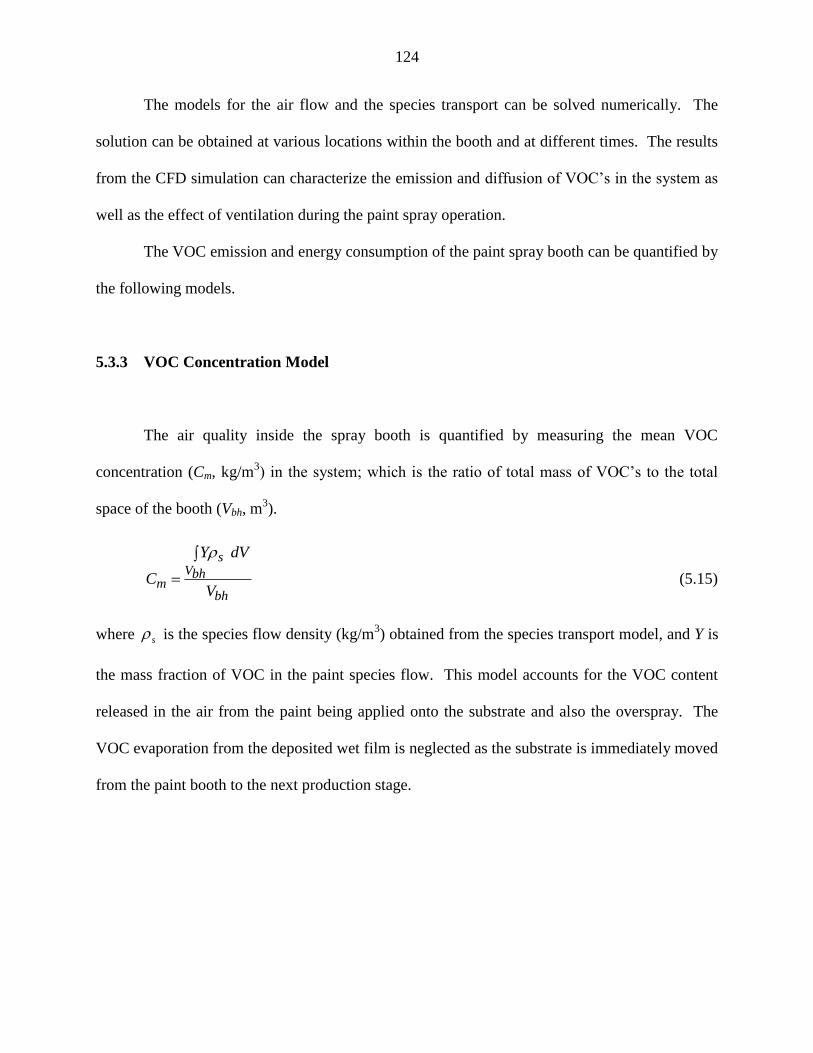
124
The models for the air flow and the species transport can be solved numerically. The
solution can be obtained at various locations within the booth and at different times. The results
from the CFD simulation can characterize the emission and diffusion of VOC‟s in the system as
well as the effect of ventilation during the paint spray operation.
The VOC emission and energy consumption of the paint spray booth can be quantified by
the following models.
5.3.3 VOC Concentration Model
The air quality inside the spray booth is quantified by measuring the mean VOC
concentration (Cm, kg/m3) in the system; which is the ratio of total mass of VOC‟s to the total
space of the booth (Vbh, m3).
bh
bhVs
mV
dVY
C
(5.15)
where s is the species flow density (kg/m3) obtained from the species transport model, and Y is
the mass fraction of VOC in the paint species flow. This model accounts for the VOC content
released in the air from the paint being applied onto the substrate and also the overspray. The
VOC evaporation from the deposited wet film is neglected as the substrate is immediately moved
from the paint booth to the next production stage.
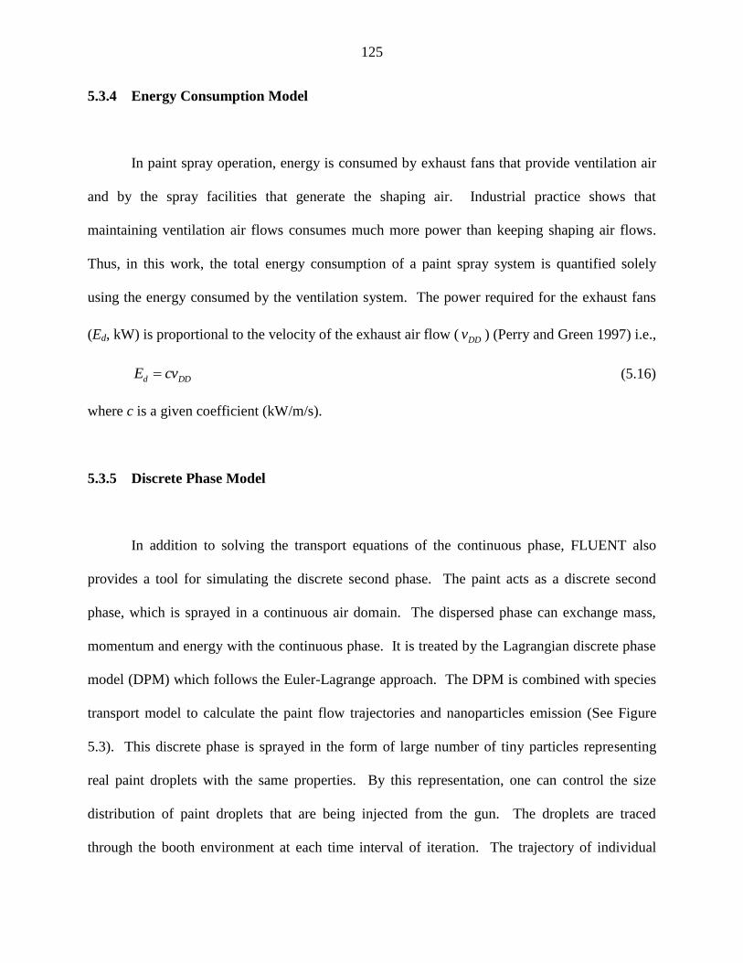
125
5.3.4 Energy Consumption Model
In paint spray operation, energy is consumed by exhaust fans that provide ventilation air
and by the spray facilities that generate the shaping air. Industrial practice shows that
maintaining ventilation air flows consumes much more power than keeping shaping air flows.
Thus, in this work, the total energy consumption of a paint spray system is quantified solely
using the energy consumed by the ventilation system. The power required for the exhaust fans
(Ed, kW) is proportional to the velocity of the exhaust air flow ( DDv ) (Perry and Green 1997) i.e.,
DDd cvE (5.16)
where c is a given coefficient (kW/m/s).
5.3.5 Discrete Phase Model
In addition to solving the transport equations of the continuous phase, FLUENT also
provides a tool for simulating the discrete second phase. The paint acts as a discrete second
phase, which is sprayed in a continuous air domain. The dispersed phase can exchange mass,
momentum and energy with the continuous phase. It is treated by the Lagrangian discrete phase
model (DPM) which follows the Euler-Lagrange approach. The DPM is combined with species
transport model to calculate the paint flow trajectories and nanoparticles emission (See Figure
5.3). This discrete phase is sprayed in the form of large number of tiny particles representing
real paint droplets with the same properties. By this representation, one can control the size
distribution of paint droplets that are being injected from the gun. The droplets are traced
through the booth environment at each time interval of iteration. The trajectory of individual

126
droplet is determined by solving the equation of motion for each droplet. This equation of
motion is obtained from the particle force balance written in a Lagrangian frame of reference
(See Eq. 5.17). This equation considers the forces in the ith
direction of cartesian coordinates due
to drag, gravity and pressure gradient. The thermophoretic and Brownian motion forces are
neglected.
t
+
(
- )+
t( -
) (5.17)
μ
e| - |
(5.18)
e |
- |
μ (5.19)
where is the drag force per unit particle mass, and
are the velocities of fluid phase and
particles respectively, and are the densities of the fluid phase and particles respectively,
is the drag coefficient, is the particle/droplet diameter, is the viscosity of the discrete phase,
is the acceleration due to gravity, and is the Reynolds number.
During the spray of stable nanopaint material, the nanoparticles are not released in the
natural form, but they are surrounded with resin material. Essentially, the overspray paint mist
carries the nanoparticles in the booth environment. The emission of nanoparticles thus depends
upon the paint droplet size and the concentration of the overspray. The simulation of such
mixture of species is accomplished by activating the FLUENT multicomponent particle law (law
7). It allows FLUENT to model each droplet consisting of multiple components with different
masses and densities. The injected particles are allowed to collide or break on interaction with
each other in the air and on the deposited film. The mass of each paint droplet changes
depending upon the evaporation of solvent and collision and break-up phenomena. Droplet
spreading on the substrate film depends on multiple factors, such as, droplet size, injection speed,
127
angle of impact, paint surface tension, viscosity and surface properties such as surface energy,
surface roughness, porosity, etc. The amount of deposition and spreading is determined by the
driving and resisting forces. The driving force is provided by the kinetic energy of the droplet,
whereas resistive force is provided by viscosity and surface tension of the paint material. When
the droplet impacts the surface, its initial spherical shape may change into oval-like form. In
FLUENT, the variation in the droplet shape is accounted by the “dynamic drag model”. The
distortion of shape significantly affects the drag coefficient of the droplet and the value changes
significantly from the drag coefficient of the spherical droplet. The dynamic drag model
calculates the drag coefficient depending on the extent of distortion as given by Eq. 5.20.
)y.(CC sphere,DD 63221
(5.20)
where y is the extent of droplet distortion from spherical to the maximum of disc like shape. In
the case of zero distortion (y = 0), the drag coefficient of a sphere is used, while the maximum
distortion (y = 1) produces the drag coefficient of a disc shape.
5.4 Theory for Paint Spray Atomization and Modeling
A spray is a system of droplets immersed in a continuous gaseous phase. Sprays can be
produced in a variety of ways. Most of the spray application devices achieve atomization of bulk
liquid by creating a high velocity between the liquid and the injected gas required to atomize the
liquid. In order to atomize the bulk liquid into tiny droplets, energy needs to be supplied to the
system. This energy can be provided to the liquid material by employing either high pressure, or
kinetic acceleration. Flowing air bubbles bursting at the liquid surface lead to its conversion into
small droplets which are then sprayed out of the nozzle of the spray applicator.

128
The important properties for the process of atomization of any liquid are density, surface
tension and viscosity. The atomization of the liquid forming tiny droplets occurs when the stable
liquid with certain surface tension and viscosity is influenced by the disruptions from many
internal and external forces. When the disruptive force barely exceeds the surface tension of the
liquid, it leads to atomization and formation of droplets. Most of the bigger droplets are unstable
during the initial breakup of the liquid sheet and form smaller droplets by undergoing further
disintegration. Thus, the characteristics of a liquid spray are governed by the droplet sizes
produced during primary atomization as well as by the extent to which these droplets are later
disintegrated into smaller ones during secondary atomization.
The diameter of droplets which are formed from the flowing liquid through a thin circular
outlet of the spray gun nozzle can be calculated from the following equation (Lefebvre, 1989).
d (6d0ζ
ρLg)
1
3
(5.21)
where do is the outlet diameter, ζ is the liquid surface tension, ρL is the liquid density and is the
gravity constant. The effect of the aerodynamic drag force on break-up of droplets can be
summarized using a Weber number as shown in following equation.
We ρairU
2d
ζ (5.22)
where ρair is the gas density, U the relative velocity and d the droplet diameter.
In spray coating system, the liquid paint is atomized at the nozzle by pressure or
ultrasounds and then it is directed towards the panel by a flowing gas. The tiny droplets that are
formed after atomization land on the surface producing either a full wet layer, in the case of large
paint-flow rate, or sparse depositions and arrangements of dots on the surface, in the case of
smaller flow rates. This droplet spreading in spray coating application is influenced by various
129
factors such as, droplet sizes, impact velocity, impact angle, liquid surface tension, liquid
rheology and substrate surface properties such as surface energy, surface roughness and porosity.
When a droplet hits the surface, its initial spherical shape is forcefully converted into a
pancake like shape. The spreading of paint droplets is decided by the balance of driving and
resisting forces between the droplets and the surface. The driving force is provided by the
kinetic energy of the droplet, whereas resisting force is provided by the surface tension and
viscosity of the paint material. The relative values of the surface and kinetic energies can be
represented with Weber number. For large values of the Weber number the kinetic energy
overcomes the surface tension of the paint and spreading occurs. Whereas, for low values of
Weber number, (e.g. low impact velocity,) the droplets tend to stay spherical and minimal
wetting of the surface takes place.
Droplets are generated by high pressure of the gas during an atomization process. The
injection velocity from the nozzle can be of the order of 100 m/s. However, a reduced velocity is
used for spray nozzles with larger cross sectional area. But, such adjustment is not
recommended as the surrounding air from ventilation may affect the jet velocity and slow down
the droplets flowing towards the surface. Typical droplet sizes for paint material injection
through spray guns are given in the literature which fall between 20-80μm (Toivakka, 2003).
5.4.1 Concept of Particles and Parcels
During DPM simulation, the spray module tracks the discrete phase movement
throughout the system domain. In our case, the discrete phase is paint material. This discrete
phase is allowed to exchange energy, mass (evaporation) and momentum (drag) with the air
130
(continuous phase). In case of spray application, the injected paint material is converted into
millions of tiny droplets which flow through the simulation domain. During unsteady DPM
modeling, the tracking of each of the millions of individual droplets is extremely expensive in
terms of computational efficiency. Thus, in order to improve computational efficiency,
FLUENT code in fact tracks “parcels” and not particles/droplets.
Each parcel is a representative entity of the behavior of many identical droplets after they
are sprayed from the gun. The behavior of the parcels is determined by the behavior of
individual particles. The total numbers of parcels that are generated are determined by various
factors, such as, total mass flow rate, number of particles, particle size distribution, number of
holes on the nozzle tip, and other spray injection inputs.
In general, the number of parcels is calculated by the following equation (Eq. 5.23).
a el t a e (5.23)
where Ntracks is the number of random locations on the gun through which the paint material is
injected and Nsizes is the number of diameters defined in Rosin-Rammler option for particle size
distribution.
The number of particles in each of the parcels is calculated by Eq. 5.24.
a t le
a el
t
a el
(5.24)
where is the mass flow rate of the paint, t is the time step of injection, is the
particle/droplet material density, is the particle/droplet volume. FLUENT tracks these
parcels carrying different number of particles at all the time during simulation. After each
instant of time iteration, the number of parcels is recalculated. The particles can exchange
among different parcels during the course of simulation.

131
5.4.2 Boundary Conditions
The droplet-substrate interaction is an important aspect responsible for formation of the
paint film on the panel surface. FLUENT provides a “wall-film” boundary condition which can
cause the deposition of the paint on the panel. It allows the fluid droplets to impinge on the
surface and form a thin film. The wall-film considers four key phenomena of interaction
between droplets and sample based on the impact energy and wall temperature: spreading,
sticking, rebound and splashing (Stanton et al. 1998 and O‟Rourke 2000). Eq. 5.25 represents
the impact energy (E) as a function of material parameters and the film thickness.
p
bl
p
p
p
p
p
d,
d
hmin
duE
1
1
0
2
2
(5.25)
where paint density, is the droplet velocity, is the diameter of the droplet, is the
surface tension of the paint material and is the boundary layer thickness. If the wall
temperature is below the boiling temperature of the liquid, sticking, spreading and splashing
occur. The number of splashed droplets is set to the default value of 4.

132
CHAPTER 6
CFD MODELING OF NANOPAINT APPLICATION SYSTEM – ANALYSIS OF
ENVIRONMENTAL EMISSIONS AND COATING QUALITY
The CFD-based integrated modeling and simulation methodology which was described in
Chapter 5 was used to investigate an industrial case of a paint-spray booth. Various geometries
and operational settings were simulated and analyzed for determination of an optimum set of
working parameters for minimal VOC emission and energy consumption. The test cases of
various spray-booth systems and detail analysis can be found in Li et al. (2013). The VOC
emission analysis was performed using species transport model and VOC concentration model.
The analyses of nanoparticles emission, coating film topology, transfer efficiency were
performed by integrating a DPM theory with the models for air flow, species transport and VOC
concentration.
6.1 Spray-booth and Paint Material Details
The paint booth geometry for the base case was adopted from the industrial example (Li
et al., 2013). In automotive industries, nanopaints have major applications in clearcoat
formulations. In this work, the paint material selected for modeling was an epoxy-based
clearcoat resin, product no. D.E.R. 538 (www.dow.com/scripts/litorder.asp?filepath=/296-
00312.pdf). For nanopaint formulation, silicon dioxide nanoparticles of uniform size distribution

133
of 100 nm were dispersed into the coating matrix (Huynh, 2006). The solvent used for all paint
formulations was acetone. Based on the industrial data, the paint flow rate was selected as 150
ml/min (Im et al. 2004). The shaping air flow rate from the spray gun is set to 5 m/s. Such a
high value of shaping air flow avoids the coating spray quality from getting affected by the
downdraft ventilation air. The paint droplets were injected at a high velocity of 20 m/s. For the
simulation and analysis of the paint-spray through DPM, three paint systems were selected as: 1)
nanopaint I (with 10% (by weight) nanoparticles); 2) nanopaint II (with 5% (by weight)
nanoparticles); and 3) conventional paint. The solvent concentration and material parameters of
all three systems are enlisted in Table 6.1.
Table 6.1. Material properties of various paint systems
Parameters Nanopaint I Nanopaint II Conventional Paint
Paint Density 1.286 g/cc 1.286 g/cc 1.23 g/cc
NP type SiO2 with 100 nm particle-size -
NP mass fraction 10 % 5 % 0 %
Viscosity 46 cP 43 cP 40 cP
Paint flow-rate 150 ml/min
Size of Paint droplets 10-100 μm
Solvent (Acetone) concentration (lb/gal) 4
For the ventilation air unit, the booth was provided with four 25-hp fan motors. The flow
rate of the exhaust air generated by the fans was 80,000 CFM. Thus, the exhaust air velocity was
calculated as,
v = 80,000 CFM / (2 4 ft 39 ft) = 256.4 FPM (Feet Per Minute) = 1.30 m/s (6.1)
where (2 4 ft 39 ft) is the intake area for the exhaust air. The specified system information
was used to construct the CFD-based models by employing Eq‟s. (5.1) through (5.16). The

134
spray booth consists of four 25-hp fan motors, and the electrical draw of each motor is 18.64 kW.
Thus, the energy coefficient in Eq. 5.16 is calculated as:
c = 4 18.64 kW / 1.30 m/s = 57.35 kW/m/s (6.2)
The performance of the paint spray system, in terms of air purification by ventilation,
quality of the deposited paint film and transfer efficiency depends on multiple factors such as
ventilation air velocity, shaping air velocity, spray pattern, injection tracks, injection angle,
surface roughness, gun-to-substrate distance of separation, etc. For nanopaint spray, toxic
nanoparticles are released in the atmosphere which must be removed to keep the booth
environment safe for workers. The quality of the film may alter due to the addition of
nanoparticles in the paint matrix. The prediction of the coating film topology provides key
information about the role of nanoparticles. For the process to be economical, transfer efficiency
of the paint is a crucial factor. All the parameters are a function of the method of spraying and
operational settings. The optimum performance can be obtained by adjusting the operational
parameters appropriately for each type of coating material to be used. This works studies these
crucial operational parameters which can improve the sustainability performance of the paint
spray system for different types of coating materials.
6.2 Case Study Description
In this work, the paint material was applied on the panel surface with three different spray
patterns. The spray patterns are described below as Cases 1 to 3. In each case, the separation
between the gun and the substrate was fixed at 8”. The performance of each of the three paint
systems was analyzed through CFD-based modeling and simulation to compare the film quality,

135
topological properties and emission of VOCs‟ and NPs‟. The spray patterns and resulting
coverage of the sample by the paint material are shown in Figure 6.1.
Case 1: The paint was sprayed in a cone shape at the center of the sample at a
spray angle of 66.02º. The spray angle was adjusted such that no paint
could be released directly in the surrounding (See Figure 6.1 (a)).
Case 2: The paint was sprayed in a cone shape from the center at a spray angle of
71.67º. This spray angle ensured a complete coverage of the panel
surface. However, a certain portion of paint was allowed to release
directly in the surrounding as overspray (See Figure 6.1 (b)).
Case 3: The paint was sprayed at 5 different locations on the panel for 2 seconds at
each at a fixed spray angle of 58º. The location of spray gun was changed
to four corners and the center of the panel (See Figure 6.1 (c)) in order to
improve the surface topology of the deposited film.

136
Figure 6.1. Spray patterns for (a) Case 1, (b) Case 2 and (c) Case 3.
y
x
x
y
y
x
(a)
(b)
(c)

137
In each case, the paint was sprayed for 10 sec. The fluid was injected along fixed 500
droplet streams from the outlet of the gun. It ensured even distribution of the paint material on
the panel surface in each case. The streams injected droplets of different diameters ranging from
10μm to 100μm. The intermediate droplet size distribution was calculated by applying Rosin-
Rammler distribution function with 50μm as the average size (Alderliesten, 2013). The spread
parameter was set equal to 2. The Rosin-Rammler distribution function calculates the droplet
sizes based on Eq. 6.2.
e-( )
(6.2)
where is the mass fraction of the paint material injected in the form of droplets with diameter
d, is the average diameter and n is the spread parameter. The plot of initial size distribution
based on Rosin-Rammler equation is given in Figure 6.2.
Figure 6.2. Initial droplet size distribution based on Rosin-Rammler function.
The CFD model of the paint spray system considered certain assumptions for the analysis
of each case. These assumptions are,

138
1. The nanoparticles were emitted in the atmosphere in the enclosed form inside a paint
resin.
2. All the nanoparticles were spherical with identical size of 100 nm.
3. On collision of paint droplets on the substrate, the droplets showed one of the four
behaviors: splash, spread, stick and rebound. In the case of splashing, each droplet
would break to form 4 tiny fractions of same size and equal mass fractions.
5. The effect of gravitational force which may cause sagging of wet film was neglected.
6. The collision on walls of paint-booth lead to sticking of the paint material.
6.3 Simulation Details
The models described above were implemented using the ANSYS CFD software
FLUENT, Version 14. A fine mesh was generated with 356746 total elements. The mesh
resolution near the gun outlet was higher to accurately predict the flow dynamics and the
interaction between spray particles and the air. The droplets were injected in a conical fashion
from the spray gun. Unsteady particle tracking was applied for DPM particle treatment. The
particles were sprayed at each particle time step of 0.1 second. Droplet collision and droplet
break-up (WAVE) models were activated to simulate the paint flow behavior during the spray.
Stochastic tracking was applied by discrete random walk model. Coupled scheme was
implemented for pressure-velocity coupling. The pressure discretization was performed under
the second order scheme.

139
The air flow model predicted the air flow profile inside the booth, which was generated
as a result of interaction of downdraft air and shaping air. The contour of air flow velocity is
shown in Figure 6.3.
Figure 6.3. Air velocity contour (a) front view, (b) side view.
(b)
(a)
140
6.4 Spray Trajectories Analysis
The paint droplets were injected from the gun nozzle at a high speed of 20 m/s. Due to
such high speed, the continuous phase had minimal effects on the flow and transfer efficiency of
the paint. For the DPM simulations, the boundary condition for the walls of the booth was
selected such that the droplets would stick after the contact. The downdraft air was allowed to
flow from the opening on the roof to the grids mounted at the floor of the booth. The panel
surface was set as “wall-film”. The trajectories were calculated at every 0.1 sec of iteration time
step. In all the cases, the droplets ejected from the gun were either deposited on the panel or
released in the air.
The flow of paint droplets along the spray booth is represented in Figure 6.4. It can be
seen from Figure 6.4a that the particles with highest residence time (red color) are lying on the
wall of the booth. However, the particles with smallest residence time (blue color) are observed
near the panel. Figure 6.4b represents the paint particles in the air at the end of 10 sec of spray
and as a function of VOC content present in them. The coloring shows that the particles which
are further away from the substrate and have spent longer time in the booth have lesser amount
of VOC in them. This is expected due to higher evaporation of solvents at longer residence time.

141
Figure 6.4. DPM droplet tracks at the end of 10 sec of paint spray as a function of (a) residence
time, and (b) VOC mass fraction.

142
6.5 VOC Emission Analysis
During the spray application, the solvent was continuously evaporating from the paint
material. This VOC vapor contributes to the increasing air pollution inside the booth which
could be hazardous to the worker standing inside. Using this CFD simulation for all the cases,
the vaporized VOC concentration distribution was analyzed. Figure 6.5 represents this
concentration of VOC. It can be seen that the vapor concentration is highest near the sample.
This VOC vapor is taken away with the downdraft air through the grids at the bottom. The spray
booth and ventilation system efficiency is determined by its ability to remove this VOC from the
booth ambience and keep the environment clean for working.
The VOC emission was also analyzed more precisely by calculating the solvent
concentration remaining inside 20 randomly selected droplet streams injected initially at a time
zero. Figure 6.6 represents the trend of solvent concentration change in each of the 20 droplet
streams of Case 1 for all three paint samples. It can be observed that the solvent concentration
was exponentially decreasing along the time. This decrease was a result of continuous solvent
evaporation contributing to increasing VOC in the booth. The occasional increase in the solvent
concentration of few droplets could be caused due to coalescence of several droplets together
after depositing on the panel film. Majority of the droplet streams did not reach 10 sec. It could
also be a cause of coalescence of the droplets with others and spreading on the panel film. A
close similarity among all three graphs (Figures 6.6a through 6.6c) suggests that addition of
nanoparticles in the paint matrix did not affect the solvent concentration trends of all the droplet
streams. Thus, nanoparticles had negligible effect on VOC evaporation during the paint spray.

143
Figure 6.5. Concentration of VOC vapor inside the spray booth after 10 sec of spray.
Figure 6.6. Solvent concentration change during the spray operation of Case 1 for (a) Nanopaint
I, (b) Nanopaint II, and (c) Conventional paint (cont‟d).
(a)

144
Figure 6.6. Solvent concentration change during the spray operation of Case 1 for (a) Nanopaint
I, (b) Nanopaint II, and (c) Conventional paint.
(c)
(b)
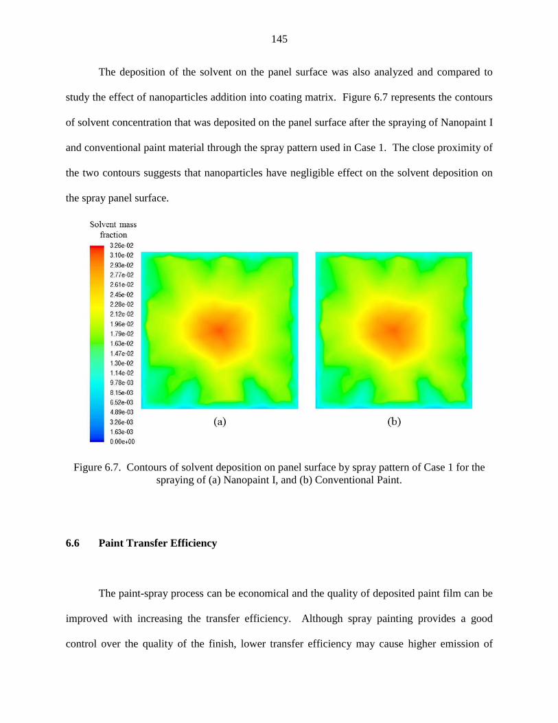
145
The deposition of the solvent on the panel surface was also analyzed and compared to
study the effect of nanoparticles addition into coating matrix. Figure 6.7 represents the contours
of solvent concentration that was deposited on the panel surface after the spraying of Nanopaint I
and conventional paint material through the spray pattern used in Case 1. The close proximity of
the two contours suggests that nanoparticles have negligible effect on the solvent deposition on
the spray panel surface.
Figure 6.7. Contours of solvent deposition on panel surface by spray pattern of Case 1 for the
spraying of (a) Nanopaint I, and (b) Conventional Paint.
6.6 Paint Transfer Efficiency
The paint-spray process can be economical and the quality of deposited paint film can be
improved with increasing the transfer efficiency. Although spray painting provides a good
control over the quality of the finish, lower transfer efficiency may cause higher emission of

146
paint mists. The transfer efficiency of the spray process primarily depends upon the injection
speed and the gun-to-substrate separation distance. The non-transferred paint contributes to the
overspray which causes worker‟s exposure to higher concentrations of paint mist.
The separation distance between gun and sample was fixed to 8” for all the cases
(Beuerle, 1996). The transfer efficiencies of all the cases and types of paints are reported in the
Table 6.2. As expected, Case 1 provided the highest transfer efficiency followed by Case 3 and
Case 2. It can be observed that the nanopaint samples with increasing nanoparticle concentration
have better transfer efficiencies. This could be due to the presence of nanoparticles and increase
in the paint viscosity. The spray of more viscous paint deposited more content on the film and
formed lesser paint mist.
Table 6.2. Analysis of performance parameters for all three cases of paint spray
Parameter Cases Geometry and spray
pattern
Nanopaint
I
Nanopaint
II
Conventio-
nal Paint
Transfer
Efficiency
(%)
1 Spray at the center (partial
coverage of panel) 85.09 81.73 74.93
2 Spray at the center (full
coverage of panel) 74.85 73.86 72.05
3 Spray at 5 locations (full
coverage of panel) 80.91 76.46 72.26
Paint
removed
by the
ventilation
system (%)
1 Spray at the center (partial
coverage of panel) 31.48 31.09 32.02
2 Spray at the center (full
coverage of panel) 30.61 30.71 31.07
3 Spray at 5 locations (full
coverage of panel) 31.12 31.08 32.45
NP‟s
concentrat-
ion in
booth air
(no./m3)
1 Spray at the center (partial
coverage of panel) 1.351x10
12 8.323x10
11 0
2 Spray at the center (full
coverage of panel) 2.307x10
12 1.197x10
12 0
3 Spray at 5 locations (full
coverage of panel) 1.742x10
12 1.074x10
12 0

147
The overspray, consisting of paint solids, nanoparticles and VOC, results in the worker's
exposure to toxic substances. This overspray must be removed efficiently by the downdraft air
in order to keep the booth environment safe for working. For all the simulated cases, the mass
flow and velocity of downdraft air was kept unchanged. The efficiency of the ventilation system
for different cases of paint systems was studied by calculating the proportion of paint removed
by the downdraft air out of total overspray. The corresponding values are reported in the Table
2. It confers that the efficiency of the ventilation system, in case of conventional paint, is
slightly better than that of nanopaint. However, it is preferred to have a high efficiency of
ventilation system, especially in the presence of toxic nanoparticles. Thus, there is a trade-off
between the transfer efficiency and environmental emissions.
6.7 Nanoparticles Emission
The nanoparticles emission during each case was analyzed by calculating the total
concentration of nanoparticles in the booth environment at the end of paint-spray operation. The
values obtained from the analysis are reported in Table 6.2. It can be seen that the higher
nanoparticles content in the paint system invites further risk of nanoparticles emission and
exposure to higher concentrations. Highest concentration of nanoparticles was emitted during
the spray of nanopaint samples through Case 2. With the environmental regulations on NP‟s
emission becoming more strict day-by-bay, it is crucial to have an optimized ventilation system
for nanopaint spray to minimize this exposure which can cause several health concerns.

148
6.8 Film Topology Analysis
The key benefit of paint-spray application method is the ability to control and improve
surface morphology and coating film topology. Spreading of the paint material on the film and
the prediction of velocity profiles of paint droplets are the fundamental factors required for the
accurate determination of surface morphology. Fogliati et al. (2006) determined that the
Realizable k-ɛ model gives most accurate prediction of these characteristics. Thus, the same
model was adopted for the simulation of all the cases.
In order to determine the film thickness profile of the deposited paint layer, the sample
surface was modeled as a “wall-film” which predicts four different phenomena of spread, stick,
rebound and splash of the impacting paint droplets depending on the impact angle and velocity.
The paint mass and deposited film thickness values at various locations on the panel were
recorded. Using these values the plots of distribution of paint thicknesses over the panel surface
were reconstructed and analyzed. The plots obtained for the spray of Nanopaint I using all three
cases of spray patterns are represented in Figure 6.8. The roughness of the film surface was
calculated as the “arithmetic mean roughness ( )” by using the Eq. 10.
ea 1
n ∑ |
|
(6.3)
where is the vertical distance from the mean thickness line to the data point and is the
number of selected ordered and equally spaced data points along the surface of the panel. The
values of the average thickness and roughness of the deposited film from all the cases are
reported in Table 6.3. In order to ensure the reliability of the simulations and the accuracy of the
thickness data, these average thickness values were compared with the theoretically calculated
thickness values. The theoretical thickness is the ratio of quantity of paint that is transferred on

149
the substrate over the cross sectional area of the substrate. The final values were calculated for
each case and the percent error is reported in Table 6.4. For all the cases, the error was less than
8% which verified the reliability of the simulation and the final results.
Table 6.3. Average film thickness and roughness values for all the
cases of all the paint samples
Cases
Average film thickness (μm) Arithmetic mean Roughness (μm)
Nanopaint
I
Nanopaint
II
Conventional
Paint
Nanopaint
I
Nanopaint
II
Conventional
Paint
1 29.70 28.54 25.43 22.26 21.93 18.86
2 25.55 24.55 24.28 14.25 14.11 15.34
3 27.31 26.17 24.30 8.47 8.16 7.79
Table 6.4. Theoretical thickness values and percent error in the calculations
for all the simulation cases
Parameter Cases Geometry and spray
pattern
Nanopaint
1
Nanopaint
2
Conventional
Paint
Transfer
Efficiency
(%)
1 Spray at the center (partial
coverage of panel) 85.09 81.73 74.93
2 Spray at the center (full
coverage of panel) 74.85 73.86 72.05
3 Spray at 5 locations (full
coverage of panel) 80.91 76.46 72.26
Theoretical
Thickness
(μm)
1 Spray at the center (partial
coverage of panel) 29.68 28.50 27.32
2 Spray at the center (full
coverage of panel) 26.11 25.76 26.27
3 Spray at 5 locations (full
coverage of panel) 28.22 26.67 26.35
% error
1 Spray at the center (partial
coverage of panel) 0.08 0.14 3.24
2 Spray at the center (full
coverage of panel) 2.11 4.71 7.58
3 Spray at 5 locations (full
coverage of panel) 4.64 3.36 7.78
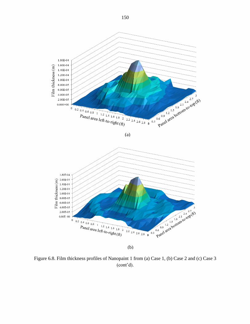
150
Figure 6.8. Film thickness profiles of Nanopaint 1 from (a) Case 1, (b) Case 2 and (c) Case 3
(cont‟d).
(a)
(b)

151
Figure 6.8. Film thickness profiles of Nanopaint 1 from (a) Case 1, (b) Case 2 and
(c) Case 3.
From Figure 6.8, it can be observed that the film topology from Case 3 was substantially
improved as compared to that from Case 1 and Case 2. The thickness values from Table 6.3
suggest that the average thicknesses of nanopaint samples were greater than the conventional
paint. Case 3 showed about 7% improvement of the average film thickness than the worst case.
The roughness was substantially reduced in Case 3 as compared to Case 1. Thus, the spraying of
paint uniformly over the cross-section of the panel showed significant improvement in the film
topology.
(c)
152
CHAPTER 7
CONCLUSIONS AND FUTURE WORK
This chapter concludes the dissertation report with the summary of all the research
findings in the areas of multiscale molecular modeling, life-cycle based sustainability assessment
of nanocoating technology and CFD modeling and simulation of paint application process for the
prediction of nanopaint performance and environmental emissions as compared to existing
conventional paint systems. The summary is followed by recommendations for possible
extension of this work in the future.
7.1 Conclusions
A comprehensive methodology and framework for the multiscale life-cycle-based
sustainability assessment of nanocoating technology has been successfully developed. This
novel technology was studied using computational modeling and experimental analysis on
various levels of time and length ranging from nano- to macro- scales. These modeling
methodologies and corresponding results generated key information required for the
quantification of several sustainability matrixes representing different stages of the life cycle of
nanocoating technology.
The key challenge to the research on sustainability assessment of an emerging technology
such as “nanocoating technology” comes from the limited scientific knowledge and the reliable
153
data availability. Since last decade, nanoparticle-based coating materials are being studied
extensively to determine all the attractive properties achievable with it. It has been proven that
the addition of nanosize fillers of different types and shapes can enhance the polymer composite
as well as coating resin‟s properties tremendously. The final product can have significantly
improved mechanical stiffness, scratch resistance, super-corrosion resistance, antifouling
properties, mar resistance and also certain smart functionalities such as self-cleaning, self-
healing, thermochromic, heat resistance, significantly improved solvent and chemical resistance,
etc. However, it is still unknown how these nanoparticles are responsible for such property
enhancements. The experiments solely are not capable of answering questions and studying the
microstructure-property correlations among nanoparticles and polymer resins. Through this
research, an integrated computation-experimental approach was provided to study these
microstructure-property-performance correlations.
The computational modeling was performed using molecular simulation techniques such
as Monte-Carlo and Molecular Dynamics (MD). In the past, modeling methodology was
developed on macro- to meso- scales of material. This work adopted the bottom-up, deductive
systems engineering approach of materials development. The nanocoating system was simulated
on nano-, micro- and meso- levels and the methodology was connected with the previously
developed system to complete the multiscale modeling methodology of nanocoating system
development.
The nanocoating material was first simulated through MD simulation technique on a
microscale. The microstructural parameters such as bond lengths, bond angles, atomic charges,
dihedrals, etc. were taken from a well-established atomistic force field called “CHARMM”. The
atomistic system consisted of a large number of entities which made the simulation of a
154
nanocoating system with huge design space and complexity computationally very expensive.
Thus, the atomistic design was mapped onto a coarse grained system of “beads”. This was
accomplished by following MARTINI force field development protocols. The bonded and non-
bonded interaction parameters for the system of PMMA-based resin material and TiO2 type
nanoparticles were developed and the system was studied extensively to analyze the structure-
property correlations which cause the enhancement of properties in case of nanoparticles
dispersion. The factors such as, nanoparticles size, volume fraction, polydispersity index, etc.
were studied to determine their effects on final nanocomposite structure. This work was later
coupled with experimental analysis in order to accomplish three key objectives: (a) to provide
validation to the computational modeling work, (b) to study the effect of nanoparticles
distribution inside a coating film on the final mechanical properties, and (c) to lead the
computational-experimental approach towards a new knowledge discovery and optimization of a
“self-cleaning” smart functionality.
It was realized that the optimization of nanocoating formulations solely cannot bring
these emerging products into commercialization due to various types of environmental hazards,
health concerns and economic issues associated with it. Thus, a comprehensive sustainability
assessment framework was developed to look into all the aspects of nanocoating technology, not
only at the manufacturing stage, but over its entire life-cycle which includes all the phases from
material selection and preprocessing, paint manufacturing, paint application and film formation
to its end use and disposal. The developed methodology demonstrated how the sustainability
indicators at various stages of life are correlated with each other. This technology can gain
significant value and the nanoproducts can be commercialized only if its sustainability

155
performance is assessed, compared with existing technologies and further improved to make it a
safer alternative.
However, the challenge to such detailed assessment emerged from the availability of data
for the nanopaint. Thus, Computational Fluid Dynamics (CFD) approach was adopted to
simulate these nanopaints and study the coating quality parameters and environmental emission
factors during application phase. In automotive industries, paint-spray is the most common
application method used for coating the auto bodies. In this research, an industrial paint booth
was designed and the spray of various paint systems was studied. The components which may
primarily affect the environment during paint spray are VOC (Volatile Organic Contents) and
nanoparticles. Through CFD simulation tool, ANSYS FLUENT, the paint spray process was
simulated and the emission of VOC‟s and nanoparticles was thoroughly assessed. This
simulation generated crucial information related to the concentrations of overspray paint and
VOC‟s that was released in the atmosphere and could cause health hazards to the workers inside
the spray booth and pollute the drainage water passing through these paint booths. The final
coating quality parameters were also studied to ensure the superior performance of nanopaints
over conventional paints. The quality parameters such as, film topology, roughness, paint spray
efficiency, etc. were determined and the results for different types of conventional and
nanopaints were compared.
The sustainability assessment framework and multiscale computational modeling
methodologies generated in this research can provide a key pathway towards optimizing an
emerging nanocoating technology and justify the inclusion of nanopaint products into future
commercial market. This research can also assist experimentalists in learning the structure-

156
property correlations of nanocomposite coatings and discover novel formulations of these
materials for the future.
7.2 Future Work
The findings presented in this dissertation provide a solid foundation for the research
related to the development of sustainable nanocoating technology. It can be extended in three
major directions: multiscale molecular modeling of nanocoatings, life-cycle based sustainability
assessment and modeling and simulation of nanopaint application process.
Multiscale molecular modeling of nanocoatings. This dissertation focused on the
development of the multiscale molecular modeling and simulation of nanopaints for the study of
structure-property correlations. The force field parameters and the CG methodology developed
in this research was applied for the study of polymer nanocomposite microstructure. This
sophisticated methodology and the MARTINI force field for PMMA/TiO2 system can be applied
for the study of several other key properties. However, it is important to validate all the model
parameters and the property predictions presented in this dissertation through experiments. The
experimental efforts initiated in this research for the study of polymer nanocomposite films and
determination of properties related to mechanical stiffness and scratch resistance can be further
explored and the validation to the multiscale framework (Figure 1.3) can be provided. The
accomplished work and some of the directions for future work using multiscale MD simulation
method is shown in Figure 7.1.

157
Figure 7.1. Summary of accomplished (non-shaded) and future (shaded) multiscale simulation
work for prediction of nanocoating microstructure-property correlations
With the accomplished work on the multiscale modeling of thermoplastic nanocomposite
coating, the properties such as mechanical stiffness, scratch resistance, barrier properties and
self-cleaning can be predicted. However, a majority of the automotive paint are 2-component,
thermoset systems. The existing methodology can be extended to simulate such thermoset
system by developing appropriate force field parameters for the crosslinker molecules and
verifying them through experiments and empirical data. If succeeded, this model can also
provide validation to the past work which used Monte-Carlo based simulation method to model
generic thermoset nanocomposite coating material.
The CG model for nanocoatings with TiO2 type of nanoparticles can be applied for the
study of “smart” coating materials with self-cleaning functionality. The hydrophilicity of the
nanoparticles play a key role in determining the performance of the eventual nanopaint. This

158
MARTINI force field based CG model can predict the interactions among paint resin and surface
of nanoparticles with different hydrophilicity. This phenomenon can assist in the development
of optimum formulations of nanopaints which can deliver self-cleaning functionality.
The thermoset paint system is a 2K (2 component) system where the 2nd
component is a
cross-linker/curing agent. The curing agent is mixed with the paint vehicle before the mixture is
applied onto car bodies. The cross linking reaction helps in the formation of very hard films
which have significantly better mechanical properties of the film as compared to thermoplastic
paints. The thermosets have been well rooted into automotive paint systems and most of the
existing basecoat and topcoat formulations are thermoset paints. However, the development of
nanoparticles-induced thermoset paints remains a mountain top area of research. The
optimization of thermoset nanopaint formulations is a challenge due to the limited availability of
knowledge about its microstructure. The CG model developed in this research can be further
extended for the study of such systems and the microstructure-property-performance correlations
can be established for thermoset nanopaint materials. Through the MD tool NAMD, it can be
accomplished by developing an optimized CG force field parameters for crosslinker molecule
and then simulate the cured system (as shown in Figure 7.1). However, NAMD does not support
the formation of new chemical bonds and thus the curing reaction to happen during the course of
simulation. This shortcoming of NAMD can be avoided by the use of the MD tool which
supports such reactions. LAMMPS and GROMACS are the best alternate routes which can
perform such reactions during simulation and thus the thermoset nanocoatings can be modeled.
The performance of nanopaints for automotive bodies heavily depends on the size
distribution and shapes of dispersed nanoparticles. The nanoparticles such as TiO2, SiO2,
alumina, MMT clay, etc. have different shapes (e.g. spherical, oval, platelet, crystalline, etc.) and

159
thus they exhibit different characteristics in the final coating material. The multiscale modeling
methodology developed in this dissertation can be applied to study the effects of such shapes of
nanoparticles on the final performance of the coating film.
One of the challenges that the nanopaints are facing for becoming commercialized is
from the issues related to durability. This factor is also related to destabilization of paint due to
aggregation/agglomeration of nanoparticles. This crucial phenomenon can be studied by
modifying the developed PNC system with a system where each nanoparticle is represented by a
single Van der Waal bead. The interaction parameters can be determined by following the same
MARTINI methodology which was applied in this research. Such system can efficiently address
the concerns related to aggregation/agglomeration of different types of nanoparticles in the paint
formulation.
Life-cycle-based sustainability assessment. It has been evidenced by several studies that
the nanoparticles pose serious threat to environment and human health. Needless to say, that the
nanocoating, after commercialization in the future, can also pose such threats to human life and
environment. Thus, this dissertation was focused on the development of a comprehensive life-
cycle based sustainability assessment framework (Figure 4.2) to analyze the performance of
existing nanocoating technology and determine the areas to improve in terms of environmental,
economic and social performance of this technology for making it sustainable. This framework
can be further refined with much extensive research on each of the stages of life cycle by
obtaining more reliable and accurate data for all the sustainability matrix parameters. The
accuracy of the data is the most important aspect which can justify the credibility of this
methodology for the prediction of sustainability performance of different types of nanopaint
systems. The indicator matrixes developed in this work are also generic. More indicators can be

160
explored and this framework can be further improved to make it applicable for a specific
category of nanopaint. For example, the assessment of a nanopaint system which has application
in automotive industry can be more effective if the indicators are more focused towards the
factors such as, durability of the film, energy consumption during application of the films in
paint shops, and final performance of cured coating surfaces.
Another aspect which can be introduced is the “decision-making”. The current LCSA
framework does not include the details of decision-making based on the assessment results. The
decision making methodology can be combined with the assessment to provide
recommendations for improving the sustainability performance of the nanocoating technology.
CFD modeling and simulation. The part of the research was focused on the study of
automotive paint application process through CFD-based modeling to assess the environmental
emissions and coating quality parameters during paint-spray. The energy efficiency and VOC
emission patterns were studied through CFD modeling for the conventional paint spray (Li et al.,
2013). In case of nanopaint spray, there are added concerns related to emission of nanoparticles
along with VOC‟s during the spray application. The presence of nanoparticles can also affect the
performance of spray technique and thus the quality of the final film. These factors were studied
through CFD based modeling of a manual paint-spray booth. In future, this approach can be
extended to study automatic paint spray booths which consist of several robotic spray bells to
coat the car bodies passing through the booth zones.
The energy consumption and heating of wet films in curing ovens are other key factors
which can influence the overall sustainability performance of the nanocoating technology. The
CFD modeling can be used for the assessment of curing zones to determine the emissions and
effects of the operational settings on the quality of the final film. Such models can greatly help

161
in obtaining the data for the sustainability assessment of application stage of the life-cycle of
nanocoating technology.

162
REFERENCES
Ahlstrom P, Berendsen HJC. A molecular dynamics study of lecithin monolayers. J. Phys.
Chem. 1993; 97: 13691-13702.
Alder BJ, Wainwright TE. Phase transition for a hard sphere system. J. Chem. Phys. 1957; 27:
1208.
Alderliesten M. Mean Particle Diameters. Part VII. The Rosin-Rammler size distribution:
physical and mathematical properties and relationships to moment-ratio defined mean
particle diameters. Part. Part. Syst. Charact. 2013; 30: 244–257.
Allen MP. Introduction to Molecular Dynamics Simulation. Computational Soft Matter: From
Synthetic Polymers to Proteins. 2004; 23: 1-28.
Ansys Inc., 2009. Ansys Fluent theory guide, Version 12.0, USA.
Banerjee S, Briesen H. Molecular dynamics simulations of glycine crystal-solution interface. J.
Chem. Phys. 2009; 131: 184705.
Baur J, Silverman E. Challenges and Opportunites in Multifunctional Nanocomposite Structures
for Aerospace Applications. MRS Bulletin. 2007; 32: 328-334.
Bedrov D., Smith G. D., Li L., Molecular dynamics simulation study of the role of evenly spaced
poly(ethylene oxide) tethers on the aggregation of C60 fullerenes in water. Langmuir. 2005;
21: 5251-5255.
Beuerle JE. A study of electrostatically applied powder paint in the automotive industry. Thesis
for Master of Sciene in Management, M. I. T. 1996, 35-40.

163
Bharadwaj RK, Mehrabi AR, Hamilton C, Trujillo C, Murga M, Fan R, Chavira A, Thompson
AK. Structure-property relationships in cross-linked polyester-clay nanocomposites.
Polymer. 2002; 43: 3699-3705.
Breneman CM, Wiberg KB. Determining atom-centered monopoles from molecular electrostatic
potentials. The need for high sampling density in formamide conformational analysis. J.
Computational Chemistry. 1990; 11: 361-373.
Broekhuizen PV, Broekhuizen FV, Cornelissen R, Reijnders L. Workplace exposure to
nanoparticles and the application of provisional nanoreference values in times of uncertain
risks. J. Nanop. Res. 2012; 14: 770.
Carbone P, Varzaneh HA, Chen X, Muller-Plathe F. Transferability of coarse-grained force
fields: The polymer case. J. Chem. Phys. 2008; 128: 064904.
Chen B, Evans JRG, Greenwell CH, Boulet P, Coveney PV, Bowden AA, Whiting A. A critical
appraisal of polymer-clay nanocomposites. Chemical Society Reviews. 2008; 37: 568-594.
Chow WS, Mohd Ishak ZA. Mechanical, morphological and rheological properties of
polyamide 6/organo-montorillonite nanocomposites. Polymer Letters. 2007; 1(2): 77-83.
Colbert SA, Cairncross RA. A Discrete Droplet Transport Model for Predicting Spray Coating
Patterns of an Electrostatic Rotary Atomizer. J. Electrostatics. 2006; 64: 234-246.
Condo PD, Johnston KP. In Situ measurement of the glass transition temperature of polymers
with compressed fluid diluents. J. Poly. Sci. Part B. 2004; 32: 523-533.
Dastjerdi R, Montazer M, Stegmaier T, Moghadam MB. A smart dynamic self-induced
orientable multiple size nano-roughness with amphiphilic feature as a stain-repellent
hydrophilic surface. Colloids and Surfaces B: Biointerfaces. 2012; 91: 280–290.
164
Desai T, Keblinski P, Kumar SK. Molecular dynamics simulations of polymer transport in
nanocomposites. J. Chem. Phys. 2005; 122: 134910.
Dhingra R, Naidu S, Upreti G, Sawhney R. Sustainable Nanotechnology: Through green
methods and life-cycle thinking. Sustainability. 2010; 2: 3323-3338.
Dincer I, Tozkoparan O, German SV, Markin AV, Yildirim O, Khomutov GB, Gorin DA, Venig
SB, Elerman Y. Effect of the number of iron oxide nanoparticle layers on the magnetic
properties of nanocomposite LbL assemblies. J. Magnetism & Magnetic Materials. 2012;
324: 2958-2963.
Dunnett SJ. Numerical Study of the Factors Affecting Worker Exposure to Contaminant. J.
Aerosol Sci. 1994; 25: 481-482.
Ellwood, K.; Braslaw, J. A Finite-element Model for an Electrostatic Bell Sprayer. J.
Electrostatics. 1998, 45, 1-23.
Fang ZH, Duan HY, Zhang ZH, Wang J, Li DQ, Huang YX, Shang JJ, Liu ZY. Novel heat-
resistance UV curable waterborne polyurethane coatings modified by melamine. Applied
Surface Science. 2011; 257: 4765-4768.
Fauchais P, Vardelle A. Heat, mass and momentum transfer in coating formation by plasma
spraying. Int. J. Therm. Sci. 2000; 39: 852-870.
Feldman, RG, Ratner MH, Ptak T. Chronic Toxic Encephalopathy in a Painter Exposed to
Mixed Solvents. Environmental Health Perspective. 1999; 107: 417-422.
Feller SE, Yin D, Pastor RW, MacKerell Jr. AD. Molecular dynamics simulation of unsaturated
lipid bilayers at low hydration: Parameterization and comparison with diffraction studies.
Biophysical J. 1997; 73: 2269-2279.

165
Flynn MR, Sills ED. On the Use of Computational Fluid Dynamics in the Prediction and
Control of Exposure to Airborne Contaminants - an Illustration Using Spray Painting. Ann.
Occup. Hyg. 2000; 44: 191-202.
Fogliati M, Fontana D, Garbero M, Vanni M, Baldi G. CFD Simulation of Paint Deposition in
an Air Spray Process. J. Coat. Tech. 2006; 3: 117-125.
Foloppe N., MacKerell, Jr. A. D. Allatom empirical force field for nucleic acids: 1) Parameter
optimization based on small molecule and condensed phase macromolecular target data. J.
Comp. Chem. 2000; 21: 86-104.
Gilman JW, Jackson CL, Morgan AB, Harris R Jr, Manias E, Giannelis EP, Wuthenow M,
Hilton D, Phillips SH. Flammability properties of polymer-layered-silicate nanocomposites.
Polypropylene and polystyrene nanocomposites. Chem. Mat. 2000; 12: 1866-1873.
Goldstein P, del Castillo LF, Garcia-Colin LS. Determination of the isoentropic temperature in
the glass transition. Macromolecules. 1993; 26: 655-658.
Guvench O, Mackerell Jr. AD. Automated conformational energy fitting for force-field
development. J. Mole. Modeling. 2008; 14: 667-679.
Guvench O, Mackerell Jr. AD. Automated conformational energy fitting for force-field
development. J. Mole. Modeling. 2008; 14: 667-679.
Hairer E, Lubich C, Wanner G. Geometric numerical integration illustrated by the
Stormer/Verlet method. Acta Numerica. 2003; 1-51.
Han J., Gee R., Boyd R., Glass transition temperatures of polymers from molecular dynamics
simulations. Macromolecules, 1994; 27: 7781-7784

166
Harmandaris VA, Doxastakis M, Mavrantzas VG, Theodorou DN. Detailed molecular dynamics
simulation of the self-diffusion of n-alkanes and cis-1,4 polyisoprene oligomer melts. J.
Chem. Phys. 2002; 116: 436-446.
Hu H, Onyebueke L, Abatan A. Characterizing and modeling mechanical properties of
nanocomposites- Review and evaluation. J. Minerals & Materials Characterization &
Engineering. 2010; 9: 275-319.
Humphrey W, Dalke A, Schulten K. VMD – visual molecular dynamics. J. Mole. Graphics.
1996; 14: 33-38.
Huynh NTX, Hoang VV, Zung H. Structural properties of amorphous SiO2 nanoparticles.
Comp. Phys. Lab., Col. Nat. Sci., HochiMinh City-Vietnam. 2006.
Im KS, Lai MC, Yu ST. Simulation of Spray Transfer Processes in Electrostatic Rotary Bell
Sprayer. J. Fluids Eng. 2004; 126: 449-456.
Jancar J., Douglas J. F., Starr F. W., Kumar S. K., Cassagnau P., Lesser A. J., Sternstein S. S.,
Buehler M. J., Current issues in research on structure-property relationships in polymer
nanocomposites. Polymer, 2010; 51: 3321-3343.
Judeinstein P, Sanchez C. Hybrid organic-inorganic materials: a land of multidisciplinary. J.
Mat. Chem. 1996; 6: 511-525.
Kaegi R, Ulrich A, Sinnet B, Vonbank R, Wichser A, Zuleeg S, Simmler H, Brunner S,
Vonmont H, Burkhardt M, Boller M. Synthetic TiO2 nanoparticle emission from exterior
facades into the aquatic environment. Environmental Pollution. 2008; 156: 233-239.
Kalra V, Escobedo F, Joo YL. Effect of shear on nanoparticle dispersion in polymer melts: A
coarse-grained molecular dynamics study. J. Chem. Phys. 2010; 132: 024901.

167
Khanna AS. Nanotechnology in High Performance Paint Coatings. Asian J. Exp. Sci.. 2008; 21:
25-32.
Kim BR, Kalis EM, DeWulf T, Andrews KM. Henry‟s Law Constants for Paint Solvents and
Their Implications on Volatile Organic Compound Emissions from Automotive Painting.
Water Environmental Research. 2000; 72: 65-742.
Klaine SJ, Alvarez PJ, Batley GE, Fernandes TF, Handy RD, Lyon DY, Mahendra S,
McLaughlin MJ, Lead JR. Nanomaterials in the environment: Behavior, fate, bioavailability,
and effects. Environ. Toxicology & Chem. 2008; 27: 1825-1851.
Knauert ST, Douglas JF, Starr FW. The effect of nanoparticle shape on polymer-nanocomposite
rheology and tensile strength. J. Poly. Sci: Part B: Poly. Phys. 2007; 45: 1882-1879.
Kramer HJM, Bermingham SK, van Rosmalen GM. Design of industrial crystallizers for a given
product quality. J. Crystal Growth. 1999; 199: 729-737.
Kremer K, Grest GS. Dynamics of entangled linear polymer melts: a molecular dynamics
simulation. J. Chem. Phys. 1990; 92: 5057–5086.
Lee H, Vries AH, Marrink S, Pastor RW. A coarse-grained model for polyethylene oxide and
polyethylene glycol: Conformation and hydrodynamics. J. Phys. Chem. B. 2009; 113:
13186-13194.
Lefebvre, AH. Atomization and sprays. Hemisphere Publishing Corporation, New York, 1989.
Lewisky N, Nanomaterials: what are the environmental and health impacts. Chem. Eng. Prog.
2008: 37-40.
Li J, Kwauk M. Multi-scale nature of complex fluid-particle systems. Ind. Eng. Chem. Res.
2001; 40: 4227-4237.

168
Li J, Uttarwar RU, Huang YL. CFD-Based Modeling and Design for Energy-Efficient VOC
Emission Reduction in Surface Coating Systems. Clean Tech. Environ. Poli. 2013, DOI
10.1007/s10098-013-0583-9.
Li J, Xiao J, Huang YL, Lou HH. Integrated Process and Product Analysis: A Multiscale
Approach to Paint Spray. AIChE J. 2007; 53: 2841-2857.
Lin MC, Zhivov AM, Underwood DM, Osborn DI, Woody A, Smith WP, Bjork C, Chimack MJ,
Miller RA. Process and Energy Optimization Assessment Level II Analysis, Rock Island
Arsenal, IL. 2005, ERDC/CERL TR-05-15.
Linkov I, Satterstrom FK, Steevens J, Ferguson E, Pleus RC. Multi-criteria decision analysis
and environmental risk assessment for nanomaterials. J. Nanoparticle Research. 2007; 9:
543-554.
Lopez CA, Rzepiela AJ, Vries A. Dijkhuizen L, Hunenberger P. H., Marrink S. Martini coarse-
grained force field: Extension to carbohydrates. J. Chemical Theory and Computation.
2009; 5: 3195-3210.
Lu WA, Howarth T. Numerical Analysis of Indoor Aerosol Particle Deposition and Distribution
in Two-zone Ventilation System. Build Environ. 1996; 31: 41-50.
Mackerell Jr AD, Bashford D, Bellott M, Dunbrack RL, Evanseck JD, Field MJ, Fischer S, Gao
J, Guo J, Ha S, Joseph-McCarthy D, Kuchnir L, Kuczera K, Lau FTK, Mattos C, Michnick
S, Ngo T, Nguyen DT, Prodhom B, Reiher WE, Roux B, Schlenkrich M, Smith JC, Stote R,
Straub J, Watanabe M, Wiorkiewicz-Kuczera J, Yin D, Karplus M. All-atom empirical
potential for molecular modeling and dynamics studies of proteins. J. Phys. Chem. B. 1998;
102: 3586-3616.
169
Manoudis P, Papadopoulou S, Karapanagiotis I, Tsakalof A, Zuburtikudis I, Panayiotou C.
Polymer-Silica nanoparticles composite films as protective coatings for stone-based
monuments. J. Physics: Conference Series. 2007; 61: 1361-1365.
Maroudas D. Multiscale modeling of hard materials: Challenges and opportunities for chemical
engineering. AIChE J. 2000; 46: 878-882.
Marrink SJ, Risselada HJ, Yefimov S, Tieleman PD, Vries A. The MARTINI Force Field:
Coarse Grained Model for Biomolecular Simulations. J. Phys. Chem. B. 2007; 111: 7812-
7824.
Marrink SJ, Vries AH, Mark AE. Coarse Grained Model for Semiquantitative Lipid
Simulations. J. Phys. Chem. B. 2004; 108: 750-760.
Martinez L, Andrade R, Girgin EG, Martinez JM. PACKMOL: A package for building initial
configurations for molecular dynamics simulations. J. Computational Chemistry. 2009; 30:
2157-2164.
McDowell DL, Olson GB. Concurrent design of hierarchical materials and structures. Scientific
Modeling and Simulation. 2008; 15: 207-240.
Mebratu D. Sustainability and sustainable development: Historical and conceptual review.
Environmental Impact Assessment Review, 1998; 18: 493-520.
Menno L., Knetsch W., Koole L. H., New strategies in the development of antimicrobial
coatings: The example of increasing usage of silver and silver nanoparticles. Polymer, 2011;
3: 340-366.
Mermut O, Lefebvre J, Gray DG, Barrett CJ. Structural and mechanical properties of
polyelectrolyte multilayer films studied by AFM. Macromolecules. 2003; 36: 8819-8824.

170
Mirabedini A, Mirabedini SM, Babalou AA, Pazokifard S. Synthesis, characterization and
enhanced photocatalytic activity of TiO2/SiO2 nanocomposite in an aqueous solution and
acrylic-based coatings. Prog. Org. Coat. 2011; 72: 453-460.
Monticelli L, Kandasamy SK, Periole X, Larson RG, Tieleman DP, Marrink SJ. The MARTINI
coarse-grained force field: Extension to proteins. J. Chem. Theory and Computation. 2008;
4: 819-834.
Nakayama N, Hayashi T. Preparation of TiO2 nanoparticles surface-modified by both carboxylic
acid and amine: Dispersibility and stabilization in organic solvents. Colloids and Surfaces A:
Physicochem. Eng. Aspects. 2008; 317: 543–550.
Napierska D, Thomassen LCJ, Lison D, Martens JA, Hoet PH. The nanosilica hazard: another
variable entity. Particle and Fibre Toxicology. 2010; 7: 32.
Nobel ML, Mendes E, Picken SJ. Acrylic-based nanocomposite resins for coating applications.
J. Applied Polymer Science. 2007; 104: 2146-2156.
O'Rourke PJ, Amsden AA. A spray/wall interaction submodel for the KIVA-3 wall film model.
SAE Technical Paper 2000-01-0271. 2000, DOI:10.4271/2000-01-0271.
Permpoon S, Houmard M, Riassetto D, Rapenne L, Berthome G, Baroux B, Joud JC, Langlet M.
Natural and persistent superhydrophilicity of SiO2/TiO2 and TiO2/SiO2 bi-layer films. Thin
Solid Films. 2008; 516: 957-966.
Perry RH, Green DW. Perry's Chemical Engineers' Handbook (7th Edition). McGraw-Hill:
New York, 1997.
Radhakrishnan S, Siju CR, Mahanta D, Patil S, Madras G. Conducting polyaniline-nano-TiO2
composites for smart corrosion resistant coatings. Electrochimica Acta. 2009; 54: 1249-
1254.
171
Rao NR, Younan H, Kun L and Foo LK. Studies on X-Ray Reflectivity Technique and
Application in Thickness Measurements in Wafer Fabrication. ICSE2004 Proc. 2004, Kuala
Lumpur, Malaysia.
Rapaport DC. The Art of Molecular Dynamics Simulation. Cambridge University Press,
Cambridge, UK. 2001; Chapter 3: 56-63.
Refat E, Mosleh A, Akira K. Application of Natural Nano Silicate-Aluminum Powder in
Advanced Smart Nanocomposite Coating. Transactions of JWRI. 2009; 38: 49-52.
Reijnders L. The release of TiO2 and SiO2 nanoparticles from nanocomposites. Poly. Degrad.
Stabi. 2009; 94: 873–876.
Robello DR, Yamaguchi N, Blanton T, Barnes C. Spontaneous formation of an exfoliated
polystyrene-clay nanocomposite using a star-shaped polymer. J. American Chemical
Society. 2004; 126: 8118-8119.
Rossi G, Giannakopoulos I, Monticelli L, Rostedt NKJ, Puisto SR, Lowe C, Taylor AC,
Vattulaine I, Ala-Nissila T. A MARTINI coarse-grained model of a thermoset polyester
coating. Macromolecules. 2011; 44: 6198-6208.
Rossi G, Monticelli L, Puisto SR, Vattulainen I, Ala-Nissila T. Coarse-graining polymer with
the MARTINI force-field: polystyrene as a benchmark case. Soft Matter. 2011; 7: 698-708.
Sazhin, SS. Advanced models of fuel droplet heating and evaporation. Prog. Ene. Comb. Sci.
2006; 32: 162–214.
Schrand AM, Rahman MF, Hussain SF, Schlager JJ, Smith DA, Syed AF. Metal-based
nanoparticles and their toxicity assessment. WIREs Nanomed Nanobiotechnol. 2010; 2: 544-
568.

172
Shah, U.; Zhang, C.; Zhu, J. Comparison of Electrostatic Fine Powder Coating and Coarse
Powder Coating by Numerical Simulations. J. Electrostatics. 2006; 64: 345-354.
Sirignano, WA. Fluid dynamics and transport of droplets and sprays. Cambridge, UK,
Cambridge University Press, 1999.
Smith JS, Bedrov D, Smith GD. A molecular dynamics simulation study of nanoparticle
interactions in a model polymer-nanoparticle composite. Composite Science and
Technology. 2003; 63: 1599-1605.
Stanton DW, Rutland CJ. Multi-dimensional modeling of thin liquid films and spray wall
interactions resulting from impinging sprays. Intern. J. Heat and Mass Trans. 1998; 41:
3037-3054.
Starr FW, Schroder TB, Glotzer SC. Molecular dynamics simulation of a polymer melt with a
nanoscopic particle. Macromolecules. 2002; 35: 4481-4492.
Tabor Z, Krzak M, Nowak P, Warszyǹski P. Water Diffusion in Polymer Coatings Containing
Water-trapping Particles. Part 1. Finite Difference-based Simulations. Prog Org Coat. 2012;
75: 200-206.
Tigli RS, Evren V. Synthesis and characterization of pure poly(acrylate) latexes. Progress in
Organic Coatings. 2005; 52: 144-150.
Toivakka, M. Numerical investigation of droplet impact spreading in spray coating of paper.
Proceedings of the 2003 TAPPI 8th Advanced Coating Fundamentals Symposium TAPPI,
Atlanta, 2003.
Ulrich GD, Vasudevan PT. How to estimate utility costs. Chemical Engineering, 2006: 66-69.
US6387519 B1. Cured coatings having improved scratch resistance, coated substrates and
methods thereto. PPG Industries Ohio, Inc. May 14, 2002.
173
US20090081373 A1. Dendritic Polyurethane Coating. Nanovere Technologies, Inc. Mar 26,
2009.
US20090136441 A1. Method of fabricating nano-antifouling boat paint. Fisheries Agency,
Council Of Agriculture, Executive Yuan. Mar 28, 2009.
Van Hamersveld EMS, Van Es JJGS, German AL, Cuperus FP, Weissenborn P, Hellgren AC.
Oil-acrylic hybrid latexes as binders for waterborne coatings. Progress in Organic Coatings.
1999; 35: 235-246.
Vanommeslaeghe K, Hatcher E, Acharya C, Kundu S, Zhong S, Shim S, Darian E, Guvench O,
Lopes P, Vorobyov I, Mackerell Jr. AD. CHARMM general force field (CGenFF): A force
field for drug-like molecules compatible with the CHARMM all-atom additive biological
force fields. J. Computational Chemistry. 2010; 31: 671-690.
Vlachos DG. Multiscale integration hybrid algorithms for homogeneous–heterogeneous
reactors. AIChE J. 1997; 43: 3031-3041.
Walsh CB, Franses EI. Ultrathin PMMA films spin-coated from toluene solutions. Thin Solid
Films. 2003; 429: 71-76.
Wu Z, Lee D, Rubner MF, Cohen RE. Structural color in porous, superhydrophilic, and self-
cleaning SiO2/TiO2 bragg stacks. Small. 2007; 3: 1445-1451.
www.dow.com/scripts/litorder.asp?filepath=/296-00312.pdf. May, 2008.
Xiao J, Huang YL, Manke C. Computational Design of Polymer Nanocomposites: A Multiscale
Hierarchical Approach for Barrier Property Prediction. Industrial & Engineering Chemistry
Research. 2010; 49: 7718-7727

174
Xiao J, Huang YL, Manke C. Computational Design of Thermoset Nanocomposite Coatings:
Methodological Study on Coating Development and Testing. Chemical Engineering Science.
2010; 65: 753-771.
Xiao J, Huang YL. Computational Design Of Nanopaint: An Integrated, Multiscale Process and
Product Modeling And Simulation Approach. Design for Energy and Environment. M. El-
Halwagi and A. Linninger (Ed.), Taylor & Francis Group, NW, 2009.
Xiao J, Huang YL. Microstructure-Property-Quality-Correlated Paint Design: A Lattice Monte
Carlo Based Approach. AIChE J.. 2009; 55: 132-149.
Xiao J, Li J, Piluso C, Huang Y. Multiscale Characterization of Automotive Surface Coating
Formation for Sustainable Manufacturing. Chinese J. Chemical Engineering. 2008; 16: 416-
423.
Zeng QH, Yu AB, Lu GQ. Multiscale modeling and simulation of polymer nanocomposites.
Progress in Polymer Science. 2008; 33: 191-269.
Zhang X, Sato O, Taguchi M, Einaga Y, Murakami T, Fujishima A. Self-cleaning particle
coating with antireflection properties. Chemistry of Materials. 2005; 17: 696-700.
175
ABSTRACT
MULTISCALE DESIGN AND LIFE-CYCLE BASED SUSTAINABILITY
ASSESSMENT OF POLYMER NANOCOMPOSITE COATINGS
by
ROHAN G. UTTARWAR
December 2013
Advisor: Dr. Yinlun Huang
Major: Chemical Engineering
Degree: Doctor of Philosophy
Nanopaint with significantly improved performance properties could have numerous
applications in the automotive, aerospace, ship-making, chemical, electronics, steel, construction,
and other industries. It is predicted that nanopaint, especially that providing multiple new
functionalities to nanocoatings will be dominant surface coating material in the near future.
However, how to ensure that such a nanocoating material be sustainable is a very sophisticated
scientific problem. The challenges in research arrive from the insufficient knowledge about
formulation-structure-property correlations of nanocoating materials and their design
complexity, and more seriously the prediction of their life-cycle sustainability performance,
especially environmental impact and health risk.
This research focuses on the study of multiscale sustainable nanocoating design, which
could have applications from novel function envisioning and idea refinement, to knowledge
discovery and design solution derivation, and further to sustainability performance evaluation.
The nanocoating design is studied through developing multiscale models and conducting
simulations using advanced computational techniques. The nanocoating‟s sustainability
assessment was performed throughout its life cycle. Computational simulation aims at

176
integrating top-down, goals/means, inductive systems engineering and bottom-up, cause and
effect, deductive systems engineering approaches for material development. The in silico paint
resin system is a water-dispersible acrylic polymer with hydrophilic nanoparticles incorporated
into it. The nano-scale atomistic and micro-scale coarse-grained (CG) level simulations are
performed using molecular dynamics methodology to study structural and morphological
features, such as effect of polymer molecular weight, polydispersity, rheology, nanoparticle
volume fraction, size, shape and chemical nature on the bulk mechanical and self-cleaning
properties of the coating film. At the macro-scale, a paint spray system commonly used for
automotive coating application is studied using CFD simulation technique to generate crucial
information about the effects of nanocoating formulation on environmental emission and coating
film quality. The life-cycle based sustainability assessment study addresses all the critical issues
related to economic benefit, environmental implication and societal effect of nanocoating
technology through case studies on automotive coating systems. It is accomplished by
identifying crucial correlations among measurable parameters at different stages and developing
sustainability matrices for analysis of each stage of life-cycle. The findings from the research
can have great potential to derive useful conclusions in favor of future development of coating
systems with novel functionalities and improved sustainability.

177
AUTOBIOGRAPHICAL STATEMENT
EDUCATION
M.S., Materials Science and Engineering, Wayne State University, Detroit, MI, 08/2011.
B.Tech., Surface Coating Technology, Institute of Chemical Technology, Mumbai,
Maharashtra, India, 05/2008.
AWARDS AND HONORS
Wayne State University‟s Dissertation Fellowship Award for Summer 2013
The Best Presenter Award for an Oral Technical Presentation Competition held during “ChE
Graduate Research Symposium- 2012,” at Wayne state University, 2012
NSF Travel Award for the NSF CMMI Research and Innovation Conference 2011
NSF Travel Award for ICOSSE '13 - 3rd International Congress on Sustainability Science &
Engineering Conference, Cincinnati, OH, 2013
“Asian Paints” Scholarship Award for Academic Excellence during years 2006, 2007, 2008
Membership, American Institute of Chemical Engineers (AIChE), 2010 - present.
Membership, Golden Key International Honor Society, 2012 - present.
PROFESSIONAL ACCOMPLISHMENTS
Student Intern/Technical Officer, Kansai Nerolac Paints Ltd., 2008
Graduate Teaching Assistant, Wayne State University, 2008-09, 2009-10, 2012-12
Co-Chair, Ninth Annual Graduate Research Symposium, Wayne State University, Detroit,
MI, October 27, 2009
PUBLICATIONS AND TECHNICAL PRESENTATIONS
Uttarwar R. G., Potoff J., and Huang Y., “Study on Interfacial Interaction between Polymer
and Nanoparticle in a Nanocoating Matrix: A MARTINI Coarse-Graining Method,” I&EC
Research, 52 (1), 73–82, 2013.
Li J., Uttarwar R. G., and Huang Y., “CFD Based Modeling and Design for Energy-
efficient VOC Emission Reduction in Surface Coating Systems,” Clean Technologies and
Environmental Policy, 2013 (DOI 10.1007/s10098-013-0583-9).
Uttarwar R. G. and Huang Y., “Modeling and Analysis of Nanopaint Application
Technique for the Assessment of Environmental Emission, Economy and Coating Film
Quality,” invited paper, ACS Sustainable Chemistry and Engineering, to be submitted in
August, 2013.
Uttarwar R. G. and Huang Y., “Multiscale Sustainability Assessment in Nanocoating
Material Development,” invited chapter, in Measuring Environmental Impact and
Sustainability, J. Klemes (eds), Elsevier, 2013.
Uttarwar R. and Huang Y., “Nanopaint Spray and Nanocoating Development: Analysis of
Energy and Material Efficiency, Environmental Quality and Health Impact,” 3rd
International Congress on Sustainability Science & Engineering, Cincinnati, OH, August 11
– 15, 2013.
Uttarwar R. and Huang Y., “A Pathway towards Greener Nanocoating Technology through
Life-Cycle-Based Sustainability Assessment,” Michigan Green Chemistry & Engineering
Conference: Driving Sustainable Manufacturing, October 26, 2012.