Multigroup or multiblock data analysis with RGCCA (PDF Download

This article appeared in a journal published by Elsevier. The attachedcopy is furnished to the author for internal non-commercial researchand education use, including for instruction at the authors institution

and sharing with colleagues.

Other uses, including reproduction and distribution, or selling orlicensing copies, or posting to personal, institutional or third party

websites are prohibited.

In most cases authors are permitted to post their version of thearticle (e.g. in Word or Tex form) to their personal website orinstitutional repository. Authors requiring further information

regarding Elsevier’s archiving and manuscript policies areencouraged to visit:

http://www.elsevier.com/authorsrights

http://www.elsevier.com/authorsrights

Author's personal copy

Invited Review

Regularized generalized canonical correlation analysis for multiblockor multigroup data analysis

Arthur Tenenhaus a,⇑, Michel Tenenhaus b,1

a SUPELEC, Plateau de moulon, 3 rue Joliot-Curie, 91192 Gif-sur-Yvette Cedex, Franceb HEC Paris, 1 rue de la Libération, 78351 Jouy-en-Josas Cedex, France

a r t i c l e i n f o

Article history:Received 2 November 2012Accepted 3 January 2014Available online 13 January 2014

Keywords:Multiblock data analysisMultigroup data analysisRegularized generalized canonicalcorrelation analysis

a b s t r a c t

This paper presents an overview of methods for the analysis of data structured in blocks of variables or ingroups of individuals. More specifically, regularized generalized canonical correlation analysis (RGCCA),which is a unifying approach for multiblock data analysis, is extended to be also a unifying tool for mul-tigroup data analysis. The versatility and usefulness of our approach is illustrated on two real datasets.

� 2014 Elsevier B.V. All rights reserved.

1. Introduction

In this paper, we consider a data matrix X structured in groups(partition of rows) or in blocks (partition of columns). Rows of Xare related to individuals and columns to variables. Multiblock dataanalysis concerns the analysis of several sets of variables (blocks)observed on the same set of individuals. Multigroup data analysisconcerns the analysis of one set of variables observed on severalgroups of individuals. Note that there is no established consensusin the literature on the use of the terms ‘‘multiblock’’ and ‘‘multi-group’’. Therefore these two terms are clearly defined in this paper.

In the multiblock framework, a column partitionX = [X1, . . ., Xj, . . ., XJ] is considered. In this case, each n � pj data ma-trix Xj is called a block and represents a set of pj variables observedon n individuals. The number and the nature of the variables usuallydiffer from one block to another but the individuals must be thesame across blocks. The main aim is to investigate the relationshipsbetween blocks. The data might be preprocessed in order to ensurecomparability between variables and blocks. To make variablescomparable, standardization is applied (zero mean and unit vari-ance). To make blocks comparable, a possible strategy is to divideeach block by

ffiffiffiffipj

p(Wold, Hellberg, Lundstedt, Sjostrom, & Wold,

1987). This two-step procedure leads to Trace Xtj Xj

� �¼ n for each

block.

In the multigroup framework, a row partitionX ¼ Xt

1; . . . ;Xti ; . . . ;Xt

I

� �tis considered. In this framework, the same

set of variables is observed on different groups of individuals. Eachni � p data matrix Xi is called a group. The number of individuals ofeach group can differ from one group to another. The main aim is toinvestigate the relationships among variables within the variousgroups. Following the proposal of Kiers and Ten Berge (1994) vari-ables are centered and normalized (i.e. set to unit norm) within eachgroup. This preprocessing leads to Trace Xt

i Xi� �

¼ p for each group.Many methods exist for multiblock and multigroup data

analysis.Two families of methods have come to the fore in the field of

multiblock data analysis. These methods rely on correlation-basedor covariance-based criteria. Canonical correlation analysis(Hotelling, 1936) is the seminal paper for the first family andTucker’s inter-battery factor analysis (Tucker, 1958) for the secondone. These two methods have been extended to more than twoblocks in many ways:

(1) Main contributions for generalized canonical correlationanalysis (GCCA) are found in Horst (1961), Carroll (1968a),Kettenring (1971), Wold (1982, 1985) and Hanafi (2007).

(2) Main contributions for extending Tucker’s method to morethan two blocks come from Carroll (1968b), Chessel andHanafi (1996), Hanafi and Kiers (2006), Hanafi, Kohler, andQannari (2010, 2011), Hanafi, Mazerolles, Dufour, andQannari (2006), Krämer (2007), Smilde, Westerhuis, and deJong (2003), Ten Berge (1988), Van de Geer (1984), Westerhuis,Kourti, and MacGregor (1998), Wold (1982, 1985).

http://dx.doi.org/10.1016/j.ejor.2014.01.0080377-2217/� 2014 Elsevier B.V. All rights reserved.

⇑ Corresponding author. Address: SUPELEC, Department of Signal Processing andElectronics Systems, Plateau de Moulon, 3 rue Joliot-Curie, 91192 Gif-sur-YvetteCedex, France. Tel.: +33 (0)1 69 85 14 22; fax: +33 (0)1 69 85 14 29.

E-mail addresses: [email protected] (A. Tenenhaus), [email protected] (M. Tenenhaus).

1 Tel.: +33 (0)1 39 67 70 00; fax: +33 (0)1 39 67 74 00.

European Journal of Operational Research 238 (2014) 391–403

Contents lists available at ScienceDirect

European Journal of Operational Research

journal homepage: www.elsevier .com/locate /e jor


(3) Carroll (1968b) proposed the ‘‘mixed’’ correlation andcovariance criterion. van den Wollenberg (1977) combinedcorrelation and variance for the two-block situation (redun-dancy analysis). This method is extended to a multiblocksituation in this paper.

Regularized generalized canonical correlation analysis (Tenen-haus & Tenenhaus, 2011) includes many of these references asparticular cases.

For multigroup data analysis, we may distinguish three familiesof methods:

(1) Several methods combine the covariance matrices Si or thecorrelation matrices Ri related to the various groups.

In a seminal paper, Levin (1966), considering the problem ofsimultaneous factor analysis, proposed the diagonalization ofR ¼ ð1=IÞ

PIi¼1Ri. The acronym SUMPCAc for the Levin method

was proposed by Kiers (1991). Kiers and Ten Berge (1994) pro-posed several simultaneous component analysis methods (see par-agraph 3 below): one of them (SCA-P) leads also to thediagonalization of R. Krzanowski (1984) proposed to carry out amultigroup PCA (MGPCA) by diagonalizing either T ¼

PIi¼1Si or

the within group covariance matrix S ¼PI

i¼1ðni=nÞSi.Krzanowski (1979) proposed to use an approach similar to

Carroll’s GCCA (correlation criterion) for comparing groupcorrelation matrices R1, . . ., RI. Since GCCA on these matrices yieldsa trivial solution, Krzanowski replaced each matrix Ri by its k firsteigenvectors and then applied GCCA on the obtained matrices.

Flury (1984) proposed a method called common principal com-ponent analysis (CPC) for I groups by supposing a special structureon the covariance matrices R1, . . ., RI defined at the population level.In CPC, the I covariance matrices have the same eigenvectors but theeigenvalues are specific to each group: Ri = AKiAt where A is orthog-onal and Ki diagonal. Flury (1987) also proposed a partial commonprincipal component analysis (PCPC) where only q eigenvectors ofRi are common to all populations. Flury’s approach is based on nor-mal-theory maximum likelihood and a complicated iterative algo-rithm is required. Two alternative algorithms have been proposed:(1) Krzanowski (1984) showed empirically that MGPCA and PCPCgive very close results; (2) a sequential least squares solution toPCPC can be obtained by using the CCSWA algorithm (Commoncomponents and specific weight analysis) described in Hanafiet al. (2006). It is also worth mentioning that CCSWA and HPCA(Hierarchical principal component analysis described in Westerhuiset al. (1998)) are two equivalent methods (Hanafi et al., 2010).

(2) It is always possible to use a multiblock method on multi-group data by considering the transpose of each group. Eslami,Qannari, Kohler, and Bougeard (2013a) proposed to use an ap-proach similar to Carroll’s GCCA (correlation and covariance crite-ria) on the transpose groups Xt

1; . . . ;XtI . This approach has later

been extended to a multiblock/multigroup situation in Eslami,Qannari, Kohler, and Bougeard (2013b).

(3) Kiers and Ten Berge (1989, 1994) and later Timmerman andKiers (2003) proposed a generalization of PCA to a multigroup sit-uation under the generic name of Simultaneous Component Anal-ysis (SCA). Each data group Xi of dimension ni � p is modeled by alower rank ni � p matrix bXi ¼ XiWiP

ti where Wi is a p � q (q < p)

weight matrix and Pi a p � q pattern matrix. A factor matrixFi = XiWi and a loading (or structure) matrix Li = RiWi are also intro-duced. PCA and SCA methods are about minimizingPI

i¼1 Xi � XiWiPti

2subject to specific constraints on the weight/

pattern/structure/factor matrices which are summarized in Table 1.The reconstructed matrix bXi ¼ XiWiP

ti is invariant up to an

orthogonal (rotation) matrix A: XiWiPti ¼ XiWiA

tAPti . This invari-

ance can be used to improve interpretation. Various rotation meth-ods are described in Niesing (1997). Moreover, Niesing shows in acomparative study that SCA-P gives the best practical results.

De Roover, Ceulemans, and Timmerman (2012), De Roover,Ceulemans, Timmerman, and Onghena (2013) and De Roover,Timmerman, Van Mechelen, and Ceulemans (2013) have devel-oped a clusterwise approach to SCA-P, SCA-PF2, SCA-IND andSCA-ECP for tracing structural differences and similarities betweendifferent groups of individuals.

Finally, Van Deun, Smilde, van der Werf, Kiers, and Van Meche-len (2009) proposed a simultaneous component analysis frame-work for multiblock and multigroup data analysis.

In this paper, a modified version of RGCCA, which can be ap-plied to multiblock and multigroup data, is described. The acronymRGCCA will be kept for this more general method. This paper isorganized as follows: the general optimization problem for bothmultiblock and multigroup data analysis is presented in Section 2.A monotonically convergent algorithm is presented in Section 3.An overview of applications of RGCCA for multiblock and multi-group data analysis is given in Sections 4 and 5. The versatilityand usefulness of our approach is illustrated on two real datasetsin Sections 6 and 7.

2. The optimization problem behind RGCCA for multiblock ormultigroup data analysis

RGCCA for multiblock and multigroup data analyses is based ona single optimization problem that we present in this section. Weconsider I matrices Q1, . . ., QI. Each matrix Qi is of dimension m � pi.We also associate to each matrix Qi a weight column vector wi ofdimension pi and a symmetric definite positive matrix Mi ofdimensions pi � pi. Moreover, a design matrix C = {ci‘} is definedwith ci‘ = 1 if matrices Qi and Q‘ are connected, and ci‘ = 0otherwise. The core optimization problem considered in this paperis defined as follows:

Maximizew1 ;...;wI

Xi;‘;i–‘

ci‘gðhQ iwi;Q ‘w‘iÞ

s:c: wti Miwi ¼ 1; i ¼ 1; . . . ; I

ð1Þ

where hx, yi = xty is the usual scalar product and g stands for theidentity, the absolute value or the square function. By settingvi ¼ M1=2

i wi and Pi ¼ Q iM�1=2i optimization problem (1) becomes

Maximizev1 ;...;vI

Xi;‘;i–‘

ci‘gð Pivi;P‘v‘h iÞ

s:c: vti vi ¼ 1; i ¼ 1; . . . ; I

ð2Þ

A monotone convergent algorithm can be developed for optimiza-tion problem (2). This algorithm will be presented in detail in thenext section. It is worth mentioning that all the multiblock and mul-tigroup methods to be presented in this paper are special cases ofoptimization problem (2).

Table 1PCA and SCA methods.

Methods Constraints

Separate PCA by group (Pearson (1901)) Pi = Wi and Wti Wi ¼ I 8i

SCA-W (Kiers & Ten Berge (1989)) W1 = � � � = WI

SCA-P (Kiers & Ten Berge (1994)) P1 = � � � = PI

SCA-S (Kiers & Ten Berge (1994)) RiWi = LDi "ia

SCA-PF2 (Timmerman & Kiers (2003)) P1 = � � � = PI and Fti Fi ¼ DiUDi 8ib

SCA-IND (Timmerman & Kiers (2003)) P1 = � � � = PI and Fti Fi ¼ D2

i 8iSCA-ECP (Timmerman & Kiers (2003)) P1 = � � � = PI and ð1=niÞFt

i Fi ¼ I 8i

a L is an unknown (p � q) matrix and Di an unknown (q � q) diagonal matrix.b U is an unknown (q � q) positive definite matrix with unit diagonal elements.

392 A. Tenenhaus, M. Tenenhaus / European Journal of Operational Research 238 (2014) 391–403


3. A monotone convergent PLS algorithm for problem (2)

The following Lagrangian function related to optimization prob-lem (2) is considered:

Fðv1; . . . ;vI; k1; . . . ; kIÞ ¼X

i;‘;i–‘

ci‘gðhPivi;P‘v‘iÞ �uXI

i¼1

ki

2vt

i vi � 1� �

ð3Þ

where k1, . . ., kI are the Lagrange multipliers, where u = 1 when g isthe identity or the absolute value and u = 2 when g is the squarefunction. We may suppose that hPivi;P‘v‘i is different from 0, be-cause if this were not the case, we would just set the design coeffi-cient ci‘ to zero. Therefore, we may also consider the derivative g0

when g is the absolute value.Canceling the derivatives of the Lagrangian function with re-

spect to vi and ki yields the following stationary equations:

Pti

1uXI

‘¼1;‘–i

ci‘g0ð Pivi;P‘v‘h iÞP‘v‘

" #¼ kivi; i ¼ 1; . . . ; I ð4Þ

with the normalization constraint

vtivi ¼ 1; i ¼ 1; . . . ; I: ð5Þ

These stationary equations have no closed-form solution, but theycan be used to build a monotonically convergent algorithm for opti-mization problem (2).

3.1. A PLS algorithm for optimization problem (2)

Wold (1982, 1985) proposed a PLS (partial least squares)algorithm for component-based structural equation modeling. Thisapproach can be applied to multiblock data (Tenenhaus, EspositoVinzi, Chatelin, & Lauro, 2005). This PLS algorithm has a severedrawback: its convergence properties are unknown, except forsome specific situations. The RGCCA algorithm proposed in Tenen-haus and Tenenhaus (2011) is a slightly modified PLS algorithmwith known convergence properties. The RGCCA algorithm is ex-tended in this paper in order to cover the multigroup situation.

It is useful to introduce the function w(x) = (1/u)g0(x). The func-tion w(x) is equal to 1 when g is equal to the identity, to x when g isequal to the square function and to sign(x) when g is equal to theabsolute value. This function w(x) has a useful property:w(x)x = g(x) for g equal to the identity, to the square or to the abso-lute value. Indeed, if g is the identity w(x)x = x = g(x); if g is thesquare function w(x)x = x2 = g(x); and if g is the absolute valuew(x)x = sign(x) � x = jxj = g(x).

Using the ‘‘PLS path modeling’’ terminology, vi is a vector of out-er weights, yi = Pivi is called an outer component, and an innercomponent zi is defined as follows:

zi ¼XI

‘¼1;‘–i

ci‘wðhPivi;P‘v‘iÞP‘v‘ ð6Þ

The inner component zi represents the quantity between bracketsin the stationary Eq. (4). For the various types of g functions, we ob-tain the following inner components:

g ¼ identity : zi ¼XI

‘¼1;‘–i

ci‘P‘v‘

g ¼ square function : zi ¼XI

‘¼1;‘–i

ci‘hPivi;P‘v‘iP‘v‘

g ¼ absolute value : zi ¼XI

‘¼1;‘–i

ci‘signðhPivi;P‘v‘iÞP‘v‘

The inner component zi is useful to simplify stationary Eq. (4). Usingthe normalization constraint (5), stationary Eq. (4) become

vi ¼ Pti zi= Pt

i zi

; i ¼ 1; . . . ; I ð7Þ

It is worth noting that stationary Eq. (7) are also obtained by consid-ering the maximum of hPivi, zii with respect to a vector vi subject tothe normalization constraint kvik = 1. This result is central to theproof of Proposition 2 below. The following proposition (similar toProposition 1 in Tenenhaus & Tenenhaus (2011)) specifies the roleof the inner components in the criterion to be maximized.

Proposition 1. For g equal to the identity, to the square, or to theabsolute value, we obtain the following result:

XI

i;‘¼1;i–‘

ci‘gðhPivi;P‘v‘iÞ ¼XI

i¼1

hPivi; zii ð8Þ

Proof. Equality (8) is obtained from the identity w(x)x = g(x) for gequal to the identity, to the square or to the absolute value:

XI

i¼1

hPivi; zii ¼XI

i¼1

Pivi;XI

‘¼1;‘–i

ci‘wðhPivi;P‘v‘iÞP‘v‘

* +

¼XI

i;‘¼1;i–‘

ci‘wðhPivi;P‘v‘iÞhPivi;P‘v‘i

¼XI

i;‘¼1;i–‘

ci‘gðhPivi;P‘v‘iÞ �

ð9Þ

It is possible to construct a monotonically convergent algorithmrelated to optimization problem (2); that is to say, the bounded cri-terion

PIi;‘¼1;i–‘ci‘gðhPivi;P‘v‘iÞ to be maximized in (2) increases at

each step of the proposed iterative procedure. Stationary Eq. (7)and Proposition 1 suggest an iterative algorithm for optimizationproblem (2):

� Begin with arbitrary normalized outer weights vi, i = 1, . . ., I.� Compute the inner component zi according to formula (6).� Compute new normalized outer weights using formula (7).� Iterate this procedure.

To obtain a monotonically convergent algorithm, it is necessaryto use a sequence of operations similar to the ones used for RGCCAin Tenenhaus and Tenenhaus (2011). This PLS algorithm for opti-mization problem (2) is described in Algorithm 1. The procedurebegins by an arbitrary choice of initial normalized outer weightsvectors v0

1;v02; . . . ;v0

I (step A in Algorithm 1). Suppose outerweights vectors vsþ1

1 ;vsþ12 ; . . . ;vsþ1

i�1 have been constructed. The out-er weight vector vsþ1

i is computed by considering the inner compo-nent zs

i given in step B in Algorithm 1, and the formula given inStep C in Algorithm 1. The procedure is iterated until convergenceof the bounded criterion

PIi;‘¼1;i–‘ci‘gðhPivi;P‘v‘iÞ which is due to

proposition 2 below.

Proposition 2. Let vs1; . . . ;vs

I

� �; s ¼ 0;1;2; . . . be a sequence of outer

weight vectors generated by the PLS algorithm for optimizationproblem (2). Let f be the function defined by

f ðv1;v2; . . . ;vIÞ ¼XI

i;‘¼1;i–‘

ci‘gðhPivi;P‘v‘iÞ ð10Þ

The following inequalities hold:

8s f vs1;v

s2; . . . ;vs

I

� �6 f vsþ1

1 ;vsþ12 ; . . . ;vsþ1

I

� �ð11Þ

The monotone convergence of Algorithm 1 is guaranteed by inequality(11).

A. Tenenhaus, M. Tenenhaus / European Journal of Operational Research 238 (2014) 391–403 393


Proof. See appendix. h

Algorithm 1. A PLS algorithm for optimization problem (2).

A. InitializationChoose I arbitrary normalized vectors v0

1;v02; . . . ;v0

I .Repeat (s = 0, 1, 2, . . .)

For i = 1, 2, . . ., IB. Computing the inner component zs

i

Compute the inner component according to theselected type of g function:

zsi ¼

P‘<ici‘w Pivs

i ;P‘vsþ1‘

�� P‘vsþ1

‘

þP

‘>ici‘w Pivsi ;P‘v

s‘

�� P‘vs

‘

where w(x) = 1 when g is the identity, x when g is thesquare function and sign (x) when g is the absolute value.

C. Computing the outer weight vector vsþ1i

Compute the outer weight vectorvsþ1

i ¼ Pti z

si= Pt

i zsi

End For

Until f vsþ11 ;vsþ1

2 ; . . . ;vsþ1I

� �� f vs

1;vs2; . . . ;vs

I

� �6 e.

4. Multiblock data analysis

In the multiblock framework, a column partitionX = [X1, . . ., Xj, . . ., XJ] is defined. Each n � pj data matrix Xj is calleda block and represents a set of pj standardized variables observedon the same set of n individuals. In the event of unbalanced blocksize, it is possible to divide each block by

ffiffiffiffipj

pto make them com-

parable. We associate with each block Xj, a block component Xjwj

(where wj is a weight column vector of dimension pj) and a pj � pj

positive definite symmetric matrix Mj. The role of Mj will be clari-fied later in the paper. Moreover, a design matrix C = {cjk} is definedwith cjk = 1 if blocks j and k are related, and cjk = 0 otherwise. Thefollowing optimization problem is considered:

Maximizew1 ;...;wJ

Xj;k;j–k

cjkgðcovðXjwj;XkwkÞÞ

s:c: wtj Mjwj ¼ 1; j ¼ 1; . . . ; J

ð12Þ

where g stands for the identity, the absolute value or the squarefunction. The block components being centered, cov(Xjwj, Xkwk) isequal to (1/n)hXjwj, Xkwki. Therefore optimization problem (12) isa special case of optimization problem (2) with Qi = Xi and m equalsto the number n of individuals.

For each block, higher dimension components can be obtainedby using orthogonality constraints on the previous block compo-nents. Orthogonality is insured by considering the residual matri-ces in the regression of each block Xj on the previous blockcomponents (deflation process). Optimization problem (12) is thenapplied to these residual matrices to obtain higher dimensioncomponents.

RGCCA, initially described in Tenenhaus and Tenenhaus (2011),is a special case of problem (12) with Mj ¼ sjIþ ð1� sjÞ 1

n Xtj Xj, the

shrinkage constant sj varying between 0 and 1. When sj = 1 prob-lem (12) gathers covariance-based multiblock methods; whensj = 0 problem (12) gathers correlation-based multiblock methods;and when 0 < sj < 1 problem (12) insures a continuum betweenthese two approaches. To follow the nomenclature of PLS pathmodeling in this paper, a choice of sj = 1 is also called ‘‘mode A’’and a choice of sj = 0 ‘‘mode B’’.

All the various methods described in Tables 2–5 are specialcases of problem (12). It is quite remarkable that a single, very

simple monotone convergent algorithm can be used for all thosemethods. A full description of these methods is given in Tenenhausand Tenenhaus (2011) and references therein.

5. Multigroup data analysis

In the multigroup framework, a row partitionX ¼ Xt

1; . . . ;Xti ; . . . ;Xt

I

� �tof the data matrix is considered. In this

framework, the same set of variables is observed on differentgroups of individuals. Each ni � p matrix Xi is called a group andrepresents a set of p centered and normalized (i.e. unit norm) vari-ables observed on a set of ni individuals. This normalization impliesthat (i) the correlation matrix Ri related to Xi is equal to Xt

i Xi and(ii) the correlation matrix R related to the whole data matrix X isequal to �R ¼ ð1=IÞ

PIi¼1Ri.

The SCA approach for multigroup data analysis is global: foreach group, q components are found in one step. However theweight matrix W (in SCA-W) or the pattern matrix P (in SCA-P,SCA-PF2, SCA-IND, SCA-ECP) must be the same for all groups, orcolumn-wise proportional for the loading matrix L (in SCA-S).

In this paper, we propose to use RGCCA for multigroup dataanalysis. This approach is more flexible than SCA as regardsgroup-loading vectors in that they do not have to be the sameacross groups. The objective of RGCCA for multigroup data analysisis to find group-loading vectors with small angles and high norms.However, the group-loading vectors are obtained sequentially: therelated group components are constrained to be orthogonal to theprevious ones. A p � p positive definite symmetric matrix Mi isassociated with each Xi. A design matrix C = {ci‘} and a function gare defined as previously in problem (12).

The following optimization problem is considered:

Maximizew1 ;...;wI

Xi;‘;i–‘

ci‘gð Xti Xiwi;X

t‘X‘w‘

�Þ

s:c: wti Miwi ¼ 1; i ¼ 1; . . . ; I

ð13Þ

This optimization problem is a special case of optimization problem(2) with Q i ¼ Xt

i Xi and m and pi both equal to the number p of vari-ables. Vector Xt

i Xiwi is called a group-loading vector. We also intro-duce the standardized group-loading vector Xt

i Xiwi=kXiwik. Due tothe unit norm of each column of Xi;X

ti Xiwi=kXiwik represents the

vector of correlations between the columns of Xi and the groupcomponent Xiwi.

Table 2Special cases of RGCCA for multiblock data analysis.

Method Criterion to be maximized Normalization

SUMCORP

j;k;j–kCorðXjwj;XkwkÞ Var (Xjwj) = 1, j = 1, . . ., J

SSQCOR Pj;k;j–kCor2ðXjwj;XkwkÞ Var (Xjwj) = 1, j = 1, . . ., J

SABSCORP

j;k;j–k CorðXjwj ;XkwkÞ�� Var (Xjwj) = 1, j = 1, . . ., J

SUMCOVP

j;k;j–kCovðXjwj;XkwkÞ kwjk = 1, j = 1, . . ., J

SSQCOV Pj;k;j–kCov2ðXjwj;XkwkÞ kwjk = 1, j = 1, . . ., J

SABSCOVP

j;k;j–k CovðXjwj;XkwkÞ�� kwjk = 1, j = 1, . . ., J

Table 3Special cases of RGCCA for the two-block situation.

Method Criterion to bemaximized

Constraints

Inter-battery factoranalysis

Cov(X1w1,X2w2) kw1k ¼ 1kw2k ¼ 1

Canonical correlationanalysis

Cor(X1w1,X2w2) VarðX1w1Þ ¼ 1VarðX2w2Þ ¼ 1

Redundancy analysis ofX1 with respect to X2

Cor(X1w1,X2w2)ffiffiffiffiffiffiffiffiffiffiffiffiffiffiffiffiffiffiffiffiffiffiffiffiVarðX1w1Þ

p kw1k ¼ 1VarðX2w2Þ ¼ 1



We now consider three typical situations which give a goodidea of the generality and powerfulness of the optimization prob-lem (13) for multigroup data analysis.

5.1. Situation 1

We consider a situation where all groups are related: ci‘ = 1 forall i – ‘. The matrix Mi ¼ Xt

i Xi is considered for each group. There-fore, in this situation, matrices Xi are supposed to be full rank (Mi issupposed to be positive definite, see Section 2). For g equals to theidentity, problem (13) becomes:

Maximizew1 ;...;wI

Xi;‘;i–‘

cosðXti Xiwi;X

t‘X‘w‘Þ � Xt

i Xiwi

� Xt‘X‘w‘

s:c: kXiwik ¼ 1; i ¼ 1; . . . ; I

ð14Þ

As the maximization of Xti Xiwi

s.c. kXiwik = 1 yields the normal-ized first principal component of group Xi, problem (14) leads to acompromise between separate one dimension PCA’s of the variousgroups Xi’s and group-loading vectors with small angles. Due tothe chosen normalization, the group-loading vectors Xt

i Xiwi repre-sent the vectors of correlations between the various columns xij ofgroup Xi and the group component Xiwi. Due to cosines being ashigh as possible between the group-loading vectors, interpretationsof the various group components are expected to be similar.

Higher dimension solutions are searched for by deflation on theprevious components. Let us examine in detail the procedure forthe second dimension. We denote by w1

i ; i ¼ 1; . . . ; I the optimalsolution for problem (14). The second dimension components areconstrained to be orthogonal to the first dimension components.The second dimension solution is thus obtained by consideringthe following optimization problem:

Maximizew1 ;...;wI

Xi;‘;i–‘

cosðXti Xiwi;X

t‘X‘w‘Þ � Xt

i Xiwi

� Xt‘X‘w‘

s:c: Xiwik k ¼ 1 and w1t

i Xti Xiwi ¼ 0; i ¼ 1; . . . ; I

ð15Þ

As any vector Xiwi orthogonal to Xiw1i can be written as X1

i wi whereX1

i is the residual matrix of the regression of Xi on Xiw1i , problem

(15) can also be written as

Maximizew1 ;...;wI

Xi;‘;i–‘

cosðXti X

1i wi;X

t‘X

1‘ w‘Þ � Xt

i X1i wi

� Xt‘X

1‘ w‘

s:c: X1

i wi

¼ 1; i ¼ 1; . . . ; I

ð16Þ

As X1i is orthogonal to Xi � X1

i , we obtain the following equality:Xt

i X1i ¼ X1t

i X1i . Therefore optimization problem (16) becomes equiv-

alent to optimization problem (17):

Maximizew1 ;...;wI

Xi;‘;i–‘

cosðX1ti X1

i wi;X1t‘ X1

‘ w‘Þ � X1ti X1

i wi

� X1t‘ X1

‘ w‘

s:c: X1

i wi

¼ 1; i ¼ 1; . . . ; I

ð17Þ

Therefore, searching for the second dimension group-loading vec-tors boils down to replacing in optimization problem (14) each ma-trix Xi by the residual matrix X1

i of the regression of Xi on the firstdimension group component Xiw1

i . The same procedure is used forhigher dimensions.

5.2. Situation 2

Dataset matrices Xi are not necessarily full rank. When this fullrank condition is not satisfied, we may modify problem (14) byusing Mi = I for each group and consider this new problem:

Maximizew1 ;...;wI

Xi;‘;i–‘

cos Xti Xiwi;X

t‘X‘w‘

� �� Xt

i Xiwi

� Xt‘X‘w‘

s:c: kwik ¼ 1; i ¼ 1; . . . ; I

ð18Þ

As the maximization of Xti Xiwi

s.c. kwik = 1 also yields the firstprincipal component of group Xi, problem (18) also leads to a com-promise between separate one dimension PCA’s of the variousgroups Xi’s and group-loading vectors with small angles. So, whatis the difference between problems (14) and (18)? The criterionused in (18) can be re-written using standardized group-loadingvectors and this yields the following expression:

Table 5Special cases of RGCCA in a situation of J blocks connected to the super-blocka (multiblock hierarchical model).

Method Criterion to be maximized Constraints

SUMCOR (Horst, 1961) PJj¼1CorðXjwj;XJþ1wJþ1Þ or

PJj¼1 CorðXjwj ;XJþ1wJþ1Þ�� Var (Xjwj) = 1, j = 1, . . ., J + 1

MCoAb,c (Chessel & Hanafi, 1996), CPCA-Wb,c (Smilde et al., 2003) PJj¼1Cov2ðXjwj ;XJþ1wJþ1Þ kwjk ¼ 1; j ¼ 1; . . . ; J

VarðXJþ1wJþ1Þ ¼ 1Hierarchical inter-battery factor analysis (g = square function)c PJ

j¼1Cov2ðXjwj ;XJþ1wJþ1Þ kwj k = 1, j = 1, . . ., J + 1

Generalized CCA: ‘‘mixed’’ correlation and covariance criteriond

(Carroll, 1968a,b)

PJ1j¼1Cor2ðXjwj;XJþ1wJþ1ÞþPJ

j¼J1þ1Cov2ðXjwj;XJþ1wJþ1Þ

VarðXjwjÞ ¼ 1; j ¼ 1; . . . ; J1; J þ 1kwjk ¼ 1; j ¼ J1 þ 1; . . . ; J

a In this table XJ+1 = [X1, . . ., XJ].b In both methods, the constraint on the super-block component is rather kXJþ1wJþ1k ¼ 1.c These three methods have the same block components and a super-block component equal or proportional to the first principal component of the super-block (see below

Section 6.2.1, comment 2). These methods have been named Multiblock Principal Component Analysis (MBPCA) by Hassani et al. (2013).d In this method, wj ¼ Xt

j Xj

� ��1Xt

j XJþ1wJþ1 for j = 1, . . ., J1 and for the other wj the constraints are kwJ1þ1k ¼ � � � ¼ kwJk ¼ kXJþ1wJþ1k ¼ 1.

Table 4Special cases of RGCCA in a situation of J blocks connected to a (J + 1)th block (hierarchical model).

Method Criterion to be maximized Constraints

Hierarchical inter-battery factor analysis PJj¼1gðCovðXjwj ;XJþ1wJþ1ÞÞ kwjk = 1, j = 1, . . ., J + 1

Hierarchical canonical correlation analysis PJj¼1gðCorðXjwj;XJþ1wJþ1ÞÞ Var(Xjwj) = 1, j = 1, . . ., J + 1

Hierarchical redundancy analysis of the Xj’s with respect to XJ+1PJ

j¼1gðCorðXjwj;XJþ1wJþ1ÞffiffiffiffiffiffiffiffiffiffiffiffiffiffiffiffiffiffiffiffiffiffiVarðXjwjÞ

pÞ kwjk ¼ 1; j ¼ 1; . . . ; J

VarðXJþ1wJþ1Þ ¼ 1Hierarchical redundancy analysis of XJ+1 with respect to the Xj’s

PJj¼1gðCorðXjwj;XJþ1wJþ1Þ

ffiffiffiffiffiffiffiffiffiffiffiffiffiffiffiffiffiffiffiffiffiffiffiffiffiffiffiffiffiffiffiVarðXJþ1wJþ1Þ

pÞ VarðXjwjÞ ¼ 1; j ¼ 1; . . . ; J

kwJþ1k ¼ 1



Xi;‘;i–‘

" ffiffiffiffiffiffiffiffiffinin‘p

cos Xti Xiwi;X

t‘X‘w‘

� ��

ffiffiffiffiffiffiffiffiffiffiffiffiffiffiffiffiffiffiffiffiffiffiVarðXiwiÞ

p�

ffiffiffiffiffiffiffiffiffiffiffiffiffiffiffiffiffiffiffiffiffiffiVarðX‘w‘Þ

p

�

ffiffiffiffiffiffiffiffiffiffiffiffiffiffiffiffiffiffiffiffiffiffiffiffiffiffiffiffiffiffiffiffiffiffiffiffiffiXp

j¼1

cor2ðxij;XiwiÞ

vuut �

ffiffiffiffiffiffiffiffiffiffiffiffiffiffiffiffiffiffiffiffiffiffiffiffiffiffiffiffiffiffiffiffiffiffiffiffiffiffiXp

j¼1

cor2ðx‘j;X‘w‘Þ

vuut 35 ð19Þ

Therefore, group sizes are taken into account in problem (18) andnot in problem (14).

Higher dimension solutions will be sought by deflation as ex-plained above.

5.3. Situation 3

We consider a super-group XI+1 equal to the row concatenationof the various groups Xi followed by a normalization:XIþ1 ¼ Xt

1; . . . ;XtI

� �t=ffiffiIp

. This insures that each column of XI+1 hasa norm equal to 1. From this we deduce

RIþ1 ¼ XtIþ1XIþ1 ¼

1I

Xt1X1 þ � � � þ Xt

I XI� �

¼ 1I½R1 þ � � � þ RI� ¼ R

We consider a situation where all groups 1 to I are only related tothe super-group XI+1: ci‘ = 1 for i = 1, . . ., I, ‘ = I + 1 and 0 otherwise.Matrix Mi ¼ Xt

i Xi is considered for each group and for the super-group.

For g equals to the square function, optimization problem (13)becomes:

Maximizew1 ;...;wIþ1

XI

i¼1

cos2 Xti Xiwi;X

tIþ1XIþ1wIþ1

� �� Xt

i Xiwi

2� XtIþ1XIþ1wIþ1

2

s:c: kXiwik¼1; i¼1; . . . ; Iþ1:

ð20Þ

Optimization problem (20) leads to a compromise between the var-ious one-dimension PCA’s of the Xi’s, the one-dimension PCA of XI+1

and small angles between the group-loading vectors and the super-group-loading vector. Due to the chosen normalization, the loadingvectors Xt

i Xiwi represent the vectors of correlations between thevarious columns of each group Xi and their group component Xiwi.The solution of optimization problem (20) and useful properties aregiven in proposition 3 below.

Proposition 3. Let w1, . . ., wI+1 be the solution of optimizationproblem (20). The following results are obtained:

(a) The super-group-weight vector wI+1 is the eigenvector of RI+1

associated with the largest eigenvalue.(b) The group-weight vector wi is equal to wI+1/kXiwI+1k.(c) The super-group component tI+1 = XI+1 wI+1 is the normalized

first principal component of XI+1.(d) The group component ti = Xiwi is equal to XiwI+1/kXiwI+1k; this

means that ti is the normalized fragment of tI+1 related togroup i.

(e) The cosine between the group-loading vector Xti Xiwi and the

super-group-loading vector XtIþ1XIþ1wIþ1 is positive. This means

that all group-loading vectors are pointing out in the directionof the super-group-loading vector.

Proof. Setting ti = Xiwi, i = 1, . . ., I + 1 optimization problem (20)can also be written as

Maximizet1 ;...;tIþ1

XI

i¼1

Xti ti;X

tIþ1tIþ1

�2

s:c: ktik ¼ 1; i ¼ 1; . . . ; I þ 1:

ð21Þ

For a fixed vector tI+1, maximization of Xti ti;X

tIþ1tIþ1

�s.c. ktik = 1

yields

ti ¼ XiXtIþ1tIþ1= XiX

tIþ1tIþ1

ð22Þ

and consequently

Xti ti;X

tIþ1tIþ1

�¼ XiX

tIþ1tIþ1

ð23Þ

Therefore problem (21) becomes

MaximizetIþ1

ttIþ1 XIþ1Xt

Iþ1

� �2tIþ1

s:c: ktIþ1k ¼ 1:ð24Þ

The solution of problem (24) is obtained for the normalized firstprincipal component of XI+1. This gives points (a) and (c). UsingEq. (22), we deduce points (b) and (d). Eq. (23) leads to point (e). h

Remarks

(1) It is quite remarkable that optimization problem (20) pro-duces group-weight vectors wi all proportional to thesuper-group-weight vector wI+1, although this was not aconstraint of the problem.

(2) Optimization problem (20) has already been considered inEslami et al. (2013a).

(3) SCA-P and optimization problem (20) give the same resultsfor q = 1. This property is also verified for q > 1 provided thatthe deflation procedure is carried out in optimization prob-lem (20) on the super-group only.

(4) If orthogonality is required for higher dimension solutions atgroup and super-group levels, the RGCCA algorithm can beused. This will be illustrated in Section 7.2. SCA-IND andSCA-ECP yield also orthogonal components at the grouplevel.

6. Application of RGCCA to multiblock data analysis

RGCCA for multiblock data is illustrated on a dataset describinga tasting experiment on various red Loire wines. This dataset hasalready been analyzed using PLS path modeling in Tenenhausand Esposito Vinzi (2005) and in Tenenhaus and Hanafi (2010).

6.1. Data description

This dataset is fully described in Pagès, Asselin, Morlat, andRobichet (1987). It concerns a set of 21 red wines with Bourgueil,Chinon and Saumur origins, produced on 4 soils, and describedby 27 variables grouped into four blocks (Olfaction at rest, View,Olfaction after shaking and Tasting). The description of the fourblocks is given below:

X1 = Olfaction at restRest1 = olfaction intensity at rest, Rest2 = aromatic quality atrest, Rest3 = fruity note at rest, Rest4 = floral note at rest,Rest5 = spicy note at rest.X2 = ViewView1 = visual intensity, View2 = shading (from orange to pur-ple), View3 = surface impression.X3 = Olfaction after shakingShaking1 = olfaction intensity, Shaking2 = olfaction quality,Shaking3 = fruity note, Shaking4 = floral note, Shaking5 = spicynote, Shaking6 = vegetable note, Shaking7 = phenolic note,Shaking8 = aromatic intensity in the mouth, Shaking9 =aromatic persistence in the mouth, Shaking10 = aromatic qualityin the mouth.



X4 = TastingTasting1 = intensity of attack, Tasting2 = acidity, Tasting3 =astringency, Tasting4 = alcohol. Tasting5 = balance (acidity,astringency, alcohol), Tasting6 = mellowness, Tasting7 = bitter-ness, Tasting8 = final intensity in the mouth, Tasting9 =harmony.

Furthermore, a global quality measure is available for eachwine. This is an illustrative variable to be used for interpretingthe results of the multiblock data analysis.

6.2. A methodology for analysing multiblock data

The main aim of multiblock data analysis is to investigate therelationships between blocks. We propose in this paper a two-stepmethodology. The first step consists in searching a set of sub-blocks of the various blocks such that all the variables belongingto this set of sub-blocks are well correlated. This set of sub-blocksis found by considering variables well correlated with the firstprincipal component of the whole data table. The second step con-sists in applying RGCCA for multiblock data analysis to this set ofsub-blocks (one of the methods given in Table 2) in order to mod-eling the relationships between the sub-blocks. Then we can repeatthis methodology on the variables which have not been selected atthe first step.

6.2.1. Step 1: searching for related sub-blocksMultiblock principal component analysis (MBPCA) applied to

blocks X1, X2, X3, X4 (see Table 5, footnote c) plays an implicit cen-tral role in this step. It corresponds to the following optimizationproblem:

Maximizew1 ;...;w5

X4

j¼1

Cov2ðXjwj;X5w5Þ

s:c: kwjk ¼ 1; j ¼ 1; . . . ;5:

ð25Þ

where X5 is the super-block [X1, X2, X3, X4].It is a special case of RGCCA with mode A (special case of

problem (12) with Mj = I) for the four original blocks and for thesuper-block and g equals to the square function. It is worthpointing out that the RGCCA algorithm has not to be used becauseproblem (25) is similar to problem (20) above. For a fixed vectorw5, the solution of optimization problem (25) is obtained for

wj ¼ Xtj X5w5= Xt

j X5w5

.

Using the following expressionX4

j¼1

Cov2ðXjwj;X5w5Þ ¼X4

j¼1

wt5Xt

5XjXtj X5w5

� �2= Xt

j X5a5

2

¼X4

j¼1

wt5Xt

5XjXtj X5w5 ¼ wt

5 Xt5X5

� �2w5 ð26Þ

optimization problem (25) boils down to maximizing wt5 Xt

5X5� �2

w5

s.c. kw5 k = 1.

6.2.1.1. Comments.(1) The super-block component X5w5 is exactly the first princi-

pal component of the super-block X5 and the vectors wj’s arethe normalized fragments of w5 related to block Xj. In fact,an ‘‘average’’ one-component PLS regression between thesuper-block and each original block is equivalent to separateone-component PLS regressions between the first principalcomponent of the super-block and each original block.

(2) Optimization problem (25), multiple co-inertia analysis(MCoA) (Chessel & Hanafi, 1996) and consensus PCA (versionCPCA-W by Smilde et al., 2003) have similar solution: the

super-block component is the first principal component ofthe super-block (usual one for problem (25) and normalizedone for MCoA and CPCA-W); block components are the samefor the three methods.

(3) We may consider that the variables well-correlated with thefirst principal component of the super-block are definingsub-blocks which are interconnected.

(4) The set of related sub-blocks is well summarized by the firstprincipal component of the ‘‘super-sub-block’’. This is intui-tive, but also justified by MBPCA which takes into accountthe block structure.

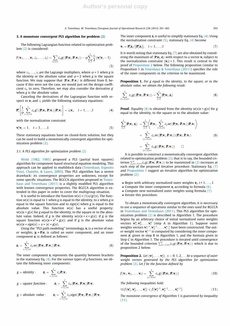
6.2.1.2. Application to the wine tasting experiment. Results of PCA onthe whole dataset are given in Table 6. We decide to study in thissection the set of sub-blocks built with variables correlated to thefirst principal component and to global quality.

6.2.2. Step 2: Modeling the relations between sub-blocksWe may use the SUMCOV method (see Table 2) to relate the

sub-blocks. The following optimization problem is considered:

Maximizew1 ;...;w4

X4

j;k¼1;j–k

CovðXjwj;XkwkÞ

s:c: kwjk ¼ 1; j ¼ 1; . . . ;4:

ð27Þ

RGCCA with mode A for all blocks and g equals to the identity isused to solve optimization problem (27). This problem (27) canbe considered as an ‘‘average’’ one-component PLS regression be-tween the various pairs of blocks Xj and Xk.

6.2.2.1. Application to the wine tasting experiment. The multiblockanalysis has been carried out with the RGCCA R package (Tenen-haus & Guillemot, 2013). RGCCA is also available in the PLS-PM op-tion of the XLSTAT software (Addinsoft, 2013). Using the SUMCOVcriterion on the set of sub-blocks selected in step 1, we obtain theresults given in Fig. 1. Based on a bootstrap strategy, all correla-tions which appear in Fig. 1 are significant.

6.2.2.2. Graphical displays. We summarize all the variables appear-ing in Fig. 1 by their standardized first principal component. Usingthis component (labeled Factor 1) and global quality, we obtain thegraphical display shown in Fig. 2: wines are visualized using soilmarkers (actually, appellation is not a good indicator of qualityfor these Loire wines). High quality wines coming from the refer-ence soil are well recognized by the experts. The reader interestedin wine can even detect that the Saumur 1DAM is one of the bestwines from this sample. We can testify that we drank outstandingSaumur-Champigny produced at Dampierre-sur-Loire.

6.2.2.3. Discussion. The selected variables are related to global qual-ity. RGCCA for multiblock data analysis brings out the fact that ex-perts are able to connect the four sub-blocks described in Fig. 1.They are able to predict the taste of wine from a three-step inspec-tion: (1) olfaction at rest, (2) view and (3) olfaction after shaking. Forexample, harmony (tasting9) is well correlated to its block compo-nent (corr =.963) and also to the other block paragons: correlation ofharmony with aromatic quality at rest (rest2) is equal to .672; withvisual intensity (view1) correlation is equal to .806; and with aro-matic quality in mouth (shaking10) correlation is equal to .808.

7. Application of RGCCA to multigroup data analysis

De Roover, Ceulemans, Timmerman, Vansteelandt et al. (2012)illustrated and motivated Clusterwise SCA-ECP through an exam-ple stemming from social psychology. In this section, RGCCA for



multigroup data analysis and Clusterwise SCA-ECP are compared ina simplified version of this example.

7.1. Description of the example

This example is related to the public good dilemma. Public goodsare goods where everyone will gain a benefit if the good is pro-duced, whether they pay for it or not. Those who pay for the publicgood are named cooperators and those who do not pay are namedfree-riders. The example describes the emotional reactions of 282

participants (playing the role of cooperators) in the presence offree-riders under various equality/empathy conditions. Both play-ers receive a reward. In the equality condition (E), the rewards forthe cooperator and the free-rider are equal, but in the unequal con-dition (UE) the free-rider receives a higher reward. Some informa-tion on the free-rider is eventually given to the cooperator. In thehigh empathy condition (HE), the cooperator receives a messageabout a negative personal event that happened to the free-riderand is asked to imagine how the free-rider feels. In the low empathycondition (LE), the cooperator also receives a message, but is asked

Table 6Correlations of variables with global quality and principal components. Significant correlations are highlighted in bold; in the component part of the Table, only the largestcorrelation of each row is indicated in bold (except for vegetable note).

Global quality Component

1 2 3 4 5

Aromatic quality at rest rest2 .616 .810 �.033 �.365 .076 �.012Fruity note at rest rest3 .495 .683 �.116 �.585 .174 .126Visual intensity view1 .539 .870 .265 .104 �.125 �.237Shading view2 .508 .851 .265 .099 �.179 �.242Surface impression view3 .673 .946 .100 �.065 �.028 �.142Smell quality shaking2 .759 .804 �.351 �.281 .126 �.012Fruity note shaking3 .654 .728 �.300 �.526 .096 .009Aromatic intensity in mouth shaking8 .608 .902 .055 �.112 .250 �.159Aromatic persistence in mouth shaking9 .678 .930 .137 .134 .141 .213Aromatic quality in mouth shaking10 .851 .776 �.531 �.089 �.041 .136Intensity of attack tasting1 .770 .869 .047 .185 �.261 .188Astringency tasting3 .411 .786 .489 .149 �.136 �.017Alcohol tasting4 .524 .788 .234 �.140 .069 .040Balance tasting5 .951 .817 �.496 .076 �.088 .014Mellowness tasting6 .916 .867 �.405 .125 �.101 �.052Ending intensity tasting8 .796 .942 .065 .089 �.175 .163Harmony tasting9 .875 .930 �.232 .159 �.156 �.049Vegetable note shaking6 �.820 �.554 .634 .023 .399 �.106Smell intensity at rest rest1 .037 .533 .695 �.038 .186 .017Spicyl note at rest rest5 �.307 .004 .816 .146 �.323 .213Smell intensity shaking1 .175 .601 .620 .195 .283 �.009Spicy note shaking5 �.081 .262 .715 �.018 �.289 .047Bitterness tasting7 .047 .362 .684 .092 �.046 .104Floral note at rest rest4 .509 .457 �.355 .571 .393 .158Floral note shaking4 .592 .231 �.570 .627 .163 .372Phenolic note shaking7 .086 .382 .354 .185 .560 �.200Acidity tasting2 �.338 �.198 .400 �.390 .138 .702

Fig. 1. SUMCOV on related sub-blocks. (Numbers appearing in this figure are correlations between variables and block components or between two block components.)



to take an objective perspective. In the control condition (C), thecooperator does not receive any message. The two equality condi-tions (E/UE) are fully crossed with the three empathy conditions(HE/LE/C). The 282 participants are partioned in 6 equality/empa-thy groups and are asked how they feel about 21 emotion terms.Using the results of De Roover et al., we have simplified the exampleby selecting 8 emotion terms only: Frustated, Fearful, Surprised,Happy, Satisfied, Sympathetic, Tenderhearted, Tender. These termshave been selected from Table 6 of their paper in order to maintainthe same similarities and differences between equal and unequalconditions groups while limiting redundancy. RGCCA for multi-group data analysis is used on this simplified example.

7.2. Using RGCCA for multigroup data analysis

The whole data matrix X is partitioned into 6 groups: X1 for the47 participants of the E/HE group, X2 for the 46 participants of theE/LE group, X3 for the 48 participants of the E/C group, X4 for the 47participants of the UE/HE group, X5 for the 48 participants of theUE/LE group and X6 for the 46 participants of the UE/C group. Eachcolumn j of each group i is centered and normalized. In addition, asuper-group X7 is obtained by row concatenation of the 6 groups Xi

and division byffiffiffi6p

.RGCCA for multigroup data analysis is sequential. A first

common dimension to the 6 groups is sought by considering thefollowing optimization problem:

Maximizew1 ;...;w7

X6

i¼1

cosðXti Xiwi;X

t7X7w7Þ � Xt

i Xiwi

� Xt7X7w7

s:c: kXiwik ¼ 1; i ¼ 1; . . . ;7:

ð28Þ

This optimization problem is similar to situation 3 above, but with gequal to the identity instead of the square function. Therefore opti-mization problem (28) yields a compromise between PCA of eachgroup and of the super-group and small angles between group-loading vectors and the super-group-loading vector. The obtainedloading vectors Xt

i Xiw1i are given in Table 7.

The average variance explained (AVE) by a component is de-fined as the mean of the square correlations between the variablesand the component. We notice that the ratios AVE(RGCCA)/AVE(PCA)as well as the cosines between the group-loading vectors and thesuper-group-loading vector are fairly high for all groups. We alsonotice that the super-group component is very close to the firstprincipal component of the super-group (very close AVE). Optimi-zation problem (28) (the g function is equal to the identity) andoptimization problem (20) (g is the square function) yield verysimilar results.

Then, second components orthogonal to the previous ones areobtained by considering the following optimization problem:

Maximizew1 ;...;w7

X6

i¼1

cosðXti Xiwi;X

t7X7w7Þ � Xt

i Xiwi

� Xt7X7w7

s:c: kXiwik ¼ 1 and wt

i Xti Xiw1

i ¼ 0; i ¼ 1; . . . ;7

ð29Þ

Optimization problem (29) is solved by deflation as explained inSection 5.1. The second dimension group-loading vectors Xt

i Xiw2i

are given in Table 8. All cosines between the group-loading vectors(dim 2) and the super-group-loading vector (dim 2) are fairly highfor all groups. We may notice that the ratios AVE(RGCCA)/AVE(PCA)for two components are all close to 1.

The use of RGCCA described here is closer to SCA-ECP (or toSCA-IND) than to SCA-P because orthogonal group and super-group components have been sought.

We now study the proximities between groups with respect totheir loadings. Due to the method used, all group-loading vectorsfor dimensions 1 and 2 are pointing out in the same direction.More precisely, the cosines between group-loading vectors givenin Table 7 for dimension 1 and in Table 8 for dimension 2 are allpositive. Therefore, it makes sense to row concatenate group-loading vectors for dimensions 1 and 2. Cosines between these vec-tors measure similarities between groups and are given in Table 9.A partition of the 6 groups into two clusters (Equal vs. Unequalconditions) clearly appears in Table 9 and Fig. 3: the correlationstructures between the 8 variables are more similar withinequality conditions than between equality conditions.

To better identify the difference between equal and unequalconditions with respect to correlation structure, separate PCA arecarried out with oblique rotation for each equality condition.

Fig. 2. Graphical display of wine observations labeled by soil.

Table 7Group-loadings (dimension 1). (Loadings are highlighted in bold in accordance with Table 10.)

E/HE E/LE E/C UE/HE UE/LE UE/C global_1

satisfied 0.802 0.823 0.896 0.911 0.875 0.656 0.831happy 0.808 0.818 0.852 0.894 0.893 0.738 0.835frustrated �0.660 �0.853 �0.943 �0.810 �0.793 �0.725 �0.800fearful �0.696 �0.748 �0.806 �0.001 �0.285 �0.279 �0.476sympathetic �0.016 0.234 0.311 0.313 0.091 0.106 0.178surprised �0.401 �0.311 �0.409 �0.521 �0.671 �0.403 �0.453tenderhearted �0.118 �0.229 �0.207 0.054 �0.015 0.180 �0.063tender 0.237 0.135 0.099 0.588 0.377 0.079 0.255

AVE(RGCCA) 0.306 0.357 0.423 0.375 0.359 0.224 0.320AVE(PCA) 0.320 0.367 0.434 0.411 0.365 0.242 0.321AVE(RGCCA)/AVE(PCA) 0.955 0.974 0.975 0.914 0.985 0.923 0.998Cos(group, global 1) 0.978 0.975 0.976 0.934 0.981 0.973



Correlations between the data normalized by group and the ro-tated factors are given in Table 10.

Five items have similar loadings on both components for thetwo clusters. These 5 items also have similar loadings across the6 groups (they are put in bold normal in Tables 7, 8 and 10). Usingthese 5 items, the interpretation of components is similar for bothclusters: first component opposes positive affect (happy, satisfied)to negative affect (frustrated); second component is related toempathy (tenderhearted, tender). However, a very different load-ing pattern across the two clusters is found for three emotions:fearful, surprised and sympathetic (they are put in bold italic in Ta-bles 7, 8 and 10). As De Roover et al. obtained very similar resultsusing Clusterwise SCA-ECP on the complete dataset, we may sum-marize their interpretation of these differences:

(1) Fearful is negatively correlated to the first component in theequal condition cluster; therefore it is a negative affect forthis cluster. Fearful is positively correlated to the secondcomponent in the unequal condition cluster; people of thiscluster who react empathically also feel fearful (more detailson this point are given in De Roover et al.).

(2) Sympathetic is uncorrelated to both components in theequal condition cluster. Sympathetic is positively correlatedto the emotion component in the unequal condition cluster;people of this cluster who react with sympathy to the free-riders because they take into account some negative per-sonal event that happened to them also feel tenderhearted.

(3) Surprise is positively correlated to the empathy componentin the equal condition cluster. Therefore in this cluster, it isa positive emotion. Surprise is negatively correlated to thefirst component in the unequal condition cluster. In this clus-ter this emotion is negative and associated with frustration.

7.3. Comparison with Clusterwise SCA-ECP

Clusterwise SCA-ECP is defined in De Roover, Ceulemans, andTimmerman (2012). They consider the following optimizationproblem:

MaximizeW1 ;...;WI ;P1 ;...;PK

g11 ;...;gIK

XI

i¼1

Xi �XK

k¼1

gikXiWiPtk

2

s:c: ð1=niÞWti X

ti XiWi ¼ I; i ¼ 1; . . . ; I

ð30Þ

where Wi is a p � q (q < p) weight matrix related to groupXi, i = 1,. . ., I, Pk a p � q pattern matrix related to cluster k,

Fig. 3. Hierarchical cluster analysis based on Table 9.

Table 9Cosines between group-loading vectors (dimension 1 + 2). Cosines between group-loading vectors related to the same equal/unequal condition are indicated in bold.

Group E/HE E/LE E/C UE/HE UE/LE UE/C

E/HE 1.000 .971 .933 .870 .897 .935E/LE .971 1.000 .980 .877 .906 .926E/C .933 .980 1.000 .866 .871 .873UE/HE .870 .877 .866 1.000 .961 .916UE/LE .897 .906 .871 .961 1.000 .956UE/C .935 .926 .873 .916 .956 1.000

Table 8Group-loadings (dimension 2). (Loadings are highlighted in bold in accordance with Table 10.)

E/HE E/LE E/C UE/HE UE/LE UE/C global_2

satisfied 0.239 0.252 0.109 0.105 0.194 0.147 0.177happy 0.198 0.177 0.165 0.058 0.136 0.172 0.153frustrated 0.352 0.287 0.064 �0.066 0.093 0.308 0.176fearful 0.128 0.324 0.278 0.460 0.658 0.354 0.395sympathetic 0.683 0.458 0.166 0.583 0.764 0.801 0.583surprised 0.612 0.416 0.477 0.353 0.174 0.211 0.367tenderhearted 0.845 0.762 0.767 0.842 0.780 0.667 0.785tender 0.741 0.710 0.749 0.547 0.410 0.567 0.635

AVE(RGCCA) (dim 2) 0.293 0.219 0.191 0.213 0.236 0.215 0.217AVE(PCA) (dim 2) 0.286 0.217 0.220 0.192 0.253 0.221 0.217AVE(RGCCA) (dim 1 + 2) 0.599 0.576 0.614 0.588 0.595 0.439 0.537AVE(PCA) (dim 1 + 2) 0.606 0.584 0.654 0.603 0.618 0.463 0.538AVE(RGCCA)/AVE(PCA) 0.988 0.986 0.939 0.976 0.984 0.948 0.999Cos(group, global 2) 0.963 0.986 0.931 0.974 0.946 0.968

Table 10Structure matrix for equal and unequal conditions. Significant correlations areindicated in bold; items with very different correlations in the equal and unequalcondition groups are indicated in italics. (Separate PCA followed by oblique rotation.)

Correlations between normalized data and rotated factors

Equal conditions Unequal conditionsComponent Component

1 2 1 2

Satisfied .834 .161 .817 .221Happy .821 .172 .850 .197Frustrated �.831 .276 �.773 �.002Fearful �.785 .237 �.074 .575Sympathetic .215 .277 .124 .789Surprised �.297 .621 �.610 .099Tenderhearted �.162 .789 .062 .761Tender .175 .780 .369 .464



k = 1, . . . , K and gik = 1 if group Xi belongs to cluster k and gik = 0otherwise. We have used the Multiblock component analysis(MBCA) software (downloaded from http://ppw.kuleuven.be/okp/software/MBCA/) on the above example for q = 2 and K = 1 to 6.For K = 1 cluster, optimization problem (30) corresponds to SCA-ECP. For K = 6 clusters, optimization problem (30) corresponds toseparate PCA on each group Xi.

Denoting by LK the loss function in (30), the percentage of var-iance accounted for (VAF) is defined in De Roover et al. by

VAFðKÞ ¼PI

i¼1kXik2 � LKPIi¼1kXik2 � 100 ð31Þ

De Roover et al. select the optimal number of clusters by using themaximal value of the Scree ratio defined by

SRðKÞ ¼ VAFðKÞ � VAFðK � 1ÞVAFðK þ 1Þ � VAFðKÞ ð32Þ

Values of VAF and SR for K = 1 to 6 are given in Table 11. This leadsto the choice of two clusters. The first cluster contains all equal con-ditions and the second cluster all unequal conditions. Therefore,RGCCA and Clusterwise SCA-ECP lead to the same two clusters onthis example. The oblique rotation option has been selected in theMBCA program. Correlations between the normalized data andthe rotated factors are given in Table 12. Comparing Tables 10and 12, we may conclude that PCA and SCA-ECP (both followedby an oblique rotation) give very similar results on this example.Both methods reveal the basic structure of the data.

8. Conclusion

In this paper, the distinction between multiblock and multi-group data analysis is clearly defined. Multiblock data concernsthe case of several sets of variables observed on the same individ-uals, while multigroup data concerns the situation where the samevariables are observed on several sets of individuals. The main aimof multiblock data analysis is to investigate the relationships be-tween blocks, while the main aim of multigroup data analysis is

to investigate the relationships among variables within the variousgroups. We have shown in this paper that a single simple and pow-erful algorithm can be used for both multiblock and multigroupdata. In the multiblock situation, RGCCA is applied on the blocksX0j s while in the multigroup situation it is applied on the within-group correlation matrices R0i s.

Much experience has been accumulated in multiblock dataanalysis and an overview of these methods is presented from aRGCCA perspective. The novelty of this paper concerns the exten-sion of RGCCA to the multigroup situation. RGCCA for multigroupdata analysis is based on the idea of carrying out connected PCA’son the various groups of individuals.

It is worth pointing out that PCA plays a central role in multi-block and multigroup data analysis. Well-known reference meth-ods such as Consensus PCA for multiblock data and SCA-P formultigroup data boil down to a PCA of the whole data table (afterpreprocessing) and are both a special case of RGCCA.

We have illustrated RGCCA for multiblock data on a wine test-ing example. We have compared RGCCA for multigroup data andClusterwise SCA-ECP on an example from the field of socialpsychology.

Acknowledgements

We would like to gratefully thank the three anonymous refereesfor their comments which have greatly improved our manuscript.

Appendix A. Proof of proposition 2

The proof of Proposition 2 relies on the following lemma, wherethe outer weight vectors vs

i and the inner component zsi are defined

in Algorithm 1:

Lemma 1. For i = 1, . . ., I, s = 0, 1, 2, . . ., let f si be the function defined

by

f si ðviÞ ¼

X‘i

ci‘g Pivi;P‘vs‘

�� Then the following property holds:

8s f si vs

i

� �6 f s

i vsþ1i

� �ð33Þ

Proof of Lemma 1. The function f si vs

i

� �may be written as

f si vs

i

� �¼X‘i

ci‘g Pivsi ;P‘vs

‘

�� ¼X‘i

ci‘w Pivsi ;P‘vs

‘

�� Pivs

i ;P‘vs‘

�

¼ Pivsi ;X‘i


‘

�� P‘vs

‘

* +

¼ Pivsi ;z

si

�ð34Þ

Using the definitions of zsi and vsþ1

i , the following inequality holds:

f si vs

i

� �¼ Pivs

i ; zsi

�6 Pivsþ1

i ; zsi

�ð35Þ

and we get the equality

Pivsþ1i ; zs

i

�¼X‘i


‘

�� Pivsþ1

i ;P‘vs‘

�ð36Þ

Table 11Clusterwise SCA-ECP: Fit values for the analyses.

Number of clusters VAF (K) SCREE ratio

1 53.002 56.10 2.953 57.15 1.214 58.02 1.715 58.53 1.506 58.87

Table 12Structure matrix for equal and unequal conditions. Significant correlations areindicated in bold; items with very different correlations in the equal and unequalcondition groups are indicated in italics. (SCA-ECP followed by oblique rotation.)

Correlations between normalized data and rotated factors

Equal conditions Unequal conditionsComponent Component

1 2 1 2

Satisfied 0.826 0.103 0.815 0.220Happy 0.816 0.120 0.856 0.200Frustrated �0.837 0.317 �0.762 �0.005Fearful �0.790 0.293 �0.049 0.561Sympathetic 0.184 0.230 0.154 0.788Surprised �0.320 0.640 �0.607 0.097Tenderhearted �0.185 0.795 0.104 0.770Tender 0.156 0.774 0.359 0.460



Then, we have to consider separately the three types of function g.g = identity and w (x) = 1In this situation, equality (36) becomes

Pivsþ1i ; zs

i

�¼X‘i

ci‘ Pivsþ1i ;P‘vs

‘

�¼ f s

i vsþ1i

� �ð37Þ

and therefore f si vs

i

� �6 f s

i vsþ1i

� �.

g = absolute value and w(x) = sign(x)In this situation, equalities (34) and (36) become respectively

f sj vs

i

� �¼X‘i

ci‘ Pivsi ;P‘vs

‘

�� ð38Þ

and

Pivsþ1i ; zs

i

�¼X‘i

ci‘sign Pivsi ;P‘vs

‘

�� Pivsþ1

i ;P‘vs‘

�ð39Þ

Therefore, we obtain

f si vs

i

� �¼ f s

i vsi

� �� 6 Pivsþ1i ; zs

i

�¼ Pivsþ1

i ; zsi

�� 6

X‘i


‘

�� ¼ f s

i vsþ1i

� �ð40Þ

g = square function and w(x) = xIn this situation, equalities (34) and (36) become respectively

f si vs

i

� �¼X‘i

ci‘ Pivsi ;P‘vs

‘

�2 ð41Þ

and

Pivsþ1i ; zs

i

�¼X‘i

ci‘ Pivsi ;P‘vs

‘

�Pivsþ1

i ;P‘vs‘

�ð42Þ

The right term of (42) is the scalar product between two vectors.Using the Cauchy–Schwartz inequality and the fact that c2

i‘ ¼ ci‘,we obtain

Pivsþ1i ; zs

i

�6

X‘i

ci‘ Pivsi ;P‘vs

‘

�2

" #1=2

�X‘i


‘

�2

" #1=2

ð43ÞFrom that we deduce

f si vs

i

� �6 f s

i vsi

� �� 1=2 f si vsþ1

i

� �� 1=2 ð44Þand therefore

f si vs

i

� �6 f s

i vsþ1i

� �� ð45Þ

Proof of Proposition 1. Proposition 2 is deduced from lemma 1and the following equality:

XI

i¼1

f si vsþ1

i

� �� f s

i vsi

� �� ¼XI

i¼1

X‘i

ci‘g Pivsþ1i ;P‘vs

‘

�� X‘i


‘

�� #¼XI

i¼1

X‘i


‘

�� #¼1

2

XI

i;‘¼1;i–‘


‘

�� 1

2

XI

i;‘¼1;i–‘


‘

�� ¼1

2f vsþ1

1 ; . . . ;vsþ1I

� �� f vs

1; . . . ;vsI

� ��

References

Addinsoft (2013). XLSTAT software. Paris.Carroll, J. D. (1968a). A generalization of canonical correlation analysis to three or

more sets of variables. Proceedings of the 76th Annual Convention of the AmericanPsychological Association, 227–228.

Carroll, J. D. (1968b). Equations and tables for a generalization of canonical correlationanalysis to three or more sets of variables. Unpublished companion paper toCarroll, J.D. (1968a).

Chessel, D., & Hanafi, M. (1996). Analyses de la co-inertie de Knuages de points.Revue de Statistique Appliquée, 44, 35–60.

De Roover, K., Ceulemans, E., & Timmerman, M. E. (2012). How to perform multiblockcomponent analysis in practice. Behavior Research Methods, 44, 41–56.

De Roover, K., Ceulemans, E., Timmerman, M. E., & Onghena, P. (2013). A clusterwisesimultaneous component method for capturing within-cluster differences incomponent variances and correlations. British Journal of Mathematical andStatistical Psychology, 66, 81–102.

De Roover, K., Ceulemans, E., Timmerman, M. E., Vansteelandt, K., Stouten, J., &Onghena, P. (2012). Clusterwise simultaneous component analysis foranalyzing structural differences in multivariate multiblock data. PsychologicalMethods, 17, 100–119. http://dx.doi.org/10.1037/a0025385.

De Roover, K., Timmerman, M. E., Van Mechelen, I., & Ceulemans, E. (2013). On theadded value of multiset methods for three-way data analysis. Chemometrics andIntelligent Laboratory Systems, 129, 98–107.

Eslami, E., Qannari, E. M., Kohler, A., & Bougeard, S. (2013a). General overview ofmethods of analysis of multi-group datasets. Revue des Nouvelles Technologies del’Information, 25, 108–123.

Eslami, E., Qannari, E. M., Kohler, A., & Bougeard, S. (2013b). Analyses factorielles dedonnées structurées en groupes d’individus. Journal de la Société Française deStatistique, 154, 44–57.

Flury, B. N. (1984). Common principal components in k groups. Journal of theAmerican Statistical Association, 79, 892–898.

Flury, B. N. (1987). Two generalizations of common principal component model.Biometrika, 74, 59–69.

Hanafi, M. (2007). PLS path modelling: Computation of latent variables with theestimation mode B. Computational Statistics, 22, 275–292.

Hanafi, M., & Kiers, H. A. L. (2006). Analysis of K sets of data, with differentialemphasis on agreement between and within sets. Computational Statistics &Data Analysis, 51, 1491–1508.

Hanafi, M., Kohler, A., & Qannari, E. M. (2010). Shedding new light on hierarchicalprincipal component analysis. Journal of Chemometrics, 24, 703–709.

Hanafi, M., Kohler, A., & Qannari, E. M. (2011). Connections between multiple co-inertia analysis and consensus principal component analysis. Chemometrics andIntelligent Laboratory Systems, 106, 37–40.

Hanafi, M., Mazerolles, E., Dufour, E., & Qannari, E. M. (2006). Common componentsand specific weight analysis and multiple co-inertia analysis applied to thecoupling of several measurement techniques. Journal of Chemometrics, 20,172–183.

Hassani, S., Hanafi, M., Qannari, E. M., & Kohler, A. (2013). Deflation strategies formulti-block principal component analysis revisited. Chemometrics andIntelligent Laboratory Systems, 120, 68.

Horst, P. (1961). Relations among m sets of variables. Psychometrika, 26, 126–149.Hotelling, H. (1936). Relations between two sets of variates. Biometrika, 28,

321–377.Kettenring, J. R. (1971). Canonical analysis of several sets of variables. Biometrika,

58, 433–451.Kiers, H. A. L. (1991). Hierarchical relations among three-ways methods.

Psychometrika, 56, 449–470.Kiers, H. A. L., & Ten Berge, J. M. F. (1989). Alternating least squares algorithms for

simultaneous components analysis with equal component weight matrices intwo or more populations. Psychometrika, 54, 467–473.

Kiers, H. A. L., & Ten Berge, J. M. F. (1994). Hierarchical relations between methodsfor simultaneous component analysis and a technique for rotation to a simplesimultaneous structure. British Journal of Mathematical and Statistical Psychology,47, 109–126.

Krämer, N. (2007). Analysis of high-dimensional data with partial least squares andboosting. Doctoral dissertation, Technischen Universität Berlin.

Krzanowski, W. J. (1979). Between-groups comparison of principal components.Journal of the American Statistical Association, 33, 164–168.

Krzanowski, W. J. (1984). Principal component analysis in the presence of groupstructure. Applied Statistics, 33, 164–168.

Levin, J. (1966). Simultaneous factor analysis of several Gramian matrices.Psychometrika, 31, 413–419.

Niesing, J. (1997). Simultaneous component and factor analysis methods for two ormore groups: a comparative study. M&T series (Vol. 30). Leiden: DSWO Press.

Pagès, J., Asselin, C., Morlat, R., & Robichet, J. (1987). Analyse factorielle multipledans le traitement de données sensorielles: Application à des vins rouges de lavallée de la Loire. Sciences des aliments, 7, 549–571.

Pearson, K. (1901). On lines and planes of closest fit to systems of points in space.Philosophical Magazine, 2, 559–572.

Smilde, A. K., Westerhuis, J. A., & de Jong, S. (2003). A framework for sequentialmultiblock component methods. Journal of Chemometrics, 17, 323–337.

Ten Berge, J. M. F. (1988). Generalized approaches to the MAXBET problem and theMAXDIFF problem, with applications to canonical correlations. Psychometrika,53, 487–494.



Tenenhaus, A., & Guillemot, V. (2013). RGCCA Package. <http://cran.project.org/web/packages/RGCCA/index.html>.

Tenenhaus, M., & Esposito Vinzi, V. (2005). PLS regression, PLS path modeling andgeneralized Procrustean analysis: A combined approach for multiblock analysis.Journal of Chemometrics, 19, 145–153.

Tenenhaus, M., Esposito Vinzi, V., Chatelin, Y.-M., & Lauro, C. (2005). PLS pathmodeling. Computational Statistics & Data Analysis, 48, 159–205.

Tenenhaus, M., & Hanafi, M. (2010). A bridge between PLS path modelling andmultiblock data analysis. In V. Esposito Vinzi, J. Henseler, W. Chin, & H. Wang(Eds.), Handbook of partial least squares (PLS): Concepts, methods and applications(pp. 99–123). Springer Verlag.

Tenenhaus, A., & Tenenhaus, M. (2011). Regularized generalized canonicalcorrelation analysis. Psychometrika, 76, 257–284.

Timmerman, M. E., & Kiers, H. A. L. (2003). Four simultaneous component modelsfor the analysis of multivariate time series from more than one subject to modelintra-individual and inter-individual differences. Psychometrika, 68, 105–121.

Tucker, L. R. (1958). An inter-battery method of factor analysis. Psychometrika, 23,111–136.

Van de Geer, J. P. (1984). Linear relations among k sets of variables. Psychometrika,49, 70–94.

van den Wollenberg, A. L. (1977). Redundancy analysis – An alternative to canonicalcorrelation analysis. Psychometrika, 42, 207–219.

Van Deun, K., Smilde, A. K., van der Werf, M. J., Kiers, H. A. L., & Van Mechelen, I.(2009). A structured overview of simultaneous component based dataintegration. BMC Bioinformatics, 10, 246.

Westerhuis, J. A., Kourti, T., & MacGregor, J. F. (1998). Analysis of multiblock andhierarchical PCA and PLS models. Journal of Chemometrics, 12, 301–321.

Wold, H. (1982). Soft modeling: The basic design and some extensions. In K. G.Jöreskog & H. Wold (Eds.), Systems under indirect observation, Part 2 (pp. 1–54).Amsterdam: North-Holland.

Wold, H. (1985). Partial least squares. In S. Kotz & N. L. Johnson (Eds.). Encyclopediaof statistical sciences (vol. 6, pp. 581–591). New York: John Wiley & Sons.

Wold, S., Hellberg, S., Lundstedt, T., Sjostrom, M., & Wold, H. (1987). PLS modellingwith latent variables in two or more dimensions. In Proceedings of thesymposium on PLS model building: Theory and application (pp. 1–21). Germany:Frankfurt am Main.

Documents

Multigroup or multiblock data analysis with RGCCA (PDF Download