Embed Size (px)
Citation preview

MULTIGRID METHODS WITH SPACE-TIME CONCURRENCY
R. D. FALGOUT† , S. FRIEDHOFF‡§ , TZ. V. KOLEV† ,
S. P. MACLACHLAN¶, J. B. SCHRODER† , AND S. VANDEWALLE‡
Abstract. We consider the comparison of multigrid methods for parabolic partial differentialequations that allow space-time concurrency. With current trends in computer architectures leadingtowards systems with more, but not faster, processors, space-time concurrency is crucial for speedingup time-integration simulations. In contrast, traditional time-integration techniques impose seriouslimitations on parallel performance due to the sequential nature of the time-stepping approach, al-lowing spatial concurrency only. This paper considers the three basic options of multigrid algorithmson space-time grids that allow parallelism in space and time: coarsening in space and time, semi-coarsening in the spatial dimensions, and semicoarsening in the temporal dimension. We discussadvantages and disadvantages of the different approaches and their benefit compared to traditionalspace-parallel algorithms with sequential time stepping on modern architectures.
Key words. multigrid methods; space-time discretizations; parallel-in-time integration
AMS subject classifications. 65F10, 65L06, 65M55, 65N22
1. Introduction. The numerical solution of linear systems arising from the dis-cretization of partial differential equations (PDEs) with evolutionary behavior, such asparabolic (space-time) problems, hyperbolic problems, and equations with time-likevariables is of interest in many applications including fluid flow, magnetohydrody-namics, compressible flow, and charged particle transport. Current trends in super-computing leading towards computers with more, but not faster, processors inducea change in the development of algorithms for these type of problems. Instead ofexploiting increasing clock speeds, faster time-to-solution must come from increasingconcurrency, driving the development of time-parallel and full space-time methods.
In contrast to classical time-integration techniques based on a time-stepping ap-proach, i.e., solving sequentially for one time step after the other, time-parallel andspace-time methods allow simultaneous solution across multiple time steps. As aconsequence, these methods enable exploitation of substantially more computationalresources than standard space-parallel methods with sequential time stepping. Whileclassical time-stepping has optimal algorithmic scalability, with best possible com-plexity when using a scalable solver for each time step, space-time-parallel methodsintroduce more computations and/or memory usage to allow the use of vastly moreparallel resources. In other words, space-time parallel methods remain algorithmi-cally optimal, but with larger constant factors. Their use provides a speedup overtraditional time-stepping when sufficient parallel resources are available to amortize
†Center for Applied Scientific Computing, Lawrence Livermore National Laboratory, P. O. Box808, L-561, Livermore, CA 94551 (rfalgout, tzanio, [email protected]). This work performedunder the auspices of the U.S. Department of Energy by Lawrence Livermore National Laboratoryunder Contract DE-AC52-07NA27344 (LLNL-JRNL-678572).
‡Department of Computer Science, KU Leuven, Celestijnenlaan 200a - box 2402, 3001 Leuven,Belgium ([email protected]). SF and SV acknowledge support from OPTEC (OP-Timization in Engineering Center of excellence KU Leuven), which is funded by the KU LeuvenResearch Council under grant no. PFV/10/002.
§Current address: Mathematisches Institut, Universitat zu Koln, Weyertal 86-90, 50931 Koln,Germany ([email protected]).
¶Department of Mathematics and Statistics, Memorial University of Newfoundland, St. John’s,NL, Canada ([email protected]). The work of SM was partially supported by an NSERC discov-ery grant.
1

2 R. D. Falgout, S. Friedhoff, Tz. V. Kolev, S. P. MacLachlan, J. B. Schroder, S. Vandewalle
their increased cost.
Research on parallel-in-time integration started about 50 years ago with the semi-nal work of Nievergelt in 1964 [36]. Since then, various approaches have been explored,including direct methods such as [9,20,33,35,39], as well as iterative approaches basedon multiple shooting, domain decomposition, waveform relaxation, and multigrid in-cluding [4, 8, 10, 11, 17, 21, 24–28, 31, 32, 34, 41–45]. A recent review of the extensiveliterature in this area is [16]. In this paper, we focus on multigrid approaches.
The use of multigrid for adding parallelism to time integration allows for fastertime-to-solution in comparison with classical time-stepping approaches, given enoughcomputational resources available [11, 17, 44]. A comparison of the different space-time-parallel approaches, however, does not exist. In this paper, we consider a com-parison of the three basic options for multigrid on space-time grids: coarsening inspace and time, semicoarsening only in the spatial dimensions, and semicoarseningonly in the temporal dimension. More specifically, we compare space-time multi-grid (STMG) [26], space-time concurrent multigrid waveform relaxation with cyclicreduction (WRMG-CR) [27], and multigrid-reduction-in-time (MGRIT) [11] for timediscretizations using backward differences of order k (BDF-k). While many variationson these and other approaches are possible, they represent the most basic choices formultigrid methods on space-time grids.
The goal of our comparison is not to simply determine the algorithm with thefastest time-to-solution for a given problem. Instead, we aim at determining advan-tages and disadvantages of the methods based on comparison parameters such asrobustness, intrusiveness, storage requirements, and parallel performance. We recog-nize that there is no perfect method, since there are necessarily trade-offs betweentime-to-solution for a particular problem, robustness, intrusiveness, and storage re-quirements. One important aspect is the effort one has to put into implementing themethods when aiming at adding parallelism to an existing time-stepping code. WhileMGRIT is a non-intrusive approach that, similarly to time stepping, uses an existingtime propagator to integrate from one time to the next, both STMG and WRMG-CRare invasive approaches. On the other hand, the latter two approaches have better al-gorithmic complexities than the MGRIT algorithm. In this paper, we are interested inanswering the question of how much of a performance penalty one might pay in usinga non-intrusive approach, such as MGRIT, in contrast with more optimal approacheslike STMG and WRMG-CR. Additionally, we demonstrate the benefit compared toclassical space-parallel time-stepping algorithms in a given parallel environment.
This paper is organized as follows. In Section 2, we review the three multigridmethods with space-time concurrency, STMG, WRMG-CR, and MGRIT, includinga new description of the use of MGRIT for multistep time integration. In Section3, we construct a simple model for the comparison. We introduce a parabolic testproblem, derive parallel performance models, and discuss parallel implementations aswell as storage requirements of the three methods. Section 4 starts with weak scalingstudies, followed by strong scaling studies comparing the three multigrid methodsboth with one another and with a parallel algorithm with sequential time stepping.Additionally, we include a discussion of insights from the parallel models as well asan overview of current research in the XBraid project [2] to incorporate some of themore intrusive, but highly efficient, aspects of methods like STMG. Conclusions arepresented in Section 5.
2. Multigrid on space-time grids. The naive approach of applying multi-grid with standard components, i.e., point relaxation and full coarsening, for solving

Multigrid methods with space-time concurrency 3
parabolic (space-time) problems typically leads to poor multigrid performance (see,e.g. [26]). In this section, we describe three multigrid algorithms that offer goodperformance, allowing parallelism in space and time. For a given parabolic prob-lem, the methods assume different discretization approaches using either a point-wisediscretization of the whole space-time domain or a semidiscretization of the spatialdomain. However, for a given discretization in both space and time, all methods solvethe same (block-scaled) resulting system of equations.
2.1. Space-time multigrid. The space-time multigrid (STMG) method [26]treats the whole of the space-time problem simultaneously. The method uses pointsmoothers and employs a parameter-dependent coarsening strategy that chooses eithersemicoarsening in space or in time at each level of the hierarchy.
Let Σ = Ω×[0, T ] be a space-time domain and consider a time-dependent parabolicPDE of the form
(2.1) ut +L(u) = b
in Σ, subject to boundary conditions in space and an initial condition in time. Fur-thermore, L denotes an elliptic operator and u = u(x, t) and b = b(x, t) are functions ofa spatial point, x ∈ Ω, and time, t ∈ [0, T ]. We discretize (2.1) by choosing appropri-ate discrete spatial and temporal domains. The resulting discrete problem is typicallyanisotropic due to different mesh sizes used for discretizing the spatial and temporaldomains. Consider, for example, discretizing the heat equation in one space dimen-sion and in the time interval [0, T ] on a rectangular space-time mesh with constantspacing ∆x and ∆t, respectively. If we use central finite differences for discretizingthe spatial derivatives and backward Euler (also, first-order backward differentiationformula (BDF1)) for the time derivative, the coefficient matrix of the resulting lin-ear system depends on the parameter λ = ∆t/(∆x)2, which can be considered as ameasure of the degree of anisotropy in the discrete operator.
Analogously to anisotropic elliptic problems, in the parabolic case, there are alsotwo standard approaches for deriving a multigrid method to treat the anisotropy: thestrategy is to either change the smoother to line or block relaxation, ensuring smooth-ing in the direction of strong coupling, or to change the coarsening strategy, usingcoarsening only in the direction where point smoothing is successful. STMG followsthe second approach. The method uses a colored point-wise Gauss-Seidel relaxation,based on partitioning the discrete space-time domain into points of different ‘color’with respect to all dimensions of the problem. That is, time is treated simply as anyother dimension of the problem.
Relaxation is accelerated using a coarse-grid correction based on an adaptiveparameter-dependent coarsening strategy. More precisely, depending on the degreeof anisotropy of the discretization stencil, λ (e.g., λ = ∆t/(∆x)2 in our previousexample), either semicoarsening in space or in time is chosen. The choice for thecoarsening direction is based on a selected parameter, λcrit, which can be chosen, forexample, using Fourier analysis, as was done for the heat equation [26], applying thetwo-grid methods using either semicoarsening in space (when λ ≥ λcrit) or in time(when λ < λcrit). Thus, a hierarchy of coarse grids is created, where going from onelevel to the next coarser level, the number of points is reduced either only in thespatial dimensions or only in the temporal dimension. Rediscretization is used tocreate the discrete operator on each level, and the intergrid transfer operators areadapted to the grid hierarchy. In the case of space-coarsening, interpolation andrestriction operators are the standard ones used for isotropic elliptic problems. For
4 R. D. Falgout, S. Friedhoff, Tz. V. Kolev, S. P. MacLachlan, J. B. Schroder, S. Vandewalle
time-coarsening, interpolation and restriction are only forward in time, transferringno information backward in time.
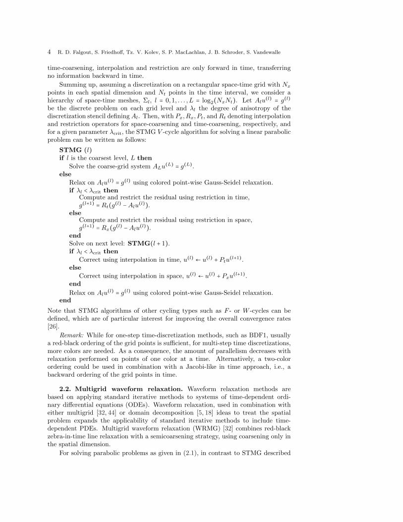
Summing up, assuming a discretization on a rectangular space-time grid with Nxpoints in each spatial dimension and Nt points in the time interval, we consider ahierarchy of space-time meshes, Σl, l = 0,1, . . . , L = log2(NxNt). Let Alu
(l) = g(l)be the discrete problem on each grid level and λl the degree of anisotropy of thediscretization stencil defining Al. Then, with Px,Rx, Pt, andRt denoting interpolationand restriction operators for space-coarsening and time-coarsening, respectively, andfor a given parameter λcrit, the STMG V -cycle algorithm for solving a linear parabolicproblem can be written as follows:
STMG (l)if l is the coarsest level, L then
Solve the coarse-grid system ALu(L) = g(L).
else
Relax on Alu(l) = g(l) using colored point-wise Gauss-Seidel relaxation.
if λl < λcrit thenCompute and restrict the residual using restriction in time,g(l+1) = Rt(g(l) −Alu(l)).
elseCompute and restrict the residual using restriction in space,g(l+1) = Rx(g(l) −Alu(l)).
endSolve on next level: STMG(l + 1).if λl < λcrit then
Correct using interpolation in time, u(l) ← u(l) + Ptu(l+1).else
Correct using interpolation in space, u(l) ← u(l) + Pxu(l+1).end
Relax on Alu(l) = g(l) using colored point-wise Gauss-Seidel relaxation.
end
Note that STMG algorithms of other cycling types such as F - or W -cycles can bedefined, which are of particular interest for improving the overall convergence rates[26].
Remark: While for one-step time-discretization methods, such as BDF1, usuallya red-black ordering of the grid points is sufficient, for multi-step time discretizations,more colors are needed. As a consequence, the amount of parallelism decreases withrelaxation performed on points of one color at a time. Alternatively, a two-colorordering could be used in combination with a Jacobi-like in time approach, i.e., abackward ordering of the grid points in time.
2.2. Multigrid waveform relaxation. Waveform relaxation methods arebased on applying standard iterative methods to systems of time-dependent ordi-nary differential equations (ODEs). Waveform relaxation, used in combination witheither multigrid [32, 44] or domain decomposition [5, 18] ideas to treat the spatialproblem expands the applicability of standard iterative methods to include time-dependent PDEs. Multigrid waveform relaxation (WRMG) [32] combines red-blackzebra-in-time line relaxation with a semicoarsening strategy, using coarsening only inthe spatial dimension.
For solving parabolic problems as given in (2.1), in contrast to STMG described

Multigrid methods with space-time concurrency 5
above, the WRMG algorithm uses a method of lines approximation, discretizing onlythe spatial domain, Ω. Thus, a semidiscrete problem is generated, i.e., the PDE isfirst transformed to a system of time-dependent ODEs of the form
(2.2)d
dtu(t) +Q(u(t)) = b(t), u(0) = g0, t ∈ [0, T ],
where u(t) and b(t) are vector functions of time, t ∈ [0, T ] (i.e., the semidiscrete ana-logues of the functions u and b in (2.1)), with (d/dt)u(t) denoting the time derivativeof the vector u(t), and where Q is the discrete approximation of the operator L in(2.1). In the linear case, considered in the remainder of this section, function Q(⋅) cor-responds to a matrix-vector product. The idea of waveform (time-line) relaxation [30]is to apply a standard iterative method such as Jacobi or Gauss-Seidel to the ODEsystem (2.2). Therefore, let Q = D − L − U be the splitting of the matrix into itsdiagonal, strictly lower, and strictly upper triangular parts; note that D,L, and Umay be functions of time. Then, one step of a Gauss-Seidel-like method for (2.2) isgiven by
(2.3)d
dtu(new)(t)+ (D−L)u(new)(t) = Uu(old)(t)+ b(t), u(new)(0) = g0, t ∈ [0, T ],
with u(old) and u(new) denoting known and to be updated solution values, respectively.That is, one step of the method involves solving Ns linear, scalar ODEs, where Ns isthe number of variables in the discrete spatial domain (e.g., Ns = N2
x if discretizingon a regular square mesh in 2D). Furthermore, if Q is a standard finite differencestencil and a red-black ordering of the underlying grid points is used, the ODE systemdecouples, i.e., each ODE can be integrated separately and in parallel with the ODEsat grid points of the same color.
The performance of Gauss-Seidel waveform relaxation is accelerated by a coarse-grid correction procedure based on semicoarsening in the spatial dimensions. Moreprecisely, discrete operators are defined on a hierarchy of spatial meshes and standardinterpolation and restriction operators as used for isotropic elliptic problems (e.g., full-weighting restriction and bilinear interpolation for 2D problems), allowing the transferbetween levels in the multigrid hierarchy. Parallelism in this algorithm, however, islimited to spatial parallelism. Space-time concurrent WRMG enables parallelismacross time, i.e., parallel-in-time integration of the scalar ODEs in (2.3) that makeup the kernel of WRMG. While in the method described in [44] only some timeparallelism was introduced by using pipelining or the partition method, WRMG withcyclic reduction (WRMG-CR) [27] enables full time parallelism within WRMG.
The use of cyclic reduction within waveform relaxation is motivated by the con-nection of multistep methods to recurrence relations. Therefore, let ti = iδt, i =0,1, . . . ,Nt, be a temporal grid with constant spacing δt = T /Nt, and for i = 1, . . . ,Nt,let un,i be an approximation to un(ti), with the subscript n = 1, . . . ,Ns indicatingthat we consider one ODE of the system. Then, a general k-step time discretizationmethod for a linear, scalar ODE, e.g., one component of the ODE systems in (2.2) or(2.3), with solution variable un and initial condition un(0) = g0 is given by
un,0 = g0
un,i =mini,k
∑s=1
a(n)i,i−sun,i−s + gn,i, i = 1,2, . . . ,Nt.(2.4)

6 R. D. Falgout, S. Friedhoff, Tz. V. Kolev, S. P. MacLachlan, J. B. Schroder, S. Vandewalle
That is, the solution, un,i, at time ti depends on solution-independent terms, gn,i,e.g., related to boundary conditions or source terms or connections to different spa-tial points, as well as on the solution at the previous k time steps, except at thebeginning, where the method builds up from a one-step method involving only theinitial condition at time zero. Thus, the time discretization method (2.4) is equiva-lent to a linear system of equations with lower triangular structured coefficient matrix,or, equivalently, to a linear recurrence relation of order k. Note that in the case of
constant-coefficients, i.e., in the case that coefficients a(n)i,i−s are time-independent, we
have a(n)i,i−s = a
(n)µ,s with µ = i for each i < k and µ = k otherwise. In practice, coef-
ficients a(n)µ,s are independent of n; however, they may not be, e.g., if using different
time discretizations across the spatial domain. Considering this connection to linearrecurrences and the fact that linear recurrences can be parallelized efficiently using acyclic reduction approach [7, 22, 29], motivates using cyclic reduction for integratingthe ODEs in (2.3) and, thus, introducing temporal parallelism in WRMG.
Altogether, assuming a discrete spatial domain with Nx points in each spatial di-mension, WRMG-CR uses a hierarchy of spatial meshes, Ωl, l = 0,1, . . . , L = log2(Nx).Let d
dtu(l) +Qlu(l) = b(l), u(l)(0) = g(l)0 be the ODE system on level l, where Ql rep-
resents a time-independent spatial discretization on the mesh Ωl. Furthermore, forl = 0,1, . . . , L, let Alu
(l) = g(l) be the equivalent linear system of equations for a givenlinear multistep time discretization method. Note that the linear systems are of theform
Alu(l) ≡ (I
N(l)s⊗ J +Ql ⊗ INt)u(l) = g(l),
where IN(l)s
and INt are identity matrices on the discrete spatial and temporal domains,
respectively, and J is the (lower-triangular) matrix describing the discretization intime. With Px and Rx denoting the interpolation and restriction operators (also usedin STMG for space-coarsening), the WRMG-CR V -cycle algorithm for solving (2.2)can be written as follows:
WRMG-CR (l)if l is the coarsest level, L then
Solve the coarse-grid system ALu(L) = g(L).
else
1. Relax on ddtu(l) +Qlu(l) = b(l), u(l)(0) = g(l)0 using red-black Gauss-Seidel
waveform relaxation with cyclic reduction, i.e., solve Alu(l) = g(l) for A in
red-black block ordering with respect to spatial variables and using cyclicreduction for solving along time lines.
2. Compute and restrict the residual using restriction in space,g(l+1) = Rx(g(l) −Alu(l)).
3. Solve on the next level: WRMG-CR(l + 1).4. Correct using interpolation in space, u(l) ← u(l) + Pxu(l+1).
5. Relax on ddtu(l) +Qlu(l) = b(l), u(l)(0) = g(l)0 using red-black Gauss-Seidel
waveform relaxation with cyclic reduction.end
Other cycling types can be defined and have been studied, e.g., [27] discusses the useof full multigrid (FMG).
Remark: While we focus on the use of cyclic reduction, which is very efficient forthe case of a single-step time discretization (k = 1), it is clear that any algorithm with

Multigrid methods with space-time concurrency 7
good parallel efficiency can be used to solve the banded lower-triangular linear systemsin the waveform relaxation step. In particular, for multistep methods (k ≥ 2), it iscomputationally more efficient to use the recursive doubling method [23] instead ofcyclic reduction (see [27]), but block cyclic reduction (as explained below for multigrid-reduction-in-time) or residual-correction strategies could also be used.
2.3. Multigrid-reduction-in-time. The multigrid-reduction-in-time (MGRIT)algorithm [11] is based on applying multigrid reduction techniques [37, 38] to timeintegration, and can be seen as a multilevel extension of the two-level parareal algo-rithm [31]. The method uses block smoothers for relaxation and employs a semicoars-ening strategy that, in contrast to WRMG, coarsens only in the temporal dimension.To describe the MGRIT algorithm, we consider a system of ODEs of the form
(2.5) u′(t) = f(t, u(t)), u(0) = g0, t ∈ [0, T ].
Note that (2.5) is a more general form of (2.2). We choose the form (2.5) to under-line that we do not assume a specific discretization of the spatial domain, allowing acomponent-wise viewpoint of the ODE system as in the WRMG approach, but con-sider the discrete spatial domain as a whole. Instead, we choose a discretization ofthe time interval. For ease of presentation, we first review the MGRIT algorithm forone-step time discretization methods as introduced in [11]. We then explain how to re-cast multistep methods as block single-step methods, which is the basis for extendingMGRIT to multistep methods.
Denoting the temporal grid with constant spacing δt = T /Nt again by ti = iδt,i = 0,1, . . . ,Nt, we now let ui be an approximation to u(ti) for i = 1, . . . ,Nt. Then,in the case that f is a linear function of u(t), the solution to (2.5) is defined viatime-stepping, which can also be represented as a forward solve of the linear system,written in block form as
(2.6) Au ≡
⎡⎢⎢⎢⎢⎢⎢⎢⎣
I−Φδt I
⋱ ⋱−Φδt I
⎤⎥⎥⎥⎥⎥⎥⎥⎦
⎡⎢⎢⎢⎢⎢⎢⎢⎣
u0
u1
⋮uNt
⎤⎥⎥⎥⎥⎥⎥⎥⎦
=
⎡⎢⎢⎢⎢⎢⎢⎢⎣
g0
g1
⋮gNt
⎤⎥⎥⎥⎥⎥⎥⎥⎦
≡ g,
where Φδt represents the time-stepping operator that takes a solution at time ti tothat at time ti+1, along with a time-dependent forcing term gi. Hence, in the timedimension, this forward solve is completely sequential.
MGRIT enables parallelism in the solution process by replacing the sequentialsolve with an optimal multigrid reduction method using a hierarchy of coarse temporalgrids. For simplicity, we only describe the two-level MGRIT algorithm; the multilevelscheme results from applying the two-level method recursively. The coarse temporalgrid, or the set of C-points, is derived from the original (fine) temporal grid byconsidering only every m-th temporal point, where m > 1 is an integer. That is, thecoarse temporal grid consists of Nt/m points, denoted by Tj = j∆T, j = 0,1, . . . ,Nt/m,with constant spacing ∆T =mδt; the remaining temporal points define the set of F -points.
The MGRIT algorithm uses the block smoother FCF -relaxation, which con-sists of three sweeps: F -relaxation, then C-relaxation, and again F -relaxation. F -relaxation updates the unknowns at F -points by propagating the values of C-points attimes Tj across a coarse-scale time interval, (Tj , Tj+1), for each j = 0,1, . . . ,Nt/m− 1.Note that within each coarse-scale time interval, these updates are sequential, but

8 R. D. Falgout, S. Friedhoff, Tz. V. Kolev, S. P. MacLachlan, J. B. Schroder, S. Vandewalle
there are no dependencies across coarse time intervals, enabling parallelism. C-relaxation updates the unknowns at C-points analogously, using the values at neigh-boring F -points. The intergrid transfer operators of MGRIT are injection, RI , and‘ideal’ interpolation, P , with ‘ideal’ interpolation corresponding to injection from thecoarse grid to the fine grid, followed by F -relaxation with a zero right-hand side. Thecoarse-grid system, A∆u∆ = g∆, is of the same form as the fine-grid system (2.6),with Φδt replaced by the coarse-scale time integrator Φ∆T that takes a solution u∆,j
at time Tj to that at time Tj+1, along with consistently restricted forcing terms g∆,j .The two-level MGRIT algorithm can then be written as follows:
Two-level MGRIT1. Relax on Au = g using FCF -relaxation.
2. Compute and restrict the residual using injection, g∆ = RI(g −Au).3. Solve the coarse-grid system A∆u∆ = g∆.
4. Correct using ‘ideal’ interpolation, u← u + Pu∆.
Multilevel schemes of various multigrid cycling types such as V -, W -, and F -cyclescan be defined by applying the two-level method recursively to the system in Step 3.Indeed, it is for this reason that FCF -relaxation is used, in contrast to the two-levelalgorithm, for which F -relaxation alone yields a scalable solution algorithm. Whenusing F -relaxation in the two-level algorithm, the resulting approach can be viewedas a parareal-type algorithm [11,13,14,19,31].
Remark: For nonlinear functions f , the full approximation storage (FAS) ap-proach [6] can be used to extend the MGRIT algorithm [13].
2.3.1. MGRIT for multistep time integration. Consider the system ofODEs in (2.5) on a temporal grid with time points ti, i = 0,1, . . . ,Nt as before,but consider the general setting of non-uniform spacing given by τi = ti − ti−1 (in thescheme considered here, this will be the setting on coarse time grids). As before, letui be an approximation to u(ti) for i = 1, . . . ,Nt, where u0 = g0 is the initial conditionat time zero. Then, a general k-step time discretization method for (2.5) is given by
ui = Φ(µ)i (ui−1, ui−2, . . . , ui−µ) + gi
∶=µ=mini,k
∑s=1
Φ(µ,s)i (ui−s) + gi, i = 1,2, . . . ,Nt,(2.7)
where, analogously to (2.4), the solution, ui, at time ti depends on solution-independent terms, gi, as well as on the solution at the previous k time steps, exceptat the beginning, where the method builds up from a one-step method involving onlythe initial condition at time zero. Note that from a time-stepping perspective, the key
is the time-stepping operator, Φ(µ)i , that takes a solution at times ti−1, ti−2, . . . , ti−µ to
that at time ti along with a time-dependent forcing term gi with µ = i for each i < kand µ = k otherwise.
Extending the MGRIT algorithm described above to this multistep time dis-cretization setting is based on the idea of recasting the multistep method (2.7) as ablock one-step method. This idea is the key to keeping the MGRIT approach non-
intrusive so that only the time-stepping operator, Φ(µ)i , is needed. The approach
works in both the linear and nonlinear case; for simplicity, we consider the linear caseand describe it in detail.
The idea is to group unknowns into k-tuples to define new vector variables
wn = (ukn, ukn+1, . . . , ukn+k−1)T , n = 0,1, . . . , (Nt + 1)/k − 1,

Multigrid methods with space-time concurrency 9
then rewrite the method as a one-step method in terms of the wn. For example, inthe BDF2 case in Figure 1, we have
wn = [ u2n
u2n+1] = [ Φ
(µ)2n (u2n−1, u2n−2) + g2n
Φ(µ)2n+1(Φ
(µ)2n (u2n−1, u2n−2) + g2n, u2n−1) + g2n+1
]
= Ψn([u2n−2
u2n−1]) + [ g2n
g2n+1] = Ψn(wn−1) + gn.(2.8)
In the linear case, it is easy to see that the step function Ψn is a block 2 × 2 matrix
(k × k for general BDF-k) composed from the Φ(µ,s)i matrices in (2.7). In addition,
the method yields the same lower bi-diagonal form as (2.6) with the Ψn matriceson the lower diagonal. Implementing this method in XBraid [2] is straightforwardbecause the step function in (2.8) just involves making calls to the original BDF2method, whether in the linear setting or the nonlinear setting. Note that if the u2n
result in (2.8) is saved, it can be used to compute the u2n+1 result, hence only twospatial solves are required to compute a step, whereas a verbatim implementation ofthe block matrix approach in the linear case would require many more spatial solves.
Ψ12
Ψ11
Ψ22
Ψ21
g
g
Ψ12
Ψ11
Ψ22
Ψ21
g
g
Ψ12
Ψ11
Ψ22
Ψ21
g
g
Fig. 1: Schematic view of the action of F -relaxation in one coarse-scale time intervalfor a two-step time discretization method and coarsening by a factor of four; repre-sent F -points and ∎ represent C-points. The action of F -relaxation on the individualF -points are distinguished by using different line styles.
All of this generalizes straightforwardly to the BDF-k setting. Note that, evenif we begin with a uniformly spaced grid (as here), this method leads to coarse gridswith time steps (between and within tuples) that vary dramatically. In the BDF2case considered later, this does not cause stability problems. Research is ongoing forthe higher order cases, where stability may be more of an issue.
3. Cost estimates. In investigating the differences between the three time-parallel methods, it is useful to construct a simple model for the comparison. Inthe model, we consider a diffusion problem in two space dimensions discretized on arectangular space-time grid and distributed in a domain-partitioned manner across agiven processor grid.
3.1. The parabolic test problem. Consider the diffusion equation in twospace dimensions,
(3.1) ut −∆u = b(x, y, t), (x, y) ∈ Ω = [0, π]2, t ∈ [0, T ],
with the forcing term (motived by the test problem in [40]),
(3.2) b(x, y, t) = − sin(x) sin(y) (sin(t) − 2 cos(t)) , (x, y) ∈ Ω, t ∈ [0, T ],
and subject to the initial condition,
(3.3) u(x, y,0) = g0(x, y) = sin(x) sin(y), (x, y) ∈ Ω,

10 R. D. Falgout, S. Friedhoff, Tz. V. Kolev, S. P. MacLachlan, J. B. Schroder, S. Vandewalle
and homogeneous Dirichlet boundary conditions,
(3.4) u(x, y, t) = 0, (x, y) ∈ ∂Ω, t ∈ [0, T ].
The problem is discretized on a uniform rectangular space-time grid consisting ofan equal number of intervals in both spatial dimensions using the spatial mesh sizes∆x = π/Nx and ∆y = π/Nx, respectively, and Nt time intervals with a time step sizeδt = T /Nt, where Nx and Nt are positive integers and T denotes the final time. Letuj,k,i be an approximation to u(xj , yk, ti), j, k = 0,1, . . . ,Nx, i = 0,1, . . . ,Nt, at thegrid points (xj , yk, ti) with xj = j∆x, yk = k∆y, and ti = iδt. Using central finitedifferences for discretizing the spatial derivatives and first- (BDF1) or second-order(BDF2) backward differences for the time discretization, we obtain a linear system inthe unknowns uj,k,i. The BDF1 discretization can be written in time-based stencilnotation as
[− 1δtI ( 1
δtI +M) 0] ,
where M can be written in space-based stencil notation as
M =⎡⎢⎢⎢⎢⎢⎣
−ay−ax 2(ax + ay) −ax
−ay
⎤⎥⎥⎥⎥⎥⎦, with ax = 1/(∆x)2 and ay = 1/(∆y)2.
For the BDF2 discretization, we use the variably spaced grid with spacing τiintroduced in Section 2.3.1 since we need it to discretize the coarse grids. In time-based stencil notation, we have at time point ti
[ r2iτi(1+ri)
I − (1+ri)τi
I ( (1+2ri)τi(1+ri)
I +M) 0 0] , where ri = τi/τi−1.
3.2. Parallel implementation. For the implementation of the three multigridmethods on a distributed memory computer, we assume a domain-decompositionapproach. That is, the space-time domain consisting of N2
x ×Nt points is distributedevenly across a logical P 2
x ×Pt processor grid such that each processor holds an n2x×nt
subgrid. The distributions on coarser grids are in the usual multigrid fashion throughtheir parent fine grids.
The STMG and WRMG-CR methods were implemented in hypre [1] and for theMGRIT algorithm, we use the XBraid library [2]. The XBraid package is an im-plementation of the MGRIT algorithm based on an FAS approach to accommodatenonlinear problems in addition to linear problems. From the XBraid perspective, thetime integrator, Φ, is a user-provided black-box routine; the library only providestime-parallelism. To save on memory, only solution values at C-points are stored.Note that the systems approach for the multistep case does not increase MGRITstorage. For BDF2, for example, the number of C-point time pairs is half of thenumber of C-points when considering single time points. We implemented STMGand WRMG-CR as semicoarsening algorithms, i.e., spatial coarsening is first done inthe x-direction and then in the y-direction on the next coarser grid level. Relaxationis only performed on grid levels of full coarsening, i.e., on every second grid level,skipping intermediate semi-coarsened levels. While this approach has larger memoryrequirements (see Section 3.3), it allows savings in communication compared with im-plementing the two methods with full spatial coarsening. For cyclic reduction withinWRMG-CR, we use the cyclic reduction solver from hypre, which is implemented

Multigrid methods with space-time concurrency 11
as a 1D multigrid method. The spatial problems of the time integrator, Φ, in theMGRIT algorithm are solved using the parallel semicoarsening multigrid algorithmPFMG [3, 12], as included in hypre. For comparison to the classical time-steppingapproach, we also implemented a parallel algorithm with sequential time stepping,using the same time integrator as in the implementation of MGRIT. In modellingthe time integrator as well as for the experiments in Section 4, we assume PFMGV (1,1)-cycles with red-black Gauss-Seidel relaxation.
Remark 1: For the point-relaxation of STMG, a four-color scheme would beneeded in case of the BDF2 time discretization. However, for simplicity of implemen-tation, we use a two-color scheme as in the case of the BDF1 discretization with thedifference that updating of grid points is from high t-values to low t-values, i.e., back-ward ordering of the grid points in time. Thus, point-relaxation is Gauss-Seidel-likein space and Jacobi-like in time. The results in Section 4 show that this reduction inimplementation effort is an acceptable parallel performance tradeoff.
Remark 2: In the case of a two-step time discretization method like BDF2, wave-form relaxation requires solving linear systems where the system matrix, A, has twosubdiagonals. For simplicity of implementation, we approximate these solves by asplitting method with iteration matrix E = I −M−1A, where A = M − N with Mcontaining the diagonal and first subdiagonal of A and where N has only entries onthe second subdiagonal, corresponding to the entries on the second subdiagonal of−A. Since M is bidiagonal we can apply standard cyclic reduction.
However, the use of the splitting method has a profound effect on the robustnessof the waveform relaxation method with respect to the discretization grid, restrictingthe use of this implementation of WRMG-CR for BDF2 to a limited choice of grids.When discretizing the test problem on a regular space-time grid with spatial grid size∆x in both spatial dimensions and time step δt, the coefficient matrix of the linearsystem within waveform relaxation with cyclic reduction arising from a BDF2 timediscretization depends on the parameter λ = δt/(∆x)2. The norm of the iterationmatrix of the splitting method, E, is less than one provided that λ > 1/4. Figure 2shows error reduction factors for the splitting method applied to a linear system with128 unknowns for different values of λ. Results show that for values of λ larger than1/4, the method converges with good error reduction in all iteration steps. However,for λ < 1/4, error reduction rates are greater than one in the first iterations beforeconvergence in later iterations. Thus, the method converges asymptotically, but oneor a few iterations are not suitable for a robust approximation within the waveformrelaxation method. For the BDF2 time discretization, we therefore do not includeWRMG-CR in weak and strong parallel scaling studies in Section 4. Note that ablock version of cyclic reduction can be useful to avoid this issue (see Remark at theend of Section 2.2).
3.3. Storage requirements. In all of the algorithms, we essentially solve alinear system, Ax = b, where the system matrix A is described by a stencil. Thus,considering a constant-coefficient setting, storage for the matrix A is negligible and weonly estimate storage requirements for the solution vector. Since STMG and WRMGrequire storing the whole space-time grid, whereas for MGRIT only solution valuesat C-points are stored, on the fine grid, this requires about N2
xNt or N2xNt/m storage
locations, respectively, where m denotes the positive coarsening factor in the MGRITapproach. Taking the grid hierarchy of cyclic reduction (1D multigrid in time) withinWRMG into account increases the storage requirement by a factor of about two,leading to a storage requirement of about 2N2
xNt storage locations on the fine grid for

12 R. D. Falgout, S. Friedhoff, Tz. V. Kolev, S. P. MacLachlan, J. B. Schroder, S. Vandewalle
1 5 10 15 20 25 300
0.2
0.4
0.6
0.8
1
1.2
1.4
1.6
iteration #
err
or
reduction
λ = 1
λ = 0.5
λ = 0.3
λ = 0.25
λ = 0.225
λ = 0.2
Fig. 2: Error reduction factors per iteration for a splitting method applied to thelinear system within waveform relaxation with cyclic reduction arising from a BDF2time discretization using 128 time steps for different values of λ = δt/(∆x)2.
WRMG-CR. In STMG and WRMG-CR, the coarse grids are defined by coarseningby a factor of two in a spatial direction and/or in the time direction per grid level,while in MGRIT, coarsening by the factor m, only in the time direction is used. Thus,the ratio of the number of grid points from one grid level to the next coarser grid isgiven by two in STMG and WRMG-CR and by m in MGRIT. This leads to a totalstorage requirement of about 2N2
xNt for STMG and about 4N2xNt (taking storage for
cyclic reduction into account) for WRMG-CR. For the MGRIT approach, the totalstorage requirement is about N2
xNt/(m − 1).Note that implementing STMG and WRMG-CR as full spatial coarsening meth-
ods, i.e., coarsening in both spatial dimensions from one grid level to the next coarsergrid, instead of the implemented semicoarsening approaches, additional savings canbe gained. In particular, the ratio of the number of grid points from one grid level tothe next coarser grid is given by four instead of two. This reduces the total storagerequirement of WRMG-CR to about (8/3)N2
xNt. The storage requirement of STMGis bounded by the extreme cases of coarsening only in space and coarsening only intime. Thus, implemented with full spatial coarsening, the total storage requirementof STMG is bounded below by (4/3)N2
xNt and above by 2N2xNt.
3.4. Performance models. In this section, we derive performance models forestimating the parallel complexities of STMG, WRMG-CR, MGRIT, and a space-parallel algorithm with sequential time stepping applied to the test problem; theresulting formulas will be discussed in Section 4.4. In the models, we assume that thetotal time of a parallel algorithm consists of two terms, one related to communicationand one to computation,
Ttotal = Tcomm + Tcomp.
Standard communication and computation models use the three machine-dependentparameters α,β, and γ. The parameter α represents latency cost per message, β is theinverse bandwidth cost, i.e., the cost per amount of data sent, and γ is the flop rate ofthe machine. “Small” ratios α/β and α/γ represent computation-dominant machines,while “large” ratios characterize communication-dominant machines. On future archi-tectures, the parameters are expected to be most likely in the more communication-dominant regime; a specific parameter set will be considered in Section 4.4. In themodels, we assume that the time to access n doubles from non-local memory is
(3.5) Tcomm = α + nβ,

Multigrid methods with space-time concurrency 13
and the time to perform n floating-point operations is
(3.6) Tcomp = nγ,
3.4.1. STMG model. As the STMG method employs a parameter-dependentcoarsening strategy, we derive performance models for the extreme cases of coarseningonly in space and coarsening only in time.
Consider performing a two-color point relaxation, where each processor has asubgrid of size n2
x × nt. The time for one relaxation sweep per color can roughly bemodeled as a function of the stencil size of the fine- and coarse-grid operators. Sincethe coarse-grid operators are formed by rediscretization, the stencil size, A (A = 6for BDF1 and A = 7 for BDF2), is constant. Denoting the number of neighbors inthe spatial and temporal dimensions by Ax and At, respectively, the time for onerelaxation sweep per color on level l (l = 0 is finest) can be modeled as
TS(1/2)
l ≈ (A − 1)α + ((2−lnxnt/2)Ax + (4−ln2x/2)At)β + (4−ln2
xnt/2) (2A − 1)γ,
in the case of semicoarsening in space and as
TS(1/2)
l ≈ (A − 1)α + ((nx2−lnt/2)Ax + (n2x/2)At)β + (n2
x2−lnt/2) (2A − 1)γ,
in the case of semicoarsening in time. Summing over the two colors and the numberof space or time levels, Lx = log2(Nx) or Lt = log2(Nt), respectively, yields
TSSTMG−x ≈ 2(A − 1)Lxα + (2Axnxnt + (4/3)Atn2x)β + (4/3)(2A − 1)n2
xntγ,
in the case of semicoarsening in space and
TSSTMG−t ≈ 2(A − 1)Ltα + (2Axnxnt +AtLtn2x)β + 2(2A − 1)n2
xntγ,
in the case of semicoarsening in time. The time for the residual computation withinthe STMG algorithm is roughly the same as the time for relaxation.
The time for restriction and interpolation can be modeled as a function of thestencil size of the intergrid transfer operators, Px and Pt, for spatial and temporalsemicoarsening, respectively. Note that interpolation and restriction in space onlyrequires communication with neighbors in the spatial dimensions, whereas communi-cation with neighbors in only the temporal dimension is needed in the case of temporalsemicoarsening. On level l, the time for interpolation and restriction can be modeledas
TPl ≈ TRl ≈ (Px − 1) (α + 2−lnxntβ) + (2Px − 1)2−ln2xntγ/2
and
TPl ≈ TRl ≈ (Pt − 1) (α + n2xβ) + (2Pt − 1)2−ln2
xntγ/2,
respectively, where the factor of 1/2 in the computation term is due to the fact thatrestriction is only computed from C-points and interpolation is only to F -points.Summing over the number of space or time levels, 2Lx (due to the semicoarseningimplementation) or Lt, respectively, yields
TPSTMG−x ≈ TRSTMG−x ≈ (Px − 1)2Lxα + 2(Px − 1)nxntβ + (2Px − 1)n2xntγ,

14 R. D. Falgout, S. Friedhoff, Tz. V. Kolev, S. P. MacLachlan, J. B. Schroder, S. Vandewalle
in the case of semicoarsening in space and
TPSTMG−t ≈ TRSTMG−t ≈ (Pt − 1)Ltα + (Pt − 1)Ltn2xβ + (2Pt − 1)n2
xntγ,
in the case of semicoarsening in time. Note that Px = 3 and Pt = 2 in the algorithm.The time of one V (ν1, ν2)-cycle of the STMG algorithm can then be modeled as
(ν1 + ν2 + 1)TSSTMG−x + 2TPSTMG−x ≤ TSTMG ≤ (ν1 + ν2 + 1)TSSTMG−t + 2TPSTMG−t.
3.4.2. WRMG-CR model. The main difference between WRMG-CR andSTMG with coarsening only in space is the smoother. The STMG algorithm usespoint smoothing, whereas WRMG-CR uses (time-) line relaxation on a spatial sub-domain. Consider performing a two-color waveform relaxation where each processorhas a subgrid of size σxn
2x × nt, 0 < σx ≤ 1. In one sweep of a two-color waveform
relaxation, for each color, a processor must calculate the right-hand side for the linesolves and perform the line solves (i.e., solving a bidiagonal linear system as describedin Remark 2 in Section 3.2) using cyclic reduction. Modeling the cyclic reduction al-gorithm as a 1D multigrid method requires two communications and six floating-pointoperations per half the number of points per grid level. Summing over the numberof cyclic reduction levels, Lt = log2(Nt), the time of the line solves within waveformrelaxation can be modeled as
TCR(σx) ≈ 2Ltα + 2Ltσxn2xβ + 6σxn
2xntγ.
Calculating the right-hand side for the line solves requires communications with Axneighbors in space and At neighbors in time, where Ax+At = A−2 with A denoting the(constant) stencil size of the fine- and coarse-grid operators. Note that we consider a2-point stencil for the cyclic reduction solves. The time for one two-color waveformrelaxation sweep on level l can then roughly be modeled as
TSl ≈ 2(Ax +At)α + (2−lnxntAx + 4−ln2xAt)β + 4−ln2
xnt ⋅ 2(Ax +At)γ + 2TCR(2−2l−1).
Summing over the number of grid levels, Lx = log2(Nx), yields
TSWRMG ≈ 2(Ax +At)Lxα + (2Axnxnt + (4/3)Atn2x)β + (4/3)2(Ax +At)n2
xntγ
+Lx
∑l=0
2TCR(2−2l−1)
≈ 2(Ax +At + 2Lt)Lxα + (2Axnxnt + (4/3)(At + 2Lt)n2x)β
+ (8/3)(Ax +At + 3)n2xntγ.
The time for the residual computation, interpolation, and restriction is the sameas these times within the STMG algorithm with semicoarsening only in space and,thus, the time of one V (ν1, ν2)-cycle of WRMG-CR can be modeled as
TWRMG ≈ (ν1 + ν2)TSWRMG + TSSTMG−x + 2TPSTMG−x.
3.4.3. MGRIT model. Due to the non-intrusive approach of the MGRIT algo-rithm, it is natural to derive performance models in terms of units of spatial solves [11].A full parallel performance model based on the standard communication and compu-tation models (3.5) and (3.6) can then be easily developed for a given solver. Assuming

Multigrid methods with space-time concurrency 15
that PFMG V (1,1)-cycles are used for the spatial solves, such a model was derivedin [11] which is generalized for a BDF-k time discretization method as follows: Con-sider solving the spatial problems within relaxation and restriction on the finest grid
to high accuracy requiring ν(0)x PFMG iterations. Spatial solves within relaxation and
restriction on coarse grids as well as within interpolation on all grids are approximated
by ν(l)x PFMG iterations. Furthermore, assume that each processor has a subgrid of
size n2x ×nt. Since restriction and interpolation correspond to C- or F -relaxation, re-
spectively, the time per processor for the spatial solves can be approximately modeledas
⎛⎝k ⋅ 2ν(0)x + kν
(l)x (m + 1)(m − 1)
⎞⎠ntTPFMG + 2k2(3m − 1)
(m − 1) ntn2xγ,
where m > 0 denotes the coarsening factor, TPFMG is the time of one PFMG V (1,1)-cycle and the γ-term represents the time for computing the right-hand side of thespatial problems. Each F - or C- relaxation sweep requires at most one parallel com-munication of the local spatial problem (of size kn2
x) and, thus, the time of oneV (1,0)-cycle of MGRIT is given by
TMGRIT ≈ 5Lt(α + kn2xβ) +
⎛⎝k ⋅ 2ν(0)x + kν
(l)x (m + 1)(m − 1)
⎞⎠ntTPFMG + 2k2(3m − 1)
(m − 1) ntn2xγ,
where Lt = logm(Nt) denotes the number of time levels in the MGRIT hierarchy.
3.4.4. Time-stepping model. Sequential time stepping requires computingthe right-hand side of the spatial problem and solving the spatial problem at eachtime step. Thus, the time for sequential time stepping can be modeled as
Tts ≈ Nt (ν(ts)x TPFMG + 2kn2xγ) ,
where ν(ts)x is the number of PFMG iterations for one spatial solve.
4. Parallel results. In this section, we consider weak and strong parallel scalingproperties of the three multigrid methods. Furthermore, we are interested in thebenefit of the methods compared to sequential time stepping. We apply the threemultigrid methods and a parallel algorithm with sequential time stepping to the testproblem on the space-time domain [0, π]2 × [0, T ]. On the finest grid of all methods,the initial condition is used as the initial guess for t = 0, and a random initial guessfor all other times to ensure that we do not use any knowledge of the right-handside that could affect convergence. Furthermore, in the case of BDF2 for the timediscretization, we use the discrete solution of the BDF1 scheme for the first timestep t = δt. Coarsening in STMG is performed until a grid consisting of only onevariable is reached; semicoarsening in WRMG-CR and MGRIT stops at three pointsin each spatial dimension or three time steps, respectively. The convergence toleranceis based on the absolute space-time residual norm and chosen to be 10−6, measuredin the discrete L2-norm unless otherwise specified.
Numerical results in this section are generated on Vulcan, a Blue Gene/Q systemat Lawrence Livermore National Laboratory consisting of 24,576 nodes, with sixteen1.6 GHz PowerPC A2 cores per node and a 5D Torus interconnect.
16 R. D. Falgout, S. Friedhoff, Tz. V. Kolev, S. P. MacLachlan, J. B. Schroder, S. Vandewalle
Notation. The space-time grid size and the final time, T , of the time intervaluniquely define the step sizes of the discretization using the relationships ∆x = ∆y =π/Nx and δt = T /Nt. To facilitate readability, only the space-time grid size and finaltime are specified in the caption of tables and figures, and the following labels areused
FirstOrder2D(T = ⋅) test problem with BDF1 time discretization;SecondOrder2D(T = ⋅) test problem with BDF2 time discretization.
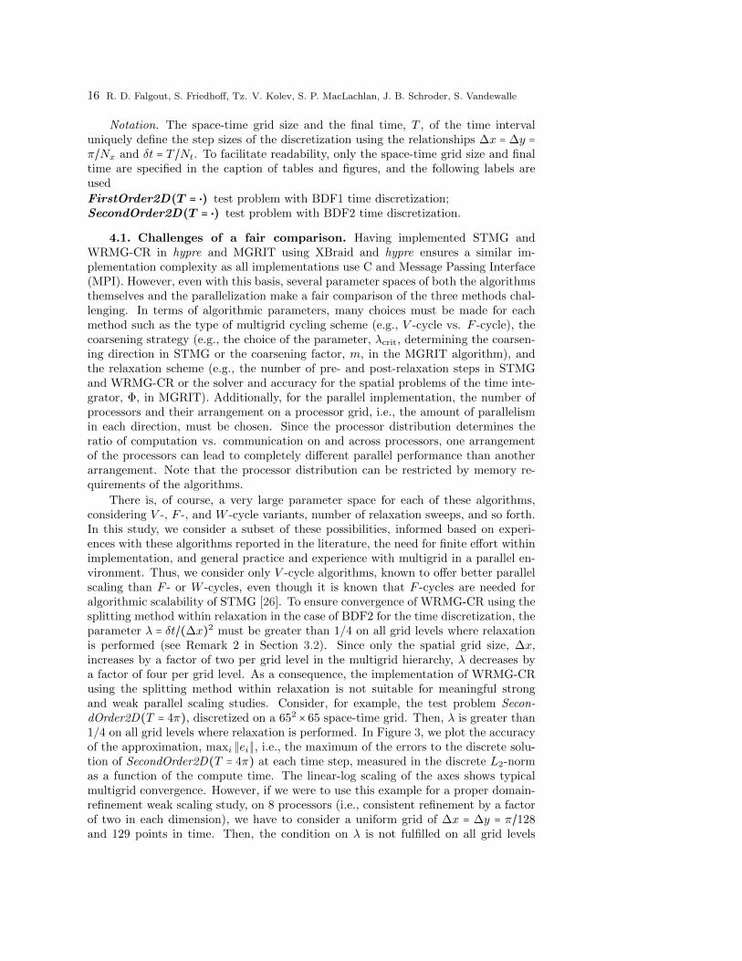
4.1. Challenges of a fair comparison. Having implemented STMG andWRMG-CR in hypre and MGRIT using XBraid and hypre ensures a similar im-plementation complexity as all implementations use C and Message Passing Interface(MPI). However, even with this basis, several parameter spaces of both the algorithmsthemselves and the parallelization make a fair comparison of the three methods chal-lenging. In terms of algorithmic parameters, many choices must be made for eachmethod such as the type of multigrid cycling scheme (e.g., V -cycle vs. F -cycle), thecoarsening strategy (e.g., the choice of the parameter, λcrit, determining the coarsen-ing direction in STMG or the coarsening factor, m, in the MGRIT algorithm), andthe relaxation scheme (e.g., the number of pre- and post-relaxation steps in STMGand WRMG-CR or the solver and accuracy for the spatial problems of the time inte-grator, Φ, in MGRIT). Additionally, for the parallel implementation, the number ofprocessors and their arrangement on a processor grid, i.e., the amount of parallelismin each direction, must be chosen. Since the processor distribution determines theratio of computation vs. communication on and across processors, one arrangementof the processors can lead to completely different parallel performance than anotherarrangement. Note that the processor distribution can be restricted by memory re-quirements of the algorithms.
There is, of course, a very large parameter space for each of these algorithms,considering V -, F -, and W -cycle variants, number of relaxation sweeps, and so forth.In this study, we consider a subset of these possibilities, informed based on experi-ences with these algorithms reported in the literature, the need for finite effort withinimplementation, and general practice and experience with multigrid in a parallel en-vironment. Thus, we consider only V -cycle algorithms, known to offer better parallelscaling than F - or W -cycles, even though it is known that F -cycles are needed foralgorithmic scalability of STMG [26]. To ensure convergence of WRMG-CR using thesplitting method within relaxation in the case of BDF2 for the time discretization, theparameter λ = δt/(∆x)2 must be greater than 1/4 on all grid levels where relaxationis performed (see Remark 2 in Section 3.2). Since only the spatial grid size, ∆x,increases by a factor of two per grid level in the multigrid hierarchy, λ decreases bya factor of four per grid level. As a consequence, the implementation of WRMG-CRusing the splitting method within relaxation is not suitable for meaningful strongand weak parallel scaling studies. Consider, for example, the test problem Secon-dOrder2D(T = 4π), discretized on a 652 × 65 space-time grid. Then, λ is greater than1/4 on all grid levels where relaxation is performed. In Figure 3, we plot the accuracyof the approximation, maxi ∥ei∥, i.e., the maximum of the errors to the discrete solu-tion of SecondOrder2D(T = 4π) at each time step, measured in the discrete L2-normas a function of the compute time. The linear-log scaling of the axes shows typicalmultigrid convergence. However, if we were to use this example for a proper domain-refinement weak scaling study, on 8 processors (i.e., consistent refinement by a factorof two in each dimension), we have to consider a uniform grid of ∆x = ∆y = π/128and 129 points in time. Then, the condition on λ is not fulfilled on all grid levels

Multigrid methods with space-time concurrency 17
in the multigrid hierarchy where relaxation is performed and, thus, one iteration ofthe splitting method within relaxation is not sufficient for convergence. Instead, forV (1,1)-cycles for example, we need 30 iterations of the splitting method to get rea-sonable convergence, which is prohibitively costly. For the BDF2 time discretization,we therefore do not include WRMG-CR in weak and strong parallel scaling studies.
0.5 1 1.5 2 2.5 3 3.510
−10
10−8
10−6
10−4
10−2
100
102
time [seconds]
ma
xim
um
err
or
WRMG−CR V(1,1)WRMG−CR V(2,1)
Fig. 3: Accuracy of the approximation to the solution of SecondOrder2D(T = 4π) ona 652 × 65 space-time grid using WRMG-CR V (1,1)- and V (2,1)-cycles and usingone iteration of the splitting method within relaxation on a single processor; each and represents one iteration of the V (1,1)- or V (2,1)-scheme, respectively.
4.2. Weak parallel scaling. We apply several variants of the three multigridschemes to the test problem. For both time discretization schemes, we look at compu-tation time and iteration counts to demonstrate good parallel scaling. In Section 4.3,this set of variants is then considered for the comparison to sequential time stepping.
Figure 4 shows weak parallel scaling results for several multigrid variants ap-plied to the test problem with BDF1 time discretization on the space-time domain[0, π]2 × [0, π2/64]. The problem size per processor is fixed at (roughly) 129 points ineach spatial direction and 257 points in the temporal direction. For proper domain-refinement, we quadruple the number of points in time when doubling the number ofpoints in space. Thus, on one processor, we use a uniform grid of ∆x = ∆y = π/128and 257 points in time while, on 4096 processors, we use a uniform grid of ∆x = ∆y =π/1024 and 16,385 points in time. Shown are results for STMG and WRMG-CRvariants with one pre- and one post-smoothing step and with two pre- and one post-smoothing step. The parameter λcrit determining the coarsening direction in STMGis chosen to be λcrit = 0.6 based on the Fourier analysis results in [26]. For MGRIT,we consider standard FCF -relaxation and a non-uniform coarsening strategy in thetemporal direction that coarsens by factors of 16 until fewer than 16 temporal pointsare left on each processor, then coarsens by factors of 2; details of the benefits ofthis coarsening strategy are described in [11]. Furthermore, we limit computationalwork of the spatial solves by limiting the number of PFMG iterations on the finegrid to a maximum of 9 iterations and to a maximum of 2 iterations on coarse grids.Additionally, we consider MGRIT with spatial coarsening, denoted MGRIT w/ sc. inthe figure, with space-coarsening using standard bilinear interpolation and restrictionoperators performed on grid levels with CFL-number δt/(∆x)2 > 2. The time curvesin Figure 4 show good parallel scaling for all three multigrid methods. More precisely,the overall compute time of both STMG variants and MGRIT with spatial coarseningincreases by a factor of about 1.3 over 4096-way parallelism, by a factor of about 1.6
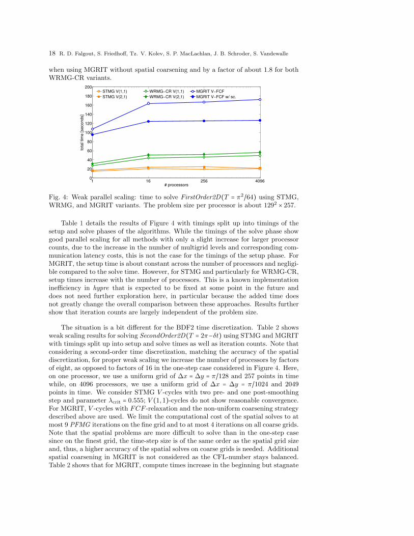
18 R. D. Falgout, S. Friedhoff, Tz. V. Kolev, S. P. MacLachlan, J. B. Schroder, S. Vandewalle
when using MGRIT without spatial coarsening and by a factor of about 1.8 for bothWRMG-CR variants.
1 16 256 40960
20
40
60
80
100
120
140
160
180
200
# processors
tota
l tim
e [
se
co
nd
s]
STMG V(1,1)
STMG V(2,1)
WRMG−CR V(1,1)
WRMG−CR V(2,1)
MGRIT V−FCF
MGRIT V−FCF w/ sc.
Fig. 4: Weak parallel scaling: time to solve FirstOrder2D(T = π2/64) using STMG,WRMG, and MGRIT variants. The problem size per processor is about 1292 × 257.
Table 1 details the results of Figure 4 with timings split up into timings of thesetup and solve phases of the algorithms. While the timings of the solve phase showgood parallel scaling for all methods with only a slight increase for larger processorcounts, due to the increase in the number of multigrid levels and corresponding com-munication latency costs, this is not the case for the timings of the setup phase. ForMGRIT, the setup time is about constant across the number of processors and negligi-ble compared to the solve time. However, for STMG and particularly for WRMG-CR,setup times increase with the number of processors. This is a known implementationinefficiency in hypre that is expected to be fixed at some point in the future anddoes not need further exploration here, in particular because the added time doesnot greatly change the overall comparison between these approaches. Results furthershow that iteration counts are largely independent of the problem size.
The situation is a bit different for the BDF2 time discretization. Table 2 showsweak scaling results for solving SecondOrder2D(T = 2π−δt) using STMG and MGRITwith timings split up into setup and solve times as well as iteration counts. Note thatconsidering a second-order time discretization, matching the accuracy of the spatialdiscretization, for proper weak scaling we increase the number of processors by factorsof eight, as opposed to factors of 16 in the one-step case considered in Figure 4. Here,on one processor, we use a uniform grid of ∆x = ∆y = π/128 and 257 points in timewhile, on 4096 processors, we use a uniform grid of ∆x = ∆y = π/1024 and 2049points in time. We consider STMG V -cycles with two pre- and one post-smoothingstep and parameter λcrit = 0.555; V (1,1)-cycles do not show reasonable convergence.For MGRIT, V -cycles with FCF -relaxation and the non-uniform coarsening strategydescribed above are used. We limit the computational cost of the spatial solves to atmost 9 PFMG iterations on the fine grid and to at most 4 iterations on all coarse grids.Note that the spatial problems are more difficult to solve than in the one-step casesince on the finest grid, the time-step size is of the same order as the spatial grid sizeand, thus, a higher accuracy of the spatial solves on coarse grids is needed. Additionalspatial coarsening in MGRIT is not considered as the CFL-number stays balanced.Table 2 shows that for MGRIT, compute times increase in the beginning but stagnate

Multigrid methods with space-time concurrency 19
number of processors, P = 1 16 256 4096
STMG 0.63 s 2.17 s 2.95 s 3.21 s
Tsetup WRMG-CR 2.13 s 4.59 s 6.17 s 7.78s
MGRIT 0.13 s 0.14 s 0.14 s 0.14 s
STMG V (1,1) 14.42 s 18.75 s 16.64 s 17.06 s
STMG V (2,1) 16.06 s 21.06 s 21.66 s 18.83 s
WRMG-CR V (1,1) 25.13 s 39.51 s 39.44 s 41.53 s
Tsolve WRMG-CR V (2,1) 29.08 s 46.13 s 45.75 s 48.36 s
MGRIT 107.21 s 163.78 s 167.10 s 171.97 s
MGRIT w/ sc. 94.82 s 124.33 s 125.09 s 126.71 s
STMG V (1,1) 7 7 6 7
STMG V (2,1) 6 6 6 5
WRMG-CR V (1,1) 5 5 5 5
iter WRMG-CR V (2,1) 4 4 4 4
MGRIT 5 6 6 6
MGRIT w/ sc. 5 5 5 5
Table 1: Weak parallel scaling: setup and solve times and number of iterations forsolving FirstOrder2D(T = π2/64) using STMG, WRMG, and MGRIT variants. Theproblem size per processor is about 1292 × 257.
at higher processor counts. Although stagnation is observed at larger processor countsthan in the one-step case, the overall compute time increases by a factor of about 1.6(the same as in the one-step case) over 4096-way parallelism. Furthermore, Table 2shows that iteration counts are again independent of the problem size.
number of processors, P = 1 8 64 512 4096
Tsetup STMG 0.57 s 1.92 s 3.71 s 4.17 s 4.53 s
MGRIT 0.13 s 0.14 s 0.14 s 0.14 s 0.14 s
Tsolve STMG V (2,1) 33.66 s 42.00 s 62.52 s 63.08 s 76.90 s
MGRIT 162.17 s 209.29 s 236.31 s 250.35 s 261.49 s
iter STMG V (2,1) 14 16 19 19 23
MGRIT 4 4 4 4 4
Table 2: Weak parallel scaling: setup and solve times and number of iterations forsolving SecondOrder2D(T = 2π− δt) using STMG and MGRIT. The problem size perprocessor is about 1292 × 257.
For the STMG method, however, compute times increase by a factor of about 2.4over 4096-way parallelism and iteration counts do not appear to be perfectly boundedindependently of the problem size. The increase in iteration counts indicates thatthe implementation is not robust with respect to the discretization grid which isconsistent with results in [26]. For a robust implementation, F -cycles have to beconsidered; however, this implementation effort would go beyond the scope of thispaper and the factor of 1.5 in iterations with V -cycles almost certainly outweighs theworse parallel scalability expected to be seen with F -cycles.
4.3. Strong parallel scaling. The above results show that the three multigridmethods obtain good weak parallel scalability, particularly for the BDF1 time dis-cretization. Now, we focus on the performance of these methods compared with oneanother and to traditional space-parallel algorithms with sequential time stepping.
Figure 5 shows compute times for solving FirstOrder2D(T = π2) on a 1282×16,384space-time grid using the set of STMG, WRMG-CR, and MGRIT variants consid-ered in the weak parallel scaling study in Figure 4 and a space-parallel algorithm

20 R. D. Falgout, S. Friedhoff, Tz. V. Kolev, S. P. MacLachlan, J. B. Schroder, S. Vandewalle
with sequential time stepping. For the time-stepping approach, the spatial domainis distributed evenly such that each processor’s subdomain is approximately a squarein space. When using 16 processors, for example, each processor owns a square ofapproximately 32 × 32. Since considering 16 processors for distributing the spatialdomain appears to be an efficient use of computational resources with respect to ben-efits in runtime, for the space-time approaches, we parallelize over 16 processors in thespatial dimensions, with increasing numbers of processors in the temporal dimension.That is, with Pt denoting the number of processors used for temporal parallelism,the space-time domain is distributed across 16Pt processors such that each processorowns a space-time hypercube of approximately 322 × 16,384/Pt. Note that due to thestorage requirements of STMG and WRMG-CR, at least eight processors for temporalparallelism must be used in order to avoid memory issues in the given parallel com-putational environment. For MGRIT, even Pt = 1 would be possible, but the requiredcompute time is much larger than for any of the other methods, due to the computa-tional overhead inherent in the MGRIT approach; thus, Figure 5 only presents resultsfor MGRIT with Pt ≥ 4. Results demonstrate the large computational overhead of theMGRIT approach in contrast with STMG, WRMG-CR, and traditional time step-ping. However, this extra work can be effectively parallelized at very large scales withexcellent strong parallel scalability. While on smaller numbers of processors, MGRITis slower than time stepping we see good speedup at higher processor counts. Forexample, considering 64 processors, the space-parallel algorithm with sequential timestepping is faster than the space-time-concurrent MGRIT algorithm by a factor ofabout six or by a factor of about four when considering MGRIT with spatial coarsen-ing. Increasing the number of processors to 16,384, however, MGRIT is faster with aspeedup of up to a factor of about 42 compared to sequential time stepping with 16processors used for spatial parallelism.
1 4 16 64 256 1024 4096 16,38410
−2
100
102
104
# processors
tim
e [
se
co
nd
s]
STMG V(1,1)STMG V(2,1)WRMG−CR V(1,1)WRMG−CR V(2,1)MGRIT V−FCFMGRIT V−FCF w/ sc.time stepping
Fig. 5: Strong parallel scaling: time to solve FirstOrder2D(T = π2) on a 1282×16,384space-time grid using sequential time-stepping, STMG, WRMG-CR, and MGRIT.
With STMG and WRMG-CR, we can benefit over the time stepping approachat much smaller scales and achieve greater speedup at high processor counts. Con-sidering 128 processors, i.e., adding eight-way temporal parallelism to 16-way spatialparallelism, STMG is already faster than 16-way space-parallel time stepping, witha speedup of up to a factor of about 15. For WRMG-CR, the speedup is about afactor of five. Increasing the number of processors to 16,384 results in a speedup,measured relative to the time for time stepping with 16-way spatial parallelism, of

Multigrid methods with space-time concurrency 21
up to a factor of 82 for WRMG-CR and of 723 for STMG. Scaling properties of thetwo approaches are excellent at the beginning, with poorer scaling at larger processorcounts, especially for the WRMG-CR method. For higher levels of temporal paral-lelism, the number of time steps per processor is small and cyclic reduction becomesproblematic which can be explained by the performance models developed in Section3.4, as will be discussed in Section 4.4.
Figure 6 details “effective” parallel efficiencies, i.e., parallel efficiencies relative tosequential time stepping on a single processor, for one variant of each time-integrationapproach considered in Figure 5. For STMG, the numbers are very steady out to 2048cores, and then despite modest degradation, are still better than the other methods outto 16K processors. For WRMG-CR, the numbers are less steady, but still acceptablerelative to time-stepping. For MGRIT, the effective efficiencies are small, but almostperfectly steady out to 16K cores, demonstrating its excellent strong scaling.
1 4 16 64 256 1024 4096 16,3840.01
0.1
1
10
100
# processors
eff
icie
ncy [
%]
STMG V(1,1)WRMG−CR V(2,1)MGRIT V−FCF w/ sc.time stepping
Fig. 6: Strong scaling efficiencies of sequential time-stepping, STMG, WRMG-CR,and MGRIT. For each method, parallel efficiency is measured relative to time steppingon a single processor as T (1)/(P ⋅ T (P )) ⋅ 100, where T (P ) is the wall-clock timerequired for solution on P processors.
In the case of the BDF2 time discretization, compute times have very similarqualitative properties. Figure 7 shows compute times of a space-parallel algorithmwith sequential time stepping, as well as the STMG and MGRIT variants consideredin Figure 4 applied to SecondOrder2D(T = 4π − π/512) on a space-time grid of size5132×4096. Here, for STMG and MGRIT, we consider adding temporal parallelism totwo different levels of spatial parallelism, i.e., we look at using 64 and 256 processorsfor distributing the spatial domain. If we denote the number of processors used fortemporal parallelism in the two multigrid schemes by Pt, when using 64-way paral-lelism in space, the space-time domain is distributed across 64Pt processors such thateach processor owns a space-time hypercube of approximately 642 × 4096/Pt. Analo-gously, considering 256-way parallelism in space, the space-time domain is distributedacross 256Pt processors such that each processor owns a space-time hypercube of ap-proximately 322 × 4096/Pt. The time curves show that the crossover point for whichit becomes beneficial to use MGRIT for this particular problem and the speedupcompared to time stepping at large processor counts depends on the levels of spatialand temporal parallelism. More precisely, for this particular problem, for MGRITto break even with sequential time stepping using a fixed level of spatial parallelism,we need to add about 16-way parallelism in time. For 64-way parallelism in space,for example, we need about 1024 processors for MGRIT to break even with sequen-

22 R. D. Falgout, S. Friedhoff, Tz. V. Kolev, S. P. MacLachlan, J. B. Schroder, S. Vandewalle
tial time stepping. Increasing the number of processors to 8192 results in a speedupof a factor of seven compared to sequential time stepping with 64-way parallelism.A similar comparison can be made for 256-way parallelism in space. Note that forMGRIT with 64-way parallelism in space and 8192 processors in total, the number oftime-step pairs per processors is 16 corresponding to the coarsening factor and, thus,further increasing the number of processors is not beneficial.
16 64 256 512 1024 2048 4096 8192 16,384
2
5
10
25
50
90
160
300410
# processors
tim
e [secon
ds]
STMG V(2,1) (64 procs in space)STMG V(2,1) (256 procs in space)MGRIT V−FCF (64 procs in space)MGRIT V−FCF (256 procs in space)time stepping
Fig. 7: Strong parallel scaling: time to solve SecondOrder2D(T = 4π − π/512) on a5132 × 4,096 space-time grid using sequential time-stepping, STMG, and MGRIT.
The dependency of compute times on the levels of spatial and temporal parallelismis not as pronounced in the STMG approach as in the MGRIT approach. Whilefor smaller numbers of processors it is slightly beneficial to use fewer processors forspatial parallelism, on larger processor counts compute times of both variants are verysimilar. Comparing to the space-parallel algorithm with sequential time stepping, themaximum speedup of STMG is about a factor of 15 larger than that of MGRIT.
Figure 8 details “effective” parallel efficiencies, i.e., parallel efficiencies relativeto sequential time stepping on a single processor, for the time-integration approachesconsidered in Figure 7. For both STMG and MGRIT, numbers are about steady outto large processor counts. Comparing the two multigrid approaches, the difference ineffective parallel efficiencies diminishes when going from the BDF1 to the BDF2 timediscretization. More precisely, while in Figure 6, efficiencies for STMG are between15 and 40% and for MGRIT about 1%, in Figure 8, efficiencies for STMG are between11 and 16% and for MGRIT between 1 and 3%.
4.4. Insights from the parallel models. The above results demonstrate thatthe two intrusive approaches show somewhat poorer parallel scalability than theMGRIT algorithm. To better understand the parallel scalability, we use the mod-els developed in Section 3.4. Based on data in [15, Table 2], we choose the set ofmachine parameters given by
(4.1) α = 1 µs, β = 0.74 ns/double, γ = 0.15 ns/flop,
characterizing a modern communication-dominant machine. To define the parameterset, we have set α = 1 µs and chosen β and γ such that the ratios α/β and α/γare equal to the maximum ratios from [15, Table 2]. Figure 9 shows predicted timesto solve FirstOrder2D(T = π2) on a 1282 × 16,384 space-time grid using sequentialtime stepping, STMG, WRMG-CR, and MGRIT. The parameters in the models arechosen as in the strong parallel scaling study in Figure 5. Note that for STMG, models

Multigrid methods with space-time concurrency 23
1 4 16 64 256 1024 4096 16,3840.1
1
10
100
# processors
effic
iency [%
]
STMG V(2,1) (64 procs in space)STMG V(2,1) (256 procs in space)MGRIT V−FCF (64 procs in space)MGRIT V−FCF (256 procs in space)time stepping
Fig. 8: Strong scaling efficiencies of sequential time-stepping, STMG, and MGRIT.For each method, parallel efficiency is measured relative to time stepping on a singleprocessor as T (1)/(P ⋅ T (P )) ⋅ 100, where T (P ) is the wall-clock time required forsolution on P processors.
for the extreme cases of coarsening only in space and of coarsening only in time areused. Results show that predicted time curves behave qualitatively very similar toexperimentally measured runtimes depicted in Figure 5.
1 4 16 64 256 1024 4096 16,38410
−4
10−2
100
102
104
# processors
tim
e [
se
co
nd
s]
STMG V(1,1) (x−coarsening)STMG V(1,1) (t−coarsening)WRMG−CR V(1,1)MGRIT V−FCFtime stepping
Fig. 9: Predicted times to solve FirstOrder2D(T = π2) on a 1282 × 16,384 space-timegrid using sequential time-stepping, STMG, WRMG-CR, and MGRIT.
The models also explain the somewhat poorer parallel scalability of STMG andWRMG-CR at higher processor counts in this specific parallel scaling study. ForWRMG-CR, cyclic reduction becomes problematic introducing an additional loga-rithmic factor in the communication cost. More precisely, assuming that the space-time grid of size N2
x ×Nt is distributed evenly such that each processor’s subdomainis approximately of size n2
x × nt, the β-term in the WRMG-CR-model of νWRMG
V (ν1, ν2)-cycles is given by
T(WRMG)β ≈ νWRMG [8(ν1 + ν2 + (5/2))nxnt + (4/3)((2 log2(Nt) + 1)(ν1 + ν2) + 1)n2
x]β.If we fix nx as in the strong scaling study of the numerical experiment, the secondterm is constant and becomes dominant as nt decreases. Thus, we expect poorerscalability when
nt <((2 log2(Nt) + 1)(ν1 + ν2) + 1)
8 (ν1 + ν2 + (5/2)) nx.

24 R. D. Falgout, S. Friedhoff, Tz. V. Kolev, S. P. MacLachlan, J. B. Schroder, S. Vandewalle
For the problem considered in Figures 5 and 9 and one pre- and one postrelaxationsweep within WRMG-CR, the β-term causes loss in parallel scalability for nt < 2.19nx,which is the case for about 4096 processors and higher processor counts. The loss inparallel scalability for STMG at higher numbers of processors when fixing nx canbe similarly explained by considering the β-term in the STMG model with temporalsemicoarsening.
Having validated the models with experimental data, we now use the models forestimating the parallel scalability of the four time integration approaches on modernlarge-scale machines. In the models, we assume a communication-dominant environ-ment with machine parameters given in (4.1). We consider a domain refinement ofthe problem in Figures 5 and 9, i.e., we consider solving FirstOrder2D(T = π2) on aspace-time grid of size 10242 × 131,072 instead of on a 1282 × 16,384 space-time grid.Analogously to the numerical experiment, for the space-parallel algorithm with se-quential time stepping, we assume that the spatial domain is evenly distributed suchthat each processor holds approximately a square in space. For the space-parallelmultigrid approaches, we add temporal parallelism to 64-way spatial parallelism, as64 processors are effectively utilized in the time-stepping approach.
Figure 10 shows expected parallel scaling for solving FirstOrder2D(T = π2) ona 10242 × 131,072 space-time grid using the four time-integration approaches. Themodels indicate a similar scaling behavior on large numbers of processors as seenin numerical experiments at small scale. We note that the expected good parallelscalability of the three space-time-concurrent multigrid approaches partially relies onthe assumption of large communication-to-computation ratios on modern large-scalecomputers.
1 4 16 64 256 1024 4096 16,384 131,072 1,048,576
10−2
100
102
104
# processors
tim
e [
se
co
nd
s]
STMG V(1,1) (x−coarsening)STMG V(1,1) (t−coarsening)WRMG−CR V(1,1)MGRIT V−FCFtime stepping
Fig. 10: Predicted times to solve FirstOrder2D(T = π2) on a 10242 × 131,072 space-time grid using sequential time-stepping, STMG, WRMG-CR, and MGRIT.
4.5. Potential improvements to XBraid. The purpose of this paper is tocompare WRMG, STMG and MGRIT, as implemented in their “pure” forms, i.e., tocompare the three parallel-in-time strategies that (1) only semicoarsen in space, (2)only semicoarsen in time and (3) coarsen in both space and time. Not surprisingly,the most efficient solution is to coarsen in both space and time (STMG). The slowest(at least for many problem sizes) is to coarsen only in time (MGRIT).
To address this, current research in the XBraid project is considering approachesfor incorporating aspects of STMG into XBraid. This will allow XBraid to be moreintrusive, but to also achieve efficiencies closer to those of STMG. The ultimate goalis to allow the user to choose the level of intrusiveness that his/her application can
Multigrid methods with space-time concurrency 25
tolerate, and to enjoy the maximum benefit of time parallelism for that application.In other words, the more intrusive the chosen parallel-in-time implementation, thebetter the potential speedup.
One such improvement is faster residual computations. The computation of theresidual from (2.6) requires a matrix inversion for the application of Φδt at every timepoint. In other words, the computation of the residual is as expensive (in terms ofFLOPS) as the entire traditional time-stepping approach. The alternative used bySTMG is to form the residual based on the matrix stencil [−I Φ−1
δt ] rather than theMGRIT stencil [−Φδt I]. Note that here the matrix Φ−1
δt is sparse and relativelycheap to evaluate, and as such, this alternate residual has the potential to save sig-nificant compute and messaging time. Taking the largest test case for P = 4096 fromTable 1, for example, the time spent computing residuals in MGRIT is 21 seconds outof the total time of 172 seconds. This change would largely eliminate this cost.
Another example improvement is to allow for variable storage in XBraid. Allowingfor storage at every time point allows for user-implemented point-wise relaxation,as in STMG. Current F (CF )-relaxation involves expensive matrix inversions andtherefore, cheap point-wise relaxation could offer similar speedups as those availablefrom faster residual computations. Lastly, full storage of every time point would allowfor improved initial guesses to the (non)linear solvers called by implicit methods.
5. Conclusion. Current trends in computer architectures leading towards sys-tems with more, but not faster processors, induce a change in the development ofalgorithms for evolutionary problems. Instead of exploiting increasing clock speeds,faster time-to-solution must come from increasing concurrency, driving the develop-ment of algorithms with space-time concurrency. Motivated by this development, thecomparison of three multigrid methods with space-time concurrency, STMG, WRMG-CR, and MGRIT, is considered.
Parallel results show that all three multigrid methods with space-time concurrencyconsidered in this paper are effective solvers for diffusion problems. In the case wheremany more processors are available than can be effectively utilized by sequential time-stepping, performance of all three multigrid methods with space-time concurrencyis better than that of space-parallel time stepping. The speedup in comparison tosequential time stepping is larger for the invasive STMG and WRMG-CR approachesthan for the non-invasive MGRIT approach. However, the two intrusive approachesshow somewhat poorer parallel scalability than the MGRIT algorithm.
Balancing MGRIT’s less efficient approach are some key practical advantages.While the generalization to problems in three space dimensions is straightforwardwith the non-intrusive MGRIT approach, the effort for a parallel implementationof the two intrusive approaches STMG and WRMG-CR is immense. Furthermore,MGRIT allows for memory savings equal to the coarsening factor (here 16x), whichis another appealing advantage over the two invasive approaches1.
Extending the comparison presented in this paper to include other time-dependentproblems is exceedingly difficult, due to the intrusiveness of STMG and WRMG-CR.Although benefits in runtime are likely much smaller with the MGRIT approach,its non-intrusiveness easily allows effective exploitation of substantially more compu-tational resources than with space-parallel time stepping. More concretely, since
1One possibility to save on memory in the waveform relaxation approach is to subdivide thetime interval into a sequence of “windows” that are treated sequentially [44]. However, there is anapparent parallel performance tradeoff with this reduction in storage requirement.

26 R. D. Falgout, S. Friedhoff, Tz. V. Kolev, S. P. MacLachlan, J. B. Schroder, S. Vandewalle
MGRIT uses the same time-integration operator as algorithms based on a time-stepping approach, problem-specific time-integration operators are handled naturally.On the other hand, it is not clear how to extend STMG and WRMG-CR to other prob-lem types in cases where specific time-integration schemes are crucial for convergenceof time stepping.
REFERENCES
[1] hypre: High performance preconditioners. http://www.llnl.gov/CASC/hypre/.[2] XBraid: Parallel multigrid in time. http://llnl.gov/casc/xbraid.[3] S. F. Ashby and R. D. Falgout, A parallel multigrid preconditioned conjugate gradient al-
gorithm for groundwater flow simulations, Nuclear Science and Engineering, 124 (1996),pp. 145–159. UCRL-JC-122359.
[4] P. Bastian, J. Burmeister, and G. Horton, Implementation of a parallel multigrid methodfor parabolic partial differential equations, in Parallel Algorithms for PDEs, Proc. 6thGAMM Seminar Kiel, January 19-21, 1990, W. Hackbusch, ed., Braunschweig, 1990,Vieweg Verlag, pp. 18–27.
[5] M. Bjørhus, On Domain Decomposition, Subdomain Iteration and Waveform Relaxation,PhD thesis, Department of Mathematical Sciences, Norwegian Institute of Technology,University of Trondheim, Trondheim, Norway, 1995.
[6] A. Brandt, Multi–level adaptive solutions to boundary–value problems, Math. Comp., 31(1977), pp. 333–390.
[7] B. L. Buzbee, G. H. Golub, and C. W. Nielson, On direct methods for solving Poisson’sequations, SIAM J. Numer. Anal., 7 (1970), pp. 627–656.
[8] P. Chartier and B. Philippe, A parallel shooting technique for solving dissipative ODEs,Computing, 51 (1993), pp. 209–236.
[9] A. J. Christlieb, C. B. Macdonald, and B. W. Ong, Parallel high-order integrators, SIAMJ. Sci. Comput., 32 (2010), pp. 818–835.
[10] M. Emmett and M. L. Minion, Toward an efficient parallel in time method for partial differ-ential equations, Commun. Appl. Math. Comput. Sci., 7 (2012), pp. 105–132.
[11] R. D. Falgout, S. Friedhoff, Tz. V. Kolev, S. P. MacLachlan, and J. B. Schroder,Parallel time integration with multigrid, SIAM Journal on Scientific Computing, 36 (2014),pp. C635–C661.
[12] R. D. Falgout and J. E. Jones, Multigrid on massively parallel architectures, in MultigridMethods VI, E. Dick, K. Riemslagh, and J. Vierendeels, eds., vol. 14 of Lecture Notesin Computational Science and Engineering, Springer-Verlag, 2000, pp. 101–107. Proc. ofthe Sixth European Multigrid Conference held in Gent, Belgium, September 27-30, 1999.UCRL-JC-133948.
[13] R. D. Falgout, A. Katz, Tz. V. Kolev, J. B. Schroder, A. Wissink, and U. M. Yang,Parallel time integration with multigrid reduction for a compressible fluid dynamics appli-cation, Journal of Computational Physics, (2014). Submitted.
[14] S. Friedhoff and S. MacLachlan, A generalized predictive analysis tool for multigrid meth-ods, Numerical Linear Algebra with Applications, 22 (2015), pp. 618–647.
[15] H. Gahvari, A. Baker, M. Schulz, U. Meier Yang, K. Jordan, and W. Gropp, Model-ing the Performance of an Algebraic Multigrid Cycle on HPC Platforms, in 25th ACMInternational Conference on Supercomputing, Tucson, AZ, 2011.
[16] M. J. Gander, 50 years of Time Parallel Time Integration, in Multiple Shooting and TimeDomain Decomposition, Springer, 2015. In press.
[17] M. J. Gander and M. Neumuller, Analysis of a new space-time parallel multigrid algorithmfor parabolic problems. arXiv:1411/0519, 2014.
[18] M. J. Gander and A. M. Stuart, Space-time continuous analysis of waveform relaxation forthe heat equation, SIAM Journal on Scientific Computing, 19 (1998), pp. 2014–2031.
[19] M. J. Gander and S. Vandewalle, Analysis of the parareal time-parallel time-integrationmethod, SIAM J. Sci. Comput., 29 (2007), pp. 556–578.
[20] S. Guttel, A parallel overlapping time-domain decomposition method for ODEs, in Domaindecomposition methods in science and engineering XX, vol. 91 of Lect. Notes Comput. Sci.Eng., Springer, Heidelberg, 2013, pp. 459–466.
[21] W. Hackbusch, Parabolic multigrid methods, in Computing methods in applied sciences andengineering, VI (Versailles, 1983), North-Holland, Amsterdam, 1984, pp. 189–197.
[22] R. W. Hockney, A fast direct solution of Poisson’s equation using Fourier analysis, J. Assoc.

Multigrid methods with space-time concurrency 27
Comput. Mach., 12 (1965), pp. 95–113.[23] R. W. Hockney and C. R. Jesshope, Parallel Computers: Architecture, Programming and
Algorithms, Adam Hilger, Bristol, 1981.[24] G. Horton, The time-parallel multigrid method, Comm. Appl. Numer. Methods, 8 (1992),
pp. 585–595.[25] G. Horton and R. Knirsch, A time-parallel multigrid-extrapolation method for parabolic
partial differential equations, Parallel Comput., 18 (1992), pp. 21–29.[26] G. Horton and S. Vandewalle, A space-time multigrid method for parabolic partial differ-
ential equations, SIAM J. Sci. Comput., 16 (1995), pp. 848–864.[27] G. Horton, S. Vandewalle, and P. Worley, An algorithm with polylog parallel complex-
ity for solving parabolic partial differential equations, SIAM J. Sci. Comput., 16 (1995),pp. 531–541.
[28] H. B. Keller, Numerical methods for two-point boundary-value problems, Blaisdell PublishingCo. Ginn and Co., Waltham, Mass.-Toronto, Ont.-London, 1968.
[29] P. M. Kogge and H. S. Stone, A parallel algorithm for the efficient solution of a generalclass of recurrence equations, IEEE Transactions on Computers, C-22 (1973), pp. 786–793.
[30] E. Lelarasmee, A. E. Ruehli, and A. L. Sangiovanni-Vincentelli, The waveform relaxationmethod for time-domain analysis of large scale integrated circuits, IEEE CAD, 1 (1982).
[31] J.-L. Lions, Y. Maday, and G. Turinici, Resolution d’EDP par un schema en temps“parareel”, C. R. Acad. Sci. Paris Ser. I Math., 332 (2001), pp. 661–668.
[32] C. Lubich and A. Ostermann, Multigrid dynamic iteration for parabolic equations, BIT, 27(1987), pp. 216–234.
[33] Y. Maday and E. M. Rønquist, Parallelization in time through tensor-product space-time solvers, Comptes Rendus Mathematique. Academie des Sciences. Paris, 346 (2008),pp. 113–118.
[34] M. L. Minion and S. A. Williams, Parareal and spectral deferred corrections, in NumericalAnalysis and Applied Mathematics, T. E. Simos, ed., no. 1048 in AIP Conference Proceed-ings, AIP, 2008, pp. 388–391.
[35] W. L. Miranker and W. Liniger, Parallel methods for the numerical integration of ordinarydifferential equations, Math. Comp., 21 (1967), pp. 303–320.
[36] J. Nievergelt, Parallel methods for integrating ordinary differential equations, Comm. ACM,7 (1964), pp. 731–733.
[37] M. Ries and U. Trottenberg, MGR-ein blitzschneller elliptischer Loser, Tech. ReportPreprint 277 SFB 72, Universitat Bonn, 1979.
[38] M. Ries, U. Trottenberg, and G. Winter, A note on MGR methods, J. Lin. Alg. Applic.,49 (1983), pp. 1–26.
[39] D. Sheen, I. H. Sloan, and V. Thomee, A parallel method for time discretization of parabolicequations based on Laplace transformation and quadrature, IMA Journal of NumericalAnalysis, 23 (2003), pp. 269–299.
[40] R. Speck, D. Ruprecht, M. Emmett, M. Bolten, and R. Krause, A space-time parallelsolver for the three-dimensional heat equation, in Parallel Computing: Accelerating Com-putational Science and Engineering (CSE), vol. 25 of Advances in Parallel Computing, IOSPress, 2014, pp. 263–272.
[41] H. De Sterck, T. A. Manteuffel, S. F. McCormick, and L. Olson, Least-squares finiteelement methods and algebraic multigrid solvers for linear hyperbolic PDEs, SIAM J. Sci.Comput., 26 (2004), pp. 31–54.
[42] S. Vandewalle and G. Horton, Fourier mode analysis of the multigrid waveform relaxationand time-parallel multigrid methods, Computing, 54 (1995), pp. 317–330.
[43] S. Vandewalle and R. Piessens, Efficient parallel algorithms for solving initial-boundaryvalue and time-periodic parabolic partial differential equations, SIAM J. Sci. Statist. Com-put., 13 (1992), pp. 1330–1346.
[44] S. G. Vandewalle and E. F. Van de Velde, Space-time concurrent multigrid waveform relax-ation, Ann. Numer. Math., 1 (1994), pp. 347–360. Scientific computation and differentialequations (Auckland, 1993).
[45] T. Weinzierl and T. Koppl, A geometric space-time multigrid algorithm for the heat equation,Numer. Math. Theory Methods Appl., 5 (2012), pp. 110–130.