Embed Size (px)
Citation preview
ALGEBRAIC MULTIGRID DOMAIN AND RANGEDECOMPOSITION (AMG-DD/AMG-RD)∗
R. BANK†, R. D. FALGOUT‡, T. JONES §,T. A. MANTEUFFEL§, S. F. MCCORMICK§, J. W.
RUGE§
Abstract.
In modern large-scale supercomputing applications, Algebraic MultiGrid (AMG) is a leadingchoice for solving matrix equations. However, the high cost of communication relative to that ofcomputation is a concern for the scalability of traditional implementations of AMG on emergingarchitectures. This paper introduces two new algebraic multilevel algorithms, Algebraic MultiGridDomain Decomposition (AMG-DD) and Algebraic MultiGrid Range Decomposition (AMG-RD),that replace traditional AMG V-cycles with a fully overlapping domain decomposition approach.While the methods introduced here are similar in spirit to the geometric methods developed byBrandt and Diskin [1], Mitchell [2], and Bank and Holst [3], they differ primarily in that they arepurely algebraic: AMG-RD and AMG-DD trade communication for computation by forming globalcomposite “grids” based only on the matrix, not the geometry. (As is the usual AMG convention,“grids” here should only be taken in the algebraic sense, regardless of whether or not it correspondsto any geometry.) Another important distinguishing feature of AMG-RD and AMG-DD is theirnovel residual communication process that enables effective parallel computation on composite grids,avoiding the all-to-all communication costs of the geometric methods. The main purpose of thispaper is to study the potential of these two algebraic methods as possible alternatives to existingAMG approaches for future parallel machines. To this end, this paper develops some theoreticalproperties of these methods and reports on serial numerical tests of their convergence properties overa spectrum of problem parameters.
Key words. iterative methods, multigrid, algebraic multigrid, parallel, scalability, domaindecomposition
1. Introduction. Multigrid methods are often well-suited for large-scale scien-tific computing problems because they offer the possibility of an O(N) method forsolving equations of the form A0u0 = f0, where A0 is an N ×N matrix. However, thechallenge for multigrid and other matrix equation solvers on large parallel machinesis that performance can suffer from the high cost of communication relative to that ofcomputation. While Algebraic MultiGrid (AMG [4, 5]) solvers scale nearly optimally,they too are increasingly affected by relative communication costs as the numberof processors increase. Indeed, all known parallel multigrid algorithms experienceO(log(N)) communication costs for the main computation in each V-Cycle. Previousgeometric multilevel approaches developed by [1, 2, 6, 3, 7, 8, 9, 10, 11] aimed to re-duce the constant in this O(log(N)) cost by trading communication for computationusing redundant processing on overlapping grids. Inspired by these efforts, the Alge-braic MultiGrid Domain (AMG-DD) and Range Decomposition (AMG-RD) methodsintroduced here attempt to achieve the same goal by tasking possibly otherwise idleprocessors to perform redundant computations via a domain decomposition approach;
∗Submitted to SIAM Journal of Scientific Computing, June 30, 2014. This work was performedunder the auspices of the U.S. Department of Energy by Lawrence Livermore National Laboratoryunder Contract DE-AC52-07NA27344 (LLNL-JRNL-666751).†Department of Mathematics, University of California at San Diego, La Jolla, CA 92093. email:
[email protected]‡Center for Applied Scientific Computing, Lawrence Livermore National Laboratory, P.O. Box
808, L-561, Livermore, CA 94551. email: [email protected]§Department of Applied Mathematics, University of Colorado at Boulder, Boulder, CO
80309–0526 email: [email protected], [email protected], [email protected],[email protected]
1

the basic idea is to use subdomains that fully overlap at coarse scales. Our departurefrom the previous geometric approaches is to exploit the benefits of domain decomposi-tion in a purely algebraic AMG setting. AMG-DD and AMG-RD first assume that thesetup for an effective AMG implementation has been formed [4, 5]. The two methodsthen use the global AMG hierarchical constructs (coarse grids, coarse-grid operators,and intergrid transfer operators) to create a composite grid for each processor. (Ouruse of geometric terms such as “grid” and “domain” should be taken in an algebraicsense, as is common in the AMG literature. While these objects may in many caseshave an underlying geometry, we make no such assumptions here. No aspects of themethods that we discuss use any notion of, or depend upon, an underlying geometry–the constructs are all purely algebraic. Nevertheless, we use the geometric conventionhere because it makes for a clearer discussion.) Each composite grid consists of theoriginal grid in and about the subdomain owned by its associated processor and ofgrids that are increasingly coarse as they extend away from the processor subdomainto the boundary. These composite grids are formed algebraically and directly from thehierarchical constructs determined in the traditional AMG setup phase. In this way,AMG-DD and AMG-RD can be thought of as globally overlapping domain decompo-sition methods that have reduced communication per cycle, since they do not requirecommunication on each grid level as standard AMG methods do. Moreover, the newprocess introduced here provides an efficient communication phase between each cy-cle, in contrast to the expensive all-to-all communication processes of the previousgeometric approaches. The composite grids thus provide a means for maintainingeffective communication between processors that controls cost and maintains optimalconvergence rates.
The main focus of this paper is to study the potential of these AMG-DD andAMG-RD as possible alternatives to existing AMG approaches for solving large-scalematrix equations on advanced parallel machines. To this end, this paper developssome theoretical properties of these methods and reports on serial numerical tests oftheir convergence properties over a spectrum of parameters on a model problem. Alsoincluded are some heuristics and a parameter study based on a performance model,both of which are designed to anticipate the potential of AMG-DD and AMG-RD foruse on emerging parallel architectures.
Since AMG-DD and AMG-RD are constructed on top of an existing AMG hi-erarchy, the cost of the setup, as in all AMG algorithms, needs to be addressed. Ina purely serial setting, setup costs for AMG-DD and AMG-RD can be up to abouttwice that of standard AMG due to the redundant calculation that we use. How-ever, in parallel, owing to the construction of the algorithm from existing operators,the increased setup cost can be reduced essentially to the cost of communicating thecomponents of the operators needed to each processor. This communication can bedone using the same pattern as the residual communication and, as such, is boundedin cost by that of performing one extra V-Cycle.
We begin by outlining a traditional AMG implementation and setup, and thenspecifying how AMG-DD and AMG-RD are constructed. While a wide range ofparameters can be used to create the solvers, in the interest of space, we explore justa few choices and how they affect convergence and scalability of the algorithms. Weshow here that AMG-DD and AMG-RD are algebraic duals of each other in the energyinner product, and we establish convergence of these methods in a two-level setting.(This paper focuses mainly on AMG-DD, but AMG-RD is included because it maybe more convenient for some applications and because the two methods together can
2

be used in sequence to provide a self-adjoint scheme.)To provide a framework for building models and estimates for scalability, the re-
sults in this paper are restricted to determining the effects of the algorithms on themodel 2D Poisson equation. We present several numerical results from which we canform models of how parallel AMG and AMG-DD are expected to scale. These resultssuggest that, for current parallel architectures, the trading of communication for com-putation that AMG-DD achieves puts it essentially at break even with AMG in termsof parallel efficiency. This parity comes perhaps more from the remarkable parallelefficiency of advanced AMG solvers [12] than any lack of efficiency of the methods de-veloped here. Nevertheless, in addition to their fault tolerance advantages that resultfrom the redundancy of the overlap, AMG-DD (and AMG-RD) can be expected tooutperform AMG if communication becomes more costly relative to computation infuture hardware.
2. AMG. This section gives a very brief overview of the methodology to set thescene for the introduction of our new algorithms. AMG consists of two phases: setupand solution. The setup phase is a one-time cost that is based on the matrix A0, andcould be used for multiple right-hand sides. Letting Ω0 = i be the set of indices onthe fine grid, then A0, u0, f0 are represented on Ω0 and the setup phase consists offorming a set of coarser grids, Ω1, . . . ,ΩL, with associated operators, A1, . . . , AL. Thesetup also defines the operators P0, . . . , PL−1 such that Pi : Gi+1 → Gi, where Gi isthe function space associated with Ωi. The standard Galerkin condition can then beused to form the coarse-grid operators: Ai+1 = PTi AiPi, where superscript T denotesmatrix transpose. The details of how to form these operators are covered in [4, 5].The solve phase then consists of cycles, and utilizes the complementary processes ofrelaxation and coarse-grid correction to iterate and improve the solution.
Algorithm 2.1 u = VCycle(ν1, ν2, ui, fi) for solving Aiui = fi , where L is thecoarsest grid
if i == L thenSolve ALuL = fL.
elseRelax ν1 times on Aiui = fi.Set fi+1 = PTi (fi −Aiui).Call ui+1 ← VCycle(ν1, ν2, 0, fi+1).Update ui ← ui + Piui+1.Relax ν2 times on Aiui = fi.
end ifreturn ui
3. AMG-DD/AMG-RD.
3.1. Overview of Algorithms. The goal of AMG-DD/AMG-RD is to replacethe V-cycles used in standard AMG with domain decomposition cycles that requireless communication. The assumption is that the setup phase of the AMG processhas been completed, forming Ai, Pi,Ωi. Thus, a traditional AMG setup process hasalready formed a partitioning of the original fine grid, Ω0, across all the processors,p = 1, 2, . . . , Np.
Let Dp0 denote the indices of Ω0 assigned to processor p. (When it is clear whichprocessor we are referring to, we drop the superscript and write just D0, and similarly
3

for other notation.) After the AMG setup is complete, each processor owns theregion of the fine grid it is assigned, as well as any of the points in that region thatare repeated on any of the coarser grids (D0 ∩ Ωk, k = 1, . . . , L).
To understand the AMG-DD algorithm, we first consider the ideal setting in whicheach processor separately solves the original problem, A0u0 = f0, on the original finegrid, Ω0. Each processor is assigned its region, D0. Now letting each processor solvethe original problem A0up = f0, the final solution u would be given exactly by
u =∑p
Qpup. (3.1)
Here, QpNp
p=1 is the partition of unity defined by letting Qp be the identity on D0 and0 otherwise. (This is the definition used throughout the paper.) It is generally absurd,however, for each processor to solve the original global equations, so each instead solvesa much smaller problem, Apcu
pc = fpc , that is fine only near the processor’s domain
and increasingly coarse as it extends away to the boundary. More precisely, processorp iterates on residual equations by applying V-Cycles to
Apcupc = rpc ≡ (P pc )T (f0 −A0u0) , (3.2)
where P pc is an interpolation operator from composite-grid to fine-grid functions. Theglobal approximation is then corrected according to
u(n+1)0 = u
(n)0 +
∑p
QpPpc u
pc . (3.3)
Notice that, in the ideal case, the composite grid is just the fine grid, so one iterationof AMG-DD is equivalent to traditional V-Cycles if the composite problems are solvedby V-Cycles. The questions that remain are how the inaccuracies introduced by thecomposite grids are accumulated in forming the approximate solution of the originalproblem, and how much useful work can be done on each processor before a newresidual must be calculated.
The dual of this process is AMG-RD, which decomposes the right-hand side (asopposed to the solution), and then reconstructs the approximation as the sum of theglobal processor components as opposed to local processor pieces. So, in AMG-RD,each processor solves a problem of the form
Apcupc = (P pc )TQp (f0 −A0u0)
and the approximate solution, u, is then formed according to
u(n+1)0 = u
(n)0 +
∑p
P pc upc .
Notice that if each processor is assigned the entire fine-grid problem, then, under thesame assumptions as in the ideal AMG-DD setting, this could also correspond exactlyto standard V-Cycles. However, we once again need to verify how well the compositeproblems combine to represent the original problem.
3.2. Composite-Grid Creation. A traditional V-Cycle requires each proces-sor to obtain a solution for its own region, Dp0 . This is accomplished by communicatingon each grid of the V-Cycle with neighboring processors. The AMG-DD algorithm
4

Fig. 3.1: Two-dimensional example of sets used to construct the composite grid forη = 1. Left: Dpk (black circles), Dpk,η (all circles). Right: Dpk+1 (black squares), Dpk+1,η
(all squares). The left sets are shown again on the right for reference.
instead uses global composite grids to approximate the solution on Dp0 . A compositegrid is best understood by examining how it is created.
Define distance, dist(x, y), between two points x, y ∈ Ωk in the usual way as thelength of the shortest path connecting x and y in the graph of Ak. Similarly, definedist(x,W ) to be the minimal distance between point x and the set of points W . Thefinest level of the composite grid, Ωpc , associated with processor p consists of the pointsthat belong to Dp0 and all points that are within distance η0 from Dp0 :
Dp0,η = x ∈ Ω0 | dist(x,Dp0) ≤ η0 .
Now, let Dp1 denote the points in Dp0,η that are repeated on the first coarse grid, Ω1.Adding all the points within distance η1 on grid Ω1, we obtain the set
Dp1,η = x ∈ Ω1 | dist(x,Dp1) ≤ η1 .
Proceeding recursively in this fashion for all grids, Ω0,Ω1, . . . ,ΩL, we obtain the finalcomposite grid
Ωpc =
L⋃i=0
Dpi,η.
Figure 3.1 provides an illustration of the sets Dpk and Dpk,η in a simple 2D setting.Notice that, for any point in the composite grid, it is possible to trace a path fromthat point through the graph of the matrix to a point in Dp0 . This is illustrated (inreverse order) by the path from x0 ∈ Dp0 to xk,η ∈ Dpk,η ⊆ Ωpc that arises naturallyfrom the construction of the composite grid:
x0 → x0,η ↓ x1 → x1,η ↓ x2 → x2,η ↓ x3 → . . . ↓ xk → xk,η. (3.4)
Here, a right arrow signifies a path through the graph on the current grid, and a downarrow signifies a transition to a repeated point on a coarser grid.
Notice that this creation process constructs a composite grid, Ωpc , consisting ofthe original region of the fine grid assigned to it and a mesh outside of this regionthat becomes increasingly coarse further away from the region, until it reaches theboundaries on some coarsest grid, i ≤ L. Notice also that we can select ηL to ensurethat the composite grid reaches all boundaries on the coarsest grid, which is what wehave done in all of the tests we report on below.
5

3.3. Composite-Grid Operators. Recall that we are forming the coarse gridsfrom the original grid hierarchy that AMG created for us, so a natural fit is to use partsof the already created operators. In the previous section, we defined a composite grid,Ωc, and now we would like to form an operator from the associated function space,Gc, to the fine-grid function space, G0, on the global fine grid.
For ease of discussion, first assume that there are only two grids, Ω0 and Ω1, in theoriginal hierarchy, and assume we reorder the grids together with the correspondingcomposite grid Ωpc1 as follows:
Ω0 = Dp0,η , Ω0 −Dp0,η,Ω1 = Dp0,η ∩ Ω1, Ω1 −Dp1 ,
Ωpc1 = Dp0,η , Ω1 −Dp1 .
Notice that the individual sets that make up Ω1 are coarsened versions of the setsin Ω0, and the composite grid is a combination of sets from both. Rewriting theprolongation operator, P0, based on this reordering gives
P0 =
[∗ ∗P10 P11
].
From this, we define the composite prolongation operator, Pc1, that interpolates fromgrid Ωpc1 to Ω0 by
P pc1 =
[I 0
P10 P11
],
where P10 has had zero columns added to match the size of the identity block aboveit. Suppose now that there are three grids in the hierarchy, Ω0,Ω1, and Ω2, and thatwe reorder the grids Ω1 and Ω2, together with the corresponding composite grid, Ωpc2,as follows:
Ω1 = Dp0,η ∩ Ω1, (Dp1,η −Dp1) , Ω1 −Dp1,η,
Ω2 = Dp0,η ∩ Ω2, (Dp1,η −Dp1) ∩ Ω2, Ω2 −Dp2 ,
Ωpc2 = Dp0,η , (Dp1,η −Dp1) , Ω2 −Dp2 .
Rewriting the prolongation operator, P1, based on this reordering gives
P1 =
∗ ∗ ∗∗ ∗ ∗∗ P21 P22
.Then the composite operator takes the form
P pc2 =
I 0
P10 P11
[I 0
P21 P22
] .For four grids, the operator takes the form
P pc3 =
I 0
P10 P11
I 0
P21 P22
[I 0
P32 P33
] .
6
Continuing in this way to the coarsest grid that covers the whole domain, ΩL, we candefine the prolongation operator from the composite function space to the global finestfunction space, and from this we define the composite operator Apc = (P pc )TA0P
pc for
each processor [11]. In practice, we can use an FAC type solver [13], which means thatwe would not need to explicitly form this operator, but our algorithm will behave as ifwe have. Notice that this composite operator is the natural extension of what wouldhappen with a finite element discretization on the composite grid, and the grids canactually be chosen such that it exactly corresponds to the finite element discretization.
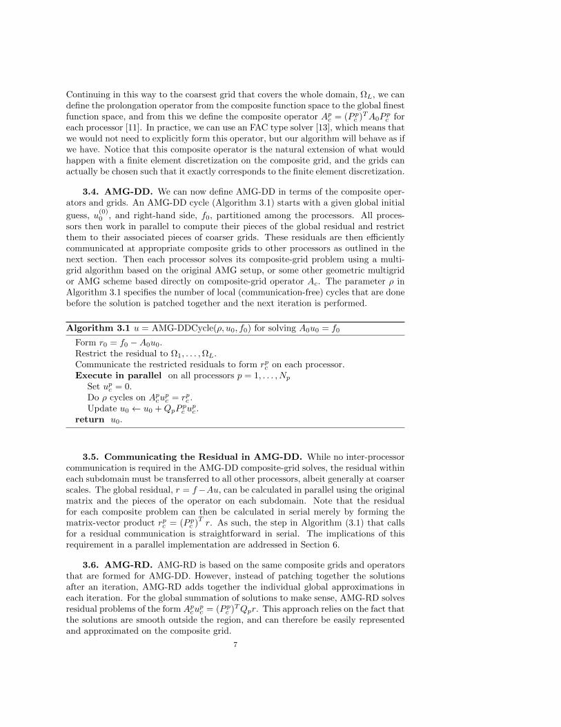
3.4. AMG-DD. We can now define AMG-DD in terms of the composite oper-ators and grids. An AMG-DD cycle (Algorithm 3.1) starts with a given global initial
guess, u(0)0 , and right-hand side, f0, partitioned among the processors. All proces-
sors then work in parallel to compute their pieces of the global residual and restrictthem to their associated pieces of coarser grids. These residuals are then efficientlycommunicated at appropriate composite grids to other processors as outlined in thenext section. Then each processor solves its composite-grid problem using a multi-grid algorithm based on the original AMG setup, or some other geometric multigridor AMG scheme based directly on composite-grid operator Ac. The parameter ρ inAlgorithm 3.1 specifies the number of local (communication-free) cycles that are donebefore the solution is patched together and the next iteration is performed.
Algorithm 3.1 u = AMG-DDCycle(ρ, u0, f0) for solving A0u0 = f0
Form r0 = f0 −A0u0.Restrict the residual to Ω1, . . . ,ΩL.Communicate the restricted residuals to form rpc on each processor.Execute in parallel on all processors p = 1, . . . , Np
Set upc = 0.Do ρ cycles on Apcu
pc = rpc .
Update u0 ← u0 +QpPpc u
pc .
return u0.
3.5. Communicating the Residual in AMG-DD. While no inter-processorcommunication is required in the AMG-DD composite-grid solves, the residual withineach subdomain must be transferred to all other processors, albeit generally at coarserscales. The global residual, r = f−Au, can be calculated in parallel using the originalmatrix and the pieces of the operator on each subdomain. Note that the residualfor each composite problem can then be calculated in serial merely by forming thematrix-vector product rpc = (P pc )
Tr. As such, the step in Algorithm (3.1) that calls
for a residual communication is straightforward in serial. The implications of thisrequirement in a parallel implementation are addressed in Section 6.
3.6. AMG-RD. AMG-RD is based on the same composite grids and operatorsthat are formed for AMG-DD. However, instead of patching together the solutionsafter an iteration, AMG-RD adds together the individual global approximations ineach iteration. For the global summation of solutions to make sense, AMG-RD solvesresidual problems of the form Apcu
pc = (P pc )TQpr. This approach relies on the fact that
the solutions are smooth outside the region, and can therefore be easily representedand approximated on the composite grid.
7

Algorithm 3.2 u = AMG-RDCycle(ρ, u0, f0) for solving A0u0 = f0
Require: ρ : Number of on-processor cycles.Require: u0 : Initial guess.Require: f0 : Right-hand side.
Form r0 = f0 −A0u0.Execute in parallel on all processors p = 1, . . . , Np
Set upc = 0.Do ρ cycles on APc u
pc = (P pc )TQpro.
Update u← u0 +∑p P
pc u
pc .
return u0.
4. Theory. This section establishes a two-level convergence theory for AMG-DD and AMG-RD. We first show that the two methods are duals of each other in theenergy inner product. We then develop an abstract theory that establishes optimalconvergence under full regularity and approximation property assumptions on theorigin of the global fine-grid matrix equation, Au = f . In particular, we assumethat A is symmetric and positive definite, and that this matrix equation was createdby conforming finite element discretization of a two- or three-dimensional uniformlyelliptic operator on a region that is either a convex polygon or has smooth boundary.Below, we assume further that the finite elements are chosen on the fine, composite,and coarse levels in such a way that they satisfy the strong approximation propertyand that ‖A‖ is bounded above in terms of the norm of the coarse-level matrix. Theseassumptions, while much more general, hold for continuous piecewise linear or bilinearelements on uniform grids that admit coarsening by a factor of 2.
In what follows, we use C to denote a generic constant, independent of the numberof processors and problem dimension, that may change meaning with each occurrence.Recall that Qp is the matrix that zeros out the entries in f outside processor p’ssubdomain, Dp
0 , but leaves f inside Dp0 unchanged. As before, we let Ωpc and Gpc
denote the respective composite grid and associated function space determined bythe global grids, Ωi, i = 0, 1, . . . , L. Also as before, we let P pc : Gpc → G0 denote theinterpolation operator from processor p’s composite grid to the fine grid, and writeApc = (P pc )TAP pc . Then, one iteration of AMG-DD starting with a zero initial guessis
u← ΣpQpPpc (Apc)
−1(P pc )T f.
The error propagation matrix for this method is
Md = I − ΣpQpPpc (Apc)
−1(P pc )TA. (4.1)
Similarly, one iteration of AMG-RD starting with a zero initial guess is
u← ΣpPpc (Apc)
−1(P pc )TQpf,
with the error propagation matrix
Mr = I − ΣpPpc (Apc)
−1(P pc )TQpA. (4.2)
Now, since the adjoint of any matrix B in the energy inner product < A·, · >is A−1BTA, then it is easy to see by the Euclidean symmetry of P pc (Apc)
−1(P pc )T
8

and Qp that Md and Mr are energy adjoints of each other. One take-home from thisresult is that the range and domain decomposition approaches exhibit the same energyconvergence bounds. Another is that we could use one of these methods following theother to create a symmetric iteration.
While it may be more natural to measure convergence of either error propagationmatrix in the energy norm, the Euclidean norm of Md may be simpler by virtue ofthe orthogonality of its individual terms. To see this for Md as defined in (4.1), letSp = P pc (Apc)
−1(P pc )TA, the energy-orthogonal projection of fine-grid vectors onto therange of P pc . Since the Qp sum to I, we have
‖Mdx‖2 =∑p
||Qp(I − Sp)x||2.
Our aim now is to show that ||Md|| is bounded uniformly above by a constant lessthan 1.
The bottom line here is that we need to know how well composite-grid vectorsapproximate fine-grid vectors in the corresponding subdomain. It can, of course,provide no approximation at all to oscillatory vectors outside Dp
0 – vectors that areenergy orthogonal to the composite grid. The key here is the presence of Qp, whichmeans that we just need to know the local accuracy in Dp
0 , where there is no de-refinement. To avoid estimates of the above sum from depending on the number ofprocessors, we need to localize the effect of x on these terms. Our convergence theorembelow shows that I − Sp has enough structure to allow us to write Qp(I − Sp)x interms of a component of x that is nonzero only on Dp
0 and some close neighborhoodabout it.
To achieve this structure, we content ourselves with a two-grid result, but withminimal padding in the sense that η0 = 1. We therefore now assume that eachcomposite grid, Ωpc , consists of Dp
0,1, the fine grid with uniform mesh spacing h onDp
0 and its nearest neighbors, and a 2h grid beyond that to the boundary, in whatwe call the de-refinement region, D = Ω1 − Dp
1 . Note that the composite grid hasonly coarse points in D. We begin with two assumptions that hold for our problemsetting. These assumptions are made with regard to a global coarsening of the finegrid by a factor of 2. In particular, let P (without a subscript) denote the operatorthat interpolates from the global coarse grid to the fine grid, and let P p1 denote theoperator that interpolates from the global coarse grid to p’s composite grid. Noticethat P p1 : G1 → Gpc , and A1 = (P p1 )TApcP
p1 .
Assume now that the following strong approximation property (SAP)[14, 15] holdsfrom the global coarse level to both the global fine and the composite levels, respec-
tively: Letting T = I−P(PTAP
)−1PTA and Tp = I−P p1
((P p1 )TApcP
p1
)−1(P p1 )TApc ,
then
||Tw|| ≤ C
||A||||Aw|| , ∀w ∈ G0, (4.3)
and
||Tpw|| ≤C
||Apc ||||Apcw|| , ∀w ∈ Gpc . (4.4)
Assume also that
‖A‖ ≤ C‖Apc‖. (4.5)
9
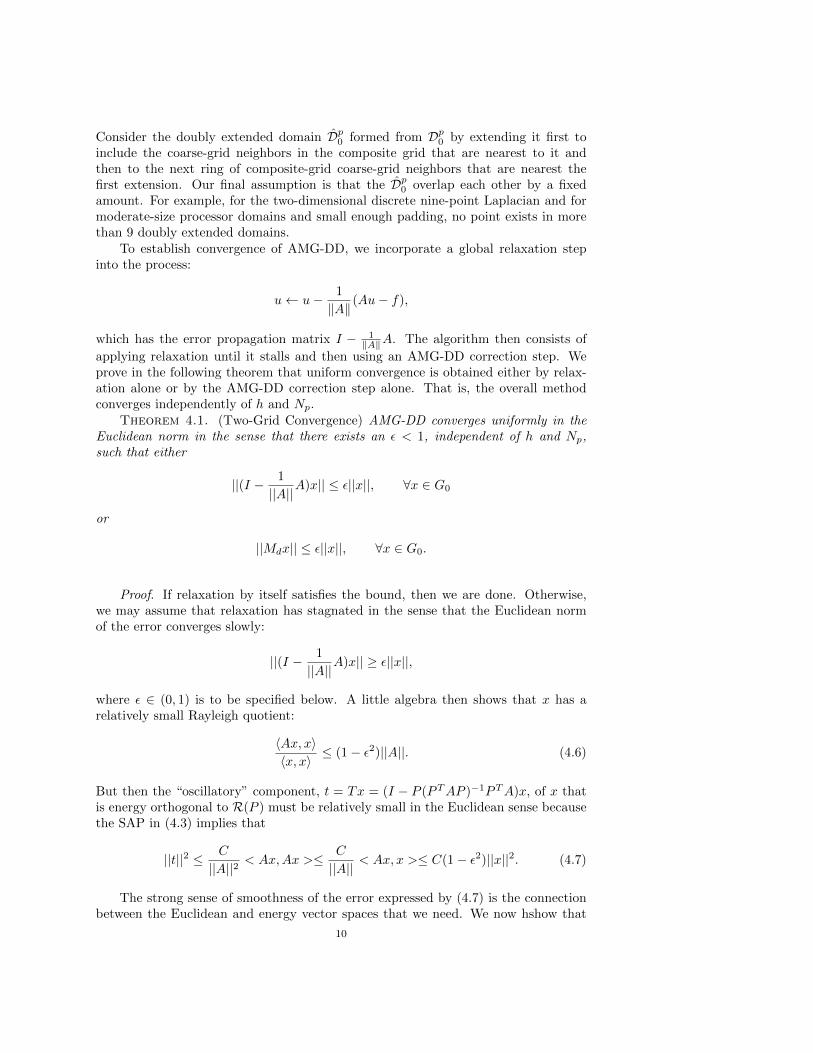
Consider the doubly extended domain Dp0 formed from Dp0 by extending it first toinclude the coarse-grid neighbors in the composite grid that are nearest to it andthen to the next ring of composite-grid coarse-grid neighbors that are nearest thefirst extension. Our final assumption is that the Dp0 overlap each other by a fixedamount. For example, for the two-dimensional discrete nine-point Laplacian and formoderate-size processor domains and small enough padding, no point exists in morethan 9 doubly extended domains.
To establish convergence of AMG-DD, we incorporate a global relaxation stepinto the process:
u← u− 1
‖A‖(Au− f),
which has the error propagation matrix I − 1‖A‖A. The algorithm then consists of
applying relaxation until it stalls and then using an AMG-DD correction step. Weprove in the following theorem that uniform convergence is obtained either by relax-ation alone or by the AMG-DD correction step alone. That is, the overall methodconverges independently of h and Np.
Theorem 4.1. (Two-Grid Convergence) AMG-DD converges uniformly in theEuclidean norm in the sense that there exists an ε < 1, independent of h and Np,such that either
||(I − 1
||A||A)x|| ≤ ε||x||, ∀x ∈ G0
or
||Mdx|| ≤ ε||x||, ∀x ∈ G0.
Proof. If relaxation by itself satisfies the bound, then we are done. Otherwise,we may assume that relaxation has stagnated in the sense that the Euclidean normof the error converges slowly:
||(I − 1
||A||A)x|| ≥ ε||x||,
where ε ∈ (0, 1) is to be specified below. A little algebra then shows that x has arelatively small Rayleigh quotient:
〈Ax, x〉〈x, x〉
≤ (1− ε2)||A||. (4.6)
But then the “oscillatory” component, t = Tx = (I − P (PTAP )−1PTA)x, of x thatis energy orthogonal to R(P ) must be relatively small in the Euclidean sense becausethe SAP in (4.3) implies that
||t||2 ≤ C
||A||2< Ax,Ax >≤ C
||A||< Ax, x >≤ C(1− ε2)||x||2. (4.7)
The strong sense of smoothness of the error expressed by (4.7) is the connectionbetween the Euclidean and energy vector spaces that we need. We now hshow that
10

the composite-grid step effectively reduces such error. Specifically, our aim now is toprove that there exists a constant c <∞ such that∑
p
||Qp(I − Sp)t||2 ≤ c||t||2, ∀t ∈ R⊥A(P ). (4.8)
We could then combine (4.7) and (4.8) to establish the convergence bound
‖Mdx‖2 =∑p
||Qp(I − Sp)x||2 =∑p
||Qp(I − Sp)t||2 ≤ cC(1− ε2)||x||2.
The last equality here follows because x differs from t by s ∈ R(P ) ⊂ R(P pc ), whichis in the null space of I − Sp. We could then complete the proof by choosing
ε =
√cC
1 + cC,
which, after a little algebra, reduces to the desired convergence bound.We are now left with the sole task of establishing (4.8). To this end, note that a
little more algebra yields∑p
||Qp(I − Sp)t||2 ≤ 2||t||2 + 2∑p
||QpSpt||2 .
Focusing on the last term of this inequality, for a given p, define rpc = (P pc )TAt. Itsuffices now to establish that∣∣∣∣QpP pc (Apc)
−1rpc∣∣∣∣ ≤ C
||Apc ||||rpc ||. (4.9)
Since ||QpP pc || = 1, this would follow if we could prove that
||τp|| ≤C
||Apc ||||Apcτp|| , (4.10)
where τp = (Apc)−1rpc . Since Tpτp = τp and P = P pc P
p1 , then more algebra yet shows
that τp ∈ R(P p1 )⊥Apc , with superscript ⊥Ap
cdenoting Apc -orthogonal complement. But
(4.10) follows directly from the SAP, (4.4), so we have thus established (4.9).P and P pc agree outside Dp0 , so PTAt = 0 implies that rpc is nonzero only on Dp0
and its nearest coarse-grid neighbors. Thus, ||(P pc )TAt|| only involves values of t onDp0 . Let tploc denote t restricted to Dp0 . We then use (4.9) to conclude that∣∣∣∣QpP pc (Apc)
−1(P pc )TAt∣∣∣∣ ≤ C
||Apc ||||A||||tploc||.
Finally, by the boundedness assumption, (4.5), on ||A||||Ap
c || and the limited overlap as-
sumption on Dp0 , we obtain∑p
||QpP pc (Apc)−1(P pc )TAt||2 ≤
∑p
C
minp ||Apc ||2||A||2||tploc||
2 ≤ C||t||2.
We have therefore established (4.8) and, thus, the proof.Remark 4.1. Theorem 1 establishes uniform convergence of AMG-DD in the
Euclidean norm. A direct consequence of this result is uniform convergence of itsdual, AMG-RD, in the residual norm:
||Mr||A2 ≡ ||AMrA−1|| = ||MT
d || ≤ ε < 1.
11

5. AMG-DD/RD Numerics. While the previous section establishes theoret-ical convergence properties of the method in a two-level setting, more nuanced ques-tions need to be addressed in practice. With the AMG-DD/RD algorithms, a verylarge parameter space must be explored if optimal choices are to be identified. Theparameters selected can have effects on the maximum possible size of the problemdue to the overlapping grids and on the time to solution as a function of computa-tion/communications required. To obtain some insight into good practical ranges forthese parameters, numerical tests were performed based on a simple model problemwhose convergence properties are well understood in the context of AMG methods.The results of these experiments are reported here. These results were then used todetermine reasonable choices for the parameters used to form the composite grids forthe model problem. We establish choices for the padding on each level that seemreasonable in terms of their effect on convergence and complexity or, in other words,on time to solution. We then attempt to determine how much computational workshould be expended on solving the composite grid subproblems before communicationis allowed between processors.
The numerical results described below were obtained from a sequential implemen-tation of the parallel AMG and AMG-DD algorithms. For AMG, we use V (1, 1) cycles(see Algorithm 2.1), hybrid Gauss-Seidel, and coarsening (i.e., inter-level transfer andcoarse-level operators) based on the classical Ruge-Stuben algorithm [5]. These par-ticular AMG parameter choices were made because they are fairly common, but otheralgorithmic choices would also lead to similar results and conclusions.
5.1. Size of Problem on a Processor. To model the computational cost ofthe AMG-DD algorithm, we have to first calculate the number of unknowns neededto form a composite problem. This is a function of the number of unknowns assignedto a processor, |Dp0 |, and the padding on each grid, ηi. It is important to note thatAMG-DD requires more memory than AMG to solve the same problem, so AMG cansolve somewhat larger problems on any given machine, depending on the size of thepadding.
As described earlier, the pad amount is the amount of nearest neighbors that weadd to a problem on each grid. To develop a closed form for this, we start out withthe assumption that the processor owns a region of the original problem of size nd
in d dimensions, and we assume a constant padding of η and a constant coarseningfactor c ≥ 2. We can show recursively that the length of the side of Dk,η, k = 0, . . . , L,satisfies
lk =n
ck+
k∑i=0
2η + αk−ici
≈ n
ck+
k∑i=0
2η
ci,
where each −1 < αk < 1 accounts for the fact that lk−1 may not be perfectly divisibleby c. The sizes of the Dk,η are then given by
|D0,η| = ld0 , |D1,η| = ld1 , . . . |DL−1,η| = ldL−1, |DL| = |ΩL|.
To get the total size of the composite grid, it is easier to first imagine that there areonly two grids, and then see that the size of the composite grid, |Ωc|, is the paddedfine region combined with the coarse grid outside of that region:
|Ωc| = |D0,η|+ |D1,η −D1| ≈ |D0,η|+ |D1,η| −|D0,η|cd
.
12

Fig. 5.1: Left: Growth of the composite grid for n = 100 as a function of η. Right:Effect of η on local problem size n under fixed memory constraints.
Now, using this same logic on all grids yields
|Ωc| = |D0,η|+ |D1,η −D1|+ · · ·+ |DL−1,η −DL−1|+ |ΩL −DL|
≈(
1− 1
cd
)ld0 +
(1− 1
cd
)ld1 + . . . .+
(1− 1
cd
)ldL−1 + |ΩL|
≈(
1− 1
cd
) L−1∑k=0
(n
ck+
k∑i=0
2η
ci
)d+ |ΩL|
≈(
1− 1
cd
) L−1∑k=0
(n
ck+ 2η
(c
c− 1
))d+ |ΩL|
= O(nd + nd−1η + · · ·+ nηd−1 + Lηd + |ΩL|
).
In particular, for the case of d = 2 dimensions and coarsening factor c = 2, we have
|Ωc| ≈ n2 + 12nη + 12Lη2 + |ΩL|.
Notice that the size of the composite grid depends on: n2, the size of the fine-gridregion assigned to a processor; Np, the number of processors on the machine (assuminga fully coarsened hierarchy of grids so that L ≈ log(N) ≈ log(Np)); and η, the sizeof the padding region. Considering this expression for n = 100 and several differentfixed numbers of processors, Figure 5.1 shows how |Ωc| scales with η and also how theproblem size n is affected under fixed memory constraints.
Notice that Figure 5.1 shows that keeping η small, especially on the order ofone or two, means that the size of the composite grid is essentially the same asthe size of the problem that would be assigned to a processor in a typical parallelimplementation. Changing the scale of the processors has very little effect on thegrowth of the composite problem size, especially for small padding amounts.
5.2. Parameter Effects on Convergence. One issue that needs to be ad-dressed is the ability of composite grids to approximate the solution on the fine-gridprocessor subdomains. Since AMG-DD is intended as a replacement for a V-cycle, itsconvergence factors are compared to that of a V-cycle for solving global problems ofthe same size. These results are presented in the context of weak scaling, that is, the
13

0 5 10 15 20 25 30 350
0.01
0.02
0.03
0.04
0.05
0.06
0.07
0.08
0.09
0.1
Composite Grid padding (η)
Con
verg
ence
Maximum converence as a function of padding
AMG p=9AMG−DD p=9AMG p=16AMG−DD p=16AMG p=25AMG−DD p=25AMG p=49AMG−DD p=49
0 5 10 15 20 25 30 350
1
2
3
4
5
6x 10
4
Composite Grid padding (η)
Com
plex
ity
Complexity as function of padding
AMG p=9AMG−DD p=9AMG p=16AMG−DD p=16AMG p=25AMG−DD p=25AMG p=49AMG−DD p=49
Fig. 5.2: Convergence and complexity (number of nonzeros in the composite-gridmatrix) as functions of uniform padding for varying numbers of processors: 9=red,16 = blue, 25 = green, and 49=pink. The AMG plots in the complexity graph showthe number of unknowns in the global fine grid.
number of unknowns per processor is fixed and the number of processors is varied.(We ignore memory constraints in these results; see earlier discussion and Figure 5.1.)
Figure 5.2 compares optimal convergence of the AMG-DD cycle, with η constantfor each grid, to a standard AMG V-cycle. To achieve this optimal convergence, wesolve each processor’s problem as well as we can before doing any communication. Thiswould of course only make sense if computation were actually “free”. In Figure 5.2,we also show problem complexity (i.e., the number of nonzeros in the composite-gridmatrix) on each processor as the padding increases for the case of uniform padding,which we present in relation to the number of unknowns in the global fine grid.
Figure 5.2 indicates that the composite problems can give good approximationto the global solution and, as expected, increasing the overlap between the processorsenhances the convergence rate for the algorithm. However, convergence must beunderstood in the context of the attendant complexity. The complexity graph showsus that, for minimal padding, the size of the problem on each processor is almostindependent of the size of the global problem, which is directly proportional to thenumber of processors. One question this leads to is how important it is to maintaina high level of padding outside of the fine-grid region.
Figure 5.3 is the same test as Figure 5.2, but now only η0 is allowed to grow, whileηk is fixed at 2 for all k > 0. Figure 5.3 shows that increasing the padding only onthe fine grid greatly reduces its effectiveness; however growth of the problem in thissetting is now directly tied just to the size of the fine grid patch on each processor,and is nearly independent of the number of processors and the global problem size.
In Table 5.1, we present sample convergence factors for parameters that are com-mensurate with the scaling models that we created for AMG-DD/AMG-RD. Eachprocessor was assigned 5000 points in the original fine grid, and tests were run withvarious padding levels determined by η = 1, 2, 3, and 4 and various numbers of localsolves per cycle determined by ρ = 1, 2, 3, and 4.
One important take-away from these results is that they appear to be almostindependent of the number of processors that we selected. There is mild growth asthe number of processors increases, but it is similar to growth exhibited by AMG.Convergence actually improves in some cases, but these fluxuations are quite smalland probably due to minor variations in the convergence rate of the AMG methodused to approximate the composite solves. Table 5.1 also indicates that, while it is
14

0 5 10 15 20 25 30 350
0.01
0.02
0.03
0.04
0.05
0.06
0.07
0.08
0.09
0.1
Composite Grid padding (η)
Con
verg
ence
Maximum converence as a function of padding
AMG p=9AMG−DD p=9AMG p=16AMG−DD p=16AMG p=25AMG−DD p=25AMG p=49AMG−DD p=49
0 5 10 15 20 25 30 350
1
2
3
4
5
6x 10
4
Composite Grid padding (η)
Com
plex
ity
Complexity as function of padding
AMG p=9AMG−DD p=9AMG p=16AMG−DD p=16AMG p=25AMG−DD p=25AMG p=49AMG−DD p=49
Fig. 5.3: Convergence and complexity (number of nonzeros in the composite-gridmatrix) as functions of fine-grid padding (coarse-grid padding is fixed at 2) for varyingnumbers of processors: 9=red, 16 = blue, 25 = green, and 49=pink. The AMG plotsin the complexity graph show the number of unknowns in the global fine grid.
NumProcessors = 9 NumProcessors = 16
ρ = 1 ρ = 2 ρ = 3 ρ = 4
η = 1 0.119 0.053 0.043 0.054η = 2 0.105 0.037 0.031 0.031η = 3 0.121 0.036 0.027 0.026η = 4 0.098 0.037 0.023 0.028
ρ = 1 ρ = 2 ρ = 3 ρ = 4
η = 1 0.142 0.071 0.064 0.062η = 2 0.139 0.058 0.050 0.041η = 3 0.127 0.048 0.028 0.041η = 4 0.123 0.043 0.027 0.030
NumProcessors = 25 NumProcessors = 36
ρ = 1 ρ = 2 ρ = 3 ρ = 4
η = 1 0.147 0.073 0.061 0.062η = 2 0.119 0.053 0.038 0.039η = 3 0.122 0.049 0.035 0.035η = 4 0.111 0.037 0.027 0.027
ρ = 1 ρ = 2 ρ = 3 ρ = 4
η = 1 0.146 0.070 0.071 0.068η = 2 0.156 0.061 0.058 0.045η = 3 0.152 0.060 0.037 0.036η = 4 0.128 0.044 0.031 0.039
Table 5.1: Convergence of AMG-DD for 9, 16, 25, and 36 processors with 5000 pointsper processor for varying padding (η) and number of cycles (ρ).
beneficial to perform two cycles on each processor before the residual is calculated,the benefit of any additional cycles is very mild. The table also suggests that anypadding past η = 2 does not generate significant increase in convergence of the overalliteration. The results for AMG-RD are omitted since, as expected, they are nearlyidentical to those for AMG-DD.
Based on the results from the model problem, it is clear to see that two linesof grid-point padding on each level yields an effective process. Using such a smallpadding means that the problem stays within an acceptable region in terms of theamount of memory that must be wasted in order to support the composite grids. Itis also clear that, within this framework for the model problem, only two iterationsshould be performed before communication is required. In all of the tests reportedhere, the local solves converged with a consistent factor of about 0.1, so ρ reallyreflects the number of decimal places of accuracy in the solution of the composite-gridequations. This suggests that, for the model problem, two decimal places of accuracy
15

is an appropriate target for the local composite-grid solves.
6. Parallel Issues. As we said above, to simplify the task of studying AMG-RDand AMG-DD in a large parameter space, we restrict ourselves to weak scaling testsin anticipation of relatively weak processor architectures. One goal of this study is toenvision modifications to AMG methods that may have better scaling characteristicsfor future generations of computers. As the number of processors increases, the cost ofcommunication, especially on coarser levels, affects the weak-scaling characteristics ofthese algorithms. Our investigation of these methods is in the context of the effects ofexascale computing on AMG algorithms, so strong-scaling is not studied here becausethe sheer size of the resulting problems would preclude such models.
We should also note that, in practice, not all communications are equal, andmachines are tending to become hierarchical in nature. As the number of processorsdramatically expand, we must reach a point where the subdomain contains a tinyfraction of the global problem, leaving the composite grid with extremely coarse gridson the global domain. We can thus expect convergence of AMG-RD and AMG-DDto stall at these extreme scales, unless we employ these methods in a hierarchicalway on subsets of processors (e. g., “nodes”) where communication may be relativelyinexpensive.
In a naive implementation, if the padding is allowed to grow, then communicationcosts would have significant drawbacks in parallel. However, in the previous section,the parameters that we identified fall into a regime where we can accumulate theresidual in a manner with little overhead. In fact, we introduce an algorithm here thatallows communication within a log(Np) communication pattern, but with a reducedconstant compared to a typical V-cycle.
6.1. Setup. Implementation of AMG-DD and AMG-RD can be done using onlythe constructs (coarse grids, coarse-grid operators, and intergrid transfer operators) ofan existing AMG hierarchy. As in all AMG algorithms, the cost of this setup processfor AMG-DD and AMG-RD becomes an issue. In a purely serial setting, setup costsfor AMG-DD and AMG-RD can be up to about twice that of standard AMG dueto the redundant calculation that we use. However, in parallel, the increase in setupcosts over that of AMG itself can be reduced essentially to the cost of communicatingthe necessary components of the operators to each processor. This is a result of thefact that the construction of the setup is based on existing AMG constructs. Thisadded cost is therefore bounded by that of performing one extra V-Cycle because thenecessary communication process can be done using the same pattern as used in theresidual communication process, described next.
6.2. Residual Communication in Parallel. Since each processor only needsthe residual on its composite grid, communication can be minimized by starting theresidual updates on the coarsest grid, ΩL, and bubbling the information up as detailedin Algorithm 6.1. The algorithm proceeds up through the hierarchy, exchanging datawith neighbors on each grid. For example, consider the one-dimensional illustrationin Figure 6.1. Every point in processor p’s composite grid can be labeled as being inat least one of three sets: Dp0 ∩ Ωk; a set Ψ of distance-ηk neighbors (indicated bysquares in the figure); or the composite grid Ψc formed from Ψ ∩ Ωk+1, which is acoarsening of some set Ψ. The algorithm sends Ψ and Ψc (which may be empty) toneighboring processors. As presented, it communicates redundant information, butthis is easy to modify in practice to reduce costs. We now show that the algorithmproduces the desired residual update, and we show later in Section 7.2.1 that the total
16

Algorithm 6.1 Collect residual for composite grids
for k = L→ 0 doExecute in parallel on all processors (p = 1, 2, . . . , Np)if (Dp0 ∩ Ωk) 6= ∅ then
Identify the set of neighboring processors p1, . . . , pm (not equal to p) thatcontain points within distance ηk of (Dp0 ∩ Ωk).for j = 1→ m do
Find all points x ∈ (Dp0 ∩ Ωk) such that dist(x, (Dpj0 ∩ Ωk)) ≤ ηk, let Ψ bethe union of these points.FormΨc from Ψ ∩ Ωk+1 as outlined in Section 3.2.Send the residual at all points and grids in Ψ,Ψc to pj .
end forend if
end for
Fig. 6.1: One-dimensional example of a processor’s composite grid and the residualupdate Algorithm 6.1. Processor p owns the points in the red vertical rectangle. Pointsin the distance-ηk neighborhood of p are highlighted with squares and numbered 0through 7. All other points are in the coarse composite grid of some distance-ηkneighbor and are labeled accordingly. Example sets Ψ and Ψc are also given.
amount of data communicated by each processor is on the same order as the numberof points on its boundary plus a log factor.
Claim: On grid Ωk, processor p owns region Dp0 ∩ Ωk . After the algorithm hasexecuted for this grid, processor p will have the correct residual for all points, denotedΩpc,k, on a composite grid built from Dp0 ∩ Ωk.
Proof. The needed information is assumed to be stored off processor; otherwise,the claim is trivially true.
• Suppose k = L (the coarsest grid). Then, since p communicates directly toall processors within ηL, it trivially has the correct residual for all x ∈ Ωpc,L.
• Suppose k = m, and assume that each processor has obtained residual infor-mation at all points on Ωpc,m+1, the composite grid formed from Dp0 ∩ Ωm+1.By construction, if x ∈ Ωpc,m, then there exists y ∈ Dp0 ∩ Ωm and a path ofthe form
y → ym,η ↓ y(m+1) → y(m+1),η ↓ y(m+2) → · · · → x.
17

Notice, for some processor q, that y(m+1) ∈ Dq0 ∩ Ωm+1 and x ∈ Ωqc,m+1.Hence, processor q has residual information for point x by assumption and,since y(m+1) is within distance ηm, then processor q passes that informationto processor p.
The claim thus holds.
This claim shows that, after the kth grid has been updated, each processor hasthe composite grid defined by the region it owns for that grid. Therefore, after allgrids have been updated, each processor obtains the residual information it needs forits composite grid. The cost of this algorithm is detailed in Section 7.2.
7. Parallel Numerics. Ideally, to judge the scaling characteristics of this algo-rithm, we would present results based on tests run on different architectures. How-ever, no fully parallel implementation of this algorithm has yet been developed, so weinstead rely on models that give us indications of how we expect AMG and AMG-DD/AMG-RD to scale. Much of the analysis of the scalability of a parallel implemen-tation of AMG is based on the work by Gahvari et al. [16]. Throughout this section,three main parameters are utilized:
1. α: The cost of latency on the machine per message. For now, we assume thatthis is a constant that does not depend on the distance of connections.
2. β: Inverse bandwidth cost or, more generically, the cost per amount of datasent.
3. γ: The flop rate of the machine, that is, the amount of work per computation.
Based on data in Table 2 from [16], we make the assumption that α, β, γ have thefollowing relations for the models:
α = 104γ β = 10γ .
We also assume, as before, that we are solving a nine-point discretization of a Lapla-cian in two dimensions, which allows us to predict stencil patterns in a full coarseningscenario. Also note that the models just describe the cost of V-cycles; setup modelingis omitted at this time.
7.1. AMG V-Cycle Cost. One standard process for modeling a parallel al-gorithm is to analyze the cost on the most expensive processor, so we follow thisstructure. In its most basic form, the model of one AMG V-Cycle can be written as
Tamg = Tlatency + Tcomm + Tcomp.
The communication terms can be modeled as
Tlatency + Tcomm =
L∑i=0
(αmi + βqi) ,
where L+ 1 is the number of grids in the system (note that L ≈ log(N), with N thenumber of unknowns in the system), mi is the number of messages sent on level i,and qi is the amount of data sent on level i. To calculate these numbers, we modelthe V (1, 1)-Cycle (Algorithm 2.1). To actually specify the parameters mi, qi, we needto understand the structure of the operators in the multigrid hierarchy. For thisanalysis, we assume standard geometric full coarsening by a factor of 2, so complexityand operators are identical on all grids.
18

7.1.1. Communication costs per AMG V-Cycle. For calculating the pa-rameters, let Γi denote the number of unknowns on the boundary of the processorof interest on grid i. Since we are modeling the amount of information required toadvance computation, then, to be precise, if the number of points on a side for a pro-cessor is r, the amount of information that needs to be gathered is 4r + 4. However,the effect of the four corner points is negligible, so we assume that, given ni pointson a side on grid i, we have
Γi = 4ni.
This also leads to the convenient relation Γi = Γ0
2i . Parameters mi, qi can now be splitinto their components for relaxation, residual calculation, restriction, interpolation,and coarse-grid solve.
First, we assemble the latencies:
mi =
2mi,relax +mi,residual +mi,restrict +mi,interp i < L
2mL,solve i = L.
For the case we are investigating, we have mi = 2 · 8 + 8 + 8 + 8 if i < L and 2 · 8 ifi = L. The latency cost can then be represented as
Tlatency = α
(L−1∑i=0
40 + 2 · 8
)= α(40L+ 16).
The amount of data sent is
qi =
2qi,relax + qi,residual + qi,restrict + qi,interp i < L
2 · qL,solve i = L,
which, for this case, is
qi =
2Γi + Γi + Γi
2 + Γi
2 i < L
2ΓL i = L.
The inverse bandwidth cost can be modeled as
Tcomm = β
(L−1∑i=0
4Γi + 2ΓL
)= β
(L−1∑i=0
4Γ0
2i+ 2
Γ0
2L
)' 8βΓ0.
7.1.2. Computation Costs per AMG V-Cycle. Assuming that there areW0 = n2 points on the finest grid, then the number of points, Wi, on the i-th grid is
Wi =W0
22i.
Computation cost is then based on the amount of work done on each grid. So, foreach grid, we can model the work in terms of the number of unknowns on individualgrids:
• Relaxation (Gauss-Seidel) : 18 operations• Restriction (Ideal) : 18
4 operations
19

0 1 2 3 4 5 6 70
1
2
3
4
5
6
7
8
9
log10
(NP)
log 10
(T)
W0 = 25,000
Tamg
Tlatency
Tcomm
Tcomp
0 1 2 3 4 5 6 70
1
2
3
4
5
6
7
8
9
log10
(NP)
log 10
(T)
W0 = 100,000
Tamg
Tlatency
Tcomm
Tcomp
Fig. 7.1: AMG V-Cycle costs for W0 = 25, 000 and 100, 000, respectively.
• Interpolation (Ideal) :184 operations
• Residual calculation: 18 operations• Coarse-grid solve : 2 relaxations = 36 operations.
This translates to per-grid costs of
N irelax = 18Wi, N i
restrict = 184 Wi, N i
interp = 184 Wi,
N iresidual = 18Wi, N i
solve = 36WL.
So the total computational cost is
Tcomp = γ
(L−1∑i=0
2N irelax +
L−1∑i=0
N iresidual +
L−1∑i=0
N irestrict +
L−1∑i=0
N iinterp +Nsolve
)
= γW0
[63
(1− (1/4)L
1− (1/4)
)+
36
22L
]' 84γW0.
7.1.3. Graphs for AMG Costs. For the purpose of modeling, we scale bysetting γ = 1. For a problem with Np processors and n2 unknowns per processor,then L = dlog4(Np · n2)e, W0 = n2, and Γ0 = 4n. Using the derived functions for theAMG costs, the models for a V (1, 1)-Cycle for Np = 2i, i = 1, . . . , 20, while holdingthe number of unknowns per processor constant yields Figure 7.1. Notice that thisfigure shows that the only term that grows significantly as the number of processorsincreases is latency.
7.2. AMG-DD Cycle Cost. As in the derivation of costs for AMG, we againbreak the problem down into three parts:
Tamgdd = Tlatency + Tcomm + Tcomp.
First, we have to be specific about the form of the algorithm that we are modeling.The assumption here is that there already has been an AMG setup, and the partsof the matrix needed to solve the composite problems have already been distributed.Therefore, we restrict ourselves to modeling the solve cycles of AMG-DD from Algo-rithm 3.1.
20

7.2.1. Communication Costs per AMG-DD Cycle. There are three mainpoints of communication with the AMG-DD cycle: residual calculation; residual re-striction; and communication of the composite residuals. Residual calculation andrestriction, respectively, cost
mresidual = 8, qresidual = Γ0
mrestriction = 8L, qrestriction = Γ0
2
(1−(1/2)L
1−1/2
).
For the communication of the residual, we model the algorithm developed for AMG-DD (Algorithm 6.1). To simplify the model so that the number of neighboring proces-sors is fixed on all grid levels, we assume that η is appropriately reduced to a smallervalue on coarse grids. This is likely the best way to design the algorithm for parallelcomputation anyway. We do not, however, account for this reduction in the commu-nication term, hence the model considered here is slightly more pessimistic than itshould be for this latency-friendly case. Since nearest-neighbor communication is allthat is required on each grid, then the latency cost is just
mres.comm =
L∑i=0
8 = 8(L+ 1).
To bound the amount of data sent in Algorithm 6.1, we can use the result derivedin Section 5.1 for the size of the composite grid. Given a fixed side length, n, on aprocessor and a fixed padding, η, on each grid, then the amount of data communicatedis proportional to
|Ωc| − n2 ≈ n2 + 12nη + 12Lη2 + |ΩL| − n2.
Hence, if |ΩL| is small, we can take
qres.comm = 12nη + 12Lη2.
Notice that the total amount of data that must be communicated in the residualcommunication routine is on the order of the size of the boundary on a processor plusa log factor.
The communication costs are then
Tlatency = α(8 + 8L+ 8(L+ 1)) = 16α(L+ 1)
and
Tcomm = β
(Γ0 +
Γ0
2
(1− (1/2)L
1− 1/2
)+ 12nη + 12Lη2
)' β
(2Γ0 + 12nη + 12Lη2
).
7.2.2. Computation Costs per AMG-DD Cycle. Using the work from theAMG derivations and the assumption thatW0 is the size of the fine grid on a processor,we know that the residual computation costs
Nresidual.comp = 19W0.
21

0 1 2 3 4 5 6 70
1
2
3
4
5
6
7
8
9
log10
(NP)
log 10
(T)
W0 = 25,000
TAMG−DD
Tlatency
Tcomm
Tcomp
0 1 2 3 4 5 6 70
1
2
3
4
5
6
7
8
9
log10
(NP)
log 10
(T)
W0 = 100,000
TAMG−DD
Tlatency
Tcomm
Tcomp
Fig. 7.2: AMG-DD costs for W0 = 25, 000 and 100, 000, with η = 2 and ρ = 1.
Restriction requires 18 operations, and must be done for each grid, so
Nrestrict.comp =
L∑i=1
18W0
22i= 18W0
(1− (1/4)L
1− (1/4)
)' 36W0.
Finally, solving the composite problems can be estimated in the same fashion as foran AMG V-cycle, except that we now replace W0 with the calculated size of thecomposite grid, |Ωc|, and then add the parameter ρ that represents the number ofcycles done between calculations:
Namgdd.comp = ρ|Ωc|[63
(1− (1/4)L
1− (1/4)
)+
36
22L
],
where ρ is on the order of two to three. This yields a total computation cost of
Tcomp = γ
(19W0 + 18W0
(1− (1/4)L
1− (1/4)
)+ ρ|Ωc|
[63
(1− (1/4)L
1− (1/4)
)+
36
22L
])' γ (43W0 + ρ84|Ωc|) .
7.2.3. Graphs for AMG-DD. Using these derivations, we present scalingmodels in Figures 7.2 and 7.3 for AMG-DD cycles for a select sample of parame-ters. First, we fix the padding at η = 2 and the number of points per processor atW0 = 25, 000 and 100, 000, and then present the models for ρ = 1. Second, we modelthe scaling characteristics for larger padding, η = 20, fixing ρ = 2, for processor sizesW0 = 25, 000 and 100, 000. The effect of doing more, or less, computation (chang-ing ρ) merely shifts the scale of computation up. For any ρ > 2, cost savings fromreducing communication are lost by the increased time in computation.
Figures 7.2 and 7.3 show that, as desired, the AMG-DD algorithm achieves thegoal of reducing communication for computation. While latency and communicationboth increase as the number of processors increases, the computation cost is now whatdrives the overall time per iteration of the algorithm. The amount of computationthat has been added to each processor, as shown in Section 7.2.2, is on the same orderof magnitude as the standard approach, so these figures also serve to highlight thebalance between computation and communication that already exists in traditionalAMG implementations.
22

0 1 2 3 4 5 6 70
1
2
3
4
5
6
7
8
9
log10
(NP)
log 10
(T)
W0 = 25,000
TAMG−DD
Tlatency
Tcomm
Tcomp
0 1 2 3 4 5 6 70
1
2
3
4
5
6
7
8
9
log10
(NP)
log 10
(T)
W0 = 100,000
TAMG−DD
Tlatency
Tcomm
Tcomp
Fig. 7.3: AMG-DD costs for W0 = 25, 000 and 100, 000, with η = 20 and ρ = 2
.
8. Conclusion. Two new algebraic solvers, AMG-RD and AMG-DD, were devel-oped and analyzed here that aim to trade communication for computation by formingglobal composite “grids” based only on the matrix, not the geometry. This trade-off isachieved efficiently by way of global composite grids on each processor that enable fullsubdomain overlap, but primarily at very coarse scales of resolution. One advantageof this approach is that it allows for the construction of composite problems with noprior knowledge of the original grid structure, but forms them algebraically, basedonly on components of an existing AMG setup. An important development of thismethodology is a novel residual communication process that enables effective parallelcomputation on composite grids, avoiding the all-to-all communication costs of thegeometric methods. The main purpose of this paper was to study the potential ofthese two algebraic methods as possible alternatives to existing AMG approaches forfuture parallel machines. To this end, we developed some theoretical properties ofthese methods and reported on serial numerical tests of their convergence propertiesover a spectrum of problem parameters. We also included a parameter study basedon a performance model designed to anticipate their potential for use in emergingparallel architectures.
Our cost models show that these methods compete as algebraic solvers with cur-rent AMG algorithms on modern large-scale computers, but may surpass them in a sig-nificant way only if and when future architectures come with increased communication-to-computation cost ratios. This is, however, less of a limitation of the AMG-DD andAMG-RD algorithms than a testament to the scaling efficiency of current parallelAMG methods, and future research on improvements in the use of composite gridsmay tip the balance in favor of these new approaches.
An important aspect of AMG-DD and AMG-RD that we have not yet exploredis the potential for use in a nested iteration (or full multigrid) process: While thesemethods seem comparable to AMG solvers in terms of algebraic convergence factors,they may prove to be very effective when used to reduce the error to discretization-error levels. Specifically, if we apply a nested iteration approach to the composite gridsubproblems (which requires no communication between processors), it may well bethat the resulting error will be acceptable in the sense that it is comparable to the errorin the discrete solution itself–relative to the solution of the underlying PDE (assuming
23

here that there is one). These methods may thus be able to deliver acceptable resultswith only one communication phase. This capability could substantially reduce thecommunication costs that currently inhibit the use of full multigrid algorithms inlarge-scale parallel applications. Future work will therefore focus on the study ofthese methods in a nested iteration context.
REFERENCES
[1] Brandt A, Diskin B. Multigrid solvers on decomposed domains. Domain Decomposition Methodsin Science and Engineering: The Sixth International Conference on Domain Decomposi-tion, Contemporary Mathematics, vol. 157, American Mathematical Society: Providence,Rhode Island, 1994; 135–155.
[2] Mitchell W. A parallel multigrid method using the full domain partition. Electron. Trans.Numer. Anal. 1998; 6:224–233.
[3] Bank RE, Holst MJ. A new paradigm for parallel adaptive meshing algorithms. SIAM J. Sci.Stat. Comp. 2000; 22:1411–1443.
[4] Brandt A, McCormick S, Ruge J. Algebraic multigrid (AMG) for sparse matrix equations. InSparsity and its Applications, D.J, Evans (ed.)., 1984; 257–284.
[5] Ruge J, Stuben K. Algebraic multigrid (AMG). In Multigrid Methods, vol. 5, McCormick SF(ed.). SIAM: Philadelphia, PA., 1986.
[6] Mitchell W. Parallel adaptive multilevel methods with full domain partitions. App. Num. Anal.and Comp. Math. 2004; 1:36–48.
[7] Bank RE, Lu S. A domain decomposition solver for a parallel adaptive meshing paradigm.SIAM J. Sci. Comput. 2004; 26(1):105–127.
[8] Bank RE, Vassilevski PS. Convergence analysis of a domain decomposition paradigm. Comput.Visual Sci. 2008; 11:333–350.
[9] Bank RE. Some variants of the Bank and Holst parallel adaptive meshing paradigm. Comput.Vis. Sci. Oct 2006; 9(3):133–144.
[10] Bank RE, Jimack P. A new parallel domain decomposition method for the adaptive finiteelement solution of elliptic partial differential equations. Concurrency Computat.: Pract.Exper. 2001; 13:327–350.
[11] Bank RE, Lu S, Tong C, Vassilevski PS. Scalable parallel algebraic multigrid solvers. TechnicalReport UCRL-TR-210788, Lawrence Livermore National Laboratory, Livermore, Califor-nia 2004.
[12] Henson VE, Yang UM. Boomeramg : A parallel algebraic multigrid solver and preconditioner.Applied Numerical Mathematics April2002; 41:155177.
[13] McCormick S. Multilevel Adaptive Methods for Partial Differential Equations. No. 6 in Frontiersin Applied Mathematics, SIAM, 1989.
[14] Hackbusch W. Survey of convergence proofs for multi-grid iterations. Special topics of appliedmathematics : functional analysis, numerical analysis, and optimization : proceedings ofthe seminar held at the GMD, Bonn, 8-10 October 1979, Frehse J, Pallaschke D, Trotten-berg U (eds.). North-Holland Pub.: Amsterdam, 1980; 151–164.
[15] Vassilevski PS. Coarse spaces by algebraic multigrid: multigrid convergence and upscaling errorestimates. Advances in Adaptive Data Analysis 2011; 3(01n02):229–249.
[16] Gahvari H, Gropp W, Jordan KE, Schulz M, Yang UM. Modeling the performance of an al-gebraic multigrid cycle using hybrid mpi/openmp. 2012 41st International Conference onParallel Processing 2012; 0:128–137.
24