Embed Size (px)
Citation preview

HAL Id: tel-00659362https://tel.archives-ouvertes.fr/tel-00659362
Submitted on 12 Jan 2012
HAL is a multi-disciplinary open accessarchive for the deposit and dissemination of sci-entific research documents, whether they are pub-lished or not. The documents may come fromteaching and research institutions in France orabroad, or from public or private research centers.
L’archive ouverte pluridisciplinaire HAL, estdestinée au dépôt et à la diffusion de documentsscientifiques de niveau recherche, publiés ou non,émanant des établissements d’enseignement et derecherche français ou étrangers, des laboratoirespublics ou privés.
Multidisciplinary Design Optimization of LaunchVehicles
Mathieu Balesdent
To cite this version:Mathieu Balesdent. Multidisciplinary Design Optimization of Launch Vehicles. Optimization andControl [math.OC]. Ecole Centrale de Nantes (ECN), 2011. English. �tel-00659362�

ÉCOLE DOCTORALESCIENCES POUR L’INGÉNIEUR, GÉOSCIENCES,
ARCHITECTURE
École Centrale de NantesAnnée 2011
Thèse de DoctoratSpécialité : Génie Mécanique
présentée et soutenue publiquement par
Mathieu BALESDENTle 3 novembre 2011
à l’Office National d’Etudes et de Recherches Aérospatiales
OPTIMISATION MULTIDISCIPLINAIRE DELANCEURS
(Multidisciplinary Design Optimization of Launch Vehicles)
JURY
Président :Jean-Antoine Désidéri Directeur de Recherche, INRIA
Rapporteurs :David Bassir Docteur, HDR, Université de Technologie de Belfort-Montbéliard
Attaché pour la Science et la Technologie, Ministère des Affaires EtrangèresPatrick Siarry Professeur, Université Paris-Est Créteil Val-de-Marne
Examinateurs :Philippe Dépincé Professeur, Ecole Centrale de NantesMichèle Lavagna Associate Professor, Politecnico di MilanoRodolphe Le Riche Docteur, HDR, CNRS - Ecole des Mines de Saint-Etienne
Invités :Nicolas Bérend Ingénieur, OneraJulien Laurent-Varin Docteur, CNES
Directeur de thèse : Philippe DÉPINCÉEncadrant Onera : Nicolas BÉRENDLaboratoires : Office National d’Etudes et de Recherches Aérospatiales
Institut de Recherche en Communications et Cybernétique de NantesN◦ E.D. : 498-196


ACKNOWLEDGMENTS
This work has been realized in the Onera’s System Design and Performance EvaluationDepartment, in collaboration with the CNES Launchers Directorate and the team SystemsEngineering Products, Performance and Perceptions of IRCCyN. I would like to thank thedirector of DCPS, Dr. Donath, for giving me the opportunity to achieve this thesis at Onera.
I would like to thank Dr. Désidéri, who did me the honour of chairing my PhD commit-tee. I express my gratitude to Dr. Bassir and Prof. Siarry for reviewing this PhD thesis. Ialso thank Dr. Laurent-Varin, Prof. Lavagna and Dr. Le Riche for accepting to be part ofmy PhD committee.
I would like to acknowledge Prof. Dépincé for agreeing to be my advisor during thesethree years. I would like to express my thankfulness to my Onera supervisor, M. Bérend forhis comments, suggestions, edits, and advices during the thesis.
I would like to thank my CNES supervisor, M. Oswald. I thank also M. Amouroux forhis help in the elaboration of the launch vehicle disciplinary models.
I owe a great amount of thanks to the people whom I’ve been working with every day atthe Onera’s DCPS. Especially, I thank Dr. Piet-Lahanier for her numerous advices all alongthe thesis.
I would also like to thank the Onera PhD students (Dalal, Ariane, Rata, Walid, Julien,Joseph, François, Yohan and Damien) who have provided the most exciting working envi-ronment. Special thanks go to my office mate, Rudy, qui quæsivit rerum causas, for thosenumerous happy hours spent during the thesis.
Last but not least, I would like to thank my parents, who believed in me and alwaysencouraged me. Finally, I would especially like to thank my fiancée Sophie, for all her loveand for her understanding when I spent my time working on this thesis. I appreciate hersupport and her sacrifices very much during this endeavor.
This PhD thesis has been co-funded by CNES and Onera.


Non est ad astra mollis e terris via.There is no easy way from the earth to the stars.
Hercules FurensSeneca the Younger


To Sophie, Cécile & Claude


Contents
Nomenclature 13
Acronyms 15
Introduction 17
I Panorama of Multidisciplinary Design Optimization methodsused in Launch Vehicle Design 21
1 Generalities about Multidisciplinary Design Optimization 231.1 Introduction . . . . . . . . . . . . . . . . . . . . . . . . . . . . . . . . . . . . 231.2 Mathematical formulation of the general MDO problem . . . . . . . . . . . . 24
1.2.1 Problem formulation . . . . . . . . . . . . . . . . . . . . . . . . . . . 251.2.2 Types of variables . . . . . . . . . . . . . . . . . . . . . . . . . . . . . 251.2.3 Types of constraints . . . . . . . . . . . . . . . . . . . . . . . . . . . 261.2.4 Types of functions . . . . . . . . . . . . . . . . . . . . . . . . . . . . 261.2.5 Disciplinary equations . . . . . . . . . . . . . . . . . . . . . . . . . . 261.2.6 Coupling . . . . . . . . . . . . . . . . . . . . . . . . . . . . . . . . . . 271.2.7 Multidisciplinary analysis . . . . . . . . . . . . . . . . . . . . . . . . 28
1.3 Feasibility concepts in MDO . . . . . . . . . . . . . . . . . . . . . . . . . . . 281.3.1 Individual disciplinary feasibility . . . . . . . . . . . . . . . . . . . . 281.3.2 Multidisciplinary feasibility . . . . . . . . . . . . . . . . . . . . . . . 29
1.4 Description of the Launch Vehicle Design problem . . . . . . . . . . . . . . . 291.4.1 Disciplines and variables . . . . . . . . . . . . . . . . . . . . . . . . . 291.4.2 Constraints . . . . . . . . . . . . . . . . . . . . . . . . . . . . . . . . 301.4.3 Objective functions . . . . . . . . . . . . . . . . . . . . . . . . . . . . 301.4.4 Specificities of the Launch Vehicle Design problem . . . . . . . . . . . 30
1.5 Conclusion . . . . . . . . . . . . . . . . . . . . . . . . . . . . . . . . . . . . . 31
2 Classical MDO methods 332.1 Introduction . . . . . . . . . . . . . . . . . . . . . . . . . . . . . . . . . . . . 332.2 Single level methods . . . . . . . . . . . . . . . . . . . . . . . . . . . . . . . 34
2.2.1 Multi Discipline Feasible . . . . . . . . . . . . . . . . . . . . . . . . . 34
1

2.2.2 Individual Discipline Feasible . . . . . . . . . . . . . . . . . . . . . . 362.2.3 All At Once . . . . . . . . . . . . . . . . . . . . . . . . . . . . . . . . 38
2.3 Qualitative comparison of the single level methods . . . . . . . . . . . . . . . 392.4 Multi level methods . . . . . . . . . . . . . . . . . . . . . . . . . . . . . . . . 40
2.4.1 Collaborative Optimization . . . . . . . . . . . . . . . . . . . . . . . 402.4.2 Modified Collaboration Optimization . . . . . . . . . . . . . . . . . . 422.4.3 Concurrent SubSpace Optimization . . . . . . . . . . . . . . . . . . . 442.4.4 Bi-Level Integrated Systems Synthesis . . . . . . . . . . . . . . . . . 462.4.5 Analytical Target Cascading . . . . . . . . . . . . . . . . . . . . . . . 492.4.6 Other multi level methods . . . . . . . . . . . . . . . . . . . . . . . . 51
2.5 Conclusion . . . . . . . . . . . . . . . . . . . . . . . . . . . . . . . . . . . . . 52
3 Optimization algorithms and optimal control techniques 533.1 Introduction . . . . . . . . . . . . . . . . . . . . . . . . . . . . . . . . . . . . 533.2 Optimization algorithms used in MDO . . . . . . . . . . . . . . . . . . . . . 54
3.2.1 Gradient-based algorithms . . . . . . . . . . . . . . . . . . . . . . . . 543.2.2 Gradient-free algorithms . . . . . . . . . . . . . . . . . . . . . . . . . 55
3.3 Optimal control . . . . . . . . . . . . . . . . . . . . . . . . . . . . . . . . . . 623.3.1 Direct methods . . . . . . . . . . . . . . . . . . . . . . . . . . . . . . 643.3.2 Indirect methods . . . . . . . . . . . . . . . . . . . . . . . . . . . . . 653.3.3 Single vs multiple shooting methods . . . . . . . . . . . . . . . . . . . 663.3.4 Collocation methods . . . . . . . . . . . . . . . . . . . . . . . . . . . 683.3.5 Dynamic Programming . . . . . . . . . . . . . . . . . . . . . . . . . . 69
3.4 Conclusion . . . . . . . . . . . . . . . . . . . . . . . . . . . . . . . . . . . . . 69
4 Analysis of the MDO method application in the Launch Vehicle Design 714.1 Introduction . . . . . . . . . . . . . . . . . . . . . . . . . . . . . . . . . . . . 714.2 Different study cases and optimization criteria . . . . . . . . . . . . . . . . . 72
4.2.1 MDO methods and optimization algorithms . . . . . . . . . . . . . . 724.2.2 Optimization criteria and different study cases . . . . . . . . . . . . . 73
4.3 Trajectory handling . . . . . . . . . . . . . . . . . . . . . . . . . . . . . . . . 734.4 Comparison of the main MDO methods in a common application case . . . . 74
4.4.1 Presentation of the optimization problem . . . . . . . . . . . . . . . . 744.4.2 Comparison of AAO, MDF and CO . . . . . . . . . . . . . . . . . . . 744.4.3 Comparison of FPI, AAO, BLISS2000 and MCO . . . . . . . . . . . . 75
4.5 Comparative synthesis of the main MDO methods . . . . . . . . . . . . . . . 764.5.1 Calculation costs and convergence speed . . . . . . . . . . . . . . . . 764.5.2 Considerations about optimality conditions . . . . . . . . . . . . . . . 764.5.3 Method deftness . . . . . . . . . . . . . . . . . . . . . . . . . . . . . 77
4.6 Conclusion and ways of improvement . . . . . . . . . . . . . . . . . . . . . . 784.6.1 Inclusion of design stability aspects in the optimization process . . . 784.6.2 Trajectory optimization in the design process . . . . . . . . . . . . . 794.6.3 Heuristics and gradient-based algorithms coupling . . . . . . . . . . . 794.6.4 Another subdivision of the optimization process . . . . . . . . . . . . 79

II Multidisciplinary Design Optimization formulations using astage-wise decomposition 81
5 Presentation of the stage-wise decomposition formulations 835.1 Introduction . . . . . . . . . . . . . . . . . . . . . . . . . . . . . . . . . . . . 835.2 Decomposition of the problem and identification of the couplings . . . . . . . 85
5.2.1 Definition of the launch vehicle design problem . . . . . . . . . . . . 855.2.2 Decomposition of the state vector dynamics . . . . . . . . . . . . . . 875.2.3 Determination of the coupling variables . . . . . . . . . . . . . . . . . 885.2.4 Proposition of the optimization strategy . . . . . . . . . . . . . . . . 89
5.3 Stage-wise decomposition formulations . . . . . . . . . . . . . . . . . . . . . 915.3.1 First formulation . . . . . . . . . . . . . . . . . . . . . . . . . . . . . 915.3.2 Second formulation . . . . . . . . . . . . . . . . . . . . . . . . . . . . 935.3.3 Third formulation . . . . . . . . . . . . . . . . . . . . . . . . . . . . . 955.3.4 Fourth formulation . . . . . . . . . . . . . . . . . . . . . . . . . . . . 96
5.4 Conclusion . . . . . . . . . . . . . . . . . . . . . . . . . . . . . . . . . . . . . 98
6 Application case : optimization of a three-stage-to-orbit launch vehicle 996.1 Introduction . . . . . . . . . . . . . . . . . . . . . . . . . . . . . . . . . . . . 996.2 Description of the disciplines . . . . . . . . . . . . . . . . . . . . . . . . . . . 100
6.2.1 Propulsion . . . . . . . . . . . . . . . . . . . . . . . . . . . . . . . . . 1006.2.2 Aerodynamics . . . . . . . . . . . . . . . . . . . . . . . . . . . . . . . 1026.2.3 Trajectory . . . . . . . . . . . . . . . . . . . . . . . . . . . . . . . . . 1026.2.4 Mass budget and geometry design . . . . . . . . . . . . . . . . . . . . 106
6.3 Optimization variables and disciplinary interactions . . . . . . . . . . . . . . 1096.3.1 Optimization variables . . . . . . . . . . . . . . . . . . . . . . . . . . 1096.3.2 Interactions between the different disciplines . . . . . . . . . . . . . . 109
6.4 MDO problem formulation . . . . . . . . . . . . . . . . . . . . . . . . . . . . 1106.4.1 Initial formulation . . . . . . . . . . . . . . . . . . . . . . . . . . . . 1106.4.2 MDF formulation . . . . . . . . . . . . . . . . . . . . . . . . . . . . . 110
6.5 Stage-wise decomposition formulations . . . . . . . . . . . . . . . . . . . . . 1116.5.1 First formulation . . . . . . . . . . . . . . . . . . . . . . . . . . . . . 1116.5.2 Second formulation . . . . . . . . . . . . . . . . . . . . . . . . . . . . 1136.5.3 Third formulation . . . . . . . . . . . . . . . . . . . . . . . . . . . . . 1146.5.4 Fourth formulation . . . . . . . . . . . . . . . . . . . . . . . . . . . . 115
6.6 Conclusion . . . . . . . . . . . . . . . . . . . . . . . . . . . . . . . . . . . . . 116
7 Comparison of the different formulations 1177.1 Introduction . . . . . . . . . . . . . . . . . . . . . . . . . . . . . . . . . . . . 1177.2 Analysis of the problem dimensionality and the number of constraints . . . . 1187.3 Qualitative comparison of proposed formulations . . . . . . . . . . . . . . . . 1207.4 Numerical comparison of the formulations . . . . . . . . . . . . . . . . . . . 122
7.4.1 Context . . . . . . . . . . . . . . . . . . . . . . . . . . . . . . . . . . 1227.4.2 Adaptation of stage-wise formulations to genetic algorithm . . . . . . 1247.4.3 Results and analysis . . . . . . . . . . . . . . . . . . . . . . . . . . . 125

7.4.4 Limitations of the numerical comparison . . . . . . . . . . . . . . . . 1327.5 Conclusion . . . . . . . . . . . . . . . . . . . . . . . . . . . . . . . . . . . . . 132
III Optimization strategies dedicated to the stage-wise decom-position 135
8 Optimization strategies 1378.1 Introduction : needs and context . . . . . . . . . . . . . . . . . . . . . . . . 1378.2 Description of the proposed optimization strategy . . . . . . . . . . . . . . . 1388.3 Phase I : Exploratory phase - initialization process . . . . . . . . . . . . . . . 140
8.3.1 Exploratory phase : search of a feasible initialization at the system level1408.3.2 Initialization process at the subsystem level . . . . . . . . . . . . . . 141
8.4 Phase II : first optimization phase . . . . . . . . . . . . . . . . . . . . . . . . 1428.4.1 Phase II (a) : first optimization phase using the Nelder & Mead algorithm1428.4.2 Phase II (b) : first optimization phase using the Efficient Global Op-
timization algorithm . . . . . . . . . . . . . . . . . . . . . . . . . . . 1438.5 Phase III : second optimization phase . . . . . . . . . . . . . . . . . . . . . . 144
8.5.1 Description of the optimization phase . . . . . . . . . . . . . . . . . . 1448.5.2 Expression of the system level sensitivities . . . . . . . . . . . . . . . 145
8.6 Convergence considerations . . . . . . . . . . . . . . . . . . . . . . . . . . . 1498.7 Conclusion . . . . . . . . . . . . . . . . . . . . . . . . . . . . . . . . . . . . . 151
9 Analysis of the optimization strategy 1539.1 Introduction . . . . . . . . . . . . . . . . . . . . . . . . . . . . . . . . . . . . 1539.2 Determination of the reference design . . . . . . . . . . . . . . . . . . . . . . 1549.3 Analysis of phase I : initialization strategy . . . . . . . . . . . . . . . . . . . 1579.4 Analysis of phase II : first optimization phase . . . . . . . . . . . . . . . . . 158
9.4.1 Comparison of Nelder & Mead and Genetic Algorithm . . . . . . . . 1589.4.2 Analysis of the Efficient Global Optimization algorithm . . . . . . . . 159
9.5 Analysis of phase III : second optimization phase . . . . . . . . . . . . . . . 1619.5.1 Accuracy of the gradient estimation . . . . . . . . . . . . . . . . . . . 1619.5.2 Performance of the proposed gradient-based approach . . . . . . . . . 161
9.6 Analysis of the whole optimization process . . . . . . . . . . . . . . . . . . . 1639.7 Optimization process efficiency . . . . . . . . . . . . . . . . . . . . . . . . . 1669.8 Conclusion . . . . . . . . . . . . . . . . . . . . . . . . . . . . . . . . . . . . . 167
Conclusion 169
A Dry mass sizing module 173A.1 Tanks . . . . . . . . . . . . . . . . . . . . . . . . . . . . . . . . . . . . . . . 173A.2 Turbopumps . . . . . . . . . . . . . . . . . . . . . . . . . . . . . . . . . . . . 175A.3 Pressurant system . . . . . . . . . . . . . . . . . . . . . . . . . . . . . . . . . 176A.4 Combustion chamber . . . . . . . . . . . . . . . . . . . . . . . . . . . . . . . 177A.5 Nozzle . . . . . . . . . . . . . . . . . . . . . . . . . . . . . . . . . . . . . . . 178

A.6 Engine . . . . . . . . . . . . . . . . . . . . . . . . . . . . . . . . . . . . . . . 179A.7 Offset mass for models adjustment . . . . . . . . . . . . . . . . . . . . . . . 180
B MDF robustness study and considerations about the Fixed Point Iteration181B.1 Robustness of the MDF method . . . . . . . . . . . . . . . . . . . . . . . . . 181B.2 Considerations about the use of the Fixed Point Iteration . . . . . . . . . . . 182
C Global Sensitivity Equation and Post-Optimality Analysis 183C.1 Global Sensitivity Equation . . . . . . . . . . . . . . . . . . . . . . . . . . . 183C.2 Post-Optimality Analysis . . . . . . . . . . . . . . . . . . . . . . . . . . . . . 184
D Demonstration of optimality conditions 187D.1 KKT conditions for the AAO formulation . . . . . . . . . . . . . . . . . . . 187D.2 KKT conditions for the first formulation . . . . . . . . . . . . . . . . . . . . 189D.3 Equivalence between the first and the third formulations . . . . . . . . . . . 193
E Résumé étendu de la thèse 197Introduction . . . . . . . . . . . . . . . . . . . . . . . . . . . . . . . . . . . . . . . 197E.1 Panorama des méthodes MDO utilisées dans la conception de lanceurs . . . 199
E.1.1 Formulation d’un problème MDO et concepts généraux . . . . . . . . 200E.1.2 Description du problème de conception de lanceurs . . . . . . . . . . 201E.1.3 Méthodes MDO classiques . . . . . . . . . . . . . . . . . . . . . . . . 202E.1.4 Synthèse comparative de l’application des méthodes MDO dans la con-
ception de lanceurs . . . . . . . . . . . . . . . . . . . . . . . . . . . . 204E.2 Formulations MDO utilisant une décomposition en étages . . . . . . . . . . . 206
E.2.1 Introduction . . . . . . . . . . . . . . . . . . . . . . . . . . . . . . . . 206E.2.2 Présentation des formulations SWORD . . . . . . . . . . . . . . . . . 207E.2.3 Présentation du cas d’application . . . . . . . . . . . . . . . . . . . . 208E.2.4 Comparaison des différentes formulations à MDF . . . . . . . . . . . 212E.2.5 Conclusion . . . . . . . . . . . . . . . . . . . . . . . . . . . . . . . . . 214
E.3 Stratégie d’optimisation dédiée à la décomposition en étages . . . . . . . . . 214E.3.1 Identification des besoins . . . . . . . . . . . . . . . . . . . . . . . . . 214E.3.2 Description de la stratégie d’optimisation . . . . . . . . . . . . . . . . 215E.3.3 Analyse des performances de la stratégie d’optimisation . . . . . . . . 218
Conclusion . . . . . . . . . . . . . . . . . . . . . . . . . . . . . . . . . . . . . . . . 219
F Publications and communications 223
References 225
Index 241
5


List of Figures
1 Classical Launch Vehicle Design decomposition . . . . . . . . . . . . . . . . . 19
1.1 Used nomenclature . . . . . . . . . . . . . . . . . . . . . . . . . . . . . . . . 251.2 Disciplinary analyzer and disciplinary evaluator . . . . . . . . . . . . . . . . 28
2.1 MDF method . . . . . . . . . . . . . . . . . . . . . . . . . . . . . . . . . . . 352.2 IDF method . . . . . . . . . . . . . . . . . . . . . . . . . . . . . . . . . . . . 372.3 AAO method . . . . . . . . . . . . . . . . . . . . . . . . . . . . . . . . . . . 392.4 CO method . . . . . . . . . . . . . . . . . . . . . . . . . . . . . . . . . . . . 422.5 MCO method . . . . . . . . . . . . . . . . . . . . . . . . . . . . . . . . . . . 442.6 CSSO method . . . . . . . . . . . . . . . . . . . . . . . . . . . . . . . . . . . 462.7 BLISS method . . . . . . . . . . . . . . . . . . . . . . . . . . . . . . . . . . . 482.8 BLISS2000 method . . . . . . . . . . . . . . . . . . . . . . . . . . . . . . . . 492.9 ATC method . . . . . . . . . . . . . . . . . . . . . . . . . . . . . . . . . . . 50
3.1 Nelder and Mead algorithm . . . . . . . . . . . . . . . . . . . . . . . . . . . 573.2 Basic scheme of an evolutionary algorithm . . . . . . . . . . . . . . . . . . . 583.3 Different ways to perform the crossover . . . . . . . . . . . . . . . . . . . . . 593.4 Example of mutation . . . . . . . . . . . . . . . . . . . . . . . . . . . . . . . 593.5 Example of kriging model . . . . . . . . . . . . . . . . . . . . . . . . . . . . 613.6 Single shooting vs multiple shooting methods for a four-section trajectory . . 683.7 Interpolation using Lagrange polynomials . . . . . . . . . . . . . . . . . . . . 69
5.1 Decomposition of the state vector dynamics . . . . . . . . . . . . . . . . . . 885.2 SWORD formulations . . . . . . . . . . . . . . . . . . . . . . . . . . . . . . 98
6.1 Propulsive parameters models . . . . . . . . . . . . . . . . . . . . . . . . . . 1016.2 Drag coefficient as a function of the Mach number . . . . . . . . . . . . . . . 1026.3 Earth-centered, Earth-fixed reference frame . . . . . . . . . . . . . . . . . . . 1046.4 Example of control law . . . . . . . . . . . . . . . . . . . . . . . . . . . . . . 1066.5 Dry mass sizing module . . . . . . . . . . . . . . . . . . . . . . . . . . . . . 1076.6 Evolution of the load factor coupling coefficient with respect to the maximal
axial load factor . . . . . . . . . . . . . . . . . . . . . . . . . . . . . . . . . . 1086.7 Results obtained with dry mass model . . . . . . . . . . . . . . . . . . . . . 1086.8 N2 Chart for one stage . . . . . . . . . . . . . . . . . . . . . . . . . . . . . . 110
7
LIST OF FIGURES
7.1 Search domain and number of constraints at the system level w.r.t. the num-ber of stages . . . . . . . . . . . . . . . . . . . . . . . . . . . . . . . . . . . . 119
7.2 Statistical results of the comparison . . . . . . . . . . . . . . . . . . . . . . . 1267.3 Results obtained for the 8th random initialization . . . . . . . . . . . . . . . 1277.4 Average improvement of the objective function during the optimization . . . 1307.5 Representation of the qualitative comparison with a radar chart . . . . . . . 1317.6 Average best found design and elapsed time to find a first feasible design . . 132
8.1 Optimization strategy . . . . . . . . . . . . . . . . . . . . . . . . . . . . . . 1398.2 Exploration strategy . . . . . . . . . . . . . . . . . . . . . . . . . . . . . . . 1418.3 Initialization at the subsystem level . . . . . . . . . . . . . . . . . . . . . . . 1428.4 Handling of design and coupling variables . . . . . . . . . . . . . . . . . . . . 145
9.1 Representation of the optimal trajectory . . . . . . . . . . . . . . . . . . . . 1549.2 Optimal trajectory and geometry . . . . . . . . . . . . . . . . . . . . . . . . 1569.3 Evolution of the objective function around the reference optimum . . . . . . 1569.4 Search domain of the position and velocity coupling variables . . . . . . . . . 1579.5 Comparison of Genetic and Nelder & Mead algorithms . . . . . . . . . . . . 1589.6 Results obtained with EGO . . . . . . . . . . . . . . . . . . . . . . . . . . . 1609.7 Real map (2500 points) and kriged maps (50 points) around the optimum . . 1619.8 Synthesis of the results obtained for the different phases . . . . . . . . . . . 1659.9 Example of phase III algorithm’s behavior . . . . . . . . . . . . . . . . . . . 1659.10 Evolution of the objective function during the optimization process . . . . . 1669.11 Evolution of the objective function during the optimization using EGO and
gradient-based algorithm . . . . . . . . . . . . . . . . . . . . . . . . . . . . . 166
A.1 Tank sizing module . . . . . . . . . . . . . . . . . . . . . . . . . . . . . . . . 173A.2 Turbopumps sizing module . . . . . . . . . . . . . . . . . . . . . . . . . . . . 175A.3 Pressurant system sizing module . . . . . . . . . . . . . . . . . . . . . . . . . 176A.4 Combustion chamber sizing module . . . . . . . . . . . . . . . . . . . . . . . 177A.5 Propulsive parameters . . . . . . . . . . . . . . . . . . . . . . . . . . . . . . 178A.6 Nozzle sizing module . . . . . . . . . . . . . . . . . . . . . . . . . . . . . . . 179
C.1 Coupled system . . . . . . . . . . . . . . . . . . . . . . . . . . . . . . . . . . 183
E.1 Principe général de SWORD . . . . . . . . . . . . . . . . . . . . . . . . . . . 207E.2 Formulations SWORD : hiérarchique (gauche) et non hiérarchique (droite) . 208E.3 Diagramme N2 . . . . . . . . . . . . . . . . . . . . . . . . . . . . . . . . . . 209E.4 Dimension de l’espace de recherche et nombre de contraintes . . . . . . . . . 212E.5 Comparaison des méthodes dans le cas d’une recherche globale . . . . . . . . 213E.6 Synthèse des résultats obtenus . . . . . . . . . . . . . . . . . . . . . . . . . . 213E.7 Stratégie d’optimisation . . . . . . . . . . . . . . . . . . . . . . . . . . . . . 215E.8 Stratégie d’exploration . . . . . . . . . . . . . . . . . . . . . . . . . . . . . . 216E.9 Processus d’optimisation en phase 3 . . . . . . . . . . . . . . . . . . . . . . . 217E.10 Comportement du processus d’optimisation . . . . . . . . . . . . . . . . . . . 218E.11 Comparaison des dispersions des points avant et après optimisations . . . . . 219
8

LIST OF FIGURES
E.12 Evolution de la fonction objectif pendant le processus d’optimisation . . . . 219
9


List of Tables
1.1 Different feasibility concepts and corresponding involved variables . . . . . . 29
2.1 Qualitative synthesis of the single level methods . . . . . . . . . . . . . . . . 40
4.1 Different MDO methods applied to launch vehicle design . . . . . . . . . . . 724.2 Different study cases of the MDO methods . . . . . . . . . . . . . . . . . . . 73
5.1 Characteristics of the proposed formulations . . . . . . . . . . . . . . . . . . 98
7.1 Synthesis of the optimization problems complexity at the system level . . . . 1197.2 Search space dimension and number of constraints at the system and subsys-
tem levels . . . . . . . . . . . . . . . . . . . . . . . . . . . . . . . . . . . . . 1207.3 Qualitative comparison of the different formulations . . . . . . . . . . . . . . 1207.4 Bounds of the optimization variables . . . . . . . . . . . . . . . . . . . . . . 1237.5 Used GA parameters for the comparison . . . . . . . . . . . . . . . . . . . . 1257.6 Average number of generations required to find a feasible design . . . . . . . 1297.7 Qualitative synthesis of the comparison . . . . . . . . . . . . . . . . . . . . . 131
9.1 Variables for the reference optimum design . . . . . . . . . . . . . . . . . . . 1559.2 Comparison between global random and proposed initialization process . . . 1579.3 EGO parameters . . . . . . . . . . . . . . . . . . . . . . . . . . . . . . . . . 1599.4 Accuracy of the gradient estimation . . . . . . . . . . . . . . . . . . . . . . . 1629.5 Results obtained for the validation of the second optimization phase . . . . . 1629.6 Results obtained for the phase I . . . . . . . . . . . . . . . . . . . . . . . . . 1639.7 Results obtained for the phase II . . . . . . . . . . . . . . . . . . . . . . . . 1649.8 Results obtained for phase III . . . . . . . . . . . . . . . . . . . . . . . . . . 1649.9 Summary of the results . . . . . . . . . . . . . . . . . . . . . . . . . . . . . . 1659.10 Dispersion of the found designs . . . . . . . . . . . . . . . . . . . . . . . . . 166
B.1 Results of the MDF robustness study . . . . . . . . . . . . . . . . . . . . . . 181B.2 Results of the Fixed Point Iteration study . . . . . . . . . . . . . . . . . . . 182
E.1 Différents concepts de faisabilité et variables associées . . . . . . . . . . . . . 201E.2 Comparaison qualitative des méthodes mono niveau . . . . . . . . . . . . . . 203
11


Nomenclature
MDO variables
z Design variablesy Coupling variablesx State variables
MDO functions and constraints
c Coupling functionsf Objective functiong Inequality constraintsh Equality constraintsR ResidualsX State variable computation functionsJ Subsystem-level intermediary objective functionss State dynamics functions
Launch vehicle design variables
D Stage diameterDne Nozzle exit diameterIsp Specific impulseMp Propellant massMd Dry massnf Axial load factorPc Chamber pressurePe Nozzle exit pressureq Mass flow rateRm Mixture ratioTW
Thrust to weight ratio
Trajectory variables
r Radiusv Velocityu Controlα Angle of attackγ Flight path angleθ Pitch angle
13

NOMENCLATURE
Notations
zsh Shared design variableszk Design variables specific to the kth subsystemz∗ Local copies of zz Approximation of zz◦ Feasible zzd Design variables present in the subsystem databasez Estimation of zzd Design variableszc Control variablesz′di Design variables of the ith stage intervening in other stage dynamicsXc State variable computation functions ensuring the consistency of the couplingsx Mean value of xσx Standard deviation of xf ∗ Optimized value of f
14

Acronyms
AAO All At OnceATC Analytical Target CascadingBLISS Bi-Level Integrated System SynthesisCO Collaborative OptimizationCSSO Concurrent SubSpace OptimizationDIV E Discipline Interaction Variable EliminationEGO Efficient Global OptimizationELV Expendable Launch VehicleFD Finite DifferencesFPI Fixed Point IterationGA Genetic AlgorithmGAGGS Genetic Algorithm Guided Gradient SearchGLOW Gross Lift-Off WeightGSE Global Sensitivity EquationGTO Geostationary Transfer OrbitIDF Individual Discipline FeasibleKKT Karush-Kuhn-TuckerLDC Local Distributed CriteriaLH2 Liquid HydrogenLOX Liquid OxygenLV D Launch Vehicle DesignMCO Modified Collaborative OptimizationMDA MultiDisciplinary AnalysisMDF MultiDiscipline FeasibleMDO Multidisciplinary Design OptimizationMDOIS Multidisciplinary Design Optimization based on Independent SubspacesMOPCSSO Multi-Objective Pareto Concurrent SubSpace OptimizationMSTO Multi Stage To OrbitNAND Nested ANalysis and DesignNLP Non Linear ProgrammingOBD Optimization Based DecompositionPOA Post-Optimality AnalysisPOST Program to Optimize Simulated TrajectoriesPSO Particle Swarm OptimizationRLV Reusable Launch Vehicle
15

ACRONYMS
RP Rocket PropellantRSM Response Surface MethodSA Simulated AnnealingSAND Simultaneous ANalysis and DesignSQP Sequential Quadratic ProgrammingSNN Single NAND NANDSSA System Sensitivity AnalysisSSN Single SAND NANDSSS Single SAND SANDSSTO Single Stage To OrbitSWORD Stage-Wise decomposition for Optimal Rocket Design
16

Introduction
Since the beginning of the XXth century and the works of Konstantin Tsiolkovsky concerningthe multi stage rocket design, published in 1903 in “The Exploration of Cosmic Space byMeans of Reaction Devices” , the design of launch vehicles has been constantly growing andhas become a strategic domain for it enables the access to space. Launch Vehicle Design(LVD) is a very complex optimization process in which the slightest mistake may induce eco-nomical, material and human disastrous consequences (e.g. explosion of the brazilian VLSlaunch vehicle in 2002). This sector, due to the development of many new launch vehiclesover the last few years, has been becoming more and more competitive. For this reason, it isprimordial to be able to design more and more efficient launch vehicles i.e. able to put intoorbit ever increasing payloads at the lesser cost, ensuring an acceptable level of reliability atthe same time. This requires in early design studies an efficient optimization process so asto explore a very large search space in order to quickly obtain an appropriate launch vehicleconfiguration which meets the given mission requirements.
LVD involves numerous disciplines such as aerodynamics, structure, trajectory, massbudget, etc. These disciplines require specific tools and may result in conflicting decisions.For instance, the choice of a large stage diameter has antagonistic effects on launcher per-formance through aerodynamics and structural sizing. This induces a very complex designprocess which includes the search of multidisciplinary compromises. Therefore, in additionto the mastery of disciplinary technologies, LVD requires system-oriented design methodolo-gies in order to organize the design process.
The classical engineering design method used in LVD consists of a loop between thedifferent disciplinary tasks. At each iteration of this loop, each discipline is reoptimizedaccording to the data given by the previous discipline. It gives to the next discipline newdata, in function of the results obtained during its own optimization. Thus, this designprocess needs several iterations to converge, may present some problems in order to find (ifnecessary) the compromises between the disciplines and may not lead to the global optimaldesign. Consequently, LVD requires the use of adapted tools in order to exploit the couplingsbetween the different disciplines, to make the compromise search easier, and to improve therobustness and the efficiency of the whole design process.
Multidisciplinary Design Optimization (MDO), is a research field of engineering scienceswhich aims at elaborating design methodologies devoted to solving complex multidisciplinarydesign problems. To this end, MDO regroups several topics such as the elaboration of newdesign problem formulations, the creation and the use of meta models in order to reducethe calculation time, the handling of uncertainties in order to improve the robustness or the
17

INTRODUCTION
elaboration of new optimization algorithms when the classical algorithms are inefficient.Many MDO methods can be found in literature [Balling and Sobieszczanski-Sobieski,
1994; Alexandrov and Hussaini, 1995; Sobieszczanski-Sobieski and Haftka, 1997; Agte et al.,2009; Tosserams et al., 2009]. These methods can be decomposed into two categories, withregard to the presence of one or several optimization levels.
The most used MDO method in LVD is the MultiDiscipline Feasible (MDF) method[Duranté et al., 2004; Tsuchiya and Mori, 2004; Bayley and Hartfield, 2007]. This singlelevel method splits up the design problem according to the different disciplines and asso-ciates a global optimizer (system level) and disciplinary analysis tools (subsystem level).In order to ensure the consistency of the couplings, this method involves at the subsystemlevel a multidisciplinary analysis (MDA). The MDF method makes the search of the globaloptimum easier with respect to the classical engineering method because it uses a singleoptimizer which handles all the design variables. Moreover, this method allows the searchof disciplinary compromises, thanks to the use of the MDA. Nevertheless, the handling ofall the design variables by the single optimizer may induce a very large search space. Thismay pose several problems such as the requirement of an appropriate initialization and agood knowledge of the design variable search domain in order to converge. Therefore, thismethod is only adapted to small design problems for which the search domain can be wellknown in advance.
In order to address more important design problems, some MDO methods involvingseveral levels of optimization have been proposed. These methods (e.g. Collaborative opti-mization and its derivatives [Braun and Kroo, 1995; Alexandrov and Lewis, 2000; DeMigueland Murray, 2000], Bi-Level Integrated Systems Synthesis [Sobieszczanski-Sobieski et al.,1998, 2000], etc.) decompose the design problem according to the different disciplines. Theyuse disciplinary optimizers at the subsystem level and a global optimizer at the system levelin order to coordinate the different disciplinary optimizations while optimizing the globalobjective function.
LVD is a specific MDO problem. Indeed, it involves a dynamical system to optimizeand combines the optimizations of the design variables and the trajectory. The trajectoryoptimization induces a trajectory simulation with stage separations. This latter involvesa highly non linear ordinary differential equation system which is complex to integrate.Moreover, the trajectory is coupled with all the other disciplines and is subjected to strictequality constraints, due to the mission requirements. These constraints are very difficult tosatisfy and considerably limit the feasible search domain i.e. the domain for which all theconstraints are satisfied.
All the MDO methods applied to LVD in literature use a decomposition of the designproblem into the different disciplines (Fig. 1). In such a decomposition, the trajectory ismost often considered as a black box for the optimizer and is optimized in the same wayas the other disciplines. Therefore, this decomposition may not be the most adapted tothe specific LVD problem. Another decomposition of the design problem which exploits thecouplings between the trajectory and the design variable optimization seems to be a valuableway of improvement of the whole optimization process.
18

OPTIMIZATION ALGORITHM
Objective : minimum Gross-Lift-Off-WeightConstraints : design constraints
specifications of mission coupling constraints
Propulsion
Structure
Cost estimation
Aerodynamics
Weights and Sizing
Trajectory
Recurrent cost
Development cost
Insurance cost
Other costs
Figure 1: Classical Launch Vehicle Design decomposition
This thesis is focused on the elaboration of new MDO methods dedicated to LVD. Thesemethods, called Stage-Wise decomposition for Optimal Rocket Design (SWORD), allow toplace the trajectory optimization at the center of the design process. The SWORD methodstransform the initial complex design optimization problem into the coordination of smallersingle stage MDO problems, which are easier to solve. To this end, new MDO formulationsof the LVD problem and an associated optimization strategy are proposed. The SWORDmethods are analyzed and compared to the most used MDO method in literature (MDF).
This manuscript is organized into three parts. The first part is devoted to drawing up apanorama of the MDO methods used in LVD. Chapter 1 presents the fundamental conceptsused to describe a general MDO process. In Chapter 2, we detail the main MDO methodsapplied in LVD. Chapter 3 concerns the description of the main optimization algorithmsused in MDO and the different techniques employed to perform the trajectory optimization.Finally, Chapter 4 details the analysis of the application of the MDO methods in LVD, andexpresses some possible ways of improvement with regard to this specific MDO problem.
The second part of this document is related to the description and the analysis of theproposed MDO formulations. To this end, we express in Chapter 5 four MDO formulationsin order to solve the LVD problem. Chapter 6 is devoted to the description of the applicationcase selected in this study : the optimization of three-stage-to-orbit launch vehicle for theminimization of the Gross-Lift-Off-Weight. Finally, Chapter 7 compares the SWORD for-mulations with the most used MDO method, theoretically and numerically in case of globalsearch study.
19

INTRODUCTION
The last part of this document is devoted to the description and the analysis of theproposed optimization strategy dedicated to the SWORD formulations. To this end, thispart is organized into two chapters. Chapter 8 concerns the elaboration of the optimizationstrategy. In this chapter, we detail the different parts of the optimization strategy and wedescribe the proposed optimization algorithms. Finally, Chapter 9 describes the numericalanalysis of the optimization strategy. In this chapter, we analyze each of the optimizationstrategy phases and we study the performance of the whole optimization process (i.e. MDOformulation and optimization algorithms), in terms of calculation time, quality of the op-timum and robustness to the initialization. Finally, we conclude on the efficiency of theSWORD methods, their use in Launch Vehicle Design preliminary studies and we detailseveral ways of improvement.
The appendices present some model considerations concerning the application case, anddetail some optimization techniques and mathematical demonstrations used in Chapter 8.The last appendix is constituted of an extended abstract of this thesis written in French.
20

Part I
Panorama of Multidisciplinary DesignOptimization methods used in Launch
Vehicle Design
21


Chapter 1
Generalities about MultidisciplinaryDesign Optimization
Contents1.1 Introduction . . . . . . . . . . . . . . . . . . . . . . . . . . . . . . 231.2 Mathematical formulation of the general MDO problem . . . . 24
1.2.1 Problem formulation . . . . . . . . . . . . . . . . . . . . . . . . . . 251.2.2 Types of variables . . . . . . . . . . . . . . . . . . . . . . . . . . . 251.2.3 Types of constraints . . . . . . . . . . . . . . . . . . . . . . . . . . 261.2.4 Types of functions . . . . . . . . . . . . . . . . . . . . . . . . . . . 261.2.5 Disciplinary equations . . . . . . . . . . . . . . . . . . . . . . . . . 261.2.6 Coupling . . . . . . . . . . . . . . . . . . . . . . . . . . . . . . . . 271.2.7 Multidisciplinary analysis . . . . . . . . . . . . . . . . . . . . . . . 28
1.3 Feasibility concepts in MDO . . . . . . . . . . . . . . . . . . . . . 281.3.1 Individual disciplinary feasibility . . . . . . . . . . . . . . . . . . . 281.3.2 Multidisciplinary feasibility . . . . . . . . . . . . . . . . . . . . . . 29
1.4 Description of the Launch Vehicle Design problem . . . . . . . 291.4.1 Disciplines and variables . . . . . . . . . . . . . . . . . . . . . . . . 291.4.2 Constraints . . . . . . . . . . . . . . . . . . . . . . . . . . . . . . . 301.4.3 Objective functions . . . . . . . . . . . . . . . . . . . . . . . . . . . 301.4.4 Specificities of the Launch Vehicle Design problem . . . . . . . . . 30
1.5 Conclusion . . . . . . . . . . . . . . . . . . . . . . . . . . . . . . . 31
1.1 IntroductionMultidisciplinary Design Optimization (MDO), also named Multidisciplinary Optimizationis a relatively recent field of engineering sciences whose objective is to address more effi-ciently design problems incorporating different disciplines. The MDO has been used in agreat number of domains such as structure, automotive, electronics or aerospace engineering,and allows to solve complex problems which are difficult to handle with the classical designmethods. This research field could grow up thanks to the increase of computation powerin the second half of the XXth century. Indeed, this increase has made the numerical opti-
23

CHAPTER 1. GENERALITIES ABOUT MULTIDISCIPLINARY DESIGNOPTIMIZATION
mization of complex problems possible and has paved the way for the complete system design.
By handling the different disciplines simultaneously, the MDO techniques facilitate thesearch of the global optimal design, which might not be obtained when the disciplines arehandled sequentially. Indeed, in most of the design problems, the different disciplines maylead to antagonistic decisions (e.g. structure and aerodynamics in launch vehicle design, aswe shall see later). In such cases, the MDO techniques aim to find compromises between thedifferent disciplines in order to reach the global optimal design.
Handling at the same time a series of disciplines increases significantly the complexity ofthe problem to solve. One of the branches of the MDO field is dedicated to the elaborationof new formulations of the optimization problem which aim at reducing the complexity ofthe problem and at allowing the more efficient use of the traditional optimization methods.The works presented in this document lie within this scope.
Instead of disciplinary codes in a computer or computer networks, the MDO may alsoaddress design problems involving engineer teams all over the world. Indeed, due to the glob-alization of the industries, the system design can be split up into different research centerslocated in different countries. In this case, the data exchanges between the teams become acrucial point of the design process and MDO provides new tools for the designers in orderto make the design process more efficient.
This part is devoted to the description of the application of the MDO methods to theLaunch Vehicle Design. The first chapter of this part concerns the presentation of the fun-damental concepts necessary to describe a MDO process. In the second chapter, we presentthe main MDO methods used in literature. The third chapter concerns the description ofthe classical optimization algorithms used in a MDO process and the main optimal controlmethodologies. Finally, in the fourth chapter, we analyze the application of the MDO meth-ods in Launch Vehicle Design in order to compare the different presented methods and topropose several ways of improvement.
1.2 Mathematical formulation of the general MDOproblem
In this section, we define the fundamental notions necessary to describe a classical MDOprocess. The Launch Vehicle Design problem can be decomposed into different ways. Thesedecompositions imply different optimization architectures. Indeed, the different disciplinescan be considered separately or can be optimized simultaneously inside a same system.Hereinafter, we will use, with the same signification, both terms discipline and subsystem,in order to describe the different processes at the subsystem level (Fig. 1.1). A subsystemmay regroup several disciplines and can be a part of a system to optimize (e.g. a stage of alaunch vehicle). In this section, we firstly describe the general mathematical formulation of aMDO problem and then we expose the different involved variables, functions and constraints.Finally, we detail the different ways to handle the disciplinary equations and couplings.
24

1.2. MATHEMATICAL FORMULATION OF THE GENERAL MDO PROBLEM
1.2.1 Problem formulationThe general formulation of a MDO problem can be written as follows :Formulation I.1 (General MDO formulation)
Minimize f(x, y, z)With respect to z ∈ Z
Subject to g(x, y, z) ≤ 0 (1.1)h(x, y, z) = 0 (1.2)
∀i ∈ {1, · · · , n},∀j 6= i, yi = {cji(xj, yj, zj)}j (1.3)∀i ∈ {1, · · · , n}, Ri(xi, yi, zi) = 0 (1.4)
A general MDO process is illustrated in Figure 1.1. All the different variables and functionsintervening in the MDO process will be described in the following sections.
Subsystem 1
z
min f(x,y,z)
g(x,y,z)<0
h(x,y,z)=0
i, R (x ,y ,z )=0
i, j=i, y ={c (x ,y ,z )}
MULTIDISCIPLINARY DESIGN OPTIMIZATION PROCESS
R (x ,y ,z)=0 or x =X (z,y )11 1
Multidisciplinary analysis
i i i i
ji j j ji
c1
cn
c i
1 1 1
Subsystem i
R (x ,y ,z)=0 or x =X (z,y )ii i i i i
Subsystem n
R (x ,y ,z)=0 or x =X (z,y )nn n n nn
Figure 1.1: Used nomenclature
1.2.2 Types of variablesA general MDO process involves several types of variables. These variables play specificroles and are used at the different steps of the MDO process. We can differentiate threecategories of variables in a general MDO problem:
• z : design variables. These variables evolve all along the optimization process inorder to find the optimal design. They can be used in one or several subsystems:
25
CHAPTER 1. GENERALITIES ABOUT MULTIDISCIPLINARY DESIGNOPTIMIZATION
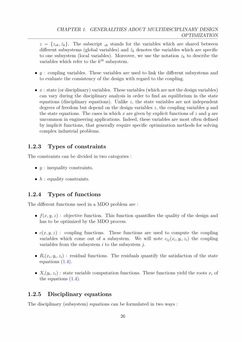
z = {zsh, zk}. The subscript sh stands for the variables which are shared betweendifferent subsystems (global variables) and zk denotes the variables which are specificto one subsystem (local variables). Moreover, we use the notation zk to describe thevariables which refer to the kth subsystem.
• y : coupling variables. These variables are used to link the different subsystems andto evaluate the consistency of the design with regard to the coupling.
• x : state (or disciplinary) variables. These variables (which are not the design variables)can vary during the disciplinary analysis in order to find an equilibrium in the stateequations (disciplinary equations). Unlike z, the state variables are not independentdegrees of freedom but depend on the design variables z, the coupling variables y andthe state equations. The cases in which x are given by explicit functions of z and y areuncommon in engineering applications. Indeed, these variables are most often definedby implicit functions, that generally require specific optimization methods for solvingcomplex industrial problems.
1.2.3 Types of constraintsThe constraints can be divided in two categories :
• g : inequality constraints,
• h : equality constraints.
1.2.4 Types of functionsThe different functions used in a MDO problem are :
• f(x, y, z) : objective function. This function quantifies the quality of the design andhas to be optimized by the MDO process.
• c(x, y, z) : coupling functions. These functions are used to compute the couplingvariables which come out of a subsystem. We will note cij(xi, yi, zi) the couplingvariables from the subsystem i to the subsystem j.
• Ri(xi, yi, zi) : residual functions. The residuals quantify the satisfaction of the stateequations (1.4).
• Xi(yi, zi) : state variable computation functions. These functions yield the roots xi ofthe equations (1.4).
1.2.5 Disciplinary equationsThe disciplinary (subsystem) equations can be formulated in two ways :
26

1.2. MATHEMATICAL FORMULATION OF THE GENERAL MDO PROBLEM
• Non-residual form (explicit):xi = Xi(yi, zi) (1.5)
In this case, the state variables can be explicitly determined from the design and cou-pling variables.
• Residual form (implicit) :Ri(xi, yi, zi) = 0 (1.4)
In this form, there is no explicit relation to determine the state variables from thedesign and coupling variables.
We can distinguish two methods for handling the disciplinary equations (Fig. 1.2) :
Disciplinary analysis
Definition 1.2.1. Given the design and coupling variables (respectively zi and yi), the dis-ciplinary analysis consists in finding the values of the state variables xi such that the state(disciplinary) equations Ri(xi, yi, zi) = 0 are satisfied.
Generally, when the disciplinary equations are expressed in the residual form, a specificsolver (e.g. a Newton algorithm) is used in order to find the roots of the equations (1.4).When the non residual-form is used, the iterative loop is not required in the subsystembecause the state variables are directly expressed from the design and coupling variables byexplicit relationships. In this case, the calculation scheme consists in sequentially evaluatingthe different relationships in order to compute the disciplinary outputs (Eq. 1.5).
Disciplinary evaluation
Definition 1.2.2. Given the design, coupling and state variables (respectively zi, yi and xi),the disciplinary evaluation consists in calculating the value of the residuals Ri(xi, yi, zi).
In this scheme, the equations (1.4) are not solved. Furthermore, the state variables xare not handled in the subsystem but are considered as inputs in the same way as z and y.The disciplinary evaluation just computes the value of Ri but does not solve the equationsRi = 0. Consequently, in case of residual form, this process takes much less computationtime than the disciplinary analysis.
As we shall see later, this dichotomy in the way to handle the disciplinary equationsis the principal difference between the All At Once and the Individual Discipline Feasibleformulations.
1.2.6 CouplingFrom the variables yi and zi coming in the subsystem i and the state variables xi, the couplingvariables which come out of the subsystem can be calculated with the coupling functionsci(xi, yi, zi). The double indexation cij(xi, yi, zi) denotes that these coupling variables are
27

CHAPTER 1. GENERALITIES ABOUT MULTIDISCIPLINARY DESIGNOPTIMIZATION
Subsystem analysisx | R (x ,y ,z )=0 or x = X (z ,y )
z , y
x
Subsystem evaluation
z , y , x
R (x ,y ,z )=?
x ,y ,z
c (x ,y ,z )
c (x ,y ,z )
DISCIPLINARY EVALUATORDISCIPLINARY ANALYZERi i
i i i i i
i i i i i
i i i
i i i i
i i i i
i i i i
i i i
c (x ,y ,z )i i i i
c (x ,y ,z )i i i i
Figure 1.2: Disciplinary analyzer and disciplinary evaluator
transmitted from the ith subsystem to the jth subsystem. The coupling is consistent whenthe set of coupling variables yi is equal to the set returned by the different coupling functions(Eq. 1.3).
1.2.7 Multidisciplinary analysisDefinition 1.2.3. The MultiDisciplinary Analysis (MDA) is a process which aims to sat-isfy the individual disciplinary feasibilities and the consistency of the couplings between thedifferent subsystems. The MDA consists in finding, for all the subsystems, the variables xiand yi such that the state equations are satisfied and the couplings are consistent.
In other words, the MDA consists in satisfying the system formed by the equations (1.3)and (1.4), as follows :{
∀i ∈ {1, · · · , n},∀j 6= i, yi = {cji(xj, yj, zj)}j∀i,∈ {1, · · · , n}, Ri(xi, yi, zi) = 0
A classical way to perform the MDA is to use the Fixed Point Iteration (FPI). The FPIgenerally consists of a loop between the different disciplinary analyses (each of them findingthe state variables x in order to make the disciplinary residuals zero). This technique requiressome properties of the coupling function and may not converge if the considered function isnot contractive [Banach, 1922]. Different numerical schemes of the MDA (Gauss-Seidel andGauss-Jacobi, etc.) are developed in details in [Keane and Nair, 2005].
1.3 Feasibility concepts in MDOWe can distinguish two feasibility concepts in MDO. These concepts are related to thefeasibility of either only one subsystem or all the subsystems.
1.3.1 Individual disciplinary feasibilityDefinition 1.3.1. A process is qualified as “individual disciplinary feasible” [Cramer et al.,1994] if at each iteration, the state equations of the different disciplines are satisfied.
28

1.4. DESCRIPTION OF THE LAUNCH VEHICLE DESIGN PROBLEM
In other words, the individual disciplinary feasibility means that we are always able tofind the values of the state variables x which satisfy the equations (1.4) (but the consistencyof the couplings is not guaranteed). Trivially, a process in which all the disciplinary equationsare in the non-residual form (Eq. 1.5) is intrinsically “individual disciplinary feasible” .
1.3.2 Multidisciplinary feasibilityDefinition 1.3.2. A process is qualified as “multidisciplinary feasible” [Cramer et al., 1994]if at each iteration, the state and coupling variables (respectively xi and yi) can be foundsuch that the “individual disciplinary feasibility” is realized and the couplings are consistent.
A problem in which a MDA is performed is a “multidisciplinary feasible” problem. In thiskind of problems, we can express the values of the state variables exclusively in function ofthe design variables : x = Xc(z) (the subscript c stands for the consistency of the coupling).Table 1.1 summarizes the level of centralization and the different degrees of feasibility of aMDO process.
Concept Process used at Variables handled Variables handledsubsystem level by the subsystems outside the subsystems
No feasibility ensured Disciplinary evaluation x,y,zIndividual disciplinary feasibility Disciplinary analysis x y,z
Multidisciplinary feasibility MDA x,y z
Table 1.1: Different feasibility concepts and corresponding involved variables
As we will see in Chapter 2, these two feasibility concepts are the principal differencebetween the Multi Discipline Feasible and the Individual Discipline Feasible formulations.
1.4 Description of the Launch Vehicle Design problemIn this section, we briefly present the Launch Vehicle Design (LVD) problem. To this end, wedescribe the different disciplines, variables and constraints involved in such a problem, andwe point out the specificities of this design problem with respect to other MDO problems.A launch vehicle is a specific vehicle which aims to put a payload in a certain orbit. Alaunch vehicle is a dynamical system which moves using rocket propulsion and involves amulti stage architecture. The different stages of the launch vehicle are jettisoned during theflight. These stages can land on Earth (e.g. the boosters), enter in the atmosphere (e.g. theintermediary stages) or remain in space (e.g. the last stage).
1.4.1 Disciplines and variablesThe Launch Vehicle Design problem is generally decomposed into the different physicaldisciplines. The classical disciplines involved in such design problems are :
• aerodynamics,• propulsion,
29
CHAPTER 1. GENERALITIES ABOUT MULTIDISCIPLINARY DESIGNOPTIMIZATION
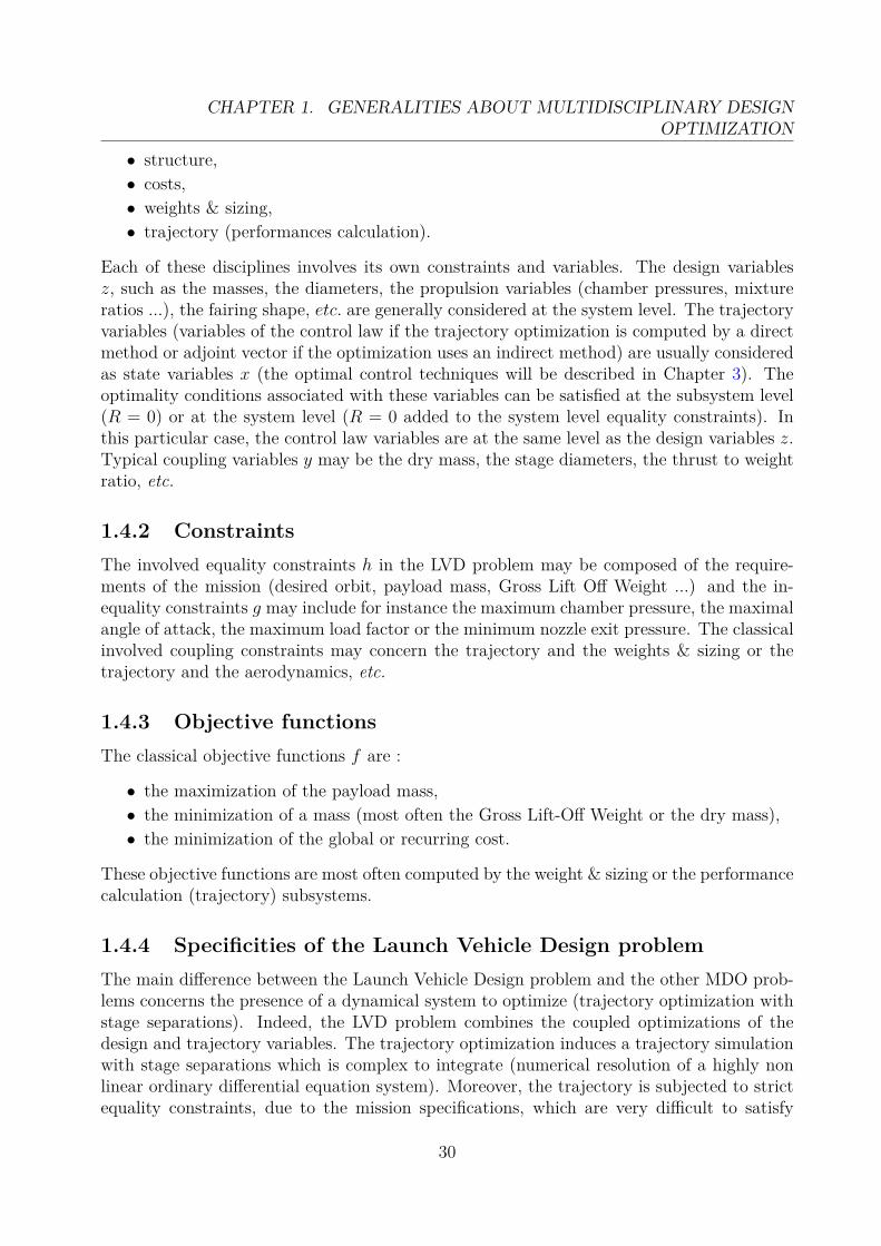
• structure,• costs,• weights & sizing,• trajectory (performances calculation).
Each of these disciplines involves its own constraints and variables. The design variablesz, such as the masses, the diameters, the propulsion variables (chamber pressures, mixtureratios ...), the fairing shape, etc. are generally considered at the system level. The trajectoryvariables (variables of the control law if the trajectory optimization is computed by a directmethod or adjoint vector if the optimization uses an indirect method) are usually consideredas state variables x (the optimal control techniques will be described in Chapter 3). Theoptimality conditions associated with these variables can be satisfied at the subsystem level(R = 0) or at the system level (R = 0 added to the system level equality constraints). Inthis particular case, the control law variables are at the same level as the design variables z.Typical coupling variables y may be the dry mass, the stage diameters, the thrust to weightratio, etc.
1.4.2 ConstraintsThe involved equality constraints h in the LVD problem may be composed of the require-ments of the mission (desired orbit, payload mass, Gross Lift Off Weight ...) and the in-equality constraints g may include for instance the maximum chamber pressure, the maximalangle of attack, the maximum load factor or the minimum nozzle exit pressure. The classicalinvolved coupling constraints may concern the trajectory and the weights & sizing or thetrajectory and the aerodynamics, etc.
1.4.3 Objective functionsThe classical objective functions f are :
• the maximization of the payload mass,• the minimization of a mass (most often the Gross Lift-Off Weight or the dry mass),• the minimization of the global or recurring cost.
These objective functions are most often computed by the weight & sizing or the performancecalculation (trajectory) subsystems.
1.4.4 Specificities of the Launch Vehicle Design problemThe main difference between the Launch Vehicle Design problem and the other MDO prob-lems concerns the presence of a dynamical system to optimize (trajectory optimization withstage separations). Indeed, the LVD problem combines the coupled optimizations of thedesign and trajectory variables. The trajectory optimization induces a trajectory simulationwith stage separations which is complex to integrate (numerical resolution of a highly nonlinear ordinary differential equation system). Moreover, the trajectory is subjected to strictequality constraints, due to the mission specifications, which are very difficult to satisfy
30

1.5. CONCLUSION
and considerably limit the feasible search domain (domain for which all the constraints aresatisfied). We will study more in details the specificities of the LVD problem when we willdescribe the application of the MDO methods in LVD in the fourth chapter of this part.
1.5 ConclusionIn this chapter, we have introduced the fundamental notions necessary to describe a MDOprocess. To this end, the general formulation of a MDO problem and the different vari-ables, functions and constraints involved in such problems have been detailed. From thedescription of the different ways to handle the disciplinary equations, the different feasibilityconcepts have been described. Finally, the requirements of the launch vehicle design and themain differences between such design problem and other MDO problems have been brieflydescribed.
The different notations and the concepts introduced in this chapter will be useful in thenext chapter which will be devoted to the general description of the main MDO formulations.We will also use these notations in the second part of this document in order to describe ourproposed MDO methods.
31


Chapter 2
Classical MDO methods
Contents2.1 Introduction . . . . . . . . . . . . . . . . . . . . . . . . . . . . . . 332.2 Single level methods . . . . . . . . . . . . . . . . . . . . . . . . . . 34
2.2.1 Multi Discipline Feasible . . . . . . . . . . . . . . . . . . . . . . . . 342.2.2 Individual Discipline Feasible . . . . . . . . . . . . . . . . . . . . . 362.2.3 All At Once . . . . . . . . . . . . . . . . . . . . . . . . . . . . . . . 38
2.3 Qualitative comparison of the single level methods . . . . . . . 392.4 Multi level methods . . . . . . . . . . . . . . . . . . . . . . . . . . 40
2.4.1 Collaborative Optimization . . . . . . . . . . . . . . . . . . . . . . 402.4.2 Modified Collaboration Optimization . . . . . . . . . . . . . . . . . 422.4.3 Concurrent SubSpace Optimization . . . . . . . . . . . . . . . . . . 442.4.4 Bi-Level Integrated Systems Synthesis . . . . . . . . . . . . . . . . 462.4.5 Analytical Target Cascading . . . . . . . . . . . . . . . . . . . . . 492.4.6 Other multi level methods . . . . . . . . . . . . . . . . . . . . . . . 51
2.5 Conclusion . . . . . . . . . . . . . . . . . . . . . . . . . . . . . . . 52
2.1 IntroductionSince the last two decades of the XXth century, a lot of MDO methods have been proposed inthe literature. Indeed, many authors such as Sobieski, Braun, Cramer, etc. have proposednew MDO formulations in order to more efficiently cope with the engineering problemsthey have to solve. This chapter is devoted to the description of the main MDO methodspresent in the literature. We can find many MDO methods which have been applied ina great number of examples. Because the study cases are different, it is difficult to com-pare these methods in order to determine which is the best. Some review articles [Ballingand Sobieszczanski-Sobieski, 1994; Alexandrov and Hussaini, 1995; Sobieszczanski-Sobieskiand Haftka, 1997; Agte et al., 2009; Tosserams et al., 2009] provide a state-of-the-art ofthe different MDO methods. The aim of this chapter is not to make an exhaustive list ofthe different MDO methods but at first to describe the main MDO methods with commonstandardized notations introduced in the first chapter. One of the goals of this part is toevaluate the applicability of the expressed methods in launch vehicle design and to bring
33

CHAPTER 2. CLASSICAL MDO METHODS
out the advantages and the drawbacks of these methods with regard to this specific problem.
This chapter is devoted to the description of the MDO methods. To this end, the chap-ter is organized as follows. In the second section, we describe the single level methods i.e.the MDO methods which only require one optimizer. The third section is devoted to thequalitative comparison of these single level methods. The fourth section concerns the de-scription of the main multi level methods (involving more than one optimizer). For each ofthe described methods, we expose at first the principle of the method, then its mathematicalformulation accompanied by an explanatory scheme, and finally we present the advantagesand drawbacks of the considered MDO method.
2.2 Single level methods
2.2.1 Multi Discipline FeasiblePrinciple
The Multi Discipline Feasible (MDF) method is the most usual MDO method. It is alsocalled “Nested Analysis and Design” (NAND), “Single NAND-NAND” (SNN) and “All-in-One”. This method is explained in [Balling and Sobieszczanski-Sobieski, 1994; Cramer et al.,1994; Kodiyalam, 1998; Allison, 2004; Gang et al., 2005]. The architecture of the MDFmethod is similar to the architecture of a classical optimization problem which involves onlyone subsystem. The main difference is that, in MDF, the subsystem is replaced by a completemultidisciplinary analysis which is performed at each iteration of the optimization process.Thus, all the subsystems are coupled in an analysis module which ensures the multidisci-plinary feasibility of the solution at each iteration (Fig. 2.1). In this formulation, the set ofdesign variables is transmitted to the analysis module. This module executes, by a dedicatedmethod (e.g. Fixed Point Iteration or Newton method), the multidisciplinary analysis of thesystem (1.3)-(1.4).
Formulation I.2 (MDF formulation)
Minimize f(Xc(z), y, z)With respect to z ∈ Z
Subject to g(Xc(z), y, z) ≤ 0 (2.1)h(Xc(z), y, z) = 0 (2.2)
Once the MDA is performed, the analysis module output vector is used by the systemlevel optimizer to compute the objective function and the constraints. The process is re-peated at each iteration. In this method, each set of found design variables is a consistentconfiguration. Furthermore, the disciplines are in charge of finding their local variables xto satisfy their own equations (1.4) (disciplinary analyzers are used). In this manner, thestate variables do not intervene in the optimization problem formulation because they aretotally handled by the disciplinary analyzers during the MDA at the subsystem level. In the
34

2.2. SINGLE LEVEL METHODS
MDF method, each found solution is multidisciplinary feasible (i.e. individual disciplinaryequations (1.4) as well as coupling equations (1.3) are satisfied). We can note that the term“multidisciplinary feasible” does not imply the satisfaction of design constraints g and h,but only the MDO ones.
Some systems do not present any feedback between the different subsystems (i.e. [Du-ranté et al., 2004], [Castellini et al., 2010]). In this case, a sequential analysis, withoutiteration, is possible and the MDF method is the most natural method to solve this kind ofproblems. Indeed, for these problems, the coupling constraints (Eq. 1.3) are automaticallysatisfied by the sequential calculation process.
For large scale (industrial) application cases, the different subsystem disciplinary analysescan be composed of groups of specialists (each of them potentially located in a different placeall over the world). In this case, the MDA becomes a very complex task and includes :
• transmission of informations between the different groups of specialists (dotted linesin Figure 2.1), and not only between computers or optimization programs,
• management requirements between and inside the different groups (because each grouppotentially converses with all the others),
• definition of each group action domain and autonomy with respect to the community(in order to ensure as much as possible the consistency of the trade-off establishments).
Subsystem 1analyzer
Subsystem ianalyzer
Subsystem nanalyzer
Multidisciplinary analysis
Optimizer
z f,g,h
x
x
x
1
i
n
min f(Xc(z),y,z)
g(Xc(z),y,z)<0
h(Xc(z),y,z)=0
R (x ,y ,z )=0or x =X (y ,z )
i i i
i i i
i
i
1iy
Figure 2.1: MDF method
35

CHAPTER 2. CLASSICAL MDO METHODS
Advantages and drawbacks of MDF
The main advantage of the MDF method is its simplicity. Indeed, a limited number of opti-mization variables is used (only the design variables z have to be handled by the optimizer)and classical disciplinary analyzers are used. The method implementation is relatively easysince the system decomposition is not required. Moreover, if the optimization process isstopped, the found solution is consistent with respect to the couplings and the individualdisciplinary feasibilities, even if it is not the optimal one.
The MDF method presents important drawbacks. Indeed, the calculation cost is veryimportant and the method does not take advantages of the couplings between the disciplinesin order to improve the optimization process, because the optimizer does not control thechoices performed by the MDA, which is considered as a black box. The calculation costis due to the MDA which has to be executed at each iteration of the optimization process.This analysis considers all the subsystems present in the MDO process (the MDF methodmodularity is very poor). Thus, when a design variable changes, all the other variables haveto be recalculated. Furthermore, a gradient-based algorithm used as the optimizer will needa full MDA whenever the derivatives required to compute the gradient or the Hessian willhave to be calculated [Kodiyalam, 1998]. Moreover, if the MDA is performed by a FPI, theMDA may not converge if the considered function is not contractive. Consequently, MDF isprincipally applicable to the optimization problems for which the different subsystems canbe quickly evaluated during the MDA or for which the MDA converges in a few iterations.
For large scale application problems (in which the subsystems are engineering teams),at each iteration, the MDA requires a lot of information transmissions and managementtasks because each group has to potentially converse with all the others. The MDA isalso responsible for defining the action domain of each specialty group (possible conflictresolutions with engineers who want to decide design and to have as much autonomy aspossible). Moreover, each group of specialists has to wait for the previous one in order toperform its task (when FPI is used), that can be very time consuming.
2.2.2 Individual Discipline FeasiblePrinciple
The Individual Discipline Feasible (IDF) method [Cramer et al., 1994; Martins and Marriage,2007], also called “Optimizer-Based-Decomposition” (OBD) [Kroo, 2004], “Single-SAND-NAND” (SSN) [Balling and Sobieszczanski-Sobieski, 1994], allows to avoid a complete mul-tidisciplinary analysis at each iteration of the design process. Like MDF, a single optimizerat the system level is used and disciplinary analysis blocks are called in the different sub-systems. The main difference between MDF and IDF is that for IDF, the optimizer is alsoresponsible for the coordination of the different subsystems and uses additional variables(coupling variables y) to ensure it. At each iteration of the optimization process, the differ-ent subsystems are individually feasible but the consistency of the couplings between themis not guaranteed. The IDF formulation of a MDO problem may be summarized as follows :
36

2.2. SINGLE LEVEL METHODS
Formulation I.3 (IDF formulation)
Minimize f(X(y, z), y, z)With respect to (y, z) ∈ Y × Z
Subject to g(X(y, z), y, z) ≤ 0 (2.3)h(X(y, z), y, z) = 0 (2.4)
∀i ∈ {1, · · · , n}, ∀j 6= i, yi = {cji(Xj(yj, zj, ), yj, zj)}j (2.5)
This method allows to break up the main problem into several subsystems. The couplingvariables (and the associate coupling equations (1.3)) are introduced in order to evaluate theconsistency of the results found by the different subsystem analyzers. In IDF, the consistencyof the solution (multidisciplinary feasibility Eq. 1.3) is not ensured at each iteration butonly at the convergence. Consequently, the IDF process should not be stopped before theconvergence is reached.This decomposition method considerably increases the number of variables handled at thesystem level but allows to improve the computational speed (parallelization is possible).Therefore, unlike the MDF method, a single analysis is performed at each iteration in thedifferent subsystems. The centralization degree of the IDF method is more important thanthe MDF one. There again, the subsystems determine their state variables (subsystemanalyzers are used).
Optimizer
Subsystem 1analyzer
x1
Subsystem nanalyzer
xn
z ,y iz ,y1 z ,yn
z,y
f, y - c, g, hmin f(X(y,z),y,z)
g(X(y,z),y,z)<0
h(X(y,z),y,z)=0
i, j=i, y ={c (x ,y ,z )} jjjii
Subsystem ianalyzer
xi
R (x ,y ,z )=0or x =X (y ,z )
i i i
i i i
f ,g , h , c iji i i
i
i
j
1 i n
Figure 2.2: IDF method
Advantages and drawbacks of IDF
If the number of coupling variables is relatively small, the IDF method is applicable andprovides results in a limited computational time. Since the principle of this method is tointroduce additional coupling variables and constraints at the system level, the number ofiterations at the system level is more important than in MDF. The optimizer has to dialogwith each disciplinary block and transmits to each of them its own coupling variables.
In return, the IDF method presents the advantage of being implementable in a network
37

CHAPTER 2. CLASSICAL MDO METHODS
(parallelization is possible). This particularity can considerably improve the efficiency ofthe method (calculation time is reduced). Furthermore, since the MDA process is removed,the internal analysis loop is broken up. In this way, if the system level optimizer requiressensitivity calculations of the ith subsystem, the other subsystems do not intervene and nocomputation time is wasted. Therefore, if an important centralization of the optimizationprocess is possible, the IDF method can be employed to effectively solve a MDO problem.
For large scale applications (for which the subsystems are composed of engineers), themanagement tasks are less important than in MDF because each group just converses withthe coordinator and not with all the others. Indeed, since the MDA is broken, the differentengineering teams have not to wait for the results of other teams, that allows to parallelizethe human tasks. However, the autonomy of the different teams is limited because the multidisciplinary feasibility is not ensured at the subsystem level, but at the system level.
2.2.3 All At OncePrinciple
The All At Once (AAO) method, also called “Single-SAND-SAND” (SSS) [Balling andSobieszczanski-Sobieski, 1994; Balling and Wilkinson, 1997] solves simultaneously the opti-mization problem and the equations of the different subsystems [Allison, 2004]. The equa-tions (2.8), (2.9) are not satisfied at each iteration of the optimization process but they haveto be at the convergence [Cramer et al., 1994] (the design configuration is consistent onlyat the convergence). In this method, the subsystem equations (residuals) are considered asequality constraints R = 0.
AAO is the most elementary MDO method. The control of the process is assigned to asystem level optimizer which aims to optimize a global objective and calls subsystem evalu-ations. The optimizer handles the design variables z, the coupling variables y and the statevariables x. At the subsystem level, the disciplinary analyzers are replaced by disciplinaryevaluators. The design and the evaluations at the subsystem and system levels are performedat the same time. Therefore, the centralization of the problem is more important than inIDF and MDF. The AAO formulation of the MDO problem can be summarized as follows :
Formulation I.4 (AAO formulation)
Minimize f(x, y, z)With respect to (x, y, z) ∈ X × Y × Z
Subject to g(x, y, z) ≤ 0 (2.6)h(x, y, z) = 0 (2.7)
∀i ∈ {1, · · · , n}, Ri(xi, yi, zi) = 0 (2.8)∀i ∈ {1, · · · , n}, ∀j 6= i, yi = {cji(xj, yj, zj)}j (2.9)
The global state vector is divided into subvectors which are distributed to each subsys-tem. The residuals R are transmitted to the global optimizer simultaneously with the other
38

2.3. QUALITATIVE COMPARISON OF THE SINGLE LEVEL METHODS
variables. Since the residuals are equal to zero only at the optimum, the multidisciplinaryand the individual disciplinary feasibilities are not ensured at the intermediary points.
Optimizer
Subsystem 1 evaluator
Subsystem i evaluator
Subsystem n evaluator
x ,y , zi i
f ,R ,c ,g ,hi i ij i i
x ,y, z
f, R, y-c, g, hmin f(x,y,z)
g(x,y,z)<0
h(x,y,z)=0
i, R (x ,y ,z )=0
i, j=i, y ={c (x ,y ,z )} jjjii
i i i
R (x ,y ,z )=?i i i
j
i
i
i
Figure 2.3: AAO method
Advantages and drawbacks of AAO
The AAO method is the less complex method to solve MDO problems because it does notmake any difference between the different involved variables which are all handled at thesame level. Nevertheless, AAO presents some drawbacks which make it inapplicable to largescale launch vehicle design problems. Indeed, in the case of problems which consider severalcomplex subsystems, the number of variables handled by the optimizer soars, that makesAAO not applicable.
In the situations for which the convergence is not achieved, the AAO method (like IDF)does not provide a feasible design. Moreover, the AAO method is difficult to implementbecause highly centralized. This method may present some robustness difficulties becausethe formulation results in a very constrained MDO problem. In relatively small problems,AAO, like IDF, is applicable and allows to parallelize calculations. Thus, the computationtime may be considerably reduced.
For large scale applications, the different groups of engineers do not perform the indi-vidual disciplinary analysis of the different subsystems but are just reduced to make sim-ple calculations with respect to the instructions given by the system level. Indeed, simplecomputations of the residuals are involved at the subsystem level, that do not require theintervention of engineering teams at this level. For this reason, the AAO method is just ap-plicable to small problems for which all the calculations can be performed by a small groupof generalist engineers.
2.3 Qualitative comparison of the single level methodsCramer et al. [Cramer et al., 1994] have performed a qualitative comparison of the MDF,IDF and AAO methods. Table (2.1) sums up this comparison and adds some considerations
39

CHAPTER 2. CLASSICAL MDO METHODS
concerning the large scale applications. In this table, the term “decision” stands for theaction on the design variables z.
AAO IDF MDFUse of traditional (engineering) No Yes Yes, couplinganalysis tools is requiredIndividual disciplinary feasibility Only at At each At eachof the solution convergence iteration iterationMultidisciplinary feasibility Only at Only at At eachof the solution convergence convergence iterationVariables handled x, y, z y, z zby the optimizerConvergence Fast Medium Slowspeed expected
- Large scale applications -Decomposition into Yes Yes Noconcurrent data processesDecomposition into Yes, but not Yes Noconcurrent human tasks judiciousAutonomy of None Small Moderateengineering teams No decision No decision No decisionat the subsystem No analysis Ind. discip. Multi discip.level analysis analysis
Table 2.1: Qualitative synthesis of the single level methods
2.4 Multi level methodsAfter having described in the previous section the three main single level MDO methods, wepresent in this section the MDO multi level methods i.e. the MDO methods which presentmore than one optimizer.
2.4.1 Collaborative OptimizationPrinciple
The Collaborative Optimization (CO) method, initially developed by Braun et al. [Braunand Kroo, 1995], is a bi level optimization method. This method has been elaborated to givemore autonomy to the different subsystems in order to satisfy the compatibility constraintsbetween the different subsystems. The optimization problem is subdivided into disciplinarysubproblems. In each subproblem, the local optimizer :
• controls its local design variables,
40
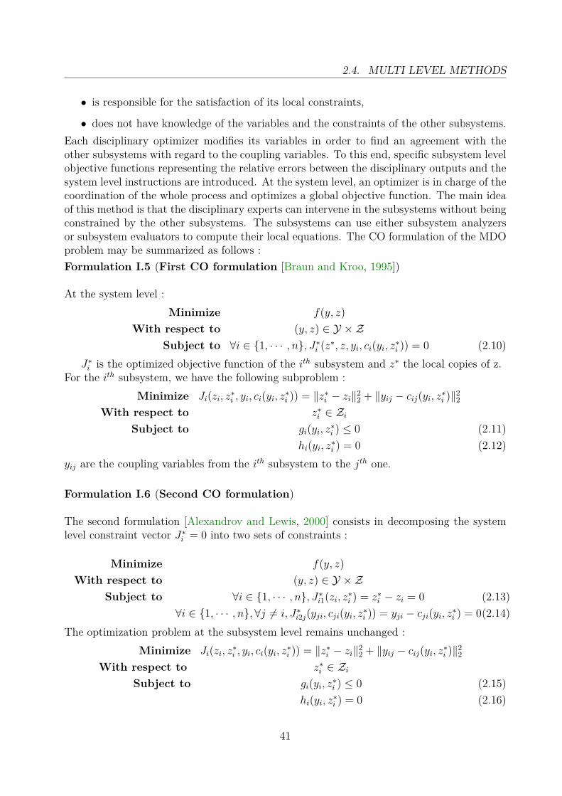
2.4. MULTI LEVEL METHODS
• is responsible for the satisfaction of its local constraints,
• does not have knowledge of the variables and the constraints of the other subsystems.Each disciplinary optimizer modifies its variables in order to find an agreement with theother subsystems with regard to the coupling variables. To this end, specific subsystem levelobjective functions representing the relative errors between the disciplinary outputs and thesystem level instructions are introduced. At the system level, an optimizer is in charge of thecoordination of the whole process and optimizes a global objective function. The main ideaof this method is that the disciplinary experts can intervene in the subsystems without beingconstrained by the other subsystems. The subsystems can use either subsystem analyzersor subsystem evaluators to compute their local equations. The CO formulation of the MDOproblem may be summarized as follows :Formulation I.5 (First CO formulation [Braun and Kroo, 1995])
At the system level :Minimize f(y, z)
With respect to (y, z) ∈ Y × ZSubject to ∀i ∈ {1, · · · , n}, J∗i (z∗, z, yi, ci(yi, z∗i )) = 0 (2.10)
J∗i is the optimized objective function of the ith subsystem and z∗ the local copies of z.For the ith subsystem, we have the following subproblem :
Minimize Ji(zi, z∗i , yi, ci(yi, z∗i )) = ‖z∗i − zi‖22 + ‖yij − cij(yi, z∗i )‖2
2
With respect to z∗i ∈ ZiSubject to gi(yi, z∗i ) ≤ 0 (2.11)
hi(yi, z∗i ) = 0 (2.12)yij are the coupling variables from the ith subsystem to the jth one.
Formulation I.6 (Second CO formulation)
The second formulation [Alexandrov and Lewis, 2000] consists in decomposing the systemlevel constraint vector J∗i = 0 into two sets of constraints :
Minimize f(y, z)With respect to (y, z) ∈ Y × Z
Subject to ∀i ∈ {1, · · · , n}, J∗i1(zi, z∗i ) = z∗i − zi = 0 (2.13)∀i ∈ {1, · · · , n},∀j 6= i, J∗i2j(yji, cji(yi, z∗i )) = yji − cji(yi, z∗i ) = 0(2.14)
The optimization problem at the subsystem level remains unchanged :Minimize Ji(zi, z∗i , yi, ci(yi, z∗i )) = ‖z∗i − zi‖2
2 + ‖yij − cij(yi, z∗i )‖22
With respect to z∗i ∈ ZiSubject to gi(yi, z∗i ) ≤ 0 (2.15)
hi(yi, z∗i ) = 0 (2.16)
41

CHAPTER 2. CLASSICAL MDO METHODS
J ,c ,g ,h
System optimizer
Subsystem 1 Subsystem i Subsystem n
z* ,yi iz* ,y1 1
z* ,yn n
z,y
Optimizer 1
Optimizer iOptimizer n
J ,c ,g ,hi i1 1 1 n n n
min f(z,y)
J*(z,z*,y,c(y,z*))=0
min J (z*,z ,y ,c (y ,z*))
g (y , z*)<0
h (y ,z*)=0
i i i i
i
i
J*
i i1 J ,c ,g ,hn
i i
i
i
i
i
i
Figure 2.4: CO method
Advantages and drawbacks of CO
CO presents significant advantages with respect to the single level optimization methods.Indeed, it is not necessary to modify the disciplinary codes in order to integrate a disciplineinto the CO optimization scheme (the modularity of the method is improved). Furthermore,CO allows to use the optimization methods that are the most adapted to each subproblem,with possible actions of disciplinary experts. This method also allows to add or to modifysome subsystems without changing the whole design process. Finally, CO is very flexible andthe subsystems calculation efficiency can be improved by using response surfaces in additionto the local optimizers [Sobieski and Kroo, 2000].
Unfortunately, practical and theoretical issues with regard to the convergence of COwhen using a sum-squared formulation for local J have been observed by some researchers[Cormier et al., 2000; Alexandrov and Lewis, 2000]. Indeed, CO seems not to be robustbecause it generates instabilities at the convergence and may fail to converge on some simpletest problems [Alexandrov and Lewis, 2000]. To overcome this difficulty, DeMiguel et al.have proposed other formulations (Inexact Penalty Decomposition, Exact Penalty Decom-position [DeMiguel and Murray, 2006], Modified Collaborative Optimization) which ensurethe equivalence of Karush-Kuhn-Tucker (KKT) conditions with respect to the initial MDOproblem. Moreover, as the number of coupling variables increases, the CO method efficiencydecreases. In other words, if the original MDO problem has a great number of couplingvariables, CO can be inefficient in terms of calculation time. Nevertheless, this approach hasbeen shown to be valid and to provide good results for some MDO problems [Braun et al.,1996].
2.4.2 Modified Collaborative OptimizationPrinciple
The Modified Collaborative Optimization (MCO) method, described in [DeMiguel and Mur-ray, 2000; DeMiguel, 2001], presents the same architecture as CO but tries to correct somedrawbacks of the CO method (e.g. non differentiability problems). MCO replaces the
42

2.4. MULTI LEVEL METHODS
quadratic penalty function used in CO by an exact form. Indeed, in order to avoid theinstabilities induced by the quadratic penalty function, MCO changes the quadratic form oflocal objective into an IDF form with adding elastic variables (si and ti) [Gill et al., 1981].Furthermore, the equality constraints at the system level are replaced by a penalty function.The MCO formulation of the MDO problem at the system level is :
Formulation I.7 (MCO formulation)
Minimize f(z, y) + wn∑i=1
J∗i (z, y)
With respect to (y, z) ∈ Y × Z
The problem formulation of the ith subsystem is :
Minimize Ji =∑
(si + ti) ≡ ‖z∗i − zi‖1 + ‖yij − cij‖1
With respect to z∗i ∈ Z∗i , si = {zsi, csi} ∈ Si, ti = {zti, cti} ∈ Ti, ri ∈ Ri
Subject to hi(yi, z∗i ) = 0 (2.17)gi(yi, z∗i ) + ri = 0 (2.18)z∗i + zsi − zti = zi (2.19)cij + csi − cti = yi (2.20)
si, ti, ri ≥ 0 (2.21)
with :
• ri : slack variables added to transform the inequality constraints g ≤ 0 in equalityones;
• (si, ti) : elastic variables [Gill et al., 1981; Boman, 1999] (si, ti=0 at the convergence);
• w : penalty coefficient (weight).
The algorithm of MCO is the same as the one of the CO method, apart from the fact thatat the subsystem level, the different optimizers have to handle the slack variables and theassociated constraints.
Advantages and drawbacks of MCO
MCO presents theoretically some advantages in comparison with the CO method. Indeed,MCO avoids instabilities of CO and aims to improve the convergence properties. As we shallsee later, MCO has been tested in a Launch Vehicle Design problem [Brown and Olds, 2006].Unfortunately, the results of this study do not allow us to conclude about the efficiency ofthis method in this specific application case.
43

CHAPTER 2. CLASSICAL MDO METHODS
System optimizer
z,y
Optimizer 1
Optimizer i
Optimizer n
J*min f(z,y) + w J* (z,y)
min J = (s +t )
h (z*,z )=0
r +g (z*,z )=0
z*+z -z =z
c +y -y =y
s ,t ,r >0
i
ii
iii
i i i
i i i i
i i i
ij
i
ij
iii
si
s t
ti
J*i
Figure 2.5: MCO method
2.4.3 Concurrent SubSpace OptimizationPrinciple
The Concurrent SubSpace Optimization (CSSO) method was formulated by Sobieszczanski-Sobieski [Sobieszczanski-Sobieski, 1988a]. This iterative method is also based on a systemdecomposition strategy which allows the subsystems to contribute independently to the op-timization process. The global problem is solved by a system level optimizer which ensuresthe coordination of the different subsystems and aims to find a compromise between thedifferent solutions proposed at the subsystem level.
Approximations of the coupling variables are used in the different subsystems in orderto determine their influence on the objective f and on the constraints g and h. With thismethod, when performing the subsystem optimizations, the effects of a variable variation inone subsystem to the constraints of the other subsystems can be determined. This methodintroduces a concept of responsibility for the constraint violation and uses cumulative con-straints [Sobieszczanski-Sobieski, 1988a], which consist in considering the partial satisfactionof a constraint in one discipline by the influences of the other disciplines. This concept ismade possible by introducing additional (coordinating) variables to the initial problem.
The approximations of the coupling variables can be performed by using neural networks[Sellar and Batill, 1996] or response surfaces [Renaud and Gabriele, 1993, 1994; Sellar et al.,1996; Wujek et al., 1996, 1997]. Other expansions of the CSSO method using approximatemodels [Rodriguez et al., 1998, 2001; Perez et al., 2002] can be found in the literature butare not developed in this document. The CSSO method uses a multidisciplinary analy-sis to coordinate the optimization process and often performs sensitivity analysis by usingthe Global Sensitivity Equation (GSE). The resolution of the GSE [Sobieszczanski-Sobieski,1990] allows to quickly obtain the total influence of the different variables to the objectivefunction. This technique will be described in Chapter 8 and Appendix C.
44

2.4. MULTI LEVEL METHODS
Formulation I.8 (CSSO formulation)
The system level optimizer solves the following problem :
Minimize f(y, zsh)With respect to zsh ∈ Zsh
Subject to g(y, zsh) ≤ 0 (2.22)h(y, zsh) = 0 (2.23)
where y represent the approximations of the coupling variables. The optimization problemof the ith subsystem can be formulated as follows :
Minimize f(yji, zsh, zi), j 6= i
With respect to zi ∈ ZiSubject to gi(yji, zsh, zi) ≤ 0 (2.24)
hi(yji, zsh, zi) = 0 (2.25)
Unlike the CO method, the shared design variables are considered as constants during theconcurrent optimizations at the subsystem level. In [Huang and Bloebaum, 2004], a CSSO-based method is presented : the Multi-Objective Pareto Concurrent SubSpace Optimization(MOPCSSO). MOPCSSO has been developed to solve multi-objective problem with a CSSOarchitecture and integrates the concept of Pareto Optimality [Pareto, 1971]. This methodallows to solve multi-objective large scale problems with a CSSO-based method.
Advantages and drawbacks of CSSO
The main characteristic of the CSSO method is the use of approximate disciplinary modelsto estimate the effects of the variables of the other disciplines and to solve the problem as adecoupled one. These approximate linearized models create a database which is used by thelocal optimizers in order to optimize the objectives and to satisfy the constraints. In thatway, CSSO method can reduce the calculation time of the optimization process. In brief, ifthe problem is relatively small and the model approximations are easy to formulate, CSSOcan be very efficient and gives solutions in a reduced calculation time.
Unfortunately, the efficiency of the CSSO method highly depends on the approximatemodels of the coupling variables. Moreover, for large scale problems, the necessary time tobuild these models can be longer than the time saved by using them. This feature can makeCSSO not enough attractive with regard to the other MDO methods.
45

CHAPTER 2. CLASSICAL MDO METHODS
Optimizer 1
Optimizer i
Optimizer n
Subsystem 1Approximation
Subsystem iApproximation
Subsystem nApproximation
CoordinationSystem optimizer
z , yi ji
min f(z,y)
g(z,y)<0
h(z,y)=0
min f (y ,z)
g (y ,z)<0
h (y ,z )=0i ji
ji
ji
Subsystem 1
Subsystem i
Subsystem n
Multidisciplinary and sensivityAnalysis
z , y
y,
Subsystem i
yji
Subsystem 1 Subsystem n
f, g, h
i
Convergence ? f opt
STOP
z 0
k
zk+1
i
i
i
z i
y i
z j
Figure 2.6: CSSO method
2.4.4 Bi-Level Integrated Systems SynthesisPrinciple
The Bi-Level Integrated System Synthesis (BLISS) method was initially proposed by Sobieszc-zanski-Sobieski [Sobieszczanski-Sobieski et al., 1998, 2000]. In this document, BLISS andBLISS2000 [Sobieszczanski-Sobieski et al., 2003] are described. BLISS2000 aims to improvethe efficiency of the classical BLISS method by using response surfaces and other approxi-mate models.
BLISS (Fig. 2.7) is an iterative multi level method which is organized into a global op-timizer at the system level and a set of disciplinary optimizers at the subsystem level. Thismethod resorts to a system analysis and subsystem analyses in order to improve the sharedand individual design variables zsh, zi. The method is based on a gradient approach andoptimizes successively the contributions of the shared and individual design variables to theobjective function.
46

2.4. MULTI LEVEL METHODS
Formulation I.9 (BLISS formulation)
At the kth iteration, the system level optimizer solves the following problem :
Given fk, zshkMinimize fk + ∂f
∂zsh∆zsh
With respect to ∆zsh
The ith subsystem solves the problem :
Given zsh, zi, yi
Minimize ∂f∂zi
∆ziWith respect to ∆zi
Subject to g(zi, zzh, yi) ≤ 0 (2.26)h(zi, zsh, yi) = 0 (2.27)
with ∆z the optimization variable increments at the current iteration. In BLISS2000, weight-ing factors w are added to structure the set of disciplinary outputs oi. Here, we denote byoutput o all the variables which come from a disciplinary box. The set of output variablescontains the coupling variables c and the state variables x which result from the subsystemoptimizations. The objective of each subsystem is to minimize a weighted sum of their out-puts, considering the global variables, the coupling variables and the weights as constants.In BLISS 2000, local optimizers are replaced by sets of response surfaces which approximatethe optimized outputs c from the inputs given by the global optimizer. All along the opti-mization process, response surfaces can be improved by adding and discarding some pointsin order to estimate the behavior of the subsystems (variables oi).Formulation I.10 (BLISS2000 formulation)
The problem at the system level can be formulated as follows :
Minimize f(z, y, w) = oj
With respect to (y, z, w) ∈ Y × Z ×WSubject to ∀i ∈ {1, · · · , n},∀j 6= i, yi = {cji}j (2.28)
For the ith local optimizer, the optimization problem is the following :
Minimize∑k
wik.oik
With respect to zi ∈ ZiSubject to gi(yi, zi) ≤ 0 (2.29)
hi(yi, zi) = 0 (2.30)
The variables zsh, y, w are considered as constants during the subsystem optimization.
47

CHAPTER 2. CLASSICAL MDO METHODS
Sub-systemOptimizer 1
Sub-systemOptimizer i
Sub-systemOptimizer n
System Optimizermin f + D(f ,z )
w.r.t. z
z ,z
Discipline 1
Discipline i
Discipline n
Multidisciplinary Analysis
y, g, h
min D(f ,z ) z
w.r.t. z
g (z ,y ,z )<0
h (z ,y ,z )=0
i
i
i i
ii i
i
{z ,z }shi 0
Convergence ?STOP
f opt
shk+1 k+1i
sh
sh
i
Variables update
Sensitivities calculation
Subsystem 1 Subsystem i Subsystem n
System
k sh
sh
shz
(*)
(*)MDA is optional and allows to have a consistent starting point
Figure 2.7: BLISS method
Advantages and drawbacks of BLISS
The main advantage of the BLISS method is to separate the system level optimization andthe optimizations of the different subsystems. Thus, the use of specific optimization toolsfor each subsystem is possible, because the disciplines are considered as black boxes bythe system level optimizer, which has the knowledge of only the outputs of the differentsubsystems.
The BLISS and BLISS2000 methods, like all the gradient-based iterative methods, requirelimits on the optimization variables. Indeed, these methods will not be able to converge if thesearch space is too large or poorly defined. Like all the processes using approximate models,the efficiency of BLISS2000 is highly dependent of the quality of the response surfaces whichapproximate the solutions of the optimization subproblems. Nevertheless, these modelscan be generated off-line by specialists who make them more stable to the design variablevariations. If the optimization subproblems are non smooth and the associate responsesurfaces have to be often redefined, BLISS2000 may provide not accurate results with anexplosion of calculation time. BLISS prefers to handle a small number of global design
48

2.4. MULTI LEVEL METHODS
variables and gives results in limited calculation time for well decomposed problems.
Subsystem i
System Optimizer
z, y, w
min w .o
w.r.t. z
g (y ,z ) < 0
h (y ,z ) = 0
Optimizer i
Subsystem i
Response surfaces i
Subsystem n
c, omin o
w.r.t z, y, w
y - c = 0
i i
ii
i i
j
Subsystem 1
i
j
Convergence?o optSTOP
Figure 2.8: BLISS2000 method
2.4.5 Analytical Target CascadingPrinciple
The Analytical Target Cascading (ATC) method, described in [Michelena et al., 1999, 2003;Kim, 2001], has been initially developed to formalize industrial product development pro-cesses. This formulation is very suitable to solve problems with a hierarchical structure.ATC is a multi level MDO method (possibly involving more than 2 levels) which hierarchi-cally propagates system and subsystem level targets through the different subsystem levels.In this formulation, the initial problem is subdivided into a set of subproblems. The spec-ified design targets are “cascaded” from the system level to the lower levels and are also“rebalanced” to the higher levels after being optimized at the lower levels.
At each level of the design process, a specific optimization problem is formulated to min-imize the errors between the level outputs and the propagated objectives, and thus to ensurethe consistency concerning the couplings between the upper and lower optimization levels.For some problems, the mathematical formulation of ATC can be similar to the CO one[Allison et al., 2005].
Let Sij be the jth subsystem of the ith optimization level, the optimization problem tosolve for this subsystem is the following :
49
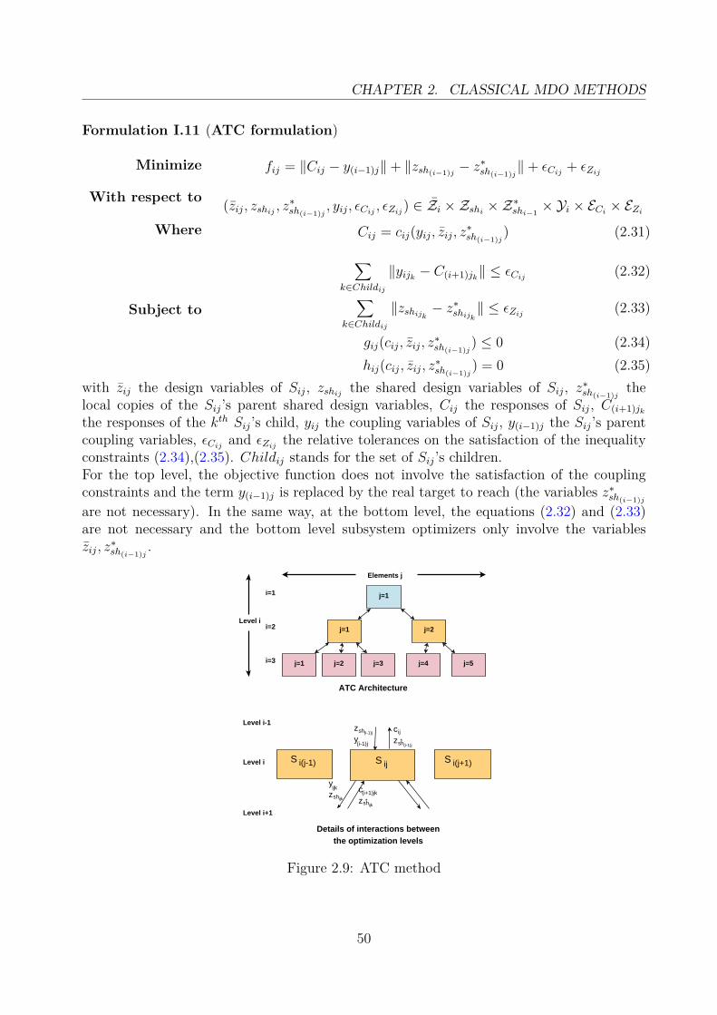
CHAPTER 2. CLASSICAL MDO METHODS
Formulation I.11 (ATC formulation)
Minimize fij = ‖Cij − y(i−1)j‖+ ‖zsh(i−1)j − z∗sh(i−1)j
‖+ εCij + εZij
With respect to (zij, zshij , z∗sh(i−1)j, yij, εCij , εZij) ∈ Zi ×Zshi ×Z∗shi−1
× Yi × ECi × EZiWhere Cij = cij(yij, zij, z∗sh(i−1)j
) (2.31)
Subject to
∑k∈Childij
‖yijk − C(i+1)jk‖ ≤ εCij (2.32)∑
k∈Childij‖zshijk − z
∗shijk‖ ≤ εZij (2.33)
gij(cij, zij, z∗sh(i−1)j) ≤ 0 (2.34)
hij(cij, zij, z∗sh(i−1)j) = 0 (2.35)
with zij the design variables of Sij, zshij the shared design variables of Sij, z∗sh(i−1)jthe
local copies of the Sij’s parent shared design variables, Cij the responses of Sij, C(i+1)jkthe responses of the kth Sij’s child, yij the coupling variables of Sij, y(i−1)j the Sij’s parentcoupling variables, εCij and εZij the relative tolerances on the satisfaction of the inequalityconstraints (2.34),(2.35). Childij stands for the set of Sij’s children.For the top level, the objective function does not involve the satisfaction of the couplingconstraints and the term y(i−1)j is replaced by the real target to reach (the variables z∗sh(i−1)j
are not necessary). In the same way, at the bottom level, the equations (2.32) and (2.33)are not necessary and the bottom level subsystem optimizers only involve the variableszij, z
∗sh(i−1)j
.
yzsh(i-1)j cij
zsh(i-1)j*
yijk
zshijk
c(i+1)jk
zshijk*
S ij
(i-1)j
Level i S i(j-1) S i(j+1)
Level i-1
Level i+1
Elements j
Level i
j=1
j=1 j=2
j=1 j=2 j=3 j=4 j=5
i=1
i=2
i=3
ATC Architecture
Details of interactions betweenthe optimization levels
Figure 2.9: ATC method
50

2.4. MULTI LEVEL METHODS
Advantages and drawbacks of ATC
ATC is a generic formulation adapted to the large scale problems which can be solved with amulti level structure. By partitioning the MDO process into a series of levels, ATC allows todistribute the complexity of the MDO problem into the different subsystems present in thedifferent optimization levels. For that reason, ATC is adapted for the MDO problem whichcan be decomposed into many small subproblems. ATC has been improved using Lagrangiancoordination [Kim et al., 2006] and has been recently adapted to non-hierarchical formulation[Tosserams et al., 2010]. Convergence proof and parallelization processes of ATC have beenproposed [Michelena et al., 2003; Han and Papalambros, 2010].
2.4.6 Other multi level methods
Some other MDO methods have been proposed in the literature. Among these, we cancite the Decomposition Based Design method [Lee and Jong, 2006], the Exact and InexactPenalty decomposition methods [DeMiguel, 2001; DeMiguel and Murray, 2006], the Dis-tributed Optimization [Tribes et al., 2005], etc. In this section, we just describe three ofthem which appear as relatively promising for the LVD application.
Discipline Interaction Variable Elimination
The Discipline Interaction Variable Elimination (DIVE), described in [Masmoudi and Parte,2006; Masmoudi et al., 2008; Auroux et al., 2009; Clement, 2009], is derived from BLISS-2000 [Agte, 2005] and aims to simplify the optimization problem by separately handlingthe global, local and coupling variables. A MDA is used to handle the couplings betweenthe different subsystems. The main characteristic of this method is to use meta-models tosimplify the optimization problem. In this method, the optimization variables set is splitup into three subsets which are optimized separately at different levels of the optimizationprocess. Firstly, the local design variables are handled using meta-models and minimizingdisciplinary objective functions, then the coupling variables are determined minimizing a L2norm on the coupling constraints. Finally the global shared variables are calculated by theglobal optimizer in order to minimize a global objective function.
Dynamic Leader Follower
The Dynamic Leader Follower (DyLeaf) method, proposed by Tava and Suzuki [Tava andSuzuki, 2003] allows to split up the optimization problem without resorting to a system leveloptimizer in order to coordinate the optimization process. In this method, derived fromthe leader-follower game, each of the k optimizers takes successively the status of leader,optimizes its disciplinary criterion and changes its local variables and the global variables.The other k − 1 optimizers (followers) optimize their own objective, modify their designlocal variables and consider the global variables as constants. During the optimization, thestatus of the leader changes as many times as necessary. A selection function is added tothe optimization problem in order to determine the optimizer which becomes the leader.
51

CHAPTER 2. CLASSICAL MDO METHODS
Multidisciplinary Design Optimization based on Independent Subspaces
The Multidisciplinary Design Optimization based on Independent Subspaces (MDOIS) [Shin,2001; Shin and Park, 2005] splits up the large system to optimize into different subsystemsand uses iteratively a multidisciplinary analysis and independent subsystem optimizations tosolve the MDO problem. This method is relatively simple compared to the other optimiza-tion methods because it does not involve complex coupling analyses. In this method, eachsubsystem optimizes its own objective and the global objective function is the summation ofthe local ones. This method does not require the use of specific sensitivity calculation tech-niques such as Global Sensitivity Equation and has been verified theoretically – satisfactionof Karush Kuhn Tucker conditions – under some assumptions (e.g. separability, no equalityconstraint at subsystem level and no intervention of coupling variables in the global objectivefunction). However, this method may get into difficulty in the case of non separable (highlycoupled) problems.
2.5 ConclusionIn this chapter, we have described the main MDO methods and their mathematical formula-tions using the unified notations presented in the previous chapter. Firstly, we have detailedthe MDO formulations which involve only one optimizer and we have exposed a qualitativecomparison of these methods. Then, we have described the formulations which present mul-tiple levels of optimization. For each of the developed formulations, we have tried to showthe advantages and the drawbacks of the considered method.
After having described the main MDO methods, the logical next step will consist incomparing them with regard to their application in the Launch Vehicle Design in order todetermine which method is the best for our current study case. This comparison will be thepurpose of the fourth chapter.
In this chapter, we have only presented MDO formulations and not the optimization algo-rithms used by these formulations. Before performing the comparison of the MDO methodsin the LVD application case, we have to describe the classical optimization algorithms usedin MDO and the main methods employed to optimize the trajectory of the launch vehicle.This is the purpose of Chapter 3.
52

Chapter 3
Optimization algorithms and optimalcontrol techniques
Contents3.1 Introduction . . . . . . . . . . . . . . . . . . . . . . . . . . . . . . 533.2 Optimization algorithms used in MDO . . . . . . . . . . . . . . 54
3.2.1 Gradient-based algorithms . . . . . . . . . . . . . . . . . . . . . . . 543.2.2 Gradient-free algorithms . . . . . . . . . . . . . . . . . . . . . . . . 55
3.3 Optimal control . . . . . . . . . . . . . . . . . . . . . . . . . . . . 623.3.1 Direct methods . . . . . . . . . . . . . . . . . . . . . . . . . . . . . 643.3.2 Indirect methods . . . . . . . . . . . . . . . . . . . . . . . . . . . . 653.3.3 Single vs multiple shooting methods . . . . . . . . . . . . . . . . . 663.3.4 Collocation methods . . . . . . . . . . . . . . . . . . . . . . . . . . 683.3.5 Dynamic Programming . . . . . . . . . . . . . . . . . . . . . . . . 69
3.4 Conclusion . . . . . . . . . . . . . . . . . . . . . . . . . . . . . . . 69
3.1 IntroductionThis chapter is devoted to the presentation of the optimization algorithms used by the MDOprocesses described in the previous chapter and the main trajectory optimization methodsemployed in LVD. The second section describes the classical optimization algorithms usedin MDO. To this end, we have chosen to make the distinction between the gradient-basedand gradient-free algorithms in order to present the optimization algorithms used in MDO.Indeed, since the Launch Vehicle Design is a complex process which often calls disciplinaryblack box functions, the sensitivity calculations may not be obtained directly. These sensitiv-ities have often to be computed through finite differences and therefore are computationallyexpensive. For this reason, the choice of using a gradient-based algorithm or not is crucialand may have important consequences on the results and the process efficiency.
Moreover, the trajectory optimization is a key point in Launch Vehicle Design becauseit is a very difficult problem to solve. Indeed, it involves a non linear differential system tointegrate, is responsible for the performance calculation and is subjected to strict equalityconstraints which highly restrain the feasible search space. The third section concerns the
53

CHAPTER 3. OPTIMIZATION ALGORITHMS AND OPTIMAL CONTROLTECHNIQUES
description of the main trajectory optimization methodologies. In this section, we describethe two main family of methods which are the direct and the indirect methods. In thischapter, since we present classical optimization techniques which are not exclusive to MDOproblems, we do not make the distinction between the different kinds of variables x, y andz.
3.2 Optimization algorithms used in MDO3.2.1 Gradient-based algorithmsThe gradient-based methods are classical optimization algorithms. Basically, these algo-rithms consist in differentiating the objective function and the constraints in order to adjustthe variables. Because there exist many optimization algorithms which are very popular andwell described in literature, we will not present them in this document. Complete descrip-tions of these algorithms can be found in [Fletcher, 1987; Nocedal and Wright, 2006; Rao,2009]. In this paragraph, we just briefly present the algorithm used in this work : the Se-quential Quadratic Programming (SQP) algorithm. For more details about this algorithm,one can consult [Gill et al., 1994; Bonnans et al., 2006; Nocedal and Wright, 2006]. The SQPalgorithm is one of the most powerful non linear programming algorithm and allows to solveconstrained differentiable optimization problems such as :
Minimize f(z)With respect to z
Subject to g(z) ≤ 0 (3.1)h(z) = 0 (3.2)
The basic idea of this algorithm is to split up the initial problem into a sequence of quadraticprogramming subproblems (QP). Each subproblem is a simplification of the initial problemusing a quadratic model of the Lagrangian function and a linearization of the constraints.Basically, in order to find the direction of descent at the iteration k, the following QP problemis solved:
Minimize L(zk, λk, µk) +∇L(zk, λk, µk)T∆z + 12∆zT∇2L(zk, λk, µk)∆z
With respect to ∆zSubject to g(zk) +∇g(zk)T∆z ≤ 0 (3.3)
h(zk) +∇h(zk)T∆z = 0 (3.4)
with L(zk, λk, µk) the Lagrangian of the initial problem, λ (respectively µ) the Lagrangemultipliers vector associated to the equality (respectively inequality) constraints and ∆z thedirection of descent. The Lagrangian of the initial problem is given by :
L(z, λ, µ) = f(z) + λTh(z) + µTg(z) (3.5)Thus, the SQP algorithm involves two nested iterative processes :• the main process, which updates the values of the real objective function and con-
straints, their gradients and the Hessian of the objective function (most often using aquasi-Newton updating method like the Broyden-Fletcher-Goldfarb-Shanno method),finds the Lagrange multipliers and checks the convergence criterion,
54

3.2. OPTIMIZATION ALGORITHMS USED IN MDO
• the QP process, which solves the quadratic programming problem and is called at eachiteration of the main process. The QP problems are solved using classical gradient-based optimization methods for constrained problem.
The basic implementation of the SQP algorithm is the following :
Algorithm 1: SQP algorithmInitialize the SQP algorithm by z0, λ0 and µ0, if possible in the vicinity of theoptimum;repeat
Approximate the problem with a linearly constrained QP problem at the current z;Solve the QP problem to obtain the descent direction ∆z∗;Compute λ∗k and µ∗k (optimized values of λk and µk);if ∆z∗ 6= 0 then
Increment the new point zk+1 = zk + αd (with α a step length parameter usedto facilitate the convergence of the algorithm and chosen to satisfy the Armijoconditions [Armijo, 1966]), λk+1 = λ∗k, µk+1 = µ∗k
until ∆z∗ = 0;
In literature, we can find several gradient-based calculation techniques (such as Post-Optimality [Braun et al., 1993], System Sensitivity Analysis [Olds, 1994], Global SensitivityEquation [Sobieszczanski-Sobieski, 1990], Local Distributed Criteria [Filatyev et al., 2009])which present some interest in a MDO framework. These algorithms will be described laterin this document.
The gradient-based algorithms present some limitations. Indeed, these algorithms requiresome differentiability properties on the objective function and on the constraints, allow tofind only local solutions, have to be initialized in the vicinity of the optimum and needrestricted bounds on the optimization variables in order to converge. Nevertheless, whenthese requirements are satisfied, the gradient-based algorithms are the fastest methods andallow to efficiently find (local) optima.
3.2.2 Gradient-free algorithmsThe gradient-free algorithms may present some interest in the MDO field because the engi-neering (industrial) simulation codes may not have been designed to provide the sensitivityinformations in an efficient manner. Moreover, these algorithms allow to work with nondifferentiable functions (and constraints) whereas the classical gradient-based algorithms re-quire some differentiability and smoothness properties of the objective and the constraints.We can find many gradient-free algorithms in literature. We have chosen to describe in thissection three of them : Nelder & Mead, Genetic Algorithm and Efficient Global Optimiza-tion.
Nelder and Mead Algorithm
The Nelder & Mead algorithm [Nelder and Mead, 1965] is one of the most used gradient-free optimization algorithms to solve non linear problems. This method is also called the
55

CHAPTER 3. OPTIMIZATION ALGORITHMS AND OPTIMAL CONTROLTECHNIQUES
non linear simplex method but is not to be confused with the linear simplex method. Thismethod involves a simplex of n dimensions and uses simple geometric transformations inorder to modify the initial simplex and to get closer to an optimum. A n−simplex is ann−dimensional polytope which is the convex hull of its n + 1 vertices. Let z1, · · · , zn+1be the n + 1 vertices of the current simplex at the ith iteration (the points are orderedaccording to the values of the objective function) and z0 the center of gravity of the n firstpoints, the different geometric operations used to modify the simplex are the following ones :Algorithm 2: Nelder & Mead algorithmStep 1 – reflection :
Compute a reflected point with respect to the following relationship :zr = z0 + α(z0 − zn+1) (3.6)
if zr is worst than zn thenGo to Step 3
elseif zr is better than the kth point (k ∈ {2, · · · , n}) then
this point is placed between zk−1 and zk;zn+1 (worst point) is not considered anymore in the current simplex
elseGo to Step 2
Step 2 – expansion :Compute an expanded point as follows :
ze = zr + β(zr − z0) (3.7)
if ze is better than zr thenReplace zn+1 by ze
elseReplace zn+1 by zr
Go to Step 1Step 3 – contraction :
Calculate the contracted point :zc = z0 + δ(z0 − zn+1) (3.8)
if zc is better than zn+1 thenreplace zn+1 by zc;Go to Step 1
elseGo to Step 4
Step 4 – shrinking :For all but the best point, replace the point by :
zi = z1 + γ(zi − z1), ∀i ∈ {2, · · · , n+ 1} (3.9)
Go to Step 1
α , β , δ and γ are the reflection, contraction, expansion and reduction parameters. Classicalvalues of these parameters are : α = β = 1 and δ = γ = 1/2.
56
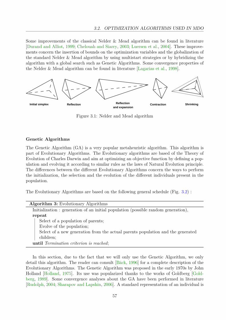
3.2. OPTIMIZATION ALGORITHMS USED IN MDO
Some improvements of the classical Nelder & Mead algorithm can be found in literature[Durand and Alliot, 1999; Chelouah and Siarry, 2003; Luersen et al., 2004]. These improve-ments concern the insertion of bounds on the optimization variables and the globalization ofthe standard Nelder & Mead algorithm by using multistart strategies or by hybridizing thealgorithm with a global search such as Genetic Algorithms. Some convergence properties ofthe Nelder & Mead algorithm can be found in literature [Lagarias et al., 1998].
Initial simplex Reflection Reflection and expansion
Contraction Shrinking
Figure 3.1: Nelder and Mead algorithm
Genetic Algorithms
The Genetic Algorithm (GA) is a very popular metaheuristic algorithm. This algorithm ispart of Evolutionary Algorithms. The Evolutionary algorithms are based of the Theory ofEvolution of Charles Darwin and aim at optimizing an objective function by defining a pop-ulation and evolving it according to similar rules as the laws of Natural Evolution principle.The differences between the different Evolutionary Algorithms concern the ways to performthe initialization, the selection and the evolution of the different individuals present in thepopulation.
The Evolutionary Algorithms are based on the following general schedule (Fig. 3.2) :
Algorithm 3: Evolutionary AlgorithmsInitialization : generation of an initial population (possible random generation),repeat
Select of a population of parents;Evolve of the population;Select of a new generation from the actual parents population and the generatedchildren;
until Termination criterion is reached;
In this section, due to the fact that we will only use the Genetic Algorithm, we onlydetail this algorithm. The reader can consult [Bäck, 1996] for a complete description of theEvolutionary Algorithms. The Genetic Algorithm was proposed in the early 1970s by JohnHolland [Holland, 1975]. Its use was popularized thanks to the works of Goldberg [Gold-berg, 1989]. Some convergence analyses about the GA have been performed in literature[Rudolph, 2004; Sharapov and Lapshin, 2006]. A standard representation of an individual is
57
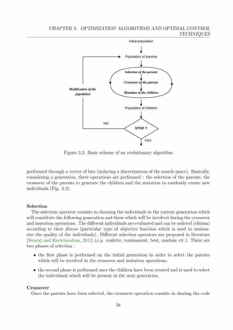
CHAPTER 3. OPTIMIZATION ALGORITHMS AND OPTIMAL CONTROLTECHNIQUES
Selection of the parents
Crossover of the parents
Mutation of the children
Population of parents
Population of children
Initial population
Modification of the
population
STOP ?NO
YES
Figure 3.2: Basic scheme of an evolutionary algorithm
performed through a vector of bits (inducing a discretization of the search space). Basically,considering a generation, three operations are performed : the selection of the parents, thecrossover of the parents to generate the children and the mutation to randomly create newindividuals (Fig. 3.2).
SelectionThe selection operator consists in choosing the individuals in the current generation which
will constitute the following generation and these which will be involved during the crossoverand mutation operations. The different individuals are evaluated and can be ordered (elitism)according to their fitness (particular type of objective function which is used to summa-rize the quality of the individuals). Different selection operators are proposed in literature[Sivaraj and Ravichandran, 2011] (e.g. roulette, tournament, best, random etc.). There aretwo phases of selection :
• the first phase is performed on the initial generation in order to select the parentswhich will be involved in the crossover and mutation operations,
• the second phase is performed once the children have been created and is used to selectthe individuals which will be present in the next generation.
CrossoverOnce the parents have been selected, the crossover operation consists in sharing the code
58

3.2. OPTIMIZATION ALGORITHMS USED IN MDO
of the parents in order to create children. Thus, the created children are new individualswhich share the characteristics of the selected parents. Since the parents have been selectedwith respect to a performance criterion, the children are expected to present good properties.There exist different ways to perform the crossover (e.g. one-point, two-point, uniform, etc.).
One-point crossover
Two-point crossover
Uniform crossover
Parents Children
Figure 3.3: Different ways to perform the crossover
MutationThe mutation operator consists in modifying the children in order to create some diversity
in the population. Basically, it consists in changing randomly one or more bit values of thecode of selected individuals (Fig. 3.4). The mutation operator allows to create new individ-uals and to optimize the criterion by performing local variations on the current population.Different ways can be found in literature in order to perform the mutation (e.g. flip bit,boundary, non-uniform, uniform, gaussian, etc.). The probability of the mutation can bestatic or can be adapted all along the optimization process.
1011001101010011001100101010101
1011001101010011001000101010101
Mutation
Figure 3.4: Example of mutation
Settings of the control parametersIn order to efficiently converge, the GA has to be tuned. Indeed, the user has to choose the
appropriate size of population and the selection, crossover and mutation control parameterscorresponding to the problem to solve. These tunings can have a great impact on the behaviorof the algorithm and the found results. For example, a too low probability of mutation maynot allow the algorithm to converge to the global optimum whereas a too high probabilitymay induce some instabilities and may lead to a total random search. In the same manner,a too low number of individuals may not allow to reach the global optimum (local minimumphenomena) whereas a too high number of individuals will increase the diversity of thepopulation, but will require an important computation time. Some authors have proposedsome guidelines to help the choice of the control parameters or some adaptive techniques to
59

CHAPTER 3. OPTIMIZATION ALGORITHMS AND OPTIMAL CONTROLTECHNIQUES
limit the intervention of the user [Srinivas and Patnaik, 1994; Eiben et al., 1999] but thechoice of the GA control parameters is a relatively problem dependent issue and the user hasoften to find the parameters which are the most appropriate to his optimization problem.
Efficient Global Optimization
The Efficient Global Optimization (EGO) algorithm [Jones et al., 1998; Sasena, 2002] usesresponse surfaces based on kriging techniques in order to propose new points to improvethe objective function. In this way, this global optimization algorithm aims to reduce thenumber of calls of the objective function and therefore aims to save calculation time. Formore details about the optimization methods using response surfaces, one can consult [Jones,2001].
From an initial database, the EGO algorithm generates a response surface using a krigingmethod, and optimizes a dedicated function called the expected improvement, which is acompromise between the predicted value of the objective function and the estimation of thelack of information in some areas of the search space, in order to propose new points ofinterest. Let us describe this algorithm more in detail.
Elaboration of the meta modelEGO is based on the kriging technique to perform the optimization. The kriging technique
[Matheron, 1963; Kleijnen, 2009] is used to approximate a function f by a gaussian process:
F (z) = mT (z)b+G(z) (3.10)
with :• m(z) : a vector of a priori regression function (constant, polynomial,etc.),• b : a vector of regression parameters to estimate from the available data,• G(z) : a centered gaussian process with a covariance k(., .) which depends on a param-
eters vector to estimate,
k(G(zi), G(zj)) = σ2GR(zi, zj) (3.11)
with :• σ2
G : the variance of the process,• R(., .) : a parametrized correlation function.
The kriging technique consists in finding the Best Linear Unbiased Predictor of F (.) [Klei-jnen, 2009]. Basically, we suppose that R(zi, zj) only depends on the relative differencebetween zi et zj (noted h). Many choices are possible to model the correlation function[Santner et al., 2003]. One of the most classical models of the correlation function is thepower exponential function :
R(h) = exp
(−
N∑k=1
∣∣∣∣∣hkθk∣∣∣∣∣pk)
(3.12)
with N the dimension of the vector z, hk the kth component of h, 0 < pk ≤ 2 and θk whichcan be estimated by maximum likelihood. pk quantifies the regularity of the function f with
60

3.2. OPTIMIZATION ALGORITHMS USED IN MDO
respect to the kth component of z and θk quantifies the sensitivity of the function f withrespect to this component. From the n points present in the database and the correspondingtrue values of the function to estimate : Zn = [z1, · · · , zn], fn = [f(z1), . . . , f(zn)], thepredictor of the mean of the gaussian process at z is given by :
F (z) = m(z)T b+ r(z)T .R−1(fn −Mb) (3.13)
with :• b = (MTR−1M)−1MTR−1fn, the maximum likelihood estimation of the regression
parameters vector b,• M = [m(z1), · · · ,m(zn)]T , the n×N matrix made up of the regression function vectors,
• r(z) = [R(z, z1), · · · , R(z, zn)]T , the vector of correlation coefficients between z andthe current database points,• Ri,j = R(zi, zj), the n×n matrix composed of the correlation coefficients of the current
database points.One of the most important advantages of the kriging model is to calculate the variance ofthe prediction error which is given by [Schonlau, 1997] :
σ2(z) = σ2G(1− r(z)TR−1r(z)) (3.14)
This characteristic is very important for the global search algorithm and is directly used inthe EGO algorithm.
True functionApproximated functionSample pointsConfidence region (95%)
Figure 3.5: Example of kriging model [Marzat et al., 2011]
Description of the optimization algorithmThe principle of EGO consists in using the kriging prediction of the (n + 1)th point in
order to get closer to the global optimum. This point is chosen by maximizing a criterionquantifying the interest of evaluating f in z, knowing Zn, fn, F (z) et σ2(z) :
zn+1 = arg maxzJ(z,Zn, fn, F (z), σ2(z)
)(3.15)
61

CHAPTER 3. OPTIMIZATION ALGORITHMS AND OPTIMAL CONTROLTECHNIQUES
A judicious choice for J is the Expected Improvement [Jones, 2001], which is defined asfollows :
EI(z) = σ(z)[uΦ(u) + φ(u)] (3.16)with :
u = fnmin − F (z)σ(z) (3.17)
fnmin = mini=1,··· ,n
{f(zi)} (3.18)
• φ : the probability density function of the normalized gaussian law N (0, 1),• Φ : a cumulative distribution function.
The optimization of the Expected Improvement allows to make a compromise between thelocal search (numerator of u) and the exploration of unchartered areas (denominator of u),that allows to perform a global optimization.Finally, the EGO algorithm is organized as follows:
Algorithm 4: Efficient Global Optimization algorithmPerform an initial (experimental) sampling of the search space (creation of initialdatabase), repeat
Given the current database, update the kriging model;Optimize the Expected Improvement function with using the kriging model, inorder to find the new point of interest;Calculate the true value of the function at this point of interest and update thedatabase.
until Termination criterion is reached;
Remark 3.2.1. Some hybrid methods, combining the heuristics and the gradient-based meth-ods have been proposed in literature. These methods aim to benefit from the efficiency of thegradient-based methods and the heuristic algorithm ability to explore large space and performglobal optimization. Most often, the employed strategy consists in firstly using a heuristicin order to find an initialization in the convergence domain of a local method which is thenapplied in order to converge quickly toward the optimum (see for example [Akhtar and Lin-shu, 2005a, 2006; Briggs et al., 2007a], etc.). Amongst the hybrid methods, we can cite theGenetic Algorithm Guided Gradient Search (GAGGS) method [Geethaikrishnan et al., 2009]which has been applied in order to optimize the trajectory of Launch Vehicles [Geethaikrish-nan et al., 2008].
3.3 Optimal controlThis section aims at giving an overview of the main optimal control techniques. A detaileddescription of the numerical methods used in the trajectory optimization can be found in[Betts, 1998; Rao, 2009]. Classically, the trajectory optimization problem consists in findingthe control law u such that :
62

3.3. OPTIMAL CONTROL
• the objective function is optimal,
• the constraints are satisfied,
• the dynamics of the system (state vector) is respected.
The dynamics of the system is commonly defined by an ordinary differential equation :
x = s(x(t), u(t), p) (3.19)
where x is the state vector, u the control law, s the state dynamics function and p the designparameters which may intervene during the trajectory integration. Initial conditions at theinitial time of the trajectory t0 are added to the problem:
h0(x(t0), u(t0), p, t0) = 0 (3.20)
In most of the cases, the initial state x(t0) is fixed (coordinates of the launching pad whenthe launch vehicle lifts off from the ground or the values of the state vector at the launchvehicle separation in the case of airborne launching) :
x(t0) = x0 (3.21)
We define also terminal conditions at the final time of the trajectory tf :
hf (x(tf ), u(tf ), p, tf ) = 0 (3.22)
The final time tf may be fixed or not. In order to avoid cumbersome notations, we supposein this part that we have only equality constraints and no path constraints. The objectivefunction is the following :
F = f(x(tf ), tf ) (3.23)We define the augmented Lagrangian :
L = [f + µThf ]tf +∫ tf
t0λT (t)[s(x(t), u(t), p)− x]dt (3.24)
where λ is the adjoint vector and µ the Lagrange multiplier vector associated to h. Then,we define the Hamiltonian :
H = λT (t)s(x(t), u(t), p) (3.25)In application of the Pontryagin Maximum Principle [Pontryagin et al., 1962], the necessaryconditions (Euler-Lagrange equations) to have an optimum (obtained by setting the firstvariation of the Lagrangian to zero) are :
λ = −HTx (3.26)
0 = HTu (3.27)
λ(tf ) = F Txt=tf
(3.28)
0 = (Ft +H)t=tf (3.29)
63

CHAPTER 3. OPTIMIZATION ALGORITHMS AND OPTIMAL CONTROLTECHNIQUES
where F stands for f + µThf and Hx (respectively Hu) is the partial derivative vector of Hwith respect to x (respectively u).Equation (3.26) is called the adjoint equation, Eq. (3.27) is the control equation, and Eq.(3.28-3.29) are the transversality equations. We can distinguish two main categories ofoptimization techniques to solve the optimization trajectory problem. These are the directand the indirect methods.
3.3.1 Direct methodsThe direct methods are the most used in the launch vehicle trajectory optimization becausethey are easy to implement and can be relatively well initialized comparatively to the indirectmethods. These methods are used in many trajectory optimization programs (e.g. Programto Optimize Simulated Trajectories - POST - [Brauer et al., 1977]). In this kind of methods,the control law is defined by a finite set of parameters upi which are handled by the optimizerin order to meet the optimality conditions. Accordingly, the control law is function of thetime and the control parameters u(upi , t). The most simple way to define u is the piece-wiselinear interpolation:
u(upi , t) =
up11 + up12t if t ∈ [t0, t1[up21 + up22t if t ∈ [t1, t2[
...upi1 + upi2t if t ∈ [ti−1, ti[
...upn1 + upn2t if t ∈ [tn−1, tn]
(3.30)
We can also use more elevated order polynomials or B-Splines [De Boor, 1978] if regularityproperties concerning the control law are required. The optimization problem is resumed asfollows :
Minimize f(x(tf ), tf )With respect to upi , i = 1, · · · , n
Subject to x(t) = s(x(t), u(upi , t), p) (3.31)hf (x(tf ), u(upi , tf ), p, tf ) = 0 (3.32)
This problem is a typical Non Linear Programming problem (NLP) and can be solved witha classical gradient-based method such as Sequential Quadratic Programming. Additionalconstraints (inequality or equality) can be added to the initial problem. One can noticethat, for this method, the calculation of the adjoint function is not necessary. Indeed, onlythe expression of the state dynamics, the control law and the initial conditions are sufficientto simulate the trajectory, compute the objective function, the final conditions and theirderivatives and so to perform the optimization. The direct methods are generally effec-tive to solve launch vehicle trajectory optimization problems. Indeed, the main advantagesof these methods are the avoidance of the adjoint vector dynamics calculation, the easyimplementation and the initialization which is easy to find. Nevertheless, these methodssuffer from several drawbacks such as a relatively low convergence speed and an important
64

3.3. OPTIMAL CONTROL
calculation cost, principally due to the sensitivity calculations when using gradient-basedalgorithms. Indeed, in most of the cases, the sensitivity calculations are performed by finitedifference approximations (Eq. 3.33 or 3.34), which imply as many trajectory simulationsas the number of parameters defining the control law. This information is required at eachiteration of the NLP.
Xupi = X(upi + δu)−X(upi)δu
(3.33)
Xupi = X(upi + δu)−X(upi − δu)2δu
(3.34)
where X stands for f or hf . Moreover, the control law found by these methods is definedby a finite set of parameters and consequently is not the real optimal one. Indeed, theperformance of the found control law is intrinsically dependent of the chosen parametricmodel. In these methods, a compromise has to be found between the complexity of thecontrol law (number of parameters) and the expected quality of the optimum.
3.3.2 Indirect methodsIn the indirect methods, the control law is not defined by a finite set of parameters anymore,but is directly deduced from the control equation (3.27) and the initial values of the stateand co-state vectors (adjoint). The aim of these methods is not to decrease the objectivefunction at each iteration but to solve the necessary conditions of optimality (PontryaginMaximum Principle [Pontryagin et al., 1962; Bryson and Y-C., 1975]) :
x(t) = Hλ(x(t), u(t), p, t), t ∈ [t0, tf ] (3.35)λ(t) = −Hx(x(t), u(t), p, t), t ∈ [t0, tf ] (3.36)u(t) = argmin
υH(x(t), υ, p, t), t ∈ [t0, tf ] (3.37)
x(t0) = x0 (3.38)λ(tf ) = F T
xt=tf(3.39)
0 = hf (x(tf ), u(tf ), p, tf ) (3.40)
The complete resolution of the problem consists of the resolution of differential system (3.35),(3.36), (3.37) according to the boundary conditions (3.38), (3.39) and (3.40). This problemis called a Two Point Boundary Value Problem (TPBVP).
Classically, this problem involves a shooting method which consists in finding the initialvalues of the adjoint vector λ(t0), the Lagrange multipliers µ and the final time tf in order tosatisfy the equations (3.22), (3.28) and(3.29). The problem amounts to solving the shootingfunction. This is commonly achieved by a Newton-Raphson method [Bonnans et al., 2006].The convergence of this process is quadratic. Moreover, in indirect methods, the control lawu is defined at each point by the Pontryagin Maximum Principle (3.27). In that way, thefound control law is a true optimum. An example of application of this method is the OP-TAX tool [Bérend and Talbot, 1996; De Biasi, 2002] developed at the CNES which employsthe indirect shooting method to solve the launch vehicle trajectory optimization problem
65

CHAPTER 3. OPTIMIZATION ALGORITHMS AND OPTIMAL CONTROLTECHNIQUES
during the exoatmospheric phase.
Find λ(t0), tf , µTo solve F T
xt=tf− λ(tf ) = 0 (3.41)
hf (x(tf ), u(tf ), p, tf ) = 0 (3.42)(Ft +H)t=tf = 0 (3.43)
Subject to x(t) = Hλ(x(t), u(t), p, t) (3.44)λ(t) = −Hx(x(t), u(t), p, t) (3.45)Hu = 0 (3.46)
Nevertheless, these methods suffer from several numerical drawbacks. Firstly, the maindifficulty of the methods is to find an initial guess of the adjoint vector in order to initializethe algorithm. Indeed, we have to be able to find an initialization that induces a point whichis relatively close to the solution at the final time in order to ensure the convergence of theNewton algorithm. Moreover, due to the integration of the trajectory, a small variation onthe initial adjoint vector can induce great repercussion at the final time and may possiblymake the trajectory diverge. Finally, for the expression of the optimality conditions, indirectmethods require the analytical differentiation of f , s and h, which may pose several problemsin case of complex physical models (e.g. aerodynamics) and limit the flexibility of the methodcomparatively to the direct methods. For that reasons, these methods are used only for theexoatmospheric phase (for which drag can be neglected).
3.3.3 Single vs multiple shooting methodsHeretofore, the described direct and indirect methods have considered the trajectory in onepiece. Indeed, from the initial conditions and the values taken by the optimization variables,the trajectory is integrated and the final conditions are returned to the optimizer in orderto evolve the optimization variables. This way to proceed may cause several problems withregard to the behavior of the optimization algorithms. The main problem is that smallvariations on variables occurring at the beginning of the trajectory may be accentuated allalong the trajectory and so may cause very harmful effects such as the trajectory divergence.This phenomenon is increased by the highly non linear nature of the dynamics function s.This aspect is crucial for the indirect methods but may have an importance for the behaviorof the direct methods as well.In order to overcome this problem, multiple shooting methods have been developed [Keller,1968]. The basic idea of these methods is to split up the trajectory into several sections. Thus,the trajectory is integrated on each elementary section, that reduces the harmful variablevariation amplification phenomenon. The values of the different initial states at the beginningof each elementary trajectory section have to be included to the initial optimization variablesset. In order to ensure the continuity between the different trajectory sections, additionalequality constraints are needed and included to the optimization problem. Let us describe
66

3.3. OPTIMAL CONTROL
the principle of multiple shooting methods in case of direct methods :The multiple shooting methods split up the initial time interval [t0 tf ] into N smaller onessuch that :
t0 < t1 < . . . < ti < . . . < tN = tf (3.47)
The values of the state vector at the beginning of each section x2, · · · , xN (and correspondingconstraints h1, · · · , hN−1) have also to be introduced and are added to the initial optimizationvariables set. Let xi(tfi) be the final state vector obtained after the integration of thetrajectory during the ith phase. The resulting set of additional constraints which have to behandled is :
h1 : x1(t1)− x2 = 0 (3.48)h2 : x2(t2)− x3 = 0 (3.49)
...hi : xi(ti)− xi+1 = 0 (3.50)
...hN−1 : xN−1(tN−1)− xN = 0 (3.51)
xi(t) is the state vector x(t) for t ∈ [ti−1, ti].The problem formulation with using the multiple shooting direct methods is the following:
Minimize f(x(tf ), tf )
With respect to upi , i = 1, · · · , Nxj, j = 1, · · · , N − 1
Subject toxi(t) = s(xi(t), u(upi , t), p), t ∈ [ti−1, ti], i = 1, · · · , N (3.52)
hj : xj(tj)− xj+1 = 0, j = 1, · · · , N − 1(3.53)hf (x(tf ), u(upN , tf ), p, tf ) = 0 (3.54)
upi denotes the set of control variables involved in the ith trajectory part.Indirect methods can also come in multiple shooting formulations [Fraser-Andrews, 1999] us-ing the same methodology. We have to note that, in this case, the additional variables includethe values of the adjoint vector at the beginning of the different parts λj, j = 1, · · · , N − 1.
Multiple shooting methods lead to an increase of N.nx of the number of optimizationvariables and constraints (with nx is the dimension of the state vector), but allow to improvethe robustness of the methods because the propagation of the non linearities is limited toeach trajectory part. State discontinuities are allowed during the optimization process.
67

CHAPTER 3. OPTIMIZATION ALGORITHMS AND OPTIMAL CONTROLTECHNIQUES
h1
h2
h3
hf
hf
t t
altitude altitude
Single shooting method Multiple shooting method
desired altitude desired altitude
Figure 3.6: Single shooting vs multiple shooting methods for a four-section trajectory
3.3.4 Collocation methods
The collocation methods [Russell and Shampine, 1972] may also be applied to the directand indirect methods and consist in discretizing the dynamics in time and replacing thedynamic equations (state and control dynamics for the direct methods, state, adjoint andcontrol dynamics for the indirect methods) by piece-wise continuous polynomials. Defectconstraints are added to the optimization problem in order to ensure the consistency betweenthe real dynamics and the approximating polynomials at the discretization points. Thus,the optimization problem results in a very large sparse NLP problem. Collocation methodsare used for example in [Hargraves and Paris, 1987; Gath and Well, 2001] to efficiently solvethe trajectory optimization problem.Let us denote by Xk(tk, xk) and U(tk, uk) the piece-wise polynomial approximations of thestate vector x in the kth interval of discretization. The problem formulation in case of directcollocation is the following :
Minimize f(XN(tN , xN), tN)
With respect to ui, i = 1, · · · , Nxj, j = 1, · · · , N
Subject toXj(tj, xj) = s(Xj(tj, xj),Uj(tj, uj), p), j = 1, · · · , N − 1(3.55)hj : Xj+1(tj, xj+1)−Xj(tj, xj) = 0, j = 1, · · · , N − 1 (3.56)
hf (XN(tN , xN),UN(tN , uN , p)) = 0 (3.57)Additional discretization points may be inserted into the N initial intervals in order to
improve the accuracy of the dynamics. The resulting NLP problem induced by the collocationmethod is very large, but the matrices of the NLP problem (Jacobian, Hessian) are sparse.In that way, exploiting the sparsity of these matrices allows to reduce the computation time.Typical approximating function used in collocation methods are the Lagrange InterpolatingPolynomials (degree D). For the kth interval, considering D collocation points between tk−1and tk, the expression of the Lagrange polynomial [Chachuat, 2006] is given by (e.g. for thecontrol law) :
68
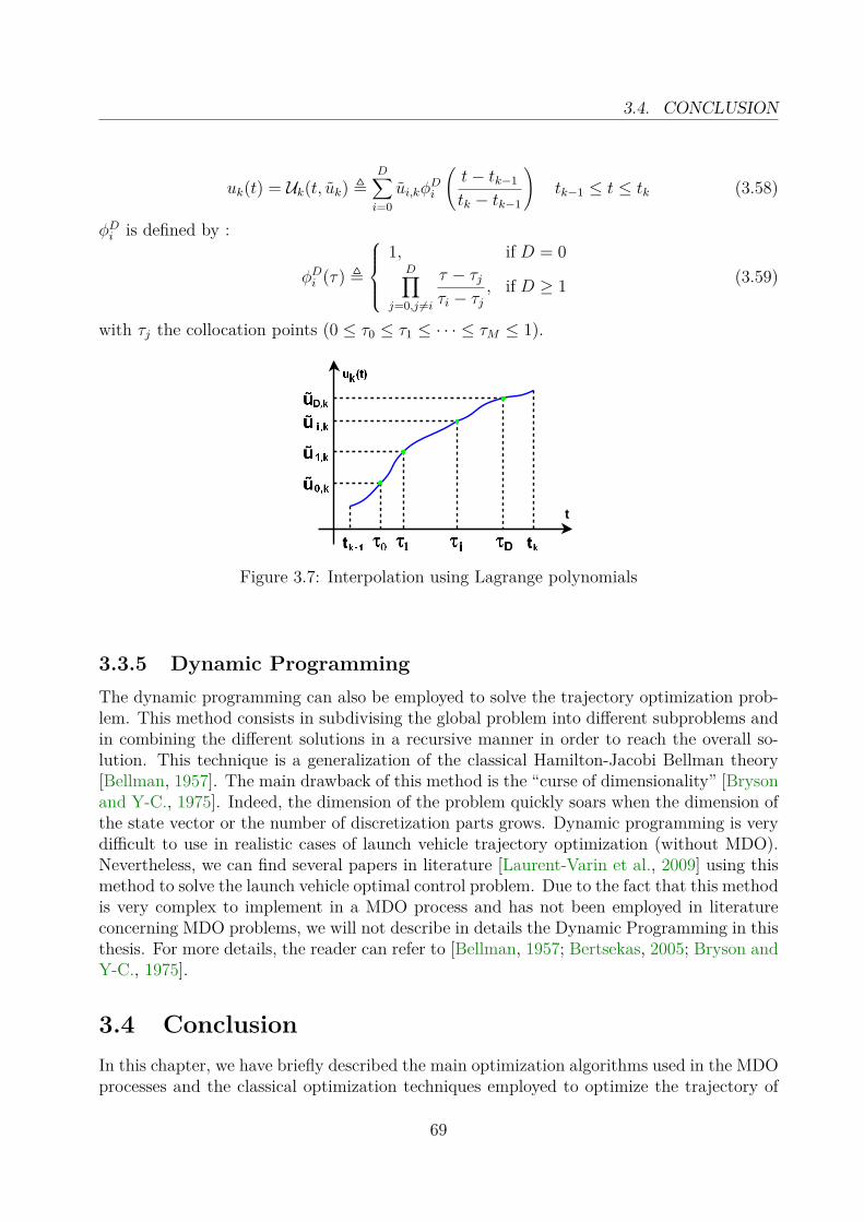
3.4. CONCLUSION
uk(t) = Uk(t, uk) ,D∑i=0
ui,kφDi
(t− tk−1
tk − tk−1
)tk−1 ≤ t ≤ tk (3.58)
φDi is defined by :
φDi (τ) ,
1, if D = 0
D∏j=0,j 6=i
τ − τjτi − τj
, if D ≥ 1 (3.59)
with τj the collocation points (0 ≤ τ0 ≤ τ1 ≤ · · · ≤ τM ≤ 1).
t
Figure 3.7: Interpolation using Lagrange polynomials
3.3.5 Dynamic ProgrammingThe dynamic programming can also be employed to solve the trajectory optimization prob-lem. This method consists in subdivising the global problem into different subproblems andin combining the different solutions in a recursive manner in order to reach the overall so-lution. This technique is a generalization of the classical Hamilton-Jacobi Bellman theory[Bellman, 1957]. The main drawback of this method is the “curse of dimensionality” [Brysonand Y-C., 1975]. Indeed, the dimension of the problem quickly soars when the dimension ofthe state vector or the number of discretization parts grows. Dynamic programming is verydifficult to use in realistic cases of launch vehicle trajectory optimization (without MDO).Nevertheless, we can find several papers in literature [Laurent-Varin et al., 2009] using thismethod to solve the launch vehicle optimal control problem. Due to the fact that this methodis very complex to implement in a MDO process and has not been employed in literatureconcerning MDO problems, we will not describe in details the Dynamic Programming in thisthesis. For more details, the reader can refer to [Bellman, 1957; Bertsekas, 2005; Bryson andY-C., 1975].
3.4 ConclusionIn this chapter, we have briefly described the main optimization algorithms used in the MDOprocesses and the classical optimization techniques employed to optimize the trajectory of
69

CHAPTER 3. OPTIMIZATION ALGORITHMS AND OPTIMAL CONTROLTECHNIQUES
the launch vehicles. From the MDO methods described in the previous chapter and theoptimization algorithms presented in the current chapter, we are now able to compare thedifferent MDO processes which have been applied in literature to solve the Launch VehicleDesign problem. This comparison is the purpose of the next chapter.Moreover, some of the optimization techniques presented in this chapter will be used inthe parts II and III when our proposed MDO methods to solve the LVD problem will bedescribed.
70

Chapter 4
Analysis of the MDO methodapplication in the Launch VehicleDesign
Contents4.1 Introduction . . . . . . . . . . . . . . . . . . . . . . . . . . . . . . 714.2 Different study cases and optimization criteria . . . . . . . . . . 72
4.2.1 MDO methods and optimization algorithms . . . . . . . . . . . . . 724.2.2 Optimization criteria and different study cases . . . . . . . . . . . 73
4.3 Trajectory handling . . . . . . . . . . . . . . . . . . . . . . . . . . 734.4 Comparison of the main MDO methods in a common applica-
tion case . . . . . . . . . . . . . . . . . . . . . . . . . . . . . . . . . 744.4.1 Presentation of the optimization problem . . . . . . . . . . . . . . 744.4.2 Comparison of AAO, MDF and CO . . . . . . . . . . . . . . . . . 744.4.3 Comparison of FPI, AAO, BLISS2000 and MCO . . . . . . . . . . 75
4.5 Comparative synthesis of the main MDO methods . . . . . . . 764.5.1 Calculation costs and convergence speed . . . . . . . . . . . . . . . 764.5.2 Considerations about optimality conditions . . . . . . . . . . . . . 764.5.3 Method deftness . . . . . . . . . . . . . . . . . . . . . . . . . . . . 77
4.6 Conclusion and ways of improvement . . . . . . . . . . . . . . . 784.6.1 Inclusion of design stability aspects in the optimization process . . 784.6.2 Trajectory optimization in the design process . . . . . . . . . . . . 794.6.3 Heuristics and gradient-based algorithms coupling . . . . . . . . . 794.6.4 Another subdivision of the optimization process . . . . . . . . . . 79
4.1 IntroductionIn literature, we can find a great number of papers dealing with the application of the MDOmethods to the Launch Vehicle Design. In order to propose some ways of improvementwith respect to the classical MDO methods used in literature, a complete analysis of theMDO methods presented in the second chapter with regard to the Launch Vehicle Designapplication is necessary. To this end, this chapter is organized as follows. In the secondsection of the chapter, we review the state-of-the-art of the MDO methods concerning the
71

CHAPTER 4. ANALYSIS OF THE MDO METHOD APPLICATION IN THE LAUNCHVEHICLE DESIGN
different study cases and the optimization criteria. This analysis will help us to determinewhich MDO method is the most employed in literature and will have to be considered inthe next part of this thesis in order to analyze the efficiency of our proposed MDO methods.The third section is devoted to the analysis of the integration of the trajectory optimizationinto the MDO processes existing in literature. In the fourth section of this chapter, wecompare the main MDO methods in a common LVD based application case using differentcriteria. This comparison will allow us to achieve a comparative synthesis of the MDOmethods, and to give in the last section some concluding remarks and to propose some waysof improvement.
4.2 Different study cases and optimization criteriaIn literature, we can find many papers dealing with the application of the MDO methods inLVD. The aim of this section is to summarize and to compare (when it possible) the differentmethods [Balesdent et al., 2011d].
4.2.1 MDO methods and optimization algorithmsThe Multi-Discipline Feasible method appears to be the most used MDO method to optimizethe design of launch vehicle. Indeed, more than 80% of the surveyed papers for this studyuse the MDF method to optimize the launch vehicle configuration. Nevertheless, we canfind several articles which apply other methods like AAO, IDF, CO, BLISS or MCO (Table4.1). The gradient-based algorithms (including Local Distributed Criteria, Post-OptimalityAnalysis, SQP, GSE, etc.) are usually preferred to the heuristic algorithms (most oftenGenetic Algorithms are used). We can also find several articles which propose hybrid algo-rithms [Akhtar and Linshu, 2005a, 2006; Briggs et al., 2007a; Geethaikrishnan et al., 2008;Rafique et al., 2009a] and combine Genetic Algorithms and gradient-based methods in orderto benefit from the advantages of these two kinds of methods.
Heuristic methods Gradient-based methods
MDF
[Akhtar and Linshu, 2005a,b, 2006][Braun et al., 1993][Braun and Kroo, 1995]
[Akhtar and Linshu, 2005a,b, 2006] [Briggs et al., 2007a][Briggs et al., 2007b][Bairstow et al., 2006] [Filatyev and Golikov, 2008; Filatyev et al., 2009]
[Bayley and Hartfield, 2007; Bayley et al., 2008] [Geethaikrishnan et al., 2008][Jodei et al., 2006][Briggs et al., 2007a,b][Collange et al., 2009, 2010] [Jodei et al., 2009][Kalden, 2007]
[Castellini et al., 2008, 2010, 2011][Delattre and Mongrard, 2007] [Kuratani et al., 2005][Lee et al., 2005a][Duranté et al., 2004, 2005][Gang et al., 2005] [Lee et al., 2005b][Moore et al., 1995]
[Kamm et al., 2007][Lee et al., 2005b][Lemaire et al., 2010] [Olds, 1992, 1994][Perrot, 2003][Qazi and Linshu, 2006][Rafique et al., 2009a,b, 2010] [Qazi and Linshu, 2006][Qu et al., 2004]
[Schoonover et al., 2000] [Rafique et al., 2009a][Tava and Suzuki, 2002][Tsuchiya and Mori, 2002, 2004][Yokoyama et al., 2005, 2007]
IDF / [Braun and Kroo, 1995]
AAO / [Braun et al., 1996][Brown and Olds, 2005][Brown and Olds, 2006][Tava and Suzuki, 2003]
CO [Gang et al., 2005]
[Braun et al., 1996][Brown and Olds, 2005, 2006]
[Cormier et al., 2000][Gang et al., 2005][Perrot, 2003]
BLISS / [Brown and Olds, 2005, 2006]MCO / [Brown and Olds, 2005, 2006]
Table 4.1: Different MDO methods applied to launch vehicle design
72
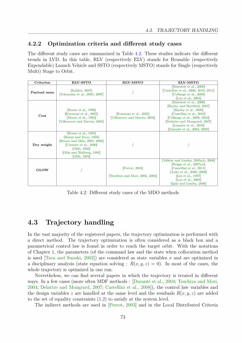
4.3. TRAJECTORY HANDLING
4.2.2 Optimization criteria and different study casesThe different study cases are summarized in Table 4.2. These studies indicate the differenttrends in LVD. In this table, RLV (respectively ELV) stands for Reusable (respectivelyExpendable) Launch Vehicle and SSTO (respectively MSTO) stands for Single (respectivelyMulti) Stage to Orbit.
Criterion RLV-SSTO RLV-MSTO ELV-MSTO
Payload mass /
[Bairstow et al., 2006][Kalden, 2007] [Castellini et al., 2008, 2010, 2011]
[Yokoyama et al., 2005, 2007] [Collange et al., 2009][Luo et al., 2004]
Cost
[Bairstow et al., 2006][Bayley and Hartfield, 2007]
[Braun et al., 1996] [Bayley et al., 2008][Kuratani et al., 2005] [Kuratani et al., 2005] [Castellini et al., 2010][Moore et al., 1995] [Villeneuve and Mavris, 2005] [Collange et al., 2009, 2010]
[Villeneuve and Mavris, 2005] [Delattre and Mongrard, 2007][Lemaire et al., 2010]
[Duranté et al., 2004, 2005]
Dry weight
[Braun et al., 1993]
/ /
[Braun and Kroo, 1995][Brown and Olds, 2005, 2006]
[Cormier et al., 2000][Olds, 1992]
[Olds and Walberg, 1993][Olds, 1994]
GLOW /
[Akhtar and Linshu, 2005a,b, 2006][Briggs et al., 2007a,b]
[Perrot, 2003] [Castellini et al., 2011][Jodei et al., 2006, 2009]
[Tsuchiya and Mori, 2002, 2004] [Liu et al., 1997][Luo et al., 2004]
[Qazi and Linshu, 2006]
Table 4.2: Different study cases of the MDO methods
4.3 Trajectory handlingIn the vast majority of the registered papers, the trajectory optimization is performed witha direct method. The trajectory optimization is often considered as a black box and aparametrical control law is found in order to reach the target orbit. With the notationsof Chapter 1, the parameters (of the command law and the state when collocation methodis used [Tava and Suzuki, 2002]) are considered as state variables x and are optimized ina disciplinary analysis (state equation solving : R(x, y, z) = 0). In most of the cases, thewhole trajectory is optimized in one run.
Nevertheless, we can find several papers in which the trajectory is treated in differentways. In a few cases (more often MDF methods : [Duranté et al., 2004; Tsuchiya and Mori,2004; Delattre and Mongrard, 2007; Castellini et al., 2008]), the control law variables andthe design variables z are handled at the same level and the residuals R(x, y, z) are addedto the set of equality constraints (1.2) to satisfy at the system level.
The indirect methods are used in [Perrot, 2003] and in the Local Distributed Criteria
73

CHAPTER 4. ANALYSIS OF THE MDO METHOD APPLICATION IN THE LAUNCHVEHICLE DESIGN
method [Filatyev and Golikov, 2008; Filatyev et al., 2009] to solve the trajectory optimiza-tion problem. In the indirect methods, an adjoint vector is used to indirectly optimize thecontrol law. In this case, the residuals R are composed of the optimality and transversalityconditions. The LDC method consists of an iterative method in which the design variableoptimization is guided by sensitivity calculations realized by an indirect approach (Post-Optimality Analysis).
The dynamic programming [Liu et al., 1997; Laurent-Varin et al., 2009] (Hamilton JacobiBellman approach) is more sporadically used in launch vehicle design because the implemen-tation of this method is not easily applicable to a complete trajectory optimization problem.
4.4 Comparison of the main MDO methods in a com-mon application case
4.4.1 Presentation of the optimization problemThe problem considered in this section is used in many papers to apply the proposed MDOmethods. This study case is the optimization of a reusable Single-Stage-To-Orbit (RLVSSTO) able to deliver 11 t of payload to the International Space Station (supposed to havea circular orbit at an altitude of 407 km and an inclination of 51.6◦). The base vehicleconfiguration is optimized using three disciplines : Performance (trajectory optimization),Propulsion and Weights & Sizing. The objective of the design process is to minimize thevehicle dry weight.
4.4.2 Comparison of AAO, MDF and COIn [Braun et al., 1996], CO, AAO and MDF are compared in the case of the SSTO launchvehicle optimization. Moreover, these methods can be compared with System SensitivityAnalysis used in [Olds, 1992, 1994] to solve an analog optimization problem.
In AAO [Braun et al., 1996], the optimizer has to handle 40 variables. Hence, for 70iterations, 2870 analysis calls are required (more than 10000 calls are required by usingMDF). Both AAO and MDF reach the same solution (within 0.05% in the dry weight).In comparison with MDF, AAO allows to considerably reduce the computation time. Thisis due to the fact that a consistent vehicle model is required only at the convergence. Sincethe disciplinary convergence is not required at each design point, the computation time isconsiderably reduced. Moreover, AAO can obtain accurate derivatives without requiringstrict convergence of the disciplinary models, that improves the process flexibility.
In the CO formulation, there are 23 design variables at the system level and 72 atthe subsystem level. At the system level, the Jacobian is obtained from the use of Post-Optimality information [Braun et al., 1993; Braun, 1996]. A SQP algorithm NPSOL [Gillet al., 1986] is used to perform the system level optimization. The objective function of theobtained solution has the same order of magnitude as the one obtained by MDF [Mooreet al., 1995]. In [Braun and Kroo, 1995], the results obtained by CO are compared with theresults obtained by AAO and MDF in [Braun et al., 1995].
From the results of this study, we can highlight two main advantages of the CO method.
74
4.4. COMPARISON OF THE MAIN MDO METHODS IN A COMMON APPLICATIONCASE
Firstly, CO is a modular method. Indeed, we can add a discipline without spending muchtime to modify the optimization process. Therefore, CO is more flexible than MDF andAAO. The second main advantage of CO is that communication requirements (betweenthe disciplines) are reduced. This is principally due to the fact that in CO, a part of theoptimization process is delegated to the different subspaces and the optimizer converses onlywith the subsystems once their optimizations are performed.
4.4.3 Comparison of FPI, AAO, BLISS2000, CO and MCOFPI, AAO, BLISS2000, CO and MCO have been compared in [Brown and Olds, 2006] in thesame realistic SSTO optimization problem. Conventional disciplines and legacy codes aretaken into account in order to be representative of classical RLV-SSTO early design studies.
Using the FPI method, each discipline handles its own variables, is subject to its ownconstraints and optimizes its part of the entire system. FPI is not a MDO method but isjust a way to solve the Multidisciplinary Analysis problem and gives a reference to comparethe methods.
In the AAO formulation, the optimizer is subject to two inequality constraints, 7 equalityconstraints and involves 13 variables. The results of this study show that AAO produces a3.94% reduction in the dry mass versus the standard FPI approach.
The BLISS method studied in [Brown and Olds, 2006] is BLISS-2000 [Sobieszczanski-Sobieski et al., 2003]. BLISS-2000 differs from BLISS-RSM [Kodiyalam, 2000; Altus, 2002]in the way the response surfaces are used. The results of this study show that BLISS isable to find an optimum which presents an improvement of 3.76% in comparison with thetraditional FPI method.
In the CO formulation, the objective of each discipline optimizer is to minimize a quadraticsum of coupling variable differences. The different disciplines handle the local copies of cou-pling variables and the objective of the global optimizer is to minimize the dry weight, subjectto the coupling consistency. The results show that CO is able to perform 4.39% reductionin the objective versus the FPI method, but provides a large convergence error.
In the MCO formulation, the objective at the system level is to optimize the weightedsum of the dry mass and the 3 local objectives of the different disciplines. The system leveloptimizer handles 9 design parameters. The study shows that in this test case, MCO ledto inconsistent results. Indeed, the resulting solution varied greatly with the value of thepenalty parameter at the system level. Due to this phenomenon, it is impossible to concludefrom this study about the efficiency of the MCO method.
Unfortunately, this study does not allow to conclude about which of the AAO, CO,BLISS2000 and MCO methods is the best in terms of the quality of the optimum, becausethe results found by these different methods are very close. Nevertheless, conclusions of thispaper show that the use of MDO methods can improve the design process (with respect toFPI). For the considered test case (which is not sufficient to provide general conclusions aboutthe methods), the study shows that AAO is very difficult to implement and is not robust(because it results in a very large and highly constrained problem) but converges quicklywith a good convergence error. CO is also difficult to implement, provides a better optimum,but with a large convergence error. BLISS2000 is the MDO method which presents the best
75

CHAPTER 4. ANALYSIS OF THE MDO METHOD APPLICATION IN THE LAUNCHVEHICLE DESIGN
performance in the considered study case because it is not very difficult to implement,converges more quickly and has a better convergence error than CO. In order to extend thiscomparison, we can compare the different methods through different qualitative criteria.This is the purpose of the following section.
4.5 Comparative synthesis of the main MDO methods
4.5.1 Calculation costs and convergence speedThe methods which involve a MultiDisciplinary Analysis are the ones that have the largestcomputation time. Indeed, the MultiDisciplinary Analysis is a very expensive process, espe-cially when it is coupled with a gradient-based method at the system level.
Decoupling the MDA considerably reduces the computation time but introduces morevariables and constraints which have to be handled by the optimizer. If the problem con-tains few disciplines, and therefore few coupling variables, IDF and AAO are the methodswhich converge fastest [Martins and Marriage, 2007]. As soon as the optimization problembecomes more complex, AAO is inapplicable because it is very difficult to implement.
Another way to improve the process efficiency is to implement a bi-level method. In thatway, the main problem can be subdivided into smaller problems and local optimizers sharethe coupling variables. The question of coupling constraints can be handled as quadraticsums of differences (CO), approximation by using response surfaces (CSSO) or by an IDFformulation (MCO). CO can considerably improve the optimization process but generatesinstabilities [DeMiguel and Murray, 2000] and an important convergence error [Brown andOlds, 2006].
The performance of CSSO in complex problems is relatively poor. Indeed, the computa-tion time used by the MDA and the generation of the approximation models can exceed thecalculation time saved by using them.
BLISS appears to have good convergence properties [Brown and Olds, 2006] and the cal-culation costs can be reduced by using approximations models (BLISS-2000, BLISS-RSM).But there again, the question of using approximate models has to be studied individually,in order to determine if it allows to save calculation time or not.
4.5.2 Considerations about optimality conditionsAmong all the methods presented in this paper, AAO is the standard MDO method becauseat the convergence, this method ensures to find a local minimum (satisfaction of the Karush-Kuhn-Tucker conditions). In principle, one should demonstrate that all the other methodsare equivalent in the satisfaction of the same KKT conditions as AAO (apart from the errorsintroduced by using approximate models). This proof is given in [Sobieszczanski-Sobieskiet al., 2003] for the BLISS method. In other words, BLISS does not introduce any other errorsthan the ones of the approximate models and of the extrapolations between the differentlevels (no theoretical errors). Nevertheless, the BLISS2000 method is subjected to convexityand response surfaces errors. Using the implicit function theorem [Kudryavtsev, 2001], thesatisfaction of the KKT conditions of the single-level methods such as MDF and IDF can alsobe proved. All the methods including an iterative scheme in the optimization process (BLISS,
76

4.5. COMPARATIVE SYNTHESIS OF THE MAIN MDO METHODS
CSSO, etc.) and requiring intrinsically sensitivity calculations need convexity properties ofthe MDO problem to solve. This characteristic is a key difference with respect to otherMDO methods (e.g. MDF, IDF, CO, etc.) which allow to employ heuristics such as GA,and consequently do not require strict convexity of the problem.
4.5.3 Method deftnessRobustness to initialization
In terms of robustness to initialization, defined here as the ability to converge to an optimumfrom a large initialization domain, AAO seems to be the worst method. Indeed, since allthe variables and all the constraints are handled by a single optimizer, AAO needs to beinitialized in the vicinity of the optimum to converge. Generally, in case of formulationswhich use approximate models, the robustness of the methods is correlated with the qualityof the models and a particular effort has to be made on the generation of these models.
Applicability to large scale systems
The heavily centralized formulations are difficult to apply with large scale systems. Indeed,because the optimizer handles a lot of coupling variables, these methods are difficult to im-plement in case of large scale systems and have poor convergence properties. In that way,AAO appears to be inapplicable in large scale problems.
CO seems to perform well for only a low number of coupling variables. BLISS, consider-ing disciplines as black boxes, is applicable to large scale systems without difficulty, even ifsystem analyses are required because they can be performed in parallel. If the disciplinarymodels are not too complex, CSSO is also applicable in large scale systems, but its efficiencyis dependent on the generated approximate models.
Concerning the application of the MDO methods in an industrial context (when engi-neering teams intervene), the single-level methods are difficult to use because they are notadapted to the organization of the industrial structures. Moreover, these methods give verysmall autonomy to the engineering teams which have no decision power on the design andonly provide disciplinary analyses.
Contrariwise, the multi-level methods (such as CO, CSSO, BLISS, etc.) can distributethe disciplinary optimizations to speciality engineering teams and furthermore are moreadapted to industrial problems. However, the efficiency of CSSO is to be put in perspectivebecause, in this formulation, the different subsystems require the approximations of the othersubsystem coupling influences.
Adaptability and implementation difficulty
Since a lot of complex disciplines are taken into account in the launch vehicle optimizationprocess, the time needed to integrate modifications is an important criterion to compare thedifferent MDO methods. The bi-level methods (BLISS, CO, CSSO, MCO) seem to be moreadaptable to a variation of the number of disciplines. For example, comparative studiesin LVD [Braun et al., 1996] show that the modification time of CO is 75% less than thestandard approach one and 66% less than the AAO one. In BLISS, since the disciplines are
77

CHAPTER 4. ANALYSIS OF THE MDO METHOD APPLICATION IN THE LAUNCHVEHICLE DESIGN
considered as black boxes, the global optimizer does not intervene in the black boxes andadding a discipline does not change the process architecture.
The implementation difficulty of the CSSO method is heavily dependent on the disci-plinary models. There again, since approximate models have to be generated in CSSO, avery complex discipline can be approximated by non smooth models which provide instabil-ities and consume a lot of computation time.
Another important criterion which has to be taken into account is the different methodadaptability when the disciplinary models or the application case change (e.g. moving froma Single-Stage-To-Orbit launch vehicle to a Two-Stage-To-Orbit, minimizing the dry massinstead of maximizing the payload mass, etc.). MDF requires a global modification everytime the design process changes, because all the disciplines are interlinked with the MDA.IDF and AAO are more flexible because each discipline evolves independently from theothers. However, these methods are specific to an application case and when this casechanges, all the process can be reorganized.
There again, the bi level methods present some advantages with respect to the single levelmethods. Indeed, these methods (especially CO and BLISS) are generic at the subsystemlevel (black boxes for the system level) and the whole design process has not to be revisedwhen a disciplinary model changes. This point is not true for CSSO because for a givensubsystem, the influences of the other subsystem behaviors have to be approximated. ForCO and MCO, because the different subsystems optimize a quadratic sum or relative errors, achange in the system level objective does not imply any modification at the subsystem level.For BLISS2000, the adaptability of the method to a modification of the global objectivefunction is ensured by the weighting factors, which can evolve all along the optimizationprocess.
4.6 Conclusion and ways of improvementIn the light of this study, we identify several ways of improvement relating to the use ofMDO methods in the specific problem of launch vehicle design.
4.6.1 Inclusion of design stability aspects in the optimization pro-cess
The design stability aspect, defined here as the insensitivity to uncertainties associatedwith both design parameters and design models, is a key factor in LVD. This particularityespecially takes sense in early phase studies, where simplified models are employed (e.g. instructure discipline, finite element codes are often replaced by simplified relationships).
From this point of view, it appears essential that this aspect has to figure as an objectiveof the optimization process [Du and Chen, 2002]. Indeed, to make sure that the processgoes smoothly, it would be interesting to insert a stability indicator, in order to help thedesigner to evaluate the quality of the solution found by the optimization process. In caseof the use of gradient-based algorithms, the design stability with respect to the constraintscan be evaluated by the Lagrange multipliers, which can be used to quantify the variation
78

4.6. CONCLUSION AND WAYS OF IMPROVEMENT
of the objective function with respect to a violation of saturated constraints.
4.6.2 Trajectory optimization in the design processThe launch vehicle design optimization is heavily coupled to the optimal trajectory calcula-tion. Indeed, the entire process is dependent of the results of the trajectory optimization, inwhich the requirements of the mission intervene.
Almost all examples in literature use a direct shooting method to optimize the launchvehicle trajectory. This choice is principally due to the fact that in the direct method, theinitialization of the parameters is easier to find than in the indirect method. Nevertheless,the direct method only provides suboptimal solutions.
The real optimal solution is given by the indirect shooting method [Bryson and Y-C.,1975; Bryson, 1999]. This method is more complex to implement but gives precious in-formations about the convergence, i.e. about the ability of the proposed launch vehicleconfiguration to reach the specifications of the mission. These informations (adjoint vectorand sensitivity of the objective with regard to the parameters) could be exploited in theglobal optimization process (the optimality conditions would be integrated in the systemlevel equality constraints h = 0), in order to change the design parameters z and the statevariables x. These considerations could improve the efficiency of the optimization process(like in the LDC method [Filatyev and Golikov, 2008; Filatyev et al., 2009]).
4.6.3 Heuristics and gradient-based algorithms couplingIn order to have a robust (to starting points), efficient and global optimization process,coupling evolutionary and gradient-based algorithms at all the optimization levels may bean interesting way of improvement. Indeed, a lot of synergisms could emanate from thecoupling of these two types of methods in the MDO process, like in the GAGGS method[Geethaikrishnan et al., 2008]. With the evolutionary algorithms, the process could ex-plore the entire design space, and therefore avoid the local optima phenomena. By usinggradient-method algorithms, the efficiency of the method could be considerably improved,and sensitivity informations could be exploited by the evolutionary algorithms in order tobring the population to optimal solutions.
4.6.4 Another subdivision of the optimization processAll the examples in literature consider a subdivision of the problem into the disciplines suchas propulsion, structure, performance calculation, etc. The trajectory optimization is con-sidered as a standard discipline. In order to improve the adaptability and the flexibilityof the optimization process, a subdivision into a stage-wise decomposition (instead of thedecomposition into the different disciplines) could place the trajectory optimization at theroot of the optimization process. This kind of decomposition could provide good results ina MDO context. Indeed, the optimization process would be subdivided in as many sub-systems as the number of stages. Each subsystem would regroup the different disciplineswhich intervene in the stage design and these subsystems would be piloted by the trajectoryoptimization (optimal control, maybe by indirect shooting method). Such a decomposition
79

CHAPTER 4. ANALYSIS OF THE MDO METHOD APPLICATION IN THE LAUNCHVEHICLE DESIGN
could be handled by a multi-level process (e.g. a collaborative method).
Following the previous study, we have chosen to work on the elaboration of new MDO for-mulations using a transversal subdivision of the LVD process in order to place the trajectoryat the center of the optimization process (Part II). Moreover, we want to develop a dedicatedoptimization strategy, which aims at coupling heuristics and gradient-based algorithms, inorder to improve the robustness of the design process (Part III).
80

Part II
Multidisciplinary DesignOptimization formulations using a
stage-wise decomposition
81

Chapter 5
Presentation of the stage-wisedecomposition formulations
Contents5.1 Introduction . . . . . . . . . . . . . . . . . . . . . . . . . . . . . . 835.2 Decomposition of the problem and identification of the couplings 85
5.2.1 Definition of the launch vehicle design problem . . . . . . . . . . . 855.2.2 Decomposition of the state vector dynamics . . . . . . . . . . . . . 875.2.3 Determination of the coupling variables . . . . . . . . . . . . . . . 885.2.4 Proposition of the optimization strategy . . . . . . . . . . . . . . . 89
5.3 Stage-wise decomposition formulations . . . . . . . . . . . . . . 915.3.1 First formulation . . . . . . . . . . . . . . . . . . . . . . . . . . . . 915.3.2 Second formulation . . . . . . . . . . . . . . . . . . . . . . . . . . . 935.3.3 Third formulation . . . . . . . . . . . . . . . . . . . . . . . . . . . 955.3.4 Fourth formulation . . . . . . . . . . . . . . . . . . . . . . . . . . . 96
5.4 Conclusion . . . . . . . . . . . . . . . . . . . . . . . . . . . . . . . 98
5.1 IntroductionThis part is devoted to the description of the stage-wise decomposition formulations. One ofthe main concluding remarks of the previous part concerns the transversal reorganization ofthe optimization process. Indeed, it emerged from the analysis of the MDO methods appliedto the LVD problem that a decomposition according to the different stages instead of the dif-ferent disciplines – which is classically performed in literature – could improve the efficiencyof the MDO process. To this end, we propose in this part different formulations exploitingthe decomposition of the optimization process into the different flight phases. In these for-mulations, the subsystems are not the disciplines anymore but are composed of the differentstage optimizations. Each stage gathers all the disciplines and is optimized separately. Theglobal trajectory is decomposed into elementary flight phases which are optimized duringthe stage optimizations.
83
CHAPTER 5. PRESENTATION OF THE STAGE-WISE DECOMPOSITIONFORMULATIONS
The decomposition into the flight phases has already been applied to optimize the tra-jectory of launch vehicles [Beltracchi, 1992; Rahn and Schöttle, 1994; Ledsinger and Olds,2002; Perrot, 2003]. The existing methods in literature consist in optimizing separately thedifferent flight phases in order to split up the original optimization problem into smallerones. These methods have been applied to optimize either the trajectory only or the tra-jectory and a small number of design variables (most often the propellant masses). Thisdecomposition has been used to optimize the trajectory of expendable [Beltracchi, 1992] andreusable launch vehicles [Rahn and Schöttle, 1994; Ledsinger and Olds, 2002; Perrot, 2003].
In [Beltracchi, 1992], a decomposition process is proposed to solve the all-up trajectoryoptimization problem concerning a booster and an upper stage in order to deliver a maximalpayload into a target orbit. The optimizations of the booster and the upper stage trajec-tories are performed separately and are coordinated through the definition of a park orbitbetween the two subsystems. The optimization strategy is an iterative process between theoptimizations of two subsystem trajectories and a system level coordinator, and sensitivitycalculations are transmitted from the subsystem to the system levels in order to improvethe optimization process. The results of this study show that the solution obtained by theproposed decomposition strategy is valid and can be a good guess for a traditional optimiza-tion considering simultaneously all the optimization variables, which presents an importantcalculation time (and may fail) when initialized with a point which is not in the vicinity ofan optimum.
In [Rahn and Schöttle, 1994], the optimization of branching trajectories of a reusabletwo-stage-to-orbit launch vehicle is solved (Sänger-type mission). The optimization processhandles the trajectory variables and the propellant masses of the different stages. The pro-posed strategy involves a system level optimizer to coordinate the orbiter and booster flightphases through the definition of a staging point. This study allows to show the capabilityof the flight phase decomposition to optimize the trajectory and a few mass variables. Nev-ertheless, the problem treated in this paper does not perform a complete multidisciplinaryoptimization and does not consider all the design variables and disciplines other than thetrajectory and the propellant mass definition (no disciplinary couplings).
In [Ledsinger and Olds, 2002], FPI, CO and two formulations of IDF are compared in theoptimization of branching trajectories of a fully reusable two-stage launch vehicle. The coor-dination of the different branches is performed through the handling of a staging point at thesystem level. This paper shows that the use of MDO methods associated to the flight phasedecomposition allows to transform the non hierarchical initial problem to a hierarchical oneand find a better optimum than using the classical engineering method (manual iterationwhich involves a loop between the sequential optimizations of the different branches). Nev-ertheless, CO appears to be more computationally expensive than the other used methodsfor this problem (Kistler K-1 problem).
In [Perrot, 2003], a FPI, a hybrid MDF which presents a MDA and a sub-optimizationat the subsystem level, and a collaborative approach which once again optimizes indepen-dently the different stages at a subsystem level and coordinates them at a system level viaa staging point, are compared in the trajectory optimization problem by using direct andindirect methods. As in [Ledsinger and Olds, 2002], a FPI method, which considers theoptimization problem as a loop between the optimizations of the different flight phases iscompared to the MDF method. Unfortunately, the results obtained for the collaborative ap-
84

5.2. DECOMPOSITION OF THE PROBLEM AND IDENTIFICATION OF THECOUPLINGS
proach are not shown. Nevertheless, this study shows that using the MDF method presentssome benefits with respect to FPI which presents a lack of consistency of the results (noconvergence towards the identified optimum whereas the MDO method allows to convergein a few system-level iterations).
All these studies are mainly focused on the trajectory optimization, involving the tra-jectory variables (with occasionally a few design parameters concerning the masses e.g. thepropellant mass) and do not consider all the disciplinary design variables and the induceddisciplinary couplings. The trajectory optimization of expendable launch vehicles presentsthe same characteristics as the RLV trajectory. Indeed, the trajectory can also be decom-posed into the different flight phases which correspond to the flights of the different stages.In this part, we use the flight phase decomposition in order to perform the complete mul-tidisciplinary design optimization of expendable launch vehicles. We do consider not onlythe trajectory but all the different disciplines present in the MDO problem (and inducedcouplings).
This part is organized in three chapters. In the first chapter, we present the differentstage-wise decomposition formulations. This chapter is based on the launch vehicle trajec-tory analysis in order to describe the different proposed MDO formulations. We first detailthe initial launch vehicle design problem, then we identify the different couplings betweenthe subsystems and finally we propose four different ways to handle these couplings. Thesecond chapter is devoted to the description of the application case. We describe the dif-ferent disciplines, variables and constraints. The second part of this chapter concerns theapplication of the proposed formulations to the detailed application case. The last chapterdeals with the theoretical and numerical comparisons of the different formulations.
5.2 Decomposition of the problem and identification ofthe couplings
In order to formally describe the proposed stage-wise decomposition formulations, we firstdefine the launch vehicle design problem. Then, we analyze the launch vehicle state vectordynamics in order to identify the couplings between the different flight phases. This analysisserves us to propose four formulations using the stage-wise decomposition to solve the launchvehicle design problem.
5.2.1 Definition of the launch vehicle design problemUsing the classical notations defined in the previous part, the launch vehicle design opti-mization problem can be formulated as follows :
85

CHAPTER 5. PRESENTATION OF THE STAGE-WISE DECOMPOSITIONFORMULATIONS
Formulation II.1
Minimize f(zd1 , · · · , zdi , · · · , zdn , y0)With respect to y0, z = {zdk , zck}, k = 1, · · · , n
Subject to gk(zdk , zck , y0, x) ≤ 0 (5.1)hk(xf ) = 0 (5.2)
c(zdk , zck , y0, x) = 0 (5.3)x = s(zdk , zck , y0, x) (5.4)
with :
• f : objective function. In LVD, the objective function is often a mass (e.g. minimumlift off mass, maximum payload mass) or a cost criterion.
• zd : design variables. These variables are the disciplinary optimization variables whichtake part in the definition of the objective function (e.g. propellant masses, diameters,pressures, etc.).
• zc : control variables. These variables allow to define the control law of the launchvehicle. These variables define the trajectory of the launch vehicle and intervene in theconstraints definition.
• y0 : initial coupling variables. These variables are used in the standard LVD prob-lem definition in order to link the different disciplines (e.g. coupling concerning themaximal load factor between the trajectory and the mass budget disciplines).
• g : inequality constraints. These constraints can be trajectory (e.g. maximal angle ofattack, mechanical and thermal loads) or design constraints (e.g. maximal nozzle exitdiameter).
• h : equality constraints. In LVD, the equality constraints often deal with the satis-faction of the mission requirements. These equality constraints are most often verydifficult to satisfy and considerably limit the feasible search domain definition.
• c : initial coupling constraints. These coupling constraints are used to ensure theconsistency of the couplings defined by the initial coupling variables y0.
• x : state vector. The state vector is used to simulate the trajectory of the launchvehicle. xf stands for the final value of x.
• s : dynamics of the state vector. These functions describe an ordinary differentialequation system which allows to define the evolution of the state vector x all along thetrajectory.
• n : number of stages.
86

5.2. DECOMPOSITION OF THE PROBLEM AND IDENTIFICATION OF THECOUPLINGS
5.2.2 Decomposition of the state vector dynamicsFor an expendable launch vehicle, the global trajectory is composed of the different stageflight phases, linked by stage separations inducing non continuous variations of the statevector (mass jettisonings). Each stage presents its own design and control variables, con-straints and dynamics functions. The dynamics of the launch vehicle state vector can bedecomposed according the different stage flight phases as follows (Fig 5.1) :
x = x1, t ∈ [0, tf1 ],...
x = xi, t ∈ [tfi−1 , tfi ],...
x = xn, t ∈ [tfn−1 , tf ].
and, {x1 = s1(zd1 , z
′d2 , · · · , z
′dn , zc1 , y0, x1) (5.5)
...xi = si(zdi , z′di+1
, · · · , z′dn , zci , y0, xi)ui0 = ui−1(tfi−1)xi0 = xi−1(tfi−1)
(5.6)(5.7)(5.8)
...xn = sn(zdn , zcn , y0, xn)un0 = un−1(tfn−1)xn0 = xn−1(tfn−1)
(5.9)(5.10)(5.11)
with :• tfi : final time of the ith flight phase,
• u(zc, t) : control law,
• xi0 (respectively ui0): initial state vector (respectively control law vector) of the ithflight phase,
• xi(tfi) (respectively ui(tfi)) : final state vector (respectively control law vector) of ithflight phase,
• z′di : design variables of the ith stage which play a part in the dynamics of other stageflight phases (e.g. all the diameters of the different stages play a part in the dynamicsof the first stage through drag calculation). z′di are defined by :
z′di = {zdij ∈ zdi |∃k 6= i,∃(zdk , zck , y0, xk),∇zdijsk(zdk , zck , y0, xk) 6= 0} (5.12)
87

CHAPTER 5. PRESENTATION OF THE STAGE-WISE DECOMPOSITIONFORMULATIONS
Time
Velocity
Flight phase 1
Flight phase i-1
Flight phase i
Flight phase n-1
Flight phase n
Figure 5.1: Decomposition of the state vector dynamics
In order to be consistent all along the trajectory, the state vector and the control lawhave to be continuous at the stage separations (except for the masses). For that purpose,the equations (5.7-5.8) and (5.10-5.11) are required.
Remark 5.2.1. The mass is a particular state variable because for multi stage launch ve-hicles, its dynamics presents discontinuities at the stage separations. The continuity of thecontrol law is not always required during the trajectory. Indeed, the control law can be dis-continuous in the exoatmospheric phases or if the control concerns the thrust. Nevertheless,in this study, we maintain the continuity of the control law during the whole trajectory.
Remark 5.2.2. Given a stage, only the design variables of the upper stages intervene in itsflight phase.
Indeed, when the ith stage begins its flight phase, all the k underneath stages (k < i)have been jettisoned and thus do not take part in the flight of the ith stage which explainsthe absence of the z′dk,k<i in the equations of the (5.5,5.6,5.9).
5.2.3 Determination of the coupling variablesThe different differential systems present some couplings which have to be handled. Thesecouplings come in addition to the initial couplings y0 and are due to the subdivision into thedifferent flight phases. All the couplings are represented by the underlined variables in thefollowing equations.
88

5.2. DECOMPOSITION OF THE PROBLEM AND IDENTIFICATION OF THECOUPLINGS
{x1 = s1(zd1 , z
′d2 , · · · , z
′dn , zc1 , y0, x1) (5.13)
...
xi = si(zdi , z′di+1
, · · · , z′dn , zci , y0, xi)
ui0 = ui−1(tfi−1)xi0 = xi−1(tfi−1)
(5.14)
(5.15)(5.16)
...
xn = sn(zdn , zcn , yn, xn)un0 = un−1(tfn−1)xn0 = xn−1(tfn−1)
(5.17)(5.18)(5.19)
The couplings symbolize the influence of the variables y0 and z′di on the stage dynamics andthe consistency of the differential system integrations (values of the state vector and thecontrol law at the initial and final times of the flight phases).
5.2.4 Proposition of the optimization strategy
Henceforth, we describe the case of the minimization of the Gross-Lift-Off-Weight (GLOW)which is a standard study case in Launch Vehicle Design, as described in Table 4.2 (Chapter4). With a few modifications, the formulation of the MDO problem can be applied in thecase of payload maximization [Balesdent et al., 2010b, 2011e] or cost minimization.
In the case of GLOW minimization, the global mass is defined as the sum of the differentstage masses and the mass of the upper composite (composed of the payload, the payloadadaptor and the fairing). Thus, the objective function can be decomposed as follows :
min(f) ≡ min(f1) +min(f2) + · · ·+min(fi) + · · ·+min(fn) + fupper composite (5.20)
where fi stands for the mass of the ith stage (the upper composite is supposed to be fixed).Using the stage-wise decomposition strategy, we can propose the following optimizationscheme :
89

CHAPTER 5. PRESENTATION OF THE STAGE-WISE DECOMPOSITIONFORMULATIONS
min(f)=⇒
min(f1(zd1 , y0))
x1 = s1(zd1 , z
′d2 , · · · , z
′dn , zc1 , y0, x1)
g1(zd1 , z′d2 , · · · , z
′dn , zc1 , y0, x1) ≤ 0
c(zd1 , z′d2 , · · · , z
′dn , zc1 , y0, x1) = 0
...
min(fi(zdi , y0))
xi = si(zdi , z′di+1, · · · , z′dn , zci , y0, xi)
xi0 = xi−1(tfi−1)ui0 = ui−1(tfi−1)gi(zdi , z′di+1
, · · · , z′dn , zci , y0, xi) ≤ 0c(zdi , z′di+1, · · · , z′dn , zci , y0, xi) = 0...
min(fn(zdn , y0))
xn = sn(zdn , zcn , y0, xn)xn0 = xn−1(tfn−1)un0 = un−1(tfn−1)gn(zdn , zcn , y0, xn) ≤ 0c(zdn , zcn , y0, xn) = 0hn(xn(tfn)) = 0
In order to decouple the different optimizations, we have to introduce additional couplingvariables and corresponding constraints, which relate to the junctions of the initial and finalconditions of the flight phases :
y = {xkf , ukf , y0}, k = 1, · · · , (n− 1) (5.21)
where y0 are the coupling variables of the initial problem and y the coupling variables of theproposed methodology. For simplification reasons, xkf (respectively ukf ) stands for xk(tfk)(respectively uk(tfk)). Therefore, a possible optimization strategy consists in splitting upthe optimization process into two levels, with a subsystem level in charge of performingthe n optimizations corresponding to the n subsystems and a system level which aims tocoordinate the subsystem optimizations, i.e. which handles the shared variables, couplingvariables and coupling constraints.We note {zdk} = {{zdk}{z
′dk}, the design variables of the subsystem k which do not play a
part in the optimization of other flight phases and zsh =n⋃i=1
z′di the shared design variables.
Moreover, we denote by zk all the variables (design and control) which play a part only inthe kth flight phase. Thus, we have the following notations :
zdk = z′dk ∪ zdk (5.22)zk = zdk ∪ zck (5.23)
zsh =n⋃i=1
z′di (5.24)
90
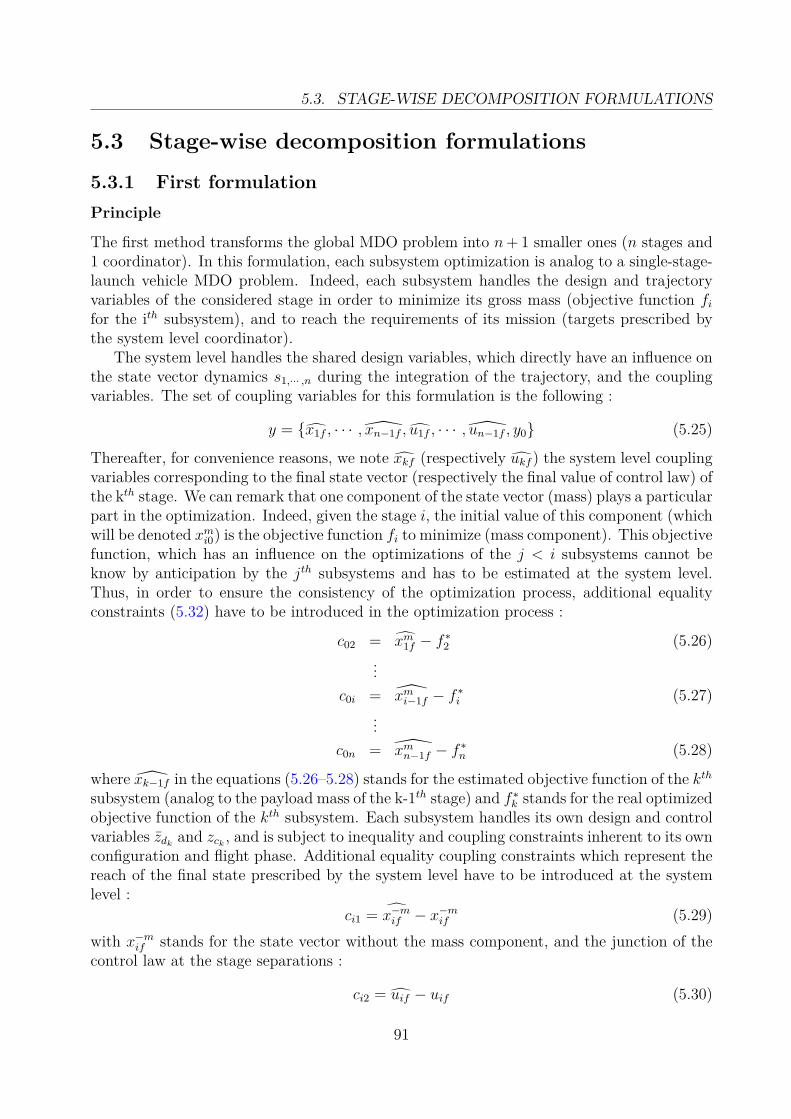
5.3. STAGE-WISE DECOMPOSITION FORMULATIONS
5.3 Stage-wise decomposition formulations
5.3.1 First formulationPrinciple
The first method transforms the global MDO problem into n+ 1 smaller ones (n stages and1 coordinator). In this formulation, each subsystem optimization is analog to a single-stage-launch vehicle MDO problem. Indeed, each subsystem handles the design and trajectoryvariables of the considered stage in order to minimize its gross mass (objective function fifor the ith subsystem), and to reach the requirements of its mission (targets prescribed bythe system level coordinator).
The system level handles the shared design variables, which directly have an influence onthe state vector dynamics s1,··· ,n during the integration of the trajectory, and the couplingvariables. The set of coupling variables for this formulation is the following :
y = {x1f , · · · , xn−1f , u1f , · · · , un−1f , y0} (5.25)
Thereafter, for convenience reasons, we note xkf (respectively ukf ) the system level couplingvariables corresponding to the final state vector (respectively the final value of control law) ofthe kth stage. We can remark that one component of the state vector (mass) plays a particularpart in the optimization. Indeed, given the stage i, the initial value of this component (whichwill be denoted xmi0) is the objective function fi to minimize (mass component). This objectivefunction, which has an influence on the optimizations of the j < i subsystems cannot beknow by anticipation by the jth subsystems and has to be estimated at the system level.Thus, in order to ensure the consistency of the optimization process, additional equalityconstraints (5.32) have to be introduced in the optimization process :
c02 = xm1f − f ∗2 (5.26)...
c0i = xmi−1f − f ∗i (5.27)...
c0n = xmn−1f − f ∗n (5.28)
where xk−1f in the equations (5.26–5.28) stands for the estimated objective function of the kthsubsystem (analog to the payload mass of the k-1th stage) and f ∗k stands for the real optimizedobjective function of the kth subsystem. Each subsystem handles its own design and controlvariables zdk and zck , and is subject to inequality and coupling constraints inherent to its ownconfiguration and flight phase. Additional equality coupling constraints which represent thereach of the final state prescribed by the system level have to be introduced at the systemlevel :
ci1 = x−mif − x−mif (5.29)with x−mif stands for the state vector without the mass component, and the junction of thecontrol law at the stage separations :
ci2 = uif − uif (5.30)
91

CHAPTER 5. PRESENTATION OF THE STAGE-WISE DECOMPOSITIONFORMULATIONS
In the equations (5.29-5.30), xif (respectively uif ) is the (real) ith final state vector (respec-tively control law) calculated at the subsystem level thanks to the integration of the ith stagetrajectory whereas xif (resp. uif ) is the final state vector (resp. control law) extracted fromy (Eq. 5.21). For the last stage, ci (Eq. 5.36) are replaced by the equality constraints hi(Eq. 5.34) symbolizing the mission requirements and there is no coupling constraint aboutthe control law.Thus, the coupling constraints (Eq. 5.29 and 5.30) ensure the consistency of the optimiza-tion process with respect to the integration of the trajectory (continuity of the dynamics Eq.5.4). The formulation of the optimization process is the following :
Formulation II.2At the system level :
Minimize f =n∑i=1
f ∗i (zsh, y) +Mupper composite
With respect to zsh, y
Subject to g0(zsh, y) ≤ 0 (5.31)c0(zsh, y) = 0 (5.32)
At the subsystem level (for the ith stage) :
Given zsh, y
Minimize fi(zdi , zsh, y)With respect to zdi , zci
Subject to gi(zdi , zsh, zci , y, xi) ≤ 0 (5.33)hi(xif ) = 0 (5.34)
ci(xif , uif , y) = 0 (5.35)c(zdi , zsh, zci , y, xi) = 0 (5.36)xi = si(zdi , zsh, zci , y, xi) (5.37)
where Eq. (5.34) are only considered for i = n and Eq. (5.35) for i 6= n.
Remarks concerning the first formulation
The first formulation allows to reduce the MDO problem to the coordination of n smallerones. Indeed, the ratio between the dimension of each subsystem problem with respect tothe global MDO problem dimension is approximatively 1/n. Moreover, by decomposing thetrajectory into n smaller parts corresponding to the flights of the stages, this formulationallows to break up the propagation of the perturbations all along the trajectory and thusto satisfy more easily the equality constraints. For these reasons, we may expect a betterbehavior of the global optimization process for the formulation 1 with respect to the initialMDF formulation (Form. II.1).
The possible drawback of the first formulation is the coupling constraints (5.32) at thesystem-level. Indeed, in this formulation, the convergence of the different subsystems and the
92

5.3. STAGE-WISE DECOMPOSITION FORMULATIONS
satisfaction of the system level equality constraints are not correlated. A possible improve-ment of this formulation consists therefore in reorganizing the subsystem optimizations inorder to correlate the system level equality constraint satisfaction with the subsystem conver-gence i.e. to find a formulation in which the subsystem convergence implies the satisfactionof the system level coupling constraints. This is the purpose of the second formulation.
5.3.2 Second formulationPrinciple
The second formulation applies the technique of Collaborative Optimization [Braun et al.,1996] to the stage-wise decomposition. Indeed, the different subsystems do not aim at min-imizing the stage masses anymore but expect to reach the targets prescribed by the systemlevel coordinator.
In this formulation, the objective function at the system level remains unchanged. Here,the subsystems do not aim to optimize fi,i=1,··· ,n but have to minimize quadratic sumsJi,i=1,··· ,n of relative differences with respect to the coupling variables specified at the systemlevel. The minimization of these quadratic sums replaces the satisfaction of the equalityconstraints at the subsystem level (Eq. 5.29, 5.30, 5.35).On the other hand, the n− 1 equality constraints (Eq. 5.26–5.28) are replaced by n equalityconstraints (Eq. 5.41–5.43) which concern the convergence of the different subsystems. Theset of coupling variables for this formulation is the following :
y = {xm10, x1f , · · · , xn−1f , u1f , · · · , un−1f , y0} (5.38)
An additional variable xm10, which stands for the launch vehicle mass at the beginning of thefirst flight phase has to be added to the optimization problem. This variable is used in thefirst stage objective function formulation.
Remark 5.3.1. In the original Collaborative Optimization formulation [Braun, 1996], thesystem level handles all the optimization variables and the different subsystems only han-dle local copies of the corresponding design variables in order to minimize their objectivefunction. The proposed second formulation differs from CO in the repartition of the designvariables. Indeed, in the second formulation, the different subsystems do not handle localcopies of the design variables but deal with the variables corresponding to the configurationand the trajectory of the stages. In the same way, the system level optimizer does not handleall the design variables but only the shared and coupling variables. Nevertheless, the secondformulation uses the CO formulation to define the subsystem level objective function and thesystem level coupling constraints.
The formulation of the optimization process is the following :
93

CHAPTER 5. PRESENTATION OF THE STAGE-WISE DECOMPOSITIONFORMULATIONS
Formulation II.3At the system level :
Minimize f =n∑i=1
f ∗i (zsh, y) +Mupper composite
With respect to zsh, y
Subject to g0(zsh, y) ≤ 0 (5.39)c0(zsh, y) = 0 (5.40)
with :
c01 = J∗1 (5.41)...
c0i = J∗i (5.42)...
c0n = J∗n (5.43)
At the subsystem level (for the ith stage) :
Given zsh, y
Minimize Ji(zdi , zsh, zci , y) =∑j 6=m
xjif − xjifΠj
2
+(uif − uif
U
)2
+xmi0 − xmi−1f
M
2
With respect to zdi , zciSubject to gi(zdi , zsh, zci , y, xi) ≤ 0 (5.44)
c(zdi , zsh, zci , y, xi) = 0 (5.45)xi = si(zdi , zsh, zci , y, xi) (5.46)
with Πj, U and M : different normalization coefficients on the objective function at thesubsystem level which are used to enhance the behavior of the optimization process. Fori = 1, we have xmi−1f = xm10, for i = n,
(uif−uif
U
)2is not considered in the objective function
and xjif − xif are the orbit injection conditions.
Remarks concerning the second formulation
The main advantage of the second formulation with respect to the first one is the improve-ment of the satisfaction of the system level coupling constraints by the modification of thedifferent subsystem objective functions. Indeed, in this formulation, the convergence of thesubsystems implies the satisfaction of the system level objective function. A second advan-tage of this formulation is the avoidance of the equality constraints h and ci at the subsystemlevel. This is due to the inclusion of these constraints into the penalized objective function.On the other hand, this formulation increases the number of coupling variables (insertion
94

5.3. STAGE-WISE DECOMPOSITION FORMULATIONS
of the estimated mass of the first stage into the coupling variables set) and the couplingconstraints (n coupling constraints instead of n− 1 for the first formulation).
In the first and second formulations, the system level aims to coordinate the optimizationprocess. To this end, these formulations require equality constraints at the system level. Evenif the second formulation improves the global behavior of the optimization process, these twoproposed formulations may cause some numerical difficulties during the optimization (e.g.difficulty to satisfy the constraints, search spaces of valid solutions are very restricted).For this reason, an alternative formulation is proposed, in order to get rid of the equalityconstraints (Eq. 5.32 and 5.40).
5.3.3 Third formulationPrinciple
The aim of the third formulation is to avoid the coupling equality constraints at the system-level. The equality constraints at the system level of the first formulation concern theestimation of the optimized masses f ∗i found during the different subsystem optimizations,in order to ensure the consistency of the optimization process. We can notice that the ithsubsystem requires only the estimations of fj,j>i. Thus, an iterative handling of the fi maybe considered at the subsystem level in order to remove the coupling equality constraints atthe system level. For that purpose, the different stages are optimized from the uppermostto the lowest stages, and once a stage optimization is performed, the optimized mass of theconsidered stage is transmitted to the lower subsystem which can begin its own optimization.In this formulation, the use of the coupling variables xmif is not necessary anymore. Thus,the search space at the system level is reduced by n− 1 dimensions. The coupling variableset used in the third formulation is the following :
y = {x−m1f , · · · , x−mn−1f , u1f , · · · , un−1f , y0} (5.47)The problem formulation of the different subsystems is the same as in the first formulation :each subsystem aims at minimizing its own mass and at satisfying its equality and inequalityconstraints. The only difference between the first and third formulations at the subsystemlevel concerns the way to perform the different subsystem optimizations. For the first formu-lation, the different subsystem optimizations can be performed independently. This is nottrue for the third formulation (non hierarchical process).
The optimization process is the following :
Formulation II.4At the system level :
Minimize f =n∑i=1
f ∗i (zsh, y) +Mupper composite
With respect to zsh, y
Subject to g0(zsh, y) ≤ 0 (5.48)
95
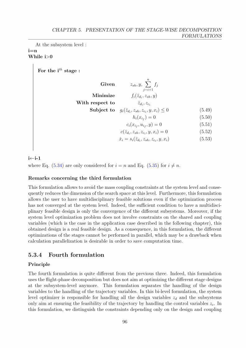
CHAPTER 5. PRESENTATION OF THE STAGE-WISE DECOMPOSITIONFORMULATIONS
At the subsystem level :i=nWhile i>0
For the ith stage :
Given zsh, y,n∑
j=i+1fj
Minimize fi(zdi , zsh, y)With respect to zdi , zci
Subject to gi(zdi , zsh, zci , y, xi) ≤ 0 (5.49)hi(xif ) = 0 (5.50)
ci(xif , uif , y) = 0 (5.51)c(zdi , zsh, zci , y, xi) = 0 (5.52)xi = si(zdi , zsh, zci , y, xi) (5.53)
i←i-1where Eq. (5.34) are only considered for i = n and Eq. (5.35) for i 6= n.
Remarks concerning the third formulation
This formulation allows to avoid the mass coupling constraints at the system level and conse-quently reduces the dimension of the search space at this level. Furthermore, this formulationallows the user to have multidisciplinary feasible solutions even if the optimization processhas not converged at the system level. Indeed, the sufficient condition to have a multidisci-plinary feasible design is only the convergence of the different subsystems. Moreover, if thesystem level optimization problem does not involve constraints on the shared and couplingvariables (which is the case in the application case described in the following chapter), thisobtained design is a real feasible design. As a consequence, in this formulation, the differentoptimizations of the stages cannot be performed in parallel, which may be a drawback whencalculation parallelization is desirable in order to save computation time.
5.3.4 Fourth formulationPrinciple
The fourth formulation is quite different from the previous three. Indeed, this formulationuses the flight-phase decomposition but does not aim at optimizing the different stage designsat the subsystem-level anymore. This formulation separates the handling of the designvariables to the handling of the trajectory variables. In this bi-level formulation, the systemlevel optimizer is responsible for handling all the design variables zd and the subsystemsonly aim at ensuring the feasibility of the trajectory by handling the control variables zc. Inthis formulation, we distinguish the constraints depending only on the design and coupling
96

5.3. STAGE-WISE DECOMPOSITION FORMULATIONS
variables gd0 from the ones depending on the trajectory gci. In the same manner, cj standsfor the coupling constraints on the state vector whereas c are the coupling constraints of theinitial problem. The coupling variable set at the system level is the same as in the thirdformulation. With the same notations, the fourth formulation is the following:Formulation II.5At the system level :
Minimize f =n∑i=1
fi(zsh, zdi , y) +Mupper composite
With respect to zsh, zdi , y, i = 1, · · · , nSubject to gd0(zsh, zdi , y) ≤ 0 (5.54)
c0(xif , uif , y) = 0, i = 1, · · · , n (5.55)
c0 is a constraint vector composed of the Ji, in the same manner as in the second formu-lation. At the subsystem level (for the ith stage) :
Minimize Ji =∑j 6=m
cij(xjif , uif , y)Πj
2
With respect to zciSubject to gci(zsh, zdi , zci , y, xi) ≤ 0 (5.56)
c(zdi , zsh, zci , y, xi) = 0 (5.57)xi = si(zdi , zsh, zci , y, xi) (5.58)
where cij stands for (xjif − xjif ) and (uif − uif ) and for i=n, Jn =
∑j 6=m
(hj(xjnf )
Πj
)2
.
Remarks concerning the fourth formulation
The fourth formulation is different from the previous three in the way the coupling constraintsare handled. Indeed, this formulation introduces the decomposition between the design andcontrol variables and splits up only the trajectory into the different parts. In this manner,this method mixes a MDF formulation with a multiple shooting method in which the differentparts of the trajectory are not only simulated but also optimized separately. This formulationis a compromise between the MDF formulation (in which all the optimization variables arehandled at the system level) and the three first formulations (in which the system levelhandles the least number of optimization variables as possible).
Remark 5.3.2. The fourth formulation can be also described within the IDF paradigm. In-deed, since the subsystems just aim at satisfying the equations (5.55), these can be consideredas disciplinary analyzers (see definition 1.2.1). In this case, the control variables zci can beconsidered as state variables and the cij are just residuals to cancel under some constraints.
Table 5.1 surveys the different characteristics of the formulations.
97
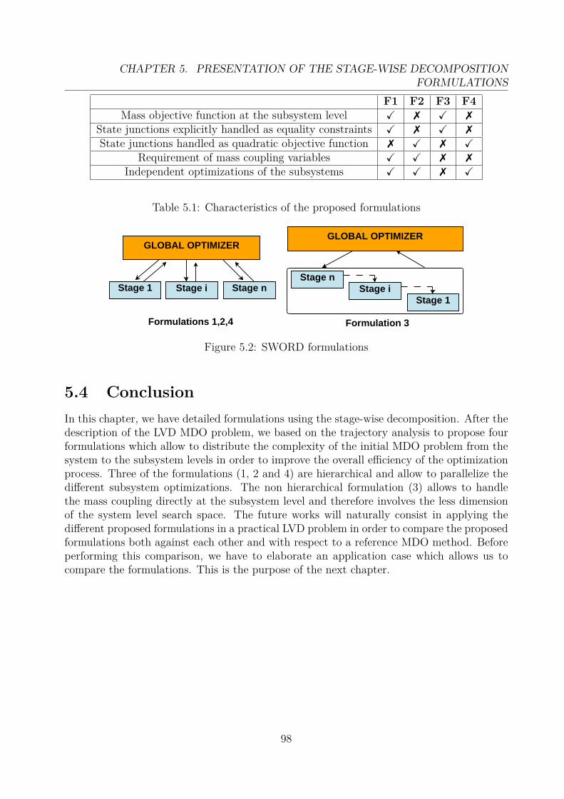
CHAPTER 5. PRESENTATION OF THE STAGE-WISE DECOMPOSITIONFORMULATIONS
F1 F2 F3 F4Mass objective function at the subsystem level X 7 X 7
State junctions explicitly handled as equality constraints X 7 X 7
State junctions handled as quadratic objective function 7 X 7 XRequirement of mass coupling variables X X 7 7
Independent optimizations of the subsystems X X 7 X
Table 5.1: Characteristics of the proposed formulations
GLOBAL OPTIMIZER
Stage i Stage nStage 1
GLOBAL OPTIMIZER
Stage nStage i
Stage 1
Formulations 1,2,4 Formulation 3
Figure 5.2: SWORD formulations
5.4 ConclusionIn this chapter, we have detailed formulations using the stage-wise decomposition. After thedescription of the LVD MDO problem, we based on the trajectory analysis to propose fourformulations which allow to distribute the complexity of the initial MDO problem from thesystem to the subsystem levels in order to improve the overall efficiency of the optimizationprocess. Three of the formulations (1, 2 and 4) are hierarchical and allow to parallelize thedifferent subsystem optimizations. The non hierarchical formulation (3) allows to handlethe mass coupling directly at the subsystem level and therefore involves the less dimensionof the system level search space. The future works will naturally consist in applying thedifferent proposed formulations in a practical LVD problem in order to compare the proposedformulations both against each other and with respect to a reference MDO method. Beforeperforming this comparison, we have to elaborate an application case which allows us tocompare the formulations. This is the purpose of the next chapter.
98

Chapter 6
Application case : optimization of athree-stage-to-orbit launch vehicle
Contents6.1 Introduction . . . . . . . . . . . . . . . . . . . . . . . . . . . . . . 996.2 Description of the disciplines . . . . . . . . . . . . . . . . . . . . 100
6.2.1 Propulsion . . . . . . . . . . . . . . . . . . . . . . . . . . . . . . . 1006.2.2 Aerodynamics . . . . . . . . . . . . . . . . . . . . . . . . . . . . . . 1026.2.3 Trajectory . . . . . . . . . . . . . . . . . . . . . . . . . . . . . . . . 1026.2.4 Mass budget and geometry design . . . . . . . . . . . . . . . . . . 106
6.3 Optimization variables and disciplinary interactions . . . . . . 1096.3.1 Optimization variables . . . . . . . . . . . . . . . . . . . . . . . . . 1096.3.2 Interactions between the different disciplines . . . . . . . . . . . . 109
6.4 MDO problem formulation . . . . . . . . . . . . . . . . . . . . . . 1106.4.1 Initial formulation . . . . . . . . . . . . . . . . . . . . . . . . . . . 1106.4.2 MDF formulation . . . . . . . . . . . . . . . . . . . . . . . . . . . . 110
6.5 Stage-wise decomposition formulations . . . . . . . . . . . . . . 1116.5.1 First formulation . . . . . . . . . . . . . . . . . . . . . . . . . . . . 1116.5.2 Second formulation . . . . . . . . . . . . . . . . . . . . . . . . . . . 1136.5.3 Third formulation . . . . . . . . . . . . . . . . . . . . . . . . . . . 1146.5.4 Fourth formulation . . . . . . . . . . . . . . . . . . . . . . . . . . . 115
6.6 Conclusion . . . . . . . . . . . . . . . . . . . . . . . . . . . . . . . 116
6.1 IntroductionIn order to test the different formulations proposed in the previous chapter, a study casehas to be elaborated. This chapter is devoted to the description the application case andthe different used disciplinary models. The problem to solve consists of the optimization ofa three-stage-to-orbit expendable launch vehicle. The objective function is the Gross-Lift-Off-Weight. The payload mass is fixed to 4 tons. The target orbit is a 250-35786km altitudeGeostationary Transfer Orbit, with an injection at the perigee (250km). The considereddisciplines are the propulsion, the aerodynamics, the trajectory, and the mass budget & ge-
99

CHAPTER 6. APPLICATION CASE : OPTIMIZATION OF ATHREE-STAGE-TO-ORBIT LAUNCH VEHICLE
ometry design. The launch vehicle is composed of three liquid propulsion stages (LOX/LH2)and a fairing (not subject to optimization). The number of stages (discrete variable) is notoptimized. Since this application case is performed at the early phase design studies, simpli-fied models (and response surfaces) have been developed in order to avoid time consumingcalculation codes. Nevertheless, different couplings have been taken into account in order tobe representative of the real interactions between the different disciplines. For a completedescription on the launch vehicle models, one can consult [Marty, 1986; Humble et al., 1995;Sutton and Biblarz, 2001].
This chapter is organized as follows : In the first section of this chapter, the different dis-ciplines are briefly described. Then, the optimization variables and the different disciplinesinteractions are detailed. The last two sections of this chapter concern the description of theinitial and proposed formulations of the MDO LVD problem.
6.2 Description of the disciplines
6.2.1 Propulsion
In this study, all the propulsion stages have been chosen as cryogenic propulsion stages.Many other choices of propellants are possible (e.g. LOX/RP − 1 [Balesdent et al., 2010b,2011e], N2O4/N2H4, etc.). We have chosen the cryogenic propulsion because it is one of themain candidates for future launch vehicles due to its performance. The different variableswhich play a part in the liquid propulsion design process are the chamber pressure Pc, thenozzle exit pressure Pe and the mixture ratio Rm. The chamber (respectively nozzle exit)pressure Pc (respectively Pe) is the pressure of the gases in the combustion chamber of theengine (respectively at the exit of the nozzle). The mixture ratio Rm is the ratio betweenthe oxidizer (LOX) and the fuel (LH2). The aim of the propulsion module is to computethe specific impulse (Isp) from Pc, Pe and Rm. The Isp is used to calculate the thrust ofthe launch vehicle and represents the impulse (momentum variation) per unit mass of usedpropellant.
Model
From the mixture ratio Rm ; the isentropic coefficient at the throat γt, the flame temperatureTc and the molecular mass at combustionMc for the couple LOX/LH2 are computed by us-ing response surfaces generated from standard data [Humble et al., 1995; Sutton and Biblarz,2001] (Fig. 6.1). From these parameters, the characteristic velocity of the propellants (C∗)is determined :
C∗ = ηc.
√γt.R.Tc
γt(
2γt+1
) γt+12(γt−1)
(6.1)
with R = 8314/Mc the gas constant and ηc the combustion efficiency (0.98). From the isen-tropic coefficient and the pressure ratio Pc
Pe, the nozzle area ratio ε is given by :
100

6.2. DESCRIPTION OF THE DISCIPLINES
ε =
(2
γt+1
) 1γt−1 .Pc
Pe
1γt√√√√(γt+1
γt−1
).
(1−
(PePc
) γt−1γt
) (6.2)
Finally, the specific impulse is given by :
Isp = λn.C∗
g0
γt√√√√√( 2
γt − 1
).
(2
γt + 1
) γt+1γt−1
.(
1− Pe
Pc
) γt−1γt
+ ε
Pc(Pe− Pa)
(6.3)
with λn, the nozzle efficiency (0.98) and Pa the local atmospheric pressure.
3 4 5 61.2
1.21
1.22
1.23
1.24
1.25
1.26
Mixture ratio
Isen
trop
ic c
oeffi
cien
t (γ t)
Isentropic coefficient (γt)
3 4 5 62400
2600
2800
3000
3200
3400
3600
Mixture ratio
Fla
me
tem
pera
ture
(T
c)
Flame temperature (Tc)
3 4 5 68
9
10
11
12
13
14
Mixture ratio
Mol
ecul
ar m
ass
of c
ombu
stio
n (k
g/km
ol)
Molecular mass of combustion (Mc)
Figure 6.1: Propulsive parameters models
Optimization variables and induced constraints
We have chosen to handle Rm, Pc and Pe as optimization variables for this discipline. Inorder to avoid non realistic configuration, we introduce an inequality constraint betweenPc and Pe which ensures the avoidance of the breakaway of the jet in the divergent skirt(Summerfield criterion [Summerfield, 1951]) :
Pe ≤ 0.4Pa(h) (6.4)
with h the altitude of the launch vehicle. In the same manner, in order to avoid nonrealistic configurations despite the lack of complete structural and aerodynamic analyses, weintroduce a limitation concerning the maximal nozzle exit diameter Dne :
Dnei ≤ 0.8Di (6.5)
with Dnei the maximal nozzle exit diameter of the ith stage and Di the diameter of theconsidered stage.
101
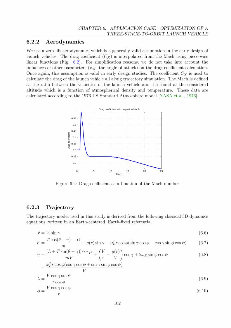
CHAPTER 6. APPLICATION CASE : OPTIMIZATION OF ATHREE-STAGE-TO-ORBIT LAUNCH VEHICLE
6.2.2 AerodynamicsWe use a zero-lift aerodynamics which is a generally valid assumption in the early design oflaunch vehicles. The drag coefficient (CX) is interpolated from the Mach using piece-wiselinear functions (Fig. 6.2). For simplification reasons, we do not take into account theinfluences of other parameters (e.g. the angle of attack) on the drag coefficient calculation.Once again, this assumption is valid in early design studies. The coefficient CX is used tocalculate the drag of the launch vehicle all along trajectory simulation. The Mach is definedas the ratio between the velocities of the launch vehicle and the sound at the consideredaltitude which is a function of atmospherical density and temperature. These data arecalculated according to the 1976 US Standard Atmosphere model [NASA et al., 1976].
0 5 10 15 20 25
0.2
0.25
0.3
0.35
0.4
0.45
0.5
0.55
Mach
Dra
g co
effic
ient
Drag coefficient with respect to Mach
Figure 6.2: Drag coefficient as a function of the Mach number
6.2.3 TrajectoryThe trajectory model used in this study is derived from the following classical 3D dynamicsequations, written in an Earth-centered, Earth-fixed referential.
r = V. sin γ
V = T cos(θ − γ)−Dm
− g(r) sin γ + ω2Er cosφ(sin γ cosφ− cos γ sinφ cosψ)
γ = [L+ T sin(θ − γ)] cosµmV
+(V
r− g(r)
V
)cos γ + 2ωE sinψ cosφ
+ ω2Er cosφ(cos γ cosφ+ sin γ sinφ cosψ)
V
λ = V cos γ sinψr cosφ
φ = V cos γ cosψr
(6.6)
(6.7)
(6.8)
(6.9)
(6.10)
102

6.2. DESCRIPTION OF THE DISCIPLINES
ψ = [L+ T sin(θ − γ)] sinµmV cos γ + V cos γ sinψ tanφ
r+ 2ωE(sinφ− cosψ cosφ tan γ)
+ ω2Er sinφ cosφ sinψ
V cos γm = −q
(6.11)
(6.12)
with :• r : radius (m),
• V : norm of the velocity vector (m.s−1),
• γ : flight path angle (rad),
• φ : latitude (rad),
• λ : longitude (rad),
• ψ : flight path heading (rad),
• µ : bank angle (rad),
• θ : pitch angle (rad),
• ωE : angular velocity of the Earth (2π/86164.09 rad/s)
• T : Thrust (N)
• D : Drag (N),
• L : Lift (N),
• g(r) : gravity acceleration at r (m2/s),
• m : mass (kg),
• q : mass flow rate (kg.s−1).The used referential is given in Figure 6.3.
Choice of state vector and model simplifications
We have chosen to use a 3 degrees of freedom non rotating round Earth model. Indeed, weonly consider a planar trajectory in the equatorial plan. We have chosen to use this modelbecause it is sufficiently representative of the real problem and it meets the main need of thisstudy which is the development of MDO methods. The introduced simplifications induce :
ψ = π
2 (6.13)
µ = 0 (6.14)φ = 0 (6.15)
103

CHAPTER 6. APPLICATION CASE : OPTIMIZATION OF ATHREE-STAGE-TO-ORBIT LAUNCH VEHICLE
RE
r
yV
DL
T
local horizon
x
Figure 6.3: Earth-centered, Earth-fixed reference frame
Consequently, we have chosen to handle the following state vector :
x=
rVγλm
with :
• α : angle of attack (rad)
• RE : Earth radius (6378.137 km)
State equations
With the simplifications described above, the state equations become :
r = V. sin γ (6.16)
V = −12ρ(r)Sref .CX(Mach)
mV 2 − g(r). sin γ + T. cos(θ − γ)
m(6.17)
γ =(V
r− g(r)
V
)cos γ + T. sin(θ − γ)
m.V(6.18)
λ = V. cos γr
(6.19)
m = −q (6.20)
with :
• Sref : aerodynamic reference surface,
104
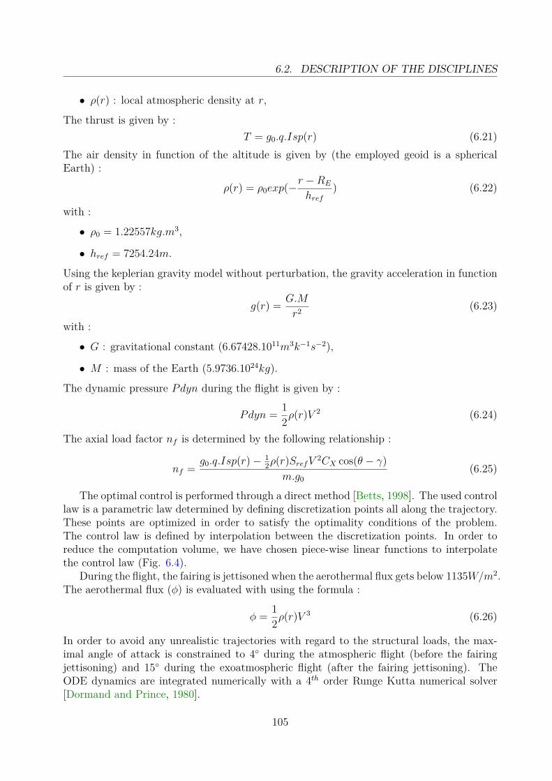
6.2. DESCRIPTION OF THE DISCIPLINES
• ρ(r) : local atmospheric density at r,
The thrust is given by :T = g0.q.Isp(r) (6.21)
The air density in function of the altitude is given by (the employed geoid is a sphericalEarth) :
ρ(r) = ρ0exp(−r −RE
href) (6.22)
with :
• ρ0 = 1.22557kg.m3,
• href = 7254.24m.
Using the keplerian gravity model without perturbation, the gravity acceleration in functionof r is given by :
g(r) = G.M
r2 (6.23)
with :
• G : gravitational constant (6.67428.1011m3k−1s−2),
• M : mass of the Earth (5.9736.1024kg).
The dynamic pressure Pdyn during the flight is given by :
Pdyn = 12ρ(r)V 2 (6.24)
The axial load factor nf is determined by the following relationship :
nf =g0.q.Isp(r)− 1
2ρ(r)SrefV 2CX cos(θ − γ)m.g0
(6.25)
The optimal control is performed through a direct method [Betts, 1998]. The used controllaw is a parametric law determined by defining discretization points all along the trajectory.These points are optimized in order to satisfy the optimality conditions of the problem.The control law is defined by interpolation between the discretization points. In order toreduce the computation volume, we have chosen piece-wise linear functions to interpolatethe control law (Fig. 6.4).
During the flight, the fairing is jettisoned when the aerothermal flux gets below 1135W/m2.The aerothermal flux (φ) is evaluated with using the formula :
φ = 12ρ(r)V 3 (6.26)
In order to avoid any unrealistic trajectories with regard to the structural loads, the max-imal angle of attack is constrained to 4◦ during the atmospheric flight (before the fairingjettisoning) and 15◦ during the exoatmospheric flight (after the fairing jettisoning). TheODE dynamics are integrated numerically with a 4th order Runge Kutta numerical solver[Dormand and Prince, 1980].
105
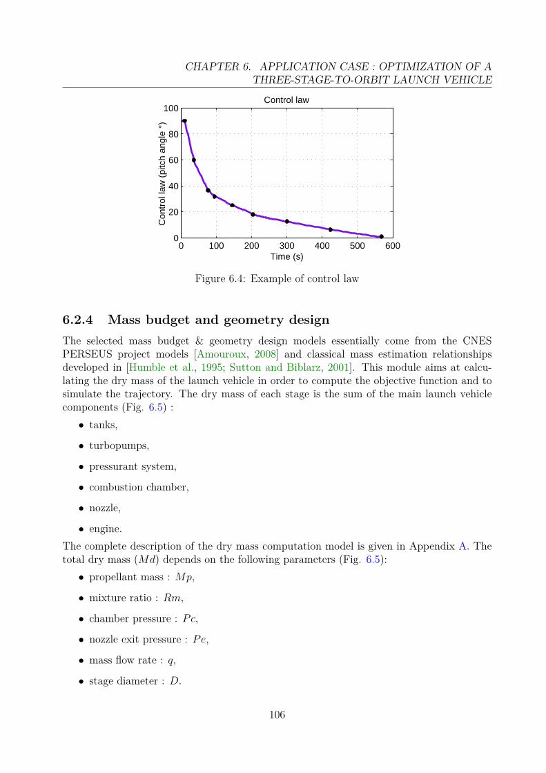
CHAPTER 6. APPLICATION CASE : OPTIMIZATION OF ATHREE-STAGE-TO-ORBIT LAUNCH VEHICLE
0 100 200 300 400 500 6000
20
40
60
80
100Control law
Time (s)
Con
trol
law
(pi
tch
angl
e °)
Figure 6.4: Example of control law
6.2.4 Mass budget and geometry designThe selected mass budget & geometry design models essentially come from the CNESPERSEUS project models [Amouroux, 2008] and classical mass estimation relationshipsdeveloped in [Humble et al., 1995; Sutton and Biblarz, 2001]. This module aims at calcu-lating the dry mass of the launch vehicle in order to compute the objective function and tosimulate the trajectory. The dry mass of each stage is the sum of the main launch vehiclecomponents (Fig. 6.5) :• tanks,
• turbopumps,
• pressurant system,
• combustion chamber,
• nozzle,
• engine.The complete description of the dry mass computation model is given in Appendix A. Thetotal dry mass (Md) depends on the following parameters (Fig. 6.5):• propellant mass : Mp,
• mixture ratio : Rm,
• chamber pressure : Pc,
• nozzle exit pressure : Pe,
• mass flow rate : q,
• stage diameter : D.
106

6.2. DESCRIPTION OF THE DISCIPLINES
Tanks sizing module
Turbopumpssizing module
Pressurant systemsizing module
Combustion chambersizing module
Nozzlesizing module
Mp
Rm
Pc
Pe
q
D
Engine sizing module
Mtank
MTP
Mpress
Mch
Mn
Madd
Md
Additional masssizing module
Meng
Figure 6.5: Dry mass sizing module
with :
• Mtank : mass of the tanks,
• Meng : mass of the engine,
• Mn : mass of the nozzle,
• Mch : mass of the combustion chamber,
• Mpress : mass of the pressurant system,
• MTP : mass of the turbopumps,
• Madd : additional masses.
In order to take into account the loads sustained by the launch vehicle during the flight, alinear dependency (cf ) of the dry mass on the maximal sustained axial load factor has beenadded into the mass sizing module (Fig. 6.6). This term introduces a coupling between thetrajectory and the mass sizing disciplines.
107

CHAPTER 6. APPLICATION CASE : OPTIMIZATION OF ATHREE-STAGE-TO-ORBIT LAUNCH VEHICLE
0 2 4 6 8 10100
105
110
115
120
c f(%)
Maximal longitudinal load factor
Evolution of load factor coefficient
Figure 6.6: Evolution of the load factor coupling coefficient with respect to the maximalaxial load factor
The total dry mass is given by the formula :
Md = [Mtanks +Meng +Mpress +MTP +Madd].cf (6.27)
The dry mass calculation module has been compared with classical cryogenic stages foundin ESA launch vehicles catalog [European Space Agency, 2004]. Results show that the mod-elization is quite valid and gives results in the same order of magnitude as the real stages(Fig. 6.7) and consequently are satisfactory for early phase design studies.
0 50 100 1500
2
4
6
8
10
12
14
Dry
mas
s(t)
Propellant mass(t)
Dry mass model
Calculated dry massReal dry mass (ESA catalog)
Ariane5EPC
Ariane5GEPC
Ariane5ESEPC
Delta4HCentaur
Ariane4H10
Athena2Centaur
H22ndstage
Atlas2,3,3B,5Centaur
Figure 6.7: Results obtained with dry mass model
108

6.3. OPTIMIZATION VARIABLES AND DISCIPLINARY INTERACTIONS
6.3 Optimization variables and disciplinary interactionsIn this section, we define the optimization variables and we describe the different interactionsbetween the considered disciplines.
6.3.1 Optimization variablesThe optimization problem for a three stage launch vehicle consists of 30 optimization vari-ables divided as follows :• 6 for the mass budget (Mpi, Rmi, i = 1, · · · , 3),
• 9 for the propulsion (Pci, Pei, T/Wi, i = 1, · · · , 3),
• 3 for the aerodynamics (Di, i = 1, · · · , 3),
• 12 for the trajectory(θij, i = 1, · · · , 3, j = 1, · · · , 4)All of the propulsion and aerodynamics variables are used in the mass budget module tocompute the dry mass. Concerning the propulsion, the selected optimization variables arethe propellant mass Mp, the mixture ratio Rm, the initial thrust to weight ratio T
W, the
chamber pressure Pc and the nozzle exit pressure Pe. We have chosen to handle the thrustto weight ratio instead of the mass flow rate q because the search domain of this parametercan be more easily estimated than the one of the mass flow rate. In order to simulate thetrajectory, a relationship between the mass flow rate and the thrust to weight ratio can beeasily determined by introducing the mass index of the considering stage. Considering theaerodynamics, the selected optimization variables are the diameters of the stages D.
6.3.2 Interactions between the different disciplinesThe following N2-Chart sums up the different interactions between the disciplines for onestage (Fig. 6.8). This chart is used to describe the data flows between the different disci-plines during the multidisciplinary analysis. This chart can be generalized to describe moregenerally the MDO methods using the same notations [Lambe, 2011].
From the diameters of the different stages, the drag coefficient is computed and trans-mitted to the trajectory module. In the same manner, the specific impulse is computed inthe propulsion module from the mixture ratio, the chamber and nozzle exit pressures. Themass budget computes the dry mass of the stages from the diameter, the mixture ratio, thechamber and nozzle pressures, the weight on thrust ratio and the propellant mass. Thismodule is in charge of the computation of the objective function (GLOW). Finally, from allthe variables, the trajectory module simulates the trajectory and returns the state vector atthe final time.
For the “mass budget” module requires the maximal load factor in order to computethe dry mass, a coupling is necessary between the trajectory and mass budget modules.This coupling induces a loop between these two disciplines and requires an estimation ofthe load factor to compute at first the dry mass and so begin the loop (Fixed Point Iter-ation). We will see later in this chapter how to handle this coupling without requiring a FPI.
109

CHAPTER 6. APPLICATION CASE : OPTIMIZATION OF ATHREE-STAGE-TO-ORBIT LAUNCH VEHICLE
AERODYNAMICS
PROPULSION
WEIGHTS/SIZING
TRAJECTORY
D Rm,Pc,Pe D,Rm,Pc,Pe,T/W,Mp u
Cd
Isp
M
nf
r,v, ,GLOWDne
Figure 6.8: N2 Chart for one stage
6.4 MDO problem formulation
6.4.1 Initial formulationUsing the mathematical MDO notations developed previously, the original formulation ofthe Launch Vehicle MDO problem is the following :
Minimize f(z) =3∑i=1
(Mpi +Mdi) +Mupper composite
With respect to z = {Mpi,TW i, Rmi, P ci, P ei, Di, θij}, i = 1, · · · , 3
Subject to g1 : |αmax 1| − 4◦ ≤ 0 (6.28)g2 : |αmax 2| − 15◦ ≤ 0 (6.29)g3...5 : 0.4− Pei
Pa(r) ≤ 0 (6.30)g6...8 : Dnei − 0.8 Di ≤ 0 (6.31)
h1 : rf − rorbit = 0 (6.32)h2 : vf − vorbit = 0 (6.33)h3 : γf − γorbit = 0 (6.34)
with θij the different variables of the control law of the ith stage (j = 1, · · · , 4).
6.4.2 MDF formulationIn order to break the FPI between the trajectory and the mass budget modules, the initialformulation has been transformed in order to perform sequentially the MDA at the subsystemlevel. To this end, an estimation of maximal load factor sustained during the flight (nfmax)has been included into the optimization variable set and a coupling constraint has beenadded to the constraint set (Eq. 6.42). We assume that the maximal load factor occursduring the flight of the first stage, that allows to introduce only one coupling variable (and
110

6.5. STAGE-WISE DECOMPOSITION FORMULATIONS
consequently one coupling constraint). This approximation is valid for expendable launchvehicles which lift off from the ground and has been verified by simulation a posteriori (oncethe optimization performed). The use of FPI is discussed in the appendix B. The resultingformulation is the following :
Minimize f(z) =3∑i=1
(Mpi +Mdi) +Mupper composite
With respect to z = {Mpi,TW i, Rmi, P ci, P ei, Di, θij}, i = 1, · · · , 3
y = {nfmax}Subject to g1 : |αmax 1| − 4◦ ≤ 0 (6.35)
g2 : |αmax 2| − 15◦ ≤ 0 (6.36)g3...5 : 0.4− Pei
Pa(r) ≤ 0 (6.37)g6...8 : Dnei − 0.8 Di ≤ 0 (6.38)
h1 : rf − rorbit = 0 (6.39)h2 : vf − vorbit = 0 (6.40)h3 : γf − γorbit = 0 (6.41)
c : nfmax −max(nfmax , nfmax) = 0 (6.42)
The use of the max in Eq. 6.42 symbolizes the fact that the configuration of the launchvehicle is still valid when the estimated maximal load factor taken into account in theweights & sizing module is greater than the real load factor observed during the trajectorysimulation. In this case, the configuration of the launch vehicle is consistent even if thestructure is oversized with respect to the sustained loads. We can note that this formulationinvolves one coupling variable (and corresponding constraint). For convenience reason, wewill use this formulation to implement the MDF method in order to save computation timeavoiding the FPI within the MDA.
6.5 Stage-wise decomposition formulations
6.5.1 First formulationIn the first formulation, all the subsystems have to minimize their own mass. Since a stageoptimizer requires the knowledge of the upper stage masses, these ones are estimated atthe system level (Mustagei) and have to be equal to the real optimized mass (Mu∗stagei) atconvergence (satisfaction of the coupling constraints (6.43) and (6.44)).
Remark 6.5.1. For all our proposed formulations, we use the angle of attack α instead ofthe pitch angle θ at the system level. The pitch angle (real control law coupling variable) isgiven by the relation θ = α+ γ. This allows to handle the inequality constraints on the angleof attack (Eq. 6.28,6.29) directly in the domain definition of the system level optimizationvariable α (bounds of the optimization variable). In the same manner, we avoid the subsystemlevel equality coupling constraints about the control law by using directly the system levelcontrol parameters (given by γ+α) as first (and last) parameters of the parametric control law
111
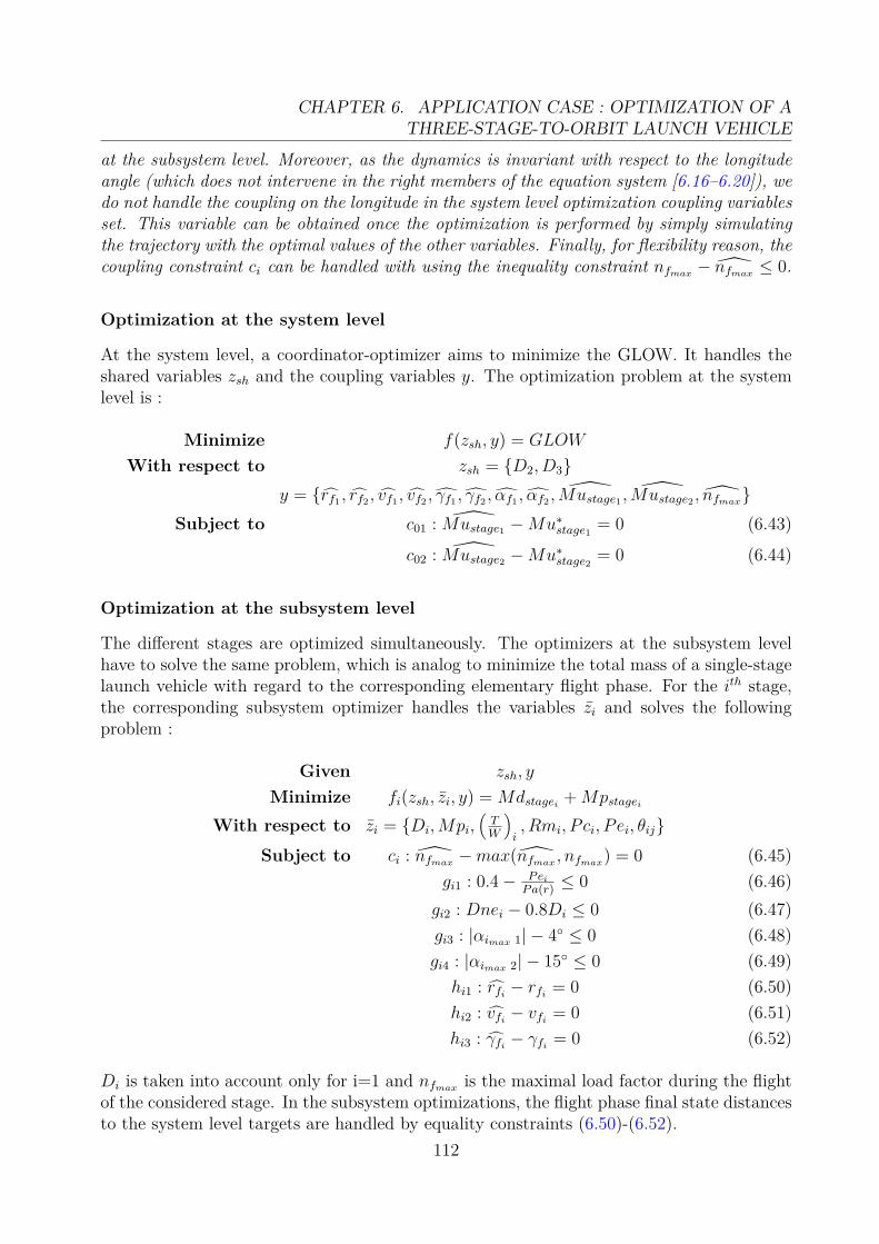
CHAPTER 6. APPLICATION CASE : OPTIMIZATION OF ATHREE-STAGE-TO-ORBIT LAUNCH VEHICLE
at the subsystem level. Moreover, as the dynamics is invariant with respect to the longitudeangle (which does not intervene in the right members of the equation system [6.16–6.20]), wedo not handle the coupling on the longitude in the system level optimization coupling variablesset. This variable can be obtained once the optimization is performed by simply simulatingthe trajectory with the optimal values of the other variables. Finally, for flexibility reason, thecoupling constraint ci can be handled with using the inequality constraint nfmax − nfmax ≤ 0.
Optimization at the system level
At the system level, a coordinator-optimizer aims to minimize the GLOW. It handles theshared variables zsh and the coupling variables y. The optimization problem at the systemlevel is :
Minimize f(zsh, y) = GLOW
With respect to zsh = {D2, D3}y = {rf1 , rf2 , vf1 , vf2 , γf1 , γf2 , αf1 , αf2 , Mustage1 , Mustage2 , nfmax}
Subject to c01 : Mustage1 −Mu∗stage1 = 0 (6.43)
c02 : Mustage2 −Mu∗stage2 = 0 (6.44)
Optimization at the subsystem level
The different stages are optimized simultaneously. The optimizers at the subsystem levelhave to solve the same problem, which is analog to minimize the total mass of a single-stagelaunch vehicle with regard to the corresponding elementary flight phase. For the ith stage,the corresponding subsystem optimizer handles the variables zi and solves the followingproblem :
Given zsh, y
Minimize fi(zsh, zi, y) = Mdstagei +Mpstagei
With respect to zi = {Di,Mpi,(TW
)i, Rmi, P ci, P ei, θij}
Subject to ci : nfmax −max(nfmax , nfmax) = 0 (6.45)gi1 : 0.4− Pei
Pa(r) ≤ 0 (6.46)gi2 : Dnei − 0.8Di ≤ 0 (6.47)gi3 : |αimax 1| − 4◦ ≤ 0 (6.48)gi4 : |αimax 2| − 15◦ ≤ 0 (6.49)hi1 : rfi − rfi = 0 (6.50)hi2 : vfi − vfi = 0 (6.51)hi3 : γfi − γfi = 0 (6.52)
Di is taken into account only for i=1 and nfmax is the maximal load factor during the flightof the considered stage. In the subsystem optimizations, the flight phase final state distancesto the system level targets are handled by equality constraints (6.50)-(6.52).
112

6.5. STAGE-WISE DECOMPOSITION FORMULATIONS
6.5.2 Second formulationThis formulation uses the classical Collaborative Optimization [Braun et al., 1996] appliedto the stage-wise decomposition.
Optimization at the system level
In this formulation, the system level optimizer does not control explicitly the couplingsabout the different stage payload masses anymore but only ensures that at the convergence,the objective functions of the subsystems are equal to zero. Thus, three equality constraints(Eq.(6.53)-(6.55)) have to be handled at the system level and an additional variable (GLOW ,estimation of the GLOW) is added to the problem.
Minimize f(zsh, y) = GLOW
With respect tozsh = {D2, D3}
y = {rf1 , rf2 , vf1 , vf2 , γf1 , γf2 , αf1 , αf2 , GLOW, Mustage1 , Mustage2 , nfmax}
Subject toc01 : f ∗1 = 0 (6.53)c02 : f ∗2 = 0 (6.54)c03 : f ∗3 = 0 (6.55)
Optimization at the subsystem level
At the subsystem level, all the equality constraints h do not appear explicitly and are includedin the objective function. Indeed, each stage aims at minimizing a quadratic sum betweenreal values and targets given by the system level optimizer. In this formulation, the couplingsabout the different stage masses are also taken into account in the objective function.
Given zsh, y
Minimizefi(zsh, zi, y) =
(rfi − rfi
R
)2
+(vfi − vfi
V
)2
+(γfi − γfi
Γ
)2
+Mpi +Mdi + Mustagei − Mustagei−1
M
2
With respect to zi = {Di,Mpi,(T
W
)i, Rmi, P ci, P ei, θij}
Subject to
ci : nfmax −max(nfmax , nfmax) = 0 (6.56)
gi1 : 0.4− PeiPa(r) ≤ 0 (6.57)
gi2 : Dnei − 0.8Di ≤ 0 (6.58)gi3 : |αimax 1| − 4◦ ≤ 0 (6.59)gi4 : |αimax 2| − 15◦ ≤ 0 (6.60)
with R, V , Γ and M different normalization weights on the objective function,Mustage0 = GLOW and Di is only considered for i=1 in Eq. (6.5.2).
113

CHAPTER 6. APPLICATION CASE : OPTIMIZATION OF ATHREE-STAGE-TO-ORBIT LAUNCH VEHICLE
6.5.3 Third formulation
The third formulation removes all the equality constraints at the system level. Moreover,the estimated mass of the different stages are also removed from the optimization problem.In this formulation, the optimizations of the different subsystems are performed sequentiallyfrom the uppermost stage to the lowermost one. The stage masses are transmitted betweenthe different subsystems without any action of the system level optimizer, that allows toautomatically satisfy the mass couplings between the stages. In that way, all the couplingconstraints concerning the state vector are satisfied at the subsystem level.
Optimization at the system level
At the system level, the coupling variables about the masses are removed.
Minimize f(zsh, y) = GLOW
With respect to zsh = {D2, D3}y = {rf1 , rf2 , vf1 , vf2 , γf1 , γf2 , αf1 , αf2 , nfmax}
Optimization at the subsystem level
At the subsystem level, the optimizations of the different stages can not be performed inde-pendently anymore. The flight phase final state distances to the desired values are handledas equality constraints. The subsystem level optimization problems are the same as in thefirst formulation.i=3While i > 0
Given zsh, y, f∗k,k>i
Minimize fi(zsh, zi, y) = Mdstagei +Mpstagei
With respect to zi = {Di,Mpi,(TW
)i, Rmi, P ci, P ei, θij}
Subject to ci : nfmax −max(nfmax , nfmax) = 0 (6.61)gi1 : 0.4− Pei
Pa(r) ≤ 0 (6.62)gi2 : Dnei − 0.8.Di ≤ 0 (6.63)gi3 : |αimax 1| − 4◦ ≤ 0 (6.64)gi4 : |αimax 2| − 15◦ ≤ 0 (6.65)hi1 : rfi − rfi = 0 (6.66)hi2 : vfi − vfi = 0 (6.67)hi3 : γfi − γfi = 0 (6.68)
i=i-1where Di is taken into account only for i=1.
114
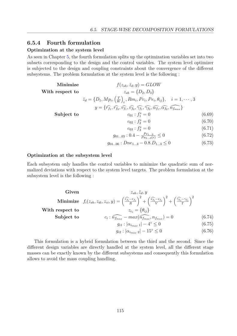
6.5. STAGE-WISE DECOMPOSITION FORMULATIONS
6.5.4 Fourth formulationOptimization at the system levelAs seen in Chapter 5, the fourth formulation splits up the optimization variables set into twosubsets corresponding to the design and the control variables. The system level optimizeris subjected to the design and coupling constraints about the convergence of the differentsubsystems. The problem formulation at the system level is the following :
Minimize f(zsh, zd, y) = GLOW
With respect to zsh = {D2, D3}zd = {D1,Mpi,
(TW
)i, Rmi, P ci, P ei, θij}, i = 1, · · · , 3
y = {rf1 , rf2 , vf1 , vf2 , γf1 , γf2 , αf1 , αf2 , nfmax}Subject to c01 : f ∗1 = 0 (6.69)
c02 : f ∗2 = 0 (6.70)c03 : f ∗3 = 0 (6.71)
g01...03 : 0.4− Pe1...3Pa1...3(r) ≤ 0 (6.72)
g04...06 : Dne1...3 − 0.8.D1...3 ≤ 0 (6.73)
Optimization at the subsystem level
Each subsystem only handles the control variables to minimize the quadratic sum of nor-malized deviations with respect to the system level targets. The problem formulation at thesubsystem level is the following :
Given zsh, zd, y
Minimize fi(zsh, zdi, zci, y) =(rfi−rfi
R
)2+(vfi−vfi
V
)2+(γfi−γfi
Γ
)2
With respect to zci = {θij}Subject to ci : nfmax −max(nfmax , nfmax) = 0 (6.74)
gi1 : |αimax 1| − 4◦ ≤ 0 (6.75)gi2 : |αimax 2| − 15◦ ≤ 0 (6.76)
This formulation is a hybrid formulation between the third and the second. Since thedifferent design variables are directly handled at the system level, all the different stagemasses can be exactly known by the different subsystems and consequently this formulationallows to avoid the mass coupling handling.
115

CHAPTER 6. APPLICATION CASE : OPTIMIZATION OF ATHREE-STAGE-TO-ORBIT LAUNCH VEHICLE
6.6 ConclusionIn this chapter, we have detailed the three-stage-to-orbit LVD problem. To this end, wehave briefly described the different variables, the different disciplines and the interactionsbetween them. Secondly, the initial MDO formulation of the problem has been detailed. Acoupling variable (and corresponding constraint) have been introduced in order to performsequentially the multidisciplinary analysis. The proposed MDO formulations have beenexplained within the framework of the three-stage-launch-vehicle application case.
The study case described in this chapter will be used in the next chapter to numericallycompare the proposed MDO formulations.
116

Chapter 7
Comparison of the differentformulations
Contents7.1 Introduction . . . . . . . . . . . . . . . . . . . . . . . . . . . . . . 1177.2 Analysis of the problem dimensionality and the number of con-
straints . . . . . . . . . . . . . . . . . . . . . . . . . . . . . . . . . . 1187.3 Qualitative comparison of proposed formulations . . . . . . . . 1207.4 Numerical comparison of the formulations . . . . . . . . . . . . 122
7.4.1 Context . . . . . . . . . . . . . . . . . . . . . . . . . . . . . . . . . 1227.4.2 Adaptation of stage-wise formulations to genetic algorithm . . . . 1247.4.3 Results and analysis . . . . . . . . . . . . . . . . . . . . . . . . . . 1257.4.4 Limitations of the numerical comparison . . . . . . . . . . . . . . . 132
7.5 Conclusion . . . . . . . . . . . . . . . . . . . . . . . . . . . . . . . 132
7.1 Introduction
This chapter is devoted to the comparison of the different proposed formulations [Balesdentet al., 2010a, 2011c]. In order to perform this comparison, we have to select a referencemethod which will be used as reference point to evaluate the efficiency of the differentformulations. In order to be representative of the papers relative to LVD in literature,we have chosen to compare the different formulations with respect to the MDF method.Indeed, as detailed in Chapter 4, the most used MDO method in LVD appears to be theMDF method. In fact, in Table 4.1, about three quarters of the surveyed papers involve aMDF method to solve the LVD problem.In the first section of this chapter, we compare analytically the characteristics of the differentformulations with respect to the MDF method. Then, we compare numerically the differentformulations using the same optimization algorithms.
117

CHAPTER 7. COMPARISON OF THE DIFFERENT FORMULATIONS
7.2 Analysis of the problem dimensionality and thenumber of constraints
The different proposed formulations do not handle the same numbers of optimization vari-ables and constraints at the system level. This characteristic has directly an impact on thedimension of the search space and the choice of the optimization algorithms to use. In thissection, we study analytically the dimension of the search spaces and the number of con-straints with respect to some characteristics of the launch vehicle design problem in orderto compare theoretically the different formulations and to expose their advantages and thedrawbacks. The numbers in parentheses are the current values taken by the variables forthe considered study case (cf Chapter 6).Let us consider :
• ne : number of stages (3),
• nx : dimension of the state vector (5 : altitude, velocity, flight path angle, longitudeand mass),
• nc : dimension of the control law variables vector (1 : pitch angle),
• npp : number of control law discretization points per stage (4),
• npsh : number of design variables per stage which play a part in the flight phases ofseveral stages (1 : diameter of the stage),
• npk : number of design variables per stage which only play a part in the kth stage flightphase (5 : mixture ratio, chamber pressure, nozzle exit pressure, propellant mass andinitial thrust to weight ratio).
The search space dimensions are given by the following relationships:
nMDF = ne.(npk + nc.npp + npsh) + 1 (7.1)nfirst formulation = (ne − 1).(nx − 2) + (ne − 1).nc + (ne − 1).npsh + 1 + (ne − 1)(7.2)nsecond formulation = (ne − 1).(nx − 2) + (ne − 1).nc + (ne − 1).npsh + 1 + ne (7.3)nthird formulation = (ne − 1).(nx − 2) + (ne − 1).nc + (ne − 1).npsh + 1 + 0 (7.4)nfourth formulation = (ne − 1).(nx − 2) + (ne − 1).nc + ne.npsh + ne.npk + 1 (7.5)
In the same manner, the numbers of constraints at the system level are given by :
ncMDF= 3.ne + (nx − 2) + 2 (7.6)
ncfirst formulation = (ne − 1) (7.7)ncsecond formulation = ne (7.8)ncthird formulation = 0 (7.9)nfourth formulation
= ne + 2.ne (7.10)
By decomposing the optimization problem, the search domains of each optimizationprocess at the system and subsystem levels are considerably reduced in comparison with
118

7.2. ANALYSIS OF THE PROBLEM DIMENSIONALITY AND THE NUMBER OFCONSTRAINTS
MDF which involves a single optimizer to handle all the optimization variables. Indeed,in the MDF method, the dimension of the optimizer search domain concerning the currentapplication case is 31, while the system level optimizers of the first, second, third and fourthstage-wise decomposition formulations have to handle respectively 13, 14, 11 and 27 vari-ables. In the same manner, the MDF optimizer problem is very constrained (8 inequalityand 6 equality constraints). The stage-wise decomposition formulations allow the distribu-tion of the constraints on the system and the subsystem levels. Table 7.1 summarizes thenumber of constraints and variables handled by the MDF and the stage-wise decompositionformulation system level optimizers. The values in green (respectively in red) represent thebest (respectively the worst) values.
MDF F1 F2 F3 F4Number of variables for the three-stage configuration 31 13 14 11 27Number of additional variables when adding a stage 10 6 6 5 9Number of constraints for the three-stage configuration 14 4 5 0 9Number of additional constraints when adding a stage 3 1 1 0 3
Table 7.1: Synthesis of the optimization problems complexity at the system level
The evolutions of the search domain dimensions and the numbers of constraints withrespect to the number of stages are given in Figure 7.1. This figure points that the morestages the optimization problem involves, the better are the stage-wise decomposition for-mulations with respect to the MDF method. Globally, the third formulation is the onewhich presents the best characteristics. Indeed, this method does not require any constraintat the system level, involves the lowest number of coupling variables (i.e. the lowest searchdomain dimension) and ensures the coupling consistency between the different subsystemsat each iteration. This characteristic allows the user to have consistent solutions even if thealgorithm at the system level has not converged yet, which is not the case with using thefirst, second and fourth formulations.
2 3 40
10
20
30
40
50Dimension of search space
Dim
ensi
on o
f sea
rch
spac
e
Number of stages
MDF F1 F2 F3 F4
2 3 40
5
10
15
20Number of constraints
Num
ber
of c
onst
rain
ts
Number of stages
Figure 7.1: Search domain and number of constraints at the system level w.r.t. the numberof stages
119
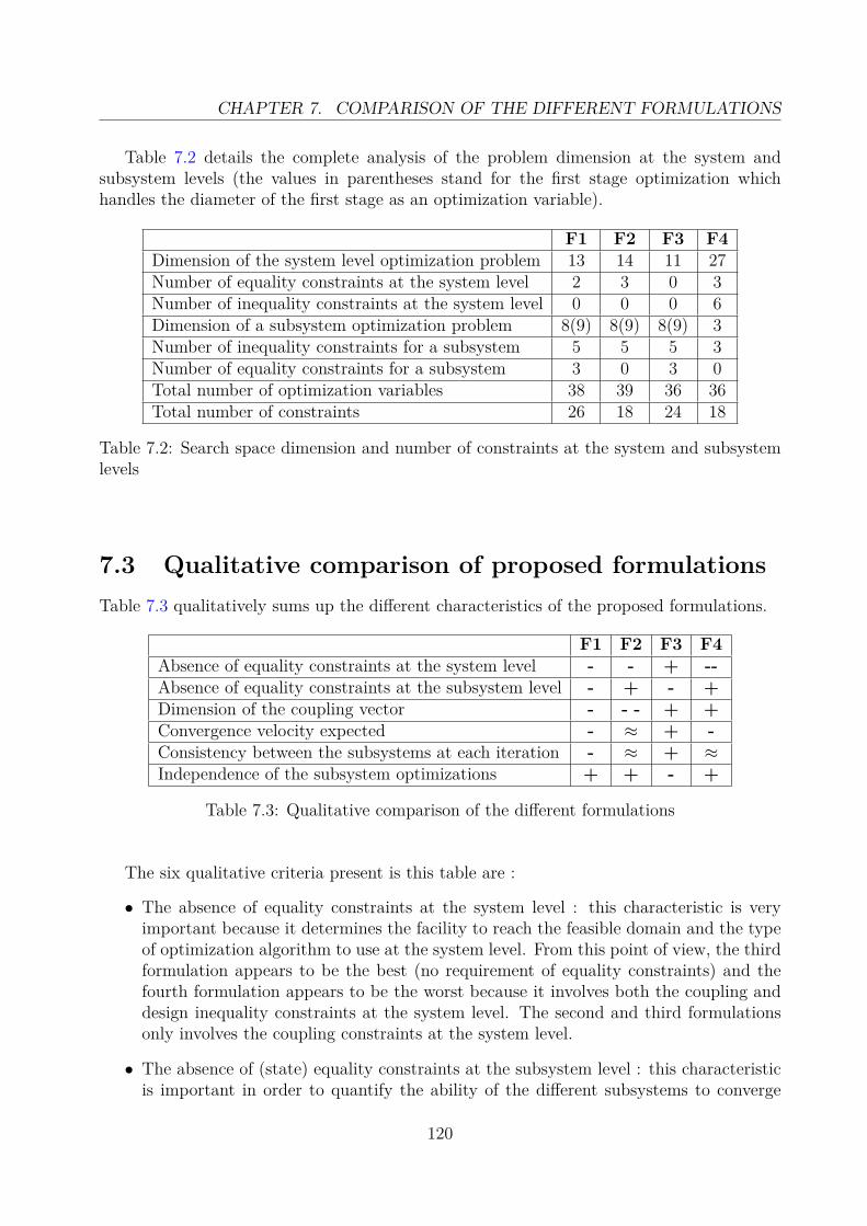
CHAPTER 7. COMPARISON OF THE DIFFERENT FORMULATIONS
Table 7.2 details the complete analysis of the problem dimension at the system andsubsystem levels (the values in parentheses stand for the first stage optimization whichhandles the diameter of the first stage as an optimization variable).
F1 F2 F3 F4Dimension of the system level optimization problem 13 14 11 27Number of equality constraints at the system level 2 3 0 3Number of inequality constraints at the system level 0 0 0 6Dimension of a subsystem optimization problem 8(9) 8(9) 8(9) 3Number of inequality constraints for a subsystem 5 5 5 3Number of equality constraints for a subsystem 3 0 3 0Total number of optimization variables 38 39 36 36Total number of constraints 26 18 24 18
Table 7.2: Search space dimension and number of constraints at the system and subsystemlevels
7.3 Qualitative comparison of proposed formulationsTable 7.3 qualitatively sums up the different characteristics of the proposed formulations.
F1 F2 F3 F4Absence of equality constraints at the system level - - + --Absence of equality constraints at the subsystem level - + - +Dimension of the coupling vector - - - + +Convergence velocity expected - ≈ + -Consistency between the subsystems at each iteration - ≈ + ≈Independence of the subsystem optimizations + + - +
Table 7.3: Qualitative comparison of the different formulations
The six qualitative criteria present is this table are :
• The absence of equality constraints at the system level : this characteristic is veryimportant because it determines the facility to reach the feasible domain and the typeof optimization algorithm to use at the system level. From this point of view, the thirdformulation appears to be the best (no requirement of equality constraints) and thefourth formulation appears to be the worst because it involves both the coupling anddesign inequality constraints at the system level. The second and third formulationsonly involves the coupling constraints at the system level.
• The absence of (state) equality constraints at the subsystem level : this characteristicis important in order to quantify the ability of the different subsystems to converge
120

7.3. QUALITATIVE COMPARISON OF PROPOSED FORMULATIONS
from any instructions prescribed by the system level. In this matter, the first and thirdformulations present the worst characteristics because they involve the equality cou-pling constraints dealing with the reach of the final flight phase state at the subsystemlevel. The formulations 2 and 4 allow to avoid these equality constraints, consideringthe reach of the final state directly in the subsystem objective functions.
• The dimension of the coupling vector : the third and fourth formulations present thelowest dimension of the coupling vector because they do not require the estimations ofthe stage payload masses. The second formulation presents the largest coupling vectorbecause it includes the estimation of the GLOW in addition to the estimated payloadmasses.
• The expected convergence velocity : this characteristic is fundamental and dependspartially on the search space dimension and equality constraints at the system level.From this point of view, the third formulation expects to have the best convergencevelocity because the system level does not have any equality constraint and showsthe lowest optimization variable set to handle. Contrariwise, the fourth formulationmay pose problems because the system level has to handle the design variables (andcorresponding constraints) in addition to the shared and coupling variables.
• The consistency between the subsystems at each iteration : from this point of view,only the third formulation ensures the consistency between the subsystems at eachiteration of the system level optimization. Indeed, in this formulation, the only con-ditions to have a feasible design is the convergence of the different subsystems. Forthe formulations 2 and 4, due to the fact that the subsystem level objective functionminimization and the satisfaction of the system level (coupling) equality go the sameway, we may expect to reach the feasible domain rather quickly in the optimizationprocess. Contrariwise, concerning the first formulation, the feasibility of the designdepends not only on the subsystem convergence (satisfaction of equality constraints)but also the system level coupling equality constraint satisfaction. Furthermore, inthis formulation, the minimization of the subsystem objective functions and the satis-faction of the system level coupling constraints do not go the same way. Consequently,we may expect a rather low convergence velocity of this formulation.
• The independence of the different subsystem optimizations : in this matter, only thethird formulation does not allow the parallel optimizations of the different subsys-tems. Indeed, due to the mass couplings which are handled directly at the subsystemlevel, this method involves a nonhierarchical decomposition and the optimization ofthe different stages cannot be performed in parallel.
Globally, the third formulation is the formulation which presents the best qualitativecharacteristics. The only drawbacks of this formulation are the requirement of the equalityconstraints at the subsystem level and the impossibility to perform in parallel the differentsubsystem optimizations.
121

CHAPTER 7. COMPARISON OF THE DIFFERENT FORMULATIONS
7.4 Numerical comparison of the formulations
7.4.1 ContextIn order to complete the previous theoretical analysis, a numerical comparison of the differ-ent formulations has to be performed. In order to be relatively independent of the tuningsof the optimizers, we have chosen to perform this comparison in global search study. Indeed,the objective of this comparison is to quantify the ability of the different formulations tofind feasible designs and to optimize them in the case of large search space, standard tuningson the optimization algorithms and without any a priori knowledge on the feasible solutiondomain. In that way, we have chosen to perform the comparison using a Genetic Algorithmat the system level. This algorithm is the most used evolutionary algorithm in LVD. Manyexamples of application of GA in case of LVD studies can be found in literature [Schoonoveret al., 2000; Duranté et al., 2004, 2005; Akhtar and Linshu, 2005a; Bairstow et al., 2006; Bay-ley et al., 2008; Castellini et al., 2008], etc. A recent study [Rafique et al., 2010] shows thebenefits of the use of GA with respect to other heuristics such as Particle Swarm Optimiza-tion (PSO) and Simulated Annealing (SA) in air launched vehicle in terms of quality of theoptimum, even if the PSO presents better characteristics in terms of computation time. Theproblem considered in this study present analog characteristics (three-stage configuration,same objective function, disciplines, modelization of the trajectory, constraints, optimizationvariables) as the problem we want to solve, even if the launch vehicle considered in [Rafiqueet al., 2010] does not lift off from the ground. However, the problem solved in this studyconsiders very low space search (in terms of bounds on the optimization variables), which isnot the case in our study. A global comparative study of the most common heuristics in caseof launch vehicle design can be found in [Castellini and Lavagna, 2009]. This study showsthe superiority of the GA in case of non linear constraints and non convex (multi)objectivefunction.
The comparative study is not only focused on the value of the best found design but alsoon the way to reach it. Indeed, the aim of this study is not to find the best tunings of the GAin order to the reach the best performances of the optimization process but to compare theeffects of the problem formulation on the optimization process, and to verify that the thirdproposed formulation is more appropriate to solve the LVD problem. For this comparison,we suppose that :
• the user does not know an appropriate initialization of the optimization process,
• the user does not have a priori knowledge on the search domain (bounds of the opti-mization variables are very large),
• the user has not an accurate idea of the fine tunings on the GA parameters.
Consequently, we have chosen to perform the optimization in case of random initializationand using standard tunings on the GA. The bounds of the optimization variables have beenchosen very large in order to reflect the non a priori knowledge of the user concerning thesearch domain (Table 7.4). The results obtained with using the MDF method and a standardgradient-based algorithm in case of large search space are discussed in Appendix B.
122

7.4. NUMERICAL COMPARISON OF THE FORMULATIONS
Variables Lower bounds Upper bounds
Propellant mass (t)Mp1 60 100Mp2 10 40Mp3 5 25
Mixture ratioRm1 3 6Rm2 3 6Rm3 3 6
Thrust to weight ratioT/W1 1 3T/W2 0.5 2.5T/W3 0.1 2
Chamber pressure (bar)Pc1 80 120Pc2 40 80Pc3 20 60
Nozzle exit pressure (bar)Pe1 0.01 1Pe2 0.001 1Pe3 0.0001 1
Diameter (m)D1 3 5D2 3 5D3 3 5
Maximal load factor nfmax 4 6
Control law 1st stage (◦)
θ11 40 60θ12 25 45θ13 20 40θ14 15 35
Control law 2nd stage (◦)
θ21 10 30θ22 5 25θ23 5 25θ24 0 20
Control law 3rd stage (◦)
θ31 -10 10θ32 -15 5θ33 -20 0θ34 -25 -5
Altitude at stage separations (km) rf1 30 130rf2 150 250
Velocity at stage separations (km/s) vf1 1 5vf2 4 8
Flight path angle at stage separations (◦) γf1 0 50γf2 -10 40
Pitch angle at stage separations (◦) αf1 -4 4αf2 -15 15
Estimated mass (t)GLOW 130 170Mu1 40 60Mu2 10 25
Table 7.4: Bounds of the optimization variables
123
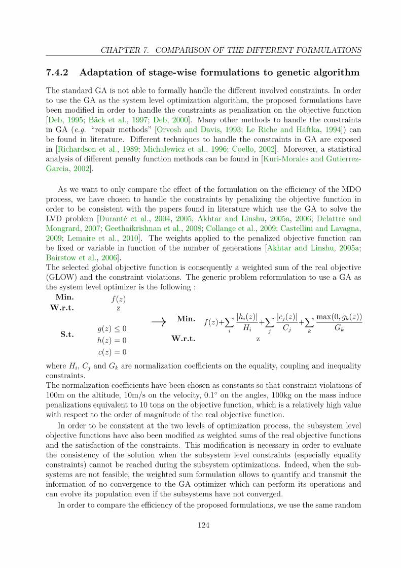
CHAPTER 7. COMPARISON OF THE DIFFERENT FORMULATIONS
7.4.2 Adaptation of stage-wise formulations to genetic algorithm
The standard GA is not able to formally handle the different involved constraints. In orderto use the GA as the system level optimization algorithm, the proposed formulations havebeen modified in order to handle the constraints as penalization on the objective function[Deb, 1995; Bäck et al., 1997; Deb, 2000]. Many other methods to handle the constraintsin GA (e.g. “repair methods” [Orvosh and Davis, 1993; Le Riche and Haftka, 1994]) canbe found in literature. Different techniques to handle the constraints in GA are exposedin [Richardson et al., 1989; Michalewicz et al., 1996; Coello, 2002]. Moreover, a statisticalanalysis of different penalty function methods can be found in [Kuri-Morales and Gutierrez-Garcia, 2002].
As we want to only compare the effect of the formulation on the efficiency of the MDOprocess, we have chosen to handle the constraints by penalizing the objective function inorder to be consistent with the papers found in literature which use the GA to solve theLVD problem [Duranté et al., 2004, 2005; Akhtar and Linshu, 2005a, 2006; Delattre andMongrard, 2007; Geethaikrishnan et al., 2008; Collange et al., 2009; Castellini and Lavagna,2009; Lemaire et al., 2010]. The weights applied to the penalized objective function canbe fixed or variable in function of the number of generations [Akhtar and Linshu, 2005a;Bairstow et al., 2006].The selected global objective function is consequently a weighted sum of the real objective(GLOW) and the constraint violations. The generic problem reformulation to use a GA asthe system level optimizer is the following :
Min. f(z)W.r.t. z
S.t.g(z) ≤ 0h(z) = 0c(z) = 0
→ Min. f(z)+∑i
|hi(z)|Hi
+∑j
|cj(z)|Cj
+∑k
max(0, gk(z))Gk
W.r.t. z
where Hi, Cj and Gk are normalization coefficients on the equality, coupling and inequalityconstraints.The normalization coefficients have been chosen as constants so that constraint violations of100m on the altitude, 10m/s on the velocity, 0.1◦ on the angles, 100kg on the mass inducepenalizations equivalent to 10 tons on the objective function, which is a relatively high valuewith respect to the order of magnitude of the real objective function.
In order to be consistent at the two levels of optimization process, the subsystem levelobjective functions have also been modified as weighted sums of the real objective functionsand the satisfaction of the constraints. This modification is necessary in order to evaluatethe consistency of the solution when the subsystem level constraints (especially equalityconstraints) cannot be reached during the subsystem optimizations. Indeed, when the sub-systems are not feasible, the weighted sum formulation allows to quantify and transmit theinformation of no convergence to the GA optimizer which can perform its operations andcan evolve its population even if the subsystems have not converged.
In order to compare the efficiency of the proposed formulations, we use the same random
124

7.4. NUMERICAL COMPARISON OF THE FORMULATIONS
initializations, the same optimization algorithm and the same tunings at the system and thesubsystem levels. Depending on the different used methods, the objective function can varyaccording to the number of constraints present in the optimization problem. The controlparameters used for the Genetic Algorithm are the followings :
Population size 100Probability of mutation 0.1Probability of crossover 0.5Probability of selection 0.05Elitism enabledStop criterion 10 hours
Table 7.5: Used GA parameters for the comparison7.4.3 Results and analysisIn order to compare the different formulations with respect to the MDF method at a fixedcalculation time, we take into account the three following criteria :
• the value of the objective function at the optimization process stop,
• the elapsed time to find a first feasible design from a random initialization,
• the improvement of the objective function between the first and the best feasible de-signs.
Due to the stochastic nature of GA, this study has been perform with 10 random initial-izations. The chosen stop criterion is calculation time (10 hours). Consequently, the nec-essary calculation time for the whole comparison is 500hours. Concerning the optimizationalgorithm, we use the MOGA-II algorithm [Poles, 2003] of the modeFRONTIER platformas the system level optimizer and a SQP algorithm implemented in the fmincon MATLABfunction as the subsystem level optimizer. Figure 7.2 shows the results obtained for thedifferent formulations. Figure 7.3 details the result for one case (8th initialization). Theresults are given in function of the elapsed time and the number of generations.
Quality of the best found design in a given time
One of the most representative characteristics to compare the different formulations is natu-rally the average best obtained design at the stopping time of the optimization process. Forsimplicity reasons, we note f ∗MDF (respectively f ∗F1, f ∗F2, f ∗F3, f ∗F4) the best design found bythe MDF (respectively the first, second, third and fourth) formulations, f ∗ the mean valueof f ∗ and σf∗ the corresponding standard deviation.
As expected according to the theoretical analysis, the third formulation is the one whichpresents the best characteristics in terms of quality of the objective function. Indeed, thisformulation induces both the best average value of the optimized GLOW (143.2t) and theminimal standard deviation (1.84t). The third formulation finds the best designs in eightinitializations out of ten.
125

CHAPTER 7. COMPARISON OF THE DIFFERENT FORMULATIONS
MDF F1 F2 F3 F4140
145
150
155
160
Ave
rage
GLO
W (
t)
Average best designs found
MDF F1 F2 F3 F40
2
4
6
σ GLO
W (
t)
Standard deviation of best designs found
MDF F1 F2 F3 F40
100
200
300
400
500
Ave
rage
ela
psed
tim
e (m
in)
Average elapsed time to find a feasible design
MDF F1 F2 F3 F40
20
40
60
80
100
σ Ela
psed
tim
e (m
in)
Standard deviation of elapsed time to find a feasible design
MDF F1 F2 F3 F4140
145
150
155
160
Ave
rage
firs
t 1st
des
ign
(t)
Average 1st feasible design
MDF F1 F2 F3 F40
2
4
6
σ 1st d
esig
n (t)
Standard deviation of 1st feasible design
MDF F1 F2 F3 F4−15
−10
−5
0
Ave
rage
impr
ovem
ent (
%)
Average improvement of the objective function
MDF F1 F2 F3 F40
1
2
3
4
σ Impr
ovem
ent (
%)
Standard deviation of the objective function
MDF F1 F2 F3 F4140
145
150
155
160
165
GLO
W (
t)
Boxplot of the best found design
MDF F1 F2 F3 F40
100
200
300
400
Ela
psed
tim
e (m
in)
Boxplot of the elapsed time
MDF F1 F2 F3 F4145
150
155
160
165
170
1st fe
asib
le d
esig
n (t
)
Boxplot of the 1st feasible design
MDF F1 F2 F3 F4−15
−10
−5
0
Impr
ovem
ent (
%)
Boxplot of the improvement
Figure 7.2: Statistical results of the comparison
The second formulation finds the best designs in the two other cases. The average valueof the optimized GLOW for the second formulation is equal to 147t and its correspondingstandard deviation is equal to 3.3t. The three other formulations lead to average bestdesigns above 150t (156t for MDF, 152t for F1 and 157.3t for F4). Globally, the first threeformulations allow to obtain better results than the MDF method, both in terms of averagevalue and standard deviation of the objective function (Eq. 7.11,7.12).
f ∗F3 < f ∗F2 < f ∗F1 < f ∗MDF < f ∗F4 (7.11)σf∗
F3< σf∗
F1< σf∗
F2< σf∗
F4< σf∗
MDF(7.12)
where f stands for the average value of f and σf its corresponding standard deviation.
The performances of the third formulation can be explained by the fact that this formu-lation induces the lowest dimension of the search domain at the system level and the absenceof coupling constraints at this level, that simplifies the optimizer task. Even if the secondformulation involves a greater search domain dimension at the system level than the first
126

7.4. NUMERICAL COMPARISON OF THE FORMULATIONS
formulation, the CO formulation used in F2 allows to satisfy more easily the coupling con-straints, that allows the optimizer to perform more easily the optimization of the objectivefunction than F1 for which the optimizer has to satisfy the coupling constraints about theequivalent payload masses of the different stages. The relatively bad results obtained for theMDF and the fourth formulations can be explained by the important number of optimizationvariables and constraints at the system level that makes global search very difficult and leadto relatively inconsistent results (the dispersions of the designs are the greatest with theMDF and the fourth formulations). This point will be detailed in the paragraph concerningthe improvement of the objective function.
0 2 4 6 8 10140
145
150
155
160
165
GLO
W(t
)
Time (h)
Evolution of GLOW (feasible designs)
0 2 4 6 8 10
10−2
100
102
104
106
108
Pen
aliz
atio
n co
effic
ient
Time(h)
Evolution of the penalization coefficient
0 2 4 6 8 1010
5
106
107
108
Pen
aliz
ed o
bjec
tive
func
tion
Time(h)
Evolution of the penalized objective
MDFF1F2F3F4
Feasible domain
Non feasible domain
(a) Penalization coefficient, penalized and real objective functions w.r.t. elapsed time
100
101
102
103
140
145
150
155
160
165
GLO
W(t
)
Number of generations
Evolution of GLOW (feasible designs)
100
101
102
103
10−2
100
102
104
106
108
Pen
aliz
atio
n co
effic
ient
Number of generations
Evolution of the penalization coefficient
100
101
102
103
105
106
107
108
Pen
aliz
ed o
bjec
tive
func
tion
Number of generations
Evolution of the penalized objective
MDFF1F2F3F4Non feasible domain
Feasible domain
(b) Penalization coefficient, penalized and real objective functions w.r.t. number of generations
Figure 7.3: Results obtained for the 8th random initialization
Calculation time required to find a first feasible design
For simplicity reasons we note t0MDF(respectively t0F1 , t0F2 , t0F3 and t0F4) the required com-
putation time to find a first feasible design for the MDF (respectively first, second, third andfourth) formulations. Figure 7.2 shows that the third formulation clearly outperforms theothers again in terms of elapsed time to find a feasible design. Indeed, the average elapsed
127

CHAPTER 7. COMPARISON OF THE DIFFERENT FORMULATIONS
time for the third formulation is only 30min while the MDF, second, fourth and first formu-lations require respectively 2h, 2h15, 3h35 and 6h45. Moreover, the third formulation showsthe lowest standard deviation, that indicates a relative stability of the results.This ranking of the formulations can be partly explained by the number of constraints andthe handling of the coupling variables at the system level. Indeed, in the third formulation,the system level optimizer has only to coordinate the different stages with respect to theposition and velocity at the stage separations (no mass coupling), all the complexity of theoptimization is transferred to the different subsystems. In this matter, the feasibility ofthe found design is only subject to the convergence of the different subsystems (i.e. thepenalization terms of the subsystem objective functions are below the fixed tolerances). Thestandard deviation of t0F3 is low comparatively to the other formulations. Indeed, this for-mulation allows to find a feasible design directly in the initialization in 8 cases out of ten(first generation), that explains both the average value and the standard deviation of t0F3 .
The average calculation times to find a first feasible design of the MDF and the secondformulation are very close. Concerning the MDF method, this result can be explained by thefact that the MDF method does not involve any optimization at the subsystem level. Indeed,for the MDF formulation, the necessary subsystem level analysis time to compute the objec-tive function and the different constraints is very short (about 1 second) comparatively to astage optimization (which takes between 20sec and 1min). Therefore, the GA can performmany more generations in order to decrease the penalized objective function and so to satisfythe constraints, even if these constraints are numerous and quite difficult to satisfy. Table7.6 resumes the average number of generations required to find a feasible design. In 2h, theGA used for the MDF formulation is able to perform 230 generations whereas for the secondformulation, the GA is only able to perform 4.6 generations in 2h15. This phenomenon canexplain the quite good results obtained for the MDF formulation. Nevertheless, the standarddeviation of this indicator is very important for this formulation, due to the fact that thetime to find a feasible design is highly dependent on the initialization.
Concerning the second formulation, the average value of t0F2 can be explained by the factthat in this formulation, the convergence of the different subsystems and the satisfaction ofthe equality constraints of the system level go the same way. Therefore, even if GA onlyperforms 4.6 generations during two hours, this formulation of the MDO problem allows tofind a feasible design in far fewer generations than MDF. The standard deviation of t0F2 isbetter than the MDF formulation but is still relatively important.
The first formulation shows the worst results in terms of elapsed time to find a feasibledesign (6h45). This value may be understood by the fact that for this formulation, the con-vergence of the subsystem level and the satisfaction of the system level equality constraintsdo not go the same way, unlike the second formulation. The system level optimizer assumesalone the responsibility to satisfy the coupling constraints, leading to an important compu-tation time to find a feasible design. The standard deviation of t0F1 is a little higher thanthe ones of the first and fourth formulations but is very low with respect to the average valueof t0MDF
.
Finally, the average necessary computation time to find a feasible design of the fourth
128

7.4. NUMERICAL COMPARISON OF THE FORMULATIONS
method is not as good as expected. Indeed, the fourth formulation requires on average 3h35to find a feasible design, which is much more than MDF, second and third formulations.This phenomenon is due to the important number of optimization variables and constraintsat the system level. Indeed, even if in this formulation the convergence of the subsystemsand the satisfaction of the system level coupling constraints go the same way, the systemlevel optimizer has to handle all the design variables (and corresponding constraints) and notonly the shared and coupling variables as in the three previous formulations. Consequently,this formulation regroups the drawbacks of having an important search domain dimension atthe system level and involving optimization phases at the subsystem level instead of just ananalysis phase (and consequently involving a considerable calculation time at each subsystemcall).
Concerning the elapsed time to find a feasible design, the comparison of the differentformulation is the following :
t0F3 < t0MDF≈ t0F2 < t0F4 < t0F1 (7.13)
Formulations MDF F1 F2 F3 F4Required generations for feasible design 229.9 11.9 4.6 1.3 36.1
Table 7.6: Average number of generations required to find a feasible design
Improvement of the objective function during the optimization process
The improvement of the objective function during the optimization process is the difference(in percentage and absolute value) between the first found feasible design and the best designobtained at the stopping time of the optimization process. We note IMDF (respectively IF1,IF2, IF3 and IF4) the improvement of the MDF (respectively first, second, third and fourth)formulations. Once again, the third formulation is the formulation which leads to the bestperformance (Fig. 7.4). Indeed, this formulation allows to reduce the objective function to10.1% whereas F2 (respectively F1, F4 and MDF) improve the objective of 5,3% (respectively2.65%, 2.04% and 0.28%).
IF3 > IF2 > IF1 > IF4 > IMDF . (7.14)
Remark 7.4.1. The improvement of the objective function during the optimization dependson the value of the first feasible designs. Indeed, we can imagine that a method A whichfinds a very good first feasible design will have more difficulty to optimize it in comparisonwith a method B which finds a very bad first feasible design. For this reason it is importantto analyze not only the average improvement but also the average value of the first feasibledesign.The average first feasible designs found by all the methods are relatively close and are con-tained between 155.3t and 159.3t (Fig. 7.4), that shows that the comparison of the differentformulations is globally not impacted by the value of the first feasible design and therefore is
129

CHAPTER 7. COMPARISON OF THE DIFFERENT FORMULATIONS
relatively valid. Indeed, the dispersion of the average first feasible designs is relatively smallin comparison with the best obtained improvements such as the ones of the second and thirdformulations.
MDF F1 F2 F3 F4142
144
146
148
150
152
154
156
158
160G
LOW
(t)
Best and first feasible designs
Average best found designsAverage first feasible designs
IF1
=−2.65%
IF2
=−5.3% IF3
=−10.1%
IF4
=−2.04%
IMDF
=−0.28%
Figure 7.4: Average improvement of the objective function during the optimization
MDF appears as the worst formulation in terms of improvement of the objective function.This phenomenon can be explained by the very high search domain dimension and the factthat the MDF formulation directly involves the satisfaction of the equality constraints onthe requirements of the mission at the system level. Consequently, when a design satisfyingthese constraints is found, the optimizer presents some difficulty to move away in order tofind other designs which allow to improve the (real) objective function and without debasingthe (effective) penalized objective function. This phenomenon is strengthened by the use ofGA as the system level optimizer and the requirement of the penalized objective function.Decomposing the optimization process into the different stages allows to break the pertur-bation propagation along the whole trajectory and to entrust the different stage optimizerswith the task of satisfying the mission specifications.
The same reasoning can be applied for the first proposed formulation. Indeed, the masscoupling constraints are also difficult to satisfy and the system level optimizer of the firstformulation presents also some difficulties to move away from the first feasible design inorder to minimize the objective function, even if the system level search domain dimen-sion is reduced with respect to the MDF formulation. However, the average improvementof the objective function in case of the first formulation is 10 times the MDF’s one. Therelatively small average improvement observed for the fourth formulation can be explainedin the similar fashion as for MDF by the important number of optimization variables anddesign constraints at the system level.
On the contrary, concerning the second and third formulations, since the satisfaction ofthe coupling constraints are partially or totally solved at the subsystem level, the system leveloptimizer is able to improve the objective function easily, that explains the high reductionof the objective function for these two formulations (especially for the third formulation).For these reasons, it is preferable to use the second or the third formulation in global searchstudy, as we shall see in the following paragraph.
130

7.4. NUMERICAL COMPARISON OF THE FORMULATIONS
Synthesis
In the synthesis table 7.7 are summed up the different characteristics of the formulationanalysis. For that purpose, different grades have been given to the formulations in functionof the performance of the considered formulations with regard to the different criteria. A “1”(respectively a “5”) stands for a very good (respectively very bad) behavior of the formulationconcerning the considered criterion.
MDF F1 F2 F3 F4Quality of found design 4 3 2 1 5
Time to find a first feasible design 2 5 2 1 4Improvement of the objective function 5 3 2 1 4
Total 11 11 6 3 13Global ranking 3 3 2 1 5
Table 7.7: Qualitative synthesis of the comparison
The ranking of the formulations has been performed with respect to the different grades.Globally, this ranking points out that the second and third formulations are the most ap-propriate to the global search study. Indeed, these two formulations have the best grades interms of all the considered criteria (Fig. 7.5).
Figure 7.5: Representation of the qualitative comparison with a radar chart
In Figure 7.6 are shown the average values of the best found design and the required timeto find a first feasible design for all the considered methods. The third formulation conspic-uously presents the best characteristics. Indeed, this formulation leads to the best design,is able to find a first feasible design in a minimum time and leads to the best improvementof the objective function during the optimization, principally due to mass coupling handlingat the subsystem level which allows to avoid the equality coupling constraints at the systemlevel and consequently to improve the global search algorithm efficiency. For all of these rea-sons, we use this formulation in the next part in order to develop an optimization strategydedicated to solve the LVD problem.
131

CHAPTER 7. COMPARISON OF THE DIFFERENT FORMULATIONS
0 100 200 300 400 500140
145
150
155
160GLOW w.r.t. elapsed time fo find a feasible design
Average elapsed time to find a feasible design (min)
Ave
rage
GLO
W (
t)
F3
F2
MDFF4
F1
Figure 7.6: Average best found design and elapsed time to find a first feasible design
7.4.4 Limitations of the numerical comparisonThe achieved numerical comparison is based on a global search study with the use of GA asthe system level optimizer. In order to reduce the stochastic nature of GA, 10 optimizationsfrom 10 random initializations have been performed and the results have been compared.Due to the fact that the necessary time to perform one initialization is 10 hours, we havenot been able to perform more than 10 optimizations (the proposed comparison lasted 500hours). Nevertheless, in order to refine the comparison, it would be helpful to generate moreinitializations.
Moreover, the GA depends on some tuning parameters which could impact the results(e.g. type of GA, probability of mutation, crossover, population size, etc.). A completeanalysis of the effect of these different parameters was not the first goal of this study andhas not been performed due to a lack of time. Indeed, an analysis which will take intoaccount 3 different values of each parameter (i.e. 27 possible combinations) would take13500 hours which is not possible in the framework of this study. For the same reasons, ananalysis of the impact of the weighting factors on the penalized cost would be interestingbut could not be performed in this study.
7.5 ConclusionIn this part, we have based our reasoning on the launch vehicle trajectory analysis in orderto propose four MDO formulations of the LVD problem. These formulations allow to splitup the initial MDO problem into the different flight phases and to reduce the initial MDOproblem to the coordination of smaller ones.
The different proposed formulations differ in the way they handle the couplings betweenthe different stages. The first proposed formulation considers each stage optimization asan independent problem equivalent to a single stage to orbit launch vehicle MDO problem,
132

7.5. CONCLUSION
for its considered flight phase. In order to coordinate the different stages, this formulationinvolves at the system level the estimations of the optimized stage masses and the respectivecoupling constraints. The second formulation applies a collaborative optimization formu-lation to the stage-wise decomposition. In this formulation, the optimization problems ofthe different stages are transformed into the minimizations of quadratic sums between theactual subsystem outputs and the system level coupling variables. The system level opti-mizer does not handle the mass coupling constraints anymore but ensures the convergence(i.e. the feasibility) of the different subsystems. This formulation involves one additionaloptimization variable (and respective equality constraint) at the system level but removesall the equality constraints at the subsystem level. The third proposed formulation is analogto the first formulation but performs sequentially the optimizations of the different stagesat the subsystem level. This nonhierarchical formulation allows to avoid the mass couplingvariables (and corresponding constraints) at the system level and ensures the consistency ofthe found designs at each iteration of the optimization process. Finally, the fourth formula-tion decomposes the global optimization variables set into two subsets corresponding to thedesign and the control variable sets. This formulation involves at the system level the de-sign variables and coupling variables (and their respective constraints) and at the subsystemlevel the control variables. As in the second formulation, the different subsystems minimizea quadratic sum of relative errors between the state vector at the stage separations and thecoupling variables prescribed by the system level optimizer.
All the different proposed formulations have been compared to the MDF method withrespect to the search space dimension and the number of constraints at the different lev-els of the optimization process. The third formulation appears to be the best formulationbecause it involves the lowest number of optimization variables, ensures the consistency ofthe mass coupling during the optimization process and does not require equality constraintsat the system level. In order to compare numerically the different formulations, a studycase has been developed. The selected problem is the optimization of a three-stage-to-orbitexpendable launch vehicle. The selected objective function to minimize is the Gross-Lift-Off-Weight. The different disciplines have been detailed and the problem formulation has beendescribed for the MDF and the proposed formulations. In the last chapter of this part, thedifferent formulations have been numerically compared to MDF in case of a global searchstudy. Three criteria have been selected for the comparison : the ability to find a first feasibledesign from random initialization, the quality of the best found design and the improvementof the objective function during the optimization process. A standard Genetic Algorithm hasbeen used for the comparison and the different formulations have been modified in order tohandle the different constraints as penalization on the objective function. Ten optimizationshave been performed from the same random initializations.
Considering all the comparative criteria, the third formulation appears to be the best andallows to significantly improve the global search efficiency with respect to the MDF formula-tion. Indeed, this method allows to reduce in average by 4 the required computation time tofind a first feasible design, finds a lighter design than MDF and allows to efficiently improvethe current design all along the optimization process whereas MDF presents some difficul-ties to improve the objective function. Concerning the hierarchical formulations, the second
133

CHAPTER 7. COMPARISON OF THE DIFFERENT FORMULATIONS
formulation appears to be the best because it reaches the feasible domain more quickly thanthe others and leads to the best objective function at the stopping time of the optimizationprocess.
The comparative study has shown that using an appropriate stage-wise decompositionformulation allows to greatly improve the optimization process efficiency, with respect toMDF, which is the most common used method in literature. Nevertheless, even if thisformulation associated with a GA allows to find relatively quickly a feasible design andto greatly optimize it, it still presents a relatively low convergence speed. Moreover, thismethod, involving an optimization phase at the subsystem level may pose some problemswhen used with a GA which requires a lot of subsystem calls in order to optimize the objec-tive function. For these reasons, it appears as essential to develop a dedicated optimizationstrategy in order to exploit the stage-wise decomposition specificities directly in the opti-mization algorithm, in order to have a computationally efficient optimization process. Thistask is the purpose of the following part. Considering the conclusions of the comparisonachieved in this part, we have selected the third formulation to elaborate the algorithmicoptimization strategy in Part III.
134

Part III
Optimization strategies dedicated tothe stage-wise decomposition
135


Chapter 8
Optimization strategies
Contents8.1 Introduction : needs and context . . . . . . . . . . . . . . . . . . 1378.2 Description of the proposed optimization strategy . . . . . . . 1388.3 Phase I : Exploratory phase - initialization process . . . . . . . 140
8.3.1 Exploratory phase : search of a feasible initialization at the systemlevel . . . . . . . . . . . . . . . . . . . . . . . . . . . . . . . . . . . 140
8.3.2 Initialization process at the subsystem level . . . . . . . . . . . . . 1418.4 Phase II : first optimization phase . . . . . . . . . . . . . . . . . 142
8.4.1 Phase II (a) : first optimization phase using the Nelder & Meadalgorithm . . . . . . . . . . . . . . . . . . . . . . . . . . . . . . . . 142
8.4.2 Phase II (b) : first optimization phase using the Efficient GlobalOptimization algorithm . . . . . . . . . . . . . . . . . . . . . . . . 143
8.5 Phase III : second optimization phase . . . . . . . . . . . . . . . 1448.5.1 Description of the optimization phase . . . . . . . . . . . . . . . . 1448.5.2 Expression of the system level sensitivities . . . . . . . . . . . . . . 145
8.6 Convergence considerations . . . . . . . . . . . . . . . . . . . . . 1498.7 Conclusion . . . . . . . . . . . . . . . . . . . . . . . . . . . . . . . 151
8.1 Introduction : needs and contextIn the previous part, we have proposed four MDO formulations using the stage-wise decom-position in order to improve the efficiency of the LVD process. A theoretical and numericalcomparative study performed in the case of a global optimization has shown that the thirdformulation appears to be the most promising approach because it allows to find a feasibledesign from a random initialization in a minimum calculation time, to obtain a best designat the stopping time of the GA and leads to the best improvement of the objective func-tion. Nevertheless, this study has shown the limitations of the GA as system level optimizer.Indeed, it turns out that the GA presents a low convergence speed, even when used withthe third formulation. Consequently, we have to propose a dedicated algorithm in order toconverge more quickly to the optimum.
137

CHAPTER 8. OPTIMIZATION STRATEGIES
The choice of the optimization algorithms is a key point in Launch Vehicle Design.Indeed, both global and local searches are required in order to explore a large search spaceand to converge efficiently (i.e. in a low number of iterations) to an optimum. In this study,we suppose that :• the user does not have a priori knowledge of a feasible solution,• the user does not know accurately the bounds of the optimization variables,• the user is not an expert in optimization and does not know the tunings of the opti-
mization algorithms which allow the convergence of the algorithms,• the optimization process has to be robust to the initialization,• the optimization process has to be able to produce a result in a limited computation
time (a few hours).The lack of knowledge of the user about the feasible domain and the bounds of the opti-mization variables requires the use of a global search. Moreover, in addition to this globalsearch, we have to use local search algorithms in order to improve the convergence speedof the optimization process, once a good estimation of the feasible domain has been found.Thus, in this study, we have taken into account the four following requirements to developthe optimization strategy :
1. the ability to quickly find feasible designs (i.e. satisfying the design, trajectory andcoupling constraints) from random initialization,
2. the robustness to the initialization,3. the ability to converge from very large search domains (no accurate determination of
the optimization variable variation domains are required),4. once the feasible domain is reached, the ability to efficiently converge (in a limited
computation time) toward an optimum.These requirements are very difficult to reach with an all-in-one algorithm. Indeed, a global(exploratory) algorithm will meet the three first requirements but will present some difficultyto quickly converge toward an optimum. A local search (gradient-based) will meet the fourthrequirement but may pose some robustness to initialization problem and will present somedifficulties to converge from random (infeasible) initialization.This part is devoted to the proposition of an optimization strategy dedicated to the stage-wise decomposition. In the first chapter, we propose an optimization process to efficientlyobtain an optimum from random initializations and in case of very large search space. Inthe second chapter, we analyze the numerical results obtained for the three-stage launchvehicle MDO problem for each of the optimization strategy phases and we conclude aboutthe efficiency of the algorithms associated to the third stage-wise decomposition formulation.
8.2 Description of the proposed optimization strategyIn order to meet all of the requirements expressed in the previous section, we propose athree-phase strategy (Fig. E.7) using the third stage-wise decomposition formulation. Thephilosophy of the proposed optimization strategy is the following :
1. Without any a priori knowledge on the feasible domain, we explore the system levelsearch domain to find feasible designs in order to provide an appropriate initializationto the optimization algorithm,
138

8.2. DESCRIPTION OF THE PROPOSED OPTIMIZATION STRATEGY
2. From these feasible designs, we aim to quickly find solutions in the vicinity of anoptimum, in order to reduce the bounds on the optimization variables and consequentlyto be able to perform a local search,
3. When the search domain is reduced, we use a gradient-based algorithm in order to findan optimum.
In the first phase of the proposed strategy, we exploit the flight-phase decomposition toperform a sequential exploration of the system level optimization variable set. Once fea-sible designs are found, a first optimization phase using the Nelder & Mead algorithm (orthe Efficient Global Optimization algorithm) is performed in order to reach the vicinity ofan optimum. Finally, in order to quickly converge toward an optimum, a gradient-basedoptimization, using Post-Optimality and Global Sensitivity Synthesis is achieved.
z1
z2infeasible designfeasible design
(a) Phase I (a) : exploration of the searchspace
z1
z2infeasible designfeasible design
(b) Phase I (b) : selection of the feasibledesigns
(c) Phase II : first coarse optimization (d) Phase III : second refined optimization
Figure 8.1: Optimization strategy
139

CHAPTER 8. OPTIMIZATION STRATEGIES
Remark 8.2.1. In this section, we only describe the algorithms used at the system level. Atthe subsystem level, since we have elementary problems to solve (i.e. restricted dimension,lower number of constraints, just one flight phase to simulate, etc.), we use a standardSequential Quadratic Programming (SQP) algorithm in all the different phases.
8.3 Phase I : Exploratory phase - initialization process
8.3.1 Exploratory phase : search of a feasible initialization at thesystem level
The goal of this phase is to quickly find feasible designs in case of very large search space(in terms of bounds on the system level optimization variables) and without any action ofthe user. This phase aims at finding automatically the initialization for the next phase ofthe optimization process. Here, as we use the third formulation, the term“feasible designs”means values of system optimization variables which allow the three stage optimizers toconverge. The aim of this first phase is the compliance with the requirements 1 and 2.
Instead of performing a simultaneous global randomized search on all system level opti-mization variables, the proposed exploratory phase consists in using the stage-wise decom-position to split up the system level optimization variable set into elementary subsets and insequentially performing the explorations of the different subset search domains (Fig. 8.2).To this end, the system level optimization variable set is subdivided into elementary subsetswhich correspond to the variables intervening in each of the different flight phases. Concern-ing the three-stage-to-orbit launch vehicle, the system level optimization variable set can bedivided into two elementary subsets : zsh2 ∪ y12 (variables involved in the first and secondstage optimizations) and zsh3 ∪ y23 (variables involved in the third stage optimization) with:
zsh2 = {D2} (8.1)zsh3 = {D3} (8.2)y12 = {rf1 , vf1 , γf1 , αf1} (8.3)y23 = {rf2 , vf2 , γf2 , αf2 , nfmax} (8.4)
The principle of the exploratory phase is the following :
1. explore the optimization variables intervening in the flight phase of the third stage(zsh3 and y23), and select the ones (z◦sh3 and y◦23) for which the third stage optimizerconverges,
2. given z◦sh3 , y◦23 and f ◦3 (optimized mass of the third stage corresponding to z◦sh3 and
y◦23), explore the optimization variables intervening in the flight phases of the first andsecond stages (zsh2 and y12) and select the ones (z◦sh2 and y◦12) for which the first andsecond stage optimizers converge.
Notations : We note z◦ (respectively y◦) the values of the feasible optimization variables.
140

8.3. PHASE I : EXPLORATORY PHASE - INITIALIZATION PROCESS
Thus, the feasible system level optimization variable sets are given by :
z◦sh = z◦sh2 ∪ z◦sh3 (8.5)
y◦ = y◦12 ∪ y◦23 (8.6)
TIME
STAGE 3 FLIGHT PHASE
STAGE 2 FLIGHT PHASE
STAGE 1FLIGHT PHASE
VELOCITY
y23
y12
zsh3
zsh2
Stage 2 optimizer
Global optimizer
zsh2y
12 f1
Stage 1 optimizer
f2+
PHASE 1.2
Stage 3 optimizer
Global optimizer
zsh3y
23 f3
PHASE 1.1
Figure 8.2: Exploration strategy
By using this method, we expect to reduce the computation cost with respect to thecommonly used method (exploration of all the variables simultaneously), because the globalexploration is reduced to a series of elementary explorations and the process ensures theconsistency of the stage configurations between each exploration. Figure 8.2 shows thecoupling handling between the different flight phases according to one component of thestate vector (here the velocity).
8.3.2 Initialization process at the subsystem levelThe initialization problem is fundamental at the subsystem level. Indeed, from any instruc-tion given by the system level, we have to be able to find an initialization which allows thesubsystems to converge. This task is very complicated because the search domain at thesystem level is very important (large bounds) and some combinations of the system levelinstructions may be infeasible whatever the initialization at the subsystem level. In order toimprove the robustness of the subsystem level with respect to the system level instructionszsh and y (compliance with the requirement 3), an initialization process based on automaticdatabase generation and interpolation has been developed.To this end, each subsystem constitutes its own database composed of subsystem optimizedvariables in function of the corresponding system level instructions. For each system leveliteration, the subsystem calls the initialization process in order to find the most appropriateinitialization with respect to the variables prescribed by the system level optimizer. Oncethe subsystem converged, the resulting optimized variables and the corresponding systemlevel instructions are added to the database. In order to improve the robustness of theoptimization process, the initialization is calculated as the barycenter of the P database
141

CHAPTER 8. OPTIMIZATION STRATEGIES
nearest designs to the given system level instructions. The weights taken into account inthe barycentric interpolation are the inverses of the distances to the prescribed system levelvariables. These weighting coefficients allow to take into account the nearness of each ofthe P designs into the initialization calculation. For example, for two given designs Pl andPm, if Pl is nearer that Pm, the initialization corresponding to this design will have a higherinfluence on the current design initialization computation than the initialization correspond-ing to Pm. Let Dj = {([zdshk , y
dk], zdjk)}k∈K be the current database of the jth subsystem, the
initialization process of this subsystem is the following :
1. Given the system level instructions [zsh, y], find in the current subsystem database Dj,the Pj nearest neighbors to the system level parameters : [zdshi , y
di ], i = 1, · · · , P
using the euclidean distance d
2. Compute the initialization according to the following relationship : zj0 = 1Pj∑i=1
1di
Pj∑i=1
1dizdji
SYSTEM-LEVEL OPTIMIZATION
SUBSYSTEM-LEVEL OPTIMIZATION
INITIALIZATION
OPTIMIZATION
DATABASEUPDATING
STAGE k OPTIMIZATION
INITIALIZATION
OPTIMIZATION
DATABASEUPDATING
STAGE i OPTIMIZATION
INITIALIZATION
OPTIMIZATION
DATABASEUPDATING
STAGE 1 OPTIMIZATION
Figure 8.3: Initialization at the subsystem level
LOAD THE DATABASE
FIND THE P NEAREST NEIGHBORS
COMPUTE THE SUBSYSTEMINITIALIZATION
OPTIMIZATION OF THE SUBSYSTEM
CONVERGENCE?NO
YES
ADD SYSTEM LEVEL INSTRUCTIONS AND SUBSYSTEM OPTIMIZED VARIABLES
TO THE CURRENT DATABASE
SAVE THE DATABASE
z , ysh
z0
z , y, zsh opt
8.4 Phase II : first optimization phase
8.4.1 Phase II (a) : first optimization phase using the Nelder &Mead algorithm
From the feasible designs found in the exploration phase, we have to use an optimizationalgorithm which allows us to quickly find the vicinity of an optimum (compliance with the
142
8.4. PHASE II : FIRST OPTIMIZATION PHASE
requirement 3). Indeed, because the found feasible designs are potentially very scatteredall over the search space, we cannot directly use a gradient-based algorithm in the currentglobal search space and we have to use first an algorithm which allows to reduce the boundson the optimization variables and thus makes possible the use of a gradient-based algorithm.
To that purpose, we have chosen the Nelder & Mead algorithm [Nelder and Mead, 1965;Walters et al., 1991]. This algorithm is described in Chapter 3. This algorithm has beenchosen because it does not require any tuning and is a very powerful algorithm which allowsto quickly reach the vicinity of an optimum. Moreover, this algorithm is not hindered bythe subsystem level optimization failures. Furthermore, it does not require any sensitivity ofsystem level optimization variables involving finite differences on the subsystems and conse-quently requiring as many subsystem reoptimizations as system level optimization variables.
In this section, we suppose that the search space is sufficiently regular to use the Nelder& Mead algorithm. This assumption has been verified a posteriori as we shall see in thenext chapter, using 10 different initializations for the Nelder-Mead algorithm and comparingthe obtained designs at the convergence of the algorithm. If the search-space is not regularand presents multi-minima phenomena, the classical Nelder & Mead algorithm may not con-verged [Lagarias et al., 1998] and some techniques have been proposed in order to globalizethe Nelder & Mead method using probabilistic restarts [Luersen et al., 2004; Luersen andLe Riche, 2004]. Moreover, the Nelder & Mead algorithm can be hybridized with a GA[Durand and Alliot, 1999; Chelouah and Siarry, 2003] in order to exploit the ability of theGA to find a global optimum and to avoid the possible collapse effect observed when Nelder& Mead is used in a highly non linear search space which presents a high number of localminima.
The Nelder & Mead algorithm requires n+ 1 feasible designs, with n the number of thesystem level optimization variables. This phase aims at finding a design in the vicinity ofan optimum. This design will be used as the initialization for the gradient-based methodemployed in the third phase.
8.4.2 Phase II (b) : first optimization phase using the EfficientGlobal Optimization algorithm
In case of non regular search spaces, instead of performing an hybridization of the Nelder& Mead algorithm or an hybridization of this algorithm with a GA, we have chosen to usethe Efficient Global Optimization algorithm [Jones et al., 1998; Sasena, 2002] which allowsus to compute a limited number of additional points by working on response surfaces ofthe subsystem level and to perform the optimization on these response surfaces instead ofcalculating the real objective function which may induce a significant computational cost.
With this technique, we expect to reduce the computation time due to the optimization.Nevertheless, this method requires a higher number of feasible designs found by the firstphase in order to build the initial response surface. The number of initial feasible designsrecommended in literature is 10 times the dimension [Jones et al., 1998] of the search space(10.n) instead of (n + 2) for the standard Nelder & Mead method. Nevertheless, in case ofnon regular search space, this method seems to be very powerful in order to find a design
143

CHAPTER 8. OPTIMIZATION STRATEGIES
in the vicinity of the optimum. This technique needs the tuning of several parameters inorder to present good convergence properties. These parameters quantify the smoothness ofthe objective function and its sensitivity with respect to the optimization variables. Conse-quently, this technique implies some tunings from the user in comparison with the Nelder &Mead algorithm, but presents some advantages such as :
• this algorithm is able to converge in large search space,
• this algorithm allows to save computation time because the optimization is performedusing response surfaces, which is very convenient in our case because the computa-tion of the objective function (involving the optimizations of the subsystems) takes asignificant computation time,
• this method automatically gives an estimation of the approximation error made usingthe Kriging response surface, which is very convenient in the case of the use of responsesurfaces in order to quantify the confidence in the obtained solution.
In order to choose which one of the EGO or Nelder & Mead algorithms is the mostappropriate in our case, these two algorithms will be numerically tested in the next chapter.If the Nelder & Mead allows to reach efficiently the vicinity of the optimum, this algorithmwill be used because it requires much less initialization points (about 10%) than EGO andpresents no tunings. If the Nelder & Mead leads to inconsistent results, we will use EGO toreduce the number of subsystem level optimizations during the (system level) optimizationprocess, even if more computations are needed in the phase I.
8.5 Phase III : second optimization phaseThe first optimization phase (by the Nelder & Mead algorithm or EGO) aims to find afeasible design in the vicinity of the optimum. From this design, and with reducing thesearch space at the vicinity of the optimum, the second optimization phase aims to find thereal optimum.
8.5.1 Description of the optimization phaseThe third stage-wise decomposition formulation combines two levels of optimization. Usinga gradient-based at the system level requires the computation of the sensitivities of theobjective function with respect to the system level variables. In our case, this computationcannot be performed analytically and consequently have to be achieved with finite differencesusing the following relationship (case of forward difference):
df
dz0i≈ f(z0i + h)− f(z0i)
h(8.7)
with h a small deviation in one direction. This sensitivity calculation requires at least noptimizations of the subsystem level, each of them requiring as many reoptimizations asthe number of stages. For example, concerning the three-stage configuration, each gradientcomputation requires 11 optimizations per stage (total of 33 optimizations). Consequently,
144

8.5. PHASE III : SECOND OPTIMIZATION PHASE
performing the system level sensitivity computation using standard finite differences greatlylessens the efficiency of the optimization process and may be not applicable in our case (cal-culation time too important).
A possible solution to overcome this difficulty is the use of the Post-Optimality Analysis(POA) [Sobieszczanski-Sobieski et al., 1982] in order to estimate the gradient of the objectivefunction avoiding the reoptimizations of the different subsystems. This technique allows toestimate the gradient of the objective function f from the Lagrange multipliers associatedto the subsystem level 1st order Karush-Kuhn-Tucker conditions [Sobieszczanski-Sobieski,1990].
Because we have a non hierarchical process at the subsystem level (sequential optimiza-tions of the stages), we have to use specific technique to compute the gradient of the objectivefunction. To that purpose, we have chosen to use the Global Sensitivity Equation (GSE)[Sobieszczanski-Sobieski, 1988a] which allows to compute the system level objective func-tion sensitivities in case of bi-level non hierarchical optimization algorithms. This techniquehas been recently adapted to multi-level (more than two) optimization process [Alyaqoutet al., 2005]. Thanks to the Post-Optimality Analysis and the Global Sensitivity Equa-tion, the gradient of the system level objective function can be estimated without requiringany subsystem level optimization, that allows to save computation time and to improve theoptimization process efficiency. Let us describe these two techniques applied to the thirdformulation.
8.5.2 Expression of the system level sensitivitiesGlobal Sensitivity EquationLet be the system described in Figure 8.4. In this system, y2 and y3 stand for the optimizedmasses of the second and third stages (coupling variables handled at the subsystem level).Remark 8.5.1. For convenience sake, in this section, when h is used to represent the sub-system level equality constraints, h stands for the design, trajectory and coupling equalityconstraints.
Stage 3
Stage 2
Stage 1
y3
y3
y2
Global optimizer
zsh,y23
zsh, y12,y23
zsh,y12
f
Figure 8.4: Handling of design and coupling variables
145
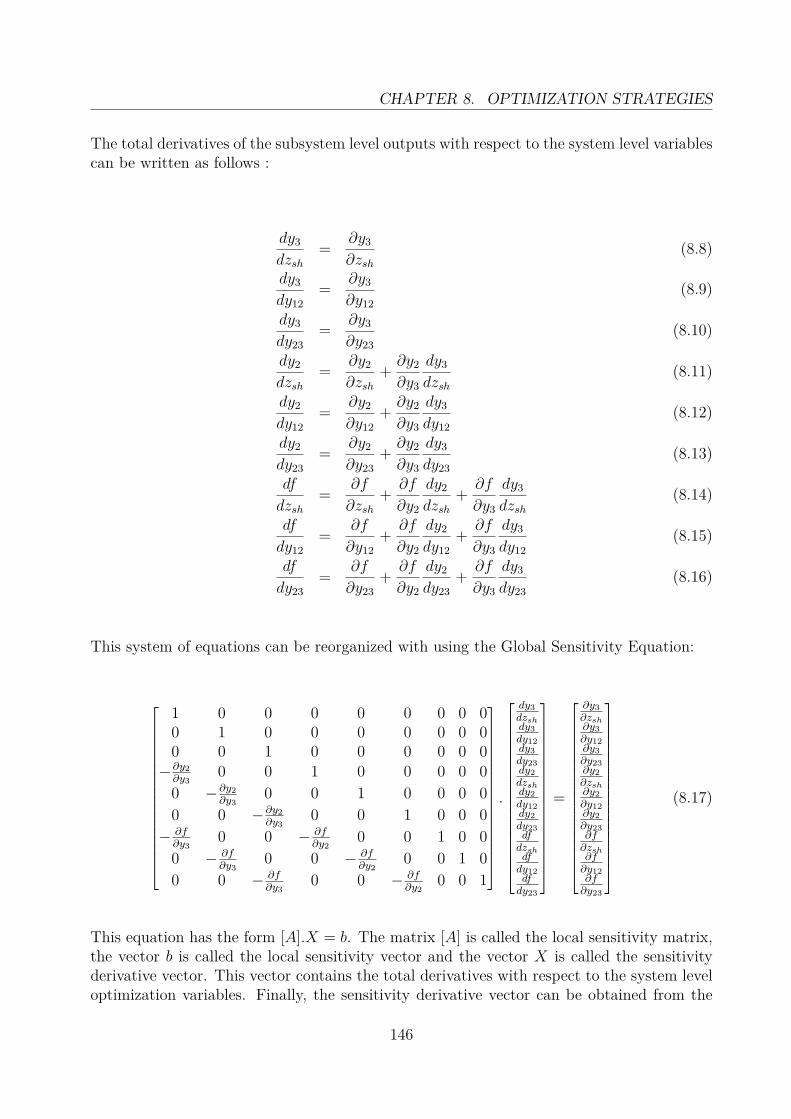
CHAPTER 8. OPTIMIZATION STRATEGIES
The total derivatives of the subsystem level outputs with respect to the system level variablescan be written as follows :
dy3
dzsh= ∂y3
∂zsh(8.8)
dy3
dy12= ∂y3
∂y12(8.9)
dy3
dy23= ∂y3
∂y23(8.10)
dy2
dzsh= ∂y2
∂zsh+ ∂y2
∂y3
dy3
dzsh(8.11)
dy2
dy12= ∂y2
∂y12+ ∂y2
∂y3
dy3
dy12(8.12)
dy2
dy23= ∂y2
∂y23+ ∂y2
∂y3
dy3
dy23(8.13)
df
dzsh= ∂f
∂zsh+ ∂f
∂y2
dy2
dzsh+ ∂f
∂y3
dy3
dzsh(8.14)
df
dy12= ∂f
∂y12+ ∂f
∂y2
dy2
dy12+ ∂f
∂y3
dy3
dy12(8.15)
df
dy23= ∂f
∂y23+ ∂f
∂y2
dy2
dy23+ ∂f
∂y3
dy3
dy23(8.16)
This system of equations can be reorganized with using the Global Sensitivity Equation:
1 0 0 0 0 0 0 0 00 1 0 0 0 0 0 0 00 0 1 0 0 0 0 0 0−∂y2∂y3
0 0 1 0 0 0 0 00 −∂y2
∂y30 0 1 0 0 0 0
0 0 −∂y2∂y3
0 0 1 0 0 0− ∂f∂y3
0 0 − ∂f∂y2
0 0 1 0 00 − ∂f
∂y30 0 − ∂f
∂y20 0 1 0
0 0 − ∂f∂y3
0 0 − ∂f∂y2
0 0 1
.
dy3dzshdy3dy12dy3dy23dy2dzshdy2dy12dy2dy23dfdzshdfdy12dfdy23
=
∂y3∂zsh∂y3∂y12∂y3∂y23∂y2∂zsh∂y2∂y12∂y2∂y23∂f∂zsh∂f∂y12∂f∂y23
(8.17)
This equation has the form [A].X = b. The matrix [A] is called the local sensitivity matrix,the vector b is called the local sensitivity vector and the vector X is called the sensitivityderivative vector. This vector contains the total derivatives with respect to the system leveloptimization variables. Finally, the sensitivity derivative vector can be obtained from the
146

8.5. PHASE III : SECOND OPTIMIZATION PHASE
equation (E.71) by the inversion of the local sensitivity matrix (X = [A]−1.b) :
dy3dzshdy3dy12dy3dy23dy2dzshdy2dy12dy2dy23dfdzshdfdy12dfdy23
=
1 0 0 0 0 0 0 0 00 1 0 0 0 0 0 0 00 0 1 0 0 0 0 0 0−∂y2∂y3
0 0 1 0 0 0 0 00 −∂y2
∂y30 0 1 0 0 0 0
0 0 −∂y2∂y3
0 0 1 0 0 0− ∂f∂y3
0 0 − ∂f∂y2
0 0 1 0 00 − ∂f
∂y30 0 − ∂f
∂y20 0 1 0
0 0 − ∂f∂y3
0 0 − ∂f∂y2
0 0 1
−1
.
∂y3∂zsh∂y3∂y12∂y3∂y23∂y2∂zsh∂y2∂y12∂y2∂y23∂f∂zsh∂f∂y12∂f∂y23
(8.18)
The main advantage of the use of the GSE is the possibility to compute separately the stagesensitivities. It also makes possible the parallelization of the different sensitivity calculations.This calculation technique is explained more in details in Appendix C.
Post-Optimality Analysis
The Post-Optimality Analysis [Sobieszczanski-Sobieski et al., 1982] allows to estimate thegradient of the system level objective function avoiding the reoptimizations of the subsystems(which are required by traditional computation of the gradient using finite differences). Thistechnique has been applied in case of Launch Vehicle Design [Braun et al., 1993] and otheraerospace problems [Sobieszczanski-Sobieski, 1988b; Chandila et al., 2004; Erb, 2007; Martinsand Chittick, 2007; Chittick and Martins, 2008] and allows to enhance the gradient of theobjective function at the system level by adding informations obtained at the subsystemlevel. Let us describe the Post-Optimality Analysis in a simplified case (just one subsystemis considered). Given this assumption, we have at the system level the following optimizationproblem :
Minimize f(z0, z∗1)
With respect to z0
with z∗1 the subsystem level optimized variables obtained during the optimization of thesubsystem. At the subsystem level, the optimization problem can be expressed as follows :
Minimize f(z0, z1)With respect to z1
Subject to e(z0, z1) = 0 (8.19)
For simplification reasons, let us denote by e the equality and saturated inequality constraintsat the point (z0, z
∗1) and ν the corresponding associated Lagrange multipliers vectors. If we
suppose that the set of saturated inequalities (included in e) does not change with respect toa small variation of the system level variables, the system level derivatives can be expressedas follows :
df
dz0(z0, z
∗1) = ∂f
∂z0(z0, z
∗1) + νT
∂e
∂z0(z0, z
∗1) (8.20)
147

CHAPTER 8. OPTIMIZATION STRATEGIES
We can remark that the equation (8.20) allows to compute the system level derivatives di-rectly from the results obtained after the subsystem level optimization. Indeed, for thiscalculation, we have just to evaluate the derivative of the constraints with respect to thesystem level optimization variables, without performing complete reoptimization of the con-sidered subsystems. The different calculations allowing to obtain the equation (8.20) areexplained in details in Appendix C.
Coupled use of the Post-Optimality Analysis and the Global Sensitivity Equation
Replacing the derivatives present in the equations (8.8-8.16) in function of their expressionobtained by using the Post-Optimality Analysis, we have :
dy3
dzsh= ∂y3
∂zsh+ νT3
∂e3
∂zsh(8.21)
dy3
dy12= ∂y3
∂y12+ νT3
∂e3
∂y12(8.22)
dy3
dy23= ∂y3
∂y23+ νT3
∂e3
∂y23(8.23)
dy2
dzsh= ∂y2
∂zsh+ νT2
∂e2
∂zsh+(∂y2
∂y3+ νT2
∂e2
∂y3
)dy3
dzsh(8.24)
dy2
dy12= ∂y2
∂y12+ νT2
∂e2
∂y12+(∂y2
∂y3+ νT2
∂e2
∂y3
)dy3
dy12(8.25)
dy2
dy23= ∂y2
∂y23+ νT2
∂e2
∂y23+(∂y2
∂y3+ νT2
∂e2
∂y3
)dy3
dy23(8.26)
df
dzsh= ∂f
∂zsh+ νT1
∂e1
∂zsh+(∂f
∂y2+ νT1
∂e1
∂y2
)dy2
dzsh+(∂f
∂y3+ νT1
∂e1
∂y3
)dy3
dzsh(8.27)
df
dy12= ∂f
∂y12+ νT1
∂e1
∂y12+(∂f
∂y2+ νT1
∂e1
∂y2
)dy2
dy12+(∂f
∂y3+ νT1
∂e1
∂y3
)dy3
dy12(8.28)
df
dy23= ∂f
∂y23+ νT1
∂e1
∂y23+(∂f
∂y2+ νT1
∂e1
∂y2
)dy2
dy23+(∂f
∂y3+ νT1
∂e1
∂y3
)dy3
dy23(8.29)
Thus, using the same notations as for the GSE, we have the following matrix equation :
1 0 0 0 0 0 0 0 00 1 0 0 0 0 0 0 00 0 1 0 0 0 0 0 0
− ∂y2∂y3
− νT2
∂e2∂y3
0 0 1 0 0 0 0 0
0 − ∂y2∂y3
− νT2
∂e2∂y3
0 0 1 0 0 0 0
0 0 − ∂y2∂y3
− νT2
∂e2∂y3
0 0 1 0 0 0
− ∂f∂y3
− νT1
∂e1∂y3
0 0 − ∂f∂y2
− νT1
∂e1∂y2
0 0 1 0 0
0 − ∂f∂y3
− νT1
∂e1∂y3
0 0 − ∂f∂y2
− νT1
∂e1∂y2
0 0 1 0
0 0 − ∂f∂y3
− νT1
∂e1∂y3
0 0 − ∂f∂y2
− νT1
∂e1∂y2
0 0 1
.
dy3dzshdy3
dy12dy3
dy23dy2
dzshdy2
dy12dy2
dy23df
dzshdf
dy12df
dy23
=
∂y3∂zsh
+ νT3
∂e3∂zzh
∂y3∂y12
+ νT3
∂e3∂y12
∂y3∂y23
+ νT3
∂e3∂y23
∂y2∂zsh
+ νT2
∂e2∂zsh
∂y2∂y12
+ νT2
∂e2∂y12
∂y2∂y23
+ νT2
∂e2∂y23
∂f∂zsh
+ νT1
∂e1∂zzh
∂f∂y12
+ νT1
∂e1∂y12
∂f∂y23
+ νT1
∂e1∂y23
(8.30)
Finally, using the Post-Optimality Analysis and the Global Sensitivity Equation, the system
148

8.6. CONVERGENCE CONSIDERATIONS
level derivatives vector can be expressed as follows :
dy3dzshdy3
dy12dy3
dy23dy2
dzshdy2
dy12dy2
dy23df
dzshdf
dy12df
dy23
=
1 0 0 0 0 0 0 0 00 1 0 0 0 0 0 0 00 0 1 0 0 0 0 0 0
− ∂y2∂y3
− νT2
∂e2∂y3
0 0 1 0 0 0 0 0
0 − ∂y2∂y3
− νT2
∂e2∂y3
0 0 1 0 0 0 0
0 0 − ∂y2∂y3
− νT2
∂e2∂y3
0 0 1 0 0 0
− ∂f∂y3
− νT1
∂e1∂y3
0 0 − ∂f∂y2
− νT1
∂e1∂y2
0 0 1 0 0
0 − ∂f∂y3
− νT1
∂e1∂y3
0 0 − ∂f∂y2
− νT1
∂e1∂y2
0 0 1 0
0 0 − ∂f∂y3
− νT1
∂e1∂y3
0 0 − ∂f∂y2
− νT1
∂e1∂y2
0 0 1
−1
.
∂y3∂zsh
+ νT3
∂e3∂zzh
∂y3∂y12
+ νT3
∂e3∂y12
∂y3∂y23
+ νT3
∂e3∂y23
∂y2∂zsh
+ νT2
∂e2∂zzh
∂y2∂y12
+ νT2
∂e2∂y12
∂y2∂y23
+ νT2
∂e2∂y23
∂f∂zsh
+ νT1
∂e1∂zzh
∂f∂y12
+ νT1
∂e1∂y12
∂f∂y23
+ νT1
∂e1∂y23
(8.31)
This equation allows us to avoid the subsystem reoptimizations to compute the gradientof the system level of the objective function and consequently allows the efficient use ofbi-level gradient-based optimization process in the third phase of the proposed optimizationstrategy.
8.6 Convergence considerationsIn this section, we aim to demonstrate that the third stage-wise decomposition formulationsatisfies the same 1st order KKT conditions as the AAO formulation applied to the stage-wisedecomposition. In order to perform this demonstration, we proceed as follows :
• firstly, we show the equivalence between the 1st order KKT conditions obtained for thefirst SWORD formulation and the conditions obtained with AAO,
• secondly, we show the equivalence between the 1st order KKT conditions obtainedrespectively for the first and the third stage-wise decomposition formulations.
In this section, we only expose the main results of the demonstration. The complete demon-stration of the equivalence between the AAO formulation and the third stage-wise decom-position formulation is given in Appendix D.
The AAO formulation of the optimization problem is the following :
Minimizef(zsh, y, z1, z2, z3) = f1(zsh, y, z1) + f2(zsh, y, z2) + f3(zsh, y, z3)
With respect to zsh, y, z1, z2, z3
Subject to
h1(zsh, y, z1) = 0 (8.32)h2(zsh, y, z2) = 0 (8.33)h3(zsh, y, z3) = 0 (8.34)g1(zsh, y, z1) ≤ 0 (8.35)g2(zsh, y, z2) ≤ 0 (8.36)g3(zsh, y, z3) ≤ 0 (8.37)c01(zsh, y, z2) = 0 (8.38)c02(zsh, y, z3) = 0 (8.39)
149

CHAPTER 8. OPTIMIZATION STRATEGIES
The constraints c01 and c02 can be written as follows :
c01(zsh, y, z2) = f2(zsh, y, z2)− ym1 (8.40)c02(zsh, y, z3) = f2(zsh, y, z3)− ym2 (8.41)
with ym1 and ym2 the two mass components of the coupling vector y.Globally, the demonstration of the equivalence between AAO and the first formulationamounts to show that these two formulations lead to the same set of 1st order KKT condi-tions (Eq. 8.42-8.46). Only the condition concerning the Lagrangian is given here. For thecomplete KKT conditions, one may consult Appendix D.
∂f1
∂zsh+ ∂f2
∂zsh+ ∂f3
∂zsh+ λT
1∂h1
∂zsh+ λT
2∂h2
∂zsh+ λT
3∂h3
∂zsh+ µT
1∂g1
∂zsh+ µT
2∂g2
∂zsh+ µT
3∂g3
∂zsh+ ν1
∂c01
∂zsh+ ν2
∂c02
∂zsh= 0 (8.42)
∂f1
∂y+ ∂f2
∂y+ ∂f3
∂y+ λT
1∂h1
∂y+ λT
2∂h2
∂y+ ΛT
3∂h3
∂y+ µT
1∂g1
∂y+ µT
2∂g2
∂y+ µT
3∂g3
∂y+ ν1
∂c01
∂y+ ν2
∂c02
∂y= 0 (8.43)
∂f1
∂z1+ λT
1∂h1
∂z1+ µT
1∂g1
∂z1= 0 (8.44)
∂f2
∂z2+ λT
2∂h2
∂z2+ µT
2∂g2
∂z2= 0 (8.45)
∂f3
∂z3+ λT
3∂h3
∂z3+ µT
3∂g3
∂z3= 0 (8.46)
The system level equivalence between the first and the third formulations can be shown usingthe Implicit Function Theorem :
Theorem 8.6.1. Implicit Function Theorem[Kudryavtsev, 2001]Let be f : D → R, D ∈ Rn. Let us suppose that ∃ α = (a1, · · · , an) ∈ D and η ∈ R such asf(α) = η and ∂f
∂xn(α) 6= 0,
Then the following hold :
(i) There is a function g(x1, · · · , xn−1), defined near (a1, · · · , an−1) ∈ D ∩ (Rn−1 × {an}),such that
f(x1, · · · , xn−1, g(x1, · · · , xn−1)) = η
(ii) Near α the given equation has no solutions other than the ones described in (i)
(iii) The derivative of g at (a1, · · · , an−1) is given by :
g′(a1, · · · , an−1) =[∂g
∂x1· · · ∂g
∂xn−1
](a1, · · · , an−1) =
− ∂f∂x1
(α)∂f∂xn
(α)· · · −
∂f∂xn−1
(α)∂f∂xn
(α)
By applying this theorem to the first stage-wise decomposition formulation, we can showthat the optimality conditions obtained for this formulation lead to the necessary optimalitycondition of the third formulation :
df
dzF3= 0 (8.47)
150

8.7. CONCLUSION
Concerning the subsystem-level, since the first and third formulations involve the sameoptimization problem for each stage, the subsystem level KKT conditions for the first andthird formulations are the same. Consequently, we can show the equivalence between AAO,first and third formulations about the 1st order KKT conditions. In other words, the optimumfound using the third stage-wise decomposition formulation will also satisfy the optimalityconditions of the AAO formulation, and consequently satisfy the general 1st order optimalitycondition of the MDO problem.
8.7 ConclusionIn this chapter, we have proposed an optimization strategy dedicated to the stage-wise de-composition. This optimization strategy aims to find an optimum in a limited calculationtime and without requiring a priori informations from the user concerning the feasible do-main and the bounds on the optimization variables. This strategy aims to improve theefficiency in terms of calculation time with respect to the global search performed in theprevious part with using a Genetic Algorithm. In this chapter, we have chosen optimizationalgorithms which require the minimal tunings in order to limit as much as possible the in-tervention of the user during the optimization process.
In order to improve the robustness of the optimization process with respect to the startingpoints, we have proposed an automatic initialization process which exploits the stage-wisedecomposition in order to efficiently find feasible designs. These feasible designs are thenused to correctly initialize the optimization phase. The optimization phase is composed oftwo phases, with a first phase which allows to quickly reach the vicinity of an optimum anda second gradient-based phase which aims to quickly converge to the optimum in a limitedsearch space and initialized in the vicinity of the optimum. We propose to use two algorithmsfor the first optimization phase. Indeed, we propose to use firstly a Nelder & Mead algorithmwhich does not require any tuning from the user but may present some difficulties to convergein case of highly non linear search space. If this algorithm is not able to converge or leadsto inconsistent results, we propose to use the Efficient Global Optimization algorithm whichuses Kriging-based response surfaces in order to improve the efficiency (computation time) ofthe optimization process but requires additional points to compute the initial response sur-faces. In the second optimization phase, we use system sensitivity analysis techniques suchas Post-Optimality Analysis and Global Sensitivity Equation in order to avoid the subsystemreoptimizations during the gradient-based search and consequently to save computation time.
In order to validate the different phases of the proposed optimization strategy, a numeri-cal analysis has to be performed in the case of the three-stage launch vehicle MDO problemdefined in Chapter 6. This analysis will also allow us to analyze the efficiency of the opti-mization process (quality of the found optimum, ability to find feasible designs, robustnessto the initialization) and to conclude about the performances of the SWORD method andthe compliance with the requirements defined in the introduction of this chapter.
151


Chapter 9
Analysis of the optimization strategy
Contents9.1 Introduction . . . . . . . . . . . . . . . . . . . . . . . . . . . . . . 1539.2 Determination of the reference design . . . . . . . . . . . . . . . 1549.3 Analysis of phase I : initialization strategy . . . . . . . . . . . . 1579.4 Analysis of phase II : first optimization phase . . . . . . . . . . 158
9.4.1 Comparison of Nelder & Mead and Genetic Algorithm . . . . . . . 1589.4.2 Analysis of the Efficient Global Optimization algorithm . . . . . . 159
9.5 Analysis of phase III : second optimization phase . . . . . . . . 1619.5.1 Accuracy of the gradient estimation . . . . . . . . . . . . . . . . . 1619.5.2 Performance of the proposed gradient-based approach . . . . . . . 161
9.6 Analysis of the whole optimization process . . . . . . . . . . . . 1639.7 Optimization process efficiency . . . . . . . . . . . . . . . . . . . 1669.8 Conclusion . . . . . . . . . . . . . . . . . . . . . . . . . . . . . . . 167
9.1 IntroductionThis chapter is devoted to the numerical analysis of the optimization strategy proposed inthe previous chapter [Balesdent et al., 2011a,b]. Before studying the results obtained for thewhole process, we have to validate each of the proposed optimization phases. To this end,we study each of the different phases separately and compare the results obtained for eachof them.
Concerning the first phase, we compare the results obtained by the proposed initializationprocess with respect to the global random search of all the optimization variables takensimultaneously in order to quantify the computational gain obtained with our proposedstrategy. Concerning the second phase, Nelder & Mead (and Efficient Global Optimization)are compared to a standard Genetic Algorithm from several different initializations. From theresults of this study, we will choose to use either Nelder & Mead or EGO in the global process.Concerning the third phase, we perform 15 different runs from different random feasibleinitializations in the case of restricted search space and we analyze the results obtained bythe proposed bi-level gradient-based algorithm.
After having validated all the different phases, the last section of this chapter concerns the
153

CHAPTER 9. ANALYSIS OF THE OPTIMIZATION STRATEGY
analysis of the whole process. To this end, we generate ten runs of the proposed strategy andwe statistically compare the results obtained for the different generated initializations. Theresults are compared to a reference optimum which has been obtained with fine tunings onthe bounds of the optimization variables and the parameters of the optimization algorithm.
9.2 Determination of the reference designIn order to compare the results obtained in the different phases of the proposed optimizationstrategy, we have to estimate the global optimum design. This optimum has been deter-mined using the third formulation of the SWORD method with a significant initializationwork, the tunings on the bounds of the optimization variables and on the parameters ofthe gradient-based optimization algorithm (we choose a SQP algorithm both at system andsubsystem levels). This tuning phase has required a fine tuning adjustments on the searchspace definition in order to initialize the SQP algorithm in the vicinity of the optimum andto define the bounds on the optimization variables which allow this algorithm to converge.This process has taken several days, and consequently performing the optimization by thisway clearly does not meet the optimization process requirements defined in the previouschapter. Nevertheless, this study is necessary to evaluate the efficiency of our proposedstrategy (quality of the found optimum).From the values of the optimized variables corresponding to the found optimum, we havecalculated the KKT conditions using the MDF formulation and we have verified that thefound optimum effectively satisfies the KKT conditions of the initial problem formulation.The characteristics of the reference optimum are given in Table 9.1. Moreover, the cor-responding optimized trajectory and launch vehicle geometry are given in Figures 9.1 and9.2.
Figure 9.1: Representation of the optimal trajectory
In order to estimate the convexity of the search space around the optimum, some mapshave been calculated in the vicinity of the optimum (Fig. 9.3).
154

9.2. DETERMINATION OF THE REFERENCE DESIGN
Variables Optimum
Propellant mass (t)Mp1 78.3Mp2 26.8Mp3 10.4
Mixture ratioRm1 3.98Rm2 4.11Rm3 4.27
Thrust to weight ratioT/W1 1.82T/W2 1.31T/W3 0.49
Chamber pressure (bar)Pc1 120Pc2 80Pc3 60
Nozzle exit pressure (bar)Pe1 0.42Pe2 4.91.10−2
Pe3 5.54.10−3
Diameter (m)D1 3.61D2 3.61D3 3.61
Maximal load factor nfmax 4.35
Control law 1st stage (◦)
θ11 51.0θ12 37.9θ13 32.4θ14 27.1
Control law 2nd stage (◦)
θ21 18.6θ22 17.2θ23 16.3θ24 11.8
Control law 3rd stage (◦)
θ31 1.00θ32 -6.95θ33 -12.8θ34 -15.0
Altitude at stage separations (km) rf1 61.9rf2 207.9
Velocity at stage separations (km/s) vf1 2.47vf2 5.72
Flight path angle at stage separations (◦) γf1 23.7γf2 7.16
Angle of attack at stage separations (◦) αf1 3.42αf2 4.68
Objective function GLOW (t) 136.68
Table 9.1: Variables for the reference optimum design
155

CHAPTER 9. ANALYSIS OF THE OPTIMIZATION STRATEGY
0 200 400 600 800 10000
100
200
300Altitude
Time (s)
Alti
tude
(km
)
0 500 10000
5000
10000
Velocity
Time (s)
Vel
ocity
(m
.s−
1 )
0 200 400 600 800 1000
0
50
100Flight path angle and pitch angle
Time (s)
Flig
ht p
ath
and
pitc
h an
gles
(°)
Flight path anglePitch angle
0 200 400 600 800 10000
2
4x 10
4 Dynamic pressure
Time (s)
Dyn
amic
pre
ssur
e (P
a)
0 200 400 600 800 10000
2
4
Load factor
Time (s)
Axi
al lo
ad fa
ctor
0 200 400 600 800 10000
5
10
15x 10
4 Mass
Time (s)
Mas
s (k
g)1st stage separation
fairing jettisoning
2nd stage separation
Figure 9.2: Optimal trajectory and geometry
3.55 3.6 3.65 3.73.5
3.55
3.6
3.65
3.7GLOW (t) w.r.t. diameters of the second and third stages
Diameter of stage 3 (m)
Dia
met
er o
f sta
ge 2
(m
)
4.35 4.4 4.45 4.53.5
3.55
3.6
3.65
3.7GLOW (t) w.r.t. maximal load factor and 2nd stage diameter
Maximal load factor
Dia
met
er o
f sta
ge 2
(m
)
206 207 208 209 210
61.7
61.8
61.9
62
62.1
GLOW (t) w.r.t. altitudes of stages separations
Altitude of stage 2 separation (km)
Alti
tude
of s
tage
1 s
epar
atio
n (k
m)
5.68 5.7 5.72 5.74 5.76
2.45
2.455
2.46
2.465
2.47
GLOW (t) w.r.t. velocities of stages separations
Velocity of stage 2 separation (km.s−1)
Vel
ocity
of s
tage
1 s
epar
atio
n (k
m.s
−1 )
136.7
136.8
136.9
137
137.1
137.2
136.7
136.8
136.9
137
137.1
137.2
137.3
137.4
136.7
136.8
136.9
137
137.1
136.7
136.75
136.8
136.85
136.9
136.95
137
Figure 9.3: Evolution of the objective function around the reference optimum
156

9.3. ANALYSIS OF PHASE I : INITIALIZATION STRATEGY
9.3 Analysis of phase I : initialization strategy
In order to quantify the gain expected by using the elaborated initialization strategies, theproposed initialization process has been compared to the standard random search. To thisend, 50000 points have been generated through a randomized process (uniform distribution)in order to statistically compare the methods (Table 9.2). The bounds on the system leveloptimization variables been chosen as very large (Fig. 9.4) and are the same as for the globaloptimization performed in Chapter 6.
0 200 400 600 800 10000
50
100
150
200
250
300Altitude
Time (s)
Alti
tude
(km
)
0 200 400 600 800 10000
2000
4000
6000
8000
10000
12000Velocity
Time (s)
Vel
ocity
(m
.s−
1 )
0 200 400 600 800 1000−20
0
20
40
60
80
100Flight path angle
Time (s)
Flig
ht p
ath
angl
e (°
)
Figure 9.4: Search domain of the position and velocity coupling variables
Random init. Proposed init.Average nb of generated designs required to find a feasible one 4150 244
Proportion of feasible designs in generated population 0.024% 0.41%
Table 9.2: Comparison between global random and proposed initialization process
Using a randomized search on all the optimization variables taken simultaneously, wehave to generate in average 4150 designs to have one feasible design. By using our proposedstrategy, we have to generate only 244 designs to obtain a feasible one that represents about5 minutes of calculation time using MATLAB, 2.4Ghz DualCore Pentium/Windows XP.Consequently, even if the ratio of the feasible designs in the generated population remainsquite low (0.41%), the results show that the proposed initialization process allows to signif-icantly reduce (by a factor 17) the computational cost of the initialization. Moreover, sincethe subsystem databases are increased as the search of feasible designs goes on, the subsys-tem optimizations can be progressively executed more quickly because initialized nearer andnearer to their optimum.
157

CHAPTER 9. ANALYSIS OF THE OPTIMIZATION STRATEGY
9.4 Analysis of phase II : first optimization phase
9.4.1 Comparison of Nelder & Mead and Genetic AlgorithmIn order to validate the choice of the Nelder & Mead algorithm, we have generated differ-ent initializations with the phase I process and for each of them, we have compared theperformance using the Nelder & Mead algorithm with respect to a standard GA. For thiscomparison, we use the same problem formulation and the same initializations. The algo-rithms have been stopped when 400 designs have been generated. Since the Nelder & Meadrequires (n+ 1) initialization points (where n stands for the dimension of the search space),we have to generate 12 designs using the phase I algorithm. Even if the Nelder & Meadalgorithm is more adapted to relatively small search spaces, the comparison is performed ina very large search space, using the same bounds on the optimization variables as in the firstphase (Table 7.4). Nevertheless, all the initialization points are feasible designs.Performing this comparison in a large search space is a good indication to evaluate the abilityof the Nelder & Mead algorithm to converge in our case or the necessity of using a moresophisticated global search algorithm (e.g. EGO, hybridization of Nelder & Mead and GA,globalized Nelder & Mead, etc.).We have generated four complete initializations of 12 (feasible) designs, each of the initial-ization searches taking approximately one hour of calculation time. The results obtained byNelder & Mead and Genetic Algorithm are compared to the reference optimum.
(a) Initialization 1 (b) Initialization 2
(c) Initialization 3 (d) Initialization 4
Figure 9.5: Comparison of Genetic and Nelder & Mead algorithms
Figure 9.5 summarizes the obtained results. For all the considered initializations, we cansee that the Nelder & Mead algorithm obtains better results than the Genetic Algorithm.Indeed, the Nelder & Mead algorithm allows to always find a design less than 0,5t more than
158

9.4. ANALYSIS OF PHASE II : FIRST OPTIMIZATION PHASE
the reference optimum, while the GA presents difficulties to reduce the gap with respectto the reference optimum to less than 1t. Moreover, the different trajectories found by theNelder & Mead algorithm are very close to the reference optimal trajectory, which is not thecase with GA. Figure 9.5 shows the relative contributions of the geometry and the trajectoryto the objective function. For example, in case of the initialization 2, the design found bythe Nelder & Mead algorithm is very close to the reference optimal in terms of geometry butthe trajectory does not exactly match the global optimal one. The opposite phenomenon isobserved for the initialization 1. Concerning the initialization 3, both trajectory and geom-etry of the design found by the Nelder & Mead algorithm match the global optimum ones,that explains the reaching of the optimum.
The Nelder & Mead algorithm appears to be fairly suitable to the SWORD methodbecause it is able to work from the current large search space (whereas a gradient-basedalgorithm cannot be applied). Moreover, it does not need sensitivity calculation during theoptimization process and allows to quickly find a design in the vicinity of the optimum. Asit is shown in Figure 9.5 concerning the first and second initializations, the Nelder & Meadalgorithm may not converged to the true optimum. That reinforces the requirement of agradient-based search in order to refine the obtained design, using the best design found bythe Nelder & Mead algorithm as initialization.
The search space of the actual study case appears to be relatively regular to allow thestandard Nelder & Mead algorithm to quickly find a design in the vicinity of the optimum.That is why we have chosen to select this algorithm in our global optimization strategy.Nevertheless, for other problems (e.g. with a more detailed modelization inducing addi-tional nonlinearities), this algorithm may be inefficient and other global algorithms have tobe considered. In the following subsection, we will test the Efficient Global Optimizationalgorithm which has been selected in the previous chapter.
9.4.2 Analysis of the Efficient Global Optimization algorithmEGO has been compared in the same search space as used in the previous comparisonbetween Nelder & Mead and Genetic Algorithm (Table 7.4) . In order to use EGO, 110feasible designs have been generated using the phase I process. This process has takenapproximately 10 hours of calculation time. Table 9.3 summarizes the tunings of the EGOalgorithm for the current test :
Number of initial points 110θi 10pi 1.75
nuggets 2.10−8
Table 9.3: EGO parameters
Figure 9.6 shows the results obtained using EGO. We can see that EGO is able to obtainsimilar results than Nelder & Mead in only 80 iterations (80 calls to the subsystem level
159

CHAPTER 9. ANALYSIS OF THE OPTIMIZATION STRATEGY
0 10 20 30 40 50 60 70 80 90137
137.5
138
138.5
139
139.5
140
140.5
141Global optimization via EGO
GLO
W(t
)
Number of generated designs
Figure 9.6: Results obtained with EGO
optimizations). Indeed, EGO requires only 20% of the number of iterations involved bythe Nelder & Mead algorithm in the previous section but needs more initialization points.Even if EGO allows to obtain interesting results, we have not selected this algorithm in ouroptimization strategy because :
• it appears that the Nelder & Mead algorithm is sufficient in our study case,
• EGO requires more tunings (tunings on the Kriging model parameters) than the Nelder& Mead algorithm, and consequently appears to be less adapted because of the factthat one of the requirement of the optimization process is to have lesser interventionof the user (the user does not have a priori knowledge of the fine tunings on theoptimization algorithm),
• this algorithm requires a great number of initial feasible designs in order to build theresponse surfaces, which induces an important calculation time (110 feasible designstake 10 hours of computation time using the phase I initialization process, whichsubstantially debases the efficiency of the optimization process),
Some studies have been performed with less than 110 points to compute the initialresponse surface (25 and 55 points) but lead to inconsistent results. Nevertheless, the ap-proximation by Kriging is a cheaper approach which is adapted in our case in order to realizethe maps of the objective function around the optimum (Fig. 9.7).
160

9.5. ANALYSIS OF PHASE III : SECOND OPTIMIZATION PHASE
vf2 (km.s−1)
vf1 (
km.s
−1 )
Std. dev. of the prediction error and sample points
5.68 5.7 5.72 5.74 5.76
2.45
2.455
2.46
2.465
2.47
Estimation by kriging (50 points)
vf2 (km.s−1)
vf1 (
km.s
−1 )
5.68 5.7 5.72 5.74 5.76
2.45
2.455
2.46
2.465
2.47
vf1 (
km.s
−1 )
vf2 (km.s−1)
Real objective function (2500 points)
5.68 5.7 5.72 5.74 5.76
2.45
2.455
2.46
2.465
2.47
rf2 (km)
rf1 (
km)
Std. dev. of the prediction error and sample points
206 207 208 209 21061.6
61.7
61.8
61.9
62
Estimation by kriging (50 points)
rf2 (km)
rf1 (
km)
206 207 208 209 21061.6
61.7
61.8
61.9
62
rf1 (
km)
rf2 (km)
Real objective function (2500 points)
206 207 208 209 210
61.7
61.8
61.9
62
62.1
nf
D2
(m)
Std. dev. of the prediction error and sample points
4.35 4.4 4.45 4.53.5
3.55
3.6
3.65
3.7Estimation by kriging (50 points)
nf
D2
(m)
4.35 4.4 4.45 4.53.5
3.55
3.6
3.65
3.7
D2
(m)
nf
Real objective function (2500 points)
4.35 4.4 4.45 4.53.5
3.55
3.6
3.65
3.7
D3 (m)
D2
(m)
Std. dev. of the prediction error and sample points
3.5 3.55 3.6 3.653.5
3.55
3.6
3.65
Estimation by kriging (50 points)
D3 (m)
D2
(m)
3.5 3.55 3.6 3.653.5
3.55
3.6
3.65
D2
(m)
D3 (m)
Real objective function (2500 points)
3.5 3.55 3.6 3.65 3.73.5
3.55
3.6
3.65
3.7
0.02
0.04
0.06
0.08
136.7
136.8
136.9
137
137.1
136.8
137
137.2
136.8
137
137.2
137.4
136.8
137
137.2
137.4
0.05
0.1
0.15
0.01
0.02
0.03
136.7
136.8
136.9
137
137.1
136.7
136.8
136.9
137
137.1
136.7
136.8
136.9
137
136.7
136.8
136.9
137
0.005
0.01
0.015
0.02
Figure 9.7: Real map (2500 points) and kriged maps (50 points) around the optimum
9.5 Analysis of phase III : second optimization phase
9.5.1 Accuracy of the gradient estimationIn order to validate the gradient estimation, we have computed the sensitivities with Post-Optimality Analysis (POA) and Global Sensitivity Equation (GSE), and using classical finitedifferences (Table 9.4). The coupled use of POA and GSE allows to divide the computationtime of the sensitivity calculation phase by 434, for a maximal error of approximately 1%,which is very satisfactory in our case.
9.5.2 Performance of the proposed gradient-based approachIn order to validate the proposed gradient-based approach, we have generated randomly15 initializations in the vicinity of the optimum. The optimization has been restricted toa search domain corresponding to 2% of the optimization variable dynamics around thereference optimum. Table 9.5 summarizes the results obtained for each of the initializations.Globally, the proposed algorithm allows to obtain in average a GLOW of 136,7t from aninitial GLOW of 137.7t in average.
161

CHAPTER 9. ANALYSIS OF THE OPTIMIZATION STRATEGY
Finite Differences (FD) POA+GSE Relative difference betweenFD and POA+GSE
∂f∂D2
−2.42942.102 −2.42359.102 0.24%∂f∂D3
−1.36954.103 −1.37620.103 0.48%∂f∂nf 1.87916.103 1.89293.103 0.73%∂f∂rf2
2.40695.102 2.42533.102 0.76%∂f∂vf2
4.04506.103 4.06896.103 0.59%∂f∂γf2
4.62184.102 4.66507.102 0.93%∂f∂αf2
2.52984.102 2.52868.102 0.05%∂f∂rf1
2.02675.102 2.04431.102 0.86%∂f∂vf1
−1.20073.103 −1.19255.103 0.69%∂f∂γf1
−5.05289.102 −5.02531.102 0.55%∂f∂αf1
−1.06994.102 −1.07330.102 0.31%Calculation time (s) 582 1.34
Table 9.4: Accuracy of the gradient estimation
Indeed, the bi-level gradient-based optimization algorithm allows to find the optimum withan average error of 0.1%, which a satisfactory error rate in the early phase studies becauseit is lower than the accuracy of our models. Moreover, in 5 of the 15 cases, the algorithmallows to exactly reach the reference optimum. Consequently, the results obtained for thistest allow to validate the proposed optimization process.
Init.(t) ∆init Found(t) ∆opt Nb iter Improvement ∆1 137.90 0.89% 136.81 0.09% 8 -89.61%2 137.11 0.31% 136.73 0.04% 4 -88.29%3 137.50 0.60% 136.72 0.03% 12 -95.46%4 137.89 0.89% 136.76 0.06% 7 -93.55%5 137.68 0.73% 136.68 0.00% 20 -100%6 137.19 0.37% 136.82 0.10% 3 -71.79%7 137.58 0.66% 136.68 0.00% 7 -100%8 137.85 0.86% 136.88 0.15% 9 -82.75%9 138.23 1.13% 136.91 0.17% 7 -84.71%10 138.01 0.97% 136.89 0.15% 8 -84.48%11 137.10 0.31% 136.68 0.00% 7 -100%12 138.24 1.14% 136.68 0.00% 14 -100%13 137.19 0.37% 136.68 0.00% 6 -100%14 138.81 1.56% 136.84 0.11% 4 -92.62%15 137.46 0.57% 136.78 0.07% 6 -86.92%
Average 137.72 0.76% 136.77 0.09% 8.3 -91.35%Std deviation 0.49 0.36% 0.09 0.09% 0.06 8.35%
Table 9.5: Results obtained for the validation of the second optimization phase
162

9.6. ANALYSIS OF THE WHOLE OPTIMIZATION PROCESS
In this section, we have analyzed all the different phases of the proposed optimizationstrategy. This analysis has been performed taking into account the different phases sepa-rately. In the next section, we analyze the whole optimization process in order to study ifthe proposed optimization strategy meets the optimization requirements or not.
9.6 Analysis of the whole optimization processIn order to analyze the whole optimization process, we have chosen to perform 10 optimiza-tions. For that purpose, 10 automatic searches of feasible designs have been performed.Then, from these designs, we have launched 10 times the Nelder & Mead algorithm and fi-nally, from the designs found by this algorithm, we have launched the bi-level gradient-basedoptimization process. Let us describe the results obtained for the three phases.Table 9.6 summarizes the results obtained in the phase I. In this table are represented thebest design of each initialization (each initialization regroups 12 feasible designs), the numberof generated designs required to find 12 feasible designs and the percentage of success. Theresults present in this table are consistent with respect to the analysis of the phase I exposedpreviously. Figure 9.8 summarizes all the designs found during the phase I (in terms ofrelative difference with respect to the reference optimum). All the feasible designs obtainedafter phase I are represented in the left colored bars. This phase takes approximately onehour.
N◦ init. Best design Generated designs Success rate1 140,87t 2820 0.42%2 145,07t 3145 0.38%3 141,22t 3532 0.33%4 140,13t 2472 0.48%5 140,22t 1678 0.71%6 143,72t 4417 0.27%7 139,47t 2318 0.51%8 140,87t 3274 0.37%9 142,88t 3533 0.34%10 142,84t 2668 0.45%
Table 9.6: Results obtained for the phase I
The results obtained during the phase II are summarized in Table 9.7. In this table areindicated the best design found during the phase I, the best design found by the phase IIalgorithm and the number of expended points during the process. The results obtained inthis phase are represented in Figure 9.8 (middle bars). This process takes between one andtwo hours and achieves the main part of the optimization.
163

CHAPTER 9. ANALYSIS OF THE OPTIMIZATION STRATEGY
N◦ init. Best design of init Best design found by N&M Nb of iterations1 140,87t 137,58t 3222 145,07t 137,08t 3773 141,22t 137,04t 2004 140,13t 137,03t 2375 140,22t 137,18t 1606 143,72t 136,86t 2617 139,47t 137,14t 2888 140,87t 138,11t 3109 142,88t 137,46t 26010 142,84t 137,04t 314
Table 9.7: Results obtained for the phase II
Finally, from the best design found by the phase II process, the gradient-based bi-level op-timization process performs the optimization in the estimated vicinity of the optimum. Theresults obtained during the phase III are given in Table 9.8. In this table are indicated thebest designs, the relative differences with respect to the reference optimum and the numbersof system level iterations. The numbers of subsystem level optimizations are given in paren-thesis. These numbers are higher than the numbers of iterations because the optimizationalgorithm at the system level involves a step size calculation which is performed at eachiteration and requires a few calculations of the objective function and consequently a fewsubsystem level optimizations. The results obtained after the third phase are represented asthe right bars in Figure 9.8. Table 9.9 summarizes the results obtained by the whole process.
N◦ init. Init Best design found Diff. vs opt. Nb of iterations (subsystem opt.)1 137,58t 136,91t 0.16% 25(98)2 137,08t 136,89t 0.15% 7(19)3 137,04t 136,70t 0.01% 11(98)4 137,03t 136,94t 0.19% 5(75)5 136,97t 136,90t 0.16% 17(58)6 136,86t 136,81t 0.10% 8(88)7 137,14t 136,94t 0.19% 9(94)8 138,11t 136,94t 0.19% 22(128)9 137,649t 136,83t 0.11% 8(35)10 137,04t 136,78t 0.07% 10(98)
Table 9.8: Results obtained for phase III
164

9.6. ANALYSIS OF THE WHOLE OPTIMIZATION PROCESS
N◦ init. Diff. w.r.t. opt. Reduction of gap w.r.t. Total computation timebest initial design1 0.16% -94.51% 4h072 0.15% -97.50% 3h003 0.01% -99.67% 3h424 0.19% -93.35% 3h105 0.16% -93.72% 3h166 0.10% -98.18% 4h357 0.19% -90.57% 4h308 0.19% -93.87% 4h549 0.11% -97.63% 3h4210 0.07% -98.34% 4h16
Average 0.14% -95.76% 3h55Standard deviation 0.06% 2.89% 39min
Table 9.9: Summary of the results
Figure 9.8 presents the evolution of the relative difference (in percentage) between thebest found design and the reference optimum (which is obtained with fine tunings on theoptimizers and design variable variation domains). The different divisions of colored left barsrepresent the 12 feasible designs obtained after phase I, which are used to initialize the firstoptimization phase. In all cases, the optimization process converges with a maximal relativegap of 0.2% between the found design and the reference optimum. Indeed, the relativedistance between the found design and the reference optimum is reduced by 96% (Fig. 9.8)on average in a calculation time of approximately 4 hours using MATLAB, 2.4GHz DualCorePentium/Windows XP. Figure 9.9 illustrates the phase III algorithm behavior for the thirdrun. We can see that the algorithm converges to the optimum in 11 iterations (calculationtime : approx. 90min).
1 2 3 4 5 6 7 8 9 100123456789
10111213141516171819202122232425262728
Runs
Diff
eren
ce w
.r.t.
ref
eren
ce o
ptim
um (
%)
Study case synthesis
Feasible points found during phase I
Best point found during phase II
Best point found during phase III
Figure 9.8: Synthesis of the results obtainedfor the different phases
Dia
met
er o
f sta
ge 2
(m
)
Diameter of stage 3 (m)
GLOW (t) w.r.t. diameters of the second and third stages
1
2
345− 6
7
8−1011
3.5 3.55 3.6 3.65 3.73.5
3.52
3.54
3.56
3.58
3.6
3.62
3.64
3.66
3.68
3.7
136.7
136.75
136.8
136.85
136.9
136.95
137
Figure 9.9: Example of phase III algo-rithm’s behavior
165

CHAPTER 9. ANALYSIS OF THE OPTIMIZATION STRATEGY
136
137
138
139
140
141
142
143
144
145
146
Phases
GLO
W (
t)Objective function evolution during the different phases
PHASE I PHASE II PHASE III
Reference optimum
di
dopt
Figure 9.10: Evolution of the objective func-tion during the optimization process
Maximum distance between the5.59tdifferent initializations di
(best designs of phase I)Maximum distance between 0.25tthe found optima doptdopt/di 4.44%
Table 9.10: Dispersion of the founddesigns
In order to quantify the robustness of the algorithm, defined here as the ability to convergefrom large search space, we have compared the dispersion of the 10 found designs relatively tothe one of the initializations found after phase I (Tab. 9.10 and Fig. 9.10). The results showthat the proposed strategy presents satisfactory robustness properties because the dispersionof the found designs is just 4.44% of the initialization one.
Remark 9.6.1. Even if the EGO al-gorithm has not been selected for theproposed optimization strategy, wehave performed the bi-level gradient-based optimization from the designfound by the EGO algorithm (Fig.9.6). The results indicate that theinitialization provided by EGO al-lows the convergence of the gradient-based algorithm with a relative errorof 0.1% to the optimum, which is inthe same order of magnitude as theresults found when the gradient-basedalgorithm is initialized by Nelder &Mead (Fig. 9.11).
0 50 100 150 200 250
136
137
138
139
140
141
142Global optimization via EGO
GLO
W(t
)
Number of generated designs
EGO
Gradient−based optimization
Reference optimum
∆=0.1%
Figure 9.11: Evolution of the objective func-tion during the optimization using EGO andgradient-based algorithm
9.7 Optimization process efficiencyTo conclude about the efficiency of the proposed strategy, let us analyze the results obtainedby using the proposed optimization process with respect to the optimization requirementsexpressed in the previous chapter :
166
9.8. CONCLUSION
1. "ability to quickly find feasible designs from random initialization" :The search of feasible designs is performed in a dedicated phase. The feasible designsare computed without any action of the user. The numerical results show that theproposed process is able to find a feasible design in approximately 5 minutes. Conse-quently, the initialization phase takes approximately one hour, instead of more than10 hours with a global random search. From this point of view, the proposed processis relatively efficient and allows to meet the requirement.
2. "robustness to the initialization" :In order to quantify the robustness of the optimization process, we have performed tenruns of the optimization process. Even if the feasible designs found after the phaseI are scattered all along the search space, the results found after phase III are veryclose. Indeed, the dispersion of the found designs is just 4.44% of the dispersion of thefeasible designs. This characteristic is a good indicator to evaluate the robustness ofthe optimization process and shows that the proposed strategy meets the robustness(stability) requirement fairly well.
3. "ability to converge from very large search domains" :One of the principal requirement for our proposed strategy is the ability to work ina very large search space. From this point of view, the proposed algorithm allowsto initially work on very large search space and reduces the search space during theoptimization process in order to more efficiently converge toward the optimum. Thus,this decomposition of the optimization process in three phases in which each phase isdevoted to a particular task allows to meet the large search space convergence abilityrequirement.
4. "once the feasible domain is reached, the ability to efficiently converge toward an op-timum":The decomposition of the optimization process into two phases (Nelder & Mead orEGO and bi-level gradient-based algorithms) allows to exploit the advantages of eachof the used optimization algorithms and consequently allows to converge with a max-imal difference of 0.2% with respect to the reference optimum. This optimization isperformed into approximately 3 hours which is quite satisfactory, taking into accountthe required time by a classical global search as performed in Chapter 7.
9.8 ConclusionThe works presented in this part concern the elaboration of an optimization strategy dedi-cated to the SWORD method (and more particularly the third formulation of the SWORDmethod). For this purpose, we have created an optimization process which allows to per-form in a limited calculation time (a few hours) the optimization in case of a large searchspace without a priori knowledge on the optimization variable variation domains and withlimiting at the most the action of the user. These different requirements have brought us toperform the optimization and exploration tasks separately. Indeed, decomposing these twotasks makes possible the use – or the creation if necessary – of dedicated algorithms for each
167

CHAPTER 9. ANALYSIS OF THE OPTIMIZATION STRATEGY
of them and consequently improves the efficiency of the whole process.
Since the initial search space is very large and the feasible domain cannot be known inadvance, we have chosen to develop an exploration strategy based on a series of the explo-rations of the system level variables relating to the different stages. Thus, this exploratorysearch allows to save computational time with respect to the exploration of all the systemlevel optimization variables taken simultaneously and therefore appears to be a computa-tionally efficient way to find a consistent (feasible) initialization for the optimization phase.
Moreover, we have chosen to split up the optimization phase into two phases. This allowsto improve the flexibility of the optimization process and to leave the user free to use in thefirst optimization phase a global optimization algorithm if the search space is too highly nonlinear and presents multiple optima or if the classical Nelder & Mead algorithm, which isused by default, is not able to find consistent results. Once the first phase optimization isachieved and the vicinity of an optimum (expected as global) is reached, we have chosento use a gradient-based algorithm in which we have replaced the classical finite differencesensitivity calculation by an estimation using the Post-Optimality Analysis, which allows tosave a great computational time at the cost of reasonable approximation errors.
Each of the phases of the proposed optimization strategy has been separately testedin order to validate its behavior and a global analysis of the whole proposed optimizationstrategy has been performed. In order to quantify the robustness of the process and tohave a statistical idea of the strategy comportment, we have performed 10 optimizations,from random initializations found by the exploratory algorithm. The results show that theoptimization process allows to get closer to less than 0.2% to the reference optimum, ina calculation time less than 4 hours. These results are relatively satisfactory taking intoaccount that this process is intended to be used in early phase studies in which simplified(and therefore not accurate) models are used (the relative difference between the obtainedoptima and the reference optimum is below the precision of the models).
168

Conclusion and perspectives
This thesis is focused on the development of MDO methodologies devoted to preliminaryLaunch Vehicle Design studies. Our contribution is the development of new MDO formu-lations, called SWORD (Stage-Wise decomposition for Optimal Rocket Design), exploitinga transversal decomposition of the design process according to the different flight phases ofthe launch vehicle. The SWORD formulations allow to distribute the problem complexityamong the system and the subsystem optimization levels and to transform the initial globaloptimization problem into the coordination of a series of elementary subproblems which canbe solved more easily.
From the analysis of the application of the different existing MDO methods to LVD,we have proposed a new formulation of the LVD MDO problem focused on the trajectoryoptimization and reflecting the physical architecture of launch vehicles. To this end, wehave developed four MDO formulations and have compared them with the MDF method incase of global search study. The results of this study have shown that two of the proposedformulations (collaborative and non hierarchical) stand out from all the others and allowto improve the efficiency of the optimization process with respect to the commonly-usedmethod in LVD (MDF), in terms of calculation time to find a feasible design from randominitialization and quality of the found design for a given computation time. Therefore, withan appropriate formulation, the stage-wise decomposition makes the global search algorithmsmore efficient to solve the LVD problem from random initializations and without requiringspecific knowledge of the optimization variable variation domains. Nevertheless, this studyhas shown that the use of a global search alone is not sufficient to obtain an optimum inan acceptable calculation time (a few hours). Therefore, the development of a specific opti-mization strategy is necessary.
In the second part of this thesis, we have proposed an optimization strategy dedicatedto the stage-wise decomposition. To this end, we have used the non hierarchical SWORDformulation in order to propose an optimization strategy which aims to quickly find feasibledesigns, to converge to an optimum in a limited calculation time, to perform the optimiza-tion on a very large search space (in terms of optimization variable variation domains) andto improve the robustness to the initialization. In order to meet these requirements, we haveproposed a three-phase optimization strategy.
The first phase is inspired by the non hierarchical SWORD formulation and consists of asequential exploration of the different system level optimization variable subsets interveningin the different flight phases of the launch vehicle. This method allows to considerably reducethe computation time to find feasible designs with respect to a global random exploration
169

CONCLUSION
of all the optimization variables at the same time.From the feasible designs found during the first phase, we have chosen to perform the
optimization in two steps. The first step involves a gradient-free optimization using theNelder & Mead algorithm (or the Efficient Global Optimization algorithm if the searchspace is highly non linear) in order to quickly reach the vicinity of an optimum. Finally,from the best design found during the first optimization step, the second step consists inperforming a gradient-based optimization at the system level, in a limited search space inthe vicinity of the optimum. In order to reduce the computation time of this phase, wehave replaced the classical finite difference computation of the gradient of the system levelobjective function by an estimation which does not require any time-costly subsystem re-optimizations. This estimation is performed using dedicated calculation techniques whichexploit the convergence informations given by the subsystems (Post Optimality Analysis andGlobal Sensitivity Equation).
A global analysis of the whole process (formulation and optimization strategy) has thenbeen achieved in order to evaluate the performance of the SWORD method. The resultsshow that the optimization process allows to get closer to less than 0.2% to the referenceoptimum, in a calculation time less than 4 hours, that is satisfactory for early design studiesin comparison with classical approaches which take more than 10 hours when performed insuch a large search space. This analysis has validated the proposed optimization strategyand has shown that the use of the stage-wise decomposition is valuable in order to solve inlimited calculation time the LVD problem without requiring a priori knowledge of the user.
In order to improve the proposed MDOmethod, some extensions of the works presented inthis thesis can be proposed. The described design process is currently devoted to early designstudies in which simplified models are used. It would be interesting to test the proposedmethod with more complicated disciplinary models, involving additional couplings.
Moreover, in this thesis, we have compared the SWORD methods with MDF and notwith other MDO methods such as BLISS, ATC, CSSO, etc. The comparison of the SWORDmethods with these MDO methods would be very interesting but requires to build moredetailed disciplinary models in order to be able to apply the MDO methods present inliterature.
Additionally, as the SWORD method is principally devoted to early design studies inwhich simplified models are used, it would be valuable to incorporate the handling of modeluncertainties in the current design process in order to ensure the consistency of the designduring the following phases of the design process.
Furthermore, the optimal control method involved in this thesis is a direct method. Itwould be interesting to study in future works other trajectory optimization methods (e.g.indirect method) in order to choose the most adapted to the design process.
In addition, the SWORD method has been tested on the design problem of classicalexpendable launch vehicles with sequential staging (no booster). It would be very helpful totranspose and test the SWORD formulations to more complex launch vehicle design problemssuch as the launch vehicles with parallel staging or the reusable launch vehicles. In the samemanner, the current design process is only able to handle continuous optimization variables.The introduction of discrete variables would be valuable and would allow to consider in thedesign process other characteristics of launch vehicles such as the number of stages, etc.
170

Finally, in this thesis, we have applied the SWORD method to single objective problems.It would be also interesting to test our method in case of multi objective problems (e.g. themaximization of the payload and the minimization of the cost). This study case would allowus to design a family of optimal launch vehicles and to be able to propose several choices oflaunch vehicles for different missions.
171


Appendix A
Dry mass sizing module
The dry mass sizing module aims at calculating the dry mass of the launch vehicle in orderto compute the objective function and to simulate the trajectory. The dry mass of each stageis the sum of the main launch vehicle components :
• tanks,
• turbopumps,
• pressurant system,
• combustion chamber,
• nozzle,
• engine.
A.1 Tanks
Tanks sizing module
Me
Rm M tanks
D
Figure A.1: Tank sizing module
Selected material : Aluminium.Properties of aluminium :
Density(ρAl) 2800kg.m−3
Ultimate strength (σrAl) 400 MPaYield strength (σeAl) 380 MPa
Minimal thickness (eminAl) 1.5 mm
Fixed parameters :
173

APPENDIX A. DRY MASS SIZING MODULE
• Safety coefficient (Cs) : 1.25
• Margin of safety for the tank’s thickness (fR) : 1.2
Inputs :
• Mp : propellant mass (kg)
• Rm : mixture ratio
• D : stage diameter (m)
Determination of the tank volume:
From Mp and Rm, we determine the propellant volumes by :
VLOX = 1ρLOX
Mp.Rm
Rm+ 1 (A.1)
VH2 = 1ρH2
Mp
Rm+ 1 (A.2)
with :
• ρLOX = 1141 kg.m−3
• ρH2 = 71 kg.m−3
Tank pressures : The tank pressures are given by the following expressions [Humble et al.,1995] :
PrLOX = [10−0.1068.log(VLOX)−0.2588106.].106 (A.3)PrH2 = [10−0.1068.log(VH2)−0.2588106 ].106 (A.4)
Tanks thickness :
erLOX = Cs.PrLOX .DR
2σrAl(A.5)
erH2 = Cs.PrH2 .DR
2σrAl(A.6)
The considered tanks are two cylinders provided with spherical bulkheads. The radius ofthe spherical bulkhead is given in function of the tank’s diameter by the following formula :
Rc = DR
2 (A.7)
The volume of the tank is given by :
VR = π.(DR
2
)2LR + 4
3π(DR
2
)3(A.8)
174

A.2. TURBOPUMPS
From Equation A.8, we can determine the length (cylinder part) in function of its radiusand its volume. Therefore, the surface of the tank is given by :
SR = π.DR.LR + 4π(DR
2
)2(A.9)
Thus, the mass of the tank is :
Mtank = eR.SR.fR.ρAl (A.10)
By replacing LR by its expression in function of DR and VR (so D andMp from the equationsA.1 and A.2) the mass of the tanks can be calculated.
A.2 TurbopumpsInputs :• Pc : chamber pressure (Pa)
• q : mass flow rate (kg/s)
• Rm : mixture ratio
• Mp : propellant mass (kg)
Turbopumpssizing module
Pc
q
M TP
Rm
Me
Figure A.2: Turbopumps sizing module
The mass flow rate of LOX and LH2 are given by :
qLOX = qRm
1 +Rm(A.11)
qH2 = q1
1 +Rm(A.12)
From the difference of pressure between the tanks and the combustion chamber, the massflow rate, the density of the fluid and the efficiency of the pump (ηP = 75%), we determinethe necessary power of the pump :
PWLOX/H2 = qLOX/H2(Pc− PrLOX/H2)ρLOX/H2.ηP
(A.13)
Then, the mass of the turbopump is given by [Humble et al., 1995] :
MTPLOX/H2 = 1.5(PWLOX/H2
2Nπ/60
)0.6
(A.14)
with N the rotational speed of the pump (12400 tr/min).
175

APPENDIX A. DRY MASS SIZING MODULE
A.3 Pressurant systemInputs :
• Mp : propellant mass (kg)
• Rm : mixture ratio
Pressurant systemsizing module
M pressRm
Me
Figure A.3: Pressurant system sizing module
Data :
• Initial gas temperature (T0) : 300k
• Pressurant gas : helium He
• Initial pressure in the pressurant tank (P0) : 200 bars
• Final pressure in the pressurant tank (Pf ) : 120%max(PrLOX , PrH2)
• Ratio of specific heats for the pressurant gas (γHe) : 1.67
• Molecular mass of the pressurant gas (MHe) : 0.004 kg/mol
• Mass density of the pressurant tank material (ρcapa) : 1570 kg.m−3
• Tensile strength of pressurant tank material (σr) : 1270 MPa
• Safety coefficient Cs : 2
• Thickness of the liner (density ρliner : 2800 kg/m3) (eliner) : 1mm
The volume of the pressurant tank is given by :
V0 = max(PrLOX , PrH2)γHe.VRP0 − Pf
(A.15)
The mass of the pressurant gas is calculated by :
mHe = MHe.P0.V0
R.T0(A.16)
with R=8.314 ISU, the pressurant gas constant.The inner radius of the pressurant tank is given by :
Rint =(3.V0
4π
) 13
(A.17)
176

A.4. COMBUSTION CHAMBER
We define the thickness of the tough material by :
er = Cs.P0.Rint
2.σr(A.18)
The total thickness is :etot = eliner + er (A.19)
The outer radius of the pressurant tank is given by :
Rext = etot +Rint (A.20)
Finally, the mass of the pressurant tank (overestimated by 10%) is :
mc = 1.143π(((R3
ext − (Rint + eliner)3)ρcapa + ((Rint + eliner)3 −R3int)ρliner) (A.21)
Then the total mass of the pressurant system is given by :
Mpress = mHe +mc (A.22)
A.4 Combustion chamberInputs :
• Pc : chamber pressure (Pa)
• Rm : mixture ratio
• q : mass flow rate (kg/s)
Combustion chambersizing module
Pc
Rm M ch
q
Figure A.4: Combustion chamber sizing module
The isentropic coefficient (γ), the flame temperature (Tc), and the molecular mass ofcombustion (M) are interpolated from classical curves found in [Humble et al., 1995] (fig.A.5) The cross-sectional area of nozzle throat is given by :
Ac = q√γ.R.Tc
ηc.P c.γ(
2γ+1
) γ+12γ−2
(A.23)
with ηc the combustion efficiency (0.98), R the gas constant 8314M
.The throat’s diameter is :
Dc = 2√Acπ
(A.24)
177

APPENDIX A. DRY MASS SIZING MODULE
3 4 5 61.2
1.21
1.22
1.23
1.24
1.25
1.26
Mixture ratio
Isen
trop
ic c
oeffi
cien
t (γ t)
Isentropic coefficient (γt)
3 4 5 62400
2600
2800
3000
3200
3400
3600
Mixture ratio
Fla
me
tem
pera
ture
(T
c)
Flame temperature (Tc)
3 4 5 68
9
10
11
12
13
14
Mixture ratio
Mol
ecul
ar m
ass
of c
ombu
stio
n (k
g/km
ol)
Molecular mass of combustion (Mc)
Figure A.5: Propulsive parameters
We have the following relationship between the cross-sectional area of nozzle throat and thethroat’s diameter :
Ach = (8(100Dc)(−0.6) + 1.25)πD2c
4 (A.25)
The diameter of the chamber is given by :
Dch = 2√Achπ
(A.26)
The length of the chamber is given by :
Lch = L∗(Dc
Dch
)2(A.27)
with L∗ the characteristic length (1.02 for the couple LOX/LH2). The thickness of thechamber is given by :
ech = Pc.fpDch
2σch(A.28)
with σch = 310MPa the tensile strength of the chamber material, fp = 2 a safety coefficientand ρch = 8000kg.m−3 the density of the chamber material.Finally, the mass of the chamber is given by :
Mch = (2.Ach + πDchLch)echρch (A.29)
A.5 NozzleInputs :
• Pc : chamber pressure (Pa)
• Pe : exit pressure (Pa)
• Rm : mixture ratio
178

A.6. ENGINE
Nozzle sizing module
Pc
Ps M n
Rm
Figure A.6: Nozzle sizing module
The nozzle expansion ratio is given by :
ε =
(2
γ+1
) 1γ−1 .Pc
Ps
1γ√√√√(γ+1
γ−1
).
(1−
(PsPc
) γ−1γ
) (A.30)
The nozzle throat area is :An = Acε (A.31)
Then, the nozzle exit diameter is given by :
Dn = 2√Anπ
(A.32)
The conical nozzle length (with a nozzle cone half angle of 15◦) is :
LN = Dn −Dc
2. tan(15π/180) (A.33)
Thus, the nozzle length is :Ldiv = LN.λ (A.34)
The thickness of the nozzle inner structure is given by :
en = 0, 5.P c.Dc.fn2σrn
(A.35)
with fn a safety coefficient (fn = 2) and σrn = 310MPa the ultimate strength of the nozzlematerial. Finally, the nozzle mass is given by (with ρn = 8000kg.m−3) :
Mn = πρn.en.Ldiv(Dn +Dc)2 (A.36)
A.6 EngineThe engine is calculated from the masses of the nozzle and the combustion chamber by thefollowing relationship [Humble et al., 1995] :
Meng = Mn +Mch
ξ(A.37)
with :
179

APPENDIX A. DRY MASS SIZING MODULE
• ξ = 0.2 si Pc ≤ 20 bars
• ξ = 0.230 Pc+ (0.6− 500.2
30 ) if 20bars≤ Pc ≤ 50bars
• ξ = 0.4 else
A.7 Offset mass for models adjustmentAt this level, the dry mass model underestimates the real dry mass of the existing cryogenicstages found in ESA Launch Vehicle Catalogue [European Space Agency, 2004]. In order tobe consistent with the existing launch vehicles stages, an additional mass has to be includedin the actual dry mass model. An estimation of this mass has been achieved, consideringthat at first order, this mass only depends of the stage’s propellant mass :
Madd = Mp(−2, 3.10−7 Mp+ 0, 07) (A.38)
180

Appendix B
MDF robustness study andconsiderations about the Fixed PointIteration
This appendix is devoted to two short studies which detail the robustness of the MDF methodand some considerations about the use of the Fixed Point Iteration at the subsystem level.
B.1 Robustness of the MDF methodIn order to evaluate the robustness of the MDF method and its ability to find the referenceoptimum in case of large search space, we have generated 250 randomized initializations inthe search space defined in Table 7.4. We use a classical SQP algorithm as the optimizer.
The results obtained are summarized in Table B.1.
Number of initializations 250Number of achieved optimizations 25
Success rate 10%Average optimum 148.48tStandard deviation 9t
Average relative difference with respect to the reference optimum (Chapter 9) 8.63%
Table B.1: Results of the MDF robustness study
This table shows that the coupled use of MDF and a gradient-based algorithm posesimportant problems in terms of the design process behavior (only 10% of success) and interms of the robustness to the initialization. Indeed, the average found optimum is veryfar from the reference optimum (+8,63%). The results of this study motivate the use of aglobal search algorithm when the MDF is employed, and the need of a dedicated method(formulation and optimization algorithm) in order to efficiently solve the LVD problem.
181

APPENDIX B. MDF ROBUSTNESS STUDY AND CONSIDERATIONS ABOUT THEFIXED POINT ITERATION
B.2 Considerations about the use of the Fixed PointIteration
In order to validate the use of an additional variable standing for the maximal axial loadfactor and the decomposition of the Fixed Point Iteration between the trajectory and themass budget modules, we have compared the results obtained with and without FPI. Tothis end, from a very restrained search space and an initialization which allows the MDFmethod to converge to the reference optimum, we have compared the results obtained withdifferent initializations of the FPI to the results obtained using the additional couplingvariable (consequently without FPI). The initialization of the FPI concerns the maximalaxial load factor (nf0). All the results are summarized in Table B.2.
FPI (nf0 = 4) FPI (nf0 = 4.5) FPI (nf0 = 5) No FPICalculation time (s) 367 457 682 288
Value of the optimum (t) 137.66 136.68 137.12 136.68Nb of trajectory simulations 7826 9896 14941 6213
Nb of iterations 116 152 231 179Nb of trajectory simulations 67 65 65 34per iteration
Table B.2: Results of the Fixed Point Iteration study
The results of this study point out that the use of the FPI may not converge if it is notcorrectly initialized. Indeed, only the FPI with nf0 initialized to 4.5 allows the optimizationto converge to the reference optimum. Moreover, the FPI requires a significant number ofadditional trajectory simulations that increases the calculation time of the global process.Consequently, the results of this study motivate the splitting up of the FPI and the use ofthe coupling variable nfmax in the design process.
182

Appendix C
Global Sensitivity Equation andPost-Optimality Analysis
C.1 Global Sensitivity Equation
The Global Sensitivity Equation (GSE) [Sobieszczanski-Sobieski, 1988a] is a computationtechnique used to calculate the derivatives in case of coupled system. This technique hasbeen used in launch vehicle design [Olds, 1992, 1994] and results show that this techniqueappears to work well for the system level sensitivity analysis. Let us describe the use of theGSE in a general case. For that purpose, let us consider the system described in Figure C.1.
Subsystem 1 Subsystem 2
z
Subsystem 3
y=[y1 y2 y3]
y12
y21
y13 y31y23
y32
Figure C.1: Coupled system
In Figure C.1, yi stands for [yi1, yi2, yi3]. By calculating the differential form of thedifferent variables yijj=1,2 , we have the generic form :
dyi =∑k 6=i
∂yi∂yk
dyk + ∂yi∂z
dz (C.1)
183

APPENDIX C. GLOBAL SENSITIVITY EQUATION AND POST-OPTIMALITYANALYSIS
and the total derivative :dyidz
=∑k 6=i
∂yi∂yk
dykdz
+ ∂yi∂z
(C.2)
This equation reflects the fact that the total variation in yi is the sum of the changes of eachof the vectors yk 6= i multiplied by their effect on y1. If we regroup all these equations, wecan form the Global Sensitivity Equation :
I −∂y1
∂y2−∂y1∂y3
−∂y2∂y1
I −∂y2∂y3
−∂y3∂y1
−∂y3∂y2
I
.dy1dzdy2dzdy3dz
=
∂y1∂z∂y2∂z∂y3∂z
(C.3)
The right side term of this equation is the local sensitivity vector and contains the localderivatives of the subsystem outputs with respect to the design variables z. The left sidematrix is the global sensitivity matrix and contains the sensitivities of each subsystem outputwith respect to its inputs. Finally, the left side vector is the global sensitivity vector, whichwe want to compute. We can notice than yi are vectors and consequently the terms − ∂yi
∂yj
are matrices. We obtain the total derivative vector by using inversion matrix techniques :
dy1dzdy2dzdy3dz
=
I −∂y1
∂y2−∂y1∂y3
−∂y2∂y1
I −∂y2∂y3
−∂y3∂y1
−∂y3∂y2
I
−1
.
∂y1∂z∂y2∂z∂y3∂z
(C.4)
C.2 Post-Optimality AnalysisThe Post-Optimality Analysis [Sobieszczanski-Sobieski et al., 1982] allows to estimate thegradient of the system level avoiding the reoptimizations of the subsystems (which is requiredby traditional computation of the gradient using finite differences). Let us describe thePost-Optimality Analysis in a simplified case (just one subsystem is considered). Given thisassumption, we have at the system level the following optimization problem :
Minimize f(z0, z∗1)
With respect to z0
with z∗1 the subsystem level optimized variables obtained during the optimization of thesubsystem. At the subsystem level, the optimization problem is expressed as follows :
Minimize f(z0, z1)With respect to z1
Subject to g(z0, z1) ≤ 0 (C.5)h(z0, z1) = 0 (C.6)
184

C.2. POST-OPTIMALITY ANALYSIS
The derivative of f with respect to z0 is given by :
df
dz0= ∂f
∂z0+ ∂f
∂z1
∂z∗1∂z0
(C.7)
In the following, we assume that the optimization problem is a regular convex problem. Letus suppose that the dimension of the inequality constraints vector is m. The first orderKarush-Kuhn-Tucker optimality conditions for the subsystem are expressed through thefollowing system of equations :
∂f
∂z1(z0, z
∗1) + λT
∂h
∂z1(z0, z
∗1) + µT
∂g
∂z1(z0, z
∗1) = 0 (C.8)
h(z0, z∗1) = 0 (C.9)
g(z0, z∗1) ≤ 0 (C.10)µ ≥ 0 (C.11)
µj.gj(z0, z∗1) = 0 1 ≤ j ≤ m (C.12)
For simplification reasons, let us denote by e the equality and saturated inequality constraintsat the point (z0, z
∗1) and ν the corresponding associated Lagrange multipliers vectors. Thus,
Equation (C.8) can be expressed as follows :
∂f
∂z1(z0, z
∗1) + νT
∂e
∂z1(z0, z
∗1) = 0 (C.13)
If we multiply this equation at the right by ∂z1∂z0
(z0, z∗1), we obtain :
∂f
∂z1.∂z1
∂z0(z0, z
∗1) + νT
∂e
∂z1.∂z1
∂z0(z0, z
∗1) = 0 (C.14)
If we assume that the set of saturated inequality constraints remains unchanged with respectto a small variation of z0, we can write :
de
dz0(z0, z
∗1) = ∂e
∂z0(z0, z
∗1) + ∂e
∂z1
∂z1
∂z0(z0, z
∗1) = 0 (C.15)
Finally, if we replace in Equation (C.13) ∂e∂z1
∂z1∂z0
(z0, z∗1) and ∂f
∂z1∂z1∂z0
(z0, z∗1) by their expressions
found in equations (C.14-C.15), we obtain :
df
dz0(z0, z
∗1) = ∂f
∂z0(z0, z
∗1) + νT
∂e
∂z0(z0, z
∗1) (C.16)
The Post-Optimality Analysis allows to estimate (at the 1st order) the gradient of the systemlevel objective function, which sometimes is not accurate enough in case of very non linearsearch space. One of the drawbacks of this technique is the requirement that the activeset of inequality constraints has to remain active after the Post-Optimality Analysis. Sometechniques, using cumulative response surfaces approximations have been proposed [Chandilaet al., 2004] in order to avoid this requirement. In our problem, we assume that the searchspace is sufficiently regular to apply the Post-Optimality Analysis. This assumption hasbeen verified by numerical comparison between the gradient obtained by using the Post-Optimality Analysis and the gradient obtained by using the finite differences (Chapter 9).
185


Appendix D
Demonstration of optimalityconditions
In this appendix, we aim to demonstrate that the third stage-wise decomposition formulationsatisfies the same 1st order KKT conditions as the AAO formulation applied to the stage-wisedecomposition. To this end, we firstly show the equivalence between the KKT conditionsobtained by the first formulation and the conditions obtained with AAO. Then we show theequivalence between the first and third formulations using the Implicit Function Theorem.
D.1 KKT conditions for the AAO formulationIn this section, we consider the AAO formulation applied to the same optimization prob-lem as the problem involved in the first stage-wise decomposition formulation. The AAOformulation consists in handling all the optimization variables (zsh, y, z1, z2, z3) with a singleoptimizer. This optimizer is subjected to all the coupling, design and trajectory constraints.The involved variables and constraints are detailed in Chapter 6. The optimization problemis the following :
Minimizef(zsh, y, z1, z2, z3) = f1(zsh, y, z1) + f2(zsh, y, z2) + f3(zsh, y, z3)
With respect to zsh, y, z1, z2, z3
Subject to
h1(zsh, y, z1) = 0 (D.1)h2(zsh, y, z2) = 0 (D.2)h3(zsh, y, z3) = 0 (D.3)g1(zsh, y, z1) ≤ 0 (D.4)g2(zsh, y, z2) ≤ 0 (D.5)g3(zsh, y, z3) ≤ 0 (D.6)c01(zsh, y, z2) = 0 (D.7)c02(zsh, y, z3) = 0 (D.8)
187
APPENDIX D. DEMONSTRATION OF OPTIMALITY CONDITIONS
The constraints c01 and c02 can be written as follows :
c01(zsh, y, z2) = f2(zsh, y, z2)− y1 (D.9)c02(zsh, y, z3) = f3(zsh, y, z3)− y2 (D.10)
with y1 and y2 the particular components of the coupling vector y which refer to the optimizedstage masses. All the functions and constraints are computed at the subsystem level andsent to the system level which is in charge of the optimization and satisfaction of all theconstraints. We can notice that the constraints h and g are vectors of constraints whereasc01 and c02 are scalar constraints.The global KKT conditions on the Lagrangian of the objective function for the AAO formu-lation are the followings :
∂f1
∂zsh+ ∂f2
∂zsh+ ∂f3
∂zsh+ λT
1∂h1
∂zsh+ λT
2∂h2
∂zsh+ λT
3∂h3
∂zsh+ µT
1∂g1
∂zsh+ µT
2∂g2
∂zsh+ µT
3∂g3
∂zsh+ ν1
∂c01
∂zsh+ ν2
∂c02
∂zsh= 0(D.11)
∂f1
∂y+ ∂f2
∂y+ ∂f3
∂y+ λT
1∂h1
∂y+ λT
2∂h2
∂y+ λT
3∂h3
∂y+ µT
1∂g1
∂y+ µT
2∂g2
∂y+ µT
3∂g3
∂y+ ν1
∂c01
∂y+ ν2
∂c02
∂y= 0 (D.12)
∂f1
∂z1+ ∂f2
∂z1+ ∂f3
∂z1+ λT
1∂h1
∂z1+ λT
2∂h2
∂z1+ λT
3∂h3
∂z1+ µT
1∂g1
∂z1+ µT
2∂g2
∂z1+ µT
3∂g3
∂z1+ ν1
∂c01
∂z1+ ν2
∂c02
∂z1= 0 (D.13)
∂f1
∂z2+ ∂f2
∂z2+ ∂f3
∂z2+ λT
1∂h1
∂z2+ λT
2∂h2
∂z2+ λT
3∂h3
∂z2+ µT
1∂g1
∂z2+ µT
2∂g2
∂z2+ µT
3∂g3
∂z2+ ν1
∂c01
∂z2+ ν2
∂c02
∂z2= 0 (D.14)
∂f1
∂z3+ ∂f2
∂z3+ ∂f3
∂z3+ λT
1∂h1
∂z3+ λT
2∂h2
∂z3+ λT
3∂h3
∂z3+ µT
1∂g1
∂z3+ µT
2∂g2
∂z3+ µT
3∂g3
∂z3+ ν1
∂c01
∂z3+ ν2
∂c02
∂z3= 0 (D.15)
with λ (respectively µ and ν) are the Lagrange multipliers associated to the constraints h(respectively g and c). We can notice that zi are used only in the computation of fi, gi, hiand c0i−1. Therefore, ∀i 6= j we have :
∂fi∂zj
= 0 (D.16)
∂gi∂zj
= 0 (D.17)
∂hi∂zj
= 0 (D.18)
and :∂c01
∂z1= 0 (D.19)
∂c01
∂z3= 0 (D.20)
∂c02
∂z1= 0 (D.21)
∂c02
∂z2= 0 (D.22)
Consequently, the KKT conditions for the Lagrangian of the AAO formulation can be writtenas follows :
188

D.2. KKT CONDITIONS FOR THE FIRST FORMULATION
∂f1
∂zsh+ ∂f2
∂zsh+ ∂f3
∂zsh+ λT
1∂h1
∂zsh+ λT
2∂h2
∂zsh+ λT
3∂h3
∂zsh+ µT
1∂g1
∂zsh+ µT
2∂g2
∂zsh+ µT
3∂g3
∂zsh+ ν1
∂c01
∂zsh+ ν2
∂c02
∂zsh= 0(D.23)
∂f1
∂y+ ∂f2
∂y+ ∂f3
∂y+ λT
1∂h1
∂y+ λT
2∂h2
∂y+ λT
3∂h3
∂y+ µT
1∂g1
∂y+ µT
2∂g2
∂y+ µT
3∂g3
∂y+ ν1
∂c01
∂y+ ν2
∂c02
∂y= 0 (D.24)
∂f1
∂z1+ λT
1∂h1
∂z1+ µT
1∂g1
∂z1= 0 (D.25)
∂f2
∂z2+ λT
2∂h2
∂z2+ µT
2∂g2
∂z2+ ν1
∂c01
∂z2= 0 (D.26)
∂f3
∂z3+ λT
3∂h3
∂z3+ µT
3∂g3
∂z3+ ν2
∂c02
∂z3= 0 (D.27)
D.2 KKT conditions for the first formulationUsing the first formulation, four optimizers are employed. The constraints are distributedaccording to the different optimizers.
System level :
The optimization problem at the system level is the following :
Minimize f ∗(zsh, y) = f ∗1 (zsh, y) + f ∗2 (zsh, y) + f ∗3 (zsh, y)With respect to zsh, y
Subject toc∗01(zsh, y) = 0 (D.28)c∗02(zsh, y) = 0 (D.29)
(D.30)
Here, f ∗(zsh, y) = f(zsh, y, z∗i (zsh, y)) means that f is the result of the subsystem optimiza-tions (calculation of z∗i ), and
c∗01(zsh, y) = f ∗2 (zsh, y)− y1 (D.31)c∗02(zsh, y) = f ∗3 (zsh, y)− y2 (D.32)
Subsystem level
The optimization problem for the ith subsystem is the following :
Given zsh, yMinimize fi(zsh, y, zi)
With respect to zi
Subject to hi(zsh, y, zi) = 0 (D.33)gi(zsh, y, zi) ≤ 0 (D.34)
189

APPENDIX D. DEMONSTRATION OF OPTIMALITY CONDITIONS
The KKT conditions about the Lagrangians of the system and subsystem levels are the fol-lowings :
System level :
∂f ∗1∂zsh
+ ∂f ∗2∂zsh
+ ∂f ∗3∂zsh
+ ν1∂c∗1∂zsh
+ ν2∂c∗2∂zsh
= 0 (D.35)
∂f ∗1∂y
+ ∂f ∗2∂y
+ ∂f ∗3∂y
+ ν1∂c∗1∂y
+ ν2∂c∗2∂y
= 0 (D.36)
Subsystem level :
∂f1
∂z1+ λT1
∂h1
∂z1+ µT1
∂g1
∂z1= 0 (D.37)
∂f2
∂z2+ λT2
∂h2
∂z2+ µT2
∂g2
∂z2= 0 (D.38)
∂f3
∂z3+ λT1
∂h3
∂z3+ µT3
∂g3
∂z3= 0 (D.39)
At the system-level, from the equations (8.20) given by the Post-Optimality Analysis, wehave:
∂f ∗i∂zsh
= ∂fi∂zsh
+ λTi∂hi∂zsh
+ µTi∂gi∂zsh
(D.40)
∂f ∗i∂y
= ∂fi∂y
+ λTi∂hi∂y
+ µTi∂gi∂y
(D.41)
∂c∗01∂zsh
= ∂c01
∂zsh+ λT2
∂h2
∂zsh+ µT2
∂g2
∂zsh(D.42)
∂c∗01∂y
= ∂c01
∂y+ λT2
∂h2
∂y+ µT2
∂g2
∂y(D.43)
∂c∗02∂zsh
= ∂c02
∂zsh+ λT3
∂h3
∂zsh+ µT3
∂g3
∂zsh(D.44)
∂c∗02∂y
= ∂c02
∂y+ λT3
∂h3
∂y+ µT3
∂g3
∂y(D.45)
Notations : ∂f∗i
∂zstands for the partial derivative of fi with respect to z involving the reopti-
mization of the subsystem i (additional computation of the z∗i ) , whereas ∂fi∂z
stands for the"standard" partial derivative of fi with respect to z (not involving the recomputation of thez∗i ).Combining the previous equations with the KKT conditions of the system and subsystem
190

D.2. KKT CONDITIONS FOR THE FIRST FORMULATION
levels, we obtain :
∂f1
∂zsh+ λT1
∂h1
∂zsh+ µT1
∂g1
∂zsh+ ∂f2
∂zsh+ λT2
∂h2
∂zsh+ µT2
∂g2
∂zsh+ ∂f3
∂zsh+ λT3
∂h3
∂zsh(D.46)
+µT3∂g3
∂zsh+ ν1
(∂c01
∂zsh+ λT2
∂h2
∂zsh+ µT2
∂g2
∂zsh
)+ ν2
(∂c02
∂zsh+ λT3
∂h3
∂zsh+ µT3
∂g3
∂zsh
)= 0
∂f1
∂y+ λT1
∂h1
∂y+ µT1
∂g1
∂y+ ∂f2
∂y+ λT2
∂h2
∂y+ µT2
∂g2
∂y+ ∂f3
∂zsh+ λT3
∂h3
∂y(D.47)
+µT3∂g3
∂y+ ν1
(∂c01
∂y+ λT2
∂h2
∂y+ µT2
∂g2
∂y
)+ ν2
(∂c02
∂y+ λT3
∂h3
∂y+ µT3
∂g3
∂y
)= 0
∂f1
∂z1+ λT1
∂h1
∂z1+ µT1
∂g1
∂z1= 0 (D.48)
∂f2
∂z2+ λT2
∂h2
∂z2+ µT2
∂g2
∂z2= 0 (D.49)
∂f3
∂z3+ λT3
∂h3
∂z3+ µT3
∂g3
∂z3= 0 (D.50)
Let be :
Λ2 = (1 + ν1)λ2 (D.51)Λ3 = (1 + ν2)λ3 (D.52)M2 = (1 + ν1)µ2 (D.53)M3 = (1 + ν2)µ3 (D.54)
The KKT conditions can be rewritten as follows :∂f1
∂zsh+ ∂f2
∂zsh+ ∂f3
∂zsh+ λT
1∂h1
∂zsh+ ΛT
2∂h2
∂zsh+ ΛT
3∂h3
∂zsh+ µT
1∂g1
∂zsh+MT
2∂g2
∂zsh+MT
3∂g3
∂zsh+ ν1
∂c01
∂zsh+ ν2
∂c02
∂zsh= 0(D.55)
∂f1
∂y+ ∂f2
∂y+ ∂f3
∂y+ λT
1∂h1
∂y+ ΛT
2∂h2
∂y+ ΛT
3∂h3
∂y+ µT
1∂g1
∂y+MT
2∂g2
∂y+MT
3∂g3
∂y+ ν1
∂c01
∂y+ ν2
∂c02
∂y= 0 (D.56)
∂f1
∂z1+ λT
1∂h1
∂z1+ µT
1∂g1
∂z1= 0 (D.57)
∂f2
∂z2+ λT
2∂h2
∂z2+ µT
2∂g2
∂z2= 0 (D.58)
∂f3
∂z3+ λT
3∂h3
∂z3+ µT
3∂g3
∂z3= 0 (D.59)
In order to show the equivalence with respect to the KKT conditions found for the AAOformulation, it remains to be seen that the equations (D.57-D.59) are equivalent to thefollowings :
∂f1
∂z1+ λT1
∂h1
∂z1+ µT1
∂g1
∂z1= 0 (D.60)
∂f2
∂z2+ ΛT
2∂h2
∂z2+MT
2∂g2
∂z2+ ν1
∂c01
∂z2= 0 (D.61)
∂f3
∂z3+ ΛT
3∂h3
∂z3+MT
3∂g3
∂z3+ ν2
∂c02
∂z3= 0 (D.62)
191

APPENDIX D. DEMONSTRATION OF OPTIMALITY CONDITIONS
If we replace in the equations (D.58) and (D.59) λ2, µ2, λ3, µ3 by their expressions in functionof Λ2, M2, Λ3, M3, ν1 and ν2 (Eq. D.51-D.54), we have :
∂f2
∂z2+ ΛT
2∂h2
∂z2+MT
2∂g2
∂z2− ν1
(λT2∂h2
∂z2+ µT2
∂g2
∂z2
)= 0 (D.63)
∂f3
∂z3+ ΛT
3∂h3
∂z3+MT
3∂g3
∂z3− ν2
(λT3∂h3
∂z3+ µT3
∂g3
∂z3
)= 0 (D.64)
We can remark that the terms into parentheses correspond to −∂f2∂z2
and −∂f3∂z3
(Eq. D.38-D.39). Moreover, from the expressions of c01 and c02 (Eq. D.31-D.32), we have :
∂c01
∂z2= ∂f2
∂z2(D.65)
∂c02
∂z3= ∂f3
∂z3(D.66)
Finally, we have :
∂f2
∂z2+ ΛT
2∂h2
∂z2+MT
2∂g2
∂z2+ ν1
∂c01
∂z2= 0 (D.67)
∂f3
∂z3+ ΛT
3∂h3
∂z3+MT
3∂g3
∂z3+ ν2
∂c02
∂z3= 0 (D.68)
We have shown the equivalence between the expressions of the KKT conditions about theLagrangian between the AAO and the first formulation. For the additional conditions, wehave :
M2i.g2i = 0 since µ2i.g2i = 0 ∀iM3j.g3j = 0 since µ2j.g2j = 0 ∀j
In order to be consistent with respect to the KKT conditions of AAO, we have to show that:
M2i ≥ 0 ∀i (D.69)M3j ≥ 0 ∀j (D.70)
These Lagrange multipliers depend on ν1 and ν2 which can take a priori any values as La-grange multipliers associated to equality constraints. In order to have M2 and M3 positive,ν1 and ν2 must be greater than −1. Let us see if this condition is verified for the launchvehicle design optimization problem.Let us express the system level KKT conditions concerning the variables y1 and y2 (repre-senting the estimated masses of the stages). We have :
∂f ∗1∂y1
+ ∂f ∗2∂y1
+ ∂f ∗3∂y1
+ ν1
(∂f ∗2∂y1− ∂y1
∂y1
)+ ν2
(∂f ∗3∂y1− ∂y2
∂y1
)= 0 (D.71)
∂f ∗1∂y2
+ ∂f ∗2∂y2
+ ∂f ∗3∂y2
+ ν1
(∂f ∗2∂y2− ∂y2
∂y1
)+ ν2
(∂f ∗3∂y2− ∂y2
∂y2
)= 0 (D.72)
192

D.3. EQUIVALENCE BETWEEN THE FIRST AND THE THIRD FORMULATIONS
y1 are involved only in the optimization of the first stage, and y2 only in the optimization ofthe second stage, thus the previous equations can be simplified as follows :
∂f ∗1∂y1
+ ν1 (0− 1) = 0 (D.73)
∂f ∗1∂y2
+ ∂f ∗2∂y2
+ ν1
(∂f ∗2∂y2− 0
)+ ν2 (0− 1) = 0 (D.74)
Thus :
ν1 = ∂f ∗1∂y1
(D.75)
ν2 = ∂f ∗1∂y2
+ ∂f ∗2∂y2
+ ν1
(∂f ∗2∂y2− 0
)(D.76)
Assuming the fact that for a given stage at the optimum, the mass of the optimal stage willbe automatically increased when its payload mass increases (otherwise it is not the optimalstage), we have ∂f∗
1∂y1≥ 0 and consequently ν1 ≥ 0. For the same reason, and because ν1 ≥ 0,
we have also ν2 ≥ 0. Consequently, for our case, the conditions (D.69-D.70) are satisfied andthe first formulation is equivalent to AAO applied to the stage-wise decomposition.
D.3 Equivalence between the first and the third for-mulations
In order to show the equivalence between the first and third formulations, we have to demon-strate that the 1st order KKT conditions of the first formulation are the same as the 1stoptimality conditions obtained for the third formulation. In this section, for the sake of con-venience, we note in this paragraph zF3 the system level optimization variables of the thirdformulation (zF3 regroups both zsh and yF3). The optimization variables at the system levelfor the first formulation are zF3 and the coupling variables corresponding to the estimatedpayload masses of the first and second stages : y1 and y2.
Considering the previous notations, the optimality conditions of the third formulation at thesystem level are the followings :
df
dzF3= 0 (D.77)
Given the same notations, the optimality conditions of the first formulation at the systemlevel are the followings :
193

APPENDIX D. DEMONSTRATION OF OPTIMALITY CONDITIONS
∂f
∂zF3+ ν1
∂c1
∂zF3+ ν2
∂c2
∂zF3= 0 (D.78)
∂f
∂y1+ ν1
∂c1
∂y1+ ν2
∂c2
∂y1= 0 (D.79)
∂f
∂y2+ ν1
∂c1
∂y2+ ν2
∂c2
∂y2= 0 (D.80)
c1(zF3, y1, y2) = 0 (D.81)c2(zF3, y2) = 0 (D.82)
By applying the Implicit Function Theorem (Theorem 8.6.1) to the equation (D.82) at theoptimum, we have:
dy2
dzF3= −
∂c2∂zF3∂c2∂y2
(D.83)
By applying the Implicit Function Theorem to the equation (D.81) and replacing the termdy2dzF3
by its expression found in the equation (D.83), we obtain :
dy1
dzF3= −
∂c1∂zF3∂c1∂y1
+∂c1∂y2∂c1∂y1
.∂c2∂zF3∂c2∂y2
(D.84)
The following operation : (D.78)− (D.79) dy2dzF3− (D.80) dy1
dzF3gives :
∂f
∂zF3+ ν1
∂c1
∂zF3+ ν2
∂c2
∂zF3+(∂f
∂y1+ ν1
∂c1
∂y1+ ν2
∂c2
∂y1
)− ∂c1∂zF3∂c1∂y1
+∂c1∂y2∂c1∂y1
.∂c2∂zF3∂c2∂y2
+(∂f
∂y2+ ν1
∂c1
∂y2+ ν2
∂c2
∂y2
)− ∂c2∂zF3∂c2∂y2
= 0 (D.85)
Developing the previous equation, we have :
∂f
∂zF3+
����
ν1∂c1
∂zF3+
����
ν2∂c2
∂zF3− ∂f
∂y1
∂c1∂zF3∂c1∂y1
+ ∂f
∂y1
∂c1∂y2∂c1∂y1
.∂c2∂zF3∂c2∂y2
−��
����
ν1���∂c1
∂y1
∂c1∂zF3
��∂c1
∂y1
+���
�����
ν1���∂c1
∂y1
∂c1∂y2
��∂c1
∂y1
.∂c2∂zF3∂c2∂y2
− ν2∂c2
∂y1.∂c1∂zF3∂c1∂y1
+ ν2∂c2
∂y1
∂c1∂y2∂c1∂y1
.∂c2∂zF3∂c2∂y2
− ∂f
∂y2
∂c2∂zF3∂c2∂y2
−������
ν1∂c1
∂y2
∂c2∂zF3∂c2∂y2
−������
ν2���∂c2
∂y2
∂c2∂zF3
��∂c2
∂y2
= 0 (D.86)
194

D.3. EQUIVALENCE BETWEEN THE FIRST AND THE THIRD FORMULATIONS
We can notice that y1 is not involved in the calculation of c2. Consequently, we have ∂c2∂y1
= 0,and
∂f
∂zF3− ∂f
∂y1
∂c1∂zF3∂c1∂y1
+ ∂f
∂y1
∂c1∂y2∂c1∂y1
.∂c2∂zF3∂c2∂y2
− ∂f
∂y2
∂c2∂zF3∂c2∂y2
= 0
Thus,
∂f
∂zF3+ ∂f
∂y1
dy1
dzF3+ ∂f
∂y2
dy2
dzF3= 0 (D.87)
Finally, we have :df
dzF3= 0 (D.88)
which is equivalent to the 1st optimality condition of the third formulation.Concerning the subsystem-level, since the first and third formulations involve the same opti-mization problem for each stage, the subsystem level KKT conditions for the first and thirdformulation are the same.
We have shown in this section the equivalence between the first and third formulations.Consequently, since the first formulation is equivalent to AAO, we have demonstrated thatthe third formulation is equivalent to AAO applied to the stage-wise decomposition.
195


Appendix E
Résumé étendu de la thèse
IntroductionDepuis le début du XXème siècle et les travaux de Konstantin Tsiolkovsky sur la conceptionde fusées multiétage, publiés en 1903 dans “L’exploration de l’espace cosmique par des en-gins à réaction” , la conception de lanceurs n’a cessé de croître et est devenue un domainestratégique car permettant l’accès à l’espace. Ce secteur, en raison du développement denouveaux lanceurs durant ces dernières années, est devenu de plus en plus compétitif. Pourcette raison, il est primordial d’être capable de concevoir des lanceurs de plus en plus perfor-mants, i.e. capables d’injecter en orbite des charges utiles de plus en plus importantes et ceà moindre coût, tout en garantissant un niveau de fiabilité important. Ceci requiert dans lesphases d’avant projet un processus d’optimisation capable d’explorer un large domaine derecherche afin de trouver rapidement la meilleure configuration qui répond aux spécificationsde la mission.
La conception de lanceurs (LVD pour Launch Vehicle Design) met en jeu de nombreusesdisciplines telles l’aérodynamique, le calcul structural, la trajectoire, le dimensionnementmassique, etc. Ces disciplines requièrent des outils adaptés et peuvent induire des décisionsconflictuelles. Par exemple, le choix d’un large diamètre d’étage a des effets antagonistessur les performances du lanceur à travers l’aérodynamique (calcul de traînée) et le dimen-sionnement structural. De tels objectifs conflictuels induisent un processus de conceptioncomplexe incluant la recherche de compromis multidisciplinaires. Par conséquent, en plusde maîtriser les différentes technologies disciplinaires, la LVD requiert des méthodologies deconception orientées système afin d’organiser le processus de conception de manière efficace.
La méthode classiquement utilisée en ingénierie consiste en une boucle entre les différentestâches disciplinaires. A chaque itération de cette boucle, chaque discipline est réoptimiséeselon les données transmises par la discipline précédente. Celle-ci fournit à la discipline suiv-ante des nouvelles données, en fonction des résultats obtenus durant sa propre optimisation.Ainsi, ce processus de conception requiert plusieurs itérations pour converger, peut présenterdes problèmes pour trouver (si nécessaire) les compromis entre les disciplines et peut ne pasaboutir à l’optimum global. Par conséquent, la LVD nécessite l’utilisation d’outils adaptésafin d’exploiter les couplages entre les différentes disciplines, de faciliter la recherche de com-
197

APPENDIX E. RÉSUMÉ ÉTENDU DE LA THÈSE
promis ainsi que d’améliorer la robustesse et l’efficacité du processus de conception.
L’optimisation multidisciplinaire (MDO pour Multidisciplinary Design Optimization), estun domaine de recherche des sciences d’ingénierie qui a pour but d’élaborer des méthodologiesde conception dédiées à la résolution des problèmes multidisciplinaires complexes. A cettefin, la MDO regroupe un certain nombre de thématiques comme l’élaboration de nouvellesformulations du problème de conception, la gestion d’incertitudes dans le but d’améliorerla robustesse du processus ou encore l’élaboration de nouveaux algorithmes d’optimisationlorsque les algorithmes classiques sont inefficaces.De nombreuses méthodes MDO peuvent être trouvées dans la littérature [Alexandrov andHussaini, 1995; Balling and Sobieszczanski-Sobieski, 1994; Sobieszczanski-Sobieski and Haftka,1997; Agte et al., 2009; Tosserams et al., 2009]. Ces méthodes peuvent être décomposées endeux catégories suivant la présence d’un ou plusieurs niveaux d’optimisation.La méthode MDO la plus utilisée dans la LVD est la méthode MDF (MultiDiscipline Feasi-ble)[Duranté et al., 2004; Tsuchiya and Mori, 2004; Bayley and Hartfield, 2007]. Cette méth-ode mono niveau décompose le problème de conception suivant les différentes disciplines etassocie un optimiseur global (niveau système) et des outils d’analyses disciplinaires (niveausous-système). Dans le but d’assurer la cohérence au niveau des couplages, la méthode meten jeu au niveau sous-système une analyse multidisciplinaire (MDA Multi Disciplinary Anal-ysis). La méthode MDF facilite l’obtention de l’optimum global par rapport aux méthodesd’ingénierie classiques car elle met en jeu un optimiseur unique qui gère toutes les variablesd’optimisation. De plus, cette méthode rend possible la recherche de compromis, grâce àl’utilisation de la MDA. Néanmoins, la gestion des variables de conception par un seul op-timiseur induit un domaine de recherche important. Ceci peut poser un certain nombre deproblèmes tels que la nécessité d’une initialisation appropriée et une bonne connaissance dudomaine de variation des variables de conception afin de converger. Par conséquent, cetteméthode est seulement adaptée aux problèmes de conception de moindre taille pour lesquelsle domaine de recherche peut être bien connu à l’avance.
Dans le but de traiter des problèmes de conception plus importants, des méthodes MDOmettant en jeu plusieurs niveaux d’optimisation ont été proposées. Ces méthodes (e.g. Col-laborative Optimization et ses dérivées [Braun and Kroo, 1995; Alexandrov and Lewis, 2000;DeMiguel and Murray, 2000], Bi-Level Integrated Synthesis [Sobieszczanski-Sobieski et al.,1998, 2000], etc.) décomposent le problème de conception selon les différentes disciplines.Celles-ci utilisent des optimiseurs disciplinaires au niveau sous-système et un optimiseurglobal au niveau système afin de coordonner les différentes optimisations disciplinaires etd’optimiser l’objectif global.
La conception de lanceurs est un problème MDO spécifique. En effet, celle-ci impliqued’optimiser un système dynamique et combine les optimisations des variables de conceptionet de la trajectoire. L’optimisation de la trajectoire induit une simulation de trajectoireprésentant des séparations d’étages. Cette dernière met en jeu un système d’équationsdifférentielles ordinaires fortement non linéaires qui est complexe à intégrer. De plus, la tra-jectoire est soumise à des contraintes d’égalité strictes, dûes aux spécifications de la mission.Ces contraintes sont très difficiles à satisfaire et limitent considérablement le domaine de
198

E.1. PANORAMA DES MÉTHODES MDO UTILISÉES DANS LA CONCEPTION DELANCEURS
recherche faisable i.e. le domaine dans lequel toutes les contraintes sont satisfaites.Toutes les méthodes MDO appliquées à la LVD dans la littérature utilisent une décom-position du problème MDO selon les différentes disciplines. Dans cette décomposition, latrajectoire est le plus souvent considérée comme une “boîte noire ” du point de vue del’optimiseur et est optimisée de la même manière que les autres disciplines. De ce fait, cettedécomposition semble ne pas être la plus adaptée au problème spécifique de la conception delanceurs dans lequel la trajectoire joue un rôle prédominant. Une autre décomposition duproblème de conception qui exploite les couplages entre la trajectoire et l’optimisation desvariables de conception apparaît être une voie d’amélioration intéressante.Cette thèse est centrée sur l’élaboration de nouvelles méthodes MDO dédiées à la conceptionde lanceurs. Ces méthodes, appelées SWORD (pour Stage-Wise decomposition for OptimalRocket Design), permettent de placer l’optimisation de trajectoire au coeur du processusd’optimisation. Les méthodes SWORD transforment le problème MDO initial en la coordi-nation de problèmes MDO plus faciles résoudre. Des nouvelles formulations du problème deconception et les stratégies d’optimisation associées sont proposées. Les méthodes SWORDsont analysées et comparées à la méthode MDO la plus utilisée dans la littérature (MDF).
Cette thèse est organisée de la manière suivante :La première partie dresse un état de l’art des méthodes MDO appliquées à la concep-
tion de lanceurs. Le chapitre 1 rappelle les concepts généraux relatifs à la MDO. Le secondchapitre dresse un tableau des principales méthodes MDO proposées dans la litérature. Lechapitre 3 détaille les principaux algorithmes d’optimisation utilisés en MDO et les tech-niques utilisées en optimisation de trajectoire. Le dernier chapitre de cette partie (chapitre4) analyse l’application des méthodes MDO dans la conception de lanceurs [Balesdent et al.,2011d] et propose quelques voies d’amélioration.
La seconde partie de la thèse est consacrée à la présentation des formulations SWORD[Balesdent et al., 2010a,b, 2011c,e]. Le chapitre 5 détaille le problème de conception delanceurs et présente la formulation mathématique des méthodes proposées. Le chapitre 6 estconsacré à la description du cas d’application : l’optimisation d’un lanceur tri-étage afin deminimiser la masse totale au décollage. Le chapitre 7 porte sur la comparaison théorique etnumérique des différentes formulations proposées dans le cas d’une recherche globale.
La dernière partie de cette thèse présente la stratégie d’optimisation dédiée aux formu-lations SWORD décrites dans la seconde partie du manuscrit [Balesdent et al., 2011a,b].Le chapitre 8 décrit les différentes phases de la stratégie d’optimisation proposée. Enfin, lechapitre 9 analyse les performances du processus d’optimisation complet (formulation MDOet stratégie d’optimisation). Les résultats mettent en évidence le potentiel des méthodesproposées. Nous présentons dans ce document un résumé des travaux de la thèse. Chaquepartie est résumée afin d’exposer les différents problèmes abordés au cours de la thèse.
E.1 Panorama des méthodes MDO utilisées dans laconception de lanceurs
Cette section a pour but de présenter les différentes notions et méthodes utilisées dans laMDO. A cette fin, nous présentons d’abord la formulation mathématique du problème, puisnous décrivons les différents concepts de faisabilité et de gestion des différentes variables en-
199

APPENDIX E. RÉSUMÉ ÉTENDU DE LA THÈSE
trant en jeu dans le processus d’optimisation. Nous détaillons ensuite brièvement le problèmede conception de lanceurs ainsi que les principales méthodes MDO utilisées dans la littéra-ture. La dernière partie de cette section concerne l’analyse de l’application des méthodesMDO dans la conception de lanceurs et détaille quelques voies d’amélioration possibles.
E.1.1 Formulation d’un problème MDO et concepts générauxFormulation mathématique du problème
La formulation générale d’un problème d’optimisation multidisciplinaire est la suivante :Minimiser f(x, y, z)
Par rapport à z ∈ Z
Soumis àg(x, y, z) ≤ 0 (E.1)h(x, y, z) = 0 (E.2)
∀i ∈ {1, · · · , n}, ∀j 6= i, yi = {cji(xj, yj, zj)}j (E.3)∀i ∈ {1, · · · , n}, Ri(xi, yi, zi) = 0 (E.4)
avec :
• z : variables de conception (e.g. propulsion, aérodynamique, structure, trajectoire,etc.), ces variables se décomposent en deux sous-ensembles zsh et zk suivant qu’elles sontpartagées entre les disciplines (zsh) ou qu’elles interviennent dans une seule discipline(zk pour la discipline k),
• y : variables de couplage (e.g. facteur de charge estimé, etc.), utilisées pour relier lesdifférentes disciplines,
• x : variables d’état, évoluant durant les analyses disciplinaires dans le but de trouverun équilibre au niveau des équations d’état,
• f : fonction objectif. Dans la conception de lanceurs, la fonction objectif est souventun critère de masse (e.g. maximisation de la masse de charge utile, minimisation de lamasse totale au décollage, etc.) ou un critère de coût,
• h : contraintes d’égalité (e.g. spécifications de la mission, etc.),
• g : contraintes d’inégalité (e.g. contraintes de pression, incidence maximale, etc.)
• c : fonctions de couplage, servant à calculer les variables de couplage issues des dif-férentes disciplines (e.g. couplage entre la trajectoire et le calcul de structures enfonction du facteur de charge, etc.),
• R : fonctions de résidus, servant à évaluer la satisfaction des équations d’état.
Remarque E.1.1. Les équations d’état peuvent être formulées de manière implicite ou ex-plicite. Ce dernier cas permet de trouver analytiquement les valeurs des x telles que leséquations (E.4) sont satisfaites. Dans ce cas, les équations (E.4) se réécrivent :
xi = Xi(yi, zi) (E.5)
200

E.1. PANORAMA DES MÉTHODES MDO UTILISÉES DANS LA CONCEPTION DELANCEURS
avec Xi les fonctions de calcul des variables d’état.
Les équations disciplinaires peuvent être traitées de deux manières : sous la formed’analyse disciplinaire ou d’évaluation disciplinaire. Etant données y et z, l’analyse dis-ciplinaire consiste à faire évoluer x de manière à satisfaire les équations (E.4). L’évaluationdisciplinaire consiste à calculer R en fonction de x, y et z.La différence fondamentale entre analyse et évaluation disciplinaires réside dans la gestiondes variables d’état x. En effet, l’analyse disciplinaire met en œuvre un processus itératif(sauf dans le cas où les variables d’états sont définies de manière explicite) afin de résoudre leséquations d’états (E.4), ce qui induit le plus souvent l’utilisation d’un solveur spécifique (e.g.algorithme de Newton, etc.). Par contre, l’évaluation disciplinaire se contente d’effectuer unsimple calcul de la valeur du résidu, sans chercher à résoudre les équations d’état (E.4).
Concepts de faisabilité
Definition E.1.1. Faisabilité disciplinaireUn processus est qualifié de “faisable disciplinairement ” si, à chaque itération, les équationsd’états de chacune des disciplines sont satisfaites : on peut trouver les variables x telles queles équations (E.4) soient satisfaites.
Definition E.1.2. Faisabilité multi disciplinaireUn processus est qualifié de “faisable multi disciplinairement ” si, à chaque itération, leséquations d’états de chacune des disciplines sont satisfaites et les couplages sont cohérents :on peut trouver les variables x et y telles que les équations (E.3) et (E.4) soient satisfaites.
Definition E.1.3. Analyse multi disciplinaireL’“analyse multidisciplinaire” (MDA) est un processus qui a pour but de garantir la faisabilitémultidisciplinaire du système. Celle-ci consiste à trouver, pour chaque sous-système, lesvariables x et y telles que les équations (E.3) et (E.4) soient satisfaites.
Le tableau E.1 résume les différents concepts de faisabilité et la gestion des variables x, y etz.
Concepts Processus utilisé Variables gérées Variables géréesau niveau sous-système par les sous-systèmes en dehors des sous-systèmes
Aucune faisabilité garantie Evaluation disciplinaire x,y,zFaisabilité disciplinaire Analyse disciplinaire x y,z
Faisabilité multidisciplinaire MDA x,y z
Table E.1: Différents concepts de faisabilité et variables associées
E.1.2 Description du problème de conception de lanceursLes différentes disciplines entrant en jeu dans la conception de lanceurs sont l’aérodynamique,la propulsion, le calcul structural, le dimensionnement, l’estimation des coûts, le calcul dela trajectoire (calcul de performances), etc. Chacune des disciplines met en jeu ses propresvariables et contraintes. Les variables de conception z telles que les masses, les diamètres,
201

APPENDIX E. RÉSUMÉ ÉTENDU DE LA THÈSE
les variables de propulsion, etc. sont généralement traitées au niveau système. Les variablesde trajectoire sont classiquement considérées comme des variables d’état x. Les conditionsd’optimalité de la trajectoire peuvent être gérées soit au niveau sous-système (R = 0) soitau niveau système (R = 0 sont alors adjointes aux contraintes d’égalité du niveau système).Les contraintes d’égalité du problème peuvent être composées des spécifications de la mis-sion (orbite désirée, masse utile à injecter, etc.) et les contraintes d’inégalité peuvent portersur la pression de chambre maximale, le facteur de charge maximal, la pression de sortie detuyère minimale, etc. Les fonctions objectif sont le plus souvent la maximisation de la massede charge utile, la minimisation de la masse totale au décollage ou encore la minimisationd’un critère de coût.
La conception de lanceurs est un problème MDO spécifique car elle met en jeu les optimi-sations couplées des variables de conception et d’une loi de commande. L’optimisation de latrajectoire induit une simulation de la trajectoire avec séparations d’étages qui est complexeà intégrer (résolution numérique d’un système d’équations différentielles ordinaires fortementnon linéaires). De plus, la trajectoire est soumise à des contraintes d’égalité strictes dûesaux spécifications de la mission, qui sont très difficiles à satisfaire et réduisent fortement ledomaine de recherche faisable (domaine de recherche pour lequel toutes les contraintes sontsatisfaites).
E.1.3 Méthodes MDO classiquesDans cette sous-section, nous décrivons quelques méthodes MDO principales [Balesdentet al., 2011d]. Dans la littérature, on peut trouver quelques articles [Balling and Sobieszczanski-Sobieski, 1994; Alexandrov and Hussaini, 1995; Sobieszczanski-Sobieski and Haftka, 1997;Agte et al., 2009] dressant un état de l’art exhaustif des différentes méthodes MDO ex-istantes. Le but de cette partie n’est pas d’expliquer toutes les méthodes MDO mais deseulement décrire les méthodes principales et de les comparer relativement à leur applicationdans la LVD. Les méthodes MDO peuvent généralement être réparties en deux catégories,suivant la présence d’un ou de plusieurs niveaux d’optimisation.
Méthodes mono niveau
On distingue principalement trois méthodes mono niveau. Celles-ci sont les méthodes “Multi-Discipline Feasible” (MDF), “Individual Discipline Feasible” (IDF) et “All At Once ” (AAO).
Méthode MDFLa méthode MDF met en jeu un optimiseur au niveau système qui gère toutes les variables
de conception z et est soumis aux contraintes (E.1) et (E.2). Les variables de couplagey et d’état x sont gérées au niveau sous-système par une MDA qui assure la faisabilitémultidisciplinaire à chaque itération du processus d’optimisation. Le principal avantage decette méthode réside dans le fait qu’un nombre limité de variables est géré par l’optimiseur(seulement les variables de conception z). Le principal inconvénient de cette méthode est le
202

E.1. PANORAMA DES MÉTHODES MDO UTILISÉES DANS LA CONCEPTION DELANCEURS
temps de calcul important. Celui-ci est principalement dû à la MDA qui doit être effectuéeà chaque itération.
Méthode IDFLa méthode IDF permet d’éviter l’exécution de la MDA à chaque itération. Comme MDF,
IDF utilise un seul optimiseur au niveau système mais emploie des analyses disciplinairesau niveau sous-système. La principale différence avec MDF et que dans IDF, l’optimiseurest aussi responsable de la gestion des variables y. Ainsi, la méthode IDF requiert des con-traintes de couplage qui sont adjointes aux contraintes initiales du problème d’optimisation(E.1), (E.2) et (E.3). A chaque itération du processus d’optimisation, les sous-systèmessont disciplinairement faisables mais la faisabilité multidisciplinaire n’est assurée qu’à laconvergence de l’algorithme. La méthode IDF augmente sensiblement la taille du problèmed’optimisation à résoudre au niveau système mais permet d’effectuer en parallèle les analysesdisciplinaires.
Méthode AAOLa méthode AAO résout simultanément le problème d’optimisation et les équations disci-
plinaires. En effet, dans cette méthode, l’optimiseur gère à la fois les variables de conceptionz, de couplage y et d’état x. De plus, les contraintes sur les résidus sont adjointes au problèmed’optimisation. Cette méthode utilise au niveau sous-système des évaluations disciplinaires.Au niveau système, l’optimiseur doit satisfaire les contraintes (E.1), (E.2), (E.3) et (E.4).Par conséquent, pour cette méthode, les faisabilités disciplinaires et multidisciplinaires nesont satisfaites qu’à la convergence de l’algorithme.Le tableau E.2 [Cramer et al., 1994] résume différentes caractéristiques des méthodes MDF,IDF et AAO.
AAO IDF MDFUtilisation des outils Non Oui Oui, couplaged’analyse traditionels requisFaisabilité disciplinaire Seulement à A chaque A chaquede la solution la convergence itération itérationFaisabilité multidisciplinaire Seulement à Seulement à A chaquede la solution la convergence la convergence itérationVariables gérées x, y, z y, z zpar l’optimiseurVitesse de Rapide Moyenne Lenteconvergence espérée
Table E.2: Comparaison qualitative des méthodes mono niveau
Méthodes multi niveau
Nous détaillons ici trois méthodes multi niveau classiques : la méthode “Collaborative Opti-mization” (CO), la méthode “Bi-Level Integrated System Synthesis” (BLISS) et la méthode
203

APPENDIX E. RÉSUMÉ ÉTENDU DE LA THÈSE
“Analytical Target Cascading” (ATC). Pour plus de détails sur les méthodes présentées, onpourra consulter [Balesdent et al., 2011d].
Méthode COLa méthode CO implique deux niveaux d’optimisation et traite chaque sous-système de
manière séparée. Dans cette méthode, chaque sous-système optimise ses propres variablesde conception afin de trouver un accord avec les autres sous-systèmes au niveau des cou-plages. Pour ce faire, cette méthode met en jeu des fonctions objectif spécifiques au niveausous-système qui symbolisent la satisfaction des instructions données par le niveau système.Ces fonctions objectif sont le plus souvent des sommes quadratiques d’erreurs. Différentesformulations de la méthode CO [Braun and Kroo, 1995; Alexandrov and Lewis, 2000] ontété proposées dans la littérature. Cette méthode permet une plus grande modularité parrapport aux méthodes mono niveau mais peut présenter des problèmes numériques à la con-vergence lorsqu’elle est associée à un algorithme basé sur un calcul de gradients [Alexandrovand Lewis, 2000].
Méthode BLISSLa méthode BLISS est une méthode itérative basée sur des calculs de dérivées. Cette
méthode met en place un schéma itératif dans lequel des calculs de sensibilités des niveauxsystème et sous-système sont alternativement réalisés. En effet, cette méthode optimisealternativement les contributions des variables locales et partagées à la fonction objectifglobale. Cette méthode a été améliorée pour l’utilisation des méta modèles (BLISS2000[Sobieszczanski-Sobieski et al., 2003]). BLISS, lorsqu’elle est applicable, permet de trouverrapidement l’optimum. Mais, comme toutes les méthodes basées sur des calculs de dérivées,celle-ci a besoin de limites sur les bornes des variables d’optimisation pour converger.
Méthode ATCLa méthode ATC est une méthode multi niveau hiérarchique et permet de propager dif-
férentes fonctions objectif à travers les différents niveaux d’optimisation. A chaque niveau del’optimisation, un problème spécifique est résolu. Celui-ci consiste le plus souvent en une min-imisation de somme quadratique d’erreurs par rapport aux consignes données par le niveausupérieur. Cette méthode s’avère très efficace pour résoudre des problèmes présentant unedécomposition en plusieurs niveaux (système, sous systèmes, disciplines, composants, etc.).
E.1.4 Synthèse comparative de l’application des méthodes MDOdans la conception de lanceurs
Cas d’application et algorithmes d’optimisation
Il apparaît que la méthode MDF est la plus utilisée dans la conception de lanceurs. Eneffet, plus de 80% des articles recensés dans la littérature utilisent cette méthode. Néan-moins, on peut trouver quelques articles traitant des autres méthodes (BLISS, AAO, IDF,etc.). Globalement, les algorithmes basés sur des calculs de gradients sont les plus util-isés. Néanmoins, un bon nombre d’articles utilisent des heuristiques (la plus utilisée étantl’algorithme génétique). Nous pouvons aussi trouver quelques articles [Akhtar and Linshu,
204

E.1. PANORAMA DES MÉTHODES MDO UTILISÉES DANS LA CONCEPTION DELANCEURS
2005a; Geethaikrishnan et al., 2008] mettant en place des méthodes hybrides (couplage gra-dient et heuristique).
Coût calculatoire et vitesse de convergence
Les méthodes qui induisent une MDA sont celles qui présentent un temps de calcul le plusimportant. En effet, la MDA est un processus très coûteux, d’autant plus lorsqu’elle estassociée à un algorithme d’optimisation basé sur des calculs de dérivées à partir de différencesfinies.
Découpler la MDA au niveau sous-système permet de réduire fortement le coût en calculsmais introduit plus de variables et de contraintes à gérer par l’optimiseur. Ainsi, si leproblème met en jeu un nombre restreint de disciplines, et par conséquent de peu variablesde couplage, les méthodes IDF et AAO sont celles qui convergent le plus rapidement [Martinsand Marriage, 2007]. Dès que le problème devient plus complexe, AAO devient inapplicablecar trop difficile à implémenter.
Une autre manière d’améliorer l’efficacité du processus consiste à utiliser une formulationbi-niveau. De cette manière, le problème principal peut être subdivisé en sous problèmes etdes optimiseurs locaux peuvent être utilisés.
Nécessité d’utilisation d’algorithmes d’optimisation particuliers
Toutes les méthodes basées sur des schémas itératifs à base de calculs de sensibilités im-pliquent l’utilisation d’algorithmes à base de calculs de gradients (BLISS, CSSO, etc.) etpar conséquent nécessitent d’une part des propriétés de convexité du problème MDO etd’autre part des bornes sur les variables d’optimisation afin de converger efficacement versun optimum. Cette caractéristique est une différence majeure avec les autres méthodesMDO (e.g. MDF, IDF, CO, etc.) qui permettent d’utiliser des heuristiques comme les algo-rithmes génétiques et par conséquent ne requièrent pas a priori de propriétés de convexitédu problème à résoudre.
Applicabilité à des systèmes de grande taille
Les formulations fortement centralisées (e.g. IDF, AAO, etc.) sont difficiles à appliquer àdes systèmes de grande dimension. En effet, en raison de l’insertion d’un grand nombre devariables de couplage, ces méthodes sont difficiles à implémenter dans le cas de systèmesde grande taille et présentent certaines difficultés à converger. La méthode CO semble êtrebien adaptée pour les systèmes présentant un nombre raisonnable de variables de couplagemais son efficacité décroît rapidement dès que leur nombre augmente. BLISS, considérantles différentes disciplines comme des boîtes noires, est applicable à des systèmes de tailleimportante, même si elle requiert des analyses de sensibilités des sous systèmes, car cesdernières peuvent être effectuées en parallèle.
Conclusion et voies d’amélioration
Au regard de l’étude comparative des différentes méthodes MDO appliquées à la conceptionde lanceurs, nous identifions plusieurs voies d’amélioration possibles :
205

APPENDIX E. RÉSUMÉ ÉTENDU DE LA THÈSE
1. l’inclusion des aspects de stabilité dans le processus d’optimisation : cette caractéris-tique est primordiale, notamment dans les phases d’avant projet, si l’on veut garantirque la configuration trouvée restera valide dans les autres phases du processus de con-ception,
2. le couplage des heuristiques et des algorithmes basés sur des calculs de gradients,
3. la considération particulière de la trajectoire au sein du processus de conception :la conception de lanceurs est spécifique car elle mêle les optimisations couplées desvariables de conception et d’une trajectoire. En ce sens, la trajectoire ne peut êtreconsidérée comme une discipline traditionnelle mais doit jouer un rôle prédominantdans le processus d’optimisation. Afin de placer la trajectoire au centre du processusde conception, l’élaboration d’une autre subdivision du processus de conception sembleêtre une voie d’amélioration intéressante. En effet, tous les exemples trouvés dans lalittérature considèrent une décomposition selon les disciplines. De manière à améliorerl’adaptabilité et la flexibilité de la méthode, une décomposition en étages serait mieuxadaptée.
Ce dernier point est l’objet de la prochaine section. Le second point fera l’objet de latroisième section.
E.2 Formulations MDO utilisant une décomposition enétages
E.2.1 IntroductionDans cette section, nous présentons la décomposition du problème de conception de lanceursselon les différents étages. Cette décomposition est analogue à celle selon les phases de vol.La décomposition en phases de vol a été utilisée pour optimiser la trajectoire des lanceursconsommables [Beltracchi, 1992] et réutilisables [Rahn and Schöttle, 1994; Ledsinger andOlds, 2002; Perrot, 2003]. Les méthodes existantes consistent à optimiser séparément lesdifférentes phases de vol afin de décomposer le problème initial en une série de problèmesélémentaires. Toutes ces études sont principalement centrées sur l’optimisation de trajec-toire (avec occasionnellement quelques variables de conception concernant les masses), maisne considèrent pas toutes les variables de conception et les couplages disciplinaires. Danscette thèse, nous utilisons la décomposition en phases de vol afin de réaliser l’optimisationmultidisciplinaire complète du lanceur. Nous ne considérons pas seulement la trajectoiremais toutes les disciplines (e.g. aérodynamique, propulsion, dimensionnement massique,structure, etc.) présentes dans le problème MDO.
Remarque E.2.1. Les formulations MDO utilisant la décomposition en étages ont étéétablies dans un cadre général au chapitre 5 de la thèse. Dans ce résumé de la thèse, parsoucis de concision, ces formulations seront exposées au travers du cas applicatif qui nousintéresse.
206

E.2. FORMULATIONS MDO UTILISANT UNE DÉCOMPOSITION EN ÉTAGES
E.2.2 Présentation des formulations SWORDPrincipe
Afin d’utiliser l’architecture des lanceurs directement dans le processus de conception, quatrenouvelles formulations du problème sont proposées. Les formulations SWORD décomposentle problème d’optimisation selon les différentes phases de vol et optimisent chaque étageséparément. Dans le but de réduire la complexité du problème de conception de lanceurs,ces formulations transforment le problème MDO global en la coordination de problèmes plusfaciles à résoudre.
OPTIMISEUR GLOBAL
Etage i Etage kEtage 1
Propulsion
Aérodynamique
Trajectoire del’étage k
Optimisation de l’étage k
Figure E.1: Principe général de SWORD
Coordination des optimisations des étages
Afin de décomposer le problème MDO global selon les étages, nous devons insérer les variablesde couplage suivantes (et leurs contraintes respectives) au problème MDO initial :
• les vecteurs d’états (position et vitesse) aux séparations d’étages : ces variables sontrequises pour garantir la cohérence de la trajectoire,
• les estimations des masses d’étages : afin de simuler sa phase de vol, un étage doitconnaître sa masse utile équivalente. Cette masse est la somme des masses des étagessupérieurs, de la coiffe et de la charge utile.
Formulations proposées
Nous proposons dans cette thèse quatre formulations MDO bi-niveau dédiées à la conceptionde lanceurs. Ces formulations diffèrent dans la manière de traiter les couplages entre lesdifférents étages. Les formulations mathématiques seront décrites directement en fonctiondu cas d’application dans la prochaine sous-section.
Première formulationDans la première formulation, chaque étage est optimisé de manière indépendante au
niveau sous-système, optimise son propre objectif et est équivalent à un lanceur mono étagepour sa phase de vol élémentaire. Afin de coordonner les différents étages, l’optimiseur duniveau système gère les variables partagées, les vecteurs d’état à la séparation des étages etles masses estimées des étages supérieurs. Des contraintes d’égalité de couplage concernantles estimations des masses et les masses optimisées sont requises au niveau système.
207

APPENDIX E. RÉSUMÉ ÉTENDU DE LA THÈSE
Seconde formulationLa seconde formulation utilise l’optimisation collaborative (Collaborative Optimization
[Braun and Kroo, 1995]) appliquée à la décomposition en étages. Dans cette formulation,chaque étage n’optimise pas son propre objectif mais minimise une somme quadratiqued’erreurs relatives entre ses sorties et les instructions données par l’optimiseur du niveausystème. Ce dernier contrôle la convergence de chaque optimisation d’étage (des contraintesd’égalité sont requises).
Troisième formulationLa troisième formulation réalise séquentiellement au niveau sous-système les optimisations
des étages du dernier au premier. Dans cette formulation, chaque étage optimise sa proprefonction objectif et cherche à rejoindre le vecteur d’état défini par le niveau système. Cetteformulation permet d’éviter l’utilisation des variables de couplage de masse car la cohérencemassique est automatiquement assurée au niveau sous-système. Dans cette formulation, unefois que l’optimisation d’un étage est effectuée, la masse de l’étage considéré est transmise àl’étage inférieur qui peut ensuite effectuer son optimisation.
Quatrième formulationLa quatrième formulation est assez différente des trois premières. En effet, dans cette
formulation, toutes les variables de conception sont gérées au niveau système. Les dif-férents sous-systèmes gèrent uniquement les variables de trajectoire dans le but d’atteindreles vecteurs d’état définis au niveau système. Cette formulation est un compromis entre laméthode MDF (dans laquelle toutes les variables de trajectoire sont gérées au niveau sys-tème) et les trois premières formulations (dans lesquelles les variables de conception et detrajectoire sont réparties entre les différents étages).
OPTIMISEUR GLOBAL
Etage i Etage kEtage 1
OPTIMISEUR GLOBAL
Etage kEtage i
Etage 1
Formulations 1,2,4 Formulation 3
Figure E.2: Formulations SWORD : hiérarchique (gauche) et non hiérarchique (droite)
E.2.3 Présentation du cas d’applicationLe problème MDO à résoudre consiste en l’optimisation d’un lanceur tri-étage en vue deminimiser sa masse totale au décollage (GLOW pour Gross-Lift-Off-Weight). La masse decharge utile à injecter en orbite de transfert géostationnaire est égale à 4 tonnes. Le lanceurest composé de 3 étages à propulsion cryotechnique. Les disciplines considérées sont lapropulsion, le dimensionnement massique et géométrique, l’aérodynamique et la trajectoire(chargée du calcul de performances).
208

E.2. FORMULATIONS MDO UTILISANT UNE DÉCOMPOSITION EN ÉTAGES
ModélisationAfin d’éviter un temps de calcul trop important dans les analyses disciplinaires, nous avonschoisi d’utiliser des modèles simplifiés qui sont généralement valables dans les phases d’avantprojet. Le module de propulsion calcule l’impulsion spécifique à partir de la pression dechambre Pc, de la pression en sortie de tuyère Pe et du rapport de mélange Rm. Le moduled’aérodynamique calcule le coefficient de traînée à partir du nombre de Mach. Le coefficientde portance n’est pas considéré dans cette étude. L’optimisation de trajectoire est réaliséepar une méthode directe. La loi de commande (assiette θ) est définie à partir de fonctionsparamétriques linéaires par morceaux. Finalement, le module de dimensionnement massiqueet géométrique calcule la masse sèche du lanceur. Cette masse est la somme des différentscomposants des étages (turbopompes, réservoirs, système de pressurisation, etc.). Nousconsidérons un couplage entre trajectoire et établissement des masses à travers le facteur decharge longitudinal maximal (nf). (Fig. E.3).
AERODYNAMIQUE
PROPULSION
DIMENSIONNEMENT
TRAJECTOIRE
D Rm,Pc,Pe D,Rm,Pc,Pe,T/W,Mp u
Cd
Isp
M
nf
r,v, ,GLOWDne
Figure E.3: Diagramme N2
Formulation mathématique du problème
La formulation du problème d’optimisation (MDF) est la suivante :
Minimiser f(zd, y) = GLOW =3∑i=1
(Mpi +Mdi) +Msupérieure (E.6)
Par rapport àzci = {θij} i = 1, · · · , 3, j = 1, · · · , nczdi = {Di,Mpi, P ci, P ei, Rmi, T/Wi} i = 1, · · · , 3y = {nfmax}
Soumis à
h1(zc, zd, y) : rf − rorb = 0 (E.7)h2(zc, zd, y) : vf − vorb = 0 (E.8)h3(zc, zd, y) : γf − γorb = 0 (E.9)
c(zc, zd, y) : nfmax −max(nfmax , nfmax) = 0 (E.10)gc1(zc, zd, y) : |αmax1 − 4| ≤ 0 (E.11)gc2(zc, zd, y) : |αmax2 − 15| ≤ 0 (E.12)gdi1(zc, zd, y) : 0.4Pa− Pei ≤ 0 (E.13)gdi2(zd) : Dnei − 0.8Di ≤ 0 (E.14)
209
APPENDIX E. RÉSUMÉ ÉTENDU DE LA THÈSE
avec f la fonction objectif, zc les variables de commande, zd les variables de conception,y les variables de couplage, h les contraintes d’égalité, g les contraintes d’inégalité, c lesvariables de couplage et pour l’étage i : Mpi la masse d’ergols, Mdi la masse sèche, Di lediamètre de l’étage, Pci la pression de chambre, Pei la pression en sortie de tuyère, Rmi lerapport de mélange, Dnei le diamètre de sortie de tuyère, T/Wi le rapport poussée/poidsinitial, θij les variables de commande (assiette), rf (resp. vf , γf ) l’altitude finale (resp.vitesse, pente finales), nf le facteur de charge longitudinal maximal et αmax1 (resp. αmax2)l’incidence maximale avant (resp. après) le largage de coiffe. Dans le but d’effectuer demanière séquentielle la MDA, une variable de couplage nfmax et la contrainte de couplageassociée ont été introduites dans le problème d’optimisation. Cette variable (facteur decharge longitudinal maximal estimé) garantit la cohérence du couplage entre la trajectoireet le dimensionnement massique.Le problème MDO peut être écrit selon les notations génériques suivantes :
Minimiser f(zd, y) (E.15)Par rapport à zc, zd, y
Soumis àh(zc, zd, y) = 0 (E.16)c(zc, zd, y) = 0 (E.17)gc(zc, zd, y) ≤ 0 (E.18)gd(zc, zd, y) ≤ 0 (E.19)
avec gd (resp. gc) les contraintes d’inégalité de conception (resp. de trajectoire).
Formulations SWORDEn utilisant les notations génériques détaillées précédemment, les différentes formulations
proposées s’écrivent de la manière suivante :Minimiser f(zsh, yF 1) (E.20)
Par rapport à zsh, yF 1
Soumis àc0iF 1(zsh, yF 1) = 0(E.21)
Minimiserfi(zdi
, zsh, yF 1) (E.22)Par rapport à zdi
, zci
Soumis àc(zci
, zdi, zsh, yF 1) = 0 (E.23)
ci(zci, zdi
, zsh, yF 1) = 0 (E.24)gci(zci
, zdi, zsh, yF 1) ≤ 0 (E.25)
gdi(zdi, zsh, yF 1) ≤ 0 (E.26)
Minimiser f(zsh, yF 2) (E.27)Par rapport à zsh, yF 2
Soumis àc0iF 2(zsh, yF 2) = 0(E.28)
MinimiserJi(zci
, zdi, zsh, yF 2) (E.29)
Par rapport à zdi , zci
Soumis àc(zci
, zdi, zsh, yF 2) = 0 (E.30)
gci(zci, zdi
, zsh, yF 2) ≤ 0 (E.31)gdi(zdi
, zsh, yF 2) ≤ 0 (E.32)PREMIERE FORMULATION SECONDE FORMULATION
210

E.2. FORMULATIONS MDO UTILISANT UNE DÉCOMPOSITION EN ÉTAGES
Minimiser f(zsh, yF 3) (E.33)Par rapport à zsh, yF 3
i = nEtant donné fk,k>i
Tant que i 6= 0
Minimiserfi(zdi , zsh, yF 3) (E.34)
Par rapport à zdi, zci
Soumis àc(zci , zdi , zsh, yF 3) = 0 (E.35)ci(zci , zdi , zsh, yF 3) = 0 (E.36)gci(zci , zdi , zsh, yF 3) ≤ 0(E.37)gdi(zdi , zsh, yF 3) ≤ 0 (E.38)
i← i− 1
Minimiser f(zd, zsh, yF 4) (E.39)Par rapport à zd, zsh, yF 4
Soumis à c0iF 4(zd, zsh, yF 4) = 0 (E.40)gdi(zdi , zsh, yF 4) ≤ 0 (E.41)
MinimiserRi(zcizdi , zsh, yF 4) (E.42)
Par rapport à zci
Soumis à c(zci , zdi , zsh, yF 4) = 0 (E.43)gci(zci , zdi , zsh, yF 4) ≤ 0 (E.44)
TROISIEME FORMULATION QUATRIEME FORMULATIONavec :
c0iF1 : Muétage i −Mu∗étage i (E.45)c0iF2 : J∗i (E.46)c0iF4 : R∗i (E.47)ci1...3 : xfij − xij, j = 1, · · · , 31 (E.48)
c : nfmax −max(nfmax , nfmax) (E.49)gci1 : |αmax1 − 4◦| (E.50)gci2 : |αmax2 − 15◦| (E.51)gdi1 : 0.4Pa− Pei (E.52)gdi2 : Dnei − 0.8Di (E.53)fi : Mpi +Mdi (E.54)
f : GLOW =3∑i=1
f ∗i +Msupérieure (E.55)
Ji =3∑j=1
(xfij − xij
Xj
)2
+Muétage i−1 −Mu∗étage i−1
Mi
2
(E.56)
Ri =3∑j=1
(xfij − xij
Xj
)2
(E.57)
où xfi = [rfi, vfi, γfi] dans l’équation (E.48) est le vecteur d’état. Dans l’équation (E.56),Xj, Mi sont des coefficients de normalisation et pour i = 1, Muétage i−1 est l’équivalent deGLOW (masse totale au décollage). χ représente la valeur estimée de χ et χ∗ représente lavaleur optimisée de χ.
1ci sont équivalent aux équations (E.16) pour i=3
211
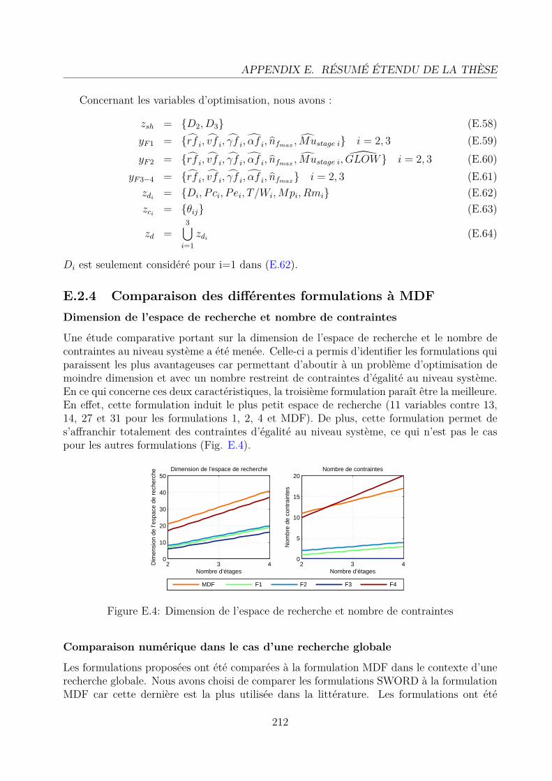
APPENDIX E. RÉSUMÉ ÉTENDU DE LA THÈSE
Concernant les variables d’optimisation, nous avons :
zsh = {D2, D3} (E.58)yF1 = {rf i, vf i, γf i, αf i, nfmax , Mustage i} i = 2, 3 (E.59)yF2 = {rf i, vf i, γf i, αf i, nfmax , Mustage i, GLOW} i = 2, 3 (E.60)
yF3−4 = {rf i, vf i, γf i, αf i, nfmax} i = 2, 3 (E.61)zdi = {Di, P ci, P ei, T/Wi,Mpi, Rmi} (E.62)zci = {θij} (E.63)
zd =3⋃i=1
zdi (E.64)
Di est seulement considéré pour i=1 dans (E.62).
E.2.4 Comparaison des différentes formulations à MDFDimension de l’espace de recherche et nombre de contraintes
Une étude comparative portant sur la dimension de l’espace de recherche et le nombre decontraintes au niveau système a été menée. Celle-ci a permis d’identifier les formulations quiparaissent les plus avantageuses car permettant d’aboutir à un problème d’optimisation demoindre dimension et avec un nombre restreint de contraintes d’égalité au niveau système.En ce qui concerne ces deux caractéristiques, la troisième formulation paraît être la meilleure.En effet, cette formulation induit le plus petit espace de recherche (11 variables contre 13,14, 27 et 31 pour les formulations 1, 2, 4 et MDF). De plus, cette formulation permet des’affranchir totalement des contraintes d’égalité au niveau système, ce qui n’est pas le caspour les autres formulations (Fig. E.4).
2 3 40
10
20
30
40
50Dimension de l’espace de recherche
Dim
ensi
on d
e l’e
spac
e de
rec
herc
he
Nombre d’étages2 3 4
0
5
10
15
20Nombre de contraintes
Nom
bre
de c
ontr
aint
es
Nombre d’étages
MDF F1 F2 F3 F4
Figure E.4: Dimension de l’espace de recherche et nombre de contraintes
Comparaison numérique dans le cas d’une recherche globale
Les formulations proposées ont été comparées à la formulation MDF dans le contexte d’unerecherche globale. Nous avons choisi de comparer les formulations SWORD à la formulationMDF car cette dernière est la plus utilisée dans la littérature. Les formulations ont été
212

E.2. FORMULATIONS MDO UTILISANT UNE DÉCOMPOSITION EN ÉTAGES
testées en utilisant le même algorithme d’optimisation, les mêmes initialisations et les mêmesréglages. L’algorithme d’optimisation sélectionné est l’algorithme génétique, car étant le plusrépandu dans la conception de lanceurs dans le cas de recherches globales. La populationinitiale est composée de 100 individus. Dix tests ont été effectués à partir d’initialisationsaléatoires afin de rendre la comparaison moins sensible à l’initialisation et à la part d’aléatoirede l’algorithme génétique. La comparaison entre les différentes formulations a été réaliséesuivant trois critères : le temps écoulé pour trouver un premier design faisable à partird’initialisation aléatoire, la capacité d’optimiser la fonction objectif et la qualité du meilleurpoint trouvé. La comparaison est effectuée en considérant un temps de calcul fixé (10 heures).
La figure E.5 indique les résultats moyens obtenus pour chacune des formulations. Lediagramme de gauche indique les meilleures solutions obtenues à l’arrêt de l’algorithme.Le diagramme central représente les temps de calcul moyens nécessaires pour trouver unpremier concept faisable à partir d’une initialisation aléatoire. Finalement, le diagrammede droite indique l’amélioration de la fonction objectif durant le processus d’optimisation.La figure E.6 représente les performances des différentes formulations concernant la qualitédu meilleur point obtenu et le temps nécessaire pour trouver un premier concept faisable.
MDF F1 F2 F3 F4140
145
150
155
160
GLO
W m
oyen
(t)
Moyenne des meilleurs points trouvés
MDF F1 F2 F3 F40
100
200
300
400
500
Dur
ée é
coul
ée m
oyen
ne (
min
)
Durées moyennes pour trouver un design faisable
MDF F1 F2 F3 F4−15
−10
−5
0
Am
élio
ratio
n m
oyen
ne (
%)
Amélioration moyenne de la fonction objectif
Figure E.5: Comparaison des méthodes dans le cas d’une recherche globale
La troisième formulation est celle qui aboutit auxmeilleurs résultats. En effet, cette formulation per-met d’obtenir la meilleure solution, est capable detrouver un premier design faisable dans le tempsle plus faible et conduit à la meilleure améliora-tion de la fonction objectif. Ceci est principalementdû à la gestion des couplages massiques qui est ef-fectuée au niveau sous-système, permettant d’éviterl’utilisation de contraintes d’égalité au niveau sys-tème et par conséquent permettant d’améliorer sig-nificativement l’efficacité de la recherche globale. Deplus, cette méthode induit la plus faible dimension del’espace de recherche au niveau système. Pour toutesces raisons, nous avons choisi cette méthode afin dedévelopper dans la prochaine section une stratégied’optimisation dédiée à la décomposition en étages.
0 100 200 300 400 500140
145
150
155
160GLOW vs durée écoulée pour trouver un design faisable
Durée écoulée pour trouver un design faisable (min)
GLO
W m
oyen
(t)
F3
F2
MDFF4
F1
Figure E.6: Synthèse des résultatsobtenus
213

APPENDIX E. RÉSUMÉ ÉTENDU DE LA THÈSE
E.2.5 ConclusionLa comparaison des méthodes a montré que l’utilisation d’une formulation SWORD ap-propriée permet d’améliorer significativement l’efficacité du processus d’optimisation parrapport à la méthode MDF, la plus utilisée dans la littérature. Néanmoins, même si cetteformulation associée à un algorithme génétique permet de trouver relativement rapidementun design faisable et de l’améliorer significativement, le processus d’optimisation ainsi forméprésente une vitesse de convergence relativement faible. De plus, cette formulation, incluantune phase d’optimisation au niveau sous système, peut poser des problèmes de temps decalcul lorsqu’elle est utilisée avec un algorithme génétique qui requiert par essence un grandnombre d’appels aux sous systèmes afin d’optimiser la fonction objectif. Pour ces raisons, ilapparaît essentiel de développer une stratégie d’optimisation afin d’exploiter les spécificitésde la décomposition en étages directement dans le processus d’optimisation. Ceci est l’objetde la prochaine section.
Remarque E.2.2. Au vu des résultats obtenus dans cette section, nous utiliserons la troisièmeformulation SWORD dans la section suivante afin d’établir la stratégie d’optimisation.
E.3 Stratégie d’optimisation dédiée à la décompositionen étages
E.3.1 Identification des besoinsLe choix de la stratégie d’optimisation est un point clé dans le processus de conception delanceurs. En effet, à la fois les recherches globales et locales sont requises afin d’explorerun large espace de recherche (bornes sur les variables d’optimisation) et de converger effi-cacement vers un optimum. Nous avons pris en compte les cinq exigences suivantes pourl’élaboration de la stratégie d’optimisation :
1. trouver rapidement des designs faisables (i.e. satisfaisant les contraintes de conceptionet de couplage), à partir d’initialisation aléatoire,
2. une fois le domaine de recherche faisable atteint, converger rapidement vers un opti-mum,
3. être robuste vis-à-vis de l’initialisation (stabilité des résultats),
4. converger sur des domaines de recherche très importants,
5. limiter au maximum l’intervention de l’utilisateur.
Afin de satisfaire toutes ces exigences, nous proposons une stratégie d’optimisation en 3phases. Dans la première phase, nous exploitons la décomposition en étages pour effectuerune exploration séquentielle des différentes variables du niveau système. Une fois des designsfaisables trouvés, une première étape d’optimisation (phase II) est effectuée en utilisantl’algorithme de Nelder & Mead (ou l’algorithme EGO si l’espace de recherche présente desoptima locaux), dans le but d’atteindre un point proche de l’optimum. Dans la seconde
214

E.3. STRATÉGIE D’OPTIMISATION DÉDIÉE À LA DÉCOMPOSITION EN ÉTAGES
étape de l’optimisation (phase III), nous effectuons une optimisation par un algorithme àbase de calculs de gradients pour converger rapidement vers l’optimum.Remarque E.3.1. Dans cette partie, nous ne décrivons que les algorithmes utilisés au niveausystème. En ce qui concerne le niveau sous-système, puisque les problèmes sont relativementfaciles à résoudre, nous utilisons un algorithme SQP (Sequential Quadratic Programming)standard dans toutes les phases du processus d’optimisation.
z1
z2design non faisabledesign faisable
(a) Phase I (a) : Exploration de l’espace derecherche
z1
z2design non faisabledesign faisable
(b) Phase I (b) : sélection des designs fais-ables
(c) Phase II : première optimisation (d) Phase III : seconde optimisation
Figure E.7: Stratégie d’optimisation
E.3.2 Description de la stratégie d’optimisationPhase I : exploration
La phase d’exploration consiste à utiliser la décomposition en étages afin de subdiviserl’ensemble des variables d’optimisation du niveau système (Fig. E.8) et de réduire l’exploration
215

APPENDIX E. RÉSUMÉ ÉTENDU DE LA THÈSE
globale à une suite d’explorations élémentaires. A cette fin, l’ensemble des variables d’optimisationdu niveau système est divisé en sous-ensembles élémentaires regroupant les variables inter-venant dans chacune des phases de vol. Par exemple, pour la configuration triétage dulanceur, les variables d’optimisation du niveau système peuvent être réparties en deux sous-ensembles zsh2 ∪ y12 et zsh3 ∪ y23 où :
zsh2 = {D2} (E.65)zsh3 = {D3} (E.66)y12 = {rf1 , vf1 , γf1 , αf1} (E.67)y23 = {rf2 , vf2 , γf2 , αf2 , nfmax} (E.68)
Le principe de l’exploration est le suivant :1. explorer le sous-ensemble composé des variables d’optimisation intervenant dans la
phase de vol du troisième étage (zsh3 et y23), et garder les valeurs pour lesquellesl’optimisation du troisième étage converge (z◦sh3 et y◦23),
2. étant données z◦sh3 , y◦23 et f ◦3 (masse optimisée du troisième étage), explorer le sous-
ensemble composé des variables d’optimisation intervenant dans les phases de vol despremier et second étages (zsh2 et y12) et garder les valeurs pour lesquelles les optimi-sations de ces étages convergent.
Ainsi, l’ensemble des variables faisables du niveau système est donné par :
z◦sh = z◦sh2 ∪ z◦sh3 (E.69)
y◦ = y◦12 ∪ y◦23 (E.70)
Cette méthode d’exploration permet de réduire le coût calculatoire par rapport à uneexploration aléatoire standard (exploration simultanée de toutes les variables du niveausystème), car l’exploration globale est réduite à une série d’explorations élémentaires et leprocessus mis en place assure la cohérence des configurations des étages entre les différentesphases d’exploration.
TEMPS
PHASE DE VOLETAGE 3
PHASE DE VOLETAGE 2
PHASE DE VOLETAGE1
VITESSE
y23
y12
zsh3
zsh2
Optimiseurétage 2
Optimiseur global
zsh2y
12 f 1
Optimiseurétage 1
f 2+
PHASE 1.2
Optimiseurétage 3
Optimiseur global
zsh3y
23 f 3
PHASE 1.1
Figure E.8: Stratégie d’exploration
216

E.3. STRATÉGIE D’OPTIMISATION DÉDIÉE À LA DÉCOMPOSITION EN ÉTAGES
Phase II : première étape de l’optimisation
A partir des points faisables trouvés lors de la phase d’exploration, une première phased’optimisation à partir d’algorithmes ne nécessitant pas de calculs de dérivées est réalisée.Pour ce faire, nous utilisons l’algorithme de Nelder & Mead [Nelder and Mead, 1965] oul’algorithme EGO [Jones, 2001] si l’espace de recherche est trop irrégulier (présence d’optimalocaux). Nous avons choisi d’utiliser en priorité l’algorithme de Nelder & Mead car celui-ci nenécessite pas de réglages particuliers de l’utilisateur. Cet algorithme requiert de trouver n+1points faisables, où n représente la dimension de l’espace de recherche au niveau système.Cette phase a pour but de trouver un point dans le voisinage de l’optimum. Ce point serautilisé comme initialisation pour l’algorithme utilisé dans la phase 3.
Phase III : seconde étape de l’optimisation
Puisque la formulation SWORD proposée comporte deuxniveaux d’optimisation, un algorithme de type gradient au niveausystème requiert des calculs de dérivées qui nécessitent autant deréoptimisations des sous-systèmes qu’il y a de variables de con-ception au niveau système (calcul par différences finies). Ceci in-duit un coût en calculs important et réduit fortement l’efficacitédu processus d’optimisation. Une solution possible pour sur-monter cette difficulté consiste à utiliser l’analyse post-optimale(POA pour Post-Optimality Analysis) afin d’estimer le gradientde la fonction objectif à partir des informations de convergencedonnées par le niveau sous-système. Puisque les optimisationsdes différents sous-systèmes sont effectuées de manière séquen-tielle, nous utilisons l’équation de sensibilité globale (GSE pour
Etage 3
Etage 2
Etage 1
y3
y3
y2
Optimiseur global
zsh,y23
zsh, y12,y23
zsh,y12
f
Figure E.9: Processusd’optimisation enphase 3
Global Sensitivity Equation) au niveau système. L’analyse post-optimale permet d’estimer legradient de la fonction objectif au niveau système f à partir des multiplicateurs de Lagrangeassociés aux conditions de Karush-Kuhn-Tucker des différents sous-systèmes [Sobieszczanski-Sobieski, 1990; Braun et al., 1993]. Au moyen de ces deux techniques d’optimisation, legradient de la fonction objectif du niveau système est estimé sans avoir recours à des réop-timisations de sous-systèmes (Eq. E.71).
dy3dzshdy3
dy23dy3
dy12dy2
dzshdy2
dy23dy2
dy12df
dzshdf
dy23df
dy12
=
1 0 0 0 0 0 0 0 00 1 0 0 0 0 0 0 00 0 1 0 0 0 0 0 0
− ∂y2∂y3
− λT2
∂e2∂y3
0 0 1 0 0 0 0 0
0 − ∂y2∂y3
− λT2
∂e2∂y3
0 0 1 0 0 0 0
0 0 − ∂y2∂y3
− λT2
∂e2∂y3
0 0 1 0 0 0
− ∂f∂y3
− λT1
∂e1∂y3
0 0 − ∂f∂y2
− λT1
∂e1∂y2
0 0 1 0 0
0 − ∂f∂y3
− λT1
∂e1∂y3
0 0 − ∂f∂y2
− λT1
∂e1∂y2
0 0 1 0
0 0 − ∂f∂y3
− λT1
∂e1∂y3
0 0 − ∂f∂y2
− λT1
∂e1∂y2
0 0 1
−1
.
∂y3∂zsh
+ λ3∂e3
∂zzh∂y3
∂y23+ λ3
∂e3∂y23
∂y3∂y12
+ λ3∂e3
∂y12∂y2
∂zsh+ λ2
∂e2∂zzh
∂y2∂y23
+ λ2∂e2
∂y23∂y2
∂y12+ λ2
∂e2∂y12
∂f∂zsh
+ λ1∂e1
∂zzh∂f
∂y23+ λ1
∂e1∂y23
∂f∂y12
+ λ1∂e1
∂y12
(E.71)
où λi sont les multiplicateurs de Lagrange associés au ième étage et ei regroupent lescontraintes d’égalité et celles d’inégalité saturées.
217

APPENDIX E. RÉSUMÉ ÉTENDU DE LA THÈSE
E.3.3 Analyse des performances de la stratégie d’optimisation
Afin d’évaluer les performances et la robustesse du processus d’optimisation, nous avonschoisi d’effectuer 10 optimisations différentes, à partir de 10 recherches de points faisablesréalisées par la phase I. Les domaines de recherche des variables du niveau système ont étéchoisis très importants de manière à estimer l’efficacité de la méthode sans connaissance apriori de l’utilisateur (exigence n◦ 3). A partir des designs faisables trouvés, nous avonsréalisé 10 premières optimisations à l’aide de l’algorithme de Nelder & Mead puis nous avonsachevé l’optimisation par l’algorithme basé sur des calculs de gradients.
(a) Evolution de la fonction objectif pendant la phaseIII
(b) Synthèse des 10 cas
Figure E.10: Comportement du processus d’optimisation
Dans tous les cas, le processus d’optimisation converge avec une différence relative max-imale de 0.2% par rapport à l’optimum de référence (qui est obtenu en restreignant lesdomaines de recherche et en réglant finement les optimiseurs, ce qui nécessite une forte in-tervention de l’utilisateur et requiert beaucoup de temps). En effet, l’écart relatif entre ledesign obtenu et l’optimum de référence est réduit en moyenne de 96% (Fig. E.10). La duréetotale moyenne du processus d’optimisation est de 4 heures (MATLAB, 2.4 GHz Dual CorePentium / Windows XP). Afin de quantifier la robustesse de l’algorithme d’optimisation,définie ici comme la capacité à converger sur un espace de recherche très important, nousavons comparé la dispersion des 10 designs obtenus à celle des initialisations (faisables) trou-vées après la première phase (Tab. E.11 et Fig. E.12). Les résultats montrent que la stratégied’optimisation proposée est robuste car la dispersion des optima trouvés est seulement 4.44%de celle des initialisations.
218
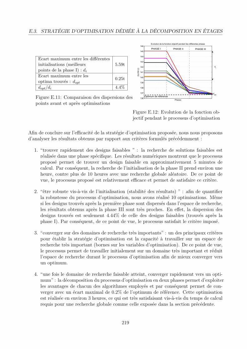
E.3. STRATÉGIE D’OPTIMISATION DÉDIÉE À LA DÉCOMPOSITION EN ÉTAGES
Ecart maximum entre les différentes5.59tinitialisations (meilleurs
points de la phase I) : diEcart maximum entre les 0.25toptima trouvés : doptdopt/di 4.4%
Figure E.11: Comparaison des dispersions despoints avant et après optimisations
Figure E.12: Evolution de la fonction ob-jectif pendant le processus d’optimisation
Afin de conclure sur l’efficacité de la stratégie d’optimisation proposée, nous nous proposonsd’analyser les résultats obtenus par rapport aux critères formulés précédemment :
1. “trouver rapidement des designs faisables ” : la recherche de solutions faisables estréalisée dans une phase spécifique. Les résultats numériques montrent que le processusproposé permet de trouver un design faisable en approximativement 5 minutes decalcul. Par conséquent, la recherche de l’initialisation de la phase II prend environ uneheure, contre plus de 10 heures avec une recherche globale aléatoire. De ce point devue, le processus proposé est relativement efficace et permet de satisfaire ce critère.
2. “être robuste vis-à-vis de l’initialisation (stabilité des résultats) ” : afin de quantifierla robustesse du processus d’optimisation, nous avons réalisé 10 optimisations. Mêmesi les designs trouvés après la première phase sont dispersés dans l’espace de recherche,les résultats obtenus après la phase III sont très proches. En effet, la dispersion desdesigns trouvés est seulement 4.44% de celle des designs faisables (trouvés après laphase I). Par conséquent, de ce point de vue, le processus satisfait le critère imposé.
3. “converger sur des domaines de recherche très importants” : un des principaux critèrespour établir la stratégie d’optimisation est la capacité à travailler sur un espace derecherche très important (bornes sur les variables d’optimisation). De ce point de vue,le processus permet de travailler initialement sur un domaine très important et réduitl’espace de recherche durant le processus d’optimisation afin de mieux converger versun optimum.
4. “une fois le domaine de recherche faisable atteint, converger rapidement vers un opti-mum” : la décomposition du processus d’optimisation en deux phases permet d’exploiterles avantages de chacun des algorithmes employés et par conséquent permet de con-verger avec un écart maximal de 0.2% de l’optimum de référence. Cette optimisationest réalisée en environ 3 heures, ce qui est très satisfaisant vis-à-vis du temps de calculrequis pour une recherche globale comme celle exposée dans la section précédente.
219

APPENDIX E. RÉSUMÉ ÉTENDU DE LA THÈSE
Conclusion
Cette thèse est centrée sur le développement de méthodes MDO consacrée aux études d’avantprojet de conception de lanceurs. Notre contribution porte sur le développement de nou-velles formulations MDO, appelées SWORD (Stage-Wise decomposition for Optimal RocketDesign), exploitant une décomposition transversale du processus de conception selon lesdifférentes phases de vol du lanceur. Les formulations SWORD permettent de répartir lacomplexité du problème entre les niveaux système et sous-système et de transformer le prob-lème global d’optimisation en la coordination d’une série de sous-problèmes qui peuvent êtrerésolus plus rapidement.
D’après l’étude bibliographique portant sur l’application des méthodes MDO existantes àla conception lanceurs, nous avons proposé une nouvelle formulation du problème de concep-tion de lanceurs centrée sur l’optimisation de trajectoire et inspirée de l’architecture physiquedes lanceurs. A cette fin, nous avons développé quatre formulations MDO et les avons com-parées à la méthode MDF dans le cas d’une recherche globale. Les résultats de cette étude ontmontré que deux des formulations proposées (seconde et troisième) se détachent des autreset permettent d’améliorer l’efficacité du processus d’optimisation par rapport à la méthodeMDO la plus utilisée dans la conception de lanceurs (MDF), en termes de temps de calculpour trouver un design faisable à partir d’initialisation aléatoire et de qualité de la solutiontrouvée pour un temps de calcul donné. Par conséquent, avec la formulation appropriée, ladécomposition en étage permet de rendre plus efficace l’utilisation d’algorithmes de rechercheglobale pour résoudre le problème de conception de lanceurs à partir d’initialisation aléatoireet sans requérir de connaissances spécifiques sur le domaine de variation des variables de con-ception. Néanmoins, cette étude a montré que l’utilisation de la recherche globale seule n’estpas suffisante pour obtenir un optimum en un temps de calcul acceptable (quelques heures).Par conséquent, le développement d’une stratégie d’optimisation spécifique est nécessaire.
Dans la seconde partie de cette thèse, nous avons proposé une stratégie d’optimisationdédiée aux formulations SWORD. A cette fin, nous avons utilisé la troisième formulationSWORD pour proposer une stratégie d’optimisation ayant pour but de rapidement trou-ver un point faisable, de converger vers un optimum en un temps de calcul limité, deréaliser l’optimisation sur des domaines de recherche très importants (bornes sur les variablesd’optimisation) et d’améliorer la robustesse du processus vis-à-vis de l’initialisation. Afin desatisfaire ces exigences, nous avons proposé une optimisation en trois phases.
La première phase s’inspire de la troisième formulation SWORD et consiste à explorerséquentiellement les différents ensembles de variables du niveau système intervenant dansles différentes phases de vol. Cette méthode permet de réduire considérablement le tempsde calcul pour trouver un design faisable par rapport à une recherche aléatoire globale.
A partir des designs faisables trouvés pendant la première phase, nous avons choisid’effectuer l’optimisation en deux étapes. La première étape consiste en une optimisationsans calcul de gradient, utilisant l’algorithme de Nelder & Mead (ou l’algorithme EfficientGlobal Optimization si le problème présente beaucoup de minima locaux), dans le but derapidement atteindre le voisinage d’un optimum. Finalement, à partir du meilleur designtrouvé lors de la première étape d’optimisation, la seconde étape consiste à réaliser une
220

E.3. STRATÉGIE D’OPTIMISATION DÉDIÉE À LA DÉCOMPOSITION EN ÉTAGES
optimisation à base de calculs de gradients, sur un espace de recherche limité autour del’optimum. Afin de réduire le temps de calcul de cette phase, nous avons remplacé le calculclassique par différences finies du gradient de la fonction objectif du niveau système parune estimation exploitant les informations de convergence des sous-systèmes (Analyse PostOptimale et Equation de Sensibilité Globale).
Une analyse globale du processus complet (formulation MDO et stratégie d’optimisation)a ensuite été menée afin d’évaluer les performances de la méthode SWORD. Les résultatsmontrent que le processus d’optimisation permet d’atteindre l’optimum de référence à 0,2%près, en un temps de calcul inférieur à quatre heures, ce qui est satisfaisant pour les phasesde conception avant projet, par comparaison avec les approches classiques qui prennent plusde dix heures de calculs lorsqu’elles prennent en compte un espace de recherche aussi impor-tant. Cette analyse a validé la stratégie d’optimisation proposée et a montré que l’utilisationde la décomposition en étages est utile afin de résoudre en temps de calcul limité le problèmeMDO de conception de lanceur sans requérir de connaissances a priori de l’utilisateur.
Afin d’améliorer la méthode MDO proposée, plusieurs extensions des travaux peuventêtre proposées. Le processus de conception décrit est actuellement dédié aux phases d’avantprojet dans lesquelles des modèles simplifiés sont utilisés. Il serait utile de tester la méthodeMDO proposée avec des modèles disciplinaires plus détaillés, incluant davantage de cou-plages entre les disciplines.
De plus, dans cette thèse, nous avons comparé les méthodes SWORD avec la méthodeMDF mais pas avec les autres méthodes MDO telles BLISS, ATC, CSSO, etc. La compara-ison des méthodes SWORD avec ces méthodes serait très intéressante mais requerrait aupréalable d’élaborer des modèles disciplinaires plus complexes afin de pouvoir appliquer lesméthodes MDO présentes dans la littérature.
D’autre part, comme la méthode SWORD est principalement consacrée aux phasesd’avant projet dans lesquelles des modèles simplifiés sont utilisés, il serait utile d’incorporerla gestion d’incertitudes à la méthode actuelle afin d’assurer la cohérence de la configurationtrouvée dans les phases ultérieures du processus de conception.
Par ailleurs, la méthode de commande optimale développée dans cette thèse est unecommande directe. Il serait intéressant d’étudier dans de futurs travaux d’autres méthodesd’optimisation de trajectoire (e.g. commande indirecte) afin de choisir laquelle est la plusadaptée au problème posé.
En outre, la méthode SWORD a été testée sur un problème de conception classique delanceurs consommables avec étagement séquentiel (pas de boosters). Il serait intéressantde transposer et tester les formulations SWORD à des problèmes plus complexes commeles lanceurs avec étagement parallèle ou les lanceurs réutilisables. De la même manière, leprocessus actuel gère seulement les variables continues. L’introduction de variables discrètesserait profitable afin de considérer dans le processus de conception d’autres caractéristiquesdu lanceur telles le type de propulsion, le nombre d’étages, etc.
Enfin, dans cette thèse, nous avons appliqué la méthode SWORD à des problèmes monoobjectif. Il serait très intéressant de tester notre méthode dans le cas de problèmes multiobjectif (e.g. la maximisation de la charge utile et la minimisation du coût). Ce cas d’étudenous permettrait de concevoir une famille de lanceurs et d’être capable de proposer plusieurschoix de lanceurs possibles pour différentes missions.
221


Appendix F
Publications and communications
Publications in international journalsM. Balesdent, N. Bérend, Ph. Dépincé and A. Chriette. A Survey of MutidisciplinaryDesign Optimization methods in Launch Vehicle Design, Structural and MultidisciplinaryOptimization, Springer. DOI:10.1007/s00158-011-0701-4. accepted, pending publication
M. Balesdent, N. Bérend and Ph. Dépincé. Multidisciplinary Design Optimization of amulti-stage launch vehicle using flight phases decomposition, International Journal for Sim-ulation and Multidisciplinary Design Optimization, EDP Sciences. accepted, pending pub-lication
M. Balesdent, N. Bérend and Ph. Dépincé. Optimal Design of Expendable Launch Vehiclesusing Stage-Wise Multidisciplinary Design Optimization Formulation, Journal of Spacecraftand Rockets, AIAA. accepted, pending publication
Communications in international conferencesM. Balesdent, N. Bérend and Ph. Dépincé. New MDO approaches for Launch Vehicle De-sign, 4th European Conference for Aerospace Sciences, July 4 – 8 2011, St Petersburg, Russia.
M. Balesdent, N. Bérend and Ph. Dépincé. MDO formulations and techniques adapted tomulti-stage launch vehicle design, 9th ISSMO World Congress on Structural and Multidisci-plinary Optimization. June 13 – 17 2011, Shizuoka, Japan
M. Balesdent, N. Bérend and Ph. Dépincé. Optimal Design of Expendable Launch Ve-hicles using Stage-Wise MDO Formulation, 13th AIAA/ISSMO Multidisciplinary AnalysisOptimization Conference. September 13 – 15 2010, Fort Worth, USA. Finalist of the “BestStudent Paper Competition”
M. Balesdent, N. Bérend and Ph. Dépincé. Multidisciplinary Design Optimization ofa multi-stage launch vehicle using flight phases decomposition, 3rd ASMDO InternationalConference on Multidisciplinary Design Optimization and Applications. June 21 – 23 2010,Paris, France
223

Bibliography
Agte, J. (2005). A Tool for Application of Bi-Level Integrated System Synthesis to Multi-disciplinary Design Optimization Problems. In DGLR-2005-241, German Air and SpaceCongress, Friedrichshafen, Germany.
Agte, J., de Weck, O., Sobieszczanski-Sobieski, J., Arendsen, P., Morris, A., and Spieck, M.(2009). MDO : assessment and direction for advancement - an opinion of one internationalgroup. Structural Multidisciplinary Optimization, DOI10.1007/s00158-009-0381-5.
Akhtar, S. and Linshu, H. (2005a). Simulation-based Optimization strategy for liquid fu-eled multi-stage space launch vehicle. In 6th International Conference on Parallel andDistributed Computing, Applications and Technologies (PDCAT’05). Dalian, China.
Akhtar, S. and Linshu, H. (2005b). Support vector machine based trajectory metamodel forconceptual design of multi-stage space launch vehicle. In Computational Intelligence andSecurity, vol 3801:528-535. Springer Berlin / Heidelberg.
Akhtar, S. and Linshu, H. (2006). Support Vector Regression-driven Multidisciplinary DesignOptimization for multi-stage launch vehicle considering throttling effect. In 44th AIAAAerospace Sciences Meeting and Exhibit. Reno, Nevada, USA.
Alexandrov, N. and Hussaini, M. (1995). Multidisciplinary Design Optimization : Stateof the Art. Proceedings of the ICASE / NASA Langley Workshop on MultidisciplinaryDesign Optimization, SIAM Proccedings Series.
Alexandrov, N. and Lewis, R. (2000). Algorithmic Perspectives on Problem Formulations inMDO. In 8th AIAA/UASAF/NASA/ISSMO Symposium on Multidisciplinary Analysis &Optimization. Long Beach, CA, USA.
Allison, J. (2004). Complex system Optimization : a Comparison of Analytical TargetCascading, Collaborative Optimization and other formulations. Master’s thesis, Universityof Michigan, USA.
Allison, J., Kokkolaras, M., Zawislak, M., and Papalambros, P. (2005). On the Use ofAnalytical Target Cascading and Collaborative Optimization for Complex System Design.In 6th World Congress on Structural and Multidisciplinary Optimization. 30 May-03 June,Rio de Janeiro, Brazil.
225

BIBLIOGRAPHY
Altus, T. (2002). A Response Surface Methodology for Bi-Level Integrated System Synthesis(BLISS). NASA Technical Report n◦ NASA/CR-2002-211652. NASA Langley ResearchCenter, USA.
Alyaqout, S., Papalambros, P., and Ulsoy, A. (2005). Quantification and use of systemcoupling in decomposed design optimization problems. In ASME International MechanicalEngineering Congress and Exposition. Orlando, FL, USA.
Amouroux, F. (2008). Présentation des logiciels PERSEUS. CNES Technical Report - PER-NT-3100000-4.
Armijo, L. (1966). Minimization of functions having Lipschitz continuous first partial deriva-tives. Pacific Journal of Mathematics, vol 16:1-3.
Auroux, D., Clément, J., Hermetz, J., Masmoudi, M., and Parte, Y. (2009). Etat de l’artet nouvelles tendances en conception collaborative. Optimisation multidisciplinaire en mé-canique. Hermes Science Publishing, ISTE Wiley. London, UK.
Bäck, T. (1996). Evolutionary Algorithms in Theory and Practice. Oxford University Press.UK.
Bäck, T., Fogel, D., and Michalewicz, Z. (1997). Handbook of Evolutionary Computation.Oxford University Press.
Bairstow, B., de Weck, O., and Sobieszczanski-Sobieski, J. (2006). Multiobjec-tive Optimization of Two-Stage Tockets for Earth-To-Orbit Launch. In 47thAIAA/ASME/ASCE/AHS/ASC Structures, structural Dynamics and Materials Confer-ence. Newport, RI, USA.
Balesdent, M., Bérend, N., and Dépincé, P. (2010a). Optimal Design of Expendable LauchVehicles using Stage-wise MDO formulation. In 13th AIAA/ISSMO MultidisciplinaryAnalysis and Optimization conference. Fort Worth, Texas, USA.
Balesdent, M., Bérend, N., and Dépincé, P. (2011a). MDO Formulations and Techniquesadapted to Multi-stage Launch Vehicle Design. In 9th World Congress on Structural andMultidisciplinary Optimization, Shizuoka, Japan.
Balesdent, M., Bérend, N., and Dépincé, P. (2011b). New MDO Approaches for Launch Ve-hicle Design. In 4th European Conference for AeroSpace Sciences, St. Petersburg, Russia.
Balesdent, M., Bérend, N., and Dépincé, P. (2011c). Optimal Design of Expendable LauchVehicles using Stage-wise MDO formulation. Journal of Spacecraft and Rockets, AIAA.publication pending.
Balesdent, M., Bérend, N., Dépincé, P., and Chriette, A. (2010b). Multidisciplinary DesignOptimization of a multi-stage launch vehicle using flight phases decomposition. In 3rd In-ternational Conference on Multidisciplinary Design Optimization and applications. Paris,France.
226

BIBLIOGRAPHY
Balesdent, M., Bérend, N., Dépincé, P., and Chriette, A. (2011d). A Survey of Multi-disciplinary Design Optimization Techniques in Launch Vehicle Design. Structural andMultidisciplinary Optimization, Springer. publication pending.
Balesdent, M., Bérend, N., Dépincé, P., and Chriette, A. (2011e). Multidisciplinary DesignOptimization of a multi-stage launch vehicle using flight phases decomposition. In Interna-tional Journal for Simulation and Multidisciplinary Design Optimization, EDP Sciences.publication pending.
Balling, R. and Sobieszczanski-Sobieski, J. (1994). Optimization of coupled systems : acritical overview of approaches. NASA / ICASE Report n◦ 94-100.
Balling, R. and Wilkinson, C. (1997). Execution of Multidisciplinary Design Optimizationapproaches on common test problems. AIAA Journal vol 35(1):178-186.
Banach, S. (1922). Sur les opérations dans les ensembles abstraits et leur application auxéquations intégrales. Fundamenta Mathematicae, vol 3:133-181.
Bayley, D. and Hartfield, R. (2007). Design Optimization of Space Launch Vehicles forMinimum Cost Using a Genetic Algorithm. In 43rd AIAA/ASME/SAE/ASEE JointPropulsion Conference and Exhibit. Cincinnati, OH, USA.
Bayley, D., Hartfield, R., Burkhalter, J., and Jenkins, R. (2008). Design Optimization of aSpace Launch Vehicle Using a Genetic Algorithm. Journal of Spacecraft and Rockets, vol45(4):733-740.
Bellman, R. (1957). Dynamic Programming. Princeton University Press. Princeton NJ.
Beltracchi, T. (1992). Decomposition Approach to Solving the All-Up Trajectory Optimiza-tion Problem. Journal of Guidance, Control, and Dynamics, vol 15(3):707-716.
Bérend, N. and Talbot, C. (1996). Overview of some optimal control methods adapted toexpendable and reusable launch vehicle trajectories. Aerospace Science and Technology,vol 10:222-232.
Bertsekas, D. (2005). Dynamic Programming and Optimal Control, 3rd Edition. Vol 1 & 2.Athena Scientific.
Betts, J. (1998). Survey of Numerical Methods for Trajectory Optimization. Journal ofGuidance, Control, and Dynamics, vol 21(2):193-207.
Boman, E. (1999). Infeasibility and negative curvature in optimization. PhD thesis, StanfordUniversity, USA.
Bonnans, J., Gilbert, J., Lemaréchal, C., and Sagastizábal, C. (2006). Numerical Optimiza-tion. Theoretical and Practical Aspects. Second Edition. Springer.
Brauer, G., Cornick, D., and Stevenson, R. (1977). Capabilities and Applications of theProgram to Optimize Simulated Trajectories (POST). NASA Contractor Report - 2770.
227

BIBLIOGRAPHY
Braun, R. (1996). Collaborative Optimization : An architecture for Large-Scale DistributedDesign. PhD thesis, Stanford University, USA.
Braun, R. and Kroo, I. (1995). Development and application of the Collaborative Opti-mization architecture in a multidisciplinary design environment. Multidisciplinary DesignOptimization : State of the Art, SIAM:98-116.
Braun, R., Kroo, I., and Gage, P. (1993). Post-Optimality Analysis In Aerospace VehicleDesign. In AIAA Aircraft Design, Systems and Operations Meeting. Monterey, CA, USA.
Braun, R., Kroo, I., Lepsch, R., Powell, R., and Stanley, D. (1995). Comparison of twomultidisciplinary optimization strategies for launch vehicle design. Journal of Spacecraftand Rockets, vol 32(3):404-410.
Braun, R., Moore, A., and Kroo, I. (1996). Use of the Collaborative Optimization Archi-tecture for Launch Vehicle Design. In 6th AIAA/USAF/NASA/ISSMO Symposium onMultidisciplinary Analysis and Optimization. Bellevue, WA, USA.
Briggs, G., Ray, T., and Milthorpe, J. (2007a). Evolutionay Algorithm use in Optimisationof a Launch Vehicle Stack Model. In 45th AIAA Aerospace Sciences Meeting and Exhibit.Reno, Nevada, USA.
Briggs, G., Ray, T., and Milthorpe, J. (2007b). Optimal design of an Australian mediumlaunch vehicle. Innovations in Systems and Software Engineering, vol 2(3):105-116.
Brown, N. and Olds, J. (2005). Evaluation of Multidisciplinary Optimization (MDO) tech-niques applied to a reusable launch vehicle. In 43rd AIAA Aerospace Sciences Meetingand Exhibit. Reno, Nevada, USA.
Brown, N. and Olds, R. (2006). Evaluation of Multidisciplinary Optimization TechniquesApplied to a Reusable Launch Vehicle. Journal of Spacecraft and Rockets, 43:1289-1300.
Bryson, A. (1999). Dynamic Optimization. Addison-Wesley Longman, Inc. Menlo-Park,California, USA.
Bryson, A. and Y-C., H. (1975). Applied Optimal Control : Optimization, Estimation andControl, Revised Printing. Taylor & Francis Inc. Levittown, USA.
Castellini, F. and Lavagna, M. (2009). Comparative analysis of multi-objective global op-timization techniques for launchers design. In 8th World Congress on Structural andMultidisciplinary Optimization. Lisbon, Portugal.
Castellini, F., Lavagna, M., and Erf, S. (2008). Concurrent optimization of launcher archi-tectures and ascent trajectories with global optimization algorithms. In 59th InternationalAstronautical Congress (IAC). Glasgow, Scotland.
Castellini, F., Lavagna, M., Riccardi, A., and Büskens, C. (2010). Multidisciplinary DesignOptimization Models and Algorithms for Space Launch Vehicles. In 13th AIAA/ISSMOMultidisciplinary Analysis Optimization Conference. Fort-Worth, TX. USA.
228

BIBLIOGRAPHY
Castellini, F., Riccardi, A., Lavagna, F., and Büskens, C. (2011). Global and Local Multi-disciplinary Optimization of Expendable Launch Vehicles. In 7th AIAA MultidisciplinaryDesign c Specialist Conference. Denver, CO. USA.
Chachuat, B. (2006). Non Linear and Dynamic Optimization, from Theory to Practice.Ecole Polytechnique de Lausanne, IC-32 : Winter Semester 2006/2007.
Chandila, P., Perez, V., and Renaud, J. (2004). Post-Optimality Analysis for Multidisci-plinary Systems using a Cumulative Response Surface Approximation. In 42nd AIAAAerospace Sciences Meeting and Exhibit. Reno, Nv, USA.
Chelouah, R. and Siarry, P. (2003). Genetic and Nelder-Mead algorithms hybridized for amore accurate global optimization of continuous multiminima functions. European Journalof Operational Research, vol 148:335-348.
Chittick, I. and Martins, J. (2008). Aero-structural optimization using adjoint coupled post-optimality sensitivities. Structural and Multidisciplinary Optimization, vol36:59-70.
Clement, J. (2009). Optimisation multi-disciplinaire : étude théorique et application à laconception des avions en phase d’avant projet. Institut Supérieur de l’Aéronautique et del’Espace. Toulouse, France.
Coello, C. (2002). Theoretical and numerical constraint-handling techniques used with evo-lutionary algorithms : a survey of the state of the art. Computer Methods in AppliedMechanics and Engineering, vol 191(11):1245-1287.
Collange, G., Delattre, N., Lemaire, F., and Quinquis, I. (2009). Different approaches tomultidisciplinary optimization for preliminary design of expendable launch vehicles. In3rd European Conference for Aerospace Sciences. Versailles, France.
Collange, G., Reynaud, S., and Hansen, N. (2010). Covariance matrix adaptation evolu-tion strategy for multidisciplinary optimization of expendable launcher family. In 13thAIAA/ISSMO Multidisciplinary Analysis Optimization Conference. Fort-Worth, TX.
Cormier, T., Scott, A., Ledsinger, L., McCormick, D., Way, D., and Olds, R. (2000). Com-parison of Collaborative Optimization to Conventional Design techniques for a ConceptualRLV. In 8th AIAA/USAF/NASA/ISSMO Symposium on Multidisciplinary Analysis andOptimization. Long Beauch, CA, USA.
Cramer, E., Dennis, J., Frank, P., Lewis, R., and Shubin, G. (1994). Problem Formulationfor Multidisciplinary Optimization. SIAM Journal of Optimization 4:754-776.
Deb, K. (1995). Optimization for engineering design: Algorithms and examples. Prentice-Hall.
Deb, K. (2000). An Efficient Constraint Handling Method for Genetic Algorithms. ComputerMethods in Applied Mechanics and Engineering, vol 186(2-4):311-338.
De Biasi, J.-M. (2002). Dossier de Définition du logiciel OPTAX 6.0.0. Technical RepostCNES-SEGIME, SEG/MU/02-102.
229

BIBLIOGRAPHY
De Boor, C. (1978). A Practical Guide to Splines. Springer-Verlag, New-York.
Delattre, N. and Mongrard, O. (2007). The Use of Multidisciplinary Optimization for theDesign of Expendable Launchers. In 2nd European Conference for AeroSpace Sciences(EUCASS). Brussels, Belgium.
DeMiguel, A. (2001). Two decomposition algorithms for nonconvex optimization problemswith global variables. PhD thesis, Stanford University, USA.
DeMiguel, V. and Murray, W. (2000). An Analysis of Collaborative Optimization Meth-ods. In 8th AIAA/USAF/NASA/ISSMO Symposium on Multidisciplinary Analysis andOptimization. Long Beach, CA, USA.
DeMiguel, V. and Murray, W. (2006). A local convergence analysis of bilevel decompositionalgorithms. Optimization Engineering vol7:99-133.
Dormand, J. and Prince, P. (1980). A family of embedded Runge-Kutta formulae. Journalof Computational and Applied Mathematics, vol6:19-26.
Du, X. and Chen, W. (2002). Efficient uncertainty analysis methods for multidisciplinaryrobust design. AIAA Journal vol 40(3):545-552.
Durand, N. and Alliot, J.-M. (1999). A Combined Nelder-Mead simplex and genetic algo-rithm. In Genetic and Evolutionary Computation Conference. Orlando, Fl, USA.
Duranté, N., Dufour, A., and Pain, V. (2004). Multidisciplinary Analysis and OptimisationApproach for the Design of Expendable Launchers. In 10th AIAA/ISSMO Multidisci-plinary Analysis and Optimization Conference. Albany, New-York, USA.
Duranté, N., Dufour, A., Ponçon, M., and Paulat, J. (2005). Integrated MultidisciplinaryOptimisation of Expendable Launcher Design. In 1st European Conference for AerospaceSciences. Moscow, Russia.
Eiben, A., Hinterding, R., and Michalewicz, Z. (1999). Parameter Control in EvolutionaryAlgorithms. IEEE Transactions on Evolutionary Algorithms, vol 3(2):124-141.
Erb, S. (2007). Development of Post-Optimality Analysis Algorithm for Optimal ControlProblems. PhD thesis, University of Stuttgart.
European Space Agency (2004). ESA Launch Vehicle Catalogue, Revision 15.
Filatyev, A. and Golikov, A. (2008). The complex Approach to Optimization of STS pa-rameters on the Maximum Principle basis. In 59th International Astronautical Congress(IAC). Glasgow, Scotland.
Filatyev, A., Golikov, A., Shanygin, A., and Voityshen, V. (2009). The local distributed crite-ria method for multidisciplinary optimization of launchers parameters. Acta Astronautica65:584-590.
230

BIBLIOGRAPHY
Fletcher, R. (1987). Practical Methods of Optimization, 2nd edition. John Wiley & Sons,Ltd.
Fraser-Andrews, G. (1999). A Multiple-Shooting Technique for Optimal Control. Journal ofOptimization theory and Applications, vol 102(2):299-313.
Gang, C., ans W. Zi-ming, X. M., and Si-Lu, C. (2005). Multidisciplinary Design Optimiza-tion of RLV Reentry Trajectory. In 13th AIAA/CIRA International Space Planes andHypersonic Systems and Technologies. Capua, Italy.
Gath, P. and Well, K. (2001). Trajectory Optimization Using A Combination of Direct Mul-tiple Shooting and Collocation. In AIAA Guidance, Navigation, and Control Conferenceand Exhibit. Montreal, Canada. AIAA 2001-4047.
Geethaikrishnan, C., Mujumbar, P., Sudhakar, K., and Adimurthy, V. (2008). GeneticAlgorithm Guided Gradient Search for Launch Vehicle Trajectory Optimization. In Inter-national Conference on Aerospace Science and Technology. Bangalore, India.
Geethaikrishnan, C., Mujumdar, P., Sudhakar, K., and Adimurthy, V. (2009). A Robust andEfficient Hybrid Algorithm for Global Optimization. In 2009 IEEE International AdvanceComputing Conference (IACC 2009). Pariala, India.
Gill, P., Murray, W., and Saunders, M. (1994). Large-scale SQP Methods and their applica-tion in Trajectory Optimization. Birkhäuser Verlag.
Gill, P., Murray, W., Saunders, M., and Wright, M. (1986). Users Guide for NPSOL (Ver-sion 4.0) : A Fortran Package for Nonlinear Programming. Technical Report SOL 86-2.Stanford University, USA.
Gill, P., Murray, W., and Wright, M. (1981). Practical Optimization. Academic Press,New-York, USA.
Goldberg, D. (1989). Genetic Algorithms in Search, Optimization and Machine Learning.Addison-Wesley Professional.
Han, J. and Papalambros, P. (2010). A Note on the Convergence of Analytical TargetCascading With Infinite Norms. Journal of Mechanical Design, vol132/034502.
Hargraves, C. and Paris, S. (1987). Direct Trajectory Optimization Using Nonlinear Pro-gramming and Collocation. Journal of Guidance, Control and Dynamics vol 10(4):338-342.
Holland, J. (1975). Adaptation in natural and artificial systems. Ann Arbor : the Universityof Michigan Press. USA.
Huang, C. and Bloebaum, C. (2004). Multi-Objective Pareto Concurrent SubSpace Opti-mization for Multidisciplinary Design. In 42nd AIAA Aerospace Sciences Meeting andExhibit. Reno, Nevada, USA.
231

BIBLIOGRAPHY
Humble, R., Henry, G., and Larson, W. (1995). Space Propulsion Analysis and Design.Mc-Graw Hill.
Jodei, J., Ebrahimi, M., and Roshanian, J. (2006). An Automated Approach to Multidis-ciplinary System Design Optimization of Small Solid Propellant Launch Vehicles. In 1stISSCAA International Symposium on Systems and Control in Aerospace and Astronautics.Harbin, China.
Jodei, J., Ebrahimi, M., and Roshanian, J. (2009). Multidisciplinary design optimizationof a small solid propellant launch vehicle using system sensitivity analysis. StructuralMultidisciplinary Optimization vol 38:93-100.
Jones, D. (2001). A taxonomy of global optimization methods based on response surfaces.Journal of Global Optimization, vol 21:345-383.
Jones, D., Schonlau, M., and Welch, W. (1998). Efficient Global Optimization of ExpensiveBlack-Box Functions. Journal of Global Optimization, vol 13:455-492.
Kalden, O. (2007). Multidisciplinary Design and Trajectory Optimization of the ReusableLaunch Vehicle Concept Hopper. In 3rd International Conference on Recent Advances inSpace Technologies. Istanbul, Turkey.
Kamm, Y., Horowitz, D., Brauner, N., and Gany, A. (2007). Design Optimization of a SolidRocket Motor for a Suborital Space Flight. In 2nd European Conference for AerospaceSciences. Brussels, Belgium.
Keane, A. and Nair, P. (2005). Computational Approaches for Aerospace Design : ThePursuit of Excellence. John Wiley & Sons Ltd.
Keller, H. (1968). Numerical Methods for Two-Point Boundary Value Problem. BlaisdellPublishing Co. Waltham, Massachusetts.
Kim, H. (2001). Target Cascading in Optimal System Design. PhD thesis, University ofMichigan, USA.
Kim, H., Chen, W., and Wiecek, M. (2006). Lagrangian Coordination for Enhancing theConvergence of Analytical Target Cascading. AIAA Journal vol 44(10):2197-2207.
Kleijnen, J. (2009). Kriging metamodeling in simulation : a review. European Journal ofOperational Research, vol 192(3):707-716.
Kodiyalam, S. (1998). Evaluation of Methods for Multidisciplinary Design Optimization(MDO), Phase 1. NASA/CR-1998-20716.
Kodiyalam, S. (2000). Evaluation of Methods for Multidisciplinary Design Optimization(MDO), Phase 2. NASA/CR-2000-210313.
Kroo, I. (2004). Distributed Multidisciplinary Design and Collaborative Optimization. InVKI lecture series on Optimization Methods and Tools for Multicriteria/MultidisciplinaryDesign.
232

BIBLIOGRAPHY
Kudryavtsev, L. (2001). Implicit function. Encyclopaedia of Mathematics, Ed. MichielHazewinkel, Springer.
Kuratani, N., Suzuki, H., and R.A.Goeklich (2005). Multidisciplinary Optimization of SpaceTransportation Systems. In 56th International Astronautical Congress of the InternationalAstronautical Federation. Fukuoka, Japan.
Kuri-Morales, A. and Gutierrez-Garcia, J. (2002). Penalty Function Methods for ConstrainedOptimization with Genetic Algorithms: A Statistical Analysis. MICAI 2002: Advancesin Artificial Intelligence. Lecture Notes in Computer Science, vol 2313/2002:187-200.
Lagarias, J., Reeds, J., Wright, M., and Wright, P. (1998). Convergence properties ofthe Nelder - Mead simplex method in low dimensions. Journal of Optimization, SIAMvol9(1):112-147.
Lambe, A. (2011). A Unified Description of MDO Architectures. In 9th World Congress onStructural and Multidisciplinary Optimization, Shizuoka, Japan .
Laurent-Varin, J., Bolanowski, O., Cristiani, E., and Zidani, H. (2009). Trajectory optimiza-tion of launcher with Hamilton-Jacobi-Bellman approach. In 3rd European Conference forAerospace Sciences. Versailles, France.
Ledsinger, L. and Olds, J. (2002). Optimized Solutions for Kistler K-1 Branching Trajecto-ries Using Multidisciplinary Design Optimization Techniques. Journal of Spacecraft andRockets, vol 39(3):420-429.
Lee, J. and Jong, H. (2006). A decomposition based design method coordinated by disci-plinary subspace optimization. JSME International Journal Series C, 49(3):935-941.
Lee, J.-W., Choi, Y.-C., and Byun, Y.-H. (2005a). Optimal supersonic air-launching rocketdesign using multi-disciplinary system optimization approach. Journal of the Korean So-ciety Aeronautical and Space Sciences, vol 33:12.
Lee, J.-W., Jeon, K.-S., Byun, Y.-H., and Kim, S.-J. (2005b). Optimal Space LauncherDesign Using a Refined Response Surface Method. Lecture Notes in Computer Science vol3613/2005, Springer Berlin/Heidelberg.
Lemaire, F., Collange, G., and Reynaud, S. (2010). GOAL : an industrial MDO platformused to design expendable launchers. In 3rd ASMO International Conference on Multi-disciplinary Design Optimization and Applications. Paris, France, June 2010.
Le Riche, R. and Haftka, R. (1994). Improved Genetic Algorithm for Minimum ThicknessComposite Laminate Design. Composites Engineering vol 3(1):121-139.
Liu, X., Xiang, A., and Gang, T. (1997). A New Efficient Method of Multi-stage SolidRocket Optimization. In 33rd AIAA/ASME/SAE/ASEE Joint Propulsion Conferenceand Exhibit. Seattle, WA, USA.
Luersen, M. and Le Riche, R. (2004). Globalized Nelder-Mead method for engineeringoptimization. Computer & Structures, vol 82:2251-2260.
233
BIBLIOGRAPHY
Luersen, M., Le Riche, R., and Guyon, F. (2004). A constrained, globalized, and boundedNelder-Mead method for engineering optimization. Structural and Multidisciplinary Op-timization vol 27:43-54.
Luo, Y., Liang, Y., and Zhou, L. (2004). Multi-Level, Multi-Objective and Multidisciplinaryoptimization Design of a Series of Launch Vehicles. In 55th International AstronauticalCongress. Vancouver, Canada.
Martins, J. and Chittick, I. (2007). Subspace Optimization of Multidisciplinary SystemsUsing Coupled Post-Optimality Sensitivity Analysis. In 7th World Congress on Structuraland Multidisciplinary Optimization,.
Martins, J. and Marriage, C. (2007). An Object-Oriented Framework for MultidisciplinaryDesign Optimization. In 3rd AIAA Multidisciplinary Design Optimization Specialist Con-ference. Waikiki, Hawaii, USA.
Marty, D. (1986). Conception des véhicules spatiaux. Masson.
Marzat, J., Walter, E., Piet-Lahanier, H., and Damongeot, F. (2011). Réglage automatiqueet comparaison de méthodes de diagnostique par Krigeage. In 4èmes journées Doctoralesdu GDR MACS. Marseille, France.
Masmoudi, M. and Parte, Y. (2006). Discipline Interaction Variable Elimination (DIVE) ap-proach for MDO. In European Conference on Computational Fluid Dynamics (ECCOMASCFD). Egmond aan Zee, The Netherlands.
Masmoudi, M., Parte, Y., Hermetz, J., and Clement, J. (2008). DIVE : A New Approachfor Multidisciplinary Optimization. In 5th European Congress on Computational Methodsin Applied Sciences (ECCOMAS). Venice, Italy.
Matheron, G. (1963). Principles of geostatistics. Economy Geology, vol 58(8):1246-1266.
Michalewicz, Z., Dasgupta, D., Le Riche, R., and Schoenauer, M. (1996). EvolutionaryAlgorithms for Constrained Engineering Problems. Computers & Industrial EngineeringJournal, vol 30(4):851-869.
Michelena, N., Kim, H., and Papalambros, P. (1999). A system partitioning and optimizationapproach to target cascading. In Proceedings of the 12th International Conference onEngineering Design. Munich, Germany.
Michelena, N., Park, H., and Papalambros, P. (2003). Convergence properties of analyticaltarget cascading. AIAA Journal, vol41(5):897-905.
Moore, A., Braun, R., and Powell, R. (1995). Optimal Technology Investment Strategiesfor a Reusable Launch Vehicle. In AIAA Space Programs and Technologies Conference.Huntsville, AL, USA.
NASA, NOAA, and USAF (1976). U.S. Standard Atmosphere, 1976. U.S. GovernmentPrinting Office, Washington, D.C.
234
BIBLIOGRAPHY
Nelder, J. and Mead, R. (1965). A Simplex Method for Function Minimization. ComputerJournal, vol 7:308-313.
Nocedal, J. and Wright, S. (2006). Numerical Optimization, second edition. Springer-Verlag.
Olds, J. (1992). The Suitability of selected Multidisciplinary Design and Optimization tech-niques to Conceptual Aerospace Vehicle Design. In 4th AIAA/USAF/NASA/OAI Sym-posium on Multidsiciplinary Analysis and Optimization. Cleveland, OH, USA.
Olds, J. (1994). System Sensitivity Analysis Applied to the Conceptual Design of a Dual-Fuel Rocket SSTO. In 5th AIAA/NASA/USAF/ISSMO Symposium on MultidisciplinaryAnalysis and Optimization. Panama City Beach, FL, USA.
Olds, J. and Walberg, G. (1993). Multidisciplinary Design Of a Rocket-Based CombinedCycle SSTO Launch Vehicle using Taguchi Methods. In AIAA/AHS/ASEE AerospaceDesign Conference. Irvine, CA, USA.
Orvosh, D. and Davis, L. (1993). Shall We Repair? Genetic Algorithms, Combinatorial Opti-mization and Feasibility Constraints. In Proceedings of the Fifth International Conferenceon Genetic Algorithms, Urbana-Champaign, IL, USA.
Pareto, V. (1971). Manual of Political Economy. A.M Kelley. New-york, NY, USA.
Perez, V., Renaud, J., and Watson, L. (2002). Adaptive Experimental Design for Construc-tion of Response Surface Approximations. AIAA Journal, vol 40(12):2495-2503.
Perrot, L. (2003). Optimisation of reusable launchers by decomposition and coordination oftrajectory optimisation problems. In 5th International Conference on Launcher Technol-ogy, Space Launchers : Missions, Control and Avionics. Madrid , Spain.
Poles, S. (2003). MOGA-II, An Improved Multi-Objective Genetic Algorithm. TechnicalReport 2003-006. Esteco, Trieste.
Pontryagin, L., Boltyansky, V., Gamkrelidze, R., and Mischenko, E. (1962). The Mathemat-ical Theory of Optimal Processes. Interscience Publishers. New-York, USA.
Qazi, M. and Linshu, H. (2006). Nearly-orthogonal sampling and neural network metamodeldriven conceptual design of multistage space launch vehicle. Computer-Aided Design,vol38:595-607, Elsevier.
Qu, M., Gage, P., Sohn, J., Bradford, J., and Starr, B. (2004). Generalized vehicle per-formance closure model for two-stage-to-orbit launch vehicles. In 42nd AIAA AerospaceSciences Meeting and Exhibit. Reno, Nevada, USA.
Rafique, A., Linshu, H., Kamran, A., and Zeeshan, Q. (2010). Multidisciplinary design ofair launched satellite launch vehicle : Performance comparison of heuristic optimizationmethods. Acta Astronautica, vol 67:826-844.
235

BIBLIOGRAPHY
Rafique, A., Linshu, H., Zeeshan, Q., Nisar, K., and Xiaowei, W. (2009a). Hybrid Opti-mization Method for Multidisciplinary Design of Air Launched Satellite Launch Vehicle.In 45th AIAA/ASME/SAE/ASEE Joint Propulsion Conference & Exhibit. Denver, Col-orado, USA.
Rafique, A., Linshu, H., Zeeshan, Q., Nisar, K., and Xiaowei, W. (2009b). IntegratedSystem Design of Air Launched Small Space Launch Vehicle using Genetic Algorithm.In 45th AIAA/ASME/SAE/ASEE Joint Propulsion Conference & Exhibit. Denver, Col-orado, USA.
Rahn, M. and Schöttle, U. (1994). Decomposition Algorithm For Flight Performance AndSystem Optimization of an Airbreathing Launch Vehicle. In 45th Congress of InternationalAstronautical Federation. Jerusalem, Israel.
Rao, A. (2009). A Survey of Numerical Methods for Optimal Control. In 2009 AAS/AIAAAstrodynamics Specialist Conference. Pittsburg, PA, USA.
Renaud, J. and Gabriele, G. (1993). Improved Coordination in Nonhierarchic System Opti-mization. AIAA Journal, vol 31(12):2367-2373.
Renaud, J. and Gabriele, G. (1994). Approximation in Nonhierarchic System Optimization.AIAA Journal, vol 32(1):198-205.
Richardson, J., Palmer, M., Liepins, G., and Hilliard, M. (1989). Some Guidelines for GeneticAlgorithms with Penalty Functions. In Proceedings of the 3rd International Conferenceon Genetic Algorithms, Fairfax, VA, USA.
Rodriguez, J., Perez, V., Padmanabhan, D., and Renaud, J. (2001). Sequential ApproximateOptimization Using Variable Fidelity Response Surface Approximations. Structural andMultidisciplinary Optimization, vol 22(1):24-34.
Rodriguez, J., Renaud, J., and Watson, L. (1998). Trust Region Augmented LagrangianMethods for Sequential Response Surface Approximation and Optimization. Journal ofMechanical Design, vol 120:58-66.
Rudolph, G. (2004). Convergence Analysis of Canonical Genetic Algorithms. IEEE Trans-actions on Neural Networks, vol 5(1):96-101.
Russell, R. and Shampine, L. (1972). A Collocation Methods for Bound-Value Problems.Numerische Mathematik, vol 19:13-36.
Santner, T., Williams, B., and Notz, W. (2003). The design and analysis of computerexperiments. Springer-Verlag, Berlin-Heidelberg.
Sasena, M. (2002). Flexibility and Efficiency Enhancements for Constraints Global DesignOptimization with Kriging Approximations. PhD thesis, University of Michigan, USA.
Schonlau, M. (1997). Computer Experiments and Global Optimization. PhD thesis, Univer-sity of Waterloo, Canada.
236

BIBLIOGRAPHY
Schoonover, P., Crossley, W., and Heister, S. (2000). Application of Genetic Algorithm tothe Optimization of Hybrid Rockets. Journal of Spacecraft and Rockets, vol37(5):622-629.
Sellar, R. and Batill, S. (1996). Concurrent SubSpace Optimization Using Gradient-Enhanced Neural Network Approximations. In 6th AIAA/NASA/USAF MultidisciplinaryAnalysis and Optimization Symposium. Bellevue, WA, USA.
Sellar, R., Batill, S., and Renaud, J. (1996). Response Surface Based, Concurrent SubSpaceOptimization for Multidisciplinary System Design. In 34th AIAA Aerospace SciencesMeeting and Exhibit. Reno, Nevada, USA.
Sharapov, R. and Lapshin, A. (2006). Convergence of genetic algorithms. Patter Recognitionand Image Analysis, vol 16(3):392-397.
Shin, M.-K. (2001). Multidisciplinary design optimization based on independent subspaces.PhD thesis, Hanyang University, Korea.
Shin, M.-K. and Park, G.-J. (2005). Multidisciplinary design optimization based on indepen-dent subspaces. International Journal for Numerical Methods in Engineering, vol62:599-617.
Sivaraj, R. and Ravichandran, T. (2011). A review of selection methods in Genetic Algo-rithms. International Journal of Engineering Science and Technology, vol 3(5):3792-3797.
Sobieski, I. and Kroo, I. (2000). Collaborative Optimization Using Response Surface Esti-mation. AIAAJournal,vol38(10):1931-1938.
Sobieszczanski-Sobieski, J. (1988a). Optimization by Decomposition : A Step from Hierarchicto Non-Hierarchic Systems. NASA Technical Report CP-3031.
Sobieszczanski-Sobieski, J. (1988b). Sensitivity analysis and multidisciplinary optimizationfor aircraft design : recent advances and results. NASA Technical Memorandum 100630.
Sobieszczanski-Sobieski, J. (1990). Sensitivity of Complex Internally Coupled Systems.AIAA Journal, vol 28(1):153-160.
Sobieszczanski-Sobieski, J., Agte, J., and Sandusky, R. (1998). Bi-Level Integrated SystemSynthesis (BLISS). NASA/TM-1998-208715.
Sobieszczanski-Sobieski, J., Altus, T., Phillips, M., and Sandusky, R. (2003). Bi-level Inte-grated System Synthesis for Concurrent and Distributed Processing. AIAA Journal, vol41(10):1996-2003.
Sobieszczanski-Sobieski, J., Barthelemy, J., and Riley, K. (1982). Sensitivity of OptimumSolutions of Problem Parameters. AIAA Journal, vol 20(9).
Sobieszczanski-Sobieski, J., Emiley, M., Agte, J., and Sandusky, R. (2000). Advancement ofBi-Level Integrated System Synthesis (BLISS). NASA/TM-2000-210305.
237

BIBLIOGRAPHY
Sobieszczanski-Sobieski, J. and Haftka, R. (1997). Multidisciplinary aerospace design opti-mization : survey of recent developments. Structural Optimization, n◦14:1-23.
Srinivas, M. and Patnaik, L. (1994). Adaptive Probabilities of Crossover and Mutation inGenetic Algorithms. IEEE Transactions on Systems, Man and Cybernetics, vol 24(4):656-667.
Summerfield, M. (1951). A Theory of Unstable Combustion in Liquid Propellant RocketSystems. Journal of the American Rocket Society, vol 21(5):108-114.
Sutton, G. and Biblarz, O. (2001). Rocket Propulsion Elements. John Wiley & Sons, Inc.
Tava, M. and Suzuki, S. (2002). Multidisciplinary Design Optimization of the Shape andTrajectory of a Reentry Vehicle. Transactions of the Japan Society for Aeronautical andSpace Sciences, vol 45(147):10-19.
Tava, M. and Suzuki, S. (2003). Integrated multidisciplinary and multicriteria optimizationof a space transportation system and its trajectory. In 54th International AstronauticalCongress of the International Astronautical Federation. Bremen, Germany.
Tosserams, S., Etman, L., and Rooda, J. (2009). A classification of methods for distributedsystem optimization based on formulation structure. Structural Multidisciplinary Opti-mization.
Tosserams, S., Kokkolaras, M., Etman, L., and Rooda, J. (2010). A Nonhierarchical Formu-lation of Analytical Target Cascading. Journal of Mechanical Design vol 23/051002.
Tribes, C., Dubé, J., and Trépanier, J. (2005). Decomposition of multidisciplinary optimiza-tion problems : formulations and application to a simplified wing design. EngineeringOptimization, vol 37(8):775-796.
Tsuchiya, T. and Mori, T. (2002). Multidisciplinary Design Optimization to Future SpaceTransportation Vehicles. In AIAA-2002-5171.
Tsuchiya, T. and Mori, T. (2004). Optimal Conceptual Design of Two-Stage ReusableRocket Vehicles Including Trajectory Optimization. Journal of Spacecraft and Rockets,vol41(5):770-778.
Villeneuve, F. and Mavris, D. (2005). A New Method of Architecture Selection for LaunchVehicles. In 13th AIAA/CIRA International Space Planes and Hypersonics Systems andTechnologies. Capua, Italy.
Walters, F., Parker, L., Morgan, S., and Deming, S. (1991). Sequential Simplex Optimization.CRC Press, 1st Edition.
Wujek, B., Renaud, J., and Batill, S. (1997). A Concurrent Engineering Approach for Mul-tidisciplinary Design in a Distributed Computing Environment. Multidisciplinary DesignOptimization: State-of-the-Art, N. Alexandrov and M.Y. Hussaini (Ed.), SIAM Series:Proceedings in Applied Mathematics 80, pp. 189 - 208.
238

BIBLIOGRAPHY
Wujek, B., Renaud, J., Batill, S., and Brockman, J. (1996). Concurrent Subspace Optimiza-tion Using Design Variable Sharing in a Distributed Computing Environment. ConcurrentEngineering, vol 4(4):361-377.
Yokoyama, N., Suzuki, S., Tsuchiya, T., Taguchi, H., and Kanda, T. (2005). Multidisci-plinary Design Optimization of SSTO Space Plane Considering Rigid Body Characteris-tics. In 42nd AIAA Aerospace Sciences Meeting and Exhibit. Reno, Nevada, USA.
Yokoyama, N., Suzuki, S., Tsuchiya, T., Taguchi, H., and Kanda, T. (2007). Multidisci-plinary Design Optimization of SSTO Space Plane Considering Rigid Body Characteris-tics. Journal of Spacecraft and Rockets, vol 44(1):121-131.
239


Index
Fixed Point Iteration, 28, 34, 182
Karush Kuhn Tucker conditions, 42, 52, 76,154, 187
MDO methodsAll At Once, 38, 72, 187Analytical Target Cascading, 49Bi-Level Integrated System Synthesis, 46,
72BLISS2000, 47Collaborative Optimization, 40, 72Concurrent SubSpace Optimization, 44Discipline Interaction Variable Elimina-
tion, 51Dynamic Leader Follower, 51Individual Discipline Feasible, 36, 72Modified Collaborative Optimization, 42,
72Multi Discipline Feasible, 34, 72, 92, 110,
117, 154Multidisciplinary Design Optimization based
on Independent Subspaces, 52Multi Disciplinary Analysis, 28, 34, 76, 110
Optimization algorithmsEfficient Global Optimization, 60, 143,
159Genetic Algorithms, 57, 122, 158Global Sensitivity Equation, 44, 52, 72,
145, 183Nelder & Mead, 55, 142, 158Post-Optimality Analysis, 72, 145, 184Sequential Quadratic Programming, 54,
72, 125, 154, 161
Trajectory optimization methodsCollocation methods, 68Direct methods, 64, 105
Dynamic programming, 69Indirect methods, 65
241


ABSTRACT
Optimal design of launch vehicles is a complex multidisciplinary design optimization (MDO)problem that has the distinctive feature of integrating a trajectory optimization which is veryconstrained, difficult to solve and highly coupled with all the other disciplines involved in thedesign process (e.g. propulsion, aerodynamics, structure, etc.). This PhD thesis is focusedon the methods which allow to adequately integrate the optimal control law calculation intothe design variable optimization process. A new method, called “Stage-Wise decomposi-tion for Optimal Rocket Design” (SWORD), has been proposed. This method splits up thedesign process into the different flight phases and transforms the multistage launch vehicleoptimization problem into the coordination of the optimizations of each of the stages, whichare easier to solve. The SWORD method has been compared to the classical MDO method(Multi Discipline Feasible) in the case of the global optimization of a three-stage-to-orbitlaunch vehicle. The results show that the SWORD method allows to improve the efficiencyof the optimization process concerning the feasible solution space search velocity and thequality of the optimum obtained in a limited calculation time. Moreover, an optimizationstrategy dedicated to the SWORD method has been developed. It allows to improve theconvergence velocity of the method without requiring any a priori knowledge from the userwith regard to the initialization and the search space.
Keywords : Multidisciplinary Design Optimization, Launch Vehicle Design, MDO, op-timal control, multi-level optimization, decomposition methods
RÉSUMÉ
La conception de lanceurs est un problème d’optimisation multidisciplinaire (MDO) com-plexe qui a la particularité d’intégrer une optimisation de trajectoire très contrainte, difficileà résoudre et fortement couplée à toutes les autres disciplines entrant en jeu dans le proces-sus de conception (e.g. propulsion, aérodynamique, structure, etc.). Cette thèse s’intéresseaux méthodes permettant d’intégrer judicieusement l’optimisation de la trajectoire au seindu processus d’optimisation des variables de conception. Une nouvelle méthode, appelée“Stage-Wise decomposition for Optimal Rocket Design” (SWORD), a été proposée. Celle-cidécompose le processus de conception suivant les différentes phases de vol et transforme leproblème d’optimisation de lanceur multiétage en un problème de coordination des optimi-sations de chacun des étages, plus facile à résoudre. La méthode SWORD a été comparée àla méthode MDO classique (Multi Discipline Feasible) dans le cas d’une optimisation globaled’un lanceur tri-étage. Les résultats montrent que la méthode SWORD permet d’améliorerl’efficacité du processus d’optimisation, tant au niveau de la vitesse de recherche de l’espacede solutions faisables que de la qualité de l’optimum trouvé en temps de calcul limité. Afind’améliorer la vitesse de convergence de la méthode tout en ne requérant pas de connaissancea priori de l’utilisateur au niveau de l’initialisation et l’espace de recherche, une stratégied’optimisation dédiée à la méthode SWORD a été développée.
Mots-clés : Optimisation multidisciplinaire, conception de lanceurs, MDO, commandeoptimale, optimisation multiniveau, méthodes de décomposition