Embed Size (px)
Citation preview

University of Wisconsin MilwaukeeUWM Digital Commons
Theses and Dissertations
May 2019
Multi-Segment Pile-Supported Bridge ApproachSlabs for Control of Differential SettlementAhmed BahumdainUniversity of Wisconsin-Milwaukee
Follow this and additional works at: https://dc.uwm.edu/etdPart of the Civil Engineering Commons
This Dissertation is brought to you for free and open access by UWM Digital Commons. It has been accepted for inclusion in Theses and Dissertationsby an authorized administrator of UWM Digital Commons. For more information, please contact [email protected].
Recommended CitationBahumdain, Ahmed, "Multi-Segment Pile-Supported Bridge Approach Slabs for Control of Differential Settlement" (2019). Theses andDissertations. 2042.https://dc.uwm.edu/etd/2042
MULTI-SEGMENT PILE-SUPPORTED BRIDGE APPROACH SLABS FOR CONTROL
OF DIFFERENTIAL SETTLEMENT
by
Ahmed Zohuir Bahumdain
A Dissertation Submitted in
Partial Fulfillment of the
Requirements for the Degree of
Doctor of Philosophy
in Engineering
at
The University of Wisconsin-Milwaukee
May 2019

ii
ABSTRACT
MULTI-SEGMENT PILE-SUPPORTED BRIDGE APPROACH SLABS FOR CONTROL
OF DIFFERENTIAL SETTLEMENT
by
Ahmed Zohuir Bahumdain
The University of Wisconsin-Milwaukee, 2019
Under the Supervision of Professor Habib Tabatabai
The roughness of the transition between the bridge and the roadway is a well-known
issue that affects roughly 25% of the bridges in the United States. As soil underneath the
approach slab settles, deferential settlement develops between the bridge and the approaching
roadway. This may negatively affect the ride quality for travelers and result in substantial long-
term maintenance costs. Because of the differential settlement, bumps could develop at the ends
of the bridge when abrupt changes in slope (exceeding 1/125) occurs.
This study was aimed at mitigating the formation of bumps at the ends of the bridge
through a new design concept for the approach area. The proposed design takes advantage of
settlement-reducing piles that would support various approach slab segments and control their
settlement. These pile elements are intended to control the roughness of the transition such that
acceptable slope changes develop between various segments of the approach slab and thus
improve the performance of the approach slab system.
In this study, a comprehensive review of literature as well as a review of various state
practices regarding the approach area was performed. A set of finite element models were
developed, and parametric studies were performed to evaluate the soil/approach slab settlement

iii
behind bridge abutments for various soil conditions, and to quantify the pile head settlement and
load distribution along piles as a function of pile-soil parameters. It has been determined that the
degree of compressibility the embankment and natural soils, length of the approach slab, height
of the abutment, and height and side slope of the embankment influence the potential
development of bumps at approaches to bridges.
Empirical relationships are developed that relate various soil parameters to the
longitudinal soil deformation profile behind bridge abutments. Empirical relationships and
design charts are also developed to estimate pile head settlement for piles that are used to control
soil settlement under the approach slab. Ultimately, a set of recommendations and design
procedures are provided regarding the use and design of multi-segment pile-supported approach
slabs for control of differential settlement.

iv
Dedicated to my beloved wife Saliha and my darling kids Savannah and Adam.
v
TABLE OF CONTENTS
ABSTRACT ................................................................................................................................... ii
TABLE OF CONTENTS ..............................................................................................................v
LIST OF FIGURES ..................................................................................................................... xi
LIST OF TABLES .....................................................................................................................xxv
ACKNOWLEDGMENTS ...................................................................................................... xxxii
CHAPTER 1 - INTRODUCTION ................................................................................................1
1.1 Background ......................................................................................................................1
1.2 Problem statement ............................................................................................................2
1.3 Objectives and Scope of work .........................................................................................3
1.4 Outline of Dissertation .....................................................................................................5
CHAPTER 2 - LITERATURE REVIEW ...................................................................................7
2.1 Definition of the bump .....................................................................................................7
2.2 Maintenance considerations .............................................................................................8
2.3 Factors affecting the formation of the bump .................................................................11
2.3.1 Settlement of soil underneath approach area ....................................................13
2.3.2 Embankment fill................................................................................................15
2.3.3 Abutment...........................................................................................................17
2.3.3.1 Abutment type ............................................................................................17
vi
2.3.3.2 Abutment foundation type .........................................................................19
2.3.3.3 Movement of the abutment ........................................................................19
2.3.4 Approach slab ...................................................................................................20
2.3.5 Drainage ............................................................................................................21
2.3.6 Construction method .........................................................................................22
2.3.7 Traffic volume ..................................................................................................23
2.3.8 Bridge skew ......................................................................................................23
2.4 Mitigation techniques ....................................................................................................24
2.5 Optimum approach slab configuration ..........................................................................27
CHAPTER 3 - STATES PRACTICES RELATED TO APPROACH SLABS ......................35
3.1 Approach slab preference ..............................................................................................35
3.2 Approach slab/pavement end support ............................................................................38
3.3 Approach slab configuration with skewed bridges ........................................................41
3.4 Approach slab connection mechanism to the superstructure .........................................43
3.5 Approach slab dimensions .............................................................................................45
3.6 Embankment and backfill considerations ......................................................................49
CHAPTER 4 - DEVELOPMENT OF FINITE ELEMENT SOIL-STRUCTURE
INTERACTION MODEL ...........................................................................................................51
4.1 Introduction ....................................................................................................................51
4.2 Geometry and boundary conditions ...............................................................................53

vii
4.3 Contact behavior at soil-structure interfaces .................................................................53
4.4 Analysis procedures .......................................................................................................55
4.5 Simulating non-linear behavior of soil ..........................................................................55
4.5.1 Modified Drucker-Prager/Cap constitutive model (MDPCM) .........................56
4.5.2 Modified Cam-Clay model (MCCM) ...............................................................60
4.6 Material properties .........................................................................................................63
CHAPTER 5 - SIMULATION OF SOIL SETTLEMENT BEHIND BRIDGE
ABUTMENTS ..............................................................................................................................68
5.1 Chapter background .......................................................................................................68
5.2 Chapter problem statement ............................................................................................69
5.3 Chapter objectives ..........................................................................................................71
5.4 Development and verification of transverse soil finite element model .........................71
5.4.1 Introduction .......................................................................................................71
5.4.2 Geometry and boundary conditions ..................................................................72
5.4.3 Analysis procedures for transverse soil model .................................................73
5.4.4 Material properties ............................................................................................74
5.4.5 Verification analysis .........................................................................................74
5.4.5.1 One-dimensional analysis ..........................................................................75
5.4.5.2 Two-dimensional analysis .........................................................................80
5.4.6 Initial model ......................................................................................................86

viii
5.4.7 Element type and size .......................................................................................89
5.5 Parametric study on transverse two-dimensional FEM .................................................91
5.6 Development and verification of longitudinal soil-structure FEM ................................97
5.6.1 Introduction .......................................................................................................97
5.6.2 Geometry and boundary conditions ..................................................................98
5.6.3 Contact behavior at structure-soil interfaces ...................................................101
5.6.4 Analysis procedures for longitudinal soil-structure model .............................102
5.6.5 Material properties ..........................................................................................102
5.6.6 Verification analysis .......................................................................................103
5.6.7 Initial model ....................................................................................................108
5.6.8 Element type and size .....................................................................................112
5.7 Parametric study on longitudinal two-dimensional FEM ............................................115
5.7.1 Differential settlement of approach slab .........................................................118
5.7.2 Soil settlement profile .....................................................................................123
5.8 Evaluating soil’s longitudinal settlement profile behind bridge abutment ..................128
5.9 Evaluating logistic function parameters ......................................................................134
5.9.1 Logistic function parameter (a) ......................................................................136
5.9.1.1 Adjustment of (a) .....................................................................................143
5.9.2 Logistic function parameter (b) ......................................................................147
5.9.3 Logistic function parameter (c) .......................................................................150
ix
5.10 Case study ..................................................................................................................153
5.11 Chapter summary and conclusion ..............................................................................156
CHAPTER 6 - PILE-SUPPORTED APPROACH SLABS ...................................................158
6.1 Chapter background .....................................................................................................158
6.2 Chapter problem statement ..........................................................................................159
6.3 Chapter objectives ........................................................................................................163
6.4 Settlement-reducing piles ............................................................................................163
6.4.1 Introduction .....................................................................................................163
6.4.2 Load transfer mechanism in piles ...................................................................164
6.4.3 Load capacity of piles .....................................................................................165
6.5 Pile cap design .............................................................................................................167
6.6 Development and verification of finite element soil-structure interaction models .....168
6.6.1 Introduction .....................................................................................................168
6.6.2 Geometry and boundary conditions ................................................................170
6.6.3 Contact behavior at structure-soil interfaces ...................................................172
6.6.4 Analysis procedures for single pile-soil model ...............................................172
6.6.5 Material properties ..........................................................................................173
6.6.6 Initial model ....................................................................................................173
6.6.7 Element type and size .....................................................................................174
6.6.8 Comparison with analytical solution ..............................................................175

x
6.7 Parametric study ..........................................................................................................177
6.7.1 Load capacity of the pile .................................................................................181
6.7.2 Pile head settlement ........................................................................................182
6.7.3 Load distribution along the pile shaft .............................................................186
6.7.4 Proximity to the abutment wall .......................................................................202
6.8 Evaluating pile head settlement using analytical method ............................................203
6.9 Evaluating load distribution along the pile using analytical method ...........................207
6.10 Chapter summary and conclusion ..............................................................................235
CHAPTER 7 - FULL-SCALE SIMULATION OF MULTI-SEGMENT PILE-
SUPPORTED APPROACH SLAB SYSTEM .........................................................................237
CHAPTER 8 - SUMMARY, CONCLUSIONS AND RECOMMENDATIONS .................253
8.1 Recommendation for future research ...........................................................................260
REFERENCES ...........................................................................................................................261
APPENDICES ............................................................................................................................267
Appendix A - Settlement-induced slope of the approach slab .................................................268
Appendix B - Longitudinal soil settlement profile ..................................................................273
Appendix C - Pile-soil model results .......................................................................................291
CURRICULUM VITAE ............................................................................................................299

xi
LIST OF FIGURES
Figure 1.1 Typical longitudinal cross section of a bridge. .............................................................. 2
Figure 1.2 Bump formation at the end of the bridge ....................................................................... 3
Figure 2.1 Slope of approach slab................................................................................................... 8
Figure 2.2 Factors influence the formation of the bump at the end of the bridge (Briaud, James
and Hoffman 1997) ....................................................................................................................... 13
Figure 2.3 Vertical stress imposed on natural soil by embankment fill and abutment (Wahls
1990) ............................................................................................................................................. 15
Figure 2.4 Typical wall abutment ................................................................................................. 18
Figure 2.5 Typical stub abutment ................................................................................................. 18
Figure 2.6 Mechanism of void formation due to abutment movement (Puppala, et al. 2008) ..... 20
Figure 2.7 Typical subsurface drainage system (Hoppe 1999, White, et al. 2005) ...................... 22
Figure 2.8 Distribution of tensile stress in skewed approach slab (Cai, Voyiadjis and Shi 2005) 24
Figure 2.9 Proposed approach slab configuration (Hoppe 1999) ................................................. 26
Figure 2.10 proposed approach slab (Wong and Small 1994) ...................................................... 28
Figure 2.11 Surface deformation of angled slabs (Wong and Small 1994) .................................. 28
Figure 2.12 Current Taxis DOT approach slab (Seo, Ha and Briaud 2002) ................................. 29
Figure 2.13 Single span approach slab (Seo, Ha and Briaud 2002) ............................................. 30
Figure 2.14 Layout of the finite element analysis (Cai, Voyiadjis and Shi 2005) ........................ 31
Figure 2.15 Stress distribution in flat slab (Cai, Voyiadjis and Shi 2005) ................................... 32
Figure 2.16 Stress distribution in ribbed slab (Cai, Voyiadjis and Shi 2005) .............................. 32
Figure 2.17 Standard (top) versus proposed (bottom) approach slab (Abu-Farsakh and Chen
2014) ............................................................................................................................................. 33

xii
Figure 2.18 Pile-supported approach slab (Bakeer, Shutt, et al. 2005) ........................................ 34
Figure 3.1 DOTs preference regarding use of approach slab ....................................................... 38
Figure 3.2 Typical approach slab supported on sleeper slab ........................................................ 39
Figure 3.3 Typical approach slab with thickened edge ................................................................. 39
Figure 3.4 Approach slab/pavement end support type.................................................................. 41
Figure 3.5 Approach slab/Pavement end configuration with skewed bridges .............................. 43
Figure 3.6 Approach slab connection mechanism to the superstructure ...................................... 45
Figure 3.7 Approach slab length (ft) ............................................................................................. 47
Figure 3.8 Approach slab thickness (in) ....................................................................................... 47
Figure 4.1 Two-Dimensional transverse model ............................................................................ 52
Figure 4.2 Two-Dimensional longitudinal model ......................................................................... 52
Figure 4.3 Three-Dimensional pile-soil system model ................................................................. 53
Figure 4.4 Pressure-overclosure relationship (ABAQUS 2015)................................................... 54
Figure 4.5 Slipping behavior of the coulomb friction model (ABAQUS 2015) .......................... 55
Figure 4.6 Drucker-Prager/Cap failure surface (ABAQUS 2015) ................................................ 56
Figure 4.7 Yield/flow surface in the deviatoric plane (ABAQUS 2015) ..................................... 57
Figure 4.8 Potential plastic flow of MDPCM (ABAQUS 2015) .................................................. 59
Figure 4.9 Typical consolidation curves (Coduto 2001) .............................................................. 60
Figure 4.10 Yield surface of Modified Cam-Clay model (Helwany 2007) .................................. 61
Figure 4.11 Hardening behavior of the MCCM (Zaman, Gioda and Booker 2000) .................... 62
Figure 4.12 Softening behavior of the MCCM (Zaman, Gioda and Booker 2000) ...................... 62
Figure 5.1 Typical longitudinal cross section of a bridge ............................................................. 68
Figure 5.2 Simulated example of longitudinal soil deformation behind bridge abutment ........... 70

xiii
Figure 5.3 Layout of the two-dimensional transverse model ....................................................... 72
Figure 5.4 Boundary condition of the Two-Dimensional transverse model ................................. 73
Figure 5.5 Geometry of the settlement problem ........................................................................... 76
Figure 5.6 Boundary condition of the settlement problem ........................................................... 77
Figure 5.7 Finite element mesh of the comparison model ............................................................ 78
Figure 5.8 Vertical deformation contour at the end of the analysis (MCCM) (ft) ........................ 79
Figure 5.9 Deformed mesh at the end of the analysis (MDPCM) (ft) .......................................... 79
Figure 5.10 Simulated vs. Analytical settlement history of the clay layer ................................... 80
Figure 5.11 Soil profile at Clinton bridge site (Laguros et al. 1991) ............................................ 81
Figure 5.12 Finite element discretization of the simulated soil at Clinton bridge site ................. 83
Figure 5.13 Vertical deformation contour at the end of the analysis (ft) ...................................... 83
Figure 5.14 Excess pore pressure contour at the end of the analysis (psf) ................................... 83
Figure 5.15 Simulated surface settlement profile of the natural soil ............................................ 84
Figure 5.16 Simulated surface settlement profile of the embankment fill .................................... 85
Figure 5.17 Simulated excess pore pressure history ..................................................................... 86
Figure 5.18 Vertical deformation contour of analysis No.1 (ft) ................................................... 87
Figure 5.19 Vertical deformation contour of analysis No.2 (ft) ................................................... 87
Figure 5.20 Vertical deformation contour of analysis No.3 (ft) ................................................... 88
Figure 5.21 Vertical deformation contour of analysis No.4 (ft) ................................................... 88
Figure 5.22 Vertical deformation contour of analysis No.5 (ft) ................................................... 88
Figure 5.23 Vertical deformation contour of analysis No.6 (ft) ................................................... 88
Figure 5.24 Simulated surface settlement at the center of the embankment fill ........................... 89
Figure 5.25 Element used to simulate the soil .............................................................................. 90
xiv
Figure 5.26 Simulated surface settlement at the center of the embankment fill with respect to
element size ................................................................................................................................... 91
Figure 5.27 Finite element discretization of the two-dimensional transverse model ................... 94
Figure 5.28 Surface settlement at the center of the embankment fill of the Two-Dimensional
transverse model ........................................................................................................................... 94
Figure 5.29 Simulated excess pore pressure history with He = 10 ft (3.0 m) ................................ 96
Figure 5.30 Simulated excess pore pressure history with He = 20 ft (6.1 m) ................................ 96
Figure 5.31 Simulated excess pore pressure history with He = 30 ft (9.1 m) ................................ 97
Figure 5.32 Two-dimensional longitudinal model layout ............................................................. 98
Figure 5.33 Layout of the two-dimensional longitudinal model with wall abutment .................. 99
Figure 5.34 Layout of the two-dimensional longitudinal model with stub abutment ................. 100
Figure 5.35 Abutment wall and approach slab boundary conditions .......................................... 100
Figure 5.36 Boundary condition used for the longitudinal verification FEM ............................ 104
Figure 5.37 Finite element discretization of the longitudinal direction at Clinton bridge site ... 105
Figure 5.38 Vertical deformation contour at the end of the analysis (ft) .................................... 105
Figure 5.39 Excess pore pressure contour at the end of the analysis (psf) ................................. 105
Figure 5.40 Simulated longitudinal settlement profiles at Clinton bridge-site ........................... 106
Figure 5.41 Simulated excess pore pressure history ................................................................... 107
Figure 5.42 Layout of the initial model (wall abutment) ............................................................ 108
Figure 5.43 Vertical deformation contour of analysis No.1 (ft) (Ha=He) ................................... 109
Figure 5.44 Vertical deformation contour of analysis No.2 (ft) (Ha=He) ................................... 109
Figure 5.45 Vertical deformation contour of analysis No.1 (ft) (Ha=10 ft) ................................ 110
Figure 5.46 Vertical deformation contour of analysis No.2 (ft) (Ha=10 ft) ................................ 110
xv
Figure 5.47 Vertical deformation contour of analysis No.1 (ft) (Ha=5 ft) .................................. 110
Figure 5.48 Vertical deformation contour of analysis No.2 (ft) (Ha=5 ft) .................................. 110
Figure 5.49 Simulated slope of the approach slab (Ha=He=30 ft) .............................................. 111
Figure 5.50 Simulated slope of the approach slab (Ha=10 ft) ..................................................... 111
Figure 5.51 Simulated slope of the approach slab (Ha=5 ft) ....................................................... 112
Figure 5.52 Element type used for (a) soil (b) concrete ............................................................. 113
Figure 5.53 Simulated differential settlement of approach slab with respect to element size .... 115
Figure 5.54 Finite element discretization of the two-dimensional longitudinal model .............. 118
Figure 5.55 Simulated slope of the approach slab for soil profile No.1 ..................................... 119
Figure 5.56 Simulated slope of the approach slab for soil profile No.2 ..................................... 119
Figure 5.57 Simulated slope of the approach slab for soil profile No.3 ..................................... 120
Figure 5.58 Simulated slope of the approach slab for soil profile No.4 ..................................... 120
Figure 5.59 Simulated slope of the approach slab for soil profile No.5 ..................................... 121
Figure 5.60 Simulated slope of the approach slab for soil profile No.6 ..................................... 121
Figure 5.61 Simulated slope of the approach slab for soil profile No.7 ..................................... 122
Figure 5.62 Simulated slope of the approach slab for soil profile No.8 ..................................... 122
Figure 5.63 Simulated slope of the approach slab for soil profile No.9 ..................................... 123
Figure 5.64 Simulated longitudinal soil settlement profile for soil profile No.1 ........................ 124
Figure 5.65 Simulated longitudinal soil settlement profile for soil profile No.2 ........................ 124
Figure 5.66 Simulated longitudinal soil settlement profile for soil profile No.3 ........................ 125
Figure 5.67 Simulated longitudinal soil settlement profile for soil profile No.4 ........................ 125
Figure 5.68 Simulated longitudinal soil settlement profile for soil profile No.5 ........................ 126
Figure 5.69 Simulated longitudinal soil settlement profile for soil profile No.6 ........................ 126

xvi
Figure 5.70 Simulated longitudinal soil settlement profile for soil profile No.7 ........................ 127
Figure 5.71 Simulated longitudinal soil settlement profile for soil profile No.8 ........................ 127
Figure 5.72 Simulated longitudinal soil settlement profile for soil profile No.9 ........................ 128
Figure 5.73 Various functions fitted to the soil deflection profile behind bridge abutment ....... 129
Figure 5.74 Standard logistic sigmoid function .......................................................................... 130
Figure 5.75 Calculation of (a) using a vertical strip (longitudinal-direction)............................. 137
Figure 5.76 Calculation of (a) ae and (b) an ................................................................................ 138
Figure 5.77 Scatter plot between total volumetric strain and settlement component (ae) .......... 140
Figure 5.78 Scatter plot between total volumetric strain and settlement component (an) .......... 141
Figure 5.79 Simulated versus predicted a ................................................................................... 143
Figure 5.80 Layout of the transverse simulation (additional fill) ............................................... 144
Figure 5.81 Vertical deformation contour (transverse direction) of soil profile No.1 (ft) .......... 145
Figure 5.82 Vertical deformation contour (transverse direction) of soil profile No.1 with
additional fill (ft) ......................................................................................................................... 145
Figure 5.83 Vertical deformation contour (longitudinal direction) of soil profile No.1
(analysis#3) (ft) ........................................................................................................................... 145
Figure 5.84 Simulated versus predicted (a) ................................................................................ 147
Figure 5.85 Scatter Plot between parameter (b) and (Cc × Ha / He) ........................................... 148
Figure 5.86 Simulated versus predicted b ................................................................................... 150
Figure 5.87 Scatter plot between parameter a and c ................................................................... 151
Figure 5.88 Simulated versus predicted c ................................................................................... 153
Figure 5.89 Finite element discretization of the case study model ............................................. 154
Figure 5.90 Deformed mesh at the end of the analysis (ft) ......................................................... 154

xvii
Figure 5.91 Distribution of excess pore pressure at the end of the analysis (psf)....................... 155
Figure 5.92 Simulated versus predicted soil settlement profile for the case study ..................... 155
Figure 6.1 Managing approach slab differential settlement........................................................ 158
Figure 6.2 Schematic of the proposed pile supported approach slab segments. ......................... 160
Figure 6.3 Distribution of pile axial load (a) skin friction and end-bearing without downdrag (b)
skin friction without end-bearing and downdrag (c) skin friction, end-bearing and downdrag (d)
end-bearing and downdrag .......................................................................................................... 165
Figure 6.4 Top view of pile-soil model ...................................................................................... 169
Figure 6.5 Cross section of the single pile-soil model (a) without granular backfill (b) with
granular backfill .......................................................................................................................... 169
Figure 6.6 Boundary condition of the pile-soil model (top view) .............................................. 171
Figure 6.7 Boundary condition of the single pile-soil model with or without the backfill layer
(vertical section).......................................................................................................................... 171
Figure 6.8 Vertical deformation contour at the end of the analysis (ft) ...................................... 176
Figure 6.9 Excess pore pressure contour at the end of the analysis (psf) ................................... 176
Figure 6.10 Simulated pile load-settlement curve ...................................................................... 177
Figure 6.11 Finite element discretization of the single pile-soil model (No backfill) ................ 180
Figure 6.12 Finite element discretization of the single pile-soil model (with backfill) .............. 180
Figure 6.13 Pile head settlement for Dp=18 in (460 mm) ........................................................... 183
Figure 6.14 Pile head settlement for Dp=12 in (305 mm) ........................................................... 183
Figure 6.15 Pile head settlement for Dp=6 in (152 mm) ............................................................. 184
Figure 6.16 Pile settlement design chart for Hb/Hf = 0.0 ............................................................ 185
Figure 6.17 Pile settlement design chart for Hb/Hf = 0.40 .......................................................... 185

xviii
Figure 6.18 Pile settlement design chart for Hb/Hf = 0.80 .......................................................... 186
Figure 6.19 Axial force distribution in pile with Dp=18 in (460 mm), Lp=35 ft (10.7 m), and
Hb/Hf=0 ....................................................................................................................................... 187
Figure 6.20 Axial force distribution in pile with Dp=18 in (460 mm), Lp=45 ft (13.7 m), and
Hb/Hf=0 ....................................................................................................................................... 187
Figure 6.21 Axial force distribution in pile with Dp=18 in (460 mm), Lp=55 ft (16.8 m), and
Hb/Hf=0 ....................................................................................................................................... 188
Figure 6.22 Axial force distribution in pile with Dp=18 in (460 mm), Lp=35 ft (10.7 m), and
Hb/Hf=0.40 .................................................................................................................................. 188
Figure 6.23 Axial force distribution in pile with Dp=18 in (460 mm), Lp=45 ft (13.7 m), and
Hb/Hf=0.40 .................................................................................................................................. 189
Figure 6.24 Axial force distribution in pile with Dp=18 in (460 mm), Lp=55 ft (16.8 m), and
Hb/Hf=0.40 .................................................................................................................................. 189
Figure 6.25 Axial force distribution in pile with Dp=18 in (460 mm), Lp=35 ft (10.7 m), and
Hb/Hf=0.80 .................................................................................................................................. 190
Figure 6.26 Axial force distribution in pile with Dp=18 in (460 mm), Lp=45 ft (13.7 m), and
Hb/Hf=0.80 .................................................................................................................................. 190
Figure 6.27 Axial force distribution in pile with Dp=18 in (460 mm), Lp=55 ft (16.8 m), and
Hb/Hf=0.80 .................................................................................................................................. 191
Figure 6.28 Axial force distribution in pile with Dp=12 in (305 mm), Lp=35 ft (10.7 m), and
Hb/Hf=0.0 .................................................................................................................................... 191
Figure 6.29 Axial force distribution in pile with Dp=12 in (305 mm), Lp=45 ft (13.7 m), and
Hb/Hf=0.0 .................................................................................................................................... 192

xix
Figure 6.30 Axial force distribution in pile with Dp=12 in (305 mm), Lp=55 ft (16.8 m), and
Hb/Hf=0.0 .................................................................................................................................... 192
Figure 6.31 Axial force distribution in pile with Dp=12 in (305 mm), Lp=35 ft (10.7 m), and
Hb/Hf=0.40 .................................................................................................................................. 193
Figure 6.32 Axial force distribution in pile with Dp=12 in (305 mm), Lp=45 ft (13.7 m), and
Hb/Hf=0.40 .................................................................................................................................. 193
Figure 6.33 Axial force distribution in pile with Dp=12 in (305 mm), Lp=35 ft (16.8 m), and
Hb/Hf=0.40 .................................................................................................................................. 194
Figure 6.34 Axial force distribution in pile with Dp=12 in (305 mm), Lp=35 ft (10.7 m), and
Hb/Hf=0.80 .................................................................................................................................. 194
Figure 6.35 Axial force distribution in pile with Dp=12 in (305 mm), Lp=45 ft (13.7 m), and
Hb/Hf=0.80 .................................................................................................................................. 195
Figure 6.36 Axial force distribution in pile with Dp=12 in (305 mm), Lp=55 ft (16.8 m), and
Hb/Hf=0.80 .................................................................................................................................. 195
Figure 6.37 Axial force distribution in pile with Dp=6 in (152 mm), Lp=35 ft (10.7 m), and
Hb/Hf=0.0 .................................................................................................................................... 196
Figure 6.38 Axial force distribution in pile with Dp=6 in (152 mm), Lp=45 ft (13.7 m), and
Hb/Hf=0.0 .................................................................................................................................... 196
Figure 6.39 Axial force distribution in pile with Dp=6 in (152 mm), Lp=55 ft (16.8 m), and
Hb/Hf=0.0 .................................................................................................................................... 197
Figure 6.40 Axial force distribution in pile with Dp=6 in (152 mm), Lp=35 ft (10.7 m), and
Hb/Hf=0.40 .................................................................................................................................. 197

xx
Figure 6.41 Axial force distribution in pile with Dp=6 in (152 mm), Lp=45 ft (13.7 m), and
Hb/Hf=0.40 .................................................................................................................................. 198
Figure 6.42 Axial force distribution in pile with Dp=6 in (152 mm), Lp=45 ft (13.7 m), and
Hb/Hf=0.40 .................................................................................................................................. 198
Figure 6.43 Axial force distribution in pile with Dp=6 in (152 mm), Lp=35 ft (10.7 m), and
Hb/Hf=0.80 .................................................................................................................................. 199
Figure 6.44 Axial force distribution in pile with Dp=6 in (152 mm), Lp=45 ft (13.7 m), and
Hb/Hf=0.80 .................................................................................................................................. 199
Figure 6.45 Axial force distribution in pile with Dp=6 in (152 mm), Lp=55 ft (16.8 m), and
Hb/Hf=0.80 .................................................................................................................................. 200
Figure 6.46 Location of Ldd with respect to Q ............................................................................ 201
Figure 6.47 Location of Ldd with respect to Lp............................................................................ 201
Figure 6.48 Axial force distribution with respect to (Hb/Hf) ...................................................... 202
Figure 6.49 Vertical soil deformation contour with respect to pile-soil influence zone (a) Dp = 18
in (b) Dp = 6 in ............................................................................................................................ 203
Figure 6.50 Simulated versus predicted pile head settlement ..................................................... 207
Figure 6.51 Simulated versus predicted Qdd ............................................................................... 208
Figure 6.52 Simulated versus predicted (Qps) ............................................................................. 209
Figure 6.53 Simulated versus predicted Ldd ................................................................................ 210
Figure 6.54 Normalized/Idealized pile load with Dp=18 in (460 mm), Lp=35 ft (10.7 m), and
Hb/Hf=0 ....................................................................................................................................... 211
Figure 6.55 Normalized/Idealized pile load with Dp=18 in (460 mm), Lp=45 ft (13.7 m), and
Hb/Hf=0 ....................................................................................................................................... 211

xxi
Figure 6.56 Normalized/Idealized pile load with Dp=18 in (460 mm), Lp=55 ft (16.8 m), and
Hb/Hf=0 ....................................................................................................................................... 212
Figure 6.57 Normalized/Idealized pile load with Dp=18 in (460 mm), Lp=35 ft (10.7 m), and
Hb/Hf=0.40 .................................................................................................................................. 212
Figure 6.58 Normalized/Idealized pile load with Dp=18 in (460 mm), Lp=45 ft (13.7 m), and
Hb/Hf=0.40 .................................................................................................................................. 213
Figure 6.59 Normalized/Idealized pile load with Dp=18 in (460 mm), Lp=55 ft (16.8 m), and
Hb/Hf=0.40 .................................................................................................................................. 213
Figure 6.60 Normalized/Idealized pile load with Dp=18 in (460 mm), Lp=35 ft (10.7 m), and
Hb/Hf=0.80 .................................................................................................................................. 214
Figure 6.61 Normalized/Idealized pile load with Dp=18 in (460 mm), Lp=45 ft (13.7 m), and
Hb/Hf=0.80 .................................................................................................................................. 214
Figure 6.62 Normalized/Idealized pile load with Dp=18 in (460 mm), Lp=55 ft (16.8 m), and
Hb/Hf=0.80 .................................................................................................................................. 215
Figure 6.63 Normalized/Idealized pile load with Dp=12 in (305 mm), Lp=35 ft (10.7 m), and
Hb/Hf=0.0 .................................................................................................................................... 215
Figure 6.64 Normalized/Idealized pile load with Dp=12 in (305 mm), Lp=45 ft (13.7 m), and
Hb/Hf=0.0 .................................................................................................................................... 216
Figure 6.65 Normalized/Idealized pile load with Dp=12 in (305 mm), Lp=55 ft (16.8 m), and
Hb/Hf=0.0 .................................................................................................................................... 216
Figure 6.66 Normalized/Idealized pile load with Dp=12 in (305 mm), Lp=35 ft (10.7 m), and
Hb/Hf=0.40 .................................................................................................................................. 217

xxii
Figure 6.67 Normalized/Idealized pile load with Dp=12 in (305 mm), Lp=45 ft (13.7 m), and
Hb/Hf=0.40 .................................................................................................................................. 217
Figure 6.68 Normalized/Idealized pile load with Dp=12 in (305 mm), Lp=55 ft (16.8 m), and
Hb/Hf=0.40 .................................................................................................................................. 218
Figure 6.69 Normalized/Idealized pile load with Dp=12 in (305 mm), Lp=35 ft (10.7 m), and
Hb/Hf=0.80 .................................................................................................................................. 218
Figure 6.70 Normalized/Idealized pile load with Dp=12 in (305 mm), Lp=45 ft (13.7 m), and
Hb/Hf=0.80 .................................................................................................................................. 219
Figure 6.71 Normalized/Idealized pile load with Dp=12 in (305 mm), Lp=55 ft (16.8 m), and
Hb/Hf=0.80 .................................................................................................................................. 219
Figure 6.72 Normalized/Idealized pile load with Dp=6 in (152 mm), Lp=35 ft (10.7 m), and
Hb/Hf=0.0 .................................................................................................................................... 220
Figure 6.73 Normalized/Idealized pile load with Dp=6 in (152 mm), Lp=45 ft (13.7 m), and
Hb/Hf=0.0 .................................................................................................................................... 220
Figure 6.74 Normalized/Idealized pile load with Dp=6 in (152 mm), Lp=55 ft (16.8 m), and
Hb/Hf=0.0 .................................................................................................................................... 221
Figure 6.75 Normalized/Idealized pile load with Dp=6 in (152 mm), Lp=35 ft (10.7 m), and
Hb/Hf=0.40 .................................................................................................................................. 221
Figure 6.76 Normalized/Idealized pile load with Dp=6 in (152 mm), Lp=45 ft (13.7 m), and
Hb/Hf=0.40 .................................................................................................................................. 222
Figure 6.77 Normalized/Idealized pile load with Dp=6 in (152 mm), Lp=55 ft (16.8 m), and
Hb/Hf=0.40 .................................................................................................................................. 222
xxiii
Figure 6.78 Normalized/Idealized pile load with Dp=6 in (152 mm), Lp=35 ft (10.7 m), and
Hb/Hf=0.80 .................................................................................................................................. 223
Figure 6.79 Normalized/Idealized pile load with Dp=6 in (152 mm), Lp=45 ft (13.7 m), and
Hb/Hf=0.80 .................................................................................................................................. 223
Figure 6.80 Normalized/Idealized pile load with Dp=6 in (152 mm), Lp=55 ft (16.8 m), and
Hb/Hf=0.80 .................................................................................................................................. 224
Figure 6.81 Development of axial load distribution in pile ........................................................ 226
Figure 6.82 Simulated versus predicted Qdd ............................................................................... 230
Figure 6.83 Simulated versus predicted Ldd ................................................................................ 230
Figure 6.84 Simulated versus predicted Qb................................................................................. 234
Figure 6.85 Simulated versus predicted Qps ............................................................................... 234
Figure 7.1 Longitudinal cross section of the full-scale model .................................................... 238
Figure 7.2 Transverse cross section of the full-scale model ....................................................... 239
Figure 7.3 Finite element discretization of the full-scale model ................................................ 239
Figure 7.4 Vertical deformation contour of the full-scale simulation (ft) ................................... 240
Figure 7.5 Excess pore pressure contour of the full-scale simulation (psf) ................................ 240
Figure 7.6 Simulated longitudinal soil settlement profile of the full-scale model ...................... 241
Figure 7.7 Simulated transition profile of the full-scale model .................................................. 242
Figure 7.8 Determination of pile size and length ........................................................................ 243
Figure 7.9 Longitudinal cross section of the proposed two-segment pile-supported approach slabs
..................................................................................................................................................... 244
Figure 7.10 Transverse cross section of the proposed two-segment pile-supported approach slabs
..................................................................................................................................................... 245

xxiv
Figure 7.11 Finite element discretization of the full-scale with two-segment pile-supported
approach slabs ............................................................................................................................. 245
Figure 7.12 Finite element discretization of piles and cap (a) Se-p = 8 ft (b) Se-p = 4.5 ft (c) No
edge-pile ...................................................................................................................................... 246
Figure 7.13 Vertical deformation contour of the full-scale model with two-segment pile-
supported approach slabs (ft) ...................................................................................................... 247
Figure 7.14 Excess pore pressure contour of the full-scale model with two-segment pile-
supported approach slabs (psf) .................................................................................................... 247
Figure 7.15 Simulated transition profile of the full-scale model with two-segment pile-supported
approach slabs ............................................................................................................................. 248
Figure 7.16 Axial load distribution in piles with Se-p = 8 ft ........................................................ 249
Figure 7.17 Axial load distribution in piles with Se-p = 4.5 ft ..................................................... 249
Figure 7.18 Axial load distribution in piles with no edge-pile ................................................... 250
Figure 7.19 Pile heads settlement in the transverse direction ..................................................... 250
Figure 7.20 Detailed connection between various approach slab segments ............................... 252
Figure 8.1 Bump formation mechanism at the end of the bridge ............................................... 253
Figure 8.2 Schematic of the proposed multi-segment pile-supported approach slab system .... 258
Figure 8.3 Detailed connection between various approach slab segments ................................. 260

xxv
LIST OF TABLES
Table 2.1 Proposed IRIS rating for approach slab (Bakeer, Shutt, et al. 2005) .............................. 8
Table 2.2 The significance of the bump at the end of the bridge (Hoppe 1999) .......................... 10
Table 2.3 Recommended practices to maintain low maintenance cost (Dupont and Allen 2002) 11
Table 3.1 DOTs preference of approach slab ............................................................................... 37
Table 3.2 Approach slab/pavement end support type ................................................................... 40
Table 3.3 Approach slab/Pavement end configuration with skewed bridges ............................... 42
Table 3.4 Approach slab connection mechanism to the superstructure ........................................ 44
Table 3.5 Length of the approach slab using equation-based criterion ........................................ 46
Table 3.6 Approach slab dimensions ............................................................................................ 48
Table 3.7 Embankment and backfill consideration ....................................................................... 50
Table 4.1 Description of the simulation used in this study ........................................................... 51
Table 4.2 Material parameters used for the structural components .............................................. 63
Table 4.3 Typical coefficients of permeability (k) for various types of soil (Carter and Bentley
2016) ............................................................................................................................................. 65
Table 4.4 Soil properties used for the natural soil layer ............................................................... 65
Table 4.5 Soil properties used for the embankment fill layer ....................................................... 66
Table 4.6 Soil properties used for the backfill soil layer .............................................................. 66
Table 4.7 Input parameters used to simulate the soils .................................................................. 67
Table 5.1 Input parameters used to simulate the soils .................................................................. 78
Table 5.2 Input parameters used to simulate the soil at Clinton bridge site ................................. 82
Table 5.3 Parameters range used in the initial model simulation ................................................. 87
Table 5.4 Size and number of the elements used in the analysis .................................................. 91

xxvi
Table 5.5 Two-Dimensional transverse model parametric study matrix ...................................... 92
Table 5.6 Range of parameters used in the simulation ................................................................. 93
Table 5.7 Parameters range used in the initial model ................................................................. 109
Table 5.8 Size and number of the elements used in the analysis ................................................ 114
Table 5.9 Two-Dimensional longitudinal model parametric study matrix ................................. 116
Table 5.10 Soil profiles considered in the longitudinal model parametric study ....................... 117
Table 5.11 Range of parameters used in accordance with each soil profile (refer to Table 5.10)
..................................................................................................................................................... 117
Table 5.12 Logistic function parameters that best fit simulated soil deflection profile (soil profile
No.1) ........................................................................................................................................... 131
Table 5.13 Logistic function parameters that best fit simulated soil deflection profile (soil profile
No.2) ........................................................................................................................................... 132
Table 5.14 Logistic function parameters that best fit simulated soil deflection profile (soil profile
No.3) ........................................................................................................................................... 132
Table 5.15 Logistic function parameters that best fit simulated soil deflection profile (soil profile
No.4) ........................................................................................................................................... 132
Table 5.16 Logistic function parameters that best fit simulated soil deflection profile (soil profile
No.5) ........................................................................................................................................... 133
Table 5.17 Logistic function parameters that best fit simulated soil deflection profile (soil profile
No.6) ........................................................................................................................................... 133
Table 5.18 Logistic function parameters that best fit simulated soil deflection profile (soil profile
No.7) ........................................................................................................................................... 133

xxvii
Table 5.19 Logistic function parameters that best fit simulated soil deflection profile (soil profile
No.8) ........................................................................................................................................... 134
Table 5.20 Logistic function parameters that best fit simulated soil deflection profile (soil profile
No.9) ........................................................................................................................................... 134
Table 5.21 Pearson’s correlation coefficient among logistic function parameters ..................... 135
Table 5.22 Decomposition of the simulated ultimate settlement a ............................................. 135
Table 5.23 Pearson’s correlation coefficient between logistic function parameters and backfill
soil properties .............................................................................................................................. 136
Table 5.24 Pearson’s correlation coefficient between logistic function parameters and
embankment soil properties ........................................................................................................ 136
Table 5.25 Pearson’s correlation coefficient between logistic function parameters and natural soil
properties..................................................................................................................................... 136
Table 5.26 Correlation coefficient between logistic function parameters and geometric
parameters ................................................................................................................................... 136
Table 5.27 Pearson’s correlation coefficient between an and ae with volumetric elastic and plastic
deformation ................................................................................................................................. 139
Table 5.28 Regression parameters of the ultimate settlement components (an) and (ae). .......... 142
Table 5.29 Regression parameters of the logarithmic function .................................................. 149
Table 5.30 Regression parameters for the exponential relationship ........................................... 152
Table 5.31 Level of strain at the middle of each layer................................................................ 156
Table 5.32 Summary of the developed equation ........................................................................ 157
Table 6.1 Element size versus simulated ΔPH ............................................................................. 175
Table 6.2 Parametric study matrix for the single pile-soil model ............................................... 177

xxviii
Table 6.3 Range of parameters tested in accordance with Dp..................................................... 179
Table 6.4 Pile load carrying capacity .......................................................................................... 181
Table 6.5 Pearson's correlation coefficient between ΔPH and various pile geometry, loading and
soil parameters ............................................................................................................................ 204
Table 6.6 Regression parameters values for equation 6-8 .......................................................... 206
Table 6.7 Estimated 𝐿𝑑𝑑@𝑄𝑑𝑑 = 0 versus predicted Ldd ......................................................... 231
Table 6.8 Summary of the developed pile head settlement/load distribution equations ............ 236
Table 8.1 Summary of the developed equation of longitudinal settlement profile parameters .. 255
Table 8.2 Summary of the developed pile head settlement/load distribution equations ............ 256
Table A.1 Summary of the resulting slope of the approach slab for soil profile No.1 ............... 268
Table A.2 Summary of the resulting slope of the approach slab for soil profile No.2 ............... 269
Table A.3 Summary of the resulting slope of the approach slab for soil profile No.3 ............... 269
Table A.4 Summary of the resulting slope of the approach slab for soil profile No.4 ............... 270
Table A.5 Summary of the resulting slope of the approach slab for soil profile No.5 ............... 270
Table A.6 Summary of the resulting slope of the approach slab for soil profile No.6 ............... 271
Table A.7 Summary of the resulting slope of the approach slab for soil profile No.7 ............... 271
Table A.8 Summary of the resulting slope of the approach slab for soil profile No.8 ............... 272
Table A.9 Summary of the resulting slope of the approach slab for soil profile No.9 ............... 272
Table B.1 Longitudinal soil settlement profile behind bridge abutment (Soil profile No.1,
Analysis No.1) ............................................................................................................................ 273
Table B.2 Longitudinal soil settlement profile behind bridge abutment (Soil profile No.1,
Analysis No.12) .......................................................................................................................... 274

xxix
Table B.3 Longitudinal soil settlement profile behind bridge abutment (Soil profile No.2,
Analysis No.1) ............................................................................................................................ 275
Table B.4 Longitudinal soil settlement profile behind bridge abutment (Soil profile No.2,
Analysis No.12) .......................................................................................................................... 276
Table B.5 Longitudinal soil settlement profile behind bridge abutment (Soil profile No.3,
Analysis No.1) ............................................................................................................................ 277
Table B.6 Longitudinal soil settlement profile behind bridge abutment (Soil profile No.3,
Analysis No.12) .......................................................................................................................... 278
Table B.7 Longitudinal soil settlement profile behind bridge abutment (Soil profile No.4,
Analysis No.1) ............................................................................................................................ 279
Table B.8 Longitudinal soil settlement profile behind bridge abutment (Soil profile No.4,
Analysis No.12) .......................................................................................................................... 280
Table B.9 Longitudinal soil settlement profile behind bridge abutment (Soil profile No.5,
Analysis No.1) ............................................................................................................................ 281
Table B.10 Longitudinal soil settlement profile behind bridge abutment (Soil profile No.5,
Analysis No.12) .......................................................................................................................... 282
Table B.11 Longitudinal soil settlement profile behind bridge abutment (Soil profile No.6,
Analysis No.1) ............................................................................................................................ 283
Table B.12 Longitudinal soil settlement profile behind bridge abutment (Soil profile No.6,
Analysis No.12) .......................................................................................................................... 284
Table B.13 Longitudinal soil settlement profile behind bridge abutment (Soil profile No.7,
Analysis No.1) ............................................................................................................................ 285
xxx
Table B.14 Longitudinal soil settlement profile behind bridge abutment (Soil profile No.7,
Analysis No.12) .......................................................................................................................... 286
Table B.15 Longitudinal soil settlement profile behind bridge abutment (Soil profile No.8,
Analysis No.1) ............................................................................................................................ 287
Table B.16 Longitudinal soil settlement profile behind bridge abutment (Soil profile No.8,
Analysis No.12) .......................................................................................................................... 288
Table B.17 Longitudinal soil settlement profile behind bridge abutment (Soil profile No.9,
Analysis No.1) ............................................................................................................................ 289
Table B.18 Longitudinal soil settlement profile behind bridge abutment (Soil profile No.9,
Analysis No.12) .......................................................................................................................... 290
Table C.1 Pile head settlement and load distribution along the pile [Dp = 18 in (458 mm), Lp = 35
ft (10.7 m)] .................................................................................................................................. 291
Table C.2 Pile head settlement and load distribution along the pile [Dp = 18 in (458 mm), Lp = 45
ft (13.7 m)] .................................................................................................................................. 292
Table C.3 Pile head settlement and load distribution along the pile [Dp = 18 in (458 mm), Lp = 55
ft (16.8 m)] .................................................................................................................................. 293
Table C.4 Pile head settlement and load distribution along the pile [Dp = 12 in (305 mm), Lp = 35
ft (10.7 m)] .................................................................................................................................. 294
Table C.5 Pile head settlement and load distribution along the pile [Dp = 12 in (305 mm), Lp = 45
ft (13.7 m)] .................................................................................................................................. 295
Table C.6 Pile head settlement and load distribution along the pile [Dp = 12 in (305 mm), Lp = 55
ft (16.8 m)] .................................................................................................................................. 296

xxxi
Table C.7 Pile head settlement and load distribution along the pile [Dp = 6 in (152 mm), Lp = 35
ft (10.7 m)] .................................................................................................................................. 297
Table C.8 Pile head settlement and load distribution along the pile [Dp = 6 in (152 mm), Lp = 45
ft (13.7 m)] .................................................................................................................................. 297
Table C.9 Pile head settlement and load distribution along the pile [Dp = 6 in (152 mm), Lp = 55
ft (16.8 m)] .................................................................................................................................. 298

xxxii
ACKNOWLEDGMENTS
It is a great pleasure to acknowledge my deepest appreciation to the persons who helped
me throughout my Ph.D. I would like to express my sincere gratitude to my advisor Professor
Habib Tabatabai for the valuable guidance and continuous support during the course of my Ph.D.
study. It was a great honor to work under his supervision.
I would also like to thank Jazan University for the financial support throughout my
graduate studies.
I am extremely grateful to my parents Zohair Bahumdain and Khadijah Henawi for their
endless support and motivation. I am also very much thankful to my father-in-law Yahya Babair
for the continuous support and constant encouragement. My completion of Ph.D. could not have
been accomplished without their support.
Finally, I would especially like to thank my beloved wife Saliha Babair, to whom I am
very much indebted, for her sacrifices, understanding, encouragement and invaluable support
during my Ph.D. journey.
1
CHAPTER 1 - INTRODUCTION
1.1 Background
Reliability and long-term durability of bridge structures is of utmost importance
(Nabizadeh, Tabatabai and Tabatabai 2018, Tabatabai, Nabizadeh and Tabatabai 2018, Tabatabai
and Nabizadeh 2018). The bridge approach slab is part of a transition system in which the end of
the bridge is connected to the roadway pavement (Figure 1.1). Its function is to carry traffic loads
and provide drivers with a smooth ride as their vehicle travels from the roadway to the bridge
and vice versa (Abu-Farsakh and Chen 2014).
Due to settlement of embankment fill and natural soil, a bump (or bumps) can develop at
the ends of the bridge. These bumps are a well-known problem occurring nationwide. They
affect about 25% of the bridges in the United States, resulting in an estimated $100 million per
year in maintenance expenditures (Briaud, James and Hoffman 1997). The bump at the end of
the bridge can lead to unsafe driving conditions, vehicle damage, and additional maintenance
cost. Furthermore, distress, fatigue, and deterioration of the bridge deck and expansion joints are
possible consequences of such a problem (Briaud, James and Hoffman 1997, Hu, et al. 1979,
Nicks 2015).
Besides soil settlement, several other factors have been reported to influence the
formation of the bump at the ends of the bridge. These include improper design of the approach
slab (length and thickness), abutment type, skewness of the bridge, traffic volume, construction
method, and loss of the backfill material due to erosion.

2
Figure 1.1 Typical longitudinal cross section of a bridge.
1.2 Problem statement
The common bump at the ends of bridges is considered an important bridge management
issue, because it could lead to costly and frequent maintenance operations to bring the problem
under control. Examples of needed maintenance operations include leveling, mudjacking,
building an approach slab (if not used originally), repair or replacement of the approach slab,
drainage repairs, and implementation of soil improvement techniques. Repetitive maintenance
operation could negatively impact the travelling public, especially when lane closures are
required. The average cost of such maintenance operations has been estimated to be $2,000 per
year per bridge (Briaud, James and Hoffman 1997, Dupont and Allen 2002).
As soil underneath the approach slab settles, deferential settlement develops and affects
the riding quality as well as the structural integrity of the bridge system. As a result, two bumps
could develop at the end of the bridge; at the approach slab/ bridge joint, and at the approach
slab/ pavement interface, (Figure 1.2). The development of the bumps is attributed to the change
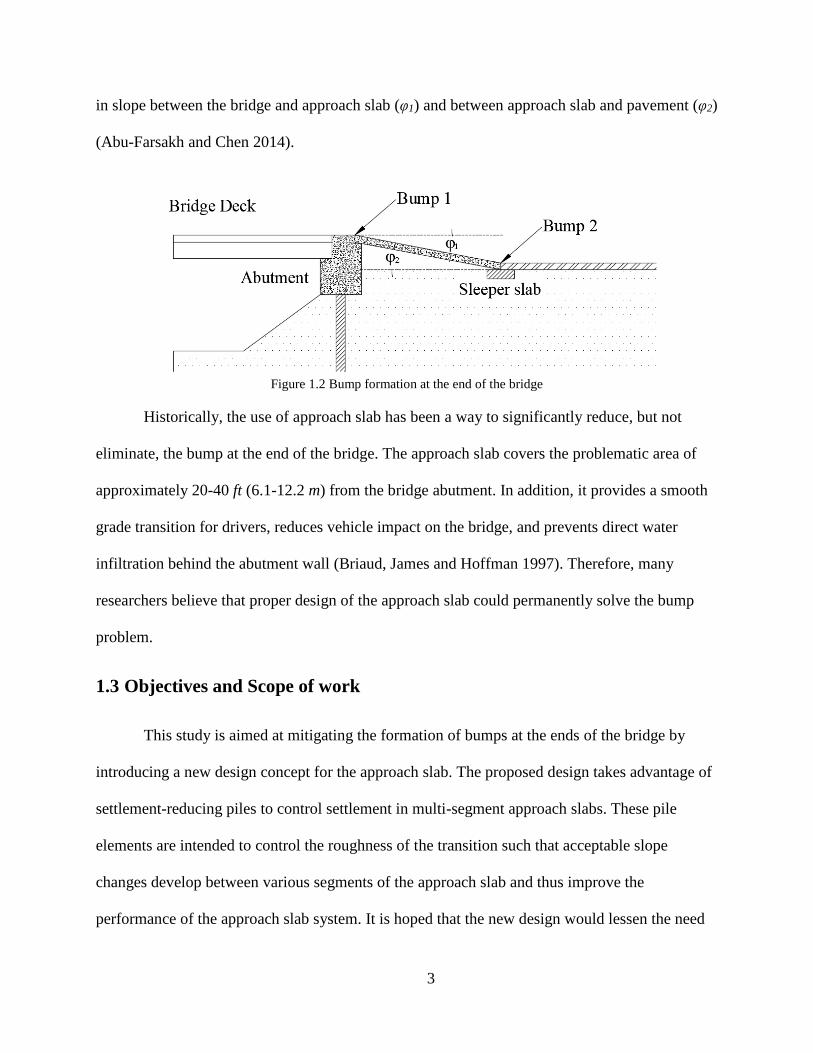
3
in slope between the bridge and approach slab (φ1) and between approach slab and pavement (φ2)
(Abu-Farsakh and Chen 2014).
Figure 1.2 Bump formation at the end of the bridge
Historically, the use of approach slab has been a way to significantly reduce, but not
eliminate, the bump at the end of the bridge. The approach slab covers the problematic area of
approximately 20-40 ft (6.1-12.2 m) from the bridge abutment. In addition, it provides a smooth
grade transition for drivers, reduces vehicle impact on the bridge, and prevents direct water
infiltration behind the abutment wall (Briaud, James and Hoffman 1997). Therefore, many
researchers believe that proper design of the approach slab could permanently solve the bump
problem.
1.3 Objectives and Scope of work
This study is aimed at mitigating the formation of bumps at the ends of the bridge by
introducing a new design concept for the approach slab. The proposed design takes advantage of
settlement-reducing piles to control settlement in multi-segment approach slabs. These pile
elements are intended to control the roughness of the transition such that acceptable slope
changes develop between various segments of the approach slab and thus improve the
performance of the approach slab system. It is hoped that the new design would lessen the need

4
for repetitive maintenance operations and thus lessen maintenance costs. Ultimately, the new
design may offer an effective design approach to limit the impact of any bump formations to
acceptable levels.
The proposed work plan to achieve to the objectives of this research includes the
following tasks:
1- Conduct comprehensive literature review of previous work to collect information
regarding the causes and mitigation techniques regarding bump formation at the ends
of the bridge.
2- Examine state practices related to the design and construction of the approach slabs
and approach areas. These include the preferred methods and configuration of the
approach slab, backfill and embankment fill.
3- Develop soil-structure finite element models that could predict soil settlement behind
bridge abutments. This includes:
a. Conducting verification analyses to compare field-measured soil settlements
with the developed finite element model.
b. Developing two baseline finite element models to examine several aspects
related to the construction of the bridge approach areas, and to assess the
severity of the bump at the end of the bridge under various soil conditions.
These aspects include the natural soil type and height, embankment soil type
and height, side slope of embankment fill, backfill soil compaction level,
slope of backfill area, erosion of backfill material, abutment type, and length
of approach slab.

5
c. Developing relationships to evaluate the long-term soil settlement profile
along a longitudinal line behind the bridge abutment.
4- Develop a soil-structure finite element model that could predict pile head settlement
for various pile-soil conditions. These include the length and size of pile, type and
height of backfill layer, type and height of embankment soil, and type and height of
natural soil. Only cast-in-place concrete piles were considered. Additionally:
a. Develop relationships to evaluate pile head settlement and pile load
distribution under various pile-soil conditions.
b. Develop criteria to select size, spacing, and length of piles to achieve
acceptable transition between the bridge and the roadway.
c. Develop procedures to achieve the desired transition profile using multi-
segment pile-supported approach slabs.
5- Verify the developed procedures and relationships using a full-scale finite element
model. This include the prediction of the longitudinal soil settlement profile, pile head
settlement, and differential settlement of the approach slab.
6- Propose design recommendations to control the settlement-induced bumps at the ends
of bridges by limiting slope changes to acceptable levels under varying soil
conditions.
1.4 Outline of Dissertation
Chapter 1 presents background of the problems associated with bridge approach slabs,
problem statement, research objectives, and scope of work.
6
Chapter 2 presents a review of previous works related to the definition, causes and
mitigation techniques for bump formation at the ends of the bridge. This chapter also reviews
previous work related to the optimum approach slab configuration.
Chapter 3 examines state practices regarding the approach slabs and approach areas.
These include the preferred methods and configurations of the approach slab, backfill and
embankment fill.
Chapter 4 discusses the general aspects of the development of finite element models used
in this research. These include geometry and boundary conditions, contact behavior at soil-
structure interfaces, analysis procedures, and material properties.
Chapter 5 presents simulation results for the soil settlement profiles behind bridge
abutments in longitudinal and transverse directions. Empirical relationships for predicting
settlements are also provided in this chapter.
Chapter 6 presents simulation results for the pile head settlement and axial load
distribution along the piles. Empirical relationships and design charts for predicting pile head
settlements are provided in this chapter. In addition, proposed procedures and recommendations
for the design multi-segment pile-supported bridge approach slabs are provided in this chapter.
Chapter 7 presents an overall assessment of the developed procedures and design charts
using a full-scale simulation of a multi-segment pile-supported bridge approach slab system.
Chapter 8 provides summary and conclusions of the work conducted in this study, and
provides recommendations for future research.

7
CHAPTER 2 - LITERATURE REVIEW
2.1 Definition of the bump
Two bumps could develop at the end of the bridge: one at the approach slab/bridge joint,
and the other at the approach slab/pavement interface, (Figure 1.2). These bumps can be
attributed to changes in slope between the bridge and approach slab (φ1) and between approach
slab and pavement (φ2) (Abu-Farsakh and Chen 2014).
The severity of the bump is mainly controlled by the amount of the differential settlement
of the approach slab. The differential settlement could be assessed using several methods. These
include the relative elevation, slope change, and the International Roughness Index (IRI)
(Puppala, et al. 2008).
The relative elevation is defined as the absolute vertical difference between the two ends
of the approach slab. In a survey of bridge movements, Walkinshaw (1978) noted that bridge
approaches with differential settlement of greater than or equal to 2.5 in (64 mm) were
considered annoyance to drivers. Long et al. (1999) conducted a survey of 1,181 bridges in
Illinois to assess the severity of the bump. The survey revealed that bridges with differential
settlement of 2-3 in (50-75 mm) were considered a significant issue from a rideability standpoint.
The slope change is typically referred to the rate of settlement between the bridge and the
roadway pavement. This rate can be expressed in terms of differential settlement between the
two ends of the approach slab divided by the length of the approach slab (slope of the approach
slab) (Figure 2.1). Long et al. (1999) concluded that a slope of 1/125 to 1/100 is tolerable.

8
Greater slopes would be a riding discomfort to drivers and maintenance operations are required
in such cases (Long, et al. 1999).
Figure 2.1 Slope of approach slab
The International Roughness Index (IRI) is a laser-profile-based pavement rating system
that is often used to assess the riding quality over a given road section. The IRI was modified
later to accommodate the approach slab (IRIS) with the ability to evaluate the ride quality along
the approach slab (Bakeer, Shutt, et al. 2005). Table 2.1 shows typical IRIS rating values.
Table 2.1 Proposed IRIS rating for approach slab (Bakeer, Shutt, et al. 2005)
IRIS range
in/mile (mm/km) Approach slab rating
0.00 - 247 (0.00 – 3900) Very good
254 - 500 (4000 – 7900) Good
507 - 628 (8000 – 9900) Fair
634 - 755 (10000 – 11900) Poor
760 (12000) and greater Very poor
Therefore, a differential settlement of up to 2.5 in (64 mm), slope change of 1/125, or an
IRIS value of 500 in/mile (7900 mm/km) may be considered acceptable from a ride quality
standpoint. These represent the maximum values allowed for the approach slab.
2.2 Maintenance considerations
The bump at the end of the bridge is considered a maintenance issue, since it may lead to
maintenance operations to keep it within a tolerable limit. It is inevitable that settlement would
take place underneath the approach slab over time. Therefore, bumps could develop and
complications (such as rough driving conditions and deterioration of the bridge deck and/or

9
approach slab) may arise that require maintenance operations. Repair or replacement of the
approach slab may be required in case of significant damage. Repetitive maintenance operations
negatively impact the travelling public, especially when lane closures are required.
In recent years, several studies conducted surveys that aim to assess the significance of
this problem as perceived by transportation agencies. The following is a review these studies.
In a survey of 758 bridge approach areas in Oklahoma, Laguros et al. (1990) reported that
the bump at the end of the bridge affected about 83% of the bridges in Oklahoma. Another
survey by Hoppe (1999), which included responses from 38 State Departments of Transportation
(DOTs), concluded that 55% of the DOTs considered the bump as major maintenance problem.
Table 2.2 shows the result of this survey. Dupont et al. (2002) conducted a survey of DOTs. In
that survey, one question asked whether the bump at the end of the bridge was a major
maintenance problem. The survey revealed that 48% of the DOTs considered it a major
maintenance problem, 28% indicated that the bump was not an issue, and the remaining 24%
indicated that it was an issue in some cases.

10
Table 2.2 The significance of the bump at the end of the bridge (Hoppe 1999)
State Significance State Significance
AZ Not significant MO Significant
CA Significant MT Significant
CT Moderate ND Significant
DE Significant NE Significant
FL Moderate NH Not Significant
GA Significant NJ Moderate
ID Significant NM Significant
IN Moderate NY Moderate
IA Moderate OH Moderate
IL Significant OK Significant
KS Significant OR Significant
KY Significant SC Significant
LA Significant SD Significant
MA Moderate TX Not Significant
MD Moderate VT Not Significant
ME Not significant VA Moderate
MI Moderate WA Significant
MN Significant WI Significant
MS Significant WY Not Significant
Typically, DOTs require biannual inspections of all bridges through which maintenance
operations are recommended based on the findings. Examples of needed maintenance operations
for the approach area include leveling, mudjacking, building an approach slab (if not used
originally), improving drainage, and implementation of soil improvement techniques. The type
of maintenance, frequency of repairs, and the type of materials and equipment needed are critical
factors in the total maintenance cost during the lifetime of the bridge. The average maintenance
cost for repairing the bump at the end of the bridge in the United States is on the order of $667
per year per bridge (1997 dollars) (Briaud, James and Hoffman 1997). Dupont and Allen (2002)
conducted an evaluation of maintenance operations in the state of Kentucky. It was reported that
repairing the bump at the end of bridge cost approximately $2000 per year per bridge.
Furthermore, Dupont and Allen (2002) recommended several practices that aim to reduce the
maintenance cost and formation of the bump. Table 2.3 summarizes those recommendations.
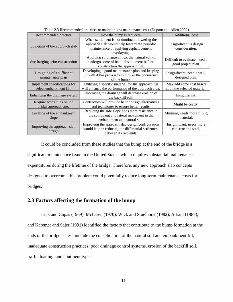
11
Table 2.3 Recommended practices to maintain low maintenance cost (Dupont and Allen 2002)
Recommended practice How the bump is reduced? Additional cost
Lowering of the approach slab
When settlement is not dominant, lowering the
approach slab would help toward the periodic
maintenance of applying asphalt cement
overlaying.
Insignificant, a design
consideration.
Surcharging prior construction
Applying surcharge allows the natural soil to
undergo some of its total settlement before
construction the approach fill.
Difficult to evaluate, need a
good project plan.
Designing of a sufficient
maintenance plan
Developing a good maintenance plan and keeping
up with it has proven to minimize the occurrence
of the bump.
Insignificant, need a well-
designed plan.
Implement specifications for
select embankment fill.
Utilizing a specific material for the approach fill
will enhance the performance of the approach area.
May add some cost based
upon the selected material.
Enhancing the drainage system Improving the drainage will decrease erosion of
the backfill soil. Insignificant.
Require warranties on the
bridge approach area
Contractors will provide better design alternatives
and techniques to ensure better results. Might be costly.
Leveling of the embankment
slope
Reducing the side slope adds more resistance to
the settlement and lateral movement in the
embankment and natural soil.
Minimal, needs more filling
material.
Improving the approach slab
design
Improving the approach slab design/configuration
would help in reducing the differential settlement
between its two ends.
Insignificant, needs more
concrete and steel.
It could be concluded from these studies that the bump at the end of the bridge is a
significant maintenance issue in the United States, which requires substantial maintenance
expenditures during the lifetime of the bridge. Therefore, any new approach slab concepts
designed to overcome this problem could potentially reduce long-term maintenance costs for
bridges.
2.3 Factors affecting the formation of the bump
Irick and Copas (1969), McLaren (1970), Wick and Stoelhorst (1982), Adrani (1987),
and Karemer and Sajer (1991) identified the factors that contribute to the bump formation at the
ends of the bridge. These include the consolidation of the natural soil and embankment fill,
inadequate construction practices, poor drainage control systems, erosion of the backfill soil,
traffic loading, and abutment type.

12
Laguros, Zaman, and Mahmood (1986) surveyed all state DOTs. The survey concluded
that the types of the natural soil and embankment fill along with the construction method were
the most significant factors affecting the formation of the bump at the ends of the bridge.
Furthermore, it was noted that factors such as frost heave and freeze thaw cycles, lateral
movement of the abutment, and abutment type influenced the bump formation. In a second phase
of the same study, Laguros, Zaman, and Mahmood (1990) reported that the age of the approach
area, type of the abutment, height of the embankment, drainage behind the abutment wall, traffic
volume, and skewness of the bridge were among the factors that influenced the bump formation.
A synthesis study of 48 states, conducted by Briaud, James and Hoffman (1997),
discussed various aspects related to the bump at the ends of the bridge. This study identified the
most common factors that contribute to the formation of the bump. These factors include the
height of the embankment, type of abutment foundation, natural soil profile, traffic volume,
thermal expansion and contraction of the bridge, precipitation, and the side slope of the approach
area. These factors and others are illustrated in Figure 2.2.
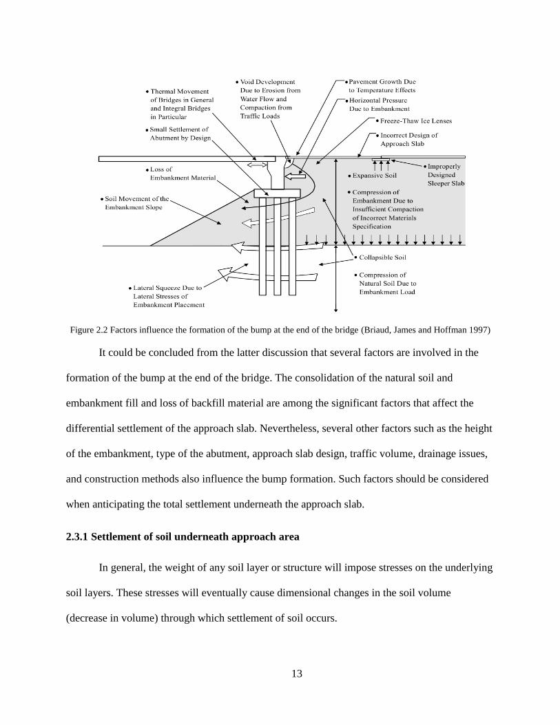
13
Figure 2.2 Factors influence the formation of the bump at the end of the bridge (Briaud, James and Hoffman 1997)
It could be concluded from the latter discussion that several factors are involved in the
formation of the bump at the end of the bridge. The consolidation of the natural soil and
embankment fill and loss of backfill material are among the significant factors that affect the
differential settlement of the approach slab. Nevertheless, several other factors such as the height
of the embankment, type of the abutment, approach slab design, traffic volume, drainage issues,
and construction methods also influence the bump formation. Such factors should be considered
when anticipating the total settlement underneath the approach slab.
2.3.1 Settlement of soil underneath approach area
In general, the weight of any soil layer or structure will impose stresses on the underlying
soil layers. These stresses will eventually cause dimensional changes in the soil volume
(decrease in volume) through which settlement of soil occurs.

14
Typically, settlement of soil consists of three different stages: initial settlement
(immediate), primary compression settlement (consolidation), and secondary compression
(creep). The total settlement can be evaluated as a summation of these components as follows:
𝑆𝑡 = 𝑆𝐼 + 𝑆𝑃 + 𝑆𝑆 2-1
Where
St = Total settlement at time (t).
Si = Initial settlement.
Sp = Settlement due to primary compression (consolidation).
Ss = Settlement due to secondary compression (creep).
The initial settlement (Si) takes place immediately after the load is applied on the soil
mass. This is caused by shear strain and the decrease of void ratio between soil particles. In
bridge construction, the initial settlement typically develops before the construction of the
approach slab. This stage is influenced by the degree of saturation of the soil, where partially
saturated soils tend to produce greater initial settlement than fully saturated soils (Puppala, et al.
2008, McCarthy 2007).
The primary settlement (Sp) is typically referred to as time-dependent settlement
(consolidation). It takes place when stress gradually transfers from water to soil particles
(dissipation of water). In granular soils, such as sands and gravels, this stage occurs rapidly, due
to the high permeability of such soils. However, in fine soils, such as clays and silts, this stage
could take several years due to the low permeability of such soils (Puppala, et al. 2008,
McCarthy 2007).

15
The secondary settlement (Ss) is also time-depended in which the volume of the soil is
decreased due to creep. In this stage, the void ratio of the soil mass decreases further under
constant application of the load. The secondary settlement is usually neglected in granular soils.
However, in highly plastic fine soils, the secondary compression settlement could be as
significant as the primary settlement (Puppala, et al. 2008, McCarthy 2007).
Wahls (1990) noted that a significant portion of the stress imposed on the natural soil
develops from the self-weight of the embankment fill. Figure 2.3 compares the vertical stress
imposed on the natural soil by embankment fill and bridge abutment.
Figure 2.3 Vertical stress imposed on natural soil by embankment fill and abutment (Wahls 1990)
It is well known that post-construction settlement issues are more dominate in cohesive
soils. Accordingly, it is very important to investigate cohesive natural soils before constructing
the embankment fill. Doing so would help anticipate the total settlement underneath the approach
slab (Wahls 1990).
2.3.2 Embankment fill
The embankment fill plays a significant role when it comes to the bump formation at the
ends of the bridge as it is the source of the stress imposed on the natural soil. The embankment
fill area could be defined as the area extending from the back of the abutment wall to an average

16
distance of about 100 ft (31 m). This area includes the backfill material, approach slab, and a
portion of the roadway pavement (Puppala, et al. 2008, White, et al. 2005). Within the approach
slab, greater differential settlement is expected when tall embankment fills are employed. Long
et al. (1999) classified the height of the embankment fill into: low He ≤ 10 ft ( 3.0 m), medium 10
ft ( 3.0 m) ≤ He ≤ 26 ft ( 8.0 m), and high He > 26 ft ( 8.0 m), where He is the height of the
embankment fill.
The embankment fill undergoes global as well as local settlement over time. Global
settlement takes place in deeper natural soil layers due to consolidation. On the other hand,
erosion, movement of the abutment wall, and compression of the embankment fill are the main
contributors to the local settlement (Washington State Department of Transportation 2015).
Typically, an embankment fill, such as non-cohesive granular soil that is compacted well results
in little or negligible settlement. However, low cost fill materials that are readily and locally
available are widely used, especially when high embankment fills are needed. Frequently, the
readily-available fill contains significant clay materials, which could result in significant time-
dependent consolidation, even with good compaction (Briaud, James and Hoffman 1997,
McLaren 1970, Dupont and Allen 2002). According to Hoppe (1999), 49% of the DOTs require
embankment fills that are highly permeable and non-plastic, while the remaining DOTs may
permit the use of readily available highway embankment fill that might not perform
satisfactorily.
The side slope of the embankment fill, oriented in the transverse direction (see Figure
5.4), is another factor that influences the settlement. Typically, the embankment fill is built with
a slope of 1:2 (1 vertical to 2 horizontal) (see Chapter 3). Allen and Meade (1988), Kramer and

17
Sajer (1991), and Dupont and Allen (2002) reported that leveling the slope of the embankment
(by constructing wing walls) adds more resistance to settlement and lateral movement of the soil.
2.3.3 Abutment
The abutment is a vital part of the bridge system that carries a large portion of the bridge
load and provides vertical and lateral support at the end of the bridge. The type of the abutment
(wall or stub), abutment foundation type, and movement of the abutment influence the formation
of the bump at the end of the bridge. An overview of these elements will be presented in the
following sections.
2.3.3.1 Abutment type
There are several types of abutment that are commonly used on bridges. For the purposes
of this study, the wall and stub abutments will be examined.
The wall abutment consists of a wall that extends the full height of the embankment fill
(Figure 2.4). The wall abutment typically experiences higher lateral earth pressure (induced by
the full height of the embankment fill) when compared with other abutment types (Briaud, James
and Hoffman 1997, Wahls 1990).
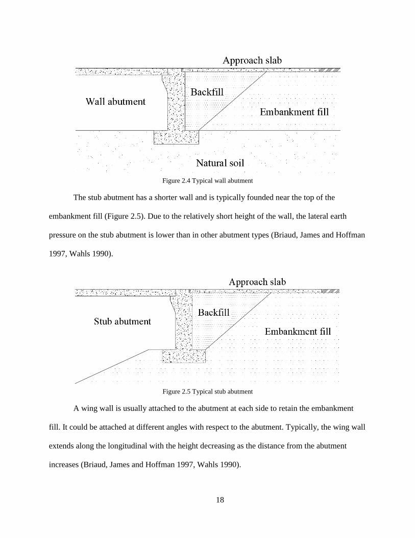
18
Figure 2.4 Typical wall abutment
The stub abutment has a shorter wall and is typically founded near the top of the
embankment fill (Figure 2.5). Due to the relatively short height of the wall, the lateral earth
pressure on the stub abutment is lower than in other abutment types (Briaud, James and Hoffman
1997, Wahls 1990).
Figure 2.5 Typical stub abutment
A wing wall is usually attached to the abutment at each side to retain the embankment
fill. It could be attached at different angles with respect to the abutment. Typically, the wing wall
extends along the longitudinal with the height decreasing as the distance from the abutment
increases (Briaud, James and Hoffman 1997, Wahls 1990).

19
Proper compaction of soil near the abutment backwall is difficult to achieve due to the
confined space in that area. Hoppe (1999) reported that 50% of the DOTs have had difficulty in
obtaining the specified degree of backfill compaction near the abutment wall. Consequently, as
this area becomes larger, the soil would become more vulnerable to settlement and/or washout.
This could lead to the formation of a void underneath the approach slab.
2.3.3.2 Abutment foundation type
The abutment wall is either supported on piles or on spread footing. The type of the
foundation influences the differential settlement of the approach slab, since one end of the
approach slab is supported on the bridge abutment. Typically, pile-supported abutments induce
negligible settlement. This in turn leads to great differential settlement of the approach slab, thus,
increasing the chance for forming bumps. On the other hand, abutments that are supported on
spread footings tend to generate higher settlement. This in turn could lead to low differential
settlement in the approach slab and lessen the chances of the bump formation (Laguros, Zaman
and Mahomood 1990).
2.3.3.3 Movement of the abutment
The movement of the abutment affects both the bridge and the embankment fill and can
influence the formation of the bump. In integral bridges, thermal expansion and/or contraction of
the bridge causes the abutment wall to move laterally towards or away from the adjacent soil.
These cyclic movements induce large horizontal displacement in the backfill soil, resulting in a
formation of a void underneath the approach slab. Figure 2.6 shows the mechanism of the void
formation due to the abutment movement (Puppala, et al. 2008).
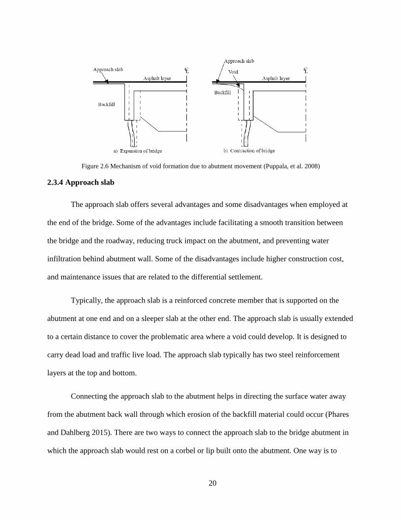
20
Figure 2.6 Mechanism of void formation due to abutment movement (Puppala, et al. 2008)
2.3.4 Approach slab
The approach slab offers several advantages and some disadvantages when employed at
the end of the bridge. Some of the advantages include facilitating a smooth transition between
the bridge and the roadway, reducing truck impact on the abutment, and preventing water
infiltration behind abutment wall. Some of the disadvantages include higher construction cost,
and maintenance issues that are related to the differential settlement.
Typically, the approach slab is a reinforced concrete member that is supported on the
abutment at one end and on a sleeper slab at the other end. The approach slab is usually extended
to a certain distance to cover the problematic area where a void could develop. It is designed to
carry dead load and traffic live load. The approach slab typically has two steel reinforcement
layers at the top and bottom.
Connecting the approach slab to the abutment helps in directing the surface water away
from the abutment back wall through which erosion of the backfill material could occur (Phares
and Dahlberg 2015). There are two ways to connect the approach slab to the bridge abutment in
which the approach slab would rest on a corbel or lip built onto the abutment. One way is to

21
extend reinforcing steel dowels from the bridge deck into the approach slab. Another way
involves placing inclined bars to form an integrated connection between the approach slab and
the abutment. In both ways, the bars are meant to restrict the relative horizontal movement
between the approach slab and the bridge abutment while allowing the slab to rotate. The
approach slab could also have no positive connection (no steel bars across the interface) with the
superstructure (Greimann, et al. 2008). In such cases, the approach slab could gradually separate
from the bridge.
The design parameters for the approach slab can significantly influence the bump at the
end of the bridge. The length and thickness of the approach slab, type of support at the approach
slab/pavement connection, and type of connection to the bridge are important factors that should
be taken into consideration in any approach slab design. The design of the approach slab must
assure that the slab can withstand the anticipated differential settlement and that the resulting
slope is within tolerable limits (see Section 2.1).
2.3.5 Drainage
Utilizing proper drainage systems can help control the erosion of the backfill material and
reduce hydrostatic pressure behind the abutment wall. Adequate drainage system should keep the
water away from behind the abutment. Poor drainage can lead to slope instability, slope
subsidence, and significant damage to the bridge abutment and approach slab; all of which are
factors contributing to the formation of the bump at the end of the bridge. In that manner, both
surface and subsurface drainage should be counted for in the bridge approach system. One
approach to keep the runoff water away from the backfill involves using gutters and paved
ditches along both sides of the pavement (Briaud, James and Hoffman 1997, Lenke 2006).
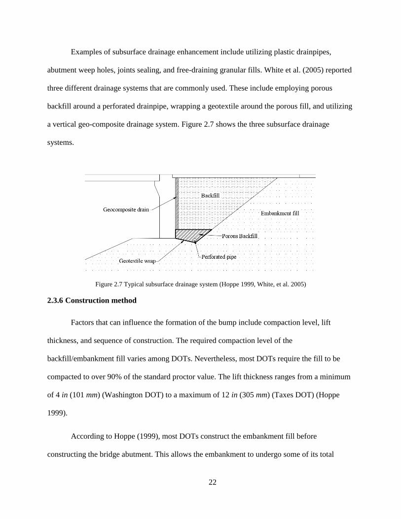
22
Examples of subsurface drainage enhancement include utilizing plastic drainpipes,
abutment weep holes, joints sealing, and free-draining granular fills. White et al. (2005) reported
three different drainage systems that are commonly used. These include employing porous
backfill around a perforated drainpipe, wrapping a geotextile around the porous fill, and utilizing
a vertical geo-composite drainage system. Figure 2.7 shows the three subsurface drainage
systems.
Figure 2.7 Typical subsurface drainage system (Hoppe 1999, White, et al. 2005)
2.3.6 Construction method
Factors that can influence the formation of the bump include compaction level, lift
thickness, and sequence of construction. The required compaction level of the
backfill/embankment fill varies among DOTs. Nevertheless, most DOTs require the fill to be
compacted to over 90% of the standard proctor value. The lift thickness ranges from a minimum
of 4 in (101 mm) (Washington DOT) to a maximum of 12 in (305 mm) (Taxes DOT) (Hoppe
1999).
According to Hoppe (1999), most DOTs construct the embankment fill before
constructing the bridge abutment. This allows the embankment to undergo some of its total

23
settlement before opening the bridge to the public. Typically, the type of abutment influences the
order of construction. When a stub abutment is employed, the embankment is typically construed
first, and the abutment is placed near the top of the embankment. However, when a wall
abutment is employed, the abutment is constructed first (Hoppe 1999).
2.3.7 Traffic volume
The average daily traffic (ADT), vehicle speed and weight, and number of cycles of
loading can influence the formation of the bump at the end of the bridge when no approach slab
is employed. Based on the compressibility and/or level of compaction of the soil, the approach
fill could be further compressed due to heavy traffic loading. When an approach slab is
employed, it significantly decreases the severity of the bump caused by this void. The approach
slab is usually designed to sustain full traffic loading in a free span, even if it has lost contact
with the underlying soil. In such cases, the traffic volume, and vehicle velocity would not have
any effect on the formation of the bump at the end of the bridge (Dupont and Allen 2002,
Puppala, et al. 2008, Lenke 2006).
2.3.8 Bridge skew
Laguros, Zaman, and Mahmood (1990) reported that skewed approach fills were
associated with higher settlement than non-skewed approach fills. However, a relationship
between the settlement and the degree of skewness could not be established.
Nassif et al. (2002), conducted finite element analyses to evaluate the performance of
skewed approach slabs under differential settlement. It is reported that skewed approach slabs
developed higher tensile stresses than straight approach slabs.

24
Cai, Voyiadjis and Shi (2005) agreed with the findings of Nassif et al. (2002), and
showed that, in skewed approach slabs, the tensile stress distribution along the long side of the
approach slab increases as the differential settlement increases (Figure 2.8).
Figure 2.8 Distribution of tensile stress in skewed approach slab (Cai, Voyiadjis and Shi 2005)
2.4 Mitigation techniques
The mitigation techniques that are typically used after formation of the bump are
classified into four groups:
• Improvement of the natural soil;
• Improvement of the embankment fill;
• Enhancement of the drainage and erosion control system; and
• Improvement of the approach slab design.
Wick and Stoelhorst (1982) recommended several practices to control the differential
settlement of the approach slab. These include supporting the approach slab/pavement end with a
sleeper slab, cement stabilization of the embankment fill, and implementation of drainage control
systems.

25
Karemer and Sajer (1991), made several recommendations to minimize the differential
settlement of the approach slab. One recommendation was to level out the slope of the
embankment with wing walls. This was intended to reduce creep settlement of the natural soil,
especially of highly plastic and/or organic soils. They also recommended that good quality
control of embankment materials and compaction specifications would help reduce the
settlement of the embankment fill. Another recommendation was to straighten the backwall face
of the abutment. This was intended to simplify the compaction process near the abutment wall.
Briaud, James and Hoffman (1997) made several recommendations regarding the design,
construction and maintenance of the bridge approach area to minimize or eliminate the bump.
These recommendations are summarized as follows:
• Utilizing an approach slab particularly when excessive settlement is anticipated.
• Implementation of an adequate drainage and erosion control system.
• Performing routine inspection and maintenance to enhance performance of the
approach area and improve the overall rideability.
Hoppe (1999) conducted a survey of various states regarding issues related to the
approach slab. The objective of this study was to compare various state practices including those
adopted by Virginia DOT. Ultimately, design recommendations were made for mitigating the
differential settlement of the approach slab. The recommendations are listed below and
illustrated in Figure 2.9:
• Utilizing a full-width, curb-to-curb, approach slab. This was intended to lessen
the void formation due to water seepage.

26
• Appropriate design of the approach slab. The length of the approach slab is
typically designed to ensure gradual transition between the bridge and the
roadway.
• Lowering the approach slab below the base course level. This was aimed at ease
of placement of future asphalt overlays. The Virginia DOT design required the
approach slab to be lowered 28 in (700 mm) below the road surface (Figure 2.9).
• Pre-cambering of the embankment fill for a distance equal to the length of the
approach slab (Figure 2.9). This was intended to account the post-construction
settlement.
Figure 2.9 Proposed approach slab configuration (Hoppe 1999)
A later study by Dupont and Allen (2002) agreed with the Hoppe (1999)
recommendations and made recommendations for reducing differential settlement. These
recommendations were discussed in section 2.2 (see Table 2.3).
Mistry (2005) recommended several practices regarding the design of the approach slab.
Some of the recommendations are summarized below.

27
• Cooperation between structural and geotechnical engineers, especially in the
decision to use an approach slab. The decision should be based on long-term
performance and life cycle cost, instead of the initial cost of the project.
• Standardized use of a sleeper slab. This was meant to prevent excessive
settlement and cracking at the approach slab/pavement connection.
• Using a well-drained granular backfill material to accommodate expansion and
contraction of the bridge abutment, especially in integral abutment bridges.
• Connecting the approach slab to the superstructure with a hinge connection.
• Providing two layers of polyethylene sheets or fabric underneath the approach
slab to reduce friction caused by the horizontal movement of integral abutments.
• Limiting skew angle to 30 degrees to minimize the magnitude and lateral
eccentricity of the longitudinal forces.
2.5 Optimum approach slab configuration
This section is a review of previous studies that proposed various approach slab
configurations to mitigate the formation of the bump and to improve the overall ride quality of
the bridge approach area.
Wong and Small (1994) proposed utilizing an angled approach slab that is sloping down
beneath the pavement (Figure 2.10). According to their findings, the formation of the bump was
attributed to the abrupt change in the material stiffness between the approach slab and the
pavement. Consequently, it was anticipated that this slab configuration would result in a
smoother and more gradual change in the material stiffness.

28
Figure 2.10 proposed approach slab (Wong and Small 1994)
Physical models of pavements and approach slabs have been examined in a laboratory-
scale test track. Three different approach slab orientations of 0, 5, and 10 degrees have been
evaluated. As a result, it was concluded that the severity of bump decreases as the oriented angle
of the approach slab increases. Figure 2.11 shows the surface deformation of the three
orientations used in the study.
Figure 2.11 Surface deformation of angled slabs (Wong and Small 1994)
Seo, Ha and Briaud (2002) examined the performance of the approach slabs for the Texas
DOT. The typical approach slab had a thickness of 12 in (305 mm) and consisted of two 20 ft
(6.1 m) spans. The slab was designed to be supported on the abutment wall, embankment fill,
support slab and sleeper slab (Figure 2.12). In addition, a wide flange steel beam was employed
at the end of approach slab to accommodate the thermal movements of the pavement.

29
Figure 2.12 Current Taxis DOT approach slab (Seo, Ha and Briaud 2002)
Finite element analyses were carried out in this study. As a result, the following
conclusion were drawn:
• The differential settlement between the bridge and the embankment fill is
unavoidable when the abutment is supported on piles.
• The abutment wall has a significant influence on the differential settlement. The
friction between the abutment wall and the adjacent backfill soil restricts some of
the soil in the vicinity of the abutment wall, while the soil away remains
unsupported and settles more.
• The transition zone, where most of the settlement occurs, is approximately 40 ft
(12.2 m) away from the back of the abutment wall.
• The width of the support slab, sleeper slab, and the height of the embankment
were found to influence the differential settlement of the approach slab. The
optimum width of the support slab and sleeper slab was found to be 5 ft (1.5 m).
Seo, Ha and Briaud (2002) proposed a new approach slab concept to simplify the
construction, reduce cost, and lessen the need for good compaction in the backfill area. The
proposed approach slab was a single 20 ft (6.1 m) slab supported on the abutment wall at one end
and a sleeper slab at the other end (Figure 2.13). The slab was designed to carry the loads

30
without the support of the soil. The wide flange steel beam was kept in this design to
accommodate thermal movement of the pavement.
After examining the proposed approach slab, the following conclusion were drawn;
• The single-span approach slab has performed better and resulted in a smaller
bump than the current two-span approach slab.
• Highly compacted embankment soils result in a smaller bump at the approach
slab/pavement end.
Figure 2.13 Single span approach slab (Seo, Ha and Briaud 2002)
Cai, Voyiadjis and Shi (2005) performed a numerical study of the performance of two
different approach slab types (flat versus ribbed) under a given differential settlement. The
presumed settlement profiles employed in the analysis were based on a partial embankment
contact with the approach slab. This study was aimed at establishing a relationship between the
internal forces and deformation in the slab with some of the design parameters including length
and thickness. Figure 2.14 shows the layout used in their study.

31
Figure 2.14 Layout of the finite element analysis (Cai, Voyiadjis and Shi 2005)
As a result of the study, it was concluded that the flat approach slab was more applicable
for short spans, i.e. 20 to 40 ft (6.1 to 12.2 m) because the longer spans required greater
thickness. In such cases, ribbed approach slab was preferred. The slab on beam behavior in
ribbed slabs would significantly reduce the internal stresses and deformation, thus reducing the
amount of reinforcement. Figures 2.15 and 2.16 show the stress distribution in a flat and ribbed
approach slab with a 6 in (152 mm) embankment settlement.

32
Figure 2.15 Stress distribution in flat slab (Cai, Voyiadjis and Shi 2005)
Figure 2.16 Stress distribution in ribbed slab (Cai, Voyiadjis and Shi 2005)
The connection between the approach slab and the bridge abutment was also investigated
in their study. As a result, it was recommended that an inclined bar be used to connect the
approach slab with the abutment. This connection would allow free rotation between the
approach slab and abutment while restricting the relative horizontal movement between them.
Abu-Farsakh and Chen (2014) examined the performance of a proposed approach slab
that relied upon increasing its rigidity as well as reinforcing the embankment soil underneath the
sleeper slab. The rigidity of the proposed approach slab was increased by increasing its thickness
to 16 in (406 mm) and utilizing more steel reinforcement. The reinforcing of the embankment
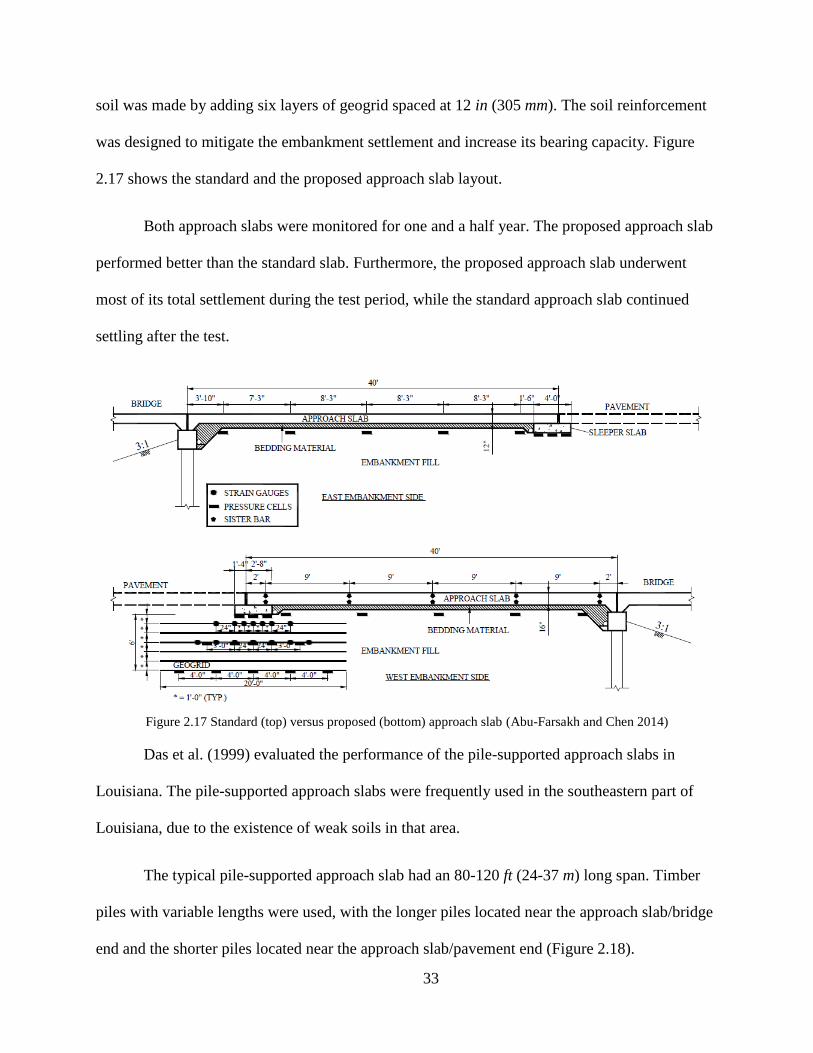
33
soil was made by adding six layers of geogrid spaced at 12 in (305 mm). The soil reinforcement
was designed to mitigate the embankment settlement and increase its bearing capacity. Figure
2.17 shows the standard and the proposed approach slab layout.
Both approach slabs were monitored for one and a half year. The proposed approach slab
performed better than the standard slab. Furthermore, the proposed approach slab underwent
most of its total settlement during the test period, while the standard approach slab continued
settling after the test.
Figure 2.17 Standard (top) versus proposed (bottom) approach slab (Abu-Farsakh and Chen 2014)
Das et al. (1999) evaluated the performance of the pile-supported approach slabs in
Louisiana. The pile-supported approach slabs were frequently used in the southeastern part of
Louisiana, due to the existence of weak soils in that area.
The typical pile-supported approach slab had an 80-120 ft (24-37 m) long span. Timber
piles with variable lengths were used, with the longer piles located near the approach slab/bridge
end and the shorter piles located near the approach slab/pavement end (Figure 2.18).

34
Figure 2.18 Pile-supported approach slab (Bakeer, Shutt, et al. 2005)
The performance of the pile-supported approach slab was evaluated by visual inspection,
surveys and assessment of road surface condition. It was noted that while many pile-supported
approach slabs performed well, many others settled enough to develop a bump at the approach
slab/pavement end. The reason for such settlement was attributed mainly to the unanticipated
negative skin friction (downdrag force) imposed on the piles. Accordingly, it was pointed out
that soil should undergo most of its consolidation before installing the piles to overcome the
negative skin friction.
35
CHAPTER 3 - STATES PRACTICES RELATED TO APPROACH
SLABS
As discussed in Chapter 2, the design parameters of the approach slab and approach area
have a significant effect on the bump formation at the ends of the bridge. This include the
configuration of the approach slab, connection of the approach slab to superstructure, support
type at the approach slab/pavement end, backfill material, and side slope of the embankment fill.
In this phase of the study, an extensive examination of bridge manuals/guidelines published by
all DOTs was conducted. The objective was to understand and compare the current practices (as
of 2017) related to the design of the approach slab and the approach area.
An examination of the bridge manuals (including standard drawings) was carried out and
practices relevant to the design criteria and parameters of the approach slab and approach area
were retrieved. These include the state’s preference for utilizing an approach slab at the end of
the bridge, support type at the approach slab/pavement connection, approach slab configuration
with skewed bridges, details of connection to the superstructure, approach slab dimensions
(length and thickness), and other information related to the approach area.
3.1 Approach slab preference
Approach slabs are typically utilized for new bridges under all conditions. Nevertheless,
some of the DOTs require certain conditions before requiring the use of an approach slab. Some
of these conditions include the superstructure length, height of the embankment, adjacent
roadway pavement type, abutments type, average daily traffic (ADT), and average annual daily
traffic (AADT). For instance, Colorado DOT provides the following conditions:

36
• The superstructure length is over 250 ft (76 m).
• The adjacent roadway pavement is concrete.
• When high embankment fills are used.
• When the district requests it.
• All post-tensioned structures.
Data from bridge manuals (Table 3.1 and Figure 3.1) show that approximately 41% of the
DOTs prefer the use of the approach slab for all bridges, while 22% specify certain conditions
before employing the approach slab. Roughly 2% do not prefer the use of the approach slab;
however, their practice is to design the bridge abutment for future possibility of adding an
approach slab. The remaining 35% did not mention any preference in utilizing an approach slab
at the ends of the bridge.
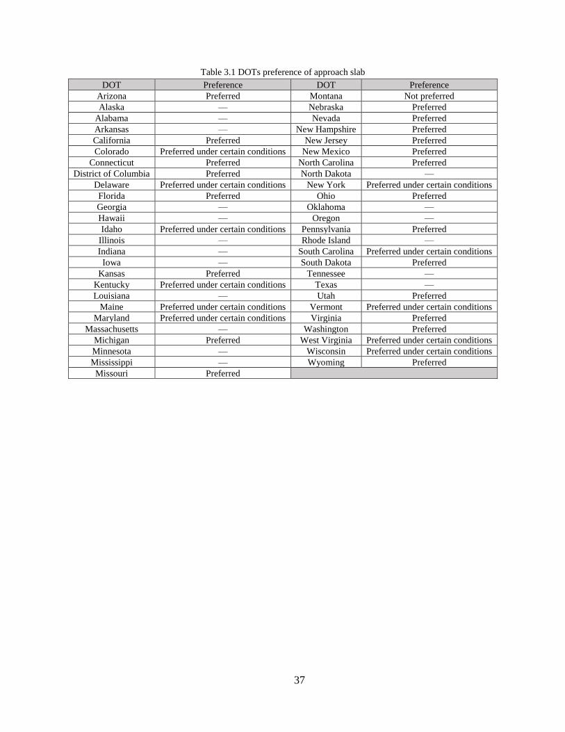
37
Table 3.1 DOTs preference of approach slab
DOT Preference DOT Preference
Arizona Preferred Montana Not preferred
Alaska — Nebraska Preferred
Alabama — Nevada Preferred
Arkansas — New Hampshire Preferred
California Preferred New Jersey Preferred
Colorado Preferred under certain conditions New Mexico Preferred
Connecticut Preferred North Carolina Preferred
District of Columbia Preferred North Dakota —
Delaware Preferred under certain conditions New York Preferred under certain conditions
Florida Preferred Ohio Preferred
Georgia — Oklahoma —
Hawaii — Oregon —
Idaho Preferred under certain conditions Pennsylvania Preferred
Illinois — Rhode Island —
Indiana — South Carolina Preferred under certain conditions
Iowa — South Dakota Preferred
Kansas Preferred Tennessee —
Kentucky Preferred under certain conditions Texas —
Louisiana — Utah Preferred
Maine Preferred under certain conditions Vermont Preferred under certain conditions
Maryland Preferred under certain conditions Virginia Preferred
Massachusetts — Washington Preferred
Michigan Preferred West Virginia Preferred under certain conditions
Minnesota — Wisconsin Preferred under certain conditions
Mississippi — Wyoming Preferred
Missouri Preferred

38
Figure 3.1 DOTs preference regarding use of approach slab
3.2 Approach slab/pavement end support
The approach slab/pavement end is usually supported on the embankment soil (soil
support), sleeper slab (Figure 3.2), or a thickened slab edge at the end of the approach slab
(Figure 3.3). Typically, a sleeper slab or a thickened edge is utilized when the adjacent roadway
pavement is rigid (concrete roadway). This aims to mitigate the abrupt change between the
approach slab and the roadway pavement. The South Carolina DOT defines the sleeper slab as “a
foundation slab, inverted tee-beam or L-beam placed transversely supporting the end of the
approach slab away from the bridge. Sleeper slabs should be used to provide an off-bridge joint
at the end of the approach slab”
35%
2%
22%
41%
Approach slab preference
Not mentioned Not preferred Preferred under conditions Preferred at all bridges

39
Figure 3.2 Typical approach slab supported on sleeper slab
Figure 3.3 Typical approach slab with thickened edge
Data from bridge manuals (Table 3.2 and Figure 3.4) show that approximately 51% of the
DOTs use only sleeper slab, 4% use only thickened edge, and 6% use either sleeper slab or
thickened edge (design decision) to support the end of the approach slab at the roadway
pavement. Roughly, 20% of the DOTs rely on the embankment fill to provide the support for the
approach slab. The remaining 19% did not mention the support type at the approach
slab/pavement end.

40
Table 3.2 Approach slab/pavement end support type
DOT Support type at end of BAS DOT Support type at end of BAS
Arizona Sleeper slab Montana —
Alaska — Nebraska Sleeper slab
Alabama Sleeper slab/Thickened edge Nevada Sleeper slab
Arkansas Sleeper slab New Hampshire Sleeper slab
California Fill support New Jersey Sleeper slab
Colorado Sleeper slab New Mexico Sleeper slab
Connecticut Fill support North Carolina Sleeper slab
District of Columbia Sleeper slab North Dakota —
Delaware Sleeper slab/Thickened edge New York Sleeper slab
Florida — Ohio Fill support
Georgia Fill support Oklahoma Fill support
Hawaii — Oregon Fill support
Idaho Sleeper slab Pennsylvania Sleeper slab
Illinois Sleeper slab Rhode Island Sleeper slab
Indiana Sleeper slab/Thickened edge South Carolina Sleeper slab
Iowa Thickened edge South Dakota Sleeper slab
Kansas Sleeper slab Tennessee Sleeper slab
Kentucky Fill support Texas Sleeper slab
Louisiana Fill support Utah Sleeper slab
Maine — Vermont —
Maryland — Virginia Fill support
Massachusetts Thickened edge Washington Fill support
Michigan Sleeper slab West Virginia —
Minnesota Sleeper slab Wisconsin Sleeper slab
Mississippi — Wyoming Sleeper slab
Missouri Sleeper slab

41
Figure 3.4 Approach slab/pavement end support type
3.3 Approach slab configuration with skewed bridges
Two approach slab configurations could be used along with skewed bridges. The
approach slab/pavement end could be made parallel to the skewed bridge or squared off.
Typically, the decision for employing one configuration over the other would be based on the
adjacent pavement type along with the skew angle. Frequently, the parallel approach
slab/pavement end is employed when the adjacent pavement is flexible (asphalt pavement), and
when the skew angle of the bridge is less than 30 degrees. The squared off approach
slab/pavement end is employed when the adjacent pavement is rigid (concrete pavement), and
when the skew angle of the bridge is greater than 30 degrees. Nevertheless, some DOTs would
use either configuration regardless of the pavement material.
20%
20%
51%
4%6%
Support type at approach slab/pavement end
Not mentioned No Support Sleeper Slab Thickened edge Combination

42
Data from bridge manuals (Table 3.3 and Figure 3.5) show that approximately 33% of the
DOTs employ the parallel approach slab/pavement end when the bridge is skewed, 18% employ
the squared off approach slab/pavement end, and 20% use one configuration over the other based
on the adjacent pavement type and/or the skew angle. The remaining 29% did not mention the
approach slab configuration with skewed bridges.
Table 3.3 Approach slab/Pavement end configuration with skewed bridges
DOT Approach slab end configuration DOT Approach slab configuration
Arizona Pavement type/Skew degree Montana —
Alaska — Nebraska Follows skew angle
Alabama Pavement type/Skew degree Nevada Follows skew angle
Arkansas Squared off New Hampshire —
California Pavement type/Skew degree New Jersey Follows skew angle
Colorado Follows skew angle New Mexico —
Connecticut Pavement type/Skew degree North Carolina Pavement type/Skew degree
District of Columbia Follows skew angle North Dakota Squared off
Delaware — New York Pavement type/Skew degree
Florida Pavement type/Skew degree Ohio Follows skew angle
Georgia Follows skew angle Oklahoma —
Hawaii — Oregon Follows skew angle
Idaho Pavement type/Skew degree Pennsylvania Follows skew angle
Illinois Follows skew angle Rhode Island —
Indiana Squared off South Carolina —
Iowa Squared off South Dakota —
Kansas Squared off Tennessee Follows skew angle
Kentucky Follows skew angle Texas Squared off
Louisiana Squared off Utah —
Maine Follows skew angle Vermont Follows skew angle
Maryland — Virginia Follows skew angle
Massachusetts Follows skew angle Washington Squared off
Michigan Squared off West Virginia —
Minnesota Pavement type/Skew degree Wisconsin Follows skew angle
Mississippi — Wyoming Pavement type/Skew degree
Missouri —

43
Figure 3.5 Approach slab/Pavement end configuration with skewed bridges
3.4 Approach slab connection mechanism to the superstructure
Connecting the approach slab to the superstructure (through reinforcement) restricts the
relative movements between the approach slab and the abutment and allows a free rotation of the
approach slab at the approach slab/bridge interface. In addition, it allows the expansion joint to
be moved away from the wall abutment (that could reduce erosion of the backfill material).
Data from bridge manuals (Table 3.4 and Figure 3.6) show that approximately 61% of the
DOTs connect the approach slab to the superstructure and 4% use no connection mechanism
(reinforcement). Roughly 16% of the DOTs make connect or not connect based on the type of
approach slab. The remaining 19% did not mention the connection type used between the
approach slab and the superstructure.
29%
33%
18%
20%
Approach slab configuration with skewed bridges
Not mentioned Follow skew angle Squared off Pavement/Skew angle

44
Table 3.4 Approach slab connection mechanism to the superstructure
DOT Connection mechanism DOT Connection mechanism
Arizona Connection to superstructure Montana —
Alaska — Nebraska Connection to superstructure
Alabama Based on BAS type Nevada Connection to superstructure
Arkansas No connection New Hampshire —
California Connection to superstructure New Jersey Connection to superstructure
Colorado Connection to superstructure New Mexico —
Connecticut Connection to superstructure North Carolina Based on BAS type
District of Columbia Connection to superstructure North Dakota Connection to superstructure
Delaware Based on BAS type New York Based on BAS type
Florida Connection to superstructure Ohio Connection to superstructure
Georgia No connection Oklahoma Connection to superstructure
Hawaii — Oregon Connection to superstructure
Idaho Connection to superstructure Pennsylvania Based on BAS type
Illinois Connection to superstructure Rhode Island Connection to superstructure
Indiana Connection to superstructure South Carolina Connection to superstructure
Iowa Connection to superstructure South Dakota —
Kansas Connection to superstructure Tennessee Connection to superstructure
Kentucky Connection to superstructure Texas Connection to superstructure
Louisiana — Utah Connection to superstructure
Maine No connection Vermont Based on BAS type
Maryland — Virginia Based on BAS type
Massachusetts Based on BAS type Washington Connection to superstructure
Michigan — West Virginia —
Minnesota Connection to superstructure Wisconsin Connection to superstructure
Mississippi — Wyoming Connection to superstructure
Missouri Connection to superstructure
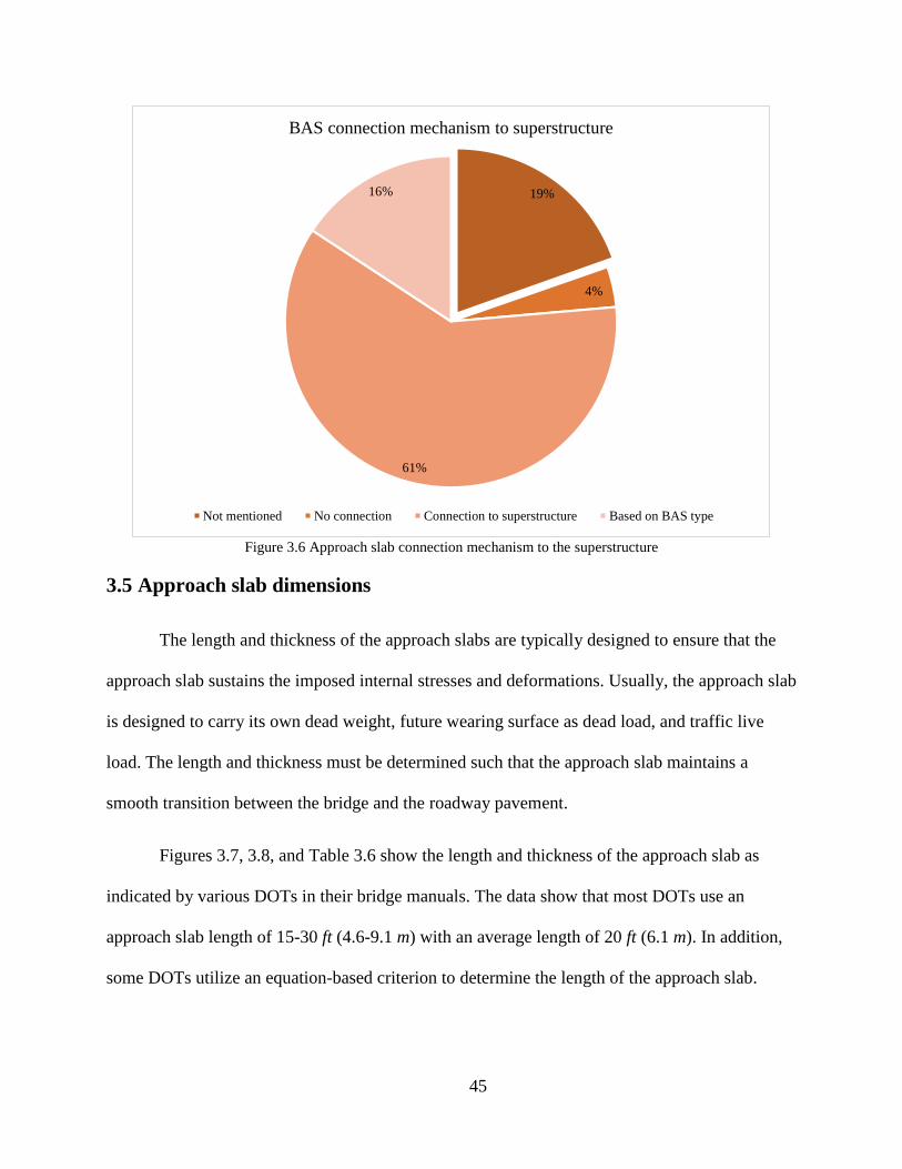
45
Figure 3.6 Approach slab connection mechanism to the superstructure
3.5 Approach slab dimensions
The length and thickness of the approach slabs are typically designed to ensure that the
approach slab sustains the imposed internal stresses and deformations. Usually, the approach slab
is designed to carry its own dead weight, future wearing surface as dead load, and traffic live
load. The length and thickness must be determined such that the approach slab maintains a
smooth transition between the bridge and the roadway pavement.
Figures 3.7, 3.8, and Table 3.6 show the length and thickness of the approach slab as
indicated by various DOTs in their bridge manuals. The data show that most DOTs use an
approach slab length of 15-30 ft (4.6-9.1 m) with an average length of 20 ft (6.1 m). In addition,
some DOTs utilize an equation-based criterion to determine the length of the approach slab.
19%
4%
61%
16%
BAS connection mechanism to superstructure
Not mentioned No connection Connection to superstructure Based on BAS type

46
These are shown in Table 3.5. The data also show that most DOTs use an approach slab
thickness of 9-15 in (229-381 mm) with an average thickness of 12 in (305 mm).
Table 3.5 Length of the approach slab using equation-based criterion
DOT Approach slab length Parameters
Colorado 20 sin 𝜃 θ = skew angle of the bridge
Nevada 2𝐷 D = structure depth
New York 1.5𝐻𝑎 Ha = abutment height
Ohio 1.5(𝐻 + 𝑤 + 1.5) cos 𝜃⁄
H = height of the embankment
w = width of the footing heel
θ = skew angle of the bridge

47
Figure 3.7 Approach slab length (ft)
Figure 3.8 Approach slab thickness (in)
22%
67%
9%2%
Approach slab length
10 - 15
15 - 25
25 - 35
˃ 35
62%
27%
11%
Approach slab thickness
8 - 12
12 - 15
15 - 18

48
Table 3.6 Approach slab dimensions
DOT Length (L) ft (m)
Thickness (T) in (mm) DOT
Length (L) ft (m)
Thickness (T) in (mm)
Arizona L ≥ 15 (4.6)
T = 12 (305) Montana —
Alaska — Nebraska L = 20 (6.1)
T = 14 (356)
Alabama L = 20 (6.1)
T ≥ 10 (254) Nevada[1]
L ≥ 24 (7.3)
T = 12 (305)
Arkansas L ≥ 16 (4.9)
T ≥ 9 (229) New Hampshire
L ≥ 10 (3)
T = 15 (381)
California L = 30 (9.1)
T = 12 (305) New Jersey
L ≥ 10 (3)
T = 18 (457)
Colorado[1] L ≥ 20 (6.1)
T = 12 (305) New Mexico
L ≥ 14 (4.3)
—
Connecticut L = 16 (4.9)
T = 15 (381) North Carolina
L ≥ 15 (4.6)
T ≥ 12 (305)
District of Columbia L ≥ 20 (6.1)
T = 15 (381) North Dakota
L = 20 (6.1)
T = 14 (356)
Delaware 18 (5.5) ≤ L ≤ 30 (9.1)
T = 16 (406) New York[1]
10 (3) ≥ L ≥ 25 (7.6)
T = 12 (305)
Florida L ≥ 30 (9.1)
T = 12 (305) Ohio[1]
L ≥ 15 (4.6)
12 (305) ≤ T ≤ 17 (432)
Georgia L ≥ 20 (6.1)
T = 10 (254) Oklahoma
L ≥ 20 (6.1)
T = 13 (330)
Hawaii — Oregon L ≥ 20 (6.1)
T ≥ 12 (305)
Idaho L = 20 (6.1)
T = 12 (305) Pennsylvania
L ≥ 25 (7.6)
T ≥ 16 (406)
Illinois L = 30 (9.1)
T = 15 (381) Rhode Island
L = 14 (4.3)
T = 14 (356)
Indiana L = 20 (6.1)
T ≥ 10 (254) South Carolina
L = 20 (6.1)
T = 12 (305)
Iowa L = 60 (18.3)
T = 10 (254) South Dakota
L = 20 (6.1)
T = 9 (229)
Kansas L = 33 (10.1)
T ≥ 10 (254) Tennessee
L = 24 (7.3)
T = 12 (305)
Kentucky L ≥ 20 (6.1)
T = 17 (432) Texas
L = 20 (6.1)
T = 13 (330)
Louisiana L ≥ 20 (6.1)
T ≥ 10 (254) Utah
L ≥ 25 (7.6)
—
Maine L = 15.5 (4.7)
T = 8 (203) Vermont
L ≥ 15 (4.6)
T ≥ 14 (356)
Maryland — Virginia L ≥ 20 (6.1)
T = 15 (381)
Massachusetts L ≥ 10 (3)
T = 10 (254) Washington
L ≥ 25 (7.6)
T = 13 (330)
Michigan L = 20 (6.1)
T = 12 (305) West Virginia
L ≥ 20 (6.1)
T = 12 (305)
Minnesota L = 20 (6.1)
T = 12 (305) Wisconsin
L = 20 (6.1)
T = 16 (406)
Mississippi — Wyoming L = 25 (7.6)
T = 10 (254)
Missouri L = 20 (6.1)
T = 12 (305)
[1] Utilizes equation-based criterion to determine the length of the approach slab (refer to Table 3.5)

49
3.6 Embankment and backfill considerations
Information regarding the type of the backfill material, slope of the backfill area,
compaction level of the backfill area, and the side slope of the embankment fill were retrieved
from the bridge manuals. The data (Table 3.7) show that the customary practice in the backfill
area is to utilize a free draining granular material backfill material with a slope of 1:1 (1 vertical
to 1 horizontal) and compacted to 95% of the standard proctor. The data also show that a slope of
1:2 (1 vertical to 2 horizontal) is commonly used on the sides of the embankment fills.
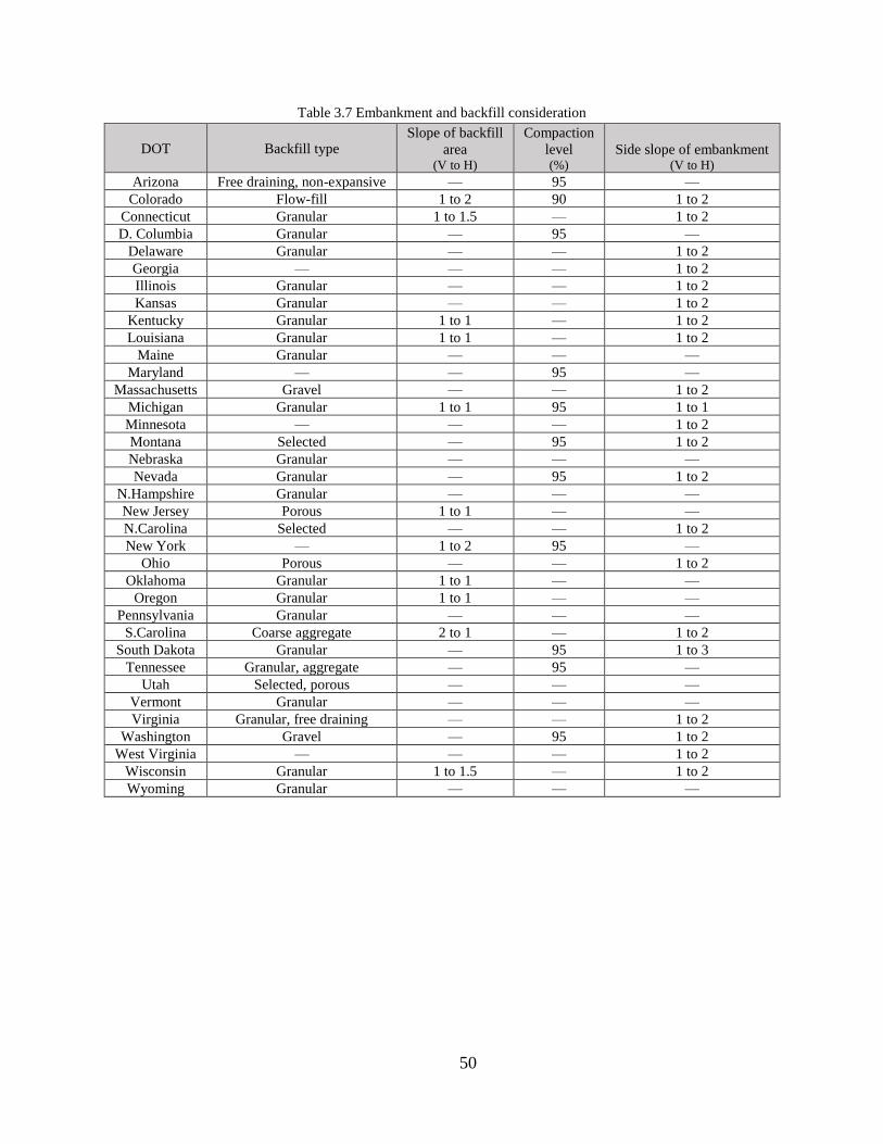
50
Table 3.7 Embankment and backfill consideration
DOT Backfill type Slope of backfill
area (V to H)
Compaction
level (%)
Side slope of embankment (V to H)
Arizona Free draining, non-expansive — 95 —
Colorado Flow-fill 1 to 2 90 1 to 2
Connecticut Granular 1 to 1.5 — 1 to 2
D. Columbia Granular — 95 —
Delaware Granular — — 1 to 2
Georgia — — — 1 to 2
Illinois Granular — — 1 to 2
Kansas Granular — — 1 to 2
Kentucky Granular 1 to 1 — 1 to 2
Louisiana Granular 1 to 1 — 1 to 2
Maine Granular — — —
Maryland — — 95 —
Massachusetts Gravel — — 1 to 2
Michigan Granular 1 to 1 95 1 to 1
Minnesota — — — 1 to 2
Montana Selected — 95 1 to 2
Nebraska Granular — — —
Nevada Granular — 95 1 to 2
N.Hampshire Granular — — —
New Jersey Porous 1 to 1 — —
N.Carolina Selected — — 1 to 2
New York — 1 to 2 95 —
Ohio Porous — — 1 to 2
Oklahoma Granular 1 to 1 — —
Oregon Granular 1 to 1 — —
Pennsylvania Granular — — —
S.Carolina Coarse aggregate 2 to 1 — 1 to 2
South Dakota Granular — 95 1 to 3
Tennessee Granular, aggregate — 95 —
Utah Selected, porous — — —
Vermont Granular — — —
Virginia Granular, free draining — — 1 to 2
Washington Gravel — 95 1 to 2
West Virginia — — — 1 to 2
Wisconsin Granular 1 to 1.5 — 1 to 2
Wyoming Granular — — —

51
CHAPTER 4 - DEVELOPMENT OF FINITE ELEMENT SOIL-
STRUCTURE INTERACTION MODEL
4.1 Introduction
The analytical modeling of any structure can be represented through a finite number of
elements that are computationally assembled and analyzed to obtain a solution for the structure.
For the purpose of this study, the commercial finite element software ABAQUS was used to run
the developed model that was constructed to analyze the soil-structure interaction effects.
In this study, three finite element models were developed, and parametric studies were
performed to evaluate the soil/approach slab settlement behind bridge abutments for various soil
conditions (Chapter 5), and to quantify the pile head settlement and load distribution along piles
as a function of pile-soil parameters (Chapter 6). Table 4.1 shows general description of the
employed models.
Table 4.1 Description of the simulation used in this study
Finite element model type Objective Examined parameter
Two-Dimensional Transverse
(Figure 4.1)
Simulate the soil settlement
behind bridge abutments.
Height of embankment fill
Embankment soil type
Side slope of embankment fill
Height of natural soil
Natural soil type
Two-Dimensional Longitudinal
(Figure 4.2)
Simulate the formation of the
bump at the end of the bridge.
Erosion of backfill material
Slope of backfill area
Backfill soil compaction level
Abutment type
Three-Dimensional Pile-Soil System
(Figure 4.3)
Simulate the behavior of piles
founded on various pile-soil
conditions.
Length of approach slab segment
Number of approach slab segments
Pile size (diameter)
Pile length
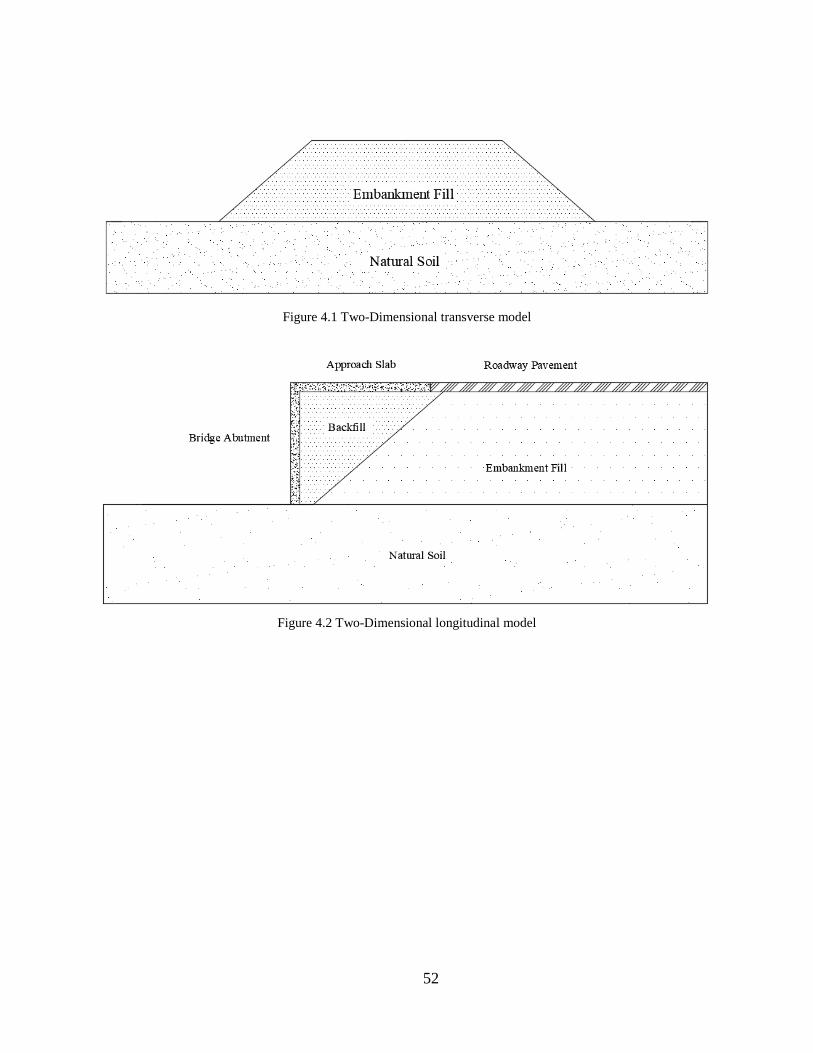
52
Figure 4.1 Two-Dimensional transverse model
Figure 4.2 Two-Dimensional longitudinal model
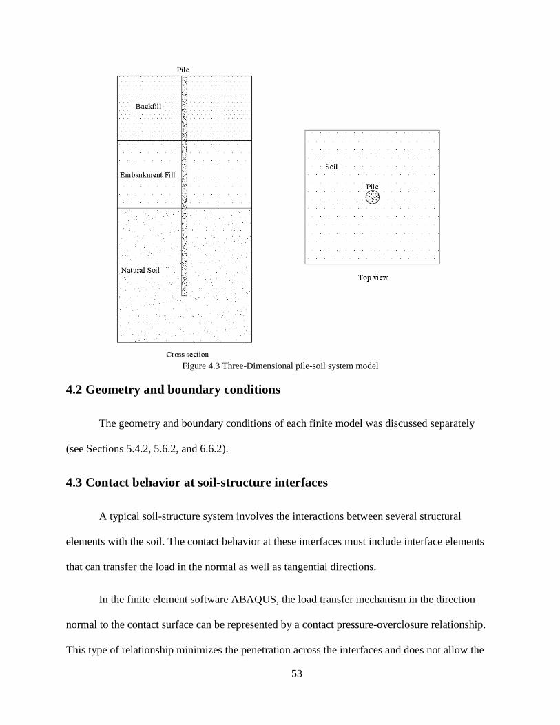
53
Figure 4.3 Three-Dimensional pile-soil system model
4.2 Geometry and boundary conditions
The geometry and boundary conditions of each finite model was discussed separately
(see Sections 5.4.2, 5.6.2, and 6.6.2).
4.3 Contact behavior at soil-structure interfaces
A typical soil-structure system involves the interactions between several structural
elements with the soil. The contact behavior at these interfaces must include interface elements
that can transfer the load in the normal as well as tangential directions.
In the finite element software ABAQUS, the load transfer mechanism in the direction
normal to the contact surface can be represented by a contact pressure-overclosure relationship.
This type of relationship minimizes the penetration across the interfaces and does not allow the
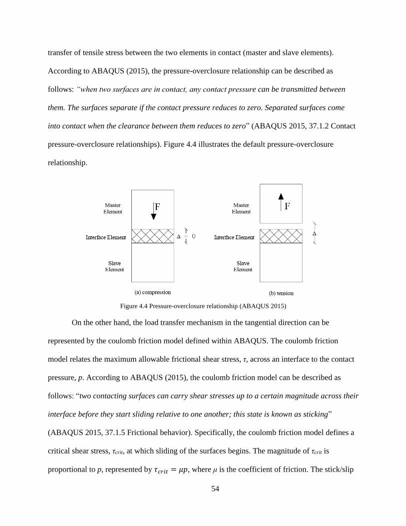
54
transfer of tensile stress between the two elements in contact (master and slave elements).
According to ABAQUS (2015), the pressure-overclosure relationship can be described as
follows: “when two surfaces are in contact, any contact pressure can be transmitted between
them. The surfaces separate if the contact pressure reduces to zero. Separated surfaces come
into contact when the clearance between them reduces to zero” (ABAQUS 2015, 37.1.2 Contact
pressure-overclosure relationships). Figure 4.4 illustrates the default pressure-overclosure
relationship.
Figure 4.4 Pressure-overclosure relationship (ABAQUS 2015)
On the other hand, the load transfer mechanism in the tangential direction can be
represented by the coulomb friction model defined within ABAQUS. The coulomb friction
model relates the maximum allowable frictional shear stress, τ, across an interface to the contact
pressure, p. According to ABAQUS (2015), the coulomb friction model can be described as
follows: “two contacting surfaces can carry shear stresses up to a certain magnitude across their
interface before they start sliding relative to one another; this state is known as sticking”
(ABAQUS 2015, 37.1.5 Frictional behavior). Specifically, the coulomb friction model defines a
critical shear stress, τcrit, at which sliding of the surfaces begins. The magnitude of τcrit is
proportional to p, represented by 𝜏𝑐𝑟𝑖𝑡 = 𝜇𝑝, where μ is the coefficient of friction. The stick/slip

55
calculations within ABAQUS determine when a point transitions from sticking to slipping or
from slipping to sticking based upon the value of τ (ABAQUS 2015). Figure 4.5 illustrates the
slipping behavior of the coulomb friction model.
Figure 4.5 Slipping behavior of the coulomb friction model (ABAQUS 2015)
ABAQUS (2015) provides general rules to assign the master and slave elements to the
modeled component. Accordingly, master elements should be assigned to those parts that are
larger, stiffer and have coarser mesh.
4.4 Analysis procedures
The analysis procedures of each finite model was discussed separately (see Sections
5.4.3, 5.6.4, and 6.6.4).
4.5 Simulating non-linear behavior of soil
When soil is subjected to load, it undergoes elastic and plastic strain. Elastic strain is
reversible while plastic strain is irreversible and causes permanent deformation in the material.
Elasticity theory, namely Hooke’s law, is typically used to describe the reversible deformation of
the material, while plasticity theory is used to describe the irreversible behavior of the material.

56
Ultimately, the total strain (ɛ) is decomposed into an elastic strain component (ɛe) and plastic
strain component (ɛp).
Soil constitutive models, such as the Modified Drucker-Prager/Cap model and Modified
Cam-Clay model, are typically designed to include both elastic and plastic behavior of the soil
under various types of loading. These constitutive models are developed based on experimental
results, typically triaxial shear and isotropic consolidation tests.
4.5.1 Modified Drucker-Prager/Cap constitutive model (MDPCM)
The MDPCM is widely used in finite element analyses to model the behavior of soils and
rocks. It is designed such that it can fit the Mohr-Coulomb shear failure surface with an
additional cap surface. The cap provides a plastic hardening mechanism and helps control
volume dilatancy of the material (ABAQUS 2015). The yield surface of the MDPCM consists of
three segments: shear failure surface segment, Fs, compression cap segment, Fc, and transition
segment in which connects Fs with Fc (Figures 4.6 and 4.7).
Figure 4.6 Drucker-Prager/Cap failure surface (ABAQUS 2015)

57
Figure 4.7 Yield/flow surface in the deviatoric plane (ABAQUS 2015)
The shear failure surface, Fs, is defined in terms of the modified cohesion, d, and
modified angle of internal friction, β, and is given by
𝐹𝑠 = 𝑡 − 𝑝 tan 𝛽 − 𝑑 = 0 4-1
Where
p = Equivalent pressure stress = −1
3𝑡𝑟𝑎𝑐𝑒(𝜎) = −
1
3(𝜎1 + 𝜎2 + 𝜎3)
t = Deviatoric stress measure = 𝑞
2[1 +
1
𝐾− (1 −
1
𝐾) (
𝑟
𝑞)
3
]
q = Mises equivalent stress = Shear stress = √1
2[(𝜎1 − 𝜎2)2 + (𝜎2 − 𝜎3)2 + (𝜎1 − 𝜎3)2]
K = Parameter that controls the shape of the yield surface on the deviatoric plane,
typically 0.778 ≤ K ≤ 1.0 (see Figure 4.7).
r = Third stress invariant.
The cap failure surface, Fc, and transition surface, Ft, are given as

58
𝐹𝑐 = √(𝑝 − 𝑝𝑎)2 + (𝑅𝑡
1 + 𝛼 −𝛼
cos 𝛽
)
2
− 𝑅(𝑑 + 𝑝𝑎 tan 𝛽) = 0 4-2
𝐹𝑡 = √(𝑝 − 𝑝𝑎)2 + [𝑡 − (1 −𝛼
cos 𝛽) (𝑑 + 𝑝𝑎 tan 𝛽)]
2
− 𝛼(𝑑 + 𝑝𝑎 tan 𝛽) = 0 4-3
Where
R = Eccentricity parameter that controls the shape of the cap surface.
α = Parameter that shape of define the transition yield surface, typically 0.01 ≤ α ≤ 0.05.
pa = Parameter that controls the hardening/softening behavior as a function of volumetric
plastic strain = 𝑝𝑏+𝑅𝑑
1+𝑅 tan 𝛽
pb = Hydrostatic yield stress (user-defined).
The plastic flow (Figure 4.8) is defined by a non-associated segment on the shear failure
and transition region, Gs, and an associated segment on the cap region, Gc, given as
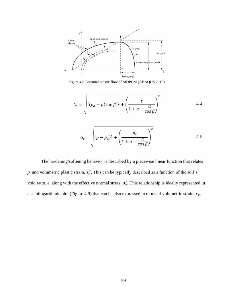
59
Figure 4.8 Potential plastic flow of MDPCM (ABAQUS 2015)
𝐺𝑠 = √[(𝑝𝑎 − 𝑝) tan 𝛽]2 + (𝑡
1 + 𝛼 −𝛼
cos 𝛽
)
2
4-4
𝐺𝑐 = √(𝑝 − 𝑝𝑎)2 + (𝑅𝑡
1 + 𝛼 −𝛼
cos 𝛽
)
2
4-5
The hardening/softening behavior is described by a piecewise linear function that relates
pb and volumetric plastic strain, 𝜀𝑣𝑝. This can be typically described as a function of the soil’s
void ratio, e, along with the effective normal stress, 𝜎𝑣′ . This relationship is ideally represented in
a semilogarithmic plot (Figure 4.9) that can be also expressed in terms of volumetric strain, 𝜀𝑣.

60
Figure 4.9 Typical consolidation curves (Coduto 2001)
The above figure shows that e and 𝜀𝑣 are indirectly related to 𝜎𝑣′ during the loading and
unloading curves represented by the compression and swelling indexes, Cc and Cs, respectively.
From this relationship, the volumetric plastic strain can be derived as (Helwany 2007)
𝜀𝑣𝑜𝑙
𝑝𝑙 =𝐶𝑐 − 𝐶𝑠
(ln 10)(1 + 𝑒0)ln
𝜎′
𝜎𝑐′ 4-6
4.5.2 Modified Cam-Clay model (MCCM)
The MCCM is critical state criterion that is used to describe the behavior of fully
saturated clay soils. The soil reaches the critical state after passing through series states of
yielding resulting in strain hardening or softening. At that stage, change in soil volume occurs
with no additional shear stress (Zaman, Gioda and Booker 2000).
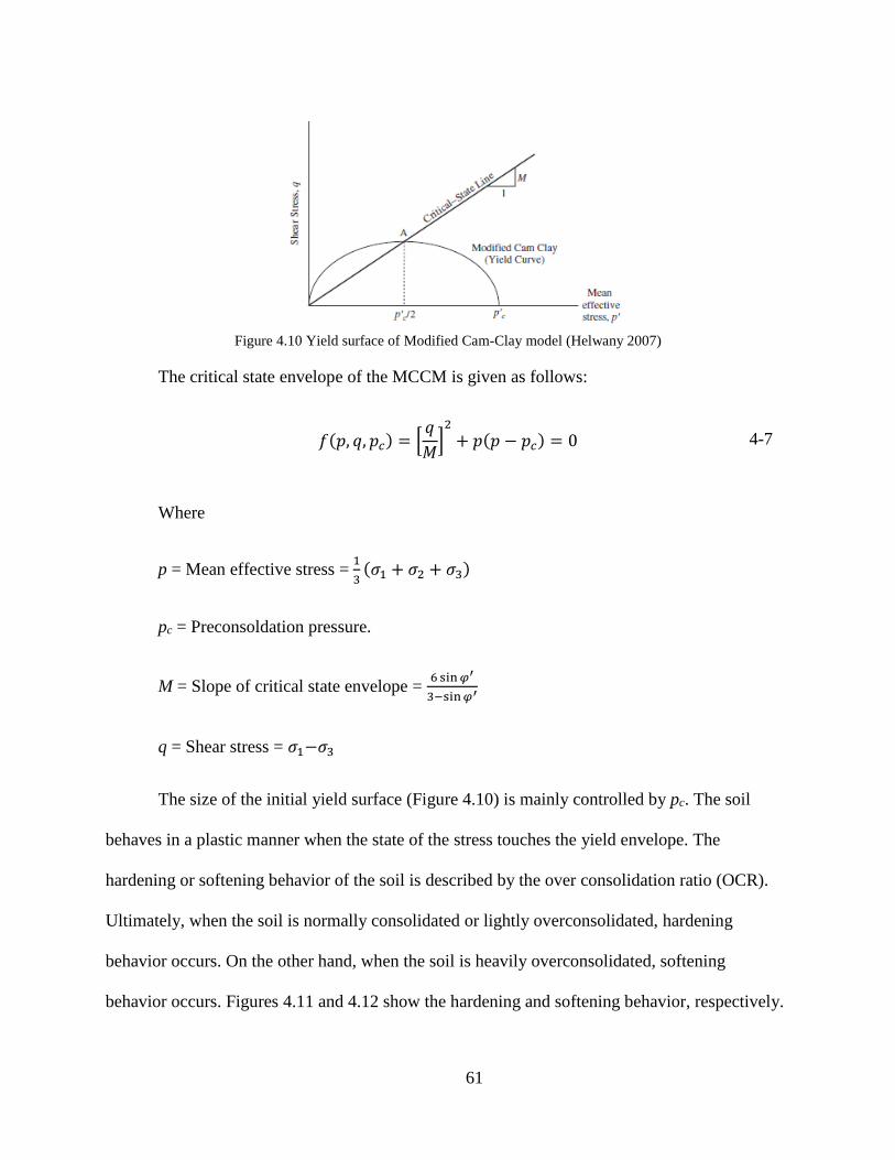
61
Figure 4.10 Yield surface of Modified Cam-Clay model (Helwany 2007)
The critical state envelope of the MCCM is given as follows:
𝑓(𝑝, 𝑞, 𝑝𝑐) = [
𝑞
𝑀]
2
+ 𝑝(𝑝 − 𝑝𝑐) = 0 4-7
Where
p = Mean effective stress = 1
3(𝜎1 + 𝜎2 + 𝜎3)
pc = Preconsoldation pressure.
M = Slope of critical state envelope = 6 sin 𝜑′
3−sin 𝜑′
q = Shear stress = 𝜎1−𝜎3
The size of the initial yield surface (Figure 4.10) is mainly controlled by pc. The soil
behaves in a plastic manner when the state of the stress touches the yield envelope. The
hardening or softening behavior of the soil is described by the over consolidation ratio (OCR).
Ultimately, when the soil is normally consolidated or lightly overconsolidated, hardening
behavior occurs. On the other hand, when the soil is heavily overconsolidated, softening
behavior occurs. Figures 4.11 and 4.12 show the hardening and softening behavior, respectively.

62
Figure 4.11 Hardening behavior of the MCCM (Zaman, Gioda and Booker 2000)
Figure 4.12 Softening behavior of the MCCM (Zaman, Gioda and Booker 2000)
The elastic behavior can be described by bulk modulus, K. The change in the bulk
stiffness for loading and unloading is represented by
Loading �̇� = −𝑝
𝜆𝜀�̇� = 𝐾𝜀�̇� 4-8
Unloading �̇� = −𝑝
𝜅𝜀�̇� = 𝐾𝜀�̇� 4-9
Where 𝜅 and 𝜆 are modified compression index and modified swelling index,
respectively.

63
4.6 Material properties
The concrete in the structural components, i.e. abutment wall, approach slab, pile and
roadway pavement, was assumed to be behave in a linearly elastic manner with a modulus of
elasticity that is consistent with a design compressive strength of 4000 psi (28 MPa). Table 4.2
shows the concrete material parameters assumed for the abutment wall, approach slab, pile and
roadway pavement.
Table 4.2 Material parameters used for the structural components
Parameter Concrete
Density (γ) pcf (kN/m3) 150 (24)
Modulus of elasticity (E) ksi (MPa) 3,605 (24,856)
Poisson’s ratio (ѵ) 0.21
The soil properties play a significant role in the settlement analysis. These properties are
typically collected from fundamental soil tests such as the triaxial and consolidation tests. In this
study, a wide range of soil properties were adopted from test results reported by other researchers
representing a variety of soil conditions from across the United States.
Three different zones were considered in the analysis; the natural soil, the embankment
fill, and the backfill soil. For the purpose of this study, the backfill soil was selected to be sand,
which was classified based on the degree of the compaction (i.e. 95% or 90%). The natural and
embankment soils were considered to be clay and were classified based on the degree of
compressibility (i.e. highly compressible, moderately compressible, or low compressible).
According to Coduto (2001), the degree of compressibility of soils can be determined based on a
parameter that is related to the compression index, Cc, and the initial void ratio, e0. The soil is
considered low compressible (LC) when (𝐶𝑐
1+𝑒0) falls between 0.0 to 0.10, moderately

64
compressible (MC) when (𝐶𝑐
1+𝑒0) falls between 0.10 to 0.20, and highly compressible (HC) when
𝐶𝑐
1+𝑒0 is greater than 0.20.
Additionally, empirical relationships and typical values were used to obtain the soil
parameters needed for the settlement analysis when actual test results for these parameters were
not reported. Some of the empirical relationships used are listed below (B. M. Das 2011)
• Initial void ratio (e0):
𝑒0 =
𝐶𝑐
1.15+ 0.35 4-10
• Swelling index (Cs):
𝐶𝑠 = 0.1𝐶𝑐 4-11
• Specific gravity of clay soil (Gs):
𝐺𝑠 = 2.70 → 2.90 4-12
• Water content (w):
𝛾 =
(1 + 𝑤)𝐺𝑠𝛾𝑤
1 + 𝑒0 4-13
• Coefficient of permeability (k):
𝑘 = 𝑚𝑣 × 𝛾𝑤 × 𝐶𝑣 4-14
Where:
Cv = Coefficient of consolidation = 10−1.2697 ln(𝐿𝐿)+2.1515
LL =Liquid limit.
mv = Volume coefficient of compressibility = ∆𝑒/[∆𝜎′(1 + 𝑒𝑎𝑣)]
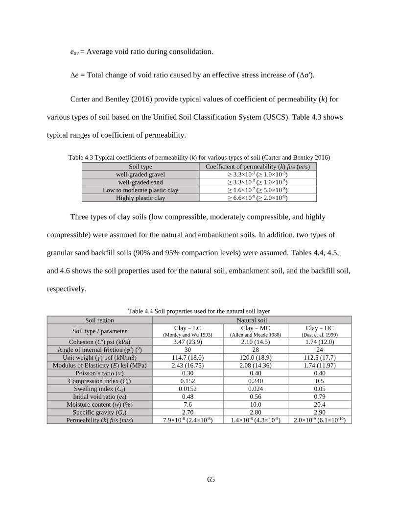
65
eav = Average void ratio during consolidation.
∆e = Total change of void ratio caused by an effective stress increase of (Δσ').
Carter and Bentley (2016) provide typical values of coefficient of permeability (k) for
various types of soil based on the Unified Soil Classification System (USCS). Table 4.3 shows
typical ranges of coefficient of permeability.
Table 4.3 Typical coefficients of permeability (k) for various types of soil (Carter and Bentley 2016)
Soil type Coefficient of permeability (k) ft/s (m/s)
well-graded gravel ≥ 3.3×10⁻³ (≥ 1.0×10⁻³)
well-graded sand ≥ 3.3×10⁻⁵ (≥ 1.0×10⁻⁵)
Low to moderate plastic clay ≥ 1.6×10⁻⁷ (≥ 5.0×10⁻⁸)
Highly plastic clay ≥ 6.6×10⁻⁹ (≥ 2.0×10⁻⁹)
Three types of clay soils (low compressible, moderately compressible, and highly
compressible) were assumed for the natural and embankment soils. In addition, two types of
granular sand backfill soils (90% and 95% compaction levels) were assumed. Tables 4.4, 4.5,
and 4.6 shows the soil properties used for the natural soil, embankment soil, and the backfill soil,
respectively.
Table 4.4 Soil properties used for the natural soil layer
Soil region Natural soil
Soil type / parameter Clay – LC
(Monley and Wu 1993) Clay – MC
(Allen and Meade 1988) Clay – HC
(Das, et al. 1999)
Cohesion (C') psi (kPa) 3.47 (23.9) 2.10 (14.5) 1.74 (12.0)
Angle of internal friction (φ') (0) 30 28 24
Unit weight (ɣ) pcf (kN/m3) 114.7 (18.0) 120.0 (18.9) 112.5 (17.7)
Modulus of Elasticity (E) ksi (MPa) 2.43 (16.75) 2.08 (14.36) 1.74 (11.97)
Poisson’s ratio (ѵ) 0.30 0.40 0.40
Compression index (Cc) 0.152 0.240 0.5
Swelling index (Cs) 0.0152 0.024 0.05
Initial void ratio (e0) 0.48 0.56 0.79
Moisture content (w) (%) 7.6 10.0 20.4
Specific gravity (Gs) 2.70 2.80 2.90
Permeability (k) ft/s (m/s) 7.9×10⁻⁸ (2.4×10⁻⁸) 1.4×10⁻⁸ (4.3×10⁻⁹) 2.0×10⁻⁹ (6.1×10⁻¹⁰)

66
Table 4.5 Soil properties used for the embankment fill layer
Soil region Embankment fill
Soil type / parameter Clay – LC
(Laguros, et al. 1991) Clay – MC
(Laguros, et al. 1991) Clay – HC
(Allen and Meade 1988)
Cohesion (C') psi (kPa) 3.50 (24.1) 1.20 (8.3) 0.5 (3.4)
Angle of internal friction (φ') (0) 34 30 29
Unit weight (ɣ) pcf (kN/m3) 122.0 (19.2) 127 (20.0) 130 (20.4)
Modulus of Elasticity (E) ksi (MPa) 1.56 (10.77) 1.39 (9.58) 1.22 (8.38)
Poisson’s ratio (ѵ) 0.30 0.40 0.40
Compression index (Cc) 0.087 0.30 0.42
Swelling index (Cs) 0.014 0.03 0.042
Initial void ratio (e0) 0.43 0.61 0.72
Moisture content (w) (%) 3.5 12.8 19.4
Specific gravity (Gs) 2.70 2.80 2.90
Permeability (k) ft/s (m/s) 2.8×10⁻⁷ (8.53×10⁻⁸) 7.3×10⁻⁸ (2.2×10⁻⁸) 8.9×10⁻⁹ (2.7×10⁻⁹)
Table 4.6 Soil properties used for the backfill soil layer
Soil Region Backfill soil
Soil type / parameter Sand - 95%
(McGrath, et al. 2002) Sand - 90%
(McGrath, et al. 2002)
Cohesion (C') psi (kPa) 0.0 0.0
Angle of internal friction (φ') (0) 43 38
Unit weight (ɣ) pcf (kN/m3) 128.0 (20.1) 126 (19.8)
Modulus of Elasticity (E) ksi (MPa) 2.90 (20.0) 1.90 (13.1)
Poisson’s ratio (ѵ) 0.30 0.30
Initial void ratio (e0) 0.50 0.68
Permeability (k) ft/s (m/s) 1.0×10⁻³ (3.0×10⁻⁴) 2.2×10⁻³ (6.7×10⁻⁴)
The modified Drucker-Prager/Cap material model was used to describe the soil behavior
in the computer models. The input parameters needed in the finite element analysis to model the
soil were obtained such that they would match the properties provided in the above tables. Table
4.7 shows the input parameters used to model the soil.
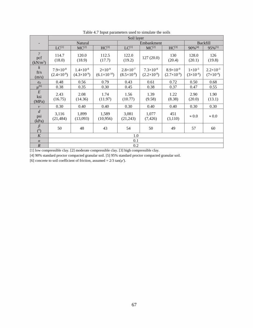
67
Table 4.7 Input parameters used to simulate the soils
-
Soil layer
Natural Embankment Backfill
LC[1] MC[2] HC[3] LC[1] MC[2] HC[3] 90%[4] 95%[5]
γ
pcf
(kN/m3)
114.7
(18.0)
120.0
(18.9)
112.5
(17.7)
122.0
(19.2) 127 (20.0)
130
(20.4)
128.0
(20.1)
126
(19.8)
k
ft/s
(m/s)
7.9×10⁻⁸
(2.4×10⁻⁸)
1.4×10⁻⁸
(4.3×10⁻⁹)
2×10⁻⁹
(6.1×10⁻¹⁰)
2.8×10⁻⁷
(8.5×10⁻⁸)
7.3×10⁻⁸
(2.2×10⁻⁸)
8.9×10⁻⁹
(2.7×10⁻⁹)
1×10⁻³
(3×10⁻⁴)
2.2×10⁻³
(7×10⁻⁴)
e0 0.48 0.56 0.79 0.43 0.61 0.72 0.50 0.68
μ[6] 0.38 0.35 0.30 0.45 0.38 0.37 0.47 0.55
E
ksi
(MPa)
2.43
(16.75)
2.08
(14.36)
1.74
(11.97)
1.56
(10.77)
1.39
(9.58)
1.22
(8.38)
2.90
(20.0)
1.90
(13.1)
ѵ 0.30 0.40 0.40 0.30 0.40 0.40 0.30 0.30
d
psi
(kPa)
3,116
(21,484)
1,899
(13,093)
1,589
(10,956)
3,081
(21,243)
1,077
(7,426)
451
(3,110) ≈ 0.0 ≈ 0.0
β
(0) 50 48 43 54 50 49 57 60
K 1.0
α 0.1
R 0.2 [1] low compressible clay. [2] moderate compressible clay. [3] high compressible clay.
[4] 90% standard proctor compacted granular soil. [5] 95% standard proctor compacted granular soil.
[6] concrete to soil coefficient of friction, assumed = 2/3 tan(φ').

68
CHAPTER 5 - SIMULATION OF SOIL SETTLEMENT BEHIND
BRIDGE ABUTMENTS
5.1 Chapter background
The bridge approach slab is part of a transition system in which the end of the bridge is
connected to the roadway pavement (Figure 5.1). Its function is to carry traffic loads and provide
drivers with a smooth ride as their vehicle travels from the roadway to the bridge and vice versa
(Abu-Farsakh and Chen 2014).
Figure 5.1 Typical longitudinal cross section of a bridge
Due to excessive long-term settlement of soil under the bridge approach slab, a bump can
typically develop at the end of the bridge. The bump at the end of the bridge is a well-known
problem that affects about 25% of the bridges in the United States, resulting in an estimated $100
million per year in maintenance expenditures (Briaud, James and Hoffman 1997). The bump at
the end of the bridge can lead to unsafe driving conditions, vehicle damage, and additional
69
maintenance cost. Furthermore, distress, fatigue, and deterioration of the bridge deck and
expansion joint are possible consequences of such a problem (Briaud, James and Hoffman 1997,
Hu, et al. 1979, Nicks 2015).
Thus, an accurate prediction of the ultimate soil deflection profile behind the bridge
abutment is an important parameter in the proper design of the approach slab, and for the
mitigation of the bump at the end of the bridge. Terzaghi’s theories of consolidation are widely
used in many geotechnical engineering applications including estimations of settlement of fine-
grained soils. The one-dimensional consolidation theory is not always effective in predicting the
settlement profile behind bridge abutments (Helwany 2007).
5.2 Chapter problem statement
The longitudinal soil deflection profile behind bridge abutment is rather difficult to
predict using a closed-form solution. The difficulty arises due to the nature of the problem (i.e.
two- or three-dimensional problem) as well as the number of factors involved. Some of these
factors include the variation in the soil profile, the interaction between the abutment wall and the
adjacent backfill soil, the size of the backfill area, and the sequential construction of the
embankment fill, approach slab and the roadway pavement.
Typically, the soil profile would consist of several soil layers, with some layers
deforming in a time-dependent manner, due to primary and secondary settlements. Additionally,
the friction developed between the abutment wall and the adjacent soil (backfill soil) restricts
some of the soil movement in the vicinity of the abutment wall, while the soil away from the
wall would not be similarly affected and would therefore have larger settlement. This type of
behavior would typically result in a curved soil settlement profile behind the bridge abutment.
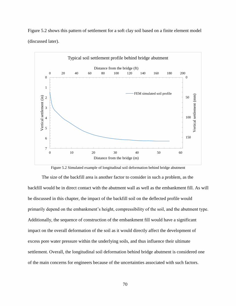
70
Figure 5.2 shows this pattern of settlement for a soft clay soil based on a finite element model
(discussed later).
Figure 5.2 Simulated example of longitudinal soil deformation behind bridge abutment
The size of the backfill area is another factor to consider in such a problem, as the
backfill would be in direct contact with the abutment wall as well as the embankment fill. As will
be discussed in this chapter, the impact of the backfill soil on the deflected profile would
primarily depend on the embankment’s height, compressibility of the soil, and the abutment type.
Additionally, the sequence of construction of the embankment fill would have a significant
impact on the overall deformation of the soil as it would directly affect the development of
excess pore water pressure within the underlying soils, and thus influence their ultimate
settlement. Overall, the longitudinal soil deformation behind bridge abutment is considered one
of the main concerns for engineers because of the uncertainties associated with such factors.
0 10 20 30 40 50 60
0
50
100
150
0
1
2
3
4
5
6
7
0 20 40 60 80 100 120 140 160 180 200
Distance from the bridge (m)
Ver
tica
l se
ttle
men
t (m
m)
Ver
tica
l se
ttle
men
t (i
n)
Distance from the bridge (ft)
Typical soil settlement profile behind bridge abutment
FEM simulated soil profile

71
Finite element methods are widely used to solve engineering problems, including
estimating long-term soil settlement. The advantage of this analytical approach can simulate full-
scale conditions with a various range of parameters. Therefore, it can serve as a practical tool in
predicting the longitudinal soil settlement profile behind bridge abutment.
5.3 Chapter objectives
The objective of this phase of the study is to develop empirical relationships that can be
used to evaluate the ultimate soil settlement profile along a longitudinal line behind the bridge
abutment. Such equations would be beneficial in making reliable predictions of the long-term
differential settlement of the approach slab, and to plan its design. The empirical equations are
derived by conducting a parametric study using a finite element model that includes the effects
of various parameters on the soil deflection profile.
5.4 Development and verification of transverse soil finite element model
5.4.1 Introduction
In this phase of the study, a two-dimensional transverse model was generated to perform
long-term soil settlement analysis. In this simulation, the embankment fill is to be constructed on
top of the natural soil layer. The objective of this analysis was to quantify the surface
deformation of the soil in a location that is away from the bridge abutment. The outcome of this
simulation can be used to roughly estimate the resulting differential settlement the approach slab
founded on similar soil conditions. Figure 5.3 shows the general layout of the two-dimensional
transverse model.

72
Figure 5.3 Layout of the two-dimensional transverse model
5.4.2 Geometry and boundary conditions
An important aspect of the soil finite element model is selecting the location and types of
boundary conditions (i.e. displacement and/or pore pressure boundary conditions) in an efficient
and effective manner.
The bottom of the model would represent a location where no soil movement occurs.
This location can be determined using the standard penetration test (typically provided in the
borehole log profile) whereas a high value indicates a hard layer, such as bedrock. At this
location, both vertical and horizontal movements are restricted (assumed to be zero). In addition,
no water seepage would be expected to occur at this location, thus, impervious boundary was
assumed. The top surfaces of the soil were free to move in all directions. Furthermore, water
would be expected to flow through the top surfaces, thus, pervious boundary was assumed.
The soil mass must be sufficiently extended in the transverse direction to capture the
behavior of the soil. Laguros et al. (1991) recommend extending the natural soil mass a distance
of at least 2 (De + Dse), where De is the base width of the embankment fill and Dse is the base
width of the sloped part of the embankment fill. Figure 5.4 shows the geometry and boundary
conditions used in this analysis.

73
Figure 5.4 Boundary condition of the Two-Dimensional transverse model
In the above figure,
He = height of the embankment fill.
Sse = side slope of the embankment fill.
Hn = height of the natural soil layer.
Dn = base width of the natural soil.
In this study, He, De, Sse, Hn and Dn were varied according to the parametric study matrix
found in Table 5.5.
5.4.3 Analysis procedures for transverse soil model
In soil settlement analysis, timing is a very important factor that influences the soil
behavior. This was taken into consideration during the simulation in which the construction of
the embankment fill was implemented in a sequential manner. Hopkins (1985) provides an
empirical equation to estimate the rate of the loading of embankment fill, Tc, in days, based on its
height, He, in feet, as follows:

74
𝑇𝑐 = 10(1.2376 log 𝐻𝑒+0.1122) 5-1
Accordingly, the analysis procedures used to run the transverse soil model included the
following steps:
1- Applying a geostatic load on the natural soil layer. In this step, the effective self-
weight of the natural soil was applied. The geostatic step assures that equilibrium
is satisfied within the natural soil layer, and that the initial stress condition in all
elements falls within the initial yield surface.
2- Constructing the embankment fill over a period of time. In this step, the effective
self-weight of the embankment soil was applied. This was done in a coupled
(consolidation) step where the load of the embankment is applied in a timely
manner using equation 5-1.
3- Consolidation step/steps. In this step/steps, the calculations of the primary
settlement (consolidation process) and secondary settlement (creep) were made.
5.4.4 Material properties
The Modified Drucker-Prager/Cap material model was used to simulate the behavior of
the soils. Table 4.7 shows the input parameters used to model the soil.
5.4.5 Verification analysis
In this part of the study, a finite element model was generated to simulate the long-term
soil behavior. The objective was to compare the simulated ultimate soil settlement with
analytical solution (one-dimensional Terzaghi’s theory) as well as an actual bridge-site (two-
dimensional analysis).

75
5.4.5.1 One-dimensional analysis
In this part of the analysis, the simulation of the soil behavior using the Modified Cam-
Clay model and Modified Drucker-Prager/Cap model were compared against the Terzaghi’s one-
dimensional consolidation solution. This comparison was helpful in selecting the material model
that fits the provided data in which allows for an accurate calibration of the material parameters.
Terzaghi’s one-dimensional consolidation theory assumes that water flow and
deformation of the soil occurs in one direction only, i.e. the vertical direction, and ignores any
lateral deformation of the soil. It gives an estimated solution for the settlement of a fully
saturated clay layer having a thickness, Hc, and subjected to a uniform pressure, 𝛥𝜎. The ultimate
settlement, Sc, for a normally consolidated clay is given as follows: (B. M. Das 2011)
𝑆𝑐 =
𝐻𝑐𝐶𝑐
1 + 𝑒0log
𝜎0′ + 𝛥𝜎′
𝜎0′ 5-2
Where
Cc = Compression index.
Cs = Swelling index.
e0 = Initial void ratio.
𝜎0′ = Average effective vertical stress.
In order to simulate similar behavior of Terzaghi’s one-dimensional solution, a normally
consolidated fully saturated clay layer was considered in this analysis. The clay layer was
assumed to be located between two sand layers (Figure 5.5). A uniform pressure of 𝛥𝜎 = 2100
psf (100 kPa) was to be applied on the top of the sand layer.

76
Figure 5.5 Geometry of the settlement problem
For this analysis, a one-dimensional finite element model was generated. A strip along
the vertical direction was modeled, Wsoil = 1 ft (0.3 m). In addition, one-half of the geometry,
across the horizontal axis, was modeled. Along the vertical sides, the soil was assumed to move
in the vertical direction only. Figure 5.6 shows the boundary conditions used in the analysis.

77
Figure 5.6 Boundary condition of the settlement problem
In the above figures,
Hs = height of the sand layer.
Hc = height of the clay layer.
In this analysis, Hs and Hc were taken as 20 ft (6.1 m), and 3 ft (1.0 m), respectively. The
input parameters used to simulate the soils are shown in Table 5.1. Figure 5.7 shows the finite
element discretization.
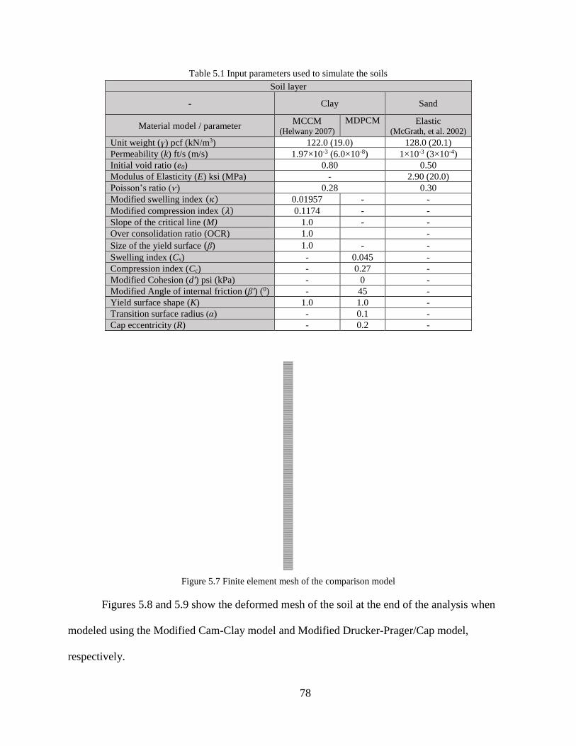
78
Table 5.1 Input parameters used to simulate the soils
Soil layer
- Clay Sand
Material model / parameter MCCM
(Helwany 2007) MDPCM
Elastic
(McGrath, et al. 2002)
Unit weight (ɣ) pcf (kN/m3) 122.0 (19.0) 128.0 (20.1)
Permeability (k) ft/s (m/s) 1.97×10⁻³ (6.0×10⁻⁸) 1×10⁻³ (3×10⁻⁴)
Initial void ratio (e0) 0.80 0.50
Modulus of Elasticity (E) ksi (MPa) - 2.90 (20.0)
Poisson’s ratio (ѵ) 0.28 0.30
Modified swelling index (𝜅) 0.01957 - -
Modified compression index (𝜆) 0.1174 - -
Slope of the critical line (M) 1.0 - -
Over consolidation ratio (OCR) 1.0 -
Size of the yield surface (β) 1.0 - -
Swelling index (Cs) - 0.045 -
Compression index (Cc) - 0.27 -
Modified Cohesion (d') psi (kPa) - 0 -
Modified Angle of internal friction (β') (0) - 45 -
Yield surface shape (K) 1.0 1.0 -
Transition surface radius (α) - 0.1 -
Cap eccentricity (R) - 0.2 -
Figure 5.7 Finite element mesh of the comparison model
Figures 5.8 and 5.9 show the deformed mesh of the soil at the end of the analysis when
modeled using the Modified Cam-Clay model and Modified Drucker-Prager/Cap model,
respectively.

79
Figure 5.8 Vertical deformation contour at the end of the analysis (MCCM) (ft)
Figure 5.9 Deformed mesh at the end of the analysis (MDPCM) (ft)
Figure 5.22 shows the simulated settlement history of the clay layer. The figure shows
that the Modified Cam-Clay model and Modified Drucker-Prager/Cap model simulated the soil
settlement behavior reasonably well when compared with Terzaghi’s one-dimensional solution.
Hence, both material models can be used to describe the soil behavior using parameters values
shown in Table 5.1 (i.e. size of the yield surface, β, yield surface shape, K, transition surface
radius, α, and cap eccentricity, R).
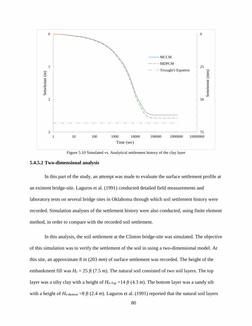
80
Figure 5.10 Simulated vs. Analytical settlement history of the clay layer
5.4.5.2 Two-dimensional analysis
In this part of the study, an attempt was made to evaluate the surface settlement profile at
an existent bridge-site. Laguros et al. (1991) conducted detailed field measurements and
laboratory tests on several bridge sites in Oklahoma through which soil settlement history were
recorded. Simulation analyses of the settlement history were also conducted, using finite element
method, in order to compare with the recorded soil settlement.
In this analysis, the soil settlement at the Clinton bridge-site was simulated. The objective
of this simulation was to verify the settlement of the soil in using a two-dimensional model. At
this site, an approximate 8 in (203 mm) of surface settlement was recorded. The height of the
embankment fill was He = 25 ft (7.5 m). The natural soil consisted of two soil layers. The top
layer was a silty clay with a height of Hn-Top =14 ft (4.3 m). The bottom layer was a sandy silt
with a height of Hn-Bottom =8 ft (2.4 m). Laguros et al. (1991) reported that the natural soil layers
0
25
50
75
0
1
2
3
1 10 100 1000 10000 100000 1000000 10000000
Set
tele
mnt
(mm
)
Set
tele
mnt
(in)
Time (sec)
MCCM
MDPCM
Terzaghi's Equation
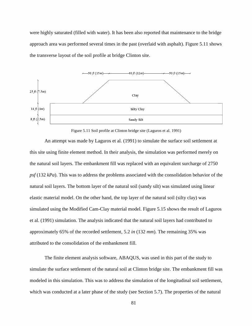
81
were highly saturated (filled with water). It has been also reported that maintenance to the bridge
approach area was performed several times in the past (overlaid with asphalt). Figure 5.11 shows
the transverse layout of the soil profile at bridge Clinton site.
Figure 5.11 Soil profile at Clinton bridge site (Laguros et al. 1991)
An attempt was made by Laguros et al. (1991) to simulate the surface soil settlement at
this site using finite element method. In their analysis, the simulation was performed merely on
the natural soil layers. The embankment fill was replaced with an equivalent surcharge of 2750
psf (132 kPa). This was to address the problems associated with the consolidation behavior of the
natural soil layers. The bottom layer of the natural soil (sandy silt) was simulated using linear
elastic material model. On the other hand, the top layer of the natural soil (silty clay) was
simulated using the Modified Cam-Clay material model. Figure 5.15 shows the result of Laguros
et al. (1991) simulation. The analysis indicated that the natural soil layers had contributed to
approximately 65% of the recorded settlement, 5.2 in (132 mm). The remaining 35% was
attributed to the consolidation of the embankment fill.
The finite element analysis software, ABAQUS, was used in this part of the study to
simulate the surface settlement of the natural soil at Clinton bridge site. The embankment fill was
modeled in this simulation. This was to address the simulation of the longitudinal soil settlement,
which was conducted at a later phase of the study (see Section 5.7). The properties of the natural
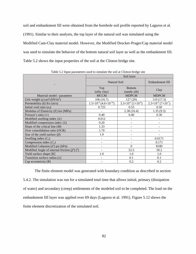
82
soil and embankment fill were obtained from the borehole soil profile reported by Laguros et al.
(1991). Similar to their analysis, the top layer of the natural soil was simulated using the
Modified Cam-Clay material model. However, the Modified Drucker-Prager/Cap material model
was used to simulate the behavior of the bottom natural soil layer as well as the embankment fill.
Table 5.2 shows the input properties of the soil at the Clinton bridge site.
Table 5.2 Input parameters used to simulate the soil at Clinton bridge site
-
Soil layer
Natural Soil Embankment fill
Top
(silty clay)
Bottom
(sandy silt) Clay
Material model / parameter MCCM MDPCM MDPCM
Unit weight (ɣ) pcf (kN/m3) 106 (16.7) 127 (20) 110 (17.3)
Permeability (k) ft/s (m/s) 1.5×10⁻⁹ (4.6×10⁻¹⁰) 3.3×10⁻⁶ (1×10⁻⁶) 2.3×10⁻⁶ (7×10⁻⁷)
Initial void ratio (e0) 0.725 0.53 0.50
Modulus of Elasticity (E) ksi (MPa) - 2.38 (16.4) 1.35 (9.3)
Poisson’s ratio (ѵ) 0.40 0.40 0.30
Modified swelling index (𝜅) 0.012 - -
Modified compression index (𝜆) 0.20 - -
Slope of the critical line (M) 1.33 - -
Over consolidation ratio (OCR) 1.70 - -
Size of the yield surface (β) 1.0 - -
Swelling index (Cs) - - 0.0171
Compression index (Cc) - - 0.171
Modified Cohesion [d'] psi (kPa) - 0 8180
Modified Angle of internal friction [β'] (0) - 52.5 50.2
Yield surface shape [K] 1.0 1.0 1.0
Transition surface radius [α] - 0.1 0.1
Cap eccentricity [R] - 0.2 0.2
The finite element model was generated with boundary condition as described in section
5.4.2. The simulation was run for a simulated total time that allows initial, primary (dissipation
of water) and secondary (creep) settlements of the modeled soil to be completed. The load on the
embankment fill layer was applied over 69 days (Laguros et al. 1991). Figure 5.12 shows the
finite element discretization of the simulated soil.

83
Figure 5.12 Finite element discretization of the simulated soil at Clinton bridge site
The results from the finite element analysis are presented in Figures 5.13 through 5.17.
Figure 5.13 shows the vertical deformation contour of the simulated soils at the end of the
analysis. Figure 5.14 shows the distribution of pore pressure at the end of the analysis.
Figure 5.13 Vertical deformation contour at the end of the analysis (ft)
Figure 5.14 Excess pore pressure contour at the end of the analysis (psf)
Figure 5.15 shows the surface settlement profile of the natural soil. The figure indicates
that the ultimate surface settlement under the center of the embankment was 5.7 in (142 mm),
which compared with the simulation result of Laguros et al. (1991) with a relatively good
agreement. The slight difference in the deflection shape could be attributed to the loading
procedure and element size used in the presented simulation. Figure 5.16 shows the surface
settlement profile at the surface of the embankment layer. A surface settlement of 7.3 in (185
mm) was encountered at the center of the embankment fill. This was in good agreement with the

84
reported settlement of 8 in (203 mm). The difference between the reported and simulated
settlement can be attributed to the maintenance performed on this bridge-site in which resurfaced
several times, which was not considered in the analysis.
Figure 5.15 Simulated surface settlement profile of the natural soil
0 15 30 45 60 75 90 105
-25
0
25
50
75
100
125
150
-1
0
1
2
3
4
5
6
0 50 100 150 200 250 300 350
Distance from plane of symmetry (m)
Ver
tica
l d
isp
lace
men
t (m
m)
Ver
tica
l d
isp
lace
men
t (i
n)
Distance from plane of symmetry (ft)
Transverse settlement profile
FEM simulation
Laguros et al. (1991) simulation

85
Figure 5.16 Simulated surface settlement profile of the embankment fill
Figure 5.17 shows excess pore pressure history at the center of the silty clay layer. The
figure shows how excess pore pressure increases as the embankment is constructed. The pore
pressure peaked at time right after the end of the embankment’s construction. A maximum pore
pressure of 1020 psf (49 kPa) was encountered. This was higher than what obtained by Laguros
et al. (1991) simulation of 500 psf (24 kPa). The difference could be attributed to the use of the
modeled embankment fill in which allowed the buildup of the pore pressure. The figure also
indicates that it took the natural soil layer (silty clay) about 7 years to reach a degree of
consolidation of 95%.
0 1.5 3 4.5 6 7.5
125
150
175
200
225
250
0
1
2
3
4
5
6
7
8
9
10
0 5 10 15 20 25
Distance from plane of symmetry (m)
Ver
tica
l d
isp
lace
men
t (m
m)
Ver
tica
l d
isp
lace
men
t (i
n)
Distance from plane of symmetry (ft)
Transverse settlement profile
Reported by Laguros et al. (1991)
Simulated settlement profile
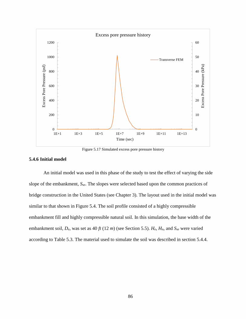
86
Figure 5.17 Simulated excess pore pressure history
5.4.6 Initial model
An initial model was used in this phase of the study to test the effect of varying the side
slope of the embankment, Sse. The slopes were selected based upon the common practices of
bridge construction in the United States (see Chapter 3). The layout used in the initial model was
similar to that shown in Figure 5.4. The soil profile consisted of a highly compressible
embankment fill and highly compressible natural soil. In this simulation, the base width of the
embankment soil, De, was set as 40 ft (12 m) (see Section 5.5). He, Hn, and Sse were varied
according to Table 5.3. The material used to simulate the soil was described in section 5.4.4.
0
10
20
30
40
50
60
0
200
400
600
800
1000
1200
1E+1 1E+3 1E+5 1E+7 1E+9 1E+11 1E+13
Exce
ss P
ore
Pre
ssure
(kP
a)
Exce
ss P
ore
Pre
ssure
(p
sf)
Time (sec)
Excess pore pressure history
Transverse FEM

87
Table 5.3 Parameters range used in the initial model simulation
Analysis No.
Side slope of the embankment fill
(Sse)
(vertical to horizontal)
Height of embankment fill
(He)
ft (m)
Height of natural soil
(Hn)
ft (m)
1
1 to 2
30 (9.1)
30 (9.1)
2 20 (6.1)
3 10 (3.0)
4
1 to 1.5
30 (9.1)
5 20 (6.1)
6 10 (3.0)
The surface settlement at the center of the embankment fill was retrieved at the end of
each analysis. Figures 5.18 through 5.23 show the deformed contour of the simulated soils.
Figure 5.24 shows the simulated surface settlement at the center of the embankment fill.
Figure 5.18 Vertical deformation contour of analysis No.1 (ft)
Figure 5.19 Vertical deformation contour of analysis No.2 (ft)

88
Figure 5.20 Vertical deformation contour of analysis No.3 (ft)
Figure 5.21 Vertical deformation contour of analysis No.4 (ft)
Figure 5.22 Vertical deformation contour of analysis No.5 (ft)
Figure 5.23 Vertical deformation contour of analysis No.6 (ft)
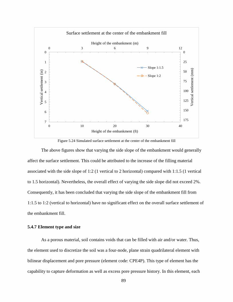
89
Figure 5.24 Simulated surface settlement at the center of the embankment fill
The above figures show that varying the side slope of the embankment would generally
affect the surface settlement. This could be attributed to the increase of the filling material
associated with the side slope of 1:2 (1 vertical to 2 horizontal) compared with 1:1.5 (1 vertical
to 1.5 horizontal). Nevertheless, the overall effect of varying the side slope did not exceed 2%.
Consequently, it has been concluded that varying the side slope of the embankment fill from
1:1.5 to 1:2 (vertical to horizontal) have no significant effect on the overall surface settlement of
the embankment fill.
5.4.7 Element type and size
As a porous material, soil contains voids that can be filled with air and/or water. Thus,
the element used to discretize the soil was a four-node, plane strain quadrilateral element with
bilinear displacement and pore pressure (element code: CPE4P). This type of element has the
capability to capture deformation as well as excess pore pressure history. In this element, each
0 3 6 9 12
0
25
50
75
100
125
150
175
0
1
2
3
4
5
6
7
0 10 20 30 40
Height of the embankment (m)
Ver
tica
l se
ttle
men
t (m
m)
Ver
tica
l se
ttle
men
t (i
n)
Height of the embankment (ft)
Surface settlement at the center of the embankment fill
Slope 1:1.5
Slope 1:2

90
node consists of two displacement degrees of freedom (Ux and Uy) and one pore pressure degree
of freedom (Por) (ABAQUS 2015). Figure 5.25 shows the element type and degrees of freedom
used in the simulation.
Figure 5.25 Element used to simulate the soil
The initial model (Section 5.4.6) was used to determine the proper element sizes that
would maintain the accuracy of results while reducing the computational time. This was done by
monitoring the surface settlement at the center of the embankment fill as a function of different
element sizes.
The soil profile used in this simulation had a layout similar to what shown in Figure 5.4.
It consisted of highly compressible embankment fill with height He = 30 ft (9.1 m), highly
compressible natural soil with height Hn = 30 ft (9.1 m), base width of the embankment fill De =
40 ft (12m), base width of the sloped part of the embankment fill Dse = 60 ft (18 m), side slope of
the embankment fill Sse = 1:2 (1 vertical to 2 horizontal), and base width of the natural soil Dn =
200 ft (61 m).
The element size was reduced in each subsequent simulation and surface settlement at the
center of the embankment fill was obtained accordingly. Table 5.4 shows the size and number of
the elements used in the analysis. Figure 5.27 shows the result of this analysis.

91
Table 5.4 Size and number of the elements used in the analysis
Element size
(length × width)
ft × ft (m × m)
Total number of elements
5.0 × 5.0 (1.5 × 1.5) 351
2.5 × 2.5 (0.8 × 0.8) 2,214
1.0 × 1.0 (0.3 × 0.3) 8,856
0.5 × 0.5 (0.2 × 0.2) 35,471
0.25 × 0.25 (0.1 × 0.1) 141,884
Figure 5.26 Simulated surface settlement at the center of the embankment fill with respect to element size
The above figure shows that the surface settlement at the center of the embankment fill
becomes nearly steady (maximum 0.04% error) when the element size is at or less than 1.0 ft ×
1.0 ft (0.30 m × 0.30 m), and therefore, this element size was used in this study.
5.5 Parametric study on transverse two-dimensional FEM
A parametric study was conducted using finite element analysis to quantify the effects of
various parameters on the surface settlement profile of the embankment fill. The parameters
considered were the height of embankment fill, He, embankment soil type, side slope of the
0 0.3 0.6 0.9 1.2 1.5 1.8
154
154.25
154.5
154.75
155
155.25
155.56.06
6.07
6.08
6.09
6.10
6.11
6.12
0 1 2 3 4 5 6
Element size (m × m)
Ver
tica
l se
ttle
men
t (m
m)
Ver
tica
l se
ttle
men
t (i
n)
Element size (ft × ft)
Surface settlement at the center of the embankment fill
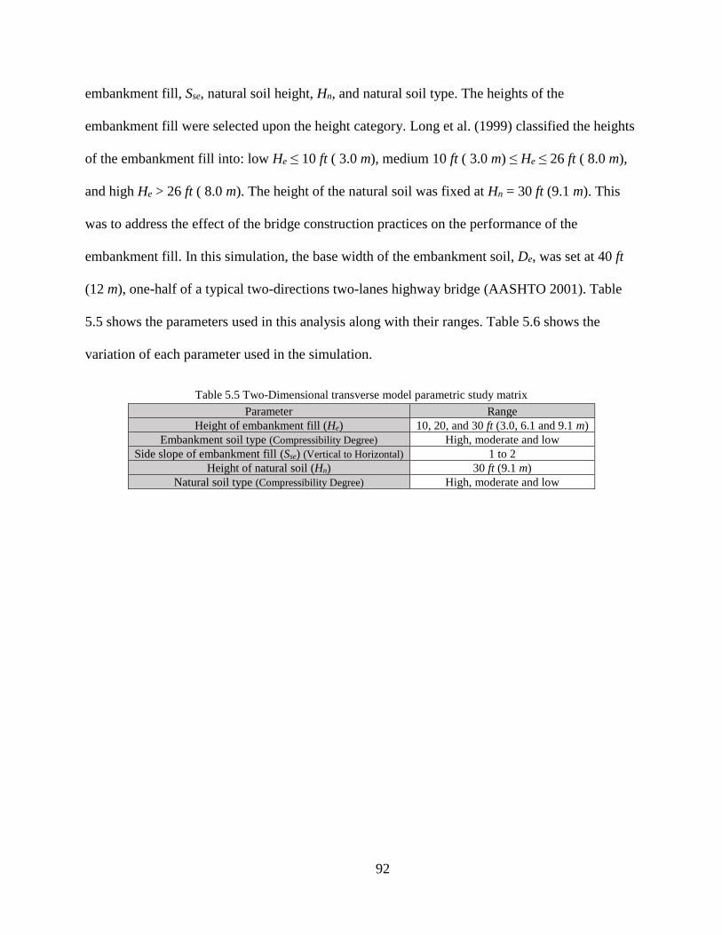
92
embankment fill, Sse, natural soil height, Hn, and natural soil type. The heights of the
embankment fill were selected upon the height category. Long et al. (1999) classified the heights
of the embankment fill into: low He ≤ 10 ft ( 3.0 m), medium 10 ft ( 3.0 m) ≤ He ≤ 26 ft ( 8.0 m),
and high He > 26 ft ( 8.0 m). The height of the natural soil was fixed at Hn = 30 ft (9.1 m). This
was to address the effect of the bridge construction practices on the performance of the
embankment fill. In this simulation, the base width of the embankment soil, De, was set at 40 ft
(12 m), one-half of a typical two-directions two-lanes highway bridge (AASHTO 2001). Table
5.5 shows the parameters used in this analysis along with their ranges. Table 5.6 shows the
variation of each parameter used in the simulation.
Table 5.5 Two-Dimensional transverse model parametric study matrix
Parameter Range
Height of embankment fill (He) 10, 20, and 30 ft (3.0, 6.1 and 9.1 m)
Embankment soil type (Compressibility Degree) High, moderate and low
Side slope of embankment fill (Sse) (Vertical to Horizontal) 1 to 2
Height of natural soil (Hn) 30 ft (9.1 m)
Natural soil type (Compressibility Degree) High, moderate and low

93
Table 5.6 Range of parameters used in the simulation
Analysis
No.
Side slope of
embankment fill (Sse) (Vertical to Horizontal)
Height of
embankment fill
(He) ft (m)
Embankment soil
type (compressibility
degree)
Natural soil type (compressibility
degree)
Height of
natural soil
(Hn) ft (m)
1
1 to 2
10 (3)
High
High
30 (9.1)
2 20 (6.1)
3 30 (9.1)
4 10 (3)
Moderate 5 20 (6.1)
6 30 (9.1)
7 10 (3)
Low 8 20 (6.1)
9 30 (9.1)
10 10 (3)
High
Moderate
11 20 (6.1)
12 30 (9.1)
13 10 (3)
Moderate 14 20 (6.1)
15 30 (9.1)
16 10 (3)
Low 17 20 (6.1)
18 30 (9.1)
19 10 (3)
High
Low
20 20 (6.1)
21 30 (9.1)
22 10 (3)
Moderate 23 20 (6.1)
24 30 (9.1)
25 10 (3)
Low 26 20 (6.1)
27 30 (9.1)
The finite element model was generated as described in section 5.4. The models were run
for a simulated total time that allowed the completion of initial, primary (dissipation of water),
and secondary (creep) settlements of the modeled soil. The load on the embankment fill was
applied according to equation 5-1. Additional surcharge pressure was applied on the top surface
of the embankment. The pressure was equivalent to the load induced by the approach
slab/pavement of 150 pcf (24 kN/m3). A typical finite element discretization of the two-
dimensional transverse model is shown in Figure 5.27. Figure 5.28 shows the simulated surface
settlement at the center of the embankment.

94
Figure 5.27 Finite element discretization of the two-dimensional transverse model
Figure 5.28 Surface settlement at the center of the embankment fill of the Two-Dimensional transverse model
The above figure shows that the height of the embankment fill has a significant effect on
the overall surface settlement. In order to put the results into perspective, one end of a 20 ft (6.1
m) approach slab was assumed to be rested on the surface of the embankment fill, and the
resulting differential settlement was evaluated accordingly (see Section 2.1). As a result,
employing a low embankment fill height of 10 ft (3.0 m) would yield a slope of (0.3/125 –
0.5/125), which in this case, would always result in a smooth slope change between the bridge
0 1.5 3 4.5 6 7.5 9 10.5
0
25
50
75
100
125
150
1750
1
2
3
4
5
6
7
0 5 10 15 20 25 30 35
Height of the embankment fill (m)
Ver
tica
l se
ttle
men
t (m
m)
Ver
tica
l se
ttle
men
t (i
n)
Height of the embankment fill (ft)
Surface settlement at the center of the embankment fill
Analysis#1-3
Analysis#4-6
Analysis#7-9
Analysis#10-12
Analysis#13-15
Analysis#16-18
Analysis#19-21
Analysis#22-24
Analysis#25-27

95
and the roadway pavement. Employing a medium embankment fill height of 20 ft (6.1 m) would
yield a slope of (0.8/125 – 1.7/125), which in this case, would fluctuate between smooth to rough
transition based upon the soil conditions. On the other hand, employing a high embankment fill
height of 30 ft (9.1 m) would yield a slope of (> 1.5/125), which in this case, would always result
in a rough transition between the bridge and the roadway pavement. Ultimately, it can be
concluded that embankment fill height of He > 20 ft (6.1 m) would be problematic in terms of the
transition performance. The slope of the approach slab must be checked against soil conditions in
such cases.
Figures 5.29 to 5.31 show the excess pore pressure history at the middle of the natural
soil layer. The figures indicate that it would take between 2 months (analysis#27) to 14 years
(analysis#1) for the natural soil layer to reach 95% consolidation. This variation would depend
mainly upon the soil conditions, i.e. height and type of the soils.
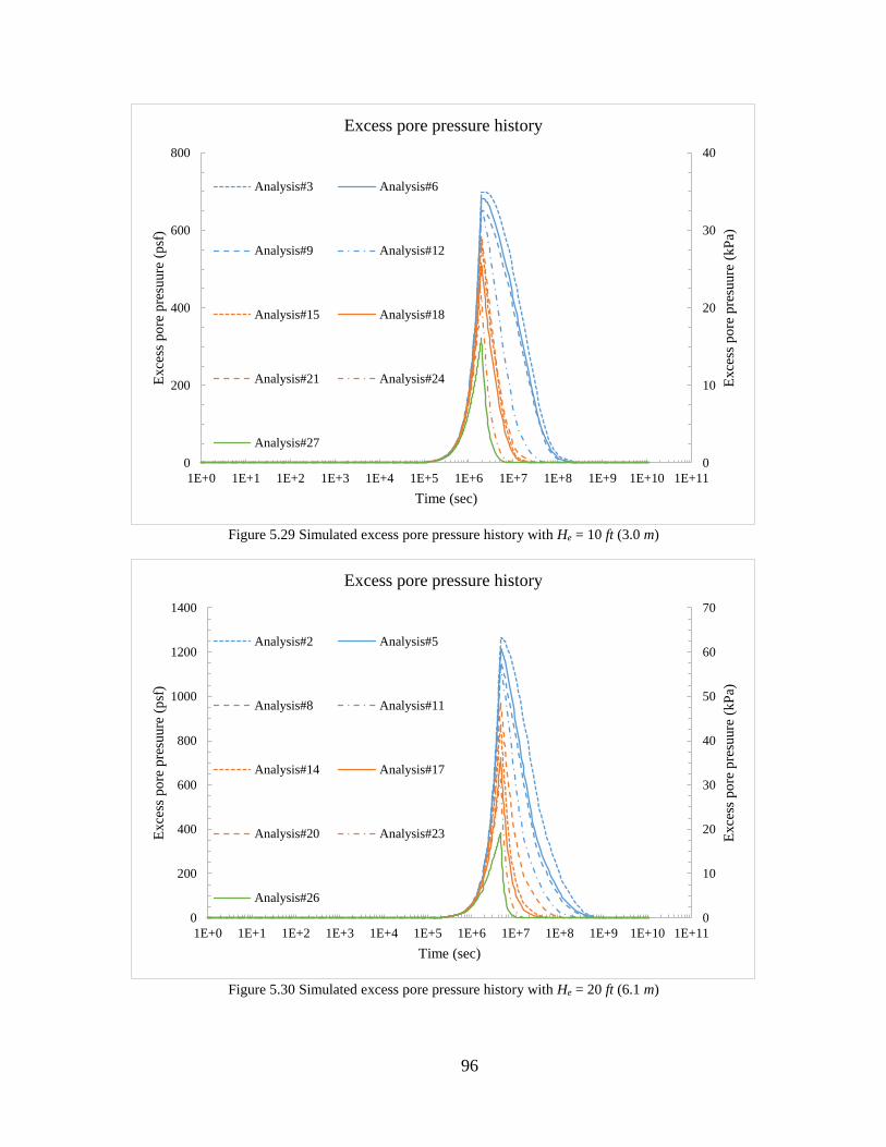
96
Figure 5.29 Simulated excess pore pressure history with He = 10 ft (3.0 m)
Figure 5.30 Simulated excess pore pressure history with He = 20 ft (6.1 m)
0
10
20
30
40
0
200
400
600
800
1E+0 1E+1 1E+2 1E+3 1E+4 1E+5 1E+6 1E+7 1E+8 1E+9 1E+10 1E+11
Exce
ss p
ore
pre
suure
(kP
a)
Exce
ss p
ore
pre
suure
(p
sf)
Time (sec)
Excess pore pressure history
Analysis#3 Analysis#6
Analysis#9 Analysis#12
Analysis#15 Analysis#18
Analysis#21 Analysis#24
Analysis#27
0
10
20
30
40
50
60
70
0
200
400
600
800
1000
1200
1400
1E+0 1E+1 1E+2 1E+3 1E+4 1E+5 1E+6 1E+7 1E+8 1E+9 1E+10 1E+11
Exce
ss p
ore
pre
suure
(kP
a)
Exce
ss p
ore
pre
suure
(p
sf)
Time (sec)
Excess pore pressure history
Analysis#2 Analysis#5
Analysis#8 Analysis#11
Analysis#14 Analysis#17
Analysis#20 Analysis#23
Analysis#26
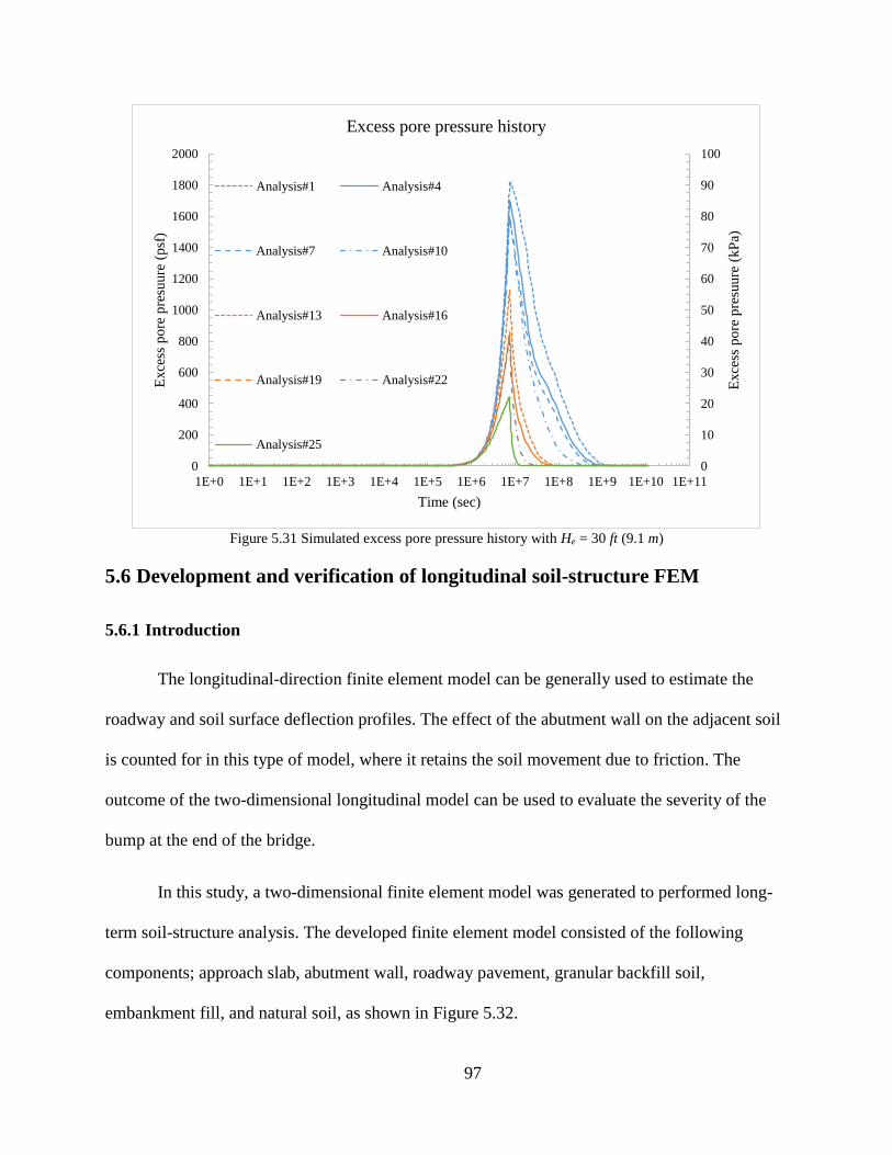
97
Figure 5.31 Simulated excess pore pressure history with He = 30 ft (9.1 m)
5.6 Development and verification of longitudinal soil-structure FEM
5.6.1 Introduction
The longitudinal-direction finite element model can be generally used to estimate the
roadway and soil surface deflection profiles. The effect of the abutment wall on the adjacent soil
is counted for in this type of model, where it retains the soil movement due to friction. The
outcome of the two-dimensional longitudinal model can be used to evaluate the severity of the
bump at the end of the bridge.
In this study, a two-dimensional finite element model was generated to performed long-
term soil-structure analysis. The developed finite element model consisted of the following
components; approach slab, abutment wall, roadway pavement, granular backfill soil,
embankment fill, and natural soil, as shown in Figure 5.32.
0
10
20
30
40
50
60
70
80
90
100
0
200
400
600
800
1000
1200
1400
1600
1800
2000
1E+0 1E+1 1E+2 1E+3 1E+4 1E+5 1E+6 1E+7 1E+8 1E+9 1E+10 1E+11
Exce
ss p
ore
pre
suure
(kP
a)
Exce
ss p
ore
pre
suure
(p
sf)
Time (sec)
Excess pore pressure history
Analysis#1 Analysis#4
Analysis#7 Analysis#10
Analysis#13 Analysis#16
Analysis#19 Analysis#22
Analysis#25

98
Figure 5.32 Two-dimensional longitudinal model layout
5.6.2 Geometry and boundary conditions
An important aspect of the soil-structure finite element model is selecting the location
and types of boundary conditions (i.e. displacement and/or pore pressure boundary conditions) in
an efficient and effective manner. Typically, the bottom of the model would represent a location
where no soil movement occurs (vertical and horizontal). This location can be determined using
the standard penetration test (typically provided in the borehole log profile) whereas a high value
indicates a hard layer, such as bedrock. At this location, both vertical and horizontal movements
are restricted (assumed to be zero). In addition, no water seepage would be expected to occur at
this location, thus, impervious boundary was assumed. The top surfaces of the soil were free to
move in all directions. Furthermore, water would be expected to flow through the top surfaces,
thus, pervious boundary was assumed.
The soil mass must be sufficiently extended in the longitudinal direction to capture the
behavior of the soil. Briaud and Lim (1997) recommend extending the soil mass to a distance of
3(He + Hn) from the back of the abutment wall to one end of the embankment model, Le, and a
distance of 3Hn to the opposite end of the model, Le. The He and Hn parameters are the heights of

99
the embankment fill and natural soil, respectively (Figure 5.33). Along these vertical boundaries,
the soil was assumed to move in the vertical direction only.
The nodes at the bottom of the abutment were fixed against horizontal and vertical
movements, representing foundation support. The approach slab was connected to the abutment
with a pin connection at the middle of the approach slab. This connection restricts the relative
horizontal and vertical movements between the approach slab and the abutment while allowing
free rotation. Figures 5.33 and 5.34 show the geometric and boundary condition parameters used
in the finite element model for bridges with wall and stub abutments, respectively. Figure 5.35
shows the connections between the approach slab and the abutment and between the abutment
wall and its foundation.
Figure 5.33 Layout of the two-dimensional longitudinal model with wall abutment
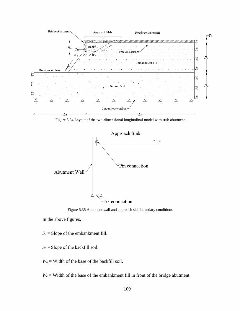
100
Figure 5.34 Layout of the two-dimensional longitudinal model with stub abutment
Figure 5.35 Abutment wall and approach slab boundary conditions
In the above figures,
Se = Slope of the embankment fill.
Sb = Slope of the backfill soil.
Wb = Width of the base of the backfill soil.
We = Width of the base of the embankment fill in front of the bridge abutment.

101
Ha = Height of the abutment wall.
Ta = Thickness of the abutment wall.
Ls = Length of the approach slab.
Ts = Thickness of the approach slab.
In this study, He, Hn, Ha, and Sb were varied according to the study matrix found in Table
5.9. Le and Ln were fixed at 180 ft (55 m), and 90 ft (27 m), respectively. They were determined
as a function of the embankment fill and natural soil heights. Ls, Ts, Ta, Wb, We, were fixed at 20
ft (6.1 m), 12 in (305 mm), 2 ft (0.6 m), and 3 ft (0.9 m), respectively. In addition, Se was fixed at
1:1.5 (1 vertical to 1.5 horizontal). These geometries were chosen to reflect the most common
bridge-construction practices across the United States (see Chapter 3).
5.6.3 Contact behavior at structure-soil interfaces
The developed two-dimensional finite element model involves the interaction between
the several structural components and the soil (i.e. abutment wall with soil, approach slab with
soil, and roadway pavement with soil). Interface elements were introduced across these
interfaces in order to transfer the load in the normal as well as tangential directions using the
pressure-overclosure relationship as well as coulomb friction model defined within ABAQUS
(see Section 4.2). In this analysis, the concrete surfaces (i.e. abutment wall, approach slab, and
roadway pavement) were assigned to behave as master elements while soil surfaces were
assigned to behave as slave elements.

102
5.6.4 Analysis procedures for longitudinal soil-structure model
The analysis procedures used to run the longitudinal soil-structure model included the
following steps:
1- Applying a geostatic load on the natural soil layer. In this step, the effective self-
weight of the natural soil was applied. The geostatic step assures that equilibrium
is satisfied within the natural soil layer, and that the initial stress condition in all
elements falls within the initial yield surface.
2- Constructing the embankment fill and bridge abutment over a period of time. In
this step, the effective self-weight of the embankment soil and abutment was
applied. This is done in a coupled (consolidation) step where the load of the
embankment is applied in a timely manner using equation 5-1.
3- Adding the approach slab, and roadway pavement. This is also done in a coupled
(consolidation) step where the load of the approach slab and roadway pavement
was applied in a timely manner. The construction of the approach slab and
roadway pavement was assumed to occur after the completion of the embankment
fill and assumed to be constructed over a ten-day period.
4- Consolidation step/steps. In this step/steps, the calculations of the primary
settlement (consolidation process) and secondary settlement (creep) were made.
5.6.5 Material properties
The concrete in the abutment wall, approach slab, and roadway pavement was assumed to
behave in a linearly elastic manner with a modulus of elasticity that was consistent with a design
compressive strength of 4000 psi. Table 4.2 shows the input parameters used to simulate the

103
concrete. On the other hand, the modified Drucker-Prager/Cap material model was used to
simulate the behavior of the soils. Table 4.7 shows the input parameters used to model the soil.
5.6.6 Verification analysis
In this part of the study, an attempt was made to evaluate the longitudinal surface
settlement profile at the Clinton bridge-site (see Section 5.4.5.2 for detailed description of the
Clinton bridge-site). The soil profile consisted of clay embankment layer with height He = 25 ft
(7.5 m) and two natural soil layers; top silty clay with height Hn-Top =14 ft (4.3 m) and bottom
sandy silt layer with height Hn-Bottom = 8 ft (2.4 m). No information was provided regarding the
approach slab length, backfill material, and abutment type/height. An assumed approach slab
length Ls = 20 ft (6.1 m), and thickness Ts = 13 in (330 mm) were used in this simulation. The
backfill material was assumed to be compacted to 90% of the standard proctor value with side
slope Sb = 1:1 (1 vertical to 1 horizontal). These assumptions were based upon the information
found in Oklahoma’s bridge manual (see Section 3.5). The abutment wall was assumed as wall
abutment with height Ha = He and thickness Ta = 2 ft (0.6 m). Accordingly, Ln and Le were set as
66 ft (20 m) and 141 ft (43 m), respectively. They were determined based on Briaud and Lim
(1997) recommendation (see Section 5.6.2). The layout of the FEM used in this simulation is
shown in Figure 5.36.

104
Figure 5.36 Boundary condition used for the longitudinal verification FEM
The finite element model was generated as described in sections 5.6.1 through 5.6.5.
Table 5.2 shows the input parameters used to simulate the natural and embankment layers. Table
4.7 shows the input parameters used to simulate the backfill material. The FEM was run for a
simulated total time that allows initial, primary (dissipation of water) and secondary (creep)
settlements of the modeled soil to be completed. The load on the embankment/backfill fill layers
was applied according to equation 5-1. An additional approach slab and roadway pavement self-
weight of 150 pcf (24 kN/m3) was applied on the top surface of the embankment fill. The finite
element discretization of the verification model is shown in Figure 5.37. Figures 5.38 and 5.39
show the deformed contour of the vertical deformation and excess pore pressure at the end of the
analysis, respectively.

105
Figure 5.37 Finite element discretization of the longitudinal direction at Clinton bridge site
Figure 5.38 Vertical deformation contour at the end of the analysis (ft)
Figure 5.39 Excess pore pressure contour at the end of the analysis (psf)
Figure 5.40 shows the simulated longitudinal settlement profile for the roadway surface
as well as the underneath soil. The FEM analysis shows a settlement of 8.5 in (216 mm) at a
distance of 71 ft (21.6 m) from the bridge abutment. Within the approach slab, a differential
settlement of 7.4 in (188 mm) was observed. This was compared with the history settlement
reported by Laguros et al. (1991) of 8 in (203 mm) with a relatively good agreement. The
difference between the reported and FEM analysis could be attributed to the type of model used
in this simulation (see Section 5.9.1.1).

106
Figure 5.40 Simulated longitudinal settlement profiles at Clinton bridge-site
Figure 5.41 shows the simulated history of the excess pore pressure of the silty clay layer
(first layer of the natural soil) at a distance away from the bridge. The pore pressure history was
compared with the history obtained from the transverse settlement (see Section5.4.5.2) with a
good agreement.
0 6 12 18 24 30 36 42 48
0
25
50
75
100
125
150
175
200
225
250
0
1
2
3
4
5
6
7
8
9
10
0 20 40 60 80 100 120 140 160
Distance from the bridge (m)
Ver
tica
l se
ttle
men
t (m
m)
Ver
tica
l se
ttle
men
t (i
n)
Distance from the bridge (ft)
Longitudinal settlement profile behind bridge abutment
FEM Roadway settlement profile
FEM Soil settlement profile
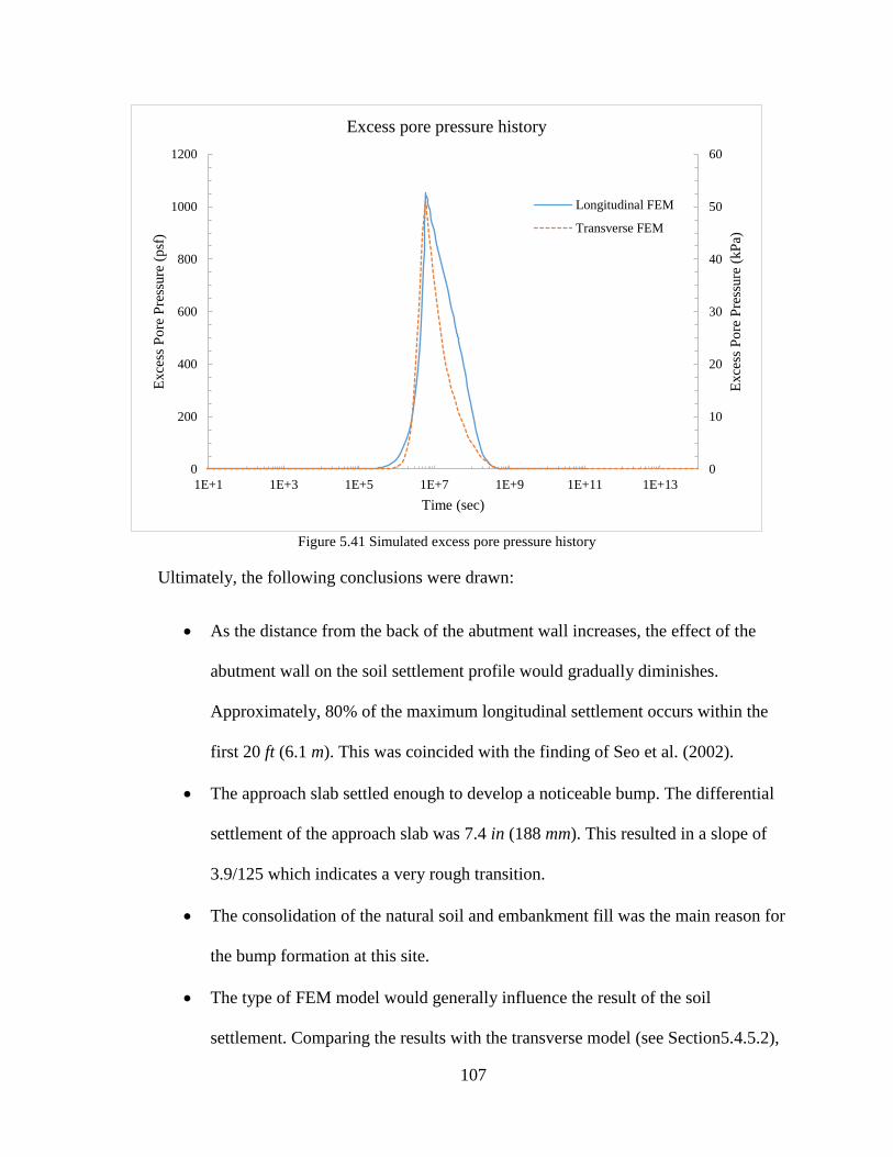
107
Figure 5.41 Simulated excess pore pressure history
Ultimately, the following conclusions were drawn:
• As the distance from the back of the abutment wall increases, the effect of the
abutment wall on the soil settlement profile would gradually diminishes.
Approximately, 80% of the maximum longitudinal settlement occurs within the
first 20 ft (6.1 m). This was coincided with the finding of Seo et al. (2002).
• The approach slab settled enough to develop a noticeable bump. The differential
settlement of the approach slab was 7.4 in (188 mm). This resulted in a slope of
3.9/125 which indicates a very rough transition.
• The consolidation of the natural soil and embankment fill was the main reason for
the bump formation at this site.
• The type of FEM model would generally influence the result of the soil
settlement. Comparing the results with the transverse model (see Section5.4.5.2),
0
10
20
30
40
50
60
0
200
400
600
800
1000
1200
1E+1 1E+3 1E+5 1E+7 1E+9 1E+11 1E+13
Exce
ss P
ore
Pre
ssure
(kP
a)
Exce
ss P
ore
Pre
ssure
(p
sf)
Time (sec)
Excess pore pressure history
Longitudinal FEM
Transverse FEM

108
the far away soil settlement of 8.6 in (218 mm) resulted from the longitudinal
model was greater than 7.3 in (185 mm) resulted from the transverse model. This
could be attributed to the effect side slope of the embankment Sse, which was not
considered. A later study confirmed this finding (see Section 5.9.1.1)
5.6.7 Initial model
An initial model was used in this phase of the study to test the effect of the erosion of the
backfill material. A hypothesis trench size of 3:6 (3 vertical to 6 horizontal) was simulated to
examine its effect on the approach slab performance (resulting slope). The erosion was assumed
to fully developed eight months after the end of the bridge construction, i.e. eight months after
the bridge is open to the public. Figure 5.42 shows the layout of the trench simulation.
Figure 5.42 Layout of the initial model (wall abutment)
The soil profile used in this simulation consisted of a granular backfill, highly
compressible embankment fill and high compressible natural soil. In this analysis, Sb = 1:2 (1
vertical to 2 horizontal), He = 30 ft (9.1 m) and Hn = 30 ft (9.1 m). Three abutment wall heights,
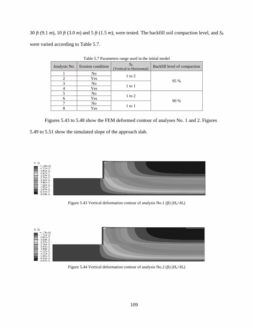
109
30 ft (9.1 m), 10 ft (3.0 m) and 5 ft (1.5 m), were tested. The backfill soil compaction level, and Sb
were varied according to Table 5.7.
Table 5.7 Parameters range used in the initial model
Analysis No. Erosion condition Sb
(Vertical to Horizontal) Backfill level of compaction
1 No 1 to 2
95 % 2 Yes
3 No 1 to 1
4 Yes
5 No 1 to 2
90 % 6 Yes
7 No 1 to 1
8 Yes
Figures 5.43 to 5.48 show the FEM deformed contour of analyses No. 1 and 2. Figures
5.49 to 5.51 show the simulated slope of the approach slab.
Figure 5.43 Vertical deformation contour of analysis No.1 (ft) (Ha=He)
Figure 5.44 Vertical deformation contour of analysis No.2 (ft) (Ha=He)

110
Figure 5.45 Vertical deformation contour of analysis No.1 (ft) (Ha=10 ft)
Figure 5.46 Vertical deformation contour of analysis No.2 (ft) (Ha=10 ft)
Figure 5.47 Vertical deformation contour of analysis No.1 (ft) (Ha=5 ft)
Figure 5.48 Vertical deformation contour of analysis No.2 (ft) (Ha=5 ft)
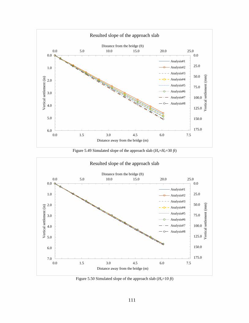
111
Figure 5.49 Simulated slope of the approach slab (Ha=He=30 ft)
Figure 5.50 Simulated slope of the approach slab (Ha=10 ft)
0.0 1.5 3.0 4.5 6.0 7.5
0.0
25.0
50.0
75.0
100.0
125.0
150.0
175.0
0.0
1.0
2.0
3.0
4.0
5.0
6.0
0.0 5.0 10.0 15.0 20.0 25.0
Distance away from the bridge (m)
Ver
tica
l se
ttle
men
t (m
m)
Ver
tica
l se
ttle
men
t (i
n)
Distance from the bridge (ft)
Resulted slope of the approach slab
Analysis#1
Analysis#2
Analysis#3
Analysis#4
Analysis#5
Analysis#6
Analysis#7
Analysis#8
0.0 1.5 3.0 4.5 6.0 7.5
0.0
25.0
50.0
75.0
100.0
125.0
150.0
175.0
0.0
1.0
2.0
3.0
4.0
5.0
6.0
7.0
0.0 5.0 10.0 15.0 20.0 25.0
Distance away from the bridge (m)
Ver
tica
l se
ttle
men
t (m
m)
Ver
tica
l se
ttle
men
t (i
n)
Distance from the bridge (ft)
Resulted slope of the approach slab
Analysis#1
Analysis#2
Analysis#3
Analysis#4
Analysis#5
Analysis#6
Analysis#7
Analysis#8

112
Figure 5.51 Simulated slope of the approach slab (Ha=5 ft)
It can be concluded from the above figures that the effect of introducing trench (erosion
in the backfill) on the performance of the approach slab is not significant. In fact, the resulting
slope of the approach slab with eroded backfill was, in general, less than the intact backfill. This
can be attributed to the loss of some of the backfill weight that was removed during the
simulation. Nevertheless, the overall effect on the resulting slope of the approach slab did not
exceed 2%. Consequently, it has been concluded that the erosion has no significant effect on the
overall performance of the approach slab.
5.6.8 Element type and size
As a porous material, soil contains voids that can be filled with air and/or water. Thus,
the element used to discretize the soil was a four-node, plane strain quadrilateral element with
bilinear displacement and pore pressure (element code: CPE4P). This type of element has the
capability to capture deformation as well as excess pore pressure history. In this element, each
0.0 1.5 3.0 4.5 6.0 7.5
0.0
25.0
50.0
75.0
100.0
125.0
150.0
175.0
0.0
1.0
2.0
3.0
4.0
5.0
6.0
7.0
0.0 5.0 10.0 15.0 20.0 25.0
Distance away from the bridge (m)
Ver
tica
l se
ttle
men
t (m
m)
Ver
tica
l se
ttle
men
t (i
n)
Distance from the bridge (ft)
Resulted slope of the approach slab
Analysis#1
Analysis#2
Analysis#3
Analysis#4
Analysis#5
Analysis#6
Analysis#7
Analysis#8
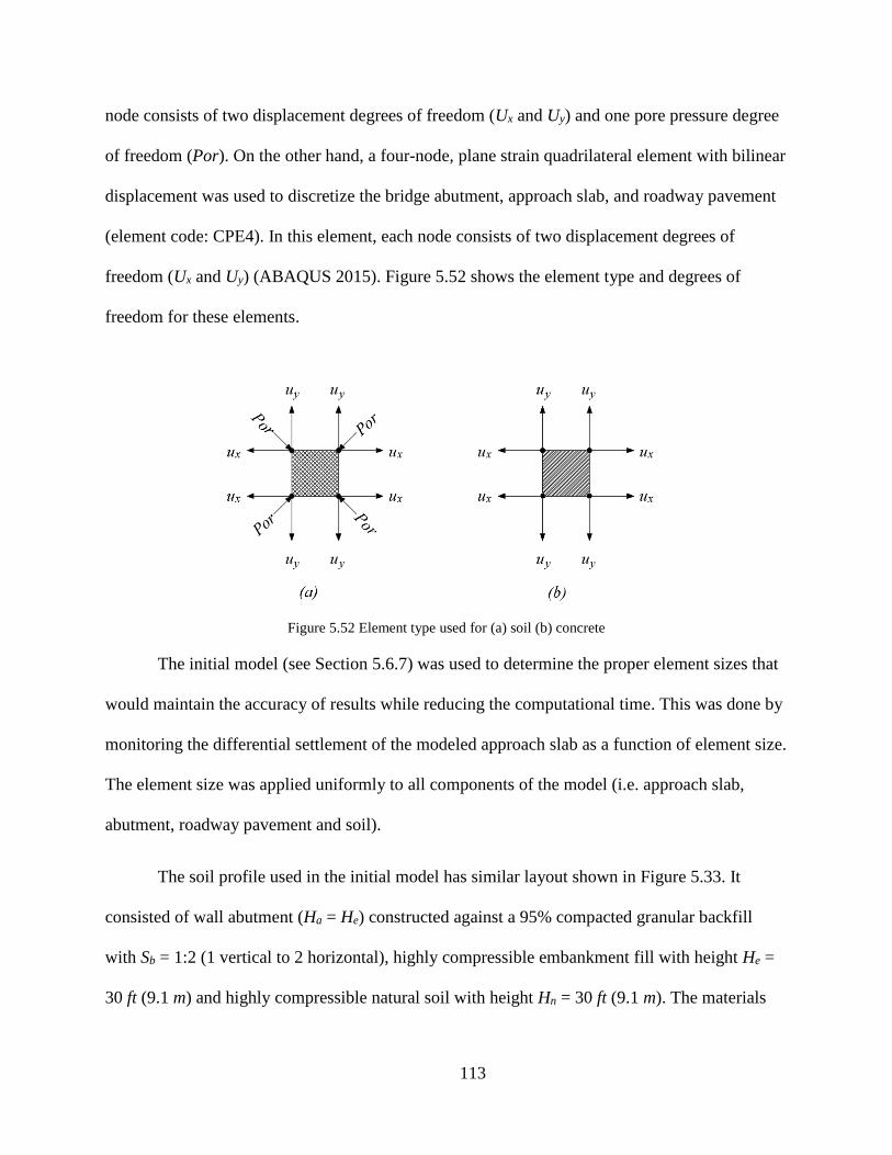
113
node consists of two displacement degrees of freedom (Ux and Uy) and one pore pressure degree
of freedom (Por). On the other hand, a four-node, plane strain quadrilateral element with bilinear
displacement was used to discretize the bridge abutment, approach slab, and roadway pavement
(element code: CPE4). In this element, each node consists of two displacement degrees of
freedom (Ux and Uy) (ABAQUS 2015). Figure 5.52 shows the element type and degrees of
freedom for these elements.
Figure 5.52 Element type used for (a) soil (b) concrete
The initial model (see Section 5.6.7) was used to determine the proper element sizes that
would maintain the accuracy of results while reducing the computational time. This was done by
monitoring the differential settlement of the modeled approach slab as a function of element size.
The element size was applied uniformly to all components of the model (i.e. approach slab,
abutment, roadway pavement and soil).
The soil profile used in the initial model has similar layout shown in Figure 5.33. It
consisted of wall abutment (Ha = He) constructed against a 95% compacted granular backfill
with Sb = 1:2 (1 vertical to 2 horizontal), highly compressible embankment fill with height He =
30 ft (9.1 m) and highly compressible natural soil with height Hn = 30 ft (9.1 m). The materials

114
used to model the concrete in the abutment wall, approach slab, and roadway pavement as well
as soil are described in section 5.6.5.
The element size was reduced in each subsequent run and settlement at the end of the
approach slab was obtained accordingly. Table 5.8 shows the size and number of the elements
used in the analysis. Figure 5.53 shows the result of this analysis.
Table 5.8 Size and number of the elements used in the analysis
Element size
(length × width)
ft × ft (m × m)
Total number of elements
5.0 × 5.0 (1.5 × 1.5) 683
2.5 × 2.5 (0.8 × 0.8) 2,467
1.0 × 1.0 (0.3 × 0.3) 15,216
0.5 × 0.5 (0.2 × 0.2) 60,143
0.25 × 0.25 (0.1 × 0.1) 241,094

115
Figure 5.53 Simulated differential settlement of approach slab with respect to element size
Figure 5.53 shows that the differential settlement of the approach slab becomes nearly
steady (maximum 0.2% error) when the element size is at or less than 1.0 ft × 1.0 ft (0.30 m ×
0.30 m), and therefore, this element size was used in this study.
5.7 Parametric study on longitudinal two-dimensional FEM
A parametric study was conducted using finite element analysis to quantify the effects of
various parameters on the soil’s longitudinal settlement profile behind the bridge abutment. The
parameters considered were the length of the approach slab, Ls, height of embankment fill, He,
embankment soil type, height of natural soil, Hn, natural soil type, backfill soil type, slope of
backfill area, Sb, and abutment type/height, Ha. Table 5.9 shows these parameters along with
their ranges.
0 0.3 0.6 0.9 1.2 1.5 1.8
118
118.5
119
119.5
120
120.5
4.65
4.68
4.70
4.73
4.75
0 1 2 3 4 5 6
Element size (m × m)
Ver
tica
l S
ettl
emen
t (m
m)
Ver
tica
l S
ettl
emen
t (i
n)
Element size (ft × ft)
Diffrential settlement of approach slab

116
To efficiently minimize the number of analyses performed in this parametric study, the
following assumptions were made. First, each soil profile was idealized into three distinct
homogenous soil layers; backfill soil, embankment fill, and natural soil. Second, only soil
profiles that were expected to cause settlements resulting in an approach slab slope of 1/125 (or
greater) were considered. This was done to exclude situations where soil settlement would not
pose a ride quality issue. Third, it was assumed that the embankment fill would never be any
worse (more prone to settlement) than the natural soil. In other words, the embankment fill
would not be more compressible than the natural soil. This is particularly the case in bridge
constructions, since the embankment fill can be either a selected (better) fill brought to the site,
or a readily available local fill from the nearby natural soil (Briaud, James and Hoffman 1997,
McLaren 1970, Dupont and Allen 2002). Table 5.10 shows the soil profiles considered in this
study.
Table 5.9 Two-Dimensional longitudinal model parametric study matrix
Parameter Value
Length of approach slab segment Ls 20 ft (6.1 m)
Height of embankment fill He 20 and 30 ft (6.1 and 9.1 m)
Embankment soil type (Compressibility Degree) High, moderate and low
Height of natural soil Hn 30 ft (9.1 m)
Natural soil type (Compressibility Degree) High, moderate and low
Backfill soil compaction level 90% and 95%
Backfill slope Sb (vertical to horizonal)
1 to 1 and 1 to 2
Abutment type/height Ha
Wall abutment/Ha = He
Stub abutment/Ha = 10 ft (3.0 m)
Stub abutment/Ha = 5 ft (1.5 m)

117
Table 5.10 Soil profiles considered in the longitudinal model parametric study
Soil profile No. Hn
ft (m)
He
ft (m)
Natural soil type
(compressibility degree)
Embankment soil type
(compressibility degree)
1
30 (9.1)
30 (9.1)
High
High
2 Moderate
3 Low
4 Moderate
Moderate
5 Low
6 Low Low
7
20 (6.1) High
High
8 Moderate
9 Low
Accordingly, each soil profile was examined using various choices of parameters to
quantify their effect on the ultimate longitudinal soil settlement profile behind the bridge
abutment. Table 5.11 shows the variations of all parameter associated with each examined soil
profile.
Table 5.11 Range of parameters used in accordance with each soil profile (refer to Table 5.10)
Analysis No. Abutment type/height
ft (m)
Backfill
level of compaction Backfill slope Sb
(vertical to horizontal)
1
Wall abutment/Ha = He
95% 1 to 2
2 1 to 1
3 90%
1 to 2
4 1 to 1
5
Stub abutment/Ha = 10 (3.0)
95% 1 to 2
6 1 to 1
7 90%
1 to 2
8 1 to 1
9
(1.5) 5= aH/Stub abutment
95% 1 to 2
10 1 to 1
11 90%
1 to 2
12 1 to 1
The finite element model was generated using material properties shown in Tables 4.2
and 4.6. The boundary conditions, analysis steps, elements types, and contact behavior were used
as described in section 5.6. The models were run for a simulated total time that allowed the
completion of initial, primary (dissipation of water), and secondary (creep) settlements of the
modeled soil. The load on the embankment fill layer was applied according to equation 5-1. An
additional approach slab and roadway pavement surcharge of 150 pcf (24 kN/m3) was applied on

118
the top surface of the embankment fill. A typical finite element discretization of the two-
dimensional longitudinal model is shown in Figure 5.54.
Figure 5.54 Finite element discretization of the two-dimensional longitudinal model
5.7.1 Differential settlement of approach slab
The differential settlement of the approach slab was the interest of this phase of the study.
The objective was to quantify the resulted approach slab slope against different abutment wall-
soil conditions (see Tables 5.10 and 5.11). The result of the finite element analysis is shown in
Figures 5.55 to 5.63.

119
Figure 5.55 Simulated slope of the approach slab for soil profile No.1
Figure 5.56 Simulated slope of the approach slab for soil profile No.2
0 1.5 3 4.5 6 7.5
0
25
50
75
100
125
150
175
0
1
2
3
4
5
6
7
0 5 10 15 20 25
Distance from the bridge (m)
Ver
tica
l se
ttle
men
t (m
m)
Ver
tica
l se
ttle
men
t (i
n)
Distance from the bridge (ft)
Resulted slope of the approach slab
Analysis#1 Analysis#2
Analysis#3 Analysis#4
Analysis#5 Analysis#6
Analysis#7 Analysis#8
Analysis#9 Analysis#10
Analysis#11 Analysis#12
0 1.5 3 4.5 6 7.5
0
25
50
75
100
125
0
1
2
3
4
5
0 5 10 15 20 25
Distance from the bridge (m)
Ver
tica
l se
ttle
men
t (m
m)
Ver
tica
l se
ttle
men
t (i
n)
Distance from the bridge (ft)
Resulted slope of the approach slab
Analysis#1 Analysis#2
Analysis#3 Analysis#4
Analysis#5 Analysis#6
Analysis#7 Analysis#8
Analysis#9 Analysis#10
Analysis#11 Analysis#12

120
Figure 5.57 Simulated slope of the approach slab for soil profile No.3
Figure 5.58 Simulated slope of the approach slab for soil profile No.4
0 1.5 3 4.5 6 7.5
0
25
50
75
100
125
0
1
2
3
4
5
0 5 10 15 20 25
Distance from the bridge (m)
Ver
tica
l se
ttle
men
t (m
m)
Ver
tica
l se
ttle
men
t (i
n)
Distance from the bridge (ft)
Resulted slope of the approach slab
Analysis#1 Analysis#2
Analysis#3 Analysis#4
Analysis#5 Analysis#6
Analysis#7 Analysis#8
Analysis#9 Analysis#10
Analysis#11 Analysis#12
0 1.5 3 4.5 6 7.5
0
25
50
75
100
0
1
2
3
4
0 5 10 15 20 25
Distance from the bridge (m)
Ver
tica
l se
ttle
men
t (m
m)
Ver
tica
l se
ttle
men
t (i
n)
Distance from the bridge (ft)
Resulted slope of the approach slab
Analysis#1 Analysis#2
Analysis#3 Analysis#4
Analysis#5 Analysis#6
Analysis#7 Analysis#8
Analysis#9 Analysis#10
Analysis#11 Analysis#12

121
Figure 5.59 Simulated slope of the approach slab for soil profile No.5
Figure 5.60 Simulated slope of the approach slab for soil profile No.6
0 1.5 3 4.5 6 7.5
0
25
50
75
100
0
1
2
3
4
0 5 10 15 20 25
Distance from the bridge (m)
Ver
tica
l se
ttle
men
t (m
m)
Ver
tica
l se
ttle
men
t (i
n)
Distance from the bridge (ft)
Resulted slope of the approach slab
Analysis#1 Analysis#2
Analysis#3 Analysis#4
Analysis#5 Analysis#6
Analysis#7 Analysis#8
Analysis#9 Analysis#10
Analysis#11 Analysis#12
0 1.5 3 4.5 6 7.5
0
25
50
75
0
1
2
3
0 5 10 15 20 25
Distance from the bridge (m)
Ver
tica
l se
ttle
men
t (m
m)
Ver
tica
l se
ttle
men
t (i
n)
Distance from the bridge (ft)
Resulted slope of the approach slab
Analysis#1 Analysis#2
Analysis#3 Analysis#4
Analysis#5 Analysis#6
Analysis#7 Analysis#8
Analysis#9 Analysis#10
Analysis#11 Analysis#12

122
Figure 5.61 Simulated slope of the approach slab for soil profile No.7
Figure 5.62 Simulated slope of the approach slab for soil profile No.8
0 1.5 3 4.5 6 7.5
0
25
50
75
100
0
1
2
3
4
0 5 10 15 20 25
Distance from the bridge (m)
Ver
tica
l se
ttle
men
t (m
m)
Ver
tica
l se
ttle
men
t (i
n)
Distance from the bridge (ft)
Resulted slope of the approach slab
Analysis#1 Analysis#2
Analysis#3 Analysis#4
Analysis#5 Analysis#6
Analysis#7 Analysis#8
Analysis#9 Analysis#10
Analysis#11 Analysis#12
0 1.5 3 4.5 6 7.5
0
25
50
75
0
1
2
3
0 5 10 15 20 25
Distance from the bridge (m)
Ver
tica
l se
ttle
men
t (m
m)
Ver
tica
l se
ttle
men
t (i
n)
Distance from the bridge (ft)
Resulted slope of the approach slab
Analysis#1 Analysis#2
Analysis#3 Analysis#4
Analysis#5 Analysis#6
Analysis#7 Analysis#8
Analysis#9 Analysis#10
Analysis#11 Analysis#12
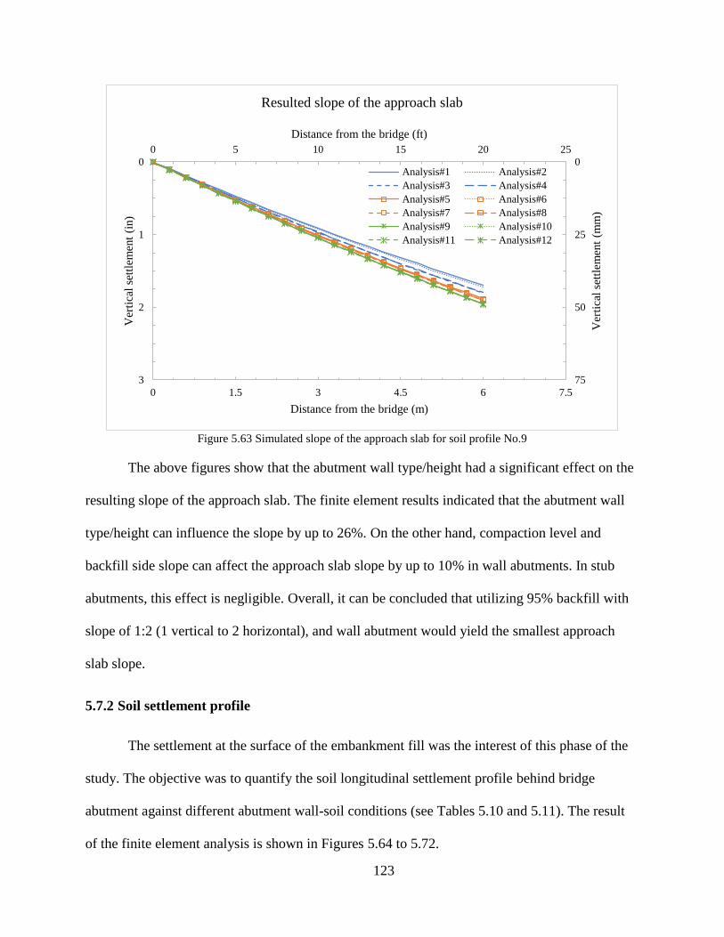
123
Figure 5.63 Simulated slope of the approach slab for soil profile No.9
The above figures show that the abutment wall type/height had a significant effect on the
resulting slope of the approach slab. The finite element results indicated that the abutment wall
type/height can influence the slope by up to 26%. On the other hand, compaction level and
backfill side slope can affect the approach slab slope by up to 10% in wall abutments. In stub
abutments, this effect is negligible. Overall, it can be concluded that utilizing 95% backfill with
slope of 1:2 (1 vertical to 2 horizontal), and wall abutment would yield the smallest approach
slab slope.
5.7.2 Soil settlement profile
The settlement at the surface of the embankment fill was the interest of this phase of the
study. The objective was to quantify the soil longitudinal settlement profile behind bridge
abutment against different abutment wall-soil conditions (see Tables 5.10 and 5.11). The result
of the finite element analysis is shown in Figures 5.64 to 5.72.
0 1.5 3 4.5 6 7.5
0
25
50
75
0
1
2
3
0 5 10 15 20 25
Distance from the bridge (m)
Ver
tica
l se
ttle
men
t (m
m)
Ver
tica
l se
ttle
men
t (i
n)
Distance from the bridge (ft)
Resulted slope of the approach slab
Analysis#1 Analysis#2
Analysis#3 Analysis#4
Analysis#5 Analysis#6
Analysis#7 Analysis#8
Analysis#9 Analysis#10
Analysis#11 Analysis#12

124
Figure 5.64 Simulated longitudinal soil settlement profile for soil profile No.1
Figure 5.65 Simulated longitudinal soil settlement profile for soil profile No.2
0 10 20 30 40 50 60
0
25
50
75
100
125
150
175
200
225
0
1
2
3
4
5
6
7
8
9
0 20 40 60 80 100 120 140 160 180 200
Distance from the bridge (m)
Ver
tica
l se
ttle
men
t (m
m)
Ver
tica
l se
ttle
men
t (i
n)
Distance from the bridge (ft)
Longitudinal settlement profile behind bridge abutment
Analysis#1 Analysis#2
Analysis#3 Analysis#4
Analysis#5 Analysis#6
Analysis#7 Analysis#8
Analysis#9 Analysis#10
Analysis#11 Analysis#12
0 10 20 30 40 50 60
0
25
50
75
100
125
150
175
0
1
2
3
4
5
6
7
0 20 40 60 80 100 120 140 160 180 200
Distance from the bridge (m)
Ver
tica
l se
ttle
men
t (m
m)
Ver
tica
l se
ttle
men
t (i
n)
Distance from the bridge (ft)
Longitudinal settlement profile behind bridge abutment
Analysis#1 Analysis#2
Analysis#3 Analysis#4
Analysis#5 Analysis#6
Analysis#7 Analysis#8
Analysis#9 Analysis#10
Analysis#11 Analysis#12

125
Figure 5.66 Simulated longitudinal soil settlement profile for soil profile No.3
Figure 5.67 Simulated longitudinal soil settlement profile for soil profile No.4
0 10 20 30 40 50 60
0
25
50
75
100
125
150
0
1
2
3
4
5
6
0 20 40 60 80 100 120 140 160 180 200
Distance from the bridge (m)
Ver
tica
l se
ttle
men
t (m
m)
Ver
tica
l se
ttle
men
t (i
n)
Distance from the bridge (ft)
Longitudinal settlement profile behind bridge abutment
Analysis#1 Analysis#2
Analysis#3 Analysis#4
Analysis#5 Analysis#6
Analysis#7 Analysis#8
Analysis#9 Analysis#10
Analysis#11 Analysis#12
0 10 20 30 40 50 60
0
25
50
75
100
0
1
2
3
4
0 20 40 60 80 100 120 140 160 180 200
Distance away from the bridge (m)
Ver
tica
l se
ttle
men
t (m
m)
Ver
tica
l se
ttle
men
t (i
n)
Distance away from the bridge (ft)
Longitudinal settlement profile behind bridge abutment
Analysis#1 Analysis#2
Analysis#3 Analysis#4
Analysis#5 Analysis#6
Analysis#7 Analysis#8
Analysis#9 Analysis#10
Analysis#11 Analysis#12

126
Figure 5.68 Simulated longitudinal soil settlement profile for soil profile No.5
Figure 5.69 Simulated longitudinal soil settlement profile for soil profile No.6
0 10 20 30 40 50 60
0
25
50
75
100
0
1
2
3
4
0 20 40 60 80 100 120 140 160 180 200
Distance from the bridge (m)
Ver
tica
l se
ttle
men
t (m
m)
Ver
tica
l se
ttle
men
t (i
n)
Distance from the bridge (ft)
Longitudinal settlement profile behind bridge abutment
Analysis#1 Analysis#2
Analysis#3 Analysis#4
Analysis#5 Analysis#6
Analysis#7 Analysis#8
Analysis#9 Analysis#10
Analysis#11 Analysis#12
0 10 20 30 40 50 60
0
25
50
75
0
1
2
3
0 20 40 60 80 100 120 140 160 180 200
Distance from the bridge (m)
Ver
tica
l se
ttle
men
t (m
m)
Ver
tica
l se
ttle
men
t (i
n)
Distance from the bridge (ft)
Longitudinal settlement profile behind bridge abutment
Analysis#1 Analysis#2
Analysis#3 Analysis#4
Analysis#5 Analysis#6
Analysis#7 Analysis#8
Analysis#9 Analysis#10
Analysis#11 Analysis#12

127
Figure 5.70 Simulated longitudinal soil settlement profile for soil profile No.7
Figure 5.71 Simulated longitudinal soil settlement profile for soil profile No.8
0 10 20 30 40 50 60
0
50
100
0
1
2
3
4
0 20 40 60 80 100 120 140 160 180 200
Distance from the bridge (m)
Ver
tica
l se
ttle
men
t (m
m)
Ver
tica
l se
ttle
men
t (i
n)
Distance from the bridge (ft)
Longitudinal settlement profile behind bridge abutment
Analysis#1 Analysis#2
Analysis#3 Analysis#4
Analysis#5 Analysis#6
Analysis#7 Analysis#8
Analysis#9 Analysis#10
Analysis#11 Analysis#12
0 10 20 30 40 50 60
0
25
50
75
0
1
2
3
0 20 40 60 80 100 120 140 160 180 200
Distance from the bridge (m)
Ver
tica
l se
ttle
men
t (m
m)
Ver
tica
l se
ttle
men
t (i
n)
Distance from the bridge (ft)
Longitudinal settlement profile behind bridge abutment
Analysis#1 Analysis#2
Analysis#3 Analysis#4
Analysis#5 Analysis#6
Analysis#7 Analysis#8
Analysis#9 Analysis#10
Analysis#11 Analysis#12

128
Figure 5.72 Simulated longitudinal soil settlement profile for soil profile No.9
5.8 Evaluating soil’s longitudinal settlement profile behind bridge abutment
Various trials were made, using curve fitting software (curve expert), to find the best fit
curve representing the deflected soil profile (see Section 5.7.2) as a function of distance from the
bridge abutment. The software runs various built-in equation models that are matched with a
given curve (soil deflection profile in this case) to determine the best fit equation using linear and
nonlinear regression analyses. The best fitted functions matching the soil profile obtained from
finite element results are shown in Figure 5.73. Accordingly, it was noted that the logistic
function represented the best overall model for the ultimate soil deformation (settlement) profile
along the longitudinal direction.
0 10 20 30 40 50 60
0
25
50
75
0
1
2
3
0 20 40 60 80 100 120 140 160 180 200
Distance from the bridge (m)
Ver
tica
l se
ttle
men
t (m
m)
Ver
tica
l se
ttle
men
t (i
n)
Distance from the bridge (ft)
Longitudinal settlement profile behind bridge abutment
Analysis#1 Analysis#2
Analysis#3 Analysis#4
Analysis#5 Analysis#6
Analysis#7 Analysis#8
Analysis#9 Analysis#10
Analysis#11 Analysis#12

129
Figure 5.73 Various functions fitted to the soil deflection profile behind bridge abutment
The logistic function has a wide range of applications in several fields including
engineering, statistics, and geoscience. It is frequently used to model a population with semi
exponential growth. The logistic function, also called logistic curve, is a sigmoid curve (S-shaped
curve) that is defined by the following equation
𝑦 =𝑎
1 + 𝑏𝑒−𝑐𝑥 5-3
Where
y = Vertical settlement at (x) distance away from the bridge abutment
a = Maximum displacement.
b = Parameter that affects the y-intercept.
c = Parameter that affects steepness of the curve.
0 10 20 30 40 50 60
0
50
100
150
0
1
2
3
4
5
6
7
0 20 40 60 80 100 120 140 160 180 200
Distance from the bridge (m)
Ver
tica
l se
ttle
men
t (m
m)
Ver
tica
l se
ttle
men
t (i
n)
Distance from the bridge (ft)
Soil settlement profile
FEM simulated soil profile
Logistic model
Peicewise linear model
Sinusoidal model

130
A standard logistic sigmoid function is shown in Figure 5.74 (with a = -1, b = 1, and c =
1).
Figure 5.74 Standard logistic sigmoid function
Figure 5.74 shows that as x approaches +∞, y approaches a, and as x approaches −∞, y
approaches zero. The derivative of the logistic function can be written as
𝑑𝑦
𝑑𝑥= 𝑐𝑦 [1 −
𝑦
𝑎] 5-4
In the above equation, when y approaches zero, 𝑑𝑦
𝑑𝑥→ 𝑘𝑦. This indicates that when y is
small, the logistic curve behaves exponentially (with a slope similar to an exponential curve). On
the other hand, when y approaches a, 𝑑𝑦
𝑑𝑥→ 0. This indicates that when y is large, the logistic
curve becomes a horizontal line with a slope of zero. Accordingly, the intercept of a tangent to
the horizontal line is represented by the maximum displacement a.
a = -1
b = 1
c = 1
-1
-0.5
0
-6 -4 -2 0 2 4 6
y
x
Logistic function

131
The logistic function consists of three parameters; a, b, and c. Referring to Figure 5.73,
parameter a would represent the maximum soil deformation along the longitudinal direction. In
other words, a represents magnitude of the soil settlement at a location away from the bridge
abutment. Parameter b represents the settlement of the soil right at the interface between the
abutment wall and the backfill soil, and parameter c represents the steepness of the curve behind
abutment.
Accordingly, a nonlinear statistical analysis (nonlinear regression) was conducted in
order to evaluate each of the logistic function parameters a, b, and c that would best fit the
simulated soil deflection profiles. The least-square method, which minimize the sum of squared
residuals, was used in this analysis. The coefficient of determination (R2), and the standard error
of estimate (Sest) were utilized to assess the goodness of fit. Tables 5.12 through 5.20 show the
logistic function parameters that fit each of the simulated soil deflection profile.
Table 5.12 Logistic function parameters that best fit simulated soil deflection profile (soil profile No.1)
Soil profile No. (refer to Table 5.10)
Analysis No. (refer to Table 5.11)
Logistic function parameters Statistical result
a
in (mm)
b
c
R2
Sest
in (mm)
1
1
8.20 (208)
1.87 0.038 0.983 0.19 (4.90)
2 1.88 0.043 0.980 0.20 (5.20)
3 1.75 0.038 0.970 0.25 (6.40)
4 1.73 0.043 0.964 0.26 (6.70)
5 1.40 0.052 0.956 0.25 (6.40)
6 1.39 0.052 0.956 0.26 (6.70)
7 1.69 0.058 0.930 0.34 (8.50)
8 1.66 0.061 0.930 0.36 (9.10)
9 1.45 0.048 0.973 0.20 (5.20)
10 1.44 0.048 0.971 0.22 (5.50)
11 1.61 0.05 0.962 0.25 (6.40)
12 1.58 0.05 0.961 0.26 (6.70)

132
Table 5.13 Logistic function parameters that best fit simulated soil deflection profile (soil profile No.2)
Soil profile No. (refer to Table 5.10)
Analysis No. (refer to Table 5.11)
Logistic function parameters Statistical result
a
in (mm)
b
c
R2
Sest
in (mm)
2
1
6.30 (159)
1.41 0.042 0.984 0.12 (3.00)
2 1.46 0.043 0.982 0.13 (3.40)
3 1.31 0.043 0.965 0.18 (4.60)
4 1.34 0.044 0.963 0.18 (4.60)
5 1.15 0.053 0.951 0.19 (4.90)
6 1.13 0.053 0.951 0.19 (4.90)
7 1.35 0.061 0.930 0.25 (6.40)
8 1.33 0.061 0.930 0.25 (6.40)
9 1.15 0.047 0.974 0.14 (3.70)
10 1.16 0.047 0.973 0.14 (3.70)
11 1.24 0.049 0.965 0.17 (4.30)
12 1.24 0.049 0.964 0.17 (4.30)
Table 5.14 Logistic function parameters that best fit simulated soil deflection profile (soil profile No.3)
Soil profile No. (refer to Table 5.10)
Analysis No. (refer to Table 5.11)
Logistic function parameters Statistical result
a
in (mm)
b
c
R2
Sest
in (mm)
3
1
5.10
(129)
1.17 0.057 0.981 0.10 (2.40)
2 1.2 0.054 0.976 0.11 (2.70)
3 1.1 0.06 0.957 0.13 (3.40)
4 1.11 0.055 0.953 0.14 (3.70)
5 0.76 0.054 0.970 0.10 (2.40)
6 0.76 0.054 0.969 0.10 (2.40)
7 0.95 0.065 0.943 0.14 (3.70)
8 0.88 0.061 0.949 0.13 (3.40)
9 0.82 0.051 0.983 0.07 (1.80)
10 0.87 0.053 0.976 0.08 (2.10)
11 0.96 0.058 0.959 0.12 (3.00)
12 0.97 0.058 0.959 0.12 (3.00)
Table 5.15 Logistic function parameters that best fit simulated soil deflection profile (soil profile No.4)
Soil profile No. (refer to Table 5.10)
Analysis No. (refer to Table 5.11)
Logistic function parameters Statistical result
a
in (mm)
b
c
R2
Sest
in (mm)
4
1
3.60 (91)
1.46 0.061 0.983 0.07 (1.80)
2 1.54 0.065 0.981 0.07 (1.80)
3 1.29 0.07 0.964 0.08 (2.10)
4 1.33 0.07 0.961 0.08 (2.10)
5 1.15 0.108 0.966 0.07 (1.80)
6 1.1 0.105 0.965 0.07 (1.80)
7 1.45 0.124 0.963 0.07 (1.80)
8 1.42 0.125 0.959 0.08 (2.10)
9 1.15 0.085 0.981 0.06 (1.50)
10 1.15 0.086 0.982 0.06 (1.50)
11 1.23 0.091 0.975 0.06 (1.50)
12 1.24 0.092 0.975 0.06 (1.50)
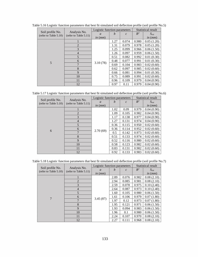
133
Table 5.16 Logistic function parameters that best fit simulated soil deflection profile (soil profile No.5)
Soil profile No. (refer to Table 5.10)
Analysis No. (refer to Table 5.11)
Logistic function parameters Statistical result
a
in (mm)
b
c
R2
Sest
in (mm)
5
1
3.10 (78)
1.27 0.074 0.980 0.05 (1.20)
2 1.31 0.079 0.978 0.05 (1.20)
3 1.25 0.099 0.966 0.06 (1.50)
4 1.26 0.097 0.959 0.06 (1.50)
5 0.51 0.082 0.992 0.01 (0.30)
6 0.48 0.077 0.991 0.01 (0.30)
7 0.69 0.104 0.983 0.02 (0.60)
8 0.62 0.097 0.985 0.02 (0.60)
9 0.66 0.081 0.994 0.01 (0.30)
10 0.75 0.089 0.991 0.02 (0.60)
11 0.96 0.109 0.979 0.04 (0.90)
12 0.97 0.11 0.979 0.04 (0.90)
Table 5.17 Logistic function parameters that best fit simulated soil deflection profile (soil profile No.6)
Soil profile No. (refer to Table 5.10)
Analysis No. (refer to Table 5.11)
Logistic function parameters Statistical result
a
in (mm)
b
c
R2
Sest
in (mm)
6
1
2.70 (69)
1.02 0.09 0.979 0.04 (0.90)
2 1.09 0.105 0.982 0.04 (0.90)
3 1.17 0.138 0.977 0.04 (0.90)
4 1.27 0.131 0.974 0.04 (0.90)
5 0.36 0.115 0.950 0.02 (0.60)
6 0.36 0.114 0.952 0.02 (0.60)
7 0.5 0.142 0.973 0.02 (0.60)
8 0.51 0.133 0.974 0.02 (0.60)
9 0.52 0.116 0.980 0.02 (0.60)
10 0.58 0.123 0.982 0.02 (0.60)
11 0.83 0.131 0.982 0.02 (0.60)
12 0.92 0.133 0.983 0.02 (0.60)
Table 5.18 Logistic function parameters that best fit simulated soil deflection profile (soil profile No.7)
Soil profile No. (refer to Table 5.10)
Analysis No. (refer to Table 5.11)
Logistic function parameters Statistical result
a
in (mm)
b
c
R2
Sest
in (mm)
7
1
3.45 (87)
2.89 0.076 0.982 0.08 (2.10)
2 2.94 0.085 0.981 0.08 (2.10)
3 2.59 0.078 0.975 0.10 (2.40)
4 2.64 0.087 0.973 0.10 (2.40)
5 1.60 0.105 0.980 0.06 (1.50)
6 1.61 0.106 0.979 0.07 (1.80)
7 1.97 0.12 0.973 0.07 (1.80)
8 1.95 0.121 0.971 0.06 (1.50)
9 1.93 0.094 0.983 0.06 (1.50)
10 1.96 0.1 0.980 0.06 (1.50)
11 2.24 0.107 0.970 0.08 (2.10)
12 2.27 0.111 0.968 0.08 (2.10)

134
Table 5.19 Logistic function parameters that best fit simulated soil deflection profile (soil profile No.8)
Soil profile No. (refer to Table 5.10)
Analysis No. (refer to Table 5.11)
Logistic function parameters Statistical result
a
in (mm)
b
c
R2
Sest
in (mm)
8
1
2.20 (55)
2.01 0.089 0.981 0.04 (0.90)
2 2.1 0.093 0.980 0.04 (0.90)
3 1.98 0.103 0.966 0.05 (1.20)
4 2.02 0.102 0.966 0.05 (1.20)
5 1.19 0.122 0.988 0.02 (0.60)
6 1.17 0.122 0.988 0.02 (0.60)
7 1.37 0.133 0.986 0.02 (0.60)
8 1.35 0.133 0.985 0.02 (0.60)
9 1.19 0.092 0.992 0.01 (0.30)
10 1.21 0.094 0.991 0.01 (0.30)
11 1.64 0.119 0.981 0.04 (0.90)
12 1.65 0.119 0.981 0.04 (0.90)
Table 5.20 Logistic function parameters that best fit simulated soil deflection profile (soil profile No.9)
Soil profile No. (refer to Table 5.10)
Analysis No. (refer to Table 5.11)
Logistic function parameters Statistical result
a
in (mm)
b
c
R2
Sest
in (mm)
9
1
2.10 (52)
1.82 0.103 0.982 0.04 (0.90)
2 1.91 0.108 0.979 0.04 (0.90)
3 1.94 0.128 0.967 0.05 (1.20)
4 1.94 0.125 0.963 0.05 (1.20)
5 0.82 0.108 0.990 0.01 (0.30)
6 0.77 0.103 0.991 0.01 (0.30)
7 0.94 0.119 0.986 0.01 (0.30)
8 0.93 0.118 0.987 0.01 (0.30)
9 1.1 0.106 0.993 0.01 (0.30)
10 0.94 0.095 0.991 0.01 (0.30)
11 1.42 0.131 0.981 0.02 (0.60)
12 1.45 0.131 0.980 0.02 (0.60)
5.9 Evaluating logistic function parameters
The next step would be to evaluate each of the logistic function parameters (a, b, and c)
individually to see if they can be determined using geometric and soil parameters. For this
purpose, correlation and regression analysis were carried out.
First, a correlation analysis was conducted to examine the relationship among the logistic
function parameters. Table 5.21 shows the result of this study. Accordingly, the result indicate
that the three parameters are not correlated with each other, except for parameters (a) and (c) for
which a strong negative correlation exists.

135
Table 5.21 Pearson’s correlation coefficient among logistic function parameters
Parameter a b c
a 1.00 0.170 -0.830
b 0.170 1.00 -0.083
c -0.830 -0.083 1.00
Subsequently, another analysis was carried out to examine the correlation between
parameters a, b, and c with fundamental soil properties (backfill soil, embankment soil, and
natural soil), as well as geometric parameters. In this analysis, a was decomposed into two
components; ultimate settlement resulting from the natural soil an, and ultimate settlement
resulting from the embankment fill ae, in which (a = an + ae). This was to examine the
contribution of each soil layer to the total surface settlement a. Table 5.22 shows the
decomposition of the simulated ultimate settlement a.
Table 5.22 Decomposition of the simulated ultimate settlement a
Soil profile No. (refer to Table 5.10)
a
in (mm)
an
in (mm)
ae
in (mm)
1 8.20 (208) 5.50 (141) 2.70 (67)
2 6.30 (159) 4.90 (124) 1.40 (35)
3 5.10 (129) 3.90 (98) 1.20 (31)
4 3.60 (91) 2.20 (55) 1.40 (36)
5 3.10 (78) 1.80 (47) 1.30 (31)
6 2.70 (69) 1.50 (37) 1.20 (32)
7 3.45 (87) 1.90 (48) 1.55 (39)
8 2.20 (55) 1.70 (44) 0.50 (11)
9 2.10 (52) 1.50 (37) 0.60 (15)
Table 5.23 shows the result of the correlation study between the logistic function
parameters and backfill soil properties. Table 5.24 shows the result of the correlation study
between the logistic function parameters and embankment soil properties. Table 5.25 shows the
result of the correlation study between the logistic function parameters and natural soil
properties. Table 5.26 shows the result of the correlation study between the logistic function
parameters and geometric parameters.

136
Table 5.23 Pearson’s correlation coefficient between logistic function parameters and backfill soil properties
Soil properties a an ae b c
φ' 0.000 0.000 0.000 -0.133 -0.211
ɣ 0.000 0.000 0.000 -0.125 -0.233
e0 0.000 0.000 0.000 -0.125 -0.233
E 0.000 0.000 0.000 0.125 0.233
Table 5.24 Pearson’s correlation coefficient between logistic function parameters and embankment soil properties
Soil properties a an ae b c
C' -0.443 -0.393 -0.471 -0.651 0.309
φ' -0.435 -0.389 -0.453 -0.643 0.307
ɣ 0.475 0.406 0.545 0.682 -0.312
ѵ 0.384 0.362 0.355 0.588 -0.294
Cc 0.472 0.405 0.537 0.720 -0.312
Cs 0.486 0.409 0.572 0.691 -0.312
e0 0.476 0.406 0.547 0.683 -0.312
E -0.497 -0.410 -0.606 -0.699 0.309
Table 5.25 Pearson’s correlation coefficient between logistic function parameters and natural soil properties
Soil properties a an ae b c
C' -0.307 -0.388 -0.039 -0.461 0.492
φ' -0.355 -0.455 -0.026 -0.500 0.430
ɣ -0.276 -0.361 0.000 -0.352 0.184
ѵ 0.247 0.307 0.041 0.388 -0.471
Cc 0.354 0.455 0.024 0.495 -0.413
Cs 0.354 0.455 0.024 0.495 -0.413
e0 0.354 0.455 0.024 0.495 -0.414
E -0.350 -0.447 -0.031 -0.503 0.464
Table 5.26 Correlation coefficient between logistic function parameters and geometric parameters
Geometric parameters a an ae b c
He 0.548 0.509 0.525 -0.526 -0.458
Ha 0.000 0.000 0.000 0.460 -0.211
Sb 0.000 0.000 0.000 0.011 0.016
Ha / He 0.145 -0.135 -0.139 0.622 -0.082
5.9.1 Logistic function parameter (a)
As shown in Tables 5.23, 5.24 and 5.25, parameter a does not have a strong correlation
with the backfill soil properties. Nevertheless, stronger correlation exists between a and the
embankment fill as well as natural soil fundamental properties. Therefore, the problem can be
further simplified to include only the embankment fill and natural soil layers. This was done by
considering a vertical soil strip (along the longitudinal-direction) with a unit longitudinal length

137
that includes the pavement roadway (as a pressure), embankment fill layer, and natural soil layer,
as shown in Figure 5.75.
Figure 5.75 Calculation of (a) using a vertical strip (longitudinal-direction)
In general, the weight of any soil layer or structure will impose stresses on the underlying
soil layers. These stresses will eventually cause dimensional changes in the soil volume
(decrease in the volume) through which settlement of soil occurs. This settlement can be
expressed by the summation of three separate components; the initial settlement (reduction of
void ratio), primary settlement (dissipation of water), and secondary settlement (creep).
According to the MDPCM model, this settlement can be expressed in terms of total strain.
Therefore, the ultimate settlement can be represented by the volumetric elastic and plastic strains
developed within the soil layer. Accordingly, it was assumed that the deformation of the soil
away from the abutment takes place only in the vertical direction. Such an assumption would
allow explaining the settlement of each soil layer by its elastic and plastic volumetric
deformation. Ultimately, the total volumetric strain can be expressed as:

138
𝑑𝜀𝑣 = 𝑑𝜀𝑣𝑒 + 𝑑𝜀𝑣
𝑝 5-5
The total volumetric strain can be evaluated individually for each soil layer. This was
done by further simplifying the problem into two separate parts (presented in Figure 5.75):
settlement of the embankment fill due to the weight of the roadway pressure ae and settlement of
the natural soil due to the weight of the embankment fill an, as shown in Figure 5.76.
Figure 5.76 Calculation of (a) ae and (b) an
The volumetric elastic deformation of soil can be conveniently represented by a linear
elastic deformation using Hooke’s law as follows:
𝜀𝑣
𝑒 =𝜎0 + ∆𝜎
𝐸 5-6
Where, 𝜎0, ∆𝜎, 𝐸 are the in-situ pressure, surcharge pressure, and modulus of elasticity of
soil, respectively. The volumetric elastic strain can be adjusted to accommodate for the nonlinear
behavior of the soil (within the elastic region). This is particularly the case with the over-
consolidated soils, where a nonlinear deformation based on over-consolidation ratio (OCR) is
expected. Therefore, an overburden stress ratio term (increase of the stress ratio) (𝜎0+∆𝜎
𝜎0) can be
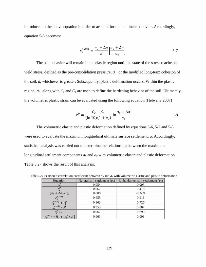
139
introduced in the above equation in order to account for the nonlinear behavior. Accordingly,
equation 5-6 becomes:
𝜀𝑣
𝑒.𝑎𝑑𝑗=
𝜎0 + ∆𝜎
𝐸[𝜎0 + ∆𝜎
𝜎0] 5-7
The soil behavior will remain in the elastic region until the state of the stress reaches the
yield stress, defined as the pre-consolidation pressure, 𝜎𝑐, or the modified long-term cohesion of
the soil, d, whichever is greater. Subsequently, plastic deformation occurs. Within the plastic
region, 𝜎𝑐, along with Cs and Cc are used to define the hardening behavior of the soil. Ultimately,
the volumetric plastic strain can be evaluated using the following equation (Helwany 2007)
𝜀𝑣
𝑝 =𝐶𝑐 − 𝐶𝑠
(ln 10)(1 + 𝑒0) ln
𝜎0 + ∆𝜎
𝜎𝑐 5-8
The volumetric elastic and plastic deformation defined by equations 5-6, 5-7 and 5-8
were used to evaluate the maximum longitudinal ultimate surface settlement, a. Accordingly,
statistical analysis was carried out to determine the relationship between the maximum
longitudinal settlement components an and ae with volumetric elastic and plastic deformation.
Table 5.27 shows the result of this analysis.
Table 5.27 Pearson’s correlation coefficient between an and ae with volumetric elastic and plastic deformation
Equation Natural soil settlement (an) Embankment soil settlement (ae)
𝜀𝑣𝑒 0.954 0.903
𝜀𝑣𝑝 0.967 0.418
(𝜎0 + ∆𝜎) 𝜎0⁄ 0.808 -0.669
𝜀𝑣𝑒.𝑎𝑑𝑗
0.955 0.911
𝜀𝑣𝑒.𝑎𝑑𝑗
+ 𝜀𝑣𝑝 0.963 0.726
𝜀𝑣𝑒.𝑎𝑑𝑗
∗ 𝐻 0.953 0.807
𝜀𝑣𝑝
∗ 𝐻 0.967 0.693
[𝜀𝑣𝑒.𝑎𝑑𝑗
∗ 𝐻] + [𝜀𝑣𝑝
∗ 𝐻] 0.963 0.901

140
As shown in the above table, a very strong correlation exists between the total strain
(𝜀𝑣𝑒.𝑎𝑑𝑗
+ 𝜀𝑣𝑝) and the simulated settlement components ae and an. Accordingly, scatter plots,
shown in Figures 5.77 and 5.78, were constructed to examine the relationship between them.
Figure 5.77 Scatter plot between total volumetric strain and settlement component (ae)
0
25
50
75
100
0
1
2
3
4
0.0 0.1 0.2 0.3 0.4 0.5 0.6 0.7 0.8
(ae)
(m
m)
(ae)
(in
)
Total volumetric strain
Relationship between total volumetric strain and (ae)
Simulated data
Polynomial model (2nd degree)
Exponential model

141
Figure 5.78 Scatter plot between total volumetric strain and settlement component (an)
Various trials were made, using curve fitting software (curve expert), to find the best fit
curve between the simulated ultimate soil components and the total volumetric strain. The best
fit curves are shown in the above figures. It is concluded that the relationship between
(𝜀𝑣𝑒.𝑎𝑑𝑗
+ 𝜀𝑣𝑝) and ae may be represented by an exponential function. Similar observation was
made for the relationship between (𝜀𝑣𝑒.𝑎𝑑𝑗
+ 𝜀𝑣𝑝) and an. Therefore, an exponential relationship
could be proposed as follows:
𝑎𝑛 = 𝐶𝑛𝐻𝑛𝑒(𝛽𝑛𝜀𝑣
𝑒.𝑎𝑑𝑗+𝛼𝑛𝜀𝑣
𝑝) 5-9
𝑎𝑒 = 𝐶𝑒𝐻𝑒𝑒(𝛽𝑒𝜀𝑣
𝑒.𝑎𝑑𝑗+𝛼𝑒𝜀𝑣
𝑝) 5-10
In which,
0
25
50
75
100
0
1
2
3
4
5
6
7
8
0 1 2 3 4
(an)
(mm
)
(an)
(in)
Total volumetric strain
Relationship between total volumetric strain and (an)
Simulated data
Polynomial model (2nd degree)
Exponential model

142
𝑎 = 𝑎𝑛 + 𝑎𝑒 5-11
and
a = Ultimate settlement at the top surface of the embankment fill.
an = Settlement component at the top surface of the natural soil.
ae = Settlement component at the top surface of the embankment fill.
Hn = Height of the natural soil layer.
He = Height of the embankment fill.
Ce, Cn, βn, βe, αn and αe = Regression parameters.
Accordingly, a regression analysis was conducted using the method of least squares in
order to determine the best fit for the exponential relationships proposed above. Table 5.28
shows the results for the regression parameters Ce, Cn, βn, αn, βe and αe.
Table 5.28 Regression parameters of the ultimate settlement components (an) and (ae).
Parameter Value
𝐶𝑛 383×10-6
𝛽𝑛 27.00
𝛼𝑛 38.60
𝐶𝑒 4980×10-6
𝛽𝑒 61.00
𝛼𝑒 23.00
The final equation was evaluated by substituting the value of various parameters (found
in Table 5.28) into equations 5-9, 5-10. Thus, the maximum longitudinal surface settlement, a,
can be evaluated using the following equation
𝑎 = 383 × 10−6𝐻𝑛𝑒(27 𝜀𝑣𝑒.𝑎𝑑𝑗
+38.6 𝜀𝑣𝑝
) + 4980 × 10−6𝐻𝑒𝑒(61 𝜀𝑣𝑒.𝑎𝑑𝑗
+23 𝜀𝑣𝑝
) 5-12
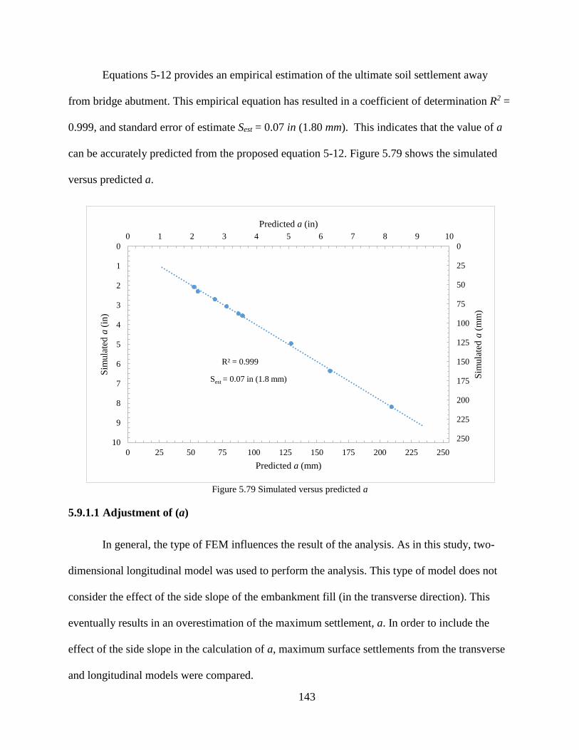
143
Equations 5-12 provides an empirical estimation of the ultimate soil settlement away
from bridge abutment. This empirical equation has resulted in a coefficient of determination R2 =
0.999, and standard error of estimate Sest = 0.07 in (1.80 mm). This indicates that the value of a
can be accurately predicted from the proposed equation 5-12. Figure 5.79 shows the simulated
versus predicted a.
Figure 5.79 Simulated versus predicted a
5.9.1.1 Adjustment of (a)
In general, the type of FEM influences the result of the analysis. As in this study, two-
dimensional longitudinal model was used to perform the analysis. This type of model does not
consider the effect of the side slope of the embankment fill (in the transverse direction). This
eventually results in an overestimation of the maximum settlement, a. In order to include the
effect of the side slope in the calculation of a, maximum surface settlements from the transverse
and longitudinal models were compared.
Sest = 0.07 in (1.8 mm)
R² = 0.999
0 25 50 75 100 125 150 175 200 225 250
0
25
50
75
100
125
150
175
200
225
250
0
1
2
3
4
5
6
7
8
9
10
0 1 2 3 4 5 6 7 8 9 10
Predicted a (mm)
Sim
ula
ted
a(m
m)
Sim
ula
ted
a(i
n)
Predicted a (in)

144
In this analysis, all soil profiles (shown in Table 5.10) were tested. The analysis was
carried out such that the side slope of the embankment fill, oriented in the transverse direction,
was straightened up, by adding more filling material (A3 in Figure 5.80). The maximum surface
settlements of the sloped and straightened embankment fills were compared with the maximum
longitudinal surface settlement, a.
Figure 5.80 Layout of the transverse simulation (additional fill)
Figures 5.81 through 5.83 show the result of the analysis using soil profile No.1 (see
Table 5.10).

145
Figure 5.81 Vertical deformation contour (transverse direction) of soil profile No.1 (ft)
Figure 5.82 Vertical deformation contour (transverse direction) of soil profile No.1 with additional fill (ft)
Figure 5.83 Vertical deformation contour (longitudinal direction) of soil profile No.1 (analysis#3) (ft)
The above figures show that the anticipated maximum surface settlement from the
transverse model (Figure 5.81) was less than the longitudinal model (Figure 5.83). Figure 5.82
shows that after adding more fill, the surface settlement at the center of the embankment has
increased to relatively match the maximum longitudinal settlement, a. Similar observation was
found with all tested soil profiles. Accordingly, a relationship was sought by relating the area
ratio of embankment fill to the maximum longitudinal settlement, a. Ultimately, the difference in
the filling area was assumed to be proportional with a as follows:

146
𝑎𝑎𝑑𝑗 = 𝑎 (1 −
𝐴3
𝐴1 + 𝐴2) 5-13
Where
A1 + A2 = Total transverse area of the embankment fill (see Figure 5.80)
A3 = Transverse area of the additional fill (see Figure 5.80).
Accordingly, regression analysis was conducted using the method of least squares to
determine the best fit for the latter relationship. Consequently, the final equation was evaluated
as follows:
𝑎𝑎𝑑𝑗 = 0.92𝑎 (1 −
𝐴3
𝐴1 + 𝐴2) + 0.82 5-14
Equation 5-14 provides an empirical relationship that relates the maximum longitudinal
settlement, a, with the maximum transverse surface settlement. Figure 5.84 shows the simulated
versus predicted a using equation 5-14.

147
Figure 5.84 Simulated versus predicted (a)
5.9.2 Logistic function parameter (b)
As shown in Tables 5.24 and 5.26, parameter (b) has a strong correlation with the
embankment soil properties as well as the geometric parameters. They include embankment
compression index (Cc) (r = 0.720) and the abutment to embankment height ratio (He / Ha) (r =
0.622). Accordingly, it was observed that the correlation coefficient increases to (r = 0.808) as a
result of multiplying the embankment compression index with the abutment to embankment
height ratio (i.e. Cc × Ha / He). Thus, a scatter plot, shown in Figure 5.85, was constructed
between parameter (b) and (Cc × Ha / He).
Sest = 0.16 in (4 mm)
R² = 0.9872
0 25 50 75 100 125 150 175
0
25
50
75
100
125
150
175
0
1
2
3
4
5
6
7
8
9
0 1 2 3 4 5 6 7
Predicted a (mm)
Sim
ula
ted
a(L
ongit
ud
inal
) (m
m)
Sim
ula
ted
a(L
ongit
ud
inal
) (i
n)
Predicted a (in)

148
Figure 5.85 Scatter Plot between parameter (b) and (Cc × Ha / He)
Various trials were made, using curve fitting software (curve expert), to find the best fit
curve between the logistic function parameter, b, with (Cc × Ha / He). The best fit curves are
shown in the above figures. It is concluded that the relationship between parameter b and (Cc ×
Ha / He) may be best represented by a logarithmic function as shown below:
𝑏 = ϑ 𝑙𝑛 (𝐶𝑐 ×
𝐻𝑎
𝐻𝑒) + Ѱ 5-15
Where
Cc = Compression index of the embankment fill.
He = Height of the embankment fill.
Ha = Height of the abutment wall.
ϑ and Ѱ = Regression parameters.
0
1
2
3
0 0.1 0.2 0.3 0.4 0.5 0.6 0.7
(b)
Cc × (Ha / He)
Relationship between (b) and (Cc × Ha / He)
Simulated data
Polynomial model (2nd degree)
Logarithmic model

149
Consequently, a regression analysis was conducted using the method of least squares in
order to determine the best fit parameters for the logarithmic relationship. Table 5.29 shows the
results for the regression parameters ϑ and Ѱ.
Table 5.29 Regression parameters of the logarithmic function
Parameter Value
ϑ 0.38
Ѱ 2.26
The final equation was evaluated by substituting the parameters value (found in Table
5.29) into equation 5-15 as follows:
𝑏 = 0.38 𝑙𝑛 (𝐶𝑐 ×
𝐻𝑎
𝐻𝑒) + 2.26 5-16
Equation 5-16 provides an empirical estimation for the parameter b, which controls the
magnitude of the settlement at the interface between the abutment wall and adjacent soil. This
empirical equation resulted in a coefficient of determination R2 = 0.794, and standard error of
estimate Sest = 0.15. This indicates that the value of b can be predicted reasonably well using
equation 5-16. Figure 5.86 shows the simulated versus predicted b.

150
Figure 5.86 Simulated versus predicted b
5.9.3 Logistic function parameter (c)
As shown in Table 5.21, a very strong negative correlation exists between parameters a
and c, with a value of (r = -0.830). Figure 5.87 shows a scatter plot between parameter a and c.
Sest = 0.15
R² = 0.7939
0
0.5
1
1.5
2
2.5
0 0.5 1 1.5 2 2.5 3S
imula
ted
b
Predicted b

151
Figure 5.87 Scatter plot between parameter a and c
Various trials were made, using curve fitting software (curve expert), to find the best fit
curve of the logistic function parameter, c. The best fit curves are shown in the above figures. It
is concluded that the relationship between c and a may follow an exponential function.
Therefore, an exponential function could be proposed as follows:
𝑐 = ηeω𝑎 5-17
Where
η and ω = Regression parameters.
Accordingly, a regression analysis was conducted using the method of least squares in
order to determine the best fit for the exponential relationship. Table 5.30 shows the results for
the parameters η and ω.
0 25 50 75 100 125 150 175 200 225 250
0
0.05
0.1
0.15
0.2
0 1 2 3 4 5 6 7 8 9 10
a (mm)c
a (in)
Relationship between a and c
Simulated data
Polynomial model (2nd degree)
Exponential model
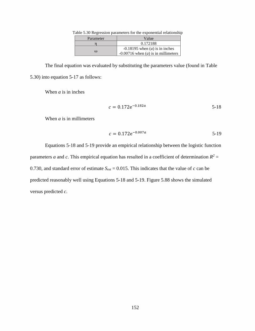
152
Table 5.30 Regression parameters for the exponential relationship
Parameter Value
η 0.172188
ω -0.18195 when (a) is in inches
-0.00716 when (a) is in millimeters
The final equation was evaluated by substituting the parameters value (found in Table
5.30) into equation 5-17 as follows:
When a is in inches
𝑐 = 0.172e−0.182𝑎 5-18
When a is in millimeters
𝑐 = 0.172e−0.007𝑎 5-19
Equations 5-18 and 5-19 provide an empirical relationship between the logistic function
parameters a and c. This empirical equation has resulted in a coefficient of determination R2 =
0.730, and standard error of estimate Sest = 0.015. This indicates that the value of c can be
predicted reasonably well using Equations 5-18 and 5-19. Figure 5.88 shows the simulated
versus predicted c.

153
Figure 5.88 Simulated versus predicted c
5.10 Case study
A case study was considered and examined, using the finite element method, to
investigate the accuracy of the developed empirical equations with respect to estimating the
longitudinal soil deflection profile behind bridge abutment.
The soil profile used in the case study is similar to that shown in Figure 5.33. It consisted
of a wall abutment with height Ha = He constructed against a 95% compacted granular backfill
with Sb = 1:2 (1 vertical to 2 horizontal), low compressible embankment fill with height He = 25
ft (7.6 m) and moderate compressible natural soil with height Hn = 35 ft (10.7 m). The material
properties associated with the concrete in the abutment wall, approach slab, and roadway
pavement as well as soil properties are shown in Tables 4.2 and 4.7, respectively.
Sest = 0.015
R² = 0.730
0
0.02
0.04
0.06
0.08
0.1
0.12
0.14
0 0.02 0.04 0.06 0.08 0.1 0.12 0.14S
imula
ted
c
Predicted c

154
The boundary conditions, analysis steps, elements type, and contact behavior were
described in section 5.6. Figure 5.89 shows the finite element discretization of the case study
model.
Figure 5.89 Finite element discretization of the case study model
Results from the finite element analysis of are presented in Figures 5.90, 5.91 and 5.92.
Figure 5.90 shows the vertical deformation of the abutment, approach slab, roadway,
embankment fill, and natural soil at the end of the analysis. Figure 5.91 shows the distribution of
excess pore pressure at the end of the analysis. Figure 5.92 shows the simulated soil deformation
profile along the longitudinal direction.
Figure 5.90 Deformed mesh at the end of the analysis (ft)

155
Figure 5.91 Distribution of excess pore pressure at the end of the analysis (psf)
Figure 5.92 Simulated versus predicted soil settlement profile for the case study
Figure 5.92 indicates that the far away settlement, a, and settlement adjacent to abutment
wall were 2.6 in (66 mm) and 0.4 in (10 mm), respectively. The developed logistic empirical
function (equation 5-3) was used to predict the longitudinal soil deformation profile. First,
equation 5-12 was used to determine the value of the ultimate settlement far away from bridge
0 10 20 30 40 50 60
0
25
50
75
0
1
2
3
0 20 40 60 80 100 120 140 160 180 200
Distance away from the bridge (m)
Ver
tica
l se
ttle
men
t (m
m)
Ver
tica
l se
ttle
men
t (i
n)
Distance away from the bridge (ft)
Soil settlement profile behind bridge abutment
Simulated soil profile
Predicted soil profile

156
abutment, a. The developed level of strain was individually evaluated for embankment fill and
natural soil layers. Table 5.31 shows the level of strain at the middle of each layer.
Table 5.31 Level of strain at the middle of each layer
Strain Embankment Fill Natural Soil
𝜀𝑣𝑒.𝑎𝑑𝑗
0.0048 0.0225
𝜀𝑣𝑝 0 0.016
Substituting the values of 𝜀𝑣𝑒.𝑎𝑑𝑗
and 𝜀𝑣𝑝 into equation 5-12, a yields to 2.5 in (64 mm).
Subsequently, substituting Cc = 0.087, He = 25 ft (7.6 m), and Hn = 35 ft (10.7 m) into equation
5-16, b yields to 1.53. Lastly, substituting a = 2.5 in into equation 5-18 yields to c = 0.11. Figure
5.92 shows the simulated versus predicted soil profiles. The figure shows that the developed
logistic function predicted the soil deformation along the longitudinal direction reasonably well
when compared with the finite element results.
5.11 Chapter summary and conclusion
The objective of this study was to provide engineers with a reasonably accurate, yet
simple, empirical equations that could be used to predict the longitudinal soil deformation behind
bridge abutments. Such equations would be beneficial in making reliable predictions of the long-
term differential settlement of the approach slab and could facilitate more accurate design
recommendations to address bridge approach settlements.
Parametric studies were conducted, using finite element model, to quantify the effects of
various parameters on the transverse as well as longitudinal soil deflection profile behind bridge
abutments. These include the length of the approach slab, height of embankment fill,
embankment soil type, height of natural soil, natural soil type, backfill soil type, slope of backfill
area, and abutment type.

157
As a result, it can be concluded that embankment fill height of He > 20 ft ( 6.1 m) would
be problematic in terms of the transition performance. The slope of the approach slab must be
checked against soil conditions in such cases. In addition, it was observed that the soil
longitudinal deflection profile could be represented by a logistic function curve. Therefore, a set
of empirical equations were developed that define the various parameters of the logistic function.
Table 5.32 shows a summary of the developed equations.
Table 5.32 Summary of the developed equation
General form/parameters Developed equations
General form of the
logistic function
y = vertical settlement at a
distance of x from the
bridge abutment.
y =𝑎
1 + 𝑏𝑒−𝑐𝑥
Logistic function
parameter (a)
Maximum displacement. 𝑎 = 383 × 10−6𝐻𝑛𝑒(27 𝜀𝑣
𝑒.𝑎𝑑𝑗+38.6 𝜀𝑣
𝑝) + 4980 × 10−6𝐻𝑒𝑒(61 𝜀𝑣
𝑒.𝑎𝑑𝑗.+23 𝜀𝑣
𝑝)
Logistic function
parameter (b)
Settlement at the interface
between the abutment wall
and the backfill soil.
𝑏 = 0.38 𝑙𝑛 (𝐶𝑐 ×𝐻𝑒
𝐻𝑎
) + 2.26
Logistic function
parameter (c)
Steepness of the curve.
𝑐 = 0.172e−0.182𝑎 *
𝑐 = 0.172e−0.007𝑎 **
* when (a) is in inches ** when (a) is in millimeters
The range of applicability of the developed equations would typically be restricted to the
range of the parameters used in the parametric study (see Tables 5.9, 5.10 and 5.11). Care must
be taken to ensure accuracy if parameters are outside of the range used in the parametric study. A
particular case was illustrated in which the developed equations predicted the simulated soil
deformation reasonably well. Overall, the benefits of the developed equations could be further
increased when studies using an expanded range of parameters are conducted in the future.

158
CHAPTER 6 - PILE-SUPPORTED APPROACH SLABS
6.1 Chapter background
As soil underneath approach slab settles, deferential settlement develops between the
bridge and the roadway pavement causing bumps and affecting the riding quality. The approach
slab in such cases would transfer the bump from the beginning of the bridge to the end of the
approach slab. As discussed in the literature review chapter (Chapter 2), a maximum change of
slope of approach slab of 1/125 is desired to maintain a smooth transition into and out of the
bridge. Maintaining such limits in slope is important to prevent damage to structural elements, to
ensure safe driving environment, and to reduce maintenance cost over the life-time of the bridge
system.
Figure 6.1 Managing approach slab differential settlement
Settlement-reducing piles could be introduced into the approach slab to control changes
in slope and limit stresses to acceptable levels. Such piles would rely on surface friction and end-
bearing resistant to control the approach slab settlement and achieve the required level of
differential settlement. However, determining the appropriate location, spacing, length and size

159
of piles is a difficult task that requires further study. Since field testing of piles is rather
expensive and time-consuming, an analytical program (which is verified with through existing
test information) is required to develop the information needed for the design of pile supported
approach slab for settlement control.
6.2 Chapter problem statement
Since the bridge approach slab (BAS) is a relatively rigid structural member, a smooth
transition (change in slope of less than 1/125) may be achieved by selecting the length of the
approach slab, LBAS, such that the resulting slope is acceptable for the expected soil settlement.
However, when the soil conditions are poor, the soil settlement would be large, and the approach
slab must be extended far to bridge the gap resulting from the settlement. This could in return
result in very long approach slabs that would require greater thicknesses to control stresses and
deflection. Introducing piles at specific locations underneath a segmented approach slab could
address such a problem through control of soil settlement and slope changes. As piles are
introduced, they could control downward movement of the soil to acceptable levels by offering
resistance to the soil (downdrag). Control of settlements along various segments of a multi-
segment approach slab could facilitate slope changes that within tolerable limits with respect of
ride quality. Piles in such cases are not intended to reduce settlement to zero as this would only
add another apparent span to the bridge and would not address the differential settlement that
must still be accommodated.
Maintaining acceptable slope changes among approach slab segment and between
approach slab segments and the roadway or the bridge is required to achieve an overall smooth
transition between the bridge and the roadway pavement. The concept of pile supported
segmented approach slab is illustrated in Figure 6.1. The approach slab segments are attached

160
together in such a way as to allow rotation at the interface between segments thus allowing a
series of changes in slope. The number and lengths of needed approach slab segments are
dependent on the expected settlement. One approach involves developing an S-shaped curve to
eliminate the formation of the bump. The S curve would require an odd number of segments in
which the settlement at the end of each segment is controlled through piles. The characteristics of
each segment can be determined based on the desired relative angle change between any two
segments. Figure 6.2 shows a schematic of the proposed multi-segment pile supported approach
slab.
Figure 6.2 Schematic of the proposed pile supported approach slab segments.
For the purposes of this study, the length of each approach slab segment is assumed to be
between 15 ft (4.5 m) and 30 ft (9.1 m), which are compatible with typical lengths used for
approach slab (see Chapter 3). In order to produce the smooth transition curve shown in Figure
161
6.2, the change of the slope between the bridge and the first segment, 𝜑𝐴, should be maintained
at a level below the 1/125. Similarly, the change of slope at the second and third segments, ∆𝜑𝐵
and ∆𝜑𝐶, should be less than the targeted value as well. Additionally, while maintaining the
limits on slope change, the middle segment can have an absolute slope that can be as much as
twice the slope change limit. This indicates that BAS-B can undergo twice the differential
settlement of the first and third segments, i.e. ∆𝐵= 2∆𝐴. This would shorten the overall length of
the three-segment approach slab compared to a single-segment regular approach slab. Such a
pile-supported multi-segment approach slab is expected to result in a smooth transition between
the bridge and the roadway in cases where excessive soil settlement is expected.
In some circumstances, fewer (two) approach slab segments maybe adequate for
achieving slope changes that are below the stated limits. In such cases, the procedures described
below can be followed. Eventually, the produced smooth curve would consist of one or more
approach slab segments that serves the purpose of eliminating the bump at the end of the bridge.
The procedures used to produce the smooth curve transition is as follows: (refer to Figure 6.2)
a) Determine the maximum longitudinal surface soil settlement, a or ∆𝑇, using either the
FEM analysis or the empirical equations provided in Chapter 5.
b) If ∆𝑇≤ 𝐿𝐵𝐴𝑆−𝐴 (1
125), use a single-segment approach slab with 𝐿𝐵𝐴𝑆−𝐴 ≤
30𝑓𝑡 (9.1𝑚). Minimize 𝐿𝐵𝐴𝑆−𝐴 to meet this requirement.
c) If ∆𝑇> 𝐿𝐵𝐴𝑆−𝐴 (1
125), the settlement cannot be accommodated with a single-segment
approach slab. Use a multi-segment pile-supported approach slab based on the
following procedures:

162
a. Select pile size, length, and pile spacing for the first line of piles such that the
expected pile head settlement ∆𝐴≤ 𝐿𝐵𝐴𝑆−𝐴 (1
125). Charts that can be used for
this estimation are given in this Chapter. If the desired ∆𝐴 cannot be achieved,
change 𝐿𝐵𝐴𝑆−𝐴, pile size, pile length, or pile spacing to satisfy the above
settlement requirement.
b. If 𝐿𝐵𝐴𝑆−𝐴 (1
125) < ∆𝑇≤ (𝐿𝐵𝐴𝑆−𝐴 + 𝐿𝐵𝐴𝑆−𝐵) (
1
125), try a two-segment
approach slab with one line of piles between the two segments. The end of the
second segment should be supported on a sleeper-slab on soil.
c. If ∆𝑇> (𝐿𝐵𝐴𝑆−𝐴 + 𝐿𝐵𝐴𝑆−𝐵) (1
125), the settlement cannot be accommodated
with a two-segment approach slab. Try a three-segment approach slab. The
end of the third segment should be supported on a sleeper-slab on soil.
d. Select the pile size, length, and pile spacing for the second line of piles (from
the charts) such that the expected pile head settlement ∆𝐴 + ∆𝐵≤
(𝐿𝐵𝐴𝑆−𝐴 + 𝐿𝐵𝐴𝑆−𝐵) (1
125).
e. If ∆𝑇> (𝐿𝐵𝐴𝑆−𝐴 + 2𝐿𝐵𝐴𝑆−𝐵 + 𝐿𝐵𝐴𝑆−𝐶) (1
125), the settlement cannot be
accommodated with a three-segment approach slab. Try four-segment
approach slab. The end of the fourth segment could be supported on a sleeper-
slab on soil.
f. Repeat steps a-e as needed.

163
6.3 Chapter objectives
The objective of this phase of the study is to quantify the effects of the pile, soil and
bridge parameters on the pile head settlement. Relationships are required for estimating pile head
settlement under various pile and soil conditions. These relationships can be utilized to determine
the appropriate location, size, length, and spacing of piles to achieve and maintain a smooth
transition between the bridge and roadway pavement in cases of excessive settlement.
6.4 Settlement-reducing piles
6.4.1 Introduction
Piles are long slender structural members that are commonly made of concrete, steel, or
timber and are used to transfer superstructure loads deep into the soil. Their main function is to
provide adequate bearing capacity to resist applied load. However, piles can also be used to
reduce settlement to an acceptable level. Piles are typically installed in group of three or more to
insure safe load transfer and provide some redundancy to the supported structure/s. There are
two basic types of pile foundations; friction pile and end-bearing pile. A friction pile derives its
capacity through skin friction, Qs, that is developed over the surface of the pile. On the other
hand, the end-bearing pile derives its capacity, Qb, from the bearing capacity of the soil under the
pile tip. A combination of the two pile types (semi-friction pile) provides resistance through both
skin friction and end-bearing (B. M. Das 2011).
Furthermore, piles are also classified into displacement and replacement piles.
Displacement pile cause radial displacement as it is driven into the ground. On the other hand,
replacement piles are installed by first removing the soil and then installing the pile. For the
purposes of this study, replacement concrete piles are considered.

164
6.4.2 Load transfer mechanism in piles
Piles can be subjected to axial and lateral loads. Under compressive axial forces
(downward), the resistance is provided by skin friction, Qs, and end-bearing, Qb, while tensile
axial forces are resisted by skin friction alone. Friction forces along the pile are developed as a
result of the relative movement between the pile and the surrounding soil. Positive skin force,
Qps, is developed when the settlement of the surrounding soil is less than movement of the pile
shaft. On the other hand, negative skin friction (downdrag), Qdd, is developed when the
settlement of the surrounding soil is greater than movement of the pile shaft. This typically
occurs due to the consolidation process (dissipation of water) in the soil surrounding the pile.
The relative movement that is required to mobilize the skin friction is typically very
small. Coduto (2001) reports that about 0.2-0.3 in (5.0-8.0 mm) of relative displacement can fully
mobilize the skin friction. On the other hand, much greater relative movement is required to fully
mobilize the end-bearing, typically, (0.1-0.25 Dp) where Dp is the pile diameter (Coduto 2001, B.
M. Das 2011). Figure 6.3 shows the distribution of pile axial load along the length of the pile
considering skin friction, end-bearing, and downdrag.

165
Figure 6.3 Distribution of pile axial load (a) skin friction and end-bearing without downdrag (b) skin friction without
end-bearing and downdrag (c) skin friction, end-bearing and downdrag (d) end-bearing and downdrag
In Figure 6.3, the location along the pile shaft where no relative displacement occurs
between the pile and the surrounding soil is called neutral plane or neutral axis. In terms of
stress, this is defined as the location where frictional stresses change from negative to positive.
6.4.3 Load capacity of piles
The load carrying capacity of pile-soil system is the maximum load at which the safety of
the pile and the surrounding soil is ensured. In a pile-soil system, the ultimate load carrying
capacity, Qu, can be evaluated as follows:
𝑄𝑢 = 𝑄𝑏 + 𝑄𝑠 6-1

166
Generally, the ultimate load carrying capacity of the pile-soil system can be obtained
from the load-settlement curve. The capacity corresponds to the pile head load at which the pile
plunges into the soil (i.e. rapid increase of pile head settlement with a small additional load).
Furthermore, Qu is affected by several factors including the length, shape and size of the pile,
installation method, and soil conditions. There are several analytical methods for evaluating the
load capacity of the pile-soil system. In this study, the β-method is used.
The β-method is widely used to evaluate the short- and long-term load carrying capacity
of pile-soil systems. The long-term friction capacity, Qs, of the pile can be determined as follows
(B. M. Das 2011, Helwany 2007):
𝑄𝑠 = ∫ 𝑓𝑠 𝑝 𝑑𝑧𝐿𝑖
0
= ∑[𝛽𝑖(𝜎𝑣′)𝑖𝑝𝑖𝐿𝑖]
𝑖=𝑛
𝑖=1
6-2
Where p is the perimeter of the pile, L is the length of the pile, and 𝜎𝑣′ is the effective
vertical soil stress at the pile midpoint. β is a parameter that is defined in terms of the coefficient
of friction, µ, and the coefficient of lateral earth pressure at rest, K0, given by 𝛽 = 𝜇𝐾0.
On the other hand, the long-term end-bearing capacity, Qb, of the pile can be determined
as follows (Helwany 2007):
𝑄𝑏 = [(𝜎𝑣′)𝑏𝑁𝑞 + 𝑐𝑏
′ 𝑁𝑐]𝐴𝑏 6-3
Where (𝜎𝑣′)𝑏 is the effective vertical soil stress at the base of the pile, 𝑐𝑏
′ is the cohesion
of the soil underneath the tip of the pile, and Ab is the cross-sectional area of the pile base. 𝑁𝑞
and 𝑁𝑐 are bearing capacity coefficients defined in terms of the soil’s angle of internal friction,
φ'.

167
Although, the pile-soil system’s carrying capacity is dominant in most cases, strength
capacity of the pile material should also be checked. Structurally, pile must be designed to safely
sustain the applied load and the associated deformation. Typically, axially-loaded piles are
designed as short-column, since buckling is not an issue even in soft soils. The allowable
carrying capacity of concrete pile can be estimated as follows: (Coduto 2001)
𝑄𝑎 =
1
3𝑓𝑐
′ 𝐴𝑝 6-4
Where Ap is cross section area of the pile.
6.5 Pile cap design
The pile cap in a bridge is a reinforced concrete member that connects a group of piles
together (at their top) and to the structure above. Its function is to transfer and distribute the load
across the piles. Piles should be spaced at 2 to 3 times the pile diameter to effectively transfer the
load to soil. This assures that the stress zone induced by each individual pile would not overlap
with the adjacent piles (Coduto 2001, B. M. Das 2012).
The pile group efficiency, η, can be expressed in term of the ultimate load capacity of the
pile group as follows:
η =
𝑄𝑔𝑢
∑ 𝑄𝑢 6-5
Where Qgu is the ultimate load capacity of the pile group, and Qu is the ultimate load
capacity of a single pile. The pile group efficiency is affected by many factors including the
number, shape, arrangement, diameter and length of piles. The pile group efficiency is also
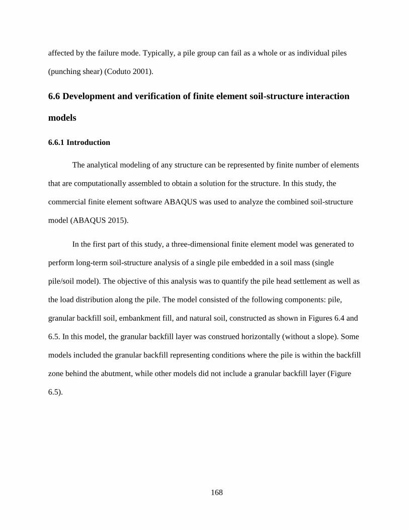
168
affected by the failure mode. Typically, a pile group can fail as a whole or as individual piles
(punching shear) (Coduto 2001).
6.6 Development and verification of finite element soil-structure interaction
models
6.6.1 Introduction
The analytical modeling of any structure can be represented by finite number of elements
that are computationally assembled to obtain a solution for the structure. In this study, the
commercial finite element software ABAQUS was used to analyze the combined soil-structure
model (ABAQUS 2015).
In the first part of this study, a three-dimensional finite element model was generated to
perform long-term soil-structure analysis of a single pile embedded in a soil mass (single
pile/soil model). The objective of this analysis was to quantify the pile head settlement as well as
the load distribution along the pile. The model consisted of the following components: pile,
granular backfill soil, embankment fill, and natural soil, constructed as shown in Figures 6.4 and
6.5. In this model, the granular backfill layer was construed horizontally (without a slope). Some
models included the granular backfill representing conditions where the pile is within the backfill
zone behind the abutment, while other models did not include a granular backfill layer (Figure
6.5).
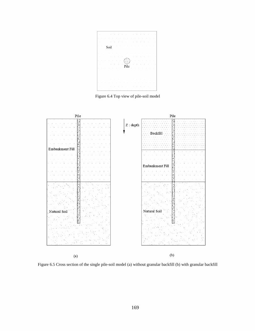
169
Figure 6.4 Top view of pile-soil model
Figure 6.5 Cross section of the single pile-soil model (a) without granular backfill (b) with granular backfill
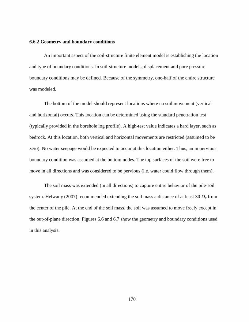
170
6.6.2 Geometry and boundary conditions
An important aspect of the soil-structure finite element model is establishing the location
and type of boundary conditions. In soil-structure models, displacement and pore pressure
boundary conditions may be defined. Because of the symmetry, one-half of the entire structure
was modeled.
The bottom of the model should represent locations where no soil movement (vertical
and horizontal) occurs. This location can be determined using the standard penetration test
(typically provided in the borehole log profile). A high-test value indicates a hard layer, such as
bedrock. At this location, both vertical and horizontal movements are restricted (assumed to be
zero). No water seepage would be expected to occur at this location either. Thus, an impervious
boundary condition was assumed at the bottom nodes. The top surfaces of the soil were free to
move in all directions and was considered to be pervious (i.e. water could flow through them).
The soil mass was extended (in all directions) to capture entire behavior of the pile-soil
system. Helwany (2007) recommended extending the soil mass a distance of at least 30 Dp from
the center of the pile. At the end of the soil mass, the soil was assumed to move freely except in
the out-of-plane direction. Figures 6.6 and 6.7 show the geometry and boundary conditions used
in this analysis.

171
Figure 6.6 Boundary condition of the pile-soil model (top view)
Figure 6.7 Boundary condition of the single pile-soil model with or without the backfill layer (vertical section)
In the above figures,
Z = Depth reference.
Hb = Height of the backfill,

172
He = Height of the embankment fill.
Hn = Depth the natural soil (to impervious layer).
Lp = Length of pile.
Wsoil = Width of the modeled soil medium.
Lsoil = Length of the modeled soil medium.
A parametric study was conducted in the single pile-soil model. Values of Hb, He, Hn, Lp,
and Dp were varied according to the parametric study matrix shown in Table 6.2 (see Section
6.7).
6.6.3 Contact behavior at structure-soil interfaces
The developed three-dimensional model include interaction between the pile and the
surrounding soil. Interface elements were introduced across these interfaces to transfer normal
and tangential forces using the pressure-overclosure relationship and coulomb friction model that
is defined within ABAQUS (see Section 4.2). In this analysis, the concrete surfaces (i.e. pile
shaft including the tip) were assigned to act as master elements while soil surfaces were assigned
to act as slave elements.
6.6.4 Analysis procedures for single pile-soil model
The analysis procedures used to run the single pile-soil model included the following
steps:
1- Applying a geostatic load on the underlying natural soil layer. In this step, the
effective self-weight of the natural soil was applied. The geostatic step assures

173
that equilibrium is satisfied within the natural soil layer, and that the initial stress
conditions in all elements falls within the initial yield surface.
2- Constructing the embankment fill over a period of time (equation 5-1). In this
step, the effective self-weight of the embankment soil was applied. This was done
in a coupled (consolidation) step where the load of the embankment is applied in a
timely manner.
3- Adding the pile and associated loads. This step was also done in a coupled
(consolidation) way where the soil is removed, and pile is added with a perfect
contact with the soil. The construction of the pile was assumed to occur ninety
days after the completion of the embankment fill and over a ten-day period.
4- Consolidation steps. In these steps, calculations to determine the primary
settlement (consolidation process) and secondary settlement (creep) were
performed.
6.6.5 Material properties
The concrete in the pile was assumed to behave in a linearly elastic manner with a
modulus of elasticity that was consistent with a design compressive strength of 4000 psi. Table
4.2 shows the concrete material parameters used. On the other hand, the modified Drucker-
Prager/Cap material model was used to simulate the behavior of the soils. Table 4.7 shows the
input parameters used to model the soil.
6.6.6 Initial model
An initial model was used in this phase of the study to determine the proper element size
and to conduct comparison analysis. The layout used in the initial model was similar to that
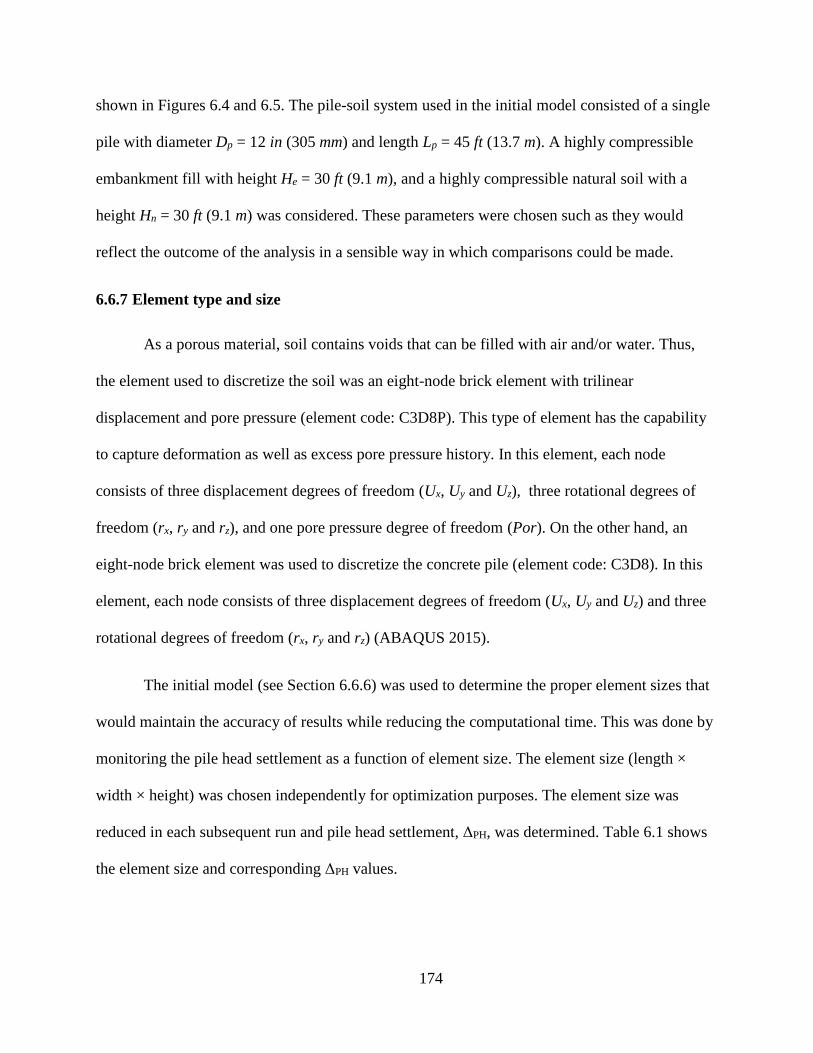
174
shown in Figures 6.4 and 6.5. The pile-soil system used in the initial model consisted of a single
pile with diameter Dp = 12 in (305 mm) and length Lp = 45 ft (13.7 m). A highly compressible
embankment fill with height He = 30 ft (9.1 m), and a highly compressible natural soil with a
height Hn = 30 ft (9.1 m) was considered. These parameters were chosen such as they would
reflect the outcome of the analysis in a sensible way in which comparisons could be made.
6.6.7 Element type and size
As a porous material, soil contains voids that can be filled with air and/or water. Thus,
the element used to discretize the soil was an eight-node brick element with trilinear
displacement and pore pressure (element code: C3D8P). This type of element has the capability
to capture deformation as well as excess pore pressure history. In this element, each node
consists of three displacement degrees of freedom (Ux, Uy and Uz), three rotational degrees of
freedom (rx, ry and rz), and one pore pressure degree of freedom (Por). On the other hand, an
eight-node brick element was used to discretize the concrete pile (element code: C3D8). In this
element, each node consists of three displacement degrees of freedom (Ux, Uy and Uz) and three
rotational degrees of freedom (rx, ry and rz) (ABAQUS 2015).
The initial model (see Section 6.6.6) was used to determine the proper element sizes that
would maintain the accuracy of results while reducing the computational time. This was done by
monitoring the pile head settlement as a function of element size. The element size (length ×
width × height) was chosen independently for optimization purposes. The element size was
reduced in each subsequent run and pile head settlement, ΔPH, was determined. Table 6.1 shows
the element size and corresponding ΔPH values.

175
Table 6.1 Element size versus simulated ΔPH
Element size Total
number of
elements
ΔPH in (mm)
Difference (from previous size)
(%)
Difference (from coarsest size)
(%) (height)
ft (m) (length × width)
ft (m)
5.0 (1.5) [1] 5.0 × 5.0 (1.5 × 1.5) [1] 4,176 3.47 (88) - -
2.0 (0.6) 5.0 × 5.0 (1.5 × 1.5) 10,788 3.66 (93) 5.5 5.0
1.0 (0.3) 5.0 × 5.0 (1.5 × 1.5) 20,880 3.71 (94) 1.3 6.0
0.5 (0.2) 5.0 × 5.0 (1.5 × 1.5) 41,760 3.72 (94) 0.2 7.0
2.0 (0.6) 2.0 × 2.0 (0.6 × 0.6) 29,760 3.67 (93) - 5.0
1.0 (0.3) 2.0 × 2.0 (0.6 × 0.6) 57,600 3.71 (94) 1.0 6.5
0.5 (0.2) 2.0 × 2.0 (0.6 × 0.6) 115,200 3.73 (95) 0.5 7.0
1.0 (0.3) 1.0 × 1.0 (0.3 × 0.3) 157,800 3.71 (94) - 6.5
0.5 (0.2) 1.0 × 1.0 (0.3 × 0.3) 315,600 3.73 (94) 0.5 7.0
0.5 (0.2) 0.5 × 0.5 (0.2 × 0.2) 1,022,200 3.77 (95) - 7.5 [1] coarsest element size
The results show that pile head settlement, ΔPH, becomes nearly steady (maximum error
of 0.5%) when the element size is at or less than 1.0 ft × 2.0 ft × 2.0 ft (0.30 m × 0.60 m × 0.60
m). Therefore, this element size was used in this study.
6.6.8 Comparison with analytical solution
In this part of the study, a finite element model was generated to simulate the long-term
load capacity of the pile-soil system. The simulated pile-soil capacity was then compared with
the analytical β-method. For this analysis, the soil-pile properties and conditions were identical
to those used in the initial model (see Section 6.6.6).
The simulated pile load-settlement analysis was carried out such that the pile’s head was
vertically displaced a total distance of about (0.25 Dp), and the force required to achieve the
displacement was recorded incrementally. The pile was displaced at this magnitude to assure the
mobilization of the pile tip bearing resistance (see Section 6.4.2). The vertical displacement was
imposed in a very slow rate of 1×10-15 in/sec (1×10-14 mm/sec). This was to prevent any excess
pore pressure from building up around the sides and tip of the pile. Figure 6.8 shows the
deformed contour of the modeled pile-soil system. Figure 6.9 shows the distribution of pore
pressure at the end of the analysis.

176
Figure 6.8 Vertical deformation contour at the end of the analysis (ft)
Figure 6.9 Excess pore pressure contour at the end of the analysis (psf)
The simulated load-settlement curve is shown in Figure 6.10. The figure shows that the
FEM load carrying capacity of the pile-soil system was 85 kips (380 kN) which compared to 92
kips (410 kN) using the β-method with a reasonably good agreement.
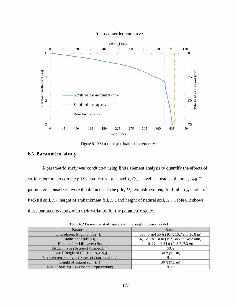
177
Figure 6.10 Simulated pile load-settlement curve
6.7 Parametric study
A parametric study was conducted using finite element analysis to quantify the effects of
various parameters on the pile’s load carrying capacity, Qu, as well as head settlement, ΔPH. The
parameters considered were the diameter of the pile, Dp, embedment length of pile, Lp, height of
backfill soil, Hb, height of embankment fill, He, and height of natural soil, Hn. Table 6.2 shows
these parameters along with their variation for the parametric study.
Table 6.2 Parametric study matrix for the single pile-soil model
Parameter Range
Embedment length of pile (Lp) 35, 45 and 55 ft (10.7, 13.7 and 16.8 m)
Diameter of pile (Dp) 6, 12, and 18 in (152, 305 and 458 mm)
Height of backfill layer (Hb) 0, 12 and 24 ft (0, 3.7, 7.3 m)
Backfill type (Degree of Compaction) 90%
Overall height of fill (Hf = He+ Hb) 30 ft (9.1 m)
Embankment soil type (Degree of Compressibility) High
Height of natural soil (Hn) 30 ft (9.1 m)
Natural soil type (Degree of Compressibility) High
0 45 90 135 180 225 270 315 360 405 450
0
25
50
75
0
1
2
3
0 10 20 30 40 50 60 70 80 90 100
Load (kN)
Pil
e hea
d s
ettl
emen
t (m
m)
Pil
e hea
d s
ettl
emen
t (i
n)
Load (kips)
Pile load-settlement curve
Simulated load-settlement curve
Simulated pile capacity
B-method capacity

178
Each pile size was examined using various choices of parameters to quantify their effect
on the pile head settlement. The pile head load, Q, was determined assuming that a line of piles
was placed between two 20-ft (6.1-m) approach slab segments with a thickness of 12 in (305
mm) and different transverse pile spacings. Table 6.3 shows the variation of all parameters tested
with each value of Dp.

179
Table 6.3 Range of parameters tested in accordance with Dp
Analysis No. Pile spacing[1]
ft (m)
Pile embedment length
Backfill
Lb ft (m)
Embankment fill
Le ft (m)
Natural soil
Ln ft (m)
Total embedment length
(Lp= Lb + Le + Ln) ft (m)
1 3 (0.9)
0 30 (9.1)
5 (1.5) 35 (10.7)
2 6 (1.8)
3 12 (3.7)
4 17 (5.2)
5 3 (0.9)
12 (3.7) 18 (5.5) 6 6 (1.8)
7 12 (3.7)
8 17 (5.2)
9 3 (0.9)
24 (7.3) 6 (1.8) 10 6 (1.8)
11 12 (3.7)
12 17 (5.2)
13 3 (0.9)
0 30 (9.1)
15 (4.6) 45 (13.7)
14 6 (1.8)
15 12 (3.7)
16 17 (5.2)
17 3 (0.9)
12 (3.7) 18 (5.5) 18 6 (1.8)
19 12 (3.7)
20 17 (5.2)
21 3 (0.9)
24 (7.3) 6 (1.8) 22 6 (1.8)
23 12 (3.7)
24 17 (5.2)
25 3 (0.9)
0 30 (9.1)
25 (7.6) 55 (16.8)
26 6 (1.8)
27 12 (3.7)
28 17 (5.2)
29 3 (0.9)
12 (3.7) 18 (5.5) 30 6 (1.8)
31 12 (3.7)
32 17 (5.2)
33 3 (0.9)
24 (7.3) 6 (1.8) 34 6 (1.8)
35 12 (3.7)
36 17 (5.2) [1] Piles were assumed to be on a line between two adjacent approach slab segments.
[1] For Dp = 12 in (305 mm), only pile spacing of 3, 6 and 12 ft (0.9, 1.8 and 3.7 m) were tested as pile capacity was reached. For
Dp = 6 in (152 mm), only pile spacing of 3 and 6 ft (0.9 and 1.8 m) were tested as pile capacity was reached (section 6.7.1).
The finite element model was generated as described in section 6.6. The models were run
for a simulated total time that allowed the completion of initial, primary (dissipation of water),
and secondary (creep) settlements of the modeled soil. The load on the embankment/backfill
layers was applied according to equation 5-1. The pile was installed ninety days after the

180
completion of the embankment/backfill after which the pile head load, Q, was applied in
accordance with Table 6.3. A typical finite element discretization of the single pile-soil model is
shown in Figures 6.11 and 6.12.
Figure 6.11 Finite element discretization of the single pile-soil model (No backfill)
Figure 6.12 Finite element discretization of the single pile-soil model (with backfill)

181
6.7.1 Load capacity of the pile
At this phase of the study, the load carrying capacity of the single pile-soil system as well
as the strength of pile material were evaluated. The ultimate carrying capacity of the pile-soil
system was evaluated using the β-method (see Section 6.4). This was compared with the
allowable load carrying capacity of the pile material using equation 6-4. Ultimately, the
controlling load (lowest) was selected to be the load carrying capacity of the pile. Table 6.4
shows result of this phase of the study.
Table 6.4 Pile load carrying capacity
Soil condition Pile configuration Capacity
Hb
ft (m) He
ft (m) Hn
ft (m) Dp
in (mm) Lp
ft (m)
β-method kips (kN)
Strength kips (kN)
Qps Qb Qu
0 30 (9.1)
30 (9.1)
18 (458)
35 (10.5)
33 (147) 29 (126) 62(273)
336 (1495)
12 (3.7) 18 (5.5) 33 (147) 28 (126) 61 (273)
24 (7.3) 6 (1.8) 33 (147) 28 (126) 61 (273)
0 30 (9.1)
45 (13.7)
58 (256) 35 (154) 92 (410)
12 (3.7) 18 (5.5) 56.5 (251) 33.5 (149) 90 (401)
24 (7.3) 6 (1.8) 57 (252) 34 (150) 91 (402)
0 30 (9.1)
55 (16.8)
87 (387) 40 (178) 127 (565)
12 (3.7) 18 (5.5) 85.5 (381) 39.5 (176) 125 (555)
24 (7.3) 6 (1.8) 85 (380) 39 (173) 124 (553)
0 30 (9.1)
12 (305)
35 (10.5)
24 (103) 12 (56) 35 (159)
149 (663)
12 (3.7) 18 (5.5) 23 (100) 12 (56) 35 (156)
24 (7.3) 6 (1.8) 23 (100) 12 (56) 35 (156)
0 30 (9.1)
45 (13.7)
39 (168) 15 (67) 54 (235)
12 (3.7) 18 (5.5) 38 (168) 15 (67) 53 (235)
24 (7.3) 6 (1.8) 38 (168) 15 (67) 53 (235)
0 30 (9.1)
55 (16.8)
58 (253) 18 (77) 76 (330)
12 (3.7) 18 (5.5) 57 (253) 17 (77) 74 (330)
24 (7.3) 6 (1.8) 57 (253) 17 (77) 74 (330)
0 30 (9.1)
6 (152)
35 (10.5)
11 (49) 3 (14) 14 (63)
37 (165)
12 (3.7) 18 (5.5) 11 (49) 3 (14) 14 (63)
24 (7.3) 6 (1.8) 11 (49) 3 (14) 14 (63)
0 30 (9.1)
45 (13.7)
19 (85) 4 (19) 23 (104)
12 (3.7) 18 (5.5) 19 (85) 4 (19) 23 (104)
24 (7.3) 6 (1.8) 19 (85) 4 (19) 23 (104)
0 30 (9.1)
55 (16.8)
29 (127) 4 (19) 33 (146)
12 (3.7) 18 (5.5) 29 (127) 4 (19) 33 (146)
24 (7.3) 6 (1.8) 29 (127) 4 (19) 33 (146)

182
6.7.2 Pile head settlement
The settlement of the pile head was of particular interest in this phase of the study. The
objective was to quantify the pile head settlement as a function of different pile-soil parameters
(see Tables 6.2 and 6.3). The result of the finite element analyses is shown in Figures 6.13, 6.14,
and 6.15.
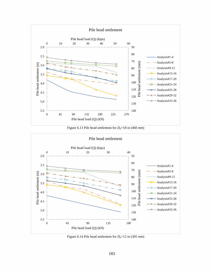
183
Figure 6.13 Pile head settlement for Dp=18 in (460 mm)
Figure 6.14 Pile head settlement for Dp=12 in (305 mm)
0 45 90 135 180 225 270
50
60
70
80
90
100
110
120
130
140
2.0
2.5
3.0
3.5
4.0
4.5
5.0
5.5
0 10 20 30 40 50 60
Pile head load (Q) (kN)
Pil
e hea
d s
ettl
emen
t (m
m)
Pil
e hea
d s
ettl
emen
t (i
n)
Pile head load (Q) (kips)
Pile head settlement
Analysis#1-4
Analysis#5-8
Analysis#9-12
Analysis#13-16
Analysis#17-20
Analysis#21-24
Analysis#25-28
Analysis#29-32
Analysis#33-36
0 45 90 135 180
50
60
70
80
90
100
110
120
130
140
2.0
2.5
3.0
3.5
4.0
4.5
5.0
5.5
0 10 20 30 40
Pile head load (Q) (kN)
Pil
e hea
d s
ettl
emen
t (m
m)
Pil
e hea
d s
ettl
emen
t (i
n)
Pile head load (Q) (kips)
Pile head settlement
Analysis#1-4
Analysis#5-8
Analysis#9-12
Analysis#13-16
Analysis#17-20
Analysis#21-24
Analysis#25-28
Analysis#29-32
Analysis#33-36
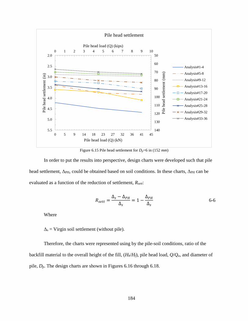
184
Figure 6.15 Pile head settlement for Dp=6 in (152 mm)
In order to put the results into perspective, design charts were developed such that pile
head settlement, ΔPH, could be obtained based on soil conditions. In these charts, ΔPH can be
evaluated as a function of the reduction of settlement, Rsett:
𝑅𝑠𝑒𝑡𝑡 =
∆𝑠 − ∆𝑃𝐻
∆𝑠= 1 −
∆𝑃𝐻
∆𝑠 6-6
Where
Δs = Virgin soil settlement (without pile).
Therefore, the charts were represented using by the pile-soil conditions, ratio of the
backfill material to the overall height of the fill, (Hb/Hf), pile head load, Q/Qu, and diameter of
pile, Dp. The design charts are shown in Figures 6.16 through 6.18.
0 5 9 14 18 23 27 32 36 41 45
50
60
70
80
90
100
110
120
130
140
2.0
2.5
3.0
3.5
4.0
4.5
5.0
5.5
0 1 2 3 4 5 6 7 8 9 10
Pile head load (Q) (kN)
Pil
e hea
d s
ettl
emen
t (m
m)
Pil
e hea
d s
ettl
emen
t (i
n)
Pile head load (Q) (kips)
Pile head settlement
Analysis#1-4
Analysis#5-8
Analysis#9-12
Analysis#13-16
Analysis#17-20
Analysis#21-24
Analysis#25-28
Analysis#29-32
Analysis#33-36
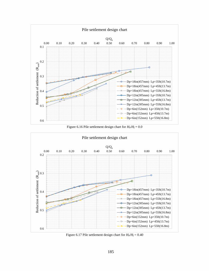
185
Figure 6.16 Pile settlement design chart for Hb/Hf = 0.0
Figure 6.17 Pile settlement design chart for Hb/Hf = 0.40
0.1
0.2
0.3
0.4
0.5
0.6
0.00 0.10 0.20 0.30 0.40 0.50 0.60 0.70 0.80 0.90 1.00
Red
uct
ion o
f se
ttle
men
t (
Rse
tt)
Q/Qu
Pile settlement design chart
Dp=18in(457mm) Lp=35ft(10.7m)
Dp=18in(457mm) Lp=45ft(13.7m)
Dp=18in(457mm) Lp=55ft(16.8m)
Dp=12in(305mm) Lp=35ft(10.7m)
Dp=12in(305mm) Lp=45ft(13.7m)
Dp=12in(305mm) Lp=55ft(16.8m)
Dp=6in(152mm) Lp=35ft(10.7m)
Dp=6in(152mm) Lp=45ft(13.7m)
Dp=6in(152mm) Lp=55ft(16.8m)

186
Figure 6.18 Pile settlement design chart for Hb/Hf = 0.80
The above design charts can be conveniently used to determine the most reliable design
option for a given pile-soil condition. Accordingly, the required size, length and number of piles
needed to achieve the desired level of settlement reduction, Rsett, or pile head settlement can be
readily estimated.
6.7.3 Load distribution along the pile shaft
This aspect of the study was focused on the load distribution along the pile. The objective
was to quantify the axial force distribution as a function of different pile-soil conditions (see
Tables 6.2 and 6.3). The simulated axial force distributions are shown in Figures 6.19 to 6.45
0.3
0.4
0.5
0.6
0.00 0.10 0.20 0.30 0.40 0.50 0.60 0.70 0.80 0.90 1.00
Red
uct
ion o
f se
ttle
men
t (
Rse
tt)
Q/Qu
Pile settlement design chart
Dp=18in(457mm) Lp=35ft(10.7m)
Dp=18in(457mm) Lp=45ft(13.7m)
Dp=18in(457mm) Lp=55ft(16.8m)
Dp=12in(305mm) Lp=35ft(10.7m)
Dp=12in(305mm) Lp=45ft(13.7m)
Dp=12in(305mm) Lp=55ft(16.8m)
Dp=6in(152mm) Lp=35ft(10.7m)
Dp=6in(152mm) Lp=45ft(13.7m)
Dp=6in(152mm) Lp=55ft(16.8m)

187
Figure 6.19 Axial force distribution in pile with Dp=18 in (460 mm), Lp=35 ft (10.7 m), and Hb/Hf=0
Figure 6.20 Axial force distribution in pile with Dp=18 in (460 mm), Lp=45 ft (13.7 m), and Hb/Hf=0
04590135180225270
0
1.5
3
4.5
6
7.5
9
10.5
12
0
5
10
15
20
25
30
35
40
0102030405060
Axial force (kN)
Z (
m)
Z (
ft)
Axial force (kips)
Axial force distribution in pile
Q=0
Q=13.5 kips (60 kN)
Q=18 kips (80 kN)
Q=36 kips (160 kN)
Q=51 kips (227 kN)
04590135180225270315
0
1.5
3
4.5
6
7.5
9
10.5
12
13.5
15
0
5
10
15
20
25
30
35
40
45
50
010203040506070
Axial force (kN)
Z (
m)
Z (
ft)
Axial force (kips)
Axial force distribution in pile
Q=0
Q=13.5 kips (60 kN)
Q=18 kips (80 kN)
Q=36 kips (160 kN)
Q=51 kips (227 kN)

188
Figure 6.21 Axial force distribution in pile with Dp=18 in (460 mm), Lp=55 ft (16.8 m), and Hb/Hf=0
Figure 6.22 Axial force distribution in pile with Dp=18 in (460 mm), Lp=35 ft (10.7 m), and Hb/Hf=0.40
04590135180225270315360
0
1.5
3
4.5
6
7.5
9
10.5
12
13.5
15
16.5
18
0
10
20
30
40
50
60
01020304050607080
Axial force (kN)
Z (
m)
Z (
ft)
Axial force (kips)
Axial force distribution in pile
Q=0
Q=13.5 kips (60 kN)
Q=18 kips (80 kN)
Q=36 kips (160 kN)
Q=51 kips (227 kN)
04590135180225270
0
1.5
3
4.5
6
7.5
9
10.5
12
0
5
10
15
20
25
30
35
40
0102030405060
Axial force (kN)
Z (
m)
Z (
ft)
Axial force (kips)
Axial force distribution in pile
Q=0
Q=13.5 kips (60 kN)
Q=18 kips (80 kN)
Q=36 kips (160 kN)
Q=51 kips (227 kN)
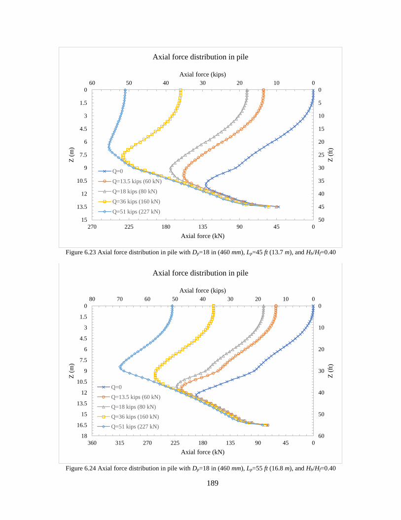
189
Figure 6.23 Axial force distribution in pile with Dp=18 in (460 mm), Lp=45 ft (13.7 m), and Hb/Hf=0.40
Figure 6.24 Axial force distribution in pile with Dp=18 in (460 mm), Lp=55 ft (16.8 m), and Hb/Hf=0.40
04590135180225270
0
1.5
3
4.5
6
7.5
9
10.5
12
13.5
15
0
5
10
15
20
25
30
35
40
45
50
0102030405060
Axial force (kN)
Z (
m)
Z (
ft)
Axial force (kips)
Axial force distribution in pile
Q=0
Q=13.5 kips (60 kN)
Q=18 kips (80 kN)
Q=36 kips (160 kN)
Q=51 kips (227 kN)
04590135180225270315360
0
1.5
3
4.5
6
7.5
9
10.5
12
13.5
15
16.5
18
0
10
20
30
40
50
60
01020304050607080
Axial force (kN)
Z (
m)
Z (
ft)
Axial force (kips)
Axial force distribution in pile
Q=0
Q=13.5 kips (60 kN)
Q=18 kips (80 kN)
Q=36 kips (160 kN)
Q=51 kips (227 kN)
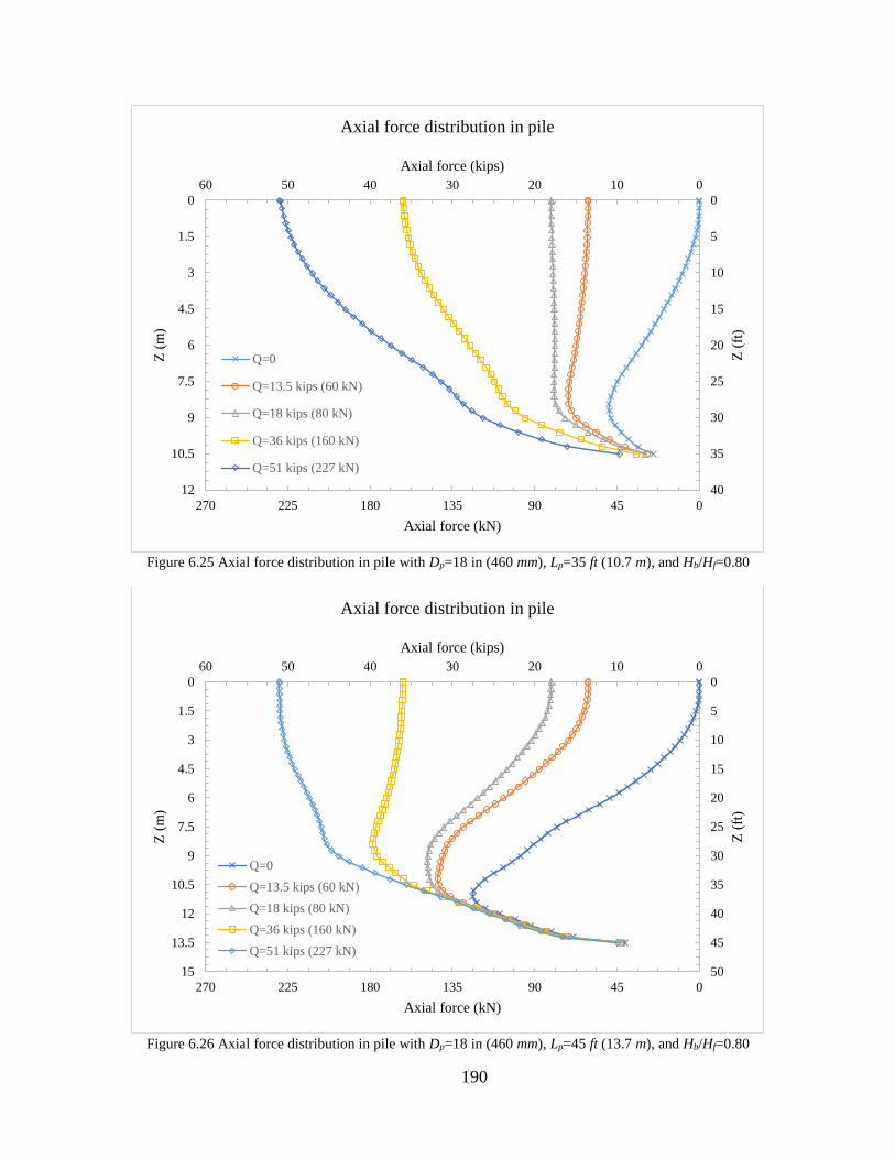
190
Figure 6.25 Axial force distribution in pile with Dp=18 in (460 mm), Lp=35 ft (10.7 m), and Hb/Hf=0.80
Figure 6.26 Axial force distribution in pile with Dp=18 in (460 mm), Lp=45 ft (13.7 m), and Hb/Hf=0.80
04590135180225270
0
1.5
3
4.5
6
7.5
9
10.5
12
0
5
10
15
20
25
30
35
40
0102030405060
Axial force (kN)
Z (
m)
Z (
ft)
Axial force (kips)
Axial force distribution in pile
Q=0
Q=13.5 kips (60 kN)
Q=18 kips (80 kN)
Q=36 kips (160 kN)
Q=51 kips (227 kN)
04590135180225270
0
1.5
3
4.5
6
7.5
9
10.5
12
13.5
15
0
5
10
15
20
25
30
35
40
45
50
0102030405060
Axial force (kN)
Z (
m)
Z (
ft)
Axial force (kips)
Axial force distribution in pile
Q=0
Q=13.5 kips (60 kN)
Q=18 kips (80 kN)
Q=36 kips (160 kN)
Q=51 kips (227 kN)
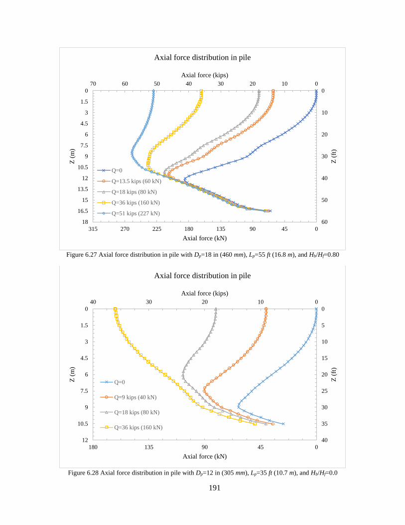
191
Figure 6.27 Axial force distribution in pile with Dp=18 in (460 mm), Lp=55 ft (16.8 m), and Hb/Hf=0.80
Figure 6.28 Axial force distribution in pile with Dp=12 in (305 mm), Lp=35 ft (10.7 m), and Hb/Hf=0.0
04590135180225270315
0
1.5
3
4.5
6
7.5
9
10.5
12
13.5
15
16.5
18
0
10
20
30
40
50
60
010203040506070
Axial force (kN)
Z (
m)
Z (
ft)
Axial force (kips)
Axial force distribution in pile
Q=0
Q=13.5 kips (60 kN)
Q=18 kips (80 kN)
Q=36 kips (160 kN)
Q=51 kips (227 kN)
04590135180
0
1.5
3
4.5
6
7.5
9
10.5
12
0
5
10
15
20
25
30
35
40
010203040
Axial force (kN)
Z (
m)
Z (
ft)
Axial force (kips)
Axial force distribution in pile
Q=0
Q=9 kips (40 kN)
Q=18 kips (80 kN)
Q=36 kips (160 kN)

192
Figure 6.29 Axial force distribution in pile with Dp=12 in (305 mm), Lp=45 ft (13.7 m), and Hb/Hf=0.0
Figure 6.30 Axial force distribution in pile with Dp=12 in (305 mm), Lp=55 ft (16.8 m), and Hb/Hf=0.0
04590135180225
0
1.5
3
4.5
6
7.5
9
10.5
12
13.5
15
0
5
10
15
20
25
30
35
40
45
50
01020304050
Axial force (kN)
Z (
m)
Z (
ft)
Axial force (kips)
Axial force distribution in pile
Q=0
Q=9 kips (40 kN)
Q=18 kips (80 kN)
Q=36 kips (160 kN)
04590135180225
0
1.5
3
4.5
6
7.5
9
10.5
12
13.5
15
16.5
18
0
10
20
30
40
50
60
01020304050
Axial force (kN)
Z (
m)
Z (
ft)
Axial force (kips)
Axial force distribution in pile
Q=0
Q=9 kips (40 kN)
Q=18 kips (80 kN)
Q=36 kips (160 kN)
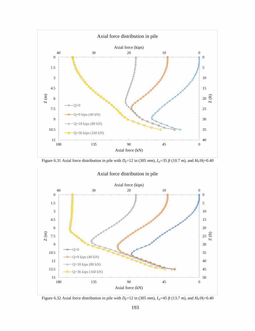
193
Figure 6.31 Axial force distribution in pile with Dp=12 in (305 mm), Lp=35 ft (10.7 m), and Hb/Hf=0.40
Figure 6.32 Axial force distribution in pile with Dp=12 in (305 mm), Lp=45 ft (13.7 m), and Hb/Hf=0.40
04590135180
0
1.5
3
4.5
6
7.5
9
10.5
12
0
5
10
15
20
25
30
35
40
010203040
Axial force (kN)
Z (
m)
Z (
ft)
Axial force (kips)
Axial force distribution in pile
Q=0
Q=9 kips (40 kN)
Q=18 kips (80 kN)
Q=36 kips (160 kN)
04590135180
0
1.5
3
4.5
6
7.5
9
10.5
12
13.5
15
0
5
10
15
20
25
30
35
40
45
50
010203040
Axial force (kN)
Z (
m)
Z (
ft)
Axial force (kips)
Axial force distribution in pile
Q=0
Q=9 kips (40 kN)
Q=18 kips (80 kN)
Q=36 kips (160 kN)

194
Figure 6.33 Axial force distribution in pile with Dp=12 in (305 mm), Lp=35 ft (16.8 m), and Hb/Hf=0.40
Figure 6.34 Axial force distribution in pile with Dp=12 in (305 mm), Lp=35 ft (10.7 m), and Hb/Hf=0.80
04590135180225
0
1.5
3
4.5
6
7.5
9
10.5
12
13.5
15
16.5
18
0
10
20
30
40
50
60
01020304050
Axial force (kN)
Z (
m)
Z (
ft)
Axial force (kips)
Axial force distribution in pile
Q=0
Q=9 kips (40 kN)
Q=18 kips (80 kN)
Q=36 kips (160 kN)
04590135180
0
1.5
3
4.5
6
7.5
9
10.5
12
0
5
10
15
20
25
30
35
40
010203040
Axial force (kN)
Z (
m)
Z (
ft)
Axial force (kips)
Axial force distribution in pile
Q=0
Q=9 kips (40 kN)
Q=18 kips (80 kN)
Q=36 kips (160 kN)

195
Figure 6.35 Axial force distribution in pile with Dp=12 in (305 mm), Lp=45 ft (13.7 m), and Hb/Hf=0.80
Figure 6.36 Axial force distribution in pile with Dp=12 in (305 mm), Lp=55 ft (16.8 m), and Hb/Hf=0.80
04590135180
0
1.5
3
4.5
6
7.5
9
10.5
12
13.5
15
0
5
10
15
20
25
30
35
40
45
50
010203040
Axial force (kN)
Z (
m)
Z (
ft)
Axial force (kips)
Axial force distribution in pile
Q=0
Q=9 kips (40 kN)
Q=18 kips (80 kN)
Q=36 kips (160 kN)
04590135180225
0
1.5
3
4.5
6
7.5
9
10.5
12
13.5
15
16.5
18
0
10
20
30
40
50
60
01020304050
Axial force (kN)
Z (
m)
Z (
ft)
Axial force (kips)
Axial force distribution in pile
Q=0
Q=9 kips (40 kN)
Q=18 kips (80 kN)
Q=36 kips (160 kN)

196
Figure 6.37 Axial force distribution in pile with Dp=6 in (152 mm), Lp=35 ft (10.7 m), and Hb/Hf=0.0
Figure 6.38 Axial force distribution in pile with Dp=6 in (152 mm), Lp=45 ft (13.7 m), and Hb/Hf=0.0
04590
0
1.5
3
4.5
6
7.5
9
10.5
12
0
5
10
15
20
25
30
35
40
01020
Axial force (kN)
Z (
m)
Z (
ft)
Axial force (kips)
Axial force distribution in pile
Q=0
Q=4.5 kips (20 kN)
Q=9 kips (40 kN)
04590
0
1.5
3
4.5
6
7.5
9
10.5
12
13.5
15
0
5
10
15
20
25
30
35
40
45
50
01020
Axial force (kN)
Z (
m)
Z (
ft)
Axial force (kips)
Axial force distribution in pile
Q=0
Q=4.5 kips (20 kN)
Q=9 kips (40 kN)

197
Figure 6.39 Axial force distribution in pile with Dp=6 in (152 mm), Lp=55 ft (16.8 m), and Hb/Hf=0.0
Figure 6.40 Axial force distribution in pile with Dp=6 in (152 mm), Lp=35 ft (10.7 m), and Hb/Hf=0.40
04590
0
1.5
3
4.5
6
7.5
9
10.5
12
13.5
15
16.5
18
0
10
20
30
40
50
60
01020
Axial force (kN)
Z (
m)
Z (
ft)
Axial force (kips)
Axial force distribution in pile
Q=0
Q=4.5 kips (20 kN)
Q=9 kips (40 kN)
04590
0
1.5
3
4.5
6
7.5
9
10.5
12
0
5
10
15
20
25
30
35
40
01020
Axial force (kN)
Z (
m)
Z (
ft)
Axial force (kips)
Axial force distribution in pile
Q=0
Q=4.5 kips (20 kN)
Q=9 kips (40 kN)

198
Figure 6.41 Axial force distribution in pile with Dp=6 in (152 mm), Lp=45 ft (13.7 m), and Hb/Hf=0.40
Figure 6.42 Axial force distribution in pile with Dp=6 in (152 mm), Lp=45 ft (13.7 m), and Hb/Hf=0.40
04590
0
1.5
3
4.5
6
7.5
9
10.5
12
13.5
15
0
5
10
15
20
25
30
35
40
45
50
01020
Axial force (kN)
Z (
m)
Z (
ft)
Axial force (kips)
Axial force distribution in pile
Q=0
Q=4.5 kips (20 kN)
Q=9 kips (40 kN)
04590
0
1.5
3
4.5
6
7.5
9
10.5
12
13.5
15
16.5
18
0
10
20
30
40
50
60
01020
Axial force (kN)
Z (
m)
Z (
ft)
Axial force (kips)
Axial force distribution in pile
Q=0
Q=4.5 kips (20 kN)
Q=9 kips (40 kN)

199
Figure 6.43 Axial force distribution in pile with Dp=6 in (152 mm), Lp=35 ft (10.7 m), and Hb/Hf=0.80
Figure 6.44 Axial force distribution in pile with Dp=6 in (152 mm), Lp=45 ft (13.7 m), and Hb/Hf=0.80
045
0
1.5
3
4.5
6
7.5
9
10.5
12
0
5
10
15
20
25
30
35
40
010
Axial force (kN)
Z (
m)
Z (
ft)
Axial force (kips)
Axial force distribution in pile
Q=0
Q=4.5 kips (20 kN)
Q=9 kips (40 kN)
04590
0
1.5
3
4.5
6
7.5
9
10.5
12
13.5
15
0
5
10
15
20
25
30
35
40
45
50
01020
Axial force (kN)
Z (
m)
Z (
ft)
Axial force (kips)
Axial force distribution in pile
Q=0
Q=4.5 kips (20 kN)
Q=9 kips (40 kN)

200
Figure 6.45 Axial force distribution in pile with Dp=6 in (152 mm), Lp=55 ft (16.8 m), and Hb/Hf=0.80
From the above figures, it is clear that the pile-soil systems resisted the applied load using
a combination of Qs and Qb. This indicates that the soil surrounding and underneath the pile
developed enough force that restrained the pile tip from sinking into the soil below it. As a result,
the pile was subjected to a downdrag force that was developed due to the consolidation of the
surrounding soils. The magnitude of the downdrag force varied depending on the properties of
the surrounding soil, pile geometry, and installation time. The neutral point, Ldd, appeared to be
dependent on the applied load, Q, and the length of pile, Lp. In the above figures, it was noted
that Ldd shifted upward as Q approached Qu and shifted downward as Lp increased. These are
illustrated in Figures 6.46 and 6.47.
04590
0
1.5
3
4.5
6
7.5
9
10.5
12
13.5
15
16.5
18
0
5
10
15
20
25
30
35
40
45
50
55
60
01020
Axial force (kN)
Z (
m)
Z (
ft)
Axial force (kips)
Axial force distribution in pile
Q=0
Q=4.5 kips (20 kN)
Q=9 kips (40 kN)
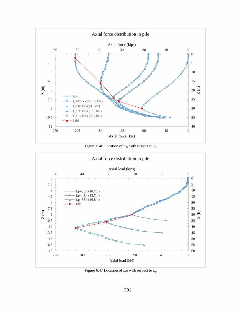
201
Figure 6.46 Location of Ldd with respect to Q
Figure 6.47 Location of Ldd with respect to Lp
04590135180225270
0
1.5
3
4.5
6
7.5
9
10.5
12
0
5
10
15
20
25
30
35
40
0102030405060
Axial force (kN)
Z (
m)
Z (
ft)
Axial force (kips)
Axial force distribution in pile
Q=0
Q=13.5 kips (60 kN)
Q=18 kips (80 kN)
Q=36 kips (160 kN)
Q=51 kips (227 kN)
Ldd
04590135180225
0
1.5
3
4.5
6
7.5
9
10.5
12
13.5
15
16.5
18
0
5
10
15
20
25
30
35
40
45
50
55
60
01020304050
Axial load (kN)
Z (
m)
Z (
ft)
Axial load (kips)
Axial force distribution in pile
Lp=35ft (10.7m)
Lp=45ft (13.7m)
Lp=55ft (16.8m)
Ldd

202
It was also noted that when backfill material is employed (i.e. Hb/Hf > 0), the location of
Ldd did not change compared to similar pile-soil condition with no backfill material (i.e. Hb/Hf =
0). However, the downdrag force, Qdd, decreased significantly as (Hb/Hf) increased, as illustrated
in Figure 6.48. This behavior can be attributed to the highly permeable backfill material. By the
time the pile is installed, the backfill material would have undergone initial and primary
settlement (consolidation), and thus lower forces were encountered in such cases.
Figure 6.48 Axial force distribution with respect to (Hb/Hf)
6.7.4 Proximity to the abutment wall
As discussed in Chapter 5, the abutment wall has a significant effect on the soil
deformation in its vicinity. The influence zone, in which soil deformation is affected by the
abutment, depends on the abutment wall to fill height ratio, and can affect the longitudinal soil
deformation to a distance of 10-60 ft (3-18 m) from the bridge abutment. However, a much
04590135180
0
1.5
3
4.5
6
7.5
9
10.5
12
13.5
15
0
5
10
15
20
25
30
35
40
45
50
010203040
Axial force (kN)
Z (
m)
Z (
ft)
Axial force (kips)
Axial force distribution in pile
Hb/Hf=0.0
Hb/Hf=0.40
Hb/Hf=0.80
Ldd

203
smaller pile influence zone was encountered with the simulated pile-soil systems. Figure 6.49
shows the influence pile zone for two pile sizes that embedded in the same soil profile. The
figure shows that the pile influence zone was in the range of 1-4 ft (0.3-1.2 m).
Figure 6.49 Vertical soil deformation contour with respect to pile-soil influence zone (a) Dp = 18 in (b) Dp = 6 in
This effect, however, could be significant in cases where piles are installed close to the
abutment wall. In such cases, detailed analyses must be performed to examine the effect. As for
the purposes of this study, it can be concluded that the effect of the pile on the surrounding soil is
limited and insignificant, as piles are planned to be installed at least 15 ft (4.6 m) away from the
bridge abutment.
6.8 Evaluating pile head settlement using analytical method
The objective of this phase of the study was to develop empirical relationship that can
predict the pile head settlement for a given pile-soil condition. Such an equation would be
beneficial in making reliable predictions of the long-term differential settlement of the pile-

204
supported segmented approach slab system. An empirical equation was derived based upon the
FEM results obtained in section 6.7.
A correlation study was carried out in which the correlation coefficient between pile head
settlement and various parameters were determined. The study examined the correlation between
ΔPH and pile geometry, loading conditions, and soil conditions. Table 6.5 shows the results of
this analysis.
Table 6.5 Pearson's correlation coefficient between ΔPH and various pile geometry, loading and soil parameters
Parameter ΔPH
ΔPs 0.815
Dp 0.056
Lp -0.414
Eavg -0.894
Gavg -0.879
Q 0.327
Qu -0.161
Q/Qu 0.483
Qdd -0.272
Ldd -0.449
Qps 0.148
Lps 0.076
Qb 0.106
Gavg-dd -0.789
Gavg-ps -0.638
In the above table,
ΔPs = Soil post construction settlement = ultimate settlement – settlement at the time of
pile installation.
Eavg = Average modulus of elasticity of soil along the pile length =
(𝐸1𝐻1 + 𝐸2𝐻2 + ⋯ + 𝐸𝑛𝐻𝑛) 𝐿𝑝⁄
Gavg = Average shear modulus of soil along the pile length =
(𝐺1𝐻1 + 𝐺2𝐻2 + ⋯ + 𝐺𝑛𝐻𝑛) 𝐿𝑝⁄

205
Gavg-dd = Average shear modulus of soil along the pile length within downdrag zone =
(𝐺1𝐻1 + 𝐺2𝐻2 + ⋯ + 𝐺𝑛𝐻𝑛) 𝐿𝑑𝑑⁄
Gavg-ps = Average shear modulus of soil along the pile length within positive skin friction
zone = (𝐺1𝐻1 + 𝐺2𝐻2 + ⋯ + 𝐺𝑛𝐻𝑛) 𝐿𝑝𝑠⁄
Table 6.5 shows that strong correlation exists between ΔPH and ΔPs, Eavg, Gavg, Gavg-dd and
Gavg-ps. This indicates that ΔPH could be evaluated using the shear deformation along the sides of
the pile and axial deformation underneath the tip of the pile. Accordingly, a multi-parameter
linear regression analysis was carried out in which ΔPH was expressed in terms of ΔPs, Eavg, Gavg,
Gavg-dd and Gavg-ps as follows:
∆𝑃𝐻= ∆𝑃𝑠 + 𝛼𝑄𝑑𝑑 𝐿𝑑𝑑−𝑖𝑛𝑓
𝐴𝑠𝐺𝑎𝑣𝑔−𝑑𝑑
+ 𝛽𝑄𝑝𝑠𝐿𝑝𝑠−𝑖𝑛𝑓
𝐴𝑠𝐺𝑎𝑣𝑔−𝑝𝑠
+ 𝜂𝑄𝑏𝐿𝑏−𝑖𝑛𝑓
𝐴𝑝𝐸𝑏
+ 𝐶 6-7
Where
Eb = Modulus of elasticity of soil underneath the pile tip.
As = Surface area of the pile.
Ldd-inf = The length of the influence zone of the downdrag.
Lps-inf = The length of the influence zone of the positive skin friction.
Lb-inf = The length of the influence zone underneath the pile tip.
𝛼, 𝛽, 𝜂, and C = Regression parameters.
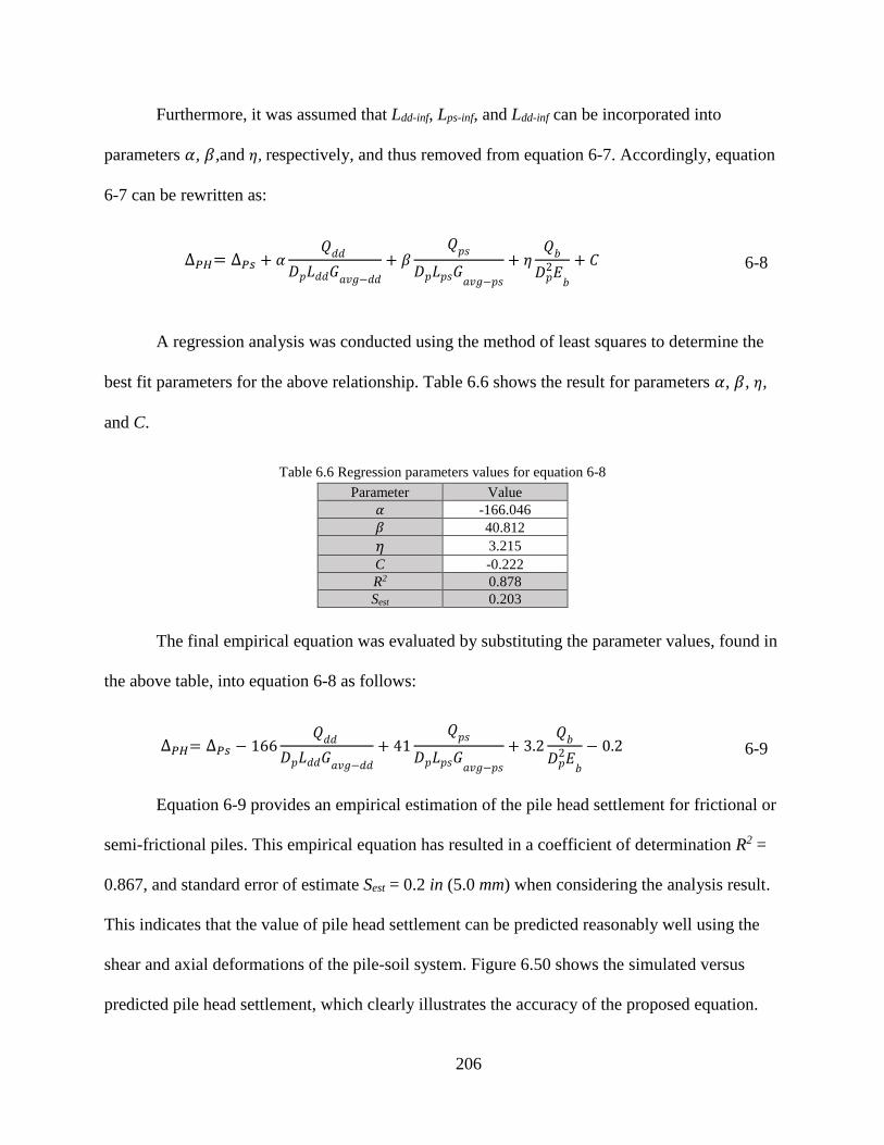
206
Furthermore, it was assumed that Ldd-inf, Lps-inf, and Ldd-inf can be incorporated into
parameters 𝛼, 𝛽,and 𝜂, respectively, and thus removed from equation 6-7. Accordingly, equation
6-7 can be rewritten as:
∆𝑃𝐻= ∆𝑃𝑠 + 𝛼𝑄𝑑𝑑
𝐷𝑝𝐿𝑑𝑑𝐺𝑎𝑣𝑔−𝑑𝑑
+ 𝛽𝑄𝑝𝑠
𝐷𝑝𝐿𝑝𝑠𝐺𝑎𝑣𝑔−𝑝𝑠
+ 𝜂𝑄𝑏
𝐷𝑝2𝐸
𝑏
+ 𝐶 6-8
A regression analysis was conducted using the method of least squares to determine the
best fit parameters for the above relationship. Table 6.6 shows the result for parameters 𝛼, 𝛽, 𝜂,
and C.
Table 6.6 Regression parameters values for equation 6-8
Parameter Value
𝛼 -166.046
𝛽 40.812
𝜂 3.215
C -0.222
R2 0.878
Sest 0.203
The final empirical equation was evaluated by substituting the parameter values, found in
the above table, into equation 6-8 as follows:
∆𝑃𝐻= ∆𝑃𝑠 − 166𝑄𝑑𝑑
𝐷𝑝𝐿𝑑𝑑𝐺𝑎𝑣𝑔−𝑑𝑑
+ 41𝑄𝑝𝑠
𝐷𝑝𝐿𝑝𝑠𝐺𝑎𝑣𝑔−𝑝𝑠
+ 3.2𝑄𝑏
𝐷𝑝2𝐸
𝑏
− 0.2 6-9
Equation 6-9 provides an empirical estimation of the pile head settlement for frictional or
semi-frictional piles. This empirical equation has resulted in a coefficient of determination R2 =
0.867, and standard error of estimate Sest = 0.2 in (5.0 mm) when considering the analysis result.
This indicates that the value of pile head settlement can be predicted reasonably well using the
shear and axial deformations of the pile-soil system. Figure 6.50 shows the simulated versus
predicted pile head settlement, which clearly illustrates the accuracy of the proposed equation.
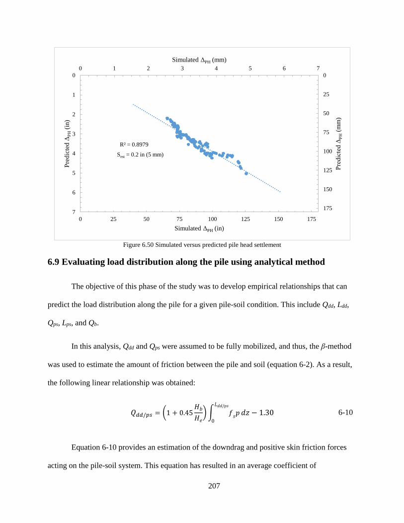
207
Figure 6.50 Simulated versus predicted pile head settlement
6.9 Evaluating load distribution along the pile using analytical method
The objective of this phase of the study was to develop empirical relationships that can
predict the load distribution along the pile for a given pile-soil condition. This include Qdd, Ldd,
Qps, Lps, and Qb.
In this analysis, Qdd and Qps were assumed to be fully mobilized, and thus, the β-method
was used to estimate the amount of friction between the pile and soil (equation 6-2). As a result,
the following linear relationship was obtained:
𝑄𝑑𝑑/𝑝𝑠 = (1 + 0.45
𝐻𝑏
𝐻𝑒
) ∫ 𝑓𝑠𝑝
𝐿𝑑𝑑/𝑝𝑠
0
𝑑𝑧 − 1.30 6-10
Equation 6-10 provides an estimation of the downdrag and positive skin friction forces
acting on the pile-soil system. This equation has resulted in an average coefficient of
Sest = 0.2 in (5 mm)
R² = 0.8979
0 25 50 75 100 125 150 175
0
25
50
75
100
125
150
175
0
1
2
3
4
5
6
7
0 1 2 3 4 5 6 7
Simulated ΔPH (in)
Pre
dic
ted
ΔP
H(m
m)
Pre
dic
ted
ΔP
H(i
n)
Simulated ΔPH (mm)
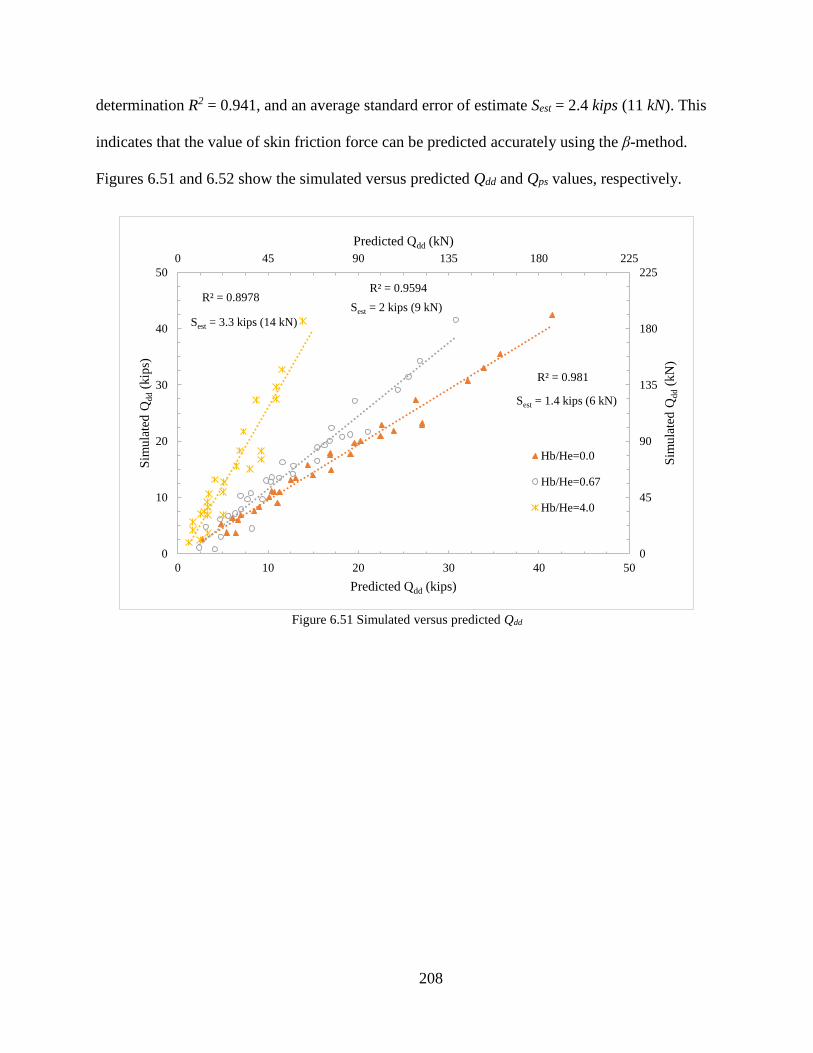
208
determination R2 = 0.941, and an average standard error of estimate Sest = 2.4 kips (11 kN). This
indicates that the value of skin friction force can be predicted accurately using the β-method.
Figures 6.51 and 6.52 show the simulated versus predicted Qdd and Qps values, respectively.
Figure 6.51 Simulated versus predicted Qdd
Sest = 1.4 kips (6 kN)
Sest = 2 kips (9 kN)
Sest = 3.3 kips (14 kN)
R² = 0.981
R² = 0.9594R² = 0.8978
0 45 90 135 180 225
0
45
90
135
180
225
0
10
20
30
40
50
0 10 20 30 40 50
Predicted Qdd (kN)
Sim
ula
ted
Qdd
(kN
)
Sim
ula
ted
Qdd
(kip
s)
Predicted Qdd (kips)
Hb/He=0.0
Hb/He=0.67
Hb/He=4.0

209
Figure 6.52 Simulated versus predicted (Qps)
Care must be taken as equation 6-10 can only be used when Ldd and Lps are known.
Bowles (1997) provides an equation to estimate Ldd when Q = 0 as follows:
𝐿𝑑𝑑 =
𝐿𝑝 − 𝐻𝑓
𝐿𝑑𝑑(
𝐿𝑝 − 𝐻𝑓
2+
𝛾𝑓′𝐻𝑓
𝛾𝑛′
) −2𝛾𝑓
′𝐻𝑓
𝛾𝑛′
6-11
Equation 6-11 appears to accurately predict the location of the neutral point for all
simulated piles with (Q = 0). Figure 6.53 shows the simulated versus predicted values for Ldd
using equation 6-11.
Sest = 1.4 kips (6 kN)
Sest = 2 kips (9 kN)Sest = 3.8 kips (17 kN)
R² = 0.981
R² = 0.9594R² = 0.8703
0 45 90 135 180 225
0
45
90
135
180
225
0
10
20
30
40
50
0 10 20 30 40 50
Predicted Qps (kN)
Sim
ula
ted
Qps
(kN
)
Sim
ula
ted
Qps
(kip
s)
Predicted Qps (kips)
Hb/He=0.0
Hb/He=0.67
Hb/He=4.0

210
Figure 6.53 Simulated versus predicted Ldd
However, Ldd changes as a function of Q (Figure 6.46). To evaluate this change, the
simulated pile load distribution, Figures 6.19 through 6.45, were reconstructed such that the
length of the pile, Lp, was normalized, i.e. Z/Lp. In addition, the axial load curves were idealized
into linear curves. This was to address the changes of Ldd in a linear fashion that would simply
the analysis, and thus convenient prediction can be made. Figures 6.54 through 6.80 show the
normalized/idealized pile load curves.
Sest = 0.7 ft (0.2 m)
R² = 0.9856
9 10.5 12 13.5 15
9
10.5
12
13.5
15
25
30
35
40
45
30 35 40 45
Predicted Ldd (m)
Sim
ula
ted
Ldd
(m)
Sim
ula
ted
Ldd
(ft)
Predicted Ldd (ft)

211
Figure 6.54 Normalized/Idealized pile load with Dp=18 in (460 mm), Lp=35 ft (10.7 m), and Hb/Hf=0
Figure 6.55 Normalized/Idealized pile load with Dp=18 in (460 mm), Lp=45 ft (13.7 m), and Hb/Hf=0
0
0.1
0.2
0.3
0.4
0.5
0.6
0.7
0.8
0.9
1
1.1
00.10.20.30.40.50.60.70.80.91
Z/L
p
Q/Qu
Axial force distribution in pile
Q/Qu=0
Q/Qu=0-idealized
Q/Qu=0.22
Q/Qu=0.22-idealized
Q/Qu=0.30
Q/Qu=0.30-idealized
Q/Qu=0.58
Q/Qu=0.58-idealized
Q/Qu=0.82
Q/Qu=0.82-idealized
Pile Capacity-idealized
0
0.1
0.2
0.3
0.4
0.5
0.6
0.7
0.8
0.9
1
1.1
00.10.20.30.40.50.60.70.80.91
Z/L
p
Q/Qu
Axial force distribution in pile
Q/Qu=0
Q/Qu=0-idealized
Q/Qu=0.15
Q/Qu=0.15-idealized
Q/Qu=0.20
Q/Qu=0.20-idealized
Q/Qu=0.39
Q/Qu=0.39-idealized
Q/Qu=0.55
Q/Qu=0.55-idealized
Pile Capacity-idealized

212
Figure 6.56 Normalized/Idealized pile load with Dp=18 in (460 mm), Lp=55 ft (16.8 m), and Hb/Hf=0
Figure 6.57 Normalized/Idealized pile load with Dp=18 in (460 mm), Lp=35 ft (10.7 m), and Hb/Hf=0.40
0
0.1
0.2
0.3
0.4
0.5
0.6
0.7
0.8
0.9
1
1.1
00.10.20.30.40.50.60.70.80.91
Z/L
p
Q/Qu
Axial force distribution in pile
Q/Qu=0
Q/Qu=0-idealized
Q/Qu=0.10
Q/Qu=0.10-idealized
Q/Qu=0.14
Q/Qu=0.14-idealized
Q/Qu=0.28
Q/Qu=0.28-idealized
Q/Qu=0.40
Q/Qu=0.40-idealized
Pile Capacity-idealized
0
0.1
0.2
0.3
0.4
0.5
0.6
0.7
0.8
0.9
1
1.1
00.10.20.30.40.50.60.70.80.91
Z/L
p
Q/Qu
Axial force distribution in pile
Q/Qu=0
Q/Qu=0-idealized
Q/Qu=0.22
Q/Qu=0.22-idealized
Q/Qu=0.30
Q/Qu=0.30-idealized
Q/Qu=0.59
Q/Qu=0.59-idealized
Q/Qu=0.84
Q/Qu=0.84-idealized
Pile Capacity-idealized

213
Figure 6.58 Normalized/Idealized pile load with Dp=18 in (460 mm), Lp=45 ft (13.7 m), and Hb/Hf=0.40
Figure 6.59 Normalized/Idealized pile load with Dp=18 in (460 mm), Lp=55 ft (16.8 m), and Hb/Hf=0.40
0
0.1
0.2
0.3
0.4
0.5
0.6
0.7
0.8
0.9
1
1.1
00.10.20.30.40.50.60.70.80.91
Z/L
p
Q/Qu
Axial force distribution in pile
Q/Qu=0
Q/Qu=0-idealized
Q/Qu=0.15
Q/Qu=0.15-idealized
Q/Qu=0.20
Q/Qu=0.20-idealized
Q/Qu=0.40
Q/Qu=0.40-idealized
Q/Qu=0.56
Q/Qu=0.56-idealized
Pile Capacity-idealized
0
0.1
0.2
0.3
0.4
0.5
0.6
0.7
0.8
0.9
1
1.1
00.10.20.30.40.50.60.70.80.91
Z/L
p
Q/Qu
Axial force distribution in pile
Q/Qu=0
Q/Qu=0-idealized
Q/Qu=0.11
Q/Qu=0.11-idealized
Q/Qu=0.14
Q/Qu=0.14-idealized
Q/Qu=0.29
Q/Qu=0.29-idealized
Q/Qu=0.40
Q/Qu=0.40-idealized
Pile Capacity-idealized

214
Figure 6.60 Normalized/Idealized pile load with Dp=18 in (460 mm), Lp=35 ft (10.7 m), and Hb/Hf=0.80
Figure 6.61 Normalized/Idealized pile load with Dp=18 in (460 mm), Lp=45 ft (13.7 m), and Hb/Hf=0.80
0
0.1
0.2
0.3
0.4
0.5
0.6
0.7
0.8
0.9
1
1.1
00.10.20.30.40.50.60.70.80.91
Z/L
p
Q/Qu
Axial force distribution in pile
Q/Qu=0
Q/Qu=0-idealized
Q/Qu=0.22
Q/Qu=0.22-idealized
Q/Qu=0.30
Q/Qu=0.30-idealized
Q/Qu=0.59
Q/Qu=0.59-idealized
Q/Qu=0.84
Q/Qu=0.84-idealized
Pile Capacity-idealized
0
0.1
0.2
0.3
0.4
0.5
0.6
0.7
0.8
0.9
1
1.1
00.10.20.30.40.50.60.70.80.91
Z/L
p
Q/Qu
Axial force distribution in pile
Q/Qu=0
Q/Qu=0-idealized
Q/Qu=0.15
Q/Qu=0.15-idealized
Q/Qu=0.20
Q/Qu=0.20-idealized
Q/Qu=0.40
Q/Qu=0.40-idealized
Q/Qu=0.56
Q/Qu=0.56-idealized
Pile Capacity-idealized

215
Figure 6.62 Normalized/Idealized pile load with Dp=18 in (460 mm), Lp=55 ft (16.8 m), and Hb/Hf=0.80
Figure 6.63 Normalized/Idealized pile load with Dp=12 in (305 mm), Lp=35 ft (10.7 m), and Hb/Hf=0.0
0
0.1
0.2
0.3
0.4
0.5
0.6
0.7
0.8
0.9
1
1.1
00.10.20.30.40.50.60.70.80.91
Z/L
p
Q/Qu
Axial force distribution in pile
Q/Qu=0
Q/Qu=0-idealized
Q/Qu=0.11
Q/Qu=0.11-idealized
Q/Qu=0.14
Q/Qu=0.14-idealized
Q/Qu=0.29
Q/Qu=0.29-idealized
Q/Qu=0.40
Q/Qu=0.40-idealized
Pile Capacity-idealized
0
0.1
0.2
0.3
0.4
0.5
0.6
0.7
0.8
0.9
1
1.1
00.10.20.30.40.50.60.70.80.91
Z/L
p
Q/Qu
Axial force distribution in pile
Q/Qu=0
Q/Qu=0-idealized
Q/Qu=0.26
Q/Qu=0.26-idealized
Q/Qu=0.52
Q/Qu=0.52-idealized
Pile Capacity-idealized
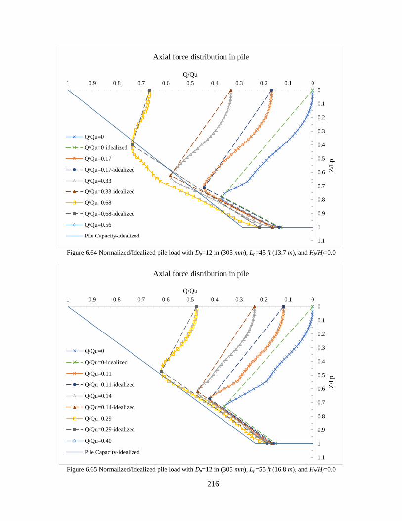
216
Figure 6.64 Normalized/Idealized pile load with Dp=12 in (305 mm), Lp=45 ft (13.7 m), and Hb/Hf=0.0
Figure 6.65 Normalized/Idealized pile load with Dp=12 in (305 mm), Lp=55 ft (16.8 m), and Hb/Hf=0.0
0
0.1
0.2
0.3
0.4
0.5
0.6
0.7
0.8
0.9
1
1.1
00.10.20.30.40.50.60.70.80.91
Z/L
p
Q/Qu
Axial force distribution in pile
Q/Qu=0
Q/Qu=0-idealized
Q/Qu=0.17
Q/Qu=0.17-idealized
Q/Qu=0.33
Q/Qu=0.33-idealized
Q/Qu=0.68
Q/Qu=0.68-idealized
Q/Qu=0.56
Pile Capacity-idealized
0
0.1
0.2
0.3
0.4
0.5
0.6
0.7
0.8
0.9
1
1.1
00.10.20.30.40.50.60.70.80.91
Z/L
p
Q/Qu
Axial force distribution in pile
Q/Qu=0
Q/Qu=0-idealized
Q/Qu=0.11
Q/Qu=0.11-idealized
Q/Qu=0.14
Q/Qu=0.14-idealized
Q/Qu=0.29
Q/Qu=0.29-idealized
Q/Qu=0.40
Pile Capacity-idealized
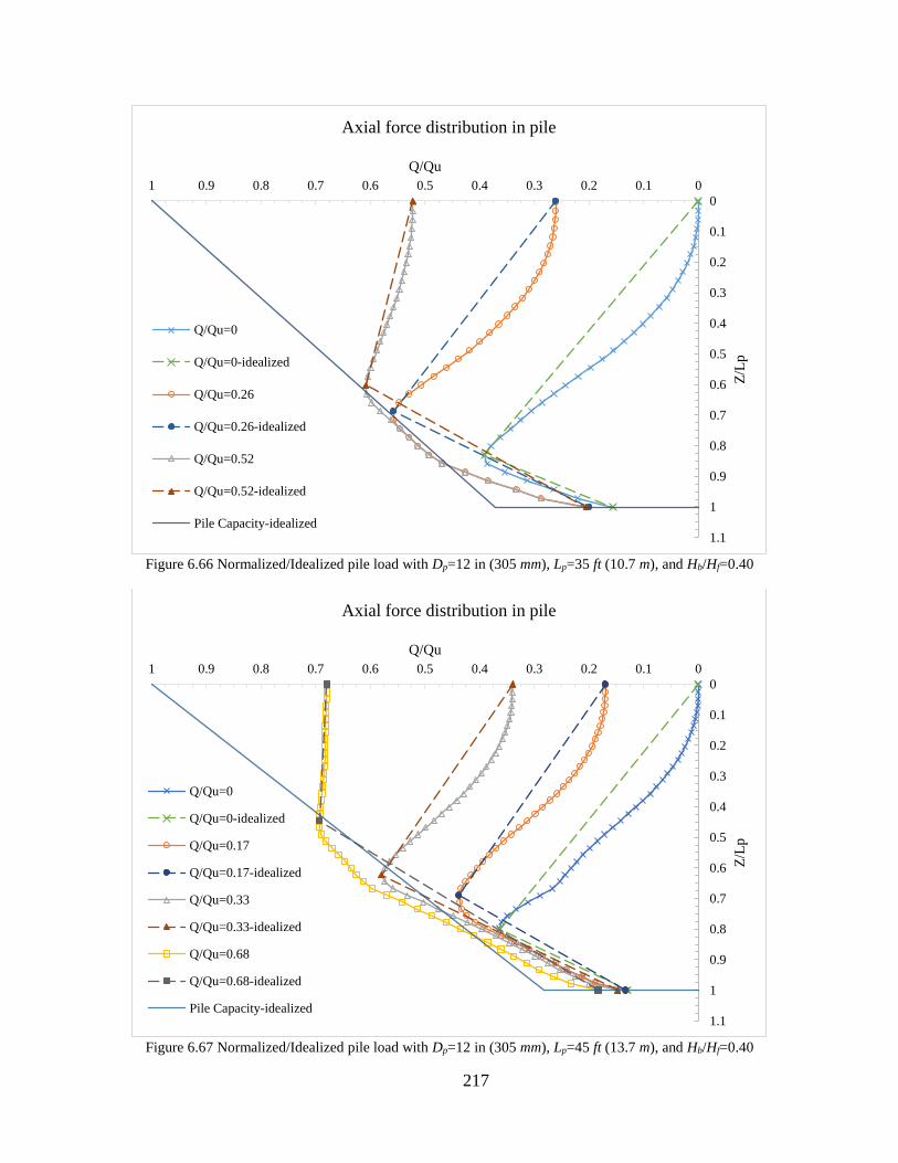
217
Figure 6.66 Normalized/Idealized pile load with Dp=12 in (305 mm), Lp=35 ft (10.7 m), and Hb/Hf=0.40
Figure 6.67 Normalized/Idealized pile load with Dp=12 in (305 mm), Lp=45 ft (13.7 m), and Hb/Hf=0.40
0
0.1
0.2
0.3
0.4
0.5
0.6
0.7
0.8
0.9
1
1.1
00.10.20.30.40.50.60.70.80.91
Z/L
p
Q/Qu
Axial force distribution in pile
Q/Qu=0
Q/Qu=0-idealized
Q/Qu=0.26
Q/Qu=0.26-idealized
Q/Qu=0.52
Q/Qu=0.52-idealized
Pile Capacity-idealized
0
0.1
0.2
0.3
0.4
0.5
0.6
0.7
0.8
0.9
1
1.1
00.10.20.30.40.50.60.70.80.91
Z/L
p
Q/Qu
Axial force distribution in pile
Q/Qu=0
Q/Qu=0-idealized
Q/Qu=0.17
Q/Qu=0.17-idealized
Q/Qu=0.33
Q/Qu=0.33-idealized
Q/Qu=0.68
Q/Qu=0.68-idealized
Pile Capacity-idealized

218
Figure 6.68 Normalized/Idealized pile load with Dp=12 in (305 mm), Lp=55 ft (16.8 m), and Hb/Hf=0.40
Figure 6.69 Normalized/Idealized pile load with Dp=12 in (305 mm), Lp=35 ft (10.7 m), and Hb/Hf=0.80
0
0.1
0.2
0.3
0.4
0.5
0.6
0.7
0.8
0.9
1
1.1
00.10.20.30.40.50.60.70.80.91
Z/L
p
Q/Qu
Axial force distribution in pile
Q/Qu=0
Q/Qu=0-idealized
Q/Qu=0.12
Q/Qu=0.12-idealized
Q/Qu=0.24
Q/Qu=0.24-idealized
Q/Qu=0.48
Q/Qu=0.48-idealized
Pile Capacity-idealized
0
0.1
0.2
0.3
0.4
0.5
0.6
0.7
0.8
0.9
1
1.1
00.10.20.30.40.50.60.70.80.91
Z/L
p
Q/Qu
Axial force distribution in pile
Q/Qu=0
Q/Qu=0-idealized
Q/Qu=0.26
Q/Qu=0.26-idealized
Q/Qu=0.52
Q/Qu=0.52-idealized
Pile Capacity-idealized

219
Figure 6.70 Normalized/Idealized pile load with Dp=12 in (305 mm), Lp=45 ft (13.7 m), and Hb/Hf=0.80
Figure 6.71 Normalized/Idealized pile load with Dp=12 in (305 mm), Lp=55 ft (16.8 m), and Hb/Hf=0.80
0
0.1
0.2
0.3
0.4
0.5
0.6
0.7
0.8
0.9
1
1.1
00.10.20.30.40.50.60.70.80.91
Z/L
p
Q/Qu
Axial force distribution in pile
Q/Qu=0
Q/Qu=0-idealized
Q/Qu=0.17
Q/Qu=0.17-idealized
Q/Qu=0.33
Q/Qu=0.33-idealized
Q/Qu=0.68
Q/Qu=0.68-idealized
Pile Capacity-idealized
0
0.1
0.2
0.3
0.4
0.5
0.6
0.7
0.8
0.9
1
1.1
00.10.20.30.40.50.60.70.80.91
Z/L
p
Q/Qu
Axial force distribution in pile
Q/Qu=0
Q/Qu=0-idealized
Q/Qu=0.11
Q/Qu=0.11-idealized
Q/Qu=0.14
Q/Qu=0.14-idealized
Q/Qu=0.29
Q/Qu=0.29-idealized
Pile Capacity-idealized

220
Figure 6.72 Normalized/Idealized pile load with Dp=6 in (152 mm), Lp=35 ft (10.7 m), and Hb/Hf=0.0
Figure 6.73 Normalized/Idealized pile load with Dp=6 in (152 mm), Lp=45 ft (13.7 m), and Hb/Hf=0.0
0
0.1
0.2
0.3
0.4
0.5
0.6
0.7
0.8
0.9
1
1.1
00.10.20.30.40.50.60.70.80.91
Z/L
p
Q/Qu
Axial force distribution in pile
Q/Qu=0
Q/Qu=0-idealized
Q/Qu=0.32
Q/Qu=0.32-idealized
Q/Qu=0.64
Q/Qu=0.64-idealized
Pile Capacity-idealized
0
0.1
0.2
0.3
0.4
0.5
0.6
0.7
0.8
0.9
1
1.1
00.10.20.30.40.50.60.70.80.91
Z/L
p
Q/Qu
Axial force distribution in pile
Q/Qu=0
Q/Qu=0-idealized
Q/Qu=0.20
Q/Qu=0.20-idealized
Q/Qu=0.39
Q/Qu=0.39-idealized
Pile Capacity-idealized
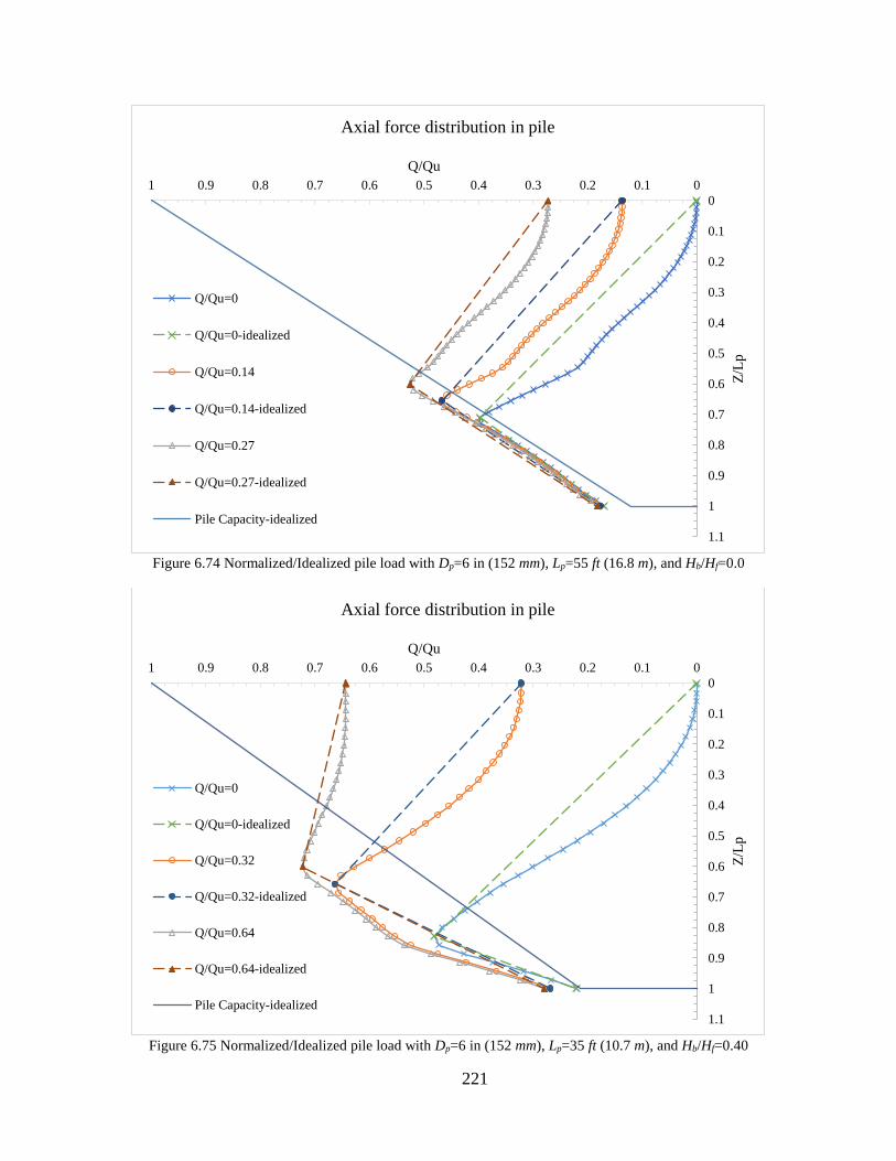
221
Figure 6.74 Normalized/Idealized pile load with Dp=6 in (152 mm), Lp=55 ft (16.8 m), and Hb/Hf=0.0
Figure 6.75 Normalized/Idealized pile load with Dp=6 in (152 mm), Lp=35 ft (10.7 m), and Hb/Hf=0.40
0
0.1
0.2
0.3
0.4
0.5
0.6
0.7
0.8
0.9
1
1.1
00.10.20.30.40.50.60.70.80.91
Z/L
p
Q/Qu
Axial force distribution in pile
Q/Qu=0
Q/Qu=0-idealized
Q/Qu=0.14
Q/Qu=0.14-idealized
Q/Qu=0.27
Q/Qu=0.27-idealized
Pile Capacity-idealized
0
0.1
0.2
0.3
0.4
0.5
0.6
0.7
0.8
0.9
1
1.1
00.10.20.30.40.50.60.70.80.91
Z/L
p
Q/Qu
Axial force distribution in pile
Q/Qu=0
Q/Qu=0-idealized
Q/Qu=0.32
Q/Qu=0.32-idealized
Q/Qu=0.64
Q/Qu=0.64-idealized
Pile Capacity-idealized
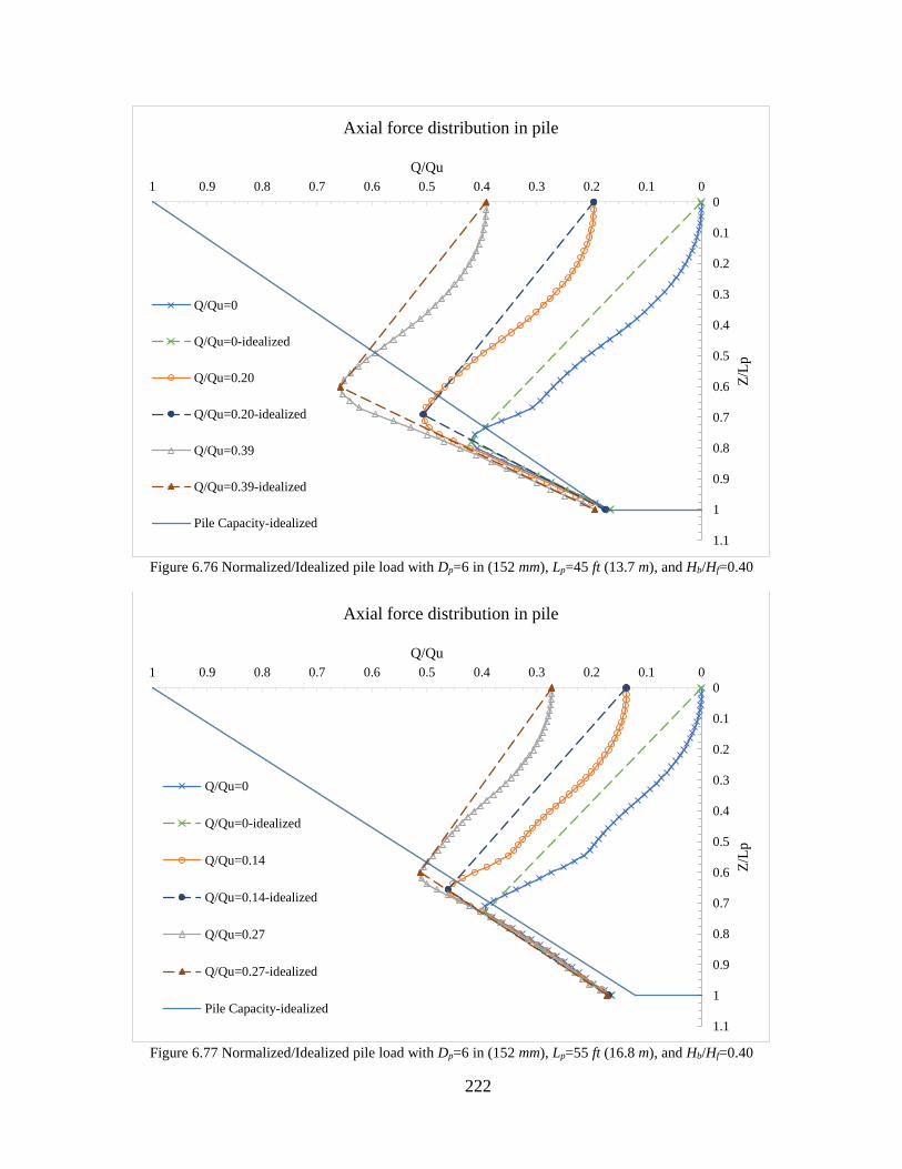
222
Figure 6.76 Normalized/Idealized pile load with Dp=6 in (152 mm), Lp=45 ft (13.7 m), and Hb/Hf=0.40
Figure 6.77 Normalized/Idealized pile load with Dp=6 in (152 mm), Lp=55 ft (16.8 m), and Hb/Hf=0.40
0
0.1
0.2
0.3
0.4
0.5
0.6
0.7
0.8
0.9
1
1.1
00.10.20.30.40.50.60.70.80.91
Z/L
p
Q/Qu
Axial force distribution in pile
Q/Qu=0
Q/Qu=0-idealized
Q/Qu=0.20
Q/Qu=0.20-idealized
Q/Qu=0.39
Q/Qu=0.39-idealized
Pile Capacity-idealized
0
0.1
0.2
0.3
0.4
0.5
0.6
0.7
0.8
0.9
1
1.1
00.10.20.30.40.50.60.70.80.91
Z/L
p
Q/Qu
Axial force distribution in pile
Q/Qu=0
Q/Qu=0-idealized
Q/Qu=0.14
Q/Qu=0.14-idealized
Q/Qu=0.27
Q/Qu=0.27-idealized
Pile Capacity-idealized

223
Figure 6.78 Normalized/Idealized pile load with Dp=6 in (152 mm), Lp=35 ft (10.7 m), and Hb/Hf=0.80
Figure 6.79 Normalized/Idealized pile load with Dp=6 in (152 mm), Lp=45 ft (13.7 m), and Hb/Hf=0.80
0
0.1
0.2
0.3
0.4
0.5
0.6
0.7
0.8
0.9
1
1.1
00.10.20.30.40.50.60.70.80.91
Z/L
p
Q/Qu
Axial force distribution in pile
Q/Qu=0
Q/Qu=0-idealized
Q/Qu=0.32
Q/Qu=0.32-idealized
Q/Qu=0.64
Q/Qu=0.64-idealized
Pile Capacity-idealized
0
0.1
0.2
0.3
0.4
0.5
0.6
0.7
0.8
0.9
1
1.1
00.10.20.30.40.50.60.70.80.91
Z/L
p
Q/Qu
Axial force distribution in pile
Q/Qu=0
Q/Qu=0-idealized
Q/Qu=0.20
Q/Qu=0.20-idealized
Q/Qu=0.39
Q/Qu=0.39-idealized
Pile Capacity-idealized
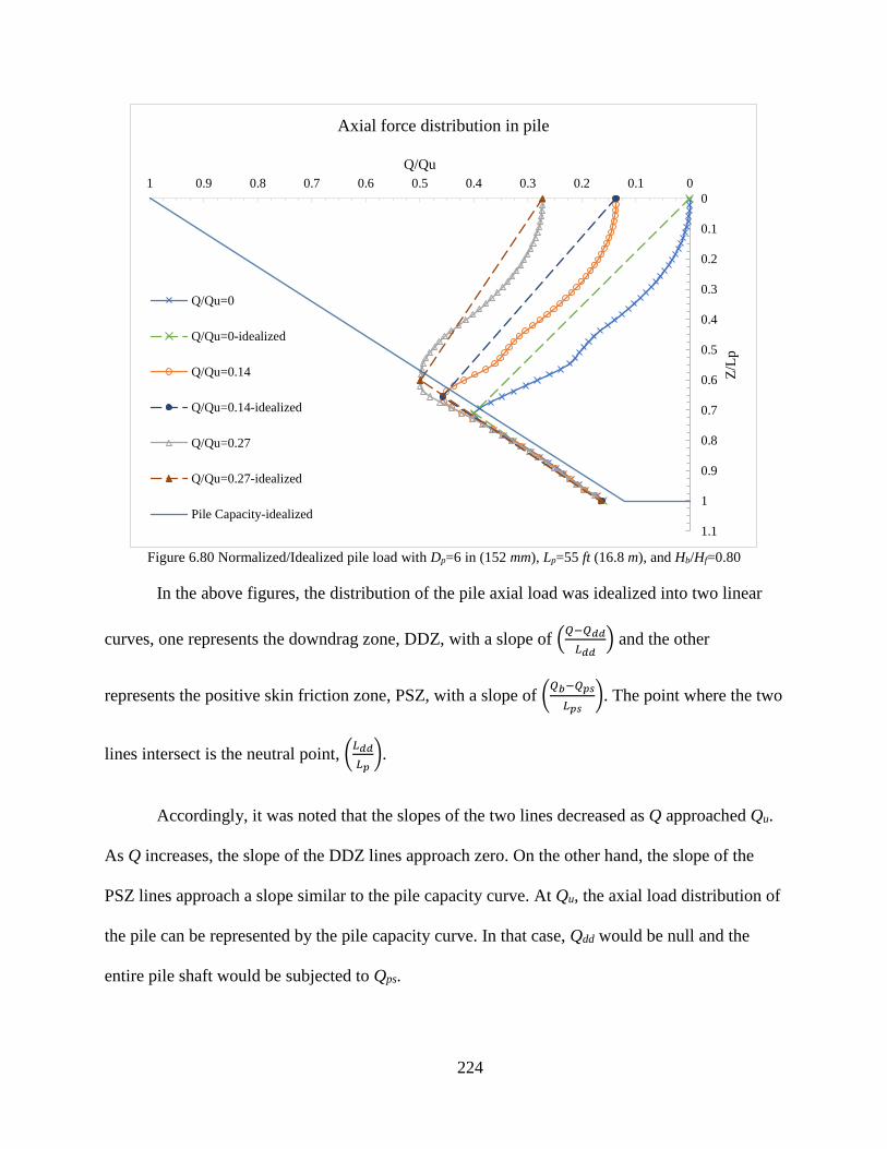
224
Figure 6.80 Normalized/Idealized pile load with Dp=6 in (152 mm), Lp=55 ft (16.8 m), and Hb/Hf=0.80
In the above figures, the distribution of the pile axial load was idealized into two linear
curves, one represents the downdrag zone, DDZ, with a slope of (𝑄−𝑄𝑑𝑑
𝐿𝑑𝑑) and the other
represents the positive skin friction zone, PSZ, with a slope of (𝑄𝑏−𝑄𝑝𝑠
𝐿𝑝𝑠). The point where the two
lines intersect is the neutral point, (𝐿𝑑𝑑
𝐿𝑝).
Accordingly, it was noted that the slopes of the two lines decreased as Q approached Qu.
As Q increases, the slope of the DDZ lines approach zero. On the other hand, the slope of the
PSZ lines approach a slope similar to the pile capacity curve. At Qu, the axial load distribution of
the pile can be represented by the pile capacity curve. In that case, Qdd would be null and the
entire pile shaft would be subjected to Qps.
0
0.1
0.2
0.3
0.4
0.5
0.6
0.7
0.8
0.9
1
1.1
00.10.20.30.40.50.60.70.80.91
Z/L
p
Q/Qu
Axial force distribution in pile
Q/Qu=0
Q/Qu=0-idealized
Q/Qu=0.14
Q/Qu=0.14-idealized
Q/Qu=0.27
Q/Qu=0.27-idealized
Pile Capacity-idealized

225
Additionally, it was noted that Qdd and Ldd were not only a function of Q, but also a
function of the consolidation level of the surrounding soil and the time of pile installation. This is
clearly shown in situations when (Hb/Hf >0) in which Ldd was never less than Hb. This indicates
that the pile was not subjected to Qdd within the backfill layer. The downdrag force in such cases
was a result of the consolidation (water dissipation) of the underneath embankment fill and
natural soil layers. When (Hb/Hf =0), the entire pile length could be subjected to downdrag force.
However, due to the installation time, part of the consolidation process could have undergone,
and thus low downdrag forces might be encountered in the top part of the pile (vicinity of the
surface of the soil). For the examined pile-soil parameters (see Tables 6.2 and 6.3), it was noted
that the piles were subjected to Qdd up to about (0.9-0.95 He). This indicates that, by the time of
installation, 5-10% of the embankment fill layer was undergone the consolidation process.
An attempt was made to establish relationships in which predict the axial load
distribution along the pile shaft. Assuming that the pile axial load distribution can be idealized
into two distinguish lines, i.e. DDZ and PSZ, linear relationships were sought in this phase of
the study (see Figure 6.81) using the normalized/idealized lines shown in Figures 6.54 through
6.80.

226
Figure 6.81 Development of axial load distribution in pile
In Figure 6.81, the DDZ lines can be establish utilizing the general form of a linear
relationship given as
𝑄
𝑄𝑢= 𝑚1 (
𝐿𝑑𝑑
𝐿𝑝) + 𝑐1 6-12
Where
m1 = Slope of the DDZ lines.
c1 = Constant.
227
The slope of the DDZ line decreases as Q/Qu approaches 1.0. In such case the slope of
the DDZ line would become 𝑚1@𝑄𝑢= 0. Using two slope points of 𝑚1@𝑄𝑢
= 0 and 𝑚1@𝑄=0=
(𝑄𝑑𝑑@𝑄=0 𝑄𝑢⁄ )
(𝐿𝑑𝑑@𝑄=0 𝐿𝑝⁄ ) with an assumed linear interpolation, m1 can be written as:
𝑚1 = (1 −
𝑄
𝑄𝑢) [
𝑄𝑑𝑑@𝑄=0𝐿𝑝
𝐿𝑑𝑑@𝑄=0𝑄𝑢
] 6-13
Where
𝑄𝑑𝑑@𝑄=0= Downdrag force when pile head load Q = 0 (equation 6-10)
𝐿𝑑𝑑@𝑄=0= Length of downdrag (neutral point) when pile head load Q = 0 (equation 6-11)
In equation 6-12, when Ldd/Lp = 0, c1 becomes
𝐶1 =
𝑄
𝑄𝑢 6-14
Substituting equations 6-13 and 6-14 into 6-12 yields Qdd at any pile head load, Q, as
follows:
𝑄𝑑𝑑
𝑄𝑢= (1 −
𝑄
𝑄𝑢) [
𝑄𝑑𝑑@𝑄=0𝐿𝑝
𝐿𝑑𝑑@𝑄=0𝑄𝑢
]𝐿𝑑𝑑
𝐿𝑝 6-15
Which reduces to
𝑄𝑑𝑑 = (𝑄𝑢 − 𝑄) [
𝑄𝑑𝑑@𝑄=0𝐿𝑑𝑑
𝐿𝑑𝑑@𝑄=0𝑄𝑢
] 6-16

228
The Qdd/Ldd line, shown in Figure 6.81, was introduced such that it passes through the
points (𝑄𝑑𝑑@𝑄=0
𝑄𝑢 ,
𝐿𝑑𝑑@𝑄=0
𝐿𝑝) and (
𝑄𝑢
𝑄𝑢 ,
𝐿𝑑𝑑@𝑄𝑑𝑑=0
𝐿𝑝).
Where
𝐿𝑑𝑑@𝑄𝑑𝑑=0
𝐿𝑝 = The embedded length of the pile at which not subjected to downdrag force
(consolidation line shown in Figure 6.81).
Thus, a linear relationship was established as follows:
𝑄
𝑄𝑢= 𝑚2 (
𝐿𝑑𝑑
𝐿𝑝) + 𝑐2 6-17
Where
m2 = Slope of the Qdd/Ldd line (see Figure 6.81).
c2 = Constant.
Since this line is passes through two fixed points, m2, can be written as follows:
𝑚2 =(𝑄𝑑𝑑@𝑄=0
𝑄𝑢⁄ ) − (𝑄𝑢 𝑄𝑢⁄ )
(𝐿𝑑𝑑@𝑄=0𝐿𝑝⁄ ) − (𝐿𝑑𝑑@𝑄𝑑𝑑=0
𝐿𝑝⁄ )=
(𝑄𝑑𝑑@𝑄=0− 𝑄𝑢)𝐿𝑝
(𝐿𝑑𝑑@𝑄=0− 𝐿𝑑𝑑@𝑄𝑑𝑑=0
) 𝑄𝑢
6-18
At (𝑄 𝑄𝑢⁄ ) = 1.0, (𝐿𝑑𝑑 𝐿𝑝⁄ ) = (𝐿𝑑𝑑@𝑄𝑑𝑑=0𝐿𝑝⁄ ). Therefore, c2, can be written as:
𝑐2 = 1 − 𝑚2 (𝐿𝑑𝑑@𝑄𝑑𝑑=0𝐿𝑝⁄ ) 6-19
Substituting equations 6-18 and 6-19 into 6-17 gives the Qdd/Ldd line as follows:

229
𝑄𝑑𝑑
𝑄𝑢=
(𝑄𝑑𝑑@𝑄=0− 𝑄𝑢) 𝐿𝑑𝑑
(𝐿𝑑𝑑@𝑄=0− 𝐿𝑑𝑑@𝑄𝑑𝑑=0
) 𝑄𝑢
+ [1 −(𝑄𝑑𝑑@𝑄=0
− 𝑄𝑢) 𝐿𝑑𝑑@𝑄𝑑𝑑=0
(𝐿𝑑𝑑@𝑄=0− 𝐿𝑑𝑑@𝑄𝑑𝑑=0
) 𝑄𝑢
] 6-20
Which can be reduced to
𝑄𝑑𝑑 = [(𝑄𝑑𝑑@𝑄=0
− 𝑄𝑢) 𝐿𝑑𝑑
(𝐿𝑑𝑑@𝑄=0− 𝐿𝑑𝑑@𝑄𝑑𝑑=0
)] + [𝑄𝑢 −
(𝑄𝑑𝑑@𝑄=0− 𝑄𝑢) 𝐿𝑑𝑑@𝑄𝑑𝑑=0
(𝐿𝑑𝑑@𝑄=0− 𝐿𝑑𝑑@𝑄𝑑𝑑=0
)] 6-21
Now, setting equation 6-16 equals to equation 6-21, Ldd can be expressed in terms of m1,
c1, m2 and c2 as follows:
𝐿𝑑𝑑 =𝑐2 − 𝑐1
𝑚1 − 𝑚2𝐿𝑝 6-22
Which can be expressed in terms of Q and L as follows:
𝐿𝑑𝑑 =
1 − [(𝑄𝑑𝑑@𝑄=0
− 𝑄𝑢) 𝐿𝑝
(𝐿𝑑𝑑@𝑄=0− 𝐿𝑑𝑑@𝑄𝑑𝑑=0
) 𝑄𝑢
(𝐿𝑑𝑑@𝑄𝑑𝑑=0
𝐿𝑝)] −
𝑄𝑄𝑢
(1 −𝑄
𝑄𝑢) [
𝑄𝑑𝑑@𝑄=0𝐿𝑝
𝐿𝑑𝑑@𝑄=0𝑄𝑢
] −(𝑄𝑑𝑑@𝑄=0
− 𝑄𝑢) 𝐿𝑝
(𝐿𝑑𝑑@𝑄=0− 𝐿𝑑𝑑@𝑄𝑑𝑑=0
) 𝑄𝑢
𝐿𝑝 6-23
Equations 6-16 and 6-23 provide an estimation of the downdrag force, Qdd, and neutral
point, Ldd, respectively. Figure 6.82 and Figure 6.83 show the simulated versus predicted Qdd and
Ldd using these equations, which illustrates the accuracy of the proposed equation.

230
Figure 6.82 Simulated versus predicted Qdd
Figure 6.83 Simulated versus predicted Ldd
Sest = 1.7 kips (8 kN)
R² = 0.9699
0 45 90 135 180 225
0
45
90
135
180
225
0
10
20
30
40
50
0 10 20 30 40 50
Predicted Qdd (kN)
Sim
ula
ted
Qdd
(kN
)
Sim
ula
ted
Qdd
(kip
s)
Predicted Qdd (kips)
Sest = 1.0 ft (0.3m)
R² = 0.9713
0 3 6 9 12 15
0
3
6
9
12
15
0
10
20
30
40
50
0 10 20 30 40 50
Predicted Ldd (m)
Sim
ula
ted
Ldd
(m)
Sim
ula
ted
Ldd
(ft)
Predicted Ldd (ft)

231
It should be noted that the establish of the latter relationships requires the pre-calculation
of 𝑄𝑑𝑑@𝑄=0 and 𝐿𝑑𝑑@𝑄=0
(blue lines shown in Figure 6.81) which can be evaluated using
equations 6-10 and 6-11, respectively. It should also be noted that a good engineering judgment
should be made regarding the location of the consolidation line, 𝐿𝑑𝑑@𝑄𝑑𝑑=0 (see Figure 6.81). A
value between 0.0-0.20 Lp appears to be a reasonable estimation for it. Table 6.7 shows different
values of assumed 𝐿𝑑𝑑@𝑄𝑑𝑑=0 versus predicted Ldd.
Table 6.7 Estimated 𝐿𝑑𝑑@𝑄𝑑𝑑=0 versus predicted Ldd
𝐿𝑑𝑑@𝑄𝑑𝑑=0
Ldd
R2 Sest
ft (m)
0.0 Lp 0.970 1.03 (0.31)
0.1 Lp 0.971 1.02 (0.31)
0.2 Lp 0.963 1.15 (0.35)
0.3 Lp 0.942 1.45 (0.44)
0.4 Lp 0.896 1.93 (0.59)
0.5 Lp 0.810 2.62 (0.80)
Similarly, the PSZ lines can be establish utilizing the general form of a linear relationship
given as
𝑄
𝑄𝑢= 𝑚3 (
𝐿𝑝𝑠
𝐿𝑝) + 𝑐3 6-24
Where
m3 = Slope of the PSZ lines.
c3 = Constant.
As in Figure 6.81, the slope of the PSZ line decreases as Q/Qu approaches 1.0. In such
case the slope would be similar to the pile capacity slope given as

232
𝑚@𝑄=𝑄𝑢
=(𝑄𝑏 𝑄𝑢⁄ ) − (𝑄𝑢 𝑄𝑢⁄ )
(𝐿𝑝 𝐿𝑝⁄ )=
𝑄𝑏
𝑄𝑢− 1 6-25
Additionally, the slope of the PSZ line at Q = 0 can be expressed as follows:
𝑚@𝑄=0 =(𝑄𝑏@𝑄=0
𝑄𝑢⁄ ) − (𝑄𝑑𝑑@𝑄=0𝑄𝑢⁄ )
(𝐿𝑝 𝐿𝑝⁄ ) − (𝐿𝑑𝑑@𝑄=0𝐿𝑝⁄ )
=(𝑄𝑏@𝑄=0
− 𝑄𝑑𝑑@𝑄=0)𝐿𝑝
(𝐿𝑝 − 𝐿𝑑𝑑@𝑄=0)𝑄𝑢
6-26
Where
𝑄𝑏@𝑄=0= End-bearing when pile head load Q = 0.
Assuming a liner interpolation between 𝑚@𝑄=0 and 𝑚@𝑄=𝑄𝑢, the change in slope of PSZ
line can be expressed as follows:
𝑚3 = (𝑚@𝑄=𝑄𝑢− 𝑚@𝑄=0)(𝑄 𝑄𝑢⁄ ) + (𝑚@𝑄=0) 6-27
Which can be expanded as follows:
𝑚3 =𝑄
𝑄𝑢[(
𝑄𝑏
𝑄𝑢− 1) −
(𝑄𝑏@𝑄=0− 𝑄𝑑𝑑@𝑄=0
)𝐿𝑝
(𝐿𝑝 − 𝐿𝑑𝑑@𝑄=0)𝑄𝑢
] + [𝑄𝑏
𝑄𝑢− 1] 6-28
At (𝑄 𝑄𝑢⁄ ) = (𝑄 + 𝑄𝑑𝑑) 𝑄𝑢⁄ , (𝐿𝑝𝑠 𝐿𝑝⁄ ) = (𝐿𝑑𝑑@𝑄𝑑𝑑=0𝐿𝑝⁄ ). Therefore, c3, can be
expressed as
𝑐3 =
𝑄 + 𝑄𝑑𝑑
𝑄𝑢− 𝑚3 (
𝐿𝑑𝑑
𝐿𝑝) 6-29

233
Substituting equations 6-27 and 6-29 into 6-24 and setting (𝐿𝑝
𝐿𝑝= 1.0) gives Qb at any
pile head load Q as follows:
𝑄𝑏 = 𝑄𝑢 [𝑚3 + (
𝑄 + 𝑄𝑑𝑑
𝑄𝑢) − 𝑚3 (
𝐿𝑑𝑑
𝐿𝑝)] 6-30
Finally, equilibrium of forces along the pile shaft can be used to evaluate the positive skin
friction force Qps as follows:
𝑄𝑝𝑠 = 𝑄 + 𝑄𝑑𝑑 − 𝑄𝑏 6-31
Which can be expressed as
𝑄𝑝𝑠 = 𝑄 + 𝑄𝑑𝑑 − 𝑄𝑢 [𝑚3 + (
𝑄 + 𝑄𝑑𝑑
𝑄𝑢) − 𝑚3 (
𝐿𝑑𝑑
𝐿𝑝)] 6-32
Equations 6-30 and 6-32 provide an estimation of the end-bearing force Qb and positive
skin friction force Qps, respectively. Figure 6.84 and Figure 6.85 show the simulated versus
predicted Qb and Qps using these equations, which illustrates the accuracy of the proposed
equation.

234
Figure 6.84 Simulated versus predicted Qb
Figure 6.85 Simulated versus predicted Qps
Sest = 1.2 kips (5kN)
R² = 0.9434
0 45 90 135
0
45
90
135
0
10
20
30
0 10 20 30
Predicted Qb (kN)
Sim
ula
ted
Qb
(kN
)
Sim
ula
ted
Qb
(kip
s)
Predicted Qb (kips)
Sest = 1.2 kips (5kN)
R² = 0.9902
0 45 90 135 180 225 270
0
45
90
135
180
225
270
0
10
20
30
40
50
60
0 10 20 30 40 50 60
Predicted Qps (kN)
Sim
ula
ted
Qps
(kN
)
Sim
ula
ted
Qps
(kip
s)
Predicted Qps (kips)

235
6.10 Chapter summary and conclusion
As soil underneath approach slab settles, deferential settlement develops between the
bridge and the approaching roadway causing bumps and affecting the riding quality. Settlement-
reducing piles could be introduced into the approach slab to control changes in slope and limit
stresses to acceptable levels. However, determining the appropriate location, spacing, length and
size of piles is a difficult task that requires further study. Since field testing of piles is rather
expensive and time-consuming, an analytical program is required to develop the information
needed for the design of pile supported approach slab for settlement control.
In this part of the study, a proposed layout of multi-segment pile-supported approach slab
was developed based on the relative angle change between various approach slab segments.
Accordingly, criterion of determining the number and lengths of needed approach slab segments
was provided (see Section 6.2).
Furthermore, finite element model was generated to quantify the pile head settlement and
the load distribution along the pile as a function of different pile-soil parameters (see Tables 6.2
and 6.3). As a result, design charts (Figures 6.16 through 6.18) were developed such that pile
head settlement can be evaluated as a function of the reduction of settlement, Rsett. Moreover,
empirical relationship was developed to predict the pile head settlement (in semi-frictional piles).
Relationships were also developed, using numerical analyses, to predict the distribution of axial
load along the length of the pile. This includes the neutral point, Ldd, downdrag force, Qdd,
positive skin friction, Qps, and end-bearing, Qb. Table 6.8 shows a summary of the developed
equations.

236
Table 6.8 Summary of the developed pile head settlement/load distribution equations
Parameter Developed equations
Pile head settlement
ΔPH ΔPH = ∆𝑃𝑠 − 166
𝑄𝑑𝑑
𝐷𝑝𝐿𝑑𝑑𝐺𝑎𝑣𝑔−𝑑𝑑
+ 41𝑄𝑝𝑠
𝐷𝑝𝐿𝑝𝑠𝐺𝑎𝑣𝑔−𝑝𝑠
+ 3.2𝑄𝑏
𝐷𝑝2𝐸𝑏
− 0.2
Neutral point
Ldd 𝐿𝑑𝑑 =
1 − [(𝑄𝑑𝑑@𝑄=0
− 𝑄𝑢) 𝐿𝑝
(𝐿𝑑𝑑@𝑄=0− 𝐿𝑑𝑑@𝑄𝑑𝑑=0
) 𝑄𝑢
(𝐿𝑑𝑑@𝑄𝑑𝑑=0
𝐿𝑝)] −
𝑄𝑄𝑢
(1 −𝑄𝑄𝑢
) [𝑄𝑑𝑑@𝑄=0
𝐿𝑝
𝐿𝑑𝑑@𝑄=0𝑄𝑢
] −(𝑄𝑑𝑑@𝑄=0
− 𝑄𝑢) 𝐿𝑝
(𝐿𝑑𝑑@𝑄=0− 𝐿𝑑𝑑@𝑄𝑑𝑑=0
) 𝑄𝑢
𝐿𝑝
Downdrag force
Qdd 𝑄𝑑𝑑 = (𝑄𝑢 − 𝑄) [
𝑄𝑑𝑑@𝑄=0𝐿𝑑𝑑
𝐿𝑑𝑑@𝑄=0𝑄𝑢
]
Positive skin friction[1]
Qps 𝑄
𝑝𝑠= 𝑄 + 𝑄
𝑑𝑑− 𝑄
𝑢[𝑚3 + (
𝑄 + 𝑄𝑑𝑑
𝑄𝑢
) − 𝑚3 (𝐿𝑑𝑑
𝐿𝑝
)]
End-bearing[1]
Qb 𝑄𝑏 = 𝑄𝑢 [𝑚3 + (
𝑄 + 𝑄𝑑𝑑
𝑄𝑢
) − 𝑚3 (𝐿𝑑𝑑
𝐿𝑝
)]
[1] Refer to equation 6-28 for m3.
All in all, the relationships developed to evaluate axial forces in the pile-soil system can
be used with any pile-soil parameters as they were expressed in a generalized linear fashion.
However, care must be taken to ensure accuracy, when evaluating ΔPH, if pile-soil parameters are
outside of the range used in the parametric study (see Tables 6.2 and 6.3).

237
CHAPTER 7 - FULL-SCALE SIMULATION OF MULTI-
SEGMENT PILE-SUPPORTED APPROACH SLAB SYSTEM
In this phase of the study, a full-scale finite element model of bridge approach area was
generated. In this simulation, settlement-reducing piles were introduced to support the approach
slab segments in order to achieve a smooth transition between the bridge and the roadway. The
objective was to mitigate the roughness of the transition encountered in one of the examined soil
profiles (soil profile#1, see Table 5.10).
Additionally, comparison was made to evaluate the results from this simulation with the
developed equations for evaluating the longitudinal soil settlement profile (Chapter 5).
Afterwards, the pile head settlement design charts were used to estimate the size, length, and
spacing of piles that would achieve the required change of slope between various approach slab
segments. Ultimately, recommendations were provided regarding the design of the multi-
segment pile-supported approach slabs.
In this analysis, the bridge was 80 ft (24 m) wide (two-direction two-lanes highway
bridge) that is supported on stub abutments at its ends with height Ha = 5 ft (1.5 m) and thickness
Ta = 2 ft (0.60 m). The bridge approach area consisted of a 90% granular backfill with slope Sb =
1:2 (1 vertical to 2 horizontal), highly compressible embankment fill with height He = 30 ft (9.1
m) and side slope Sse = 1:2 (1 vertical to 2 horizontal), and highly compressible natural soil with
height Hn = 30 ft (9.1 m). A one-span approach slab with length Ls = 20 ft (6.1 m) and thickness
Ts =12 in (305 mm) was used.
Similar geometry and boundary conditions of the transverse (see Section 5.4.2) and
longitudinal (see Section 5.6.2) models were used in the full-scale simulation. One-half of the

238
full geometry were used, due to symmetry. Figures 7.1 and 7.2 show the geometry and boundary
conditions used in the full-scale simulation. Figure 7.3 shows the discretization of the finite
model.
Figure 7.1 Longitudinal cross section of the full-scale model

239
Figure 7.2 Transverse cross section of the full-scale model
Figure 7.3 Finite element discretization of the full-scale model
Two initial simulations were run. First, the model was run to assess the roughness of the
transition between the bridge and the roadway pavement by evaluating the resulting slope of the
approach slab. The information regarding the differential settlement of the approach slab, and
longitudinal soil settlement profile were obtained from this simulation. Accordingly, initial
estimation regarding the size, length, and spacing of piles, and number and length of the
approach slab segments were made using the pile head settlement design charts (see Section
6.7.2). Second, similar model was run with no approach slab/roadway pavement, and the

240
longitudinal soil settlement profile was evaluated accordingly. This was to simulate similar pile-
soil conditions used to develop the pile head settlement design charts (see Section 6.6). The
initial estimation was refined accordingly. The results from the two initial simulations are
presented below. Figures 7.4 and 7.5 show the contour of the vertical deformation and excess
pore pressure at the end of the analysis, respectively.
Figure 7.4 Vertical deformation contour of the full-scale simulation (ft)
Figure 7.5 Excess pore pressure contour of the full-scale simulation (psf)
Figure 7.6 shows the soil settlement profiles along the center line of the longitudinal
direction with and without the approach slab/roadway pavement loads. The figure also shows the
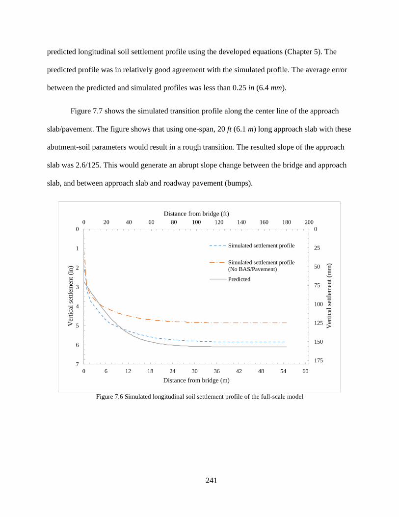
241
predicted longitudinal soil settlement profile using the developed equations (Chapter 5). The
predicted profile was in relatively good agreement with the simulated profile. The average error
between the predicted and simulated profiles was less than 0.25 in (6.4 mm).
Figure 7.7 shows the simulated transition profile along the center line of the approach
slab/pavement. The figure shows that using one-span, 20 ft (6.1 m) long approach slab with these
abutment-soil parameters would result in a rough transition. The resulted slope of the approach
slab was 2.6/125. This would generate an abrupt slope change between the bridge and approach
slab, and between approach slab and roadway pavement (bumps).
Figure 7.6 Simulated longitudinal soil settlement profile of the full-scale model
0 6 12 18 24 30 36 42 48 54 60
0
25
50
75
100
125
150
175
0
1
2
3
4
5
6
7
0 20 40 60 80 100 120 140 160 180 200
Distance from bridge (m)
Ver
tica
l se
ttle
men
t (m
m)
Ver
tica
l se
ttle
men
t (i
n)
Distance from bridge (ft)
Simulated settlement profile
Simulated settlement profile
(No BAS/Pavement)
Predicted

242
Figure 7.7 Simulated transition profile of the full-scale model
Using the information obtained from the results of the initial simulations, the size, length,
and spacing of piles, as well as number and length of the approach slab segments were
determined (using the procedure explained in section 6.2 and pile settlement design chart shown
in Figure 7.8). Accordingly, two approach slab segments were found to be sufficient to produce
the smooth transition as follows: (a) a slope of 1/125 of the first segment could be achieved using
30 ft (9.1 m) approach slab segment. (b) a second segment of 20 ft (6.1 m) long was found to be
sufficient such that 𝐿𝐵𝐴𝑆−𝐴 (1
125) < ∆𝑇≤ (𝐿𝐵𝐴𝑆−𝐴 + 𝐿𝐵𝐴𝑆−𝐵) (
1
125). (c) one pile line was used to
support the two segments. At that location, soil deformation (with no BAS/Pavement) was 4.3 in
(109 mm). Consequently, Rsett was estimated as 0.34.
Accordingly, load calculations were carried out to determine the size, length, and spacing
of piles in which provides the targeted Rsett. The pile line was assumed to support one-half of
BAS/Pavement
interface
0 6 12 18 24 30 36 42 48 54 60
0
25
50
75
100
125
150
175
0
1
2
3
4
5
6
7
0 20 40 60 80 100 120 140 160 180 200
Distance from bridge (m)
Ver
tica
l se
ttle
men
t (m
m)
Ver
tica
l se
ttle
men
t (i
n)
Distance from bridge (ft)
Simulated transition profile

243
each approach slab segment. Accordingly, it was found (using trial and error method) that pile
size of 18 in (457 mm), 45 ft (13.7 m) long, spaced at 8 ft (2.4 m) would be sufficient to carry the
estimated load of Q/Qu = 0.33 and provide the targeted Rsett = 0.34. Figure 7.8 shows the
determination of pile configuration using the pile settlement design chart developed for this pile-
soil conditions.
Figure 7.8 Determination of pile size and length
Figures 7.9 and 7.10 show the schematic layout of the proposed two-segment pile-
supported approach slab system. A pile cap of 3.0×2.5 ft ( 0.9×0.8 m) at top of pile line was
used. In the transverse direction, the piles were spaced 8 ft (2.4 m) center-to-center and were
distributed starting from the center of the approach slab toward the its edge. Three edge pile
spacing, Se-p, were used. The edge-pile (pile 6) was spaced at Se-p = 8 and 4.5 ft (2.4 and 1.4 m)
from pile 5. One configuration was also simulated with no edge-pile (without pile 6). The
0.1
0.2
0.3
0.4
0.5
0.6
0.00 0.10 0.20 0.30 0.40 0.50 0.60 0.70 0.80 0.90 1.00
Red
uct
ion o
f se
ttle
men
t (
Rse
tt)
Q/Qu
Pile settlement design chart
Dp=18in(457mm) Lp=35ft(10.7m)
Dp=18in(457mm) Lp=45ft(13.7m)
Dp=18in(457mm) Lp=55ft(16.8m)
Dp=12in(305mm) Lp=35ft(10.7m)
Dp=12in(305mm) Lp=45ft(13.7m)
Dp=12in(305mm) Lp=55ft(16.8m)
Dp=6in(152mm) Lp=35ft(10.7m)
Dp=6in(152mm) Lp=45ft(13.7m)
Dp=6in(152mm) Lp=55ft(16.8m)

244
anticipated pile head load, Q, was 39 kips (173 kN). Figures 7.11 and 7.12 show the finite
element discretization of the full-scale multi-segment pile supported approach slab system.
Figure 7.9 Longitudinal cross section of the proposed two-segment pile-supported approach slabs

245
Figure 7.10 Transverse cross section of the proposed two-segment pile-supported approach slabs
Figure 7.11 Finite element discretization of the full-scale with two-segment pile-supported approach slabs

246
Figure 7.12 Finite element discretization of piles and cap (a) Se-p = 8 ft (b) Se-p = 4.5 ft (c) No edge-pile
The nodes from the two approach slab segments were connected using shear coupling
connection. This connection was modeled to act as a joint in which restrains relative movement
while allows rotation between the two segments. In addition, the connection between the piles
and the pile cap was modeled as rigid connection.
The results from the simulations are presented below. Figures 7.13 and 7.14 show the
contour of the vertical deformation and excess pore pressure at the end of the analysis,
respectively.

247
Figure 7.13 Vertical deformation contour of the full-scale model with two-segment pile-supported approach slabs
(ft)
Figure 7.14 Excess pore pressure contour of the full-scale model with two-segment pile-supported approach slabs
(psf)
Figure 7.15 shows the simulated transition profile along the center line of the two
approach slab segments. The simulated two-segment pile-supported approach slabs performed
best (distribution of load among piles) when Se-p = 8 ft (2.4 m). The resulted slope of the
approach slab segments were 0.9/125 and 0.8/125, respectively.

248
Figure 7.15 Simulated transition profile of the full-scale model with two-segment pile-supported approach slabs
Figures 7.16, 7.17, and 7.18 show the pile axial load distribution for the three pile
configurations. The figures show that when no edge-pile was used, the outer piles (piles 4 and 5)
experienced greater axial load than anticipated. This was attributed to the load-stiffness behavior
developed among the piles. As the middle piles (piles 1,2, and 3) lost stiffness, due to settlement,
the load was transferred to the outer piles (piles 4 and 5). The axial load was reduced
considerably when an edge-pile was introduced (Figures 7.17 and 7.18). Figure 7.19 shows the
pile head settlement along the transverse direction for the three pile configurations. The figure
shows the variation in load-stiffness behavior among the piles as a function of pile spacing.
Ultimately, it can be concluded that pile configuration (a) (Figure 7.12) would perform the best
in a real-case scenario.
End of first BAS
End of second BAS
0 6 12 18 24 30 36 42 48 54 60
0
25
50
75
100
125
150
175
0
1
2
3
4
5
6
7
0 20 40 60 80 100 120 140 160 180 200
Distance from bridge (m)
Ver
tica
l se
ttle
men
t (m
m)
Ver
tica
l se
ttle
men
t (i
n)
Distance from bridge (ft)
Simulated transition profile

249
Figure 7.16 Axial load distribution in piles with Se-p = 8 ft
Figure 7.17 Axial load distribution in piles with Se-p = 4.5 ft
04590135180225270
0
1.5
3
4.5
6
7.5
9
10.5
12
13.5
15
0
10
20
30
40
50
0102030405060
Axial load (kN)
Pil
e d
epth
(m
)
Pil
e d
epth
(f
t)
Axial load (kips)
Axial load distribution in piles
Pile1
Pile2
Pile3
Pile4
Pile5
Pile6
04590135180225270
0
1.5
3
4.5
6
7.5
9
10.5
12
13.5
15
0
10
20
30
40
50
0102030405060
Axial load (kN)
Pil
e d
epth
(m
)
Pil
e d
epth
(f
t)
Axial load (kips)
Axial load distribution in piles
Pile1
Pile2
Pile3
Pile4
Pile5
Pile6

250
Figure 7.18 Axial load distribution in piles with no edge-pile
Figure 7.19 Pile heads settlement in the transverse direction
04590135180225270
0
1.5
3
4.5
6
7.5
9
10.5
12
13.5
15
0
10
20
30
40
50
0102030405060708090
Axial load (kN)
Pil
e d
epth
(m
)
Pil
e d
epth
(f
t)
Axial load (kips)
Axial load distribution in piles
Pile1
Pile2
Pile3
Pile4
Pile5
02.557.51012.515
0
25
50
75
0
1
2
3
081624324048
Longitudinal distance (m)
Ver
tica
l se
ttle
men
t (m
m)
Ver
tica
l se
ttle
men
t (i
n)
Longitudinal distance (ft)
Pile head settlement
Se-p = 8 ft
Se-p = 4.5 ft
No edge-pile

251
It is important to maintain the reaction forces on piles head (axial load). As live loads,
namely truck loads, could add a substantial amount of force when axle wheel load is directly on
the top of the pile head. This load, among others, shall be considered in the design stage to make
sure the capacity of the piles is sufficient.
Based on the results obtained from the full-scale simulation, recommendations regarding
the design of multi-segment pile-supported approach slabs were drawn as follows:
• Multi-segment pile-supported approach slabs can be an effective solution in cases
where significant soil settlements create rough transitions between the bridge and
the roadway pavement.
• Pile sizes, lengths, and spacings can be determined based on the recommended
settlement equations. For that, pile head settlement design charts were developed
for various pile-soil conditions.
• Along the transverse direction, piles shall be adequately spaced such that
reactions on pile heads are equally distributed to the extent possible. Stiffness-
load analyses could be conducted to determine possible transverse pile spacings.
• A joint should be provided between adjacent approach slab segments. This joint
can be saw-cut (partially), and rubber poured over the center of the pile cap. This
allows a crack to develop underneath the joint, and thus, would have the ability to
accommodate rotations (Figure 7.20).
• Non-corroding dowel bars should be provided between various approach slab
segments at the center of the slab thickness. This would help restrain the relative
movement between approach slab segments while allowing free rotation between
them (Figure 7.20).
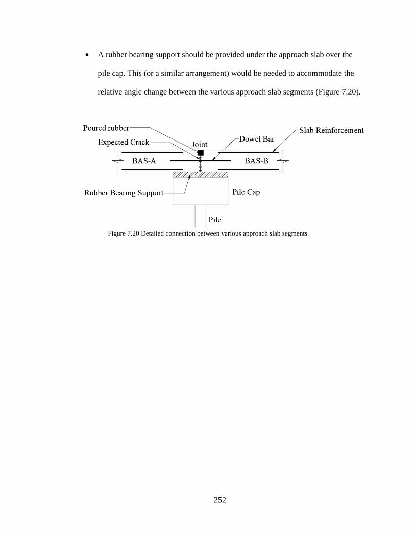
252
• A rubber bearing support should be provided under the approach slab over the
pile cap. This (or a similar arrangement) would be needed to accommodate the
relative angle change between the various approach slab segments (Figure 7.20).
Figure 7.20 Detailed connection between various approach slab segments

253
CHAPTER 8 - SUMMARY, CONCLUSIONS AND
RECOMMENDATIONS
The approach slab is an important element in the bridge approach system as it is intended
to provide riders with a smooth transition as their vehicle travels from the roadway to the bridge
and vice versa. In addition, the approach slab provides some protection to the bridge structural
elements from excessive truck dynamic impact. As soil underneath the approach slab settles,
deferential settlement develops between the bridge and the approaching roadway. This may
negatively affect the ride quality for travelers and result in substantial long-term maintenance
costs. Because of the differential settlement, bumps could develop at the ends of the bridge when
abrupt changes in slope (exceeding 1/125) occur (Figure 8.1) (Abu-Farsakh and Chen 2014,
Long, et al. 1999). The bump at the ends of the bridge is a well-known problem that affects 25%
of the bridges in the United States, resulting in an estimated $100 million per year in
maintenance expenditures (Briaud, James and Hoffman 1997).
Figure 8.1 Bump formation mechanism at the end of the bridge
This study was aimed at mitigating the formation of bumps at the end of the bridge
through a new design concept for the approach area. The proposed design takes advantage of
settlement-reducing piles that would support various approach slab segments and control their
254
settlement. These pile elements are intended to control the roughness of the transition such that
acceptable slope changes develop between various segments of the approach slab and thus
improve the performance of the approach slab system.
In this study, a comprehensive review of literature as well as a review of various state
practices regarding the approach area was performed. Information from the latest bridge design
manuals from various state departments of transportation were examined (Chapter 3). This
include the configuration of approach slab, connection of the approach slab to superstructure,
support type at the connection between the approach slab and pavement, backfill materials, and
side slope of the embankment fill. Data obtained from the bridge design manuals show that an
approach slab supported on a sleeper-slab resting on soil is mostly used. Furthermore, an
approach slab length of 15-30 ft (4.6-9.1 m) is commonly used.
A number of finite element models were developed, and parametric studies were
performed to evaluate the soil/approach slab settlement behind bridge abutments for various soil
conditions (Chapter 5), and to quantify the pile head settlement and load distribution along piles
as a function of pile-soil parameters (Chapter 6). From the results of these models, it is
concluded that an embankment fill height of greater than or equal to 20 ft ( 6.1 m) is more prone
to settlement issues in the transition zone. It has been determined that the degree of
compressibility of the embankment and natural soils, length of the approach slab, height of the
abutment, and height and side slope of the embankment influence the potential development of
bumps at approaches to bridges. Other factors such as the type of backfill material and the
erosion of backfill material were less significant and thus could be ignored when evaluating the
transition roughness.

255
Empirical relationships were developed that relate various soil parameters to the
longitudinal soil deformation profile behind bridge abutments . The effect of the abutment wall
on soil deformation soil was modelled using a logistic function (Figure 5.73). As a result, a set of
equations were developed that define the various parameters of the logistic function. Table 8.1
shows a summary of the developed equations. Definitions of the various parameters used in
Table 8.1 are given in Chapter 5.
Table 8.1 Summary of the developed equation of longitudinal settlement profile parameters
General form/parameters Developed equations
General form of the
logistic function
y = vertical settlement at a
distance of x from the
bridge abutment
y =𝑎
1 + 𝑏𝑒−𝑐𝑥
Logistic function
parameter (a)
Maximum displacement. 𝑎 = 383 × 10−6𝐻𝑛𝑒(27 𝜀𝑣
𝑒.𝑎𝑑𝑗+38.6 𝜀𝑣
𝑝) + 4980 × 10−6𝐻𝑒𝑒(61 𝜀𝑣
𝑒.𝑎𝑑𝑗.+23 𝜀𝑣
𝑝)
Logistic function
parameter (b)
Settlement at the interface
between the abutment wall
and the backfill soil.
𝑏 = 0.38 𝑙𝑛 (𝐶𝑐 ×𝐻𝑒
𝐻𝑎
) + 2.26
Logistic function
parameter (c)
Steepness of the curve.
𝑐 = 0.172e−0.182𝑎 *
𝑐 = 0.172e−0.007𝑎 **
* when (a) is in inches ** when (a) is in millimeters
Another set of finite element models was generated to quantify the pile-head settlement
as well as the load distribution along the pile for various pile-soil parameters/conditions (Chapter
6). Accordingly, design charts were developed such that pile-head settlement and the
corresponding reduction of settlement, Rsett could be determined for piles subjected to downdrag
forces based upon various soil conditions (Figures 6.16 through 6.18). Relationships were also
developed, using numerical analyses, to predict the distribution of axial load along the length of
the pile. This includes the neutral point, total downdrag force, positive skin friction, and end-

256
bearing. Table 8.2 shows a summary of the developed equations. The parameters shown in Table
8.2 are defined in Chapter 6.
Table 8.2 Summary of the developed pile head settlement/load distribution equations
Parameter Developed equations
Pile head settlement
ΔPH ∆𝑃𝐻= ∆𝑃𝑠 − 166
𝑄𝑑𝑑
𝐷𝑝𝐿𝑑𝑑𝐺𝑎𝑣𝑔−𝑑𝑑
+ 41𝑄
𝑝𝑠
𝐷𝑝𝐿𝑝𝑠𝐺𝑎𝑣𝑔−𝑝𝑠
+ 3.2𝑄
𝑏
𝐷𝑝2𝐸
𝑏
− 0.2
Neutral point
Ldd 𝐿𝑑𝑑 =
1 − [(𝑄𝑑𝑑@𝑄=0
− 𝑄𝑢) 𝐿𝑝
(𝐿𝑑𝑑@𝑄=0− 𝐿𝑑𝑑@𝑄𝑑𝑑=0
) 𝑄𝑢
(𝐿𝑑𝑑@𝑄𝑑𝑑=0
𝐿𝑝)] −
𝑄𝑄𝑢
(1 −𝑄𝑄𝑢
) [𝑄𝑑𝑑@𝑄=0
𝐿𝑝
𝐿𝑑𝑑@𝑄=0𝑄𝑢
] −(𝑄𝑑𝑑@𝑄=0
− 𝑄𝑢) 𝐿𝑝
(𝐿𝑑𝑑@𝑄=0− 𝐿𝑑𝑑@𝑄𝑑𝑑=0
) 𝑄𝑢
𝐿𝑝
Downdrag force
Qdd 𝑄𝑑𝑑 = (𝑄𝑢 − 𝑄) [
𝑄𝑑𝑑@𝑄=0𝐿𝑑𝑑
𝐿𝑑𝑑@𝑄=0𝑄𝑢
]
Positive skin friction
Qps 𝑄
𝑝𝑠= 𝑄 + 𝑄
𝑑𝑑− 𝑄
𝑢[𝑚3 + (
𝑄 + 𝑄𝑑𝑑
𝑄𝑢
) − 𝑚3 (𝐿𝑑𝑑
𝐿𝑝
)]
End-bearing
Qb 𝑄𝑏 = 𝑄𝑢 [𝑚3 + (
𝑄 + 𝑄𝑑𝑑
𝑄𝑢
) − 𝑚3 (𝐿𝑑𝑑
𝐿𝑝
)]
In addition, procedures were provided to estimate the length and number of approach slab
segments needed to achieve the desired transition profile (see Figure 8.2) as follows:
a) Determine the maximum longitudinal surface soil settlement, a or ∆𝑇, using either the
FEM analysis or the empirical equations provided in Chapter 5.
b) If ∆𝑇≤ 𝐿𝐵𝐴𝑆−𝐴 (1
125), use a single-segment approach slab with 𝐿𝐵𝐴𝑆−𝐴 ≤
30𝑓𝑡 (9.1𝑚). Minimize 𝐿𝐵𝐴𝑆−𝐴 to meet this requirement.
c) If ∆𝑇> 𝐿𝐵𝐴𝑆−𝐴 (1
125), the settlement cannot be accommodated with a single-segment
approach slab. Use a multi-segment pile-supported approach slab based on the
following procedures:

257
a. Select pile size, length, and pile spacing for the first line of piles such that the
expected pile head settlement ∆𝐴≤ 𝐿𝐵𝐴𝑆−𝐴 (1
125). Charts that can be used for
this estimation are given Chapter 6. If the desired ∆𝐴 cannot be achieved,
change 𝐿𝐵𝐴𝑆−𝐴, pile size, pile length, or pile spacing to satisfy the above
settlement requirement.
b. If 𝐿𝐵𝐴𝑆−𝐴 (1
125) < ∆𝑇≤ (𝐿𝐵𝐴𝑆−𝐴 + 𝐿𝐵𝐴𝑆−𝐵) (
1
125), try a two-segment
approach slab with one line of piles between the two segments. The end of the
second segment should be supported on a sleeper-slab on soil.
c. If ∆𝑇> (𝐿𝐵𝐴𝑆−𝐴 + 𝐿𝐵𝐴𝑆−𝐵) (1
125), the settlement cannot be accommodated
with a two-segment approach slab. Try a three-segment approach slab. The
end of the third segment should be supported on a sleeper-slab on soil.
d. Select the pile size, length, and pile spacing for the second line of piles (from
the charts) such that the expected pile head settlement ∆𝐴 + ∆𝐵≤
(𝐿𝐵𝐴𝑆−𝐴 + 𝐿𝐵𝐴𝑆−𝐵) (1
125).
e. If ∆𝑇> (𝐿𝐵𝐴𝑆−𝐴 + 2𝐿𝐵𝐴𝑆−𝐵 + 𝐿𝐵𝐴𝑆−𝐶) (1
125), the settlement cannot be
accommodated with a three-segment approach slab. Try four-segment
approach slab. The end of the fourth segment could be supported on a sleeper-
slab on soil.
f. Repeat steps a-e as needed.

258
Figure 8.2 Schematic of the proposed multi-segment pile-supported approach slab system
Ultimately, a full-scale simulation was conducted to verify the developed procedures and
relationships using a multi-segment pile-supported approach slab system (Chapter 7). The
number and length of the approach slab segments as well as the pile sizes, lengths and spacings
were estimated using the developed pile head settlement design charts.
Finally, the following conclusions can be made regarding the design of multi-segment
pile-supported approach slabs:
• Multi-segment pile-supported approach slabs can be an effective solution in cases
where significant soil settlements create rough transitions between the bridge and
the roadway pavement.

259
• Pile sizes, lengths, and spacings can be determined based on the recommended
settlement equations. For that, pile head settlement design charts were developed
for various pile-soil conditions.
• Along the transverse direction, piles shall be adequately spaced such that
reactions on pile heads are equally distributed to the extent possible. Stiffness-
load analyses could be conducted to determine possible transverse pile spacings.
• A joint should be provided between adjacent approach slab segments. This joint
can be saw-cut (partially), and rubber poured over the center of the pile cap. This
allows a crack to develop underneath the joint, and thus, would have the ability to
accommodate rotations (Figure 8.3).
• Non-corroding dowel bars should be provided between various approach slab
segments at the center of the slab thickness. This would help restrain the relative
movement between approach slab segments while allowing free rotation between
them (Figure 8.3).
• A rubber bearing support should be provided under the approach slab over the
pile cap. This (or a similar arrangement) would be needed to accommodate the
relative angle change between the various approach slab segments (Figure 8.3).
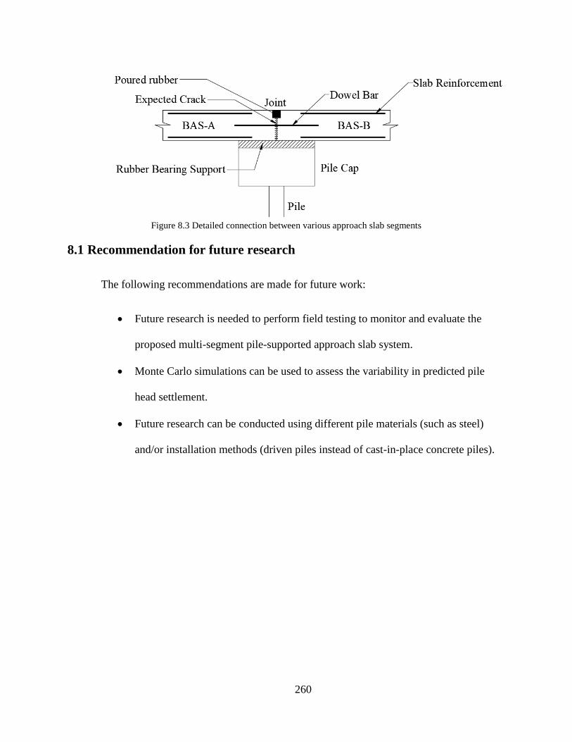
260
Figure 8.3 Detailed connection between various approach slab segments
8.1 Recommendation for future research
The following recommendations are made for future work:
• Future research is needed to perform field testing to monitor and evaluate the
proposed multi-segment pile-supported approach slab system.
• Monte Carlo simulations can be used to assess the variability in predicted pile
head settlement.
• Future research can be conducted using different pile materials (such as steel)
and/or installation methods (driven piles instead of cast-in-place concrete piles).

261
REFERENCES
AASHTO. 2001. A Policy on Geometric Design of Highways and Streets. AASHTO.
ABAQUS, Analysis User's Guide. 2015. Abaqus 2016 Online Documentation. Dassault
Systèmes, 2015.
Abu-Farsakh, Murad Y, and Qiming Chen. 2014. Field Demonstration of New Bridge Approach
Slab Designs and Performance. Baton Rouge, LA: Louisiana Transportation Research
Center.
Allen, David L, and Bobby W Meade. 1988. Soil-Bridge Abutment Interaction. Kentucky
Transportation Research Program, College of Engineering, University of Kentucky.
Ardani, A. 1987. Bridge approach settlement. Colorado Department of Highways, Report No.
CDOH-DTP-R-87-06.
Bakeer, Reda M, Mark A Shutt, Jianqiang Zhong, Sankar C Das, and Mark Morvant. 2005.
Performance of Pile-Supported Bridge Approach Slabs. American Society of Civil
Engineers.
Bakeer, Reda M, Mark A Shutt, Jianqiang Zhong, Sankar C Das, and Mark Morvant. 2005.
Performance of Pile-Supported Bridge Approach Slabs. Journal of Bridge Engineering,
Vol. 10, No. 2.
Bowles, Joseph E. 1997. Foundation analysis and design. McGraw-Hill.
Briaud, Jean Louis, and Yujin Lim. 1997. Soil-Nailed Wall Under Piled Bridge Abutment:
Simulation and Guidelines.

262
Briaud, Jean Louis, Ray W. James, and Stacey B. Hoffman. 1997. Synthesis of Highway Practice
234: Settlement of Bridge Approaches (The Bump at the end of the Bridges). Washington,
D.C.: Transportation Research Board, National Research Council.
Cai, C S, George Z Voyiadjis, and Xiaomin Shi. 2005. Determination of Interaction between
Bridge Concrete Approach Slab and Embankment Settlement. Baton Rouge, Louisiana:
Department of Civil Engineering, Louisiana State University.
Carter, Michael, and Stephen P Bentley. 2016. Soil properties and thier correlations (Second
edition). Wiley.
Coduto, Donald P. 2001. Foundation Design: Principles and Practices (Second Edition).
Prentice Hall.
Das, Baraja M. 2011. Principle of Foundation Engineering, Seventh Edition.
Das, Braja M. 2012. Fundamentals of Geotechnical Engineering, 4th Edition. CL Engineering.
Das, Sankar C, Reda Bakeer, Jianqiang Zhong, and Mark Schutt. 1999. Assessment of mitigating
embakment settlement with pile supported approach slabs. Civil and Environmental
Engineering Department, Tulane University.
Dupont, Bernadette, and David L Allen. 2002. Movements and Settlements of Highway Bridge
Approaches. Lexington, Kentucky: Kentucky Transportation Center.
Greimann, Lowell, Brent Phares, Adam Faris, and Jake Bigelow. 2008. Integral Bridge
Abutment-to-Approach Slab Connection. Ames, IA: Iowa Department of Transportation.
Helwany, Sam. 2007. Applied Soil Mechanics with ABAQUS Applications. Wiley.
263
Hopkins, Tommy C. 1985. Long-Term Movements of Highway Bridge Approach Embankments
and Pavements. Kentucky Transportation Center Research.
Hoppe, Edward J. 1999. Guidelines for the use, design, and construction of bridge approach
slabs. Charlottesville, Virginia: Virginia Transportation Research Council, VTRC 00-R4.
Hu, Yi Chin, Tsu Long Wu, Clyde E Lee, and Randy Machemhl. 1979. Roughness at the
Pavement-Bridge Interface, Research Number 213-1F. Texas State Department of
Highway and Public Transportation.
Irick, P E, and T L Copas. 1969. Bridge approach design and construction practices. NCHRP
Synthesis of Highway Practice 2, Highway Research Board.
Kramer, Steven L, and Peter Sajer. 1991. Bridge approach slab effectiveness. Washington State
Department of Transportation, Report No. WA-RD 227.1.
Laguros, J G, M M Zaman, and I U Mahmood. 1986. Evaluation of causes of excessive
settlements of pavement behind bridge abutments and their remedies-Phase I. Norman:
ODOT Study No. 84-12-2, Item 2140, ORA 155-857, University of Oklahoma.
Laguros, J G, M M Zaman, and I U Mahomood. 1990. Evaluation of Causes of Excessive
Settlements of Pavements Behind Bridge Abutments and their Remedies; Phase II. Rep.
No. FHWA/OK 89 (07), Oklahoma Department of Transportation.
Laguros, J G, M Zaman, Arumugam Alvappillai, and Kyriakos E Vavarapis. 1991. Evaluation of
Causes of Excessive Settlements of Pavements Behind Bridge Abutments and their
Remedies; Phase III. The University of Oklahoma.

264
Lenke, Lary R. 2006. Settlement Issues – Bridge Approach Slabs (Final Report Phase 1).
Transportation Engineering Research Program (TERP), Department of Civil Engineering,
University of New Mexico, Report No. NM04MNT-02.
Long, James H, Scott M Olson, Timothy D Stark, and Emile A Samara. 1999. Differential
movement at embankment - bridge structure interface in Illinois. Transportation Research
Record 1633, Paper No 98-1575.
McCarthy, David F. 2007. Essential of Soil Mechanics and Foundation, 7th edition. Pearson
Education, Limited.
McGrath, T. J., I. D. Moore, E. T. Selig, M. C. Webb, and B. Taleb. 2002. Recommended
Specifications for Large-Span Culverts. NCHRP Report 473, Transportation Research
Board, National Research Council.
McLaren, D. 1970. Settlement behind bridge abutments. The performance of silty clay fill in an
approach embankment on the M4 Motorway. RRL Reports, Road Res. Lab/UK/RRL
Dept., Lr 309.
Mistry, Vasant C. 2005. Integral Abutment and Jointless Bridges. Federal Highway
Administration.
Monley, Gregory J., and Jonathan T. H. Wu. 1993. TENSILE REINFORCEMENT EFFECTS ON
BRIDGE-APPROACH SETTLEMENT. Journal of Geotechnical Engineering.
Nabizadeh, Azam, Habib Tabatabai, and Mohammad A. Tabatabai. 2018. Survival Analysis of
Bridge Superstructures in Wisconsin. Applied Sciences, MDPI, 2018, 8, 2079.

265
Nassif, Hani, Talat Abu-Amra, and Nirali Shah. 2002. Finite Element Modeling of Bridge
Approach and Transition Slabs. New Jersey Department of Transportation, FHWA-NJ-
2002-007.
Nicks, Jennifer. 2015. "Bump at the Bridge." Long-Term Bridge Performance (LTBP) 5 (Federal
Highway Administration Research and Technology, FHWA-HRT-15-050): 8-9.
Phares, Brent, and Justin Dahlberg. 2015. Performance and design of bridge approach panels in
Wisconsin. Bridge Engineering Center, Iowa State University.
Puppala, Anand J, Sireesh Saride, Ekarut Archeewa, Laureano R Hoyos, and Soheil Nazarian.
2008. Recommendations for Design, Construction, and Maintenance of Bridge Approach
Slabs: Synthesis Report. Austin, Texas: Texas Department of Transportation, Research
and Technology Implementation Office.
Seo, Jeongbok, Hunsoo Ha, and Jean Louis Briaud. 2002. Investigation of Settlement at Bridge
Approach Slab Expansion Joint: Numerical Simulations and Model Tests. Austin, Texas:
Texas Department of Transportation, Research and Technology Implementation Office.
Tabatabai, Habib, and Azam Nabizadeh. 2018. Evaluation of Thin Polymer Overlays for Bridge
Decks. Proceeding of Structural Faults and Repair Conference, Edinburgh, UK.
Tabatabai, Habib, Azam Nabizadeh, and Mohammad A Tabatabai. 2018. Overview of Survival
Analysis Techniques for Probabilistic Assessment of Bridge Service Life. Proceeding of
Structural Faults and Repair Conference, Edinburgh, UK.

266
Wahls, Harvey E. 1990. Design and Construction of Bridge Approaches. Washington, D.C:
National Cooperative Highway Research Program, Synthesis of Highway Practice 159,
Transportation Research Board, National Research Council.
Walkinshaw, John L. 1978. Survey of Bridge Movements in the Western United States.
Washington, D.C., 6–12: Transportation Research Record 678: Tolerable Movements of
Bridge Foundations, Sand Drains, K-Test, Slopes, and Culverts, Transportation Research
Board, National Research Council.
Washington State Department of Transportation. 2015. Bridge Design Manula (LRFD), M23-
50.14. Engineering and Regional Operation, Bridge and Structure Office.
White, David, Sri Sritharan, Muhannad Suleiman, Mohamed Mekkawy, and Sudhar Chetlur.
2005. Identification of the Best Practices for Design, Construction, and Repair of Bridge
Approaches. Iowa Highway Research Board, Iowa Department of Transportation, CTRE
Project 02-118.
Wicke, M, and D Stoelhorst. 1982. Problems associated with the design and construction of
concrete pavements on approach embankments. Terminal House, Grosvenor Gardens,
London, England: Concrete Society.
Wong, H. K. W, and J C Small. 1994. Effect of Orientation of Bridge Slabs on Pavement
Deformation. Journal of Transportation Engineering, 120(4), 590–602.
Zaman, Musharraf , Giancarlo Gioda, and John Booker. 2000. Modeling in Geomechanics, 1st
Edition. Wiley.

267
APPENDICES
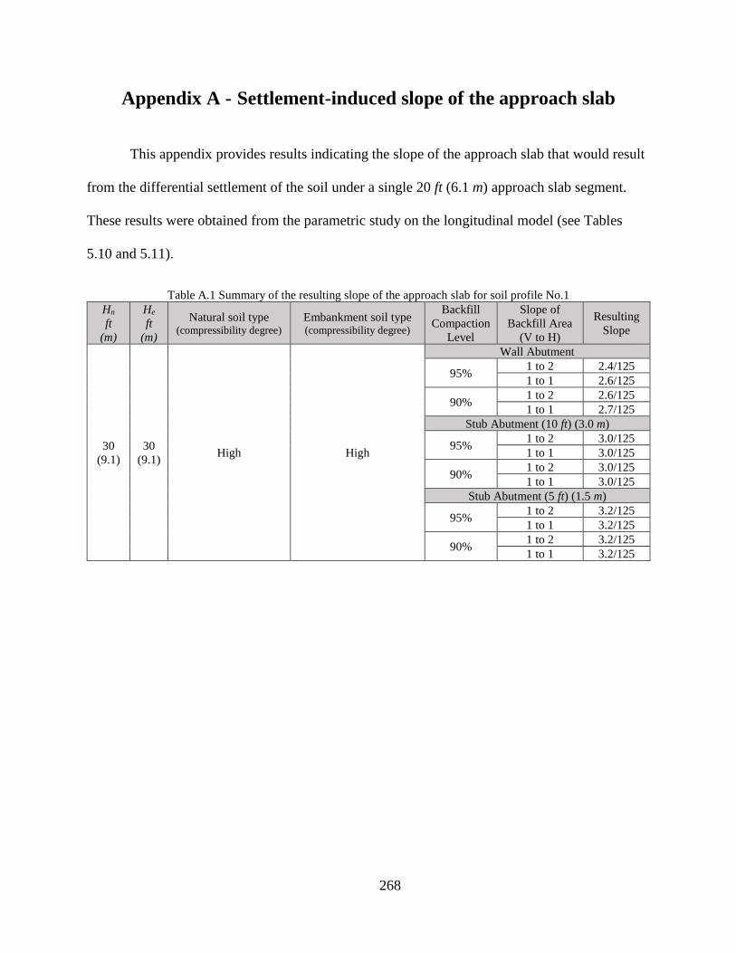
268
Appendix A - Settlement-induced slope of the approach slab
This appendix provides results indicating the slope of the approach slab that would result
from the differential settlement of the soil under a single 20 ft (6.1 m) approach slab segment.
These results were obtained from the parametric study on the longitudinal model (see Tables
5.10 and 5.11).
Table A.1 Summary of the resulting slope of the approach slab for soil profile No.1
Hn
ft
(m)
He
ft
(m)
Natural soil type (compressibility degree)
Embankment soil type (compressibility degree)
Backfill
Compaction
Level
Slope of
Backfill Area
(V to H)
Resulting
Slope
30
(9.1)
30
(9.1) High High
Wall Abutment
95% 1 to 2 2.4/125
1 to 1 2.6/125
90% 1 to 2 2.6/125
1 to 1 2.7/125
Stub Abutment (10 ft) (3.0 m)
95% 1 to 2 3.0/125
1 to 1 3.0/125
90% 1 to 2 3.0/125
1 to 1 3.0/125
Stub Abutment (5 ft) (1.5 m)
95% 1 to 2 3.2/125
1 to 1 3.2/125
90% 1 to 2 3.2/125
1 to 1 3.2/125

269
Table A.2 Summary of the resulting slope of the approach slab for soil profile No.2
Hn
ft
(m)
He
ft
(m)
Natural soil type (compressibility degree)
Embankment soil type (compressibility degree)
Backfill
Compaction
Level
Slope of
Backfill Area
(V to H)
Resulting
Slope
30
(9.1)
30
(9.1) High Moderate
Wall Abutment
95% 1 to 2 2.1/125
1 to 1 2.2/125
90% 1 to 2 2.1/125
1 to 1 2.2/125
Stub Abutment (10 ft) (3.0 m)
95% 1 to 2 2.3/125
1 to 1 2.3/125
90% 1 to 2 2.3/125
1 to 1 2.3/125
Stub Abutment (5 ft) (1.5 m)
95% 1 to 2 2.4/125
1 to 1 2.4/125
90% 1 to 2 2.4/125
1 to 1 2.4/125
Table A.3 Summary of the resulting slope of the approach slab for soil profile No.3
Hn
ft
(m)
He
ft
(m)
Natural soil type (compressibility degree)
Embankment soil type (compressibility degree)
Backfill
Compaction
Level
Slope of
Backfill Area
(V to H)
Resulting
Slope
30
(9.1)
30
(9.1) High Low
Wall Abutment
95% 1 to 2 1.9/125
1 to 1 1.9/125
90% 1 to 2 2.0/125
1 to 1 2.0/125
Stub Abutment (10 ft) (3.0 m)
95% 1 to 2 2.1/125
1 to 1 2.1/125
90% 1 to 2 2.1/125
1 to 1 2.1/125
Stub Abutment (5 ft) (1.5 m)
95% 1 to 2 2.1/125
1 to 1 2.1/125
90% 1 to 2 2.1/125
1 to 1 2.1/125

270
Table A.4 Summary of the resulting slope of the approach slab for soil profile No.4
Hn
ft
(m)
He
ft
(m)
Natural soil type (compressibility degree)
Embankment soil type (compressibility degree)
Backfill
Compaction
Level
Slope of
Backfill Area
(V to H)
Resulting
Slope
30
(9.1)
30
(9.1) Moderate Moderate
Wall Abutment
95% 1 to 2 1.3/125
1 to 1 1.4/125
90% 1 to 2 1.5/125
1 to 1 1.5/125
Stub Abutment (10 ft) (3.0 m)
95% 1 to 2 1.6/125
1 to 1 1.6/125
90% 1 to 2 1.6/125
1 to 1 1.6/125
Stub Abutment (5 ft) (1.5 m)
95% 1 to 2 1.7/125
1 to 1 1.7/125
90% 1 to 2 1.7/125
1 to 1 1.7/125
Table A.5 Summary of the resulting slope of the approach slab for soil profile No.5
Hn
ft
(m)
He
ft
(m)
Natural soil type (compressibility degree)
Embankment soil type (compressibility degree)
Backfill
Compaction
Level
Slope of
Backfill Area
(V to H)
Resulting
Slope
30
(9.1)
30
(9.1) Moderate Low
Wall Abutment
95% 1 to 2 1.3/125
1 to 1 1.4/125
90% 1 to 2 1.3/125
1 to 1 1.4/125
Stub Abutment (10 ft) (3.0 m)
95% 1 to 2 1.5/125
1 to 1 1.5/125
90% 1 to 2 1.5/125
1 to 1 1.5/125
Stub Abutment (5 ft) (1.5 m)
95% 1 to 2 1.5/125
1 to 1 1.5/125
90% 1 to 2 1.5/125
1 to 1 1.5/125

271
Table A.6 Summary of the resulting slope of the approach slab for soil profile No.6
Hn
ft
(m)
He
ft
(m)
Natural soil type (compressibility degree)
Embankment soil type (compressibility degree)
Backfill
Compaction
Level
Slope of
Backfill Area
(V to H)
Resulting
Slope
30
(9.1)
30
(9.1) Low Low
Wall Abutment
95% 1 to 2 1.2/125
1 to 1 1.3/125
90% 1 to 2 1.4/125
1 to 1 1.4/125
Stub Abutment (10 ft) (3.0 m)
95% 1 to 2 1.4/125
1 to 1 1.4/125
90% 1 to 2 1.4/125
1 to 1 1.4/125
Stub Abutment (5 ft) (1.5 m)
95% 1 to 2 1.4/125
1 to 1 1.4/125
90% 1 to 2 1.4/125
1 to 1 1.4/125
Table A.7 Summary of the resulting slope of the approach slab for soil profile No.7
Hn
ft
(m)
He
ft
(m)
Natural soil type (compressibility degree)
Embankment soil type (compressibility degree)
Backfill
Compaction
Level
Slope of
Backfill Area
(V to H)
Resulting
Slope
30
(9.1)
20
(6.1) High High
Wall Abutment
95% 1 to 2 1.1/125
1 to 1 1.2/125
90% 1 to 2 1.2/125
1 to 1 1.3/125
Stub Abutment (10 ft) (3.0 m)
95% 1 to 2 1.4/125
1 to 1 1.5/125
90% 1 to 2 1.5/125
1 to 1 1.5/125
Stub Abutment (5 ft) (1.5 m)
95% 1 to 2 1.6/125
1 to 1 1.6/125
90% 1 to 2 1.6/125
1 to 1 1.6/125
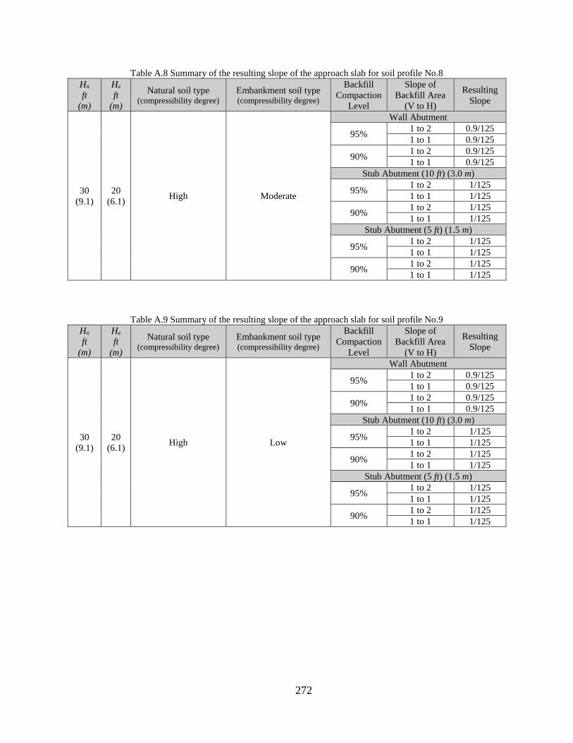
272
Table A.8 Summary of the resulting slope of the approach slab for soil profile No.8
Hn
ft
(m)
He
ft
(m)
Natural soil type (compressibility degree)
Embankment soil type (compressibility degree)
Backfill
Compaction
Level
Slope of
Backfill Area
(V to H)
Resulting
Slope
30
(9.1)
20
(6.1) High Moderate
Wall Abutment
95% 1 to 2 0.9/125
1 to 1 0.9/125
90% 1 to 2 0.9/125
1 to 1 0.9/125
Stub Abutment (10 ft) (3.0 m)
95% 1 to 2 1/125
1 to 1 1/125
90% 1 to 2 1/125
1 to 1 1/125
Stub Abutment (5 ft) (1.5 m)
95% 1 to 2 1/125
1 to 1 1/125
90% 1 to 2 1/125
1 to 1 1/125
Table A.9 Summary of the resulting slope of the approach slab for soil profile No.9
Hn
ft
(m)
He
ft
(m)
Natural soil type (compressibility degree)
Embankment soil type (compressibility degree)
Backfill
Compaction
Level
Slope of
Backfill Area
(V to H)
Resulting
Slope
30
(9.1)
20
(6.1) High Low
Wall Abutment
95% 1 to 2 0.9/125
1 to 1 0.9/125
90% 1 to 2 0.9/125
1 to 1 0.9/125
Stub Abutment (10 ft) (3.0 m)
95% 1 to 2 1/125
1 to 1 1/125
90% 1 to 2 1/125
1 to 1 1/125
Stub Abutment (5 ft) (1.5 m)
95% 1 to 2 1/125
1 to 1 1/125
90% 1 to 2 1/125
1 to 1 1/125
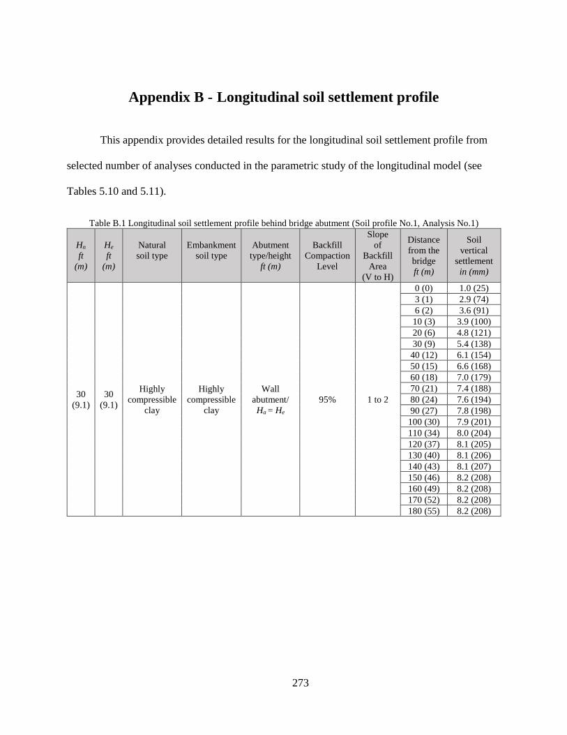
273
Appendix B - Longitudinal soil settlement profile
This appendix provides detailed results for the longitudinal soil settlement profile from
selected number of analyses conducted in the parametric study of the longitudinal model (see
Tables 5.10 and 5.11).
Table B.1 Longitudinal soil settlement profile behind bridge abutment (Soil profile No.1, Analysis No.1)
Hn
ft
(m)
He
ft
(m)
Natural
soil type
Embankment
soil type
Abutment
type/height
ft (m)
Backfill
Compaction
Level
Slope
of
Backfill
Area
(V to H)
Distance
from the
bridge
ft (m)
Soil
vertical
settlement
in (mm)
30
(9.1)
30
(9.1)
Highly
compressible
clay
Highly
compressible
clay
Wall
abutment/
Ha = He
95% 1 to 2
0 (0) 1.0 (25)
3 (1) 2.9 (74)
6 (2) 3.6 (91)
10 (3) 3.9 (100)
20 (6) 4.8 (121)
30 (9) 5.4 (138)
40 (12) 6.1 (154)
50 (15) 6.6 (168)
60 (18) 7.0 (179)
70 (21) 7.4 (188)
80 (24) 7.6 (194)
90 (27) 7.8 (198)
100 (30) 7.9 (201)
110 (34) 8.0 (204)
120 (37) 8.1 (205)
130 (40) 8.1 (206)
140 (43) 8.1 (207)
150 (46) 8.2 (208)
160 (49) 8.2 (208)
170 (52) 8.2 (208)
180 (55) 8.2 (208)

274
Table B.2 Longitudinal soil settlement profile behind bridge abutment (Soil profile No.1, Analysis No.12)
Hn
ft
(m)
He
ft
(m)
Natural
soil type
Embankment
soil type
Abutment
type/height
ft (m)
Backfill
Compaction
Level
Slope
of
Backfill
Area
(V to H)
Distance
from the
bridge
ft (m)
Soil
vertical
settlement
in (mm)
30
(9.1)
30
(9.1)
Highly
compressible
clay
Highly
compressible
clay
Stub
abutment/
Ha = 5 (1.5)
90% 1 to 1
0 (0) 1.3 (33)
3 (1) 3.5 (88)
6 (2) 4.4 (111)
10 (3) 5.0 (127)
20 (6) 6.0 (154)
30 (9) 6.5 (166)
40 (12) 7.0 (178)
50 (15) 7.3 (186)
60 (18) 7.6 (193)
70 (21) 7.8 (198)
80 (25) 7.9 (201)
91 (28) 8.0 (204)
101 (31) 8.1 (205)
111 (34) 8.1 (207)
121 (37) 8.2 (207)
131 (40) 8.2 (208)
141 (43) 8.2 (209)
151 (46) 8.2 (209)
161 (49) 8.2 (209)
171 (52) 8.2 (209)
180 (55) 8.2 (209)

275
Table B.3 Longitudinal soil settlement profile behind bridge abutment (Soil profile No.2, Analysis No.1)
Hn
ft
(m)
He
ft
(m)
Natural
soil type
Embankment
soil type
Abutment
type/height
ft (m)
Backfill
Compaction
Level
Slope
of
Backfill
Area
(V to H)
Distance
from the
bridge
ft (m)
Soil
vertical
settlement
in (mm)
30
(9.1)
30
(9.1)
Highly
compressible
clay
Moderately
compressible
clay
Wall
abutment/
Ha = He
95% 1 to 2
0 (0) 1.4 (36)
3 (1) 2.6 (67)
6 (2) 3.1 (80)
10 (3) 3.4 (87)
20 (6) 4.0 (102)
30 (9) 4.5 (114)
40 (12) 4.9 (125)
50 (15) 5.3 (134)
60 (18) 5.5 (140)
70 (21) 5.7 (145)
80 (24) 5.9 (149)
90 (27) 6.0 (152)
100 (30) 6.1 (154)
110 (34) 6.1 (156)
120 (37) 6.2 (157)
130 (40) 6.2 (158)
140 (43) 6.2 (158)
150 (46) 6.2 (159)
160 (49) 6.3 (159)
170 (52) 6.3 (159)
180 (55) 6.3 (159)

276
Table B.4 Longitudinal soil settlement profile behind bridge abutment (Soil profile No.2, Analysis No.12)
Hn
ft
(m)
He
ft
(m)
Natural
soil type
Embankment
soil type
Abutment
type/height
ft (m)
Backfill
Compaction
Level
Slope
of
Backfill
Area
(V to H)
Distance
from the
bridge
ft (m)
Soil
vertical
settlement
in (mm)
30
(9.1)
30
(9.1)
Highly
compressible
clay
Moderately
compressible
clay
Stub
abutment/
Ha = 5 (1.5)
90% 1 to 1
0 (0) 1.4 (36)
3 (1) 2.9 (73)
6 (2) 3.6 (92)
10 (3) 4.0 (102)
20 (6) 4.8 (121)
30 (9) 5.1 (129)
40 (12) 5.4 (136)
50 (15) 5.6 (142)
60 (18) 5.8 (147)
70 (21) 5.9 (150)
80 (25) 6.0 (153)
90 (28) 6.1 (154)
101 (31) 6.1 (156)
111 (34) 6.2 (157)
121 (37) 6.2 (158)
131 (40) 6.2 (159)
141 (43) 6.3 (159)
151 (46) 6.3 (159)
161 (49) 6.3 (160)
170 (52) 6.3 (160)
180 (55) 6.3 (160)

277
Table B.5 Longitudinal soil settlement profile behind bridge abutment (Soil profile No.3, Analysis No.1)
Hn
ft
(m)
He
ft
(m)
Natural
soil type
Embankment
soil type
Abutment
type/height
ft (m)
Backfill
Compaction
Level
Slope
of
Backfill
Area
(V to H)
Distance
from the
bridge
ft (m)
Soil
vertical
settlement
in (mm)
30
(9.1)
30
(9.1)
Highly
compressible
clay
Low
compressible
clay
Wall
abutment/
Ha = He
95% 1 to 2
0 (0) 1.5 (37)
3 (1) 2.4 (62)
6 (2) 2.9 (73)
10 (3) 3.1 (79)
20 (6) 3.6 (93)
30 (9) 4.0 (101)
40 (12) 4.3 (109)
50 (15) 4.5 (116)
60 (18) 4.7 (120)
70 (21) 4.8 (123)
80 (24) 4.9 (125)
90 (27) 5.0 (126)
100 (30) 5.0 (127)
110 (34) 5.0 (128)
120 (37) 5.0 (128)
130 (40) 5.1 (129)
140 (43) 5.1 (129)
150 (46) 5.1 (129)
160 (49) 5.1 (129)
170 (52) 5.1 (129)
180 (55) 5.1 (129)

278
Table B.6 Longitudinal soil settlement profile behind bridge abutment (Soil profile No.3, Analysis No.12)
Hn
ft
(m)
He
ft
(m)
Natural
soil type
Embankment
soil type
Abutment
type/height
ft (m)
Backfill
Compaction
Level
Slope
of
Backfill
Area
(V to H)
Distance
from the
bridge
ft (m)
Soil
vertical
settlement
in (mm)
30
(9.1)
30
(9.1)
Highly
compressible
clay
Low
compressible
clay
Stub
abutment/
Ha = 5 (1.5)
90% 1 to 1
0 (0) 2.1 (53)
3 (1) 3.0 (76)
6 (2) 3.3 (84)
10 (3) 3.5 (90)
20 (6) 4.1 (105)
30 (9) 4.3 (109)
40 (12) 4.5 (114)
50 (15) 4.6 (118)
60 (18) 4.8 (121)
70 (21) 4.8 (123)
80 (25) 4.9 (125)
90 (28) 5.0 (126)
101 (31) 5.0 (127)
111 (34) 5.0 (127)
121 (37) 5.0 (128)
131 (40) 5.1 (128)
141 (43) 5.1 (129)
151 (46) 5.1 (129)
161 (49) 5.1 (129)
170 (52) 5.1 (129)
180 (55) 5.1 (129)
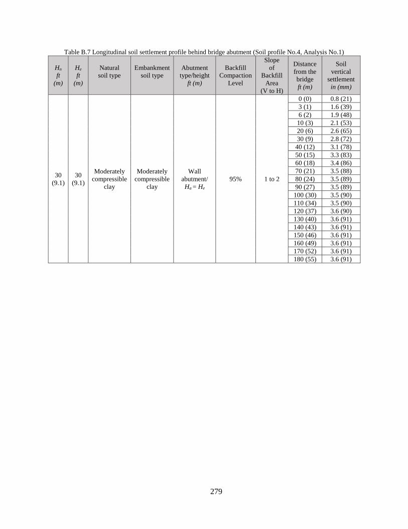
279
Table B.7 Longitudinal soil settlement profile behind bridge abutment (Soil profile No.4, Analysis No.1)
Hn
ft
(m)
He
ft
(m)
Natural
soil type
Embankment
soil type
Abutment
type/height
ft (m)
Backfill
Compaction
Level
Slope
of
Backfill
Area
(V to H)
Distance
from the
bridge
ft (m)
Soil
vertical
settlement
in (mm)
30
(9.1)
30
(9.1)
Moderately
compressible
clay
Moderately
compressible
clay
Wall
abutment/
Ha = He
95% 1 to 2
0 (0) 0.8 (21)
3 (1) 1.6 (39)
6 (2) 1.9 (48)
10 (3) 2.1 (53)
20 (6) 2.6 (65)
30 (9) 2.8 (72)
40 (12) 3.1 (78)
50 (15) 3.3 (83)
60 (18) 3.4 (86)
70 (21) 3.5 (88)
80 (24) 3.5 (89)
90 (27) 3.5 (89)
100 (30) 3.5 (90)
110 (34) 3.5 (90)
120 (37) 3.6 (90)
130 (40) 3.6 (91)
140 (43) 3.6 (91)
150 (46) 3.6 (91)
160 (49) 3.6 (91)
170 (52) 3.6 (91)
180 (55) 3.6 (91)

280
Table B.8 Longitudinal soil settlement profile behind bridge abutment (Soil profile No.4, Analysis No.12)
Hn
ft
(m)
He
ft
(m)
Natural
soil type
Embankment
soil type
Abutment
type/height
ft (m)
Backfill
Compaction
Level
Slope
of
Backfill
Area
(V to H)
Distance
from the
bridge
ft (m)
Soil
vertical
settlement
in (mm)
30
(9.1)
30
(9.1)
Moderately
compressible
clay
Moderately
compressible
clay
Stub
abutment/
Ha = 5 (1.5)
90% 1 to 1
0 (0) 1.4 (35)
3 (1) 1.9 (48)
6 (2) 2.4 (60)
10 (3) 2.7 (68)
20 (6) 3.2 (81)
30 (9) 3.3 (83)
40 (12) 3.4 (85)
50 (15) 3.4 (87)
60 (18) 3.5 (88)
70 (21) 3.5 (89)
80 (25) 3.5 (89)
90 (28) 3.5 (90)
101 (31) 3.5 (90)
111 (34) 3.6 (90)
121 (37) 3.6 (91)
131 (40) 3.6 (91)
141 (43) 3.6 (91)
151 (46) 3.6 (91)
161 (49) 3.6 (91)
170 (52) 3.6 (91)
180 (55) 3.6 (91)

281
Table B.9 Longitudinal soil settlement profile behind bridge abutment (Soil profile No.5, Analysis No.1)
Hn
ft
(m)
He
ft
(m)
Natural
soil type
Embankment
soil type
Abutment
type/height
ft (m)
Backfill
Compaction
Level
Slope
of
Backfill
Area
(V to H)
Distance
from the
bridge
ft (m)
Soil
vertical
settlement
in (mm)
30
(9.1)
30
(9.1)
Moderately
compressible
clay
Low
compressible
clay
Wall
abutment/
Ha = He
95% 1 to 2
0 (0) 0.9 (23)
3 (1) 1.5 (38)
6 (2) 1.8 (47)
10 (3) 2.0 (51)
20 (6) 2.4 (62)
30 (9) 2.6 (67)
40 (12) 2.8 (72)
50 (15) 3.0 (75)
60 (18) 3.0 (77)
70 (21) 3.1 (78)
80 (24) 3.1 (78)
90 (27) 3.1 (78)
100 (30) 3.1 (78)
110 (34) 3.1 (78)
120 (37) 3.1 (78)
130 (40) 3.1 (78)
140 (43) 3.1 (78)
150 (46) 3.1 (78)
160 (49) 3.1 (78)
170 (52) 3.1 (78)
180 (55) 3.1 (78)

282
Table B.10 Longitudinal soil settlement profile behind bridge abutment (Soil profile No.5, Analysis No.12)
Hn
ft
(m)
He
ft
(m)
Natural
soil type
Embankment
soil type
Abutment
type/height
ft (m)
Backfill
Compaction
Level
Slope
of
Backfill
Area
(V to H)
Distance
from the
bridge
ft (m)
Soil
vertical
settlement
in (mm)
30
(9.1)
30
(9.1)
Moderately
compressible
clay
Low
compressible
clay
Stub
abutment/
Ha = 5 (1.5)
90% 1 to 1
0 (0) 2.1 (54)
3 (1) 2.2 (57)
6 (2) 2.3 (59)
10 (3) 2.5 (63)
20 (6) 2.9 (73)
30 (9) 2.9 (74)
40 (12) 3.0 (76)
50 (15) 3.0 (77)
60 (18) 3.0 (77)
70 (21) 3.1 (78)
80 (25) 3.1 (78)
90 (28) 3.1 (78)
101 (31) 3.1 (78)
111 (34) 3.1 (78)
121 (37) 3.1 (78)
131 (40) 3.1 (78)
141 (43) 3.1 (78)
151 (46) 3.1 (78)
161 (49) 3.1 (78)
170 (52) 3.1 (78)
180 (55) 3.1 (78)

283
Table B.11 Longitudinal soil settlement profile behind bridge abutment (Soil profile No.6, Analysis No.1)
Hn
ft
(m)
He
ft
(m)
Natural
soil type
Embankment
soil type
Abutment
type/height
ft (m)
Backfill
Compaction
Level
Slope
of
Backfill
Area
(V to H)
Distance
from the
bridge
ft (m)
Soil
vertical
settlement
in (mm)
30
(9.1)
30
(9.1)
Low
compressible
clay
Low
compressible
clay
Wall
abutment/
Ha = He
95% 1 to 2
0 (0) 1.1 (27)
3 (1) 1.6 (39)
6 (2) 1.8 (47)
10 (3) 2.0 (51)
20 (6) 2.3 (60)
30 (9) 2.5 (63)
40 (12) 2.6 (66)
50 (15) 2.7 (69)
60 (18) 2.7 (70)
70 (21) 2.7 (70)
80 (24) 2.7 (70)
90 (27) 2.7 (69)
100 (30) 2.7 (69)
110 (34) 2.7 (69)
120 (37) 2.7 (69)
130 (40) 2.7 (69)
140 (43) 2.7 (69)
150 (46) 2.7 (69)
160 (49) 2.7 (69)
170 (52) 2.7 (69)
180 (55) 2.7 (69)

284
Table B.12 Longitudinal soil settlement profile behind bridge abutment (Soil profile No.6, Analysis No.12)
Hn
ft
(m)
He
ft
(m)
Natural
soil type
Embankment
soil type
Abutment
type/height
ft (m)
Backfill
Compaction
Level
Slope
of
Backfill
Area
(V to H)
Distance
from the
bridge
ft (m)
Soil
vertical
settlement
in (mm)
30
(9.1)
30
(9.1)
Low
compressible
clay
Low
compressible
clay
Stub
abutment/
Ha = 5 (1.5)
90% 1 to 1
0 (0) 2.1 (53)
3 (1) 2.2 (55)
6 (2) 2.3 (58)
10 (3) 2.4 (61)
20 (6) 2.7 (69)
30 (9) 2.7 (69)
40 (12) 2.7 (70)
50 (15) 2.8 (70)
60 (18) 2.8 (70)
70 (21) 2.7 (70)
80 (25) 2.7 (70)
90 (28) 2.7 (69)
101 (31) 2.7 (69)
111 (34) 2.7 (69)
121 (37) 2.7 (69)
131 (40) 2.7 (69)
141 (43) 2.7 (69)
151 (46) 2.7 (69)
161 (49) 2.7 (69)
170 (52) 2.7 (69)
180 (55) 2.7 (69)

285
Table B.13 Longitudinal soil settlement profile behind bridge abutment (Soil profile No.7, Analysis No.1)
Hn
ft
(m)
He
ft
(m)
Natural
soil type
Embankment
soil type
Abutment
type/height
ft (m)
Backfill
Compaction
Level
Slope
of
Backfill
Area
(V to H)
Distance
from the
bridge
ft (m)
Soil
vertical
settlement
in (mm)
20
(6.1)
20
(6.1)
Highly
compressible
clay
Highly
compressible
clay
Wall
abutment/
Ha = He
95% 1 to 2
0 (0) 0.1 (2)
3 (1) 1.0 (25)
6 (2) 1.3 (34)
10 (3) 1.6 (40)
20 (6) 2.2 (57)
30 (9) 2.6 (66)
40 (12) 2.9 (75)
50 (15) 3.2 (80)
60 (18) 3.3 (83)
70 (21) 3.3 (85)
80 (24) 3.4 (86)
90 (27) 3.4 (86)
100 (30) 3.4 (87)
110 (34) 3.4 (87)
120 (37) 3.4 (87)
130 (40) 3.4 (87)
140 (43) 3.4 (87)
150 (46) 3.4 (87)
160 (49) 3.4 (87)
170 (52) 3.4 (87)
180 (55) 3.4 (87)

286
Table B.14 Longitudinal soil settlement profile behind bridge abutment (Soil profile No.7, Analysis No.12)
Hn
ft
(m)
He
ft
(m)
Natural
soil type
Embankment
soil type
Abutment
type/height
ft (m)
Backfill
Compaction
Level
Slope
of
Backfill
Area
(V to H)
Distance
from the
bridge
ft (m)
Soil
vertical
settlement
in (mm)
20
(6.1)
20
(6.1)
Highly
compressible
clay
Highly
compressible
clay
Stub
abutment/
Ha = 5 (1.5)
90% 1 to 1
0 (0) 0.6 (16)
3 (1) 1.5 (37)
6 (2) 1.9 (48)
10 (3) 2.3 (57)
20 (6) 3.0 (75)
30 (9) 3.1 (79)
40 (12) 3.2 (82)
50 (15) 3.3 (84)
60 (18) 3.3 (85)
70 (21) 3.4 (86)
80 (25) 3.4 (86)
90 (28) 3.4 (87)
101 (31) 3.4 (87)
111 (34) 3.4 (87)
121 (37) 3.4 (87)
131 (40) 3.4 (87)
141 (43) 3.4 (87)
151 (46) 3.4 (87)
161 (49) 3.4 (87)
170 (52) 3.4 (87)
180 (55) 3.4 (87)

287
Table B.15 Longitudinal soil settlement profile behind bridge abutment (Soil profile No.8, Analysis No.1)
Hn
ft
(m)
He
ft
(m)
Natural
soil type
Embankment
soil type
Abutment
type/height
ft (m)
Backfill
Compaction
Level
Slope
of
Backfill
Area
(V to H)
Distance
from the
bridge
ft (m)
Soil
vertical
settlement
in (mm)
20
(6.1)
20
(6.1)
Highly
compressible
clay
Moderately
compressible
clay
Wall
abutment/
Ha = He
95% 1 to 2
0 (0) 0.3 (9)
3 (1) 0.9 (22)
6 (2) 1.1 (27)
10 (3) 1.2 (31)
20 (6) 1.7 (43)
30 (9) 1.9 (47)
40 (12) 2.0 (51)
50 (15) 2.1 (53)
60 (18) 2.1 (54)
70 (21) 2.1 (54)
80 (24) 2.2 (55)
90 (27) 2.2 (55)
100 (30) 2.2 (55)
110 (34) 2.2 (55)
120 (37) 2.2 (55)
130 (40) 2.2 (55)
140 (43) 2.2 (55)
150 (46) 2.2 (55)
160 (49) 2.2 (55)
170 (52) 2.2 (55)
180 (55) 2.2 (55)

288
Table B.16 Longitudinal soil settlement profile behind bridge abutment (Soil profile No.8, Analysis No.12)
Hn
ft
(m)
He
ft
(m)
Natural
soil type
Embankment
soil type
Abutment
type/height
ft (m)
Backfill
Compaction
Level
Slope
of
Backfill
Area
(V to H)
Distance
from the
bridge
ft (m)
Soil
vertical
settlement
in (mm)
20
(6.1)
20
(6.1)
Highly
compressible
clay
Moderately
compressible
clay
Stub
abutment/
Ha = 5 (1.5)
90% 1 to 1
0 (0) 0.8 (20)
3 (1) 1.1 (29)
6 (2) 1.4 (36)
10 (3) 1.6 (41)
20 (6) 2.0 (52)
30 (9) 2.1 (52)
40 (12) 2.1 (53)
50 (15) 2.1 (54)
60 (18) 2.1 (55)
70 (21) 2.2 (55)
80 (25) 2.2 (55)
90 (28) 2.2 (55)
101 (31) 2.2 (55)
111 (34) 2.2 (55)
121 (37) 2.2 (55)
131 (40) 2.2 (55)
141 (43) 2.2 (55)
151 (46) 2.2 (55)
161 (49) 2.2 (55)
170 (52) 2.2 (55)
180 (55) 2.2 (55)

289
Table B.17 Longitudinal soil settlement profile behind bridge abutment (Soil profile No.9, Analysis No.1)
Hn
ft
(m)
He
ft
(m)
Natural
soil type
Embankment
soil type
Abutment
type/height
ft (m)
Backfill
Compaction
Level
Slope
of
Backfill
Area
(V to H)
Distance
from the
bridge
ft (m)
Soil
vertical
settlement
in (mm)
20
(6.1)
20
(6.1)
Highly
compressible
clay
Low
compressible
clay
Wall
abutment/
Ha = He
95% 1 to 2
0 (0) 0.4 (10)
3 (1) 0.9 (23)
6 (2) 1.1 (29)
10 (3) 1.3 (33)
20 (6) 1.7 (43)
30 (9) 1.8 (47)
40 (12) 2.0 (50)
50 (15) 2.0 (51)
60 (18) 2.0 (52)
70 (21) 2.1 (52)
80 (24) 2.1 (52)
90 (27) 2.1 (52)
100 (30) 2.1 (52)
110 (34) 2.1 (52)
120 (37) 2.1 (52)
130 (40) 2.1 (52)
140 (43) 2.1 (52)
150 (46) 2.1 (52)
160 (49) 2.1 (52)
170 (52) 2.1 (52)
180 (55) 2.1 (52)

290
Table B.18 Longitudinal soil settlement profile behind bridge abutment (Soil profile No.9, Analysis No.12)
Hn
ft
(m)
He
ft
(m)
Natural
soil type
Embankment
soil type
Abutment
type/height
ft (m)
Backfill
Compaction
Level
Slope
of
Backfill
Area
(V to H)
Distance
from the
bridge
ft (m)
Soil
vertical
settlement
in (mm)
20
(6.1)
20
(6.1)
Highly
compressible
clay
Low
compressible
clay
Stub
abutment/
Ha = 5 (1.5)
90% 1 to 1
0 (0) 0.9 (24)
3 (1) 1.3 (33)
6 (2) 1.5 (37)
10 (3) 1.6 (40)
20 (6) 2.0 (50)
30 (9) 2.0 (50)
40 (12) 2.0 (51)
50 (15) 2.0 (52)
60 (18) 2.0 (52)
70 (21) 2.1 (52)
80 (25) 2.1 (52)
90 (28) 2.1 (52)
101 (31) 2.1 (52)
111 (34) 2.1 (52)
121 (37) 2.1 (52)
131 (40) 2.1 (52)
141 (43) 2.1 (52)
151 (46) 2.1 (52)
161 (49) 2.1 (52)
170 (52) 2.1 (52)
180 (55) 2.1 (52)

291
Appendix C - Pile-soil model results
This appendix provides detailed results for the pile head settlement, and load distribution
along the pile conducted in the parametric study of the pile-soil model (see Tables 6.2 and 6.3).
Table C.1 Pile head settlement and load distribution along the pile [Dp = 18 in (458 mm), Lp = 35 ft (10.7 m)]
Pile spacing
ft
(m)
Pile embedment length ΔPH
in
(mm)
Δs
in
(mm)
Q kips
(kN)
Qdd kips
(kN)
Ldd ft
(m)
Qps kips
(kN)
Qb kips
(kN)
Lb ft
(m)
Le ft
(m)
Ln ft
(m)
—
0.0 30.0
(9.1)
5.0
(1.5)
3.8
(97)
6.4
(163)
0.0 21.0
(93.2)
30.1
(9.2)
12.9
(57.3)
8.1
(35.9)
4.5
(1.4)
4.3
(110)
14
(60)
17.9
(79.6)
26.1
(7.9)
20.9
(93.2)
10.4
(46.5)
6.0
(1.8)
4.5
(113)
18
(80)
15.7
(70.0)
24.1
(7.3)
22.4
(99.8)
11.3
(50.3)
12.0
(3.7)
4.7
(120)
36
(160)
3.6
(15.9)
16.1
(4.9)
26.9
(119.4)
12.7
(56.6)
17 .0
(5.2)
4.9
(124)
51
(227) 0.0 0.0
37.3
(166.0)
13.7
(61.0)
—
12.0
(3.7)
18.0
(5.5)
3.4
(86)
5.9
(150)
0.0 20.0
(89.0)
29.1
(8.9)
12.5
(55.6)
7.5
(33.5)
4.5
(1.4)
3.7
(93)
14
(60)
16.2
(72.1)
25.1
(7.6)
20.3
(90.3)
9.4
(41.9)
6.0
(1.8)
3.8
(95)
18
(80)
13.6
(60.5)
24.1
(7.3)
21.9
(97.4)
9.7
(43.2)
12.0
(3.7)
3.9
(99)
36
(160) 0.0 0.0
25.8
(114.8)
10.2
(45.5)
17 .0
(5.2)
4.1
(103)
51
(227) 0.0 0.0
40.1
(178.4)
10.9
(48.5)
—
24.0
(7.3)
6.0
(1.8)
2.9
(73)
5.4
(137)
0.0 11.0
(48.8)
28.1
(8.6)
5.4
(24.0)
5.6
(24.8)
4.5
(1.4)
2.9
(75)
14
(60)
2.4
(10.7)
27.1
(8.3)
9.6
(42.5)
6.3
(28.2)
6.0
(1.8)
3.0
(75)
18
(80) 0.0 0.0
11.4
(50.8)
6.6
(29.3)
12.0
(3.7)
3.1
(78)
36
(160) 0.0 0.0
28.4
(126.3)
7.6
(33.8)
17 .0
(5.2)
3.4
(86)
51
(227) 0.0 0.0
41.3
(183.7)
9.7
(43.2)

292
Table C.2 Pile head settlement and load distribution along the pile [Dp = 18 in (458 mm), Lp = 45 ft (13.7 m)]
Pile spacing
ft
(m)
Pile embedment length ΔPH
in
(mm)
Δs
in
(mm)
Q kips
(kN)
Qdd kips
(kN)
Ldd ft
(m)
Qps kips
(kN)
Qb kips
(kN)
Lb ft
(m)
Le ft
(m)
Ln ft
(m)
—
0.0 30.0
(9.1)
15.0
(4.6)
3.6
(90)
6.4
(163)
0.0 30.8
(136.9)
36.1
(11.0)
21.0
(93.3)
9.8
(43.6)
4.5
(1.4)
3.7
(94) 14 (60)
23.2
(103.1)
33.1
(10.1)
26.3
(117.0)
10.4
(46.2)
6.0
(1.8)
3.8
(96) 18 (80)
21.9
(97.2)
31.1
(9.5)
29.2
(129.9)
10.7
(47.4)
12.0
(3.7)
4.3
(110) 36 (160)
17.5
(77.8)
26.1
(7.9)
39.2
(174.2)
14.3
(63.7)
17 .0
(5.2)
4.7
(119) 51 (227)
9.0
(40.0)
21.1
(6.4)
43.6
(194.2)
16.4
(72.7)
—
12.0
(3.7)
18.0
(5.5)
3.2
(80)
5.9
(150)
0.0 29.1
(129.5)
36.1
(11.0)
19.7
(87.8)
9.4
(41.7)
4.5
(1.4)
3.3
(84) 14 (60)
21.6
(96.2)
33.1
(10.1)
25.2
(112.3)
9.9
(44.0)
6.0
(1.8)
3.3
(85) 18 (80)
20.7
(92.2)
30.1
(9.2)
28.6
(127.4)
10.1
(44.9)
12.0
(3.7)
3.7
(94) 36 (160)
15.6
(69.4)
26.1
(8.0)
39.6
(176.0)
12.0
(53.6)
17 .0
(5.2)
3.9
(98) 51 (227)
4.5
(19.8)
22.1
(6.7)
42.4
(188.7)
13.0
(58.0)
—
24.0
(7.3)
6.0
(1.8)
2.8
(70)
5.4
(137)
0.0 27.5
(122.5)
37.1
(11.3)
18.5
(82.4)
9.0
(40.1)
4.5
(1.4)
2.9
(73) 14 (60)
18.3
(81.3)
34.1
(10.4)
22.4
(99.8)
9.3
(41.5)
6.0
(1.8)
2.9
(73) 18 (80)
15.0
(66.8)
31.1
(9.5)
23.6
(105.1)
9.4
(41.8)
12.0
(3.7)
3.0
(75) 36 (160)
3.7
(16.3)
28.1
(8.6)
30.0
(133.4)
9.7
(43.0)
17 .0
(5.2)
3.0
(77) 51 (227) 0.0 0.0
41.1
(182.8)
9.9
(44.2)

293
Table C.3 Pile head settlement and load distribution along the pile [Dp = 18 in (458 mm), Lp = 55 ft (16.8 m)]
Pile spacing
ft
(m)
Pile embedment length ΔPH
in
(mm)
Δs
in
(mm)
Q kips
(kN)
Qdd kips
(kN)
Ldd ft
(m)
Qps kips
(kN)
Qb kips
(kN)
Lb ft
(m)
Le ft
(m)
Ln ft
(m)
—
0.0 30.0
(9.1)
25.0
(7.6)
3.2
(81)
6.4 (163)
0.0 42.4
(188.6)
41.0
(12.5)
25.8
(114.9)
16.6
(73.6)
4.5
(1.4)
3.4
(86)
14
(60)
35.5
(158.1)
38.1
(11.6)
31.4
(139.7)
17.6
(78.4)
6.0
(1.8)
3.5
(88)
18
(80)
33.1
(147.1)
37.1
(11.3)
33.2
(147.5)
17.9
(79.6)
12.0
(3.7)
3.7
(93)
36
(160)
22.8
(101.5)
33.1
(10.1)
40.1
(178.4)
18.7
(83.2)
17 .0
(5.2)
4.0
(101)
51
(227)
19.7
(87.5)
28.1
(8.6)
50.8
(225.9)
19.9
(88.5)
—
12.0
(3.7)
18.0
(5.5)
2.9
(74)
5.9 (150)
0.0 41.6
(184.9)
41.0
(12.5)
26.2
(116.4)
15.4
(68.5)
4.5
(1.4)
3.1
(78)
14
(60)
34.3
(152.6)
38.1
(11.6)
31.4
(139.7)
16.4
(72.9)
6.0
(1.8)
3.1
(80)
18
(80)
31.4
(139.8)
37.1
(11.3)
32.8
(145.9)
16.6
(74.0)
12.0
(3.7)
3.3
(84)
36
(160)
21.2
(94.2)
31.1
(9.5)
39.8
(176.9)
17.4
(77.4)
17 .0
(5.2)
3.5
(89)
51
(227)
18.9
(83.9)
28.1
(8.6)
51.5
(229.1)
18.4
(81.6)
—
24.0
(7.3)
6.0
(1.8)
2.6
(65)
5.4 (137)
0.0 41.3
(183.7)
41.1
(12.5)
27.0
(120.0)
14.3
(63.7)
4.5
(1.4)
2.7
(69)
14
(60)
32.8
(145.7)
38.1
(11.6)
31.1
(138.5)
15.1
(67.3)
6.0
(1.8)
2.7
(70)
18
(80)
29.6
(131.6)
37.1
(11.3)
32.3
(143.5)
15.3
(68.1)
12.0
(3.7)
2.9
(73)
36
(160)
16.7
(74.5)
34.1
(10.4)
36.8
(163.8)
15.9
(70.7)
17 .0
(5.2)
2.9
(74)
51
(227)
6.8
(30.4)
28.1
(8.6)
41.6
(185.1)
16.2
(72.1)

294
Table C.4 Pile head settlement and load distribution along the pile [Dp = 12 in (305 mm), Lp = 35 ft (10.7 m)]
Pile spacing
ft
(m)
Pile embedment length ΔPH
in
(mm)
Δs
in
(mm)
Q kips
(kN)
Qdd kips
(kN)
Ldd ft
(m)
Qps kips
(kN)
Qb kips
(kN)
Lb ft
(m)
Le ft
(m)
Ln ft
(m)
—
0.0 30.0
(9.1)
5.0
(1.5)
4.2
(106)
6.4
(163)
0.0 13.9
(62.0)
30.1
(9.2)
8.0
(35.7)
5.9
(26.3)
3.0
(0.9)
4.4
(112)
9
(40)
11.1
(49.2)
25.1
(7.6)
12.3
(54.5)
7.8
(34.7)
6.0
(1.8)
4.6
(118)
18
(80)
5.9
(26.3)
20.1
(6.1)
14.9
(66.2)
9.0
(40.2)
—
12.0
(3.7)
18.0
(5.5)
3.4
(86)
5.9
(150)
0.0 13.5
(59.9)
29.1
(8.9)
8.1
(35.9)
5.4
(24.0)
3.0
(0.9)
3.7
(94)
9
(40)
10.3
(45.6)
24.1
(7.3)
12.4
(55.0)
6.9
(30.7)
6.0
(1.8)
3.8
(97)
18
(80)
3.0
(13.2)
21.1
(6.4)
13.9
(61.9)
7.1
(31.4)
—
24.0
(7.3)
6.0
(1.8)
2.8
(71)
5.4
(137)
0.0 8.3
(37.1)
28.1
(8.6)
4.6
(20.6)
3.7
(16.4)
3.0
(0.9)
2.9
(72)
9
(40)
2.4
(10.9)
27.1
(8.3)
7.2
(31.8)
4.3
(19.1)
6.0
(1.8)
2.9
(74)
18
(80) 0.0 0.0
13.1
(58.1)
4.9
(22.0)

295
Table C.5 Pile head settlement and load distribution along the pile [Dp = 12 in (305 mm), Lp = 45 ft (13.7 m)]
Pile spacing
ft
(m)
Pile embedment
length ΔPH
in
(mm)
Δs
in
(mm)
Q kips
(kN)
Qdd kips
(kN)
Ldd ft
(m)
Qps kips
(kN)
Qb kips
(kN) Lb ft
(m)
Le ft
(m)
Ln ft
(m)
—
0.0 30.0
(9.1)
15.0
(4.6)
3.6
(91)
6.4
(163)
0.0 19.9
(88.7)
35.1
(10.7)
12.9
(57.4)
7.0
(31.3)
3.0
(0.9)
3.7
(94)
9
(40)
14.9
(66.4)
32.1
(9.8)
16.5
(73.6)
7.4
(32.9)
6.0
(1.8)
4.0
(102)
18
(80)
13.4
(59.6)
28.1
(8.6)
22.6
(100.4)
8.8
(39.2)
12.0
(3.7)
4.7
(120)
36
(160)
3.8
(16.8)
18.1
(5.5)
28.1
(124.8)
11.7
(52.1)
—
12.0
(3.7)
18.0
(5.5)
3.2
(81)
5.9
(150)
0.0 19.2
(85.6)
36.1
(11.0)
12.4
(55.2)
6.8
(30.4)
3.0
(0.9)
3.3
(84)
9
(40)
14.2
(63.2)
31.1
(9.5)
16.2
(71.9)
7.0
(31.3)
6.0
(1.8)
3.5
(89)
18
(80)
12.7
(56.6)
28.1
(8.6)
22.9
(102.0)
7.8
(34.7)
12.0
(3.7)
3.9
(98)
36
(160)
0.7
(3.3)
20.1
(6.1)
27.1
(120.3)
9.7
(43.1)
—
24.0
(7.3)
6.0
(1.8)
2.7
(69)
5.4
(137)
0.0 18.4
(81.6)
36.1
(11.0)
11.7
(52.0)
6.7
(29.6)
3.0
(0.9)
2.8
(71)
9
(40)
12.8
(56.8)
30.1
(9.2)
15.0
(66.6)
6.8
(30.3)
6.0
(1.8)
2.8
(72)
18
(80)
6.8
(30.4)
28.1
(8.6)
18.0
(79.9)
6.9
(30.6)
12.0
(3.7)
2.9
(75)
36
(160) 0.0 0.0
29.0
(128.8)
7.1
(31.4)

296
Table C.6 Pile head settlement and load distribution along the pile [Dp = 12 in (305 mm), Lp = 55 ft (16.8 m)]
Pile spacing
ft
(m)
Pile embedment
length ΔPH
in
(mm)
Δs
in
(mm)
Q kips
(kN)
Qdd kips
(kN)
Ldd ft
(m)
Qps kips
(kN)
Qb kips
(kN) Lb ft
(m)
Le ft
(m)
Ln ft
(m)
—
0.0 30.0
(9.1)
25.0
(7.6)
3.4
(85)
6.4
(163)
0.0 27.4
(121.7)
40.0
(12.2)
15.9
(70.6)
11.5
(51.2)
3.0
(0.9)
3.5
(89)
9
(40)
22.9
(102.0)
37.1
(11.3)
19.8
(88.0)
12.1
(54.0)
6.0
(1.8)
3.6
(93)
18
(80)
17.7
(78.8)
34.1
(10.4)
23.1
(102.7)
12.6
(56.1)
12.0
(3.7)
4.2
(106)
36
(160)
10.9
(48.7)
26.1
(7.9)
32.8
(146.0)
14.1
(62.8)
—
12.0
(3.7)
18.0
(5.5)
2.9
(75)
5.9
(150)
0.0 27.2
(120.8)
40.1
(12.2)
16.1
(71.8)
11.0
(49.0)
3.0
(0.9)
3.1
(79)
9
(40)
22.4
(99.5)
37.1
(11.3)
19.9
(88.6)
11.4
(50.9)
6.0
(1.8)
3.2
(82)
18
(80)
16.5
(73.4)
35.1
(10.7)
22.8
(101.4)
11.7
(52.1)
12.0
(3.7)
3.6
(91)
36
(160)
9.7
(43.0)
27.1
(8.3)
32.7
(145.6)
12.9
(57.6)
—
24.0
(7.3)
6.0
(1.8)
2.6
(65)
5.4
(137)
0.0 27.3
(121.5)
40.1
(12.2)
16.8
(74.9)
10.5
(46.6)
3.0
(0.9)
2.7
(68)
9
(40)
21.7
(96.5)
37.1
(11.3)
19.8
(88.2)
10.9
(48.3)
6.0
(1.8)
2.8
(70)
18
(80)
15.6
(69.2)
35.1
(10.7)
22.5
(100.0)
11.1
(49.3)
12.0
(3.7)
2.9
(73)
36
(160)
3.6
(16.1)
28.1
(8.6)
28.3
(126.0)
11.3
(50.3)

297
Table C.7 Pile head settlement and load distribution along the pile [Dp = 6 in (152 mm), Lp = 35 ft (10.7 m)]
Pile spacing
ft
(m)
Pile embedment
length ΔPH
in
(mm)
Δs
in
(mm)
Q kips
(kN)
Qdd kips
(kN)
Ldd ft
(m)
Qps kips
(kN)
Qb kips
(kN) Lb ft
(m)
Le ft
(m)
Ln ft
(m)
—
0.0 30.0
(9.1)
5.0
(1.5)
4.2
(107)
6.4
(163)
0.0 6.9
(30.7)
29.1
(8.9)
3.5
(15.6)
3.4
(15.1)
1.5
(0.5)
4.5
(114)
5
(20)
5.3
(23.5)
24.1
(7.3)
5.4
(23.9)
4.4
(19.6)
3.0
(0.9)
4.7
(118)
9
(40)
2.5
(11.3)
18.1
(5.5)
6.8
(30.3)
4.7
(21.0)
—
12.0
(3.7)
18.0
(5.5)
3.4
(86)
5.9
(150)
0.0 6.7
(29.9)
29.1
(8.9)
3.6
(16.2)
3.1
(13.8)
1.5
(0.5)
3.7
(95)
5
(20)
4.8
(21.3)
23.1
(7.0)
5.5
(24.6)
3.8
(16.7)
3.0
(0.9)
3.8
(97)
9
(40)
1.1
(4.9)
21.1
(6.4)
6.2
(27.5)
3.9
(17.4)
—
24.0
(7.3)
6.0
(1.8)
2.9
(73)
5.4
(137)
0.0 5.6
(25.1)
28.1
(8.6)
3.4
(15.3)
2.2
(9.8)
1.5
(0.5)
2.9
(74)
5
(20)
2.0
(8.9)
27.1
(8.3)
3.9
(17.5)
2.6
(11.4)
3.0
(0.9)
3.0
(75)
9
(40) 0.0 0.0
6.2
(27.5)
2.8
(12.5)
Table C.8 Pile head settlement and load distribution along the pile [Dp = 6 in (152 mm), Lp = 45 ft (13.7 m)]
Pile spacing
ft
(m)
Pile embedment
length ΔPH
in
(mm)
Δs
in
(mm)
Q kips
(kN)
Qdd kips
(kN)
Ldd ft
(m)
Qps kips
(kN)
Qb kips
(kN) Lb ft
(m)
Le ft
(m)
Ln ft
(m)
—
0.0 30.0
(9.1)
15.0
(4.6)
3.6
(91)
6.4
(163)
0.0 10.0
(44.5)
35.1
(10.7)
5.9
(26.3)
4.1
(18.2)
1.5
(0.5)
3.7
(94)
5
(20)
7.5
(33.3)
32.1
(9.8)
7.7
(34.4)
4.3
(19.0)
3.0
(0.9)
4.1
(104)
9
(40)
6.4
(28.3)
27.1
(8.3)
10.4
(46.4)
4.9
(22.0)
—
12.0
(3.7)
18.0
(5.5)
3.2
(81)
5.9
(150)
0.0 9.6
(42.9)
35.1
(10.7)
5.8
(25.9)
3.8
(17.0)
1.5
(0.5)
3.3
(84)
5
(20)
7.1
(31.8)
31.1
(9.5)
7.6
(33.9)
4.0
(17.9)
3.0
(0.9)
3.6
(90)
9
(40)
6.1
(27.2)
27.1
(8.3)
10.7
(47.4)
4.5
(19.8)
—
24.0
(7.3)
6.0
(1.8)
2.8
(71)
5.4
(137)
0.0 9.1
(40.6)
35.1
(10.7)
5.6
(24.8)
3.6
(15.9)
1.5
(0.5)
2.9
(73)
5
(20)
7.0
(31.1)
30.1
(9.2)
7.8
(34.6)
3.7
(16.5)
3.0
(0.9)
2.9
(74)
9
(40)
4.3
(18.9)
28.1
(8.6)
9.4
(42.0)
3.8
(16.9)

298
Table C.9 Pile head settlement and load distribution along the pile [Dp = 6 in (152 mm), Lp = 55 ft (16.8 m)]
Pile spacing
ft
(m)
Pile embedment
length ΔPH
in
(mm)
Δs
in
(mm)
Q kips
(kN)
Qdd kips
(kN)
Ldd ft
(m)
Qps kips
(kN)
Qb kips
(kN) Lb ft
(m)
Le ft
(m)
Ln ft
(m)
—
0.0 30.0
(9.1)
15.0
(4.6)
3.4
(86)
6.4
(163)
0.0 13.1
(58.4)
39.0
(11.9)
7.5
(33.4)
5.6
(25.0)
1.5
(0.5)
3.6
(90)
5
(20)
10.9
(48.6)
36.1
(11.0)
9.6
(42.6)
5.8
(26.0)
3.0
(0.9)
3.7
(94)
9
(40)
8.4
(37.2)
33.1
(10.1)
11.3
(50.4)
6.0
(26.8)
—
12.0
(3.7)
18.0
(5.5)
3.0
(76)
5.9
(150)
0.0 13.0
(57.9)
40.0
(12.2)
7.6
(33.8)
5.4
(24.1)
1.5
(0.5)
3.2
(81)
5
(20)
10.7
(47.7)
36.1
(11.0)
9.7
(43.0)
5.6
(24.7)
3.0
(0.9)
3.3
(83)
9
(40)
7.9
(35.1)
33.1
(10.1)
11.2
(49.9)
5.7
(25.2)
—
24.0
(7.3)
6.0
(1.8)
2.6
(67)
5.4
(137)
0.0 13.2
(58.7)
39.1
(11.9)
7.9
(35.2)
5.3
(23.5)
1.5
(0.5)
2.8
(70)
5
(20)
10.6
(47.1)
36.1
(11.0)
9.7
(43.2)
5.4
(23.9)
3.0
(0.9)
2.9
(72)
9
(40)
7.5
(33.3)
33.1
(10.1)
11.1
(49.2)
5.4
(24.1)

299
CURRICULUM VITAE
Ahmed Zohuir Bahumdain
Place of birth: Jeddah, Saudi Arabia
Education:
B.S., King Abdulaziz University, May 2010
Major: Civil Engineering
M.S., University of Wisconsin-Milwaukee, May 2014
Major: Civil Engineering
Ph.D., University of Wisconsin-Milwaukee, May 2019
Major: Civil Engineering
Dissertation Title: Multi-Segment Pile-Supported Bridge Approach Slabs for Control of
Differential Settlement


![Pile Foundation Design[1] - ITDmtp.itd.co.th/ITD-CP/data/PileFoundationDesign.pdf · Introduction to pile foundations Pile foundation design Load on piles Single pile design Pile](https://img.dokumen.tips/doc/110x75/5a6ffb387f8b9ab1538b8376/pile-foundation-design1-itdmtpitdcothitd-cpdatapilefoundationdesignpdfpdf.jpg)