Multi-Objective Optimization of Complex Thermo … Optimization of Complex Thermo-Fluid Phenomena in Welding Agegnehu Atena Department of Mathematics Savannah State University Savannah,

International Journal of Applied Science and Technology Vol. 4 No. 1; January 2014

1

Multi-Objective Optimization of Complex Thermo-Fluid Phenomena in

Welding

Agegnehu Atena Department of Mathematics Savannah State University

Savannah, GA, 31404, USA

Abstract

This work is to investigate optimization of Gas metal arc welding (GMAW) by employing Multi Objective Optimization method. GMAW is a process that joins pieces of metal by heating them with an electric arc. The heat of the arc melts the surface of the base metal and the tip of the electrode. The electrode molten metal is transferred through the arc to the molten base metal to form the weld pool. The quality of the weld pool is characterized by the penetration depth, the bead height and width. These characteristics are controlled by a number of welding parameters. The subject of this paper is to establish the welding parameters that yield a weld pool which has a predefined geometry. The approach to this goal is by casting the problem of optimization of GMAW in the framework of Multi–Objective Optimization.

1. Introduction

Gas metal arc welding (GMAW) is a process used to join pieces of metal in the automotive manufacturing industry. In this process the pieces of metal are heated by an electric arc. The arc is between a continuously fed filler metal (consumable) electrode and the work piece. The heat of the arc melts the surface of the base metal and the tip of the electrode. The molten metal from the electrode is transferred through the arc to the molten base metal to form the weld pool. As the welding arc travels along the joint, the base metal is melted at the front edge of the pool, while it solidifies at the back edge. Externally supplied shielding gas protects the electrode and the weld pool from contamination. The GMAW process has become very popular in the last 40 years because of its speed and ease of use.

GMAW is a very complex process which is a result of interplay of different physical phenomena. This includes heat conduction with change of phase (melting and solidification of the metal in the weld pool); melting of the electrode, droplet formation, its detachment, and impingement onto the work piece; liquid–metal convection with free surfaces; surface–tension-driven convection (Marangoni effect); electromagnetic forces due to the presence of electromagnetic induction; interaction of the free surface with the arc plasma; and fluid flow in the weld pool [14],[2].The mathematical analysis and computational modeling of GMAW process are very difficult, because of the multi-physics involved and the multiscale (in time and space) complexity of the problem. The presence of free–boundaries also makes the problem more complex.

The quality of the weld joint is characterized by the penetration depth, the bead height and width. Weld penetration is the distance that the fusion line extends below the surface of the material being welded. These characteristics are controlled by a number of welding parameters. It is understood that the most important welding parameters in GMAW process are the welding current, arc length (the distance from the tip of the electrode to the work piece) and the arc travel speed (the rate that the arc moves along the work piece). These parameters will affect the weld pool characteristics to a great extent.

The welding current is associated to the amount of heat applied to the process and the weld pool penetration is directly related to the welding current. An increase or decrease in the current will increase or decrease the weld penetration respectively. As the arc length increases, the bead height decreases and bead width increases. The arc travel speed is the linear rate that the arc moves along the work piece. Welding speed affects both the width and penetration of the weld pool. With the lower speeds, too much metal is deposited in the base metal resulting in an increase in the weld pool height. At the higher speeds, the heat generated by the arc does not have sufficient time to substantially melt the base material resulting in a decrease in the weld pool height and width.

© Center for Promoting Ideas, USA www.ijastnet.com

2

The subject of this paper is to establish the welding parameters that yield a weld pool which has a predefined geometry. Our approach to this task is by casting the problem of optimization of GMAW in the framework of Multi–Objective Optimization. Gas–metal arc welding is a multi–input and multi–output process. Trial–and–error procedures have been used in the industry to identify key welding parameters in order to obtain a weld pool having desired characteristics. However, it is not only very expensive and time consuming, but also cannot provide the fundamental understanding of how the transport phenomena affect the weld quality. To overcome such difficulties, optimization procedures were developed to identify a proper set of process parameters that can produce the desired output of the gas arc welding process.

Optimization of input parameters in welding has remained an open research area. For example, Kim and Rhee [4] adopted the dual response approach to determine the parameters of the welding process which produce the target value with minimal variance. The dual response approach optimizes the penetration obtained in GMAW via the following procedure. First, the regression models of the mean value and standard deviation of the penetration are induced through the regression analysis. Next, an optimization algorithm based on these regression models and constraints is applied to determine the parameters which generate the desired penetration with minimized variance.

Kim et al. [3] conducted a sensitivity analysis of a robotic GMAW process to determine the effect of measurement errors on the uncertainty in estimated parameters. They employed non–linear multiple regression analysis for modeling the process and quantified the respective effects of process parameters on the geometry of the weld bead. Kim et al. [5] compared experimental data obtained for the weld bead geometry with those obtained from empirical formulae in gas–metal arc welding.

A bi–directional model of gas tungsten arc welding was developed in [8] by coupling a neural network model with a real number based genetic algorithm to calculate the welding conditions needed to obtain a target weld geometry. They showed that specific weld geometry was attainable via multiple path ways involving various sets of welding variables such as arc current, voltage and welding speed. While adjoint–based methods of PDE–constrained optimization [14] are well developed for thermo–fluid phenomena in welding process, it is too hard to apply such method to the current problem. In the present research effort the focus is on optimizing selected geometric parameters of the weld pool, namely the penetration depth, width and the height of the reinforcement track, see Fig. (2). Recognizing the conflicting nature of these objectives, we frame this problem in terms of multi–objective optimization which we believe should make it possible to identify the trade–offs inherent to these criteria.

All optimization methods require solution of the fluid flow and heat transfer equations performed several times in order to obtain one optimal solution. Therefore, it is imperative to make the flow solver as efficient as possible. To this end, we have parallelized the serial code using the OpenMP directives and have seen a considerable speedup of execution (the code acceleration will be measured as the ratio of the serial run time to the time required when the code is executed in parallel using N processors).

This paper is organized as follows. In Sec. II we formulate the set of partial differential equations, together with suitable boundary conditions, which describe the GMAW process. In Sec. III we introduce Multi–objective optimization and discuss how it is applied to GMAW process. Sec. IV contains results and discussion, whereas final conclusions are deferred to section V

2. Mathematical Modeling

The problem geometry is presented in section (2.1). Section (2.2) covers the governing equations used to describe the fluid flow and heat transfer in the problem, the droplet properties are discussed in section (2.3), the boundary conditions are given in section (2.4), and the last section (2.5) in this chapter is devoted for the discussion of the numerical methods used and some results.

2.1 Problem Geometry

We assume that the entire system is contained in a finite computational domain Ω ⊂R3. It is then subdivided into three subdomains Ω = ΩG ∪ ΩL ∪ ΩS, where ΩG is the region occupied by the plasma arc and the shielding gas, ΩL

denotes part of the domain that contains liquid phase from the melted electrode and melted work piece, and ΩS = ΩSE ∪ ΩSW refers to the solid region which is occupied by the unmelted electrode (ΩSE) and solid work piece (ΩSW). Fig. (1) shows the y - z cross-section of the computational domain. Between the liquid zone and solid zone, there is also a small zone called mushy zone where the liquid and solid metal coexist.


3

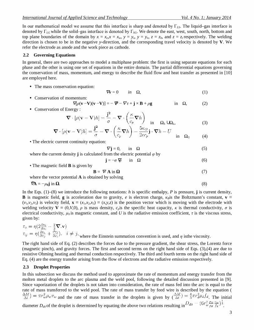
In our mathematical model we assume that this interface is sharp and denoted by ΓLS. The liquid–gas interface is denoted by ΓLG while the solid–gas interface is denoted by ΓSG. We denote the east, west, south, north, bottom and top plane boundaries of the domain by x = xe,x = xw, y = ys, y = yn, z = zb, and z = zt respectively. The welding direction is chosen to be in the negative y-direction, and the corresponding travel velocity is denoted by V. We refer the electrode as anode and the work piece as cathode.

2.2 Governing Equations

In general, there are two approaches to model a multiphase problem: the first is using separate equations for each phase and the other is using one set of equations in the entire domain. The partial differential equations governing the conservation of mass, momentum, and energy to describe the fluid flow and heat transfer as presented in [10] are employed here.

• The mass conservation equation: ∇·v = 0 in Ω, (1)

• Conservation of momentum: ∇·[ρ(v −V)(v −V)] = −∇P −∇· τ + j × B + ρg in Ω, (2)

• Conservation of Energy :

in ΩS ∪ ΩL, (3)

in ΩG (4) • The electric current continuity equation: ∇· j = 0, in Ω where the current density j is calculated from the electric potential φ by

(5)

j = −σ∇φ in Ω • The magnetic field B is given by

(6)

B = ∇× A in Ω where the vector potential A is obtained by solving

(7)

∇2A = −µ0j in Ω. (8)

In the Eqs. (1)–(8) we introduce the following notations: h is specific enthalpy, P is pressure, j is current density, B is magnetic field, g is acceleration due to gravity, e is electron charge, κBis the Boltzmann’s constant, v ≡ (v1,v2,v3) is velocity field, x ≡ (x1,x2,x3) ≡ (x,y,z) is the position vector which is moving with the electrode with welding velocity V ≡ (0,V,0), ρ is mass density, cpis the specific heat capacity, κ is thermal conductivity, σ is electrical conductivity, µ0 is magnetic constant, and U is the radiative emission coefficient, τ is the viscous stress, given by:

where the Einstein summation convention is used, and η isthe viscosity.

The right hand side of Eq. (2) describes the forces due to the pressure gradient, the shear stress, the Lorentz force (magnetic pinch), and gravity forces. The first and second terms on the right hand side of Eqs. (3),(4) are due to resistive Ohming heating and thermal conduction respectively. The third and fourth terms on the right hand side of Eq. (4) are the energy transfer arising from the flow of electrons and the radiative emission respectively.

2.3 Droplet Properties

In this subsection we discuss the method used to approximate the rate of momentum and energy transfer from the molten metal droplets to the arc plasma and the weld pool, following the detailed discussion presented in [9]. Since vaporization of the droplets is not taken into consideration, the rate of mass fed into the arc is equal to the rate of mass transferred to the weld pool. The rate of mass transfer by feed wire is described by the equation (

and the rate of mass transfer in the droplets is given by ( . The initial

diameter Dd0 of the droplet is determined by equating the above two relations resulting in .


4

Here, ∆M is a change in mass, ∆t is a change in time, rw is radius of the electrode wire, ρw is density of the wire, vwis wire feed rate, rd is radius of the droplet, ρdis density of the droplet, and fdis droplet transfer frequency. The droplet diameter Dd remains constant as the droplet falls through the arc region, but in the weld pool the droplet diameter is

, Where Din is the diameter on entering the weld pool, is the diameter at the previous axial control volume, and ∆z is the axial dimension of the current control volume. To describe the initial droplet velocity v0 ≡ (0,0,v0) (assuming that initially the horizontal components are zero), we have used the expression given in [7]. Lin et al. develops a simple expression for v0, based on the assumption that only the electromagnetic force is responsible for detachment, given by

Where G = 0.98 is a geometric factor. The droplet velocity, vd, in the arc is obtained by solving the equation of motion

, (9) Where md is the droplet mass, v is the plasma velocity, ρ is the plasma density, and is the drag coefficient. Integrating Eq. (9) over a small time interval ∆t, and assuming v is constant over the time interval, yields

v where t0 is the characteristic time.

The droplet velocity in the weld pool is given by

v

It is assumed that the droplet approaches the weld pool flow velocity exponentially, with a characteristic length equal to the droplet diameter as it enters the weld pool. The droplet temperature Td in the arc is obtained by solving the heat balance equation for the droplet,

) (10) over a small time interval ∆t

Where is the droplet density, Nu is the Nusselt number, Tdpis the droplet temperature at the start

of the time step, cpdis specific heat capacity of the droplet. The integration of Eq. (10) is performed under the assumption that the plasma temperature is constant over the time interval.

By assuming the droplet temperature approaches the weld pool temperature exponentially, with a characteristic length equal to the droplet diameter as it enters the weld pool, the droplet temperature in the weld pool is computed as

. Once we calculate the velocity and temperature of the droplet in the arc and the weld pool, we can determine the momentum and energy transfer of the molten droplet using Eqs. (11) and (12). The momentum transferred from the droplet to the arc and weld pool, per unit time, is given by

) (11) and the energy transferred is given by

) (12)


5

Wherein and out denote, respectively, the values entering and leaving the control volume. The momentum and energy transfers from the droplet to the arc plasma and weld pool are taken into account by adding Smin Eq. (2) and Se inEqs. (3) and (4) as a source term.

2.4 Boundary Conditions

At the east and west planes (x = xe,x = xw), the boundary conditions are v = 0,

∂Ai/∂x = 0, for i= 1,2,3, T = T0 = 300Kand ∂ϕ/∂x =0 At the south and north planes (y=ys , yn) v = 0, ∂Ai/∂y =0 for i= 1,2,3, T = T0 =300K, and∂ϕ/∂y=0 At the bottom plane (z= zt), v= 0,∂Ai/∂z =0 , for i= 1,2,3, ∂T/∂z =0 and φ = 0

At the top plane (z = zb)∂Ai/∂z =0 , for i= 1,2,3, T = T0 = 300K and

Where is the input current density and rais the radius of the electrode. The velocity boundary conditions take the form v1 = v2 = 0 with

Where Q is the input gas volumetric flow rate, r is the distance from the center of the electrode, rnozis the radius of the nozzle, , and

At the interface between the electrode and the plasma, and in the electrode itself v = 0. The term

, on ΓLS, (13)

is added on the right side of the energy equation, where the first term represents the heating effect of electrons absorbed at the anode, with the work function Φwa of the anode material, and the second term represents the radiative cooling of the anode. In Eq. (13), jcis the local current density, єais the emissivity of the anode, a is the Stefan–Boltzmann constant and Ta is the surface temperature of the anode. At the cathode–plasma interface, the term

, on ΓLS (14)

is added on the right side of the energy equation. In Eq. (14) the first term represents the heating effect of an electron emitted from the cathode less the energy required to emit an electron and the second term is the black body radiation loss. φcis the cathode voltage fall, ϕwc is the work function of the cathode material, jcis the local current density, and єcis emission coefficient.

The weld pool–plasma interface is subjected to the following free–surface boundary conditions:

Pp−Pw = −γ∇· n, on ΓLG, (15) τp−τw= −t · ∇sγ, on ΓLG, (16)

Where Ppand Pw are the pressures, respectively, on the plasma and weld pool sides of the interface,

(17)

is the curvature, τp and τw are the shear stress, respectively, on the plasma and weld pool sides, γ is the surface tension, t is a unit tangent vector, ∇s denotes tangential gradient, and h(x,y) is the surface height.

The most widely used methods for tracking of liquid surfaces are surface tracking methods such as volume–of–fluid (VOF) and the equilibrium surface method. We implemented the latter one. In this method, the weld pool surface profile is determined by assuming it has reached the equilibrium.


6

The weld pool free surface is calculated by minimizing the total surface energy taking into account the surface tension energy, the gravitational potential energy, and the work done by the arc force, Parc, and droplet impingement force Pd,

γK= ρgh+ Parc+ Pd+ λ,, on ΓLG, (18)

where λ is the Lagrange multiplier determined by a constraint representing the volume of the metal fed from the wire electrode. This constraint is given by

,

Where vw is wire feed speed, rwis the radius of the wire, and z0 is the height of the work piece before melting at a position ynthat is far enough behind the weld pool. The droplet pressure, Pd, on the free surface is calculated as

.

At the liquid–solid metal interface the term v is added on the right hand side of the momentum equation to account for the flow in the mushy zone. Here C and B are constants, and fl is fraction of liquids which is calculated as:

(19) Where Ts and Tl are, respectively, the solidus and liquidus temperatures. The latent heat of melting is taken into account by adding the source term

SH = ∇· [ρ(v −V)∆H]

to the energy equation, where H = h+∆H is the total enthalpy with the latent heat ∆H.

2.5 Numerical Methods

The numerical method used to solve the stationary conservation equations together with the appropriate boundary conditions is the control volume method of Patankar [13]. The general differential equation to be solved is expressed in the form ∇·(ρvΦ) = ∇·(ΓΦ∇Φ) + Sφ (20)

Whereρ is the fluid density, v is the velocity vector, ΓΦ is the diffusion coefficient, SΦ is a source term, and Φ represents a scalar variable (such as enthalpy, velocity component, etc.) to be solved. The computational domain is divided into small rectangular control volumes with a grid point at the center of each control volume storing the values of the variables. The discretized equation has the form [13]

aPΦP= aEΦE+ aWΦW+ aNΦN+ aSΦS+ aTΦT+ aBΦB+ SU∆V (21)

where the subscript P stands for a given grid point, while subscripts E, W, N, S, T, and B represents the east, west, north, south, top and bottom of the grid point P respectively. SU is the constant part of the source term SΦ which is expressed as SΦ = SU + SPΦP, and ∆V is the volume of the control volume. The coefficient aPis defined as:

aP= aE+ aW+ aN+ aS+ aT+ aB−SP∆V.

The discretized equations are solved by a combination of the tridiagonal matrix algorithm (TDMA), which provides a direct solution for the one–dimensional case, and the Gauss–Seidel point-by-point method.

3. Multi–Objective Optimization of GMAW Welding

In this Section we cast the problem of optimization of Gas Metal Arc Welding (GMAW) in the framework of Multi–Objective Optimization. Following a brief review of the main tenets of Multi–Objective Optimization, we will argue that this is in fact an appropriate setting for our problem and will show how GMAW optimization can be formulated in terms of Multi–Objective Optimization. We will also present some results of this approach.


7

3.1 Introduction to Multi–Objective Optimization

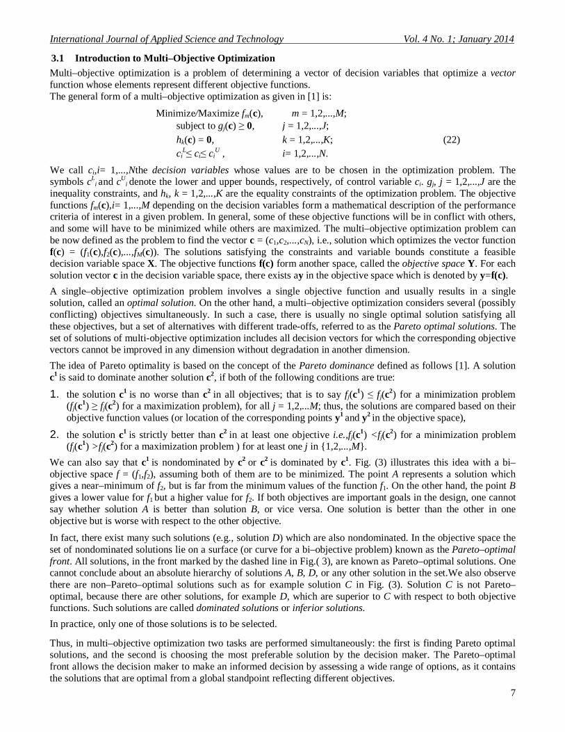
Multi–objective optimization is a problem of determining a vector of decision variables that optimize a vector function whose elements represent different objective functions. The general form of a multi–objective optimization as given in [1] is:

Minimize/Maximize fm(c), m = 1,2,...,M; subject to gj(c) ≥ 0, j = 1,2,...,J; hk(c) = 0, k = 1,2,...,K; (22) ci

L≤ ci≤ ciU , i= 1,2,...,N.

We call ci,i= 1,...,Nthe decision variables whose values are to be chosen in the optimization problem. The symbols cL

i and cUi denote the lower and upper bounds, respectively, of control variable ci. gj, j = 1,2,...,J are the

inequality constraints, and hk, k = 1,2,...,K are the equality constraints of the optimization problem. The objective functions fm(c),i= 1,...,M depending on the decision variables form a mathematical description of the performance criteria of interest in a given problem. In general, some of these objective functions will be in conflict with others, and some will have to be minimized while others are maximized. The multi–objective optimization problem can be now defined as the problem to find the vector c = (c1,c2,...,cN), i.e., solution which optimizes the vector function f(c) = (f1(c),f2(c),...,fM(c)). The solutions satisfying the constraints and variable bounds constitute a feasible decision variable space X. The objective functions f(c) form another space, called the objective space Y. For each solution vector c in the decision variable space, there exists ay in the objective space which is denoted by y=f(c).

A single–objective optimization problem involves a single objective function and usually results in a single solution, called an optimal solution. On the other hand, a multi–objective optimization considers several (possibly conflicting) objectives simultaneously. In such a case, there is usually no single optimal solution satisfying all these objectives, but a set of alternatives with different trade-offs, referred to as the Pareto optimal solutions. The set of solutions of multi-objective optimization includes all decision vectors for which the corresponding objective vectors cannot be improved in any dimension without degradation in another dimension.

The idea of Pareto optimality is based on the concept of the Pareto dominance defined as follows [1]. A solution c1 is said to dominate another solution c2, if both of the following conditions are true:

1. the solution c1 is no worse than c2 in all objectives; that is to say fj(c1) ≤ fj(c2) for a minimization problem (fj(c1) ≥ fj(c2) for a maximization problem), for all j = 1,2,...M; thus, the solutions are compared based on their objective function values (or location of the corresponding points y1 and y2 in the objective space),

2. the solution c1 is strictly better than c2 in at least one objective i.e.,fj(c1) <fj(c2) for a minimization problem (fj(c1) >fj(c2) for a maximization problem ) for at least one j in 1,2,...,M.

We can also say that c1 is nondominated by c2 or c2 is dominated by c1. Fig. (3) illustrates this idea with a bi–objective space f = (f1,f2), assuming both of them are to be minimized. The point A represents a solution which gives a near–minimum of f2, but is far from the minimum values of the function f1. On the other hand, the point B gives a lower value for f1 but a higher value for f2. If both objectives are important goals in the design, one cannot say whether solution A is better than solution B, or vice versa. One solution is better than the other in one objective but is worse with respect to the other objective.

In fact, there exist many such solutions (e.g., solution D) which are also nondominated. In the objective space the set of nondominated solutions lie on a surface (or curve for a bi–objective problem) known as the Pareto–optimal front. All solutions, in the front marked by the dashed line in Fig.( 3), are known as Pareto–optimal solutions. One cannot conclude about an absolute hierarchy of solutions A, B, D, or any other solution in the set.We also observe there are non–Pareto–optimal solutions such as for example solution C in Fig. (3). Solution C is not Pareto–optimal, because there are other solutions, for example D, which are superior to C with respect to both objective functions. Such solutions are called dominated solutions or inferior solutions.

In practice, only one of those solutions is to be selected.

Thus, in multi–objective optimization two tasks are performed simultaneously: the first is finding Pareto optimal solutions, and the second is choosing the most preferable solution by the decision maker. The Pareto–optimal front allows the decision maker to make an informed decision by assessing a wide range of options, as it contains the solutions that are optimal from a global standpoint reflecting different objectives.


8

Hence, optimizing multi–objective functions means finding such a solution which would give the values of all objective functions that is acceptable to the user.

3.2 Gas Metal Arc Welding as a Multi–Objective Optimization Problem

Gas metal arc welding is an arc welding process that uses a plasma arc between a continuous, consumable filler–metal electrode and the weld pool. Very complicated transport phenomena, including the arc plasma, electrode melting, and weld pool dynamics occur during the GMAW process. The fluid flow and heat transfer both in the arc and metal work piece affect the weld characteristics such as the weld penetration and the shape of the weld pool surface. When the electrode melts, droplets are formed and detached to be added to the weld pool, thereby raising the weld pool surface above the horizontal level (see Fig. ( 2)). The energy and momentum of droplets also increase the depth of the weld pool [9].

Gas metal arc welding is a multi–input and multi–output process. Trial–and–error procedures have been used in the industry to identify key welding parameters in order to obtain a weld pool having desired characteristics. However, it is not only very expensive and time consuming, but also cannot provide the fundamental understanding of how the transport phenomena affect the weld quality. To overcome such difficulties, optimization procedures were developed to identify a proper set of process parameters that can produce the desired output of the gas arc welding process.

In the present research effort we focus on optimizing selected geometric parameters of the weld pool, namely the penetration depth, the weld pool width, and the height of the reinforcement track (see Fig. (2)). Recognizing the conflicting nature of these objectives, we frame this problem in terms of multi–objective optimization which we believe should make it possible to identify the trade–offs inherent to these criteria. As regards the process control variables, we will use the wire feed rate, the welding speed, and the welding current, which will be discussed in more detail below.

3.2.1 The Process Control Variables

To obtain the desired weld pool geometry, it is essential to have a control over some essential parameters. Welding speed or travel speed controls the depth of penetration. Higher speeds reduce the penetration depth. If the welding speed is too slow, burn–through can occur which is an undesirable phenomenon in the welding process [12].

As arc lengths are increased, the arc voltage will increase, and the amperage will decrease. Arc voltage controls the width of the weld bead, with higher voltages generating wider beads.

The process also requires a sufficient electric current to melt both the electrode and a proper amount of base metal. The welding process must therefore be performed using a certain minimal amount of power (current) to achieve a required weld geometry and weld quality. The current density controls the depth of penetration, the higher the current density the greater the penetration. For example, if it is too high, the electrode will melt too fast and the molten weld pool will be too large.

Hence, the most important process control variables chosen for this study are the welding speed vw, the arc length Al, and the welding current I.

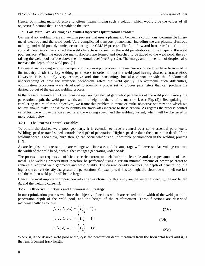
3.2.2 Objective Functions and Optimization Strategy

In our optimization process we chose the objective functions which are related to the width of the weld pool, the penetration depth of the weld pool, and the height of the reinforcement. These functions are described mathematically as follows

(23a)

(23b)

(23c)

Where b0 is the desired weld pool width, d0 is the penetration depth measured from the horizontal level and h0 is the reinforcement track height.


9

The symbols b(I,Al,vw), d(I,Al,vw) and h(I,Al,vw) denote the width, the penetration depth and reinforcement height obtained by solving the system of governing partial differential equations describing the fluid flow and heat transfer in the system corresponding to the current (I), the arc length(Al), and the travel speed(vw) (cf. [10], see also Fig. ( 2)). Thus, the goal we want to achieve in the optimization process is to produce a weld pool which has a width as close to the target width b0, with a penetration depth as close to d0 as possible, and having the reinforcement height as close to h0 as possible.

One of the most widely used methods for solving multi–objective optimization problems is to transform a multi–objective problem into a single objective problem. The weighted sum method is a method that parametrically changes the weights among the objective functions to obtain the Pareto–optimal front. The weight of an objective can be chosen in proportion to the relative importance of a given objective in the problem. Other applicable techniques include the –constraint method, weighted metric methods, and evolutionary methods to mention just a few.

The optimization strategy we adopt in our study is the weighted sum method. In this method, the individual objective functions are combined into one scalar objective function. For M objective functions, the aggregate objective function f is expressed as:

f(c) = w1f1(c) + w2f2(c) + ... + wMfM(c),

where x is the vector of the control variables, while f1,f2,...,fMare the individual scalar objective functions, and w1,w2,...,wMare the weights expressing the importance of each objective function in the optimization process. Usually, non–zero fractional weights are used and the sum of all weights is equal to one. The weight wi can be thought of as quantifying our desire to make fi small. Large value of wi indicates that we want the ith objective function small, if we consider fi less important we can take wi small. For example, if more emphasis is placed on obtaining a weld pool that has the desired penetration depth, then we will multiply the objective function related to the penetration depth by a weight that has larger value. Accordingly, the other objective functions will be multiplied by weights with lower values.

The weighted sum method can be employed as a posterior method, so that different weights are used to generate different Pareto–optimal solutions and then the decision maker selects the most satisfactory one. Alternatively, the decision maker can be asked to specify the weights in which case the method is used as an a priori method. We chose this method for its simplicity and it is one of the widely used methods to optimize multiple objectives simultaneously.

The scalar objective function to be minimized according to the optimization strategy described above is therefore

(24)

This formulation aims to optimize the single objective function f to obtain an optimal solution using a chosen weight vector (w1,w2,w3). To obtain different Pareto–optimal solutions, one can choose a different weight vector and optimize the resulting function f separately in each case. A resulting individual single–objective optimization problem has therefore the following form

minimize f(I,Al,vw) subject to (I,Al,vw) ∈R3

IL ≤ I ≤ IU (25) Al

L≤ Al ≤ AlU

vwL≤ vw≤ vw

U

3.2.3 Nonlinear Conjugate Gradient Method

In this study we use the Polak–Ribiere variant of the nonlinear conjugate gradient optimization algorithm [11] in order to solve problem (25). The optimization process is carried out iteratively in two steps. First, obtain the steepest descent direction and compute the conjugate direction via the Polak–Ribiere formula, and secondly, perform a line search procedure to determine the step size in the chosen direction.

Our implementation of the nonlinear conjugate gradient method is summarized by the following algorithm.


10

For simplicity of notation, the vector x = (x1,x2,x3) will denote the vector of the decision variables (I,Al,vw), whereas the vector (y1,y2,y3) will represent the vector of the system outputs (b,d,h).

Given x0: evaluate∇f(x0) start in the steepest descent direction: ∆x0 = −∇f(x0) find a step size α that minimizes f:

α0 = argminf(x0 + α∆x0) α

define : Λx0 = ∆x0 n ← 1

repeat calculate the steepest direction : ∆xn= −∇f(xn)

compute β using Polak-Ribiere formula :

update the conjugate direction : Λxn= ∆xn+ βnΛxn−1perform line minimization to find the step size αn:

αn= argminf(xn+ αΛxn) α

(The line search is performed using the Brent’s method) update the vector:xn+1 = xn+ αnΛxn n← n + 1

until a stopping criterion is satisfied

In the above algorithm the gradient ∇f(xn) of the scalar objective function Eq. (24) is given by

,

where the partial derivatives are computed using a finite difference approximation as,

fori,j =,1,2,3,

in which δxjis a small increment to the jth decision variable, and ej is the unit vector in the jth direction. The function values yi(xn) or yi (xn+ δxiei), are obtained by solving the entire system of governing equations describing the fluid flow and heat transfer using the corresponding input parameters.

4. Results and Discussion

In this section we present some results obtained by the multi–objective weighted sum method. Table (1) shows various combinations of the decision variables, i.e., arc current I, welding speed vw, the arc length Al obtained to achieve the target weld dimensions: penetration depth d0 = 1.9mm, reinforcement height h0 = 1.4mm, and weld pool width b0 = 5.9mm. Each row in the table is computed using different combinations of weights. We observe that several combinations of the decision variables produce a weld pool with similar dimension that indicates the existence of alternate paths to obtain the target weld geometry.

Multi–objective optimization is conducted in order to present trade–off information to the decision makers that enable them to make the best decision. In two-dimensional case, it is not difficult to interpret a Pareto curve that contains the optimal solutions. In three–dimensions, however, construction of the Pareto surface, with optimal solutions on it, is a bit difficult and we only plotted the optimal solutions.


11

Fig. (4) depicts the Pareto optimal solutions obtained using multi–objective weighted sum method. Note that some of the solutions are obtained by multiple combinations of the decision variables as shown in table (1).

The resulting flow patterns and temperature distributions, for selected optimal solutions, are shown in Fig. (5) in different cross–sections. Fig . (5a, 5b) display the flow solution where the objective function corresponding to the reinforcement height J3 is minimal (point B on Fig. (4)), i.e., the solution that gives a better approximation for the reinforcement height. The closest value, achieved in our simulation, to the desired reinforcement height h0 = 1.4mm is h = 1.31655 mm. However, this optimal solution does not give a good approximation for the penetration depth, i.e., the objective function corresponding to the penetration depth J2 is not minimal. This flow pattern is obtained using the welding current I = 95 A, the welding speed vw= −1.5 cm/s, and the arc length Al = 0.5cm.

Figs. (5c, 5d) show the optimal solution (point A on Fig. (4)) which have a good approximation for the penetration depth (the objective function J2 is minimal). The penetration depth d = 2.3177 mm is the nearest value to the desired depth ofd0 = 1.9 mm. This solution corresponds to the welding current I = 95.02702 A, welding speed vw= −1.47217 cm/s, and the arc length Al = 0.47298.

References

J. Branke, K. Deb, K. Miettinen, R. Slowinski (2008). Multi–objective Optimization: Interactive and Evolutionary Approaches. Springer–Verlag.

J. Hu, H. L. Tsai and P. C. Wang (2006). Numerical Modeling of GMAW arc. Advances in Computer, Information , and Systems Sciences, and Engineering, 69–74.

I .S. Kim, Y. J. Jeong, I. J. Son, I. J. Kim, J. Y. Kim, I. K.Kim, P. K. Yarlagadda (2003). Sensitivity analysis for process parameters influencing weld quality in robotic GMA welding process.J Mater Process Technol, 140.

D. Kim and S. Rhee (2003). Optimization of GMA welding process using the dual response approach.International journal of production research, 41.

I. S. Kim, K. J. Son, Y. S. Yang, P. K. Yarlagadda (2003). Sensitivity analysis for process parameters in GMA welding processes using a factorial design method.Int J Mach Tools Manuf, 43 .

C. H. Kim, W. Zhang and T. DebRoy (2003). Modeling of temperature field and solidified surface profile during gas–metal arc fillet welding. J. Appl. Phys., 94, No. 4.

Q. Lin, X, Li and S. Simpson (2001). Metal transfer measurments in gas metal arc welding. J. Phys. D: Appl. Phys.34, 347–353 .

S. Mishra and T. DebRoy (2007). Tailoring gas tungsten arc weld geometry using a genetic algorithm and a neural network trained with convective heat flow calculations. Materials Science and Engineering A, 454–455, 477–486

A. B. Murphy (2009). Modelling of Gas Metal Arc Welding of Aluminium, Stage2.3: Effect of Metal Droplets, Report CMSE,

A. B Murphy (2010). Modelling of Gas Metal Arc Welding of Aluminium, Stage2.2: Moving Arc with Molten Weld Pool. Report CMSE, .

J. Nocedal and S. Wright (2002). Numerical Optimization.Springer. P. K. Palani and N. Murugan (2007). Modelling and simulation of wire feed rate for steady current and pulsed

current gas metal arc welding using 317L flux cored wire. Int.J. ManufTechnol, 34, 1111-1119. S. V. Patankar (1980). Numerical Heat Transfer and Fluid Flow (1st ed.). Hemisphere Series on Computational

Methods in Mechanics and Thermal Science. Washington DC. O. Volkov, B. Protas, W. Liao and D. Glander( 2009). Adjoint–Based Optimization of Thermo–Fluid Phenomena

in Welding Processes. Journal of Engineering Mathematics, 65, 201–220,.


12

sy=y y=y

n

Figure 1: A section of the computational domain in the y −z plane.

Figure 2: The parameters defining the weld pool geometry: b is the width of the weld pool, h is the reinforcement height, and d is the penetration depth.

Ω G

z=z z

y

Ω

SE

t z=z

V

L

b

Ω SG

LG

Ω

LS

SG

SW


13

I (A) Al (cm) vw(cm/s) b (mm) d (mm) h (mm)

Table 1: Various combinations of welding variables: arc current I, welding speed vw, and arc length Al to achieve the weld pool dimensions: weld pool width b, penetration depth d, and reinforcement height h.

Figure 3: Schematic of a Pareto front together with some Pareto-optimal(A, B, and D) and dominated (C) solutions. Only two objective functions are considered.


14

Figure 4: Pareto optimal solutions (•) obtained by multi-objective weighted sum method. The points marked by ×, o, and *represent the projections of the Pareto solutions on the y - z, x - z and x - y planes, respectively. J1, J2, and J3 are, respectively, the objective functions corresponding to weld pool width, penetration depth, and reinforcement height.

(a) (b)

Figure 5: The temperature and velocity fields at y = 1:0 cross-section ( 5(a), 5(c)), andatx = 0 cross-section (5(b), 5(d)). The undisturbed weld pool surface is located atz = 30:1mm

0

1

2 x 10 −3

0 0.02 0.04 0.06 0.08 0.1

0

0.005

0.01

0.015

J2 J1

J3

A

B

C

Documents

Multi-Objective Optimization of Complex Thermo … Optimization of Complex Thermo-Fluid Phenomena in Welding Agegnehu Atena Department of Mathematics Savannah State University Savannah,