Multi-Objective Optimization and Multi-Criteria Decision MakingFor FDM Using Evolutionary Approaches

Nikhil Padhye, Subodh Kalia and Kalyanmoy Debnpdhye@gmail.com, subodh@iitk.ac.in, deb@iitk.ac.in

Department of Mechanical EngineeringIndian Institute of Technology Kanpur, Kanpur-208016, U.P., India

KanGAL Report 2009007

December 24, 2009

Abstract

In this paper, we describe a systematic multi-objective problem solving approach, simulataneoslyminimizing two conflicting goals - average surface roughness ‘Ra’ and build time ‘T ’, for object manu-facturing in FDM process by usage of evolutionary algorithms. Popularly used multi-objective geneticalgorithm NSGA-II and recently proposed multi-objective particle swarm optimization (MOPSO) al-gorithms, are employed for the optimization purposes. Statistically significant performance measuresare employed to compare the two algorithms and means to arrive at approximate Pareto-optimal frontsare also suggested. To refine the solutions obtained by the optimizers, a mutation driven hill climbinglocal search is also proposed. Several suggestions and three new proposals pertaining to the issue ofdecision making in presence of trade-off solutions are alsomade. The overall procedure is integratedinto aMORPE- Multi-objective Rapid Prototyping Engine. Several sample objects are considered forsimulation to demonstrate the working ofMORPE. Finally, a careful study of optimal build directionsfor several components considered indicates a trend, providing an insight into the FDM processes andcan be considered useful for various practical RP applications.

Multi-objective Optimization, Decision Making, Genetic Algorithms, Particle Swarm Optimizationand FDM rapid prototyping process.

1 Introduction

Rapid prototyping (RP) or layered manufacturing refers to processes inwhich a component is fabricatedby layer-by-layer deposition of material from 3D computer assisted designmodels. It is an emergingtechnology which is becoming increasingly important in the market today. RP is playing an importantrole in reducing the time required for new product development and lowering development costs and thus,many companies are realizing the benefits of producing prototypes quickly and easily.

Today there exist multiple RP techniques. Common examples of RP techniques are Fused DepositionMethod (FDM), Stereolithography (SLA), Selective Laser Sintering (SLS), Laminated Object Manufac-turing (LOM), 3D printing and Direct Metal Deposition (DMD). With the advent of these technologies, itis now possible to fabricate physical prototypes directly from CAD models for checking the feasibility ofdesign concept and prototype verification.

To create a physical object using RP cycle, first creation of geometric model by a Computer AidedDesign (CAD) modeler is done. This is followed by determination of suitable deposition orientation,slicing, generation of material deposition paths, part deposition and post-processing operations. Manyof these steps can be done automatically by the RP machine, but usually part deposition orientation isselected by the user. Part orientation has significant affect on build time and surface quality [2]. For some

1

RP methods it also affects the support structure. Since it is usually desiredto manufacture components withlow surface roughnesses (quantified asRa in this paper) and build times (denoted byT), a mechanism toautomatically determine orientation is desired. Such a study is conducted in this paper which performs thesearch for optimal build orientations, to simultaneosly minimimizeRaandT , with respect to FDM processusing nature inspired algorithms. It turns out that minimization of considered objectives is conflicting innature which leads to set of trade-off solutions with varyingRa and T. Further, in presence of suchtrade-off points the issue of decision making, selecting one orientation froma set of available orientationsdemands an addressing. It turns out that post optimal analysis of these trade-off solutions for variousobjects provides a deeper insight leads to discovery of new knowledge from optimization.

The entire procedure is automated using a developed software -Multi-objective Rapid PrototypingEngine(MORPE) to achieve the aforementioned task. The software tool is developed for FDM systemand is easily modifiable for other RP techniques.MORPE incorporates two evolutionary algorithms,NSGA-II and MOPSO, for optimization purposes, variable slicing module to carry out the slicing of solidmodel and subsequent of computation of (Ra, T) at any given orientation, and inbuilt tools like attainmentsurface estimator and hypervolume calculator to arrive at results of statistical importance. This tool ismade freely down loadable from http://home.iitk.ac.in/∼npadhye and shall serve as useful resource forentire RP community.

The rest of the paper is organized as follows: Section 2 reviews variousoptimization studies carriedout with respect to build orientations in LM literature.Section 3 sets up the multi-objective problem for-mulation for FDM process. In section 4, a systematic approach to address the multi-objective optimizationtask has been proposed. This section firstly discusses the variable slicingprocedure utilized in this study.Secondly, two popular multi-objective evolutionary optimizers (NSGA-II andMOPSO) are described.Thirdly, introduction of statistically comparable performance measures,Hypervolume IndicatorandAt-tainment Surface Approximator, is made. Finally, the section describes a proposed mutation driven hillclimbing local search using achievement scalarizing function (ASF) for refinement of solutions obtainedby evolutionary optimizers. In section 6 a series of simulations are carried out to validate and investigatethe proposed approach. In section 7 results are compared and conclusions are drawn. This section alsoprovides insight into the decision making issue and innovative design principles are deciphered via. postoptimal analysis. Finally, conclusions are made in section 8.

2 RELATED WORKS

Choice of build orientation for part fabrication in LM manufacturing has been an active area of researchfor more than a decade. Broadly speaking goals are to minimize fabrication time (or cost) and maximizepart accuracy. Usually these goals depend on the build orientation in accordance with the characteristicsof the specific LM technology involved. The objective function formulation of such goals has been widelyresearched in past too. The measure employed for quantifying build time (orcost) is usually the numberof layers [3, 7, 12, 14, 26, 31] or, the part height when layer thickness is constant [2, 13, 16]. For LMtechnologies that require support structures during fabrication, the estimated support structure volume hasalso been applied as time cost criterion [2, 10]. Post-processing time is another important cost factor thatgets directly affected by the orientation choice; hence it has been considered also as a criterion for theorientation selection [13].

To account for the fabrication quality several indicators have been suggested: estimated surface rough-ness [7, 26, 30], weighted average surface roughness [4, 5], and total area of surfaces with estimated rough-ness above a certain limit [1]. Additionally, various criteria related with knownsources of dimensionalinaccuracies such as volumetric error [19, 20], the process planning or stair stepping error [3, 12, 30], and,for SL the trapped volume error [32], have been proposed. Other quality resembling measures, which havebeen proposed are, the total overhang area [10, 31], the stability of thepart structure during fabrication[12, 31], and perceived mechanical strength [29].

Once the measure to quantify time or cost (first objective) and surface quality (second objective) are

2

decided, a systematic search procedure is required to discover favorable orientations - which optimizethe considered objectives simultaneously. Since determination of these objectives at different orienta-tions often involves substantial computational cost (i.e. rotation of CAD model and subsequent slicing)employment of efficient optimization algorithms is desired. Further depending on part shape or modelsfor criteria employed, objective functions may exhibit discontinuity rendering most gradient based meth-ods ineffective. Evolutionary algorithms, like genetic algorithms(GAs), have established themselves aspotential candidates in addressing challenges posed by real world problems including multi-objective op-timization tasks [8]. A brief review of past works related to optimization tasks is inorder as follows.Previous studies in LM literature employing genetic algorithms (GAs) for build orientation optimizationhave mostly considered either single objective study or combination of multiple objectives into one usingweighted approach. In [5] optimal build directions were explored using genetic algorithm for differentrapid prototyping processes. Two goals, average weighted surface roughness (AWSR) and build times, arecombined to form a single objective function, considered for minimization. In [1] single objective geneticalgorithm was employed to determine optimal fabrication directions for LM processes so as to minimizethe required post-machining region (RPMR) in LM (as post-machining is oftenrequired to improve thesurface quality). Here, the authors developed an expression of the distribution of surface roughness andrelation between the RPMR and fabrication direction. In [6] build orientationsfor parts fabricated withstereolithography are derived for optimizing build time, surface roughness and post-processing times usingsingle objective weighted approach. Other studies in literature that have also employed single objectiveweighted approach are [10, 14, 30, 31].

For the optimization of a single criterion, like the part height, the average cuspheight, or the total post-processing area, specific algorithms have been proposed in previous studies [1, 18, 16]. In [7, 16] authorsselect orientations from a list of pre-selected set (determined by rankingof objectives and thus, allocatingimportance). Such a pre-selection mechanism or minimization of weighted single objective function aspreviously stated have well-known deficiencies and optimality of the solutions cannot be guaranteed [8].However, more recently suitable multi-objective optimization approaches usinggenetic algorithms, i.e.simultaneously minimizing or maximizing several goals, have been studied for different LM processes[17, 24, 25, 26, 27]. Similar attempts to optimize multiple goals in this direction have been made [11, 33,34, 35].

Despite such studies, a systematic application of nature inspired heuristics coherently addressing multi-objective optimization, decision-making and knowledge discovery through optimization is still missing. Toaddress the existing shortcomings, we have chosen FDM process for which optimal build orientations aredetermined and post-optimal analysis is carried out. tlm

3 MULTI-OBJECTIVE PROBLEM

Without loss of generality, we assume that the goal is to minimizem functions f1, . . . , fm of n-dimensionaldecision variablesφ. A decision vectorφ1 ∈ S is called Pareto-optimal if there is no other decision vectorφ2 ∈ S that dominates it. Any vectorφ1 is said to dominateφ2 if φ1 is not worse thanφ2 in all of theobjectives and it is strictly better thanφ2 in at least one objective. In case two solutionsφ1 andφ2 do notdominate each other, we say that they are indifferent to each other or arenon-dominated with respect toeach other. To solve such problems, algorithms which can find a well distributed set of trade-off and wellconverged set of solutions with least computational expense are desired.

In current study the objectives of interest are average surface roughnessRa and total build timeT.Thus, the following bi-objective optimization problem with two variables is set up: φ=θx, θy can be set up.

Minimize f1 = Ra(φ)

Minimize f2 = T(φ)

3

subject to:0≤ θx ≤ 180,0≤ θy ≤ 180.

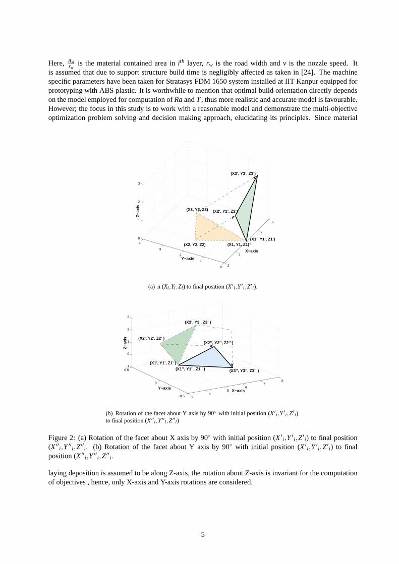
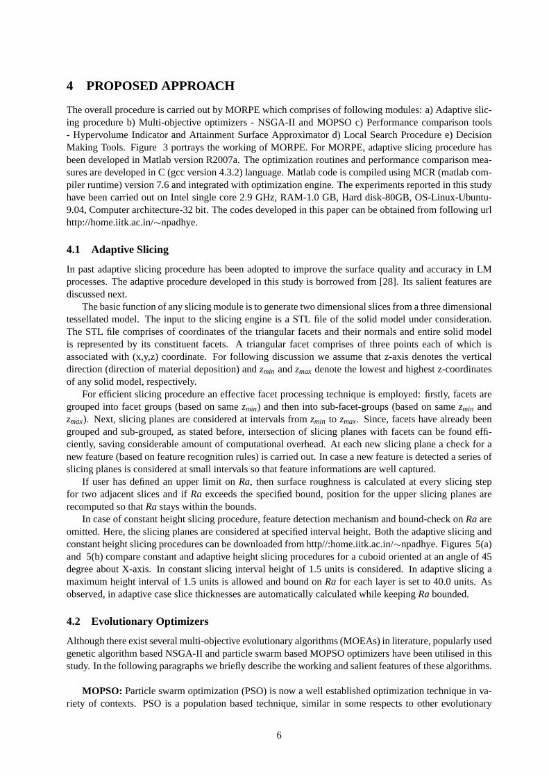
The problem variables areθx andθy representing the rotations from an initial configuration about somereference XYZ Cartesian coordinate system.

Figures 2(a) and 2(b) describe the rotation scheme stated here by considering rotation of a facet orplanar triangle (CAD model represented in form of facets can be rotated by rotation of all facets).

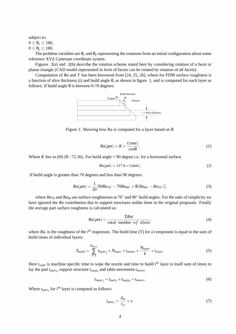
Computation ofRaandT has been borrowed from [24, 25, 26], where for FDM surface roughness isa function of slice thickness (t) and build angleθ, as shown in figure 1, and is computed for each layer asfollows: If build angleθ is between 0-70 degrees:

t = Slice thickness

θ

Build direction

NormalTangent

Figure 1: Showing how Ra is computed for a layer based onθ.

Ra(µm) = K×t(mm)

cosθ, (1)

WhereK lies in (69.28 - 72.36). For build angle = 90 degree i.e. for a horizontal surface

Ra(µm) = 117.6× t(mm), (2)

If build angle is greater than 70 degrees and less than 90 degrees:

Ra(µm) =120

[90Ra70◦ −70Ra90◦ +θ(Ra90◦ −Ra70◦)], (3)

whereRa70 andRa90 are surface roughnesses at 70◦ and 90◦ build angles. For the sake of simplicity wehave ignored theRacontribution due to support structures unlike done in the original proposals. Finallythe average part surface roughness is calculated as:

Ra(µm) =ΣRai

total number o f slices, (4)

whereRai is the roughness of theith trapezium. The build time (T) for a component is equal to the sum ofbuild times of individual layers.

Tbuild =Nlayer

∑i=1

tlayeri +Nlayer× tzmove+Nlayer

k× twipe, (5)

Heretwipe is machine specific time to wipe the nozzle and time to buildith layer is itself sum of times tolay the parttparti , support structuretsuppi and table movementtmovei .

tlayeri = tparti + tsuppi + tmovei , (6)

Wheretparti for ith layer is computed as follows:

tparti =Asi

rw×v. (7)

4

Here, Asirw

is the material contained area inith layer, rw is the road width andv is the nozzle speed. Itis assumed that due to support structure build time is negligibly affected as taken in [24]. The machinespecific parameters have been taken for Stratasys FDM 1650 system installed at IIT Kanpur equipped forprototyping with ABS plastic. It is worthwhile to mention that optimal build orientation directly dependson the model employed for computation ofRaandT, thus more realistic and accurate model is favourable.However; the focus in this study is to work with a reasonable model and demonstrate the multi-objectiveoptimization problem solving and decision making approach, elucidating its principles. Since material

2

3

4

5

6

0

1

2

3

4

0

1

2

3

X−axis

Y−axis

Z−a

xis

(X1, Y1, Z1)(X1’, Y1’, Z1’)

(X2, Y2, Z2)

(X3, Y3, Z3)

(X3’, Y3’, Z3’)

(X2’, Y2’, Z2’)

(a) n (Xi ,Yi ,Zi) to final position (X′i ,Y′

i ,Z′i).

34

56

78

−0.5

0

0.5−1

0

1

2

3

X−axisY−axis

Z−a

xis

(X1’, Y1’, Z1’ )

(X2’, Y2’, Z2’ )

(X1’’, Y1’’, Z1’’ ) (X3’’, Y3’’, Z3’’ )

(X2’’, Y2’’, Z2’’ )

(X3’, Y3’, Z3’ )

(b) Rotation of the facet about Y axis by 90◦ with initial position (X′i ,Y′

i ,Z′i)

to final position (X′′i ,Y′′

i ,Z′′i)

Figure 2: (a) Rotation of the facet about X axis by 90◦ with initial position (X′i ,Y′

i ,Z′i) to final position

(X′′i ,Y′′

i ,Z′′i . (b) Rotation of the facet about Y axis by 90◦ with initial position (X′

i ,Y′i ,Z′

i) to finalposition (X′′

i ,Y′′i ,Z′′

i .

laying deposition is assumed to be along Z-axis, the rotation about Z-axis is invariant for the computationof objectives , hence, only X-axis and Y-axis rotations are considered.

5

4 PROPOSED APPROACH

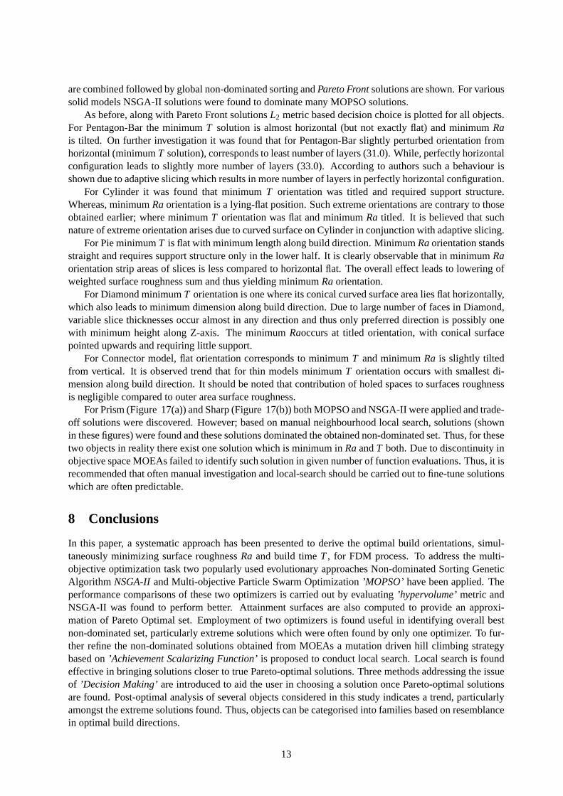
The overall procedure is carried out by MORPE which comprises of following modules: a) Adaptive slic-ing procedure b) Multi-objective optimizers - NSGA-II and MOPSO c) Performance comparison tools- Hypervolume Indicator and Attainment Surface Approximator d) Local Search Procedure e) DecisionMaking Tools. Figure 3 portrays the working of MORPE. For MORPE, adaptive slicing procedure hasbeen developed in Matlab version R2007a. The optimization routines and performance comparison mea-sures are developed in C (gcc version 4.3.2) language. Matlab code is compiled using MCR (matlab com-piler runtime) version 7.6 and integrated with optimization engine. The experimentsreported in this studyhave been carried out on Intel single core 2.9 GHz, RAM-1.0 GB, Hard disk-80GB, OS-Linux-Ubuntu-9.04, Computer architecture-32 bit. The codes developed in this paper canbe obtained from following urlhttp://home.iitk.ac.in/∼npadhye.

4.1 Adaptive Slicing

In past adaptive slicing procedure has been adopted to improve the surface quality and accuracy in LMprocesses. The adaptive procedure developed in this study is borrowed from [28]. Its salient features arediscussed next.

The basic function of any slicing module is to generate two dimensional slices from a three dimensionaltessellated model. The input to the slicing engine is a STL file of the solid model under consideration.The STL file comprises of coordinates of the triangular facets and their normals and entire solid modelis represented by its constituent facets. A triangular facet comprises of three points each of which isassociated with (x,y,z) coordinate. For following discussion we assume thatz-axis denotes the verticaldirection (direction of material deposition) andzmin andzmax denote the lowest and highest z-coordinatesof any solid model, respectively.

For efficient slicing procedure an effective facet processing technique is employed: firstly, facets aregrouped into facet groups (based on samezmin) and then into sub-facet-groups (based on samezmin andzmax). Next, slicing planes are considered at intervals fromzmin to zmax. Since, facets have already beengrouped and sub-grouped, as stated before, intersection of slicing planes with facets can be found effi-ciently, saving considerable amount of computational overhead. At eachnew slicing plane a check for anew feature (based on feature recognition rules) is carried out. In case a new feature is detected a series ofslicing planes is considered at small intervals so that feature informations are well captured.

If user has defined an upper limit onRa, then surface roughness is calculated at every slicing stepfor two adjacent slices and ifRa exceeds the specified bound, position for the upper slicing planes arerecomputed so thatRastays within the bounds.

In case of constant height slicing procedure, feature detection mechanism and bound-check onRaareomitted. Here, the slicing planes are considered at specified interval height. Both the adaptive slicing andconstant height slicing procedures can be downloaded from http//:home.iitk.ac.in/∼npadhye. Figures 5(a)and 5(b) compare constant and adaptive height slicing procedures for a cuboid oriented at an angle of 45degree about X-axis. In constant slicing interval height of 1.5 units is considered. In adaptive slicing amaximum height interval of 1.5 units is allowed and bound onRa for each layer is set to 40.0 units. Asobserved, in adaptive case slice thicknesses are automatically calculated while keepingRabounded.

4.2 Evolutionary Optimizers

Although there exist several multi-objective evolutionary algorithms (MOEAs) in literature, popularly usedgenetic algorithm based NSGA-II and particle swarm based MOPSO optimizers have been utilised in thisstudy. In the following paragraphs we briefly describe the working and salient features of these algorithms.

MOPSO: Particle swarm optimization (PSO) is now a well established optimization technique inva-riety of contexts. PSO is a population based technique, similar in some respectsto other evolutionary

6

algorithms, except that potential solutions (particles) move rather than evolve through the search space.PSO consists of several candidate solutions called particles each of whichhas a position and velocity, andexperiences linear spring-like attractions towards two attractors:

1) the best position attained by that particle so far (particle attractor or personal best (pbest);

2) the best of the particle attractors in a certain neighbourhood (neighbourhood attractor or global bestglobal best).

More recently, PSO has successfully been extended to multi-objective optimization problems and suchmethods are called Multi-objective Particle Swarm Optimization (MOPSO). Its simpleimplementation,population based approach, success in handling continuous search spaces and notions of individual posi-tion and velocity are major reasons for its popularity. PSO works with a population of individuals each ofwhich is subjected to movement in direction of‘Pbest’ - position corresponding to best fitness attained byan individual and a‘Gbest’ - position of best fitness individual in the entire population. In each generationor cycle (‘t’), every individual is associated with a position vector (φt) and a velocity vector ( ¯vt). The sizeof these vectors is equal to the size of the vectorφt . The position and velocity of each individual is updatedaccording to following equations:

vt = wvt +c1r1 · (pg,t − φt)+c2r2 · ( ¯GBestt − φt)

¯φt+1 = vt + φt

¯φt+1 = φt + δ

Above are position and velocity update equations. The termw is known as inertia weight and,c1

and c2 are known as learning factors. In our procedurew has been chosen as 0.5,c1 and c2 are bothtaken to be 1.0. Once velocities and positions have been updated, a randomperturbation, donated byδ, isadded to an individual’s position based on some probability. This is known as‘turbulence factor’ and isanalogous to ”mutation” employed in Genetic Algorithms. Goal of ”turbulence” isto preserve diversity inthe population.

The MOPSO utilised in this study has been borrowed from [22, 23]. At the start of optimization, forall N particles positions (φ) are initialised randomly and velocities (v) are set to zero. At the onset pbestfor each particle is assigned as the the particle itself. The current MOPSO maintains an external archive ofnon-dominated solutions of the population which is updated after every generation. This global archive isempty in the beginning and can store a maximum number of non-dominated solutionswhich is specified atthe start. In case the number of non-dominated solutions exceed the maximum size of the archive, in anygeneration, clustering is invoked to restore the archive size. For each particle in the population a personalarchive, also calledpbest archiveis maintained. The pbest archive contains the most recent non-dominatedpositions that particle has encountered while searching the space. Such additional archiving scheme forthe particles is often found to be extremely effective.

In every generation, each particle is assigned two guides pbest and gbest from its pbest archive andswarms global archive. The way in which these guides are allocated has agreat impact on algorithmsperformance. Several methods for guide selections exist. In this study, ‘NWtd.’ and ‘Dom.’ methods forpersonal best selection and global best selection have been chosen .For more details on guide selection inMOPSO reader is referred to [21, 23]. Maximum number of generations isset as the termination criterion.

NSGA-II: Elitist Non-Dominated Sorting Genetic Algorithm (NSGA-II) is one of the most popularlyused GA for multi-objective optimization. Several salient features like elite preservation and explicit di-versity preserving mechanisms ensure its good convergence and diversity. Brief description of NSGA-II

7

procedure is described here, for further details reader is referredto [8, 9]: Offspring population (size N)is created using parent population (size N) by usual genetic operators -selection, crossover and mutation.The created child population is combined with parent population, to form combined population of size 2N,and then a non-dominated sorting is carried out to classify the entire population into several non-dominatedfronts. The new population (size N) is then filled by the members of combined population belonging to dif-ferent non-dominated levels or starting from first level. Since all members of combined population cannotbe accommodated in new population - several non-dominated fronts have to discarded. Since all membersof last front entering the new population may not be accommodated, only fewmembers (correspondingto number of available slots) are selected from the last front based on the crowding distance technique.Binary tournament selection, SBX, and polynomial mutation operators are used for NSGA-II.

4.3 Performance Comparisons

Due to stochastic nature of evolutionary approaches, it is difficult to conclude anything about performancefrom just one simulation run. To eliminate the random effects and gather results of statistical significance,we perform multiple (11) runs of both the algorithms corresponding to different initial seeds. Two per-formance measures commonly used in EA literature have been employed in this study are described asfollows:

Attainment Surfaces: Multiple runs, corresponding to different initial seeds, of an evolutionary algo-rithm usually result in multiple non-dominated set. Thus, to deduce overall performance an approximationof best non-dominated set, also referred to as 1st (0%) attainment surface, is computed from available non-dominated sets. Since non-dominated can be visualised easily in two and three dimensions, such a methodprovides good insight into algorithms performance. The computation of attainment surfaces is done byusing attainment surface package described in [15].

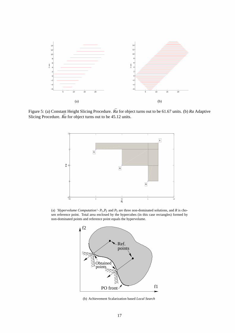
Hypervolume indicator: Hypervolume is a measurement which takes into account the diversity as wellas the convergence of the solutions [36]. Hypervolume represents the sum of the areas enclosed withinthe hypercubes formed by the points on the non-dominated front and a chosen reference point. For min-imisation type problems a higher value of hypervolume is desirable, as it is indicative of better spread andconvergence of solutions. Figure 6(a) illustrates the hypervolume computation for a set of non-dominatedpoints with respect to a reference point ’R’. It should be noted that contribution to hypervolume is onlymade by points which are dominated by the reference point. All points not dominated by the referencepoint have zero contribution to the hypervolume. In this study we have computed average hypervolumecurves over several generations for study and comparisons purposes. Although, hypervolume computationis dependent on choice of reference point, yet it is regarded as a good measure and can be employed forhigher number of objectives as well.

4.4 Local Search Method

Typically for any practical multi-objective optimization problem location of true Pareto-optimal solutionsis unknown. Although, MOEAs provide a good means to reach approximate or close to Pareto-optimalsolutions, often further improvement on obtained solutions is possible by conductinglocal search. Localsearch usually considers an already found non-dominated solution and tries to improve it by utilising aconstruction of single objective function.

In this study we construct an achievement scalarizing function (ASF), a single objective function, andconsider its minimization. Following describes ASF scheme:

Consider such a starting pointy (having objective vectorf(y) andz=f(y)), then ASF = :

8

minx∈ S⊂ R

n

Mmaxi=1

fi(x)−zi

f maxi − f min

i+ ρ

M∑j=1

f j (x)−zj

f maxj − f min

j

Wherez=f(y) is usually referred to as a reference point for local search, andf maxi and f min

i are mini-mum objective values of the ’best non-dominated’ set. By this minimization,ASFs solutions are projectedon the Pareto-front and convergence can be guaranteed.

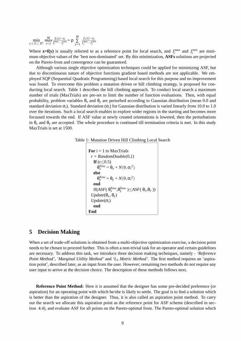
Although various single objective optimization techniques could be applied forminimizing ASF, butdue to discontinuous nature of objective functions gradient based methods are not applicable. We em-ployed SQP (Sequential Quadratic Programming) based local search forthis purpose and no improvementwas found. To overcome this problem a mutation driven or hill climbing strategy, is proposed for con-ducting local search. Table 1 describes the hill climbing approach. To conduct local search a maximumnumber of trials (MaxTrials) are pre-set to limit the number of function evaluations. Then, with equalprobability, problem variablesθx andθy are perturbed according to Gaussian distribution (mean 0.0 andstandard deviationσi). Standard deviation (σi) for Gaussian distribution is varied linearly from 10.0 to 1.0over the iterations. Such a local search enables to explore wider regionsin the starting and becomes morefocussed towards the end. If ASF value at newly created orientations is lowered, then the perturbationsin θx andθy are accepted. The whole procedure is continued till termination criteria is met. In this studyMaxTrials is set at 1500.

Table 1: Mutation Driven Hill Climbing Local Search

For i = 1 to MaxTrialsr = RandomDouble(0,1)

If (r≤0.5)θNew

x = θx + N(0,σi2)

elseθNew

y = θy + N(0,σi2)

endIf(ASF( θNew

x ,θNewy )≤ASF( θx,θy ))

Update(θx, θy)Update(σi)

endEnd

5 Decision Making

When a set of trade-off solutions is obtained from a multi-objective optimizationexercise, a decision pointneeds to be chosen to proceed further. This is often a non-trivial task for an operator and certain guidelinesare necessary. To address this task, we introduce three decision makingtechniques, namely -‘ReferencePoint Method’, ‘Marginal Utility Method’ and‘L2 Metric Method’. The first method requires an ’aspira-tion point’, described later, as an input from the user. However; remaining two methods do not require anyuser input to arrive at the decision choice. The description of these methods follows next.

Reference Point Method: Here it is assumed that the designer has some pre-decided preference (oraspiration) for an operating point with which he/she is likely to settle. The goalis to find a solution whichis better than the aspiration of the designer. Thus, it is also called an aspiration point method. To carryout the search we allocate this aspiration point as the reference point forASF scheme (described in sec-tion 4.4), and evaluate ASF for all points on the Pareto-optimal front. The Pareto-optimal solution which

9

corresponds to lowest ASF value, with respect to reference point, is selected. For illustration purposes,following three aspiration points are considered in this study.

Asp1= (Ramin+Ramax2 ,Tmin+Tmax

2 ),

Asp2= (Ramin+Ramax2 , Tmax),

Asp3= (Ramax,Tmin+Tmax

2 )

The corresponding decision choices obtained on the Pareto-front will be indicated asP1, P2 andP3. Asp1,for example, implies that user is willing to accept an available point in proximity of the mean of best andworst obtained (Ra, T) values. In case of convex Pareto-optimal decision choice dominates the aspirationpoint, whereas in case of concave set decision choice gets dominated by the aspiration point.

Marginal Utility Method: This approach also does not require any prior information from the userandsearches for a Pareto-optimal solution which shows least affinity towardsany of its neighbours in objec-tive space. To compute the affinity towards the neighbourhood, considerthree non-dominated pointsP1, P0

andP2, s.t. (Ra1≤Ra0≤Ra2) and (T1≥T0≥T2) and we are interested in evaluating the affinity at the middlepoint P0. P1 andP2 lie in the neighbourhood ofP0 and are selected as follows: considerk points,P0,m m= 1 tok, nearest toP0, with Ra0,m ≤ Ra0. Then centroid of allP0,ms is computed and a point out ofP0,ms,which is closest to the centroid, is selected asP1. For selectingP2, same exercise is repeated, but this timeconsidering points s.t.Ra0,ms are greater thanRa0.

OnceP1 andP2 are computed forP0, affinity function(AF), is calculated as :

AFP0=max(W1,W2); W1=RaP0−RaP1

TP1−TP0and W2=

RaP2−RaP0TP0−TP2

.

For each point in the non-dominated set, except fork extreme points at both ends,AF is computed and thesolution with minimumAF is assigned as decision choice. This solution is argued to posses least affinitytowards any of its neighbours. In this study value of k is taken equal to 6. The value ofk decides theresolution of the proximity in which we are interested to compute the affinity function. Decision pointpoint by this method is usually a ‘knee point’.‘Knee points’ are often of great practical importance as theydenote a coordinate on Pareto-front where increase (decrease) in one objective is very large compared todecrease (or increase ) in other objective.

L2-metric: This is a straight-forward method to select one solution out of many non-dominated solu-tions without requiring any information from user. Firstly, each objective isnormalised in [0.0, 1.0]. Thenan ’ideal point’ is constructed, which is origin in case of normalised space, and taken as thereferencepoint. Euclidean distance (L2) of each point in the non-dominated set is calculated from the referencepoint and the solution with smallest Euclidean distance is finally selected.

6 Experiments

In this section a series of simulations are performed on various solid models to demonstrate the workingof MORPE. The major goals of this study are:

1. Compare the performances of MOPSO and NSGA-II by computing hypervolume over generations,and draw conclusions on their convergence and diversity preservation characteristics.

2. Approximate the Pareto-optimal set by computing 1st (0%) attainment surface from 11 runs of each

10

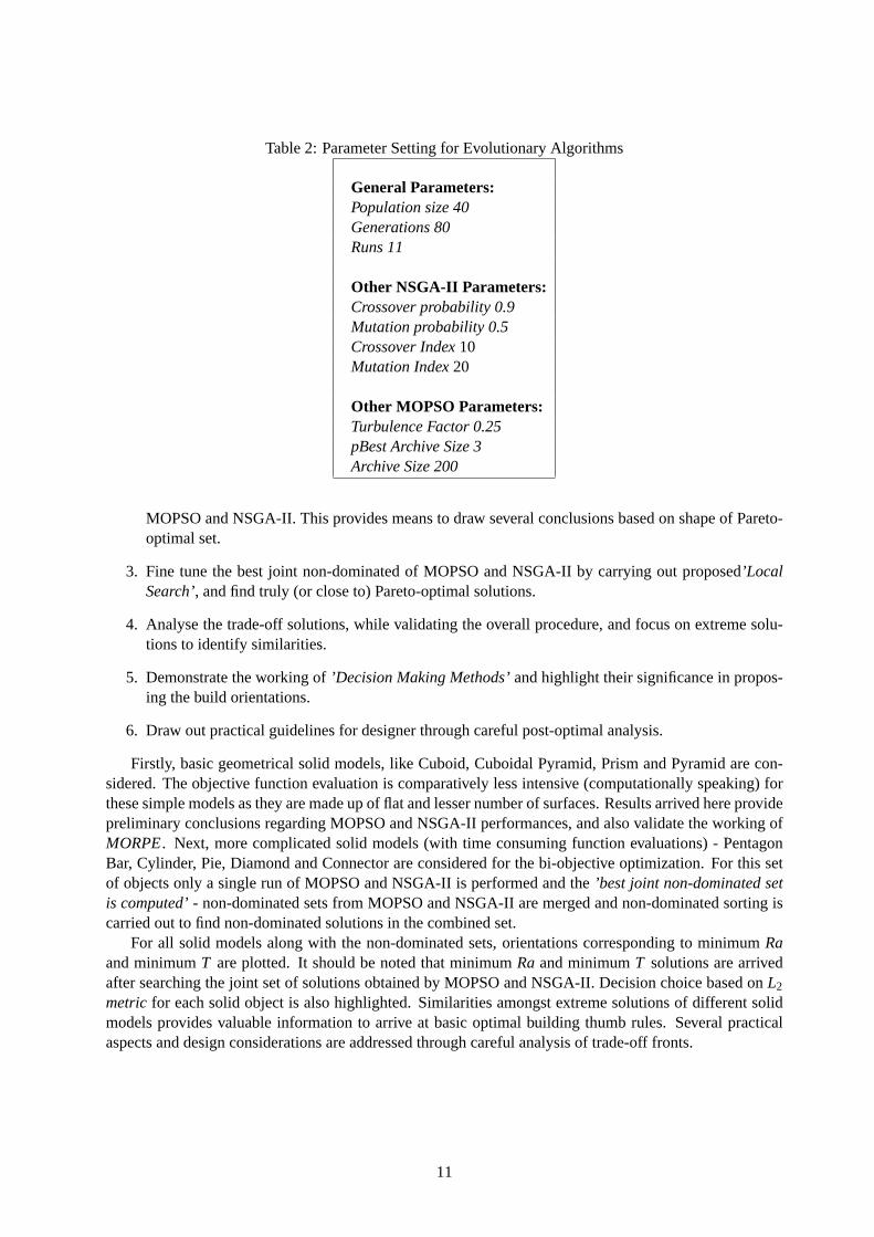
Table 2: Parameter Setting for Evolutionary Algorithms

General Parameters:Population size 40Generations 80Runs 11

Other NSGA-II Parameters:Crossover probability 0.9Mutation probability 0.5Crossover Index10Mutation Index20

Other MOPSO Parameters:Turbulence Factor 0.25pBest Archive Size 3Archive Size 200

MOPSO and NSGA-II. This provides means to draw several conclusions based on shape of Pareto-optimal set.

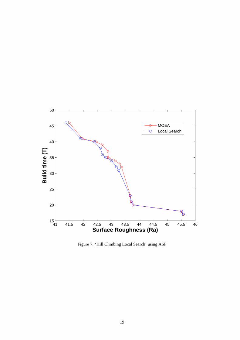
3. Fine tune the best joint non-dominated of MOPSO and NSGA-II by carrying out proposed’LocalSearch’, and find truly (or close to) Pareto-optimal solutions.

4. Analyse the trade-off solutions, while validating the overall procedure, and focus on extreme solu-tions to identify similarities.

5. Demonstrate the working of’Decision Making Methods’and highlight their significance in propos-ing the build orientations.

6. Draw out practical guidelines for designer through careful post-optimal analysis.

Firstly, basic geometrical solid models, like Cuboid, Cuboidal Pyramid, Prism and Pyramid are con-sidered. The objective function evaluation is comparatively less intensive(computationally speaking) forthese simple models as they are made up of flat and lesser number of surfaces. Results arrived here providepreliminary conclusions regarding MOPSO and NSGA-II performances,and also validate the working ofMORPE. Next, more complicated solid models (with time consuming function evaluations) - PentagonBar, Cylinder, Pie, Diamond and Connector are considered for the bi-objective optimization. For this setof objects only a single run of MOPSO and NSGA-II is performed and the’best joint non-dominated setis computed’- non-dominated sets from MOPSO and NSGA-II are merged and non-dominated sorting iscarried out to find non-dominated solutions in the combined set.

For all solid models along with the non-dominated sets, orientations corresponding to minimumRaand minimumT are plotted. It should be noted that minimumRa and minimumT solutions are arrivedafter searching the joint set of solutions obtained by MOPSO and NSGA-II. Decision choice based onL2

metric for each solid object is also highlighted. Similarities amongst extreme solutions ofdifferent solidmodels provides valuable information to arrive at basic optimal building thumb rules. Several practicalaspects and design considerations are addressed through careful analysis of trade-off fronts.

11

7 Results and Discussions

In general, it is difficult to predict an optimal build direction for any solid model.Major difficulty arisesdue to non-linear nature and non-differentiable expressions for surface roughness. This is the major reasonfor using an optimization procedure. For the minimum time orientations least numberof layers are desired.Since layer thicknesses vary according to the adaptive slicing procedure described earlier, an orientationwith minimum length in build direction may contain more layers as compared to some otherdirection.Hence the total number of slices depends on slice thicknesses which in turn solely depends on the localgeometry of the solid model.

An orientation in which faces are inclined with respect to vertical requires asupport structure andis likely to result in higher surface roughness. However, one should note that due to adaptive slicingprocedure local surface roughness is limited and appearance of support structure is counteracted by thinnerslices, thus increasing the number of slices. The thinner slices are also associated with smaller strip areas,and since local roughness is weighted with the strip areas the overall surface roughness tends to decrease.For an optimal solution these two opposing factors are balanced. This also explains why a trade-off existsbetween the build time and surface roughness.

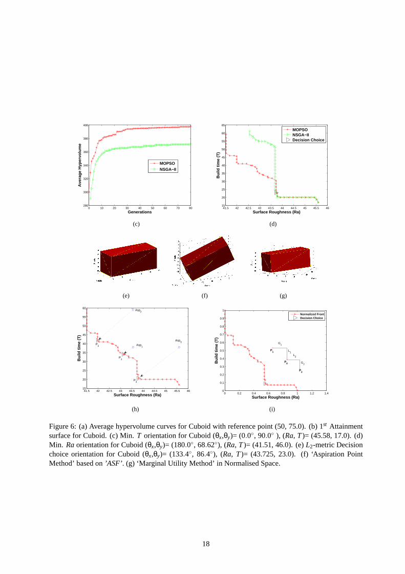
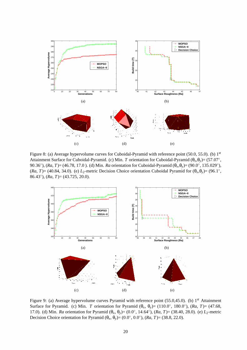
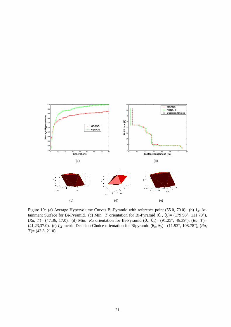
Figures 6, 8, 9 and 10 show the hypervolume curves, 1st (0 %) attainment surfaces of MOPSO andNSGA-II from 11 runs, extreme solutions corresponding to minimumT and minimumRaorientations andL2 metric based decision choice. For each shown orientation the decision variables and (Ra, T) are stated.

Based on hypervolume curves and attainment surfaces MOPSO performsbetter than NSGA-II, forCuboid. In all hypervolume curves MOPSO shows fatser convergencebehaviour in initial few generations,as hypervolume rises rapidly, but eventually settles at values lesser than NSGA-II hypervolume values,except for Cuboid where MOPSO performs better than NSGA-II both in terms of hypervolume and 1st

(0%) attainment surfaces. Hypervolume trends of MOPSO indicatepremature convergence- a well knowndrawback in particle swarm optimization (PSO). According to the authors pre-mature convergence ofMOPSO, in this case, highlights the absence of potential global guides due todiscontinuities present in theobjective space. Presence of discontinuity slows the march towards the true Pareto-optimal solutions. ForCuboidal Pyramid, Pyramid and Bipyramid NSGA-II clearly performs better as indicated by hypervolumecurves. From attainment surfaces it can be observed that major regionsof 1st (0%) attainment surface ofMOPSO are dominated by NSGA-II attainment surface. However; extreme solutions corresponding tominimumT or minimumRawere sometimes found better by MOPSO.

For these four objects the minimum time orientation occurs when minimum dimension occurs along Z-direction (build orientation). Planar surfaces of in these solid objects result in flat orientations for minimumT. It can be argued that particularly in absence of curved surfaces slicing occurs with uniform thicknessand minimum length dimension leads to least number of slices. MinimumRa orientation is not easy toguess and occurs at titled configuration, requiring support structure.

For Cuboid, decision choice based on’Reference Point Method’and’Marginal Utility’ are also shownin Figures 6(h) and 6(i), respectively. Three solutions are found by’Aspiration Method’correspondingto three aspiration points.’Marginal Utility Method’ discovers theknee point, the point with least affinity.At any such’knee point’there is a large trade-off in one objective for marginal trade-off in otherobjective.According to Figure 6(i) at theknee pointdecrease inRa is accompanied by a large increase inT. Thus,user would ideally like to work at the marked knee position. For all four solid modelsL2 metric basedconfiguration is also shown and lies spatially in between the two extreme configuration.

Overall it can be concluded that NSGA-II shows an acceptable better performance and application ofanother evolutionary optimizer MOPSO may be advantageous in providing somebetter solutions. The factthat attainment surfaces of MOPSO and NSGA-II have similar spread and distribution further builds ourconfidence on obtained solutions and their proximity to true Pareto optimal solutions.

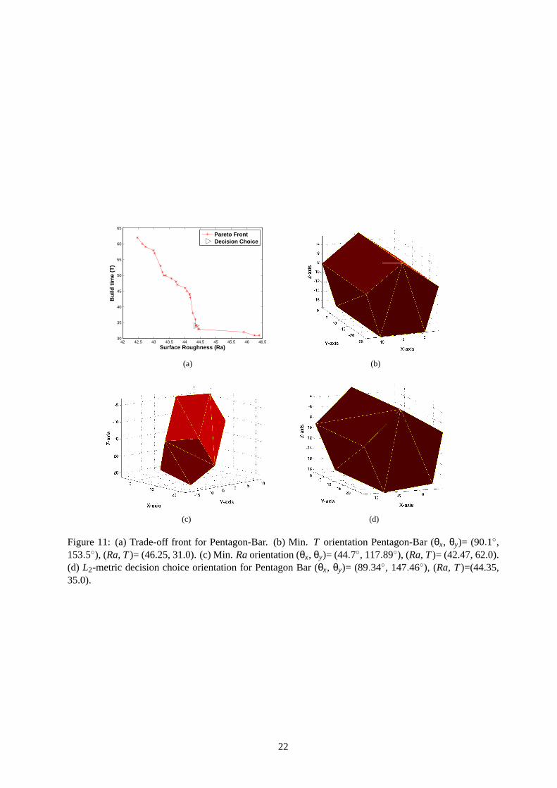
Next, we consider more complicated solid models - Pentagon-Bar, Cylinder, Pie shape, Diamond andConnector in Figures 11-17. Since function evaluations for these solid models is computationally intensive,a single run of MOPSO and NSGA-II is considered. Non-dominated sets from NSGA-II and MOPSO runs

12

are combined followed by global non-dominated sorting andPareto Frontsolutions are shown. For varioussolid models NSGA-II solutions were found to dominate many MOPSO solutions.

As before, along with Pareto Front solutionsL2 metric based decision choice is plotted for all objects.For Pentagon-Bar the minimumT solution is almost horizontal (but not exactly flat) and minimumRais tilted. On further investigation it was found that for Pentagon-Bar slightly perturbed orientation fromhorizontal (minimumT solution), corresponds to least number of layers (31.0). While, perfectly horizontalconfiguration leads to slightly more number of layers (33.0). According to authors such a behaviour isshown due to adaptive slicing which results in more number of layers in perfectly horizontal configuration.

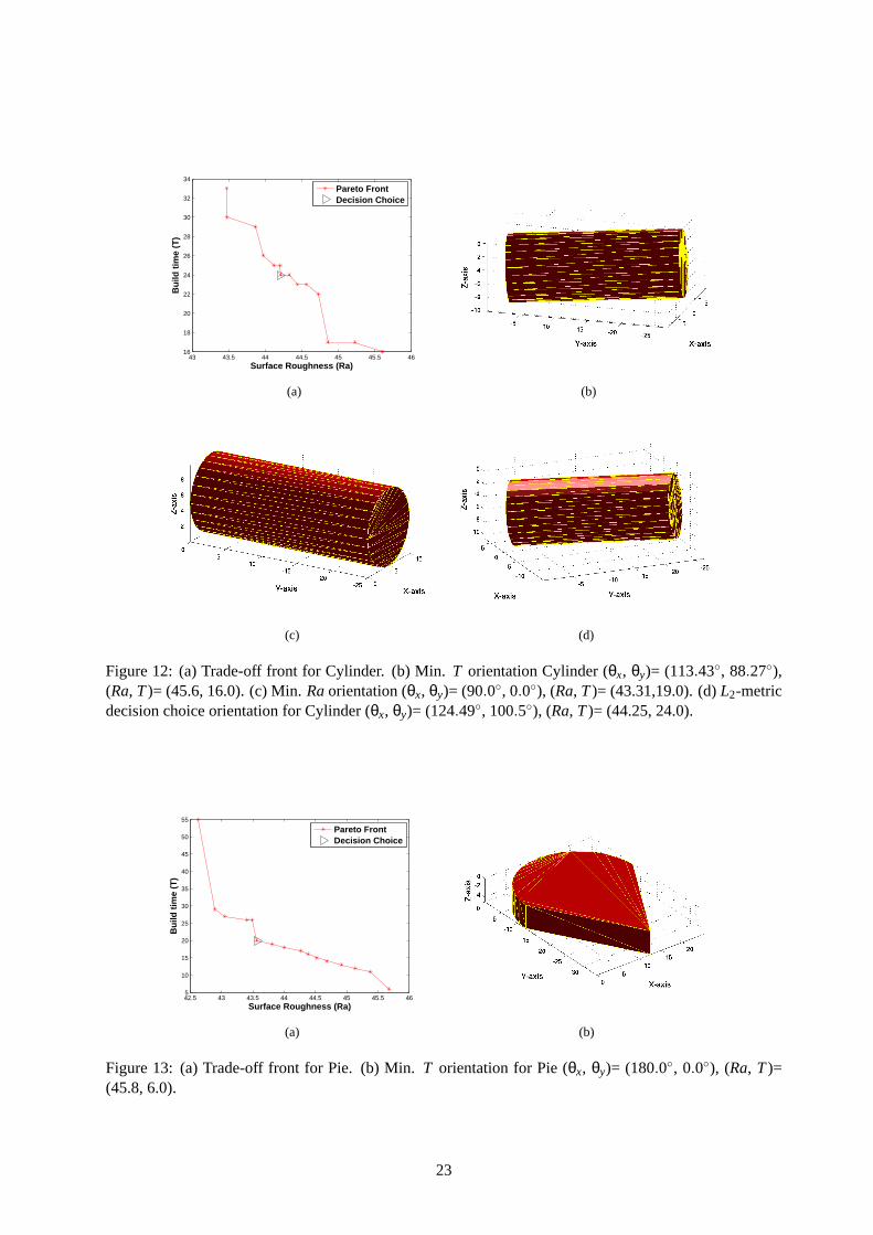
For Cylinder it was found that minimumT orientation was titled and required support structure.Whereas, minimumRaorientation is a lying-flat position. Such extreme orientations are contrary to thoseobtained earlier; where minimumT orientation was flat and minimumRa titled. It is believed that suchnature of extreme orientation arises due to curved surface on Cylinder in conjunction with adaptive slicing.

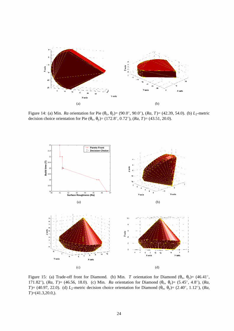
For Pie minimumT is flat with minimum length along build direction. MinimumRaorientation standsstraight and requires support structure only in the lower half. It is clearly observable that in minimumRaorientation strip areas of slices is less compared to horizontal flat. The overall effect leads to lowering ofweighted surface roughness sum and thus yielding minimumRaorientation.

For Diamond minimumT orientation is one where its conical curved surface area lies flat horizontally,which also leads to minimum dimension along build direction. Due to large number of faces in Diamond,variable slice thicknesses occur almost in any direction and thus only preferred direction is possibly onewith minimum height along Z-axis. The minimumRaoccurs at titled orientation, with conical surfacepointed upwards and requiring little support.

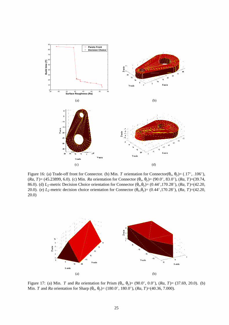
For Connector model, flat orientation corresponds to minimumT and minimumRa is slightly tiltedfrom vertical. It is observed trend that for thin models minimumT orientation occurs with smallest di-mension along build direction. It should be noted that contribution of holed spaces to surfaces roughnessis negligible compared to outer area surface roughness.

For Prism (Figure 17(a)) and Sharp (Figure 17(b)) both MOPSO and NSGA-II were applied and trade-off solutions were discovered. However; based on manual neighbourhood local search, solutions (shownin these figures) were found and these solutions dominated the obtained non-dominated set. Thus, for thesetwo objects in reality there exist one solution which is minimum inRaandT both. Due to discontinuity inobjective space MOEAs failed to identify such solution in given number of function evaluations. Thus, it isrecommended that often manual investigation and local-search should be carried out to fine-tune solutionswhich are often predictable.

8 Conclusions

In this paper, a systematic approach has been presented to derive the optimal build orientations, simul-taneously minimizing surface roughnessRa and build timeT, for FDM process. To address the multi-objective optimization task two popularly used evolutionary approaches Non-dominated Sorting GeneticAlgorithm NSGA-IIand Multi-objective Particle Swarm Optimization’MOPSO’ have been applied. Theperformance comparisons of these two optimizers is carried out by evaluating’hypervolume’metric andNSGA-II was found to perform better. Attainment surfaces are also computed to provide an approxi-mation of Pareto Optimal set. Employment of two optimizers is found useful in identifying overall bestnon-dominated set, particularly extreme solutions which were often found byonly one optimizer. To fur-ther refine the non-dominated solutions obtained from MOEAs a mutation driven hill climbing strategybased on’Achievement Scalarizing Function’is proposed to conduct local search. Local search is foundeffective in bringing solutions closer to true Pareto-optimal solutions. Three methods addressing the issueof ’Decision Making’are introduced to aid the user in choosing a solution once Pareto-optimal solutionsare found. Post-optimal analysis of several objects considered in this study indicates a trend, particularlyamongst the extreme solutions found. Thus, objects can be categorised intofamilies based on resemblancein optimal build directions.

13

9 Acknowledgements

First author sincerely thanks Dr. N.V. Reddy and Dr. P.M. Pandey for introducing the problem and showingconsistent support.

14

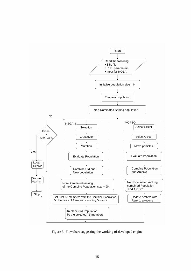
Figure 3: Flowchart suggesting the working of developed engine

15

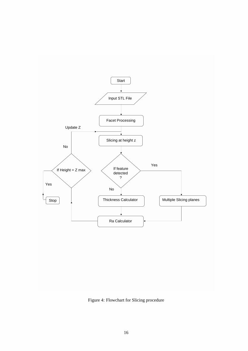
Figure 4: Flowchart for Slicing procedure

16

5 10 15 20

−6

−4

−2

0

2

4

6

8

10

12

14

Z−

axis

(a)

5 10 15 20

−6

−4

−2

0

2

4

6

8

10

12

14

Z−

axis

(b)

Figure 5: (a) Constant Height Slicing Procedure.Rafor object turns out to be 61.67 units. (b)RaAdaptiveSlicing Procedure.Rafor object turns out to be 45.12 units.

−0.5 0 0.5 1 1.5−0.5

0

0.5

1

1.5

F1

F2

P1

P2

P3

R

(a) ’Hypervolume Computation’- P1,P2 andP3 are three non-dominated solutions, andR is cho-sen reference point. Total area enclosed by the hypercubes (in this case rectangles) formed bynon-dominated points and reference point equals the hypervolume.

points

f1

f2

pointsRef.

Obtained

PO front

(b) Achievement Scalarization basedLocal Search

17

0 10 20 30 40 50 60 70 80280

300

320

340

360

380

400

Generations

Ave

rage

Hyp

ervo

lum

e

MOPSONSGA−II

(c)

41.5 42 42.5 43 43.5 44 44.5 45 45.5 4615

20

25

30

35

40

45

50

55

60

65

Surface Roughness (Ra)B

uild

tim

e (T

)

MOPSONSGA−IIDecision Choice

(d)

(e) (f) (g)

41.5 42 42.5 43 43.5 44 44.5 45 45.5 4615

20

25

30

35

40

45

50

55

60

Surface Roughness (Ra)

Bui

ld ti

me

(T)

Asp2

Asp3

Asp1

P1

P2

P3

(h)

0 0.2 0.4 0.6 0.8 1 1.2 1.40

0.1

0.2

0.3

0.4

0.5

0.6

0.7

0.8

0.9

1

Surface Roughness (Ra)

Bui

ld ti

me

(T)

Normalized FrontDecision Choice

P1

G1

G2

L1

L2

P0

P2

(i)

Figure 6: (a) Average hypervolume curves for Cuboid with referencepoint (50, 75.0). (b) 1st Attainmentsurface for Cuboid. (c) Min.T orientation for Cuboid (θx,θy)= (0.0◦, 90.0◦ ), (Ra, T)= (45.58, 17.0). (d)Min. Raorientation for Cuboid (θx,θy)= (180.0◦, 68.62◦), (Ra, T)= (41.51, 46.0). (e)L2-metric Decisionchoice orientation for Cuboid (θx,θy)= (133.4◦, 86.4◦), (Ra, T)= (43.725, 23.0). (f) ‘Aspiration PointMethod’ based on’ASF’. (g) ‘Marginal Utility Method’ in Normalised Space.

18

41 41.5 42 42.5 43 43.5 44 44.5 45 45.5 4615

20

25

30

35

40

45

50

Surface Roughness (Ra)

Bui

ld ti

me

(T)

MOEALocal Search

Figure 7: ‘Hill Climbing Local Search’ using ASF

19

0 10 20 30 40 50 60 70 80210

220

230

240

250

260

270

280

290

300

Generations

Ave

rage

Hyp

ervo

lum

e

MOPSONSGA−II

(a)

40 41 42 43 44 45 46 4715

20

25

30

35

40

Surface Roughness (Ra)

Bui

ld ti

me

(T)

MOPSONSGA−IIDecision Choice

(b)

(c) (d) (e)

Figure 8: (a) Average hypervolume curves for Cuboidal-Pyramid with reference point (50.0, 55.0). (b) 1st

Attainment Surface for Cuboidal-Pyramid. (c) Min.T orientation for Cuboidal-Pyramid (θx,θy)= (57.07◦,90.36◦), (Ra, T)= (46.78, 17.0 ). (d) Min.Raorientation for Cuboidal-Pyramid (θx,θy)= (90.0◦, 135.029◦),(Ra, T)= (40.84, 34.0). (e)L2-metric Decision Choice orientation Cuboidal Pyramid for (θx,θy)= (96.1◦,86.43◦), (Ra, T)= (43.725, 20.0).

0 10 20 30 40 50 60 70 80320

340

360

380

400

420

440

Generations

Ave

rage

Hyp

ervo

lum

e

MOPSONSGA−II

(a)

38 39 40 41 42 43 44 45 46 47 4816

18

20

22

24

26

28

30

32

Surface Roughness (Ra)

Bui

ld ti

me

(T)

MOPSONSGA−IIDecision Choice

(b)

(c) (d) (e)

Figure 9: (a) Average hypervolume curves Pyramid with reference point (55.0,45.0). (b) 1st AttainmentSurface for Pyramid. (c) Min.T orientation for Pyramid (θx, θy)= (110.0◦, 180.0◦), (Ra, T)= (47.68,17.0). (d) Min.Raorientation for Pyramid (θx, θy)= (0.0◦, 14.64◦), (Ra, T)= (38.40, 28.0). (e)L2-metricDecision Choice orientation for Pyramid (θx, θy)= (0.0◦, 0.0◦), (Ra, T)= (38.8, 22.0).

20

0 10 20 30 40 50 60 70 80570

580

590

600

610

620

630

640

650

660

670

Generations

Ave

rage

Hyp

ervo

lum

e

MOPSONSGA−II

(a)

41 42 43 44 45 46 47 4815

20

25

30

35

40

45

50

55

Surface Roughness (Ra)

Bui

ld ti

me

(T)

MOPSONSGA−IIDecision Choice

(b)

(c) (d) (e)

Figure 10: (a) Average Hypervolume Curves Bi-Pyramid with referencepoint (55.0, 70.0). (b) 1st At-tainment Surface for Bi-Pyramid. (c) Min.T orientation for Bi-Pyramid (θx, θy)= (179.98◦, 111.79◦),(Ra, T)= (47.36, 17.0). (d) Min.Ra orientation for Bi-Pyramid (θx, θy)= (91.25◦, 46.39◦), (Ra, T)=(41.23,37.0). (e)L2-metric Decision Choice orientation for Bipyramid (θx, θy)= (11.93◦, 108.78◦), (Ra,T)= (43.8, 21.0).

21

42 42.5 43 43.5 44 44.5 45 45.5 46 46.530

35

40

45

50

55

60

65

Surface Roughness (Ra)

Bui

ld ti

me

(T)

Pareto FrontDecision Choice

(a) (b)

(c) (d)

Figure 11: (a) Trade-off front for Pentagon-Bar. (b) Min.T orientation Pentagon-Bar (θx, θy)= (90.1◦,153.5◦), (Ra, T)= (46.25, 31.0). (c) Min.Raorientation (θx, θy)= (44.7◦, 117.89◦), (Ra, T)= (42.47, 62.0).(d) L2-metric decision choice orientation for Pentagon Bar (θx, θy)= (89.34◦, 147.46◦), (Ra, T)=(44.35,35.0).

22

43 43.5 44 44.5 45 45.5 4616

18

20

22

24

26

28

30

32

34

Surface Roughness (Ra)

Bui

ld ti

me

(T)

Pareto FrontDecision Choice

(a) (b)

(c) (d)

Figure 12: (a) Trade-off front for Cylinder. (b) Min.T orientation Cylinder (θx, θy)= (113.43◦, 88.27◦),(Ra, T)= (45.6, 16.0). (c) Min.Raorientation (θx, θy)= (90.0◦, 0.0◦), (Ra, T)= (43.31,19.0). (d)L2-metricdecision choice orientation for Cylinder (θx, θy)= (124.49◦, 100.5◦), (Ra, T)= (44.25, 24.0).

42.5 43 43.5 44 44.5 45 45.5 465

10

15

20

25

30

35

40

45

50

55

Surface Roughness (Ra)

Bui

ld ti

me

(T)

Pareto FrontDecision Choice

(a) (b)

Figure 13: (a) Trade-off front for Pie. (b) Min.T orientation for Pie (θx, θy)= (180.0◦, 0.0◦), (Ra, T)=(45.8, 6.0).

23

(a) (b)

Figure 14: (a) Min.Raorientation for Pie (θx, θy)= (90.0◦, 90.0◦), (Ra, T)= (42.39, 54.0). (b)L2-metricdecision choice orientation for Pie (θx, θy)= (172.8◦, 0.72◦), (Ra, T)= (43.51, 20.0).

40 41 42 43 44 45 46 4718

18.5

19

19.5

20

20.5

21

21.5

22

Surface Roughness (Ra)

Bui

ld ti

me

(T)

Pareto FrontDecision Choice

(a) (b)

(c) (d)

Figure 15: (a) Trade-off front for Diamond. (b) Min.T orientation for Diamond (θx, θy)= (46.41◦,171.82◦), (Ra, T)= (46.56, 18.0). (c) Min. Ra orientation for Diamond (θx, θy)= (5.45◦, 4.8◦), (Ra,T)= (40.97, 22.0). (d)L2-metric decision choice orientation for Diamond (θx, θy)= (2.40◦, 1.12◦), (Ra,T)=(41.3,20.0,).

24

39 40 41 42 43 44 45 460

10

20

30

40

50

60

70

80

90

Surface Roughness (Ra)

Bui

ld ti

me

(T)

Pareto FrontDecision Choice

(a) (b)

(c) (d)

Figure 16: (a) Trade-off front for Connector. (b) Min.T orientation for Connector(θx, θy)= (.17◦, .106◦),(Ra, T)= (45.23899, 6.0). (c) Min.Raorientation for Connector (θx, θy)= (90.0◦, 83.0◦), (Ra, T)=(39.74,86.0). (d)L2-metric Decision Choice orientation for Connector (θx,θy)= (0.44◦,170.28◦), (Ra, T)=(42.20,20.0). (e)L2-metric decision choice orientation for Connector (θx,θy)= (0.44◦,170.28◦), (Ra, T)=(42.20,20.0)

(a) (b)

Figure 17: (a) Min.T andRa orientation for Prism (θx, θy)= (90.0◦, 0.0◦), (Ra, T)= (37.69, 20.0). (b)Min. T andRaorientation for Sharp (θx, θy)= (180.0◦, 180.0◦), (Ra, T)=(40.36, 7.000).

25

References

[1] Daekeon Ahn, Hochan Kim, and Seokhee Lee. Fabrication direction optimization to minimize post-machining in layered manufacturing.International Journal of Machine Tools and Manufacture,47(3-4):593 – 606, 2007.

[2] P. Alexander, S. Allen, and D. Dutta. Part orientation and build cost determination in layered manu-facturing.Computer Aided Design, 30:343–356, 1998.

[3] M. Bagchi and A. Bagchi. Quantification of errors in rapid prototyoing processes and determina-tion of preferred orientation of parts.Transactions of the North American Manufacturing ResearchInstitution/SME, pages 319–323, 1995.

[4] Hong-Seok Byun and Kwan H. Lee. Determination of optimal build direction in rapid prototypingwith variable slicing. Internation Journal of Advanced Manufacturing Technology, 28:307–313,2006.

[5] Hong-Seok Byun and Kwan H. Lee. Determination of the optimal build direction for different rapidprototyping processes using multi-criterion decision.Robotics and Computer-Integrated Manufac-turing, 22(1):69 – 80, 2006.

[6] V. Canellidis, J. Giannatsis, and V. Dedoussis. Genetic-algorithm-based multi-objective optimizationof the build orientation in stereolithography.The International Journal of Advanced ManufacturingTechnology, 2009.

[7] W. Cheng, J. Y. H. Fuh, , A. Y. C. Nee, Y. S. Wong, H. T. Loh, and T. Miyazawa. Multi-objectiveoptimization of part-building orientation in stereolithography.Rapid Prototyping Journal, 1:22–33,1995.

[8] K. Deb. Multi-objective Optimization Using Evolutionary Algorithms. John Wiley and Sons, Dor-drecht, 2001.

[9] K. Deb, S. Agarwal, and T. Meyarvian. A fast and elitist multi-objective genetic algorithm: Nsga-ii.IEEE Transactions on Evolutionary Computation, 6(2):182–197, 2002.

[10] D.T. Dimov D.T. Pham and R.S. Gault. Part orientation in stereolithography. International Journalof Advanced Manufacturing Technology, 15:674–682, 1999.

[11] J. Hong, W. Wang, and Y. Tang. Part building orientation optimization method in stereolithography.Chinese Journal of Mechanical Engineering (English Edition), 19(1):14–18, 2006.

[12] J. Hur and K. Lee. The development of a cad environment to determine the preferred build-updirection for layered manufacturing.International Journal of Advanced Manufacturing Technology,14:247–254, 1998.

[13] S.M. Hur, K.H. Choi, S.H. Lee, and P.K. Chang. Determination of fabricating orientation and packingin sls process.Material Process Technology, 112(2-3):236–243, 2001.

[14] H.C. Kim and S.H. Lee. Reduction of post-processing for stereolithography systems by fabrication-direction optimization.Computer Aided Design, 37(7):711–725, 2005.

[15] J. Knowles. A summary-attainment-surface plotting method for visualizingthe performance ofstochastic multiobjective optimizers. InIEEE Intelligent Systems Design and Applications (ISDAV), pages 552–557, 2005.

26

[16] P.-T. Lan, S.-Y. Chow, L.-L. Chen, and D. Gemmill. Determining fabrication orientations for rapidprototyping with stereolithography apparatus.Computer Aided Design, 29:53–62, 1997.

[17] J. A. Leitao, R. Everson, N. Sewell, and M. Jenkins. Multi-objective optimal positioning and pack-ing for layered manufacturing. InProceedings of the 3rd International Conference on AdvancedResearch in Virtual and Rapid Prototyping: Virtual and Rapid Manufacturing Advanced ResearchVirtual and Rapid Prototyping, pages 655–660, 2008.

[18] J. Majhi, R. Janardan, M. Smid, and P. Gupta. On some geometric optimization problems in layeredmanufacturing.Computational Geometry, 12(3-4):219–239, 1999.

[19] S. H. Masood and W. Rattanawong. A generic part orientation system based on volumetric error inrapid prototyping. International Journal of Advanced Manufacturing Technology, 19(3):209–216,2000.

[20] S. H. Masood, W. Rattanawong, and P. Iovenitti. Part build orientations based on volumetric error infused deposition modeling.International Journal of Advanced Manufacturing Technology, 19:162–168, 2000.

[21] N. Padhye. Comparision of archiving methods in mopso: Empirical study. In GECCO ’09: Proceed-ings of the 2009 GECCO conference companion on Genetic and evolutionary computation.

[22] N. Padhye. Topology optimization of compliant mechanism using multi-objective particle swarmoptimization. InGECCO ’08: Proceedings of the 2008 GECCO conference companion onGeneticand evolutionary computation, pages 1831–1834.

[23] N. Padhye, J. Juergen, and S. Mostaghim. Empirical comparison ofmopso methods - guide selectionand diversity preservation. InProceedings of Congress on Evolutionary Computation (CEC). IEEE,2009.

[24] N. Padhye and S. Kalia. Rapid prototyping using evolutionary algorithms: Part 1. InGECCO ’09:Proceedings of the 2009 GECCO conference companion on Genetic and evolutionary computation.

[25] N. Padhye and S. Kalia. Rapid prototyping using evolutionary algorithms: Part 2. InGECCO ’09:Proceedings of the 2009 GECCO conference companion on Genetic and evolutionary computation,pages 2737–2740.

[26] P. M. Pandey, K. Thrimurthulu, and N. V. Reddy. Optimal part deposition orientation in fdm by usinga multicriteria.International Journal of Production Research, 42 (19):4069–4089, 2004.

[27] P.M. Pandey, N. Venkata Reddy, and S.G. Dhande. Part deposition orientation studies in layeredmanufacturing.Journal of Materials Processing Technology, 185:125–131, 2007.

[28] K. Tata, G. Fadel, A. Bagchi, and N. Aziz. Efficient slicing for layered manufacturing.RapidPrototyping Journal, 4(4):151–167, 1998.

[29] D.C. Thompson and R.H. Crawford. Optimizing part quality with orientation. In Proceedings of the6th SFF Symposium, pages 362–368, 1995.

[30] K. Thrimurthuu, P.M. Pandey, and N. V. Reddy. Optimum part deposition orientation in fused de-position modeling.Optimum part deposition orientation in fused deposition modeling. InternationalJournal of Machine Tools and Manufacture, 4:585–594, 2004.

[31] F. Xu, S.Y. Wong, T.H. Loh, HYJ Fuh, and T Miyazawa. Optimal orientation with variable slicing instereolithography.Rapid Prototyping Journal, 3(3):76–88, 1997.

27

[32] A.B. Yew, C.C. Kai, and D. Zhaohui. Development of an advisory system for trapped material inrapid prototyping parts.International Journal of Advanced Manufacturing Technology, 16:733–738,2000.

[33] L. Q. Zhang, D.-H. Xiang, M. Chen, and B.-X. Wang. Optimum designfor rp deposition orientationby genetic algorithm.Nanjing Hangkong Hangtian Daxue Xuebao/Journal of Nanjing UniversityofAeronautics and Astronautics 37 (SUPPL.), pages 134–136, 2005.

[34] J. Zhao. Determination of optimal build orientation based on satisfactorydegree theory for rpt. InProceedings - Ninth International Conference on Computer Aided Designand Computer Graphics,CAD/CG 2005 2005, art. no. 1604640, pages 225–230.

[35] J. Zhao, L. He, W. Liu, and H. Bian. Optimization of part-building orientation for rapid prototypingmanufacturing.Journal of Computer-Aided Design and Computer Graphics, 18(3):456–463, 2006.

[36] E. Zitzler. Evolutionary Algorithms for Multiobjective Optimization: Methods and Applications.PhD thesis, ETH Zurich, Switzerland, 1999.

28