Embed Size (px)
Citation preview
MULTI-OBJECTIVE DESIGN OPTIMIZATION CONSIDERING UNCERTAINTY IN A MULTI-DISCIPLINARY
SHIP SYNTHESIS MODEL
Nathan Andrew Good
Thesis submitted to the Faculty of the Virginia Polytechnic Institute and State University
In partial fulfillment of the requirements for the degree of
Master of Science in
Ocean Engineering
APPROVED:
Dr. Wayne L. Neu, Committee Chair Dr. Alan J. Brown
Dr. Owen F. Hughes
August 7, 2006 Blacksburg, Virginia
Keywords: criteria, Mean Value Method, Multi-Disciplinary Optimization, Pareto
optimal, probability, uncertainty
Copyright 2006, Nathan A. Good

MULTI-OBJECTIVE DESIGN OPTIMIZATION CONSIDERING UNCERTAINTY IN A MULTI-DISCIPLINARY SHIP SYNTHESIS MODEL
Nathan Good, August 2006 Virginia Tech Department of Aerospace and Ocean Engineering 215 Randolph Hall, Blacksburg VA, 24061 (540) 231-6611 Fax: (540) 231-9632
Multi-Objective Design Optimization Considering Uncertainty in a Multi-Disciplinary Ship Synthesis Model
Nathan Andrew Good
Dr. Wayne L. Neu, Committee Chair
Ocean Engineering
ABSTRACT
Multi-disciplinary ship synthesis models and multi-objective optimization techniques are increasingly being used in ship design. Multi-disciplinary models allow designers to break away from the traditional design spiral approach and focus on searching the design space for the best overall design instead of the best discipline-specific design. Complex design problems such as these often have high levels of uncertainty associated with them, and since most optimization algorithms tend to push solutions to constraint boundaries, the calculated “best” solution might be infeasible if there are minor uncertainties related to the model or problem definition. Consequently, there is a need to address uncertainty in optimization problems to produce effective and reliable results. This thesis focuses on adding a third objective, uncertainty, to the effectiveness and cost objectives already present in a multi-disciplinary ship synthesis model. Uncertainty is quantified using a “confidence of success” (CoS) calculation based on the mean value method. CoS is the probability that a design will satisfy all constraints and meet performance objectives. This work proves that the CoS concept can be applied to synthesis models to estimate uncertainty early in the design process. Multiple sources of uncertainty are realistically quantified and represented in the model in order to investigate their relative importance to the overall uncertainty. This work also presents methods to encourage a uniform distribution of points across the Pareto front. With a well defined front, designs can be selected and refined using a gradient based optimization algorithm to optimize a single objective while holding the others fixed.

iv
Acknowledgements
This project would not have been possible without the support of many people. Many thanks to my committee chair, Dr. Wayne Neu, who provided and supervised this project. Thanks also to the other members of my committee, Dr. Alan Brown and Dr. Owen Hughes, who have helped make it possible for me to carry out my work at Virginia Tech’s Department of Aerospace and Ocean Engineering (VT AOE).
I would also like to thank the many people at VT AOE in general, including Luke Scharf and the Computing staff as well as Betty Williams and the Administration staff. A special thanks also to Justin Stepanchick for his assistance with the ship synthesis model as well as Dr. Serhat Hosder for his assistance with the non-intrusive polynomial chaos method suggested in this work.
This work was supported by the Office of Naval Research (ONR) under contract N0014-06-1-0274. I would like to thank Kelly Cooper for making this financial support available to me. A few employees at the Naval Surface Warfare Center – Carderock Division (NSWCCD) also assisted with the completion of this project. I would like to thank Gabor Karafiath and Rae Hurwitz for providing materials and information, as well as Bruce Wintersteen who provided initial guidance for the project’s direction. A special thanks to Jeff Hough and Colen Kennell for their continued support of my education and career goals.
Finally, I would also like to express my deepest gratitude to my family and friends who have always been there for guidance and support. I couldn’t have completed this project without you.
v
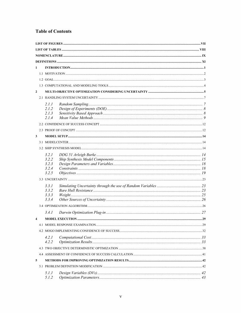
Table of Contents LIST OF FIGURES ................................................................................................................................................................................VII LIST OF TABLES ................................................................................................................................................................................ VIII NOMENCLATURE................................................................................................................................................................................. IX DEFINITIONS ......................................................................................................................................................................................... XI 1 INTRODUCTION...........................................................................................................................................................................1
1.1 MOTIVATION .................................................................................................................................................................................2
1.2 GOAL................................................................................................................................................................................................3
1.3 COMPUTATIONAL AND MODELING TOOLS..........................................................................................................................4
2 MULTI-OBJECTIVE OPTIMIZATION CONSIDERING UNCERTAINTY .......................................................................5 2.1 HANDLING SYSTEM UNCERTAINTY.......................................................................................................................................7
2.1.1 Random Sampling................................................................................................................... 7 2.1.2 Design of Experiments (DOE) ................................................................................................ 8 2.1.3 Sensitivity Based Approach .................................................................................................... 8 2.1.4 Mean Value Methods .............................................................................................................. 9
2.2 CONFIDENCE OF SUCCESS CONCEPT ...................................................................................................................................12
2.3 PROOF OF CONCEPT ..................................................................................................................................................................12
3 MODEL SETUP............................................................................................................................................................................14 3.1 MODELCENTER...........................................................................................................................................................................14
3.2 SHIP SYNTHESIS MODEL ..........................................................................................................................................................14
3.2.1 DDG 51 Arleigh Burke ......................................................................................................... 14 3.2.2 Ship Synthesis Model Components ....................................................................................... 15 3.2.3 Design Parameters and Variables........................................................................................ 18 3.2.4 Constraints ........................................................................................................................... 18 3.2.5 Objectives ............................................................................................................................. 19
3.3 UNCERTAINTY ............................................................................................................................................................................23
3.3.1 Simulating Uncertainty through the use of Random Variables ............................................ 23 3.3.2 Bare Hull Resistance ............................................................................................................ 23 3.3.3 Weight................................................................................................................................... 25 3.3.4 Other Sources of Uncertainty ............................................................................................... 26
3.4 OPTIMIZATION ALGORITHM...................................................................................................................................................26
3.4.1 Darwin Optimization Plug-in ............................................................................................... 27 4 MODEL EXECUTION ................................................................................................................................................................29
4.1 MODEL RESPONSE EXAMINATION........................................................................................................................................29
4.2 MOGO IMPLEMENTING CONFIDENCE OF SUCCESS..........................................................................................................32
4.2.1 Computational Cost .............................................................................................................. 33 4.2.2 Optimization Results............................................................................................................. 33
4.3 TWO OBJECTIVE DETERMINISTIC OPTIMIZATION ...........................................................................................................38
4.4 ASSESSMENT OF CONFIDENCE OF SUCCESS CALCULATION........................................................................................41
5 METHODS FOR IMPROVING OPTIMIZATION RESULTS..............................................................................................42 5.1 PROBLEM DEFINITION MODIFICATION ...............................................................................................................................42
5.1.1 Design Variables (DVs)........................................................................................................ 42 5.1.2 Optimization Parameters...................................................................................................... 43
vi
5.2 CONFIDENCE OF SUCCESS OBJECTIVE RESTRICTION.....................................................................................................47
5.3 SEGMENTED OPTIMIZATION RUNS.......................................................................................................................................50
5.4 PENALTY FUNCTIONS...............................................................................................................................................................53
5.5 RECOMMENDATIONS AND FINAL DPS FOR FURTHER EVALUATION .........................................................................57
5.5.1 Recommendations................................................................................................................. 57 5.5.2 Final DPs for Further Evaluation ........................................................................................ 58
6 HANDLING MULTIPLE SOURCES OF UNCERTAINTY ..................................................................................................61 6.1 CONFIDENCE OF SUCCESS CONCEPT EXTENDED TO MORE THAN TWO UNCERTAIN VARIABLES ...................61
6.2 MODEL EXECUTION WITH THREE UNCERTAIN RANDOM VARIABLES......................................................................63
6.2.1 CoS Calculation Validation.................................................................................................. 64 6.2.2 MOGO Implementing Confidence of Success....................................................................... 64
6.3 MODEL EXECUTION WITH FOUR UNCERTAIN RANDOM VARIABLES ........................................................................68
6.3.1 CoS Calculation Validation.................................................................................................. 68 6.3.2 MOGO Implementing Confidence of Success....................................................................... 68
6.4 MODEL EXECUTION WITH FOUR UNCERTAIN RANDOM VARIABLES REVISITED ..................................................72
6.4.1 Considering RT, Wls, KG, and KWmflm ............................................................................... 72 6.4.2 Considering RT, Wls, Atr, and E ........................................................................................... 73
6.5 OVERALL OBSERVATIONS ......................................................................................................................................................75
7 REFINING INDIVIDUAL DESIGNS ........................................................................................................................................76 7.1 DOT OPTIMIZATION TOOL.......................................................................................................................................................76
7.2 DOT OPTIMIZATION PROBLEM FORMULATION ................................................................................................................77
7.3 DOT RESULTS ..............................................................................................................................................................................78
8 NON-INTRUSIVE POLYNOMIAL CHAOS (NIPC) METHOD ..........................................................................................81 9 CONCLUSIONS ...........................................................................................................................................................................83 10 FUTURE WORK ..........................................................................................................................................................................85 REFERENCES..........................................................................................................................................................................................86 APPENDIX A: COS CALCULATION .................................................................................................................................................87 APPENDIX B: MODEL INPUT PARAMETERS, EXACT DDG 51 DP, AND DV BOUNDARIES............................................94 APPENDIX C: MOP WEIGHT VECTOR...........................................................................................................................................95 APPENDIX D: NUMERICAL DIFFERENTIATION CALCULATION CODED IN VISUAL BASIC SCRIPT ......................96 APPENDIX E: 2 VARIABLE COS CALCULATION CODED IN MATLAB ................................................................................98 APPENDIX F: 3 VARIABLE COS CALCULATION CODED IN MATLAB...............................................................................100 APPENDIX G: 4 VARIABLE COS CALCULATION CODED IN MATLAB..............................................................................102 APPENDIX H: PENALTY FUNCTION CODED IN MATLAB.....................................................................................................104 APPENDIX I: FINAL DPS FOR FURTHER EVALUATION ........................................................................................................106 APPENDIX J: SC DISCRETE DV DESIGN SPACE (STEPANCHICK AND BROWN, 2006) .................................................108 APPENDIX K: FINAL DPS FOR FURTHER EVALUATION AFTER DOT OPTIMIZATION ..............................................109
vii
List of Figures
Figure 1 - Naval Ship Design Process (Brown, 2006).................................................................................... 1 Figure 2 - Concept Exploration Process (Brown, 2006)................................................................................. 2 Figure 3 - Two Objective Attribute Space (Brown and Thomas, 1998)......................................................... 5 Figure 4 - Three Objective Attribute Space (Klasen, 2005) ........................................................................... 6 Figure 5 - JPDF in two variable standard normal space (Thacker et al., 2001)............................................ 10 Figure 6 - Objective Space scattered with Pareto Optimal DPs – from Klasen (2005) ................................ 13 Figure 7 - USS Arleigh Burke - DDG 51 (Doehring, 2006)......................................................................... 15 Figure 8 - Ship Synthesis Model in ModelCenter ........................................................................................ 15 Figure 9 - Naval Ship Acquisition Cost Components (Good and Brown, 2006).......................................... 20 Figure 10 - CoS GUI .................................................................................................................................... 22 Figure 11 - Bare Hull Resistance Comparison (Uncorrected) ...................................................................... 24 Figure 12 – DDG 51 PE Comparison (Uncorrected).................................................................................... 24 Figure 13 - Bare Hull Resistance Comparison (Corrected) .......................................................................... 25 Figure 14 - Multi-Objective Genetic Optimization (Stepanchick and Brown, 2006)................................... 27 Figure 15 - Darwin Optimization plug-in GUI............................................................................................. 28 Figure 16 - Criteria Responses in RV Space for DDG 51 DP – from Klasen (2005)................................... 30 Figure 17 - MCS and CoS LSFs of DDG 51 DP.......................................................................................... 32 Figure 18 - Three-Dimensional Scatter Plot of Pareto Optimal Design Solutions ....................................... 35 Figure 19 - Two-Dimensional Scatter Plot of Pareto Optimal Design Solutions ......................................... 36 Figure 20 - 2-D Scatter Plot of Pareto Front (Det. Infeasible and “Low” CoS DPs Removed) ................... 37 Figure 21 - Two Objective Deterministic Optimization Comparison........................................................... 38 Figure 22 – 3-D Scatter Plot of Pareto Optimal DPs using Updated Optimization Parameters ................... 45 Figure 23 – Original 3-D NDF (Reproduction of Figure 18) ....................................................................... 45 Figure 24 - 2-D Scatter Plot of Pareto Front using Updated Optimization Parameters ................................ 46 Figure 25 - 2-D Scatter Plot of Pareto Front using Updated Optimization Parameters (Det. Infeasible and
“Low” CoS DPs Removed)................................................................................................................. 47 Figure 26 - 3-D Scatter Plot of Pareto Optimal DPs with CoS Objective Constraint................................... 49 Figure 27 - 2-D Scatter Plot of Pareto Front with CoS Objective Constraint............................................... 50 Figure 28 - 3-D Scatter Plot of Piecewise Pareto Optimal DPs.................................................................... 52 Figure 29 - 2-D Scatter Plot of Piecewise Pareto Optimal DPs.................................................................... 53 Figure 30 - Penalty Function in MC Environment ....................................................................................... 55 Figure 31 - 3-D Scatter Plot of Pareto Optimal DPs using Penalty Function ............................................... 56 Figure 32 - 2-D Scatter Plot of Pareto Front using Penalty Function ........................................................... 57 Figure 33 - Logarithmically Divided Variable Space – from Klasen (2005) ............................................... 62 Figure 34 - CoS % Relative Error vs. # of Intervals in One Direction ......................................................... 63 Figure 35 - 3-D Scatter Plot of Pareto Optimal DPs considering 3 Uncertain RVs ..................................... 67 Figure 36 - 3-D Scatter Plot of Pareto Optimal DPs considering 4 Uncertain RVs ..................................... 71 Figure 37 - 3-D Scatter Plot of Pareto Optimal DPs considering 4 different RVs ....................................... 73 Figure 38 - 3-D Plot of Pareto Optimal DPs considering 4 different RVs Revisited ................................... 74 Figure 39 - DOT GUI................................................................................................................................... 76 Figure 40 - Plot of DOT Results for Final DPs ............................................................................................ 79
viii
List of Tables
Table 1 – Computational and Modeling Tools ............................................................................................... 4 Table 2 - CoS Calculation compared to MCS for DDG 51 DP – from Klasen (2005)................................. 13 Table 3 - Surface Combatant Design Variables............................................................................................ 18 Table 4 - Surface Combatant Design Constraints......................................................................................... 19 Table 5 - SWBS Weight Group RVs............................................................................................................ 26 Table 6 - Other Sources of Uncertainty........................................................................................................ 26 Table 7 - CoS Calculation compared to MCS for DDG 51 DP .................................................................... 31 Table 8 - Computational Cost of 2 Variable CoS Calculation...................................................................... 33 Table 9 - Possible Design Solutions ............................................................................................................. 35 Table 10 – Other Attractive Design Solutions.............................................................................................. 37 Table 11 - Two Objective Deterministic Optimization CoS Values ............................................................ 40 Table 12 - Probability Difference Between CoS and MCS for Pareto Optimal DPs.................................... 41 Table 13 - Design Variable Step Size Modification ..................................................................................... 43 Table 14 - Computational Cost using Updated Optimization Parameters .................................................... 44 Table 15 - Possible Design Solutions using Updated Optimization Parameters .......................................... 44 Table 16 - Other Attractive Design Solutions using Updated Optimization Parameters.............................. 46 Table 17 - Possible Design Solutions with CoS Objective Constraint ......................................................... 49 Table 18 - Other Attractive Design Solutions with CoS Objective Constraint............................................. 50 Table 19 - Computational Cost of Three Segmented Runs .......................................................................... 51 Table 20 - Possible Design Solutions using Piecewise Optimization........................................................... 52 Table 21 - Other Attractive Design Solutions using Piecewise Optimization .............................................. 53 Table 22 - Computational Cost using Penalty Function ............................................................................... 55 Table 23 - Possible Design Solutions using Penalty Function ..................................................................... 56 Table 24 – Other Attractive Design Solutions using Penalty Function ........................................................ 57 Table 25 - Universal Objective Extremes and DDG 51 DP ......................................................................... 59 Table 26 - Reproduction of "Best" DPs........................................................................................................ 59 Table 27 - Reproduction of "Knees" ............................................................................................................ 59 Table 28 - Final DPs Selected for Further Evaluation.................................................................................. 60 Table 29 - CoS Calculation compared to MCS for DDG 51 DP (3 Uncertain RVs).................................... 64 Table 30 - Uncertainties Analyzed in 3 Uncertain RVs Analysis................................................................. 65 Table 31 - Computational Cost using 3 Uncertain RVs ............................................................................... 66 Table 32 – Best Single Objective DPs considering 3 Uncertain RVs .......................................................... 67 Table 33 – Final DPs considering 3 Uncertain RVs..................................................................................... 67 Table 34 - CoS Calculation compared to MCS for DDG 51 DP (4 Uncertain RVs).................................... 68 Table 35 - Uncertainties Analyzed in 4 Uncertain RVs Analysis................................................................. 69 Table 36 - Computational Cost using 4 Uncertain RVs ............................................................................... 69 Table 37 - Computational Cost Data as a function of the number of RVs (* denotes projection) ............... 70 Table 38 – Best Single Objective DPs considering 4 Uncertain RVs .......................................................... 70 Table 39 – Final DPs considering 4 Uncertain RVs..................................................................................... 71 Table 40 - Uncertainties Analyzed in New 4 Uncertain RVs Analysis ........................................................ 72 Table 41 – Final DPs considering 4 Different Uncertain RVs ..................................................................... 73 Table 42 - Uncertainties Analyzed in New 4 Uncertain RVs Analysis ........................................................ 73 Table 43 – Final DPs considering 4 Different Uncertain RVs Revisited ..................................................... 74 Table 44 - Comparison of DDG 51 DPs....................................................................................................... 79 Table 45 - DOT Improvements for Final DPs .............................................................................................. 80 Table 46 - Potential Baseline Designs .......................................................................................................... 84
ix
Nomenclature
AAW Anti-Air Warfare AMV Advanced Mean Value Method AoA Analysis of Alternatives ASSET Advanced Surface Ship Evaluation Tool ASUW Anti-Surface Warfare ASW Anti-Submarine Warfare Atr Total Required Area B Beam at Waterline (m) BCC Basic Cost of Construction BHP Brake Horsepower CBR Chemical, Biological, and Radiological CDF Cumulative Distribution Function CFD Computational Fluid Dynamics CG Ticonderoga Class Cruiser CMan Manning Reduction Factor CoS Confidence of Success Cp Prismatic Coefficient CPS Collective Protection System Crd Raised Deck Coefficient CTOC Total Ownership Cost Cx Maximum Section Coefficient D10 Hull Depth at Station 10 (m) DDG Arleigh Burke Class Destroyer (Flights I/II/IIa) DDS Design Data Sheet DOE Design of Experiments DOT Design Optimization Tools DP Design Point DV Design Variable E Endurance Range FEM Finite Element Method FFG Oliver Hazard Perry Class Frigate GA Genetic Algorithm GUI Graphical User Interface IED Integrated Electric Drive JCDF Joint Cumulative Distribution Function JPDF Joint Probability Density Function KB Ship’s Overall Center of Buoyancy (m above keel) KG Ship’s Overall Center of Gravity (m above keel) KWmflm Maximum Functional Electrical Load with Margins LSF Limit State Function LWL Length at Waterline (m) MAV Multi-Attribute Value MC ModelCenter MCS Monte Carlo Simulation MDO Multi-Disciplinary Optimization
x
MOE Measure of Effectiveness MOFD Method of Feasible Directions MOGO Multi-Objective Genetic Optimization MOP Measure of Performance MPP Most Probable Point MPPL Most Probable Point Locus MV Mean Value Method NDF Non-Dominated Frontier NIPC Non-Intrusive Polynomial Chaos Method Ns Number of Ships to be Built NSWCCD Naval Surface Warfare Center – Carderock Division OMOE Overall Measure of Effectiveness ONR Office of Naval Research ORD Operational Requirements Document PC Polynomial Chaos PDF Probability Density Function PE Effective Power POE Projected Operational Environment ROCs Required Operational Capabilities RT Bare Hull Resistance RV Random Variable SC Surface Combatant SHP Shaft Horsepower SWBS Ship Work Breakdown Structure T Design Draft (m) USN United States Navy VCG Vertical Center of Gravity VD Deckhouse Volume (m3) VOP Value of Performance VT AOE Virginia Tech Dept. of Aerospace and Ocean Engineering Wls Lightship Weight WT Total Ship Weight Also note that SI units and abbreviations are used throughout this paper unless otherwise stated.
xi
Definitions
Attribute A quality or characteristic inherent to a particular design point; Attributes include design variables (i.e. beam), constraint performance values (i.e. sustained speed error value), and objectives (i.e. cost).
CDF Cumulative Distribution Function – the CDF of a
continuous random variable X with PDF f(x) is:
∫∞−
=≤=x
duufxXPxF )()()(
for -∞<x<∞ (Montgomery et al., 2004). Constraint An equality or inequality relation restricting the design
space; Constraints set minimum and/or maximum bounds on attributes.
Criterion An attribute used to make a decision in the design process,
such as a constraint performance value or objective. Design Point A vector of attributes that describes the characteristics of a
particular ship design. DPs may be dominated or non-dominated depending on their location relative to the Pareto front.
JPDF Joint Probability Density Function – the JPDF f(x,y) of two
continuous random variables X and Y is used to determine probabilities as follows:
∫ ∫=<<<<b
a
d
c
dydxyxfdYcbXaP ),(),(
for -∞<x<∞ and -∞<y<∞ (Montgomery et al., 2004). MDO Multi-Disciplinary Optimization – optimization that
integrates the multiple fields of ship design (i.e. hull geometry, resistance and propulsion, etc.).
MOGO Multi-Objective Genetic Optimization – evolutionary
optimization algorithm capable of handling nonlinear and multimodal optimization problems involving multiple objectives and constraints; based on Darwin’s principle of “survival of the fittest” (Benini, 2003).
xii
MOP Measure of Performance – specific ship or system performance metric independent of mission scenario or mission type, i.e. AAW, sustained speed, endurance range, etc. (Good and Brown, 2006).
NDF Non-Dominated Frontier – three-dimensional surface of
designs where each design represents the highest effectiveness for a given level of cost and CoS compared to other designs in the design space (Good and Brown, 2006).
Objective An attribute the designer wishes to optimize in the design
process, such as cost or effectiveness. OMOE Overall Measure of Effectiveness – quantitative measure of
a ship’s ability to perform over a range of mission types and mission scenarios. OMOE ranges from 0.0 to 1.0: an OMOE of 0.0 represents the least effective ship design possible in the given design space; an OMOE of 1.0 represents the most effective ship design possible in the given design space (Good and Brown, 2006).
Pareto Optimum A design solution on the non-dominated frontier (NDF). A
Pareto optimal design satisfies constraints such that no single objective can be improved without decreasing the performance of at least one other objective. A set of Pareto optimal design solutions is often referred to as a Pareto front or optimal set (Klasen, 2005).
PDF Probability Density Function – the PDF f(x) of a
continuous random variable X calculates probability according to the equation:
∫=<<b
a
dxxfbXaP )()(
for -∞<x<∞. A PDF must have the following properties:
f(x) ≥ 0 and ∫∞
∞−
= 1)(xf (Montgomery et al., 2004).
Ship Synthesis Model Set of interlinking multi-disciplinary modules used to
balance and assess the feasibility of each design selected during the optimization process. The ship synthesis model is composed of an input module, a nine module physics- based model, a constraint module, and three separate objective modules (Good et al., 2005).
xiii
VOP Value of Performance – quantitative measure of merit between 0.0 and 1.0 that specifies the value of a particular MOP to a specific mission area for a particular mission type (Good and Brown, 2006).
1
1 Introduction
The naval ship design approach has traditionally been an impromptu process, guided by experience, design lanes, rules of thumb, customer preference, and innovation. Using this approach, system objective attributes are rarely sufficiently quantified to make efficient and intelligent design decisions (Brown and Thomas, 1998). This thesis focuses on adding a third objective, uncertainty, to the effectiveness and cost objectives already present in a multi-disciplinary ship synthesis model. The aim is to use a total system approach for the naval ship design process by thoroughly searching the design space based on the multi-objective consideration of overall effectiveness and cost with an emphasis on the effects of uncertainty.
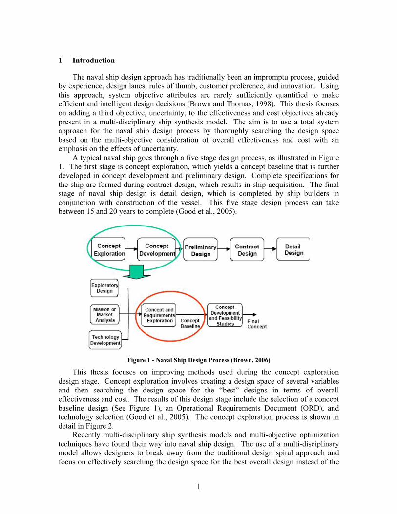
A typical naval ship goes through a five stage design process, as illustrated in Figure 1. The first stage is concept exploration, which yields a concept baseline that is further developed in concept development and preliminary design. Complete specifications for the ship are formed during contract design, which results in ship acquisition. The final stage of naval ship design is detail design, which is completed by ship builders in conjunction with construction of the vessel. This five stage design process can take between 15 and 20 years to complete (Good et al., 2005).
Figure 1 - Naval Ship Design Process (Brown, 2006)
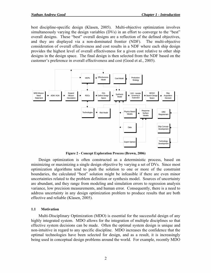
This thesis focuses on improving methods used during the concept exploration design stage. Concept exploration involves creating a design space of several variables and then searching the design space for the “best” designs in terms of overall effectiveness and cost. The results of this design stage include the selection of a concept baseline design (See Figure 1), an Operational Requirements Document (ORD), and technology selection (Good et al., 2005). The concept exploration process is shown in detail in Figure 2.
Recently multi-disciplinary ship synthesis models and multi-objective optimization techniques have found their way into naval ship design. The use of a multi-disciplinary model allows designers to break away from the traditional design spiral approach and focus on effectively searching the design space for the best overall design instead of the
Nathan Andrew Good Chapter 1 - Introduction
2
best discipline-specific design (Klasen, 2005). Multi-objective optimization involves simultaneously varying the design variables (DVs) in an effort to converge to the “best” overall designs. These “best” overall designs are a reflection of the defined objectives, and they are displayed via a non-dominated frontier (NDF). The multi-objective consideration of overall effectiveness and cost results in a NDF where each ship design provides the highest level of overall effectiveness for a given cost relative to other ship designs in the design space. The final design is then selected from the NDF based on the customer’s preference in overall effectiveness and cost (Good et al., 2005).
MNS Mission Need
StatementADM / AOA
Expand Mission
DescriptionROCs
DVsDefine Design
Space
Technologies
MOPs Effectiveness Model
Synthesis Model
Cost Model
Risk Model
Production Strategy
DOE - Variable Screening & Exploration
MOGOSearch Design
Space
Ship Acquisition Decision
ORDRequirement
Ship Concept Development
Technology Development
Physics Based Models
Data
Expert Opinion
Response Surface Models
Figure 2 - Concept Exploration Process (Brown, 2006)
Design optimization is often constructed as a deterministic process, based on minimizing or maximizing a single design objective by varying a set of DVs. Since most optimization algorithms tend to push the solution to one or more of the constraint boundaries, the calculated “best” solution might be infeasible if there are even minor uncertainties related to the problem definition or synthesis model. Sources of uncertainty are abundant, and they range from modeling and simulation errors to regression analysis variance, low precision measurements, and human error. Consequently, there is a need to address uncertainty in any design optimization problem to produce results that are both effective and reliable (Klasen, 2005). 1.1 Motivation
Multi-Disciplinary Optimization (MDO) is essential for the successful design of any highly integrated system. MDO allows for the integration of multiple disciplines so that effective system decisions can be made. Often the optimal system design is unique and non-intuitive in regard to any specific discipline. MDO increases the confidence that the optimal technologies have been selected for design, and as a result, it is increasingly being used in conceptual design problems around the world. For example, recently MDO
Nathan Andrew Good Chapter 1 - Introduction
3
has been used to reconfigure ship propulsion plants, to reduce the vehicle body weight of new cars, and to design hypersonic aircraft.
Complex integrated system design problems such as these often have high levels of uncertainty associated with their modeling and simulation, leading to the possibility that the selected design will not perform as well as expected. As a result, there is an increasing demand for a decision making tool that accounts for the effects of uncertainties in the design process. Uncertainty is typically handled using rough safety factors, but a probabilistic approach can produce results that are both more accurate and precise if the designer is willing to slightly increase analysis computational time (Klasen, 2005).
There are two main approaches for dealing with probabilistically formulated optimization problems: reliability based design and robust based design. Reliability based design is the more common of the two, and it focuses on satisfying the probabilistic constraints of the design problem (Klasen, 2005). In other words, reliability based design focuses on maximizing the probability that each design will be feasible and will not fail. Robust design focuses on designs that are less sensitive to the influence of uncontrollable factors; robust solutions optimize objectives while reducing variability (Mavris et al., 1998). However, even though robust design is considered very useful in making design decisions regarding complex engineering systems requiring MDO, its implementation is rare. One possible reason for this is the complexity and computational burden associated with evaluating objective variations due to uncertainties within the system (Du and Chen, 2002). 1.2 Goal
The goal of this work is to expand on the Confidence of Success (CoS) concept developed by Emanuel Klasen at Virginia Tech’s Department of Aerospace and Ocean Engineering (VT AOE). Klasen’s work explored the applicability and usability of the Mean Value method (MV) in analyzing system uncertainty in multi-objective optimization problems. Original implementation was performed on a simplified multi-disciplinary ship synthesis model developed at VT AOE. Klasen merged reliability based and robust based design approaches to quantify uncertainty using a calculation termed CoS. CoS is the probability that a specific ship design will satisfy all constraints and meet performance objectives (Klasen, 2005). For more information on Klasen’s original work, please see his report entitled “Confidence of Success in Multi-Criteria Optimization of Multi-Disciplinary Ship Design Models” (2005).
The original goal of the CoS concept was for it to be both fast and accurate enough to be applied to complex multi-disciplinary engineering systems with multiple objectives and heavy computational demands, yielding a CoS probability calculation for every feasible design point (DP). The probability calculation is performed utilizing the first steps of MV, using a basic Taylor series expansion to derive a Limit State Function (LSF) for each criterion response. Correlation between probabilistic criteria is handled through the simultaneous application of all LSFs to the Joint Probability Density Function (JPDF) of all uncertain variables (Klasen, 2005).
Klasen’s work proved that a concept such as CoS can be applied to a simple ship synthesis model to estimate system uncertainty early in the design process. However, a great deal of work remains to be done on this problem. This thesis aims to apply the CoS

Nathan Andrew Good Chapter 1 - Introduction
4
concept to a more detailed surface combatant synthesis model. In the original model, only two sources of uncertainty, resistance and weight, were considered. More sources of uncertainty need to be included, and all of these uncertainties need to be realistically quantified and represented in the model in order to investigate their relative importance to the overall design uncertainty or risk. Also, in the initial optimization effort, the DPs did not spread out well over the Pareto front. This work will attempt to penalize designs in the proximity of others to encourage a more uniform distribution of points across the front. Issues regarding optimizer performance with three objective functions in the presence of both discrete and continuous variables will also be examined. Once the Pareto front has been well defined, a particular design can be selected and refined using a gradient based optimization algorithm to minimize or maximize one of the objective functions while holding the others fixed. 1.3 Computational and Modeling Tools
Computational and modeling tools used in this project are listed in Table 1. ModelCenter version 6.1 and Analysis Server version 4.1 are modeling tools developed by Phoenix Integration. More information about these tools can be found at http://www.phoenix-int.com/.
Table 1 – Computational and Modeling Tools Application Software Package
Visual Design Environment ModelCenter 6.1 Module Wrapper Analysis Server 4.1 Primary Ship Synthesis Model Modules
Compaq Visual Fortran Standard Edition 6.1.0
Expansion Module Visual Basic MCS Script Visual Basic CoS Module Matlab 7.0.4 Surface Combatant Data ASSET
5
2 Multi-Objective Optimization Considering Uncertainty
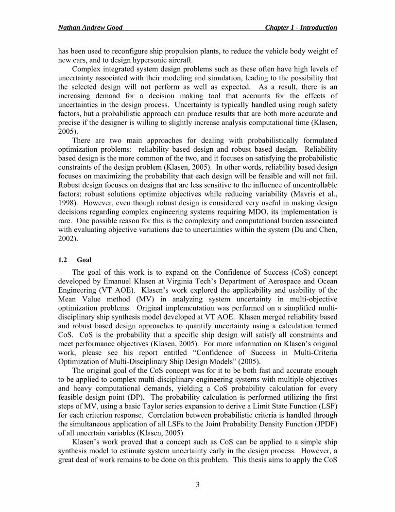
There is typically no single global optimum when performing multi-objective optimization because of tradeoffs between associated objectives. Conversely, multi-objective optimization results in a set of local Pareto optimums. A Pareto optimal design solution is a solution on the non-dominated frontier (NDF) that satisfies constraints such that no single objective can be improved without decreasing the performance of at least one other objective. A set of Pareto optimal design solutions is often referred to as a Pareto front or optimal set (Klasen, 2005). In this work, a NDF refers to a two-dimensional boundary or three-dimensional surface of designs where each design represents the highest effectiveness for a given level of cost and/or uncertainty compared to other designs in the design space (Good and Brown, 2006). Figure 3 displays a sample NDF in two objective attribute space. Here the objective is to minimize cost and maximize effectiveness in a deterministic multi-objective optimization process. The NDF is the boundary that separates the feasible and infeasible regions in the objective space. Every design solution in this objective space is represented by at least one design point (DP) in the design space, i.e. there is at least one design variable (DV) vector that results in the corresponding objectives (Klasen, 2005).
The decision of which design to use for the baseline design is ultimately left up to the customer, and it depends on their preference for particular objectives and the shape of the NDF itself. However, the customer should always choose a design that falls on the Pareto front. All other designs can be improved in at least one objective without being penalized in other objectives. Attractive design possibilities for the customer include designs at the extremes of the NDF and at “knees” in the curve or surface. Designs located at the “knees” of the NDF are of interest because of their sharp increase in, for example, effectiveness with a relatively small increase in cost and/or uncertainty (Good and Brown, 2006). The “knee” of the sample NDF is encircled in Figure 3.
Figure 3 - Two Objective Attribute Space (Brown and Thomas, 1998)
“Knee”
Nathan Andrew Good Chapter 2 – Multi-Objective Optimization Considering Uncertainty
6
Since most optimization algorithms tend to push the set of design solutions to one or more constraint boundaries, the baseline design selected from the NDF might be infeasible if there are even minor uncertainties associated with the problem definition or synthesis model. In a deterministic analysis, the probability that the baseline design will actually perform as predicted in terms of cost and effectiveness has not been considered. In reality, there is a great risk that the chosen design may under perform in terms of overall effectiveness, cost more than initially expected, or have a small chance of meeting constraint requirements. As a result, there is a need to address uncertainty in any design optimization problem to produce both effective and reliable results (Klasen, 2005).
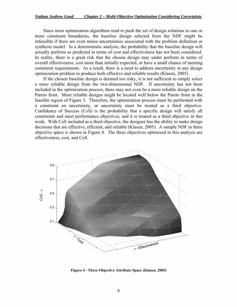
If the chosen baseline design is deemed too risky, it is not sufficient to simply select a more reliable design from the two-dimensional NDF. If uncertainty has not been included in the optimization process, there may not even be a more reliable design on the Pareto front. More reliable designs might be located well below the Pareto front in the feasible region of Figure 3. Therefore, the optimization process must be performed with a constraint on uncertainty, or uncertainty must be treated as a third objective. Confidence of Success (CoS) is the probability that a specific design will satisfy all constraints and meet performance objectives, and it is treated as a third objective in this work. With CoS included as a third objective, the designer has the ability to make design decisions that are effective, efficient, and reliable (Klasen, 2005). A sample NDF in three objective space is shown in Figure 4. The three objectives optimized in this analysis are effectiveness, cost, and CoS.
Figure 4 - Three Objective Attribute Space (Klasen, 2005)
Nathan Andrew Good Chapter 2 – Multi-Objective Optimization Considering Uncertainty
7
2.1 Handling System Uncertainty
Sources of system uncertainty are abundant, and they come from both qualitative and quantitative sources. Qualitative sources of uncertainty arise from categorical variables that cannot be measured on a well-defined numerical scale such as value, environmental impact, corrosion, skill, experience, and other human factors. In this work, the OMOE (Overall Measure of Effectiveness) function is based on a collection of categorical variables and is thus a source of qualitative uncertainty. Quantitative sources of uncertainty arise from modeling and simulation errors and statistical errors due to physical observation randomness. Physical observation randomness occurs when repeated measurements of the same physical parameter do not yield the same value due to instrument precision, environmental fluctuations, and human factors. When there is a large sample size, reliable information about the variability of the measured physical parameter can be obtained and statistical uncertainty is reduced. However, when the number of observations is limited, statistical uncertainty increases (Klasen, 2005).
This work focuses on analyzing the quantitative uncertainty associated with modeling and simulation errors. Modeling and simulation errors occur due to discrepancies between computational predictions and real world values. These errors are critical in the analysis of multi-disciplinary models such as a ship synthesis model due to interlinking modules. The computational output of one discipline is typically the input of another discipline, allowing a small initial uncertainty to grow as it progresses through the model. As a result, it is critical that system uncertainty is addressed in any optimization problem to ensure reliable results (Klasen, 2005).
There are a large number of different approaches devoted to handling system uncertainty. Most of these approaches can be classified into three categories: random sampling, design of experiments (DOE), and sensitivity based approaches. These three categories are briefly discussed in the following sections. The most efficient approach is strongly problem dependent, as there is typically a trade-off between accuracy and computational cost. For the multi-objective design optimization of a multi-disciplinary ship synthesis model, the system uncertainty approach of choice must have a low computational cost due the computational burden associated with a complex model and genetic optimization algorithm (GA). Therefore, the CoS calculation in this work is based only on the first steps of the Mean Value method (MV), i.e. a first order Taylor series expansion, classifying it as a sensitivity based approach. This method is discussed in greater detail in Section 2.1.4.3 (Klasen, 2005). 2.1.1 Random Sampling
The most famous and fundamental random sampling technique is Monte Carlo Simulation (MCS). MCS randomly generates values for uncertain variables over and over to simulate a model or process. MCS was named after Monte Carlo, Monaco, where the primary attraction is gambling in casinos via games of chance such as dice, roulette wheels, and slot machines. The random behavior of games such as these is very similar to how MCS selects random values for uncertain variables to simulate a model or process. Each variable has a known range of values and a probability distribution but an uncertain value at any moment in time (Decisioneering, 2005). MCS is considered to be
Nathan Andrew Good Chapter 2 – Multi-Objective Optimization Considering Uncertainty
8
the most accurate and precise method for calculating probability distributions of system responses with uncertainty. However, MCS typically calls for tens of thousands of system evaluations, leading to a computational cost too high for practical analysis of a multi-disciplinary ship synthesis model. For this reason, MCS is only used in this work as a means to compare CoS calculations and calculate CoS accuracy. MCS can be made more practical through the use of variance reduction techniques such as Descriptive Sampling and the Antithetic Variate technique (Klasen, 2005). 2.1.2 Design of Experiments (DOE)
A design of experiments (DOE) is an approach that establishes the relationship between parameters affecting a model or process and the output or response of that model or process. In DOE, a matrix is constructed in a structured and organized fashion that specifies the values for the uncertain variables for each sample DP. The possible values for the uncertain variables are defined by a range, a nominal baseline plus or minus a specified percent, or through specified discrete choices instead of using a probability distribution. Once the uncertain variable potential values have been defined, DOE evaluations can be performed. Each DOE evaluation is a combination of the defined potential values, resulting in a computational cost typically less than MCS. However, DOE approximations are typically less accurate than MCS approximations as well (Klasen, 2005). 2.1.3 Sensitivity Based Approach
A sensitivity analysis is a procedure used to determine the sensitivity of a system response to changes in system parameters, such as uncertain DVs. Sensitivity based approaches are typically based on first or second order Taylor series expansions. In sensitivity based approaches, response gradients are calculated at the mean values of the uncertain DVs instead of sampling across known probability distributions or ranges of uncertain DVs (Klasen, 2005).
Assuming that Z(X) is differentiable, the first-order Taylor series approximation for the performance response Z = Z(X) around the point μx is:
)()()(1
Xii
n
i i
XXZZZ μ
μ
−⋅⎟⎟⎠
⎞⎜⎜⎝
⎛∂∂
+≈ ∑=
xμX (1)
where μXi is the mean of uncertain variable i and n is the number of uncertain variables. When the uncertain variables, X, are set to their mean value μx, the expected value of Z can be calculated as: )()( xμZZE ≈ (2) The variance of Z is given by:
∑=
⋅⎟⎟⎠
⎞⎜⎜⎝
⎛∂∂
≈=n
iXi
iz X
ZZV1
22
2)( σσμ
(3)
where σXi is the standard deviation of uncertain variable i. A first order Taylor series expansion requires a minimum of (n+1) evaluations for
complete analysis. This approach is exceptionally accurate when performance responses are close to linear, and the computational cost is typically much lower than other methods
Nathan Andrew Good Chapter 2 – Multi-Objective Optimization Considering Uncertainty
9
such as MCS and DOE. For nonlinear response functions, a first order Taylor series expansion is generally not sufficiently accurate. When dealing with simple problems, higher-order Taylor series expansions can be used to improve the accuracy of the approximation. However, for problems involving a large number of uncertain variables, higher-order Taylor series expansions become difficult to obtain and inefficient as the computational cost increases significantly (Wu et al., 2002). For example, a second order Taylor series expansion requires (n+1)*(n+2)/2 evaluations for complete analysis (Klasen, 2005). 2.1.4 Mean Value Methods
Mean value methods utilize most probable point (MPP) analysis, and they are typically based on first order Taylor series expansions, classifying them as sensitivity based approaches. These methods are appropriate for “smooth” close to linear response functions that are computationally intensive (Thacker et al., 2001). As a result, mean value methods are used in the development of a CoS function used to analyze the uncertainty in a multi-disciplinary ship synthesis model.
Mean value methods approximate a cumulative distribution function (CDF) of the response function, which can be differentiated to obtain a probability density function (PDF). In the analysis, a response Z is defined as a function of the uncertain random variables X. Each point in the design space spanned by X has a specific probability density according to the joint probability density function (JPDF) of the uncertain random variables (RVs). Therefore every response value Z(X) has an associated probability density (Klasen, 2005).
These methods can also be used to perform parameter variation analysis, which is a useful tool to understand how the response functions vary with changes in the uncertain RVs. This has been implemented in the NESSUS probabilistic analysis software. More information about this software and mean value methods in general can be found in the NESSES Theoretical Manual (Southwest, 2001). 2.1.4.1 Limit State Function (LSF)
The limit state or failure surface that separates the design space into feasible and infeasible regions is g(X) = 0. For an arbitrary response function Z, g(X) is defined as:
0)()( =−= lsZZg XX (4) where the limit state value Zls is a specific value of the response function Z. Examples of an exact LSF and an approximate LSF can be seen in Figure 5. 2.1.4.2 Most Probable Point (MPP) Analysis
The most probable point (MPP) is defined as the point along the LSF where the uncertain variable combination yields the highest probability of occurrence. The first step in obtaining the MPP is approximating a LSF at the mean of the random uncertain variables. The original random uncertain variables must then be transformed into independent, normal RVs if they are not already. For a JPDF involving two standard normal and independent variables, the final step is to then calculate the minimum distance from the origin of the JPDF to the LSF. This point is identified as the MPP in standard normal space, and an example can be seen in Figure 5 (Thacker et al., 2001).
Nathan Andrew Good Chapter 2 – Multi-Objective Optimization Considering Uncertainty
10
For nonlinear limit states, identifying the MPP becomes an optimization problem in itself. Once the MPP has been identified, LSFs can be approximated at the MPP using polynomial functions (Klasen, 2005). 2.1.4.3 The Mean Value Method (MV)
As mentioned earlier, the Mean Value method (MV) is a sensitivity based approach based on a first order Taylor series expansion. Assuming the response function Z is “smooth” or can be “smoothed” and that a first order Taylor series expansion of Z exists at the mean μx of the uncertain variables X, the response function Z can be expressed as:
)()()()(1
XμX x HXXZZZ Xii
n
i i
+−⋅⎟⎟⎠
⎞⎜⎜⎝
⎛∂∂
+= ∑=
μμ
(5)
∑=
+−⋅+=n
iXiii HXaa
10 )()( Xμ (6)
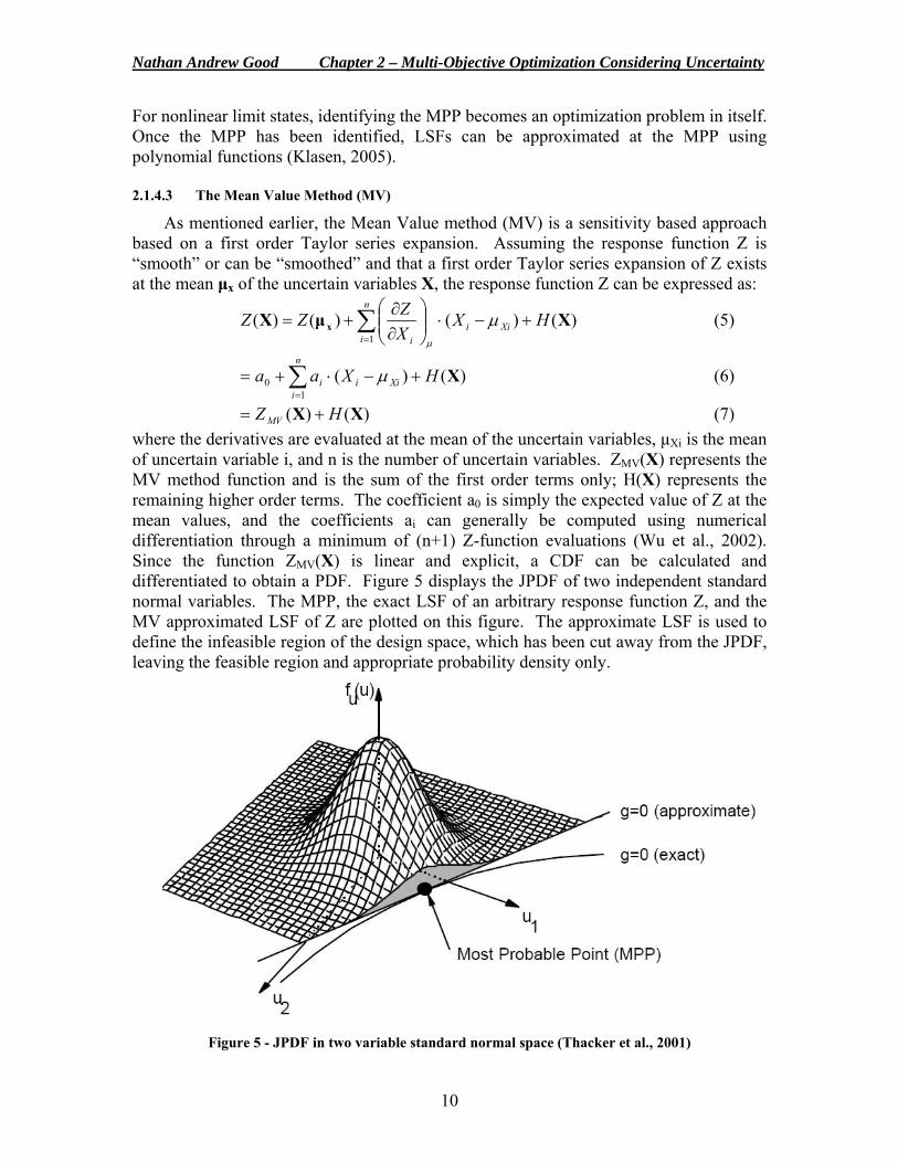
)()( XX HZ MV += (7) where the derivatives are evaluated at the mean of the uncertain variables, μXi is the mean of uncertain variable i, and n is the number of uncertain variables. ZMV(X) represents the MV method function and is the sum of the first order terms only; H(X) represents the remaining higher order terms. The coefficient a0 is simply the expected value of Z at the mean values, and the coefficients ai can generally be computed using numerical differentiation through a minimum of (n+1) Z-function evaluations (Wu et al., 2002). Since the function ZMV(X) is linear and explicit, a CDF can be calculated and differentiated to obtain a PDF. Figure 5 displays the JPDF of two independent standard normal variables. The MPP, the exact LSF of an arbitrary response function Z, and the MV approximated LSF of Z are plotted on this figure. The approximate LSF is used to define the infeasible region of the design space, which has been cut away from the JPDF, leaving the feasible region and appropriate probability density only.
Figure 5 - JPDF in two variable standard normal space (Thacker et al., 2001)
Nathan Andrew Good Chapter 2 – Multi-Objective Optimization Considering Uncertainty
11
For nonlinear response functions, the first order Taylor series expansion approximation of MV is generally not sufficiently accurate. When dealing with simple problems, increasing the order of the Taylor series expansion can improve the accuracy of the approximation. However, for problems involving a large number of uncertain variables, higher-order Taylor series expansions become unattractive since they are difficult to obtain and inefficient as the computational cost increases significantly. The Advanced Mean Value method (AMV) described in the following section provides an alternative that improves upon the MV solution with a minimum number of additional Z-function evaluations (Wu et al., 2002). 2.1.4.4 The Advanced Mean Value Method (AMV)
The Advanced Mean Value method (AMV) improves upon the MV solution by introducing a simple correction procedure used to compensate for the errors associated with the truncation of the Taylor series expansion. The AMV model is defined as: )( MVMVAMV ZHZZ += (8) where H(ZMV) is defined as the difference between the calculated values of Z and ZMV at the Most Probable Point Locus (MPPL) of ZMV. The MPPL is defined by connecting the MPPs for different values of Zls. AMV reduces the truncation error by replacing the higher-order terms of the Taylor series expansion with a simplified function H(ZMV). The truncation error is still not optimum due to this approximation, but the MV generated MPPs are typically close to the exact MPPs, making AMV a reasonably good solution.
AMV can also provide information about the non-linear properties of the LSF to identify potential problems. However, assuming that a numerical differentiation scheme is used to define ZMV, the required number of Z-function evaluations increases from (n+1) to (n+1+m), where n is the number of random uncertain variables and m is the number of CDF levels used for the correction of the MV generated CDF (Wu et al., 2002). Due to the extra evaluations associated with AMV, a CoS calculation based only on MV is used in this work when linear approximations are applicable. 2.1.4.5 Linear Dependence
It has been suggested that a probabilistic approach to handling uncertainties could lead to very accurate multi-objective design optimization. However, the handling of uncertainties in such a complicated optimization process can become very complex. It is inadequate to simply look at each criterion and its associated distribution independently due to the fact that all design attributes are interdependent. Therefore, one cannot assume that criteria are independent of each other, and a method of measuring correlation is needed (Klasen, 2005).
One linear relationship between multiple RVs is called covariance, and it is defined as: )()()(),( YEXEXYEYXCov −= (9) where X and Y are RVs. When X and Y are independent of each other, the covariance is equal to zero. When the covariance is not equal to zero, there is a relationship between X and Y. The covariance is closely related to the correlation between the random variables X and Y. Correlation is defined as:
Nathan Andrew Good Chapter 2 – Multi-Objective Optimization Considering Uncertainty
12
22
),(
YX
XYYXCov
σσρ = (10)
where ρXY is termed the correlation coefficient and ranges from -1 to +1. A correlation coefficient of exactly 1 indicates perfect positive linear dependence. This means that as Y increases, X also increases. A correlation coefficient of exactly -1 indicates perfect negative linear dependence. This means that as Y increases, X decreases. The correlation coefficient is expected to be close to zero if the RVs are independent of each other. In general, perfect positive/negative linear dependence or perfect linear independence is rare. Therefore, the correlation between two variables is considered strong when the correlation coefficient is between 0.8 and 1, weak when the correlation coefficient is between 0 and 0.5, and moderate otherwise.
2.2 Confidence of Success Concept
The initial Confidence of Success (CoS) concept, and its calculation for two uncertain variables, was developed by Emanuel Klasen (2005) at VT AOE. The concept is described in detail in Appendix A, and the two variable Matlab code is presented with comments in Appendix E. 2.3 Proof of Concept
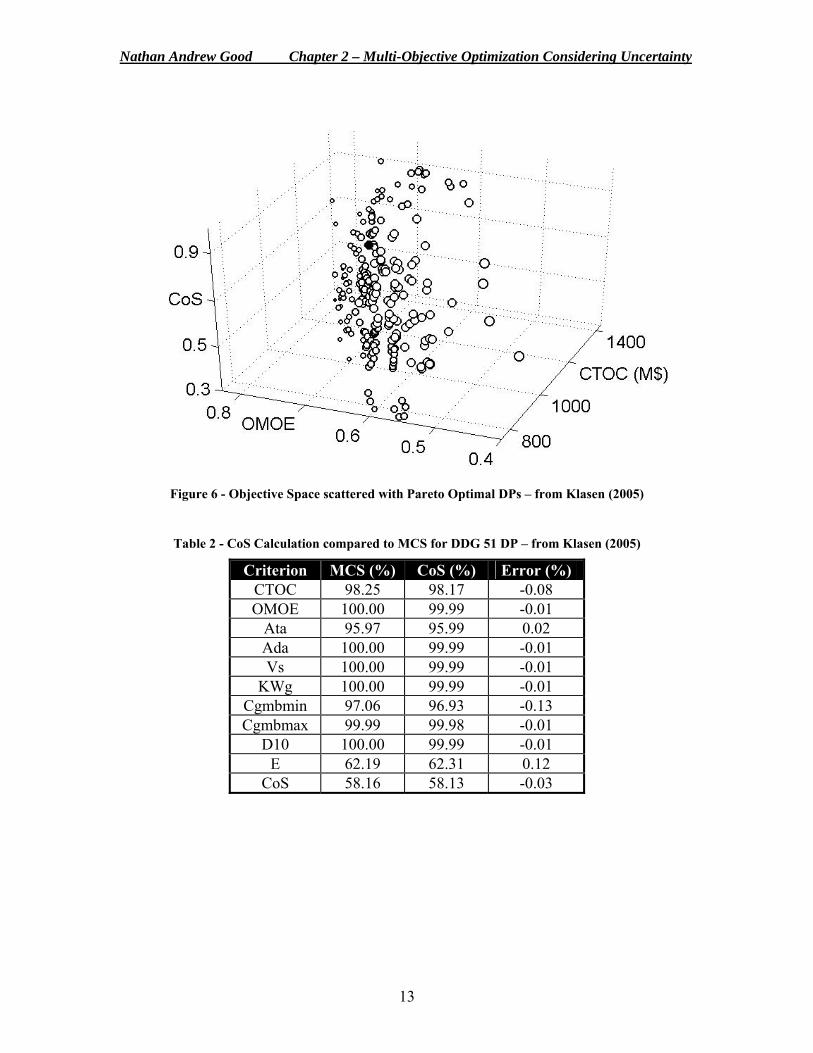
The applicability and usability of Klasen’s CoS calculation was investigated through its implementation in the optimization of a simplified multi-disciplinary ship synthesis model. The optimization process concluded after 70 hours of searching the objective space for non-dominated designs due to lack of improvement. The optimization process examined 215 generations, each with a population of 300 individual designs. There were a total of 46,079 deterministic infeasible and 18,422 deterministic feasible designs evaluated in the optimization process. Of these thousands of designs, 260 design solutions were preserved for the construction of the Pareto front, which is presented in Figure 6 as a three-dimensional scatter plot. Validation of the CoS calculation was performed by comparing a CoS and MCS calculation (100,000 system evaluations) for the DDG 51 DP and other random DPs (Klasen, 2005). The DDG 51 DP is described in detail in Section 3.2.1 and Appendix B. The results for the DDG 51 DP are shown in Table 2. The criteria listed in Table 2 include the three objectives (CTOC, OMOE, and CoS) as well as the eight constraints used by Klasen, which are described in greater detail in Section 3.2.4. Percentages represent the probability of feasibility for each specific criterion. For more details about Klasen’s results, please see Chapter 5 of his paper “Confidence of Success in Multi-Criteria Optimization of Multi-Disciplinary Ship Design Models” (2005).
Nathan Andrew Good Chapter 2 – Multi-Objective Optimization Considering Uncertainty
13
Figure 6 - Objective Space scattered with Pareto Optimal DPs – from Klasen (2005)
Table 2 - CoS Calculation compared to MCS for DDG 51 DP – from Klasen (2005)
Criterion MCS (%) CoS (%) Error (%) CTOC 98.25 98.17 -0.08 OMOE 100.00 99.99 -0.01
Ata 95.97 95.99 0.02 Ada 100.00 99.99 -0.01 Vs 100.00 99.99 -0.01
KWg 100.00 99.99 -0.01 Cgmbmin 97.06 96.93 -0.13 Cgmbmax 99.99 99.98 -0.01
D10 100.00 99.99 -0.01 E 62.19 62.31 0.12
CoS 58.16 58.13 -0.03
14
3 Model Setup
Multi-objective design optimization considering uncertainty via a CoS calculation was performed using a multi-disciplinary ship synthesis model. Hardware used for this computation intensive task was a twin-processor Dell PSW650: Xeon 2x2.66 GHz CPU, 1.0 GB RAM. The ship synthesis model is described in greater detail later in this Chapter.
3.1 ModelCenter
ModelCenter version 6.1 is a commercial process integration and design optimization software package developed by Phoenix Integration, Inc. used to build and execute complex engineering models. ModelCenter (MC) provides a visual environment in which design processes can be assembled as a series of linked applications with a single interface in order to easily perform multi-disciplinary analysis. MC automatically connects design data from one application to the next, producing an automated multi-disciplinary design environment. More information about MC can be found at http://www.phoenix-int.com/. 3.2 Ship Synthesis Model
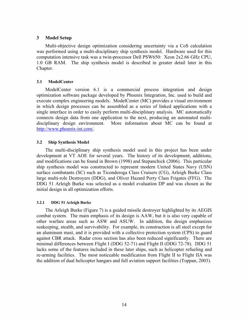
The multi-disciplinary ship synthesis model used in this project has been under development at VT AOE for several years. The history of its development, additions, and modifications can be found in Brown (1998) and Stepanchick (2006). This particular ship synthesis model was constructed to represent modern United States Navy (USN) surface combatants (SC) such as Ticonderoga Class Cruisers (CG), Arleigh Burke Class large multi-role Destroyers (DDG), and Oliver Hazard Perry Class Frigates (FFG). The DDG 51 Arleigh Burke was selected as a model evaluation DP and was chosen as the initial design in all optimization efforts. 3.2.1 DDG 51 Arleigh Burke
The Arleigh Burke (Figure 7) is a guided missile destroyer highlighted by its AEGIS combat system. The main emphasis of its design is AAW, but it is also very capable of other warfare areas such as ASW and ASUW. In addition, the design emphasizes seakeeping, stealth, and survivability. For example, its construction is all steel except for an aluminum mast, and it is provided with a collective protection system (CPS) to guard against CBR attack. Radar cross section has also been reduced significantly. There are minimal differences between Flight I (DDG 52-71) and Flight II (DDG 72-78). DDG 51 lacks some of the features included in these later ships, such as helicopter refueling and re-arming facilities. The most noticeable modification from Flight II to Flight IIA was the addition of dual helicopter hangars and full aviation support facilities (Toppan, 2003).
Nathan Andrew Good Chapter 3 – Model Setup
15
Figure 7 - USS Arleigh Burke - DDG 51 (Doehring, 2006)
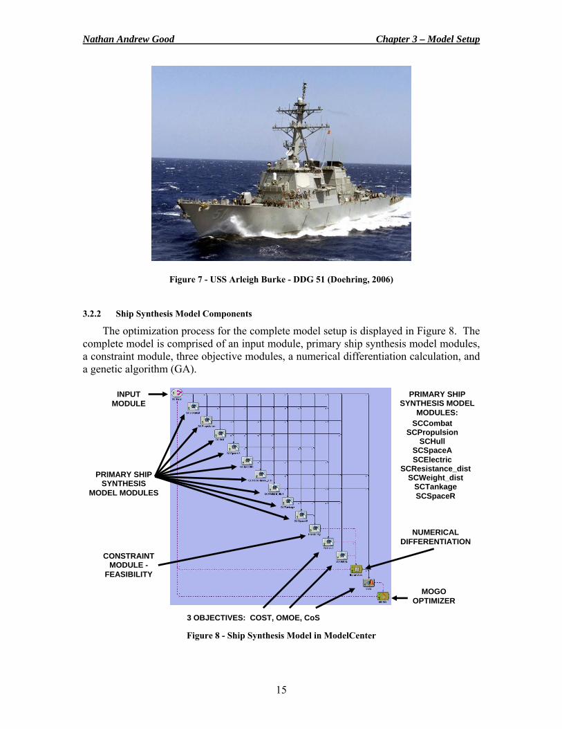
3.2.2 Ship Synthesis Model Components
The optimization process for the complete model setup is displayed in Figure 8. The complete model is comprised of an input module, primary ship synthesis model modules, a constraint module, three objective modules, a numerical differentiation calculation, and a genetic algorithm (GA).
Figure 8 - Ship Synthesis Model in ModelCenter
INPUT MODULE
PRIMARY SHIP SYNTHESIS
MODEL MODULES
CONSTRAINT MODULE -
FEASIBILITY
3 OBJECTIVES: COST, OMOE, CoS
MOGO OPTIMIZER
PRIMARY SHIP SYNTHESIS MODEL
MODULES: SCCombat
SCPropulsion SCHull
SCSpaceA SCElectric
SCResistance_dist SCWeight_dist
SCTankage SCSpaceR
NUMERICAL DIFFERENTIATION
Nathan Andrew Good Chapter 3 – Model Setup
16
The primary ship synthesis model is comprised of several interlinked modules, each focusing on one specific discipline, such as propulsion, hullform, or resistance. Modules can easily be added or removed in the MC environment, allowing the model to more accurately represent the mission definition. All modules in this model are coded in Fortran, but MC also has Excel, Mathcad, and Matlab plug-ins. In addition, integration software allows calculations from other applications, such as CFD or FEM, to be included (Klasen, 2005). ASSET can also be integrated into the MC environment.
Each individual design is balanced in the Weight and Stability Module using the fuel weight parameter. All weights considered in the model are summed to determine the ship’s overall weight without fuel. Fuel weight is then calculated as the difference between the calculated weights without fuel and the ship’s displacement. Each balanced design’s attributes are then compared to the functional requirements of the design. These requirements arise due to constraints, such as sustained speed and endurance range, placed on each design. There is no iterative design balancing; each individual design either fulfills requirements or does not and is deemed either feasible or infeasible. All infeasible designs are penalized by the optimizer, causing a thorough search of the entire design space for feasible solutions. In addition, CoS is automatically set to zero for infeasible DPs, eliminating unnecessary iterations and computational work required for probability calculations (Klasen, 2005).
All model components except for the numerical differentiation calculation, probability calculation, and GA are described below. These other components are described in greater detail later this Chapter. It should also be noted that each module is much more detailed than presented in this work. This report simply gives a brief overview of the model so that the results can be better understood. More information about the model itself can be obtained from Dr. Alan Brown at VT AOE.
• Input Module – Compiles, interprets, and processes the input DVs and other
design parameters. The Input Module is linked to all of the other modules. • Combat Systems Module – Calculates payload characteristics such as SWBS
weight, vertical center of gravity, area, and power for each combat system combination based on the selected DVs from the Input Module and data from the Combat Systems Database. Combat Systems DVs include AAW, ASUW, ASW, CCC, NSFS, SEW, GMLS, SDS, and LAMPS.
• Propulsion Module – Retrieves propulsion characteristics for a specific system from the Propulsion System Database and calculates propulsive efficiency based on the propulsion system DV. Information in the Propulsion System Database is based on manufacturer data and ASSET calculations.
• Hullform Module – Uses inputs to calculate total hull surface area, full load displaced volume, sonar dome information, and other basic hullform coefficients.
• Space Available Module – Uses naval architecture analyses to calculate available space dimensions. Inputs include basic hullform characteristics, deck house volume, full load displacement volume, machinery box characteristics, number of propulsors, and hull flare angle. Outputs include total hull volume, hull cubic number, total ship volume, and actual machinery box dimensions.
• Electric Power Module – Uses data from the other modules and parametric equations with margins to estimate the ship power requirements with margins.
Nathan Andrew Good Chapter 3 – Model Setup
17
This module assumes one ship service generator is unavailable, uses a power factor of 0.9, and uses the electric load analysis method from DDS 310-1. Ship manpower requirements are also calculated in this module using regression-based equations (Stepanchick and Brown, 2006).
• Resistance Module – Utilizes the Holtrop-Mennen method (Holtrop, 1984) to calculate the bare hull resistance of each ship design. Wind resistance and appendage resistance are also calculated and added to the bare hull resistance to calculate total resistance and effective power. The propulsive coefficient used in this module is approximated, and sustained speed is calculated based on total BHP available with a 25% margin. Outputs of this module include SHP required, sustained speed, and propeller diameter (Stepanchick and Brown, 2006).
• Weight and Stability Module – Uses inputs and parametric equations to evaluate SWBS weights and calculate the overall ship weight without fuel. Available fuel weight is then the difference between the calculated overall ship weight without fuel and the full load displacement. Individual weights and their respective vertical centers of gravity (VCGs) are used to determine the overall ship center of gravity (KG). Other outputs include full load displacement, lightship weight (Wls), SWBS weights, load characteristics, center of buoyancy (KB), and the GM/B ratio.
• Tankage Module – Calculates total tank volume, propulsion fuel tank volume, endurance range, and gallons of fuel used per year. The propulsion fuel tank volume is calculated using the calculated fuel weight from the Weight and Stability Module, and other tankage such as ballast, water, sewage, and waste tanks are calculated using parametric equations. The fuel tankage calculation is based on DDS-200-1.
• Space Required Module – Calculates the total space required using parametric equations. Inputs include hullform characteristics, total tankage volume, machinery volume, total hull volume, payload area, inlet and exhaust area, endurance days, hull cubic number, and manning requirements. Outputs include both required and available hull and deck house areas.
• Feasibility Module – Determines the overall feasibility of each SC design by comparing available design parameters to required design parameters. This constraint module is described in more detail in Section 3.2.4.
• Cost Module – Calculates lead ship acquisition cost, average follow ship acquisition cost, and follow ship total ownership cost (CTOC) using a weight-based cost model. This objective module is described in more detail in Section 3.2.5.1.
• Effectiveness Module – Calculates the Value of Performance (VOP) for each Measure of Performance (MOP) such as Anti-Air Warfare (AAW), Intelligence, and Sustained Speed. The dot product of this specific VOP vector and the MOP weight vector generates an OMOE value between 0 and 1 for a particular ship design. This objective module is described in more detail in Section 3.2.5.2.
Nathan Andrew Good Chapter 3 – Model Setup
18
3.2.3 Design Parameters and Variables
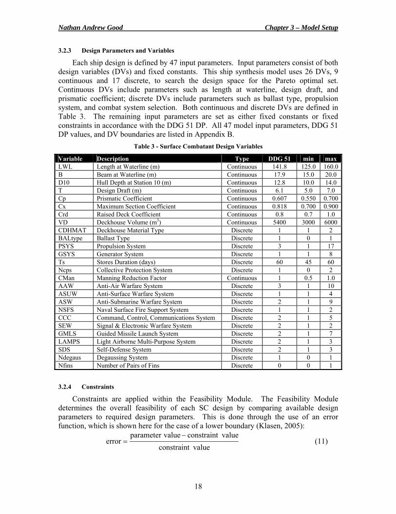
Each ship design is defined by 47 input parameters. Input parameters consist of both design variables (DVs) and fixed constants. This ship synthesis model uses 26 DVs, 9 continuous and 17 discrete, to search the design space for the Pareto optimal set. Continuous DVs include parameters such as length at waterline, design draft, and prismatic coefficient; discrete DVs include parameters such as ballast type, propulsion system, and combat system selection. Both continuous and discrete DVs are defined in Table 3. The remaining input parameters are set as either fixed constants or fixed constraints in accordance with the DDG 51 DP. All 47 model input parameters, DDG 51 DP values, and DV boundaries are listed in Appendix B.
Table 3 - Surface Combatant Design Variables
Variable Description Type DDG 51 min max LWL Length at Waterline (m) Continuous 141.8 125.0 160.0B Beam at Waterline (m) Continuous 17.9 15.0 20.0 D10 Hull Depth at Station 10 (m) Continuous 12.8 10.0 14.0 T Design Draft (m) Continuous 6.1 5.0 7.0 Cp Prismatic Coefficient Continuous 0.607 0.550 0.700Cx Maximum Section Coefficient Continuous 0.818 0.700 0.900Crd Raised Deck Coefficient Continuous 0.8 0.7 1.0 VD Deckhouse Volume (m3) Continuous 5400 3000 6000 CDHMAT Deckhouse Material Type Discrete 1 1 2 BALtype Ballast Type Discrete 1 0 1 PSYS Propulsion System Discrete 3 1 17 GSYS Generator System Discrete 1 1 8 Ts Stores Duration (days) Discrete 60 45 60 Ncps Collective Protection System Discrete 1 0 2 CMan Manning Reduction Factor Continuous 1 0.5 1.0 AAW Anti-Air Warfare System Discrete 3 1 10 ASUW Anti-Surface Warfare System Discrete 1 1 4 ASW Anti-Submarine Warfare System Discrete 2 1 9 NSFS Naval Surface Fire Support System Discrete 1 1 2 CCC Command, Control, Communications System Discrete 2 1 5 SEW Signal & Electronic Warfare System Discrete 2 1 2 GMLS Guided Missile Launch System Discrete 2 1 7 LAMPS Light Airborne Multi-Purpose System Discrete 2 1 3 SDS Self-Defense System Discrete 2 1 3 Ndegaus Degaussing System Discrete 1 0 1 Nfins Number of Pairs of Fins Discrete 0 0 1 3.2.4 Constraints
Constraints are applied within the Feasibility Module. The Feasibility Module determines the overall feasibility of each SC design by comparing available design parameters to required design parameters. This is done through the use of an error function, which is shown here for the case of a lower boundary (Klasen, 2005):
valueconstraintvalueconstraintvalueparameter
error−
= (11)
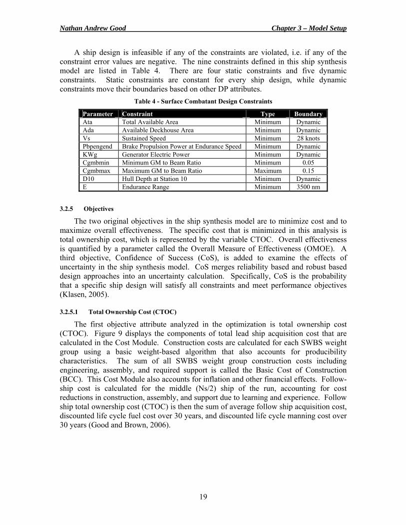
Nathan Andrew Good Chapter 3 – Model Setup
19
A ship design is infeasible if any of the constraints are violated, i.e. if any of the constraint error values are negative. The nine constraints defined in this ship synthesis model are listed in Table 4. There are four static constraints and five dynamic constraints. Static constraints are constant for every ship design, while dynamic constraints move their boundaries based on other DP attributes.
Table 4 - Surface Combatant Design Constraints
Parameter Constraint Type Boundary Ata Total Available Area Minimum Dynamic Ada Available Deckhouse Area Minimum Dynamic Vs Sustained Speed Minimum 28 knots Pbpengend Brake Propulsion Power at Endurance Speed Minimum Dynamic KWg Generator Electric Power Minimum Dynamic Cgmbmin Minimum GM to Beam Ratio Minimum 0.05 Cgmbmax Maximum GM to Beam Ratio Maximum 0.15 D10 Hull Depth at Station 10 Minimum Dynamic E Endurance Range Minimum 3500 nm
3.2.5 Objectives
The two original objectives in the ship synthesis model are to minimize cost and to maximize overall effectiveness. The specific cost that is minimized in this analysis is total ownership cost, which is represented by the variable CTOC. Overall effectiveness is quantified by a parameter called the Overall Measure of Effectiveness (OMOE). A third objective, Confidence of Success (CoS), is added to examine the effects of uncertainty in the ship synthesis model. CoS merges reliability based and robust based design approaches into an uncertainty calculation. Specifically, CoS is the probability that a specific ship design will satisfy all constraints and meet performance objectives (Klasen, 2005). 3.2.5.1 Total Ownership Cost (CTOC)
The first objective attribute analyzed in the optimization is total ownership cost (CTOC). Figure 9 displays the components of total lead ship acquisition cost that are calculated in the Cost Module. Construction costs are calculated for each SWBS weight group using a basic weight-based algorithm that also accounts for producibility characteristics. The sum of all SWBS weight group construction costs including engineering, assembly, and required support is called the Basic Cost of Construction (BCC). This Cost Module also accounts for inflation and other financial effects. Follow-ship cost is calculated for the middle (Ns/2) ship of the run, accounting for cost reductions in construction, assembly, and support due to learning and experience. Follow ship total ownership cost (CTOC) is then the sum of average follow ship acquisition cost, discounted life cycle fuel cost over 30 years, and discounted life cycle manning cost over 30 years (Good and Brown, 2006).
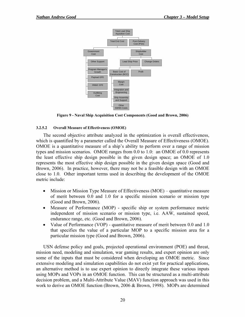
Nathan Andrew Good Chapter 3 – Model Setup
20
Other Support
Program Manager'sGrowth
Payload GFE
HM&E GFE
OutfittingCost
GovernmentCost
MarginCost
Integration andEngineering
Ship Assemblyand Support
OtherSWBS Costs
Basic Cost ofConstruction (BCC)
Profit
Lead Ship Price Change Orders
ShipbuilderCost
Total End Cost Post-DeliveryCost (PSA)
Total Lead ShipAquisition Cost
Figure 9 - Naval Ship Acquisition Cost Components (Good and Brown, 2006)
3.2.5.2 Overall Measure of Effectiveness (OMOE)
The second objective attribute analyzed in the optimization is overall effectiveness, which is quantified by a parameter called the Overall Measure of Effectiveness (OMOE). OMOE is a quantitative measure of a ship’s ability to perform over a range of mission types and mission scenarios. OMOE ranges from 0.0 to 1.0: an OMOE of 0.0 represents the least effective ship design possible in the given design space; an OMOE of 1.0 represents the most effective ship design possible in the given design space (Good and Brown, 2006). In practice, however, there may not be a feasible design with an OMOE close to 1.0. Other important terms used in describing the development of the OMOE metric include:
• Mission or Mission Type Measure of Effectiveness (MOE) – quantitative measure
of merit between 0.0 and 1.0 for a specific mission scenario or mission type (Good and Brown, 2006).
• Measure of Performance (MOP) - specific ship or system performance metric independent of mission scenario or mission type, i.e. AAW, sustained speed, endurance range, etc. (Good and Brown, 2006).
• Value of Performance (VOP) - quantitative measure of merit between 0.0 and 1.0 that specifies the value of a particular MOP to a specific mission area for a particular mission type (Good and Brown, 2006).
USN defense policy and goals, projected operational environment (POE) and threat,
mission need, modeling and simulation, war gaming results, and expert opinion are only some of the inputs that must be considered when developing an OMOE metric. Since extensive modeling and simulation capabilities do not exist yet for practical applications, an alternative method is to use expert opinion to directly integrate these various inputs using MOPs and VOPs in an OMOE function. This can be structured as a multi-attribute decision problem, and a Multi-Attribute Value (MAV) function approach was used in this work to derive an OMOE function (Brown, 2006 & Brown, 1998). MOPs are determined
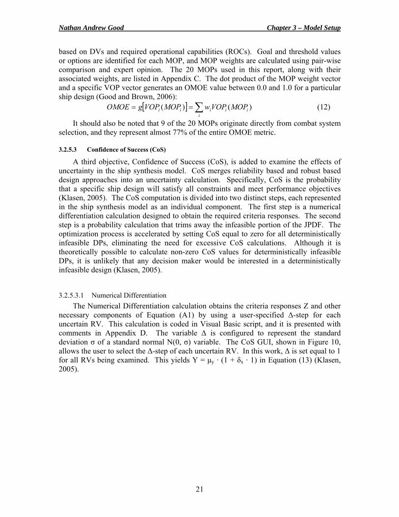
Nathan Andrew Good Chapter 3 – Model Setup
21
based on DVs and required operational capabilities (ROCs). Goal and threshold values or options are identified for each MOP, and MOP weights are calculated using pair-wise comparison and expert opinion. The 20 MOPs used in this report, along with their associated weights, are listed in Appendix C. The dot product of the MOP weight vector and a specific VOP vector generates an OMOE value between 0.0 and 1.0 for a particular ship design (Good and Brown, 2006):
[ ] ∑==i
iiiii MOPVOPwMOPVOPgOMOE )()( (12)
It should also be noted that 9 of the 20 MOPs originate directly from combat system selection, and they represent almost 77% of the entire OMOE metric. 3.2.5.3 Confidence of Success (CoS)
A third objective, Confidence of Success (CoS), is added to examine the effects of uncertainty in the ship synthesis model. CoS merges reliability based and robust based design approaches into an uncertainty calculation. Specifically, CoS is the probability that a specific ship design will satisfy all constraints and meet performance objectives (Klasen, 2005). The CoS computation is divided into two distinct steps, each represented in the ship synthesis model as an individual component. The first step is a numerical differentiation calculation designed to obtain the required criteria responses. The second step is a probability calculation that trims away the infeasible portion of the JPDF. The optimization process is accelerated by setting CoS equal to zero for all deterministically infeasible DPs, eliminating the need for excessive CoS calculations. Although it is theoretically possible to calculate non-zero CoS values for deterministically infeasible DPs, it is unlikely that any decision maker would be interested in a deterministically infeasible design (Klasen, 2005).
3.2.5.3.1 Numerical Differentiation The Numerical Differentiation calculation obtains the criteria responses Z and other
necessary components of Equation (A1) by using a user-specified Δ-step for each uncertain RV. This calculation is coded in Visual Basic script, and it is presented with comments in Appendix D. The variable Δ is configured to represent the standard deviation σ of a standard normal N(0, σ) variable. The CoS GUI, shown in Figure 10, allows the user to select the Δ-step of each uncertain RV. In this work, Δ is set equal to 1 for all RVs being examined. This yields Y = μy · (1 + δx · 1) in Equation (13) (Klasen, 2005).
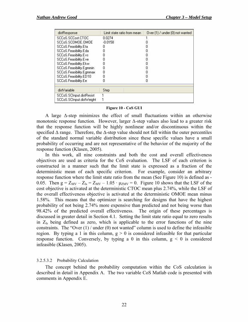
Nathan Andrew Good Chapter 3 – Model Setup
22
Figure 10 - CoS GUI
A large Δ-step minimizes the effect of small fluctuations within an otherwise monotonic response function. However, larger Δ-step values also lead to a greater risk that the response function will be highly nonlinear and/or discontinuous within the specified Δ range. Therefore, the Δ-step value should not fall within the outer percentiles of the standard normal variable distribution since these specific values have a small probability of occurring and are not representative of the behavior of the majority of the response function (Klasen, 2005).
In this work, all nine constraints and both the cost and overall effectiveness objectives are used as criteria for the CoS evaluation. The LSF of each criterion is constructed in a manner such that the limit state is expressed as a fraction of the deterministic mean of each specific criterion. For example, consider an arbitrary response function where the limit state ratio from the mean (See Figure 10) is defined as -0.05. Then g = ZMV – Zls = ZMV – 1.05 · μZMV = 0. Figure 10 shows that the LSF of the cost objective is activated at the deterministic CTOC mean plus 2.74%, while the LSF of the overall effectiveness objective is activated at the deterministic OMOE mean minus 1.58%. This means that the optimizer is searching for designs that have the highest probability of not being 2.74% more expensive than predicted and not being worse than 98.42% of the predicted overall effectiveness. The origin of these percentages is discussed in greater detail in Section 4.1. Setting the limit state ratio equal to zero results in Zls being defined as zero, which is applicable to the error functions of the nine constraints. The “Over (1) / under (0) not wanted” column is used to define the infeasible region. By typing a 1 in this column, g > 0 is considered infeasible for that particular response function. Conversely, by typing a 0 in this column, g < 0 is considered infeasible (Klasen, 2005).
3.2.5.3.2 Probability Calculation The concept behind the probability computation within the CoS calculation is
described in detail in Appendix A. The two variable CoS Matlab code is presented with comments in Appendix E.
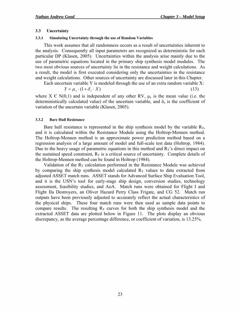
Nathan Andrew Good Chapter 3 – Model Setup
23
3.3 Uncertainty 3.3.1 Simulating Uncertainty through the use of Random Variables
This work assumes that all randomness occurs as a result of uncertainties inherent to the analysis. Consequently all input parameters are recognized as deterministic for each particular DP (Klasen, 2005). Uncertainties within the analysis arise mainly due to the use of parametric equations located in the primary ship synthesis model modules. The two most obvious sources of uncertainty lie in the resistance and weight calculations. As a result, the model is first executed considering only the uncertainties in the resistance and weight calculations. Other sources of uncertainty are discussed later in this Chapter.
Each uncertain variable Y is modeled through the use of an extra random variable X: )1( XY xy ⋅+⋅= δμ (13)
where X Є N(0,1) and is independent of any other RV, μy is the mean value (i.e. the deterministically calculated value) of the uncertain variable, and δx is the coefficient of variation of the uncertain variable (Klasen, 2005). 3.3.2 Bare Hull Resistance
Bare hull resistance is represented in the ship synthesis model by the variable RT, and it is calculated within the Resistance Module using the Holtrop-Mennen method. The Holtrop-Mennen method is an approximate power prediction method based on a regression analysis of a large amount of model and full-scale test data (Holtrop, 1984). Due to the heavy usage of parametric equations in this method and RT’s direct impact on the sustained speed constraint, RT is a critical source of uncertainty. Complete details of the Holtrop-Mennen method can be found in Holtrop (1984).
Validation of the RT calculation performed in the Resistance Module was achieved by comparing the ship synthesis model calculated RT values to data extracted from adjusted ASSET match runs. ASSET stands for Advanced Surface Ship Evaluation Tool, and it is the USN’s tool for early-stage ship design, conversion studies, technology assessment, feasibility studies, and AoA. Match runs were obtained for Flight I and Flight IIa Destroyers, an Oliver Hazard Perry Class Frigate, and CG 52. Match run outputs have been previously adjusted to accurately reflect the actual characteristics of the physical ships. These four match runs were then used as sample data points to compare results. The resulting RT curves for both the ship synthesis model and the extracted ASSET data are plotted below in Figure 11. The plots display an obvious discrepancy, as the average percentage difference, or coefficient of variation, is 13.25%.
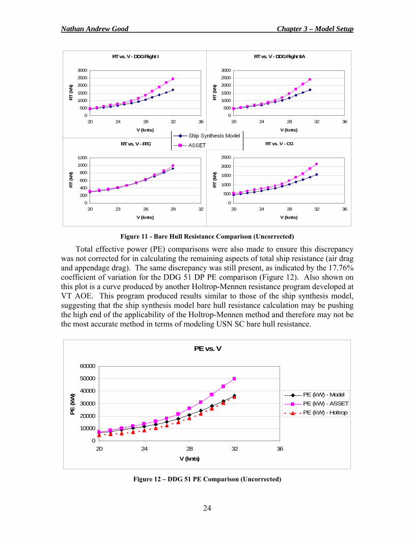
Nathan Andrew Good Chapter 3 – Model Setup
24
Figure 11 - Bare Hull Resistance Comparison (Uncorrected)
Total effective power (PE) comparisons were also made to ensure this discrepancy was not corrected for in calculating the remaining aspects of total ship resistance (air drag and appendage drag). The same discrepancy was still present, as indicated by the 17.76% coefficient of variation for the DDG 51 DP PE comparison (Figure 12). Also shown on this plot is a curve produced by another Holtrop-Mennen resistance program developed at VT AOE. This program produced results similar to those of the ship synthesis model, suggesting that the ship synthesis model bare hull resistance calculation may be pushing the high end of the applicability of the Holtrop-Mennen method and therefore may not be the most accurate method in terms of modeling USN SC bare hull resistance.
PE vs. V
0
10000
20000
30000
40000
50000
60000
20 24 28 32 36
V (knts)
PE
(kW
) PE (kW) - ModelPE (kW) - ASSETPE (kW) - Holtrop
Figure 12 – DDG 51 PE Comparison (Uncorrected)
RT vs. V - DDG Flight I
0
500
1000
1500
2000
2500
3000
20 24 28 32 36
V (knts)
RT
(kN
)
RT vs. V - DDG Flight IIA
0
500
1000
1500
2000
2500
3000
20 24 28 32 36
V (knts)
RT
(kN
)
RT vs. V - FFG
0
200
400
600
800
1000
1200
20 23 26 29 32
V (knts)
RT
(kN
)
RT vs. V - CG
0
500
1000
1500
2000
2500
20 24 28 32 36
V (knts)R
T (k
N)
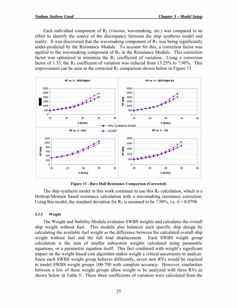
Nathan Andrew Good Chapter 3 – Model Setup
25
Each individual component of RT (viscous, wavemaking, etc.) was compared in an effort to identify the source of the discrepancy between the ship synthesis model and reality. It was discovered that the wavemaking component of RT was being significantly under-predicted by the Resistance Module. To account for this, a correction factor was applied to the wavemaking component of RT in the Resistance Module. This correction factor was optimized to minimize the RT coefficient of variation. Using a correction factor of 1.35, the RT coefficient of variation was reduced from 13.25% to 7.98%. This improvement can be seen in the corrected RT comparison shown below in Figure 13.
Figure 13 - Bare Hull Resistance Comparison (Corrected)
The ship synthesis model in this work continues to use this RT calculation, which is a Holtrop-Mennen based resistance calculation with a wavemaking resistance correction. Using this model, the standard deviation for RT is assumed to be 7.98%, i.e. δ = 0.0798.
3.3.3 Weight
The Weight and Stability Module evaluates SWBS weights and calculates the overall ship weight without fuel. This module also balances each specific ship design by calculating the available fuel weight as the difference between the calculated overall ship weight without fuel and the full load displacement. Each SWBS weight group calculation is the sum of smaller subsystem weights calculated using parametric equations, or a parametric equation itself. This fact combined with weight’s significant impact on the weight-based cost algorithm makes weight a critical uncertainty to analyze. Since each SWBS weight group behaves differently, seven new RVs would be required to model SWBS weight groups 100-700 with complete accuracy. However, similarities between a few of these weight groups allow weight to be analyzed with three RVs as shown below in Table 5. These three coefficients of variation were calculated from the
RT vs. V - DDG Flight I
0
500
1000
1500
2000
2500
3000
20 24 28 32 36
V (knts)
RT vs. V - DDG Flight IIA
0
500
1000
1500
2000
2500
3000
20 24 28 32 36
V (knts)R
T (k
N)
RT vs. V - FFG
0
200
400
600
800
1000
1200
20 23 26 29 32
V (knts)
RT
(kN
)
RT vs. V - CG
0
500
1000
1500
2000
2500
20 24 28 32 36
V (knts)
RT
(kN
)
Nathan Andrew Good Chapter 3 – Model Setup
26
same set of ASSET match runs. Also, it should be noted that in the first model execution involving only two RVs, total lightship weight is summarized with one RV with a coefficient of variation of 10%.
Table 5 - SWBS Weight Group RVs
Random Variable δ Value Description W16 9.94% RV for SWBS 100 & 600 weight groups W235 5.74% RV for SWBS 200, 300, & 500 weight groups W47 9.65% RV for SWBS 400 & 700 weight groups
3.3.4 Other Sources of Uncertainty
Although the two most significant sources of uncertainty are bare hull resistance and weight, there are still other critical sources of uncertainty embedded within the ship synthesis model. The most important sources of uncertainty are those that have a direct impact on the CTOC and OMOE objectives as well as the nine SC design constraints. The largest source of uncertainty within the Cost Module is weight, and the OMOE calculation is based on data-based discrete DVs that are considered deterministic in this analysis. Therefore, a handful of parameters that directly affect the nine design constraints were identified. These other sources of uncertainty are identified below in Table 6. Coefficients of variation were calculated based on ASSET match runs where data was available or assumed to be 10%.
Table 6 - Other Sources of Uncertainty
Random Variable δ Value Description Atr 10.00% RV for total required area E 10.00% RV for endurance range
KG 3.65% RV for KG value KWmflm 13.20% RV for maximum functional load with margins
3.4 Optimization Algorithm
The SC multi-disciplinary ship synthesis model is optimized using a Genetic Algorithm (GA). A GA is an optimization technique based on natural occurring systems used to represent synthetic systems. These algorithms use evolutionary processes such as reproduction, crossover, and mutation based on Darwin’s “survival of the fittest” principle to improve upon an initial population of balanced designs. Crossover involves swapping genes (design variables) between parent designs to produce a new child design, while mutation is modification of the genes of an individual parent design to produce a new child design. GAs are very robust relative to other optimization techniques, and they are particularly advantageous in optimizing models with discontinuous functions or data-based discrete DVs. An optimization technique is considered robust if it is able to effectively and efficiently explore the design space, i.e. it consistently locates the global optimum using minimal computational effort (Brown and Thomas, 1998).
Multi-Objective Genetic Optimization (MOGO) is performed in MC using the Darwin Optimization plug-in, which is described in greater detail in Section 3.4.1. A flow chart of the MOGO process used in this work is shown in Figure 14. The optimizer
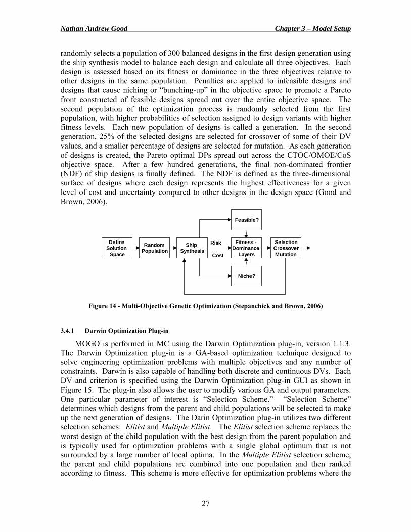
Nathan Andrew Good Chapter 3 – Model Setup
27
randomly selects a population of 300 balanced designs in the first design generation using the ship synthesis model to balance each design and calculate all three objectives. Each design is assessed based on its fitness or dominance in the three objectives relative to other designs in the same population. Penalties are applied to infeasible designs and designs that cause niching or “bunching-up” in the objective space to promote a Pareto front constructed of feasible designs spread out over the entire objective space. The second population of the optimization process is randomly selected from the first population, with higher probabilities of selection assigned to design variants with higher fitness levels. Each new population of designs is called a generation. In the second generation, 25% of the selected designs are selected for crossover of some of their DV values, and a smaller percentage of designs are selected for mutation. As each generation of designs is created, the Pareto optimal DPs spread out across the CTOC/OMOE/CoS objective space. After a few hundred generations, the final non-dominated frontier (NDF) of ship designs is finally defined. The NDF is defined as the three-dimensional surface of designs where each design represents the highest effectiveness for a given level of cost and uncertainty compared to other designs in the design space (Good and Brown, 2006).
DefineSolution
Space
RandomPopulation
ShipSynthesis
Feasible?
Niche?
Fitness -Dominance
Layers
SelectionCrossoverMutation
Risk
Cost
Figure 14 - Multi-Objective Genetic Optimization (Stepanchick and Brown, 2006)
3.4.1 Darwin Optimization Plug-in
MOGO is performed in MC using the Darwin Optimization plug-in, version 1.1.3. The Darwin Optimization plug-in is a GA-based optimization technique designed to solve engineering optimization problems with multiple objectives and any number of constraints. Darwin is also capable of handling both discrete and continuous DVs. Each DV and criterion is specified using the Darwin Optimization plug-in GUI as shown in Figure 15. The plug-in also allows the user to modify various GA and output parameters. One particular parameter of interest is “Selection Scheme.” “Selection Scheme” determines which designs from the parent and child populations will be selected to make up the next generation of designs. The Darin Optimization plug-in utilizes two different selection schemes: Elitist and Multiple Elitist. The Elitist selection scheme replaces the worst design of the child population with the best design from the parent population and is typically used for optimization problems with a single global optimum that is not surrounded by a large number of local optima. In the Multiple Elitist selection scheme, the parent and child populations are combined into one population and then ranked according to fitness. This scheme is more effective for optimization problems where the
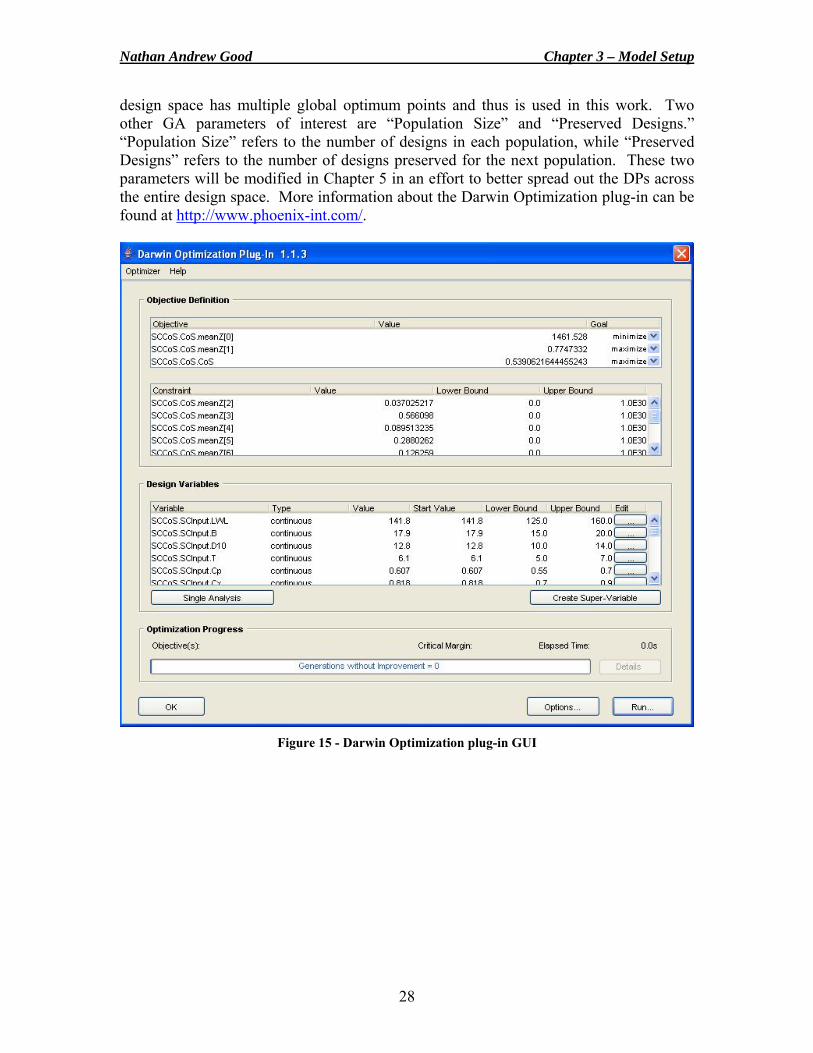
Nathan Andrew Good Chapter 3 – Model Setup
28
design space has multiple global optimum points and thus is used in this work. Two other GA parameters of interest are “Population Size” and “Preserved Designs.” “Population Size” refers to the number of designs in each population, while “Preserved Designs” refers to the number of designs preserved for the next population. These two parameters will be modified in Chapter 5 in an effort to better spread out the DPs across the entire design space. More information about the Darwin Optimization plug-in can be found at http://www.phoenix-int.com/.
Figure 15 - Darwin Optimization plug-in GUI
29
4 Model Execution
The two most critical sources of uncertainty in the multi-disciplinary ship synthesis model described in the preceding section lie in the resistance and weight calculations. As a result, the CoS calculation is first implemented and incorporated into the optimization process of the ship synthesis model by considering only uncertainties in the resistance and weight calculations. However, before the initial model execution, an examination of the model response is performed. 4.1 Model Response Examination
As mentioned earlier, the usage of the suggested CoS calculation calls for close to linear responses locally within the design space and/or concentration of responses around the mean performance value. In regions in close vicinity to a DP, there is a high probability of a continuous, well-behaved, linear response, even though no response function can be expected to behave this way throughout the entire design space of a complex multi-disciplinary ship synthesis model. If responses exhibit continuous, near linear behavior and have low variance, the CoS calculation suggested in this work should be applicable. To examine criteria response behavior, Klasen selected a few deterministically feasible DPs at random and evaluated them via short sample MCS calculations of 100,000 system evaluations each (Klasen, 2005). Although Klasen used a previous version of the ship synthesis model, the RV relationships and general criteria response behavior have not changed.
All evaluated DPs yielded an almost linear response over the ranges of interest for the CTOC objective as well as the Ata, Cgmbmin, and Cgmbmax constraint error values (See Table 4). Exceptions included the Vs and E constraint error values, which were both non-linear but continuous, as well as the OMOE objective, which was non-linear and discontinuous. The Ada, KWg, and D10 constraint error values are not a function of the RVs. The Brake Propulsion Power at Endurance Speed constraint error value (Pbpengend) was not included in Klasen’s model, but its criteria response behavior was found to be almost linear over the range of interest. Some of Klasen’s criteria response surfaces for the DDG 51 DP are presented in Figure 16. These include the CTOC (Figure 16.1) and OMOE (Figure 16.2) objectives, and the endurance range (Figure 16.3) and sustained speed (Figure 16.4) constraint error values plotted as a function of bare hull resistance (RT) and total weight (WT). In these figures, the mesh size is σ for both bare hull resistance and total weight. A higher probability of occurrence is represented by the darker region of the response surfaces (Klasen, 2005).
The relatively well-behaved response surfaces of the CTOC objective and the constraints indicate that the first order Taylor series expansion of MV should be sufficient to approximate the response functions accurately in local regions of any DP. This means that the CoS calculation suggested in this work should be applicable.
As mentioned earlier, the OMOE objective response surface was both non-linear and discontinuous. Although its surface appears to have the same general form throughout the entire design space, there are differences in plateau shape, size, and position for each individual DP. This means that a first order Taylor series expansion will have significant problems approximating an accurate response surface to this shape (Klasen, 2005).
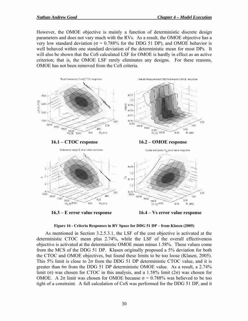
Nathan Andrew Good Chapter 4 – Model Execution
30
However, the OMOE objective is mainly a function of deterministic discrete design parameters and does not vary much with the RVs. As a result, the OMOE objective has a very low standard deviation (σ = 0.788% for the DDG 51 DP), and OMOE behavior is well behaved within one standard deviation of the deterministic mean for most DPs. It will also be shown that the CoS calculated LSF for OMOE is hardly in effect as an active criterion; that is, the OMOE LSF rarely eliminates any designs. For these reasons, OMOE has not been removed from the CoS criteria.
16.1 – CTOC response 16.2 – OMOE response
16.3 – E error value response 16.4 – Vs error value response
Figure 16 - Criteria Responses in RV Space for DDG 51 DP – from Klasen (2005)
As mentioned in Section 3.2.5.3.1, the LSF of the cost objective is activated at the deterministic CTOC mean plus 2.74%, while the LSF of the overall effectiveness objective is activated at the deterministic OMOE mean minus 1.58%. These values come from the MCS of the DDG 51 DP. Klasen originally proposed a 5% deviation for both the CTOC and OMOE objectives, but found these limits to be too loose (Klasen, 2005). This 5% limit is close to 2σ from the DDG 51 DP deterministic CTOC value, and it is greater than 6σ from the DDG 51 DP deterministic OMOE value. As a result, a 2.74% limit (σ) was chosen for CTOC in this analysis, and a 1.58% limit (2σ) was chosen for OMOE. A 2σ limit was chosen for OMOE because σ = 0.788% was believed to be too tight of a constraint. A full calculation of CoS was performed for the DDG 51 DP, and it
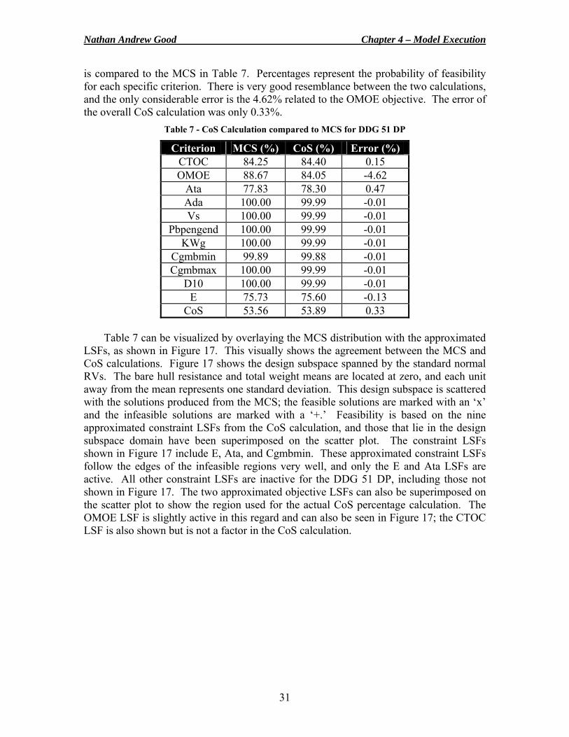
Nathan Andrew Good Chapter 4 – Model Execution
31
is compared to the MCS in Table 7. Percentages represent the probability of feasibility for each specific criterion. There is very good resemblance between the two calculations, and the only considerable error is the 4.62% related to the OMOE objective. The error of the overall CoS calculation was only 0.33%.
Table 7 - CoS Calculation compared to MCS for DDG 51 DP
Criterion MCS (%) CoS (%) Error (%) CTOC 84.25 84.40 0.15 OMOE 88.67 84.05 -4.62
Ata 77.83 78.30 0.47 Ada 100.00 99.99 -0.01 Vs 100.00 99.99 -0.01
Pbpengend 100.00 99.99 -0.01 KWg 100.00 99.99 -0.01
Cgmbmin 99.89 99.88 -0.01 Cgmbmax 100.00 99.99 -0.01
D10 100.00 99.99 -0.01 E 75.73 75.60 -0.13
CoS 53.56 53.89 0.33 Table 7 can be visualized by overlaying the MCS distribution with the approximated
LSFs, as shown in Figure 17. This visually shows the agreement between the MCS and CoS calculations. Figure 17 shows the design subspace spanned by the standard normal RVs. The bare hull resistance and total weight means are located at zero, and each unit away from the mean represents one standard deviation. This design subspace is scattered with the solutions produced from the MCS; the feasible solutions are marked with an ‘x’ and the infeasible solutions are marked with a ‘+.’ Feasibility is based on the nine approximated constraint LSFs from the CoS calculation, and those that lie in the design subspace domain have been superimposed on the scatter plot. The constraint LSFs shown in Figure 17 include E, Ata, and Cgmbmin. These approximated constraint LSFs follow the edges of the infeasible regions very well, and only the E and Ata LSFs are active. All other constraint LSFs are inactive for the DDG 51 DP, including those not shown in Figure 17. The two approximated objective LSFs can also be superimposed on the scatter plot to show the region used for the actual CoS percentage calculation. The OMOE LSF is slightly active in this regard and can also be seen in Figure 17; the CTOC LSF is also shown but is not a factor in the CoS calculation.
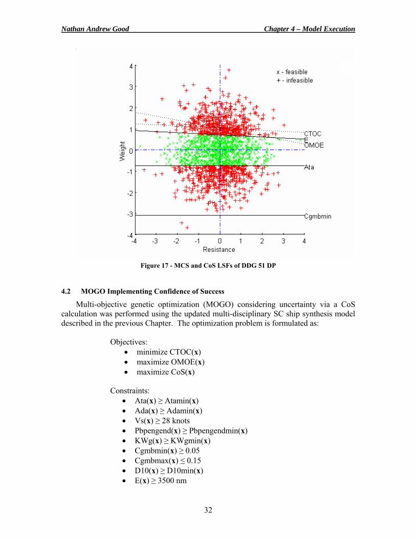
Nathan Andrew Good Chapter 4 – Model Execution
32
Figure 17 - MCS and CoS LSFs of DDG 51 DP
4.2 MOGO Implementing Confidence of Success
Multi-objective genetic optimization (MOGO) considering uncertainty via a CoS calculation was performed using the updated multi-disciplinary SC ship synthesis model described in the previous Chapter. The optimization problem is formulated as: Objectives:
• minimize CTOC(x) • maximize OMOE(x) • maximize CoS(x)
Constraints:
• Ata(x) ≥ Atamin(x) • Ada(x) ≥ Adamin(x) • Vs(x) ≥ 28 knots • Pbpengend(x) ≥ Pbpengendmin(x) • KWg(x) ≥ KWgmin(x) • Cgmbmin(x) ≥ 0.05 • Cgmbmax(x) ≤ 0.15 • D10(x) ≥ D10min(x) • E(x) ≥ 3500 nm
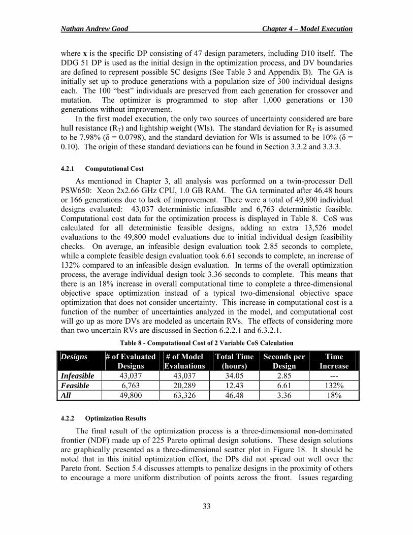
Nathan Andrew Good Chapter 4 – Model Execution
33
where x is the specific DP consisting of 47 design parameters, including D10 itself. The DDG 51 DP is used as the initial design in the optimization process, and DV boundaries are defined to represent possible SC designs (See Table 3 and Appendix B). The GA is initially set up to produce generations with a population size of 300 individual designs each. The 100 “best” individuals are preserved from each generation for crossover and mutation. The optimizer is programmed to stop after 1,000 generations or 130 generations without improvement.
In the first model execution, the only two sources of uncertainty considered are bare hull resistance (RT) and lightship weight (Wls). The standard deviation for RT is assumed to be 7.98% (δ = 0.0798), and the standard deviation for Wls is assumed to be 10% (δ = 0.10). The origin of these standard deviations can be found in Section 3.3.2 and 3.3.3. 4.2.1 Computational Cost
As mentioned in Chapter 3, all analysis was performed on a twin-processor Dell PSW650: Xeon 2x2.66 GHz CPU, 1.0 GB RAM. The GA terminated after 46.48 hours or 166 generations due to lack of improvement. There were a total of 49,800 individual designs evaluated: 43,037 deterministic infeasible and 6,763 deterministic feasible. Computational cost data for the optimization process is displayed in Table 8. CoS was calculated for all deterministic feasible designs, adding an extra 13,526 model evaluations to the 49,800 model evaluations due to initial individual design feasibility checks. On average, an infeasible design evaluation took 2.85 seconds to complete, while a complete feasible design evaluation took 6.61 seconds to complete, an increase of 132% compared to an infeasible design evaluation. In terms of the overall optimization process, the average individual design took 3.36 seconds to complete. This means that there is an 18% increase in overall computational time to complete a three-dimensional objective space optimization instead of a typical two-dimensional objective space optimization that does not consider uncertainty. This increase in computational cost is a function of the number of uncertainties analyzed in the model, and computational cost will go up as more DVs are modeled as uncertain RVs. The effects of considering more than two uncertain RVs are discussed in Section 6.2.2.1 and 6.3.2.1.
Table 8 - Computational Cost of 2 Variable CoS Calculation
Designs # of Evaluated Designs
# of Model Evaluations
Total Time (hours)
Seconds per Design
Time Increase
Infeasible 43,037 43,037 34.05 2.85 --- Feasible 6,763 20,289 12.43 6.61 132% All 49,800 63,326 46.48 3.36 18% 4.2.2 Optimization Results
The final result of the optimization process is a three-dimensional non-dominated frontier (NDF) made up of 225 Pareto optimal design solutions. These design solutions are graphically presented as a three-dimensional scatter plot in Figure 18. It should be noted that in this initial optimization effort, the DPs did not spread out well over the Pareto front. Section 5.4 discusses attempts to penalize designs in the proximity of others to encourage a more uniform distribution of points across the front. Issues regarding
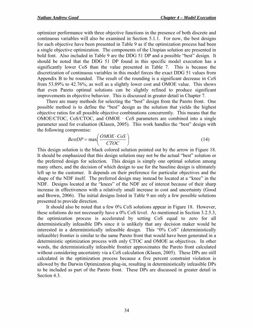
Nathan Andrew Good Chapter 4 – Model Execution
34
optimizer performance with three objective functions in the presence of both discrete and continuous variables will also be examined in Section 5.1.1. For now, the best designs for each objective have been presented in Table 9 as if the optimization process had been a single objective optimization. The components of the Utopian solution are presented in bold font. Also included in Table 9 are the DDG 51 DP and a possible “best” design. It should be noted that the DDG 51 DP found in this specific model execution has a significantly lower CoS than the value presented in Table 7. This is because the discretization of continuous variables in this model forces the exact DDG 51 values from Appendix B to be rounded. The result of the rounding is a significant decrease in CoS from 53.89% to 42.76%, as well as a slightly lower cost and OMOE value. This shows that even Pareto optimal solutions can be slightly refined to produce significant improvements in objective behavior. This is discussed in greater detail in Chapter 7.
There are many methods for selecting the “best” design from the Pareto front. One possible method is to define the “best” design as the solution that yields the highest objective ratios for all possible objective combinations concurrently. This means that the OMOE/CTOC, CoS/CTOC, and OMOE · CoS parameters are combined into a single parameter used for evaluation (Klasen, 2005). This work handles the “best” design with the following compromise:
⎟⎠⎞
⎜⎝⎛ ⋅
=CTOC
CoSOMOEBestDP max (14)
This design solution is the black colored solution pointed out by the arrow in Figure 18. It should be emphasized that this design solution may not be the actual “best” solution or the preferred design for selection. This design is simply one optimal solution among many others, and the decision of which design to use for the baseline design is ultimately left up to the customer. It depends on their preference for particular objectives and the shape of the NDF itself. The preferred design may instead be located at a “knee” in the NDF. Designs located at the “knees” of the NDF are of interest because of their sharp increase in effectiveness with a relatively small increase in cost and uncertainty (Good and Brown, 2006). The initial designs listed in Table 9 are only a few possible solutions presented to provide direction.
It should also be noted that a few 0% CoS solutions appear in Figure 18. However, these solutions do not necessarily have a 0% CoS level. As mentioned in Section 3.2.5.3, the optimization process is accelerated by setting CoS equal to zero for all deterministically infeasible DPs since it is unlikely that any decision maker would be interested in a deterministically infeasible design. This “0% CoS” (deterministically infeasible) frontier is similar to the same Pareto front that would have been generated in a deterministic optimization process with only CTOC and OMOE as objectives. In other words, the deterministically infeasible frontier approximates the Pareto front calculated without considering uncertainty via a CoS calculation (Klasen, 2005). These DPs are still calculated in the optimization process because a five percent constraint violation is allowed by the Darwin Optimization plug-in, resulting in deterministically infeasible DPs to be included as part of the Pareto front. These DPs are discussed in greater detail in Section 4.3.
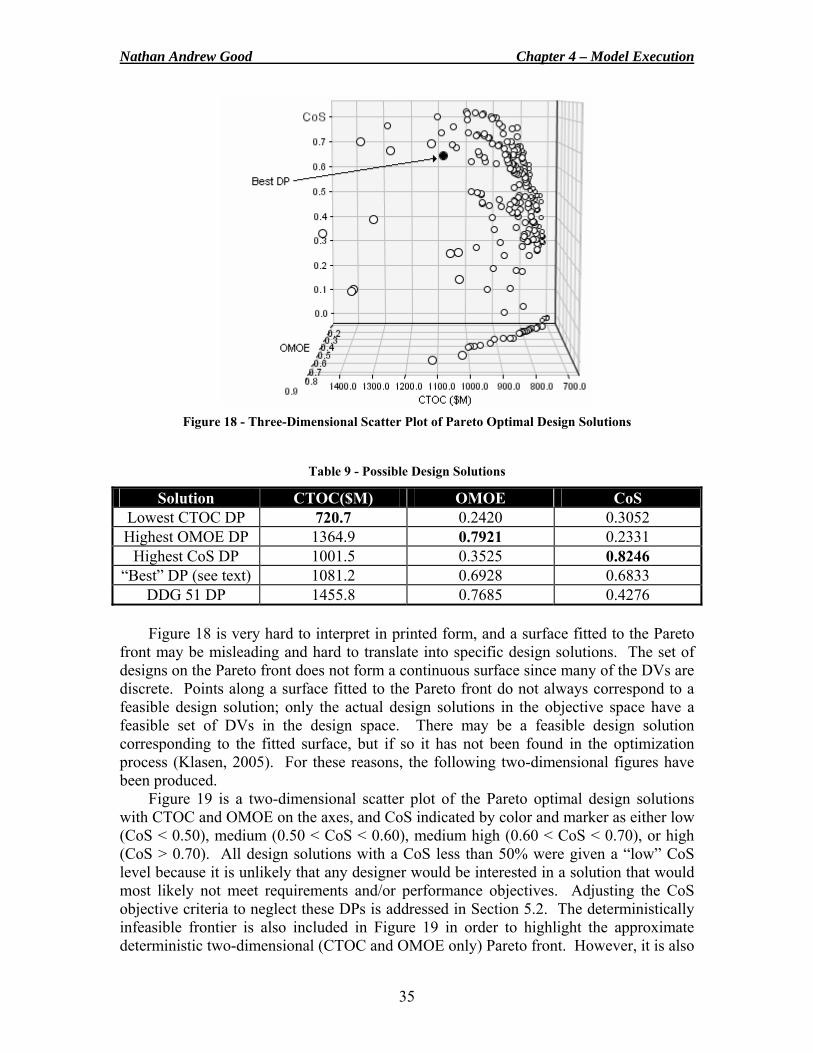
Nathan Andrew Good Chapter 4 – Model Execution
35
Figure 18 - Three-Dimensional Scatter Plot of Pareto Optimal Design Solutions
Table 9 - Possible Design Solutions
Solution CTOC($M) OMOE CoS Lowest CTOC DP 720.7 0.2420 0.3052 Highest OMOE DP 1364.9 0.7921 0.2331
Highest CoS DP 1001.5 0.3525 0.8246 “Best” DP (see text) 1081.2 0.6928 0.6833
DDG 51 DP 1455.8 0.7685 0.4276
Figure 18 is very hard to interpret in printed form, and a surface fitted to the Pareto front may be misleading and hard to translate into specific design solutions. The set of designs on the Pareto front does not form a continuous surface since many of the DVs are discrete. Points along a surface fitted to the Pareto front do not always correspond to a feasible design solution; only the actual design solutions in the objective space have a feasible set of DVs in the design space. There may be a feasible design solution corresponding to the fitted surface, but if so it has not been found in the optimization process (Klasen, 2005). For these reasons, the following two-dimensional figures have been produced.
Figure 19 is a two-dimensional scatter plot of the Pareto optimal design solutions with CTOC and OMOE on the axes, and CoS indicated by color and marker as either low (CoS < 0.50), medium (0.50 < CoS < 0.60), medium high (0.60 < CoS < 0.70), or high (CoS > 0.70). All design solutions with a CoS less than 50% were given a “low” CoS level because it is unlikely that any designer would be interested in a solution that would most likely not meet requirements and/or performance objectives. Adjusting the CoS objective criteria to neglect these DPs is addressed in Section 5.2. The deterministically infeasible frontier is also included in Figure 19 in order to highlight the approximate deterministic two-dimensional (CTOC and OMOE only) Pareto front. However, it is also
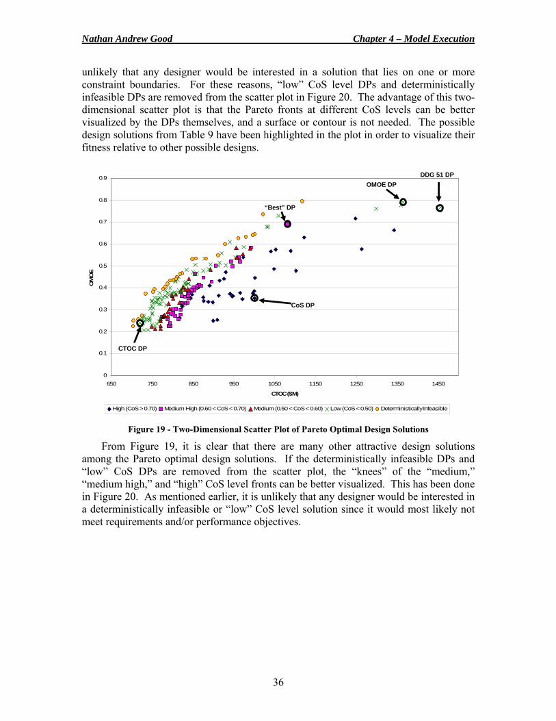
Nathan Andrew Good Chapter 4 – Model Execution
36
unlikely that any designer would be interested in a solution that lies on one or more constraint boundaries. For these reasons, “low” CoS level DPs and deterministically infeasible DPs are removed from the scatter plot in Figure 20. The advantage of this two-dimensional scatter plot is that the Pareto fronts at different CoS levels can be better visualized by the DPs themselves, and a surface or contour is not needed. The possible design solutions from Table 9 have been highlighted in the plot in order to visualize their fitness relative to other possible designs.
Figure 19 - Two-Dimensional Scatter Plot of Pareto Optimal Design Solutions
From Figure 19, it is clear that there are many other attractive design solutions among the Pareto optimal design solutions. If the deterministically infeasible DPs and “low” CoS DPs are removed from the scatter plot, the “knees” of the “medium,” “medium high,” and “high” CoS level fronts can be better visualized. This has been done in Figure 20. As mentioned earlier, it is unlikely that any designer would be interested in a deterministically infeasible or “low” CoS level solution since it would most likely not meet requirements and/or performance objectives.
0
0.1
0.2
0.3
0.4
0.5
0.6
0.7
0.8
0.9
650 750 850 950 1050 1150 1250 1350 1450
CTOC ($M)
OM
OE
High (CoS > 0.70) Medium High (0.60 < CoS < 0.70) Medium (0.50 < CoS < 0.60) Low (CoS < 0.50) Deterministically Infeasible
DDG 51 DPOMOE DP
“Best” DP
CoS DP
CTOC DP
Nathan Andrew Good Chapter 4 – Model Execution
37
Figure 20 - 2-D Scatter Plot of Pareto Front (Det. Infeasible and “Low” CoS DPs Removed)
Figure 20 shows the “knees” of the remaining CoS levels and the other attractive designs. It should be noted that both “Knee” 3 and “Knee” 4 correspond to the “medium” CoS level. It should also be noted that the lowest CTOC DP, highest OMOE DP, and DDG 51 DP have been removed since they had a CoS less than 50%. The objectives of the four “knees” are shown in Table 10.
Table 10 – Other Attractive Design Solutions
Solution CTOC($M) OMOE CoS “Knee” 1 DP 973.2 0.5411 0.7437 “Knee” 2 DP 856.1 0.4648 0.6199 “Knee” 3 DP 840.1 0.4418 0.5447 “Knee” 4 DP 956.1 0.5834 0.5061
Of the 225 Pareto optimal design solutions, the highest CoS DP, “best” DP, and four
“knees” appear to be the most attractive designs. The DDG 51 DP should also be included as an attractive design since it has been proven feasible in the real world. It is also close to the OMOE objective extreme due to its emphasis on combat systems. Since the DDG 51 DP lies on this particular Pareto front, there are no designs from this optimization run that outperform the DDG 51 DP in all objectives concurrently, i.e. there are no other designs that are cheaper, more effective, and less uncertain. However, it will be shown that the DDG 51 DP is not Pareto optimal in future optimization runs where DPs are found that exhibit performance increases in all three objectives concurrently. Also, the other attractive designs mentioned may be “better” solutions since they offer significant cost savings and an increase in CoS.
0
0.1
0.2
0.3
0.4
0.5
0.6
0.7
0.8
700 800 900 1000 1100 1200 1300 1400
CTOC ($M)
OM
OE
High (CoS > 0.70) Medium High (0.60 < CoS < 0.70) Medium (0.50 < CoS < 0.60)
“Best” DP
CoS DP
“Knee” 1
“Knee” 2
“Knee” 3
“Knee” 4
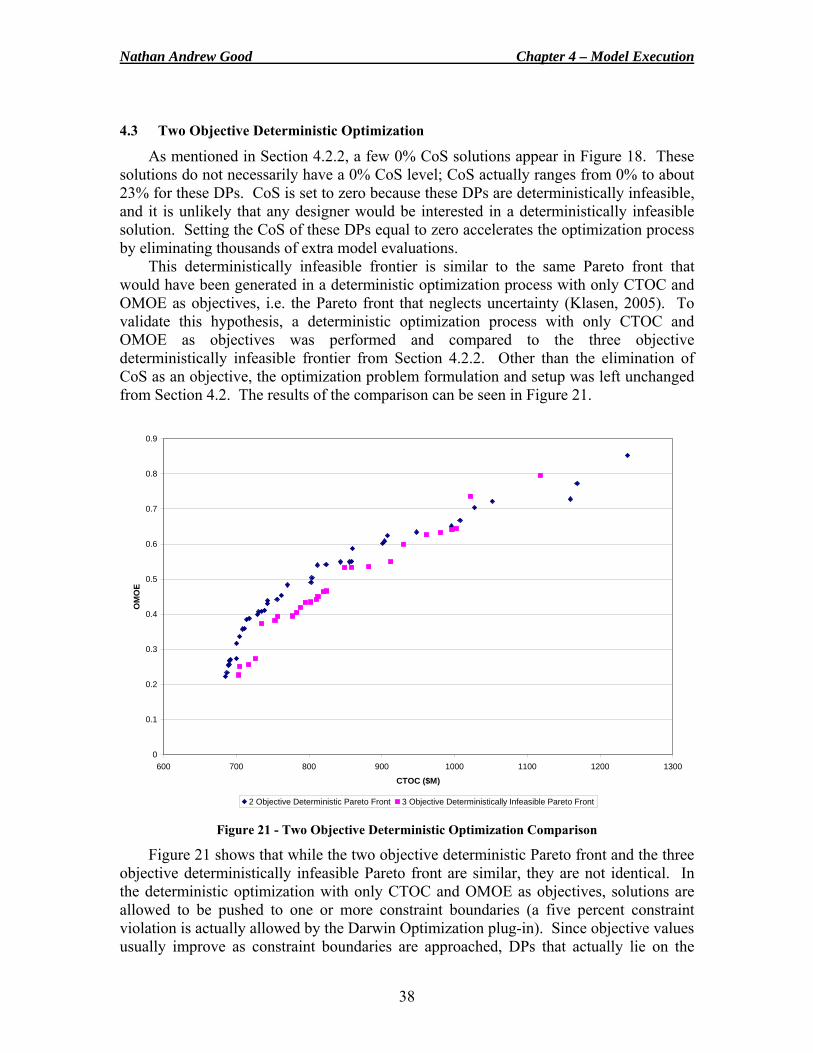
Nathan Andrew Good Chapter 4 – Model Execution
38
4.3 Two Objective Deterministic Optimization
As mentioned in Section 4.2.2, a few 0% CoS solutions appear in Figure 18. These solutions do not necessarily have a 0% CoS level; CoS actually ranges from 0% to about 23% for these DPs. CoS is set to zero because these DPs are deterministically infeasible, and it is unlikely that any designer would be interested in a deterministically infeasible solution. Setting the CoS of these DPs equal to zero accelerates the optimization process by eliminating thousands of extra model evaluations.
This deterministically infeasible frontier is similar to the same Pareto front that would have been generated in a deterministic optimization process with only CTOC and OMOE as objectives, i.e. the Pareto front that neglects uncertainty (Klasen, 2005). To validate this hypothesis, a deterministic optimization process with only CTOC and OMOE as objectives was performed and compared to the three objective deterministically infeasible frontier from Section 4.2.2. Other than the elimination of CoS as an objective, the optimization problem formulation and setup was left unchanged from Section 4.2. The results of the comparison can be seen in Figure 21.
0
0.1
0.2
0.3
0.4
0.5
0.6
0.7
0.8
0.9
600 700 800 900 1000 1100 1200 1300
CTOC ($M)
OM
OE
2 Objective Deterministic Pareto Front 3 Objective Deterministically Infeasible Pareto Front Figure 21 - Two Objective Deterministic Optimization Comparison
Figure 21 shows that while the two objective deterministic Pareto front and the three objective deterministically infeasible Pareto front are similar, they are not identical. In the deterministic optimization with only CTOC and OMOE as objectives, solutions are allowed to be pushed to one or more constraint boundaries (a five percent constraint violation is actually allowed by the Darwin Optimization plug-in). Since objective values usually improve as constraint boundaries are approached, DPs that actually lie on the
Nathan Andrew Good Chapter 4 – Model Execution
39
constraint boundaries are more attractive in a two objective deterministic optimization process. Essentially, the entire population tends to migrate towards constraint boundaries because the constraint boundaries represent the best you can do in terms of only CTOC and OMOE. In fact, of the 41 Pareto optimal design solutions from the two objective deterministic Pareto front, only two DPs are deterministically feasible. These two DPs have been presented in bold font in Table 11.
In contrast, in a three objective optimization process that considers uncertainty via a CoS calculation, deterministically infeasible design solutions are less attractive because they have been assigned a CoS value of 0% and because maximizing CoS has been selected as an objective. As a result, a three objective optimization process will only tag an approximation of the two objective deterministic Pareto front, and it will then penalize these designs further to encourage more attractive DPs that perform well in all three objectives. Consequently, the deterministically infeasible frontier from the three objective optimization process that considers uncertainty is just a slight-under approximation of the two objective deterministic Pareto front, as shown in Figure 21.
Table 11 displays the actual CoS values for the DPS from the two objective deterministic Pareto front. As mentioned earlier, 39 of the 41 solutions were deterministically infeasible, and 12 of these 39 deterministically infeasible solutions actually had a CoS of 0% as calculated by the procedure used in this work. Several of the other solutions had very low CoS levels, ranging only up to 23.19%. This shows that while a deterministic optimization process may yield the best objective values, it may also yield the highest uncertainty levels as well. This is further evidence that any optimization process must be performed with a constraint on uncertainty, or uncertainty must be treated as a third objective. By treating CoS as an objective, the optimizer will search for more reliable and robust designs. Otherwise there is virtually no chance of achieving results that are reliable and robust in addition to being effective.
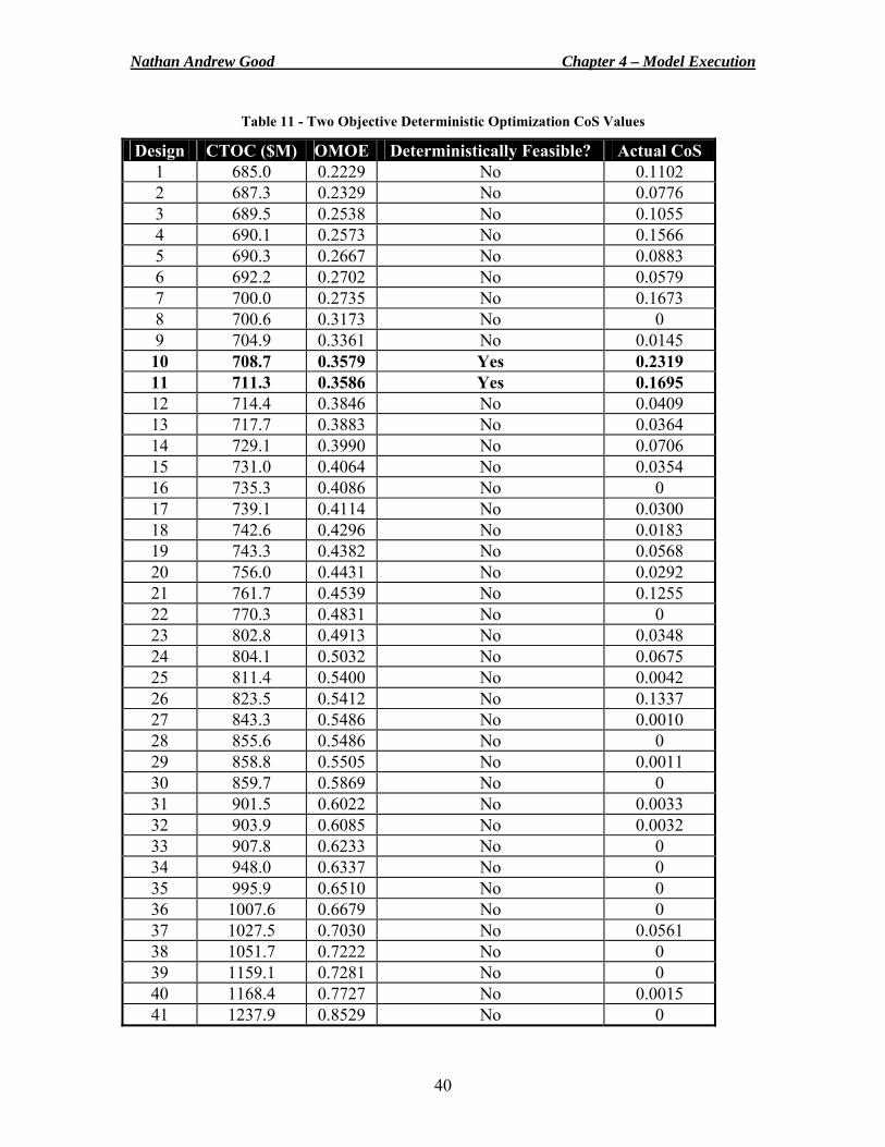
Nathan Andrew Good Chapter 4 – Model Execution
40
Table 11 - Two Objective Deterministic Optimization CoS Values
Design CTOC ($M) OMOE Deterministically Feasible? Actual CoS 1 685.0 0.2229 No 0.1102 2 687.3 0.2329 No 0.0776 3 689.5 0.2538 No 0.1055 4 690.1 0.2573 No 0.1566 5 690.3 0.2667 No 0.0883 6 692.2 0.2702 No 0.0579 7 700.0 0.2735 No 0.1673 8 700.6 0.3173 No 0 9 704.9 0.3361 No 0.0145 10 708.7 0.3579 Yes 0.2319 11 711.3 0.3586 Yes 0.1695 12 714.4 0.3846 No 0.0409 13 717.7 0.3883 No 0.0364 14 729.1 0.3990 No 0.0706 15 731.0 0.4064 No 0.0354 16 735.3 0.4086 No 0 17 739.1 0.4114 No 0.0300 18 742.6 0.4296 No 0.0183 19 743.3 0.4382 No 0.0568 20 756.0 0.4431 No 0.0292 21 761.7 0.4539 No 0.1255 22 770.3 0.4831 No 0 23 802.8 0.4913 No 0.0348 24 804.1 0.5032 No 0.0675 25 811.4 0.5400 No 0.0042 26 823.5 0.5412 No 0.1337 27 843.3 0.5486 No 0.0010 28 855.6 0.5486 No 0 29 858.8 0.5505 No 0.0011 30 859.7 0.5869 No 0 31 901.5 0.6022 No 0.0033 32 903.9 0.6085 No 0.0032 33 907.8 0.6233 No 0 34 948.0 0.6337 No 0 35 995.9 0.6510 No 0 36 1007.6 0.6679 No 0 37 1027.5 0.7030 No 0.0561 38 1051.7 0.7222 No 0 39 1159.1 0.7281 No 0 40 1168.4 0.7727 No 0.0015 41 1237.9 0.8529 No 0
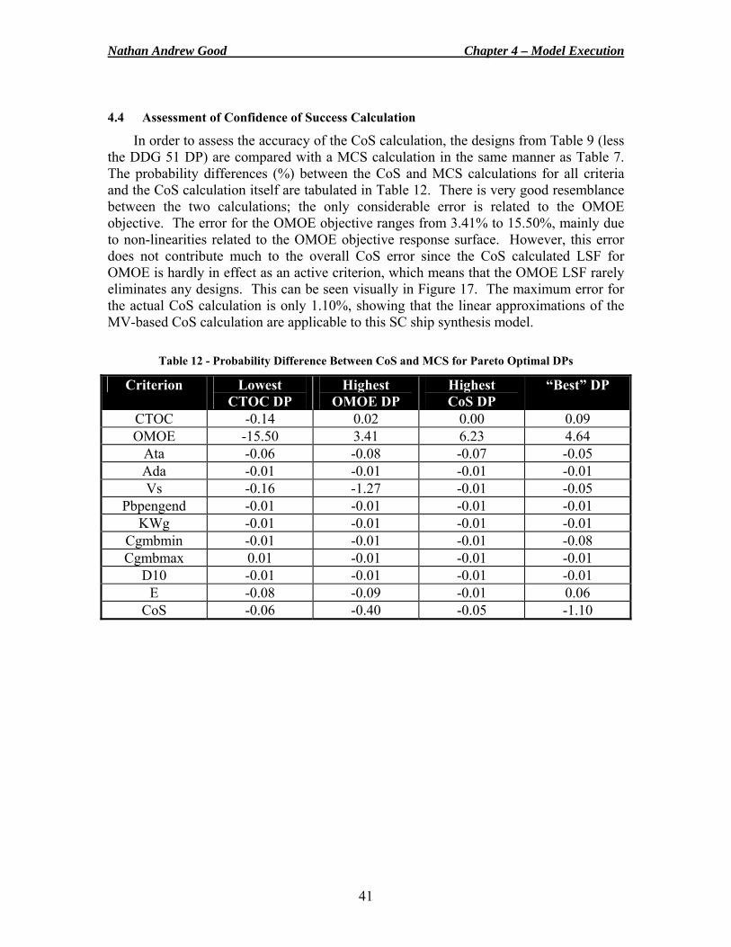
Nathan Andrew Good Chapter 4 – Model Execution
41
4.4 Assessment of Confidence of Success Calculation
In order to assess the accuracy of the CoS calculation, the designs from Table 9 (less the DDG 51 DP) are compared with a MCS calculation in the same manner as Table 7. The probability differences (%) between the CoS and MCS calculations for all criteria and the CoS calculation itself are tabulated in Table 12. There is very good resemblance between the two calculations; the only considerable error is related to the OMOE objective. The error for the OMOE objective ranges from 3.41% to 15.50%, mainly due to non-linearities related to the OMOE objective response surface. However, this error does not contribute much to the overall CoS error since the CoS calculated LSF for OMOE is hardly in effect as an active criterion, which means that the OMOE LSF rarely eliminates any designs. This can be seen visually in Figure 17. The maximum error for the actual CoS calculation is only 1.10%, showing that the linear approximations of the MV-based CoS calculation are applicable to this SC ship synthesis model.
Table 12 - Probability Difference Between CoS and MCS for Pareto Optimal DPs
Criterion Lowest CTOC DP
Highest OMOE DP
Highest CoS DP
“Best” DP
CTOC -0.14 0.02 0.00 0.09 OMOE -15.50 3.41 6.23 4.64
Ata -0.06 -0.08 -0.07 -0.05 Ada -0.01 -0.01 -0.01 -0.01 Vs -0.16 -1.27 -0.01 -0.05
Pbpengend -0.01 -0.01 -0.01 -0.01 KWg -0.01 -0.01 -0.01 -0.01
Cgmbmin -0.01 -0.01 -0.01 -0.08 Cgmbmax 0.01 -0.01 -0.01 -0.01
D10 -0.01 -0.01 -0.01 -0.01 E -0.08 -0.09 -0.01 0.06
CoS -0.06 -0.40 -0.05 -1.10
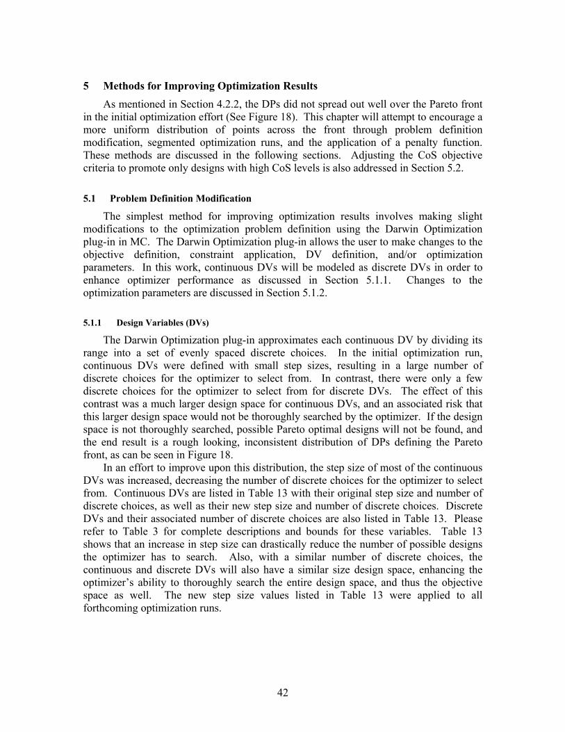
42
5 Methods for Improving Optimization Results
As mentioned in Section 4.2.2, the DPs did not spread out well over the Pareto front in the initial optimization effort (See Figure 18). This chapter will attempt to encourage a more uniform distribution of points across the front through problem definition modification, segmented optimization runs, and the application of a penalty function. These methods are discussed in the following sections. Adjusting the CoS objective criteria to promote only designs with high CoS levels is also addressed in Section 5.2. 5.1 Problem Definition Modification
The simplest method for improving optimization results involves making slight modifications to the optimization problem definition using the Darwin Optimization plug-in in MC. The Darwin Optimization plug-in allows the user to make changes to the objective definition, constraint application, DV definition, and/or optimization parameters. In this work, continuous DVs will be modeled as discrete DVs in order to enhance optimizer performance as discussed in Section 5.1.1. Changes to the optimization parameters are discussed in Section 5.1.2.
5.1.1 Design Variables (DVs)
The Darwin Optimization plug-in approximates each continuous DV by dividing its range into a set of evenly spaced discrete choices. In the initial optimization run, continuous DVs were defined with small step sizes, resulting in a large number of discrete choices for the optimizer to select from. In contrast, there were only a few discrete choices for the optimizer to select from for discrete DVs. The effect of this contrast was a much larger design space for continuous DVs, and an associated risk that this larger design space would not be thoroughly searched by the optimizer. If the design space is not thoroughly searched, possible Pareto optimal designs will not be found, and the end result is a rough looking, inconsistent distribution of DPs defining the Pareto front, as can be seen in Figure 18.
In an effort to improve upon this distribution, the step size of most of the continuous DVs was increased, decreasing the number of discrete choices for the optimizer to select from. Continuous DVs are listed in Table 13 with their original step size and number of discrete choices, as well as their new step size and number of discrete choices. Discrete DVs and their associated number of discrete choices are also listed in Table 13. Please refer to Table 3 for complete descriptions and bounds for these variables. Table 13 shows that an increase in step size can drastically reduce the number of possible designs the optimizer has to search. Also, with a similar number of discrete choices, the continuous and discrete DVs will also have a similar size design space, enhancing the optimizer’s ability to thoroughly search the entire design space, and thus the objective space as well. The new step size values listed in Table 13 were applied to all forthcoming optimization runs.
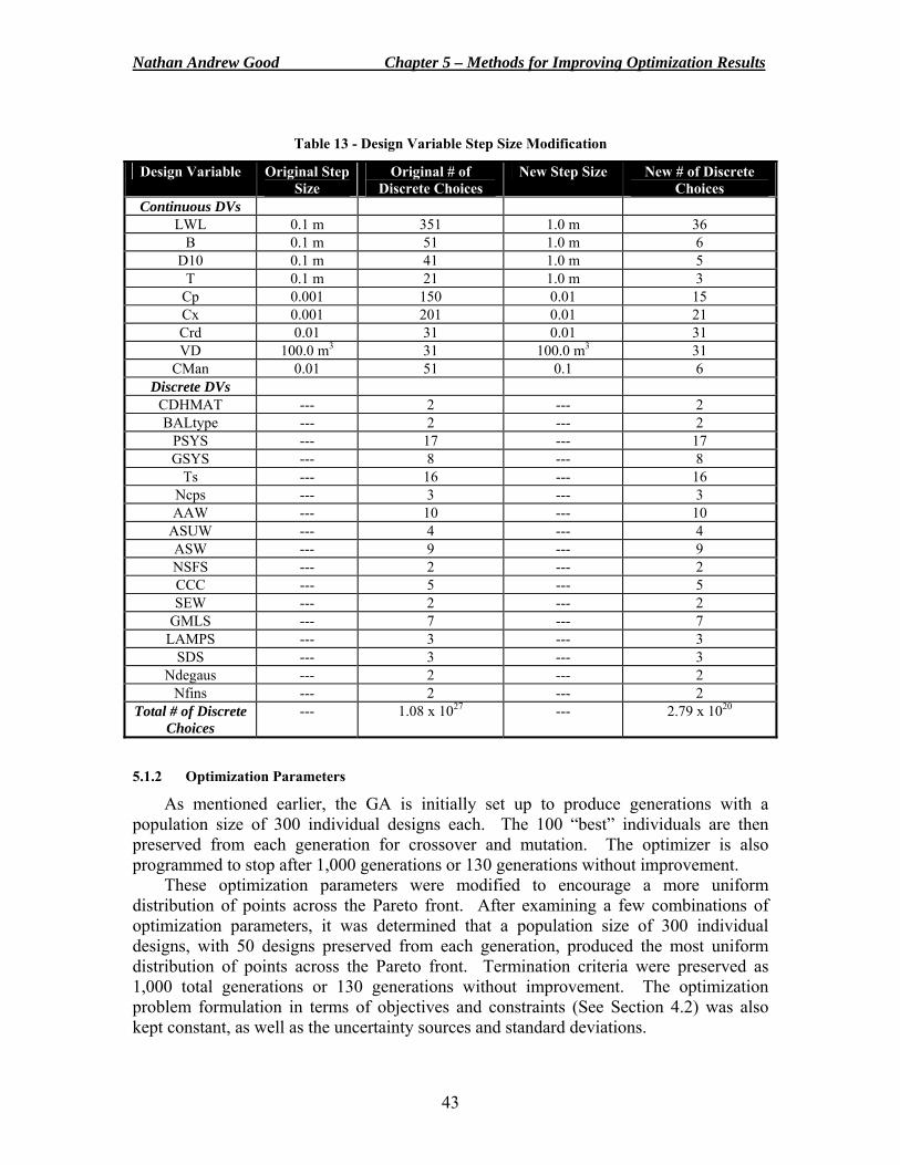
Nathan Andrew Good Chapter 5 – Methods for Improving Optimization Results
43
Table 13 - Design Variable Step Size Modification
Design Variable Original Step Size
Original # of Discrete Choices
New Step Size New # of Discrete Choices
Continuous DVs LWL 0.1 m 351 1.0 m 36
B 0.1 m 51 1.0 m 6 D10 0.1 m 41 1.0 m 5
T 0.1 m 21 1.0 m 3 Cp 0.001 150 0.01 15 Cx 0.001 201 0.01 21 Crd 0.01 31 0.01 31 VD 100.0 m3 31 100.0 m3 31
CMan 0.01 51 0.1 6 Discrete DVs
CDHMAT --- 2 --- 2 BALtype --- 2 --- 2
PSYS --- 17 --- 17 GSYS --- 8 --- 8
Ts --- 16 --- 16 Ncps --- 3 --- 3 AAW --- 10 --- 10
ASUW --- 4 --- 4 ASW --- 9 --- 9 NSFS --- 2 --- 2 CCC --- 5 --- 5 SEW --- 2 --- 2
GMLS --- 7 --- 7 LAMPS --- 3 --- 3
SDS --- 3 --- 3 Ndegaus --- 2 --- 2
Nfins --- 2 --- 2 Total # of Discrete
Choices --- 1.08 x 1027 --- 2.79 x 10²⁰
5.1.2 Optimization Parameters
As mentioned earlier, the GA is initially set up to produce generations with a population size of 300 individual designs each. The 100 “best” individuals are then preserved from each generation for crossover and mutation. The optimizer is also programmed to stop after 1,000 generations or 130 generations without improvement.
These optimization parameters were modified to encourage a more uniform distribution of points across the Pareto front. After examining a few combinations of optimization parameters, it was determined that a population size of 300 individual designs, with 50 designs preserved from each generation, produced the most uniform distribution of points across the Pareto front. Termination criteria were preserved as 1,000 total generations or 130 generations without improvement. The optimization problem formulation in terms of objectives and constraints (See Section 4.2) was also kept constant, as well as the uncertainty sources and standard deviations.
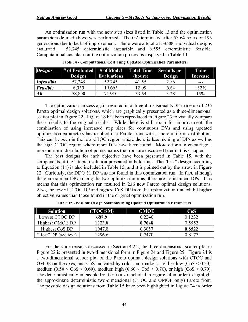
Nathan Andrew Good Chapter 5 – Methods for Improving Optimization Results
44
An optimization run with the new step sizes listed in Table 13 and the optimization parameters defined above was performed. The GA terminated after 53.64 hours or 196 generations due to lack of improvement. There were a total of 58,800 individual designs evaluated: 52,245 deterministic infeasible and 6,555 deterministic feasible. Computational cost data for the optimization process is displayed in Table 14.
Table 14 - Computational Cost using Updated Optimization Parameters
Designs # of Evaluated Designs
# of Model Evaluations
Total Time (hours)
Seconds per Design
Time Increase
Infeasible 52,245 52,245 41.55 2.86 --- Feasible 6,555 19,665 12.09 6.64 132% All 58,800 71,910 53.64 3.28 15%
The optimization process again resulted in a three-dimensional NDF made up of 236 Pareto optimal design solutions, which are graphically presented as a three-dimensional scatter plot in Figure 22. Figure 18 has been reproduced in Figure 23 to visually compare these results to the original results. While there is still room for improvement, the combination of using increased step sizes for continuous DVs and using updated optimization parameters has resulted in a Pareto front with a more uniform distribution. This can be seen in the low CTOC region where there is less niching of DPs as well as the high CTOC region where more DPs have been found. More efforts to encourage a more uniform distribution of points across the front are discussed later in this Chapter.
The best designs for each objective have been presented in Table 15, with the components of the Utopian solution presented in bold font. The “best” design according to Equation (14) is also included in Table 15, and it is pointed out by the arrow in Figure 22. Curiously, the DDG 51 DP was not found in this optimization run. In fact, although there are similar DPs among the two optimization runs, there are no identical DPs. This means that this optimization run resulted in 236 new Pareto optimal design solutions. Also, the lowest CTOC DP and highest CoS DP from this optimization run exhibit higher objective values than those found in the original optimization run.
Table 15 - Possible Design Solutions using Updated Optimization Parameters
Solution CTOC($M) OMOE CoS Lowest CTOC DP 687.9 0.2240 0.1232 Highest OMOE DP 1223.8 0.7648 0.5552
Highest CoS DP 1047.8 0.3037 0.8522 “Best” DP (see text) 1296.6 0.7470 0.8177
For the same reasons discussed in Section 4.2.2, the three-dimensional scatter plot in Figure 22 is presented in two-dimensional form in Figure 24 and Figure 25. Figure 24 is a two-dimensional scatter plot of the Pareto optimal design solutions with CTOC and OMOE on the axes, and CoS indicated by color and marker as either low (CoS < 0.50), medium (0.50 < CoS < 0.60), medium high (0.60 < CoS < 0.70), or high (CoS > 0.70). The deterministically infeasible frontier is also included in Figure 24 in order to highlight the approximate deterministic two-dimensional (CTOC and OMOE only) Pareto front. The possible design solutions from Table 15 have been highlighted in Figure 24 in order
Nathan Andrew Good Chapter 5 – Methods for Improving Optimization Results
45
to visualize their fitness relative to other possible designs. The “low” CoS level DPs and deterministically infeasible DPs are removed from the scatter plot in Figure 25 to highlight some of these other attractive designs.
Figure 22 – 3-D Scatter Plot of Pareto Optimal DPs using Updated Optimization Parameters
Figure 23 – Original 3-D NDF (Reproduction of Figure 18)
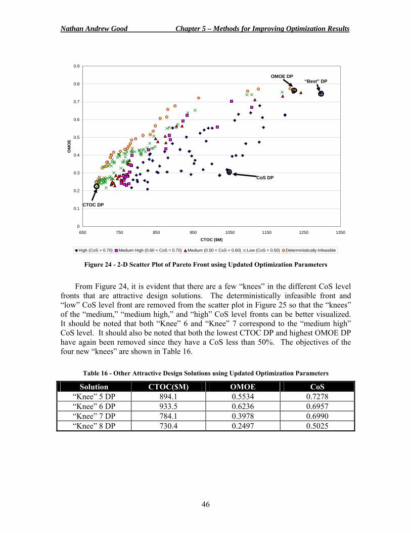
Nathan Andrew Good Chapter 5 – Methods for Improving Optimization Results
46
Figure 24 - 2-D Scatter Plot of Pareto Front using Updated Optimization Parameters
From Figure 24, it is evident that there are a few “knees” in the different CoS level
fronts that are attractive design solutions. The deterministically infeasible front and “low” CoS level front are removed from the scatter plot in Figure 25 so that the “knees” of the “medium,” “medium high,” and “high” CoS level fronts can be better visualized. It should be noted that both “Knee” 6 and “Knee” 7 correspond to the “medium high” CoS level. It should also be noted that both the lowest CTOC DP and highest OMOE DP have again been removed since they have a CoS less than 50%. The objectives of the four new “knees” are shown in Table 16.
Table 16 - Other Attractive Design Solutions using Updated Optimization Parameters
Solution CTOC($M) OMOE CoS “Knee” 5 DP 894.1 0.5534 0.7278 “Knee” 6 DP 933.5 0.6236 0.6957 “Knee” 7 DP 784.1 0.3978 0.6990 “Knee” 8 DP 730.4 0.2497 0.5025
0
0.1
0.2
0.3
0.4
0.5
0.6
0.7
0.8
0.9
650 750 850 950 1050 1150 1250 1350
CTOC ($M)
OM
OE
High (CoS > 0.70) Medium High (0.60 < CoS < 0.70) Medium (0.50 < CoS < 0.60) Low (CoS < 0.50) Deterministically Infeasible
OMOE DP “Best” DP
CoS DP
CTOC DP
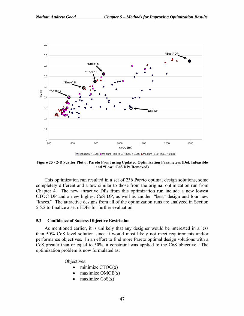
Nathan Andrew Good Chapter 5 – Methods for Improving Optimization Results
47
Figure 25 - 2-D Scatter Plot of Pareto Front using Updated Optimization Parameters (Det. Infeasible
and “Low” CoS DPs Removed)
This optimization run resulted in a set of 236 Pareto optimal design solutions, some
completely different and a few similar to those from the original optimization run from Chapter 4. The new attractive DPs from this optimization run include a new lowest CTOC DP and a new highest CoS DP, as well as another “best” design and four new “knees.” The attractive designs from all of the optimization runs are analyzed in Section 5.5.2 to finalize a set of DPs for further evaluation. 5.2 Confidence of Success Objective Restriction
As mentioned earlier, it is unlikely that any designer would be interested in a less than 50% CoS level solution since it would most likely not meet requirements and/or performance objectives. In an effort to find more Pareto optimal design solutions with a CoS greater than or equal to 50%, a constraint was applied to the CoS objective. The optimization problem is now formulated as: Objectives:
• minimize CTOC(x) • maximize OMOE(x) • maximize CoS(x)
0
0.1
0.2
0.3
0.4
0.5
0.6
0.7
0.8
0.9
700 800 900 1000 1100 1200 1300
CTOC ($M)
OM
OE
.
High (CoS > 0.70) Medium High (0.60 < CoS < 0.70) Medium (0.50 < CoS < 0.60)
“Best” DP
CoS DP
“Knee” 5
“Knee” 6
“Knee” 7
“Knee” 8
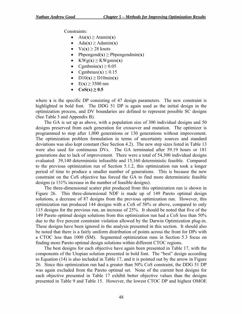
Nathan Andrew Good Chapter 5 – Methods for Improving Optimization Results
48
Constraints: • Ata(x) ≥ Atamin(x) • Ada(x) ≥ Adamin(x) • Vs(x) ≥ 28 knots • Pbpengend(x) ≥ Pbpengendmin(x) • KWg(x) ≥ KWgmin(x) • Cgmbmin(x) ≥ 0.05 • Cgmbmax(x) ≤ 0.15 • D10(x) ≥ D10min(x) • E(x) ≥ 3500 nm • CoS(x) ≥ 0.5
where x is the specific DP consisting of 47 design parameters. The new constraint is highlighted in bold font. The DDG 51 DP is again used as the initial design in the optimization process, and DV boundaries are defined to represent possible SC designs (See Table 3 and Appendix B).
The GA is set up as above, with a population size of 300 individual designs and 50 designs preserved from each generation for crossover and mutation. The optimizer is programmed to stop after 1,000 generations or 130 generations without improvement. The optimization problem formulation in terms of uncertainty sources and standard deviations was also kept constant (See Section 4.2). The new step sizes listed in Table 13 were also used for continuous DVs. The GA terminated after 59.19 hours or 181 generations due to lack of improvement. There were a total of 54,300 individual designs evaluated: 39,140 deterministic infeasible and 15,160 deterministic feasible. Compared to the previous optimization run of Section 5.1.2, this optimization run took a longer period of time to produce a smaller number of generations. This is because the new constraint on the CoS objective has forced the GA to find more deterministic feasible designs (a 131% increase in the number of feasible designs).
The three-dimensional scatter plot produced from this optimization run is shown in Figure 26. This three-dimensional NDF is made up of 149 Pareto optimal design solutions, a decrease of 87 designs from the previous optimization run. However, this optimization run produced 144 designs with a CoS of 50% or above, compared to only 115 designs for the previous run, an increase of 25%. It should be noted that five of the 149 Pareto optimal design solutions from this optimization run had a CoS less than 50% due to the five percent constraint violation allowed by the Darwin Optimization plug-in. These designs have been ignored in the analysis presented in this section. It should also be noted that there is a fairly uniform distribution of points across the front for DPs with a CTOC less than 1000 ($M). Segmented optimization runs in Section 5.3 focus on finding more Pareto optimal design solutions within different CTOC regions.
The best designs for each objective have again been presented in Table 17, with the components of the Utopian solution presented in bold font. The “best” design according to Equation (14) is also included in Table 17, and it is pointed out by the arrow in Figure 26. Since this optimization run had a greater than 50% CoS constraint, the DDG 51 DP was again excluded from the Pareto optimal set. None of the current best designs for each objective presented in Table 17 exhibit better objective values than the designs presented in Table 9 and Table 15. However, the lowest CTOC DP and highest OMOE
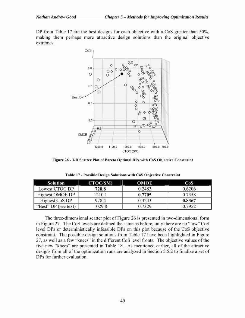
Nathan Andrew Good Chapter 5 – Methods for Improving Optimization Results
49
DP from Table 17 are the best designs for each objective with a CoS greater than 50%, making them perhaps more attractive design solutions than the original objective extremes.
Figure 26 - 3-D Scatter Plot of Pareto Optimal DPs with CoS Objective Constraint
Table 17 - Possible Design Solutions with CoS Objective Constraint
Solution CTOC($M) OMOE CoS Lowest CTOC DP 728.8 0.2483 0.6206 Highest OMOE DP 1210.1 0.7705 0.7358
Highest CoS DP 978.4 0.3243 0.8367 “Best” DP (see text) 1029.8 0.7329 0.7952
The three-dimensional scatter plot of Figure 26 is presented in two-dimensional form in Figure 27. The CoS levels are defined the same as before, only there are no “low” CoS level DPs or deterministically infeasible DPs on this plot because of the CoS objective constraint. The possible design solutions from Table 17 have been highlighted in Figure 27, as well as a few “knees” in the different CoS level fronts. The objective values of the five new “knees” are presented in Table 18. As mentioned earlier, all of the attractive designs from all of the optimization runs are analyzed in Section 5.5.2 to finalize a set of DPs for further evaluation.
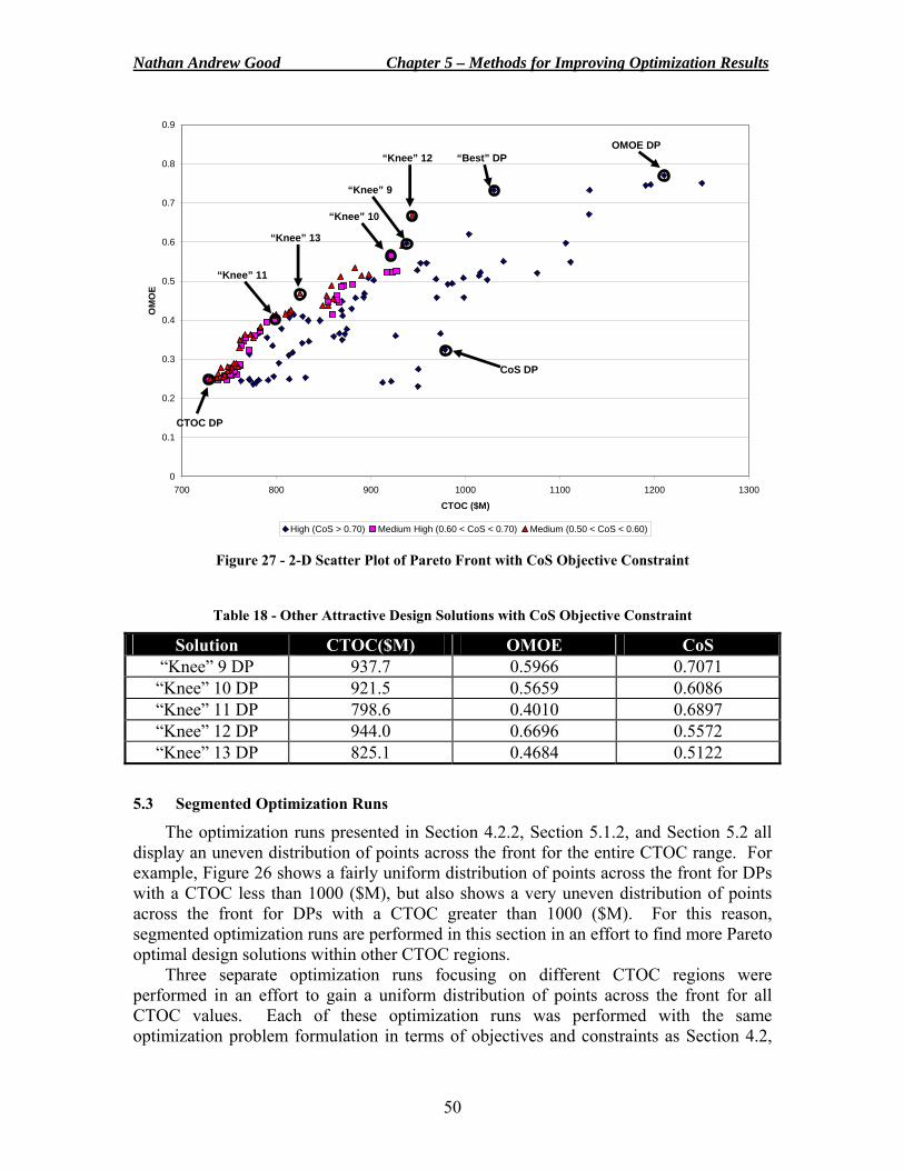
Nathan Andrew Good Chapter 5 – Methods for Improving Optimization Results
50
Figure 27 - 2-D Scatter Plot of Pareto Front with CoS Objective Constraint
Table 18 - Other Attractive Design Solutions with CoS Objective Constraint
Solution CTOC($M) OMOE CoS “Knee” 9 DP 937.7 0.5966 0.7071 “Knee” 10 DP 921.5 0.5659 0.6086 “Knee” 11 DP 798.6 0.4010 0.6897 “Knee” 12 DP 944.0 0.6696 0.5572 “Knee” 13 DP 825.1 0.4684 0.5122
5.3 Segmented Optimization Runs
The optimization runs presented in Section 4.2.2, Section 5.1.2, and Section 5.2 all display an uneven distribution of points across the front for the entire CTOC range. For example, Figure 26 shows a fairly uniform distribution of points across the front for DPs with a CTOC less than 1000 ($M), but also shows a very uneven distribution of points across the front for DPs with a CTOC greater than 1000 ($M). For this reason, segmented optimization runs are performed in this section in an effort to find more Pareto optimal design solutions within other CTOC regions.
Three separate optimization runs focusing on different CTOC regions were performed in an effort to gain a uniform distribution of points across the front for all CTOC values. Each of these optimization runs was performed with the same optimization problem formulation in terms of objectives and constraints as Section 4.2,
0
0.1
0.2
0.3
0.4
0.5
0.6
0.7
0.8
0.9
700 800 900 1000 1100 1200 1300
CTOC ($M)
OM
OE
High (CoS > 0.70) Medium High (0.60 < CoS < 0.70) Medium (0.50 < CoS < 0.60)
OMOE DP “Best” DP
CoS DP
CTOC DP
“Knee” 9
“Knee” 10
“Knee” 11
“Knee” 12
“Knee” 13
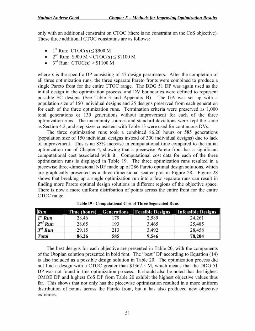
Nathan Andrew Good Chapter 5 – Methods for Improving Optimization Results
51
only with an additional constraint on CTOC (there is no constraint on the CoS objective). These three additional CTOC constraints are as follows:
• 1st Run: CTOC(x) ≤ $900 M • 2nd Run: $900 M < CTOC(x) ≤ $1100 M • 3rd Run: CTOC(x) > $1100 M
where x is the specific DP consisting of 47 design parameters. After the completion of all three optimization runs, the three separate Pareto fronts were combined to produce a single Pareto front for the entire CTOC range. The DDG 51 DP was again used as the initial design in the optimization process, and DV boundaries were defined to represent possible SC designs (See Table 3 and Appendix B). The GA was set up with a population size of 150 individual designs and 25 designs preserved from each generation for each of the three optimization runs. Termination criteria were preserved as 1,000 total generations or 130 generations without improvement for each of the three optimization runs. The uncertainty sources and standard deviations were kept the same as Section 4.2, and step sizes consistent with Table 13 were used for continuous DVs.
The three optimization runs took a combined 86.26 hours or 585 generations (population size of 150 individual designs instead of 300 individual designs) due to lack of improvement. This is an 85% increase in computational time compared to the initial optimization run of Chapter 4, showing that a piecewise Pareto front has a significant computational cost associated with it. Computational cost data for each of the three optimization runs is displayed in Table 19. The three optimization runs resulted in a piecewise three-dimensional NDF made up of 286 Pareto optimal design solutions, which are graphically presented as a three-dimensional scatter plot in Figure 28. Figure 28 shows that breaking up a single optimization run into a few separate runs can result in finding more Pareto optimal design solutions in different regions of the objective space. There is now a more uniform distribution of points across the entire front for the entire CTOC range.
Table 19 - Computational Cost of Three Segmented Runs
Run Time (hours) Generations Feasible Designs Infeasible Designs 1st Run 28.46 179 2,589 24,261 2nd Run 28.65 193 3,465 25,485 3rd Run 29.15 213 3,492 28,458 Total 86.26 585 9,546 78,204
The best designs for each objective are presented in Table 20, with the components of the Utopian solution presented in bold font. The “best” DP according to Equation (14) is also included as a possible design solution in Table 20. The optimization process did not find a design with a CTOC greater than $1367.5 M, which means that the DDG 51 DP was not found in this optimization process. It should also be noted that the highest OMOE DP and highest CoS DP from Table 20 exhibit the highest objective values thus far. This shows that not only has the piecewise optimization resulted in a more uniform distribution of points across the Pareto front, but it has also produced new objective extremes.
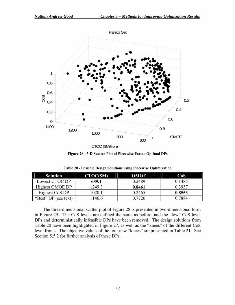
Nathan Andrew Good Chapter 5 – Methods for Improving Optimization Results
52
600800
10001200
1400
0.2
0.4
0.6
0.8
1
0
0.2
0.4
0.6
0.8
1
CTOC ($Million)
OMOE
CoS
Pareto Set
Figure 28 - 3-D Scatter Plot of Piecewise Pareto Optimal DPs
Table 20 - Possible Design Solutions using Piecewise Optimization
Solution CTOC($M) OMOE CoS Lowest CTOC DP 689.1 0.2489 0.1485 Highest OMOE DP 1249.3 0.8461 0.3937
Highest CoS DP 1020.1 0.2465 0.8553 “Best” DP (see text) 1146.6 0.7726 0.7884
The three-dimensional scatter plot of Figure 28 is presented in two-dimensional form in Figure 29. The CoS levels are defined the same as before, and the “low” CoS level DPs and deterministically infeasible DPs have been removed. The design solutions from Table 20 have been highlighted in Figure 27, as well as the “knees” of the different CoS level fronts. The objective values of the four new “knees” are presented in Table 21. See Section 5.5.2 for further analysis of these DPs.
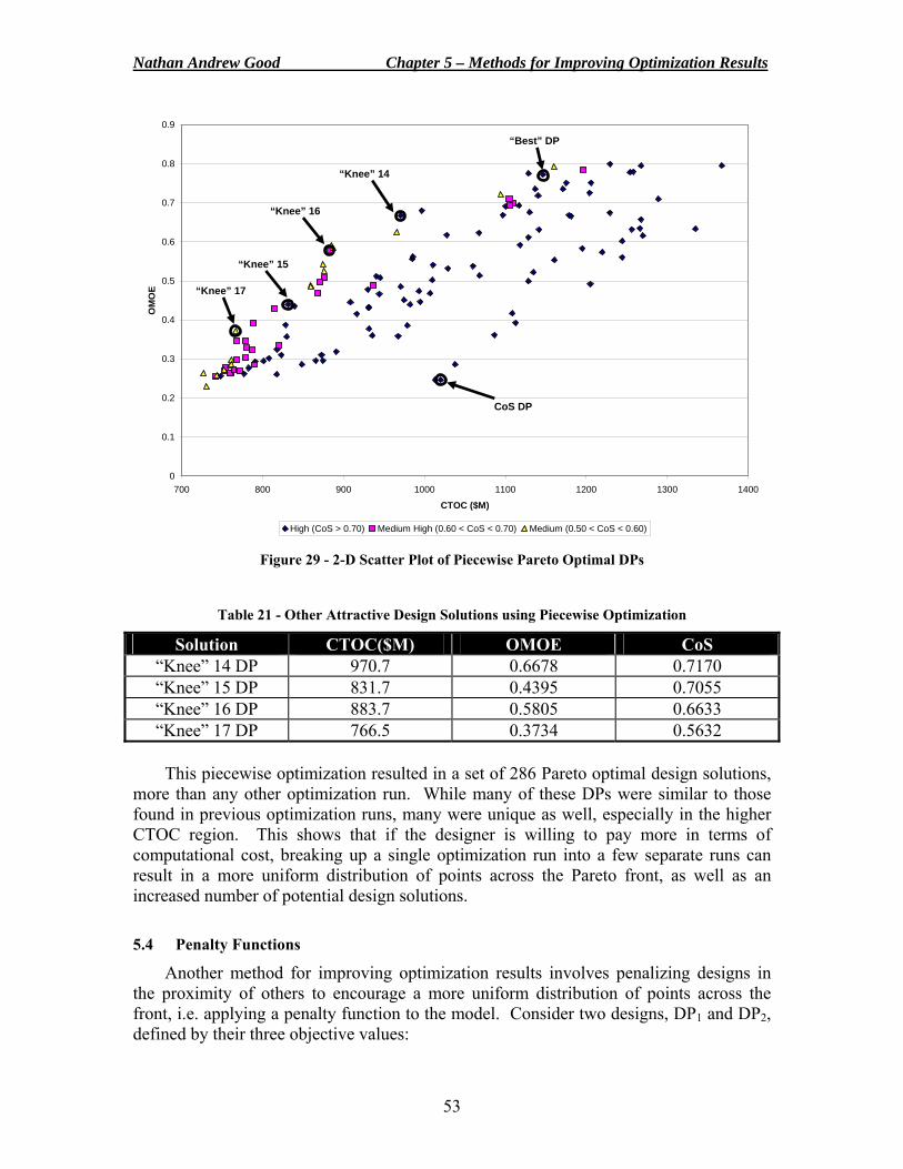
Nathan Andrew Good Chapter 5 – Methods for Improving Optimization Results
53
Figure 29 - 2-D Scatter Plot of Piecewise Pareto Optimal DPs
Table 21 - Other Attractive Design Solutions using Piecewise Optimization
Solution CTOC($M) OMOE CoS “Knee” 14 DP 970.7 0.6678 0.7170 “Knee” 15 DP 831.7 0.4395 0.7055 “Knee” 16 DP 883.7 0.5805 0.6633 “Knee” 17 DP 766.5 0.3734 0.5632
This piecewise optimization resulted in a set of 286 Pareto optimal design solutions,
more than any other optimization run. While many of these DPs were similar to those found in previous optimization runs, many were unique as well, especially in the higher CTOC region. This shows that if the designer is willing to pay more in terms of computational cost, breaking up a single optimization run into a few separate runs can result in a more uniform distribution of points across the Pareto front, as well as an increased number of potential design solutions. 5.4 Penalty Functions
Another method for improving optimization results involves penalizing designs in the proximity of others to encourage a more uniform distribution of points across the front, i.e. applying a penalty function to the model. Consider two designs, DP1 and DP2, defined by their three objective values:
0
0.1
0.2
0.3
0.4
0.5
0.6
0.7
0.8
0.9
700 800 900 1000 1100 1200 1300 1400
CTOC ($M)
OM
OE
High (CoS > 0.70) Medium High (0.60 < CoS < 0.70) Medium (0.50 < CoS < 0.60)
“Best” DP
CoS DP
“Knee” 14
“Knee” 15
“Knee” 16
“Knee” 17
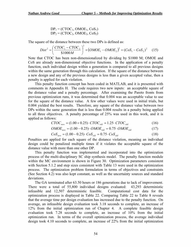
Nathan Andrew Good Chapter 5 – Methods for Improving Optimization Results
54
DP1 = (CTOC1, OMOE1, CoS1) DP2 = (CTOC2, OMOE2, CoS2) The square of the distance between these two DPs is defined as:
( ) 221
221
2212 )(
1000$CoSCoSOMOEOMOE
MCTOCCTOC
Dist −+−+⎟⎠⎞
⎜⎝⎛ −
= (15)
Note that CTOC has been non-dimensionalized by dividing by $1000 M; OMOE and CoS are already non-dimensional objective functions. In the application of a penalty function, each individual design within a generation is compared to all previous designs within the same generation through this calculation. If the square of the distance between a new design and any of the previous designs is less than a given accepted value, then a penalty is applied for each violation.
This penalty function concept has been coded in MATLAB, and it is presented with comments in Appendix H. The code requires two new inputs: an acceptable square of the distance value and a penalty percentage. After examining the Pareto fronts from previous optimization runs, it was determined that 0.004 was an acceptable value to use for the square of the distance value. A few other values were used in initial trials, but 0.004 yielded the best results. Therefore, any square of the distance value between two DPs within the same generation that is less than 0.004 results in a penalty being applied to all three objectives. A penalty percentage of 25% was used in this work, and it is applied as follows:
oldoldnew CTOCCTOCCTOC ⋅=⋅+= 25.1)25.000.1( (16) oldoldnew OMOEOMOEOMOE ⋅=⋅−= 75.0)25.000.1( (17) oldoldnew CoSCoSCoS ⋅=⋅−= 75.0)25.000.1( (18)
Penalties are applied for each square of the distance violation, meaning an individual design could be penalized multiple times if it violates the acceptable square of the distance value with more than one other DP.
This penalty function was implemented and incorporated into the optimization process of the multi-disciplinary SC ship synthesis model. The penalty function module within the MC environment is shown in Figure 30. Optimization parameters consistent with Section 5.1.2 and step sizes consistent with Table 13 were used in the optimization process. The optimization problem formulation in terms of objectives and constraints (See Section 4.2) was also kept constant, as well as the uncertainty sources and standard deviations.
The GA terminated after 63.50 hours or 186 generations due to lack of improvement. There were a total of 55,800 individual designs evaluated: 43,293 deterministic infeasible and 12,507 deterministic feasible. Computational cost data for the optimization process is displayed in Table 22. Comparing Table 22 to Table 8 reveals that the average time per design evaluation has increased due to the penalty function. On average, an infeasible design evaluation took 3.18 seconds to complete, an increase of 12% from the initial optimization run of Chapter 4. A complete feasible design evaluation took 7.28 seconds to complete, an increase of 10% from the initial optimization run. In terms of the overall optimization process, the average individual design took 4.10 seconds to complete, an increase of 22% from the initial optimization
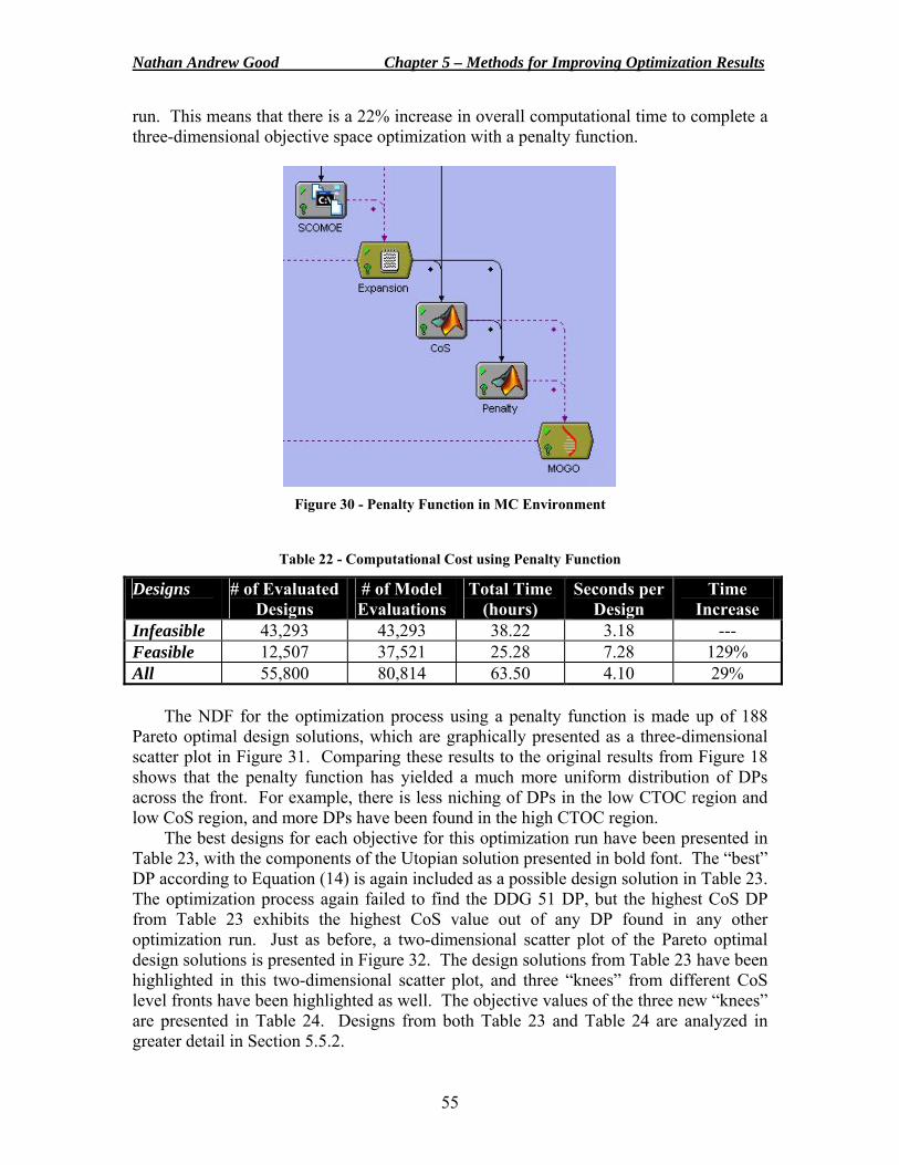
Nathan Andrew Good Chapter 5 – Methods for Improving Optimization Results
55
run. This means that there is a 22% increase in overall computational time to complete a three-dimensional objective space optimization with a penalty function.
Figure 30 - Penalty Function in MC Environment
Table 22 - Computational Cost using Penalty Function
Designs # of Evaluated Designs
# of Model Evaluations
Total Time (hours)
Seconds per Design
Time Increase
Infeasible 43,293 43,293 38.22 3.18 --- Feasible 12,507 37,521 25.28 7.28 129% All 55,800 80,814 63.50 4.10 29%
The NDF for the optimization process using a penalty function is made up of 188 Pareto optimal design solutions, which are graphically presented as a three-dimensional scatter plot in Figure 31. Comparing these results to the original results from Figure 18 shows that the penalty function has yielded a much more uniform distribution of DPs across the front. For example, there is less niching of DPs in the low CTOC region and low CoS region, and more DPs have been found in the high CTOC region.
The best designs for each objective for this optimization run have been presented in Table 23, with the components of the Utopian solution presented in bold font. The “best” DP according to Equation (14) is again included as a possible design solution in Table 23. The optimization process again failed to find the DDG 51 DP, but the highest CoS DP from Table 23 exhibits the highest CoS value out of any DP found in any other optimization run. Just as before, a two-dimensional scatter plot of the Pareto optimal design solutions is presented in Figure 32. The design solutions from Table 23 have been highlighted in this two-dimensional scatter plot, and three “knees” from different CoS level fronts have been highlighted as well. The objective values of the three new “knees” are presented in Table 24. Designs from both Table 23 and Table 24 are analyzed in greater detail in Section 5.5.2.
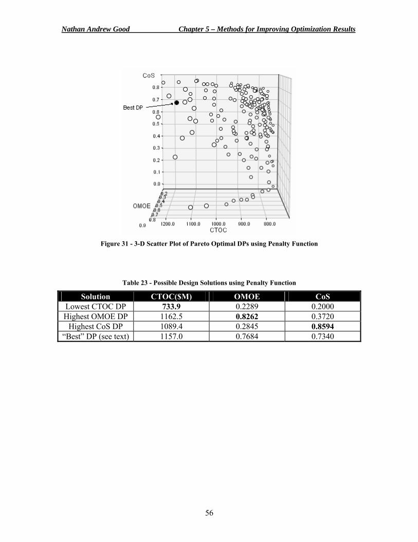
Nathan Andrew Good Chapter 5 – Methods for Improving Optimization Results
56
Figure 31 - 3-D Scatter Plot of Pareto Optimal DPs using Penalty Function
Table 23 - Possible Design Solutions using Penalty Function
Solution CTOC($M) OMOE CoS Lowest CTOC DP 733.9 0.2289 0.2000 Highest OMOE DP 1162.5 0.8262 0.3720
Highest CoS DP 1089.4 0.2845 0.8594 “Best” DP (see text) 1157.0 0.7684 0.7340
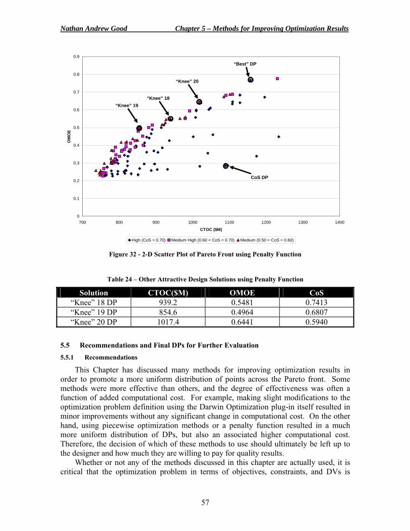
Nathan Andrew Good Chapter 5 – Methods for Improving Optimization Results
57
Figure 32 - 2-D Scatter Plot of Pareto Front using Penalty Function
Table 24 – Other Attractive Design Solutions using Penalty Function
Solution CTOC($M) OMOE CoS “Knee” 18 DP 939.2 0.5481 0.7413 “Knee” 19 DP 854.6 0.4964 0.6807 “Knee” 20 DP 1017.4 0.6441 0.5940
5.5 Recommendations and Final DPs for Further Evaluation 5.5.1 Recommendations
This Chapter has discussed many methods for improving optimization results in order to promote a more uniform distribution of points across the Pareto front. Some methods were more effective than others, and the degree of effectiveness was often a function of added computational cost. For example, making slight modifications to the optimization problem definition using the Darwin Optimization plug-in itself resulted in minor improvements without any significant change in computational cost. On the other hand, using piecewise optimization methods or a penalty function resulted in a much more uniform distribution of DPs, but also an associated higher computational cost. Therefore, the decision of which of these methods to use should ultimately be left up to the designer and how much they are willing to pay for quality results.
Whether or not any of the methods discussed in this chapter are actually used, it is critical that the optimization problem in terms of objectives, constraints, and DVs is
0
0.1
0.2
0.3
0.4
0.5
0.6
0.7
0.8
0.9
700 800 900 1000 1100 1200 1300 1400
CTOC ($M)
OM
OE
High (CoS > 0.70) Medium High (0.60 < CoS < 0.70) Medium (0.50 < CoS < 0.60)
“Best” DP
CoS DP
“Knee” 18“Knee” 19
“Knee” 20
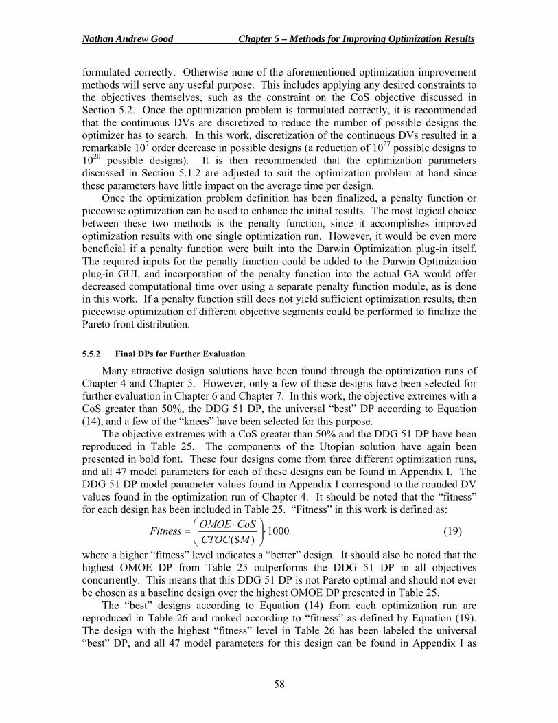
Nathan Andrew Good Chapter 5 – Methods for Improving Optimization Results
58
formulated correctly. Otherwise none of the aforementioned optimization improvement methods will serve any useful purpose. This includes applying any desired constraints to the objectives themselves, such as the constraint on the CoS objective discussed in Section 5.2. Once the optimization problem is formulated correctly, it is recommended that the continuous DVs are discretized to reduce the number of possible designs the optimizer has to search. In this work, discretization of the continuous DVs resulted in a remarkable 107 order decrease in possible designs (a reduction of 1027 possible designs to 1020 possible designs). It is then recommended that the optimization parameters discussed in Section 5.1.2 are adjusted to suit the optimization problem at hand since these parameters have little impact on the average time per design.
Once the optimization problem definition has been finalized, a penalty function or piecewise optimization can be used to enhance the initial results. The most logical choice between these two methods is the penalty function, since it accomplishes improved optimization results with one single optimization run. However, it would be even more beneficial if a penalty function were built into the Darwin Optimization plug-in itself. The required inputs for the penalty function could be added to the Darwin Optimization plug-in GUI, and incorporation of the penalty function into the actual GA would offer decreased computational time over using a separate penalty function module, as is done in this work. If a penalty function still does not yield sufficient optimization results, then piecewise optimization of different objective segments could be performed to finalize the Pareto front distribution. 5.5.2 Final DPs for Further Evaluation
Many attractive design solutions have been found through the optimization runs of Chapter 4 and Chapter 5. However, only a few of these designs have been selected for further evaluation in Chapter 6 and Chapter 7. In this work, the objective extremes with a CoS greater than 50%, the DDG 51 DP, the universal “best” DP according to Equation (14), and a few of the “knees” have been selected for this purpose.
The objective extremes with a CoS greater than 50% and the DDG 51 DP have been reproduced in Table 25. The components of the Utopian solution have again been presented in bold font. These four designs come from three different optimization runs, and all 47 model parameters for each of these designs can be found in Appendix I. The DDG 51 DP model parameter values found in Appendix I correspond to the rounded DV values found in the optimization run of Chapter 4. It should be noted that the “fitness” for each design has been included in Table 25. “Fitness” in this work is defined as:
1000)($
⋅⎟⎟⎠
⎞⎜⎜⎝
⎛ ⋅=
MCTOCCoSOMOEFitness (19)
where a higher “fitness” level indicates a “better” design. It should also be noted that the highest OMOE DP from Table 25 outperforms the DDG 51 DP in all objectives concurrently. This means that this DDG 51 DP is not Pareto optimal and should not ever be chosen as a baseline design over the highest OMOE DP presented in Table 25.
The “best” designs according to Equation (14) from each optimization run are reproduced in Table 26 and ranked according to “fitness” as defined by Equation (19). The design with the highest “fitness” level in Table 26 has been labeled the universal “best” DP, and all 47 model parameters for this design can be found in Appendix I as
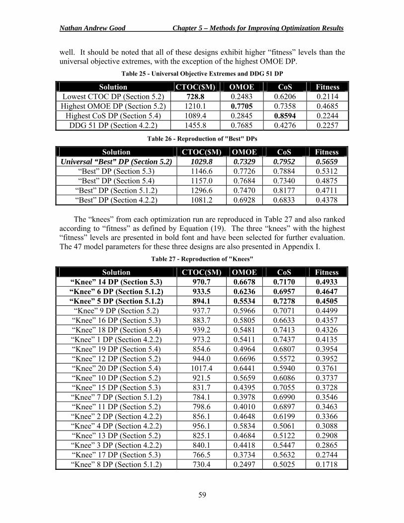
Nathan Andrew Good Chapter 5 – Methods for Improving Optimization Results
59
well. It should be noted that all of these designs exhibit higher “fitness” levels than the universal objective extremes, with the exception of the highest OMOE DP.
Table 25 - Universal Objective Extremes and DDG 51 DP
Solution CTOC($M) OMOE CoS Fitness Lowest CTOC DP (Section 5.2) 728.8 0.2483 0.6206 0.2114 Highest OMOE DP (Section 5.2) 1210.1 0.7705 0.7358 0.4685
Highest CoS DP (Section 5.4) 1089.4 0.2845 0.8594 0.2244 DDG 51 DP (Section 4.2.2) 1455.8 0.7685 0.4276 0.2257
Table 26 - Reproduction of "Best" DPs
Solution CTOC($M) OMOE CoS Fitness Universal “Best” DP (Section 5.2) 1029.8 0.7329 0.7952 0.5659
“Best” DP (Section 5.3) 1146.6 0.7726 0.7884 0.5312 “Best” DP (Section 5.4) 1157.0 0.7684 0.7340 0.4875
“Best” DP (Section 5.1.2) 1296.6 0.7470 0.8177 0.4711 “Best” DP (Section 4.2.2) 1081.2 0.6928 0.6833 0.4378
The “knees” from each optimization run are reproduced in Table 27 and also ranked
according to “fitness” as defined by Equation (19). The three “knees” with the highest “fitness” levels are presented in bold font and have been selected for further evaluation. The 47 model parameters for these three designs are also presented in Appendix I.
Table 27 - Reproduction of "Knees"
Solution CTOC($M) OMOE CoS Fitness “Knee” 14 DP (Section 5.3) 970.7 0.6678 0.7170 0.4933 “Knee” 6 DP (Section 5.1.2) 933.5 0.6236 0.6957 0.4647 “Knee” 5 DP (Section 5.1.2) 894.1 0.5534 0.7278 0.4505
“Knee” 9 DP (Section 5.2) 937.7 0.5966 0.7071 0.4499 “Knee” 16 DP (Section 5.3) 883.7 0.5805 0.6633 0.4357 “Knee” 18 DP (Section 5.4) 939.2 0.5481 0.7413 0.4326 “Knee” 1 DP (Section 4.2.2) 973.2 0.5411 0.7437 0.4135 “Knee” 19 DP (Section 5.4) 854.6 0.4964 0.6807 0.3954 “Knee” 12 DP (Section 5.2) 944.0 0.6696 0.5572 0.3952 “Knee” 20 DP (Section 5.4) 1017.4 0.6441 0.5940 0.3761 “Knee” 10 DP (Section 5.2) 921.5 0.5659 0.6086 0.3737 “Knee” 15 DP (Section 5.3) 831.7 0.4395 0.7055 0.3728 “Knee” 7 DP (Section 5.1.2) 784.1 0.3978 0.6990 0.3546 “Knee” 11 DP (Section 5.2) 798.6 0.4010 0.6897 0.3463 “Knee” 2 DP (Section 4.2.2) 856.1 0.4648 0.6199 0.3366 “Knee” 4 DP (Section 4.2.2) 956.1 0.5834 0.5061 0.3088 “Knee” 13 DP (Section 5.2) 825.1 0.4684 0.5122 0.2908 “Knee” 3 DP (Section 4.2.2) 840.1 0.4418 0.5447 0.2865 “Knee” 17 DP (Section 5.3) 766.5 0.3734 0.5632 0.2744 “Knee” 8 DP (Section 5.1.2) 730.4 0.2497 0.5025 0.1718
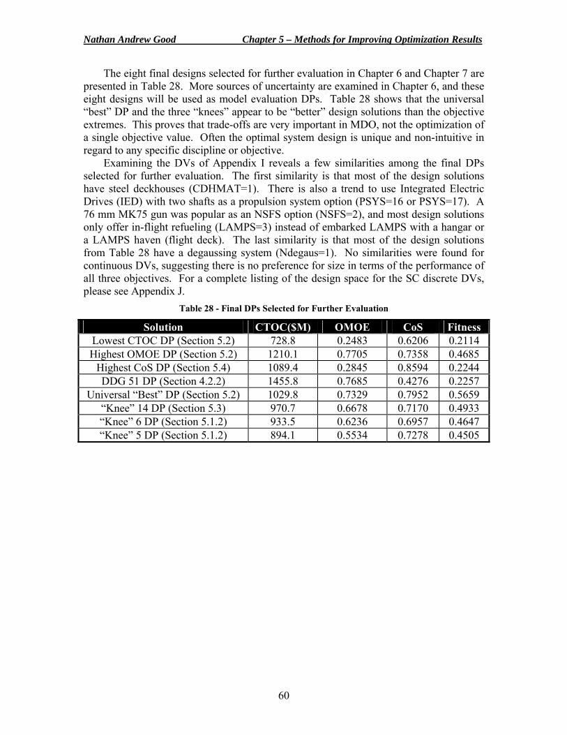
Nathan Andrew Good Chapter 5 – Methods for Improving Optimization Results
60
The eight final designs selected for further evaluation in Chapter 6 and Chapter 7 are presented in Table 28. More sources of uncertainty are examined in Chapter 6, and these eight designs will be used as model evaluation DPs. Table 28 shows that the universal “best” DP and the three “knees” appear to be “better” design solutions than the objective extremes. This proves that trade-offs are very important in MDO, not the optimization of a single objective value. Often the optimal system design is unique and non-intuitive in regard to any specific discipline or objective.
Examining the DVs of Appendix I reveals a few similarities among the final DPs selected for further evaluation. The first similarity is that most of the design solutions have steel deckhouses (CDHMAT=1). There is also a trend to use Integrated Electric Drives (IED) with two shafts as a propulsion system option (PSYS=16 or PSYS=17). A 76 mm MK75 gun was popular as an NSFS option (NSFS=2), and most design solutions only offer in-flight refueling (LAMPS=3) instead of embarked LAMPS with a hangar or a LAMPS haven (flight deck). The last similarity is that most of the design solutions from Table 28 have a degaussing system (Ndegaus=1). No similarities were found for continuous DVs, suggesting there is no preference for size in terms of the performance of all three objectives. For a complete listing of the design space for the SC discrete DVs, please see Appendix J.
Table 28 - Final DPs Selected for Further Evaluation
Solution CTOC($M) OMOE CoS Fitness Lowest CTOC DP (Section 5.2) 728.8 0.2483 0.6206 0.2114 Highest OMOE DP (Section 5.2) 1210.1 0.7705 0.7358 0.4685
Highest CoS DP (Section 5.4) 1089.4 0.2845 0.8594 0.2244 DDG 51 DP (Section 4.2.2) 1455.8 0.7685 0.4276 0.2257
Universal “Best” DP (Section 5.2) 1029.8 0.7329 0.7952 0.5659 “Knee” 14 DP (Section 5.3) 970.7 0.6678 0.7170 0.4933 “Knee” 6 DP (Section 5.1.2) 933.5 0.6236 0.6957 0.4647 “Knee” 5 DP (Section 5.1.2) 894.1 0.5534 0.7278 0.4505
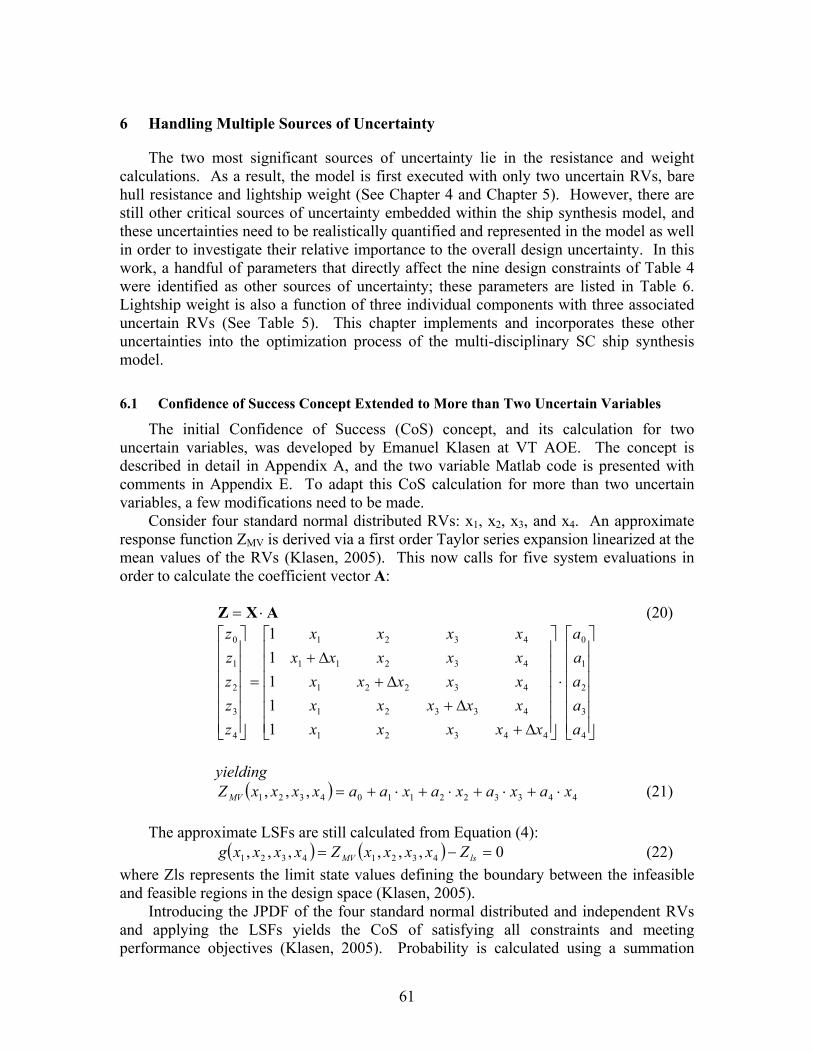
61
6 Handling Multiple Sources of Uncertainty
The two most significant sources of uncertainty lie in the resistance and weight calculations. As a result, the model is first executed with only two uncertain RVs, bare hull resistance and lightship weight (See Chapter 4 and Chapter 5). However, there are still other critical sources of uncertainty embedded within the ship synthesis model, and these uncertainties need to be realistically quantified and represented in the model as well in order to investigate their relative importance to the overall design uncertainty. In this work, a handful of parameters that directly affect the nine design constraints of Table 4 were identified as other sources of uncertainty; these parameters are listed in Table 6. Lightship weight is also a function of three individual components with three associated uncertain RVs (See Table 5). This chapter implements and incorporates these other uncertainties into the optimization process of the multi-disciplinary SC ship synthesis model. 6.1 Confidence of Success Concept Extended to More than Two Uncertain Variables
The initial Confidence of Success (CoS) concept, and its calculation for two uncertain variables, was developed by Emanuel Klasen at VT AOE. The concept is described in detail in Appendix A, and the two variable Matlab code is presented with comments in Appendix E. To adapt this CoS calculation for more than two uncertain variables, a few modifications need to be made.
Consider four standard normal distributed RVs: x1, x2, x3, and x4. An approximate response function ZMV is derived via a first order Taylor series expansion linearized at the mean values of the RVs (Klasen, 2005). This now calls for five system evaluations in order to calculate the coefficient vector A:
AXZ ⋅= (20)
⎥⎥⎥⎥⎥⎥
⎦
⎤
⎢⎢⎢⎢⎢⎢
⎣
⎡
⋅
⎥⎥⎥⎥⎥⎥
⎦
⎤
⎢⎢⎢⎢⎢⎢
⎣
⎡
Δ+Δ+
Δ+Δ+
=
⎥⎥⎥⎥⎥⎥
⎦
⎤
⎢⎢⎢⎢⎢⎢
⎣
⎡
4
3
2
1
0
44321
43321
43221
43211
4321
4
3
2
1
0
11111
aaaaa
xxxxxxxxxxxxxxxxxxxxxxxx
zzzzz
yielding
( ) 4433221104321 ,,, xaxaxaxaaxxxxZ MV ⋅+⋅+⋅+⋅+= (21)
The approximate LSFs are still calculated from Equation (4): ( ) ( ) 0,,,,,, 43214321 =−= lsMV ZxxxxZxxxxg (22) where Zls represents the limit state values defining the boundary between the infeasible and feasible regions in the design space (Klasen, 2005).
Introducing the JPDF of the four standard normal distributed and independent RVs and applying the LSFs yields the CoS of satisfying all constraints and meeting performance objectives (Klasen, 2005). Probability is calculated using a summation
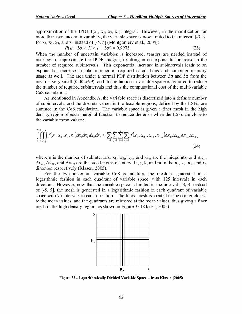
Nathan Andrew Good Chapter 6 – Handling Multiple Sources of Uncertainty
62
approximation of the JPDF f(x1, x2, x3, x4) integral. However, in the modification for more than two uncertain variables, the variable space is now limited to the interval [-3, 3] for x1, x2, x3, and x4 instead of [-5, 5] (Montgomery et al., 2004):
9973.0)33( =+<<− σμσμ XP (23) When the number of uncertain variables is increased, tensors are needed instead of matrices to approximate the JPDF integral, resulting in an exponential increase in the number of required subintervals. This exponential increase in subintervals leads to an exponential increase in total number of required calculations and computer memory usage as well. The area under a normal PDF distribution between 3σ and 5σ from the mean is very small (0.002699), and this reduction in variable space is required to reduce the number of required subintervals and thus the computational cost of the multi-variable CoS calculation.
As mentioned in Appendix A, the variable space is discretized into a definite number of subintervals, and the discrete values in the feasible regions, defined by the LSFs, are summed in the CoS calculation. The variable space is given a finer mesh in the high density region of each marginal function to reduce the error when the LSFs are close to the variable mean values:
( ) ( )∫ ∫ ∫ ∫ ∑∑∑∑= = = =
ΔΔΔΔ≈b
a
d
c
f
e
h
g
n
i
n
j
n
k
n
mmkjimkji xxxxxxxxfdxdxdxdxxxxxf
1 1 1 14321432143214321 ,,,,,,
(24)
where n is the number of subintervals, x1i, x2j, x3k, and x4m are the midpoints, and Δx1i, Δx2j, Δx3k, and Δx4m are the side lengths of interval i, j, k, and m in the x1, x2, x3, and x4 direction respectively (Klasen, 2005).
For the two uncertain variable CoS calculation, the mesh is generated in a logarithmic fashion in each quadrant of variable space, with 125 intervals in each direction. However, now that the variable space is limited to the interval [-3, 3] instead of [-5, 5], the mesh is generated in a logarithmic fashion in each quadrant of variable space with 75 intervals in each direction. The finest mesh is located in the corner closest to the mean values, and the quadrants are mirrored at the mean values, thus giving a finer mesh in the high density region, as shown in Figure 33 (Klasen, 2005).
x
y
μx
μy
Figure 33 - Logarithmically Divided Variable Space – from Klasen (2005)
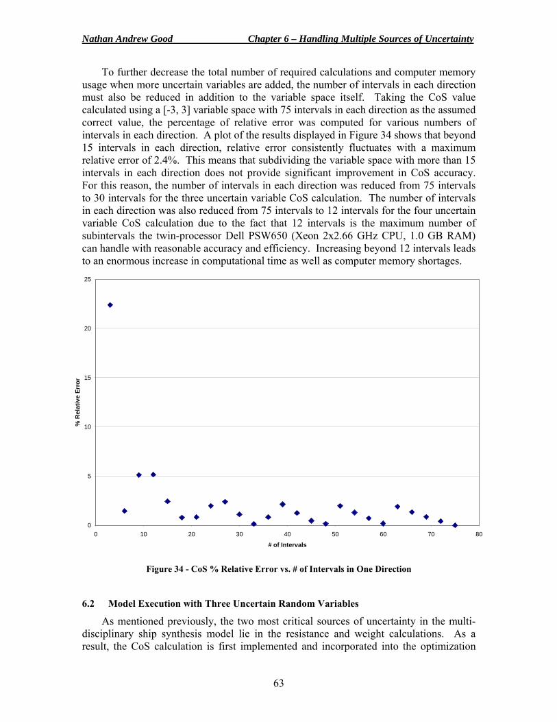
Nathan Andrew Good Chapter 6 – Handling Multiple Sources of Uncertainty
63
To further decrease the total number of required calculations and computer memory usage when more uncertain variables are added, the number of intervals in each direction must also be reduced in addition to the variable space itself. Taking the CoS value calculated using a [-3, 3] variable space with 75 intervals in each direction as the assumed correct value, the percentage of relative error was computed for various numbers of intervals in each direction. A plot of the results displayed in Figure 34 shows that beyond 15 intervals in each direction, relative error consistently fluctuates with a maximum relative error of 2.4%. This means that subdividing the variable space with more than 15 intervals in each direction does not provide significant improvement in CoS accuracy. For this reason, the number of intervals in each direction was reduced from 75 intervals to 30 intervals for the three uncertain variable CoS calculation. The number of intervals in each direction was also reduced from 75 intervals to 12 intervals for the four uncertain variable CoS calculation due to the fact that 12 intervals is the maximum number of subintervals the twin-processor Dell PSW650 (Xeon 2x2.66 GHz CPU, 1.0 GB RAM) can handle with reasonable accuracy and efficiency. Increasing beyond 12 intervals leads to an enormous increase in computational time as well as computer memory shortages.
0
5
10
15
20
25
0 10 20 30 40 50 60 70 80
# of Intervals
% R
elat
ive
Erro
r
Figure 34 - CoS % Relative Error vs. # of Intervals in One Direction
6.2 Model Execution with Three Uncertain Random Variables
As mentioned previously, the two most critical sources of uncertainty in the multi-disciplinary ship synthesis model lie in the resistance and weight calculations. As a result, the CoS calculation is first implemented and incorporated into the optimization
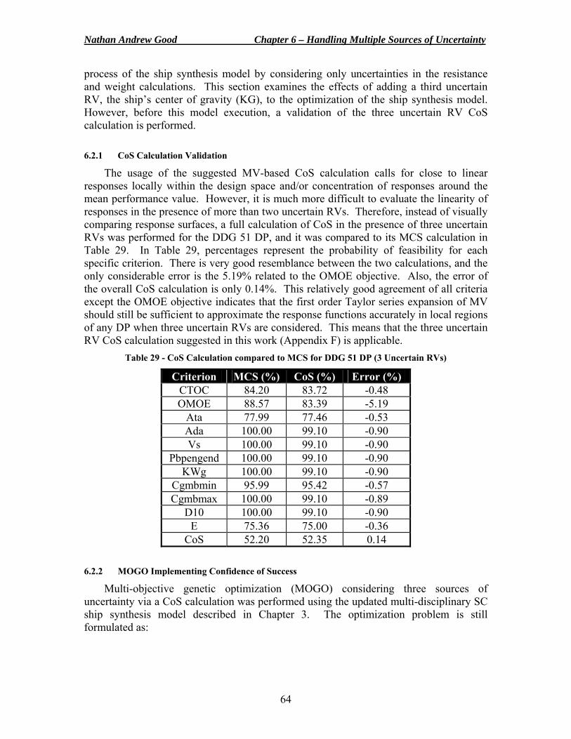
Nathan Andrew Good Chapter 6 – Handling Multiple Sources of Uncertainty
64
process of the ship synthesis model by considering only uncertainties in the resistance and weight calculations. This section examines the effects of adding a third uncertain RV, the ship’s center of gravity (KG), to the optimization of the ship synthesis model. However, before this model execution, a validation of the three uncertain RV CoS calculation is performed. 6.2.1 CoS Calculation Validation
The usage of the suggested MV-based CoS calculation calls for close to linear responses locally within the design space and/or concentration of responses around the mean performance value. However, it is much more difficult to evaluate the linearity of responses in the presence of more than two uncertain RVs. Therefore, instead of visually comparing response surfaces, a full calculation of CoS in the presence of three uncertain RVs was performed for the DDG 51 DP, and it was compared to its MCS calculation in Table 29. In Table 29, percentages represent the probability of feasibility for each specific criterion. There is very good resemblance between the two calculations, and the only considerable error is the 5.19% related to the OMOE objective. Also, the error of the overall CoS calculation is only 0.14%. This relatively good agreement of all criteria except the OMOE objective indicates that the first order Taylor series expansion of MV should still be sufficient to approximate the response functions accurately in local regions of any DP when three uncertain RVs are considered. This means that the three uncertain RV CoS calculation suggested in this work (Appendix F) is applicable.
Table 29 - CoS Calculation compared to MCS for DDG 51 DP (3 Uncertain RVs)
Criterion MCS (%) CoS (%) Error (%) CTOC 84.20 83.72 -0.48 OMOE 88.57 83.39 -5.19
Ata 77.99 77.46 -0.53 Ada 100.00 99.10 -0.90 Vs 100.00 99.10 -0.90
Pbpengend 100.00 99.10 -0.90 KWg 100.00 99.10 -0.90
Cgmbmin 95.99 95.42 -0.57 Cgmbmax 100.00 99.10 -0.89
D10 100.00 99.10 -0.90 E 75.36 75.00 -0.36
CoS 52.20 52.35 0.14 6.2.2 MOGO Implementing Confidence of Success
Multi-objective genetic optimization (MOGO) considering three sources of uncertainty via a CoS calculation was performed using the updated multi-disciplinary SC ship synthesis model described in Chapter 3. The optimization problem is still formulated as:
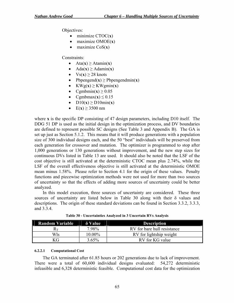
Nathan Andrew Good Chapter 6 – Handling Multiple Sources of Uncertainty
65
Objectives: • minimize CTOC(x) • maximize OMOE(x) • maximize CoS(x)
Constraints:
• Ata(x) ≥ Atamin(x) • Ada(x) ≥ Adamin(x) • Vs(x) ≥ 28 knots • Pbpengend(x) ≥ Pbpengendmin(x) • KWg(x) ≥ KWgmin(x) • Cgmbmin(x) ≥ 0.05 • Cgmbmax(x) ≤ 0.15 • D10(x) ≥ D10min(x) • E(x) ≥ 3500 nm
where x is the specific DP consisting of 47 design parameters, including D10 itself. The DDG 51 DP is used as the initial design in the optimization process, and DV boundaries are defined to represent possible SC designs (See Table 3 and Appendix B). The GA is set up just as Section 5.1.2. This means that it will produce generations with a population size of 300 individual designs each, and the 50 “best” individuals will be preserved from each generation for crossover and mutation. The optimizer is programmed to stop after 1,000 generations or 130 generations without improvement, and the new step sizes for continuous DVs listed in Table 13 are used. It should also be noted that the LSF of the cost objective is still activated at the deterministic CTOC mean plus 2.74%, while the LSF of the overall effectiveness objective is still activated at the deterministic OMOE mean minus 1.58%. Please refer to Section 4.1 for the origin of these values. Penalty functions and piecewise optimization methods were not used for more than two sources of uncertainty so that the effects of adding more sources of uncertainty could be better analyzed.
In this model execution, three sources of uncertainty are considered. These three sources of uncertainty are listed below in Table 30 along with their δ values and descriptions. The origin of these standard deviations can be found in Section 3.3.2, 3.3.3, and 3.3.4.
Table 30 - Uncertainties Analyzed in 3 Uncertain RVs Analysis
Random Variable δ Value Description RT 7.98% RV for bare hull resistance
Wls 10.00% RV for lightship weight KG 3.65% RV for KG value
6.2.2.1 Computational Cost
The GA terminated after 61.85 hours or 202 generations due to lack of improvement. There were a total of 60,600 individual designs evaluated: 54,272 deterministic infeasible and 6,328 deterministic feasible. Computational cost data for the optimization
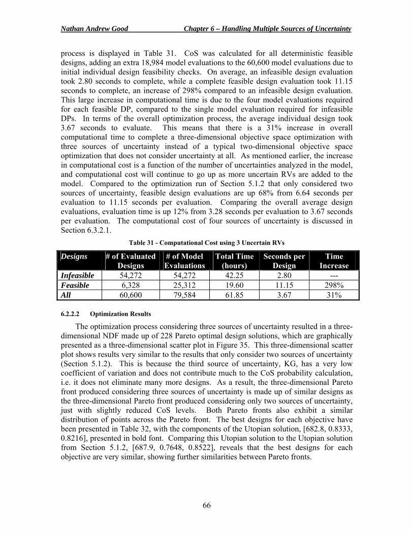
Nathan Andrew Good Chapter 6 – Handling Multiple Sources of Uncertainty
66
process is displayed in Table 31. CoS was calculated for all deterministic feasible designs, adding an extra 18,984 model evaluations to the 60,600 model evaluations due to initial individual design feasibility checks. On average, an infeasible design evaluation took 2.80 seconds to complete, while a complete feasible design evaluation took 11.15 seconds to complete, an increase of 298% compared to an infeasible design evaluation. This large increase in computational time is due to the four model evaluations required for each feasible DP, compared to the single model evaluation required for infeasible DPs. In terms of the overall optimization process, the average individual design took 3.67 seconds to evaluate. This means that there is a 31% increase in overall computational time to complete a three-dimensional objective space optimization with three sources of uncertainty instead of a typical two-dimensional objective space optimization that does not consider uncertainty at all. As mentioned earlier, the increase in computational cost is a function of the number of uncertainties analyzed in the model, and computational cost will continue to go up as more uncertain RVs are added to the model. Compared to the optimization run of Section 5.1.2 that only considered two sources of uncertainty, feasible design evaluations are up 68% from 6.64 seconds per evaluation to 11.15 seconds per evaluation. Comparing the overall average design evaluations, evaluation time is up 12% from 3.28 seconds per evaluation to 3.67 seconds per evaluation. The computational cost of four sources of uncertainty is discussed in Section 6.3.2.1.
Table 31 - Computational Cost using 3 Uncertain RVs
Designs # of Evaluated Designs
# of Model Evaluations
Total Time (hours)
Seconds per Design
Time Increase
Infeasible 54,272 54,272 42.25 2.80 --- Feasible 6,328 25,312 19.60 11.15 298% All 60,600 79,584 61.85 3.67 31% 6.2.2.2 Optimization Results
The optimization process considering three sources of uncertainty resulted in a three-dimensional NDF made up of 228 Pareto optimal design solutions, which are graphically presented as a three-dimensional scatter plot in Figure 35. This three-dimensional scatter plot shows results very similar to the results that only consider two sources of uncertainty (Section 5.1.2). This is because the third source of uncertainty, KG, has a very low coefficient of variation and does not contribute much to the CoS probability calculation, i.e. it does not eliminate many more designs. As a result, the three-dimensional Pareto front produced considering three sources of uncertainty is made up of similar designs as the three-dimensional Pareto front produced considering only two sources of uncertainty, just with slightly reduced CoS levels. Both Pareto fronts also exhibit a similar distribution of points across the Pareto front. The best designs for each objective have been presented in Table 32, with the components of the Utopian solution, [682.8, 0.8333, 0.8216], presented in bold font. Comparing this Utopian solution to the Utopian solution from Section 5.1.2, [687.9, 0.7648, 0.8522], reveals that the best designs for each objective are very similar, showing further similarities between Pareto fronts.
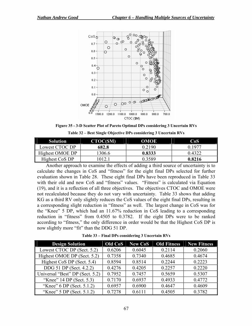
Nathan Andrew Good Chapter 6 – Handling Multiple Sources of Uncertainty
67
Figure 35 - 3-D Scatter Plot of Pareto Optimal DPs considering 3 Uncertain RVs
Table 32 – Best Single Objective DPs considering 3 Uncertain RVs
Solution CTOC($M) OMOE CoS Lowest CTOC DP 682.8 0.2190 0.1977 Highest OMOE DP 1306.6 0.8333 0.4322
Highest CoS DP 1012.1 0.3589 0.8216 Another approach to examine the effects of adding a third source of uncertainty is to
calculate the changes in CoS and “fitness” for the eight final DPs selected for further evaluation shown in Table 28. These eight final DPs have been reproduced in Table 33 with their old and new CoS and “fitness” values. “Fitness” is calculated via Equation (19), and it is a reflection of all three objectives. The objectives CTOC and OMOE were not recalculated because they do not vary with uncertainty. Table 33 shows that adding KG as a third RV only slightly reduces the CoS values of the eight final DPs, resulting in a corresponding slight reduction in “fitness” as well. The largest change in CoS was for the “Knee” 5 DP, which had an 11.67% reduction in CoS leading to a corresponding reduction in “fitness” from 0.4505 to 0.3782. If the eight DPs were to be ranked according to “fitness,” the only difference in order would be that the Highest CoS DP is now slightly more “fit” than the DDG 51 DP.
Table 33 – Final DPs considering 3 Uncertain RVs
Design Solution Old CoS New CoS Old Fitness New Fitness Lowest CTOC DP (Sect. 5.2) 0.6206 0.6045 0.2114 0.2060 Highest OMOE DP (Sect. 5.2) 0.7358 0.7340 0.4685 0.4674
Highest CoS DP (Sect. 5.4) 0.8594 0.8514 0.2244 0.2223 DDG 51 DP (Sect. 4.2.2) 0.4276 0.4205 0.2257 0.2220
Universal “Best” DP (Sect. 5.2) 0.7952 0.7457 0.5659 0.5307 “Knee” 14 DP (Sect. 5.3) 0.7170 0.6937 0.4933 0.4772 “Knee” 6 DP (Sect. 5.1.2) 0.6957 0.6900 0.4647 0.4609 “Knee” 5 DP (Sect. 5.1.2) 0.7278 0.6111 0.4505 0.3782
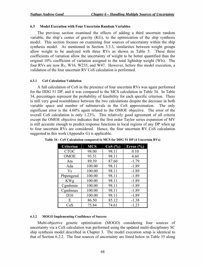
Nathan Andrew Good Chapter 6 – Handling Multiple Sources of Uncertainty
68
6.3 Model Execution with Four Uncertain Random Variables
The previous section examined the effects of adding a third uncertain random variable, the ship’s center of gravity (KG), to the optimization of the ship synthesis model. This section focuses on examining four sources of uncertainty within the ship synthesis model. As mentioned in Section 3.3.3, similarities between weight groups allow weight to be analyzed with three RVs as shown in Table 5. These three coefficients of variation allow the uncertainty of weight to be better quantified than the original 10% coefficient of variation assigned to the total lightship weight (Wls). The four RVs are now RT, W16, W235, and W47. However, before this model execution, a validation of the four uncertain RV CoS calculation is performed. 6.3.1 CoS Calculation Validation
A full calculation of CoS in the presence of four uncertain RVs was again performed for the DDG 51 DP, and it was compared to the MCS calculation in Table 34. In Table 34, percentages represent the probability of feasibility for each specific criterion. There is still very good resemblance between the two calculations despite the decrease in both variable space and number of subintervals in the CoS approximation. The only significant error is the 4.60% again related to the OMOE objective. The error of the overall CoS calculation is only 1.23%. This relatively good agreement of all criteria except the OMOE objective indicates that the first order Taylor series expansion of MV is still accurate enough to predict response functions in local regions of any DP when up to four uncertain RVs are considered. Hence, the four uncertain RV CoS calculation suggested in this work (Appendix G) is applicable.
Table 34 - CoS Calculation compared to MCS for DDG 51 DP (4 Uncertain RVs)
Criterion MCS CoS (%) Error (%) CTOC 98.00 98.11 0.10 OMOE 93.51 98.11 4.60
Ata 89.39 87.60 -1.79 Ada 100.00 98.11 -1.89 Vs 100.00 98.11 -1.89
Pbpengend 100.00 98.11 -1.89 KWg 100.00 98.11 -1.89
Cgmbmin 100.00 98.11 -1.89 Cgmbmax 100.00 98.11 -1.89
D10 100.00 98.11 -1.89 E 86.50 85.12 -1.38
CoS 75.84 74.61 -1.23 6.3.2 MOGO Implementing Confidence of Success
Multi-objective genetic optimization (MOGO) considering four sources of uncertainty via a CoS calculation was performed using the updated multi-disciplinary SC ship synthesis model described in Chapter 3. The model execution setup is identical to that of Section 6.2.2. The four sources of uncertainty are listed below in Table 35 along
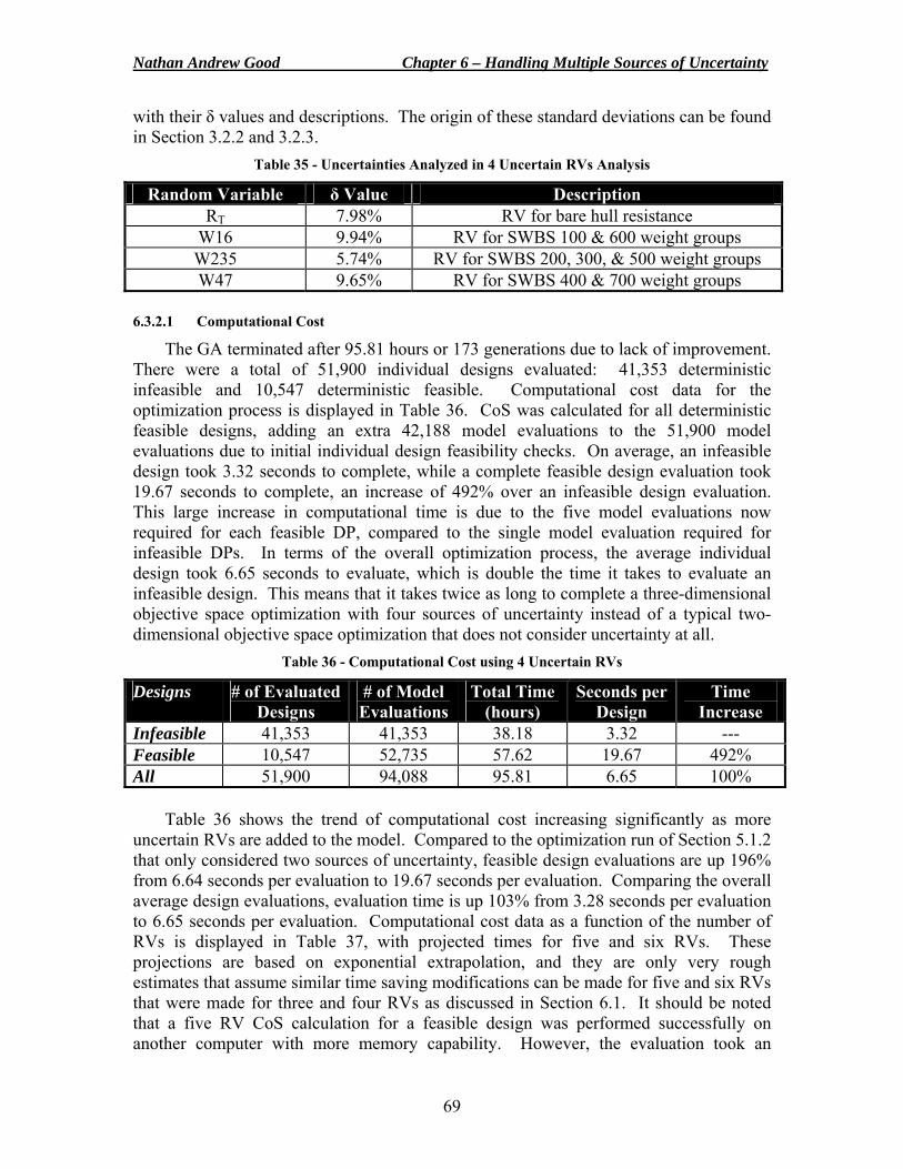
Nathan Andrew Good Chapter 6 – Handling Multiple Sources of Uncertainty
69
with their δ values and descriptions. The origin of these standard deviations can be found in Section 3.2.2 and 3.2.3.
Table 35 - Uncertainties Analyzed in 4 Uncertain RVs Analysis
Random Variable δ Value Description RT 7.98% RV for bare hull resistance
W16 9.94% RV for SWBS 100 & 600 weight groups W235 5.74% RV for SWBS 200, 300, & 500 weight groups W47 9.65% RV for SWBS 400 & 700 weight groups
6.3.2.1 Computational Cost
The GA terminated after 95.81 hours or 173 generations due to lack of improvement. There were a total of 51,900 individual designs evaluated: 41,353 deterministic infeasible and 10,547 deterministic feasible. Computational cost data for the optimization process is displayed in Table 36. CoS was calculated for all deterministic feasible designs, adding an extra 42,188 model evaluations to the 51,900 model evaluations due to initial individual design feasibility checks. On average, an infeasible design took 3.32 seconds to complete, while a complete feasible design evaluation took 19.67 seconds to complete, an increase of 492% over an infeasible design evaluation. This large increase in computational time is due to the five model evaluations now required for each feasible DP, compared to the single model evaluation required for infeasible DPs. In terms of the overall optimization process, the average individual design took 6.65 seconds to evaluate, which is double the time it takes to evaluate an infeasible design. This means that it takes twice as long to complete a three-dimensional objective space optimization with four sources of uncertainty instead of a typical two-dimensional objective space optimization that does not consider uncertainty at all.
Table 36 - Computational Cost using 4 Uncertain RVs
Designs # of Evaluated Designs
# of Model Evaluations
Total Time (hours)
Seconds per Design
Time Increase
Infeasible 41,353 41,353 38.18 3.32 --- Feasible 10,547 52,735 57.62 19.67 492% All 51,900 94,088 95.81 6.65 100%
Table 36 shows the trend of computational cost increasing significantly as more uncertain RVs are added to the model. Compared to the optimization run of Section 5.1.2 that only considered two sources of uncertainty, feasible design evaluations are up 196% from 6.64 seconds per evaluation to 19.67 seconds per evaluation. Comparing the overall average design evaluations, evaluation time is up 103% from 3.28 seconds per evaluation to 6.65 seconds per evaluation. Computational cost data as a function of the number of RVs is displayed in Table 37, with projected times for five and six RVs. These projections are based on exponential extrapolation, and they are only very rough estimates that assume similar time saving modifications can be made for five and six RVs that were made for three and four RVs as discussed in Section 6.1. It should be noted that a five RV CoS calculation for a feasible design was performed successfully on another computer with more memory capability. However, the evaluation took an
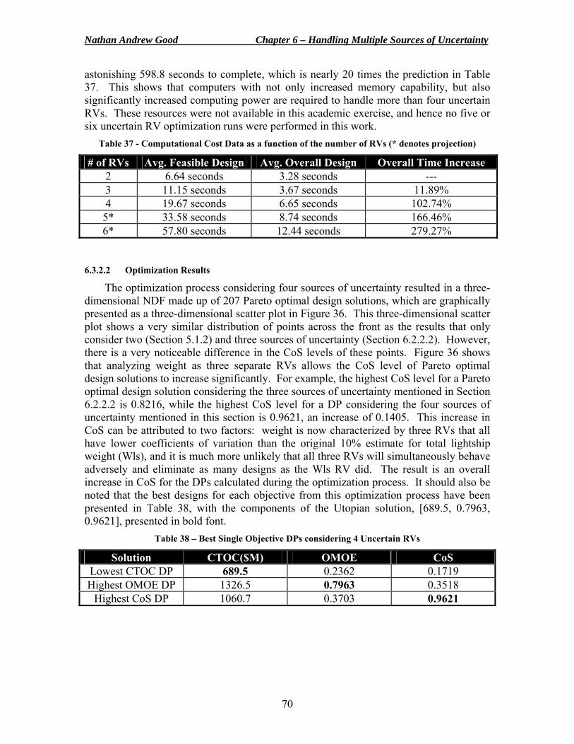
Nathan Andrew Good Chapter 6 – Handling Multiple Sources of Uncertainty
70
astonishing 598.8 seconds to complete, which is nearly 20 times the prediction in Table 37. This shows that computers with not only increased memory capability, but also significantly increased computing power are required to handle more than four uncertain RVs. These resources were not available in this academic exercise, and hence no five or six uncertain RV optimization runs were performed in this work.
Table 37 - Computational Cost Data as a function of the number of RVs (* denotes projection)
# of RVs Avg. Feasible Design Avg. Overall Design Overall Time Increase 2 6.64 seconds 3.28 seconds --- 3 11.15 seconds 3.67 seconds 11.89% 4 19.67 seconds 6.65 seconds 102.74% 5* 33.58 seconds 8.74 seconds 166.46% 6* 57.80 seconds 12.44 seconds 279.27%
6.3.2.2 Optimization Results
The optimization process considering four sources of uncertainty resulted in a three-dimensional NDF made up of 207 Pareto optimal design solutions, which are graphically presented as a three-dimensional scatter plot in Figure 36. This three-dimensional scatter plot shows a very similar distribution of points across the front as the results that only consider two (Section 5.1.2) and three sources of uncertainty (Section 6.2.2.2). However, there is a very noticeable difference in the CoS levels of these points. Figure 36 shows that analyzing weight as three separate RVs allows the CoS level of Pareto optimal design solutions to increase significantly. For example, the highest CoS level for a Pareto optimal design solution considering the three sources of uncertainty mentioned in Section 6.2.2.2 is 0.8216, while the highest CoS level for a DP considering the four sources of uncertainty mentioned in this section is 0.9621, an increase of 0.1405. This increase in CoS can be attributed to two factors: weight is now characterized by three RVs that all have lower coefficients of variation than the original 10% estimate for total lightship weight (Wls), and it is much more unlikely that all three RVs will simultaneously behave adversely and eliminate as many designs as the Wls RV did. The result is an overall increase in CoS for the DPs calculated during the optimization process. It should also be noted that the best designs for each objective from this optimization process have been presented in Table 38, with the components of the Utopian solution, [689.5, 0.7963, 0.9621], presented in bold font.
Table 38 – Best Single Objective DPs considering 4 Uncertain RVs
Solution CTOC($M) OMOE CoS Lowest CTOC DP 689.5 0.2362 0.1719 Highest OMOE DP 1326.5 0.7963 0.3518
Highest CoS DP 1060.7 0.3703 0.9621
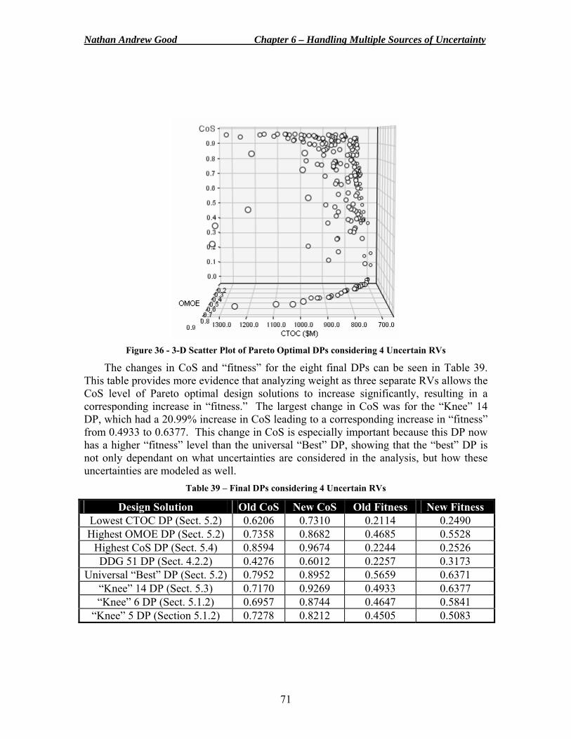
Nathan Andrew Good Chapter 6 – Handling Multiple Sources of Uncertainty
71
Figure 36 - 3-D Scatter Plot of Pareto Optimal DPs considering 4 Uncertain RVs
The changes in CoS and “fitness” for the eight final DPs can be seen in Table 39. This table provides more evidence that analyzing weight as three separate RVs allows the CoS level of Pareto optimal design solutions to increase significantly, resulting in a corresponding increase in “fitness.” The largest change in CoS was for the “Knee” 14 DP, which had a 20.99% increase in CoS leading to a corresponding increase in “fitness” from 0.4933 to 0.6377. This change in CoS is especially important because this DP now has a higher “fitness” level than the universal “Best” DP, showing that the “best” DP is not only dependant on what uncertainties are considered in the analysis, but how these uncertainties are modeled as well.
Table 39 – Final DPs considering 4 Uncertain RVs
Design Solution Old CoS New CoS Old Fitness New Fitness Lowest CTOC DP (Sect. 5.2) 0.6206 0.7310 0.2114 0.2490 Highest OMOE DP (Sect. 5.2) 0.7358 0.8682 0.4685 0.5528
Highest CoS DP (Sect. 5.4) 0.8594 0.9674 0.2244 0.2526 DDG 51 DP (Sect. 4.2.2) 0.4276 0.6012 0.2257 0.3173
Universal “Best” DP (Sect. 5.2) 0.7952 0.8952 0.5659 0.6371 “Knee” 14 DP (Sect. 5.3) 0.7170 0.9269 0.4933 0.6377 “Knee” 6 DP (Sect. 5.1.2) 0.6957 0.8744 0.4647 0.5841
“Knee” 5 DP (Section 5.1.2) 0.7278 0.8212 0.4505 0.5083
Nathan Andrew Good Chapter 6 – Handling Multiple Sources of Uncertainty
72
6.4 Model Execution with Four Uncertain Random Variables Revisited
The previous section examined the effects of analyzing RT, W16, W235, and W47 as uncertain random variables in the optimization of the ship synthesis model. However, as mentioned in Section 3.3.4, there are other critical sources of uncertainty that have yet to be analyzed. This section briefly discusses the effects of considering different combinations of four uncertain RVs in the optimization of the ship synthesis model. 6.4.1 Considering RT, Wls, KG, and KWmflm
MOGO considering four different sources of uncertainty via a CoS calculation was performed using the updated multi-disciplinary SC ship synthesis model of Chapter 3. The model execution setup is still identical to that of Section 6.2.2, only there are four different sources of uncertainty, which are listed below in Table 40 along with their δ values and descriptions. The origin of these standard deviations can be found in Section 3.3.2, 3.3.3, and 3.3.4.
Table 40 - Uncertainties Analyzed in New 4 Uncertain RVs Analysis
Random Variable δ Value Description RT 7.98% RV for bare hull resistance
Wls 10.00% RV for lightship weight KG 3.65% RV for KG value
KWmflm 13.20% RV for maximum functional load with margins
The GA terminated after 61.21 hours or 185 generations due to lack of improvement. The result of the optimization process considering these four sources of uncertainty was the three-dimensional NDF made up of 187 Pareto optimal design solutions, which are graphically presented as a three-dimensional scatter plot in Figure 37. There are no real obvious differences between the shape of this Pareto front and the fronts displayed in Section 5.1.2 and Section 6.2.2.2; therefore, the changes in CoS and “fitness” were again calculated for the eight final DPs to analyze the effects of the four different sources of uncertainty. These results are displayed in Table 41. This table provides evidence that analyzing this set of RVs results in a varying decrease in CoS levels of Pareto optimal design solutions, resulting in a corresponding decrease in “fitness.” The largest change in CoS was for the “Knee” 5 DP, which had a 12.12% decrease in CoS leading to a corresponding decrease in “fitness” from 0.4505 to 0.3755. In contrast, the “Knee” 14 DP only had a 0.70% decrease in CoS, resulting in a very small reduction in “fitness.” These varying degrees of reduction in CoS are a result of which constraint LSFs are active. If the minimum or maximum GM/B ratio constraint (Cgmbmin and Cgmbmax – See Table 4) or generator electric power constraint (KWg – See Table 4) is active, adding KG and KWmflm as RVs will have more of an effect on the CoS calculation, i.e. more designs will be eliminated. However, if these constraints are not active, the effects of adding KG and KWmflm as RVs will be minimal. It is interesting to note that these new sources of uncertainty have adversely affected the DDG51 DP in such a way that it now has the lowest “fitness” level among the final DPs.
Nathan Andrew Good Chapter 6 – Handling Multiple Sources of Uncertainty
73
Figure 37 - 3-D Scatter Plot of Pareto Optimal DPs considering 4 different RVs
Table 41 – Final DPs considering 4 Different Uncertain RVs
Design Solution Old CoS New CoS Old Fitness New FitnessLowest CTOC DP (Sect. 5.2) 0.6206 0.5919 0.2114 0.2016 Highest OMOE DP (Sect. 5.2) 0.7358 0.7175 0.4685 0.4568
Highest CoS DP (Sect. 5.4) 0.8594 0.8506 0.2244 0.2221 DDG 51 DP (Sect. 4.2.2) 0.4276 0.3362 0.2257 0.1775
Universal “Best” DP (Sect. 5.2) 0.7952 0.7359 0.5659 0.5237 “Knee” 14 DP (Sect. 5.3) 0.7170 0.7100 0.4933 0.4885 “Knee” 6 DP (Sect. 5.1.2) 0.6957 0.6833 0.4647 0.4564 “Knee” 5 DP (Sect. 5.1.2) 0.7278 0.6066 0.4505 0.3755
6.4.2 Considering RT, Wls, Atr, and E
MOGO considering a new set of four RVs was performed using the updated multi-disciplinary SC ship synthesis model of Chapter 3. The model execution setup is still identical to that of Section 6.2.2.2, only there are again four different sources of uncertainty, which are listed below in Table 42 along with their δ values and descriptions. Bare hull resistance (RT) and lightship weight (Wls) remain as sources of uncertainty because they are the two most significant sources of uncertainty in the ship synthesis analyses.
Table 42 - Uncertainties Analyzed in New 4 Uncertain RVs Analysis
Random Variable δ Value Description RT 7.98% RV for bare hull resistance
Wls 10.00% RV for lightship weight Atr 10.00% RV for total required area E 10.00% RV for endurance range
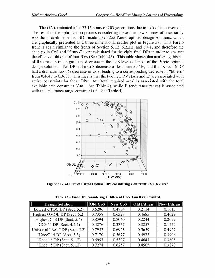
Nathan Andrew Good Chapter 6 – Handling Multiple Sources of Uncertainty
74
The GA terminated after 73.15 hours or 203 generations due to lack of improvement. The result of the optimization process considering these four new sources of uncertainty was the three-dimensional NDF made up of 252 Pareto optimal design solutions, which are graphically presented as a three-dimensional scatter plot in Figure 38. This Pareto front is again similar to the fronts of Section 5.1.2, 6.2.2.2, and 6.4.1, and therefore the changes in CoS and “fitness” were calculated for the eight final DPs in order to analyze the effects of this set of four RVs (See Table 43). This table shows that analyzing this set of RVs results in a significant decrease in the CoS levels of most of the Pareto optimal design solutions. No DP had a CoS decrease of less than 5.54%, and the “Knee” 6 DP had a dramatic 15.60% decrease in CoS, leading to a corresponding decrease in “fitness” from 0.4647 to 0.3605. This means that the two new RVs (Atr and E) are associated with active constraints for these DPs: Atr (total required area) is associated with the total available area constraint (Ata – See Table 4), while E (endurance range) is associated with the endurance range constraint (E – See Table 4).
Figure 38 - 3-D Plot of Pareto Optimal DPs considering 4 different RVs Revisited
Table 43 – Final DPs considering 4 Different Uncertain RVs Revisited
Design Solution Old CoS New CoS Old Fitness New FitnessLowest CTOC DP (Sect. 5.2) 0.6206 0.4734 0.2114 0.1613 Highest OMOE DP (Sect. 5.2) 0.7358 0.6327 0.4685 0.4029
Highest CoS DP (Sect. 5.4) 0.8594 0.8040 0.2244 0.2099 DDG 51 DP (Sect. 4.2.2) 0.4276 0.3357 0.2257 0.1772
Universal “Best” DP (Sect. 5.2) 0.7952 0.6923 0.5659 0.4927 “Knee” 14 DP (Sect. 5.3) 0.7170 0.5677 0.4933 0.3906 “Knee” 6 DP (Sect. 5.1.2) 0.6957 0.5397 0.4647 0.3605 “Knee” 5 DP (Sect. 5.1.2) 0.7278 0.6257 0.4505 0.3873
Nathan Andrew Good Chapter 6 – Handling Multiple Sources of Uncertainty
75
6.5 Overall Observations
There are many critical sources of uncertainty embedded within the ship synthesis model, and all of these uncertainties need to be realistically quantified and represented in the model in order to investigate the true overall design uncertainty. In this work, only a handful of parameters that directly affect the CTOC and OMOE objectives and nine design constraints were identified as sources of uncertainty in an effort to approximate the overall design uncertainty. This Chapter focused on analyzing more than two of these uncertainties at a time, and it was shown that a maximum of four sources of uncertainty could be handled by the current CoS calculation. If more than four sources of uncertainty need to be analyzed at once, a significant upgrade in computing power and computer memory is required. This makes the selection of uncertainties in the optimization process critical to the results. The “best” DPs are a direct reflection of which uncertainties are considered in the analysis, as well as how these uncertainties are modeled. For example, the results of this Chapter show Pareto fronts that are dependant on the selection and modeling of uncertainties. Also, some of the attractive designs from Chapter 5 are no longer attractive in Chapter 6 because new uncertainties have revealed other active constraints that endanger the DPs of not satisfying constraints and/or not meeting performance objectives. Therefore, only designs that exhibit high “fitness” levels for any combination of uncertainty analyses should be considered as potential baseline designs. Other designs are not reliable enough to satisfy all constraints and meet performance objectives concurrently.
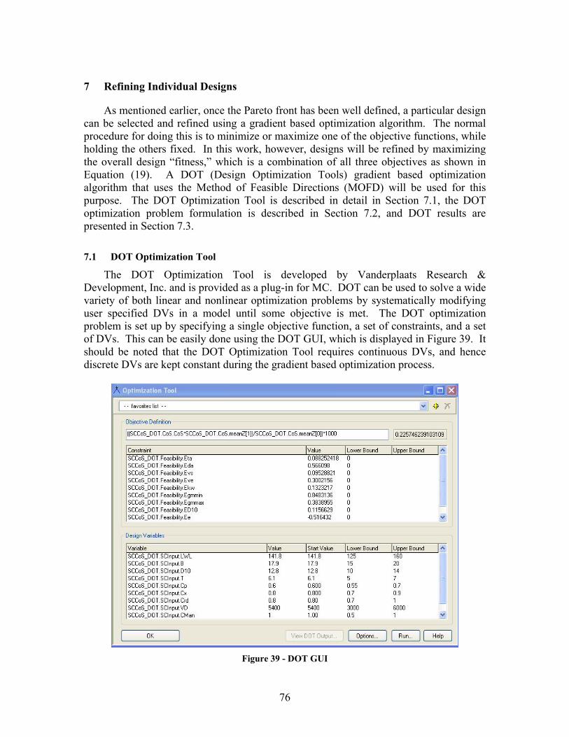
76
7 Refining Individual Designs
As mentioned earlier, once the Pareto front has been well defined, a particular design can be selected and refined using a gradient based optimization algorithm. The normal procedure for doing this is to minimize or maximize one of the objective functions, while holding the others fixed. In this work, however, designs will be refined by maximizing the overall design “fitness,” which is a combination of all three objectives as shown in Equation (19). A DOT (Design Optimization Tools) gradient based optimization algorithm that uses the Method of Feasible Directions (MOFD) will be used for this purpose. The DOT Optimization Tool is described in detail in Section 7.1, the DOT optimization problem formulation is described in Section 7.2, and DOT results are presented in Section 7.3. 7.1 DOT Optimization Tool
The DOT Optimization Tool is developed by Vanderplaats Research & Development, Inc. and is provided as a plug-in for MC. DOT can be used to solve a wide variety of both linear and nonlinear optimization problems by systematically modifying user specified DVs in a model until some objective is met. The DOT optimization problem is set up by specifying a single objective function, a set of constraints, and a set of DVs. This can be easily done using the DOT GUI, which is displayed in Figure 39. It should be noted that the DOT Optimization Tool requires continuous DVs, and hence discrete DVs are kept constant during the gradient based optimization process.
Figure 39 - DOT GUI
Nathan Andrew Good Chapter 7 – Refining Individual Designs
77
The DOT Optimization Tool supports a variety of different optimization methods
and settings. The optimization methods offered include: 1) Variable Metric Method 2) Conjugate Gradient Method 3) Method of Feasible Directions 4) Sequential Linear Programming 5) Sequential Quadratic Programming
The first two of these optimization methods are applicable when no constraints are specified, while the last three optimization methods are applicable when constraints are specified. The Method of Feasible Directions (MOFD) optimization technique is used in this work. The basic approach of MOFD is to solve the optimization problem in two distinct steps. The first step is to determine a “search direction” which defines how the DVs will be changed. The key idea is that all DVs are changed simultaneously in such a fashion that will improve the design. The second step is to determine how far to move in the “search direction.” After moving this distance in the “search direction,” the process is repeated until it converges to the optimum (Vanderplaats, 1995). In general, the optimizer will run the model several times to calculate gradients and then compute the step direction. Each step represents one iteration or optimization run. Optimization convergence is controlled by several parameters, including maximum iterations, absolute convergence criteria, and relative convergence criteria. For more information concerning the DOT Optimization Tool, please visit http://www.phoenix-int.com/ or http://www.vrand.com/DOT.html. 7.2 DOT Optimization Problem Formulation
Gradient based optimization was performed on the eight final DPs selected for further evaluation (See Table 28) using the DOT Optimization Tool in an effort to refine the DPs and increase objective values. In this work, designs are refined by maximizing the overall design “fitness,” which is a combination of all three objectives as shown in Equation (19). The optimization problem is now formulated as: Objective:
• maximize Fitness(x)
Constraints: • Ata(x) ≥ Atamin(x) • Ada(x) ≥ Adamin(x) • Vs(x) ≥ 28 knots • Pbpengend(x) ≥ Pbpengendmin(x) • KWg(x) ≥ KWgmin(x) • Cgmbmin(x) ≥ 0.05 • Cgmbmax(x) ≤ 0.15 • D10(x) ≥ D10min(x) • E(x) ≥ 3500 nm
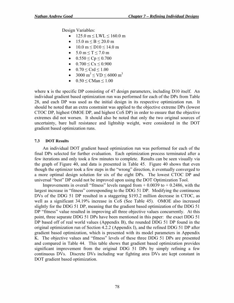
Nathan Andrew Good Chapter 7 – Refining Individual Designs
78
Design Variables: • 125.0 m ≤ LWL ≤ 160.0 m • 15.0 m ≤ B ≤ 20.0 m • 10.0 m ≤ D10 ≤ 14.0 m • 5.0 m ≤ T ≤ 7.0 m • 0.550 ≤ Cp ≤ 0.700 • 0.700 ≤ Cx ≤ 0.900 • 0.70 ≤ Crd ≤ 1.00 • 3000 m3 ≤ VD ≤ 6000 m3 • 0.50 ≤ CMan ≤ 1.00
where x is the specific DP consisting of 47 design parameters, including D10 itself. An individual gradient based optimization run was performed for each of the DPs from Table 28, and each DP was used as the initial design in its respective optimization run. It should be noted that an extra constraint was applied to the objective extreme DPs (lowest CTOC DP, highest OMOE DP, and highest CoS DP) in order to ensure that the objective extremes did not worsen. It should also be noted that only the two original sources of uncertainty, bare hull resistance and lightship weight, were considered in the DOT gradient based optimization runs. 7.3 DOT Results
An individual DOT gradient based optimization run was performed for each of the final DPs selected for further evaluation. Each optimization process terminated after a few iterations and only took a few minutes to complete. Results can be seen visually via the graph of Figure 40, and data is presented in Table 45. Figure 40 shows that even though the optimizer took a few steps in the “wrong” direction, it eventually converged to a more optimal design solution for six of the eight DPs. The lowest CTOC DP and universal “best” DP could not be improved upon using the DOT Optimization Tool.
Improvements in overall “fitness” levels ranged from + 0.0039 to + 0.2486, with the largest increase in “fitness” corresponding to the DDG 51 DP. Modifying the continuous DVs of the DDG 51 DP resulted in a staggering $193.2 million decrease in CTOC, as well as a significant 34.19% increase in CoS (See Table 45). OMOE also increased slightly for the DDG 51 DP, meaning that the gradient based optimization of the DDG 51 DP “fitness” value resulted in improving all three objective values concurrently. At this point, three separate DDG 51 DPs have been mentioned in this paper: the exact DDG 51 DP based off of real world values (Appendix B), the rounded DDG 51 DP found in the original optimization run of Section 4.2.2 (Appendix I), and the refined DDG 51 DP after gradient based optimization, which is presented with its model parameters in Appendix K. The objective values and “fitness” levels of these three DDG 51 DPs are presented and compared in Table 44. This table shows that gradient based optimization provides significant improvement from the original DDG 51 DPs by simply refining a few continuous DVs. Discrete DVs including war fighting area DVs are kept constant in DOT gradient based optimization.
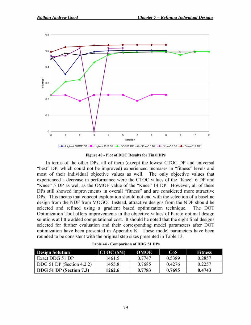
Nathan Andrew Good Chapter 7 – Refining Individual Designs
79
0
0.1
0.2
0.3
0.4
0.5
0.6
0 1 2 3 4 5 6 7 8 9 10 11
Iteration
"Fitn
ess"
Highest OMOE DP Highest CoS DP DDG51 DP "Knee" 5 DP "Knee" 6 DP "Knee" 14 DP Figure 40 - Plot of DOT Results for Final DPs
In terms of the other DPs, all of them (except the lowest CTOC DP and universal “best” DP, which could not be improved) experienced increases in “fitness” levels and most of their individual objective values as well. The only objective values that experienced a decrease in performance were the CTOC values of the “Knee” 6 DP and “Knee” 5 DP as well as the OMOE value of the “Knee” 14 DP. However, all of these DPs still showed improvements in overall “fitness” and are considered more attractive DPs. This means that concept exploration should not end with the selection of a baseline design from the NDF from MOGO. Instead, attractive designs from the NDF should be selected and refined using a gradient based optimization technique. The DOT Optimization Tool offers improvements in the objective values of Pareto optimal design solutions at little added computational cost. It should be noted that the eight final designs selected for further evaluation and their corresponding model parameters after DOT optimization have been presented in Appendix K. These model parameters have been rounded to be consistent with the original step sizes presented in Table 13.
Table 44 - Comparison of DDG 51 DPs
Design Solution CTOC ($M) OMOE CoS Fitness Exact DDG 51 DP 1461.5 0.7747 0.5389 0.2857 DDG 51 DP (Section 4.2.2) 1455.8 0.7685 0.4276 0.2257 DDG 51 DP (Section 7.3) 1262.6 0.7783 0.7695 0.4743
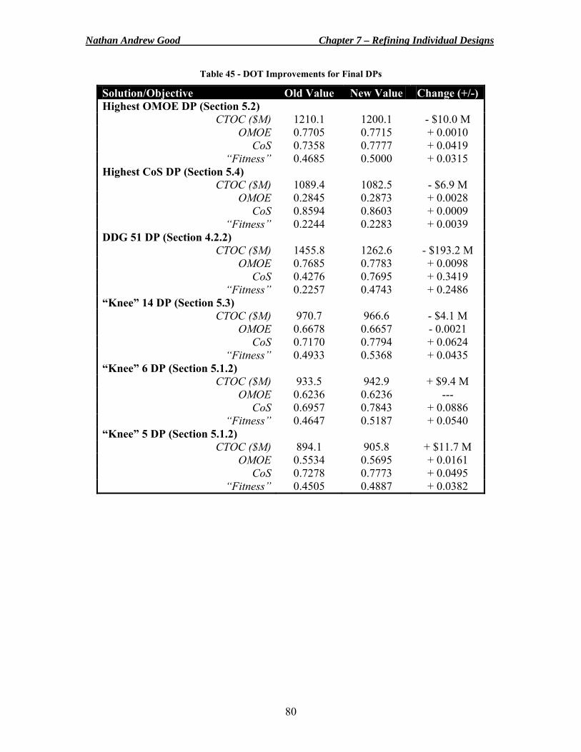
Nathan Andrew Good Chapter 7 – Refining Individual Designs
80
Table 45 - DOT Improvements for Final DPs
Solution/Objective Old Value New Value Change (+/-)Highest OMOE DP (Section 5.2)
CTOC ($M) 1210.1 1200.1 - $10.0 M OMOE 0.7705 0.7715 + 0.0010
CoS 0.7358 0.7777 + 0.0419 “Fitness” 0.4685 0.5000 + 0.0315
Highest CoS DP (Section 5.4) CTOC ($M) 1089.4 1082.5 - $6.9 M
OMOE 0.2845 0.2873 + 0.0028 CoS 0.8594 0.8603 + 0.0009
“Fitness” 0.2244 0.2283 + 0.0039 DDG 51 DP (Section 4.2.2)
CTOC ($M) 1455.8 1262.6 - $193.2 M OMOE 0.7685 0.7783 + 0.0098
CoS 0.4276 0.7695 + 0.3419 “Fitness” 0.2257 0.4743 + 0.2486
“Knee” 14 DP (Section 5.3) CTOC ($M) 970.7 966.6 - $4.1 M
OMOE 0.6678 0.6657 - 0.0021 CoS 0.7170 0.7794 + 0.0624
“Fitness” 0.4933 0.5368 + 0.0435 “Knee” 6 DP (Section 5.1.2)
CTOC ($M) 933.5 942.9 + $9.4 M OMOE 0.6236 0.6236 ---
CoS 0.6957 0.7843 + 0.0886 “Fitness” 0.4647 0.5187 + 0.0540
“Knee” 5 DP (Section 5.1.2) CTOC ($M) 894.1 905.8 + $11.7 M
OMOE 0.5534 0.5695 + 0.0161 CoS 0.7278 0.7773 + 0.0495
“Fitness” 0.4505 0.4887 + 0.0382
81
8 Non-Intrusive Polynomial Chaos (NIPC) Method
The usage of the MV-based CoS calculation suggested in this work calls for close to linear responses locally within the design space and/or concentration of responses around the mean performance value. While the current multi-disciplinary SC ship synthesis model has close to linear responses, there are other highly nonlinear engineering models in need of another method of handling uncertainty propagation. An inexpensive non-intrusive polynomial chaos (NIPC) method for the propagation of input uncertainty in CFD simulations has recently been developed at VT AOE by Hosder, Walters, and Perez (2006). This NIPC method is straightforward to implement and computationally less expensive than sampling or quadrature based non-intrusive methods. The method has been validated through implementation in three basic fluid dynamics problems. In all three test cases, the statistics obtained using the NIPC method were in good agreement with MCS calculated statistics. A fourth order polynomial chaos (PC) expansion was sufficient to approximate the mean, standard deviation, and shape of the output uncertainty distributions with desired accuracy (Hosder et al., 2006). For these reasons, the NIPC method and its application to nonlinear ship synthesis models are briefly discussed in this Chapter.
The PC method for uncertainty propagation in CFD simulations and other computational modeling involves the substitution of uncertain variables and parameters in the governing equations with the polynomial expansions. In general, an intrusive PC method will compute the unknown polynomial coefficients by projecting the resulting equations onto basis functions (orthogonal polynomials) for different modes, which requires the modification of the deterministic code. A more convenient approach is the NIPC method for the propagation of input uncertainty discussed here (Hosder et al., 2006).
In the spectral representation of uncertainty, one may decompose a random function or RV into separable deterministic and stochastic components. For example, any stochastic variable or response (i.e. α*) such as velocity or cost with random fluctuations can be written as:
( ) ( ) ( )∑=
Ψ=P
iii yxyx
0
* ,,, ξαξα (25)
where αi(x,y) is the deterministic component and Ψi(ξ) is the random basis function corresponding to the ith mode. The parameter α* is assumed to be a function of deterministic independent variables x and y, and ξ = (ξ1,…,ξn) is an n-dimensional RV vector with a specific probability distribution. The discrete sum is taken over the number of output modes:
( )!!
!1pnpnP +
=+ (26)
where p is the order of polynomial chaos (we will assume 4) and n is the number of random dimensions (also assumed to be 4). For the basis function, multi-dimensional Hermite polynomials are used to span the n-dimensional random space:
( ) ( ) ⎟⎟⎠
⎞⎜⎜⎝
⎛−=
− ξξξξ
δξδξδξξ
TT
eii
eiiHk
kk
kk21
1
21
1 ...1,..., (27)
Nathan Andrew Good Chapter 8 – Non-Intrusive Polynomial Chaos Method
82
where k = 0, 1, …, p. As mentioned earlier, to model uncertainty propagation in computational simulations via the intrusive PC approach, all dependant variables and random parameters in the governing equations must be replaced with their PC expansions, which can be difficult, expensive, and time consuming to implement. Therefore, an inexpensive NIPC method has been developed for uncertainty propagation within complex engineering systems (Hosder et al., 2006).
The present NIPC method begins by replacing the uncertain variables of interest with their polynomial expansions given by Equation (25). Next, for a given PC of order P, P + 1 vectors ξ = {ξ1,ξ2,…,ξn}i, (i = 0,1,2,…,P) in random space are chosen and the deterministic code is evaluated at these points. With the left hand side of Equation (25) known from the solutions of the deterministic evaluations at the selected random points, a linear system of equations is obtained:
( ) ( ) ( )( ) ( ) ( )
( ) ( ) ( )
( )( )
( )⎟⎟⎟⎟⎟
⎠
⎞
⎜⎜⎜⎜⎜
⎝
⎛
=
⎟⎟⎟⎟⎟
⎠
⎞
⎜⎜⎜⎜⎜
⎝
⎛
⎟⎟⎟⎟⎟
⎠
⎞
⎜⎜⎜⎜⎜
⎝
⎛
ΨΨΨ
ΨΨΨΨΨΨ
pppppp
p
p
ξα
ξαξα
α
αα
ξξξ
ξξξξξξ
…
……
*
1*
0*
1
0
10
11110
00100
(28)
The spectral modes (αk) of the RV, α*, are then obtained by simply solving this linear system of equations. This method is considered “non-intrusive” because no modification to the deterministic code is needed, i.e. the deterministic code is treated like a “black box.” The NIPC method is straightforward to implement, requires one LU decomposition, and requires a minimum of P+1 deterministic evaluations to estimate statistics (Hosder et al., 2006).
Consider the case of the multi-disciplinary ship synthesis model presented in this work. If four sources of uncertainty (n = 4) are analyzed and a fourth order PC expansion is required for accuracy, the number of output modes according to Equation (26) would be 70. This means that 70 deterministic model evaluations would be required to model the response functions of the ship synthesis model. Using the current suggested MV-based CoS calculation, only five deterministic model evaluations would be required to estimate the response functions in the presence of four uncertain RVs. Therefore, for a model with close to linear responses locally within the design space, a MV-based CoS calculation is the much more efficient choice. However, as non-linearities arise in the model, the MV-based CoS calculation becomes less accurate and not applicable, making the NIPC method a possible uncertainty propagation tool for nonlinear engineering systems because of its computational cost savings compared to other methods such as the intrusive PC method or MCS. For more information on the NIPC method, please consult “A Non-Intrusive Polynomial Chaos Method for Uncertainty Propagation in CFD Simulations” (Hosder et al., 2006).
83
9 Conclusions
Multi-disciplinary ship synthesis models and multi-objective genetic algorithms are increasingly being used in naval ship design, allowing a total system approach for the naval ship design process. Complex system design problems such as these often have high levels of uncertainty associated with them, and there is an increasing demand for a decision making tool that accounts for the effects of uncertainties in the design process to produce results that are both effective and reliable. In this work, uncertainty is treated as a third objective in addition to the effectiveness and cost objectives already present in a multi-disciplinary surface combatant ship synthesis model by using a calculation termed “confidence of success” (CoS) based on the mean value method. CoS is the probability that a specific design will satisfy all constraints and meet performance objectives.
This work proves that the CoS concept can be applied to complex system models with well behaved responses to estimate system uncertainty early in the design process. Multiple sources of uncertainty were realistically quantified based on statistical background and represented in a multi-disciplinary surface combatant ship synthesis model developed at VT AOE in order to investigate their relative importance to overall design uncertainty or risk. Combinations of up to four of these sources of uncertainty were successfully implemented in the multi-objective genetic optimization of the ship synthesis model via a mean value method based CoS calculation. Methods to encourage a more uniform distribution of points across the front were also investigated through the discretization of continuous design variables, the modification of optimization parameters, piecewise optimization, and the application of a penalty function. With a well defined front, particular designs were selected and refined using a gradient based optimization algorithm to maximize the overall fitness of each design.
The usage of the suggested CoS calculation calls for close to linear responses locally within the design space and/or concentration of responses around the mean performance value. Therefore, before the initial model execution, an examination of the model response was performed in Chapter 4 for a few deterministically feasible design points via short sample MCS calculations of 100,000 system evaluations each. The relatively well-behaved response surfaces of the CTOC objective and the constraints indicated that the first order Taylor series expansion of the mean value method was sufficient to approximate the response functions accurately in local regions of any design point. Multi-objective genetic optimization considering two sources of uncertainty via a CoS calculation was performed using the updated multi-disciplinary surface combatant ship synthesis model, resulting in a three-dimensional non-dominated frontier made up of 225 Pareto optimal design solutions. However, in this initial optimization effort, the design points did not spread out well over the Pareto front.
Methods to encourage a more uniform distribution of design points across the Pareto front were investigated in Chapter 5. It was found that once the optimization problem is formulated correctly, continuous DVs should be discretized in order to reduce the number of possible designs the optimizer has to search. Optimization parameters should then be adjusted to suit the optimization problem at hand. It was also found that a penalty function or piecewise optimization scheme can be used to significantly enhance these results if the designer is willing to pay more in terms of computational cost. With a well defined Pareto front, attractive designs can be selected from the front for more uncertainty analysis and gradient based optimization.
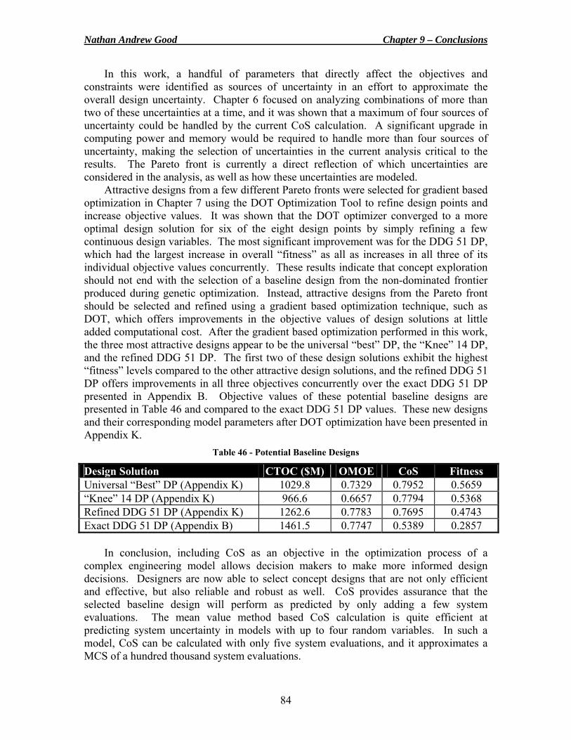
Nathan Andrew Good Chapter 9 – Conclusions
84
In this work, a handful of parameters that directly affect the objectives and constraints were identified as sources of uncertainty in an effort to approximate the overall design uncertainty. Chapter 6 focused on analyzing combinations of more than two of these uncertainties at a time, and it was shown that a maximum of four sources of uncertainty could be handled by the current CoS calculation. A significant upgrade in computing power and memory would be required to handle more than four sources of uncertainty, making the selection of uncertainties in the current analysis critical to the results. The Pareto front is currently a direct reflection of which uncertainties are considered in the analysis, as well as how these uncertainties are modeled.
Attractive designs from a few different Pareto fronts were selected for gradient based optimization in Chapter 7 using the DOT Optimization Tool to refine design points and increase objective values. It was shown that the DOT optimizer converged to a more optimal design solution for six of the eight design points by simply refining a few continuous design variables. The most significant improvement was for the DDG 51 DP, which had the largest increase in overall “fitness” as all as increases in all three of its individual objective values concurrently. These results indicate that concept exploration should not end with the selection of a baseline design from the non-dominated frontier produced during genetic optimization. Instead, attractive designs from the Pareto front should be selected and refined using a gradient based optimization technique, such as DOT, which offers improvements in the objective values of design solutions at little added computational cost. After the gradient based optimization performed in this work, the three most attractive designs appear to be the universal “best” DP, the “Knee” 14 DP, and the refined DDG 51 DP. The first two of these design solutions exhibit the highest “fitness” levels compared to the other attractive design solutions, and the refined DDG 51 DP offers improvements in all three objectives concurrently over the exact DDG 51 DP presented in Appendix B. Objective values of these potential baseline designs are presented in Table 46 and compared to the exact DDG 51 DP values. These new designs and their corresponding model parameters after DOT optimization have been presented in Appendix K.
Table 46 - Potential Baseline Designs
Design Solution CTOC ($M) OMOE CoS Fitness Universal “Best” DP (Appendix K) 1029.8 0.7329 0.7952 0.5659 “Knee” 14 DP (Appendix K) 966.6 0.6657 0.7794 0.5368 Refined DDG 51 DP (Appendix K) 1262.6 0.7783 0.7695 0.4743 Exact DDG 51 DP (Appendix B) 1461.5 0.7747 0.5389 0.2857
In conclusion, including CoS as an objective in the optimization process of a complex engineering model allows decision makers to make more informed design decisions. Designers are now able to select concept designs that are not only efficient and effective, but also reliable and robust as well. CoS provides assurance that the selected baseline design will perform as predicted by only adding a few system evaluations. The mean value method based CoS calculation is quite efficient at predicting system uncertainty in models with up to four random variables. In such a model, CoS can be calculated with only five system evaluations, and it approximates a MCS of a hundred thousand system evaluations.
85
10 Future Work
This work proved that a CoS concept can be applied to complex system models with well behaved responses and up to four sources of uncertainty. Methods to encourage a more uniform distribution of points across the Pareto front were also investigated, and gradient based optimization was performed as well. However, there is still potential future work for the problem of uncertainty propagation in engineering systems.
Most future work lies in the area of uncertainty propagation in highly nonlinear engineering systems. For a model with close to linear responses locally within the design space, a CoS calculation based on a first order Taylor series expansion is very efficient. However, as non-linearities arise in the model, a CoS calculation becomes less accurate and not applicable. Furthermore, a CoS calculation will not reveal that there may be a problem with the approximation of a system response. One potential solution is an extra system evaluation evaluated at the most probable point (MPP) that could identify approximation problems and improve the limit state function (LSF) approximations of all criteria (Klasen, 2005). Another possible uncertainty propagation tool for nonlinear engineering systems is the NIPC method mentioned in this work. The NIPC method requires even more system evaluations, but still offers significant computational cost savings compared to other nonlinear methods such as the intrusive PC method or MCS.
Other work lies in the area of increasing the number of uncertainties analyzed in the optimization process. In this work, only a handful of parameters that directly affect the objectives and constraints were identified as sources of uncertainty. It might be interesting to examine the effects of applying uncertainties to the data called by discrete design variables as well. The CoS calculation is quite efficient at predicting system uncertainty for models with up to four random variables, but it has been shown that computational cost increases significantly as more uncertain random variables are added to the model. More computer memory and computing power will be required for these calculations. Also, the effect of more than four random variables on criteria responses has yet to be explored.
There are other areas of work as well. Since the Taylor series expansion of the mean value method can also be used for sensitivity measures, additional objectives such as criteria variance could be incorporated into the optimization process (Klasen, 2005). A complete sensitivity analysis could also be performed in order to identify the critical design variables in the optimization process. Design variables that have little impact on the results could potentially be removed to significantly reduce the design space. As mentioned earlier, it would also be beneficial if a penalty function were built into the Darwin Optimization plug-in itself. The required inputs for the penalty function could be added to the Darwin Optimization plug-in GUI, and incorporation of the penalty function into the actual genetic algorithm would offer decreased computational time over using a separate penalty function module, as is done in this work. Finally, multi-objective genetic optimization considering uncertainty via a CoS calculation could be performed in conjunction with the ASSET design tool to calculate uncertainty propagation in other modern USN ship design models.
Nathan Andrew Good References
86
References
Benini, Ernesto. “Multiobjective Design Optimization of B-Screw Series Propellers Using Evolutionary Algorithms.” Marine Technology 40.4 (2003): 229-238.
Brown, Alan. “Ship Design Notes.” Virginia Tech AOE Department (2006). Brown, Alan and Mark Thomas. “Reengineering the Naval Ship Concept Design Process.”
ASNE From Research to Reality in Ship Systems Engineering Symposium, Tysons Corner, VA, September 1998.
Doehring, Thoralf. “USS Arleigh Burke (DDG 51).” Unofficial US Navy Site. 2006. <http://navysite.de/dd/ddg51.htm>.
Du, Xiaoping and Wei Chen. “Efficient Uncertainty Analysis Methods for Multidisciplinary Robust Design.” AIAA Journal 40.3 (2002): 545-552.
Good, Nathan, Morgan Baldwin, Aaron Cox, Nick Marickovich, Travis Smith, and Ryan Webster. “Design Report: Advanced Logistics Delivery Ship (ALDV).” 2005 ASNE/SNAME Dr. James A. Lisnyk Ship Design Competition.
Good, Nathan and Alan Brown. “Multi-Objective Concept Design of an Advanced Logistics Delivery System Ship (ALDV).” ASNE Joint Sea Basing Symposium, Arlington, VA, March 2006.
Holtrop, Jan. “A Statistical Re-Analysis of Resistance and Propulsion Data.” International Shipbuilding Progress 31.363 (1984): 272-276.
Hosder, S., R. W. Walters, and R. Perez. “A Non-Intrusive Polynomial Chaos Method for Uncertainty Propagation in CFD Simulations.” AIAA 44th Aerospace Sciences Meeting and Exhibit, Reno, NV, January 2006.
Klasen, Emanuel. “Confidence of Success in Multi-Criteria Optimization of Multi-Disciplinary Ship Design Models.” VPISU Report (2005).
Mavris, D. N., D. A. DeLaurentis, O. Bandte, M. A. Hale. “A Stochastic Approach to Multi-disciplinary Aircraft Analysis and Design.” AIAA 36th Aerospace Sciences Meeting and Exhibit, Reno, NV, January 1998.
Montgomery, Douglas C., George C. Runger, and Norma F. Hubele. Engineering Statistics. 3rd ed. New York: John Wiley & Sons, Inc., 2004.
Southwest Research Institute. NESSUS Theoretical Manual. San Antonio: Southwest Research Institute, 2001.
Stepanchick, Justin and Alan Brown. “Revisiting DDGX/DDG-51 Concept Exploration.” ASNE Day, Arlington, VA, June 2006.
Thacker, Ben H., Daniel P. Nicolella, Srirangam Kumaresan, Narayan Yoganandan, and Frank A. Pintar. “Probabilistic Finite Element Analysis of the Human Lower Cervical Spine.” Journal of Mathematical Modeling and Scientific Computing 13.1-2 (2001): 12-21.
Toppan, Andrew. “World Navies Today: US Navy Aircraft Carriers & Surface Combatants.” Haze Gray & Underway. 10 March 2003. 2006. <http://www.hazegray.org/worldnav/usa/surface.htm>.
Vanderplaats Research & Development, Inc. DOT Users Manual Version 4.20. Colorado Springs: VR&D, 1995.
“What is Monte Carlo Simulation?” Decisioneering. 2005. Decisioneering, Inc. 2006. <http://www.decisioneering.com/monte-carlo-simulation.html>.
Wu, Y. T., H. R. Millwater, and T. A. Cruse. “Advanced Probabilistic Structural Analysis Method for Implicit Performance Functions.” AIAA Journal 28.9 (1990): 1663-1669.
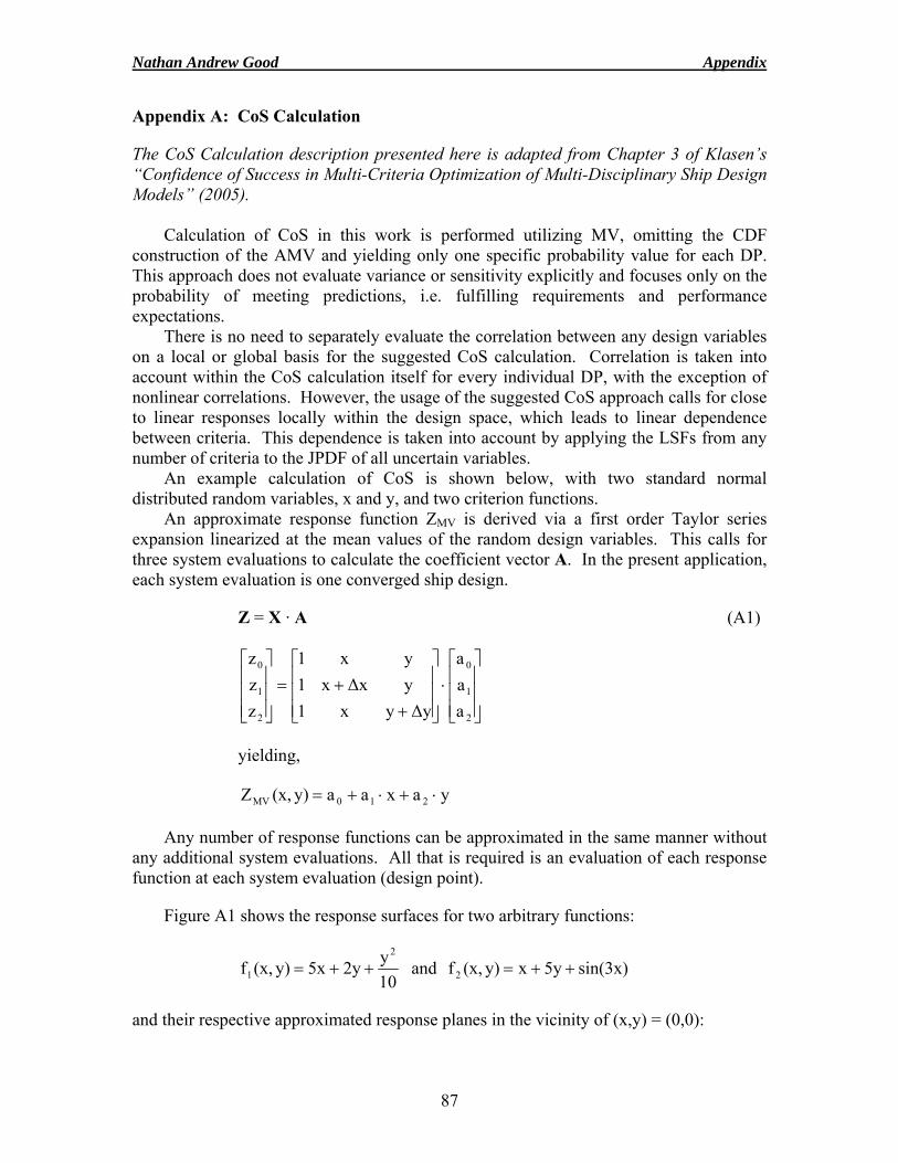
Nathan Andrew Good Appendix
87
Appendix A: CoS Calculation
The CoS Calculation description presented here is adapted from Chapter 3 of Klasen’s “Confidence of Success in Multi-Criteria Optimization of Multi-Disciplinary Ship Design Models” (2005).
Calculation of CoS in this work is performed utilizing MV, omitting the CDF
construction of the AMV and yielding only one specific probability value for each DP. This approach does not evaluate variance or sensitivity explicitly and focuses only on the probability of meeting predictions, i.e. fulfilling requirements and performance expectations.
There is no need to separately evaluate the correlation between any design variables on a local or global basis for the suggested CoS calculation. Correlation is taken into account within the CoS calculation itself for every individual DP, with the exception of nonlinear correlations. However, the usage of the suggested CoS approach calls for close to linear responses locally within the design space, which leads to linear dependence between criteria. This dependence is taken into account by applying the LSFs from any number of criteria to the JPDF of all uncertain variables.
An example calculation of CoS is shown below, with two standard normal distributed random variables, x and y, and two criterion functions.
An approximate response function ZMV is derived via a first order Taylor series expansion linearized at the mean values of the random design variables. This calls for three system evaluations to calculate the coefficient vector A. In the present application, each system evaluation is one converged ship design.
Z = X · A (A1)
⎥⎥⎥
⎦
⎤
⎢⎢⎢
⎣
⎡⋅
⎥⎥⎥
⎦
⎤
⎢⎢⎢
⎣
⎡
++=
⎥⎥⎥
⎦
⎤
⎢⎢⎢
⎣
⎡
2
1
0
2
1
0
aaa
Δyyx1yΔxx1yx1
zzz
yielding,
yaxaay)(x,Z 210MV ⋅+⋅+=
Any number of response functions can be approximated in the same manner without any additional system evaluations. All that is required is an evaluation of each response function at each system evaluation (design point).
Figure A1 shows the response surfaces for two arbitrary functions:
10y2y5xy)(x,f
2
1 ++= and sin(3x)5yxy)(x,f 2 ++=
and their respective approximated response planes in the vicinity of (x,y) = (0,0):
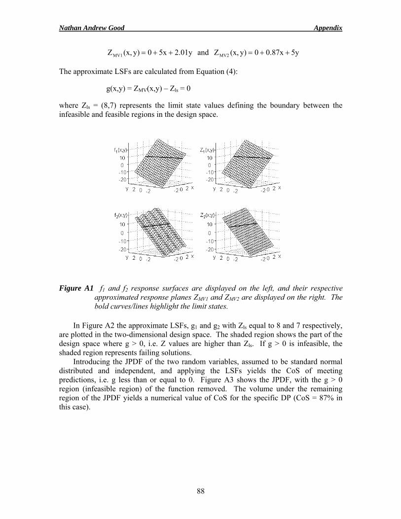
Nathan Andrew Good Appendix
88
2.01y5x0y)(x,ZMV1 ++= and 5y0.87x0y)(x,ZMV2 ++=
The approximate LSFs are calculated from Equation (4):
g(x,y) = ZMV(x,y) – Zls = 0
where Zls = (8,7) represents the limit state values defining the boundary between the infeasible and feasible regions in the design space.
In Figure A2 the approximate LSFs, g1 and g2 with Zls equal to 8 and 7 respectively, are plotted in the two-dimensional design space. The shaded region shows the part of the design space where g > 0, i.e. Z values are higher than Zls. If g > 0 is infeasible, the shaded region represents failing solutions.
Introducing the JPDF of the two random variables, assumed to be standard normal distributed and independent, and applying the LSFs yields the CoS of meeting predictions, i.e. g less than or equal to 0. Figure A3 shows the JPDF, with the g > 0 region (infeasible region) of the function removed. The volume under the remaining region of the JPDF yields a numerical value of CoS for the specific DP (CoS = 87% in this case).
Figure A1 f1 and f2 response surfaces are displayed on the left, and their respective approximated response planes ZMV1 and ZMV2 are displayed on the right. The bold curves/lines highlight the limit states.
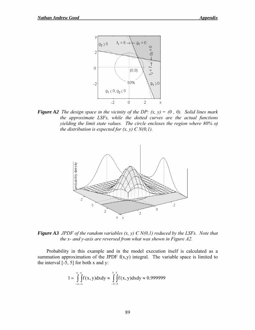
Nathan Andrew Good Appendix
89
Probability in this example and in the model execution itself is calculated as a summation approximation of the JPDF f(x,y) integral. The variable space is limited to the interval [-5, 5] for both x and y:
0.999999dxdy)y,x(fdxdy)y,x(f15
5
5
5
≈≈= ∫ ∫∫ ∫− −
∞
∞−
∞
∞−
Figure A3 JPDF of the random variables (x, y) Є N(0,1) reduced by the LSFs. Note that the x- and y-axis are reversed from what was shown in Figure A2.
Figure A2 The design space in the vicinity of the DP: (x, y) = (0 , 0). Solid lines mark the approximate LSFs, while the dotted curves are the actual functions yielding the limit state values. The circle encloses the region where 80% ofthe distribution is expected for (x, y) Є N(0,1).
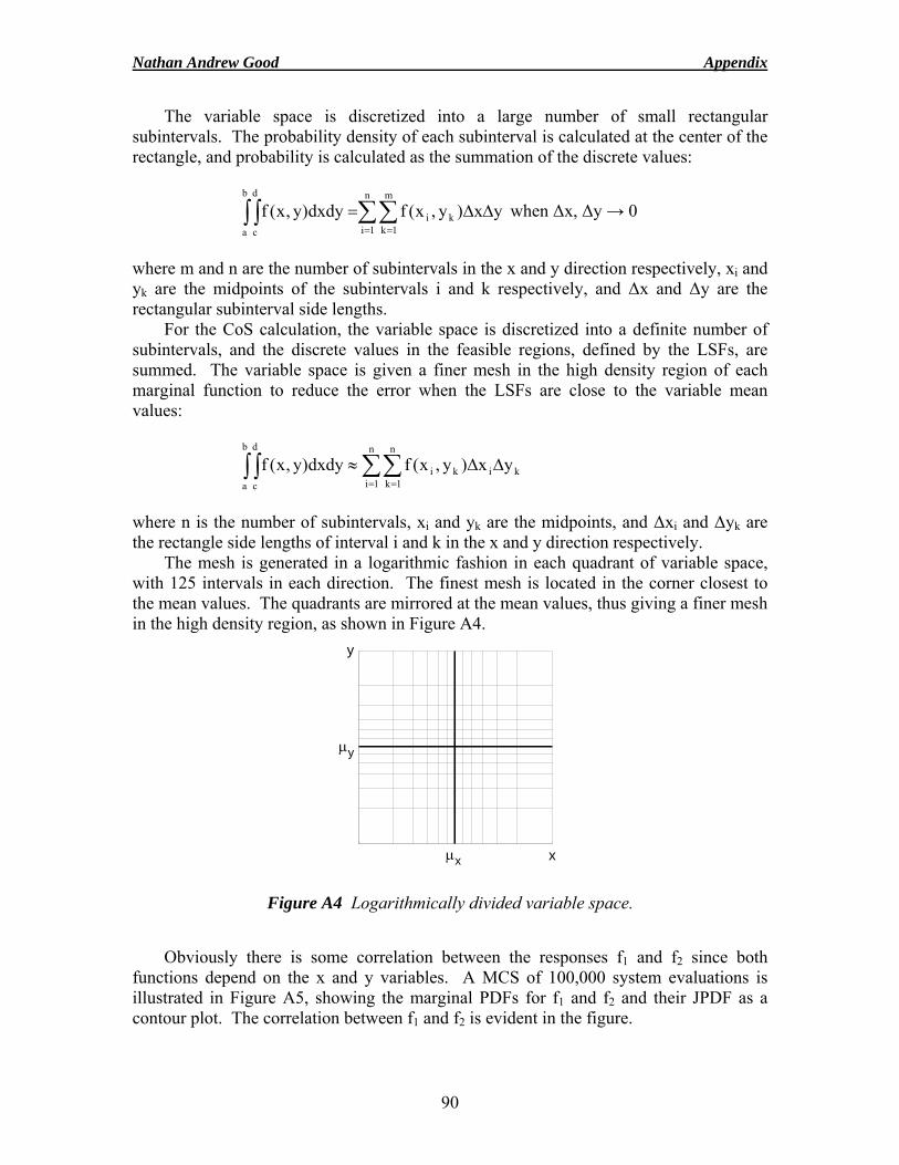
Nathan Andrew Good Appendix
90
The variable space is discretized into a large number of small rectangular subintervals. The probability density of each subinterval is calculated at the center of the rectangle, and probability is calculated as the summation of the discrete values:
∑∑∫ ∫= =
ΔΔ=n
1i
m
1kki
b
a
d
c
yx)y,x(fdxdy)y,x(f when Δx, Δy → 0
where m and n are the number of subintervals in the x and y direction respectively, xi and yk are the midpoints of the subintervals i and k respectively, and Δx and Δy are the rectangular subinterval side lengths.
For the CoS calculation, the variable space is discretized into a definite number of subintervals, and the discrete values in the feasible regions, defined by the LSFs, are summed. The variable space is given a finer mesh in the high density region of each marginal function to reduce the error when the LSFs are close to the variable mean values:
∑∑∫ ∫= =
ΔΔ≈n
1i
n
1kkiki
b
a
d
c
yx)y,x(fdxdy)y,x(f
where n is the number of subintervals, xi and yk are the midpoints, and Δxi and Δyk are the rectangle side lengths of interval i and k in the x and y direction respectively.
The mesh is generated in a logarithmic fashion in each quadrant of variable space, with 125 intervals in each direction. The finest mesh is located in the corner closest to the mean values. The quadrants are mirrored at the mean values, thus giving a finer mesh in the high density region, as shown in Figure A4.
x
y
μx
μy
Obviously there is some correlation between the responses f1 and f2 since both functions depend on the x and y variables. A MCS of 100,000 system evaluations is illustrated in Figure A5, showing the marginal PDFs for f1 and f2 and their JPDF as a contour plot. The correlation between f1 and f2 is evident in the figure.
Figure A4 Logarithmically divided variable space.
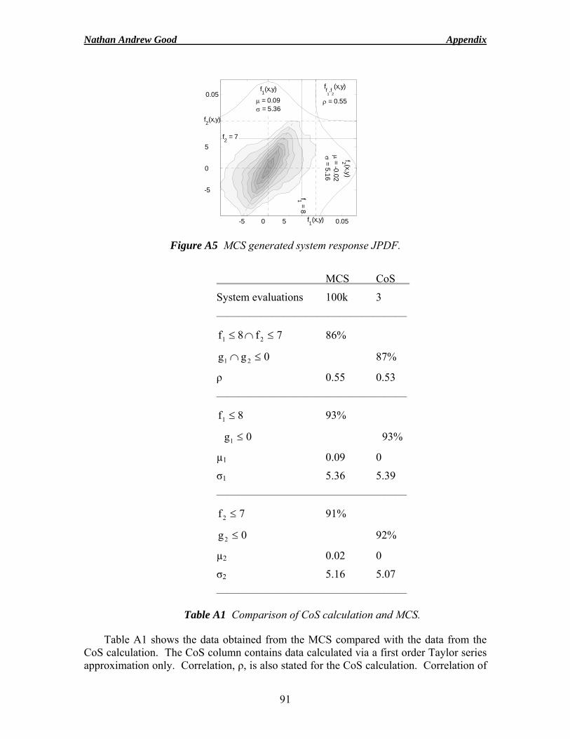
Nathan Andrew Good Appendix
91
f1(x,y)
μ = 0.09σ = 5.36
f2 (x,y)
μ = -0.02σ = 5.16
ff1,f
2
(x,y)
ρ = 0.55
f2 = 7
f1 = 8
f1(x,y)
f2(x,y)
-5 0 5 0.05
-5
0
5
0.05
Table A1 shows the data obtained from the MCS compared with the data from the
CoS calculation. The CoS column contains data calculated via a first order Taylor series approximation only. Correlation, ρ, is also stated for the CoS calculation. Correlation of
Figure A5 MCS generated system response JPDF.
MCS CoS
System evaluations 100k 3
—————————————————
7f8f 21 ≤∩≤ 86%
0gg 21 ≤∩ 87%
ρ 0.55 0.53
—————————————————
8f1 ≤ 93%
0g1 ≤ 93%
µ1 0.09 0
σ1 5.36 5.39
—————————————————
7f2 ≤ 91%
0g2 ≤ 92%
µ2 0.02 0
σ2 5.16 5.07
—————————————————
Table A1 Comparison of CoS calculation and MCS.
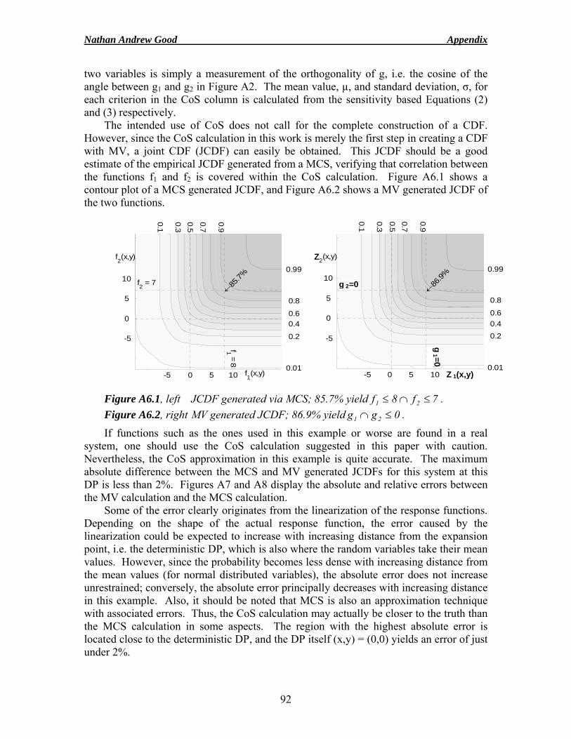
Nathan Andrew Good Appendix
92
two variables is simply a measurement of the orthogonality of g, i.e. the cosine of the angle between g1 and g2 in Figure A2. The mean value, µ, and standard deviation, σ, for each criterion in the CoS column is calculated from the sensitivity based Equations (2) and (3) respectively.
The intended use of CoS does not call for the complete construction of a CDF. However, since the CoS calculation in this work is merely the first step in creating a CDF with MV, a joint CDF (JCDF) can easily be obtained. This JCDF should be a good estimate of the empirical JCDF generated from a MCS, verifying that correlation between the functions f1 and f2 is covered within the CoS calculation. Figure A6.1 shows a contour plot of a MCS generated JCDF, and Figure A6.2 shows a MV generated JCDF of the two functions.
If functions such as the ones used in this example or worse are found in a real
system, one should use the CoS calculation suggested in this paper with caution. Nevertheless, the CoS approximation in this example is quite accurate. The maximum absolute difference between the MCS and MV generated JCDFs for this system at this DP is less than 2%. Figures A7 and A8 display the absolute and relative errors between the MV calculation and the MCS calculation.
Some of the error clearly originates from the linearization of the response functions. Depending on the shape of the actual response function, the error caused by the linearization could be expected to increase with increasing distance from the expansion point, i.e. the deterministic DP, which is also where the random variables take their mean values. However, since the probability becomes less dense with increasing distance from the mean values (for normal distributed variables), the absolute error does not increase unrestrained; conversely, the absolute error principally decreases with increasing distance in this example. Also, it should be noted that MCS is also an approximation technique with associated errors. Thus, the CoS calculation may actually be closer to the truth than the MCS calculation in some aspects. The region with the highest absolute error is located close to the deterministic DP, and the DP itself (x,y) = (0,0) yields an error of just under 2%.
Figure A6.1, left JCDF generated via MCS; 85.7% yield 7f8f 21 ≤∩≤ . Figure A6.2, right MV generated JCDF; 86.9% yield 0gg 21 ≤∩ .
0.99
0.9
0.8
0.7
0.6
0.5
0.4
0.3
0.2
0.1
0.01
←85
.7% f2 = 7
f1 = 8
f1(x,y)
f2(x,y)
-5 0 5 10
-5
0
5
10
0.99
0.9
0.8
0.7
0.6
0.5
0.4
0.3
0.2
0.1
0.01
←86
.9% f2 = 7
f1 = 8
f1(x,y)
f2(x,y)
-5 0 5 10
-5
0
5
10
Z
g 2=0
g 1 =0
Z 1(x,y)
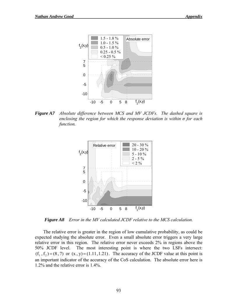
Nathan Andrew Good Appendix
93
Absolute error
f1(x,y)
f2(x,y)
-10 -5 0 5 8
-10
-5
0
5 7
1.5 - 1.8 %1.0 - 1.5 %0.5 - 1.0 %0.25 - 0.5 %< 0.25 %
Relative error
f1(x,y)
f2(x,y)
-10 -5 0 5 8
-10
-5
0
5 7
20 - 30 %10 - 20 %5 - 10 %2 - 5 %< 2 %
The relative error is greater in the region of low cumulative probability, as could be expected studying the absolute error. Even a small absolute error triggers a very large relative error in this region. The relative error never exceeds 2% in regions above the 50% JCDF level. The most interesting point is where the two LSFs intersect:
7) , (8 )f , (f 21 = or 1.21) , (1.11 y) ,(x = . The accuracy of the JCDF value at this point is an important indicator of the accuracy of the CoS calculation. The absolute error here is 1.2% and the relative error is 1.4%.
Figure A8 Error in the MV calculated JCDF relative to the MCS calculation.
Figure A7 Absolute difference between MCS and MV JCDFs. The dashed square is enclosing the region for which the response deviation is within σ for each function.
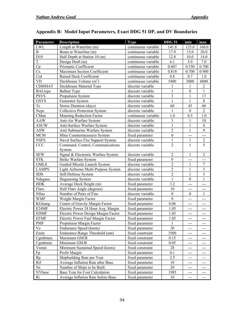
Nathan Andrew Good Appendix
94
Appendix B: Model Input Parameters, Exact DDG 51 DP, and DV Boundaries
Parameter Description Type DDG 51 min max LWL Length at Waterline (m) continuous variable 141.8 125.0 160.0B Beam at Waterline (m) continuous variable 17.9 15.0 20.0 D10 Hull Depth at Station 10 (m) continuous variable 12.8 10.0 14.0 T Design Draft (m) continuous variable 6.1 5.0 7.0 Cp Prismatic Coefficient continuous variable 0.607 0.550 0.700Cx Maximum Section Coefficient continuous variable 0.818 0.700 0.900Crd Raised Deck Coefficient continuous variable 0.8 0.7 1.0 VD Deckhouse Volume (m3) continuous variable 5400 3000 6000 CDHMAT Deckhouse Material Type discrete variable 1 1 2 BALtype Ballast Type discrete variable 1 0 1 PSYS Propulsion System discrete variable 3 1 17 GSYS Generator System discrete variable 1 1 8 Ts Stores Duration (days) discrete variable 60 45 60 Ncps Collective Protection System discrete variable 1 0 2 CMan Manning Reduction Factor continuous variable 1.0 0.5 1.0 AAW Anti-Air Warfare System discrete variable 3 1 10 ASUW Anti-Surface Warfare System discrete variable 1 1 4 ASW Anti-Submarine Warfare System discrete variable 2 1 9 MCM Mine Countermeasures System fixed parameter 0 --- --- NSFS Naval Surface Fire Support System discrete variable 1 1 2 CCC Command, Control, Communications
System discrete variable 2 1 5
SEW Signal & Electronic Warfare System discrete variable 2 1 2 STK Strike Warfare System fixed parameter 0 --- --- GMLS Guided Missile Launch System discrete variable 2 1 7 LAMPS Light Airborne Multi-Purpose System discrete variable 2 1 3 SDS Self-Defense System discrete variable 2 1 3 Ndegaus Degaussing System discrete variable 1 0 1 HDK Average Deck Height (m) fixed parameter 3.2 --- --- Flare Hull Flare Angle (degrees) fixed parameter 10 --- --- Nfins Number of Pairs of Fins discrete variable 0 0 1 WMF Weight Margin Factor fixed parameter 0 --- --- KGmarg Center of Gravity Margin Factor fixed parameter 0.06 --- --- E24MF Electric Power 24 Hour Avg. Margin fixed parameter 1.05 --- --- EDMF Electric Power Design Margin Factor fixed parameter 1.05 --- --- EFMF Electric Power Fuel Margin Factor fixed parameter 1.05 --- --- PMF Propulsion Margin Factor fixed parameter 1 --- --- Ve Endurance Speed (knots) fixed parameter 20 --- --- Emin Endurance Range Threshold (nm) fixed constraint 3500 --- --- Cgmbmax Maximum GM/B fixed constraint 0.15 --- --- Cgmbmin Minimum GM/B fixed constraint 0.05 --- --- Vsmin Minimum Sustained Speed (knots) fixed constraint 28 --- --- Fp Profit Margin fixed parameter 0.1 --- --- Rp Shipbuilding Rate per Year fixed parameter 2.5 --- --- Rif Average Inflation Rate after Base fixed parameter 10 --- --- Ns Number of Ships to be Built fixed parameter 20 --- --- NYbase Base Year for Cost Calculation fixed parameter 1985 --- --- Ri Average Inflation Rate before Base fixed parameter 10 --- ---
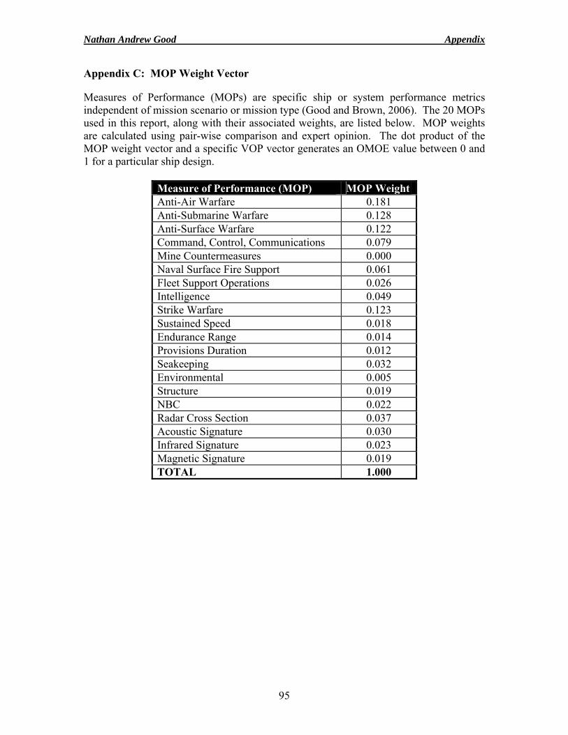
Nathan Andrew Good Appendix
95
Appendix C: MOP Weight Vector
Measures of Performance (MOPs) are specific ship or system performance metrics independent of mission scenario or mission type (Good and Brown, 2006). The 20 MOPs used in this report, along with their associated weights, are listed below. MOP weights are calculated using pair-wise comparison and expert opinion. The dot product of the MOP weight vector and a specific VOP vector generates an OMOE value between 0 and 1 for a particular ship design.
Measure of Performance (MOP) MOP Weight Anti-Air Warfare 0.181 Anti-Submarine Warfare 0.128 Anti-Surface Warfare 0.122 Command, Control, Communications 0.079 Mine Countermeasures 0.000 Naval Surface Fire Support 0.061 Fleet Support Operations 0.026 Intelligence 0.049 Strike Warfare 0.123 Sustained Speed 0.018 Endurance Range 0.014 Provisions Duration 0.012 Seakeeping 0.032 Environmental 0.005 Structure 0.019 NBC 0.022 Radar Cross Section 0.037 Acoustic Signature 0.030 Infrared Signature 0.023 Magnetic Signature 0.019 TOTAL 1.000
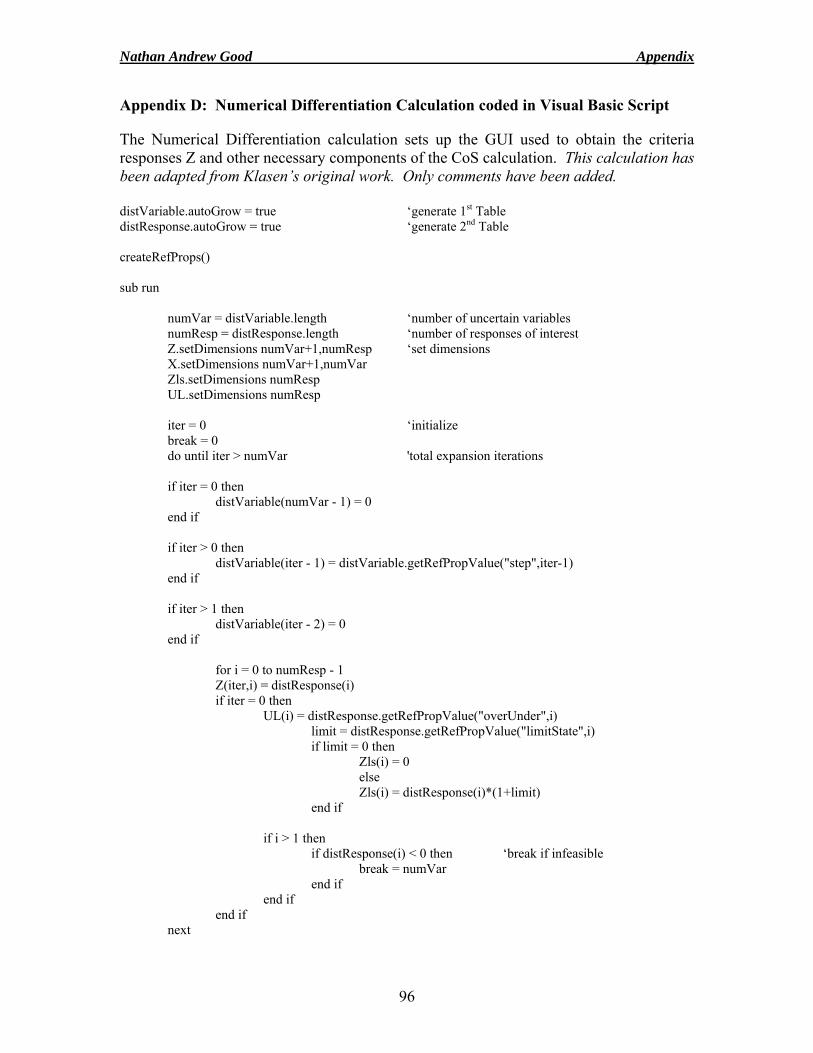
Nathan Andrew Good Appendix
96
Appendix D: Numerical Differentiation Calculation coded in Visual Basic Script
The Numerical Differentiation calculation sets up the GUI used to obtain the criteria responses Z and other necessary components of the CoS calculation. This calculation has been adapted from Klasen’s original work. Only comments have been added. distVariable.autoGrow = true ‘generate 1st Table distResponse.autoGrow = true ‘generate 2nd Table createRefProps() sub run numVar = distVariable.length ‘number of uncertain variables numResp = distResponse.length ‘number of responses of interest Z.setDimensions numVar+1,numResp ‘set dimensions X.setDimensions numVar+1,numVar Zls.setDimensions numResp UL.setDimensions numResp iter = 0 ‘initialize break = 0 do until iter > numVar 'total expansion iterations if iter = 0 then distVariable(numVar - 1) = 0 end if if iter > 0 then distVariable(iter - 1) = distVariable.getRefPropValue("step",iter-1) end if if iter > 1 then distVariable(iter - 2) = 0 end if for i = 0 to numResp - 1 Z(iter,i) = distResponse(i) if iter = 0 then UL(i) = distResponse.getRefPropValue("overUnder",i) limit = distResponse.getRefPropValue("limitState",i) if limit = 0 then Zls(i) = 0 else Zls(i) = distResponse(i)*(1+limit) end if if i > 1 then if distResponse(i) < 0 then ‘break if infeasible break = numVar end if end if end if next
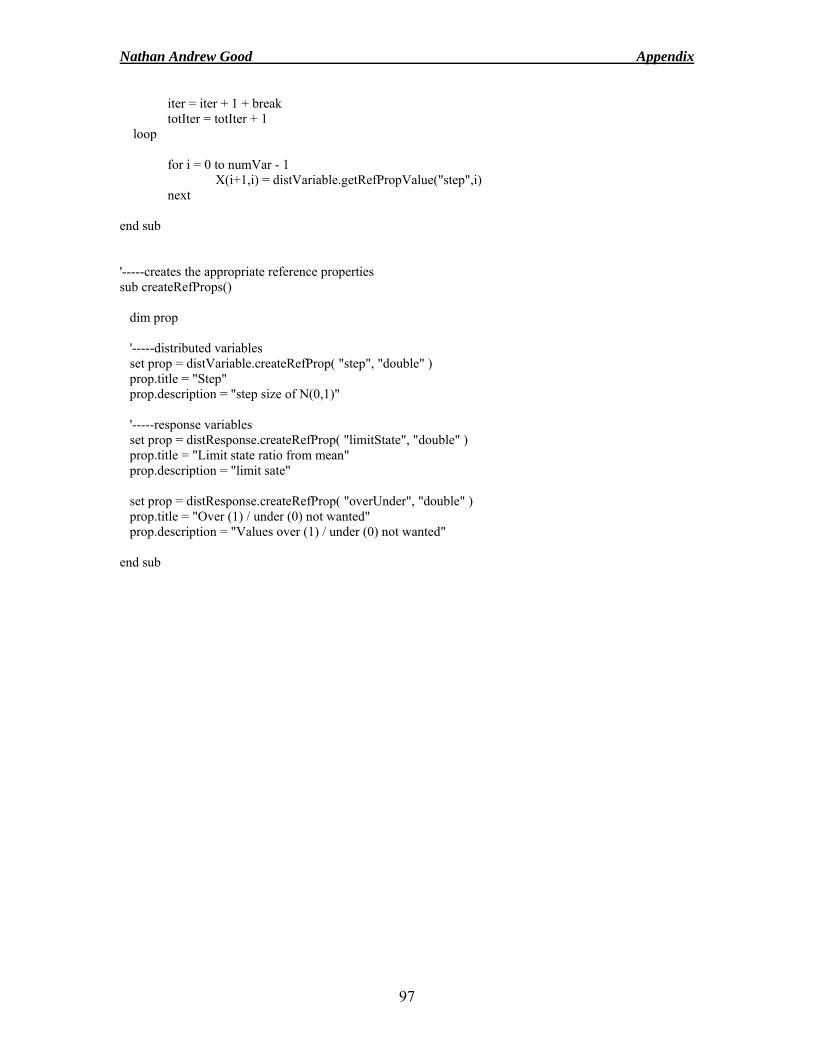
Nathan Andrew Good Appendix
97
iter = iter + 1 + break totIter = totIter + 1 loop for i = 0 to numVar - 1 X(i+1,i) = distVariable.getRefPropValue("step",i) next end sub '-----creates the appropriate reference properties sub createRefProps() dim prop '-----distributed variables set prop = distVariable.createRefProp( "step", "double" ) prop.title = "Step" prop.description = "step size of N(0,1)" '-----response variables set prop = distResponse.createRefProp( "limitState", "double" ) prop.title = "Limit state ratio from mean" prop.description = "limit sate" set prop = distResponse.createRefProp( "overUnder", "double" ) prop.title = "Over (1) / under (0) not wanted" prop.description = "Values over (1) / under (0) not wanted" end sub
Nathan Andrew Good Appendix
98
Appendix E: 2 Variable CoS Calculation coded in Matlab
This Confidence of Success (CoS) calculation determines the CoS value of a particular DP as well as each individual criterion’s probability of feasibility. It is only functional for two standard normal distributed uncertain variables. This calculation has been adapted from Klasen’s original work. Only comments have been added. % CoS - only functional for two standard normal distributed variables % Zls - limit state value % UL - 1 for cutaway of values > Zls and 0 for cutaway of values < Zls respnum = length(Z(1,:)); % number of responses of interest varnum = length(Z(:,1)) - 1; % number of standard normal distributed variables, must be two! X = [ones(max(size(X)),1) X]; % variable expansion values span = 5; % sets outer boundaries for standard normal distributed variables respjpdf=[]; % sets empty placeholders meanZ = Z(1,:)'; % transpose of meanZ vector if any(Z(1,3:respnum)<0) % if infeasible, CoS = 0 CoS = 0; respPoF = zeros(respnum,1); Z(2:varnum+1,:) = 0; A = zeros(varnum+1,respnum); else for i = 1:respnum A(:,i) = X \ Z(:,i); % produces A vector for every response end t=logspace(0,log(span+1)/log(10),ceil(span*25))-1; tint = [t 0]-[0 t]; t=[0 t] + tint/2; t=t(2:length(t)-1); tint=tint(2:length(tint)-1); ttemp = [-rot90(t); t']; % generates logarithmically spaced vector for i = 1:respnum [Yz,Xz,LS] = ndgrid(A(3,i)*ttemp,A(2,i)*ttemp,A(1,i)-Zls(i)); % ndgrid generates arrays for multidimensional functions and interpolation check = Xz + Yz + LS; % creates a limit state value for all coordinates if UL(i) == 1 % UL - 1 for cutaway of values > Zls and 0 for cutaway of values < Zls area = (check + abs(check)); % creates zeros where it's supposed to be ones – sets all feasible (negative) values equal to zero else area = (check - abs(check)); % creates zeros where it's supposed to be ones – sets all feasible (positive) values equal to zero end warning off %MATLAB:divideByZero; respjpdf(:,:,i) = isnan(area ./ area); % creates ones in place of NaN, caused by division with zero; all real numbers are set equal to zero warning on %MATLAB:divideByZero end
Nathan Andrew Good Appendix
99
domain = prod(respjpdf,3); % determines coordinates that are feasible for all responses; feasible coordinates are assigned a value of 1, infeasible coordinates a value of zero. jpdf = (normpdf(t)' * normpdf(t)) .* (tint' * tint); % generates quadrant I of jpdf jpdf = [fliplr(jpdf) jpdf]; % mirrors jpdf over y-axis jpdf = [flipud(jpdf); jpdf]; % mirrors jpdf over x-axis CoS = sum(sum(domain .* jpdf)); % summation of each domain point multiplied by its corresponding jpdf value respPoF = squeeze(sum(sum(respjpdf .* repmat(jpdf,[1 1 respnum])))); % probability of feasibility for each particular response. end % output to Excel file fid = fopen(filename,'a'); fprintf(fid,'%12.8f\t',clock); fprintf(fid,'%12.8f\t',CoS); fprintf(fid,'%12.8f\t',meanZ); fprintf(fid,'%12.8f\t',respPoF); fprintf(fid,'%12.8f\t',Z); fprintf(fid,'%12.8f\t',A); fprintf(fid,'%12.8f\t',RT); fprintf(fid,'%12.8f\t',Wls); fprintf(fid,'%12.8f\t',designvariables); fprintf(fid,'\n'); fclose(fid);
Nathan Andrew Good Appendix
100
Appendix F: 3 Variable CoS Calculation coded in Matlab
This Confidence of Success (CoS) calculation is only functional for three standard normal distributed uncertain variables. % CoS - functional for three standard normal distributed variables % Zls - limit state value % UL - 1 for cutaway of values > Zls and 0 for cutaway of values < Zls respnum=length(Z(1,:)); % number of responses of interest varnum=length(Z(:,1))-1; % number of standard normal distributed variables X=[ones(max(size(X)),1) X]; % variable expansion values span=3; % sets outer boundaries for standard normal distributed variables respjpdf=[]; % sets empty placeholders check=[]; jpdf=[]; A=zeros(varnum+1,respnum); meanZ=Z(1,:)'; % transpose of meanZ vector X1=[]; % sets empty placeholders X2=[]; X3=[]; LS=[]; if any(Z(1,3:respnum)<0) % if infeasible, CoS = 0 CoS=0; respPoF=zeros(respnum,1); Z(2:varnum+1,:)=0; A=zeros(varnum+1,respnum); else for i=1:respnum A(:,i)=X\Z(:,i); % produces A vector for every response end spacing=10; % number of subdivisions per unit span t=logspace(0,log(span+1)/log(10),ceil(span*spacing))-1; tint=[t 0]-[0 t]; t=[0 t]+tint/2; t=t(2:length(t)-1); tint=tint(2:length(tint)-1); ttemp=[-rot90(t);t']; % generates logarithmically spaced vector for i=1:respnum [X3,X2,X1,LS]=ndgrid(A(4,i)*ttemp,A(3,i)*ttemp,A(2,i)*ttemp,A(1,i)-Zls(i)); % ndgrid generates arrays for multidimensional functions and interpolation check=LS+X1+X2+X3; % creates a limit state value for all coordinates if UL(i)==1 % UL - 1 for cutaway of values > Zls and 0 for cutaway of values < Zls area=(check+abs(check)); % creates zeros where it's supposed to be ones - sets all feasible (negative) values equal to zero else area=(check-abs(check)); % creates zeros where it's supposed to be ones - sets all feasible (positive) values equal to zero end warning off %MATLAB:divideByZero respjpdf(:,:,:,i)=isnan(area./area); % creates ones in place of NaN, caused by division with zero - all real numbers are set equal to zero warning on %MATLAB:divideByZero
Nathan Andrew Good Appendix
101
end clear X Zls UL varnum check t limitstate X1 X2 X3 area % clears parameters no longer needed domain=prod(respjpdf,4); % determines coordinates that are feasible for all responses - feasible coordinates are assigned a value of 1, infeasible coordinates a value of zero. tint=[fliplr(tint) tint]; % t interval vector Norm=normpdf(ttemp); % Norm pdf vector for j=1:(2*spacing*span-2) for k=1:(2*spacing*span-2) for m=1:(2*spacing*span-2) jpdf(j,k,m)=(Norm(j)*Norm(k)*Norm(m)).*(tint(j)*tint(k)*tint(m)); % produces 3-D jpdf end end end CoS=sum(sum(sum(domain.*jpdf))); % summation of each domain point multiplied by its corresponding jpdf value clear domain % clear parameter domain respPoF=squeeze(sum(sum(sum(respjpdf.*repmat(jpdf,[1 1 1 respnum]))))); % probability of feasibility for each particular response. end % output to Excel file fid = fopen(filename,'a'); fprintf(fid,'%12.8f\t',clock); fprintf(fid,'%12.8f\t',CoS); fprintf(fid,'%12.8f\t',meanZ); fprintf(fid,'%12.8f\t',respPoF); fprintf(fid,'%12.8f\t',Z); fprintf(fid,'%12.8f\t',A); fprintf(fid,'%12.8f\t',RT); fprintf(fid,'%12.8f\t',Wlso); fprintf(fid,'%12.8f\t',KGo); fprintf(fid,'%12.8f\t',designvariables); fprintf(fid,'\n'); fclose(fid);
Nathan Andrew Good Appendix
102
Appendix G: 4 Variable CoS Calculation coded in Matlab
This Confidence of Success (CoS) calculation is only functional for four standard normal distributed uncertain variables. % CoS - functional for four standard normal distributed variables % Zls - limit state value % UL - 1 for cutaway of values > Zls and 0 for cutaway of values < Zls respnum=length(Z(1,:)); % number of responses of interest varnum=length(Z(:,1))-1; % number of standard normal distributed variables X=[ones(max(size(X)),1) X]; % variable expansion values span=3; % sets outer boundaries for standard normal distributed variables respjpdf=[]; % sets empty placeholders check=[]; jpdf=[]; A=zeros(varnum+1,respnum); meanZ=Z(1,:)'; % transpose of meanZ vector X1=[]; % sets empty placeholders X2=[]; X3=[]; X4=[]; LS=[]; if any(Z(1,3:respnum)<0) % if infeasible, CoS = 0 CoS=0; respPoF=zeros(respnum,1); Z(2:varnum+1,:)=0; A=zeros(varnum+1,respnum); else for i=1:respnum A(:,i)=X\Z(:,i); % produces A vector for every response end spacing=4; % number of subdivisions per unit span t=logspace(0,log(span+1)/log(10),ceil(span*spacing))-1; tint=[t 0]-[0 t]; t=[0 t]+tint/2; t=t(2:length(t)-1); tint=tint(2:length(tint)-1); ttemp=[-rot90(t);t']; % generates logarithmically spaced vector for i=1:respnum [X4,X3,X2,X1,LS]=ndgrid(A(5,i)*ttemp,A(4,i)*ttemp,A(3,i)*ttemp,A(2,i)*ttemp,A(1,i)-Zls(i)); % ndgrid generates arrays for multidimensional functions and interpolation check=LS+X1+X2+X3+X4; % creates a limit state value for all coordinates if UL(i)==1 % UL - 1 for cutaway of values > Zls and 0 for cutaway of values < Zls area=(check+abs(check)); % creates zeros where it's supposed to be ones - sets all feasible (negative) values equal to zero else area=(check-abs(check)); % creates zeros where it's supposed to be ones - sets all feasible (positive) values equal to zero end warning off %MATLAB:divideByZero respjpdf(:,:,:,:,i)=isnan(area./area); % creates ones in place of NaN, caused by division with zero - all real numbers are set equal to zero
Nathan Andrew Good Appendix
103
warning on %MATLAB:divideByZero end clear X Zls UL varnum check t limitstate X1 X2 X3 X4 area % clears parameters no longer needed domain=prod(respjpdf,5); % determines coordinates that are feasible for all responses - feasible coordinates are assigned a value of 1, infeasible coordinates a value of zero. tint=[fliplr(tint) tint]; % t interval vector Norm=normpdf(ttemp); % Norm pdf vector for j=1:(2*spacing*span-2) for k=1:(2*spacing*span-2) for m=1:(2*spacing*span-2) for n=1:(2*spacing*span-2) jpdf(j,k,m,n)=(Norm(j)*Norm(k)*Norm(m)*Norm(n)).*(tint(j)*tint(k)*tint(m)*tint(n)); % produces 4-D jpdf end end end end CoS=sum(sum(sum(sum(domain.*jpdf)))); % summation of each domain point multiplied by its corresponding jpdf value clear domain % clear parameter domain respPoF=squeeze(sum(sum(sum(sum(respjpdf.*repmat(jpdf,[1 1 1 1 respnum])))))); % probability of feasibility for each particular response. end % output to Excel file fid = fopen(filename,'a'); fprintf(fid,'%12.8f\t',clock); fprintf(fid,'%12.8f\t',CoS); fprintf(fid,'%12.8f\t',meanZ); fprintf(fid,'%12.8f\t',respPoF); fprintf(fid,'%12.8f\t',Z); fprintf(fid,'%12.8f\t',A); fprintf(fid,'%12.8f\t',RT); fprintf(fid,'%12.8f\t',W16); fprintf(fid,'%12.8f\t',W235); fprintf(fid,'%12.8f\t',W47); fprintf(fid,'%12.8f\t',designvariables); fprintf(fid,'\n'); fclose(fid);
Nathan Andrew Good Appendix
104
Appendix H: Penalty Function coded in Matlab
This penalty function penalizes designs in the proximity of others to encourage a more uniform distribution of points across the Pareto front. Its concept is described in detail in Section 5.4. % Penalty Function % design - overall design number % population - population size % constraint - acceptable distance squared value % penalty - % penalty applied generation=floor((design-1)/population)+1; % generation number check=(design-1)/population+1; % new generation check popnum=(check-generation)*population+1; % design # in current population if generation==check % new generation CTOCv=[]; % initialize objective vectors OMOEv=[]; CoSv=[]; CTOCv(1)=CTOC; % first entry of new generation objective vectors OMOEv(1)=OMOE; CoSv(1)=CoS; CTOCnew=CTOC; % no penalties applied OMOEnew=OMOE; CoSnew=CoS; else CTOCv(popnum)=CTOC; % add entry to objective vectors OMOEv(popnum)=OMOE; CoSv(popnum)=CoS; distsq=[]; % initialize distsq vector CTOCnew=CTOC; OMOEnew=OMOE; CoSnew=CoS; for i=1:(popnum-1) distsq(i)=((CTOCv(popnum)-CTOCv(i))/1000)^2+(OMOEv(popnum)-OMOEv(i))^2+(CoSv(popnum)-CoSv(i))^2; % calculates distance squared between current DP and all previous DPs if distsq(i) <= constraint % constraint violation CTOCnew=(1+penalty)*CTOCnew; % penalties applied OMOEnew=(1-penalty)*OMOEnew; CoSnew=(1-penalty)*CoSnew; Else % no violation CTOCnew=CTOCnew; % no penalties applied OMOEnew=OMOEnew; CoSnew=CoSnew; end end end % output to Excel file fid = fopen(filename2,'a'); fprintf(fid,'%12.8f\t',generation); fprintf(fid,'%12.8f\t',check);

Nathan Andrew Good Appendix
105
fprintf(fid,'%12.8f\t',popnum); fprintf(fid,'%12.8f\t',CTOCv); fprintf(fid,'%12.8f\t',OMOEv); fprintf(fid,'%12.8f\t',CoSv); fprintf(fid,'%12.8f\t',CTOCnew); fprintf(fid,'%12.8f\t',OMOEnew); fprintf(fid,'%12.8f\t',CoSnew); fprintf(fid,'%12.8f\t',distsq); fprintf(fid,'\n'); fclose(fid);
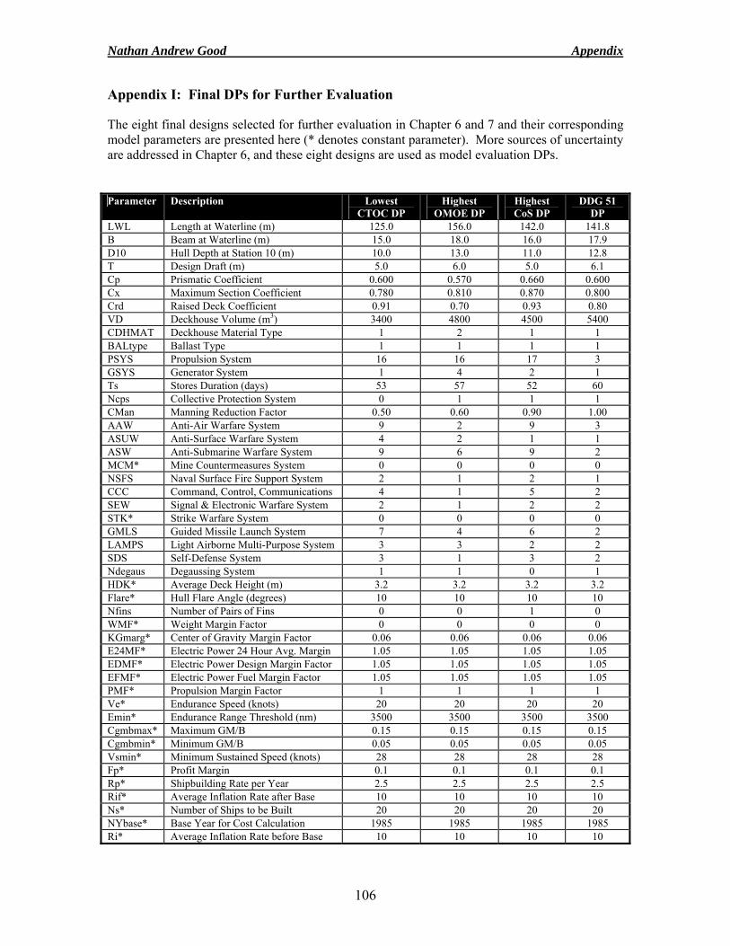
Nathan Andrew Good Appendix
106
Appendix I: Final DPs for Further Evaluation
The eight final designs selected for further evaluation in Chapter 6 and 7 and their corresponding model parameters are presented here (* denotes constant parameter). More sources of uncertainty are addressed in Chapter 6, and these eight designs are used as model evaluation DPs.
Parameter Description Lowest CTOC DP
Highest OMOE DP
Highest CoS DP
DDG 51 DP
LWL Length at Waterline (m) 125.0 156.0 142.0 141.8 B Beam at Waterline (m) 15.0 18.0 16.0 17.9 D10 Hull Depth at Station 10 (m) 10.0 13.0 11.0 12.8 T Design Draft (m) 5.0 6.0 5.0 6.1 Cp Prismatic Coefficient 0.600 0.570 0.660 0.600 Cx Maximum Section Coefficient 0.780 0.810 0.870 0.800 Crd Raised Deck Coefficient 0.91 0.70 0.93 0.80 VD Deckhouse Volume (m3) 3400 4800 4500 5400 CDHMAT Deckhouse Material Type 1 2 1 1 BALtype Ballast Type 1 1 1 1 PSYS Propulsion System 16 16 17 3 GSYS Generator System 1 4 2 1 Ts Stores Duration (days) 53 57 52 60 Ncps Collective Protection System 0 1 1 1 CMan Manning Reduction Factor 0.50 0.60 0.90 1.00 AAW Anti-Air Warfare System 9 2 9 3 ASUW Anti-Surface Warfare System 4 2 1 1 ASW Anti-Submarine Warfare System 9 6 9 2 MCM* Mine Countermeasures System 0 0 0 0 NSFS Naval Surface Fire Support System 2 1 2 1 CCC Command, Control, Communications 4 1 5 2 SEW Signal & Electronic Warfare System 2 1 2 2 STK* Strike Warfare System 0 0 0 0 GMLS Guided Missile Launch System 7 4 6 2 LAMPS Light Airborne Multi-Purpose System 3 3 2 2 SDS Self-Defense System 3 1 3 2 Ndegaus Degaussing System 1 1 0 1 HDK* Average Deck Height (m) 3.2 3.2 3.2 3.2 Flare* Hull Flare Angle (degrees) 10 10 10 10 Nfins Number of Pairs of Fins 0 0 1 0 WMF* Weight Margin Factor 0 0 0 0 KGmarg* Center of Gravity Margin Factor 0.06 0.06 0.06 0.06 E24MF* Electric Power 24 Hour Avg. Margin 1.05 1.05 1.05 1.05 EDMF* Electric Power Design Margin Factor 1.05 1.05 1.05 1.05 EFMF* Electric Power Fuel Margin Factor 1.05 1.05 1.05 1.05 PMF* Propulsion Margin Factor 1 1 1 1 Ve* Endurance Speed (knots) 20 20 20 20 Emin* Endurance Range Threshold (nm) 3500 3500 3500 3500 Cgmbmax* Maximum GM/B 0.15 0.15 0.15 0.15 Cgmbmin* Minimum GM/B 0.05 0.05 0.05 0.05 Vsmin* Minimum Sustained Speed (knots) 28 28 28 28 Fp* Profit Margin 0.1 0.1 0.1 0.1 Rp* Shipbuilding Rate per Year 2.5 2.5 2.5 2.5 Rif* Average Inflation Rate after Base 10 10 10 10 Ns* Number of Ships to be Built 20 20 20 20 NYbase* Base Year for Cost Calculation 1985 1985 1985 1985 Ri* Average Inflation Rate before Base 10 10 10 10
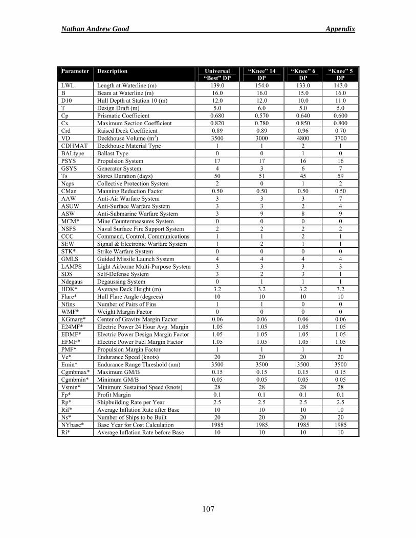
Nathan Andrew Good Appendix
107
Parameter Description Universal “Best” DP
“Knee” 14 DP
“Knee” 6 DP
“Knee” 5 DP
LWL Length at Waterline (m) 139.0 154.0 133.0 143.0 B Beam at Waterline (m) 16.0 16.0 15.0 16.0 D10 Hull Depth at Station 10 (m) 12.0 12.0 10.0 11.0 T Design Draft (m) 5.0 6.0 5.0 5.0 Cp Prismatic Coefficient 0.680 0.570 0.640 0.600 Cx Maximum Section Coefficient 0.820 0.780 0.850 0.800 Crd Raised Deck Coefficient 0.89 0.89 0.96 0.70 VD Deckhouse Volume (m3) 3500 3000 4800 3700 CDHMAT Deckhouse Material Type 1 1 2 1 BALtype Ballast Type 0 0 1 0 PSYS Propulsion System 17 17 16 16 GSYS Generator System 4 3 6 7 Ts Stores Duration (days) 50 51 45 59 Ncps Collective Protection System 2 0 1 2 CMan Manning Reduction Factor 0.50 0.50 0.50 0.50 AAW Anti-Air Warfare System 3 3 3 7 ASUW Anti-Surface Warfare System 3 3 2 4 ASW Anti-Submarine Warfare System 3 9 8 9 MCM* Mine Countermeasures System 0 0 0 0 NSFS Naval Surface Fire Support System 2 2 2 2 CCC Command, Control, Communications 1 1 2 1 SEW Signal & Electronic Warfare System 1 2 1 1 STK* Strike Warfare System 0 0 0 0 GMLS Guided Missile Launch System 4 4 4 4 LAMPS Light Airborne Multi-Purpose System 3 3 3 3 SDS Self-Defense System 3 2 3 1 Ndegaus Degaussing System 0 1 1 1 HDK* Average Deck Height (m) 3.2 3.2 3.2 3.2 Flare* Hull Flare Angle (degrees) 10 10 10 10 Nfins Number of Pairs of Fins 1 1 0 0 WMF* Weight Margin Factor 0 0 0 0 KGmarg* Center of Gravity Margin Factor 0.06 0.06 0.06 0.06 E24MF* Electric Power 24 Hour Avg. Margin 1.05 1.05 1.05 1.05 EDMF* Electric Power Design Margin Factor 1.05 1.05 1.05 1.05 EFMF* Electric Power Fuel Margin Factor 1.05 1.05 1.05 1.05 PMF* Propulsion Margin Factor 1 1 1 1 Ve* Endurance Speed (knots) 20 20 20 20 Emin* Endurance Range Threshold (nm) 3500 3500 3500 3500 Cgmbmax* Maximum GM/B 0.15 0.15 0.15 0.15 Cgmbmin* Minimum GM/B 0.05 0.05 0.05 0.05 Vsmin* Minimum Sustained Speed (knots) 28 28 28 28 Fp* Profit Margin 0.1 0.1 0.1 0.1 Rp* Shipbuilding Rate per Year 2.5 2.5 2.5 2.5 Rif* Average Inflation Rate after Base 10 10 10 10 Ns* Number of Ships to be Built 20 20 20 20 NYbase* Base Year for Cost Calculation 1985 1985 1985 1985 Ri* Average Inflation Rate before Base 10 10 10 10
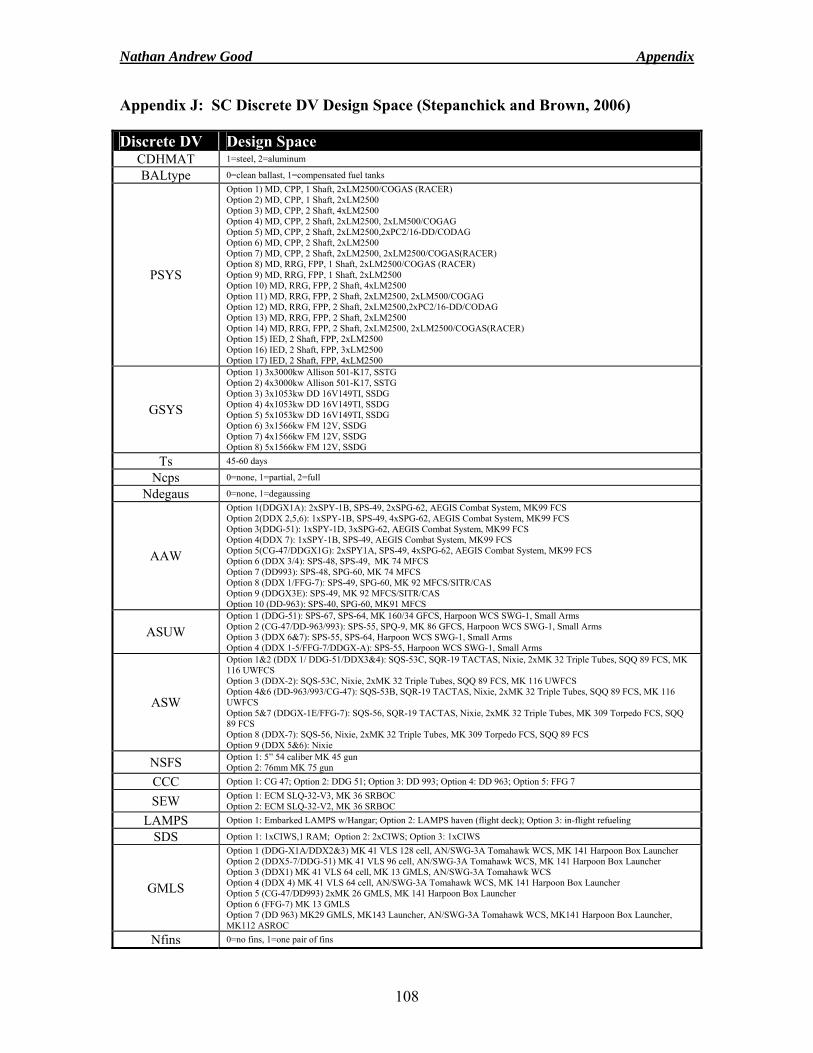
Nathan Andrew Good Appendix
108
Appendix J: SC Discrete DV Design Space (Stepanchick and Brown, 2006)
Discrete DV Design Space CDHMAT 1=steel, 2=aluminum
BALtype 0=clean ballast, 1=compensated fuel tanks
PSYS
Option 1) MD, CPP, 1 Shaft, 2xLM2500/COGAS (RACER) Option 2) MD, CPP, 1 Shaft, 2xLM2500 Option 3) MD, CPP, 2 Shaft, 4xLM2500 Option 4) MD, CPP, 2 Shaft, 2xLM2500, 2xLM500/COGAG Option 5) MD, CPP, 2 Shaft, 2xLM2500,2xPC2/16-DD/CODAG Option 6) MD, CPP, 2 Shaft, 2xLM2500 Option 7) MD, CPP, 2 Shaft, 2xLM2500, 2xLM2500/COGAS(RACER) Option 8) MD, RRG, FPP, 1 Shaft, 2xLM2500/COGAS (RACER) Option 9) MD, RRG, FPP, 1 Shaft, 2xLM2500 Option 10) MD, RRG, FPP, 2 Shaft, 4xLM2500 Option 11) MD, RRG, FPP, 2 Shaft, 2xLM2500, 2xLM500/COGAG Option 12) MD, RRG, FPP, 2 Shaft, 2xLM2500,2xPC2/16-DD/CODAG Option 13) MD, RRG, FPP, 2 Shaft, 2xLM2500 Option 14) MD, RRG, FPP, 2 Shaft, 2xLM2500, 2xLM2500/COGAS(RACER) Option 15) IED, 2 Shaft, FPP, 2xLM2500 Option 16) IED, 2 Shaft, FPP, 3xLM2500 Option 17) IED, 2 Shaft, FPP, 4xLM2500
GSYS
Option 1) 3x3000kw Allison 501-K17, SSTG Option 2) 4x3000kw Allison 501-K17, SSTG Option 3) 3x1053kw DD 16V149TI, SSDG Option 4) 4x1053kw DD 16V149TI, SSDG Option 5) 5x1053kw DD 16V149TI, SSDG Option 6) 3x1566kw FM 12V, SSDG Option 7) 4x1566kw FM 12V, SSDG Option 8) 5x1566kw FM 12V, SSDG
Ts 45-60 days
Ncps 0=none, 1=partial, 2=full
Ndegaus 0=none, 1=degaussing
AAW
Option 1(DDGX1A): 2xSPY-1B, SPS-49, 2xSPG-62, AEGIS Combat System, MK99 FCS Option 2(DDX 2,5,6): 1xSPY-1B, SPS-49, 4xSPG-62, AEGIS Combat System, MK99 FCS Option 3(DDG-51): 1xSPY-1D, 3xSPG-62, AEGIS Combat System, MK99 FCS Option 4(DDX 7): 1xSPY-1B, SPS-49, AEGIS Combat System, MK99 FCS Option 5(CG-47/DDGX1G): 2xSPY1A, SPS-49, 4xSPG-62, AEGIS Combat System, MK99 FCS Option 6 (DDX 3/4): SPS-48, SPS-49, MK 74 MFCS Option 7 (DD993): SPS-48, SPG-60, MK 74 MFCS Option 8 (DDX 1/FFG-7): SPS-49, SPG-60, MK 92 MFCS/SITR/CAS Option 9 (DDGX3E): SPS-49, MK 92 MFCS/SITR/CAS Option 10 (DD-963): SPS-40, SPG-60, MK91 MFCS
ASUW Option 1 (DDG-51): SPS-67, SPS-64, MK 160/34 GFCS, Harpoon WCS SWG-1, Small Arms Option 2 (CG-47/DD-963/993): SPS-55, SPQ-9, MK 86 GFCS, Harpoon WCS SWG-1, Small Arms Option 3 (DDX 6&7): SPS-55, SPS-64, Harpoon WCS SWG-1, Small Arms Option 4 (DDX 1-5/FFG-7/DDGX-A): SPS-55, Harpoon WCS SWG-1, Small Arms
ASW
Option 1&2 (DDX 1/ DDG-51/DDX3&4): SQS-53C, SQR-19 TACTAS, Nixie, 2xMK 32 Triple Tubes, SQQ 89 FCS, MK 116 UWFCS Option 3 (DDX-2): SQS-53C, Nixie, 2xMK 32 Triple Tubes, SQQ 89 FCS, MK 116 UWFCS Option 4&6 (DD-963/993/CG-47): SQS-53B, SQR-19 TACTAS, Nixie, 2xMK 32 Triple Tubes, SQQ 89 FCS, MK 116 UWFCS Option 5&7 (DDGX-1E/FFG-7): SQS-56, SQR-19 TACTAS, Nixie, 2xMK 32 Triple Tubes, MK 309 Torpedo FCS, SQQ 89 FCS Option 8 (DDX-7): SQS-56, Nixie, 2xMK 32 Triple Tubes, MK 309 Torpedo FCS, SQQ 89 FCS Option 9 (DDX 5&6): Nixie
NSFS Option 1: 5” 54 caliber MK 45 gun Option 2: 76mm MK 75 gun
CCC Option 1: CG 47; Option 2: DDG 51; Option 3: DD 993; Option 4: DD 963; Option 5: FFG 7
SEW Option 1: ECM SLQ-32-V3, MK 36 SRBOC Option 2: ECM SLQ-32-V2, MK 36 SRBOC
LAMPS Option 1: Embarked LAMPS w/Hangar; Option 2: LAMPS haven (flight deck); Option 3: in-flight refueling
SDS Option 1: 1xCIWS,1 RAM; Option 2: 2xCIWS; Option 3: 1xCIWS
GMLS
Option 1 (DDG-X1A/DDX2&3) MK 41 VLS 128 cell, AN/SWG-3A Tomahawk WCS, MK 141 Harpoon Box Launcher Option 2 (DDX5-7/DDG-51) MK 41 VLS 96 cell, AN/SWG-3A Tomahawk WCS, MK 141 Harpoon Box Launcher Option 3 (DDX1) MK 41 VLS 64 cell, MK 13 GMLS, AN/SWG-3A Tomahawk WCS Option 4 (DDX 4) MK 41 VLS 64 cell, AN/SWG-3A Tomahawk WCS, MK 141 Harpoon Box Launcher Option 5 (CG-47/DD993) 2xMK 26 GMLS, MK 141 Harpoon Box Launcher Option 6 (FFG-7) MK 13 GMLS Option 7 (DD 963) MK29 GMLS, MK143 Launcher, AN/SWG-3A Tomahawk WCS, MK141 Harpoon Box Launcher, MK112 ASROC
Nfins 0=no fins, 1=one pair of fins
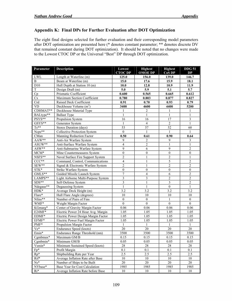
Nathan Andrew Good Appendix
109
Appendix K: Final DPs for Further Evaluation after DOT Optimization
The eight final designs selected for further evaluation and their corresponding model parameters after DOT optimization are presented here (* denotes constant parameter; ** denotes discrete DV that remained constant during DOT optimization). It should be noted that no changes were made to the Lowest CTOC DP or the Universal “Best” DP through DOT optimization.
Parameter Description Lowest CTOC DP
Highest OMOE DP
Highest CoS DP
DDG 51 DP
LWL Length at Waterline (m) 125.0 156.0 139.0 146.7 B Beam at Waterline (m) 15.0 17.6 15.9 18.1 D10 Hull Depth at Station 10 (m) 10.0 12.8 10.9 11.9 T Design Draft (m) 5.0 5.9 5.1 5.7 Cp Prismatic Coefficient 0.600 0.565 0.665 0.612 Cx Maximum Section Coefficient 0.780 0.803 0.877 0.827 Crd Raised Deck Coefficient 0.91 0.70 0.93 0.79 VD Deckhouse Volume (m3) 3400 4600 4400 5200 CDHMAT** Deckhouse Material Type 1 2 1 1 BALtype** Ballast Type 1 1 1 1 PSYS** Propulsion System 16 16 17 3 GSYS** Generator System 1 4 2 1 Ts** Stores Duration (days) 53 57 52 60 Ncps** Collective Protection System 0 1 1 1 CMan Manning Reduction Factor 0.50 0.61 0.90 0.64 AAW** Anti-Air Warfare System 9 2 9 3 ASUW** Anti-Surface Warfare System 4 2 1 1 ASW** Anti-Submarine Warfare System 9 6 9 2 MCM* Mine Countermeasures System 0 0 0 0 NSFS** Naval Surface Fire Support System 2 1 2 1 CCC** Command, Control, Communications 4 1 5 2 SEW** Signal & Electronic Warfare System 2 1 2 2 STK* Strike Warfare System 0 0 0 0 GMLS** Guided Missile Launch System 7 4 6 2 LAMPS** Light Airborne Multi-Purpose System 3 3 2 2 SDS** Self-Defense System 3 1 3 2 Ndegaus** Degaussing System 1 1 0 1 HDK* Average Deck Height (m) 3.2 3.2 3.2 3.2 Flare* Hull Flare Angle (degrees) 10 10 10 10 Nfins** Number of Pairs of Fins 0 0 1 0 WMF* Weight Margin Factor 0 0 0 0 KGmarg* Center of Gravity Margin Factor 0.06 0.06 0.06 0.06 E24MF* Electric Power 24 Hour Avg. Margin 1.05 1.05 1.05 1.05 EDMF* Electric Power Design Margin Factor 1.05 1.05 1.05 1.05 EFMF* Electric Power Fuel Margin Factor 1.05 1.05 1.05 1.05 PMF* Propulsion Margin Factor 1 1 1 1 Ve* Endurance Speed (knots) 20 20 20 20 Emin* Endurance Range Threshold (nm) 3500 3500 3500 3500 Cgmbmax* Maximum GM/B 0.15 0.15 0.15 0.15 Cgmbmin* Minimum GM/B 0.05 0.05 0.05 0.05 Vsmin* Minimum Sustained Speed (knots) 28 28 28 28 Fp* Profit Margin 0.1 0.1 0.1 0.1 Rp* Shipbuilding Rate per Year 2.5 2.5 2.5 2.5 Rif* Average Inflation Rate after Base 10 10 10 10 Ns* Number of Ships to be Built 20 20 20 20 NYbase* Base Year for Cost Calculation 1985 1985 1985 1985 Ri* Average Inflation Rate before Base 10 10 10 10
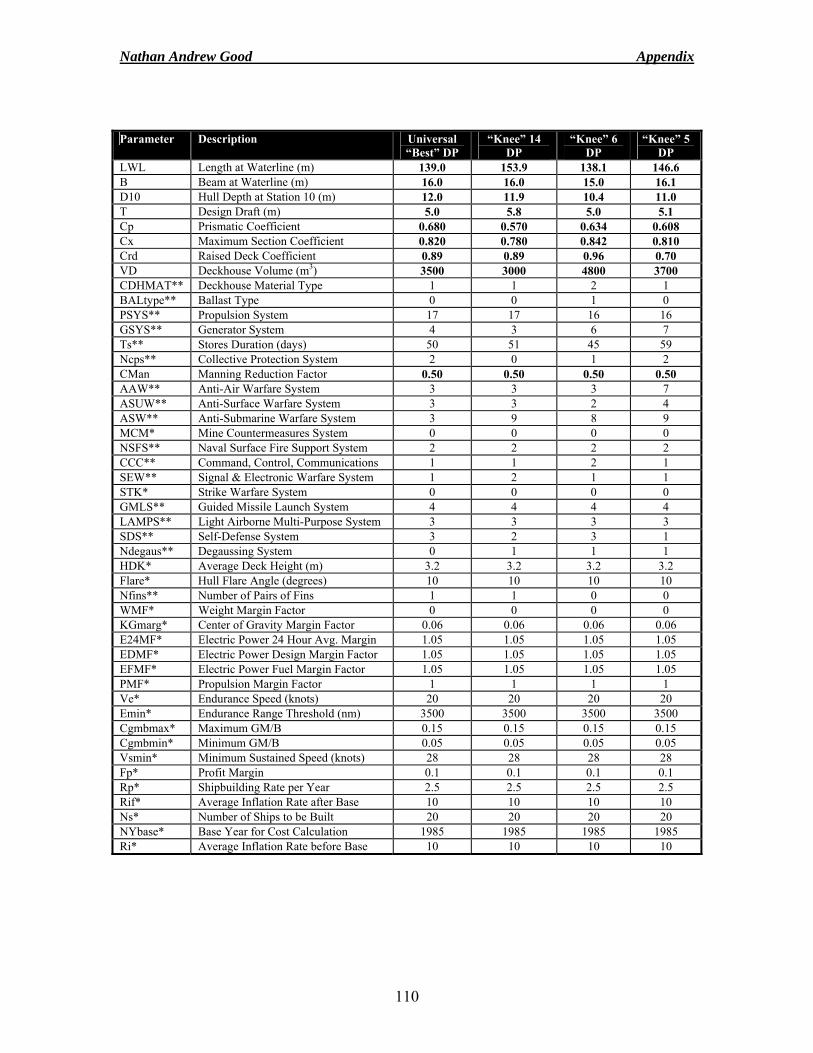
Nathan Andrew Good Appendix
110
Parameter Description Universal “Best” DP
“Knee” 14 DP
“Knee” 6 DP
“Knee” 5 DP
LWL Length at Waterline (m) 139.0 153.9 138.1 146.6 B Beam at Waterline (m) 16.0 16.0 15.0 16.1 D10 Hull Depth at Station 10 (m) 12.0 11.9 10.4 11.0 T Design Draft (m) 5.0 5.8 5.0 5.1 Cp Prismatic Coefficient 0.680 0.570 0.634 0.608 Cx Maximum Section Coefficient 0.820 0.780 0.842 0.810 Crd Raised Deck Coefficient 0.89 0.89 0.96 0.70 VD Deckhouse Volume (m3) 3500 3000 4800 3700 CDHMAT** Deckhouse Material Type 1 1 2 1 BALtype** Ballast Type 0 0 1 0 PSYS** Propulsion System 17 17 16 16 GSYS** Generator System 4 3 6 7 Ts** Stores Duration (days) 50 51 45 59 Ncps** Collective Protection System 2 0 1 2 CMan Manning Reduction Factor 0.50 0.50 0.50 0.50 AAW** Anti-Air Warfare System 3 3 3 7 ASUW** Anti-Surface Warfare System 3 3 2 4 ASW** Anti-Submarine Warfare System 3 9 8 9 MCM* Mine Countermeasures System 0 0 0 0 NSFS** Naval Surface Fire Support System 2 2 2 2 CCC** Command, Control, Communications 1 1 2 1 SEW** Signal & Electronic Warfare System 1 2 1 1 STK* Strike Warfare System 0 0 0 0 GMLS** Guided Missile Launch System 4 4 4 4 LAMPS** Light Airborne Multi-Purpose System 3 3 3 3 SDS** Self-Defense System 3 2 3 1 Ndegaus** Degaussing System 0 1 1 1 HDK* Average Deck Height (m) 3.2 3.2 3.2 3.2 Flare* Hull Flare Angle (degrees) 10 10 10 10 Nfins** Number of Pairs of Fins 1 1 0 0 WMF* Weight Margin Factor 0 0 0 0 KGmarg* Center of Gravity Margin Factor 0.06 0.06 0.06 0.06 E24MF* Electric Power 24 Hour Avg. Margin 1.05 1.05 1.05 1.05 EDMF* Electric Power Design Margin Factor 1.05 1.05 1.05 1.05 EFMF* Electric Power Fuel Margin Factor 1.05 1.05 1.05 1.05 PMF* Propulsion Margin Factor 1 1 1 1 Ve* Endurance Speed (knots) 20 20 20 20 Emin* Endurance Range Threshold (nm) 3500 3500 3500 3500 Cgmbmax* Maximum GM/B 0.15 0.15 0.15 0.15 Cgmbmin* Minimum GM/B 0.05 0.05 0.05 0.05 Vsmin* Minimum Sustained Speed (knots) 28 28 28 28 Fp* Profit Margin 0.1 0.1 0.1 0.1 Rp* Shipbuilding Rate per Year 2.5 2.5 2.5 2.5 Rif* Average Inflation Rate after Base 10 10 10 10 Ns* Number of Ships to be Built 20 20 20 20 NYbase* Base Year for Cost Calculation 1985 1985 1985 1985 Ri* Average Inflation Rate before Base 10 10 10 10