Multi-Document Summarizationand Semantic Relatedness

OLOF MOGREN

Department of Computer Science and EngineeringCHALMERS UNIVERSITY OF TECHNOLOGYUNIVERSITY OF GOTHENBURGGothenburg, Sweden 2015

THESIS FOR THE DEGREE OF LICENTIATE OF ENGINEERING

Multi-Document Summarizationand Semantic Relatedness

OLOF MOGREN

Department of Computer Science and EngineeringCHALMERS UNIVERSITY OF TECHNOLOGY

UNIVERSITY OF GOTHENBURG

Gothenburg, Sweden 2015

Multi-Document Summarizationand Semantic RelatednessOLOF MOGREN

c© OLOF MOGREN, 2015

Thesis for the degree of Licentiate of EngineeringISSN 1652-876XTechnical Report No. 140LDepartment of Computer Science and Engineering

Department of Computer Science and EngineeringChalmers University of Technology and University of GothenburgSE-412 96 GothenburgSwedenTelephone: +46 (0)31-772 1000

Cover:Extractive Multi-Document Summarization; choosing the sentences that are most repre-sentative and informative in a set of input documents.

Chalmers ReproserviceGothenburg, Sweden 2015

To Sofie, Tove, and Stina.

Abstract

Automatic summarization is the process of presenting the contents of written documentsin a short, comprehensive fashion. Many approaches have been proposed for this problem,some of which extract content from the input documents (extractive methods), and othersthat generate the language in the summary based on some representation of the documentcontents (abstractive methods).

This thesis is concerned with extractive summarization in the multi-document setting,and we define the problem as choosing the most informative sentences from the inputdocuments, while minimizing the redundancy in the summary. This definition calls fora way of measuring the similarity between sentences that captures as much as possibleof the meaning. We present novel ways of measuring the similarity between sentences,based on neural word embeddings and sentiment analysis. We also show that combiningmultiple sentence similarity scores, by multiplicative aggregation, helps in the process ofcreating better extractive summaries.

We also discuss the use of information extraction for improving the quality of automaticsummarization by providing ways of assessing the salience of information elements, aswell as helping with the fluency of the output and providing the temporal dimension.

Furthermore, we present graph-based algorithms for clustering words by co-occurrence,and for summarizing short online user-reviews by computing bicliques. The bicliquealgorithm provides a fast, simple algorithm for summarization in many e-commercesettings.

Acknowledgements

I would like to thank both my supervisor Peter Damaschke and my co-supervisorDevdatt Dubhashi, for interesting discussions and inspiring ideas.

A deep thank you also goes to my office-mate and co-author Mikael Kageback; thisthesis would not be much without your contributions and discussions. Thank youFredrik Johansson, for inspiring chats and a creative atmosphere. Also, thank youNina Tahmasebi for teaching me lots of important things, Jonatan Bengtsson for nicework on sentence similarity measures, and Richard Johansson for great advice andinteresting discussions.

Thank you mum and dad for always encouraging me and believing in me, and mybrother and my sisters for supporting, inspiring and challenging me from day one. I wouldnever have made it here without you. Many others have been a great help to me duringthis time. Thank you all!

List of publications

This thesis is based on the following manuscripts.

Paper I

M. Kageback et al. (2014). “Extractive Summarization using Contin-uous Vector Space Models”. Proceedings of The Second Workshop ofContinuous Vector Space Models and their Compositionality, pp. 31–39

Paper IIO. Mogren, M. Kageback, and D. Dubhashi (2015). “ExtractiveSummarization by Aggregating Multiple Similarities”. Proceedings ofRecent Advances in Natural Language Processing, pp. 451–457

Paper IIIN. Tahmasebi et al. (2015). Visions and open challenges for aknowledge-based culturomics. International Journal on Digital Li-braries 15.2-4, 169–187

Paper IVP. Damaschke and O. Mogren (2014). Editing Simple Graphs. Journalof Graph Algorithms and Applications, Special Issue of selected papersfrom WALCOM 2014 18.4, 557–576. doi: 10.7155/jgaa.00337

Paper V

A. S. Muhammad, P. Damaschke, and O. Mogren (2016). “Summariz-ing Online User Reviews Using Bicliques”. Proceedings of The 42ndInternational Conference on Current Trends in Theory and Practiceof Computer Science, SOFSEM, LNCS

Contribution summary

Paper II implemented the submodular optimization algorithm for sentenceselection and created the setup for the experimental evaluation. Ialso wrote parts of the manuscript and made some illustrations.

Paper III am the main author of this work. I designed the study, performedthe experiments, and wrote the manuscript.

Paper IIII wrote section 5, titled ”Temporal Semantic Summarization”, whereI shared my views on possible research directions on generic multi-document summarization.

Paper IVI contributed to the study and the analysis, and to the writing of themanuscript, including making the illustrations.

Paper VI contributed to the study, did a substantial part of the experimentalwork, and contributed to the writing of the manuscript.

Contents

Abstract i

Acknowledgements iii

List of publications v

Contribution summary vii

Contents ix

I Extended summary 1

1 Introduction 3

2 Background 52.1 Semantic Relatedness . . . . . . . . . . . . . . . . . . . . . . . . . . . . . . . 62.2 Measuring Similarity Between Language Units . . . . . . . . . . . . . . . . . 62.3 Automatic Document Summarization . . . . . . . . . . . . . . . . . . . . . . 72.4 Submodular Optimization . . . . . . . . . . . . . . . . . . . . . . . . . . . . . 82.5 Other Approaches to Summarization . . . . . . . . . . . . . . . . . . . . . . . 92.6 Evaluating Automatic Summarization Systems . . . . . . . . . . . . . . . . . 9

3 Multi-Document Summarization and Semantic Relatedness 113.1 Extractive Summarization using Continuous Vector Space Representations . . 123.2 Extractive Summarization by Aggregating Multiple Similarities . . . . . . . . 133.3 Visions and Open Challenges for a Knowledge–Based Culturomics . . . . . . 143.4 Editing Simple Graphs . . . . . . . . . . . . . . . . . . . . . . . . . . . . . . . 153.5 Summarizing Online User Reviews by Computing Bicliques . . . . . . . . . . 16

4 Conclusions 17

References 17

II Publications 21

Part I

Extended summary

Chapter 1

Introduction

Automatic summarization is the process of presenting written documents in a condensedform. This is an active and exciting area of research, but also a highly relevant technologyfor making information easily available to people who struggle with information overload,or need to skim through massive amounts of text in the search of some particular piece ofinformation.

In a very coarse-grained fashion, automatic summarization approaches can be dividedinto two different categories: abstractive and extractive. While abstractive summarizationsystems build some representation of the contents before generating the summary output,extractive systems select parts (typically sentences) of the input documents to present tothe reader This thesis will focus on the latter category. In both, some form of optimizationis normally performed, after stating an objective that gives a score of the output quality.

What is being optimized is at the core of this thesis. A natural way to state the objectiveis to say that we want the summary to have a high similarity to the input documents, andat the same time to have as little redundancy as possible. Many systems that have scoredwell in evaluations measure this similarity by counting word overlaps between sentences.In this thesis, we study ways to make the summaries more semantically aware by usingideas and techniques from deep learning, information extraction and sentiment analysis.

While the focus will be on multi-document summarization, many of the insights willbe applicable to other problems in natural language processing (NLP), such as machinetranslation and semantic relatedness.

The thesis is divided into the following chapters: Chapter 2 presents some of theexisting approaches to summarization that have been proposed as of today, and discussessome of the subtasks that have been considered. Chapter 3 provides a summary of thecontributions in this thesis, while Chapter 4 concludes the work.

This work has mainly been done within the project “Data-driven secure businessintelligence”, grant IIS11-0089 from the Swedish Foundation for Strategic Research (SSF).Parts of the work has also been done within the projects “Algorithms for Inference” and“Towards a knowledge-based culturomics” supported by the Swedish Research Council(2012–2016; dnr 2012-5738).

3

4

Chapter 2

Background

The objective of automatic summarization is to capture the most important topics in aset of documents, and to present them briefly in a manner that is coherent and easy toconsume. We will see how this can be broken down into subproblems in the followingsections, discuss the relationship to semantic relatedness in Sections 2.1–2.2, then surveysome existing methods for automatic document summarization in Sections 2.3–2.5, andconclude the background chapter in Section 2.6 with a discussion about existing techniquesfor summarization evaluation. All summarization approaches discussed here share theaim that the resulting summary has a high similarity with the input documents, and thatit is short and non-redundant at the same time.

Many other NLP applications share parts of this objective, and could benefit fromhaving more meaningful representations. One of them is machine translation, where thegenerated output should capture the semantics of the input, i.e. it should be semanticallysimilar although expressed in a different language, and hence being lexicographicallydissimilar. A different related application is textual entailment, the problem of decidingwhether a sentence follows logically from another sentence.

In order to compute a summary that has a high semantic similarity to a set ofdocuments D, one could envision an automatic summarizer that has a way of interpreting(and representing) the semantics of the content of D. This is however one of the moredifficult problems within artificial intelligence, and so far, we attack it by doing thesimplifications of measuring similarity between language units. In the following sections,we survey existing methods of measuring similarity in language, and existing approachesto summarization. In Chapter 3 we will present solutions to some of the shortcomings ofexisting methods, discuss how a sentence similarity score can capture as much semanticsas possible, and how to best use the similarity scores to extract good sentences for asummary.

5

2.1 Semantic Relatedness

Semantic relatedness between two language units is a measure of how related theirmeanings are. In NLP settings, this is normally defined on the level of words or phrases.

Example: The phrase “riding a bike” is more semantically related to “driving a car”than to “playing a game”. This is easy to see for a human using just intuition (and someknowledge about the language involved), but a more involved problem for a computerprogram.

The SemEval 2014 task 1 for semantic relatedness was defined as predicting a related-ness score for pairs of sentences in English, the score ranging from 1 (completely unrelated)to 5 (highly related). For this, the SICK dataset was presented. Different approacheshave been proposed for this task, from ontology-based to distributional representations.(Zhao, Zhu, and Lan 2014) presented a hybrid approach to the semantic similarity task,while (Tai, Socher, and Manning 2015) proposed a variant of the LSTM recurrent neuralnetwork architecture, where the LSTM modules are arranged according to a parse tree.

Semantic similarity is stricter than semantic relatedness, as it only includes the “is a”relationship (while relatedness includes any semantic relations). We will not go more intothe distinction here, as it is not a focus of this thesis, and much literature use the twoterms interchangeably.

Example: A bicycle is highly semantically related to a wheel, but they are notsimilar, neither semantically nor lexicographically. Conversely, “driving someone crazy”is lexicographically similar to “driving a car” but there is no apparent semantic similarityneither any semantic relatedness.

2.2 Measuring Similarity Between Language Units

Falling short of being able to understand and represent the semantic content in a text,one typically let computers use more shallow ways of relating different texts to eachother. On character level, the edit-distance (Levenshtein 1966) gives a measure on howsimilar two strings of text are. On word-level, word overlap scores are another class ofsimilarity measures that have been successfully used in summarization systems. Severaldifferent variants of such scores have been proposed in the summarization literature, withdifferences in preprocessing (such as stop-words removal, spelling corrections, and otherfiltering), weighting schemes, and normalization.

All similarity measures in this category are surface matching techniques, there is nosemantical information used.

6

In 2011, H. Lin and Bilmes used a vector representation for each sentence, defined as itsbag-of-terms representation, weighted by TFIDF (where terms are unigrams and bigrams).The similarity of each pair of sentences were then scored by the cosine similarity:

Msi,sj =

∑w∈si

tfw,i · tfw,j · idf2w√∑w∈si

tfw,siidf2w

√∑w∈sj

tfw,sj idf2w

A similar representation was also used by Radev et al. (2004).Mihalcea and Tarau used a similar approach (2004), without the TFIDF weighting,

and with a different normalization:

Msi,sj = |si ∩ sj |/(log |si|+ log |sj |)

In their master’s thesis, Bengtsson and Skeppstedt survey the landscape of similaritymeasures, including the ones mentioned in this section, and evaluate them together withTextRank, an existing summarization system (see Section 2.5).

2.3 Automatic Document Summarization

Automatic document summarization is the problem of presenting the most importantcontent of a set of input documents. Methods for solving this can be classified as eitherabstractive or extractive. The former represents systems that process the input and thengenerate the language in the resulting summary, and the latter represents systems thatchoose parts (typically whole sentences) from the input documents and extract those, intheir current form, to constitute the summary.

In this thesis we will focus on extractive systems, which date back to 1958, when Luhnpresented an algorithm that looked at words’ frequencies of occurring in a document.Luhn identified words as important for the document if they appeared not too commonlyand not too rarely, and then scored sentences with a formula depending on the number ofimportant words in them.

The idea of determining the importance of words has lived on, but threshold valueshave been replaced with other approaches, such as TFIDF weighting1, and regressionmodels (Hong and Nenkova 2014). Both of these make away with the hard constraints ofthreshold values, and instead provide a continuous measure of importance for differentterms.

1TFIDF, Term frequency times inverse document frequency, gives high weight to words that arespecific to this document

7

Figure 2.4.1: Illustration of a monotonically non-decreasing, submodular set function F .The left bowl contains a subset (S) of the objects in the right bowl (T ). Let F be thenumber of different shapes in a bowl. The value of F changes at least as much whenadding an object to S (left), compared to adding it to T (right). Adding a ball to a bowlwith only triangles and squares increases the number of shapes, but adding it to a bowlwith all three shapes does not.

2.4 Submodular Optimization

One of the most successful extractive summarization systems was presented in (H. Linand Bilmes 2011). Here, a summary is seen as a set of sentences, and the quality of asummary is scored with a function measuring its coverage (with regards to the inputdocuments) and diversity (internally). The coverage and the diversity is defined based ona similarity measure between sentences. They showed that their set scoring function issubmodular, which allows for a greedy approximation algorithm. The resulting system isfast and obtained good results in evaluations, that are still on-par with state-of-the-art.

A set function F is a function that has subsets of some universe U as its domain.Here we will consider only real-valued set functions. A (monotonically non-decreasing)submodular set function is a real-valued set function that obeys the principle of diminishingreturns. Intuitively, this means that adding an element v to a small set S increases thefunction value more than adding the same element to a bigger set.

Formally, if S ⊆ T ⊆ U\v, then

F(S + v)−F(S) ≥ F(T + v)−F(T ).

Maximizing monotone non-decreasing submodular set functions can be done with asimple greedy algorithm, which yields a (1− 1

e ) ≈ 0.63 approximation.The objective functions of many approaches for extractive summarization have been

shown to be submodular.

8

2.5 Other Approaches to Summarization

In TextRank (Mihalcea and Tarau 2004) a document is represented as a graph where eachsentence is denoted by a vertex and pairwise similarities between sentences are representedby edges with a weight corresponding to a word-overlap similarity between the sentences.The PageRank ranking algorithm is used on this graph to estimate the importance ofdifferent sentences. Classy 04 (Conroy et al. 2004) was the best performing system in theofficial DUC 2004 evaluations. After some linguistic preprocessing, they used a HiddenMarkov Model with a mutual information score based on “signature tokens”, tokens thatare more likely to occur in the input document than in the rest of the corpus. ISCI (Gillick,Favre, and Hakkani-Tur 2008) optimized coverage of key bigrams, using integer linearprogramming. (Kulesza and Taskar 2012) presented the use of Determinantal PointProcesses for summarization, a probabilistic formulation that allows for a balance betweendiversity and coverage. Occams V (Davis, Conroy, and Schlesinger 2012) is a system usinglatent semantic analysis and a sentence selection algorithm based on budgeted maximumcoverage and knapsack. (Hong and Nenkova 2014) presented RegSum, a supervisedlogistic regression model for predicting word importance based on engineered features.Using these weights they presented an extractive summarizer that performed well andgave insight in word categories that are important for summary extraction. (Bonzanini,Martinez-Alvarez, and Roelleke 2013) presented an iterative procedure that removedredundant sentences from the input documents, until a sufficiently short summary wasobtained. The system performed well in the evaluations on short online user reviews.

2.6 Evaluating Automatic Summarization Systems

Assessing the quality of summaries is an active area of research, and it is not entirelyunlike the process of producing actual summaries, as the existing approaches have focusedon scoring a summary for its similarity to a gold-standard written by human experts.

The NIST Document Understanding Conferences (DUC), was a conference witha competition for the summarization task. In 2008, it was superseded by the TextUnderstanding Conferences (TAC), and continued as a track in the new conference. Thedataset from DUC 2004 has lived on as the standard benchmark dataset for genericmulti-document summarization. It consists of 50 document clusters, each comprisingaround ten news articles (between 149 and 590 sentences each) and accompanied withfour gold-standard summaries created by manual experts.

The Opinosis dataset (Ganesan, Zhai, and Han 2010) contains short online user-reviewsfor 51 different topics. Each topic contains between 50 and 575 sentences of reviews madeby different authors about a certain characteristic of a hotel, car, or a product. As onlineuser-reviews typically are not authored by professional writers, the quality of the text islower, and it contains more opinionated sentences.

In DUC, a series of different approaches for evaluation have been used through theyears in different combinations.

Initially, the evaluation of the systems participating in the competition were evaluatedmanually. This is of course a tedious task and a solution that doesn’t scale well.

9

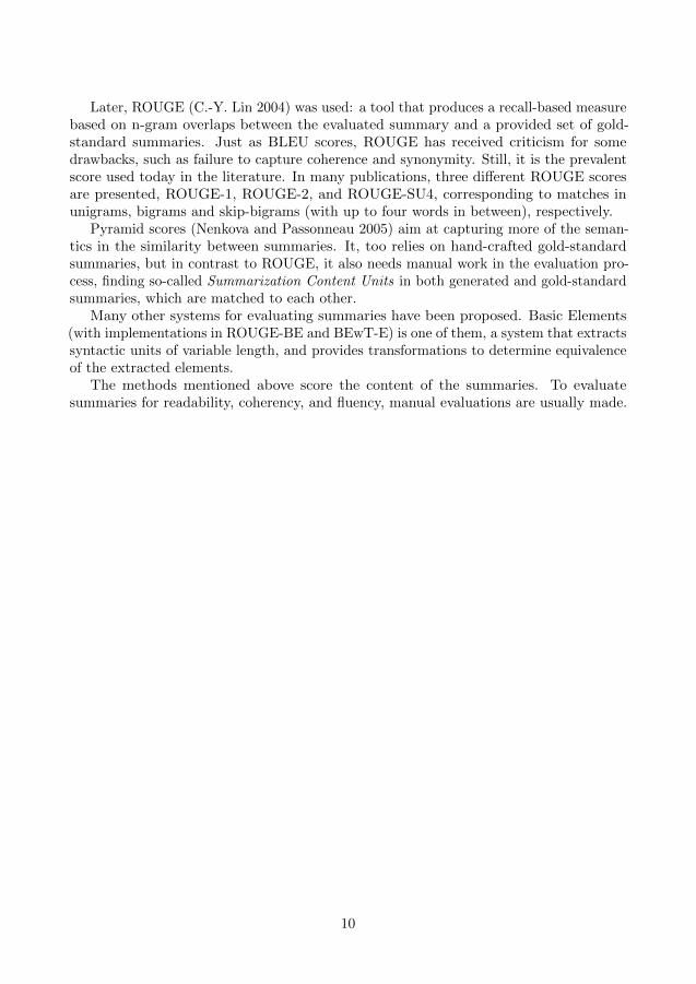
Later, ROUGE (C.-Y. Lin 2004) was used: a tool that produces a recall-based measurebased on n-gram overlaps between the evaluated summary and a provided set of gold-standard summaries. Just as BLEU scores, ROUGE has received criticism for somedrawbacks, such as failure to capture coherence and synonymity. Still, it is the prevalentscore used today in the literature. In many publications, three different ROUGE scoresare presented, ROUGE-1, ROUGE-2, and ROUGE-SU4, corresponding to matches inunigrams, bigrams and skip-bigrams (with up to four words in between), respectively.

Pyramid scores (Nenkova and Passonneau 2005) aim at capturing more of the seman-tics in the similarity between summaries. It, too relies on hand-crafted gold-standardsummaries, but in contrast to ROUGE, it also needs manual work in the evaluation pro-cess, finding so-called Summarization Content Units in both generated and gold-standardsummaries, which are matched to each other.

Many other systems for evaluating summaries have been proposed. Basic Elements(with implementations in ROUGE-BE and BEwT-E) is one of them, a system that extractssyntactic units of variable length, and provides transformations to determine equivalenceof the extracted elements.

The methods mentioned above score the content of the summaries. To evaluatesummaries for readability, coherency, and fluency, manual evaluations are usually made.

10

Chapter 3

Multi-DocumentSummarization and SemanticRelatedness

The following sections will outline the main contributions of this thesis.Chapter 2 surveyed previous work on extractive summarization, and described that

most summarization techniques rely on measuring similarity between language units,such as sentences. In this chapter, we will build on these ideas, and propose ways tomeasure sentence similarity that capture more semantic information, using ideas fromword embeddings and sentiment analysis.

In Section 3.1, we show how summaries can be computed by using word embeddingsto compute the sentence similarity score, in Section 3.2 we build on this and show thataggregating several ways of measuring the sentence similarity at the same time helpsto create better extractive summaries. These results are illustrated by incorporatingthe ideas into the existing submodular optimization approach to summarization (seeSection 2.4). Section 3.3 presents some possible ideas for future research, such as usinginformation extraction to improve the performance of summarization systems. The twofinal sections in this chapter takes a slightly different view, approaching NLP problemswith ideas from graph theory. Section 3.4 discusses the complexity of finding clustersby graph modification. Section 3.5 presents a novel approach to summarizing onlineuser-reviews based on detecting bicliques in the bipartite word-document graph.

11

3.1 Extractive Summarization usingContinuous Vector Space Representations

In the first paper, we present a novel way of utilizing word embeddings for summarization.Word embeddings are representations for words in a vector space. Simple examples

of this are context vectors, where you represent a word w by a vector v that has adimensionality the same as the size of the vocabulary. All components of v are zero,except at indices representing words that have been observed in the context of w. Thiskind of model is called distributional, and it naturally encodes distributional similarities.The resulting representations are however very high-dimensional and sparse.

In contrast, the word embeddings that we consider in this paper are continuous vectorspace representations of much lower dimension (hence, they are also denser). This classof word embeddings are also known as distributed representations, and they typicallyuse (or at least are inspired by) artificial neural networks for training. They are alsodistributional representations, as they encode similar words close in the vector space.Collobert and Weston (2008) trained the representations using a neural network in amultitask training scenario. In the Word2Vec Skip-Gram model (Mikolov, Chen, et al.2013), the vectors are obtained by training a model to predict the context words. TheGloVe model is trained using global word co-occurrence statistics (Pennington, Socher,and Manning 2014). Vectors from the models mentioned above have been shown to encodemany semantic aspects of words. This shows as relations between the correspondingvectors; e.g. the difference between the vectors for a country and its capital is almostconstant over different countries:

vStockholm − vSweden ≈ vBerlin − vGermany

We use the word embeddings to capture more semantics in the sentence similarityscore. To be able to easily compare two sentences, we first create a sentence representationof fixed dimension for each sentence. We evaluate two different ways of doing this:simple vector addition (Mikolov, Sutskever, et al. 2013) and recursive auto-encoders(RAE) (Socher et al. 2011).

An RAE is an auto-encoder: a feed forward neural network that is trained to reconstructthe input at its output. In an auto-encoder, there is typically a lower-dimensional hiddenlayer, to obtain an amount of compression. A recursive auto-encoder uses the syntacticparse-tree of a sentence, to provide the layout of the auto-encoder network. In this way,intermediate representations are trained recursively for pairs of input representations.The dimensionality is the same after each pairwise input.

In the evaluation, two different word representations are used: those of (Mikolov,Chen, et al. 2013), and (Collobert and Weston 2008). Extending the representations tomore complex structures than words (such as sentences and documents) is an active areaof research.

The experimental evaluation suggests that using continuous vector space models affectsthe resulting summaries favourably, but surprisingly, the simple approach of summingthe vectors to sentence representations outperforms the seemingly more sophisticatedapproach with RAEs.

12

x1

x2

x3

x′1

x′2

x′3

Rootlayer

Inputlayer

Outputlayer

θe θd

Figure 3.1.1: An unfolding recursive auto-encoder. In this example, a three words phrase[x1, x2, x3] is the input. The weight matrix θe is used to encode the compressed represen-tations, while θd is used to decode the representations and reconstruct the sentence.

3.2 Extractive Summarization by AggregatingMultiple Similarities

This paper builds on the approach with word representations (Section 3.1). We alsopresent a sentence similarity score based on sentiment analysis, and show that we cancreate better summaries by combining the word embeddings with the sentiment score andtraditional word-overlap measures, by multiplying the scores together. Using multiplicationcorresponds to a conjunctive aggregation, where all involved similarity scores need tobe high for the resulting score to be high, but only one of them needs to be low for theresulting score to be low. Products of experts have been shown to work well in manyother applications and is a standard way of combining kernels.

It has been shown (Hong and Nenkova 2014) that when human authors create sum-maries for news paper articles, they use negative emotion words at a higher rate. Thismotivated our experiments with sentiment words. We define a new sentence similaritymeasure, comparing the sentiment charge of two sentences. Much as expected, thissentence similarity measure is in itself weak, but when used in aggregation with othersimilarity measures, it can provide an improvement.

We call the resulting system MULTSUM, an automatic summarizer that uses sub-modular optimization with multiplicative aggregation of sentence similarity scores, takingseveral aspects into account when selecting sentences.

Msi,sj =∏

M lsi,sj ,

where M l denotes the different similarity measures used.The resulting summaries are evaluated on DUC 2004; the de-facto standard benchmark

dataset for generic multi-document summarization, and obtain state–of–the–art results.Specifically, the scores where MULTSUM excels, are ROUGE-2 and ROUGE-SU4, withmatches in bigrams and skip-bigrams (with up to four words in between), respectively,suggesting that the resulting summaries have high fluency.

13

president of USA

Barack Obama

capital of

Washington DC

married

Michelle Obama free tra

de agreementCanada

free trade agreement

Mexico

prime minister of

Stephen Harper

producer of iPhone

AppleCEO of

Timothy D. Cook

Samsungcompetitors

Figure 3.3.1: Example of a graph of entities and relations. Entities are of different types,and are represented by nodes in the graph. The edges corresponds to (different kinds of)relations between entities.

3.3 Visions and Open Challenges for a Knowledge–Based Culturomics

In this white paper we discuss automatic summarization in the setting of historical texts,and present ideas for making automatic summaries more aware of what is important in thetext. Information extraction (IE) is the process of extracting entities, relations, and eventsfrom the text. The extracted information would be used as a first step in a summarizationsystem to improve the information content in the summaries. Previous work has shownthat incorporating IE can improve the results of multi-document summarization (Ji et al.2013).

Entities, relations and events extracted from the documents are used to score sentencesfor extraction; a higher score is given to sentences with salient information units. Fur-thermore, temporal information in the input documents help create summaries that arefluent and keep the narrative. As a continuation of this, one can envision an abstractivesummarization system that incorporates extracted information.

14

Figure 3.3.2: A subset of the word co-occurrence graph generated using data from Wikipedia,using some edge weight threshold t. The visualization is created with Gephi. One canclearly see dense word-clusters forming with only few edges connecting clusters with eachother.

3.4 Editing Simple Graphs

Graph editing is the process of modifying an input graph by operations such as inserting,removing, or reversing edges until some prescribed property of the graph is met. Thispaper discusses the complexity of editing an input graph G, into a graph with a predefinedcritical-clique graph. A clique graph is a representation of the cliques of a graph, and therelationship between them. A critical-clique is an equivalence class defined by verticesthat share the same neighborhood. Consequently, a critical-clique graph has a vertex foreach critical clique, and edges between two vertices if the corresponding cliques in theoriginal graph are connected.

15

The work in this paper is motivated by the wish to find clusters in word-co-occurrencegraphs (see Figure 3.3.2 for a visualization of a word co-occurrence graph from Wikipediadata). Applications for this can be topic modelling or measures of similarity betweenwords. The distributional hypothesis (Harris 1954) states that semantically similar wordsoccur within similar contexts. Hence, the similarity found in this way could be a coarsevariant of the kind of similarity found in word embeddings, and hence usable for the kindof semantic similarity tasks discussed for summarization. Using such clusters however,has been out of the scope of this thesis and is left for future work. The word “simple”in the title refers to the fact that we discuss some simple cases of graphs as the target(critical-clique) graph, corresponding to finding “simple” structures of clusters in theinput graph.

We show that several variants of this problem is in SUBEPT, the complexity classof fixed parameter tractable problems solvable in subexponential time in the parameter(2o(k)). In this case, the parameter k represents the number of edits. Of course, the timecomplexity also depends on the input size n, but only polynomially.

3.5 Summarizing Online User Reviews by ComputingBicliques

In this paper, we approach the problem of extractive summarization for short (onesentence) online user-reviews by considering the bipartite graph of documents and words(for a document vertex v, there is an edge between v and every word included in thecorresponding document). The result is a simple combinatorial algorithm for producingan extractive summary based on bicliques in the document-word graph. A bipartite graphis a graph where the vertices can be divided into two sets, T and W , and edges musthave exactly one endpoint in each of these sets. A bipartite clique, or biclique is a subsetof the vertices in T and W that induces a complete bipartite subgraph (where everyvertex in the first set is connected to every vertex in the second set). We extract bicliqueswhere the number of sentences is two, then score them by the number of words that thesentences share. Thereafter sentences are scored by the number of bicliques they are partof, and finally the most representative sentences are presented as a summary.

The method scores well when compared to other methods on short online user-reviews,and due to a clever way to exploit statistical properties of word-frequencies (they followpower-laws), a very good running time can be obtained in practice.

16

Chapter 4

Conclusions

This thesis has discussed extractive multi-document summarization. Most extractivesummarization systems rely on measuring the similarity of language units (typicallysentences).

We have defined novel ways of measuring the sentence similarity score by leveragingword embeddings and sentiment analysis. When aggregating several similarity scores atthe same time, using element-wise multiplication, our system obtains state–of–the–artresults on standard benchmark datasets.

We have also discussed using information extraction to add temporal information andimprove summarization systems in the setting of historical texts.

Finally, we have proposed graph-based approaches for clustering of words and forextracting sentences for summaries of online user-reviews. We show that both are fast(in the first case, we have a theoretical motivation, in the second case the motivation isbacked by statistical properties of words).

So far, we have only scratched the surface of learning how to construct NLP systemsthat really work on the semantic level. Plenty remains to be done, such as exploring howto best create distributional representations for sentences. Recent work has been studyingdifferent ways to compose word embeddings to create sentence representations (Blacoe andLapata 2012; Hermann and Blunsom 2013). Perhaps an even more promising directionis the use of deep learning and recurrent neural networks (Graves 2013). Such modelshave been successfully used for machine translation (Sutskever, Vinyals, and Le 2014)and could be useful both for extractive and abstractive summarization in an end–to–enddeep learning approach.

17

References

Bengtsson, J. and C. Skeppstedt (2012). “Automatic extractive single document summa-rization”. MA thesis. Chalmers University of Technology and University of Gothenburg.url: http://publications.lib.chalmers.se/records/fulltext/174136/174136.pdf.

Blacoe, W. and M. Lapata (2012). “A Comparison of Vector-based Representations forSemantic Composition”. Proceedings of the 2012 Joint Conference on Empirical Meth-ods in Natural Language Processing and Computational Natural Language Learning.EMNLP-CoNLL ’12. Jeju Island, Korea: Association for Computational Linguistics,pp. 546–556. url: http://dl.acm.org/citation.cfm?id=2390948.2391011.

Bonzanini, M., M. Martinez-Alvarez, and T. Roelleke (2013). “Extractive summarisationvia sentence removal: condensing relevant sentences into a short summary”. SIGIR,pp. 893–896.

Collobert, R. and J. Weston (2008). “A unified architecture for natural language processing:Deep neural networks with multitask learning”. Proceedings of ICML, pp. 160–167.

Conroy, J. M. et al. (2004). “Left-brain/right-brain multi-document summarization”.Proceedings of DUC 2004.

Damaschke, P. and O. Mogren (2014). Editing Simple Graphs. Journal of Graph Algorithmsand Applications, Special Issue of selected papers from WALCOM 2014 18.4, 557–576.doi: 10.7155/jgaa.00337.

Davis, S. T., J. M. Conroy, and J. D. Schlesinger (2012). “OCCAMS–An OptimalCombinatorial Covering Algorithm for Multi-document Summarization”. Data MiningWorkshops (ICDMW). IEEE, pp. 454–463.

Ganesan, K., C. Zhai, and J. Han (2010). “Opinosis: a graph-based approach to abstractivesummarization of highly redundant opinions”. Proceedings of the 23rd InternationalConference on Computational Linguistics. ACL, pp. 340–348.

Gillick, D., B. Favre, and D. Hakkani-Tur (2008). “The icsi summarization system at tac2008”. Proceedings of TAC.

Graves, A. (2013). Generating sequences with recurrent neural networks. arXiv preprintarXiv:1308.0850.

Harris, Z. S. (1954). Distributional structure. Word.Hermann, K. M. and P. Blunsom (2013). “The Role of Syntax in Vector Space Models of

Compositional Semantics.” ACL, pp. 894–904.Hong, K. and A. Nenkova (2014). “Improving the estimation of word importance for news

multi-document summarization”. Proceedings of EACL.

18

Ji, H. et al. (2013). “Open-Domain multi-document summarization via information ex-traction: Challenges and prospects”. Multi-source, Multilingual Information Extractionand Summarization. Springer, pp. 177–201.

Kageback, M. et al. (2014). “Extractive Summarization using Continuous Vector SpaceModels”. Proceedings of The Second Workshop of Continuous Vector Space Modelsand their Compositionality, pp. 31–39.

Kulesza, A. and B. Taskar (2012). Determinantal point processes for machine learning.arXiv:1207.6083.

Levenshtein, V. I. (1966). “Binary codes capable of correcting deletions, insertions, andreversals”. Soviet physics doklady. Vol. 10. 8, pp. 707–710.

Lin, C.-Y. (2004). “Rouge: A package for automatic evaluation of summaries”. TextSummarization Branches Out: Proc. of the ACL-04 Workshop, pp. 74–81.

Lin, H. and J. Bilmes (2011). “A Class of Submodular Functions for Document Summa-rization.” ACL.

Luhn, H. P. (1958). The automatic creation of literature abstracts. IBM Journal 2.2,159–165.

Mihalcea, R. and P. Tarau (2004). “TextRank: Bringing order into texts”. Proceedings ofEMNLP. Vol. 4.

Mikolov, T., K. Chen, et al. (2013). Efficient Estimation of Word Representations inVector Space. arXiv:1301.3781.

Mikolov, T., I. Sutskever, et al. (2013). “Distributed representations of words and phrasesand their compositionality”. Advances in Neural Information Processing Systems,pp. 3111–3119.

Mogren, O., M. Kageback, and D. Dubhashi (2015). “Extractive Summarization byAggregating Multiple Similarities”. Proceedings of Recent Advances in Natural LanguageProcessing, pp. 451–457.

Muhammad, A. S., P. Damaschke, and O. Mogren (2016). “Summarizing Online UserReviews Using Bicliques”. Proceedings of The 42nd International Conference onCurrent Trends in Theory and Practice of Computer Science, SOFSEM, LNCS.

Nenkova, A. and R. J. Passonneau (2005). “Evaluating Content Selection in Summarization:The Pyramid Method.” HLT-NAACL, pp. 145–152. url: http://dblp.uni-trier.de/db/conf/naacl/naacl2004.html#NenkovaP04.

Pennington, J., R. Socher, and C. D. Manning (2014). Glove: Global vectors for wordrepresentation. Proceedings of the Empiricial Methods in Natural Language Processing(EMNLP 2014) 12, 1532–1543.

Radev, D. R. et al. (2004). Centroid-based summarization of multiple documents. Infor-mation Processing & Management 40.6, 919–938.

Socher, R. et al. (2011). “Dynamic Pooling and Unfolding Recursive Autoencoders forParaphrase Detection.” Advances in Neural Information Processing Systems. Vol. 24,pp. 801–809.

Sutskever, I., O. Vinyals, and Q. V. Le (2014). “Sequence to sequence learning with neuralnetworks”. Advances in neural information processing systems, pp. 3104–3112.

Tahmasebi, N. et al. (2015). Visions and open challenges for a knowledge-based culturomics.International Journal on Digital Libraries 15.2-4, 169–187.

19

Tai, K. S., R. Socher, and C. D. Manning (2015). Improved semantic representations fromtree-structured long short-term memory networks. arXiv preprint arXiv:1503.00075.

Zhao, J., T. T. Zhu, and M. Lan (2014). Ecnu: One stone two birds: Ensemble ofheterogenous measures for semantic relatedness and textual entailment. SemEval 2014,271.

20

Part II

Publications

Paper I

Extractive Summarization using Continuous Vector SpaceModels

M. Kageback et al.

Reprinted from Proceedings of The Second Workshop of Continuous Vector Space

Models and their Compositionality, 2014

Extractive Summarization using Continuous Vector Space Models

Mikael Kageback, Olof Mogren, Nina Tahmasebi, Devdatt DubhashiComputer Science & Engineering

Chalmers University of TechnologySE-412 96, Goteborg

{kageback, mogren, ninat, dubhashi}@domain

AbstractAutomatic summarization can help usersextract the most important pieces of infor-mation from the vast amount of text digi-tized into electronic form everyday. Cen-tral to automatic summarization is the no-tion of similarity between sentences intext. In this paper we propose the use ofcontinuous vector representations for se-mantically aware representations of sen-tences as a basis for measuring similar-ity. We evaluate different compositionsfor sentence representation on a standarddataset using the ROUGE evaluation mea-sures. Our experiments show that the eval-uated methods improve the performanceof a state-of-the-art summarization frame-work and strongly indicate the benefitsof continuous word vector representationsfor automatic summarization.

1 Introduction

The goal of summarization is to capture the im-portant information contained in large volumes oftext, and present it in a brief, representative, andconsistent summary. A well written summary cansignificantly reduce the amount of work needed todigest large amounts of text on a given topic. Thecreation of summaries is currently a task best han-dled by humans. However, with the explosion ofavailable textual data, it is no longer financiallypossible, or feasible, to produce all types of sum-maries by hand. This is especially true if the sub-ject matter has a narrow base of interest, either dueto the number of potential readers or the durationduring which it is of general interest. A summarydescribing the events of World War II might forinstance be justified to create manually, while asummary of all reviews and comments regardinga certain version of Windows might not. In suchcases, automatic summarization is a way forward.

In this paper we introduce a novel applicationof continuous vector representations to the prob-lem of multi-document summarization. We evalu-ate different compositions for producing sentencerepresentations based on two different word em-beddings on a standard dataset using the ROUGEevaluation measures. Our experiments show thatthe evaluated methods improve the performance ofa state-of-the-art summarization framework whichstrongly indicate the benefits of continuous wordvector representations for this tasks.

2 Summarization

There are two major types of automatic summa-rization techniques, extractive and abstractive. Ex-tractive summarization systems create summariesusing representative sentences chosen from the in-put while abstractive summarization creates newsentences and is generally considered a more dif-ficult problem.

Figure 1: Illustration of Extractive Multi-Document Summarization.

For this paper we consider extractive multi-document summarization, that is, sentences arechosen for inclusion in a summary from a set ofdocuments D. Typically, extractive summariza-tion techniques can be divided into two compo-nents, the summarization framework and the sim-ilarity measures used to compare sentences. Next

we present the algorithm used for the frameworkand in Sec. 2.2 we discuss a typical sentence sim-ilarity measure, later to be used as a baseline.

2.1 Submodular OptimizationLin and Bilmes (2011) formulated the problem ofextractive summarization as an optimization prob-lem using monotone nondecreasing submodularset functions. A submodular function F on theset of sentences V satisfies the following property:for any A ⊆ B ⊆ V \{v}, F (A+ {v})−F (A) ≥F (B + {v})− F (B) where v ∈ V . This is calledthe diminishing returns property and captures theintuition that adding a sentence to a small set ofsentences (i.e., summary) makes a greater contri-bution than adding a sentence to a larger set. Theaim is then to find a summary that maximizes di-versity of the sentences and the coverage of the in-put text. This objective function can be formulatedas follows:

F(S) = L(S) + λR(S)

where S is the summary, L(S) is the coverage ofthe input text, R(S) is a diversity reward function.The λ is a trade-off coefficient that allows us todefine the importance of coverage versus diversityof the summary. In general, this kind of optimiza-tion problem is NP-hard, however, if the objectivefunction is submodular there is a fast scalable al-gorithm that returns an approximation with a guar-antee. In the work of Lin and Bilmes (2011) a sim-ple submodular function is chosen:

L(S) =∑

i∈Vmin{

∑

j∈SSim(i, j), α

∑

j∈VSim(i, j)}

(1)The first argument measures similarity betweensentence i and the summary S, while the sec-ond argument measures similarity between sen-tence i and the rest of the input V . Sim(i, j) isthe similarity between sentence i and sentence jand 0 ≤ α ≤ 1 is a threshold coefficient. The di-versity reward function R(S) can be found in (Linand Bilmes, 2011).

2.2 Traditional Similarity MeasureCentral to most extractive summarization sys-tems is the use of sentence similarity measures(Sim(i, j) in Eq. 1). Lin and Bilmes measuresimilarity between sentences by representing eachsentence using tf-idf (Salton and McGill, 1986)vectors and measuring the cosine angle between

vectors. Each sentence is represented by a wordvector w = (w1, . . . , wN ) where N is the size ofthe vocabulary. Weights wki correspond to the tf-idf value of word k in the sentence i. The weightsSim(i, j) used in the L function in Eq. 1 are foundusing the following similarity measure.

Sim(i, j) =

∑w∈i

tfw,i × tfw,j × idf2w√∑

w∈itf2w,i × idf2w

√∑w∈j

tf2w,j × idf2w

(2)where tfw,i and tfw,j are the number of occur-

rences of w in sentence i and j, and idfw is theinverse document frequency (idf ) of w.

In order to have a high similarity between sen-tences using the above measure, two sentencesmust have an overlap of highly scored tf-idf words.The overlap must be exact to count towards thesimilarity, e.g, the terms The US President andBarack Obama in different sentences will not addtowards the similarity of the sentences. To cap-ture deeper similarity, in this paper we will inves-tigate the use of continuous vector representationsfor measuring similarity between sentences. In thenext sections we will describe the basics neededfor creating continuous vector representations andmethods used to create sentence representationsthat can be used to measure sentence similarity.

3 Background on Deep Learning

Deep learning (Hinton et al., 2006) is a mod-ern interpretation of artificial neural networks(ANN), with an emphasis on deep network ar-chitectures. Deep learning can be used for chal-lenging problems like image and speech recogni-tion (Krizhevsky et al., 2012; Graves et al., 2013),as well as language modeling (Mikolov et al.,2010), and in all cases, able to achieve state-of-the-art results.

Inspired by the brain, ANNs use a neuron-likeconstruction as their primary computational unit.The behavior of a neuron is entirely controlled byits input weights. Hence, the weights are wherethe information learned by the neuron is stored.More precisely the output of a neuron is computedas the weighted sum of its inputs, and squeezedinto the interval [0, 1] using a sigmoid function:

yi = g(θTi x) (3)

g(z) =1

1 + e−z(4)

x1

x2

x3

x4

y3

Hiddenlayer

Inputlayer

Outputlayer

Figure 2: FFNN with four input neurons, one hid-den layer, and 1 output neuron. This type of ar-chitecture is appropriate for binary classificationof some data x ∈ R4, however depending on thecomplexity of the input, the number and size of thehidden layers should be scaled accordingly.

where θi are the weights associated with neuron iand x is the input. Here the sigmoid function (g) ischosen to be the logistic function, but it may alsobe modeled using other sigmoid shaped functions,e.g. the hyperbolic tangent function.

The neurons can be organized in many differ-ent ways. In some architectures, loops are permit-ted. These are referred to as recurrent neural net-works. However, all networks considered here arenon-cyclic topologies. In the rest of this sectionwe discuss a few general architectures in more de-tail, which will later be employed in the evaluatedmodels.

3.1 Feed Forward Neural NetworkA feed forward neural network (FFNN) (Haykin,2009) is a type of ANN where the neurons arestructured in layers, and only connections to sub-sequent layers are allowed, see Figure 2. The al-gorithm is similar to logistic regression using non-linear terms. However, it does not rely on theuser to choose the non-linear terms needed to fitthe data, making it more adaptable to changingdatasets. The first layer in a FFNN is called theinput layer, the last layer is called the output layer,and the interim layers are called hidden layers.The hidden layers are optional but necessary to fitcomplex patterns.

Training is achieved by minimizing the networkerror (E). How E is defined differs between dif-ferent network architectures, but is in general adifferentiable function of the produced output and

x1

x2

x3

x4

x′1

x′2

x′3

x′4

Codinglayer

Inputlayer

Reconstructionlayer

Figure 3: The figure shows an auto-encoder thatcompresses four dimensional data into a two di-mensional code. This is achieved by using a bot-tleneck layer, referred to as a coding layer.

the expected output. In order to minimize thisfunction the gradient ∂E

∂Θ first needs to be calcu-lated, where Θ is a matrix of all parameters, orweights, in the network. This is achieved usingbackpropagation (Rumelhart et al., 1986). Sec-ondly, these gradients are used to minimize E us-ing e.g. gradient descent. The result of this pro-cesses is a set of weights that enables the networkto do the desired input-output mapping, as definedby the training data.

3.2 Auto-Encoder

An auto-encoder (AE) (Hinton and Salakhutdinov,2006), see Figure 3, is a type of FFNN with atopology designed for dimensionality reduction.The input and the output layers in an AE are iden-tical, and there is at least one hidden bottlenecklayer that is referred to as the coding layer. Thenetwork is trained to reconstruct the input data,and if it succeeds this implies that all informationin the data is necessarily contained in the com-pressed representation of the coding layer.

A shallow AE, i.e. an AE with no extra hid-den layers, will produce a similar code as princi-pal component analysis. However, if more layersare added, before and after the coding layer, non-linear manifolds can be found. This enables thenetwork to compress complex data, with minimalloss of information.

3.3 Recursive Neural Network

A recursive neural network (RvNN), see Figure 4,first presented by Socher et al. (2010), is a type offeed forward neural network that can process datathrough an arbitrary binary tree structure, e.g. a

x1

x2

x3

y

Rootlayer

Inputlayer

Figure 4: The recursive neural network architec-ture makes it possible to handle variable length in-put data. By using the same dimensionality for alllayers, arbitrary binary tree structures can be re-cursively processed.

binary parse tree produced by linguistic parsing ofa sentence. This is achieved by enforcing weightconstraints across all nodes and restricting the out-put of each node to have the same dimensionalityas its children.

The input data is placed in the leaf nodes ofthe tree, and the structure of this tree is used toguide the recursion up to the root node. A com-pressed representation is calculated recursively ateach non-terminal node in the tree, using the sameweight matrix at each node. More precisely, thefollowing formulas can be used:

zp = θTp [xl;xr] (5a)

yp = g(zp) (5b)

where yp is the computed parent state of neuronp, and zp the induced field for the same neuron.[xl;xr] is the concatenation of the state belongingto the right and left sibling nodes. This process re-sults in a fixed length representation for hierarchi-cal data of arbitrary length. Training of the modelis done using backpropagation through structure,introduced by Goller and Kuchler (1996).

4 Word Embeddings

Continuous distributed vector representation ofwords, also referred to as word embeddings, wasfirst introduced by Bengio et al. (2003). A wordembedding is a continuous vector representationthat captures semantic and syntactic informationabout a word. These representations can be usedto unveil dimensions of similarity between words,e.g. singular or plural.

4.1 Collobert & WestonCollobert and Weston (2008) introduce an efficientmethod for computing word embeddings, in thiswork referred to as CW vectors. This is achievedfirstly, by scoring a valid n-gram (x) and a cor-rupted n-gram (x) (where the center word has beenrandomly chosen), and secondly, by training thenetwork to distinguish between these two n-grams.This is done by minimizing the hinge loss

max(0, 1− s(x) + s(x)) (6)

where s is the scoring function, i.e. the output ofa FFNN that maps between the word embeddingsof an n-gram to a real valued score. Both the pa-rameters of the scoring function and the word em-beddings are learned in parallel using backpropa-gation.

4.2 Continuous Skip-gramA second method for computing word embeddingsis the Continuous Skip-gram model, see Figure 5,introduced by Mikolov et al. (2013a). This modelis used in the implementation of their word embed-dings tool Word2Vec. The model is trained to pre-dict the context surrounding a given word. This isaccomplished by maximizing the objective func-tion

1

T

T∑

t=1

∑

−c≤j≤c,j 6=0

log p(wt+j |wt) (7)

where T is the number of words in the trainingset, and c is the length of the training context. Theprobability p(wt+j |wt) is approximated using thehierarchical softmax introduced by Bengio et al.(2002).

5 Phrase Embeddings

Word embeddings have proven useful in many nat-ural language processing (NLP) tasks. For sum-marization, however, sentences need to be com-pared. In this section we present two differentmethods for deriving phrase embeddings, whichin Section 5.3 will be used to compute sentence tosentence similarities.

5.1 Vector additionThe simplest way to represent a sentence is toconsider it as the sum of all words without re-garding word orders. This was considered byMikolov et al. (2013b) for representing short

wt

wt−1

wt−2

wt+1

wt+2

projectionlayer

Inputlayer

Outputlayer

Figure 5: The continuous Skip-gram model. Us-ing the input word (wt) the model tries to predictwhich words will be in its context (wt±c).

phrases. The model is expressed by the followingequation:

xp =∑

xw∈{sentence}xw (8)

where xp is a phrase embedding, and xw is a wordembedding. We use this method for computingphrase embeddings as a baseline in our experi-ments.

5.2 Unfolding Recursive Auto-encoderThe second model is more sophisticated, tak-ing into account also the order of the wordsand the grammar used. An unfolding recursiveauto-encoder (RAE) is used to derive the phraseembedding on the basis of a binary parse tree.The unfolding RAE was introduced by Socher etal. (2011) and uses two RvNNs, one for encodingthe compressed representations, and one for de-coding them to recover the original sentence, seeFigure 6. The network is subsequently trained byminimizing the reconstruction error.

Forward propagation in the network is done byrecursively applying Eq. 5a and 5b for each tripletin the tree in two phases. First, starting at the cen-ter node (root of the tree) and recursively pullingthe data from the input. Second, again startingat the center node, recursively pushing the datatowards the output. Backpropagation is done ina similar manner using backpropagation throughstructure (Goller and Kuchler, 1996).

5.3 Measuring SimilarityPhrase embeddings provide semantically awarerepresentations for sentences. For summarization,

x1

x2

x3

x′1

x′2

x′3

Rootlayer

Inputlayer

Outputlayer

θe θd

Figure 6: The structure of an unfolding RAE, ona three word phrase ([x1, x2, x3]). The weight ma-trix θe is used to encode the compressed represen-tations, while θd is used to decode the representa-tions and reconstruct the sentence.

we need to measure the similarity between tworepresentations and will make use of the followingtwo vector similarity measures. The first similar-ity measure is the cosine similarity, transformed tothe interval of [0, 1]

Sim(i, j) =

(xTi xj

‖xj‖‖xj‖+ 1

)/2 (9)

where x denotes a phrase embedding The secondsimilarity is based on the complement of the Eu-clidean distance and computed as:

Sim(i, j) = 1− 1

maxk,n

√‖ xk − xn ‖2

√‖ xj − xi ‖2

(10)

6 Experiments

In order to evaluate phrase embeddings for sum-marization we conduct several experiments andcompare different phrase embeddings with tf-idfbased vectors.

6.1 Experimental SettingsSeven different configuration were evaluated. Thefirst configuration provides us with a baseline andis denoted Original for the Lin-Bilmes methoddescribed in Sec. 2.1. The remaining configura-tions comprise selected combinations of word em-beddings, phrase embeddings, and similarity mea-sures.

The first group of configurations are based onvector addition using both Word2Vec and CW vec-tors. These vectors are subsequently compared us-ing both cosine similarity and Euclidean distance.

The second group of configurations are built uponrecursive auto-encoders using CW vectors and arealso compared using cosine similarity as well asEuclidean distance.

The methods are named according to:VectorType EmbeddingMethodSimilarityMethod,e.g. W2V_AddCos for Word2Vec vectors com-bined using vector addition and compared usingcosine similarity.

To get an upper bound for each ROUGE score,we use an exhaustive search on summaries. Weevaluated each possible pair of sentences and max-imized w.r.t the ROUGE score.

6.2 Dataset and EvaluationThe Opinosis dataset (Ganesan et al., 2010) con-sists of short user reviews in 51 different top-ics. Each of these topics contains between 50 and575 sentences and are a collection of user reviewsmade by different authors about a certain charac-teristic of a hotel, car or a product (e.g. ”Loca-tion of Holiday Inn, London” and ”Fonts, Ama-zon Kindle”). The dataset is well suited for multi-document summarization (each sentence is con-sidered its own document), and includes between4 and 5 gold-standard summaries (not sentenceschosen from the documents) created by human au-thors for each topic.

Each summary is evaluated with ROUGE, thatworks by counting word overlaps between gener-ated summaries and gold standard summaries. Ourresults include R-1, R-2, and R-SU4, which countsmatches in unigrams, bigrams, and skip-bigramsrespectively. The skip-bigrams allow four wordsin between (Lin, 2004).

The measures reported are recall (R), precision(P), and F-score (F), computed for each topic indi-vidually and averaged. Recall measures what frac-tion of a human created gold standard summariesthat is captured, and precision measures what frac-tion of the generated summary that is in the goldstandard. F-score is a standard way to combinerecall and precision, computed as F = 2 P∗R

P+R .

6.3 ImplementationAll results were obtained by running an imple-mentation of Lin-Bilmes submodular optimizationsummarizer, as described in Sec. 2.1. Also, wehave chosen to fix the length of the summariesto two sentences because the length of the gold-standard summaries are typically around two sen-tences. The CW vectors used were trained by

Turian et al. (2010)1, and the Word2Vec vectorsby Mikolov et al. (2013b)2. The unfolding RAEused is based on the implementation by Socher etal. (2011)3, and the parse trees for guiding the re-cursion was generated using the Stanford Parser(Klein and Manning, 2003)4.

6.4 Results

The results from the ROUGE evaluation are com-piled in Table 1. We find for all measures (recall,precision, and F-score), that the phrase embed-dings outperform the original Lin-Bilmes. For re-call, we find that CW_AddCos achieves the high-est result, while for precision and F-score theCW_AddEuc perform best. These results are con-sistent for all versions of ROUGE scores reported(1, 2 and SU4), providing a strong indication forphrase embeddings in the context of automaticsummarization.

Unfolding RAE on CW vectors and vector ad-dition on W2V vectors gave comparable resultsw.r.t. each other, generally performing better thanoriginal Linn-Bilmes but not performing as well asvector addition of CW vectors.

The results denoted OPT in Table 1 describethe upper bound score, where each row repre-sents optimal recall and F-score respectively. Thebest results are achieved for R-1 with a maxi-mum recall of 57.86%. This is a consequence ofhand created gold standard summaries used in theevaluation, that is, we cannot achieve full recallor F-score when the sentences in the gold stan-dard summaries are not taken from the underly-ing documents and thus, they can never be fullymatched using extractive summarization. R-2 andSU4 have lower maximum recall and F-score, with22.9% and 29.5% respectively.

6.5 Discussion

The results of this paper show great potential foremploying word and phrase embeddings in sum-marization. We believe that by using embeddingswe move towards more semantically aware sum-marization systems. In the future, we anticipateimprovements for the field of automatic summa-rization (as well as for similar applications), as thequality of the word vectors improves and we find

1http://metaoptimize.com/projects/wordreprs/2https://code.google.com/p/word2vec/3http://nlp.stanford.edu/ socherr/codeRAEVectorsNIPS2011.zip4http://nlp.stanford.edu/software/lex-parser.shtml

Table 1: ROUGE scores for summaries using dif-ferent similarity measures. OPT constitutes theoptimal ROUGE scores on this dataset.

ROUGE-1

R P F

OPTR 57.86 21.96 30.28OPTF 45.93 48.84 46.57

CW_RAECos 27.37 19.89 22.00CW_RAEEuc 29.25 19.77 22.62CW_AddCos 34.72 11.75 17.16CW_AddEuc 29.12 22.75 24.88W2V_AddCos 30.86 16.81 20.93W2V_AddEuc 28.71 16.67 20.75

Original 25.82 19.58 20.57

ROUGE-2

R P F

OPTR 22.96 12.31 15.33OPTF 20.42 19.94 19.49

CW_RAECos 4.68 3.18 3.58CW_RAEEuc 4.82 3.24 3.67CW_AddCos 5.89 1.81 2.71CW_AddEuc 5.12 3.60 4.10W2V_AddCos 5.71 3.08 3.82W2V_AddEuc 3.86 1.95 2.54

Original 3.92 2.50 2.87

ROUGE-SU4

R P F

OPTR 29.50 13.53 17.70OPTF 23.17 26.50 23.70

CW_RAECos 9.61 6.23 6.95CW_RAEEuc 9.95 6.17 7.04CW_AddCos 12.38 3.27 5.03CW_AddEuc 10.54 7.59 8.35W2V_AddCos 11.94 5.52 7.12W2V_AddEuc 9.78 4.69 6.15

Original 9.15 6.74 6.73

enhanced ways of composing and comparing thevectors.

It is interesting to compare the results from dif-ferent composition techniques on the CW vec-tors, where vector addition surprisingly outper-forms the considerably more sophisticated unfold-ing RAE. However, since the unfolding RAE uses

syntactic information in the text, this may be a re-sult of using a dataset consisting of low qualitytext.

In the interest of comparing word embeddings,results using vector addition and cosine similaritywere computed based on both CW and Word2Vecvectors. Supported by the achieved results CWvectors seems better suited for sentence similari-ties in this setting.

An issue we encountered with using precom-puted word embeddings was their limited vocab-ulary, in particular missing uncommon (or com-mon incorrect) spellings. This problem is par-ticularly pronounced on the evaluated Opinosisdataset, since the text is of low quality. Futurework is to train word embeddings on a dataset usedfor summarization to better capture the specific se-mantics and vocabulary.

The optimal R-1 scores are higher than R-2 andSU4 (see Table 1) most likely because the score ig-nores word order and considers each sentence as aset of words. We come closest to the optimal scorefor R-1, where we achieve 60% of maximal recalland 49% of F-score. Future work is to investigatewhy we achieve a much lower recall and F-scorefor the other ROUGE scores.

Our results suggest that the phrase embeddingscapture the kind of information that is needed forthe summarization task. The embeddings are theunderpinnings of the decisions on which sentencesthat are representative of the whole input text, andwhich sentences that would be redundant whencombined in a summary. However, the fact thatwe at most achieve 60% of maximal recall sug-gests that the phrase embeddings are not completew.r.t summarization and might benefit from beingcombined with other similarity measures that cancapture complementary information, for exampleusing multiple kernel learning.

7 Related Work

To the best of our knowledge, continuous vectorspace models have not previously been used insummarization tasks. Therefore, we split this sec-tion in two, handling summarization and continu-ous vector space models separately.

7.1 Continuous Vector Space Models

Continuous distributed vector representation ofwords was first introduced by Bengio et al. (2003).They employ a FFNN, using a window of words

as input, and train the model to predict the nextword. This is computed using a big softmax layerthat calculate the probabilities for each word in thevocabulary. This type of exhaustive estimation isnecessary in some NLP applications, but makesthe model heavy to train.

If the sole purpose of the model is to deriveword embeddings this can be exploited by usinga much lighter output layer. This was suggestedby Collobert and Weston (2008), which swappedthe heavy softmax against a hinge loss function.The model works by scoring a set of consecutivewords, distorting one of the words, scoring the dis-torted set, and finally training the network to givethe correct set a higher score.

Taking the lighter concept even further,Mikolov et al. (2013a) introduced a model calledContinuous Skip-gram. This model is trainedto predict the context surrounding a given wordusing a shallow neural network. The model is lessaware of the order of words, than the previouslymentioned models, but can be trained efficientlyon considerably larger datasets.

An early attempt at merging word represen-tations into representations for phrases and sen-tences is introduced by Socher et al. (2010). Theauthors present a recursive neural network archi-tecture (RvNN) that is able to jointly learn parsingand phrase/sentence representation. Though notable to achieve state-of-the-art results, the methodprovides an interesting path forward. The modeluses one neural network to derive all merged rep-resentations, applied recursively in a binary parsetree. This makes the model fast and easy to trainbut requires labeled data for training.

The problem of needing labeled training data isremedied by Socher et al. (2011), where the RvNNmodel is adapted to be used as an auto-encoder andemployed for paraphrase detection. The approachuses a precomputed binary parse tree to guide therecursion. The unsupervised nature of this setupmakes it possible to train on large amounts of data,e.g., the complete English Wikipedia.

7.2 Summarization Techniques

Radev et al. (2004) pioneered the use of clustercentroids in their work with the idea to group, inthe same cluster, those sentences which are highlysimilar to each other, thus generating a numberof clusters. To measure the similarity between apair of sentences, the authors use the cosine simi-

larity measure where sentences are represented asweighted vectors of tf-idf terms. Once sentencesare clustered, sentence selection is performed byselecting a subset of sentences from each cluster.

In TextRank (2004), a document is representedas a graph where each sentence is denoted by avertex and pairwise similarities between sentencesare represented by edges with a weight corre-sponding to the similarity between the sentences.The Google PageRank ranking algorithm is usedto estimate the importance of different sentencesand the most important sentences are chosen forinclusion in the summary.

Bonzanini, Martinez, Roelleke (2013) pre-sented an algorithm that starts with the set ofall sentences in the summary and then iterativelychooses sentences that are unimportant and re-moves them. The sentence removal algorithm ob-tained good results on the Opinosis dataset, in par-ticular w.r.t F-scores.

We have chosen to compare our work with thatof Lin and Bilmes (2011), described in Sec. 2.1.Future work is to make an exhaustive comparisonusing a larger set similarity measures and summa-rization frameworks.

8 Conclusions

We investigated the effects of using phrase embed-dings for summarization, and showed that thesecan significantly improve the performance of thestate-of-the-art summarization method introducedby Lin and Bilmes in (2011). Two implementa-tions of word vectors and two different approachesfor composition where evaluated. All investi-gated combinations improved the original Lin-Bilmes approach (using tf-idf representations ofsentences) for at least two ROUGE scores, and topresults where found using vector addition on CWvectors.

In order to further investigate the applicabilityof continuous vector representations for summa-rization, in future work we plan to try other sum-marization methods. In particular we will use amethod based on multiple kernel learning wherephrase embeddings can be combined with othersimilarity measures. Furthermore, we aim to usea novel method for sentence representation similarto the RAE using multiplicative connections con-trolled by the local context in the sentence.

ReferencesYoshua Bengio, Rejean Ducharme, Pascal Vincent, and

Christian Jauvin. 2003. A neural probabilistic lan-guage model. Journal of Machine Learning Re-search, 3:1137–1155.

Yoshua Bengio. 2002. New distributed prob-abilistic language models. Technical Report1215, Departement d’informatique et rechercheoperationnelle, Universite de Montreal.

Marco Bonzanini, Miguel Martinez-Alvarez, andThomas Roelleke. 2013. Extractive summarisa-tion via sentence removal: Condensing relevant sen-tences into a short summary. In Proceedings of the36th International ACM SIGIR Conference on Re-search and Development in Information Retrieval,SIGIR ’13, pages 893–896. ACM.

Ronan Collobert and Jason Weston. 2008. A unifiedarchitecture for natural language processing: Deepneural networks with multitask learning. In Pro-ceedings of the 25th international conference onMachine learning, pages 160–167. ACM.

Kavita Ganesan, ChengXiang Zhai, and Jiawei Han.2010. Opinosis: a graph-based approach to abstrac-tive summarization of highly redundant opinions. InProceedings of the 23rd International Conference onComputational Linguistics, pages 340–348. ACL.

Christoph Goller and Andreas Kuchler. 1996. Learn-ing task-dependent distributed representations bybackpropagation through structure. In IEEE Inter-national Conference on Neural Networks, volume 1,pages 347–352. IEEE.

Alex Graves, Abdel-rahman Mohamed, and Geof-frey Hinton. 2013. Speech recognition withdeep recurrent neural networks. arXiv preprintarXiv:1303.5778.

S.S. Haykin. 2009. Neural Networks and LearningMachines. Number v. 10 in Neural networks andlearning machines. Prentice Hall.

Geoffrey E Hinton and Ruslan R Salakhutdinov. 2006.Reducing the dimensionality of data with neural net-works. Science, 313(5786):504–507.

Geoffrey E Hinton, Simon Osindero, and Yee-WhyeTeh. 2006. A fast learning algorithm for deep be-lief nets. Neural computation, 18(7):1527–1554.

Dan Klein and Christopher D Manning. 2003. Fast ex-act inference with a factored model for natural lan-guage parsing. Advances in neural information pro-cessing systems, pages 3–10.

Alex Krizhevsky, Ilya Sutskever, and Geoff Hinton.2012. Imagenet classification with deep convolu-tional neural networks. In Advances in Neural Infor-mation Processing Systems 25, pages 1106–1114.

Hui Lin and Jeff Bilmes. 2011. A class of submodu-lar functions for document summarization. In Pro-ceedings of the 49th Annual Meeting of the Associ-ation for Computational Linguistics: Human Lan-guage Technologies, pages 510–520. ACL.

Chin-Yew Lin. 2004. Rouge: A package for automaticevaluation of summaries. In Text SummarizationBranches Out: Proceedings of the ACL-04 Work-shop, pages 74–81.

Rada Mihalcea and Paul Tarau. 2004. TextRank:Bringing order into texts. In Proceedings ofEMNLP, volume 4. Barcelona, Spain.

Tomas Mikolov, Martin Karafiat, Lukas Burget, JanCernocky, and Sanjeev Khudanpur. 2010. Recur-rent neural network based language model. In IN-TERSPEECH, pages 1045–1048.

Tomas Mikolov, Kai Chen, Greg Corrado, and Jef-frey Dean. 2013a. Efficient estimation of wordrepresentations in vector space. ArXiv preprintarXiv:1301.3781.

Tomas Mikolov, Ilya Sutskever, Kai Chen, Greg S Cor-rado, and Jeff Dean. 2013b. Distributed representa-tions of words and phrases and their compositional-ity. In Advances in Neural Information ProcessingSystems, pages 3111–3119.

Dragomir R Radev, Hongyan Jing, Małgorzata Stys,and Daniel Tam. 2004. Centroid-based summariza-tion of multiple documents. Information Processing& Management, 40(6):919–938.

David E Rumelhart, Geoffrey E Hinton, and Ronald JWilliams. 1986. Learning representations by back-propagating errors. Nature, 323(6088):533–536.

Gerard Salton and Michael J. McGill. 1986. Intro-duction to Modern Information Retrieval. McGraw-Hill, Inc., New York, NY, USA.

Richard Socher, Christopher D Manning, and An-drew Y Ng. 2010. Learning continuous phraserepresentations and syntactic parsing with recursiveneural networks. In Proceedings of the NIPS-2010Deep Learning and Unsupervised Feature LearningWorkshop.

Richard Socher, Eric H. Huang, Jeffrey Pennington,Andrew Y. Ng, and Christopher D. Manning. 2011.Dynamic Pooling and Unfolding Recursive Autoen-coders for Paraphrase Detection. In Advances inNeural Information Processing Systems 24.

Joseph Turian, Lev Ratinov, and Yoshua Bengio. 2010.Word representations: a simple and general methodfor semi-supervised learning. In Proceedings of the48th Annual Meeting of the Association for Compu-tational Linguistics, pages 384–394. ACL.

Paper II

Extractive Summarization by Aggregating Multiple Sim-ilarities

O. Mogren, M. Kageback, and D. Dubhashi

Reprinted from Proceedings of Recent Advances in Natural Language Processing, 2015

Extractive Summarization by Aggregating Multiple Similarities

Olof Mogren, Mikael Kageback, Devdatt DubhashiDepartment of Computer Science and Engineering

Chalmers University of Technology,412 96 Goteborg, Swedenmogren@chalmers.se

Abstract

News reports, social media streams, blogs,digitized archives and books are part ofa plethora of reading sources that peopleface every day. This raises the questionof how to best generate automatic sum-maries. Many existing methods for ex-tracting summaries rely on comparing thesimilarity of two sentences in some way.We present new ways of measuring thissimilarity, based on sentiment analysis andcontinuous vector space representations,and show that combining these togetherwith similarity measures from existingmethods, helps to create better summaries.The finding is demonstrated with MULT-SUM, a novel summarization method thatuses ideas from kernel methods to com-bine sentence similarity measures. Sub-modular optimization is then used to pro-duce summaries that take several differ-ent similarity measures into account. Ourmethod improves over the state-of-the-arton standard benchmark datasets; it is alsofast and scale to large document collec-tions, and the results are statistically sig-nificant.

1 Introduction

Extractive summarization, the process of select-ing a subset of sentences from a set of documents,is an important component of modern informa-tion retrieval systems (Baeza-Yates et al., 1999).A good summarization system needs to balancetwo complementary aspects: finding a summarythat captures all the important topics of the docu-ments (coverage), yet does not contain too manysimilar sentences (non-redundancy). It followsthat it is essential to have a good way of measur-ing the similarity of sentences, in no way a trivial

task. Consequently, several measures for sentencesimilarity have been explored for extractive sum-marization.

In this work, two sets of novel similarity mea-sures capturing deeper semantic features are pre-sented, and evaluated in combination with ex-isting methods of measuring sentence similarity.The new methods are based on sentiment analy-sis, and continuous vector space representations ofphrases, respectively.

We show that summary quality is improved bycombining multiple similarities at the same timeusing kernel techniques. This is demonstrated us-ing MULTSUM, an ensemble-approach to genericextractive multi-document summarization basedon the existing, state-of-the-art method of Linand Bilmes (2011). Our method obtains state-of-the-art results that are statistically significant onthe de-facto standard benchmark dataset DUC 04.The experimental evaluation also confirm that themethod generalizes well to other datasets.

2 MULTSUM

MULTSUM, our approach for extractive sum-marization, finds representative summaries tak-ing multiple sentence similarity measures into ac-count. As Lin and Bilmes (2011), we formulatethe problem as the optimization of monotone non-decreasing submodular set functions. This resultsin a fast, greedy optimization step that providesa (1 − 1

e ) factor approximation. In the originalversion, the optimization objective is a functionscoring a candidate summary by coverage and di-versity, expressed using cosine similarity betweensentences represented as bag-of-terms vectors. Weextend this method by using several sentence sim-ilarity measures M l (as described in Section 3) atthe same time, combined by multiplying them to-gether element-wise:

Msi,sj =∏

M lsi,sj .

In the literature of kernel methods, this is thestandard way of combining kernels as a conjunc-tion (Duvenaud, 2014; Scholkopf et al., 2004, Ch1).

3 Sentence Similarity Measures

Many existing systems rely on measuring the sim-ilarity of sentences to balance the coverage withthe amount of redundancy of the summary. This isalso true for MULTSUM which is based on the ex-isting submodular optimization method. Similar-ity measures that capture general aspects lets thesummarization system pick sentences that are rep-resentative and diverse in general. Similarity mea-sures capturing more specific aspects allow thesummarization system to take these aspects intoaccount.

We list some existing measures in Table 3 (thatmainly relies on counting word overlaps) and inSections 3.1 and 3.2, we present sentence simi-larity measures that capture more specific aspectsof the text. MULTSUM is designed to work withall measures mentioned below; this will be eval-uated in Section 4. Interested readers are re-ferred to a survey of existing similarity measuresfrom the litterature in (Bengtsson and Skeppstedt,2012). All these similarity measures require sen-tence splitting, tokenization, part-of-speech tag-ging and stemming of words. The Filtered Word,and TextRank comparers are set similarity mea-sures where each sentence is represented by theset of all their terms. The KeyWord comparer andLinTFIDF represent each sentence as a word vec-tor and uses the vectors for measuring similarity.

DepGraph first computes the dependency parsetrees of the two sentences using Maltparser (Nivre,2003). The length of their longest common path isthen used to derive the similarity score.

The similarity measure used in TextRank (Mi-halcea and Tarau, 2004) will be referred to as TR-Comparer. The measure used in submodular opti-mization (Lin and Bilmes, 2011) will be referredto as LinTFIDF. All measures used in this workare normalized, Msi,sj ∈ [0, 1].

3.1 Sentiment Similarity

Sentiment analysis has previously been used fordocument summarization, with the aim of captur-ing an average sentiment of the input corpus (Ler-man et al., 2009), or to score emotionally chargedsentences (Nishikawa et al., 2010). Other research

Name Formula

Filtered Msi,sj =

|(si ∩ sj)|/√|(si)|+ |(sj)|

TRCmp. Msi,sj =|si ∩ sj |/(log|si|+ log|sj |)

LinTFIDF Msi,sj =∑w∈si

tfw,i·tfw,j ·idf2w√∑

w∈sitfw,si idf

2w

√∑w∈sj

tfw,sj idf2w

KeyWord Msi,sj =

∑w∈{{si∩sj}∩K} tfw·idfw

|si|+|sj |DepGraph See text description.

Table 1: Similarity measures from previous works.

has shown that negative emotion words appear ata relative higher rate in summaries written by hu-mans (Hong and Nenkova, 2014). We proposea different way of making summaries sentimentaware by comparing the level of sentiment in sen-tences. This allows for summaries that are bothrepresentative and diverse in sentiment.

Two lists, of positive and of negative sentimentwords respectively, were manually created1 andused. Firstly, each sentence si is given two sen-timent scores, positive(si) and negative(si), de-fined as the fraction of words in si that is found inthe positive and the negative list, respectively. Thesimilarity score for positive sentiment are com-puted as follows:

Msi,sj = 1− |positive(si)− positive(sj)|

The similarity score for negative sentiment arecomputed as follows:

Msi,sj = 1− |negative(si)− negative(sj)|

3.2 Continuous Vector SpaceRepresentations

Continuous vector space representations of wordshas a long history. Recently, the use of deeplearning methods has given rise to a new classof continuous vector space models. Bengio et al.(2006) presented vector space representations forwords that capture semantic and syntactic prop-erties. These vectors can be employed not onlyto find similar words, but also to relate words us-ing multiple dimensions of similarity. This meansthat words sharing some sense can be related using

1To download the sentiment word lists used, please seehttp://www.mogren.one/

translations in vector space, e.g. vking − vman +vwoman ≈ vqueen.

Early work on extractive summarization usingvector space models was presented in (Kagebacket al., 2014). In this work we use a similarapproach, with two different methods of deriv-ing word embeddings. The first model (CW )was introduced by Collobert and Weston (2008).The second (W2V ) is the skip-gram model byMikolov et al. (2013).

The Collobert and Weston vectors were trainedon the RCV1 corpus, containing one year ofReuters news wire; the skip-gram vectors weretrained on 300 billion words from Google News.

The word embeddings are subsequently used asbuilding blocks for sentence level phrase embed-dings by summing the word vectors of each sen-tence. Finally, the sentence similarity is defined asthe cosine similarity between the sentence vectors.

With MULTSUM, these similarity measurescan be combined with the traditional sentence sim-ilarity measures.

4 Experiments

Our version of the submodular optimization codefollows the description by Lin and Bilmes (2011),with the exception that we use multiplicative com-binations of the sentence similarity scores de-scribed in Section 3. The source code of oursystem can be downloaded from http://www.mogren.one/. Where nothing else is stated,MULTSUM was evaluated with a multiplicativecombination of TRComparer and FilteredWord-Comparer.

4.1 Datasets

In the evaluation, three different datasets wereused. DUC 02 and DUC 04 are from the Doc-ument Understanding Conferences, both with thesettings of task 2 (short multi-document summa-rization), and each consisting of around 50 doc-ument sets. Each document set is comprisedof around ten news articles (between 111 and660 sentences) and accompanied with four gold-standard summaries created by manual summariz-ers. The summaries are at most 665 characterslong. DUC 04 is the de-facto standard bench-mark dataset for generic multi-document summa-rization.

Experiments were also carried out onOpinosis (Ganesan et al., 2010), a collection

of short user reviews in 51 different topics. Eachtopic consists of between 50 and 575 one-sentenceuser reviews by different authors about a certaincharacteristic of a hotel, a car, or a product. Thedataset includes 4 to 5 gold-standard summariescreated by human authors for each topic. The thegold-standard summaries is around 2 sentences.

4.2 Baseline MethodsOur baseline methods are Submodular optimiza-tion (Lin and Bilmes, 2011), DPP (Kulesza andTaskar, 2012), and ICSI (Gillick et al., 2008).The baseline scores are calculated on precomputedsummary outputs (Hong et al., 2014).

4.3 Evaluation MethodFollowing standard procedure, we use ROUGE(version 1.5.5) for evaluation (Lin, 2004).ROUGE counts n-gram overlaps between gen-erated summaries and the gold standard. Wehave concentrated on recall as this is the measurewith highest correlation to human judgement (Linand Hovy, 2003), on ROUGE-1, ROUGE-2, andROUGE-SU4, representing matches in unigrams,bigrams, and skip-bigrams, respectively.

The Opinosis experiments were aligned withthose of Bonzanini et al. (2013) and Ganesan et al.(2010)2. Summary length was 2 sentences. In theDUC experiments, summary length is 100 words3.

5 Results

Our experimental results show significant im-provements by aggregating several sentence simi-larity measures, and our results for ROUGE-2 andROUGE-SU4 recall beats state–of–the–art.

5.1 Integrating Different Similarity MeasuresTable 2 shows ROUGE recall on DUC 04.MULTSUM4 obtains ROUGE scores beat-ing state-of-the-art systems, in particular onROUGE-2 and ROUGE-SU4, suggesting thatMULTSUM produce summaries with excellentfluency. We also note, that using combined simi-larities, we beat original submodular optimization.

Figure 5.1 shows, for each n ∈ [1..9],the highest ROUGE-1 recall score obtained byMULTSUM, determined by exhaustive search

2ROUGE options on Opinosis: -a - m -s -x -n 2 -2 4 -u.3ROUGE options on DUC: -a -n 2 -m -l 100 -x -c 95 -

r 1000 -f A -p 0.5 -t 0 -2 4 -u.4Here, MULTSUM is using TRComparer and Filtered-

WordComparer in multiplicative conjunction.

ROUGE-1 ROUGE-2 ROUGE-SU4

MULTSUM 39.35 9.94 14.01ICSISumm 38.41 9.77 13.62DPP 39.83 9.62 13.86SUBMOD 39.18 9.35 13.75

Table 2: ROUGE recall scores on DUC 04. Oursystem MULTSUM obtains the best result yet forROUGE-2 and ROUGE-SU4. DPP has a higherROUGE-1 score, but the difference is not statisti-cally significant (Hong et al., 2014).

1 2 3 4

1.0 0.00038 0.00016 0.00016

Table 3: p-values from the Mann-Whitney U-testfor combinations of similarity measures of sizen ∈ [1..4], compared to using just one similar-ity measure. Using 2, 3, or 4 similarity measuresat the same time with MULTSUM, gives a statis-tically significant improvement of the ROUGE-1scores. Dataset: DUC 04.

among all possible combinations of size n. Theperformance increases from using only one sen-tence similarity measure, reaching a high, stablelevel when n ∈ [2..4]. The behaviour is con-sistent over three datasets: DUC 02, DUC 04and OPINOSIS. Based on ROUGE-1 recall, onDUC 02, a combination of four similarity mea-sures provided the best results, while on DUC 04and Opinosis, a combination of two similarityscores provided a slightly better score.

Table 3 shows p-values obtained using theMann-Whitney U-test (Mann et al., 1947) on theROUGE-1 scores when using a combination ofn similarities with MULTSUM, compared to us-ing only one measure. The Mann-Whitney U-testcompares two ranked lists A and B, and decideswhether they are from the same population. Here,A is the list of scores from using only one mea-sure, and B is the top-10 ranked combinations ofn combined similarity measures, n ∈ [1..4]). Onecan see that for each n ∈ [1..4], using n sentencesimilarity measures at the same time, is signifi-cantly better than using only one.

On DUC 02, the best combination of similaritymeasures is using CW, LinTFIDF, NegativeSenti-ment, and TRComparer. Each point in Figure 5.1represents a combination of some of these foursimilarity measures. Let n be the number of mea-

36

36.5

37

37.5

38

38.5

39

39.5

40

1 2 3 4

RO

UG

E-1

R

Number of similarity measures

DUC 02DUC 04

OPINOSIS

Figure 1: MULTSUM ROUGE-1 recall perfor-mance for each top-performing combination of upto four similarity measures. On all datasets, us-ing combinations of two, three, and four similaritymeasures is better than using only one.

sures in such a combination. When n = 1,the “combinations” are just single similarity mea-sures. When n = 2, there are 6 different ways tochoose, and when n = 3, there are four. A linegoes from each measure point through all combi-nations the measure is part of. One can clearly seethe benefits of each of the combination steps, as nincreases.

5.2 Evaluation with Single SimilarityMeasures

In order to understand the effect of different sim-ilarity measures, MULTSUM was first evaluatedusing only one similarity measure at a time. Ta-ble 4 shows the ROUGE recall scores of these ex-periments, using the similarity measures presentedin Section 3, on DUC 04.

We note that MULTSUM provides summariesof high quality already with one similarity mea-sure (e.g. with TRComparer), with a ROUGE-1recall of 37.95 Using only sentiment analysisas the single similarity measure does not cap-ture enough information to produce state-of-the-art summaries.

26

28

30

32

34

36

38

40

1 2 3 4

RO

UG

E-1

R

Number of similarity measures

AddCW

LinTFIDF

NegativeSentiment

TRComparer

Figure 2: ROUGE-1 recall for the top-performingfour-combination on DUC 2002 (CW, LinTFIDF,NegativeSentiment, and TRComparer), and allpossible subsets of these four similarity measures.(When the number of similarity measures is one,only a single measure is used).

6 Discussion

Empirical evaluation of the method proposed inthis paper shows that using several sentence simi-larity measures at the same time produces signifi-cantly better summaries.

When using one single similarity at a time, us-ing sentiment similarity and vector space mod-els does not give the best summaries. However,we found that when combining several similaritymeasures, our proposed sentiment and continuousvector space measures often rank among the topones, together with the TRComparer.

MULTSUM, our novel summarization method,based on submodular optimization, multiplies sev-eral sentence similarity measures, to be able tomake summaries that are good with regards to sev-eral aspects at the same time. Our experimen-tal results show significant improvements whenusing multiplicative combinations of several sen-tence similarity measures. In particular, the resultsof MULTSUM surpasses that of the original sub-modular optimization method.

In our experiments we found that using betweentwo and four similarity measures lead to signif-icant improvements compared to using a singlemeasure. This verifies the validity of commonlyused measures like TextRank and LinTFIDF aswell as new directions like phrase embeddings andsentiment analysis.

There are several ideas worth pursuing that

ROUGE-1 ROUGE-2 ROUGE-SU4

TRComparer 37.95 8.94 13.19Filtered 37.51 8.26 12.73LinTFIDF 35.74 6.50 11.51KeyWord 35.40 7.13 11.80DepGraph 32.81 5.43 10.12NegativeSent. 32.65 6.35 10.29PositiveSent. 31.19 4.87 9.27W2V 32.12 4.94 9.92CW 31.59 4.74 9.51

Table 4: ROUGE recall of MULTSUM using dif-ferent similarity measures, one at a time. Dataset:DUC 04. The traditional word-overlap measuresare the best scoring when used on their own; theproposed measures with more semantical compar-isons provide the best improvements when used inconjunctions.

could further improve our methods. We will ex-plore methods of incorporating more semantic in-formation in our sentence similarity measures.This could come from systems for Information Ex-traction (Ji et al., 2013), or incorporating exter-nal sources such as WordNet, Freebase and DB-pedia (Nenkova and McKeown, 2012).

7 Related Work

Ever since (Luhn, 1958), the field of automaticdocument summarization has attracted a lot of at-tention, and has been the focus of a steady flowof research. Luhn was concerned with the im-portance of words and their representativeness forthe input text, an idea that’s still central to manycurrent approaches. The development of newtechniques for document summarization has sincetaken many different paths. Some approaches con-centrate on what words should appear in sum-maries, some focus on sentences in part or inwhole, and some consider more abstract concepts.

In the 1990’s we witnessed the dawn of thedata explosion known as the world wide web, andresearch on multi document summarization tookoff. Some ten years later, the Document Under-standing Conferences (DUC) started providing re-searchers with datasets and spurred interest with avenue for competition.

Luhn’s idea of a frequency threshold measurefor selecting topic words in a document has livedon. It was later superseded by tf×idf, which mea-sures the specificity of a word to a document,

The two bombers who carried out Friday’s attack, which led the Israeli Cabinet to suspend delib-erations on the land-for-security accord signed with the Palestinians last month, were identified asmembers of Islamic Holy War from West Bank villages under Israeli security control. The radicalgroup Islamic Jihad claimed responsibility Saturday for the market bombing and vowed more attacksto try to block the new peace accord. Israel radio said the 18-member Cabinet debate on the Wye Riveraccord would resume only after Yasser Arafat’s Palestinian Authority fulfilled all of its commitmentsunder the agreement, including arresting Islamic militants.

Table 5: Example output from MULTSUM. Input document: d30010t from DUC 04. Similarity Mea-sures: W2V, TRComparer, and FilteredWordComparer.

something that has been used extensively in docu-ment summarization efforts. RegSum (Hong andNenkova, 2014) trained a classifier on what kindsof words that human experts include in summaries.(Lin and Bilmes, 2011) represented sentences asa tf×idf weighted bag-of-words vector, defined asentence graph with weights according to cosinesimilarity, and used submodular optimization todecide on sentences for a summary that is bothrepresentative and diverse.

Several other methods use similar sentence-based formulations but with different sentencesimilarities and summarization objectives (Radevet al., 2004; Mihalcea and Tarau, 2004).

(Bonzanini et al., 2013) introduced an iter-ative sentence removal procedure that provedgood in summarizing short online user reviews.CLASSY04 (Conroy et al., 2004) was the best sys-tem in the official DUC 04 evaluation. After somelinguistic preprocessing, it uses a Hidden MarkovModel for sentence selection where the decisionon inclusion of a sentence depends on its num-ber of signature tokens. The following systemshave also showed state–of–the–art results on thesame data set. ICSI (Gillick et al., 2008) posed thesummarization problem as a global integer linearprogram (ILP) maximizing the summary’s cover-age of key n-grams. OCCAMS V (Davis et al.,2012) uses latent semantic analysis to determinethe importance of words before the sentence se-lection. (Kulesza and Taskar, 2012) presents theuse of Determinantal point processes (DPPs) forsummarization, a probabilistic formulation that al-lows for a balance between diversity and coverage.An extensive description and comparison of thesestate–of–the–art systems can be found in (Honget al., 2014), along with a repository of summaryoutputs on DUC 04.

Besides the aforementioned work, inter-ested readers are referred to an extensive

survey (Nenkova and McKeown, 2012). Inparticular, they discuss different approaches tosentence representation, scoring and summaryselection and their effects on the performance of asummarization system.

8 Conclusions

We have demonstrated that extractive summariza-tion benefits from using several sentence similar-ity measures at the same time. The proposed sys-tem, MULTSUM works by using standard kerneltechniques to combine the similarities. Our exper-imental evaluation shows that the summaries pro-duced by MULTSUM outperforms state-of-the-art systems on standard benchmark datasets. Inparticular, it beats the original submodublar opti-mization approach on all three variants of ROUGEscores. It attains state-of-the-art results on bothROUGE-2 and ROUGE-SU4, showing that the re-sulting summaries have high fluency. The resultsare statistically significant and consistent over allthree tested datasets: DUC 02, DUC 04, andOpinosis.

We have also seen that sentence similarity mea-sures based on sentiment analysis and continuousvector space representations can improve the re-sults of multi-document summarization. In ourexperiments, these sentence similarity measuresused separately are not enough to create a goodsummary, but when combining them with tradi-tional sentence similarity measures, we improveon previous methods.

Acknowledgments

This work has been done within ”Data-driven se-cure business intelligence”, grant IIS11-0089 fromthe Swedish Foundation for Strategic Research(SSF). We would like to thank Gabriele Capanninifor discussion and help and Jonatan Bengtsson forhis work on sentence similarity measures.

ReferencesRicardo Baeza-Yates, Berthier Ribeiro-Neto, et al.

1999. Modern information retrieval, volume 463.ACM press New York.

Yoshua Bengio, Holger Schwenk, Jean-SebastienSenecal, Frederic Morin, and Jean-Luc Gauvain.2006. Neural probabilistic language models. In In-novations in Machine Learning. Springer.

Jonatan Bengtsson and Christoffer Skeppstedt. 2012.Automatic extractive single document summariza-tion. Master’s thesis, Chalmers University of Tech-nology and University of Gothenburg.

Marco Bonzanini, Miguel Martinez-Alvarez, andThomas Roelleke. 2013. Extractive summarisationvia sentence removal: condensing relevant sentencesinto a short summary. In SIGIR, pages 893–896.

Ronan Collobert and Jason Weston. 2008. A unifiedarchitecture for natural language processing: Deepneural networks with multitask learning. In Pro-ceedings of ICML, pages 160–167.

John M Conroy, Judith D Schlesinger, Jade Goldstein,and Dianne P O’leary. 2004. Left-brain/right-brainmulti-document summarization. In DUC 2004.

Sashka T Davis, John M Conroy, and Judith DSchlesinger. 2012. Occams–an optimal combina-torial covering algorithm for multi-document sum-marization. In ICDMW. IEEE.

David Duvenaud. 2014. Automatic model constructionwith Gaussian processes. Ph.D. thesis, University ofCambridge.

Kavita Ganesan, ChengXiang Zhai, and Jiawei Han.2010. Opinosis: a graph-based approach to abstrac-tive summarization of highly redundant opinions. InProceedings of COLING, pages 340–348. ACL.

Dan Gillick, Benoit Favre, and Dilek Hakkani-Tur.2008. The icsi summarization system at tac 2008.In Proceedings of TAC.

Kai Hong and Ani Nenkova. 2014. Improvingthe estimation of word importance for news multi-document summarization. In Proceedings of EACL.

Kai Hong, John M Conroy, Benoit Favre, AlexKulesza, Hui Lin, and Ani Nenkova. 2014. A repos-itory of state of the art and competitive baseline sum-maries for generic news summarization. LREC.

Heng Ji, Benoit Favre, Wen-Pin Lin, Dan Gillick, DilekHakkani-Tur, and Ralph Grishman. 2013. Open-domain multi-document summarization via infor-mation extraction: Challenges and prospects. InMulti-source, Multilingual Information Extractionand Summarization, pages 177–201. Springer.

Mikael Kageback, Olof Mogren, Nina Tahmasebi, andDevdatt Dubhashi. 2014. Extractive summarizationusing continuous vector space models. Proceedingsof (CVSC)@ EACL, pages 31–39.

Alex Kulesza and Ben Taskar. 2012. Deter-minantal point processes for machine learning.arXiv:1207.6083.

Kevin Lerman, Sasha Blair-Goldensohn, and Ryan Mc-Donald. 2009. Sentiment summarization: Evaluat-ing and learning user preferences. In Proceedings ofEACL, pages 514–522. ACL.

Hui Lin and Jeff Bilmes. 2011. A class of submodularfunctions for document summarization. In ACL.

Chin-Yew Lin and Eduard Hovy. 2003. Au-tomatic evaluation of summaries using n-gramco-occurrence statistics. In Proceedings ofNAACL/HLT, pages 71–78.

Chin-Yew Lin. 2004. Rouge: A package for auto-matic evaluation of summaries. In Text Summariza-tion Branches Out: Proc. of the ACL-04 Workshop,pages 74–81.

Hans Peter Luhn. 1958. The automatic creation ofliterature abstracts. IBM Journal, 2(2):159–165.

Henry B Mann, Donald R Whitney, et al. 1947. Ona test of whether one of two random variables isstochastically larger than the other. The annals ofmathematical statistics, 18(1):50–60.

Rada Mihalcea and Paul Tarau. 2004. Textrank:Bringing order into texts. In Proceedings ofEMNLP, volume 4.

Tomas Mikolov, Kai Chen, Greg Corrado, and JeffreyDean. 2013. Efficient estimation of word represen-tations in vector space. arXiv:1301.3781.

Ani Nenkova and Kathleen McKeown. 2012. A surveyof text summarization techniques. In Charu C. Ag-garwal and ChengXiang Zhai, editors, Mining TextData, pages 43–76. Springer.

Hitoshi Nishikawa, Takaaki Hasegawa, Yoshihiro Mat-suo, and Genichiro Kikui. 2010. Optimizing in-formativeness and readability for sentiment summa-rization. In Proceedings of ACL, pages 325–330.ACL.

Joakim Nivre. 2003. An efficient algorithm for projec-tive dependency parsing. In Proceedings of IWPT.Citeseer.

Dragomir R. Radev, Timothy Allison, Sasha Blair-Goldensohn, John Blitzer, Arda Celebi, StankoDimitrov, Elliott Drabek, Ali Hakim, Wai Lam,Danyu Liu, Jahna Otterbacher, Hong Qi, HoracioSaggion, Simone Teufel, Michael Topper, AdamWinkel, and Zhu Zhang. 2004. Mead - a platformfor multidocument multilingual text summarization.In LREC.

Bernhard. Scholkopf, Koji. Tsuda, and Jean-Philippe.Vert. 2004. Kernel methods in computational biol-ogy. MIT Press, Cambridge, Mass.

Paper III

Visions and open challenges for a knowledge-based cul-turomics

N. Tahmasebi et al.

Reprinted from International Journal on Digital Libraries, 2015

Int J Digit LibrDOI 10.1007/s00799-015-0139-1

Visions and open challenges for a knowledge-based culturomics

Nina Tahmasebi · Lars Borin · Gabriele Capannini · Devdatt Dubhashi · Peter Exner ·Markus Forsberg · Gerhard Gossen · Fredrik D. Johansson · Richard Johansson ·Mikael Kågebäck · Olof Mogren · Pierre Nugues · Thomas Risse

Received: 30 December 2013 / Revised: 9 January 2015 / Accepted: 14 January 2015© The Author(s) 2015. This article is published with open access at Springerlink.com

Abstract The concept of culturomics was born out of theavailability of massive amounts of textual data and the inter-est to make sense of cultural and language phenomena overtime. Thus far however, culturomics has only made use of,and shown the great potential of, statistical methods. In thispaper, we present a vision for a knowledge-based cultur-omics that complements traditional culturomics. We discussthe possibilities and challenges of combining knowledge-based methods with statistical methods and address majorchallenges that arise due to the nature of the data; diversityof sources, changes in language over time as well as tempo-ral dynamics of information in general. We address all layersneeded for knowledge-based culturomics, from natural lan-guage processing and relations to summaries and opinions.

Keywords Culturomics · Statistical analysis · Knowledge-based analysis · Temporal text analysis · Digital humanities ·eScience · eInfrastructure · Natural language processing

The majority of this work was done while Nina Tahmasebi wasemployed at Chalmers University of Technology.

N. Tahmasebi (B) · L. Borin · M. Forsberg · R. JohanssonSpråkbanken, University of Gothenburg, Gothenburg, Swedene-mail: nina.tahmasebi@gu.se

G. Capannini · D. Dubhashi · F. D. Johansson · M. Kågebäck ·O. MogrenChalmers University of Technology, Gothenburg, Sweden

P. Exner · P. NuguesLund University, Lund, Sweden

G. Gossen · T. RisseL3S Research Center, Hannover, Germany

1 Introduction

The need to understand and study our culture drives us to readbooks, explore Web sites and query search engines or ency-clopedias for information and answers. Today, with the hugeincrease of historical documents made available we have aunique opportunity to learn about the past, from the past itself.Using the collections of projects like Project Gutenberg [67]or Google books [25], we can directly access the histori-cal source rather than read modern interpretations. Accessis offered online and often minimal effort is necessary forsearching and browsing. The increasing availability of digitaldocuments, spread over a long timespan, opens up the pos-sibilities to move beyond the study of individual resources.To study our history, culture and language, we can now com-putationally analyze the entire set of available documents toreveal information that was previously impossible to access.

The aim of the emerging field Culturomics, introducedby Aiden and Michel [3] and Michel et al. [53], is to studyhuman behaviors and cultural trends by analyzing massiveamounts of textual data that nowadays are available in digitalformat. By taking a purely statistical view, Michel et al. [53]unveiled information in Google books that would not havebeen found without the analysis of this large text corpus.Already by studying word frequencies interesting linguisticand cultural phenomena can be found.

One example of a linguistic phenomenon is the size ofthe English lexicon. The numbers of unique common wordsfor the years 1900, 1950 and 2000 were compared and theauthors found that by year 2000, the size of the lexicon hadincreased significantly (but see [46]).1 This means that bythe year 2000, more unique words are used in written text

1 The authors define a common word as one with a frequency greaterthan one per billion.

123

N. Tahmasebi et. al.

than ever before. As an example of a cultural phenomenonthe authors studied fame, approximated by the frequency ofa person’s name. The 50 most famous people born each yearbetween 1800 and 1950 were studied based on several crite-ria, among others the age of peak celebrity and the half-lifeof decline. The authors found that, over time, people becomefamous earlier in their lives and are more famous than everbut are being forgotten faster.

The examples given above showcase the potential of cul-turomics and could not have been found by studying indi-vidual resources or by exclusively using manual analysis.However, despite the large potential of a purely statisti-cal view, culturomics would gain from complementing withdeeper, knowledge-based approaches as well as integrate pre-existing knowledge. In this paper, we introduce a knowledge-based culturomics that complements the purely statisticalmethod of classic culturomics with NLP and recent infor-mation extraction techniques. We will present our vision andcurrent progress toward a knowledge-based culturomics anddiscuss open challenges.

1.1 Knowledge-based culturomics

In a broad perspective, culturomics is the study of culturaland linguistic phenomena from large amounts of textual datadistributed over a long timespan. Classical culturomics can beused to answer research questions using individual terms—understood as text word types—their frequencies and co-occurrence behaviors.

By “knowledge”, we here understand a priori knowledgerelevant to the processing of the material with these aims inmind. Most fundamentally this is linguistic knowledge aboutthe language(s) present in the material, since the informationthat we wish to access is conveyed in language, and also gen-eral world knowledge and pertinent specific domain knowl-edge. Using such a priori knowledge allows us to provideadditional insights using advanced linking and aggregationof information and relies on a combination of techniquesfrom information extraction and automatic aggregation.

To return to the examples from above, using knowledge-based methods researchers can answer, in addition to theaverage age of fame, also the typical sentiment towardfamous people over time. Have we become more or less pos-itive toward our celebrities? Is there a difference betweenthe start, middle or end of their fame period? What increasesa celebrity’s fame the most; actions that cause positive ornegative reactions? Using implicit social graphs, i.e., socialgraphs extracted using relation extraction and semantic rolelabeling, we can answer questions about typical social behav-ior over time. How often do people get married in differentparts of the world? Does getting married increase the chancesof changing location? Are there differences between differ-

ent parts of the world? Are people more or less likely to befamous by being married/a child to a famous person?

To answer these type of questions we need a three-layeredpipeline: (1) extraction of first-order information; (2) aggre-gation of information; and (3) establishing connection withthe primary resources.First layer The first layer of processing (not considering thedigitization process) is natural language processing (NLP).In this layer, we consider the extracted information to be first-order informational items, among which we include informa-tion from lemmatization, morphological, syntactic and lex-ical semantic analysis, term extraction, named entity recog-nition and event extraction.

This layer is crucial in our conception of knowledge-based culturomics. Linguistic processing allows for abstrac-tion over text words which in many cases can lower the datarequirements considerably, crucial in the case of languageswhere the amount of available material is smaller, and in thecase of morphologically complex languages, and of coursedoubly crucial when both factors are present.

As an illustrative example of this, in the top diagram inFig. 1, we replicate one of the examples from Michel et al.[53, p. 180], reproduced here using the Google Books NgramViewer. This graph shows the appearance of the three sur-names Trotsky, Zinovyev, and Kamenev in the Russian por-tion of the Google Books material, illustrating the rise andfall of these three portal figures of the Bolshevik revolutionin the wake of specific historical events.

Now, all examples in [53] are produced on the basis of asingle text word form, in this case the base (citation) formof the three surnames. However, Russian nouns (includingproper nouns) are inflected in six grammatical case forms (intwo numbers), signalling their syntactic role in the sentence.The citation form, the nominative (singular), is mainly usedfor grammatical subjects, i.e., agents of actions. In the bottomdiagram in Fig. 1, we have added the accusative/genitive formof the three surnames,2 i.e., the form used for direct objects(patients/goals of actions) and possessors. It is obvious fromthe graph that there are almost as many instances of thisform as there are of the nominative form in the material.This shows a clear indication that morphological analysisand lemmatization—using a priori linguistic knowledge—can help us to get more “culturomic leverage” out of ourmaterial.3

2 With male surnames, the accusative form and the genitive form arealways identical (although otherwise generally distinguished in Russianmorphology).3 Mann et al. [51] describes an improved version of the Google BooksNgram Viewer where searches can be made for inflected forms of words.However, rather than using a dedicated morphological processor foreach language, this project relies on Wiktionary data for collectinginflectional paradigms. Following a general lexicographical tradition,names are generally not listed in Wiktionary. However, names have

123

Visions and challenges for knowledge-based culturomics

Fig. 1 The Russian surnames Trotsky, Zinovyev, and Kamenev in the Russian portion of the Google Books material, in the nominative case (top)and the nominative plus the accusative/genitive case (bottom)

A central aspect of knowledge-based culturomics as weconstrue it is consequently to apply as much linguisticprocessing to the material as is possible, using the mostmature solutions for each language. This is arguably the stepwhich can add most value in relation to the needed effort,and one where mature systems exist for many languages(although the picture tends to look less rosy when it comes tohistorical language stages or text types such as social media;see below).

In this paper, the technologies on the first layer are pre-sented primarily as background and the focus lies on high-lighting the specific challenges for culturomics.

Second layer On the second layer of processing, first-order informational items are aggregated to reveal “latent”

Footnote 3 continueddistinct inflectional paradigms in Russian and many other languages,and consequently, it is still not possible to retrieve all forms of Russiansurnames automatically in the Ngram Viewer.

information. We consider such information to be second-order information. Entities, events and their semantic rolescan be combined to create implicit social graphs wherepeople are related to each other (e.g., parent-of, married-to, communicates-with, collaborates-with) or more generalentity graphs where, e.g., people can be related to events orlocations (e.g., born-in).

Topics and opinions play an important role at this layer asthey can reveal cultural phenomena. Opinions are extracted,either as general levels of sentiment or as sentiments heldby an opinion holder toward a given entity, event or location.Topics can be extracted on general levels to allow explorationor with respect to a person or event. Summaries can be createdto help exploration and ease understanding. These summariescan be on the basis of individual documents or documentsrelated to entities, events, topics or opinions. Also languagechanges are detected on this layer.

Some of the mentioned technologies have been researchedin detail during the past decades. However, large chal-

123

N. Tahmasebi et. al.

lenges lie ahead when placing these in the context of cultur-omics. One important challenge lies in including the temporaldimension and monitoring for change and dynamics. Track-ing of information and temporal linking over large timespansmust, among other things, handle language change. A sec-ond challenge lies in handling of historical texts without pre-existing reliable, digital knowledge resources like Wikipediaor WordNet, that sufficiently cover each period of time. Asan example, opinion mining relies to a large extent on exist-ing sentiment dictionaries. Such dictionaries exist only formodern content and cannot be generalized to cover the entiretimespan without major efforts, and thus, opinion mining forculturomics requires new or adapted methods, as well as thedevelopment of new knowledge-rich resources, from scratchand/or by cross-linking from modern resources.

Third layer The aggregated information has the power toreveal patterns and phenomena that could not be detectedby studying individual resources. However, the aggregationoften brings us to a distant reading scenario [59] where weno longer have a direct link to the primary resources. Withoutaccess to the individual resources, it is difficult to verify, eval-uate or perform detailed analysis of the information. There-fore, the final layer of knowledge-based culturomics is tore-connect extracted information with the primary resources.A large challenge here is to determine for which type of infor-mation this linking is at all possible. As an example, the sizeof the English vocabulary over time cannot be found in anyone document in the collection. This information is reflectedonly in the aggregation and therefore there is no documentthat directly mentions or reflects this fact. However, relations,events, opinions and word senses might have primary repre-sentation. Therefore, this task is concerned with finding theset of most descriptive primary resources for a given fact orrelation. Where the primary resources are known, the task isto choose the most descriptive resources among all knownresources.

1.2 Structure of the paper

The rest of this paper is structured as follows: Sect. 2 coversnatural language processing and first-order information suchas entities and relations. This section also discusses entityresolution on the basis of extracted information. Sections 3–5 cover the second layer; Sect. 3 covers language change andSect. 4 covers temporal opinion mining. Temporal semanticsummarization is covered in Sect. 5. The third level—findingdescriptive resources—is covered in Sect. 6. Related workand discussion are covered in each section individually. InSect. 7 we present a general discussion on knowledge-basedculturomics and finally we conclude the paper and presentfuture work in Sect. 8.

2 First-order information, the NLP layer

The NLP layer is a linguistically motivated information layeradded to the texts, which forms a basis for further analysesand allows us to extract first-order information items. UsingNLP we can, e.g., identify that mice is the plural of the lemmamouse, make distinctions between words such as the noun flyand the verb fly, or determine the syntactic role of the namedentity Michelle Obama. In this layer, a challenge is entityresolution as well as determining relation between entities.

2.1 Entity resolution

A key component in understanding and analyzing text is toidentify and reason about entities mentioned in the text. Ingeneral text, the task is made difficult by the fact that entitiesare not always referred to using their full name, but with apronoun, a noun phrase or by different names. Furthermore,several entities may have the same name. Merging mention-ing of the same entity as well as differentiating between enti-ties with the same lexical reference is an important challengein culturomics as the entities come from a wide variety ofsources and have been created over a long timespan intro-ducing a larger variety.

As an example we can consider measuring the fame of aperson over time, an example from Michel et al. [53]. Wewant to compare the artists Michael Jackson and Madonna.First, it is important to recognize that the King of Pop refers toMichael Jackson. However, mentioning of Michael Jacksonin the 1880s as well as in domains like science, sports andreligion is unlikely to refer to the same person and shouldbe disregarded. For Madonna, entity resolution is even moreimportant as the highest frequency for Madonna in Googlebooks is around year 1910 in reference to the religious figurerather than the artist.

Central to entity resolution is the process of linking pro-nouns or phrases to entities, commonly called coreference,or entity resolution and is needed when aligning informa-tion about entities across documents as well as across time.While humans perform this task seemingly without effort,automating it has proved to be a greater challenge. Nowa-days, because gathering massive amounts of text data is donewith relative ease, the need for automatic analysis tools, suchas extraction and resolution of entities, is increasing.

At its core, the problem of entity resolution is one of link-ing or grouping different manifestations of an underlyingobject, e.g., {Michael Jackson, Michael Joseph Jackson, MJ,the King of Pop}−→ Michael Jackson. One of the earlierinstances is that of record linkage [60] in which multipledatabase records, of the same object, are merged together.More recently, methods approaching this problem specifi-cally for text have emerged. Focusing first on simple rule-based methods [42,69], the approaches became increasingly

123

Visions and challenges for knowledge-based culturomics

more sophisticated, adopting the tools of machine learn-ing [52] to unsupervised statistical [61] or clustering meth-ods [10,71] and other statistical methods targeting temporalaspects [8,77].

In culturomics, we consider the entity resolution prob-lem (ER) to be that of finding a mapping between referencesin text to an (unknown) set of underlying entities. Classi-cally, ER is considered within a single document [52]. Lever-aging an entire corpus instead involves reconciling entitiesacross documents, increasing the complexity, but improvingthe analysis. It allows for use of additional features based ondocument metadata and richer statistical methods for moreaccurate resolution [9,66].

Rule-based methods are typically deterministic and easyto interpret but require a large set of rules and strong knowl-edge of the domain. Supervised methods, on the other hand,require labeled data, used for training a model, which may behard to obtain. Statistical methods build on a set of assump-tions on the data, such as an underlying distribution. Oftenfeatures from rule-based methods are incorporated into sta-tistical methods [30] to enforce linguistic constraints.

Recently, with the advent of global, freely accessibleknowledge bases such as DBpedia or YAGO, a new approachto entity resolution has emerged, incorporating world knowl-edge to aid the process [70]. However, for many histor-ical datasets (or fiction for that matter), such knowledgebases do not contain sufficient information about the enti-ties involved. Another recent trend is to focus on verylarge scale problems, with 10s or 100s of millions of doc-uments and entities. In such a setting, cheap identification oflikely ambiguous identifiers is a helpful tool to avoid unnec-essary computations. This problem has been approachedby Hermansson et al. [33], using graph kernels and co-occurrence information, to classify identifiers as ambiguousor not.

As a special case of ER we consider temporal resolu-tion, also called named entity evolution recognition (NEER),as the task of linking different names used for the sameentity over time, e.g., cities and people and also differentunderlying concepts, like the Great War and World War I.For temporal resolution, statistical methods have exploitedthe hand over between different names of the same entity.This method shows great advantage for temporal entity res-olution but would benefit from ER as a first step. Meth-ods for temporal resolution of underlying concepts, ratherthan entities, are not well explored and need to be tackledmore in depth for proper culturomics analysis. See furtherSect. 3.

2.2 Relation extraction and semantic role labeling

Relation extraction is the task of extracting specific seman-tic relations between words or phrases, and the entities they

refer to. While relation extraction considers mostly binaryrelations, semantic role labeling (SRL) is an extension togeneral predicate–argument structures.

Applying semantic role labeling to large corpora enablesculturomics to extend the analysis from isolated words orn-grams to predicate–argument structures. Such structuresmay reveal finer cultural concepts as they exhibit relationsbetween the concepts. The outcome of this analysis feedsextensively into the remaining technologies (e.g., temporalsemantic summarization, Sect. 5). Below is a set of fre-quent triples consisting of a subject, a predicate and anobject extracted from Wikipedia using the Athena system[20]:

Males have incomeSchools include schoolStudents attend schoolsCouple have childrenTeams win championshipsAlbum sell copies

The quality of the found relations affects the remainingmethods in knowledge-based culturomics. Therefore, animportant challenge of relation extraction is to keep ahigh quality while being able to scale to large datasets.In particular, for datasets that are diverse and vary overtime.

Supervised methods have been used for relation extrac-tion. They usually exhibit high performance in terms of pre-cision/recall. However, they rely on a hand-annotated corpusfor training. Since hand labeling is laborious and time con-suming, these corpora are often small, making supervisedextraction unscalable to Web size relations or large histori-cal corpora. In contrast, distant supervision (DS) presents anovel alternative. It relies on existing relation facts extractedfrom a knowledge base to detect and label relations in asentence. DS draws from both supervised and unsupervisedmethods in having relatively high performance and domainindependence, providing canonical relational labels, with-out losing scalability in terms of documents and relations.DS was first introduced for information extraction (IE) inthe biological domain by Craven et al. [17]. Since then,DS has been successfully applied to relation extraction, see[7,13,57,72,91].

In DS, training data are created using heuristic methodsby matching entities in text to entities in relations from aknowledge base. For each matching set of entities, a rela-tional tuple is formed by labeling with the correspond-ing relation from the knowledge base. By extracting fea-tures from the matching entities and sentence, a classifiercan be trained. Because of the nature of the data, diver-sity of sources and changes in language, distant supervi-sion seems to be the most appropriate way to go for cul-turomics.

123

N. Tahmasebi et. al.

2.3 Discussions

Since the NLP pipeline provides the first-order informationlayer for the subsequent analyses, it is crucial that specialattention is spent on improving the quality of this informa-tion layer—a small error in a previous analysis step tends tomultiply in the following ones. An endeavor such as cultur-omics must hence be informed by the latest developments inNLP research concerning the first-order analysis, in particu-lar, the ones aimed at the target language at hand, instead ofjust unreflectingly using available off-the-shelf tools.

There are also many linguistic a priori distinctions builtinto the NLP pipeline that may influence later analyses sub-stantially. These distinctions are concerned with linguisticidentity; when are constructs in a language considered thesame, and when are they different? This regards spelling vari-ations as well as inflected forms of the same name (see Sect. 1for an example). Also sense information is important; in addi-tion to spelling variations, how many senses does a wordlike color have,4 and how can these senses be distinguishedcomputationally? The answers to these kinds of questionswill have a significant effect on the subsequent analyses. Asan example, Tahmasebi et al. [79] showed that by correct-ing OCR errors, the number of automatically derived wordsenses was increased by 24 % over a 201-year timespan andby 61 % in the period 1785–1815 where the amount of OCRerrors was the largest.

Relation extraction and semantic role labeling may pro-vide better insights on cultural patterns and their variationover time. FrameNet, an electronic dictionary based on framesemantics [22], the theory behind semantic role labeling,explicitly aims at building a repository of shared mental con-cepts. However, these semantic analyses are still less accu-rate than tagging or syntactic parsing as they come at theend of the NLP processing pipeline. In addition, they requirepredicate–argument dictionaries and annotated corpora thatare, at writing time, only available for few languages: Eng-lish, Chinese, German, Spanish, or Japanese and have poorcoverage of historical variations.

The context of culturomics presents several new chal-lenges to existing methods for entity resolution. First, thecorpora involved have long timespans which make methodsbased on linguistic rules hard to employ, without allowingfor evolving rules. While this problem has been approachedin part [85], it is yet to be applied to historical data. Second,the large scale of many historical corpora makes supervisedmethods hard to use because of the amounts of annotated dataneeded for accurate classification. Also, it is not clear howthe time dimension affects the results of existing methods.Unsupervised methods seem well suited, aiming to discover

4 The Princeton Wordnet posits 14 senses for the word color, of whichseven are nouns, six are verbs, and one adjective.

the underlying rules of the data, rather than state them. Tothe best of our knowledge, however, no such model exists,targeted specifically to historical data.

3 Language change and variation

Change and variation are inevitable features of our language.With new inventions, changes in culture or major events, ourlanguage changes. Mostly, we are aware of all contemporarychanges and can easily adapt our language use. However, overtime, linguistic expressions and constructions fall out of useand are no longer a part of our collective memory. For mosteveryday tasks, this does not cause problems. However, inculturomics, when looking to the past, trying to make senseof cultural and language phenomena over time, recoveringpast language change is highly important.

There are different types of language change that we con-sider. The classification depends on how each type affectsfinding (i.e., information retrieval) and understanding of agiven document.

The first type of change is spelling variation where wordsare spelled differently over time. To find the true frequency ofa word, all different spellings must be found and the frequen-cies merged. For example, infynyt, infinit, infinyte, infynit,infineit are all historical spelling variants used at differenttimes for the word now spelled infinite. To follow this con-troversial concept over time, frequencies and contexts fromall spellings must be taken into account.

The second class of language change is term to term evo-lution or more generally word to word evolution. Differentwords are used to refer to the same concepts, people, places,etc. over time. To find the mentioning of such a concept, alldifferent temporal references must be found. Because refer-ences do not need any lexical or phonetic overlap, this class isseparate from spelling variation. Examples include The GreatWar and World War I that refer to the same war (i.e., under-lying concept) or St. Petersburg, Petrograd and Leningradthat all refer to the same city (i.e., same entity).

The third class of change is word sense evolution orsemantic change. Words change their meanings over timeby adding, changing or removing senses. This means thateven if a given word exists across the entire timespan, thereis no guarantee that the word was always used to mean thesame thing. As an example, assume that we are looking forawesome leaders over time. They are likely to appear todayas well as several centuries ago; however, their interpretationover time has changed.

For normal users, not being aware of changes can limittheir possibilities to find relevant information as well as inter-pret that information. As an example, not knowing of thename Petrograd or Leningrad will limit the amount of infor-mation that can be found on the history of the city. In the

123

Visions and challenges for knowledge-based culturomics

context of knowledge-based culturomics, language changecauses an additional set of problems. As an example, align-ment of topics over time requires consolidating words andentities that represent the same concepts over time.

The classes of language change mentioned above fall intotwo general categories. Spelling, word to word as well asnamed entity evolution all fall into one category where thesame concept or entity is represented using several differentwords over time. In contrast, word sense evolution falls intoa different category where the word is stable over time butthe senses change.

While the latter category is important for understandingof text, the former category of change is most relevant forknowledge-based culturomics and has a high impact on othertechnologies mentioned in this paper.

So far, spelling variation is the class that has received mostattention by researchers and is the class that is best understoodfrom a computational point of view. The work has focused ondeveloping automatic/semi-automatic methods using rules aswell as machine learning for creating dictionaries and map-pings of outdated spelling. These resources are then used forsearch in historical archives to avoid missing out on impor-tant information [1,2,19,26,32].

Named entity evolution has been targeted using statisti-cal methods as well as rule-based methods. Berberich et al.[8] proposes reformulating a query into terms prevalent inthe past and measure the degree of relatedness between twoterms when used at different times by comparing the con-texts as captured by co-occurrence statistics. Kaluarachchiet al. [37] proposes to discover semantically identical con-cepts (=named entities) used at different time periods usingassociation rule mining to associate distinct entities to events.Two entities are considered semantically related if their asso-ciated event is the same and the event occurs multiple timesin a document archive. Tahmasebi et al. [77] makes use ofspecial properties, namely change periods and hand overs,to find named entity evolution. If an entity is of general inter-est, then the name change will be of general interest as wellduring the period of change and the two names will be first-order co-occurrences in the text. E.g., Sture Bergwall is betterknown to most people in Sweden as Thomas Quick, ….5

For other classes of language change, these properties donot necessarily hold. Words used to refer to the same con-cepts, i.e., word to word evolution (see Fig. 2), are not likelyto be first-order co-occurrences in a text and therefore moredifficult to detect. E.g., in the past the word fine has beenused to refer to the same concept as the modern word fool-ish. However, because there was no hand over as with theSture Bergwall example above, the same methodology can-not be used to connect fine and foolish. Instead, to find general

5 http://www.gq.com/news-politics/newsmakers/201308/thomas-quick-serial-killer-august-2013.

Fig. 2 Words wi and w j are considered temporal synonyms or word toword evolutions because they represent the same concept ci at differentpoints in time

Fig. 3 When the gap between time points ti and t j is large, also thewords constituting the concept are likely to change and hence we mustbe able to connect two concepts over time to find word to word evolution

word to word evolution, word senses must be used. A word isfirst mapped to a concept representing one of its word sensesat one point in time. If one or several other words point tothe same concept largely at the same period in time, then thewords can be considered synonyms. If the time periods donot overlap, or only overlap in a shorter period, the wordscan be considered as temporal synonyms or word to wordevolutions.

A key aspect to this methodology is the approximation ofword senses. Because we cannot fully rely on existing con-temporary dictionaries or other lexical resources, we mustfind these word senses automatically. Tahmasebi et al. [78]used word sense discrimination to approximate word senses.The curvature clustering algorithm was used and the out-put verified to correspond to word senses also for Englishtext from the nineteenth century. Though the quality of thefound word senses was high, comparably few word sensescould be found. In other works, context-based approacheshave been used [75] as well as methods making use of prob-abilistic topic models [40,88]. With the exception of Mitraet al. [58], Tahmasebi [78] and Wijaya and Yeniterzi [88],senses have not been followed over time. This is a key chal-lenge, in particular for culturomics with large timespans, asvery few senses remain exactly the same over longer periodsof time, see Fig. 3. As words are exchanged in the vocabulary,also words that constitute the senses are exchanged. There-fore, to find word to word evolution, both word senses andthe tracking of word senses must be handled automatically.

123

N. Tahmasebi et. al.

3.1 Discussion

In culturomics, language change is a great obstacle for mostother tasks like aligning and tracking opinions and topics orcreating summaries.

Language change is interesting on its own; are there peri-ods in which we change our language more than others?Is language change correlated to major events or culturalchanges, e.g., introduction and wide spread use of Web logbrought with it a whole set of new terms like blog, blog-ging, blogger. Are there other such events? Which type ofchange is more likely to be stable and which type of changeis ephemeral and how have these classes changed over time?Did the introduction of user-generated content increase theamount of ephemeral changes?

The technical challenges lie in the lack of datasets andmethods for automatic testing and evaluation over long times-pans. Typically, tasks like word sense discrimination ornamed entity evolution have been developed and evaluated onshort, modern timespans. While certain tasks are simpler toevaluate (e.g., named entity evolution) tasks like word sensediscrimination or evolution are significantly harder, in partic-ular when long timespans are taken into account and manualevaluation becomes infeasible.

4 Temporal opinion mining

Opinions and sentiments are an important part of our cultureand therefore a central tool for analyzing cultural phenom-ena over time. The goal of opinion mining is to detect andclassify expressions of approval or disapproval about a topicor entity from a text. The detected opinions can be used ontheir own to find documents expressing a given point of view,or aggregated to find opinions toward a given topic or event.Aggregation takes place both on the granularity of the topicand on the opinions contributed by different authors.

Research questions like: are people generally more happycan be answered by analyzing expressed opinions rather thancounting the frequency of the word happy.

Currently, aggregation of opinions is typically only donefor a single topic on a rather homogeneous dataset in arelatively short time period. However, we can gain moreinsights if we look at opinions over a longer period of time.In particular, recent years have seen much interest in apply-ing opinion extraction techniques to texts from social mediasuch as Twitter, which allows for a fast, realtime tracking ofpolitical sentiment developments [63]. Analyzing the tem-poral dynamics of these opinions, e.g., toward election can-didates and their positions, can be useful for understandingthe trends of political attitudes over time [18]. Furthermore,we can also extend this tracking to other cultural and socialissues.

When we deal with historical collections, we will firsthave to analyze which documents contain opinions (e.g.,personal letters and editorials) and how those opinions areexpressed. Furthermore, the timescales in historical collec-tions are larger and the number of documents is smaller.Whereas we can find opinion events on social media thatlast only some days or weeks and still contain opinions fromthousands of users, the opinion events available in historicalcollections last for years or even decades while only having asmall number of sources. This requires a more careful aggre-gation strategy that should also take into account externalknowledge such as relations between the authors’ contribut-ing opinions.

Finding opinion expressions in text is a hard problem. Onthe one hand, we have texts from social media where themessages are typically very short and often written in a veryinformal style, which makes NLP analysis harder than fortraditional texts [28]. On the other hand, we have media suchas newspapers that often contain opposing opinions from dif-ferent parties in the same text, sometimes adding an author’sviewpoint as well. The problem then is to correctly attributeeach opinion to the correct speaker, similar to the problems ofentity resolution discussed in Sect. 2.1. Common additionalproblems are domain-specific vocabulary and slang, as wellas the use of irony and sarcasm, which make it harder to findthe intended meaning.

4.1 Related work

Opinion extraction (or “opinion mining”, “sentiment analy-sis”, or “subjectivity analysis”) is a wide and diverse field ofresearch [50,65]. Automatic retrieval of opinionated piecesof text may be carried out on a number of different levelsof granularity. On the coarsest level, documents are catego-rized as opinionated or factual [90]. This may for instancebe used to distinguish editorials from news [93]. Classifi-cation of sentences is also widely studied; these classifiershave been based on linguistic cues [87] or bag-of-word rep-resentations [64]. While most work use supervised machinelearning, there are also unsupervised approaches [41,48].

In contrast to the early work, recent years have seen ashift toward more detailed and fine-grained problem formu-lations where the task is not only to find the text express-ing the opinion, but also analyzing it: who holds the opin-ion (the holder) and toward what is it directed (the tar-get); is it positive or negative (polarity); what is its intensity[16,35,39,89]. The increasing complexity of representationleads us from retrieval and categorization deep into naturallanguage processing territory; the methods employed herehave been inspired by information extraction and seman-tic role labeling, combinatorial optimization and structuredmachine learning. For such tasks, deeper representations oflinguistic structure have seen more use than in the coarse-

123

Visions and challenges for knowledge-based culturomics

grained case [27,35,39,73,76]. An extensive survey of opin-ion mining is provided by Pang and Lee [65] and more currentdevelopments are summarized by Tsytsarau and Palpanas[82].

4.2 Opinion mining for culturomics

The source documents for culturomics are very diverse. Theyspan a large time period, range of registers and are writtenby authors of widely different backgrounds for varying pur-poses. As a result, the language as well as the kind of opinionsexpressed vary. We will describe both aspects as well as pro-posed solutions in the following.

The language in the documents is different in the diachronicas well as synchronic axis. Diachronically, we have the prob-lem of language change (see Sect. 3), where the connotationsof terms change over time. For example, the word gay is usedto express a positive sentiment (cheerful), but now expressesa neutral or in some contexts even a negative sentiment. Sim-ilarly, euphemism treadmill describes the phenomenon thatterms intended as neutral substitutes for negative or “taboo”terms soon become negative themselves, a process that isoften iterated as for example in the series Negro, black, andAfrican-American. Synchronically, the language used in textsconfers different opinions based on the speaker, topic andtype of document. Continuing the example given above, gayis used as an approximately neutral synonym for homosex-ual in most Western newspapers, but as a pejorative in manyyouth cultures. As another example, primitive is typicallyused negatively, but in the context of art it is used neutral anddescriptive.

Many opinion mining methods incorporate polarity dic-tionaries, i.e., lists of words with an a priori known opinionvalue. As we have however seen, these dictionaries will havea large error when applied to diverse collections. Therefore,it is necessary to automatically adapt the dictionaries to theprocessed texts.

Prior work has shown that it is possible to generate andextend polarity dictionaries in an unsupervised manner usinggrammatical [31] or co-occurrence relations [83] betweenwords. By applying these methods on Web data, we can alsoinfer the polarity for slang and common misspellings [84],which improves the quality of opinion mining on, e.g., socialmedia data. The mentioned algorithms build word graphs,where the edges indicate that there is a correlation or anti-correlation of the corresponding node words, e.g., becausethe terms occur in a conjunction “good and cheap” or disjunc-tion “good but expensive”. Each node is assigned a polarityby propagating labels starting from a seed set of terms withknown polarity, taking into account the edges between terms.

To improve the quality of the generated dictionaries, wecan incorporate additional metadata such as the documenttype and the temporal context of the source documents into

the graph creation context. For example, we can split nodesfor terms that had a change in meaning and thus learn thepolarity of the word in different time periods. In this way, wederive a polarity dictionary that contains information aboutthe temporal and contextual validity of its entries.

Another way to improve the accuracy of opinion miningin heterogeneous collections is to use intra-document rela-tions between contained entities and terms (see Sect. 2.2).Current methods only consider the local context of the opin-ion expression for the classification. By building a globalopinion model for a document with the speakers and entitiescontained in it, we can classify the opinions in that documentfrom this global perspective and correct for local misclassi-fications from incorrect models and dictionaries. This makesthe opinion classifier more robust against heterogeneity intime and type of the input documents.

4.3 Opinion aggregation

The opinions expressed in a collection express the values ofthe members of the cultures that created the documents. Byaggregating the opinions about specific topics we can gaininsights into these values and thus understand and charac-terize the culture. E.g., what can be said about the generallevels of satisfaction (as expressed in written documents) indifferent countries post-World War II? Were there differentchange rates for countries/regions? Was there a correlationwith winning vs. loosing sides?

Opinion aggregation is a hard problem, as we not only haveto find all relevant viewpoints, similar to what we need to doin relation extraction, but also need to judge how representa-tive these opinions are. Here, we have the problem that docu-ments are primarily created by people having strong opinionson a topic and are therefore biased, whereas other people maynot find the topic relevant enough to express their opinions inwritten form [14]. Historically, common folk were not evenoffered the possibility to express themselves in publishedmedia, leaving their voices less heard today. Traditionally,the venue for publication has been used as an indicator of therelevance of an opinion, so that the opinion expressed in anarticle in the New York Times was deemed more importantthan one published in a local newspaper. However, the Inter-net and especially social media can help us gather opinionsfrom a larger sample of people instead of only this obviouslybiased subset, though caution must be taken when gather-ing data to avoid introducing new bias by, e.g., oversamplingfrom western, internet using teenagers.

Current research is on finding influential users and detect-ing the spread of information in online social networks eitherthrough the network structure (e.g., [5,15]) or through the lin-guistic influence [43]. These methods can give us a way toapproximate the influence of an author’s opinion toward theoverall culture.

123

N. Tahmasebi et. al.

4.4 Opinion dynamics

When our collection spans a longer period of time, we can inaddition to aggregating opinions also analyze the dynamicsof the aggregate sentiment and see evidence for changes inthe value system. On the one hand, we can analyze changesin the polarity, for example, in the confidence in political orsocial institutions. On the other hand, we can also observechanges in the overall importance to the culture, for exampleof religion, by looking at the changes in the total number ofopinions expressed.

Opinion changes belong to two distinct categories: first arechanges that occur in response to an extra-ordinary event.As an example, winning an important contest will promptmore positive opinions about an athlete. The second cate-gory of change contains slow but continuous shifts in theaggregated opinion. Continuing the previous example, a con-tinuous series of losses would cause the athlete to slowlylose favor. It is possible for an entity or topic to experi-ence both types of changes at different times. For example,the European sentiment toward the Euro currency had beengrowing more positive continuously until the financial cri-sis, which then caused flare-ups of anti-Euro sentiment inmultiple countries.

Opinion changes of the first kind can be detected usingthe associated opinion change event. Existing approachesto opinion change detection therefore rely on existing eventdetection algorithms to detect such events, either indirectlyby finding events and analyzing the opinions in their tem-poral context [81] or directly by detecting changes in theaggregated opinions [6,62].

Slow changes are harder to detect, as they are typicallymore implicit. For example, a change in the attitudes towardforeigners will only be partially observable through opin-ion expressions about “foreigners” per se, but rather throughchanges in aggregate of opinion expressions about individu-als seen as members of that group. Therefore, it is necessaryto aggregate opinions about groups of related entities andanalyze the dynamics of the aggregated sentiment.

4.5 Discussion

Opinion mining can help to answer many culturomicsresearch questions by providing insight into the opinionsand values expressed in a document collection. The uniquechallenges of culturomics, such as the diversity of documentsources and topics, as well as the longer time periods, havehowever not been tackled in previous work. As the techniquesfor opinion mining mature, these challenges will need to beaddressed, especially as they also increase the robustness ofopinion mining for more general applications.

A particular area where knowledge-based culturomics canhelp to drive further research is the detection of slow changes

in cultural opinions and values. These manifest themselvesthrough opinions expressed toward groups of related enti-ties from different time periods that form the topic of theopinion change topic. Tools like automatic relation extrac-tion (see Sect. 2.2) and Named Entity Evolution Recognition(see Sect. 3) can help us find the relevant entities, so that wecan find all relevant opinions and analyze their dynamics.Furthermore, key resource finding (see Sect. 6) can help uscorroborate the detected changes with relevant source docu-ments.

5 Temporal semantic summarization

Automatic summarization is the process of producing a lim-ited number of sentences that outline a set of documents andconstitute a summary (Fig. 4). The summary should coverthe most important topics and avoid redundancy. Automaticsummarization is helpful for preventing information over-load and can allow people to quickly digest a large set ofdocuments by extracting the most useful information fromthem. In the context of culturomics, the goal is to make adigest of a chronological course of events, spanning someperiod of time, gathered from many different sources. Sincethe input will come from several different sources, this iscalled multi-document summarization, and summarizing onesingle document will be considered as a special case.

Because of the long timespans in culturomics, there isa need to go beyond traditional summarization and extendthe summaries to temporal summaries, taking into accountchanges over time. In addition, a good summary needs aware-ness of important entities, relations and events to fully qualifyinto knowledge-based culturomics. Therefore, we envisiontemporal semantic summarization, a novel approach makinguse of open-domain information extraction to extract entities,relations and events from the text to create better and morecomplete summaries. In the event extraction phase, a tempo-ral analysis will take place, making the summaries temporallyaware.

5.1 Related work

Previous work can roughly be divided into three different cat-egories: extractive methods, abstractive methods, and orthog-onally, methods that use information extraction.

In extractive summarization every sentence in the inputdocuments is considered as a candidate. The task is to choosethe most representative sentences, according to some metrics,to include in the summary. A common approach is to repre-sent each sentence as a weighted vector of TF*IDF terms,and compute the cosine similarity between all pairs. Someextractive approaches start by deriving representations of thetopics, whereafter the sentences are scored based on impor-

123

Visions and challenges for knowledge-based culturomics

Fig. 4 Illustration of(Extractive) AutomaticSummarization

tance. In other methods, the problem is seen as a trade-offbetween diversity and similarity. See [47,54,68] for moredetails.

In abstractive summarization, summaries are created bygenerating natural language sentences. All documents areparsed to build up knowledge in some representation and thisknowledge is used to generate new sentences that summa-rize the documents. Ganesan et al. [23], Leskovec et al. [44],Rusu et al. [74] extracted subject, verb, object triplets fromthe documents to create a graph based on the semantic rela-tions found. They use different techniques to extract impor-tant parts of this graph and generate the summary based oneach part. While abstractive summarization has great poten-tial, the inherent difficulties with changing language and largeamount of noise in the collections used for culturomics leaveabstractive methods for future work.

Recently, there has been some focus on using informationextraction to improve summarization. Filatova and Hatzivas-siloglou [21] presented a method that boosts event extractioncoverage by relaxing the requirements for an event. Any pairof entities that appear in the same sentence and in combi-nation with a connector word is considered an event. Theconnector word can be a verb or an action noun, as specifiedby WordNet. The sentences are scored using a greedy opti-mization algorithm and the results improve over an extractivebaseline summarizer that did not account for redundancy.

Hachey [29] presented General Relation Extraction. Toclassify two entities as participating in a relation, they requirethe entities to be separated by no more than two words orby only one edge in a dependency parse tree. Connectorwords are derived from a model of relation types based onlatent Dirichlet allocation, avoiding dependency on domain-

specific resources like WordNet. The results were similar tothose of Filatova and Hatzivassiloglou.

Ji et al. [34] used information extraction to perform rel-evance estimation and redundancy removal. This was doneby combining the scores computed based on IE with scoresbased on coverage of bi-grams from the extractive summa-rizer used [24]. Combining these in the right way helped tocreate summaries that improved over the baselines.

All the above methods show an increased performanceover an extractive summarization baseline. However, noneperform any analysis on temporal information. Temporalsummarization has been targeted in the past with a recentupswing [4,11,92]. Allan et al. [4] choose one sentence fromeach event within a news topic. Yan et al. [92] creates indi-vidual but correlated summaries on each date from a time-stamped collection of Web documents. Binh Tran [11] firstranks and chooses the top time points and then chooses thetop sentences for each of the chosen time point. All worksmake use of news articles where typically one documentdescribes one event and timestamps are exact and narrow.Automatic event detection or relation extraction was not con-sidered. To achieve high-quality temporal summaries on his-torical texts with long timespans, temporal summarizationtechniques must be combined with information extraction.

5.2 Vision for temporal semantic summarization

For knowledge-based culturomics we envision temporalsemantic summaries that build on the previous efforts [21,29,34] in utilizing IE to create better extractive summaries.In the event extraction step, emphasis on extracting temporalinformation is needed, allowing for the final summary to be

123

N. Tahmasebi et. al.

coherent and chronologically structured. This is in particu-lar important when documents are not properly timestamped,e.g., user-generated content from the Web or old books wheretimestamps are not fine-grained, alternatively events dis-cussed can refer to historical events and do not correspondto time of publication.

By generating an entity–relation graph, extracted entitiescan be scored on importance, where importance is temporallyvariant. This allows to give higher scores to sentences thatmention important entities given a time period. It is also pos-sible to compare entity–relation graphs corresponding to dif-ferent time periods to capture important changes and requirethese changes to be present in the summaries.

As an example, consider the life of Marie Antoinette. BornMaria Antonia in Austria as the daughter of the Holy RomanEmperor Francis I and Empress Maria Theresa. As a teenagershe moved to France to marry Louis-Auguste and becomethe Dauphin of France and eventually the Queen of France.Modeling the entity–relation graph would show us significantchanges over time as titles, place of residence and strongestconnection (i.e., from parents to husband) change over time;also the general opinion toward her changed from being pop-ular to being despised and in modern times again changedin a positive way. These general changes are important fora summary of her life and can be captured by a semantictemporal summarization approach.

Consider newspaper articles describing the world aroundus. They describe everything from people, events and con-flicts to terrorist attacks, summits of world leaders, footballstars scoring against some opposing team and companieschanging leadership. Using information extraction (IE) tofind important entities, relations and events in the input textgives many benefits in the summarization process. To men-tion a few:

1. Entity and relation extraction helps decide which sen-tences contain important information. Entity resolutionand temporal resolution help to discriminate and con-solidate mentioning of same and different entities. E.g.,connecting Maria Antonia with Marie Antoinette.

2. Event extraction gives a natural way of filtering redundantmentions of an event (detecting, e.g., that a bombing, isthe same as a terrorist attack).

3. Information extraction will ideally provide temporalinformation about events, helping us to order things inthe output and disambiguate events.

4. Major changes in entity–relations or changes in eventsand their descriptions as found by comparing second-order information will provide a measure of importanceand improve quality of the summaries.

The first step is extracting the necessary information. Thisincludes building up an entity–relation graph of different

Fig. 5 Example of an entity–relation graph

kinds of entities (see below) and finding the events. Theevents can directly or indirectly (and to differing extent) relateto the entities that have been extracted. We will decide onentities in the entity–relation graph that are important, basedon how they take part in events and based on the structure ofthe entity–relation graph.

Once the information is extracted, sentences can be scoredbased on what information they include. At this point in theprocess, the objective is similar to that of traditional extrac-tive document summarization. The goal is to include sen-tences that are representative and relevant. One possibility isto use submodular optimization [47] to select the sentencesbased on the scores that they received in previous steps.

The process will make use of the following parts.

1. Anaphora resolution An anaphora is an expression thatrefers to some other expression, the most typical examplebeing pronouns referring to some entity within the samesentence, or to other closely located sentences. Anaphoraresolution is the process of resolving these expressions.

2. Entity extraction Entity extraction is the process ofextracting entities from the text. Entities can be people,corporations and geo-political entities.

3. Entity–relation graph extraction A graph of relations willbe extracted from the input documents (see Fig 5 andSect. 2). This graph will contain relations between var-ious kinds of entities, such as people, corporations andgeo-political entities. Hence, a social graph could be seenas a subgraph of the entity–relation graph, containingonly people and the relations between them. The systemwill also utilize properties from an entity–relation graphextracted from the entire corpus. From this, the aim isto compute a measure of global importance of differententities that are mentioned in the input text. This can bedone by applying variants of the page rank algorithm tothe network.

123

Visions and challenges for knowledge-based culturomics

4. Event extraction with temporal analysis Events can hap-pen once or repeatedly. They can also be hierarchical,with several smaller subevents spread over time, com-prising one bigger event.

An entity in the entity–relation graph can be touched by aseries of different events. This should be reflected in a sum-mary, hence the temporal aspect of the event extraction iscentral.

5.3 Discussion

Temporal semantic summarization can help users deal withinformation overload, and follow developments within topicsof interest over lengthier periods of time.

As the method of scoring information in the documentswill rely on the success of extracting information, a greatchallenge lies in combining all these techniques in the bestpossible way. The aim is to develop a system that works onbig amounts of input text, an aspect that can be seen both asa challenge and a source of strength. Algorithms need to beable to cope with the volume, variety and velocity of largeamounts of data as well as be robust against noise (e.g., OCRerrors or spelling variations in text).

An important aspect of a good summary in a culturomicscontext is completeness as well as order. A summary shouldcontain at least the major events (e.g., marriage, mergers,battles) and the strongest relations (e.g., people, places andtitles), all sorted in time. For temporal ordering, an importantaspect becomes to sort information from documents writ-ten about an event during the event compared to informa-tion found in documents written after a significant time haspassed. To sort the latter type of information, publication timecannot be used, instead time references must be extractedfrom the text itself, introducing an additional difficulty.

Finally, a proper summary should contain not only factsbut also different viewpoints. Relying on the output of theopinion mining step, methods should be found to bring theopinions into the summary, also these in a temporal order.E.g., what were the different viewpoints of the Vietnam warduring the war compared to the viewpoints after the war, andin particular, what are the differences.

An interesting addition to both summaries (and opinions)is the differences between automatically created summariesusing information available during an event compared toinformation available post-event. What has been learnt after-wards and what has been forgotten? Which events or relationswere deemed important in hindsight that were not consideredimportant during the course of an event and vice versa?

6 Key resource finding

The primary focus within culturomics is the extraction ofknowledge. Unfortunately, this is typically accomplished at

the expense of losing the connection to the primary resourcesfrom where the knowledge arose. In some cases, this isunavoidable, e.g., corpus word frequencies can never belinked to any one primary resource but live in the combinedspace of all resources. Still, there are other instances wherethis may be remedied, e.g., relations, events, word senses,and summaries. In these cases key resource finding, in shortKRF, which is the third processing layer in knowledge-basedculturomics, can contribute credibility and traceability, witha secure basis in facts. In cases where all primary resourcesfrom where the knowledge arose are known, KRF is the taskof choosing the most representative resources to avoid infor-mation overflow.

6.1 KRF and relations

By extracting entities from the text and inferring their rela-tion, an entity–relation graph may be constructed, see Fig. 5and Sect. 2.2. Given such a set of relations, the task of keyresource finding is to find the minimal set of documents thatbest provide evidence of the correctness (or incorrectness) ofthe relations.

A simple example is finding a document describing someunspecified relation between two known entities, found forexample using co-occurrence statistics or relation extraction.In the case of relation extraction, the relation is known andkey resource finding is a straightforward search for docu-ments containing the two entities exhibiting some relation.In the case where the two entities have many relations andwhere the user is only interested in one, the search is fur-ther constrained by specifying the relation. In a case wherethe relation is unknown (e.g., entities are often found inclose proximity within text), key resource finding is the taskof grouping documents according to different relations andchoosing representative documents from each group.

More generally, a user may be interested in documentsdescribing a complete entity–relation graph. In this case, thesearch turns in to the optimization problem of finding theminimum set of documents that cover the complete graph.This optimization may be further constrained by the numberand length of documents that may be included. Also, thegraph may be made more general and include, e.g., events.

6.2 KRF for entity disambiguation

If several entities share the same name, this will lead to ambi-guity with regard to the identity of the referenced entity.Entity disambiguation aims to find and resolve this ambi-guity. Using methodology described in Sect. 2.1 it is pos-sible to automatically identify entities that are likely to beambiguous.

Using a graph model like that presented by Hermansson etal. [33], the local graph structure surrounding the ambiguous

123

N. Tahmasebi et. al.

entity can be used and cliques can be identified. Then, keyresource finding is the task of finding representative docu-ments for each clique, which may be used both to resolve theambiguity and to describe the disambiguated entities.

6.3 KRF for word senses

Clusters of words are used to approximate word senses, seeSect. 3 for a detailed discussion. These word senses can thenbe used to track meanings of words over time as well asfind words that can be considered temporal synonyms. Con-cretely, a word sense for a given word is a bag-of-word rep-resentation of its context.6 For example, the concept musiccan be described by words like singing, guitar and Spotify.However, automatically derived clusters lack labels on theword senses leaving it up to the user to interpret the meaningof the cluster from its words. This activity is both tedious andto some extent biased and would greatly benefit from beingautomated.

For labeling or specification of word senses, key resourcefinding is the task of finding the minimum set of documents(or sentences) that cover the largest amount of words amongthe describing words, preferably with linguistic relationsbetween the words. Subsequently, documents or sentencescan be ranked on informativeness. Presenting a few goodsentences to the user, where the word sense is utilized. E.g.,Music is an art form whose medium is sound and silence.7

An alternative method is to use the continuous space wordrepresentations presented in Mikolov et al. [55], infer cate-gorical information regarding the words in the cluster, anduse the most common category as label.

6.4 KRF for summarization

The objective of automatic summarization is to construct a setlength summary that covers a maximal subset of the infor-mation conveyed in a set of documents. This can be doneeither by picking descriptive sentences (extractive summa-rization) or by constructing an abstract representation of theinformation contained in the text and subsequently generat-ing a summary using natural language generation (abstractivesummarization). More on summarization in Sect. 5.

Key resource finding constitutes the task of finding thesmallest set of documents that cover the information in thederived summary to avoid redundancy and provide users withmore details around the important elements covered in thesummary. This can be accomplished using techniques similarto what is described in Sect. 6.1, with the summary as query.

6 A bag of words is an unordered set containing all words representedin the original data.7 http://en.wikipedia.org/wiki/Music.

6.5 Related work

Key resource finding is an NLP task that falls under thecategory of information retrieval (IR). Traditional IR sys-tems score the relevance of documents using keyword-based matching with respect to a given free text query. Thisapproach has the advantage of being tractable for large-scalesystems, but does not use higher level information in thetext. Using semantic role labeling (SRL), it is possible toconstruct entity–relation graphs, that subsequently may beused to improve the precision of the search results.

Lin et al. [49] introduced an event-based informationretrieval approach that finds relevant documents using enti-ties and events extracted from the corpus. The query is cre-ated by the user in a structured form, but is limited to a singlepredicate. This approach could be generalized to the problemof finding a document describing a well-defined relation, asdefined in Sect. 6.1.

A more general approach is employed by Kawahara etal. [38], where a predicate–argument graph is used to repre-sent both the query and the documents. Document selection isdone using binary operators (i.e., AND OR) on the predicate–argument structures as defined in the query. However, themethod leaves SLR-based ranking as future work and doesnot provide a way to determine how many (or which) doc-uments that are needed to cover the complete query, wherethe latter is necessary to answer the general question posedin Sect. 6.1.

6.6 Discussion

An important aspect of key resource finding is to step awayfrom exact matching of words and sentences and allow forsemantic similarity that captures, e.g., similarity betweenthe words guitar and music because the guitar is an instru-ment used for creating music. For modern data, resourceslike WordNet [56] or DBpedia [12], their hierarchies orexplicit relations can be used. For historical data where suchresources may not be adequate, semantic similarity must befound using a combination of contemporary resources andunsupervised information extraction techniques. Because alarge focus is given to historical resources in culturomics,finding semantic similarity measures and techniques for keyresource finding is a challenge of great importance and futurework is to investigate the utility of continuous word repre-sentations with temporal variance.

7 Discussion

As culturomics moves toward deeper analysis of large-scalecorpora, the demand on processing capability moves beyondwhat any single computer can deliver regardless of its mem-

123

Visions and challenges for knowledge-based culturomics

ory size or processor speed. This is a particularly impor-tant point as we move toward knowledge-based culturomicswhere many processes need more than one pass through thedata and are computationally heavy. With the big data era,a new set of frameworks and tools have emerged that sim-plify the deployment of a distributed computing framework.To handle these challenges, focus must be given to large-scale distributed processing, for example, on frameworks likeHadoop [86].

Much of the discussion in this paper has regarded histor-ical collections and the type of noise that must be handledwith regard to, e.g., OCR errors and language change. How-ever, it is important to keep in mind that similar problemsarise when dealing with modern data, in particular from user-generated sources. A great variety in the form of slang, abbre-viations and variations in spelling, word usage and grammarare present that can affect, e.g., NLP and semantic role label-ing. To succeed with knowledge-based culturomics, attentionmust be paid to handle all these kinds of variation and pro-vide methods that are robust against noise regardless of itsorigin.

One great advantage of knowledge-based culturomics isthe possibility to iteratively apply different technologies andallow for automatic or semi-automatic improvements. As anexample, while clustering word senses, we find that spellingand OCR errors often end up in the same clusters. Hence,using word sense clustering we can automatically determinewhich words to correct by, e.g., correcting words with lowLevenshtein distance [45] to the word with the most fre-quent spelling. These corrections can be applied to the entiredataset and then clustering can take place again leading tohigher quality clusters and possibly more or larger clusters.A concrete example is the following cluster derived fromthe Swedish Kubhist diachronic news corpus [80], for theyear 1908: (carbolinenm, kalk, cement, carbolineam, eldfast,carbolineum). Three different spellings of carbolineum arepresent in the same cluster, two of them OCR errors whichnow can be corrected.

The strength of classical culturomics lies in its simplicityand low computational requirements. Because of the amountof data involved, many errors become statistically irrelevantand interesting patterns appear in the combination of (a)amount of data and (b) large timespans. However, there aremany questions that cannot be answered using traditionalculturomics; following concepts or entities over time thathave changed their names or lexical representations, or dis-tinguishing between different entities with the same name.Adding sentiment analysis, detecting changes in sentimentand the events that caused the changes is one example ofmoving beyond traditional culturomics.

Still, a deeper understanding of culturomics data requireshuman analysis. With knowledge-based culturomics the rel-evant resources can be found to help users focus their atten-

tion. Research questions like “what were the most relevantaspects of Marie Antoinette’s life in terms of people, places,relations, what was the general sentiment of her and howand why did it change” can be answered. For each of thesequestions, documents can be provided for deeper analysis,going far beyond information retrieval with term matchingtechniques.

Current methods for NLP and statistical culturomics typ-ically have the implicit assumption that the informationexpressed in documents is correct and can be taken at facevalue. For example, in opinion mining it is often assumed thatthe opinion expressed is the actual opinion of the speaker.First steps have been done to detected irony and sarcasm,where the implicit assumption obviously does not hold. How-ever, this does not cover cases where authors misrepresenttheir opinions or factual knowledge for personal, political orsocial reason, e.g., to gain a financial advantage when talkingabout company stocks they own or to improve their standingin their peer group. Knowledge-based culturomics can be afirst step to challenge the implicit assumption in two differentways: first, the richer model of the connections between enti-ties, authors and documents makes it possible to aggregatefirst-order information in ways that are more representativethan simple statistical summation. Furthermore, the findingsof knowledge-based culturomics methods are linked backto source documents using key resource finding. This helpsresearchers validate the results instead of having to blindlytrust the algorithms.

An interesting development in natural language process-ing, that we predict will have a strong impact on culturomicsin the future, is the movement toward continuous vector spacerepresentation of words. These models embed words in avector space that reveals semantic and syntactic similaritiesand can be used to lift the concrete text to a higher levelof abstraction. This property was leveraged by Kågebäck etal. [36] to enhance the state-of-art extractive summarizationalgorithm introduced by Lin and Bilmes [47], using wordembeddings to compare the information content in sentences.Further, these representations have been shown to exhibitinteresting compositional properties, e.g., senses such as plu-rality and gender are captured as a linear translations in vec-tor space, which can be exploited to draw conclusions notdirectly apparent from the text. An example of this is anal-ogy testing, Mikolov et al. [55], where the question A relatesto B as C relates to? Is answered using simple vector arith-metics (vB − vA) + vC ≈ vD where vi denotes a vectorrepresentation of word i and vD the vector representation ofthe sought answer. In culturomics word embeddings could beused for a variety of tasks, significantly extending the scopeand impact of the project developed by Aiden and Michel [3]via the use of much richer representations in place of skip-grams. As a first example, we could directly compare wordsfrom different time periods by computing word embeddings

123

N. Tahmasebi et. al.

on time slices of history and projecting them into the samespace, revealing trajectories for each word that plot the evolu-tion of each corresponding word in a semantic space. Anotherexample is to use the compositionality property, and computehow the vector space captures the popularity of a countriesleader and subsequently track the evolution of a leaders corre-sponding word embedding for signs of dropping popularity,providing an early warning for civil unrest.

The aggregated data show that results of knowledge-basedculturomics can be interesting for the general public and canhelp raise interest for historical resources. Imagine connect-ing modern newspaper articles with historical archives andfor interesting current events being able to present the his-torical view. As an example, in an article on the topic theThailand Army declares martial law after unrest, also his-torical aspects leading up to the event can be presented tousers in condensed formats. Important people, places, eventsand different sentiments in summarized formats with links todescriptive original articles are all important to complementthe current information and provide a more complete view.

8 Conclusion and future work

The notion of culturomics has turned out to be useful andinteresting, not only from a research perspective but alsofor raising interest in historical data. However, without linksto modern data it is less likely that culturomics will gainmuch interest from the general public. By moving towardknowledge-based culturomics, many more possibilities willbe opened.

By offering support for integrating textual sources withmodern and historical language, we can better bring informa-tion from historical resources (and the resources themselves)to users. This also allows researchers to better track informa-tion over long periods of time, without language change andvariation getting in the way.

To achieve the goals set in this paper, particular focusmust be given to natural language processing techniques andresources for entity, event and role extraction that constitutethe basis of knowledge-based culturomics. Using this first-order information, knowledge-based culturomics opens upa large toolbox for researchers and the general public alike.Opinion mining and temporal semantic summaries allow forquick overviews and easy understanding of large amountsof textual resources over long periods of time. This analysisallows us to not only track information over time, but alsoclearly understand the change itself. As an example, we canfind changes in opinion toward an entity over time as wellas indications of the reason for the change, e.g., a specificevent.

Finally, by linking extracted, second-order informationto the primary resources, knowledge-based culturomics can

offer credibility and traceability to this type of digital human-ities research. Users can be offered a semantic interpreta-tion of the important aspects of their queries as well askey resources that can serve as the starting point for furtherresearch.

While the benefits of knowledge-based culturomics aregreat, the challenges that lie ahead are equally large. Nat-ural language processing is inherently hard as it is based onone of our most complex systems. However, tackling naturallanguage at different periods in time, taking into considera-tion changes to the language, significantly increases the dif-ficulty of the task. The increasing difficulty that comes withlonger timespans applies to most other technologies that havethus far mostly been applied to data from short time periods.The strength of knowledge-based culturomics is the intercon-nected manner with which these challenges will be tackled,where the output of one technology can feed into another toimprove the results.

Acknowledgments The authors would like to acknowledge theproject “Towards a knowledge-based culturomics” supported by aframework Grant from the Swedish Research Council (2012–2016; dnr2012-5738). We would also like to express our gratitude to the Centre forLanguage Technology in Gothenburg, Sweden (CLT, 〈http://clt.gu.se〉)for partial support. This work is also in parts funded by the EuropeanCommission under Alexandria (ERC 339233).

Open Access This article is distributed under the terms of the CreativeCommons Attribution License which permits any use, distribution, andreproduction in any medium, provided the original author(s) and thesource are credited.

References

1. Adesam, Y., Ahlberg, M., Bouma, G.: bokstaffua, bokstaffwa, bok-stafwa, bokstaua, bokstawa... towards lexical link-up for a cor-pus of Old Swedish. In: Proceedings of the 11th Conference onNatural Language Processing (KONVENS), Vienna, pp. 365–369.ÖGAI (2012). http://www.oegai.at/konvens2012/proceedings/54_adesam12w/54_adesam12w.pdf

2. Ahlberg, M., Bouma, G.: A best-first anagram hashing filter forapproximate string matching with generalized edit distance. In:Proceedings of COLING 2012, Mumbai, pp. 13–22. ACL (2012).http://gup.ub.gu.se/records/fulltext/172769/172769.pdf

3. Aiden, E., Michel, J.-B.: Uncharted: Big Data as a Lens on HumanCulture. Riverhead Books, New York (2013)

4. Allan, J., Gupta, R., Khandelwal, V.: Temporal summaries of newtopics. In: Proceedings of the 24th Annual International ACMSIGIR Conference on Research and Development in InformationRetrieval, SIGIR 2001, pp. 10–18 (2001). doi:10.1145/383952.383954

5. Bakshy, E., Hofman, J.M., Mason, W.A., Watts, D.J.: Everyone’san influencer: quantifying influence on twitter. In: Conference onWeb Search and Data Mining, WSDM 2011, pp. 65–74 (2011).doi:10.1145/1935826.1935845

6. Balog, K., Mishne, G., de Rijke, M.: Why are they excited?: Iden-tifying and explaining spikes in blog mood levels. In: Conferenceof the European Chapter of the Association for Computational

123

Visions and challenges for knowledge-based culturomics

Linguistics: Posters & Demonstrations, EACL ’06, pp. 207–210(2006). http://dl.acm.org/citation.cfm?id=1608974.1609010

7. Bellare, K., McCallum, A.: Learning extractors from unlabeledtext using relevant databases. In: Sixth International Workshop onInformation Integration on the Web (2007)

8. Berberich, K., Bedathur, S.J., Sozio, M., Weikum, G.: Bridg-ing the terminology gap in web archive search. In: Proceed-ings of the 12th International Workshop on the Web andDatabases, WebDB 2009 (2009). http://webdb09.cse.buffalo.edu/papers/Paper20/webdb2009-final.pdf

9. Bhattacharya, I., Getoor, L.: A latent Dirichlet model for unsuper-vised entity resolution. In: Siam International Conference on DataMining (2006)

10. Bhattacharya, I., Getoor, L.: Collective entity resolution in rela-tional data. ACM Trans. Knowl. Discov. Data (TKDD) 1(1) (2007).doi:10.1145/1217299.1217304

11. Binh Tran, G.: Structured summarization for news events. In: Inter-national Conference on World Wide Web Companion, WWW ’13Companion, pp. 343–348 (2013). http://dl.acm.org/citation.cfm?id=2487788.2487940

12. Bizer, C., Lehmann, J., Kobilarov, G., Auer, S., Becker, C., Cyga-niak, R., Hellmann, S.: DBpedia—a crystallization point for theWeb of Data. J. Semant. 7(3), 154–165 (2009). doi:10.1016/j.websem.2009.07.002

13. Bunescu, R.C., Mooney, R.: Learning to extract relations from theweb using minimal supervision. In: Annual Meeting of the Asso-ciation for Computational Linguistics, ACL 2007, p. 576 (2007)

14. Calais Guerra, P.H., Veloso, A., Meira Jr, W., Almeida, V.: Frombias to opinion: a transfer-learning approach to real-time senti-ment analysis. In: Conference on Knowledge Discovery and DataMining, KDD 2011, pp. 150–158 (2011). doi:10.1145/2020408.2020438

15. Cha, M., Haddadi, H., Benevenuto, F., Gummadi, K.: Mea-suring user influence in twitter: The million follower fallacy.In: International AAAI Conference on Weblogs and SocialMedia, ICWSM 2010 (2010). http://www.aaai.org/ocs/index.php/ICWSM/ICWSM10/paper/view/1538

16. Choi, Y., Breck, E., Cardie, C.: Joint extraction of entities and rela-tions for opinion recognition. In: Conference on Empirical Meth-ods in Natural Language Processing, EMNLP 2006, pp. 431–439(2006)

17. Craven, M., Kumlien, J., et al.: Constructing biological knowledgebases by extracting information from text sources. In: Conferenceon Intelligent Systems for Molecular Biology, pp. 77–86 (1999)

18. Demartini, G., Siersdorfer, S., Chelaru, S., Nejdl, W.: Analyzingpolitical trends in the blogosphere. In: Fifth International AAAIConference on Weblogs and Social Media, ICWSM 2011 (2011)

19. Ernst-Gerlach, A., Fuhr, N.: Retrieval in text collections with his-toric spelling using linguistic and spelling variants. In: Joint Inter-national Conference on Digital Libraries, JCDL 2007, pp. 333–341(2007). doi:10.1145/1255175.1255242

20. Exner, P., Nugues, P.: Constructing large proposition databases. In:International Conference on Language Resources and Evaluation,LREC 2012, p. 5 (2012)

21. Filatova, E., Hatzivassiloglou, V.: A formal model for informa-tion selection in multi-sentence text extraction. In: InternationalConference on Computational Linguistics, COLING 2004 (2004).doi:10.3115/1220355.1220412

22. Fillmore, C.J.: Frame semantics and the nature of language. Ann.N. Y. Acad. Sci. 280, 20–32 (1976)

23. Ganesan, K., Zhai, C., Han, J.: Opinosis: a graph-based approachto abstractive summarization of highly redundant opinions. In:International Conference on Computational Linguistics, COL-ING 2010, pp. 340–348 (2010). http://dl.acm.org/citation.cfm?id=1873781.1873820

24. Gillick, D., Favre, B., Hakkani-tür, D., Bohnet, B., Liu, Y., Xie,S.: The ICSI/UTD summarization system at TAC 2009. In: TextAnalysis Conference (2009)

25. Google Books. http://books.google.com/ (2013). Retrieved 26 June2013

26. Gotscharek, A., Neumann, A., Reffle, U., Ringlstetter, C., Schulz,K.U.: Enabling information retrieval on historical document col-lections: the role of matching procedures and special lexica. In:Workshop on Analytics for Noisy Unstructured Text Data, AND2009, pp. 69–76 (2009). doi:10.1145/1568296.1568309

27. Greene, S., Resnik, P.: More than words: syntactic packaging andimplicit sentiment. In: Proceedings of Human Language Technolo-gies: The 2009 Annual Conference of the North American Chap-ter of the Association for Computational Linguistics, Boulder, pp.503–511. ACLs (2009). http://www.aclweb.org/anthology/N/N09/N09-1057

28. Günther, T.: Sentiment analysis of microblogs. Master’s thesis,University of Gothenburg (2013)

29. Hachey, B.: Multi-document summarisation using generic relationextraction. In: Conference on Empirical Methods in Natural Lan-guage Processing, EMNLP 2009, pp. 420–429 (2009). http://dl.acm.org/citation.cfm?id=1699510.1699565

30. Haghighi, A., Klein, D.: Coreference resolution in a modu-lar, entity-centered model. In: Human Language Technologies,HLT 2010, pp. 385–393 (2010). http://dl.acm.org/citation.cfm?id=1857999.1858060

31. Hatzivassiloglou, V., McKeown, K.R.: Predicting the semantic ori-entation of adjectives. In: Annual Meeting of the Association forComputational Linguistics and Conference of the European Chap-ter of the Association for Computational Linguistics, pp. 174–181(1997)

32. Hauser, A., Heller, M., Leiss, E., Schulz, K.U., Wanzeck, C.:Information access to historical documents from the Early NewHigh German Period. In: Digital Historical Corpora—Architecture,Annotation, and Retrieval, number 06491 in Dagstuhl SeminarProceedings (2007). http://drops.dagstuhl.de/opus/volltexte/2007/1057

33. Hermansson, L., Kerola, T., Johansson, F., Jethava, V., Dubhashi,D.: Entity disambiguation in anonymized graphs using graph ker-nels. In: International Conference on Information and KnowledgeManagement, CIKM ’13, pp. 1037–1046 (2013). doi:10.1145/2505515.2505565

34. Ji, H., Favre, B., Lin, W.-P., Gillick, D., Hakkani-Tur, D., Grishman,R.: Open-domain Multi-Document summarization via informationextraction: Challenges and prospects. In: Saggion, H., Poibeau,T., Yangarber, R. (eds.) Multi-source Multilingual InformationExtraction and Summarization. Lecture Notes in Computer Sci-ence. Springer (2011)

35. Johansson, R., Alessandro, M.: Relational features in fine-grainedopinion analysis. Comput. Linguist. 39(3), 473–509 (2013)

36. Kågebäck, M., Mogren, O., Tahmasebi, N., Dubhashi, D.: Extrac-tive summarization using continuous vector space models. In: Pro-ceedings of the 2nd Workshop on Continuous Vector Space Modelsand their Compositionality (CVSC), Gothenburg, Sweden, pp. 31–39. Association for Computational Linguistics (2014). http://www.aclweb.org/anthology/W14-1504

37. Kaluarachchi, A., Roychoudhury, D., Varde, A.S., Weikum, G.:SITAC: discovering semantically identical temporally altering con-cepts in text archives. In: International Conference on Extend-ing Database Technology, EDBT/ICDT ’11, pp. 566–569 (2011).doi:10.1145/1951365.1951442

38. Kawahara, D., Shinzato, K., Shibata, T., Kurohashi, S.: Preciseinformation retrieval exploiting predicate–argument structures. In:Proceeding of the IJCNLP (2013)

123

N. Tahmasebi et. al.

39. Kim, S.-M., Hovy, E.: Extracting opinions, opinion holders, andtopics expressed in online news media text. In: Workshop on Sen-timent and Subjectivity in Text, pp. 1–8 (2006)

40. Lau, J.H., Cook, P., McCarthy, D., Newman, D., Baldwin, T.:Word sense induction for novel sense detection. In: Conferenceof the European Chapter of the Association for ComputationalLinguistics, EACL 2012, pp. 591–601 (2012). http://aclweb.org/anthology-new/E/E12/E12-1060.pdf

41. Lazaridou, A., Titov, I., Sporleder, C.: A Bayesian model for jointunsupervised induction of sentiment, aspect and discourse repre-sentations. In: Annual Meeting of the Association for Computa-tional Linguistics, ACL 2013, pp. 1630–1639 (2013)

42. Lenhert, W., Cardie, C., Fisher, D., Riloff, E., Williams, R.:Description of the CIRCUS system as used for MUC-3. In: Mes-sage Understanding Conference. Morgan Kaufmann (1991). http://acl.ldc.upenn.edu/M/M91/M91-1033.pdf

43. Leskovec, J., Backstrom, L., Kleinberg, J.: Meme-tracking and thedynamics of the news cycle. In: SIGKDD International Conferenceon Knowledge Discovery and Data Mining, pp. 497–506 (2009).doi:10.1145/1557019.1557077

44. Leskovec, J., Grobelnik, M., Milic-Frayling, N.: Learning sub-structures of document semantic graphs for document summa-rization. In: Workshop on Link Analysis and Group Detection,LinkKDD 2004 (2004)

45. Levenshtein, V.I.: Binary codes capable of correcting deletions,insertions, and reversals. Sov. Phys. Dokl. 10(8), 707–710 (1966)

46. Liberman, M.: String frequency distributions. In: Language Logposting, 3rd Feb (2013). http://languagelog.ldc.upenn.edu/nll/?p=4456

47. Lin, H., Bilmes, J.: A class of submodular functions for documentsummarization. In: Annual Meeting of the Association for Compu-tational Linguistics: Human Language Technologies, ACL 2011,pp. 510–520 (2011)

48. Lin, C., He, Y.: Joint sentiment/topic model for sentiment analy-sis. In: Conference on Information and Knowledge Management,CIKM 2009, pp. 375–384 (2009)

49. Lin, C.-H., Yen, C.-W., Hong, J.-S., Cruz-Lara, S., et al.: Event-based textual document retrieval by using semantic role labelingand coreference resolution. In: IADIS International ConferenceWWW/Internet 2007 (2007)

50. Liu, B.: Sentiment analysis and opinion mining. In: Synthesis Lec-tures on Human Language Technologies. Morhan & Claypool Pub-lishers (2012)

51. Mann, J., Zhang, D., Yang, L., Das, D., Petrov, S.: Enhanced searchwith wildcards and morphological inflections in the Google BooksNgram Viewer. In: Proceedings of ACL Demonstrations Track,Baltimore. ACL (2014) (to appear)

52. McCarthy, J.F., Lehnert, W.G.: Using decision trees for corefer-ence resolution. In: International Joint Conference On ArtificialIntelligence, pp. 1050–1055 (1995)

53. Michel, J.-B., Shen, Y.K., Aiden, A.P., Veres, A., Gray, M.K., Pick-ett, J.P., Hoiberg, D., Clancy, D., Norvig, P., Orwant, J., et al.:Quantitative analysis of culture using millions of digitized books.Science 331(6014), 176–182 (2011)

54. Mihalcea, R., Tarau, P.: Textrank: Bringing order into texts. In:Conference on Empirical Methods in Natural Language Process-ing, EMNLP 2004 (2004)

55. Mikolov, T., Yih, W., Zweig, G.: Linguistic regularities in con-tinuous space word representations. In: Conference of the NorthAmerican Chapter of the Association for Computational Linguis-tics: Human Language Technologies, pp. 746–751 (2013). http://www.aclweb.org/anthology/N13-1090

56. Miller, G.A.: WordNet: a lexical database for English. Commun.ACM 38, 39–41 (1995)

57. Mintz, M., Bills, S., Snow, R., Jurafsky, D.: Distant supervision forrelation extraction without labeled data. In: Joint Conference of the

Annual Meeting of the ACL and the International Joint Conferenceon Natural Language Processing of the AFNLP, ACL 2009, pp.1003–1011 (2009)

58. Mitra, S., Mitra, R., Riedl, M., Biemann, C., Mukherjee, A., Goyal,P.: That’s sick dude!: Automatic identification of word sense changeacross different timescales. CoRR, abs/1405.4392 ( 2014). http://arxiv.org/abs/1405.4392

59. Moretti, F.: Graphs, Maps, Trees: Abstract Models for a LiteraryHistory. Verso (2005). ISBN 9781844670260

60. Newcombe, H.B., Kennedy, J.M., Axford, S.J., James, A.P.:Automatic linkage of vital records. Science 130(3381), 954–959(1959)

61. Ng, V.: Unsupervised models for coreference resolution. In: Con-ference on Empirical Methods in Natural Language Processing,EMNLP 2008, pp. 640–649 (2008)

62. Nguyen, T., Phung, D., Adams, B., Venkatesh, S.: Event extractionusing behaviors of sentiment signals and burst structure in socialmedia. Knowl. Inf. Syst. 1–26 (2012)

63. O’Connor, B., Balasubramanyan, R., Routledge, B.R., Smith, N.A.:From tweets to polls: linking text sentiment to public opinion timeseries. In: International AAAI Conference on Weblogs and SocialMedia, ICWSM 2010 (2010)

64. Pang, B., Lee, L., Vaithyanathan, S.: Thumbs up? Sentiment clas-sification using machine learning techniques. In: Conference onEmpirical Methods in Natural Language Processing, Universityof Pennsylvania, United States, pp. 79–86 (2002). doi:10.3115/1118693.1118704

65. Pang, B., Lee, L.: Opinion mining and sentiment analysis. Found.Trends Inf. Retr. 2(1–2), 1–135 (2008)

66. Poon, H., Domingos, P.: Joint unsupervised coreference resolutionwith markov logic. In: Conference on Empirical Methods in NaturalLanguage Processing, EMNLP 2008, pp. 650–659 (2008). http://www.aclweb.org/anthology/D08-1068

67. Project Gutenberg. http://www.gutenberg.org/. (2013). Retrieved26 June 2013

68. Radev, D.R., Jing, H., Stys, M., Tam, D.: Centroid-based summa-rization of multiple documents. Inf. Process. Manag. 40(6), 919–938 (2004)

69. Raghunathan, K., Lee, H., Rangarajan, S., Chambers, N., Surdeanu,M., Jurafsky, D., Manning, C.D.: A multi-pass sieve for corefer-ence resolution. In: Conference on Empirical Methods in NaturalLanguage Processing, EMNLP 2010, pp. 492–501 (2010)

70. Rahman, A., Ng, V.: Coreference resolution with world knowl-edge. In: Annual Meeting of the Association for ComputationalLinguistics: Human Language Technologies, HLT 2011, pp. 814–824 (2011). http://dl.acm.org/citation.cfm?id=2002472.2002575

71. Rastogi, V., Dalvi, N., Garofalakis, M.: Large-scale collectiveentity matching. VLDB Endow. 4(4), 208–218 (2011). http://dl.acm.org/citation.cfm?id=1938545.1938546

72. Riedel, S., Yao, L., McCallum, A.: Modeling relations and theirmentions without labeled text. In: Machine Learning and Knowl-edge Discovery in Databases, vol. 6323 of LNCS, pp. 148–163.Springer (2010)

73. Ruppenhofer, J., Somasundaran, S., Wiebe, J.: Finding the sourcesand targets of subjective expressions. In: International Conferenceon Language Resources and Evaluation, LREC 2008, pp. 2781–2788 (2008)

74. Rusu, D., Fortuna, B., Grobelnik, M., Mladenic, D.: Semanticgraphs derived from triplets with application in document sum-marization. Informatica (Slovenia) 33(3), 357–362 (2009)

75. Sagi, E., Kaufmann, S., Clark, B.: Semantic density analysis: com-paring word meaning across time and phonetic space. In: Work-shop on Geometrical Models of Natural Language Semantics,GEMS 2009, pp. 104–111 (2009). http://dl.acm.org/citation.cfm?id=1705415.1705429

123

Visions and challenges for knowledge-based culturomics

76. Somasundaran, S., Namata, G., Wiebe, J., Getoor, L.: Super-vised and unsupervised methods in employing discourse rela-tions for improving opinion polarity classification. In: Conferenceon Empirical Methods in Natural Language Processing, EMNLP2009, Singapore, pp. 170–179 (2009)

77. Tahmasebi, N., Gossen, G., Kanhabua, N., Holzmann, H., Risse,T.: NEER: an unsupervised method for Named Entity Evolu-tion Recognition. In: International Conference on ComputationalLinguistics, COLING 2012, pp. 2553–2568 (2012). http://www.aclweb.org/anthology/C12-1156

78. Tahmasebi, N.: Models and algorithms for automatic detection oflanguage evolution. Ph.D. thesis, Gottfried Wilhelm Leibniz Uni-versität Hannover (2013)

79. Tahmasebi, N., Niklas, K., Zenz, G., Risse, T.: On the applica-bility of word sense discrimination on 201 years of modern eng-lish. Int. J. Digit. Libr. 13(3–4), 135–153 (2013). doi:10.1007/s00799-013-0105-8. ISSN 1432-5012

80. The Kubhist Corpus. http://spraakbanken.gu.se/korp/?mode=kubhist. Språkbanken, Department of Swedish, Uni-versity of Gothenburg

81. Thelwall, M., Buckley, K., Paltoglou, G.: Sentiment in twitterevents. J. Am. Soc. Inf. Sci. Technol. 62(2), 406–418 (2011).doi:10.1002/asi.21462

82. Tsytsarau, M., Palpanas, T.: Survey on mining subjective data onthe web. Data Min. Knowl. Discov. 24, 478–514 (2012). doi:10.1007/s10618-011-0238-6

83. Turney, P.D.: Thumbs up or thumbs down?: Semantic orientationapplied to unsupervised classification of reviews. In: Annual Meet-ing of the Association for Computational Linguistics, ACL 2002,pp. 417–424 (2002)

84. Velikovich, L., Blair-Goldensohn, S., Hannan, K., McDonald, R.:The viability of web-derived polarity lexicons. In: Annual Meet-ing of the Association for Computational Linguistics: Human Lan-guage Technologies, ACL 2010, pp. 777–785 (2010)

85. Whang, S.E., Garcia-Molina, H.: Entity resolution with evolvingrules. VLDB Endow. 3(1–2), 1326–1337 (2010). http://dl.acm.org/citation.cfm?id=1920841.1921004

86. White, T.: Hadoop: The Definitive Guide. O’Reilly Media Inc(2012)

87. Wiebe, J., Bruce, R., O’Hara, T.: Development and use of a goldstandard data set for subjectivity classifications. In: Annual Meet-ing of the Association for Computational Linguistics, ACL 1999,pp. 246–253 (1999)

88. Wijaya, D.T., Yeniterzi, R.: Understanding semantic change ofwords over centuries. In: Workshop on DETecting and ExploitingCultural diversiTy on the social web, DETECT 2011, pp. 35–40(2011). doi:10.1145/2064448.2064475

89. Wilson, T.A.: Fine-grained subjectivity and sentiment analysis:recognizing the intensity, polarity, and attitudes of private states.Ph.D. thesis, University of Pittsburgh, Pittsburgh, United States(2008)

90. Wu, Y., Oard, D.W.: Beyond topicality, finding opinionated docu-ments. In: Annual Conference of the Association for InformationScience and Technology, Vancouver (2000)

91. Wu, F., Weld, D.S.: Autonomously semantifying Wikipedia. In:Conference on Information and Knowledge Management, CIKM2007, pp. 41–50 (2007)

92. Yan, R., Kong, L., Huang, C., Wan, X., Li, X., Zhang, Y.: Timelinegeneration through evolutionary trans-temporal summarization. In:Conference on Empirical Methods in Natural Language Process-ing, EMNLP 2011, pp. 433–443 (2011). http://dl.acm.org/citation.cfm?id=2145432.2145483

93. Yu, H., Hatzivassiloglou, V.: Towards answering opinion questions:separating facts from opinions and identifying the polarity of opin-ion sentences. In: Conference on Empirical Methods in NaturalLanguage Processing, EMNLP 2003, pp. 129–136 (2003)

123

Paper IV

Editing Simple Graphs

P. Damaschke and O. Mogren

Reprinted from Journal of Graph Algorithms and Applications, Special Issue of se-

lected papers from WALCOM 2014, 2014

Editing Simple Graphs∗

Peter Damaschke and Olof Mogren

Department of Computer Science and Engineering

Chalmers University, 41296 Goteborg, Sweden

[ptr,mogren]@chalmers.se

Abstract

We study the complexity of turning a given graph, by edge editing, into a target graph

whose critical-clique graph is any fixed graph. The problem came up in practice, in an

effort of mining huge word similarity graphs for well structured word clusters. It also

adds to the rich field of graph modification problems. We show in a generic way that

several variants of this problem are in SUBEPT. As a special case, we give a tight time

bound for edge deletion to obtain a single clique and isolated vertices, and we round up

this study with NP-completeness results for a number of target graphs.

1 Introduction

Graphs in this paper are undirected and have no loops or multiple edges. In an edge mod-

ification problem, an input graph must be modified by edge insertions or deletions or both,

to get a target graph with some prescribed property. Edge editing means both insertions

and deletions. Edge insertion is also known as fill-in. The computational problem, for a

given target graph property and a given type of editsm is to use a minimum number k of

edits. There is a rich literature on the complexity of such problems for a number of target

graph properties, and also on their various applications. Here we cannot possibly survey

them all, we only refer to a few representative papers on hardness results [1, 13]. Other edit

operations related to graph minors are studied in [9], and the target graph is a single fixed

graph. Ironically, results are missing on edge modification problems for some structurally

very simple target graphs. Informally, “simple” here means that the graph becomes small

after the identification of its twin vertices (see Section 2 for technical definitions). For any

fixed graph H, our target graphs will be the graphs obtained from H by replacing vertices

with bags of true twins.

Our motivation of this type of problem is the concise description of graphs with very few

cliques (that may overlap) and some extra or missing edges. They appear, e.g., as subgraphs

in co-occurence graphs of words, and they constitute meaningful word clusters there. Within

a data mining project we examined a similarity matrix of some 26,000 words, where similarity

is defined by co-occurence in English Wikipedia. By thresholding we obtain similarity graphs

(Figure 1 shows a part of such a graph), and we consider subgraphs that have small diameter

∗Original publication in Journal of Graph Algorithms and Applications 18 (2014),557–576

1

and only few cut edges to the rest of the graph. Words occurring in the same contexts form

nearly cliques. These are often not disjoint, as words appear in several contexts. Furthermore,

synonyms may not always co-occur (as different authors prefer different expressions), but

they co-occur with other words. Relations like this give rise to various cluster structures.

As opposed to partitioning entire graphs into overlapping clusters (as in [7]), we want to

single out simple subgraphs of the aforementioned type. Experience in our project shows

that some existing standard clustering methods generate poor word clusters which are either

too small or dragged out and not internally dense. This suggested the idea of defining the

clusters directly by the desired properties, and then to determine them by edge editing of

candidate subgraphs. Next, instead of describing the clusters naively as edge lists we can list

their vertices along with the few edited edges (to achieve cliques). Altogether this yields very

natural word clusters, and by varying the threshold we also obtain different granularities.

Applications of word clusters include sentence similarity measures for text summarization,

search query result diversification, and word sense disambiguation. Thus, we believe that the

problems are of importance, but they are also interesting as pure graph-algorithmic problems.

Overview of contributions:

For any fixed H, our edge modification problems are easily seen to be fixed-parameter

tractable (FPT) with k as the parameter. As our main result we get in Section 3 that they

even belong to the smaller class SUBEPT of problems solvable in subexponential time in the

parameter. (Not very many natural SUBEPT problems are known so far, as discussed in [8].)

Each of our edge modification problems has a 2√k log k time bound. The special case known

as p-Cluster Editing, where H is the graph with p vertices and no edges, was recently

treated in [8], using techniques like enumeration of small cuts. Our result is more general,

and the quite different algorithm looks conceptually simpler, but at the price of a somewhat

worse time for the special case. Therefore it remains interesting to tighten the time bounds

for other specific graphs H as well.

Consequently, we then turn to the absolutely simplest graphs H: In Section 4 we study

the (NP-complete) edge deletion problem towards a single clique plus isolated vertices. We

give a refined FPT time bound where the target clique size c appears explicitly. Intuitively,

2k/c2 is an “edit density”. Using an evident relationship to vertex covers we achieve, for

small edit densities, essentially O∗(1.2738k/c) time. For large enough k/c we invoke a naive

algorithm instead, and the time can be bounded by O(1.6355√k ln k). The base 1.2738 is

due to the best known Vertex Cover algorithm from [4]. Moreover, the bound is tight:

We show that the base of k/c cannot beat the base in the best FPT algorithm for Vertex

Cover.

Section 5 gives a similar FPT time bound for edge editing towards a single clique plus

isolated vertices, a problem that has recently been proved to be NP-complete. In Section 6 we

make some progress in proving NP-completeness results systematically, for many graphs H.

The results indicate that almost all our modification problems, with rather few exceptions,

might be NP-complete. But recall that, on the positive side, they are in SUBEPT.

2

misdidretrodden

outwor

nonrefil

nonreturn

timezon

offsethousehold

median

delet

page

retrod

misdealt

discuss

northbound

southbound

talk

debat articlmodifi

archiv

westboundeastbound

ibis

spoonbil

minuendsubtrahend

unsign

preced

hop

hip

commentsubsequ

incom

phlegmat

choler

egret

sandpipplover

femal male

bittern

age

cuddliest

chilliest

uncivilincivil

makeup

insectivor

subdivis

footnot

astutest

archest

censu

vowelconson

lapwgrebe

question

answer

tern

pipit

preserv

perihelion

aphelion

dipsomaniacdipsomania

titmic

link

extern

long

edit

mortgage

mortgagor

misdon

discreetest

honestest

soppiest

mushiest

flakiest

crumbliest

elev

nuthatch

leaki

caldron

notabl

sportiest

review

shrike

flycatchplump

thrush

postal

cootcormor

carbuncl

delici

curlew

code

courser

touchdown

yard

plumag

balderdash

piffl

waxw

spiel

ere

densiti

popul

flotsamjetsam

fancieststork

wriggler

spindlier

newscast

weeknight

hallow

deathli

heron

vocal

guitar

sourc

reliabl

stilt

indefinit

unblock

bass

kingfish

whimsei

klutziest

homeopathi

homeopath

philat

philatel

stalactitstalagmit

feminin

masculin

chart

billboard

revert vandal

chickade

warbler

grosbeak

vireo

bunt

quarterfin

semifin

mergans

drum

lark

chirp

otter

diastol

systol cuckoo

navi

naval

orchestrasymphoni

view

ibi

uneaten

graphologistgrapholog

disagreignor

wrestl

wrestler

superconduct

superconductor

infantriregiment

longitud

latitud

tenon

mortis

noisili

pitcher

strikeout

beak

grackl

corneal

cornea

rumba foxtrot

xylemphloem

wrong

simpli prime

minist

releas

album

woodpeck

opinion

lot

pretti

inappropri

propos

guess

meteorologist

averag

correct

obviou ad

repeatedlinoticeboard

cathod

anod

blank

harass

refer

demograph

understand

objector

conscientigristl

throb

agre

reason

petrel

posterior

anterior

copyright fairstridden

chiropract

chiropractor

poetri

poet

philatelist

noun

verb

sort

pitch

bearish

bullish

singl

iambicpentamet

happen

moist

subtrop

wader

resolv

disput

roug

baton

sophomor

freshman

anarchist

anarch

quarterbackargument

suppos

bia bias

adject

thread

consensu

bowler

batsman

disrupt

troll

stuff

postag

stamp

game

player

desk

matter

arbitr

remedi

notic

add

doccarrot

wicket

bug

flexitim flextim

leagu

season

philosophi

philosoph

wigeon

clitorclitori

includ

time

upload

notifi

gull

team

disagr

snipe

sapsuck

problemat

word

mean

pantheism

pantheist

song explain

quail

intensest

obtusest

batsmen

poverti

assum

itchiscratchi

complaint

complain

insultjib

mainsail

info

suggest

unaccept

gynecolog

obstetr

tanag

feminfeminist

rabbirabbin

volcano

erupt

phylum

binomi

xerographi

xerograph

bit

relev

elect parti

read

tattler

famili

slender

suprem

courtbattalion

bother

atheist

atheism

gregari

weekdai

inpati

outpati

log

bad

over

concern

snail

mollusk

justifi

hammer

doubt

bus

buse

cricket

result

contenti

besought

feel

tendenti

verifi

syllabl

leader

pluse

minusspeci

genu

frankli

totalracial

dioxid

carbon

dorsal

ventral

phonem

pronunci

pronounc

marri

daughter

peopl

person

poemexcus

idea

playmat

playboi

book

publish

retin

retina

check

violat

south

north

east

west

hot

leaf mapl

studentschool

nave

chancel

explan

statement

sens

call

apolog

warn

coaster

roller

fumbl

intercept

list

exist

remov

rudebaseman

shortstop

argu

obobassoon

franc french

breaststrok

backstrok

escort

convoi

mistak

record

cowbird

tit

autismautist

commandarmi

tropic

cyclon

citat

cite

sunk

sank

user

pope

papal

ventricular

ventricl

mention

sockstrongli

guidelin

skater

skate

puppet

escal

sparrow

volcan

valid

outboundinboundoutfield

gannet

specif

editor

neutral

religionreligi

celloviolin

start

summari

tackl

content

respond

militari

subject

perfectli

goal

score

clarifi

theologi

theolog

longish

music

infield

uterinuteruastronomi

astronom

encyclopedia

prepaid

postpaid

request

toy

toi

accept

sentencparagraph

repeat

ruddi

irrelev

address

fattiest

stringiest

blearili

measliest

blowzifrowzi

brigad

catchment inflow

plai

pewe

avoid

band

ban

actual

requir

continu

plural

singular

polici

automata

automaton

honestli

appar

dioces

bishop

calligraph

calligraphi

andant

allegro

Figure 1: This Gephi visualization shows a small part of our word similarity graph, for

some similarity threshold. Words have been stemmed prior to the calculations. One can

clearly recognize the “almost cliques” structure, and in the middle we see an example of two

overlapping cliques (the H = P3 case). Also, the clusters make sense, in that they comprise

related words. The data support our approach to define word clusters by edge-editing towards

unions of very few cliques.

3

2 Preliminaries

The number of vertices and edges of a graph G = (V,E) is denoted n and m, respectively. The

complement graph G of G is obtained by replacing all edges with non-edges and vice versa.

We also use standard notation for some specific graphs: Kn, Cn, Pn is the complete graph

(clique), the chordless cycle, the chordless path, respectively, on n vertices, and Kn1,n2,...,np

is the complete multipartite graph with p partite sets of ni vertices (i = 1, 2, . . . , p). The

disjoint union G+H of graphs G and H consists of a copy of G and a copy of H on disjoint

vertex sets. G − v denotes the graph G after removal of vertex v and all incident edges.

Similarly, G −X denotes the graph G after removal of a vertex set X ⊆ V and all incident

edges. The subgraph of G induced by X ⊆ V is denoted G[X].

A vertex cover of G = (V,E) is a subset of V being incident to all edges. The Vertex

Cover problem asks for a minimum vertex cover. The vertex covers in a graph are exactly

the complements of independent sets, hence the complements of cliques in G.

A graph class G is called hereditary if, for every graph G ∈ G, all induced subgraphs of G

are also members of G. Any hereditary graph class G can be characterized by its forbidden

induced subgraphs: F is a forbidden induced subgraph if F /∈ G, but F − v ∈ G for every

vertex v.

The open neighborhood of a vertex v is the set N(v) of all vertices adjacent to v, and the

closed neighborhood is N [v] := N(v) ∪ {v}. For a subset X of vertices, N [X] is the union

of all N [v], v ∈ X. Vertices u and v are called true twins if uv is an edge and N [u] = N [v].

Vertices u and v are called false twins if uv is a non-edge and N(u) = N(v). The true twin

relation is an equivalence relation whose equivalence classes are known as the critical cliques

of the graph. (The false twin relation is an equivalence relation as well.) In the critical-clique

graph H of a graph G, every critical clique of G is represented by one vertex of H, and two

vertices of H are adjacent if and only if some edge exists (and hence all possible edges exist)

between the corresponding critical cliques of G. For brevity we refer to the critical cliques as

bags, and we say that G is a “graph H of bags”.

As stated earlier, an edge edit is an edge insertion or deletion. For every fixed graph H

we define three edge modification problems as follows:

H-Bag Insertion / H-Bag Deletion / H-Bag Editing

Given: an input graph G and a parameter k.

Problem: Change G by at most k edge insertions / deletions / edits, such that the critical-

clique graph of the resulting graph is H or an induced subgraph thereof.

We allow induced subgraphs of H in order to allow bags to be empty. Similarly we define

the problems H[0]-Bag Deletion and H[0]-Bag Editing. The difference is that the target

graph may additionally contain isolated vertices, that is, false twins with no edges attached.

Thus, not all vertices are forced into the bags. More formally:

H[0]-Bag Deletion / H[0]-Bag Editing

Given: an input graph G and a parameter k.

Problem: Change G by at most k edge deletions / edits, such that the critical-clique graph

of the resulting graph, after removal of all isolated vertices, is H or an induced subgraph

thereof.

4

Problem H[0]-Bag Insertion is not mentioned above, as it easily reduces to H-Bag

Insertion: As only insertions are permitted, the isolated vertices in an optimal solution are

exactly the isolated vertices of G. Thus it remains to solve H-Bag Insertion on G without

its isolated vertices.

We also consider problem variants where the bags have prescribed sizes. We sometimes

refer to all the mentioned problems collectively as bag modification problems, for any fixed H.

We say that editing an edge uv affects its end vertices u and v. A vertex is called unaffected

if it is not affected by any edit.

Without loss of generality we can always assume that H has no true twins, because they

could be merged, which leads to the same problems with a smaller graph in the role of H. For

any fixed graph H understood from context, we use H to denote the class all graphs whose

critical-clique graph is H or an induced subgraph thereof. Similarly, we use H[0] to denote

the class of graphs consisting of all graphs from H, but possibly with additional isolated

vertices. All these classes are hereditary, and they are our classes of target graphs. (One

could modify the problems by, e.g., allowing any target graphs with modular decompositions

of some maximum size, but in this paper we also want a fixed structure given by H.)

We assume that the reader is familiar with fixed-parameter tractability (FPT) and basic

facts, in particular with the notion of a branching vector. Otherwise we refer to [6, 15] for

general introductions. A problem with input size n and an input parameter k is in FPT if

some algorithm can solve it in f(k) · p(n) for some computable function f and some polyno-

mial p. The O∗(f(k)) notation suppresses the polynomial factor p(n). The subexponential

parameterized tractable problems where f(k) = 2o(k) form the subclass SUBEPT. In our

time analysis we will encounter branching vectors of a special form.

Lemma 1 The branching vector (1, r, . . . , r) with q entries r has a branching number bounded

by 1 + log2 rr , if r is large enough compared to the fixed q.

Proof. Denoting the branching number by 1 + x, we get the characteristic polynomial

(1 + x)r+1 = (1 + x)r + q, thus x(1 + x)r = q. Trying x := log2 rr , the left-hand side becomes

log2 rr (1+ log2 r

r )r

log2 rlog2 r. As r grows, (1+ log2 r

r )r

log2 r tends to e > 2, thus, there is a threshold

r0 such that, for r > r0, the left-hand side exceeds log2 rr 2log2 r = log2 r > q. Clearly, the latter

inequality holds since q is fixed, and we can just make r0 large enough. Next, as x(1 + x)r is

monotone in x, the true x is smaller than x := log2 rr , for all r > r0. It follows that 1 + log2 r

r

is an upper bound on the branching number. �

3 Fixed-Parameter Tractability

Some of our bag modification problems (in different terminology) are known to be NP-

complete, among them cases with very simple graphs H. Specifically, for H = K1, problem

H[0]-Bag Deletion can be stated as follows. Given a graph G, delete at most k edges so

as to obtain a clique C and a set I of isolated vertices. Equivalently, delete a set I of vertices

incident to at most k edges, and delete all these incident edges, so as to retain a clique. The

problem is NP-complete due to an obvious reduction from Maximum Clique.

5

Next, for any fixed p, the p-Cluster Editing problem asks to turn a graph, by editing

at most k edges, into a disjoint union of at most p cliques. p-Cluster Insertion and

p-Cluster Deletion are similarly defined. Observe that these are the bag modification

problems for H = Kp. It is known that p-Cluster Insertion is polynomial for every p, and

so is p-Cluster Deletion for p = 2, but it remains NP-complete for every p ≥ 3, whereas

p-Cluster Editing remains NP-complete even for every p ≥ 2 [16].

These hardness results provoke the question of fixed-parameter tractability of bag mod-

ification problems. By a well-quasi ordering argument based on Dickson’s lemma [5] one

can show that H and H[0] have only finitely many induced subgraphs, and then the general

result from [2] implies that the bag modification problems are in FPT, for every fixed graph

H. Although the argument is neat, we omit the details, because we will prove a stronger

statement: membership in SUBEPT.

The following observation is known for Cluster Editing (that is, H = Kp) due to [10];

here we show it for general H.

Proposition 2 Any bag modification problem has an optimal solution where any two true

twins of the input graph belong to the same bag (or both are isolated) in the target graph.

Proof. First we consider H-Bag Editing. For a vertex v, an input graph, and a solution,

we define the edit degree of v to be the number of edits that affect v. Consider any solution.

For any equivalence class T of true twins, let v ∈ T be some vertex with minimum edit degree.

Consider any u ∈ T \ {v}. If the solution puts u in a different bag than v, then we undo all

edits that affect u, and instead proceed as follows: We edit every edge uw, w 6= v, if and

only if vw is edited. We also move u to the bag of v and undo the deletion of edge uv (if it

happened). – Clearly, this yields a valid solution and does not increase the number of edits

between u and the vertices w 6= v. Since we do not incur an additional edit of uv either, the

new solution is no worse. Doing these changes for all u ∈ T \ {v}, and also for all T , we get a

solution where any true twins end up in the same bag. This proves the assertion for H-Bag

Editing.

For H[0]-Bag Editing we treat the set of isolated vertices as yet another bag. Then the

same arguments apply. What is, however, not covered in the previous reasoning is the case

when v is isolated and u is in a bag of true twins. But then u and v are not adjacent, neither

before nor after the move, hence again the number of edits does not increase.

Finally, for the Insertion and Deletion problems, again the same arguments go through

in all cases. Just replace “edit” with “insert” or “delete”. �

We make another simple observation.

Lemma 3 In any bag modification problem, for a fixed graph H with p vertices, the input

graph has at most 2k + p critical cliques (isolated vertices not counted), or the instance has

no solution.

Proof. The unaffected vertices induce a subgraph that belongs to H or H[0], respectively,

hence it has at most p bags. Any affected vertex is adjacent to either all or none of the

vertices of any of these bags (since the latter ones are unaffected). In the worst case, k edits

6

affect 2k vertices, and each of them becomes a critical clique of its own. Together this yields

the bound. �

Lemma 3 implies again that all bag modification problems for fixed H are in FPT: Assign

every critical clique in the input graph to some bag of the target graph (or make its vertices

isolated, in the H[0] case). These are at most p + 1 options for every critical clique. For

the isolated vertices it suffices to decide how many of them we put in each bag, which are

O(np) options in total. Hence the time for this naive branching algorithm is O∗((p+ 1)2k+p).

Instead of this poor bound we will now show:

Theorem 4 Any bag modification problem with a fixed graph H can be solved in O∗(2√k log k)

time, hence it belongs to SUBEPT.

Proof. First we focus on H-Bag Editing. The other problem variants can then be treated

in the same way, with minor modifications.

Let a, 0 < a < 1, be some fixed number to be specified later. To avoid bulky notation,

we omit rounding brackets and work with terms like ka as if they were integers. Let p denote

the number of vertices of our fixed graph H. One difficulty is that the sizes of the p bags are

not known in advance. Our preprocessing phase takes care of that.

Preprocessing phase: Initially all bags are declared open. For every bag we create ka places

that we successively treat as follows. At every place we branch: Either we close the bag and

leave it, or we decide on a critical clique of the input graph and put any of its vertices in the

bag. (Clearly, the latter choice of a vertex from a critical clique is arbitrary. By Proposition

2 we can even immediately fill further places with the entire critical clique, but our analysis

will not take advantage of that.) Due to Lemma 3 these are at most 2k + p + 1 branches,

hence the total number of branches is (2k + p + 1)pka

= O(k)pka

= 2ka log k. Note that p is

fixed, and constant factors are captured by the unspecified base of log in the exponent.

Every open bag has now ka vertices (where k is the initially given parameter value). We

will not add any further vertices to closed bags. Vertices that are not yet added to bags are

called undecided. Finally we do all necessary edits of edges between different bags, to stick

to the structure of the target graph given by H, and subtract the number of these edits from

k, the number of remaining edits.

Main phase: In every branch obtained in the preprocessing phase we apply further branching

rules that will further reduce the parameter k by edits. The branching rules are applied

exhaustively in the order described below. In the following we first consider the special case

that all bags are open. Later we show how to handle the presence of closed bags, too.

All bags are open: We describe the branching rules and the situations after their exhaustive

application.

• If there exists an undecided vertex u and a bag B such that u is adjacent to some but

not all vertices of B, then we branch as follows: either insert all missing edges between

u and B, or delete all edges between u and B. (But for now, u is not yet added to

any bag.) The branching vector is some (i, ka− i) with two positive entries, or a better

vector if already more than ka vertices got into B.

7

• Now every undecided vertex u is either completely adjacent or completely non-adjacent

to each bag B. We say that u fits in B, if u is adjacent to exactly those bags that

belong to N [B]. Remember that H has no true twins. It follows that every vertex u

fits in at most one bag.

• If there exists an undecided vertex u that fits in no bag, we branch as follows: we

decide on a bag for u, put u in this bag, and do the necessary edits. Since u does

not fit anywhere, we need at least ka edits, thus the branching vector, of length p, is

(ka, . . . , ka) or better.

• After that, every undecided vertex u fits in exactly one bag B(u). Suppose that two

undecided vertices u and v have the wrong adjacency relation. That is, either uv is an

edge but B(u) and B(v) are not adjacent, or uv is not an edge but B(u) and B(v) are

adjacent or B(u) = B(v). We branch as follows: either we edit uv or not. If we don’t,

then u and v cannot be both added to their designated bags. Then we also decide on

u or v and put that vertex in one of the other p− 1 bags, which again costs at least ka

edits. Thus, the worst-case branching vector is (1, ka, . . . , ka) with 2p− 2 entries ka.

• Finally, all undecided vertices have their correct adjacency relations, hence the graph

belongs to H.

Some bags are closed: We cannot treat closed bags like the open bags, since closed bags can

be small, hence the above branching rules would not guarantee at least ka edits. Therefore

we modify the above procedure. Remember that all edits between bags were already done in

the preprocessing phase, and undecided vertices can be put in open bags only.

Let U be the set of vertices of H corresponding to the open bags. Note that H[U ] may

have true twins. In that case we merge every critical clique of H[U ] into one superbag. Since

every open bag entered the main phase with ka vertices, trivially, each superbag is larger

than ka.

To place the undecided vertices we perform exactly the same branching rules as above,

but only on H[U ] (where superbags have the role of bags). Since we have fewer branches,

the branching vectors do not get worse. A new twist is needed only when we actually add a

vertex u to a superbag S. In every such event we also decide on the bag within S that will

host u. Since every S came from a critical clique of H[U ], these latter choices do not change

any more the adjacency relations of u with other vertices in the open bags and with other

undecided vertices. Therefore we can take these decisions independently for all u, and always

choose some bag in S that causes the minimum number of edits of edges between u and the

closed bags.

Complexity result: The worst branching vector we encounter (see above) is (1, ka, . . . , ka)

with 2p−2 entries ka. From Lemma 1 we obtain the bound (1+ a log2 kka )k = 2k

1−a log k for some

suitable logarithm base. Since the main phase is applied to every branch resulting from the

prepocessing phase, we must multiply the two bounds: 2ka log k2k

1−a log k. Choosing a = 1/2

yields the product 2√k log k. (Note that the base is, arbitrarily, 2 because of the unspecified

logarithm base.)

8

For H-Bag Deletion and H-Bag Insertion we proceed similarly. The only difference

is that only one type of edits is permitted, hence some of the branches are disabled, which

cannot make the branching vectors worse. In H[0]-Bag Deletion and H[0]-Bag Editing

we can treat the set of isolated vertices like another bag; some necessary adjustments are

straightforward. �

4 Clique Deletion

If H is the one-vertex graph, then the H[0] edge modification problems have as target graphs a

single clique plus isolated vertices. Instead of the H[0]-Bag terminology we speak in this case

of Clique Insertion, Clique Deletion, and Clique Editing, which is more suggestive.

Clique Insertion is a trivial problem: Since only edge insertions are permitted, all vertices

except the isolated ones must be connected to a clique, thus there is no choice. In this section

we study:

Clique Deletion

Given: an input graph G and a parameter k.

Problem: Change G by at most k edge deletions so as to obtain a clique C and a set I of

isolated vertices. Equivalently: Delete a set I of vertices incident to at most k edges, and

delete all these incident edges as well, so as to retain a clique.

This should not be confused with problems having a split graph as target graph, as split

graphs can have additional edges between C and I.

Lemma 5 A partitioning of the vertex set of a graph G into sets C and I is a valid solution

to Clique Deletion if and only if I is a vertex cover of G. Moreover, a minimum vertex

cover I of G also yields a minimum number of edge deletions in G. Consequently, Clique

Deletion is NP-complete.

Proof. The first assertion is evident. For the second assertion, note that Clique Deletion

requests a vertex cover I of G being incident to the minimum number of edges of G. Since

C is a clique, and every edge of G is either in C or incident to I, we get the following chain

of equivalent optimization problems: minimize the number of edges incident to I, maximize

the number of edges in C, maximize |C|, minimize |I|. The final assertion follows from the

NP-completeness of Vertex Cover. �

Clique Deletion is also in SUBEPT by Theorem 4, but besides the generic time bound

with unspecified constants in the exponent, we are now aiming at an FPT algorithm with a

tight time bound, as a function of k and c := |C|. With m being the number of edges in the

input graph, clearly, c must satisfy m − k ≤ 12c(c − 1), thus c ≥ 1

2 +√

14 + 2(m− k). In an

algorithm for Clique Deletion we may guess the exact clique size c above this threshold

and try all possible sizes c, which adds a factor smaller than n to the time bound. Therefore

we may assume in the following that c is already prescribed.

Before we turn to an upper complexity bound, we first give an implicit lower bound,

relative to Vertex Cover parameterized by the solution size.

9

Proposition 6 Any Clique Deletion algorithm with a time bound O∗(bk/c), where b > 1

is some constant base, yields a Vertex Cover algorithm with a time bound O∗(bv), where

v is the vertex cover size.

Proof. We join our input graph G = (V,E) with a clique K, and define c∗ := |K|. Joining

means that all possible edges between K and V are created. Observe that an optimal solution

for the joined graph consists of an optimal solution for G (a partitioning of V into some C

and I), with K added to C. Thus, if k edges are deleted in G, then k + (n− c)c∗ edges are

deleted in the joined graph, and the size of the solution clique is c∗ + c. Furthermore, the

size of the vertex cover I in G is n− c.

The above reasoning holds for every size c∗. If we choose c∗ “large” compared to n, but

still polynomial in n, then the number of deleted edges and the clique size are (n− c)c∗ and

c∗, respectively, subject to lower-order terms. Their ratio is the vertex cover size v := n− c.

Using the original notations k and c for the number of deleted edges and the clique size,

respectively, it follows that any FPT algorithm for Clique Deletion that runs in time

bounded by some function O∗(f(k/c)) could be used to solve also Vertex Cover in G

within O∗(f(n− c)) = O∗(f(v)) time. �

Therefore, the best we can hope for is a Clique Deletion algorithm with a time bound

O∗(bk/c), with some constant base b > 1 that cannot be better than in the state-of-the-art

Vertex Cover algorithm. This bound is also tight in a sense, as we will see below.

The exponent k/c is not an arbitrary measure, rather, it has a natural interpretation: It

can be rewritten as c kc2

, where the second factor can be viewed as an “edit density”; note that2k

c(c−1) is the ratio of deleted edges and remaining edges in the target graph. For technical

reasons it will be convenient to define the edit density slightly differently as d := 2k/c′2

where c′ := c−1. Furthermore, in applications we are mainly interested in instances that are

already nearly cliques, thus we keep a special focus on the case d < 1 in the following.

We start our algorithm for Clique Deletion with a single reduction rule: Consider any

vertex v of degree smaller than c′. Clearly, v cannot be in a clique C of size c, hence it must

be in I, and we can remove it without changing the problem. It also follows that it is correct

to iterate this process.

Reduction rule: Remove any vertex v of degree smaller than c′, along with all incident

edges, and subtract the degree of v from the parameter.

After exhaustive application of this rule there remains a graph where all vertex degrees

are at least c′. In order words, we compute the c′-core. From now on we can suppose without

loss of generality that, already in G, all vertices have degree at least c′.

Lemma 7 If a graph where all vertex degrees are at least c′ admits a solution to Clique

Deletion with at most k edge deletions, |C| = c′ + 1, and |I| = i, then we have i ≤ 2k/c′,and in the case d := 2k/c′2 < 1 this can be improved to i ≤ 2

1+√1−d · k/c

′.

Proof. Let h be the number of edges in I. Since at most k edge deletions are permitted, we

have ic′ − h ≤ k. Since h ≤ k (or we must delete too many edges already in I), it follows

i ≤ 2k/c′ = dc′.

10

For d < 1, this further implies i ≤ c′. Using h < i2/2, the previous inequality ic′ − h ≤ k

yields ic′ − i2/2 ≤ k, thus i2 − 2c′i + 2k ≥ 0 with the solution i ≤ c′ −√c′2 − 2k. (Recall

that i ≤ c′, thus the other solution is already excluded.) By using simple algebra this can be

rewritten as

i ≤ c′ −√c′2 − 2k =

c′2 − (c′2 − 2k)

c′ +√c′2 − 2k

=2k

c′ +√c′2 − 2k

=2

1 +√

1− 2k/c′2· k/c′.

Finally remember 2k/c′2 = dc. �

Note that the factor in front of k/c′ grows only from 1 to 2 when d grows from 0 to 1.

To make this factor more comprehensible, we may also simplify it to a slightly worse upper

bound: Since√

1− d > 1−d, we have i ≤ 22−d ·k/c′. We also remark that Clique Deletion

is trivial if k < c′, because, after reduction to the c′-core, either there remains a clique, or

the instance has no solution.

Theorem 8 Clique Deletion can be solved in O∗(1.27382

1+√

1−d·k/c′

) time if d < 1, and in

general in O∗(1.27382k/c′) time.

Proof. First we apply our reduction rule, in polynomial time. Let G be the remaining graph.

Due to Lemma 5 it suffices then to compute a vertex cover of minimum size in G. As for the

time bound, the base comes from the Vertex Cover algorithm in [4], and the exponent

comes from the bounded size i in Lemma 7. For large edit densities we may still use the

algorithm with the simpler bound from Lemma 7. �

In the time bound from Theorem 8 we may replace c′ with c, which does not make a

difference asymptotically, and write O∗(1.27382k/c). The following result gives a time bound

as a function of k only, as in the previous section, but with a specified base.

Corollary 9 Clique Deletion can be solved in O∗(1.6355√k ln k) time.

Proof. Depending on c, either we run the algorithm from Theorem 8 in O∗(1.27382k/c)

time, or we check in a brute-force manner all subsets of c vertices for being cliques. The

latter method runs in O∗((2k + c)c) time, since at most 2k + c non-isolated vertices exist

due to Lemma 3. For any fixed k, compare the expressions 1.27382k/c and (2k + c)c. They

decrease and increase, respectively, as functions of c. Hence their minimum is maximized if

they are equal. This happens at approximately c = 0.492√k/ ln k. Plugging in this c yields

the asserted time bound. �

One may wish to improve the naive O∗(2k + cc) bound, and hence the Corollary, by

fast exclusion of most c-vertex subsets as candidates for the clique C. However, the maxi-

mum clique problem cannot be solved in O(f(c) · no(c)) time for any function f , under the

Exponential Time Hypothesis [3].

11

5 Clique Editing

Recall that Clique Editing is the problem of editing at most k edges so as to obtain a

clique C, say of size c, and a set I of n − c isolated vertices. In the following theorem, c is

part of the input.

Theorem 10 Clique Editing with prescribed size c of the target clique is W[1]-complete

in parameter n− c, hence also NP-complete.

Proof. We argue with the (non-parameterized) optimization version and show that minimiz-

ing the number of edited edges is equivalent to finding a set I of n−c vertices being incident to

the minimum number of edges. This claim is verified as follows. Note that the edges incident

to I are exactly those to be deleted, and minimizing deletions means maximizing the number

of remaining edges. Since c is presecribed, this also minimizes the number of edge insertions

needed to make C a clique. Due to [11], finding at least s vertices that cover at most t edges,

known as Minimum Partial Vertex Cover, is W[1]-complete in the parameter s. Thus

our assertion follows by letting s := n− c. �

Note that we cannot simply use Theorem 10 to conclude NP-completeness of Clique

Editing when the size c is arbitrary. The catch is that the prescribed clique sizes c in

the reduction graphs may be different from c in optimal solutions to Clique Editing on

these graphs, and our problem might still be polynomial for the “right” c. Actually, NP-

completeness has been proved in [12].

Another equivalent way to state the Clique Editing problem is: Given a graph G, find

a subset C of vertices that induces a subgraph that maximizes the number of edges minus

the number of non-edges. Denoting the number of edges by m(G), the objective can be

written as m(G[C])−m(G[C]). This formulation also gives rise to an extension to a weighted

version: For a given real number w > 0, maximize m(G[C])−w ·m(G[C]). Now the effect of

w becomes interesting. The problem is trivial for w = 0 (the whole vertex set is an optimal

C), and NP-complete if w is part of the input (since a maximum clique is an optimal C if w

is large enough). But what happens in between? What is the complexity for any constant

w > 0? We must leave this question open.

Next we propose an FPT algorithm for Clique Editing when k is the parameter. It

works if c is part of the input, and hence also for free c, as we can try all, at most n, values

of c. Membership in SUBEPT follows from Theorem 4, but as earlier we are also interested

in the dependency of the time bound on c. The following algorithm uses similar ideas as the

earlier ones.

Theorem 11 Clique Editing can be solved in O∗(2log c·k/c) time.

Proof. We have to decide for every vertex whether to put it in C or in I.

Consider the following reduction rule: Put every vertex v of degree at most (c−1)/2 in I,

and delete the incident edges. The correctness is seen as follows. Assume that v ∈ C in the

final solution. Since v has degree at most (c − 1)/2, at least (c − 1)/2 edges between v and

the rest of C have been inserted. If we had instead decided v ∈ I, we would have inserted

12

no edges incident to v, but deleted the at most (c − 1)/2 incident edges, which is not more

expensive.

After exhaustive application of the reduction rule, there remains a graph of minimum

degree at least c/2. We can assume without loss of generality that already the input graph

has minimum degree at least c/2. We begin with branching. A vertex is called undecided if

it is not yet put in C or I. Initially we guess one vertex of C, which adds only a linear factor

to the time bound. All other vertices are undecided in the beginning.

As long as there exists an undecided vertex v which is not adjacent to all of C, we branch

on v. In the I := I ∪ {v} branch we delete the, at least c/2, incident edges. (Whenever some

vertex degrees fall below c/2 because of the deletions, we first apply the reduction rule again.)

In the C := C ∪{v} branch we insert at least one edge that is missing in C. After exhaustive

application, all undecided vertices are adjacent to all vertices in C. If the undecided vertices

form a clique, we are done, as we can add the undecided vertices to C, and if we get |C| > c,

some surplus vertices are moved to I without branching. Suppose that the other case holds:

two non-adjacent undecided vertices u and v exist. Then we branch by setting C := C∪{u, v}or I := I ∪ {u} or I := I ∪ {v}. In the first branch we must insert an edge, and otherwise

delete at least c/2 edges.

Our rules have, obviously, the worst-case branching vectors (1, c/2) and (1, c/2, c/2), and

Lemma 1 yields the time bound. �

6 Some Hardness Results

All bag modification problems are trivially in NP. In this section we prove the NP-completeness

of bag modification problems for many target graphs H. We give a general construction that

“lifts” NP-completeness from a considered H to larger graphs H ′. That is, we will in poly-

nomial time reduce H-Bag Editing to H ′-Bag Editing, for certain graphs H and H ′

specified later on.

The general situation is as follows. Let the graph G and parameter k be any instance of

H-Bag Editing, and let H ′ be a graph that contains H as an induced subgraph.

We choose a particular subset S of vertices of H ′ such that H ′[S] is isomorphic to H.

Note that H may have several occurrences as induced subgraph in H ′, but we fix some set

S. Let S0 be some set of vertices of H ′ − S which are adjacent to no vertices of S. (But

S0 is not necessarily the set of all such vertices.) Similarly, let S1 be some set of vertices of

H ′ − S which are adjacent to all vertices of S. From G we construct a graph G′ as follows,

in polynomial time. We take S0 ∪ S1 from H ′ and replace every vertex of S0 ∪ S1 with a

bag of size c, for some number c > 2k. Two bags are joined by all possible edges (by no

edges) if the corresponding vertices in H ′ are adjacent (not adjacent). Then we add G and

insert all possible edges between S1 and the vertices of G. Figure 2 is a simple sketch of the

construction that shall help remember the role of S0 and S1.

If G with parameter k is a yes-instance of H-Bag Editing, then we can take the at most

k edits that yield a solution, and mimic them in the subgraph G of G′. This immediately

implies that G′ with parameter k is a yes-instance of H ′-Bag Editing: we can map the

vertices of G onto S to obtain an edited graph whose critical-clique graph is an induced

13

S0S1 S1

G

H

S0

G'

H'

Figure 2: Thick lines mean that all possible edges between the induced subgraphs exist,

dotted lines mean that some of the edges may exist. Inflation of the vertices to bags is not

shown here.

subgraph of H ′. (Assumption c > 2k is not needed for this direction.)

However the converse does not hold in general: “If G′ with parameter k is a yes-instance

of H ′-Bag Editing, then G′ with parameter k is a yes-instance of H-Bag Editing.” Our

aim in the following is to show this converse under certain conditions on H and H ′. The

equivalence will then establish the desired reduction.

Specifically, suppose that the following technically looking condition is satisfied. Here,

an embedding of a graph into another graph means that edges are mapped to edges, and

non-edges are mapped to non-edges, i.e., the embedded graph is an induced subgraph of the

host graph. Remember that H is isomorphic to H ′[S].

Embedding condition: Let J be any induced subgraph of H ′ isomorphic to H ′[S0 ∪ S1].

Accordingly, we embed J into any graph of H′ and divide the vertex set of J in two sets U0

and U1. These are the sets of those vertices which come from S0 and S1, respectively. For

every such embedding, let T be the set of vertices t such that N [t] contains all vertices of U1

and no vertex of U0. Then the subgraph induced by T is always in H.

Note that there may exist many possible embeddings of J into a host graph from H′, and

our condition must hold for each of them. We also remark that T may contain some vertices

of U1.

Now suppose that G′ with parameter k is a yes-instance of H ′-Bag Editing, that is, at

most k edge edits in G′ have produced a graph in H′. Since k edits affect at most 2k vertices,

but c > 2k, we conclude that every bag in the edited graph corresponding to a vertex of

S0 ∪ S1 still has at least one unaffected vertex. Accordingly, let U be some set of unaffected

vertices, containing one such vertex from each of the bags. The subgraph induced by U in

the edited graph is then isomorphic to H ′[S0 ∪ S1]. Let U0 and U1 be the subset of those

vertices of U corresponding to vertices of S0 and S1, respectively. Then we have U = U0∪U1.

Furthermore, since U is unaffected, all vertices of G are still adjacent (non-adjacent) to all

vertices of U1 (U0).

14

Recall that H and H ′ are assumed to satisfy our embedding condition. Take as T the

vertex set of G. It follows that, after editing, the vertices of G form a graph in H. Since

at most k edits have been done in the whole graph, we get that G with parameter k is a

yes-instance of H-Bag Editing. To summarize:

Lemma 12 If the embedding condition holds for graphs H and H ′ and some vertex sets

S, S0, S1 (as specified above), then H-Bag Editing is reducible to H ′-Bag Editing in

polynomial time.

The embedding condition looks more complicated than it is. When it comes to specific

graphs H and H ′, it is often easy to apply, as we will see in the examples below. We only

have to find suitable sets S0 and S1. For convenience we refer to the vertices in S0 and S1 as

0-vertices and 1-vertices, respectively, and we call any graph in H a graph H of bags.

Theorem 13 H ′-Bag Editing is NP-complete for, at least, the following graphs H ′:complete multipartite graphs where some partite set has at least 3 vertices;

the complete multipartite graph with partite sets of exactly 2 vertices;

K3-free graphs with maximum degree at least 3.

Proof. H-Bag Editing for H = Kp is p-Cluster Editing, which is known to be NP-

complete for every p ≥ 2 [16]. By virtue of Lemma 12 we reduce H-Bag Editing for

H = Kp, with a suitable p ≥ 2, to H ′-Bag Editing for the mentioned graphs H ′.In a complete multipartite graph H ′, let b denote the size of some largest partite set, and

assume b ≥ 3. We choose p = b−1 ≥ 2. We let S1 be empty, and we let S0 consist of a single

vertex in a partite set of size b. The vertices of H ′ being non-adjacent to this 0-vertex are

in the same partite set, hence they induce a graph Kb−1 = Kp. No matter where we embed

our 0-vertex in a graph H ′ of bags, the set T as defined in the embedding condition forms a

graph H = Kb−1 of bags. (For partite sets smaller than b, note that bags are allowed to be

empty.) Hence the embedding condition is satisfied.

Next consider H ′ = K2,2 = C4. We choose p = 2, and we let S1 consist of two non-

adjacent vertices, while S0 is empty. Clearly, the common neighbors of the two 1-vertices

induce the graph K2 = H. The only possible embedding of our two non-adjacent 1-vertices

in a graph H ′ = C4 of bags is to put them in two non-adjacent bags. Then the set T forms

again a graph K2 = H of bags, thus the embedding condition is satisfied.

To prove NP-completeness of H ′-Bag Editing for H ′ = K2,...,2, let H = K2,...,2 but with

two vertices less. Then literally the same arguments as in the previous paragraph show that

the embedding condition is satisfied. Using this observation as induction step and the case

H ′ = K2,2 as the induction base, this proves the claim by induction on the number of partite

sets.

Finally, consider any K3-free graph H ′ of maximum degree d ≥ 3. (That is, H ′ is K3-free

but not merely a disjoint union of paths and cycles.) Fix some vertex v of degree d, and

some neighbor u of v. We choose p = d− 1, S1 = {v}, and S0 = {u}. The vertices adjacent

to v and non-adjacent to u obviosuly induce a graph Kd−1 = Kp. For any embedding of an

adjacent pair of a 1-vertex and a 0-vertex into a graph H ′ of bags, the set T forms a graph

H = Kp of bags. This holds because every vertex in H ′ has at most d neighbors, they are

15

pairwise non-adjacent, and one of the d bags neighbored to the 1-vertex is already occupied

by the 0-vertex. Once more, the embedding condition is satisfied. �

The same construction also lifts NP-completeness results from H[0] to H ′[0], whenever we

can choose S1 = ∅ and a suitable S0. Our construction also works for H ′-Bag Deletion and

H ′-Bag Insertion; the only modification is that only one type of edge edits is permitted.

However, note that we need an NP-complete case to start with. For H ′-Bag Deletion we

can use Kp with p ≥ 3. As for H ′-Bag Insertion, remember that Kp-Bag Insertion is

polynomial [16] for every p. Still we can start from P3 instead and get, for instance, the

following results:

Theorem 14 H ′-Bag Insertion is NP-complete for, at least, the graphs H ′ = P3, and

H ′ = Pn and H ′ = Cn for each n ≥ 6.

Proof. P3-Bag Insertion in G means to delete in G a minimum number of edges so as

to obtain a graph consisting of a complete bipartite graph (biclique) and isolated vertices.

This in turn is equivalent to the problem of finding a biclique with a maximum number of

edges. The latter problem is NP-complete (even in bipartite graphs and hence in general

graphs) due to [14]. Finally we reduce P3-Bag Insertion to Pn-Bag Insertion for each

n ≥ 6 by setting S1 = ∅ and S0 isomorphic to Pn−4. Similarly, we reduce P3-Bag Insertion

to Cn-Bag Insertion for each n ≥ 6 by setting S1 = ∅ and S0 isomorphic to Pn−5. It is

straightforward to verify the embedding condition. �

These results are applications of only one reduction technique. We may get out more

NP-complete cases, but the construction also fails for some other graphs. We also remark

that P3-Bag Deletion is polynomial: consider the complement graph and proceed similarly

as in [16]. It would be interesting to achieve a complexity dichotomy for all target graphs.

Acknowledgments

This work has been partially supported by the following project grants: “Generalized and fast

search strategies for parameterized problems”, grant 2010-4661 from the Swedish Research

Council (Vetenskapsradet), and “Data-driven secure business intelligence”, grant IIS11-0089

from the Swedish Foundation for Strategic Research (SSF). The authors would also like to

thank Gabriele Capannini for sharing the data and for initial discussions of the applications,

and Henning Fernau for intensive discussions of some open problems during a short visit at

Chalmers.

References

[1] P. Burzyn, F. Bonomo, G. Duran: NP-completeness Results for Edge Modification Prob-

lems. Discr. Appl. Math. 154, 1824–1844 (2006)

[2] L. Cai: Fixed-Parameter Tractability of Graph Modification Problems for Hereditary

Properties. Info. Proc. Lett. 58, 171–176 (1996)

16

[3] J. Chen, X. Huang, I.A. Kanj, G. Xia: Strong Computational Lower Bounds via Param-

eterized Complexity. J. Comput. Syst. Sci. 72, 1346–1367 (2006)

[4] J. Chen, I.A. Kanj, G. Xia: Improved Upper Bounds for Vertex Cover. Theor. Comp.

Sci. 411, 3736–3756 (2010)

[5] L.E. Dickson: Finiteness of the Odd Perfect and Primitive Abundant Numbers with n

Distinct Prime Factors. Amer. J. Math. 35, 413–422 (1913)

[6] R.G. Downey, M.R. Fellows: Parameterized Complexity. Springer, New York (1999)

[7] M.R. Fellows, J. Guo, C. Komusiewicz, R. Niedermeier, J. Uhlmann: Graph-Based Data

Clustering with Overlaps. Discr. Optim. 8, 2–17 (2011)

[8] F.V. Fomin, S. Kratsch, M. Pilipczuk, M., Pilipczuk, Y. Villanger: Tight Bounds for

Parameterized Complexity of Cluster Editing. In: Portier, N., Wilke, T. (eds.) 30th

Symp. Theor. Aspects of Computer Science STACS 2013. LIPIcs, vol. 20, pp. 32–43,

Dagstuhl (2013)

[9] P.A. Golovach, D. Paulusma, I. Stewart: Graph Editing to a Fixed Target. In: Lecroq,

T., Mouchard, L. (eds.) 24th Int. Workshop on Combin. Algor. IWOCA 2013. LNCS,

vol. 8288, pp. 192–205, Springer, Heidelberg (2013)

[10] J. Guo: A More Effective Linear Kernelization for Cluster Editing. Theor. Comp. Sci.

410, 718–726 (2009)

[11] J. Guo, R. Niedermeier, S. Wernicke: Parameterized Complexity of Vertex Cover Vari-

ants. Theory Comput. Syst. 41, 501–520 (2007)

[12] I. Kovac, I. Seleceniova, M. Steinova: On the Clique Editing Problem. In: 39th Int.

Symp. on Math. Found. of Computer Science MFCS 2014. LNCS, to appear (2014)

[13] A. Natanzon, R. Shamir, R. Sharan: Complexity Classification of some Edge Modifica-

tion Problems. Discr. Appl. Math. 113, 109–128 (2001)

[14] R. Peeters: The Maximum Edge Biclique Problem is NP-complete. Discr. Appl. Math.

131, 651–654 (2003)

[15] R. Niedermeier: Invitation to Fixed-Parameter Algorithms. Oxford Lecture Series in

Math. and its Appl., Oxford Univ. Press (2006)

[16] R. Shamir, R. Sharan, D. Tsur: Cluster Graph Modification Problems. Discr. Appl.

Math. 144, 173–182 (2004)

17

Paper V

Summarizing Online User Reviews Using Bicliques

A. S. Muhammad, P. Damaschke, and O. Mogren

Reprinted from Proceedings of The 42nd International Conference on Current Trends

in Theory and Practice of Computer Science, SOFSEM, LNCS, 2016

Summarizing Online User Reviews UsingBicliques

Azam Sheikh Muhammad1, Peter Damaschke2, and Olof Mogren2

1 College of Computing and Informatics, Saudi Electronic University (SEU),Riyadh 13316, Kingdom of Saudi Arabia, m.sheikh@seu.edu.sa

2 Department of Computer Science and Engineering, Chalmers University,41296 Goteborg, Sweden, [ptr,mogren]@chalmers.se

Abstract. With vast amounts of text being available in electronic for-mat, such as news and social media, automatic multi-document summa-rization can help extract the most important information. We presentand evaluate a novel method for automatic extractive multi-documentsummarization. The method is purely combinatorial, based on bicliquesin the bipartite word-sentence occurrence graph. It is particularly suitedfor collections of very short, independently written texts (often singlesentences) with many repeated phrases, such as customer reviews ofproducts. The method can run in subquadratic time in the number ofdocuments, which is relevant for the application to large collections ofdocuments.

1 Introduction

Extractive summarization, i.e., selection of a representative subset of sentencesfrom input documents, is an important component of modern information re-trieval systems. Existing methods usually first derive some intermediate repre-sentation, then score the input sentences according to some formula and finallyselect sentences for the summary [16].

The field of automatic summarization was founded in 1958 by Luhn [14],who related the importance of words to their frequency of occurring in the text.This importance scoring was then used to extract sentences containing impor-tant words. With the advent of the World Wide Web, large amounts of publictext became available and research on multi-document summarization took off.Luhn’s idea of a frequency threshold measure for selecting topic words in a doc-ument has lived on. It was later superseded by tf × idf , which measures thespecificity of a word to a document and has been used extensively in documentsummarization efforts.

Radev et al. pioneered the use of cluster centroids in summarization in theirwork [18], with an algorithm called MEAD that generates a number of clustersof similar sentences. To measure the similarity between a pair of sentences, theauthors use the cosine similarity measure where sentences are represented asa weighted vector of tf × idf terms. Once sentences are clustered, a subsetfrom each cluster is selected. MEAD is among the state-of- the-art extractive

summarization techniques and frequently used as baseline method for comparingnew algorithms.

Summarization is abstractive when new content is generated while summa-rizing the input text. Ganesan et al. [8], considered online user reviews, which aretypically short (one or two sentences) and opinionated. They presented an ab-stractive approach that used parts of the input sentences to generate the output.For evaluations they provided the Opinosis dataset, consisting of user reviews on51 different topics. Their system performed well evaluating generated summariesagainst those written by human experts. They also compare their results withthe aforementioned MEAD [18] method.

Bonzanini et al. [4] introduced an iterative sentence removal procedure thatproved good in summarizing the same short online user reviews from the Opinosisdataset. Usually, an extractive summarization method is focused on decidingwhich sentences are important in a document and considered for inclusion inthe summary. The sentence removal algorithm by Bonzanini et al., [4] wouldinstead iteratively choose sentences that are unimportant and remove them,starting with the set of all sentences in the input. The process continues untilthe required summary length is reached.

SumView [19] is also specialized on collections of short texts and uses featureextraction and a matrix factorization approach to decide on the most informativesentences. Besides the aforementioned work we refer to an extensive survey [16]discussing different approaches to sentence representation, scoring, and summaryselection, and their effects on the performance of a summarization system.

Our contribution:We propose a novel, purely combinatorial approach aimed at extractive summa-rization of collections of sentences. Since we will consider online user reviews asinput, that typically are single sentences from independent authors, we speak ofsentences rather than documents from now on. The idea is simply to find the keycombinations of words appearing in several sentences. We work with a bipartitegraph where the two vertex sets correspond to sentences and words, respectively,and edges exist between words and the sentences where they appear. Then, find-ing sets of sentences that share the same combination of words is equivalentto finding the bicliques in this graph. (Formal definitions follow in Section 2.)Finally we select bicliques for the summary according to further criteria. Lever-aging recent advances in fast algorithms for determining the most similar sets,the approach is also computationally fast. Altogether this enables us to presenta method for extractive summarization of short independent texts that shouldbe attractive due to its conceptual simplicity and direct interpretability of theoutput. We show that it performs well on the benchmark Opinosis dataset [8].It also outperforms state-of-the-art systems achieving the best precision, F1 andF2 measures. (See definitions and results in Section 6.2.)

As a delimitation, due to its very idea the method cannot be expected toextract good summaries of single complex texts, but this type of application isbeyond the scope of this work.

2 Preliminaries

The following notation will be used throughout this paper. We consider anysentence as a bag of words, that is, as the set of distinct words, disregardingorder and multiplicity of words. The ith sentence is denoted si. and |si| is thenumber of distinct words, after removal of multiple occurrences and stopwords.The given set of sentences is T , and a summary is denoted S ⊂ T . Note thatan extractive summary is merely a selection of the most informative sentences;no new text is generated. The length of a summary in terms of the number ofsentences is denoted by `.

Symbol Msi;sj stands for a sentence similarity measure. Several measuresfor sentence similarity have been explored for extractive summarization. Thesimplest ones are called the surface matching sentence similarity measures [15],because they do not require any sophisticated linguistic processing, and thesimilarity value is merely based on the number of words that occur in both ofthe sentences. In the present paper we are considering two of them:

– the match measure Msi;sj = |si ∩ sj |,– the cosine measure Msi;sj = |si ∩ sj |/

√|si| × |sj |.

Note that the cosine measure can be viewed as the match measure normalizedby the sentence size.

Given a collection of sentences, we consider the word-sentence occurrencegraph, that is, the bipartite graph B = (T,W ;E) with T and W being the set ofsentences and words, respectively, where sw ∈ E is an edge if and only if wordw occurs in sentence s. Here the number of occurrences is disregarded, that is,edges are not weighted.

We use the standard notation N(v) for the set of neighbored vertices of avertex v in a graph. It naturally extends to vertex sets V , by defining N(V ) :=⋃v∈V N(v). A bipartite clique, biclique for short, is a pair (X,Y ) of sets X ⊆ T

and Y ⊆W that induces a complete bipartite subgraph of B, that is, N(X) ⊇ Yand N(Y ) ⊇ X. A maximal biclique (not to confuse with a biclique of maximumsize) is a biclique not contained in other bicliques. We call a subset Y of W ofthe form Y = N(si) ∩N(sj), with si, sj ∈ T , a 2-intersection. It corresponds toa biclique (X,Y ) with |X| = 2.

3 Overall Idea

Customer reviews and similar text collections consist of sentences written in-dependently by many authors. Intuitively, combinations of words appearing inseveral sentences should be important for a summary. Obviously they are bi-cliques in the word-sentence occurrence graph.

The problem of enumerating the maximal bicliques (and hence, implicitly, allbicliques) in a graph is well investigated, in particular, several output-sensitive al-gorithms with different running times are known [1, 6, 9, 11]. However, in general

Fig. 1. Biclique Summarization. Example sentences s1: “This is a bipartite graph”, s2:“Look how small it is”, s3: “This bipartite graph is very small”. After stemming andstopwords removal: s1: “bipartit graph”, s2: “small”, s3: “bipartit graph small”.

bipartit

graph

small

s1

s2

s3

bipartit

graph

small

s1 ∩ s2

s1 ∩ s3

s2 ∩ s3

a graph has very many bicliques, and we need to select those which appear mostrelevant for a small extractive summary. We found that the large 2-intersections(see definitions above) are good candidates, by the following reasoning.

The word set Y of a biclique (X,Y ) with |X| = 2 has been used by atleast two independent authors, hence it has not only occurred by chance, inone sporadic statement. Moreover, Y is a maximal word set with this property.More repetitions of less specific word sets, that is, bicliques with |X| > 2 butsmaller Y , do not seem to add much to a summary. The restriction to |X| = 2also allows the use of standard pairwise similarity measures in the heuristic rulesthat afterwards select the sentences to be put in the summary.

An example of the concept is visualized in Figure 1. The bipartite graphis shown on the left while all possible 2-intersections are on the right. Sinces3 is present in both of the nonempty 2-intersections, it may be regarded asrepresentative of the other two and thus selected for the summary.

4 Implementation Details

The given set of sentences T undergoes a preprocessing before passing it to themain algorithm. This involves stopwords removal and stemming. Words suchas “am”, “are”, “by”, “is”, are called stopwords. They are common to manysentences and usually do not carry meaningful information when comparing textsin the context of summarization. Stemming reduces a word to its stem, base orroot form. Stemming prevents mismatch between two words which apparentlydiffer but are actually grammatical variations of the same word, such as singularand plural. In many cases stemming is achieved by chopping off the ends ofwords. Details about the stopwords list and stemming technique used in ourimplementation (which, however, do not affect the core ideas of the method) aredescribed in Section 6.2.

In Algorithm 1 we give a pseudocode description of the method. As said inSection 3, in a biclique (X,Y ), the Y part is the word set and X with the re-striction |X| = 2 (because we need 2-intersections only), is the set containingi, j corresponding to a pair of sentences (si,sj), i 6= j, in T . Our implemen-tation using the subroutine FindBiclique(si, sj , sim) collects bicliques (X,Y )with |Y | ≥ 2, that is, there are at least two words common in the corresponding

pair of sentences (si,sj). For every such pair we also compute the value of thesimilarity measure specified by the parameter sim which is either equal to match

or cosine; see Section 2. We find all such bicliques and this concludes the firstpart of the algorithm. There are two more major parts in our algorithm.

Algorithm 1 Biclique Summarization

Input: sim, top, `, TOutput: S1: Part-1: Find Bicliques:2: nBicliques← 03: repeat4: Choose a new pair (si, sj), i 6= j, in T5: [X,Y, simV alue]← FindBiclique(si, sj , sim)6: Bicliques.add(X,Y, simV alue)7: nBicliques← nBicliques + 18: until NoMoreBicliques9: Part-2: Filter Important Bicliques:

10: Bicliques← SortBySimV alue(Bicliques)11: max← dnBicliques×top

100e

12: impBicliques← Select(Bicliques[1...max])13: Part-3: Summary Selection:14: SentenceIDs← UniqueSortedByFreq(impBicliques.X)15: S ← GetSentences(T, SentenceIDs[1...`])16: return S

In the second part we filter out important bicliques, making use of the param-eter top which defines percentage of the bicliques that should be kept. Typicalvalues used are 10, 30 and 50.

First, the bicliques are sorted with respect to their decreasing similarity valueand then we select best top% of the entire bicliques collection. In this way, themost informative bicliques are kept while the rest are discarded. For examplewhen top=10, we select top 10 percent of the bicliques from the sorted list.

Finally, to select a summary, we need a ranking of the sentences appearingin the filtered important bicliques. In our implementation we simply count theoccurrences of sentences in the filtered bicliques and take the ` most frequentsentences.

5 Processing Time

The time complexity is dominated by the time needed to determine the sentencepairs (2-intersections) with top similarity scores. This subproblem is known astop-k set similarity joins (more precisely: self-joins), where our k is the numberof bicliques to keep. A basic implementation as displayed in Algorithm 1 loopsthrough all pairs of sentences and therefore costs quadratic time in the numberof sentences. However, the top-k set similarity joins problem is well studied for

different standard similarity measures, and fairly simple heuristic algorithms asproposed in [20, 2, 7] and related work have experimental running times far belowthe naive quadratic time bound. They can replace Part 1 and 2 of Algorithm 1.These heuristics rely on the very different word frequencies in texts, which es-sentially follow power laws [10]. Some further theoretical analysis of time boundsis given in [5].

For the sake of completeness we briefly outline these techniques. The firstmain idea is to process the words by increasing frequencies f and collect the pairsof sentences where any common words have been detected. A word appearingin f sentences trivially appears in fewer than f2/2 of the 2-intersections. Sincemost words have low frequencies, the total number of such sentence pairs doesnot grow much in the beginning. The second main idea is called prefix filtering,which is actually a branch-and-bound heuristic. It bounds for every consideredsentence pair the maximum possible value of the similarity measure, in terms ofthe number of (frequent) words not yet considered. This allows early exclusion ofmany pairs of sentences that cannot be among the top k pairs any more. Buildingon these principles, the “segment bounding algorithm” for the overlap measure[3] divides the set of words into segments according to their frequencies. Thenthe largest 2-intersections within the segments are computed by subset hashing,and finally the partial results are combined following some simple priority rules,until the top k pairs are established for a prescribed k. The authors of [3] reportthat their algorithm runs faster than those from [20] especially on large datasets.Finally, for the largest 2-intersections found, one can also filter those where othersimilarity measures are maximized.

Thanks to these techniques, our method can be implemented to run in sub-quadratic time. By way of contrast, this is apparently not possible for othersummarization approaches like sentence removal [4] which is intrinsically morethan quadratic.

6 Experimental Results

In this section, we present an empirical evaluation of the proposed method.

6.1 Dataset

Considering large amounts of highly redundant short text opinions expressedon the web, our experimental study focuses on assessing the performance of theproposed method on such a dataset which includes users stating their single lineopinions about products or services, or commenting on some hot topics or issueson certain discussion forums and social media sites.

The Opinosis dataset [8] is particularly relevant to our purpose because itcontains short user reviews in 51 different topics. Each of these topics consists ofbetween 50 and 575 one-sentence user reviews made by different authors abouta certain characteristic of a hotel, a car or a product (e.g. ”Location of Holiday

Inn, London” and ”Fonts, Amazon Kindle”). The dataset includes 4 to 5 gold-standard summaries created by human authors for each topic. The length of thegold-standard summaries is around 2 sentences.

6.2 Evaluation Method and Baseline Selection

Following standard procedure, we use ROUGE [12] for evaluation. ROUGE com-pares the system-generated summary with the corresponding gold-standard sum-maries for a topic and reports the assessment in terms of quantitative measures:recall, precision and F-measure. Recall is the number of words in the intersectionof system-generated and the gold-standard summaries divided by the number ofwords in the gold-standard summary. Precision is the number of words in theintersection divided by the number of words in the system-generated summary.

F-measure, also called F1 score, is a composite measure defined as the har-monic average of precision and recall. Sometimes, in order to emphasize theimportance of recall over precision, another F-measure called F2 score is alsocomputed. On our benchmark dataset, Opinosis, F2 scores are also reported instate-of-the art results.

The general definition od F-measure for positive real β is:

Fβ = (1 + β2) · precision · recall

(β2 · precision) + recall.

ROUGE works by counting n-gram overlaps between generated summariesand the gold standard. Our results show ROUGE-1, ROUGE-2 and ROUGE-SU4 scores, representing matches in unigrams, bigrams and skip-bigrams respec-tively. The skip-bigrams allow four words in between.

The experiments are aligned (in terms of ROUGE settings etc.,) with those ofBonzanini et al. [4], which provide state-of-the art results on extractive summa-rization on the Opinosis dataset. As mentioned in Section 1, they use a sentenceremoval (SR) algorithm. They used ROUGE to evaluate their methods, andMEAD [18], an extractive multi-document summarizer (see Section 1, too), as abaseline.

There are two different versions of the SR algorithm in [4], one based onsimilarity (SRSIM ) and the other one based on diversity (SRDIV ). We compareour method to both of them.

Summary length ` was fixed at 2 sentences. This matches the supplied gold-standard summaries and is also necessary to align our results to [4].

In addition to MEAD [18], they [4] use a brute-force method as a base-line which, for any given topic, enumerates all combinations of 2 sentences andchooses the pair that optimizes on the same scoring functions as used in theirsentence removal algorithm.

Our implementation maximizes ROUGE scores: We consider all possible pairsof sentences within each topic, compute ROUGE-1, ROUGE-2 and ROUGE-SU4scores (of recall, precision, F1, and F2) and choose the sentence pair with highestvalue. Choosing such pairs for all topics in the dataset gives us the maximum

scores, denoted with OPTIMAL, in our evaluations. These are the ideal scoresattainable by an extractive summarization algorithm on this dataset.

We evaluate an implementation of the Biclique algorithm with sentence sim-ilarity measures match and cosine. For the cosine measure we let top vary be-tween 10 and 30. For match we evaluate with top fixed at 50, which gave usthe highest scores. Accordingly, the methods are abbreviated BicliqueCosine1,BicliqueCosine3, and BicliqueMatch5, respectively.

The systems are evaluated with ROUGE version 1.5.5 using the followingoptions: -a - m -s -x -n 2 -2 4 -u. For F2, alongside the previous option,we also add: -p 0.2.

For preprocessing we make use of a Porter stemmer [17]. Stopwords wereremoved using the stopword list distributed as part of the ROUGE evaluationsystem [12].

6.3 Results

In Table 1 we show results for the experiments. R-1, R-2 and R-SU4 representscores of ROUGE-1, ROUGE-2 and ROUGE-SU4 respectively. The best results(with the exception of the brute-force optimal scores) are shown in bold. The bestscores among biclique alternatives are shown in italic. The brute-force optimalscores with respect to the evaluated measure in Table 1, marked in gray in thefirst row in each sub-table, are the maximum attainable scores. Baselines areshown at the bottom of each sub-table.

Recall:With respect to recall, BicliqueMatch5 has attained a ROUGE-1 value of 43.54and ROUGE-SU4 of 16.36. This is better than the corresponding values (37.46and 13.80) of the baseline method SRSIM making an improvement of 16.23% and18.55%, respectively. Similarly, with respect to ROUGE-2 value, BicliqueMatch5

has attained 8.91 compared to the value 8.67 of the baseline method SRDIV .Comparing ROUGE-1 and ROUGE-SU4, SRDIV has attained better scores, andMEAD has overall higher recall scores. However, it should be kept in mind thatboth of the latter are biased towards recall and do not perform well on precisioncompared to our method BicliqueMatch5 in all three ROUGE settings.

Precision:BicliqueCosine1 is the best system for precision in all three settings of ROUGE,increasing the best scores among the baseline methods by over 85% for theROUGE-1, over 90% for ROUGE-2, and over 223% for ROUGE-SU4.

F1 :The performance of BicliqueCosine1 is consistent when we consider the measuresF1 and F2, showing that the high precision is also combined with a high recall.For example, using BicliqueCosine1, the best F1-scores of the best performingbaseline methods are improved by at least 34%, 35%, and 120% for ROUGE-1,ROUGE-2, and ROUGE-SU4, respectively.

Recall

R-1 R-2 R-SU4

OPTIMAL 57.86 22.96 29.73

BicliqueCosine1 30.48 7.62 12.40BicliqueCosine3 31.94 8.13 13.40BicliqueMatch5 43.54 8.91 16.36

MEAD 49.32 10.58 23.16SRDIV 46.05 8.67 20.10SRSIM 37.46 9.29 13.80

Precision

R-1 R-2 R-SU4

OPTIMAL 57.35 22.07 36.07

BicliqueCosine1 36.85 9.88 17.58BicliqueCosine3 33.29 9.07 15.03BicliqueMatch5 11.70 2.26 3.36

MEAD 9.16 1.84 1.02SRDIV 9.64 1.77 1.10SRSIM 19.87 5.18 5.44

F1

R-1 R-2 R-SU4

OPTIMAL 46.57 19.49 23.76

BicliqueCosine1 32.67 8.41 13.93BicliqueCosine3 31.85 8.35 13.46BicliqueMatch5 17.93 3.50 5.40

MEAD 15.15 3.08 1.89SRDIV 15.64 2.88 2.03SRSIM 24.38 6.23 6.31

F2

R-1 R-2 R-SU4

OPTIMAL 48.41 20.45 24.72

BicliqueCosine1 31.16 7.88 12.86BicliqueCosine3 31.73 8.17 13.28BicliqueMatch5 26.91 5.36 8.66

MEAD 26.27 5.43 4.34SRDIV 25.39 4.70 4.16SRSIM 29.92 7.54 8.08

Table 1. ROUGE scores for BicliqueDice, BicliqueCosine - Biclique (with Match andCosine sentence similarity, respectively) obtains the highest Precision, as well as F1 andF2 scores. OPTIMAL scores (gray) contain the corresponding score for an optimalsummary for each cell. SRSIM , SRDIV - Bonzanini et al (2013).

F2 :Here the best results are achieved by our method BicliqueCosine3. We consis-tently improve on the best scoring method among the baselines by at least 6%,8% and 64% for ROUGE-1, ROUGE-2, and ROUGE-SU4, respectively.

6.4 Discussion

Empirical evaluation of the method proposed in this paper suggests that we havea clear improvement over state-of-the-art extractive summarization results on theOpinosis dataset. Our method has shown substantial improvement compared tothe existing results, especially for precision, F1, and F2 on all ROUGE settings.The only state-of-the-art result we cannot beat is the recall scores of the baselinemethods MEAD and SRDIV , which achieve the high recall at the expense of asharp drop in precision (explained by the fact that these methods tend to chooselarger sentences which results in high recall only).

Generally our method provides a balance between the two metrics, recall andprecision, which is clear from the F1-scores (Table 1). Still the biclique methodhas the flexibility of optimizing a certain metric, e.g., BicliqueMatch5 is obtainedusing a parameter setting favoring the recall.

To conclude, supported by the best scores for all ROUGE settings for preci-sion, F1, and F2 on the Opinosis dataset, our biclique method should be a goodaddition to the existing multi-document summarization systems, and it is par-ticularly well suited to summarizing short independent texts like user reviews.With all its strengths, the method should also be appealing because of its sim-plicity and good time complexity. However, it is not expected to perform equallywell on datasets of more complex texts which are not in the focus of our study.

7 Conclusions

We have proposed a novel method for extractive multi-document summariza-tion, and showed with empirical results that it outperforms state–of–the–artsummarization systems. Our method is based on the detection of bicliques ina bipartite graph of sentences and their words. To keep it simple and to high-light the strength of the main idea, we have evaluated only a basic version ofthe method which is already better than existing top-performing systems. Thetechnique is also flexible as it can be easily adapted for a higher recall, a higherprecision, or a balance between the two metrics. Considering the time efficiency,our proposed biclique algorithm offers, for standard similarity measures, thepossibility of subquadratic running time, as opposed to the at least quadraticrunning time of the baseline sentence removal method.

We believe that more elaborate versions making use of deep similarity mea-sures and combining with ideas from other methods, such as MEAD, can furtherenhance the performance. A natural extension of the preprocessing would be tocluster semantically related words (synonyms, etc.) and to replace the wordsfrom each cluster with one representative. As mentioned in Section 6.2 we usestopwords from ROUGE that also include negations. As the method does notrely on the meaning of words this is not an issue, still one could study the effectof different stopword lists.

Acknowledgments

This work has been supported by Grant IIS11-0089 from the Swedish Founda-tion for Strategic Research (SSF), for the project “Data-driven secure businessintelligence”. We thank our former master’s students Emma Bogren and JohanToft for drawing our attention to similarity joins, and the members of our Algo-rithms group and collaborators at the companies Recorded Future and Findwisefor many discussions.

References

1. Alexe, G., Alexe, S., Crama, Y., Foldes, S., Hammer, P. L., Simeone, B.: ConsensusAlgorithms for the Generation of all Maximal Bicliques. Discr. Appl. Math. 145,11–21 (2004)

2. Arasu, A., Ganti, V., Kaushik, R.: Efficient Exact Set-Similarity Joins. In: Dayal,U. et al. (Eds.) VLDB 2006. pp. 918–929, ACM (2006)

3. Bogren, E., Toft, J.: Finding Top-k Similar Document Pairs – Speeding up a Multi-Document Summarization Approach. Master’s thesis, Dept. of Computer Scienceand Engin., Chalmers, Goteborg (2014)

4. Bonzanini, M., Martinez-Alvarez, M., Roelleke, T.: Extractive Summarisation viaSentence Removal: Condensing Relevant Sentences into a Short Summary. In:Jones, G.J.F. et al. (Eds.), SIGIR 2013. pp. 893–896, ACM (2013)

5. Damaschke, P.: Finding and Enumerating Large Intersections. Theor. Comp. Sci.580, 75–82 (2015)

6. Dias, V.M.F., de Figueiredo, C.M.H., Szwarcfiter, J.L. 2007. On the Generation ofBicliques of a Graph. Discr. Appl. Math. 155, 1826–1832 (2007)

7. Elsayed, T., Lin, J., Oard, D.W.: Pairwise Document Similarity in Large Collec-tions with MapReduce. In: ACL-08: HLT, Short Papers (Companion Volume), pp.265–268, Assoc. Comp. Ling. (2008)

8. Ganesan, K., Zhai, C., Han, J.: Opinosis: a Graph Based Approach to Abstrac-tive Summarization of Highly Redundant Opinions. In: Huang, C.R., Jurafsky, D.(Eds.) COLING 2010, pp. 340–348, Tsinghua Univ. Press (2010)

9. Gely, A., Nourine, L., Sadi, B.: Enumeration Aspects of Maximal Cliques andBicliques. Discr. Appl. Math. 157, 1447– 1459 (2009)

10. Li, W.: Random Texts Exhibit Zipf’s-law-like Word Frequency Distribution. IEEETrans. Info. Th. 38, 1842–1845 (1992)

11. Li, J., Liu, G., Li, H., Wong, L. 2007. Maximal Biclique Subgraphs and ClosedPattern Pairs of the Adjacency Matrix: A one-to-one Correspondence and MiningAlgorithms. IEEE Trans. Knowl. Data Eng. 19, 1625–1637 (2007)

12. Lin, C.Y.: ROUGE: A Package for Automatic Evaluation of Summaries. In: Moens,M.F., Szpakowicz (Eds.) ACL Workshop “Text Summarization Branches Out”, pp.74–81 (2004)

13. Lin, H., Bilmes, J.A.: A Class of Submodular Functions for Document Summa-rization. In: Lin, D., Matsumoto, Y., Mihalcea, R. (Eds.) ACL 2011, pp. 510–520,Assoc. Comp. Ling. (2011)

14. Luhn, H.P.: The Automatic Creation of Literature Abstracts. IBM Journal 2, 159–165 (1958)

15. Manning, C.D., Schutze, H.: Foundations of Statistical Natural Language Process-ing. MIT Press (1999)

16. Nenkova, A., McKeown, K.: 2012. A Survey of Text Summarization Techniques.In: Aggarwal, C.C., Zhai, C. (Eds.) Mining Text Data. pp. 43–76, Springer (2012)

17. Porter, M.F.: An Algorithm for Suffix Stripping. Program 14, 130–137 (1980)18. Radev, D.R., Allison, T., Blair-Goldensohn, S., Blitzer, J., Celebi, A., Dimitrov,

S., Drabek, E., Hakim, A., Lam, W., Liu, D., Otterbacher, J., Qi, H., Saggion,H., Teufel, S., Topper, M., Winkel, A., Zhang, Z.: 2004. MEAD - a platform formultidocument multilingual text summarization. In: LREC (2004)

19. Wang, D., Zhu, S., Li, T.: SumView: A Web-based Engine for Summarizing ProductReviews and Customer Opinions. Expert Systems with Appl. 40, 27–33 (2013)

20. Xiao, C., Wang, W., Lin, X. Haichuan Shang, H.: Top-k Set Similarity Joins. In:Ioannidis, Y.E., Lee, D.L., Ng, R.T. (Eds.) ICDE 2009, pp. 916–927, IEEE (2009)