Cisco - OSPF Design Guidefaculty.weber.edu/kcuddeback/Common_Items/OSPF Configuration.pdf · OSPF and Route Summarization Inter−Area Route Summarization External Route Summarization

OSPF Design Guide

Document ID: 7039

Contents

Introduction Background Information OSPF versus RIP

What Do We Mean by Link−States?Shortest Path First Algorithm OSPF Cost Shortest Path Tree Areas and Border Routers Link−State Packets Enabling OSPF on the Router OSPF Authentication Simple Password Authentication Message Digest Authentication The Backbone and Area 0 Virtual Links Areas Not Physically Connected to Area 0 Partitioning the Backbone Neighbors Adjacencies DR Election Building the Adjacency Adjacencies on Point−to−Point InterfacesAdjacencies on Non−Broadcast Multi−Access (NBMA) NetworksAvoiding DRs and neighbor Command on NBMA Point−to−Point Subinterfaces Selecting Interface Network Types OSPF and Route Summarization Inter−Area Route Summarization External Route Summarization Stub Areas Redistributing Routes into OSPF E1 vs. E2 External Routes Redistributing OSPF into Other Protocols Use of a Valid Metric VLSM Mutual Redistribution Injecting Defaults into OSPF OSPF Design Tips Number of Routers per Area Number of Neighbors Number of Areas per ABR Full Mesh vs. Partial Mesh Memory Issues Summary Appendix A: Link−State Database Synchronization

Link−State Advertisements OSPF Database Example Appendix B: OSPF and IP Multicast AddressingAppendix C: Variable Length Subnet Masks (VLSM)Related Information

Introduction

The Open Shortest Path First (OSPF) protocol, defined in RFC 2328 , is an Interior Gateway Protocol usedto distribute routing information within a single Autonomous System. This paper examines how OSPF worksand how it can be used to design and build large and complicated networks.

Background Information

OSPF protocol was developed due to a need in the internet community to introduce a high functionalitynon−proprietary Internal Gateway Protocol (IGP) for the TCP/IP protocol family. The discussion of thecreation of a common interoperable IGP for the Internet started in 1988 and did not get formalized until 1991.At that time the OSPF Working Group requested that OSPF be considered for advancement to Draft InternetStandard.

The OSPF protocol is based on link−state technology, which is a departure from the Bellman−Ford vectorbased algorithms used in traditional Internet routing protocols such as RIP. OSPF has introduced newconcepts such as authentication of routing updates, Variable Length Subnet Masks (VLSM), routesummarization, and so forth.

These chapters discuss the OSPF terminology, algorithm and the pros and cons of the protocol in designingthe large and complicated networks of today.

OSPF versus RIP

The rapid growth and expansion of today's networks has pushed RIP to its limits. RIP has certain limitationsthat can cause problems in large networks:

RIP has a limit of 15 hops. A RIP network that spans more than 15 hops (15 routers) is consideredunreachable.

•

RIP cannot handle Variable Length Subnet Masks (VLSM). Given the shortage of IP addresses andthe flexibility VLSM gives in the efficient assignment of IP addresses, this is considered a major flaw.

•

Periodic broadcasts of the full routing table consume a large amount of bandwidth. This is a majorproblem with large networks especially on slow links and WAN clouds.

•

RIP converges slower than OSPF. In large networks convergence gets to be in the order of minutes.RIP routers go through a period of a hold−down and garbage collection and slowly time−outinformation that has not been received recently. This is inappropriate in large environments and couldcause routing inconsistencies.

•

RIP has no concept of network delays and link costs. Routing decisions are based on hop counts. Thepath with the lowest hop count to the destination is always preferred even if the longer path has abetter aggregate link bandwidth and less delays.

•

RIP networks are flat networks. There is no concept of areas or boundaries. With the introduction ofclassless routing and the intelligent use of aggregation and summarization, RIP networks seem tohave fallen behind.

•

Some enhancements were introduced in a new version of RIP called RIP2. RIP2 addresses the issues ofVLSM, authentication, and multicast routing updates. RIP2 is not a big improvement over RIP (now calledRIP 1) because it still has the limitations of hop counts and slow convergence which are essential in todayslarge networks.

OSPF, on the other hand, addresses most of the issues previously presented:

With OSPF, there is no limitation on the hop count.• The intelligent use of VLSM is very useful in IP address allocation.• OSPF uses IP multicast to send link−state updates. This ensures less processing on routers that are notlistening to OSPF packets. Also, updates are only sent in case routing changes occur instead ofperiodically. This ensures a better use of bandwidth.

•

OSPF has better convergence than RIP. This is because routing changes are propagatedinstantaneously and not periodically.

•

OSPF allows for better load balancing.• OSPF allows for a logical definition of networks where routers can be divided into areas. This limitsthe explosion of link state updates over the whole network. This also provides a mechanism foraggregating routes and cutting down on the unnecessary propagation of subnet information.

•

OSPF allows for routing authentication by using different methods of password authentication.• OSPF allows for the transfer and tagging of external routes injected into an Autonomous System. Thiskeeps track of external routes injected by exterior protocols such as BGP.

•

This of course leads to more complexity in the configuration and troubleshooting of OSPF networks.Administrators that are used to the simplicity of RIP are challenged with the amount of new information theyhave to learn in order to keep up with OSPF networks. Also, this introduces more overhead in memoryallocation and CPU utilization. Some of the routers running RIP might have to be upgraded in order to handlethe overhead caused by OSPF.

What Do We Mean by Link−States?

OSPF is a link−state protocol. We could think of a link as being an interface on the router. The state of thelink is a description of that interface and of its relationship to its neighboring routers. A description of theinterface would include, for example, the IP address of the interface, the mask, the type of network it isconnected to, the routers connected to that network and so on. The collection of all these link−states wouldform a link−state database.

Shortest Path First Algorithm

OSPF uses a shorted path first algorithm in order to build and calculate the shortest path to all knowndestinations.The shortest path is calculated with the use of the Dijkstra algorithm. The algorithm by itself isquite complicated. This is a very high level, simplified way of looking at the various steps of the algorithm:

Upon initialization or due to any change in routing information, a router generates a link−stateadvertisement. This advertisement represents the collection of all link−states on that router.

1.

All routers exchange link−states by means of flooding. Each router that receives a link−state updateshould store a copy in its link−state database and then propagate the update to other routers.

2.

After the database of each router is completed, the router calculates a Shortest Path Tree to alldestinations. The router uses the Dijkstra algorithm in order to calculate the shortest path tree. Thedestinations, the associated cost and the next hop to reach those destinations form the IP routing table.

3.

In case no changes in the OSPF network occur, such as cost of a link or a network being added ordeleted, OSPF should be very quiet. Any changes that occur are communicated through link−statepackets, and the Dijkstra algorithm is recalculated in order to find the shortest path.

4.

The algorithm places each router at the root of a tree and calculates the shortest path to each destination basedon the cumulative cost required to reach that destination. Each router will have its own view of the topologyeven though all the routers will build a shortest path tree using the same link−state database. The followingsections indicate what is involved in building a shortest path tree.

OSPF Cost

The cost (also called metric) of an interface in OSPF is an indication of the overhead required to send packetsacross a certain interface. The cost of an interface is inversely proportional to the bandwidth of that interface.A higher bandwidth indicates a lower cost. There is more overhead (higher cost) and time delays involved incrossing a 56k serial line than crossing a 10M ethernet line. The formula used to calculate the cost is:

cost= 10000 0000/bandwith in bps•

For example, it will cost 10 EXP8/10 EXP7 = 10 to cross a 10M Ethernet line and will cost 10 EXP8/1544000= 64 to cross a T1 line.

By default, the cost of an interface is calculated based on the bandwidth; you can force the cost of an interfacewith the ip ospf cost <value> interface subconfiguration mode command.

Shortest Path Tree

Assume we have the following network diagram with the indicated interface costs. In order to build theshortest path tree for RTA, we would have to make RTA the root of the tree and calculate the smallest cost foreach destination.

The above is the view of the network as seen from RTA. Note the direction of the arrows in calculating thecost. For example, the cost of RTB's interface to network 128.213.0.0 is not relevant when calculating the costto 192.213.11.0. RTA can reach 192.213.11.0 via RTB with a cost of 15 (10+5). RTA can also reach222.211.10.0 via RTC with a cost of 20 (10+10) or via RTB with a cost of 20 (10+5+5). In case equal costpaths exist to the same destination, Cisco's implementation of OSPF will keep track of up to six next hops tothe same destination.

After the router builds the shortest path tree, it will start building the routing table accordingly. Directlyconnected networks will be reached via a metric (cost) of 0 and other networks will be reached according tothe cost calculated in the tree.

Areas and Border Routers

As previously mentioned, OSPF uses flooding to exchange link−state updates between routers. Any change inrouting information is flooded to all routers in the network. Areas are introduced to put a boundary on theexplosion of link−state updates. Flooding and calculation of the Dijkstra algorithm on a router is limited tochanges within an area. All routers within an area have the exact link−state database. Routers that belong tomultiple areas, and connect these areas to the backbone area are called area border routers (ABR). ABRs musttherefore maintain information describing the backbone areas and other attached areas.

An area is interface specific. A router that has all of its interfaces within the same area is called an internalrouter (IR). A router that has interfaces in multiple areas is called an area border router (ABR). Routers thatact as gateways (redistribution)between OSPF and other routing protocols (IGRP, EIGRP, IS−IS, RIP, BGP,Static) or other instances of the OSPF routing process are called autonomous system boundary router (ASBR).Any router can be an ABR or an ASBR.

Link−State Packets

There are different types of Link State Packets, those are what you normally see in an OSPF database(Appendix A). The different types are illustrated in the following diagram:

As indicated above, the router links are an indication of the state of the interfaces on a router belonging to acertain area. Each router will generate a router link for all of its interfaces. Summary links are generated byABRs; this is how network reachability information is disseminated between areas. Normally, all informationis injected into the backbone (area 0) and in turn the backbone will pass it on to other areas. ABRs also havethe task of propagating the reachability of the ASBR. This is how routers know how to get to external routesin other ASs.

Network Links are generated by a Designated Router (DR) on a segment (DRs will be discussed later). Thisinformation is an indication of all routers connected to a particular multi−access segment such as Ethernet,Token Ring and FDDI (NBMA also).

External Links are an indication of networks outside of the AS. These networks are injected into OSPF viaredistribution. The ASBR has the task of injecting these routes into an autonomous system.

Enabling OSPF on the Router

Enabling OSPF on the router involves the following two steps in config mode:

Enabling an OSPF process using the router ospf <process−id> command.1. Assigning areas to the interfaces using the network <network or IP address> <mask> <area−id>command.

2.

The OSPF process−id is a numeric value local to the router. It does not have to match process−ids on otherrouters. It is possible to run multiple OSPF processes on the same router, but is not recommended as it createsmultiple database instances that add extra overhead to the router.

The network command is a way of assigning an interface to a certain area. The mask is used as a shortcut andit helps putting a list of interfaces in the same area with one line configuration line. The mask contains wildcard bits where 0 is a match and 1 is a "do not care" bit, e.g. 0.0.255.255 indicates a match in the first twobytes of the network number.

The area−id is the area number we want the interface to be in. The area−id can be an integer between 0 and4294967295 or can take a form similar to an IP address A.B.C.D.

Here's an example:

RTA#interface Ethernet0ip address 192.213.11.1 255.255.255.0

interface Ethernet1ip address 192.213.12.2 255.255.255.0

interface Ethernet2ip address 128.213.1.1 255.255.255.0

router ospf 100network 192.213.0.0 0.0.255.255 area 0.0.0.0network 128.213.1.1 0.0.0.0 area 23

The first network statement puts both E0 and E1 in the same area 0.0.0.0, and the second network statementputs E2 in area 23. Note the mask of 0.0.0.0, which indicates a full match on the IP address. This is an easyway to put an interface in a certain area if you are having problems figuring out a mask.

OSPF Authentication

It is possible to authenticate the OSPF packets such that routers can participate in routing domains based onpredefined passwords. By default, a router uses a Null authentication which means that routing exchangesover a network are not authenticated. Two other authentication methods exist: Simple password authenticationand Message Digest authentication (MD−5).

Simple Password Authentication

Simple password authentication allows a password (key) to be configured per area. Routers in the same areathat want to participate in the routing domain will have to be configured with the same key. The drawback ofthis method is that it is vulnerable to passive attacks. Anybody with a link analyzer could easily get thepassword off the wire. To enable password authentication use the following commands:

ip ospf authentication−key key (this goes under the specific interface)• area area−id authentication (this goes under "router ospf <process−id>")•

Here's an example:

interface Ethernet0ip address 10.10.10.10 255.255.255.0ip ospf authentication−key mypassword

router ospf 10network 10.10.0.0 0.0.255.255 area 0

area 0 authentication

Message Digest Authentication

Message Digest authentication is a cryptographic authentication. A key (password) and key−id are configuredon each router. The router uses an algorithm based on the OSPF packet, the key, and the key−id to generate a"message digest" that gets appended to the packet. Unlike the simple authentication, the key is not exchangedover the wire. A non−decreasing sequence number is also included in each OSPF packet to protect againstreplay attacks.

This method also allows for uninterrupted transitions between keys. This is helpful for administrators whowish to change the OSPF password without disrupting communication. If an interface is configured with anew key, the router will send multiple copies of the same packet, each authenticated by different keys. Therouter will stop sending duplicate packets once it detects that all of its neighbors have adopted the new key.Following are the commands used for message digest authentication:

ip ospf message−digest−key keyid md5 key (used under the interface)• area area−id authentication message−digest (used under "router ospf <process−id>")•

Here's an example:

interface Ethernet0ip address 10.10.10.10 255.255.255.0ip ospf message−digest−key 10 md5 mypassword

router ospf 10network 10.10.0.0 0.0.255.255 area 0area 0 authentication message−digest

The Backbone and Area 0

OSPF has special restrictions when multiple areas are involved. If more than one area is configured, one ofthese areas has be to be area 0. This is called the backbone. When designing networks it is good practice tostart with area 0 and then expand into other areas later on.

The backbone has to be at the center of all other areas, i.e. all areas have to be physically connected to thebackbone. The reasoning behind this is that OSPF expects all areas to inject routing information into thebackbone and in turn the backbone will disseminate that information into other areas. The following diagramwill illustrate the flow of information in an OSPF network:

In the above diagram, all areas are directly connected to the backbone. In the rare situations where a new areais introduced that cannot have a direct physical access to the backbone, a virtual link will have to beconfigured. Virtual links will be discussed in the next section. Note the different types of routing information.Routes that are generated from within an area (the destination belongs to the area) are called intra−arearoutes. These routes are normally represented by the letter O in the IP routing table. Routes that originatefrom other areas are called inter−area or Summary routes. The notation for these routes is O IA in the IProuting table. Routes that originate from other routing protocols (or different OSPF processes) and that areinjected into OSPF via redistribution are called external routes. These routes are represented by O E2 or OE1 in the IP routing table. Multiple routes to the same destination are preferred in the following order:intra−area, inter−area, external E1, external E2. External types E1 and E2 will be explained later.

Virtual Links

Virtual links are used for two purposes:

Linking an area that does not have a physical connection to the backbone.• Patching the backbone in case discontinuity of area 0 occurs.•

Areas Not Physically Connected to Area 0

As mentioned earlier, area 0 has to be at the center of all other areas. In some rare case where it is impossibleto have an area physically connected to the backbone, a virtual link is used. The virtual link will provide thedisconnected area a logical path to the backbone. The virtual link has to be established between two ABRsthat have a common area, with one ABR connected to the backbone. This is illustrated in the followingexample:

In this example, area 1 does not have a direct physical connection into area 0. A virtual link has to beconfigured between RTA and RTB. Area 2 is to be used as a transit area and RTB is the entry point into area0. This way RTA and area 1 will have a logical connection to the backbone. In order to configure a virtuallink, use the area <area−id> virtual−link <RID> router OSPF sub−command on both RTA and RTB,where area−id is the transit area. In the above diagram, this is area 2. The RID is the router−id. The OSPFrouter−id is usually the highest IP address on the box, or the highest loopback address if one exists. Therouter−id is only calculated at boot time or anytime the OSPF process is restarted. To find the router−id, usethe show ip ospf interface command. Assuming that 1.1.1.1 and 2.2.2.2 are the respective RIDs of RTA andRTB, the OSPF configuration for both routers would be:

RTA#router ospf 10area 2 virtual−link 2.2.2.2

RTB#router ospf 10area 2 virtual−link 1.1.1.1

Partitioning the Backbone

OSPF allows for linking discontinuous parts of the backbone using a virtual link. In some cases, different area0s need to be linked together. This can occur if, for example, a company is trying to merge two separate OSPFnetworks into one network with a common area 0. In other instances, virtual−links are added for redundancyin case some router failure causes the backbone to be split into two. Whatever the reason may be, a virtual linkcan be configured between separate ABRs that touch area 0 from each side and having a common area. This isillustrated in the following example:

In the above diagram two area 0s are linked together via a virtual link. In case a common area does not exist,an additional area, such as area 3, could be created to become the transit area.

In case any area which is different than the backbone becomes partitioned, the backbone will take care of thepartitioning without using any virtual links. One part of the partioned area will be known to the other part viainter−area routes rather than intra−area routes.

Neighbors

Routers that share a common segment become neighbors on that segment. Neighbors are elected via the Helloprotocol. Hello packets are sent periodically out of each interface using IP multicast (Appendix B). Routersbecome neighbors as soon as they see themselves listed in the neighbor's Hello packet. This way, a two waycommunication is guaranteed. Neighbor negotiation applies to the primary address only. Secondaryaddresses can be configured on an interface with a restriction that they have to belong to the same area as theprimary address.

Two routers will not become neighbors unless they agree on the following:

Area−id: Two routers having a common segment; their interfaces have to belong to the same area onthat segment. Of course, the interfaces should belong to the same subnet and have a similar mask.

•

Authentication: OSPF allows for the configuration of a password for a specific area. Routers thatwant to become neighbors have to exchange the same password on a particular segment.

•

Hello and Dead Intervals: OSPF exchanges Hello packets on each segment. This is a form ofkeepalive used by routers in order to acknowledge their existence on a segment and in order to elect adesignated router (DR) on multiaccess segments.The Hello interval specifies the length of time, inseconds, between the hello packets that a router sends on an OSPF interface. The dead interval is thenumber of seconds that a router's Hello packets have not been seen before its neighbors declare theOSPF router down.

OSPF requires these intervals to be exactly the same between two neighbors. If any of these intervalsare different, these routers will not become neighbors on a particular segment. The router interfacecommands used to set these timers are: ip ospf hello−interval seconds and ip ospf dead−intervalseconds .

•

Stub area flag: Two routers have to also agree on the stub area flag in the Hello packets in order tobecome neighbors. Stub areas will be discussed in a later section. Keep in mind for now that definingstub areas will affect the neighbor election process.

•

Adjacencies

Adjacency is the next step after the neighboring process. Adjacent routers are routers that go beyond thesimple Hello exchange and proceed into the database exchange process. In order to minimize the amount ofinformation exchange on a particular segment, OSPF elects one router to be a designated router (DR), and onerouter to be a backup designated router (BDR), on each multi−access segment. The BDR is elected as abackup mechanism in case the DR goes down. The idea behind this is that routers have a central point ofcontact for information exchange. Instead of each router exchanging updates with every other router on thesegment, every router exchanges information with the DR and BDR. The DR and BDR relay the informationto everybody else. In mathematical terms, this cuts the information exchange from O(n*n) to O(n) where n isthe number of routers on a multi−access segment. The following router model illustrates the DR and BDR:

In the above diagram, all routers share a common multi−access segment. Due to the exchange of Hellopackets, one router is elected DR and another is elected BDR. Each router on the segment (which alreadybecame a neighbor) will try to establish an adjacency with the DR and BDR.

DR Election

DR and BDR election is done via the Hello protocol. Hello packets are exchanged via IP multicast packets(Appendix B) on each segment. The router with the highest OSPF priority on a segment will become the DRfor that segment. The same process is repeated for the BDR. In case of a tie, the router with the highest RIDwill win. The default for the interface OSPF priority is one. Remember that the DR and BDR concepts are permultiaccess segment. Setting the ospf priority on an interface is done using the ip ospf priority <value>

interface command.

A priority value of zero indicates an interface which is not to be elected as DR or BDR. The state of theinterface with priority zero will be DROTHER. The following diagram illustrates the DR election:

In the above diagram, RTA and RTB have the same interface priority but RTB has a higher RID. RTB wouldbe DR on that segment. RTC has a higher priority than RTB. RTC is DR on that segment.

Building the Adjacency

The adjacency building process takes effect after multiple stages have been fulfilled. Routers that becomeadjacent will have the exact link−state database. The following is a brief summary of the states an interfacepasses through before becoming adjacent to another router:

Down: No information has been received from anybody on the segment.• Attempt: On non−broadcast multi−access clouds such as Frame Relay and X.25, this state indicatesthat no recent information has been received from the neighbor. An effort should be made to contactthe neighbor by sending Hello packets at the reduced rate PollInterval.

•

Init: The interface has detected a Hello packet coming from a neighbor but bi−directionalcommunication has not yet been established.

•

Two−way: There is bi−directional communication with a neighbor. The router has seen itself in theHello packets coming from a neighbor. At the end of this stage the DR and BDR election would havebeen done. At the end of the 2way stage, routers will decide whether to proceed in building anadjacency or not. The decision is based on whether one of the routers is a DR or BDR or the link is apoint−to−point or a virtual link.

•

Exstart: Routers are trying to establish the initial sequence number that is going to be used in theinformation exchange packets. The sequence number insures that routers always get the most recentinformation. One router will become the primary and the other will become secondary. The primaryrouter will poll the secondary for information.

•

Exchange: Routers will describe their entire link−state database by sending database descriptionpackets. At this state, packets could be flooded to other interfaces on the router.

•

Loading: At this state, routers are finalizing the information exchange. Routers have built a link−staterequest list and a link−state retransmission list. Any information that looks incomplete or outdatedwill be put on the request list. Any update that is sent will be put on the retransmission list until it getsacknowledged.

•

Full: At this state, the adjacency is complete. The neighboring routers are fully adjacent. Adjacentrouters will have a similar link−state database.

•

Let's look at an example:

RTA, RTB, RTD, and RTF share a common segment (E0) in area 0.0.0.0. The following are the configs ofRTA and RTF. RTB and RTD should have a similar configuration to RTF and will not be included.

RTA#hostname RTA

interface Loopback0 ip address 203.250.13.41 255.255.255.0

interface Ethernet0 ip address 203.250.14.1 255.255.255.0

router ospf 10 network 203.250.13.41 0.0.0.0 area 1 network 203.250.0.0 0.0.255.255 area 0.0.0.0

RTF#hostname RTFinterface Ethernet0 ip address 203.250.14.2 255.255.255.0

router ospf 10 network 203.250.0.0 0.0.255.255 area 0.0.0.0

The above is a simple example that demonstrates a couple of commands that are very useful in debuggingOSPF networks.

show ip ospf interface <interface>•

This command is a quick check to see if all of the interfaces belong to the areas they are supposed to be in.The sequence in which the OSPF network commands are listed is very important. In RTA's configuration, ifthe "network 203.250.0.0 0.0.255.255 area 0.0.0.0" statement was put before the "network 203.250.13.410.0.0.0 area 1" statement, all of the interfaces would be in area 0, which is incorrect because the loopback is inarea 1. Let us look at the command's output on RTA, RTF, RTB, and RTD:

RTA#show ip ospf interface e0Ethernet0 is up, line protocol is up Internet Address 203.250.14.1 255.255.255.0, Area 0.0.0.0 Process ID 10, Router ID 203.250.13.41, Network Type BROADCAST, Cost: 10 Transmit Delay is 1 sec, State BDR, Priority 1

Designated Router (ID) 203.250.15.1, Interface address 203.250.14.2Backup Designated router (ID) 203.250.13.41, Interface address

203.250.14.1 Timer intervals configured, Hello 10, Dead 40, Wait 40, Retransmit 5 Hello due in 0:00:02

Neighbor Count is 3, Adjacent neighbor count is 3 Adjacent with neighbor 203.250.15.1 (Designated Router)Loopback0 is up, line protocol is up Internet Address 203.250.13.41 255.255.255.255, Area 1 Process ID 10, Router ID 203.250.13.41, Network Type LOOPBACK, Cost: 1 Loopback interface is treated as a stub Host

RTF#show ip ospf interface e0Ethernet0 is up, line protocol is up Internet Address 203.250.14.2 255.255.255.0, Area 0.0.0.0 Process ID 10, Router ID 203.250.15.1, Network Type BROADCAST, Cost: 10 Transmit Delay is 1 sec, State DR, Priority 1



Neighbor Count is 3, Adjacent neighbor count is 3 Adjacent with neighbor 203.250.13.41 (Backup Designated Router)

RTD#show ip ospf interface e0Ethernet0 is up, line protocol is up Internet Address 203.250.14.4 255.255.255.0, Area 0.0.0.0 Process ID 10, Router ID 192.208.10.174, Network Type BROADCAST, Cost: 10 Transmit Delay is 1 sec, State DROTHER, Priority 1



Neighbor Count is 3, Adjacent neighbor count is 2 Adjacent with neighbor 203.250.15.1 (Designated Router) Adjacent with neighbor 203.250.13.41 (Backup Designated Router)

RTB#show ip ospf interface e0Ethernet0 is up, line protocol is up Internet Address 203.250.14.3 255.255.255.0, Area 0.0.0.0 Process ID 10, Router ID 203.250.12.1, Network Type BROADCAST, Cost: 10 Transmit Delay is 1 sec, State DROTHER, Priority 1



Neighbor Count is 3, Adjacent neighbor count is 2 Adjacent with neighbor 203.250.15.1 (Designated Router) Adjacent with neighbor 203.250.13.41 (Backup Designated Router)

The above output shows very important information. Let us look at RTA's output. Ethernet0 is in area 0.0.0.0.The process ID is 10 (router ospf 10) and the router ID is 203.250.13.41. Remember that the RID is thehighest IP address on the box or the loopback interface, calculated at boot time or whenever the OSPF processis restarted. The state of the interface is BDR. Since all routers have the same OSPF priority on Ethernet 0(default is 1), RTF's interface was elected as DR because of the higher RID. In the same way, RTA waselected as BDR. RTD and RTB are neither a DR or BDR and their state is DROTHER.

Also note the neighbor count and the adjacent count. RTD has three neighbors and is adjacent to two of them,the DR and the BDR. RTF has three neighbors and is adjacent to all of them because it is the DR.

The information about the network type is important and will determine the state of the interface. Onbroadcast networks such as Ethernet, the election of the DR and BDR should be irrelevant to the end user. Itshould not matter who the DR or BDR are. In other cases, such as NBMA media such as Frame Relay andX.25, this becomes very important for OSPF to function correctly. Fortunately, with the introduction ofpoint−to−point and point−to−multipoint subinterfaces, DR election is no longer an issue. OSPF over NBMAwill be discussed in the next section.

Another command we need to look at is:

show ip ospf neighbor•

Let us look at RTD's output:

RTD#show ip ospf neighbor

Neighbor ID Pri State Dead Time Address Interface

203.250.12.1 1 2WAY/DROTHER 0:00:37 203.250.14.3 Ethernet0203.250.15.1 1 FULL/DR 0:00:36 203.250.14.2 Ethernet0203.250.13.41 1 FULL/BDR 0:00:34 203.250.14.1 Ethernet0

The show ip ospf neighbor command shows the state of all the neighbors on a particular segment. Do not bealarmed if the "Neighbor ID" does not belong to the segment you are looking at. In our case 203.250.12.1 and203.250.15.1 are not on Ethernet0. This is "OK" because the "Neighbor ID" is actually the RID which couldbe any IP address on the box. RTD and RTB are just neighbors, that is why the state is 2WAY/DROTHER.RTD is adjacent to RTA and RTF and the state is FULL/DR and FULL/BDR.

Adjacencies on Point−to−Point Interfaces

OSPF will always form an adjacency with the neighbor on the other side of a point−to−point interface such aspoint−to−point serial lines. There is no concept of DR or BDR. The state of the serial interfaces is point topoint.

Adjacencies on Non−Broadcast Multi−Access (NBMA) Networks

Special care should be taken when configuring OSPF over multi−access non−broadcast medias such as FrameRelay, X.25, ATM. The protocol considers these media like any other broadcast media such as Ethernet.NBMA clouds are usually built in a hub and spoke topology. PVCs or SVCs are laid out in a partial mesh andthe physical topology does not provide the multi access that OSPF believes is out there. The selection of theDR becomes an issue because the DR and BDR need to have full physical connectivity with all routers thatexist on the cloud. Also, because of the lack of broadcast capabilities, the DR and BDR need to have a staticlist of all other routers attached to the cloud. This is achieved using the neighbor ip−address [prioritynumber] [poll−interval seconds] command, where the "ip−address" and "priority" are the IP address and theOSPF priority given to the neighbor. A neighbor with priority 0 is considered ineligible for DR election. The"poll−interval" is the amount of time an NBMA interface waits before polling (sending a Hello) to apresumably dead neighbor. The neighbor command applies to routers with a potential of being DRs or BDRs(interface priority not equal to 0). The following diagram shows a network diagram where DR selection isvery important:

In the above diagram, it is essential for RTA's interface to the cloud to be elected DR. This is because RTA isthe only router that has full connectivity to other routers. The election of the DR could be influenced bysetting the ospf priority on the interfaces. Routers that do not need to become DRs or BDRs will have apriority of 0 other routers could have a lower priority.

The use of the neighbor command is not covered in depth in this document as this is becoming obsolete withthe introduction of new means of setting the interface Network Type to whatever you want irrespective ofwhat the underlying physical media is. This is explained in the next section.

Avoiding DRs and neighbor Command on NBMA

Different methods can be used to avoid the complications of configuring static neighbors and having specificrouters becoming DRs or BDRs on the non−broadcast cloud. Specifying which method to use is influenced bywhether we are starting the network from scratch or rectifying an already existing design.

Point−to−Point Subinterfaces

A subinterface is a logical way of defining an interface. The same physical interface can be split into multiplelogical interfaces, with each subinterface being defined as point−to−point. This was originally created in orderto better handle issues caused by split horizon over NBMA and vector based routing protocols.

A point−to−point subinterface has the properties of any physical point−to−point interface. As far as OSPF isconcerned, an adjacency is always formed over a point−to−point subinterface with no DR or BDR election.The following is an illustration of point−to−point subinterfaces:

In the above diagram, on RTA, we can split Serial 0 into two point−to−point subinterfaces, S0.1 and S0.2.This way, OSPF will consider the cloud as a set of point−to−point links rather than one multi−access network.The only drawback for the point−to−point is that each segment will belong to a different subnet. This might

not be acceptable since some administrators have already assigned one IP subnet for the whole cloud.

Another workaround is to use IP unnumbered interfaces on the cloud. This also might be a problem for someadministrators who manage the WAN based on IP addresses of the serial lines. The following is a typicalconfiguration for RTA and RTB:

RTA#

interface Serial 0 no ip address encapsulation frame−relay

interface Serial0.1 point−to−point ip address 128.213.63.6 255.255.252.0 frame−relay interface−dlci 20



RTB#

interface Serial 0 no ip address encapsulation frame−relay


interface Serial1 ip address 123.212.1.1 255.255.255.0

router ospf 10network 128.213.0.0 0.0.255.255 area 1network 123.212.0.0 0.0.255.255 area 0

Selecting Interface Network Types

The command used to set the network type of an OSPF interface is:

ip ospf network {broadcast | non−broadcast | point−to−multipoint}

Point−to−Multipoint Interfaces

An OSPF point−to−multipoint interface is defined as a numbered point−to−point interface having one or moreneighbors. This concept takes the previously discussed point−to−point concept one step further.Administrators do not have to worry about having multiple subnets for each point−to−point link. The cloud isconfigured as one subnet. This should work well for people who are migrating into the point−to−point conceptwith no change in IP addressing on the cloud. Also, they would not have to worry about DRs and neighborstatements. OSPF point−to−multipoint works by exchanging additional link−state updates that contain anumber of information elements that describe connectivity to the neighboring routers.

RTA#

interface Loopback0 ip address 200.200.10.1 255.255.255.0

interface Serial0 ip address 128.213.10.1 255.255.255.0 encapsulation frame−relay ip ospf network point−to−multipoint


RTB#

interface Serial0 ip address 128.213.10.2 255.255.255.0 encapsulation frame−relay ip ospf network point−to−multipoint


router ospf 10network 128.213.0.0 0.0.255.255 area 1network 123.212.0.0 0.0.255.255 area 0

Note that no static frame relay map statements were configured; this is because Inverse ARP takes care of theDLCI to IP address mapping. Let us look at some of show ip ospf interface and show ip ospf route outputs:

RTA#show ip ospf interface s0Serial0 is up, line protocol is up Internet Address 128.213.10.1 255.255.255.0, Area 0 Process ID 10, Router ID 200.200.10.1, Network TypePOINT_TO_MULTIPOINT, Cost: 64 Transmit Delay is 1 sec, State POINT_TO_MULTIPOINT, Timer intervals configured, Hello 30, Dead 120, Wait 120, Retransmit 5 Hello due in 0:00:04 Neighbor Count is 2, Adjacent neighbor count is 2 Adjacent with neighbor 195.211.10.174 Adjacent with neighbor 128.213.63.130

RTA#show ip ospf neighbor

Neighbor ID Pri State Dead Time Address Interface128.213.10.3 1 FULL/ − 0:01:35 128.213.10.3 Serial0128.213.10.2 1 FULL/ − 0:01:44 128.213.10.2 Serial0

RTB#show ip ospf interface s0

Serial0 is up, line protocol is up Internet Address 128.213.10.2 255.255.255.0, Area 0 Process ID 10, Router ID 128.213.10.2, Network TypePOINT_TO_MULTIPOINT, Cost: 64 Transmit Delay is 1 sec, State POINT_TO_MULTIPOINT, Timer intervals configured, Hello 30, Dead 120, Wait 120, Retransmit 5 Hello due in 0:00:14 Neighbor Count is 1, Adjacent neighbor count is 1 Adjacent with neighbor 200.200.10.1

RTB#show ip ospf neighbor

Neighbor ID Pri State Dead Time Address Interface200.200.10.1 1 FULL/ − 0:01:52 128.213.10.1 Serial0

The only drawback for point−to−multipoint is that it generates multiple Hosts routes (routes with mask255.255.255.255) for all the neighbors. Note the Host routes in the following IP routing table for RTB:

RTB#show ip route Codes: C − connected, S − static, I − IGRP, R − RIP, M − mobile, B − BGP D − EIGRP, EX − EIGRP external, O − OSPF, IA − OSPF inter area E1 − OSPF external type 1, E2 − OSPF external type 2, E − EGP i − IS−IS, L1 − IS−IS level−1, L2 − IS−IS level−2, * − candidate default

Gateway of last resort is not set

200.200.10.0 255.255.255.255 is subnetted, 1 subnets O 200.200.10.1 [110/65] via 128.213.10.1, Serial0 128.213.0.0 is variably subnetted, 3 subnets, 2 masks O 128.213.10.3 255.255.255.255 [110/128] via 128.213.10.1, 00:00:00, Serial0 O 128.213.10.1 255.255.255.255 [110/64] via 128.213.10.1, 00:00:00, Serial0 C 128.213.10.0 255.255.255.0 is directly connected, Serial0 123.0.0.0 255.255.255.0 is subnetted, 1 subnets C 123.212.1.0 is directly connected, Serial1

RTC#show ip route

200.200.10.0 255.255.255.255 is subnetted, 1 subnets O 200.200.10.1 [110/65] via 128.213.10.1, Serial1 128.213.0.0 is variably subnetted, 4 subnets, 2 masks

O 128.213.10.2 255.255.255.255 [110/128] via 128.213.10.1,Serial1 O 128.213.10.1 255.255.255.255 [110/64] via 128.213.10.1, Serial1 C 128.213.10.0 255.255.255.0 is directly connected, Serial1 123.0.0.0 255.255.255.0 is subnetted, 1 subnets

O 123.212.1.0 [110/192] via 128.213.10.1, 00:14:29, Serial1

Note that in RTC's IP routing table, network 123.212.1.0 is reachable via next hop 128.213.10.1 and not via128.213.10.2 as you normally see over Frame Relay clouds sharing the same subnet. This is one advantage ofthe point−to−multipoint configuration because you do not need to resort to static mapping on RTC to be ableto reach next hop 128.213.10.2.

Broadcast Interfaces

This approach is a workaround for using the "neighbor" command which statically lists all existing neighbors.The interface will be logically set to broadcast and will behave as if the router were connected to a LAN. DRand BDR election will still be performed so special care should be taken to assure either a full mesh topologyor a static selection of the DR based on the interface priority. The command that sets the interface to broadcastis:

ip ospf network broadcast

OSPF and Route Summarization

Summarizing is the consolidation of multiple routes into one single advertisement. This is normally done atthe boundaries of Area Border Routers (ABRs). Although summarization could be configured between anytwo areas, it is better to summarize in the direction of the backbone. This way the backbone receives all theaggregate addresses and in turn will injects them, already summarized, into other areas. There are two types ofsummarization:

Inter−area route summarization• External route summarization•

Inter−Area Route Summarization

Inter−area route summarization is done on ABRs and it applies to routes from within the AS. It does not applyto external routes injected into OSPF via redistribution. In order to take advantage of summarization, networknumbers in areas should be assigned in a contiguous way to be able to lump these addresses into one range.To specify an address range, perform the following task in router configuration mode:

area area−id range address mask

Where the "area−id" is the area containing networks to be summarized. The "address" and "mask" will specifythe range of addresses to be summarized in one range. The following is an example of summarization:

In the above diagram, RTB is summarizing the range of subnets from 128.213.64.0 to 128.213.95.0 into onerange: 128.213.64.0 255.255.224.0. This is achieved by masking the first three left most bits of 64 using amask of 255.255.224.0. In the same way, RTC is generating the summary address 128.213.96.0 255.255.224.0into the backbone. Note that this summarization was successful because we have two distinct ranges ofsubnets, 64−95 and 96−127.

It would be hard to summarize if the subnets between area 1 and area 2 were overlapping. The backbone areawould receive summary ranges that overlap and routers in the middle would not know where to send thetraffic based on the summary address.

The following is the relative configuration of RTB:

RTB# router ospf 100 area 1 range 128.213.64.0 255.255.224.0

Prior to Cisco IOS® Software Release 12.1(6), it was recommended to manually configure, on the ABR, adiscard static route for the summary address in order to prevent possible routing loops. For the summary routeshown above, you can use this command:

ip route 128.213.64.0 255.255.224.0 null0

In IOS 12.1(6) and higher, the discard route is automatically generated by default. If for any reason you don'twant to use this discard route, you can configure the following commands under router ospf:

[no] discard−route internal

or

[no] discard−route external

Note about summary address metric calculation: RFC 1583 called for calculating the metric for summaryroutes based on the minimum metric of the component paths available.

RFC 2178 (now obsoleted by RFC 2328 ) changed the specified method for calculating metrics forsummary routes so the component of the summary with the maximum (or largest) cost would determine thecost of the summary.

Prior to IOS 12.0, Cisco was compliant with the then−current RFC 1583 . As of IOS 12.0, Cisco changedthe behavior of OSPF to be compliant with the new standard, RFC 2328 . This situation created thepossibility of sub−optimal routing if all of the ABRs in an area were not upgraded to the new code at the sametime. In order to address this potential problem, a command has been added to the OSPF configuration ofCisco IOS that allows you to selectively disable compatibility with RFC 2328 . The new configurationcommand is under router ospf, and has the following syntax:

[no] compatible rfc1583

The default setting is compatible with RFC 1583 . This command is available in the following versions ofIOS:

12.1(03)DC• 12.1(03)DB• 12.001(001.003) − 12.1 Mainline• 12.1(01.03)T − 12.1 T−Train• 12.000(010.004) − 12.0 Mainline• 12.1(01.03)E − 12.1 E−Train• 12.1(01.03)EC• 12.0(10.05)W05(18.00.10)• 12.0(10.05)SC•

External Route Summarization

External route summarization is specific to external routes that are injected into OSPF via redistribution. Also,make sure that external ranges that are being summarized are contiguous. Summarization overlapping rangesfrom two different routers could cause packets to be sent to the wrong destination. Summarization is done viathe following router ospf subcommand:

summary−address ip−address mask

This command is effective only on ASBRs doing redistribution into OSPF.

In the above diagram, RTA and RTD are injecting external routes into OSPF by redistribution. RTA isinjecting subnets in the range 128.213.64−95 and RTD is injecting subnets in the range 128.213.96−127. Inorder to summarize the subnets into one range on each router we can do the following:

RTA# router ospf 100 summary−address 128.213.64.0 255.255.224.0 redistribute bgp 50 metric 1000 subnets

RTD# router ospf 100 summary−address 128.213.96.0 255.255.224.0 redistribute bgp 20 metric 1000 subnets

This will cause RTA to generate one external route 128.213.64.0 255.255.224.0 and will cause RTD togenerate 128.213.96.0 255.255.224.0.

Note that the summary−address command has no effect if used on RTB because RTB is not doing theredistribution into OSPF.

Stub Areas

OSPF allows certain areas to be configured as stub areas. External networks, such as those redistributed fromother protocols into OSPF, are not allowed to be flooded into a stub area. Routing from these areas to theoutside world is based on a default route. Configuring a stub area reduces the topological database size insidean area and reduces the memory requirements of routers inside that area.

An area could be qualified a stub when there is a single exit point from that area or if routing to outside of thearea does not have to take an optimal path. The latter description is just an indication that a stub area that hasmultiple exit points, will have one or more area border routers injecting a default into that area. Routing to theoutside world could take a sub−optimal path in reaching the destination by going out of the area via an exitpoint which is farther to the destination than other exit points.

Other stub area restrictions are that a stub area cannot be used as a transit area for virtual links. Also, anASBR cannot be internal to a stub area. These restrictions are made because a stub area is mainly configurednot to carry external routes and any of the above situations cause external links to be injected in that area. Thebackbone, of course, cannot be configured as stub.

All OSPF routers inside a stub area have to be configured as stub routers. This is because whenever an area isconfigured as stub, all interfaces that belong to that area will start exchanging Hello packets with a flag that

indicates that the interface is stub. Actually this is just a bit in the Hello packet (E bit) that gets set to 0. Allrouters that have a common segment have to agree on that flag. If they don't, then they will not becomeneighbors and routing will not take effect.

An extension to stub areas is what is called "totally stubby areas". Cisco indicates this by adding a"no−summary" keyword to the stub area configuration. A totally stubby area is one that blocks external routesand summary routes (inter−area routes) from going into the area. This way, intra−area routes and the defaultof 0.0.0.0 are the only routes injected into that area.

The command that configures an area as stub is:

area <area−id> stub [no−summary]

and the command that configures a default−cost into an area is:

area area−id default−cost cost

If the cost is not set using the above command, a cost of 1 will be advertised by the ABR.

Assume that area 2 is to be configured as a stub area. The following example will show the routing table ofRTE before and after configuring area 2 as stub.

RTC#

interface Ethernet 0 ip address 203.250.14.1 255.255.255.0


router ospf 10 network 203.250.15.0 0.0.0.255 area 2 network 203.250.14.0 0.0.0.255 area 0 RTE#show ip route Codes: C − connected, S − static, I − IGRP, R − RIP, M − mobile, B − BGP D − EIGRP, EX − EIGRP external, O − OSPF, IA − OSPF inter area E1 − OSPF external type 1, E2 − OSPF external type 2, E − EGP i − IS−IS, L1 − IS−IS level−1, L2 − IS−IS level−2, * − candidate default


203.250.15.0 255.255.255.252 is subnetted, 1 subnets C 203.250.15.0 is directly connected, Serial0 O IA 203.250.14.0 [110/74] via 203.250.15.1, 00:06:31, Serial0 128.213.0.0 is variably subnetted, 2 subnets, 2 masks O E2 128.213.64.0 255.255.192.0 [110/10] via 203.250.15.1, 00:00:29, Serial0 O IA 128.213.63.0 255.255.255.252 [110/84] via 203.250.15.1, 00:03:57, Serial0 131.108.0.0 255.255.255.240 is subnetted, 1 subnets O 131.108.79.208 [110/74] via 203.250.15.1, 00:00:10, Serial0

RTE has learned the inter−area routes (O IA) 203.250.14.0 and 128.213.63.0 and it has learned the intra−arearoute (O) 131.108.79.208 and the external route (O E2) 128.213.64.0.

If we configure area 2 as stub, we need to do the following:

RTC#



router ospf 10 network 203.250.15.0 0.0.0.255 area 2 network 203.250.14.0 0.0.0.255 area 0 area 2 stub

RTE#

interface Serial1 ip address 203.250.15.2 255.255.255.252 router ospf 10 network 203.250.15.0 0.0.0.255 area 2 area 2 stub

Note that the stub command is configured on RTE also, otherwise RTE will never become a neighbor to RTC.The default cost was not set, so RTC will advertise 0.0.0.0 to RTE with a metric of 1.

RTE#show ip route Codes: C − connected, S − static, I − IGRP, R − RIP, M − mobile, B − BGP D − EIGRP, EX − EIGRP external, O − OSPF, IA − OSPF inter area E1 − OSPF external type 1, E2 − OSPF external type 2, E − EGP i − IS−IS, L1 − IS−IS level−1, L2 − IS−IS level−2, * − candidate default

Gateway of last resort is 203.250.15.1 to network 0.0.0.0

203.250.15.0 255.255.255.252 is subnetted, 1 subnets C 203.250.15.0 is directly connected, Serial0 O IA 203.250.14.0 [110/74] via 203.250.15.1, 00:26:58, Serial0 128.213.0.0 255.255.255.252 is subnetted, 1 subnets O IA 128.213.63.0 [110/84] via 203.250.15.1, 00:26:59, Serial0 131.108.0.0 255.255.255.240 is subnetted, 1 subnets O 131.108.79.208 [110/74] via 203.250.15.1, 00:26:59, Serial0 O*IA 0.0.0.0 0.0.0.0 [110/65] via 203.250.15.1, 00:26:59, Serial0

Note that all the routes show up except the external routes which were replaced by a default route of 0.0.0.0.The cost of the route happened to be 65 (64 for a T1 line + 1 advertised by RTC).

We will now configure area 2 to be totally stubby, and change the default cost of 0.0.0.0 to 10.

RTC#



router ospf 10 network 203.250.15.0 0.0.0.255 area 2 network 203.250.14.0 0.0.0.255 area 0 area 2 stub no−summary area 2 default cost 10

RTE#show ip route

Codes: C − connected, S − static, I − IGRP, R − RIP, M − mobile, B − BGP D − EIGRP, EX − EIGRP external, O − OSPF, IA − OSPF inter area E1 − OSPF external type 1, E2 − OSPF external type 2, E − EGP i − IS−IS, L1 − IS−IS level−1, L2 − IS−IS level−2, * − candidate default


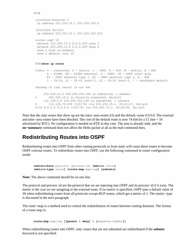
203.250.15.0 255.255.255.252 is subnetted, 1 subnets C 203.250.15.0 is directly connected, Serial0 131.108.0.0 255.255.255.240 is subnetted, 1 subnets O 131.108.79.208 [110/74] via 203.250.15.1, 00:31:27, Serial0 O*IA 0.0.0.0 0.0.0.0 [110/74] via 203.250.15.1, 00:00:00, Serial0

Note that the only routes that show up are the intra−area routes (O) and the default−route 0.0.0.0. The externaland inter−area routes have been blocked. The cost of the default route is now 74 (64 for a T1 line + 10advertised by RTC). No configuration is needed on RTE in this case. The area is already stub, and theno−summary command does not affect the Hello packet at all as the stub command does.

Redistributing Routes into OSPF

Redistributing routes into OSPF from other routing protocols or from static will cause these routes to becomeOSPF external routes. To redistribute routes into OSPF, use the following command in router configurationmode:

redistribute protocol [process−id] [metric value][metric−type value] [route−map map−tag] [subnets]

Note: The above command should be on one line.

The protocol and process−id are the protocol that we are injecting into OSPF and its process−id if it exits. Themetric is the cost we are assigning to the external route. If no metric is specified, OSPF puts a default value of20 when redistributing routes from all protocols except BGP routes, which get a metric of 1. The metric−typeis discussed in the next paragraph.

The route−map is a method used to control the redistribution of routes between routing domains. The formatof a route map is:

route−map map−tag [[permit | deny] | [sequence−number]]

When redistributing routes into OSPF, only routes that are not subnetted are redistributed if the subnetskeyword is not specified.

E1 vs. E2 External Routes

External routes fall under two categories, external type 1 and external type 2. The difference between the twois in the way the cost (metric) of the route is being calculated. The cost of a type 2 route is always the externalcost, irrespective of the interior cost to reach that route. A type 1 cost is the addition of the external cost andthe internal cost used to reach that route. A type 1 route is always preferred over a type 2 route for the samedestination. This is illustrated in the following diagram:

As the above diagram shows, RTA is redistributing two external routes into OSPF. N1 and N2 both have anexternal cost of x. The only difference is that N1 is redistributed into OSPF with a metric−type 1 and N2 isredistributed with a metric−type 2. If we follow the routes as they flow from Area 1 to Area 0, the cost toreach N2 as seen from RTB or RTC will always be x. The internal cost along the way is not considered. Onthe other hand, the cost to reach N1 is incremented by the internal cost. The cost is x+y as seen from RTB andx+y+z as seen from RTC.

If the external routes are both type 2 routes and the external costs to the destination network are equal, thenthe path with the lowest cost to the ASBR is selected as the best path.

Unless otherwise specified, the default external type given to external routes is type 2.

Suppose we added two static routes pointing to E0 on RTC: 16.16.16.0 255.255.255.0 (the /24 notationindicates a 24 bit mask starting from the far left) and 128.213.0.0 255.255.0.0. The following shows thedifferent behaviors when different parameters are used in the redistribute command on RTC:

RTC# interface Ethernet0 ip address 203.250.14.2 255.255.255.0


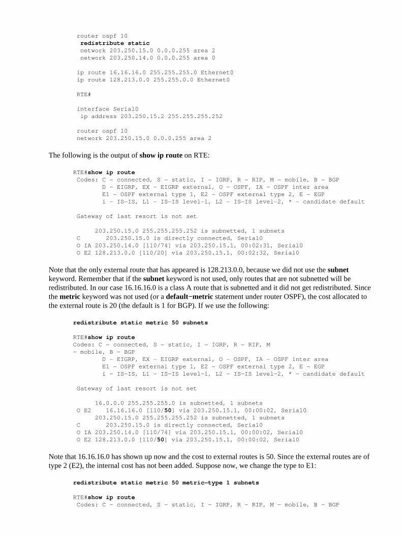
router ospf 10redistribute static

network 203.250.15.0 0.0.0.255 area 2 network 203.250.14.0 0.0.0.255 area 0

ip route 16.16.16.0 255.255.255.0 Ethernet0 ip route 128.213.0.0 255.255.0.0 Ethernet0

RTE#


router ospf 10 network 203.250.15.0 0.0.0.255 area 2

The following is the output of show ip route on RTE:



203.250.15.0 255.255.255.252 is subnetted, 1 subnets C 203.250.15.0 is directly connected, Serial0 O IA 203.250.14.0 [110/74] via 203.250.15.1, 00:02:31, Serial0 O E2 128.213.0.0 [110/20] via 203.250.15.1, 00:02:32, Serial0

Note that the only external route that has appeared is 128.213.0.0, because we did not use the subnetkeyword. Remember that if the subnet keyword is not used, only routes that are not subnetted will beredistributed. In our case 16.16.16.0 is a class A route that is subnetted and it did not get redistributed. Sincethe metric keyword was not used (or a default−metric statement under router OSPF), the cost allocated tothe external route is 20 (the default is 1 for BGP). If we use the following:

redistribute static metric 50 subnets

RTE#show ip routeCodes: C − connected, S − static, I − IGRP, R − RIP, M− mobile, B − BGP D − EIGRP, EX − EIGRP external, O − OSPF, IA − OSPF inter area E1 − OSPF external type 1, E2 − OSPF external type 2, E − EGP i − IS−IS, L1 − IS−IS level−1, L2 − IS−IS level−2, * − candidate default


16.0.0.0 255.255.255.0 is subnetted, 1 subnets O E2 16.16.16.0 [110/50] via 203.250.15.1, 00:00:02, Serial0 203.250.15.0 255.255.255.252 is subnetted, 1 subnets C 203.250.15.0 is directly connected, Serial0 O IA 203.250.14.0 [110/74] via 203.250.15.1, 00:00:02, Serial0 O E2 128.213.0.0 [110/50] via 203.250.15.1, 00:00:02, Serial0

Note that 16.16.16.0 has shown up now and the cost to external routes is 50. Since the external routes are oftype 2 (E2), the internal cost has not been added. Suppose now, we change the type to E1:

redistribute static metric 50 metric−type 1 subnets

RTE#show ip route Codes: C − connected, S − static, I − IGRP, R − RIP, M − mobile, B − BGP

D − EIGRP, EX − EIGRP external, O − OSPF, IA − OSPF inter area E1 − OSPF external type 1, E2 − OSPF external type 2, E − EGP i − IS−IS, L1 − IS−IS level−1, L2 − IS−IS level−2, * − candidate default


16.0.0.0 255.255.255.0 is subnetted, 1 subnets O E1 16.16.16.0 [110/114] via 203.250.15.1, 00:04:20, Serial0 203.250.15.0 255.255.255.252 is subnetted, 1 subnets C 203.250.15.0 is directly connected, Serial0 O IA 203.250.14.0 [110/74] via 203.250.15.1, 00:09:41, Serial0 O E1 128.213.0.0 [110/114] via 203.250.15.1, 00:04:21, Serial0

Note that the type has changed to E1 and the cost has been incremented by the internal cost of S0 which is 64,the total cost is 64+50=114.

Assume that we add a route map to RTC's configuration, we will get the following:



router ospf 10redistribute static metric 50 metric−type 1 subnets route−map STOPUPDATE

network 203.250.15.0 0.0.0.255 area 2 network 203.250.14.0 0.0.0.255 area 0

ip route 16.16.16.0 255.255.255.0 Ethernet0 ip route 128.213.0.0 255.255.0.0 Ethernet0

access−list 1 permit 128.213.0.0 0.0.255.255

route−map STOPUPDATE permit 10 match ip address 1

The route map above will only permit 128.213.0.0 to be redistributed into OSPF and will deny the rest. This iswhy 16.16.16.0 does not show up in RTE's routing table anymore.



203.250.15.0 255.255.255.252 is subnetted, 1 subnets C 203.250.15.0 is directly connected, Serial0 O IA 203.250.14.0 [110/74] via 203.250.15.1, 00:00:04, Serial0 O E1 128.213.0.0 [110/114] via 203.250.15.1, 00:00:05, Serial0

Redistributing OSPF into Other Protocols

Use of a Valid Metric

Whenever you redistribute OSPF into other protocols, you have to respect the rules of those protocols. Inparticular, the metric applied should match the metric used by that protocol. For example, the RIP metric is ahop count ranging between 1 and 16, where 1 indicates that a network is one hop away and 16 indicates that

the network is unreachable. On the other hand IGRP and EIGRP require a metric of the form:

default−metric bandwidth delay reliability loading mtu

VLSM

Another issue to consider is VLSM (Variable Length Subnet Guide)(Appendix C). OSPF can carry multiplesubnet information for the same major net, but other protocols such as RIP and IGRP (EIGRP is OK withVLSM) cannot. If the same major net crosses the boundaries of an OSPF and RIP domain, VLSM informationredistributed into RIP or IGRP will be lost and static routes will have to be configured in the RIP or IGRPdomains. The following example illustrates this problem:

In the above diagram, RTE is running OSPF and RTA is running RIP. RTC is doing the redistributionbetween the two protocols. The problem is that the class C network 203.250.15.0 is variably subnetted, it hastwo different masks 255.255.255.252 and 255.255.255.192. Let us look at the configuration and the routingtables of RTE and RTA:

RTA# interface Ethernet0 ip address 203.250.15.68 255.255.255.192 router rip network 203.250.15.0 RTC# interface Ethernet0 ip address 203.250.15.67 255.255.255.192

interface Serial1 ip address 203.250.15.1 255.255.255.252 router ospf 10 redistribute rip metric 10 subnets network 203.250.15.0 0.0.0.255 area 0 router rip redistribute ospf 10 metric 2 network 203.250.15.0



203.250.15.0 is variably subnetted, 2 subnets, 2 masks

C 203.250.15.0 255.255.255.252 is directly connected, Serial0 O 203.250.15.64 255.255.255.192 [110/74] via 203.250.15.1, 00:15:55, Serial0 RTA#show ip route Codes: C − connected, S − static, I − IGRP, R − RIP, M − mobile, B − BGP D − EIGRP, EX − EIGRP external, O − OSPF, IA − OSPF inter area E1 − OSPF external type 1, E2 − OSPF external type 2, E − EGP i − IS−IS, L1 − IS−IS level−1, L2 − IS−IS level−2, * − candidate default


203.250.15.0 255.255.255.192 is subnetted, 1 subnets C 203.250.15.64 is directly connected, Ethernet0

Note that RTE has recognized that 203.250.15.0 has two subnets while RTA thinks that it has only one subnet(the one configured on the interface). Information about subnet 203.250.15.0 255.255.255.252 is lost in theRIP domain. In order to reach that subnet, a static route needs to be configured on RTA:

RTA# interface Ethernet0 ip address 203.250.15.68 255.255.255.192 router rip network 203.250.15.0

ip route 203.250.15.0 255.255.255.0 203.250.15.67

This way RTA will be able to reach the other subnets.

Mutual Redistribution

Mutual redistribution between protocols should be done very carefully and in a controlled manner. Incorrectconfiguration could lead to potential looping of routing information. A rule of thumb for mutual redistributionis not to allow information learned from a protocol to be injected back into the same protocol. Passiveinterfaces and distribute lists should be applied on the redistributing routers. Filtering information withlink−state protocols such as OSPF is a tricky business. Distribute−list out works on the ASBR to filterredistributed routes into other protocols. Distribute−list in works on any router to prevent routes from beingput in the routing table, but it does not prevent link−state packets from being propagated, downstream routerswould still have the routes. It is better to avoid OSPF filtering as much as possible if filters can be applied onthe other protocols to prevent loops.

To illustrate, suppose RTA, RTC, and RTE are running RIP. RTC and RTA are also running OSPF. BothRTC and RTA are doing redistribution between RIP and OSPF. Let us assume that you do not want the RIPcoming from RTE to be injected into the OSPF domain so you put a passive interface for RIP on E0 of RTC.However, you have allowed the RIP coming from RTA to be injected into OSPF. Here is the outcome:

Note: Do not use the following configuration.

RTE#



router rip network 203.250.15.0



router ospf 10 redistribute rip metric 10 subnets network 203.250.15.0 0.0.0.255 area 0

router rip redistribute ospf 10 metric 2 passive−interface Ethernet0 network 203.250.15.0

RTA#interface Ethernet0 ip address 203.250.15.68 255.255.255.192


router rip redistribute ospf 10 metric 1 network 203.250.15.0

RTC#show ip route Codes: C − connected, S − static, I − IGRP, R − RIP, M − mobile, B − BGP D − EIGRP, EX − EIGRP external, O − OSPF, IA − OSPF inter area E1 − OSPF external type 1, E2 − OSPF external type 2, E − EGP i − IS−IS, L1 − IS−IS level−1, L2 − IS−IS level−2, * − candidate default


203.250.15.0 255.255.255.192 is subnetted, 4 subnets C 203.250.15.0 is directly connected, Serial1 C 203.250.15.64 is directly connected, Ethernet0

R 203.250.15.128 [120/1] via 203.250.15.68, 00:01:08, Ethernet0 [120/1] via 203.250.15.2, 00:00:11, Serial1 O 203.250.15.192 [110/20] via 203.250.15.68, 00:21:41, Ethernet0

Note that RTC has two paths to reach 203.250.15.128 subnet: Serial 1 and Ethernet 0 (E0 is obviously thewrong path). This happened because RTC gave that entry to RTA via OSPF and RTA gave it back via RIPbecause RTA did not learn it via RIP. This example is a very small scale of loops that can occur because of anincorrect configuration. In large networks this situation gets even more aggravated.

In order to fix the situation in our example, you could stop RIP from being sent on RTA's Ethernet 0 via apassive interface. This might not be suitable in case some routers on the Ethernet are RIP only routers. In thiscase, you could allow RTC to send RIP on the Ethernet; this way RTA will not send it back on the wirebecause of split horizon (this might not work on NBMA media if split horizon is off). Split horizon does notallow updates to be sent back on the same interface they were learned from (via the same protocol). Anothergood method is to apply distribute−lists on RTA to deny subnets learned via OSPF from being put back intoRIP on the Ethernet. The latter is the one we will be using:

RTA# interface Ethernet0 ip address 203.250.15.68 255.255.255.192


router rip redistribute ospf 10 metric 1 network 203.250.15.0

distribute−list 1 out ospf 10

And the output of RTC's routing table would be:

RTF#show ip route Codes: C − connected, S − static, I − IGRP, R − RIP, M − mobile, B − BGP D − EIGRP, EX − EIGRP external, O − OSPF, IA − OSPF inter area E1 − OSPF external type 1, E2 − OSPF external type 2, E − EGP i − IS−IS, L1 − IS−IS level−1, L2 − IS−IS level−2, * − candidate default


203.250.15.0 255.255.255.192 is subnetted, 4 subnets C 203.250.15.0 is directly connected, Serial1 C 203.250.15.64 is directly connected, Ethernet0

R 203.250.15.128 [120/1] via 203.250.15.2, 00:00:19, Serial1 O 203.250.15.192 [110/20] via 203.250.15.68, 00:21:41, Ethernet0

Injecting Defaults into OSPF

An autonomous system boundary router (ASBR) can be forced to generate a default route into the OSPFdomain. As discussed earlier, a router becomes an ASBR whenever routes are redistributed into an OSPFdomain. However, an ASBR does not, by default, generate a default route into the OSPF routing domain.

To have OSPF generate a default route use the following:

default−information originate [always] [metric metric−value][metric−type type−value] [route−map map−name]

Note: The above command should be on one line.

There are two ways to generate a default. The first is to advertise 0.0.0.0 inside the domain, but only if theASBR itself already has a default route. The second is to advertise 0.0.0.0 regardless whether the ASBR has adefault route. The latter can be set by adding the keyword always. You should be careful when using thealways keyword. If your router advertises a default (0.0.0.0) inside the domain and does not have a defaultitself or a path to reach the destinations, routing will be broken.

The metric and metric type are the cost and type (E1 or E2) assigned to the default route. The route mapspecifies the set of conditions that need to be satisfied in order for the default to be generated.

Assume that RTE is injecting a default−route 0.0.0.0 into RIP. RTC will have a gateway of last resort of203.250.15.2. RTC will not propagate the default to RTA until we configure RTC with adefault−information originate command.

RTC#show ip route Codes: C − connected, S − static, I − IGRP, R − RIP, M − mobile, B − BGP D − EIGRP, EX − EIGRP external, O − OSPF, IA − OSPF inter area E1 − OSPF external type 1, E2 − OSPF external type 2, E − EGP i − IS−IS, L1 − IS−IS level−1, L2 − IS−IS level−2, * − candidate default


203.250.15.0 255.255.255.192 is subnetted, 4 subnets C 203.250.15.0 is directly connected, Serial1 C 203.250.15.64 is directly connected, Ethernet0 R 203.250.15.128 [120/1] via 203.250.15.2, 00:00:17, Serial1 O 203.250.15.192 [110/20] via 203.250.15.68, 2d23, Ethernet0 R* 0.0.0.0 0.0.0.0 [120/1] via 203.250.15.2, 00:00:17, Serial1 [120/1] via 203.250.15.68, 00:00:32, Ethernet0 RTC#




default−information originate metric 10

router rip redistribute ospf 10 metric 2 passive−interface Ethernet0 network 203.250.15.0

RTA#show ip route



203.250.15.0 255.255.255.192 is subnetted, 4 subnets O 203.250.15.0 [110/74] via 203.250.15.67, 2d23, Ethernet0 C 203.250.15.64 is directly connected, Ethernet0 O E2 203.250.15.128 [110/10] via 203.250.15.67, 2d23, Ethernet0 C 203.250.15.192 is directly connected, Ethernet1

O*E2 0.0.0.0 0.0.0.0 [110/10] via 203.250.15.67, 00:00:17, Ethernet0

Note that RTA has learned 0.0.0.0 as an external route with metric 10. The gateway of last resort is set to203.250.15.67 as expected.

OSPF Design Tips

The OSPF RFC (1583) did not specify any guidelines for the number of routers in an area or number the ofneighbors per segment or what is the best way to architect a network. Different people have differentapproaches to designing OSPF networks. The important thing to remember is that any protocol can fail underpressure. The idea is not to challenge the protocol but rather to work with it in order to get the best behavior.The following are a list of things to consider.

Number of Routers per Area

The maximum number of routers per area depends on several factors, including the following:

What kind of area do you have?• What kind of CPU power do you have in that area?• What kind of media?• Will you be running OSPF in NBMA mode?• Is your NBMA network meshed?• Do you have a lot of external LSAs in the network?• Are other areas well summarized?•

For this reason, it's difficult to specify a maximum number of routers per area. Consult your local sales orsystem engineer for specific network design help.

Number of Neighbors

The number of routers connected to the same LAN is also important. Each LAN has a DR and BDR that buildadjacencies with all other routers. The fewer neighbors that exist on the LAN, the smaller the number ofadjacencies a DR or BDR have to build. That depends on how much power your router has. You could alwayschange the OSPF priority to select your DR. Also if possible, try to avoid having the same router be the DRon more than one segment. If DR selection is based on the highest RID, then one router could accidentlybecome a DR over all segments it is connected to. This router would be doing extra effort while other routersare idle.

Number of Areas per ABR

ABRs will keep a copy of the database for all areas they service. If a router is connected to five areas forexample, it will have to keep a list of five different databases. The number of areas per ABR is a number thatis dependent on many factors, including type of area (normal, stub, NSSA), ABR CPU power, number of

routes per area, and number of external routes per area. For this reason, a specific number of areas per ABRcannot be recommended. Of course, it's better not to overload an ABR when you can always spread the areasover other routers. The following diagram shows the difference between one ABR holding five differentdatabases (including area 0) and two ABRs holding three databases each. Again, these are just guidelines, themore areas you configure per ABR the lower performance you get. In some cases, the lower performance canbe tolerated.

Full Mesh vs. Partial Mesh

Non Broadcast Multi−Access (NBMA) clouds such as Frame Relay or X.25, are always a challenge. Thecombination of low bandwidth and too many link−states is a recipe for problems. A partial mesh topology hasproven to behave much better than a full mesh. A carefully laid out point−to−point or point−to−multipointnetwork works much better than multipoint networks that have to deal with DR issues.

Memory Issues

It is not easy to figure out the memory needed for a particular OSPF configuration. Memory issues usuallycome up when too many external routes are injected in the OSPF domain. A backbone area with 40 routersand a default route to the outside world would have less memory issues compared with a backbone area with 4routers and 33,000 external routes injected into OSPF.

Memory could also be conserved by using a good OSPF design. Summarization at the area border routers anduse of stub areas could further minimize the number of routes exchanged.

The total memory used by OSPF is the sum of the memory used in the routing table ( show ip routesummary ) and the memory used in the link−state database. The following numbers are a rule of thumbestimate. Each entry in the routing table will consume between approximately 200 and 280 bytes plus 44

bytes per extra path. Each LSA will consume a 100 byte overhead plus the size of the actual link stateadvertisement, possibly another 60 to 100 bytes (for router links, this depends on the number of interfaces onthe router). This should be added to memory used by other processes and by the IOS itself. If you really wantto know the exact number, you can do a show memory with and without OSPF being turned on. Thedifference in the processor memory used would be the answer (keep a backup copy of the configs).

Normally, a routing table with less than 500K bytes could be accommodated with 2 to 4 MB RAM; Largenetworks with greater than 500K may need 8 to 16 MB, or 32 to 64 MB if full routes are injected from theInternet.

Summary

The OSPF protocol defined in RFC 1583, provides a high functionality open protocol that allows multiplevendor networks to communicate using the TCP/IP protocol family. Some of the benefits of OSPF are, fastconvergence, VLSM, authentication, hierarchical segmentation, route summarization, and aggregation whichare needed to handle large and complicated networks.

Appendix A: Link−State Database Synchronization

In the above diagram, routers on the same segment go through a series of states before forming a successfuladjacency. The neighbor and DR election are done via the Hello protocol. Whenever a router sees itself in hisneighbor's Hello packet, the state transitions to "2−Way". At that point DR and BDR election is performed onmulti−access segments. A router continues forming an adjacency with a neighbor if either of the two routers isa DR or BDR or they are connected via a point−to−point or virtual link.

In the Exstart state,the two neighbors form a Master/Slave relationship where they agree on a initialsequence number. The sequence number is used to detect old or duplicate Link−State Advertisements (LSA).

In the Exchange state, Database Description Packets (DD) will get exchanged. These are abbreviatedlink−state advertisements in the form of link−state headers. The header supplies enough information toidentify a link. The master node sends DD packets which are acknowledged with DD packets from the slavenode. All adjacencies in exchange state or greater are used by the flooding procedure. These adjacencies arefully capable of transmitting and receiving all types of OSPF routing protocol packets.

In the Loading state, link−state request packets are sent to neighbors, asking for more recent advertisementsthat have been discovered but not yet received. Each router builds a list of required LSAs to bring itsadjacency up to date. A Retransmission List is maintained to make sure that every LSA is acknowledged. Tospecify the number of seconds between link−state advertisement retransmissions for the adjacency you canuse:

ip ospf retransmit−interval seconds

Link−state update packets are sent in response to request packets. The link−state update packets will beflooded over all adjacencies.

In the Full state, the neighbor routers are fully adjacent. The databases for a common area are an exact matchbetween adjacent routers.

Each LSA has an age field that gets periodically incremented while it is contained in the database or as it getsflooded throughout the area. When an LSA reaches a Maxage it gets flushed from the database if that LSA isnot on any neighbors retransmission list.

Link−State Advertisements

Link−state advertisements are broken into five types. Router Links (RL) are generated by all routers. Theselinks describe the state of the router interfaces inside a particular area. These links are only flooded inside therouter's area. Network Links (NL) are generated by a DR of a particular segment; these are an indication ofthe routers connected to that segment. Summary Links (SL) are the inter−area links (type 3); these links willlist the networks inside other areas but still belonging to the autonomous system. Summary links are injectedby the ABR from the backbone into other areas and from other areas into the backbone. These links are usedfor aggregation between areas. Other types of summary links are the asbr−summary links. These are type 4links that point to the ASBR. This is to make sure that all routers know the way to exit the autonomoussystem. The last type is type 5, External Links (EL), these are injected by the ASBR into the domain.

The above diagram illustrates the different link types. RTA generates a router link (RL) into area 1, and it alsogenerates a network link (NL) since it happens the be the DR on that particular segment. RTB is an ABR, andit generates RL into area 1 and area 0. RTB also generates summary links into area 1 and area 0. These linksare the list of networks that are interchanged between the two areas. An ASBR summary link is also injectedby RTB into area 1. This is an indication of the existence of RTD, the autonomous system boundary router(ASBR). Similarly RTC, which is another ABR, generates RL for area 0 and area 2, and a SL (3) into area 2(since it is not announcing any ASBR), and a SL (3,4) into area 0 announcing RTD. RTD generates a RL forarea 2 and generates an EL for external routes learned via BGP. The external routers will be flooded all overthe domain.

The following table is a summary of the link state advertisements.

LSType

Advertisement Description

1Router Link advertisements. Generated by each routerfor each area it belongs to. They describe the states ofthe router's link to the area. These are only floodedwithin a particular area.

2Network Link advertisements. Generated by DesignatedRouters. They describe the set of routers attached to aparticular network. Flooded in the area that contains thenetwork.

3 or 4

Summary Link advertisements. Generated by AreaBorder routers. They describe inter−area (betweenareas) routes. Type 3 describes routes to networks, alsoused for aggregating routes. Type 4 describes routes toASBR.

5AS external link advertisements. Originated by ASBR.They describe routes to destinations external to the AS.Flooded all over except stub areas.

If you look at the OSPF database in detail, using show ip ospf database detail , you will see differentkeywords such as Link−Data, Link−ID, and Link−state ID. These terms become confusing as the value ofeach depends on the link state type and the link−type. We will go over this terminology and will provide adetailed example on the OSPF database as seen from the router.

The Link−State ID basically defines the identity of the link−state depending on the LS type. Router Links areidentified by the router ID (RID) of the router that originated the advertisement. Network Links are identifiedby the relative IP address of the DR. This makes sense because Network Links are originated by theDesignated Router. Summary Links (type 3) are identified by the IP network numbers of the destinationsthey are pointing at. ASBR Summary Links (Summary Links type 4) are identified by the RID of the ASBR.Finally, External Links are identified by the IP network numbers of the external destinations they arepointing at. The following table summarizes this information:

LSType Link State ID (In the high level view of the database

when referencing a router this is called Link ID)1

The originating Router's Router ID (RID).2 The IP interface address of the network's Designated

Router.

3The destination network number.

4The router ID of the described AS boundary router.

5The external network number.

Next, we will describe the different links available:

Stub network links: This term has nothing to do with stub areas. A stub segment is a segment that has onerouter only attached to it. An Ethernet or Token Ring segment that has one attached router is considered a linkto a stub network. A loopback interface is also considered a link to stub network with a 255.255.255.255 mask(Host route).

Point−to−point links: These could be physical or logical (subinterfaces) point−to−point serial linkconnections. These links could be numbered (an IP address is configured on the link) or unnumbered.

Transit links: These are interfaces connected to networks that have more than one router attached, hence thename transit.

Virtual links: These are logical links that connect areas that do not have physical connections to thebackbone. Virtual links are treated as numbered point−to−point links.

The link−ID is an identification of the link itself. This is different for each link type. A transit link isidentified by the IP address of the DR on that link. A numbered point−to−point link is identified by the RIDof the neighbor router on the point−to−point link. Virtual links are identical to point−to−point links.

Finally, links to stub networks are identified by the IP address of the interface to the stub network. Thefollowing table summarizes this information:

Link Type Link ID (This applies toindividual Links)

Point−to−PointNeighbor Router ID

Link to transit networkInterface address of DR

Link to stub network (In case ofloopback mask is 255.255.255.255)

Network/subnet numberVirtual Link

Neighbor Router ID

The Link Data is the IP address of the link, except for stub network where the link data is the network mask.

Link TypeLink Data

Stub networkNetwork Mask

Other networks (applies to routerlinks only) Router's associated IP

interface address

Finally, an Advertising Router is the RID of the router that has sent the LSA.

OSPF Database Example

Given the network diagram above, the following configurations, and the IP route tables, let us look at differentways of understanding the OSPF database.

RTA# interface Loopback0 ip address 203.250.13.41 255.255.255.255



router ospf 10 network 203.250.0.0 0.0.255.255 area 0

RTA#show ip route Codes: C − connected, S − static, I − IGRP, R − RIP, M − mobile, B − BGP D − EIGRP, EX − EIGRP external, O − OSPF, IA − OSPF inter area E1 − OSPF external type 1, E2 − OSPF external type 2, E − EGP

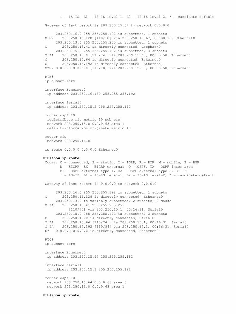
i − IS−IS, L1 − IS−IS level−1, L2 − IS−IS level−2, * − candidate default


203.250.16.0 255.255.255.192 is subnetted, 1 subnets O E2 203.250.16.128 [110/10] via 203.250.15.67, 00:00:50, Ethernet0 203.250.13.0 255.255.255.255 is subnetted, 1 subnets C 203.250.13.41 is directly connected, Loopback0 203.250.15.0 255.255.255.192 is subnetted, 3 subnets O IA 203.250.15.0 [110/74] via 203.250.15.67, 00:00:50, Ethernet0 C 203.250.15.64 is directly connected, Ethernet0 C 203.250.15.192 is directly connected, Ethernet1 O*E2 0.0.0.0 0.0.0.0 [110/10] via 203.250.15.67, 00:00:50, Ethernet0

RTE# ip subnet−zero



router ospf 10 redistribute rip metric 10 subnets network 203.250.15.0 0.0.0.63 area 1 default−information originate metric 10

router rip network 203.250.16.0

ip route 0.0.0.0 0.0.0.0 Ethernet0



203.250.16.0 255.255.255.192 is subnetted, 1 subnets C 203.250.16.128 is directly connected, Ethernet0 203.250.13.0 is variably subnetted, 2 subnets, 2 masks O IA 203.250.13.41 255.255.255.255 [110/75] via 203.250.15.1, 00:16:31, Serial0 203.250.15.0 255.255.255.192 is subnetted, 3 subnets C 203.250.15.0 is directly connected, Serial0 O IA 203.250.15.64 [110/74] via 203.250.15.1, 00:16:31, Serial0 O IA 203.250.15.192 [110/84] via 203.250.15.1, 00:16:31, Serial0 S* 0.0.0.0 0.0.0.0 is directly connected, Ethernet0

RTC# ip subnet−zero



router ospf 10 network 203.250.15.64 0.0.0.63 area 0 network 203.250.15.0 0.0.0.63 area 1

RTF#show ip route



203.250.16.0 255.255.255.192 is subnetted, 1 subnets O E2 203.250.16.128 [110/10] via 203.250.15.2, 04:49:05, Serial1 203.250.13.0 255.255.255.255 is subnetted, 1 subnets O 203.250.13.41 [110/11] via 203.250.15.68, 04:49:06, Ethernet0 203.250.15.0 255.255.255.192 is subnetted, 3 subnets C 203.250.15.0 is directly connected, Serial1 C 203.250.15.64 is directly connected, Ethernet0 O 203.250.15.192 [110/20] via 203.250.15.68, 04:49:06, Ethernet0 O*E2 0.0.0.0 0.0.0.0 [110/10] via 203.250.15.2, 04:49:06, Serial1

General View of the Database

RTC#show ip ospf database

OSPF Router with ID (203.250.15.67) (Process ID 10)

Router Link States (Area 1)

Link ID ADV Router Age Seq# Checksum Link count203.250.15.67 203.250.15.67 48 0x80000008 0xB112 2203.250.16.130 203.250.16.130 212 0x80000006 0x3F44 2

Summary Net Link States (Area 1)

Link ID ADV Router Age Seq# Checksum203.250.13.41 203.250.15.67 602 0x80000002 0x90AA203.250.15.64 203.250.15.67 620 0x800000E9 0x3E3C203.250.15.192 203.250.15.67 638 0x800000E5 0xA54E


Link ID ADV Router Age Seq# Checksum Link count203.250.13.41 203.250.13.41 179 0x80000029 0x9ADA 3203.250.15.67 203.250.15.67 675 0x800001E2 0xDD23 1

Net Link States (Area 0)

Link ID ADV Router Age Seq# Checksum203.250.15.68 203.250.13.41 334 0x80000001 0xB6B5


Link ID ADV Router Age Seq# Checksum203.250.15.0 203.250.15.67 792 0x80000002 0xAEBD

Summary ASB Link States (Area 0)

Link ID ADV Router Age Seq# Checksum203.250.16.130 203.250.15.67 579 0x80000001 0xF9AF

AS External Link States

Link ID ADV Router Age Seq# Checksum Tag0.0.0.0 203.250.16.130 1787 0x80000001 0x98CE 10203.250.16.128 203.250.16.130 5 0x80000002 0x93C4 0

This is a general look at the whole OSPF database. The database is listed according to the areas. In this case,we are looking at RTC's database which is an ABR. Both area 1 and area 0's databases are listed. Area 1 is

composed of router links and summary links. No network links exist because no DR exists on any of thesegments in area 1. No Summary ASBR links exist in area 1 because the only ASBR happens to be in area 0.External links do not belong to any particular area as they are flooded all over. Note that all the links are thecumulative links collected from all routers in an area.

We will mainly concentrate on the database in area 0. The Link−ID indicated here is actually the Link−StateID. This is a representation of the whole router, not a particular link. This is a bit confusing, but just rememberthat this high level Link−ID (should be Link−State ID) represents the whole router and not just a link.

Router Links


Link ID ADV Router Age Seq# Checksum Link count 203.250.13.41 203.250.13.41 179 0x80000029 0x9ADA 3 203.250.15.67 203.250.15.67 675 0x800001E2 0xDD23 1

We will start with the router links. There are two entries listed for 203.250.13.41 and 203.250.15.67, these arethe RIDs of the two routers in area 0. The number of links in area 0 for each router is also indicated. RTA hasthree links to area 0 and RTC has one link. A detailed view of RTC's router links follows:

RTC#show ip ospf database router 203.250.15.67



LS age: 1169 Options: (No TOS−capability) LS Type: Router Links Link State ID: 203.250.15.67 Advertising Router: 203.250.15.67 LS Seq Number: 80000008 Checksum: 0xB112 Length: 48 Area Border Router Number of Links: 2

Link connected to: another Router (point−to−point) (Link ID) Neighboring Router ID: 203.250.16.130 (Link Data) Router Interface address: 203.250.15.1 Number of TOS metrics: 0 TOS 0 Metrics: 64

Link connected to: a Stub Network (Link ID) Network/subnet number: 203.250.15.0 (Link Data) Network Mask: 255.255.255.192 Number of TOS metrics: 0 TOS 0 Metrics: 64

One thing to note here is that OSPF generates an extra stub link for each point−to−point interface. Do not getconfused if you see the link count larger than the number of physical interfaces.


LS age: 1227 Options: (No TOS−capability)

LS Type: Router Links Link State ID: 203.250.15.67 Advertising Router: 203.250.15.67 LS Seq Number: 80000003 Checksum: 0xA041

Length: 36 Area Border Router

Number of Links: 1

Link connected to: a Transit Network (Link ID) Designated Router address: 203.250.15.68 (Link Data) Router Interface address: 203.250.15.67 Number of TOS metrics: 0 TOS 0 Metrics: 10

Note that the Link ID is equal to the IP address (not the RID) of the attached DR; in this case it is203.250.15.68. The Link Data is RTC's own IP address.

Network Links


Link ID ADV Router Age Seq# Checksum203.250.15.68 203.250.13.41 334 0x80000001 0xB6B5

One network link is listed, indicated by the interface IP address (not the RID) of the DR, in this case203.250.15.68. A detailed view of this entry follows:

RTC#show ip ospf database network



Routing Bit Set on this LSA LS age: 1549 Options: (No TOS−capability) LS Type: Network Links

Link State ID: 203.250.15.68 (address of Designated Router) Advertising Router: 203.250.13.41 LS Seq Number: 80000002 Checksum: 0xB4B6 Length: 32 Network Mask: 255.255.255.192

Attached Router: 203.250.13.41 Attached Router: 203.250.15.67

Note that the network link lists the RIDs of the routers attached to the transit network; in this case the RIDs ofRTA and RTC are listed.

Summary Links


Link ID ADV Router Age Seq# Checksum203.250.15.0 203.250.15.67 792 0x80000002 0xAEBDArea 0 has one summary link represented by the IP network address of thelink 203.250.15.0. This link was injected by the ABR RTC from area 1 intoarea 0. A detailed view of this summary link follows, summary links forarea 1 are not listed here:

RTC#show ip ospf database summary (area 1 is not listed)



LS Type: Summary Links(Network)Link State ID: 203.250.15.0 (summary Network Number)

Advertising Router: 203.250.15.67 LS Seq Number: 80000003 Checksum: 0xACBE Length: 28 Network Mask: 255.255.255.192 TOS: 0 Metric: 64

Summary ASBR Links


Link ID ADV Router Age Seq# Checksum203.250.16.130 203.250.15.67 579 0x80000001 0xF9AF

This is an indication of who the ASBR is. In this case the ASBR is RTE represented by its RID203.250.16.130. The advertising router for this entry into area 0 is RTC with RID 203.250.15.67. A detailedview of the summary ASBR entry follows:

RTC#show ip ospf database asbr−summary




LS Type: Summary Links(AS Boundary Router) Link State ID: 203.250.16.130 (AS Boundary Router address) Advertising Router: 203.250.15.67 LS Seq Number: 80000003 Checksum: 0xF5B1 Length: 28 Network Mask: 0.0.0.0 TOS: 0 Metric: 64

External Links


Link ID ADV Router Age Seq# Checksum Tag0.0.0.0 203.250.16.130 1787 0x80000001 0x98CE 10203.250.16.128 203.250.16.130 5 0x80000002 0x93C4 0

We have two external Links, the first one is the 0.0.0.0 injected into OSPF via the default−informationoriginate command. The other entry is network 203.250.16.12 8 which is injected into OSPF byredistribution. The router advertising these networks is 203.250.16.130, the RID of RTE. The following is thedetailed view of the external routes:

RTC#show ip ospf database external



Routing Bit Set on this LSA LS age: 208 Options: (No TOS−capability)

LS Type: AS External Link Link State ID: 0.0.0.0 (External Network Number ) Advertising Router: 203.250.16.130 LS Seq Number: 80000002 Checksum: 0x96CF Length: 36

Network Mask: 0.0.0.0 Metric Type: 2 (Larger than any link state path) TOS: 0 Metric: 10

Forward Address: 0.0.0.0 External Route Tag: 10

Routing Bit Set on this LSA LS age: 226 Options: (No TOS−capability)

LS Type: AS External Link Link State ID: 203.250.16.128 (External Network Number) Advertising Router: 203.250.16.130 LS Seq Number: 80000002 Checksum: 0x93C4 Length: 36 Network Mask: 255.255.255.192 Metric Type: 2 (Larger than any link state path) TOS: 0 Metric: 10

Forward Address: 0.0.0.0 External Route Tag: 0

Note the forward address. Whenever this address is 0.0.0.0 it indicates that the external routes are reachablevia the advertising router, in this case 203. 250.16.130. This is why the identity of the ASBR is injected byABRs into other areas using ASBR summary links.

This forward address is not always 0.0.0.0. In some cases, it could be the IP address of another router on thesame segment. The following diagram will illustrate this situation:

In the above situation RTB, is running BGP with RTA, and OSPF with the rest of the domain. RTA is notrunning OSPF. RTB is redistributing BGP routes into OSPF. According to OSPF, RTB is an ASBRadvertising external routes. The forwarding address in this case is set to 125.211.1.1 and not to the advertisingrouter (0.0.0.0) RT B. This makes sense because there is no need to make the extra hop. An important thing toremember is that routers inside the OSPF domain should be able to reach the forwarding address via OSPF inorder for the external routes to be put in the IP routing table. If the forwarding address is reached via someother protocol or no t accessible, the external entries would be in the database but not in the IP routing table.

Another situation would arise if both RTB and RTC are ASBRs (RTC is also running BGP with RTA). In thissituation, in order to eliminate the duplication of the effort, one of the two routers will not advertise (willflush) the external routes. T he router with the higher RID will win.

The Full Database

Finally, this is a listing of the whole database as an exercise. You should now b e able to go over each entryand explain what is going on:

RTC#show ip ospf database router



LS age: 926 Options: (No TOS−capability) LS Type: Router Links Link State ID: 203.250.15.67 Advertising Router: 203.250.15.67 LS Seq Number: 80000035 Checksum: 0x573F Length: 48 Area Border Router Number of Links: 2 Link connected to: another Router (point−to−point) (Link ID) Neighboring Router ID: 203.250.16.130 (Link Data) Router Interface address: 203.250.15.1 Number of TOS metrics: 0 TOS 0 Metrics: 64


Routing Bit Set on this LSA LS age: 958 Options: (No TOS−capability) LS Type: Router Links Link State ID: 203.250.16.130 Advertising Router: 203.250.16.130 LS Seq Number: 80000038 Checksum: 0xDA76 Length: 48 AS Boundary Router Number of Links: 2

Link connected to: another Router (point−to−point) (Link ID) Neighboring Router ID: 203.250.15.67 (Link Data) Router Interface address: 203.250.15.2 Number of TOS metrics: 0 TOS 0 Metrics: 64



Routing Bit Set on this LSA LS age: 1107 Options: (No TOS−capability) LS Type: Router Links Link State ID: 203.250.13.41 Advertising Router: 203.250.13.41 LS Seq Number: 8000002A Checksum: 0xC0B0 Length: 60 AS Boundary Router Number of Links: 3

Link connected to: a Stub Network

(Link ID) Network/subnet number: 203.250.13.41 (Link Data) Network Mask: 255.255.255.255 Number of TOS metrics: 0 TOS 0 Metrics: 1



LS age: 1575 Options: (No TOS−capability) LS Type: Router Links Link State ID: 203.250.15.67 Advertising Router: 203.250.15.67 LS Seq Number: 80000028 Checksum: 0x5666 Length: 36 Area Border Router Number of Links: 1


RTC#show ip ospf database network



Routing Bit Set on this LSA LS age: 1725 Options: (No TOS−capability) LS Type: Network Links Link State ID: 203.250.15.68 (address of Designated Router) Advertising Router: 203.250.13.41 LS Seq Number: 80000026 Checksum: 0x6CDA Length: 32 Network Mask: 255.255.255.192 Attached Router: 203.250.13.41 Attached Router: 203.250.15.67

RTC#show ip ospf database summary



LS age: 8 Options: (No TOS−capability) LS Type: Summary Links(Network) Link State ID: 203.250.13.41 (summary Network Number) Advertising Router: 203.250.15.67 LS Seq Number: 80000029 Checksum: 0x42D1

Length: 28 Network Mask: 255.255.255.255 TOS: 0 Metric: 11

LS age: 26 Options: (No TOS−capability) LS Type: Summary Links(Network) Link State ID: 203.250.15.64 (summary Network Number) Advertising Router: 203.250.15.67 LS Seq Number: 80000030 Checksum: 0xB182 Length: 28 Network Mask: 255.255.255.192 TOS: 0 Metric: 10

LS age: 47 Options: (No TOS−capability) LS Type: Summary Links(Network) Link State ID: 203.250.15.192 (summary Network Number) Advertising Router: 203.250.15.67 LS Seq Number: 80000029 Checksum: 0x1F91 Length: 28 Network Mask: 255.255.255.192 TOS: 0 Metric: 20


LS age: 66 Options: (No TOS−capability) LS Type: Summary Links(Network) Link State ID: 203.250.15.0 (summary Network Number) Advertising Router: 203.250.15.67 LS Seq Number: 80000025 Checksum: 0x68E0 Length: 28 Network Mask: 255.255.255.192 TOS: 0 Metric: 64

RTC#show ip ospf asbr−summary



LS age: 576 Options: (No TOS−capability) LS Type: Summary Links(AS Boundary Router) Link State ID: 203.250.16.130 (AS Boundary Router address) Advertising Router: 203.250.15.67 LS Seq Number: 80000024 Checksum: 0xB3D2 Length: 28 Network Mask: 0.0.0.0 TOS: 0 Metric: 64

RTC#show ip ospf database external



Routing Bit Set on this LSA LS age: 305 Options: (No TOS−capability) LS Type: AS External Link Link State ID: 0.0.0.0 (External Network Number) Advertising Router: 203.250.16.130 LS Seq Number: 80000001 Checksum: 0x98CE

Length: 36 Network Mask: 0.0.0.0 Metric Type: 2 (Larger than any link state path) TOS: 0 Metric: 10 Forward Address: 0.0.0.0 External Route Tag: 10

Routing Bit Set on this LSA LS age: 653 Options: (No TOS−capability) LS Type: AS External Link Link State ID: 203.250.16.128 (External Network Number) Advertising Router: 203.250.16.130 LS Seq Number: 80000024 Checksum: 0x4FE6 Length: 36 Network Mask: 255.255.255.192 Metric Type: 2 (Larger than any link state path) TOS: 0 Metric: 10 Forward Address: 0.0.0.0 External Route Tag: 0

Appendix B: OSPF and IP Multicast Addressing

OSPF used IP multicast to exchange Hello packets and Link State Updates. An IP multicast address isimplemented using class D addresses. A class D address ranges from 224.0.0.0 to 239.255.255.255.

Some special IP multicast addresses are reserved for OSPF:

224.0.0.5: All OSPF routers should be able to transmit and listen to this address.• 224.0.0.6: All DR and BDR routers should be able to transmit and listen to this address.•

The mapping between IP multicast addresses and MAC addresses has the following rule:

For multiaccess networks that support multicast, the low order 23 bits of the IP address are used as the loworder bits of the MAC multicast address 01−005E−00−00− 00. For example:

224.0.0.5 would be mapped to 01−00−5E−00−00−05• 224.0.0.6 would be mapped to 01−00−5E−00−00−06•

OSPF uses broadcast on Token Ring networks.

Appendix C: Variable Length Subnet Masks (VLSM)

The following is a binary/decimal conversion chart:

0000 0001 0010 0011 0100 0101 0110 0111

00000 16 0000 32 0000 48 0000 64 0000 80 0000 96 0000 112 0000

10001 17 0001 33 0001 49 0001 65 0001 81 0001 97 0001 113 0001

20010 18 0010 34 0010 50 0010 66 0010 82 0010 98 0010 114 0010

30011 19 0011 35 0011 51 0011 67 0011 83 0011 99 0011 115 0011

40100 20 0100 36 0100 52 0100 68 0100 84 0100 100 0100 116 0100

50101 21 0101 37 0101 53 0101 69 0101 85 0101 101 0101 117 0101

60110 22 0110 38 0110 54 0110 70 0110 86 0110 102 0110 118 0110

70111 23 0111 39 0111 55 0111 71 0111 87 0111 103 0111 119 0111

81000 24 1000 40 1000 56 1000 72 1000 88 1000 104 1000 120 1000

91001 25 1001 41 1001 57 1001 73 1001 89 1001 105 1001 121 1001

101010 26 1010 42 1010 58 1010 74 1010 90 1010 106 1010 122 1010

111011 27 1011 43 1011 59 1011 75 1011 91 1011 107 1011 123 1011

121100 28 1100 44 1100 60 1100 76 1100 92 1100 108 1100 124 1100

131101 29 1101 45 1101 61 1101 77 1101 93 1101 109 1101 125 1101

141110 30 1110 46 1110 62 1110 78 1110 94 1110 110 1110 126 1110

151111 31 1111 47 1111 63 1111 79 1111 95 1111 111 1111 127 1111

1000 1001 1010 1011 1100 1101 1110 1111128

0000 144 0000 160 0000 176 0000 192 0000 208 0000 224 0000 240 0000129

0001 145 0001 161 0001 177 0001 193 0001 209 0001 225 0001 241 0001130

0010 146 0010 162 0010 178 0010 194 0010 210 0010 226 0010 242 0010131

0011 147 0011 163 0011 179 0011 195 0011 211 0011 227 0011 243 0011132

0100 148 0100 164 0100 180 0100 196 0100 212 0100 228 0100 244 0100133

0101 149 0101 165 0101 181 0101 197 0101 213 0101 229 0101 245 0101134

0110 150 0110 166 0110 182 0110 198 0110 214 0110 230 0110 246 0110135

0111 151 0111 167 0111 183 0111 199 0111 215 0111 231 0111 247 0111136

1000 152 1000 168 1000 184 1000 200 1000 216 1000 232 1000 248 1000137

1001 153 1001 169 1001 185 1001 201 1001 217 1001 233 1001 249 1001138

1010 154 1010 170 1010 186 1010 202 1010 218 1010 234 1010 250 1010139

1011 155 1011 171 1011 187 1011 203 1011 219 1011 235 1011 251 1011140

1100 156 1100 172 1100 188 1100 204 1100 220 1100 236 1100 252 1100141

1101 157 1101 173 1101 189 1101 205 1101 221 1101 237 1101 253 1101142

1110 158 1110 174 1110 190 1110 206 1110 222 1110 238 1110 254 1110143

1111 159 1111 175 1111 191 1111 207 1111 223 1111 239 1111 255 1111

The idea behind variable length subnet masks is to offer more flexibility in dealing with dividing a major netinto multiple subnets and still being able to maintain an adequate number of hosts in each subnet. WithoutVLSM one subnet mask only can be applied to a major network. This restricts the number of hosts given thenumber of subnets required. If you pick the mask such that you have enough subnets, you are not able to

allocate enough hosts in each subnet. The same is true for the hosts; a mask that allows enough hosts mightnot provide enough subnet space.

For example, suppose you were assigned a class C network 192.214.11.0 and you need to divide that networkinto three subnets with 100 hosts in one subnet and 50 hosts for each of the remaining subnets. Ignore the twoend limits 0 and 255, and you have theoretically available to you 256 addresses (192.214.11.0 −192.214.11.255). This cannot be done without VLSM.

There are a handful of subnet masks that can be used; note that a mask should have a contiguous number ofones that start from the left and the rest of the bits are all 0s.

−252 (1111 1100) The address space is divided into 64. −248 (1111 1000) The address space is divided into 32. −240 (1111 0000) The address space is divided into 16. −224 (1110 0000) The address space is divided into 8. −192 (1100 0000) The address space is divided into 4. −128 (1000 0000) The address space is divided into 2.

Without VLSM you have the choice to use mask 255.255.255.128 and divide the addresses into 2 subnetswith 128 hosts each or use 255.255.255.192 and divide the space into 4 subnets with 64 hosts each. This doesnot meet the requirement. If you use multiple masks, you can use mask 128 and further subnet the secondchunk of addresses with mask 192. This table shows how you have divided the address space accordingly.

Now, be careful in allocating the IP addresses to each mask. Once you assign an IP address to the router or toa host, you have used up the whole subnet for that segment. For example, if you assign 192.214.11.10255.255.255.128 to E2, the whole range of addresses between 192.214.11.0 and 192.214.11.127 is consumedby E2. In the same way if you assign 192.214.11.160 255.255.255.128 to E2, the whole range of addressesbetween 192.214.11.128 and 192.214.11.255 is consumed by the E2 segment.

This is an illustration of how the router interprets these addresses. Remember that any time you use a maskdifferent than the natural mask, for instance if you are subnetting, the router complains if the combination IPaddress and mask result in a subnet zero. Use the ip subnet−zero command on the router in order to resolvethis issue.

RTA# ip subnet−zero interface Ethernet2 ip address 192.214.11.10 255.255.255.128

interface Ethernet3 ip address 192.214.11.160 255.255.255.192 interface Ethernet4 ip address 192.214.11.226 255.255.255.192

RTA#show ip route connected 192.214.11.0 is variably subnetted, 3 subnets, 2 masks C 192.214.11.0 255.255.255.128 is directly connected, Ethernet2 C 192.214.11.128 255.255.255.192 is directly connected, Ethernet3 C 192.214.11.192 255.255.255.192 is directly connected, Ethernet4

Related Information

OSPF and MTU• OSPF neighbors are stuck in exstart and exchange state due to MTU mismatch• OSPF Support Page• OSPF: Frequently Asked Questions• Technical Support & Documentation − Cisco Systems•

Contacts & Feedback | Help | Site Map© 2012 − 2013 Cisco Systems, Inc. All rights reserved. Terms & Conditions | Privacy Statement | Cookie Policy | Trademarks ofCisco Systems, Inc.

Updated: Aug 10, 2005 Document ID: 7039

Documents

Cisco - OSPF Design Guidefaculty.weber.edu/kcuddeback/Common_Items/OSPF Configuration.pdf · OSPF and Route Summarization Inter−Area Route Summarization External Route Summarization