Embed Size (px)
Citation preview

Fakultat fur Informatik und Automatisierung
Multi-Dimensional Signal Decomposition
Techniques for the Analysis of EEG Data
Dipl.-Ing. Martin Weis,geboren am 13.05.1983, Suhl, Deutschland
Dissertation zur Erlangung desakademischen Grades Doktor-Ingenieur (Dr.-Ing.)
Anfertigung im: Fachgebiet Biosignalverarbeitung
Institut fur Biomedizinische Technik
Gutachter: Prof. Dr.-Ing. habil. Peter Husar
Prof. Dr.-Ing. Giovanni Del Galdo
Prof. Dr.-Ing. Joao Paulo Carvalho Lustosa da Costa
Vorgelegt am: 27.08.2014
Verteidigt am: 19.02.2015
urn:nbn:de:gbv:ilm1-2015000127


iii
Acknowledgements
Many researchers and colleagues from the Communication Research Lab and the Biosignal
Processing Group at the Technische Universitat Ilmenau influenced the development of this
thesis, and therefore deserve my sincere gratitude.
First of all i would like to thank my supervisor Univ.-Prof. Dr.-Ing. habil. Peter Husar for
giving me the opportunity to work on this thesis. His continuous support and encouragement
to transfer the theoretical results on tensor decompositions to biomedical applications renewed
my motivation for this area of research.
I also want to express my gratitude to Univ.-Prof. Dr.-Ing. Martin Haardt, who directed me to
the field of multi-linear algebra and array signal processing. In the time i worked in his lab i
learned most of what i know about scientific principles, and how to present scientific research
in an exact and comprehensive manner.
Furthermore, i want to thank Professor Adjunto Dr.-Ing. Joao Paulo Carvalho Lustosa da Costa
and Univ.-Prof. Dr.-Ing. Giovanni Del Galdo for reviewing this thesis and for their valuable
comments in the final stages of this work.
Finally, i want to thank all my colleagues from the Biosignal Processing Group and the Com-
munication Research Lab for their support and fruitful discussions. Explicitly, i want to thank
M. Sc. Judith Mengelkamp for reading this thesis. My biggest gratitude deserves Dr.-Ing. Flo-
rian Romer, one of the most ingenious persons i ever learned know. His efficiency in solving
scientific problems and his extensive knowledge was always an inspiring example for me. The
successful long term collaboration with him greatly influenced the content of this work.


v
Abstract
In this thesis, we investigate multi-dimensional blind signal decomposition techniques for the
processing of the ElectroEncephaloGram (EEG). Thereby, it is the objective to separate the
scalp projections of the underlying neural sources in order to enable a topographic analysis of
the spatial distribution of each source. This major objective of EEG signal processing can be
used in order to analyze and to diagnose neural diseases such as epilepsy.
The multi-dimensional EEG signal decomposition techniques involve complex computational
methods, such as tensor decompositions and Time-Frequency Analysis (TFA). For the ten-
sor decompositions, we investigate the PARAllel FACtor (PARAFAC) analysis as well as the
PARAFAC2 analysis. For both tensor decompositions we develop a robust normalization pro-
cedure, which reduces their inherent ambiguities to a minimum. This enables to select the best
model parameters among different PARAFAC / PARAFAC2 estimates. The normalization also
allows to evaluate the influence of the extracted multi-dimensional components. Furthermore,
we present a computational method for the PARAFAC decomposition of dual-symmetric tensors
using Procrustes estimation and Khatri-Rao factorization (ProKRaft). Thereby, ProKRaft out-
performs current state-of-the-art algorithms. By exploiting the connection between PARAFAC
and the Independent Component Analysis (ICA), we also derive a ProKRaft based ICA algo-
rithm.
For the TFA of EEG data, we investigate the performance of various methods, such as the Short
Time Fourier Transform (STFT), different Wavelet transformations, and Wigner-Ville based
techniques. Thereby, we suggest the use of the Smoothed Pseudo Wigner-Ville Distribution
(SPWVD) or the Reduced Interference Distribution (RID) for the processing of EEG with a
special respect to the subsequent tensor decomposition. Our simulations show that only the
SPWVD and the RID provide a sufficient time-frequency resolution while maintaining efficient
cross-term suppression.
For the separation of EEG sources signals, we introduce the PARAFAC2 based EEG decompo-
sition strategy. In contrast to other methods, this technique allows to identify dynamic EEG
sources which exhibit a time-varying spatial activation. Furthermore, it is possible to extract the
exact temporal evolution of these spatial patterns. The advantages of this method are verified
based on synthetic EEG and with the help of measured Visual Evoked Potentials (VEP).


vii
Zusammenfassung
Im Rahmen dieser Dissertation werden mehrdimensionale blinde Signalzerlegungsmethoden fur
die Verarbeitung des Elektroenzephalogramms (EEG) untersucht. Dabei ist es das wesentliche
Ziel, die Projektionen der zu Grunde liegenden neuronalen Quellen zu extrahieren, um eine
topographische Analyse jeder einzelnen Quelle zu ermoglichen. Dies ist eine der Hauptaufgaben
der EEG Signalverarbeitung, die die Analyse und Diagnose neuronaler Pathologien, wie z.B.
Epilepsie, ermoglichen soll.
Die mehrdimensionalen EEG Signalzerlegungsmethoden beinhalten komplexe Rechenmethoden,
wie die Tensor Zerlegung und die Zeit-Frequenz Analyse. Fur die Tensor Zerlegung wird in
dieser Arbeit die PARAllel FACtor (PARAFAC) Analyse, sowie die PARAFAC2 Analyse un-
tersucht. Fur diese beiden Tensor Zerlegungen wird eine robuste Normalisierung vorgestellt,
die die vorhandenen Mehrdeutigkeiten in den Zerlegungsmodellen auf ein Minimum reduziert.
Dies ermoglicht die Auswahl der besten Modellparameter aus einer Vielzahl unterschiedlicher
PARAFAC / PARAFAC2 Schatzungen. Diese Normalisierung erlaubt es auch, den Einfluss
der extrahierten mehrdimensionalen Komponenten zu beurteilen. Des Weiteren wird ein Algo-
rithmus zur Berechnung der PARAFAC Zerlegung dual-symmetrischer Tensoren auf Basis der
Procrustes estimation and Khatri-Rao factorization (ProKRaft) vorgestellt. Der ProKRaft Algo-
rithmus erreicht dabei eine bessere Performance gegenuber vergleichbaren Algorithmen aus der
Literatur. Durch Ausnutzung der Beziehung zwischen PARAFAC und der Independent Compo-
nent Analysis (ICA), wird zusatzlich ein ProKRaft basierter ICA Algorithmus hergeleitet und
analysiert.
Fur die Zeit-Frequenz Analyse von EEG Daten werden in dieser Arbeit zahlreiche Methoden, wie
z.B. die Short Time Fourier Transform (STFT), verschiedene Wavelet Transformationen, sowie
verschiedene Wigner-Ville basierte Methoden, untersucht. Als Ergebnis dieser Untersuchungen,
auch im Hinblick auf die folgende Tensor Zerlegung, wird die Verwendung der Smoothed Pseudo
Wigner-Ville Distribution (SPWVD) oder der Reduced Interference Distribution (RID) vorge-
schlagen. Der Grund hierfur ist in der hinreichend guten Zeit-Frequenz Auflosung dieser beiden
Verfahren zu finden. Dabei ermoglichen beide Methoden gleichzeitig eine effektive Kreuzterm-
unterdruckung.

viii Zusammenfassung
Zur Trennung von EEG Quellsignalen, fuhren wir eine PARAFAC2 basierte Zerlegungsstrategie
ein. Im Vergleich zu anderen Methoden aus der Literatur, erlaubt diese Zerlegungsstrategie die
Extraktion von dynamischen EEG Quellen, die eine zeitvariante raumliche Verteilung aufweisen.
Die exakte zeitliche Lokalisierung dieser raumlichen Verteilungen ist moglich. Die Vorteile die-
ser Zerlegungsmethode werden anhand von synthetischen EEG Daten, und anhand gemessener
Visuell Evozierter Potentiale (VEP) nachgewiesen.

Contents ix
Contents
Acknowledgements iii
Abstract v
Zusammenfassung vii
Contents ix
1. Introduction 1
1.1. Overview and contributions . . . . . . . . . . . . . . . . . . . . . . . . . . . . . . 3
1.2. General observations about this thesis . . . . . . . . . . . . . . . . . . . . . . . . 4
2. Multi-dimensional signal decompositions 7
2.1. Higher order generalizations of the matrix singular value decomposition (SVD) . 9
2.1.1. Definition of the SVD . . . . . . . . . . . . . . . . . . . . . . . . . . . . . 9
2.1.2. Properties of the matrix singular value decomposition (SVD) . . . . . . . 10
2.1.3. Higher order generalization based on the n-ranks . . . . . . . . . . . . . . 12
2.1.4. Higher order generalization based on the tensor rank . . . . . . . . . . . . 15
2.2. The Higher Order Singular Value Decomposition (HOSVD) . . . . . . . . . . . . 17
2.2.1. Definition of the HOSVD . . . . . . . . . . . . . . . . . . . . . . . . . . . 18
2.2.2. The computational algorithm for the HOSVD . . . . . . . . . . . . . . . . 20
2.2.3. Important properties of the HOSVD . . . . . . . . . . . . . . . . . . . . . 21
2.2.3.1. The all-orthogonal core tensor . . . . . . . . . . . . . . . . . . . 21
2.2.3.2. The n-rank of a tensor . . . . . . . . . . . . . . . . . . . . . . . 23
2.2.3.3. The truncated HOSVD . . . . . . . . . . . . . . . . . . . . . . . 24
2.2.3.4. Optimal n-rank approximation using Higher Order Orthogonal
Iterations (HOOI) . . . . . . . . . . . . . . . . . . . . . . . . . . 25
2.2.4. Applications of the HOSVD . . . . . . . . . . . . . . . . . . . . . . . . . . 27
2.3. The Parallel Factor (PARAFAC) decomposition . . . . . . . . . . . . . . . . . . . 29
2.3.1. Definition of the PARAFAC decomposition . . . . . . . . . . . . . . . . . 30
2.3.2. Important properties of the PARAFAC model . . . . . . . . . . . . . . . . 31

x Contents
2.3.2.1. The tensor rank . . . . . . . . . . . . . . . . . . . . . . . . . . . 33
2.3.2.2. Uniqueness properties . . . . . . . . . . . . . . . . . . . . . . . . 34
2.3.2.3. Low rank approximations . . . . . . . . . . . . . . . . . . . . . . 35
2.3.2.4. Normalization of the PARAFAC model . . . . . . . . . . . . . . 36
2.3.2.5. The PARAFAC model for symmetric tensors . . . . . . . . . . . 39
2.3.3. Computational algorithms for the PARAFAC model . . . . . . . . . . . . 43
2.3.3.1. Iterative PARAFAC algorithms . . . . . . . . . . . . . . . . . . 45
2.3.3.2. The semi-algebraic closed-form PARAFAC (CFP) algorithm . . 47
2.3.3.3. The ProKRaft PARAFAC algorithm for dual-symmetric tensors 53
2.3.4. Model order selection for the PARAFAC model . . . . . . . . . . . . . . . 66
2.3.5. Comparison between the PARAFAC decomposition and the HOSVD . . . 71
2.3.6. Applications of the PARAFAC model . . . . . . . . . . . . . . . . . . . . 73
2.4. The PARAFAC2 model . . . . . . . . . . . . . . . . . . . . . . . . . . . . . . . . 74
2.4.1. Definition of the PARAFAC2 model . . . . . . . . . . . . . . . . . . . . . 75
2.4.2. Properties of the PARAFAC2 model . . . . . . . . . . . . . . . . . . . . . 80
2.4.2.1. Uniqueness of the PARAFAC2 model . . . . . . . . . . . . . . . 82
2.4.2.2. Normalization of the PARAFAC2 model . . . . . . . . . . . . . 83
2.4.3. Computational algorithms for the PARAFAC2 model . . . . . . . . . . . 85
2.4.3.1. The direct fitting approach . . . . . . . . . . . . . . . . . . . . . 86
2.4.3.2. Separate estimation of single PARAFAC2 model parameters . . 88
2.4.4. A model order selection technique for the PARAFAC2 model . . . . . . . 94
2.4.5. Comparison between the PARAFAC and the PARAFAC2 model . . . . . 96
2.4.6. Applications of the PARAFAC2 model . . . . . . . . . . . . . . . . . . . . 98
2.5. Other tensor decompositions . . . . . . . . . . . . . . . . . . . . . . . . . . . . . 99
2.5.1. The Tucker decomposition model . . . . . . . . . . . . . . . . . . . . . . . 99
2.5.2. Tensor decompositions related to PARAFAC or PARAFAC2 . . . . . . . 100
2.5.3. Non-negative tensor decompositions . . . . . . . . . . . . . . . . . . . . . 102
2.6. Summary . . . . . . . . . . . . . . . . . . . . . . . . . . . . . . . . . . . . . . . . 102
3. EEG signal decomposition strategies 105
3.1. The physiological foundation of the EEG . . . . . . . . . . . . . . . . . . . . . . 106
3.2. State of the art for EEG signal decomposition strategies . . . . . . . . . . . . . . 111
3.3. Investigated EEG signal decomposition strategies . . . . . . . . . . . . . . . . . . 114
3.3.1. Direct EEG decomposition using Independent Component Analysis . . . . 115
3.3.2. Time-frequency-space decomposition using PARAFAC . . . . . . . . . . . 117
3.3.3. Time-frequency-space decomposition using PARAFAC2 . . . . . . . . . . 120

Contents xi
3.4. Methods for the time-frequency analysis (TFA) . . . . . . . . . . . . . . . . . . . 123
3.4.1. Linear TFA methods . . . . . . . . . . . . . . . . . . . . . . . . . . . . . . 124
3.4.2. Quadratic TFA Methods . . . . . . . . . . . . . . . . . . . . . . . . . . . . 127
3.4.3. Simulation results for EEG scenarios . . . . . . . . . . . . . . . . . . . . . 134
3.5. Comparison of the investigated EEG signal decomposition strategies . . . . . . . 139
3.6. Summary . . . . . . . . . . . . . . . . . . . . . . . . . . . . . . . . . . . . . . . . 141
4. Evaluation of EEG signal decomposition strategies 143
4.1. The generation of synthetic EEG data . . . . . . . . . . . . . . . . . . . . . . . . 144
4.1.1. The forward problem . . . . . . . . . . . . . . . . . . . . . . . . . . . . . . 145
4.1.2. The volume conductor model . . . . . . . . . . . . . . . . . . . . . . . . . 147
4.1.3. EEG electrode setups . . . . . . . . . . . . . . . . . . . . . . . . . . . . . 149
4.1.3.1. The 10-20 system and its generalizations . . . . . . . . . . . . . 149
4.1.4. The EEG source model . . . . . . . . . . . . . . . . . . . . . . . . . . . . 151
4.1.4.1. Static EEG sources . . . . . . . . . . . . . . . . . . . . . . . . . 152
4.1.4.2. Dynamic EEG sources . . . . . . . . . . . . . . . . . . . . . . . . 154
4.1.5. The consideration of realistic noise (background EEG) . . . . . . . . . . . 157
4.2. Comparative performance assessment of EEG decomposition strategies based on
simulated data . . . . . . . . . . . . . . . . . . . . . . . . . . . . . . . . . . . . . 160
4.2.1. Assessments based on static EEG sources . . . . . . . . . . . . . . . . . . 162
4.2.1.1. The single source problem . . . . . . . . . . . . . . . . . . . . . 163
4.2.1.2. The multiple source problem . . . . . . . . . . . . . . . . . . . . 168
4.2.2. Assessments based on dynamic EEG sources . . . . . . . . . . . . . . . . 172
4.2.2.1. The single source problem . . . . . . . . . . . . . . . . . . . . . 173
4.2.2.2. The multiple source problem . . . . . . . . . . . . . . . . . . . . 174
4.3. Analysis of measured EEG data . . . . . . . . . . . . . . . . . . . . . . . . . . . . 175
4.3.1. The complete EEG signal processing chain . . . . . . . . . . . . . . . . . 176
4.3.2. Analysis of Visual Evoked Potentials (VEP) . . . . . . . . . . . . . . . . . 177
4.3.2.1. The measurement setup . . . . . . . . . . . . . . . . . . . . . . . 178
4.3.2.2. The preprocessing . . . . . . . . . . . . . . . . . . . . . . . . . . 178
4.3.2.3. Decomposition results . . . . . . . . . . . . . . . . . . . . . . . . 179
4.4. Summary . . . . . . . . . . . . . . . . . . . . . . . . . . . . . . . . . . . . . . . . 184
5. Concluding remarks 187
Appendices 191

xii Contents
A. Basic tensor operations 193
A.1. Higher order arrays (tensors) . . . . . . . . . . . . . . . . . . . . . . . . . . . . . 193
A.2. The n-mode vectors . . . . . . . . . . . . . . . . . . . . . . . . . . . . . . . . . . 194
A.3. The n-mode unfoldings . . . . . . . . . . . . . . . . . . . . . . . . . . . . . . . . . 195
A.4. The n-mode product . . . . . . . . . . . . . . . . . . . . . . . . . . . . . . . . . . 196
A.5. The inner product and the higher order norm . . . . . . . . . . . . . . . . . . . . 198
A.6. The tensor outer product . . . . . . . . . . . . . . . . . . . . . . . . . . . . . . . 198
A.7. Matrix representation of tensor equations . . . . . . . . . . . . . . . . . . . . . . 199
A.8. Selected properties of tensor operations . . . . . . . . . . . . . . . . . . . . . . . 200
B. Selected matrix properties 201
B.1. The vec-permutation matrices . . . . . . . . . . . . . . . . . . . . . . . . . . . . . 201
B.2. The Kronecker matrix product . . . . . . . . . . . . . . . . . . . . . . . . . . . . 202
B.3. The Khatri-Rao matrix product . . . . . . . . . . . . . . . . . . . . . . . . . . . . 202
B.4. The Hadamard-Schur matrix product . . . . . . . . . . . . . . . . . . . . . . . . 203
B.5. Properties of the Kronecker, Khatri-Rao and Hadamard-Schur products . . . . . 203
B.6. The rank and the Kruskal rank of a matrix . . . . . . . . . . . . . . . . . . . . . 205
B.7. Least Squares Khatri-Rao Factorization . . . . . . . . . . . . . . . . . . . . . . . 205
C. The eigenvalue decomposition (EVD) 209
D. Joint matrix diagonalization (JMD) 211
D.1. Joint diagonalization by congruence transformations . . . . . . . . . . . . . . . . 211
D.2. Joint diagonalization by similarity transformations . . . . . . . . . . . . . . . . . 212
E. The closed-form PARAFAC algorithm for symmetric tensors 213
E.1. Dual-symmetric tensors . . . . . . . . . . . . . . . . . . . . . . . . . . . . . . . . 213
E.2. Super-symmetric tensors . . . . . . . . . . . . . . . . . . . . . . . . . . . . . . . . 215
F. Proofs and Derivations 219
F.1. Derivation 1 . . . . . . . . . . . . . . . . . . . . . . . . . . . . . . . . . . . . . . . 219
F.2. Derivation 2 . . . . . . . . . . . . . . . . . . . . . . . . . . . . . . . . . . . . . . . 222
G. Higher Order Moments and Cumulants 225
G.1. Higher Order Moments . . . . . . . . . . . . . . . . . . . . . . . . . . . . . . . . . 226
G.2. Higher Order Cumulants . . . . . . . . . . . . . . . . . . . . . . . . . . . . . . . . 227
H. The space-space-time decomposition of EEG data using PARAFAC 229

Contents xiii
List of Figures 233
List of Tables 237
List of Algorithms 239
Glossary of Acronyms, Symbols and Notation 241
Bibliography 247


1
1. Introduction
In 1924 the german neurologist and psychiatrist Hans Berger measured the first ElectroEn-
cephaloGram (EEG). After five years of additional research, Berger concluded that the EEG is
mainly generated by the electric activity in the human brain. Thereby, the EEG measures the
scalp potentials at the surface of the human head. Since this discovery, the EEG has developed
to one of the key measurement tools to observe and understand the neural processes in the
human brain. Today it is used routinely in clinical applications for the diagnosis and treatment
of neural diseases, such as epilepsy, and multiple sclerosis [18, 203].
The signal processing for EEG data was originally restricted to simple filter and averaging
operations in order to enable the identification of typical waveforms, peak amplitudes and peak
latencies. However, the EEG signals are generated from the superposition of many neural
sources as well as of biological artifacts and technical distortions. In 1978 E. Donchin and
E. F. Hartley [73] used the Principal Component Analysis (PCA) in order to separate these
sources signals, and therewith introduced the general idea to utilize Blind Source Separation
(BSS) techniques in order to process the EEG. Thereby, we utilize the fact that most EEG
systems include multiple electrodes, measuring a multi-channel time-varying signal which can
be stored in its discrete form using a two-dimensional (2D) array (i.e., a matrix)
X ∈ RNC×NT , (1.1)
where NC is the number of channels and NT is the number of time samples. Especially, the
topographic analysis of the spatial distribution of the underlying neural EEG sources became
one of the major BSS applications in neurology [187]. In the following years a lot of research was
dedicated to the question which BSS method (such as the Independent Component Analysis)
fulfills the demanding requirements of EEG signals in the best possible way [169]. However,
it has to be considered that every BSS technique includes a set of predefined mathematical
assumptions in order to obtain a unique and identifiable source decomposition. For a successful
application of the BSS method in the context of EEG signal processing, these mathematical
assumptions have to comply with the properties of the underlying neural source signals.

2 1. Introduction
In 1991 A. S. Field and D. Graupe [79] suggested to use the PARAllel FACtor (PARAFAC) tensor
decomposition in order to separate the source signals which are mixed in the EEG. PARAFAC
represents a multi-dimensional BSS method, which requires a data tensor that is composed of
more than two dimensions (also termed diversities). Since the measured EEG signals (1.1) are
in general non-stationary, an additional diversity can be computed, e.g., by performing a Time-
Frequency Analysis (TFA) on every channel of the EEG data matrix X. The resulting data
varies over the dimensions time, frequency and space (i.e., channels), and therefore can be stored
in a three-dimensional (3D) array (i.e., a 3D tensor)
X ∈ RNF×NT×NC , (1.2)
whereNF is the number of frequency samples. In this thesis, the term tensor is used as a synonym
for a simple multi-dimensional array of scalar values (cf. Appendix A). The use of PARAFAC
for the separation of EEG signals is much more promising than the use of 2D BSS methods,
such as the PCA or the ICA. This is not only because PARAFAC is able to exploit more
than two diversities for the decomposition process, resulting in an enhanced source separation
performance [189]. In fact, PARAFAC also includes much less restrictive assumptions on the
EEG source signals while maintaining an unique and identifiable decomposition [36]. This is
also the major reason why PARAFAC is used by many scientists for the processing of EEG in
spite of its increased computational complexity.
Although the PARAFAC based decomposition of EEG data provides many advantages over 2D
BSS techniques, it still imposes a mathematical structure on the EEG source signals which is
not always valid in practical EEG measurements. Therefore, new EEG decomposition strategies
have to be developed which comply with the physiological nature of the contributing EEG
sources and exploit the advantages of multi-dimensional tensor decompositions.
It is the goal of this thesis to provide new and refined methods for the computation of tensor
decompositions, which can be applied for the processing of EEG data. Furthermore, we intend
to present new multi-dimensional EEG decomposition strategies, and analyze their performance
in comparison to methods which are available in literature. Thereby, we want to relate the
theoretical assumptions, imposed by these decomposition strategies, to the physiological nature
of the EEG. A further aim of this thesis is to present the necessary theoretical background
for all involved signal processing steps, such as the TFA and the tensor decomposition. This
is required in order to derive and understand the theoretical limits of the EEG decomposition
strategies considered throughout this thesis. Please note that the contributions of this thesis
are not restricted to applications within the context of EEG signal processing. In fact, multi-
dimensional decomposition strategies can be applied in a variety of scientific disciplines.

1.1. Overview and contributions 3
1.1. Overview and contributions
Chapter 2 introduces the reader to the complex field of tensor decompositions. Thereby,
we recap the matrix Singular Value Decomposition (SVD) as one of the most basic tools of
matrix algebra and present possible ways to generalize the SVD to tensors. In the following
three sections, we discuss in detail the tensor decompositions, which are relevant to this thesis.
These decompositions are namely, the Higher Order Singular Value Decomposition (HOSVD),
the PARAllel FACtor (PARAFAC) decomposition, and the PARAFAC2 decomposition. The
presentation of each tensor decomposition, and therefore also the corresponding sections, are
structured as follows. First, we define the tensor decomposition model and present possible
mathematical representations. In the sequel, we present the properties of the tensor decompo-
sition and discuss possible computational algorithms. Finally, we review the applications of the
tensor decomposition that are found in literature. In case of the PARAFAC and PARAFAC2
model, we also include a brief discussion of methods for the model order selection and a compari-
son of the properties of related tensor decompositions. The chapter ends with a short description
of other tensor decompositions and a summary.
The contributions of this chapter include a method for the normalization of the PARAFAC
model, which allows to evaluate the influence of the extracted PARAFAC components. Fur-
thermore, this normalization allows to combine different estimates of the PARAFAC loading
matrices in order to identify the best model parameters. Furthermore, we present a compu-
tational method for the PARAFAC decomposition of dual-symmetric tensors. This algorithm
can be used, e.g., in order to perform the Independent Component Analysis (ICA). We also
derive a mathematical representation of the PARAFAC2 tensor decomposition, which enables
a normalization procedure with the same advantages as in the case of PARAFAC. Finally, we
present new results for the computation of single PARAFAC2 model parameters.
Chapter 3 deals with the EEG decomposition strategies considered throughout this thesis. It is
the aim of these EEG decomposition strategies to identify the scalp projections of the underlying
EEG sources. Furthermore, these techniques can be used in order to separate relevant neural
sources from biological artifacts and technical distortions. For the derivation and description of
the EEG decomposition strategies we specifically focus on the mathematical assumptions that
have to be imposed on the neural sources and explain their physiological relevance. Prior to these
investigations, we present a brief introduction to the physiological nature of the EEG and present
the current state of the art on this topic. Since the multi-dimensional decomposition strategies,
considered in this thesis, include the computation of a Time-Frequency Analysis (TFA), we in-
vestigate possible methods for this task in a separate section with special respect to requirements

4 1. Introduction
of EEG data. At the end of the chapter we compare the different EEG decomposition strategies
before presenting the summary.
The main contribution of this chapter is a multi-dimensional EEG decomposition strategy based
on the PARAFAC2 tensor decomposition. This decomposition strategy is able to analyze vir-
tually moving neural sources, which are often observed in EEG measurements. Furthermore,
this decomposition strategy allows for an exact temporal localization of the spatial distribution
of the underlying EEG sources. Moreover, we investigate the application of Wigner based TFA
methods for the multi-dimensional decomposition of EEG signals.
Chapter 4 includes the evaluation and comparison of the EEG decomposition strategies intro-
duced in Chapter 3. Thereby, an objective evaluation of the extracted components is performed
with the help of simulated EEG data. The generation of this synthetic EEG is discussed in the
first section of this chapter. After the analysis based on synthetic EEG, we apply the multi-
dimensional EEG decomposition strategies to measured EEG including Visual Evoked Poten-
tials (VEP). It is also the goal of this chapter to identify the best TFA method with respect to
the subsequent tensor decomposition. Finally, we compare the performance and properties of
the EEG decomposition strategies before presenting the summary of this chapter.
The contribution of this chapter is the systematic and quantifiable performance assessment of
the EEG decomposition strategies on the basis of synthetic and measured EEG. Especially the
investigations based on synthetic EEG include dynamic neural sources that show a time-varying
spatial activation. The presented simulations confirm the theoretical properties of the EEG
decomposition strategies introduced in Chapter 3 and therewith proof the superior performance
of the PARAFAC2 based decomposition strategy.
1.2. General observations about this thesis
The description of the theory and investigations in this thesis follows some general rules which
are mentioned in the following. The thesis contains the basic knowledge that is required in
order to compute multi-dimensional EEG decomposition strategies and to understand their main
properties and aspects. This includes a basic theory of tensor decompositions, a basic theory of
TFA as well as the physiological fundamentals of the EEG. These fundamentals are presented
within those chapters that require the corresponding principles. Thereby, we use a didactic
description in order to avoid that the reader has to consult too many other references. This
intention is also supported by the numerous graphical examples, comparisons and the overview
charts. However, a deeper understanding of tensor algebra and tensor decompositions requires

1.2. General observations about this thesis 5
some familiarity with the concepts of matrix algebra, such as the EigenValue Decomposition
(EVD). Furthermore, the knowledge of basic tensor operations is required. The reader who
is not familiar with these concepts can consult the Appendices A, B, C, D as well as the
references therein. Extensive proofs and derivations of computational methods are also found in
the appendices in order to maintain the readability of the main text. Important computational
procedures are summarized in the form of separate algorithms in order to support potential
users with the implementation of these methods. Furthermore, these algorithms assure the
reproducibility of the presented results. Every chapter of this thesis includes a short introduction
and a summary, which present the main achievements. It is the hope of the author that these
conventions assure a good readability of the text and that this thesis can be used as a reference
on its topic.


7
2. Multi-dimensional signal decompositions
If by any means i may arouse in the
interiors of plane and solid humanity a
spirit of rebellion against the conceit which
would limit our dimensions to two or three
or any number short of infinity.
(Edwin A. Abbott, ”Flatland: A Romance
of many Dimensions”, 1884.)
In the present chapter we discuss the theoretic and algorithmic aspects of multi-dimensional
tensor (signal) decomposition techniques. Thereby, we focus on the methods which are most
relevant for the processing of ElectroEncephaloGram (EEG) data. These are namely, the Higher
Order Singular Value Decomposition (HOSVD), the PARAllel FACtor (PARAFAC) decompo-
sition, as well as the PARAFAC2 decomposition. These tensor decompositions have become
increasingly important for a variety of signal processing applications over the last years. This is
mainly justified by the fact that many signals change over more than two diversities, such as time,
frequency, and space. The inherent structure of such multi-dimensional signals is exploited most
efficiently by tensor decompositions, which are able to preserve the multi-dimensional nature
of the data. Therefore, tensor decompositions outperform two-dimensional (2D) decomposition
techniques, such as the Singular Value Decomposition (SVD) or the Independent Component
Analysis (ICA), in many situations.
In the literature up to date, the HOSVD and the PARAFAC decomposition represent the most
frequently used and most prominent tensor decomposition methods. Both decompositions rep-
resent multi-dimensional generalizations of the matrix SVD. Thereby, the usage of the HOSVD
often leads to an improved signal subspace estimate in comparison to the SVD [8]. The suc-
cess of the PARAFAC decomposition is due to its milestone identifiability results [182], which
provide that PARAFAC is unique under less restrictive conditions. Therefore, PARAFAC can
be applied to arbitrary multi-dimensional signals without imposing any additional constraints.
This is one of the main advantages of PARAFAC over 2D decomposition techniques, and is also

8 2. Multi-dimensional signal decompositions
the reason for the successful application of PARAFAC in the context of EEG signal process-
ing [169]. In contrast to this, the PARAFAC2 decomposition is rarely used up to date. However,
the PARAFAC2 model can be interpreted as a generalization of the PARAFAC decomposition,
which provides a greater flexibility for the extracted components. Therefore, PARAFAC2 builds
the basis for the proposed EEG decomposition strategy introduced in Chapter 3.
The present chapter contains the following contributions. For the PARAFAC model, we in-
troduce a normalization procedure in Section 2.3.2.4. This normalization removes the inherent
ambiguities in this decomposition model and allows to evaluate the influence of the different
PARAFAC components. Furthermore, we present an extended hierarchy of tensor symmetries
including the definition of dual-symmetric tensors in Section 2.3.2.5. The Procrustes estimation
and Khatri-Rao factorization (ProKRaft) algorithm for PARAFAC, which is able to exploit the
structure of dual-symmetric tensors, is presented in Section 2.3.3.3. Thereby, we also present an
ICA algorithm based on ProKRaft. For the PARAFAC2 model we introduce the component-wise
representation in Section 2.4.1, which allows for a robust normalization procedure presented in
Section 2.4.2.2. As in the case of the PARAFAC normalization, we therewith remove the inherent
ambiguities in PARAFAC2 and obtain a possibility to quantify the influence of the PARAFAC2
components. For the mathematically interested reader, we present new estimation schemes for
the separate estimation of PARAFAC2 model parameters in Section 2.4.3.2. Finally, we present
a technique for the Model Order Selection (MOS) for the PARAFAC2 model in Section 2.4.4.
The general outline of this chapter is structured as follows. In Section 2.1 we recapitulate the
structure and the properties of the matrix SVD. Furthermore, we present the two main ideas
that can be used in order to obtain a multi-dimensional generalization of the SVD. The first
possible higher-order extension, namely the HOSVD, is discussed in detail in Section 2.2. The
second possible generalization of the SVD is the PARAFAC decomposition, which is described in
Section 2.3. In the following Section 2.4 we investigate the PARAFAC2 model as a further gener-
alization of the third order PARAFAC decomposition. In order to provide a complete overview
of the topic of multi-dimensional signal decompositions, we also briefly describe other tensor
decompositions, which have been defined in literature, in Section 2.5. Finally, we summarize
the main results and the contributions of this chapter in Section 2.6.
2.1. Higher order generalizations of the matrix singular value decomposition (SVD) 9
!"#$%&'()*+,-./0123456789:;<=>?@ABCDEFGHIJKLMNOPQRSTUVWXYZ[\]_abcdefghijklmnopqrstuvwxyz{|}~
=I1 I1 I1
I2
I2 I1 I2 I2
A U Σ
V H
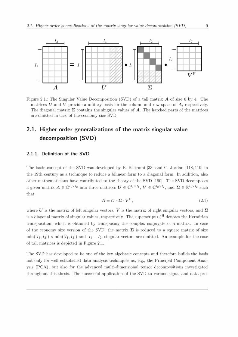
Figure 2.1.: The Singular Value Decomposition (SVD) of a tall matrix A of size 6 by 4. Thematrices U and V provide a unitary basis for the column and row space of A, respectively.The diagonal matrix Σ contains the singular values of A. The hatched parts of the matricesare omitted in case of the economy size SVD.
2.1. Higher order generalizations of the matrix singular value
decomposition (SVD)
2.1.1. Definition of the SVD
The basic concept of the SVD was developed by E. Beltrami [33] and C. Jordan [118, 119] in
the 19th century as a technique to reduce a bilinear form to a diagonal form. In addition, also
other mathematicians have contributed to the theory of the SVD [190]. The SVD decomposes
a given matrix A ∈ CI1×I2 into three matrices U ∈ CI1×I1 , V ∈ CI2×I2 , and Σ ∈ RI1×I2 such
that
A = U ·Σ · V H, (2.1)
where U is the matrix of left singular vectors, V is the matrix of right singular vectors, and Σ
is a diagonal matrix of singular values, respectively. The superscript (·)H denotes the Hermitian
transposition, which is obtained by transposing the complex conjugate of a matrix. In case
of the economy size version of the SVD, the matrix Σ is reduced to a square matrix of size
min([I1, I2])×min([I1, I2]) and |I1 − I2| singular vectors are omitted. An example for the case
of tall matrices is depicted in Figure 2.1.
The SVD has developed to be one of the key algebraic concepts and therefore builds the basis
not only for well established data analysis techniques as, e.g., the Principal Component Anal-
ysis (PCA), but also for the advanced multi-dimensional tensor decompositions investigated
throughout this thesis. The successful application of the SVD to various signal and data pro-

10 2. Multi-dimensional signal decompositions
cessing problems is based on several properties. First, the matrix U provides a unitary basis
(i.e., orthogonal column vectors normalized to unit length) for the column space of A, whereas
the matrix V contains a unitary basis for the row space of A. Second, the diagonal matrix
Σ reflects very important rank-related properties of the matrix A, e.g., it can be determined
whether A is rank deficient (i.e., the rank of A is smaller than min([I1, I2])) or close to a rank
deficient matrix. See the following Section 2.1.2 for further information. A third, and very
important property is that the decomposition is stable in the sense that small perturbations in
A lead only to small perturbations in Σ. Finally, based on the seminal work of G. Golub and
W. Kahan [84] there are fast and numerically stable algorithms available to calculate the SVD.
2.1.2. Properties of the matrix singular value decomposition (SVD)
Many properties of the SVD become evident from its connection to the EigenValue Decompo-
sition (EVD). In order to show this connection we analyze the matrices AAH and AHA with
respect to the SVD of A according to equation (2.1). Since the matrices of left singular vectors
U and right singular vectors V are both unitary, i.e., UUH = I and V V H = I we obtain
A ·AH = UΣV H ·(UΣV H
)H= UΣΣHUH = UΛUH ,
AH ·A =(UΣV H
)H ·UΣV H = V ΣHΣV H = V ΛV H .(2.2)
Here, we can conclude that the matrices U and V contain the eigenvectors of the matrices AAH
and AHA, respectively. The singular values σi, are given by the square root of the eigenvalues λi
of AAH or AHA which are both positive semi-definite matrices. Therefore, the singular values
are non-negative real-valued numbers that have to be sorted in ascending order of magnitude,
yielding
Σ = diag([σ1,σ2, . . . ,σmin({I1,I2})
])
= diag([√
λ1,√λ2, . . . ,
√λmin({I1,I2})
]),
σ1 ≥ σ2 ≥ . . . ≥ σmin([I1,I2]) ≥ 0 .
(2.3)
For more information on eigenvalues, eigenvectors, and the EVD see Appendix C.
One of the most important properties of the SVD is the connection of the singular values to the
matrix rank. If a matrix A ∈ CI1×I2 obeys the matrix rank R = rank(A) then
σi = 0 for all i = R+ 1 . . .min([I1, I2]), (2.4)

2.1. Higher order generalizations of the matrix singular value decomposition (SVD) 11
!"#$%&'()*+,-./0123456789:;<=>?@ABCDEFGHIJKLMNOPQRSTUVWXYZ[\]_abcdefghijklmnopqrstuvwxyz{|}~
=I1 I1
I2 d I2
dd
A U ΣV H
σi
s
Ud
Σd V Hd
Figure 2.2.: The best rank d = 5 approximation of a matrix A of size 10 × 8 based on theSVD. After the determination of the d dominant singular values, all remaining singularvalues are set to zero by simply omitting the hatched parts of the matrices U , V and Σ.The parameter d can be determined by analyzing the singular value profile and choosing anadequate application-dependent threshold parameter s.
i.e., R equals the number of non-zero singular values of A. Furthermore, the problem of iden-
tifying the best low rank approximation Ad of a given matrix A can be solved very efficiently
with the help of the SVD. Thereby, the matrix Ad has to be of rank d while the Mean Square
Error (MSE) with respect to A is minimized
∥A− Ad∥2F → min s.t. rank(Ad
)= d. (2.5)
The solution to this problem has been given by C. Eckart and G. Young in 1936 [77] by con-
structing Ad from the SVD of A considering only the first d dominant singular values (i.e.,
setting the remaining R− d smallest singular values to zero)
Ad = Ud ·Σd · V Hd
= Ud · diag ([σ1,σ2, . . . ,σd]) · V Hd .
(2.6)
Here, Ud ∈ CI1×d and Vd ∈ CI2×d are the matrices of the first d left and right singular vectors,
respectively. The diagonal matrix Σd is of size d× d. In Figure 2.2 the low rank approximation
according to equation (2.6) is visualized for a matrix of size 10 × 8 and d = 5. In practical
applications, e.g., for the noise reduction of multi-variate signals, the choice of d is crucial. It
can be determined by analyzing the singular value profile and choosing a suitable threshold s
such that
d = argmini([σi − s]) s.t. σi ≥ s , (2.7)

12 2. Multi-dimensional signal decompositions
where d is determined as the number of singular values which are greater or equal to s (see
Figure 2.2). The threshold s (or equivalently the number d) can be determined by a number
of Model Order Selection (MOS) techniques among which the Akaike information criterion [22]
is one of the most classical and prominent methods. However, depending on the application,
other MOS algorithms are preferable. For more information about MOS techniques the reader
is referred to [60].
2.1.3. Higher order generalization based on the n-ranks
According to the classical definition, the column rank R = rank(A) is the maximum number
of linear independent column vectors of A. Accordingly, the row rank of a matrix A can be
defined as the maximum number of linear independent row vectors. However, one of the most
fundamental results of linear algebra states that for matrices the column and row rank are always
equal [192], i.e.,
R = rank(A) = rank(AT
). (2.8)
In the following, we generalize the concept of the column and the row rank of a matrix to tensors
(higher order arrays). This is easily achieved be realizing that in the same way as a matrix (i.e., a
two-dimensional (2D) tensor) can be seen as a collection of column and row vectors, a tensor can
be seen as a collection of n-mode vectors. Thereby, the n-mode vectors are obtained by varying
the n-th index within its range in = 1, . . . , In while keeping all other indices fixed. Figure 2.3
visualizes the set of one-mode, two-mode, and three-mode vectors for a tensor of order three and
size 2× 3 × 2. Please recognize that the general concept of n-mode vectors is easily applicable
to matrices, which constitutes that the column vectors of a matrix equal its one-mode vectors,
while the row vectors equal its two-mode vectors. Furthermore, the concept of the column and
row rank of a matrix can be generalized directly to higher-order tensors by defining the n-rank
(in literature also sometimes termed the multi-linear rank or mode-n rank [69]) of a tensor as
the maximum number of linear independent n-mode vectors. By storing all n-mode vectors of
a N -th order tensor X ∈ CI1×···×IN in the columns of a matrix [X ](n) we obtain
Rn = rankn (X ) = rank([X ](n)
), (2.9)
where [X ](n) is a matrix of size In×I1 · . . . ·IN/In named the n-mode unfolding of X . Please note
that in contrast to the matrix case, all n-ranks can be different for tensors of order N ≥ 3 (cf.
Section 2.2.3.2). For more details about the exact construction of the n-mode unfolding including
the order of the n-mode vectors see Appendix A.3. Throughout this work, we consistently use

2.1. Higher order generalizations of the matrix singular value decomposition (SVD) 13
!"#$%&'()*+,-./0123456789:;<=>?@ABCDEFGHIJKLMNOPQRSTUVWXYZ[\]_abcdefghijklmnopqrstuvwxyz{|}~
i1
i2
i3
i1
i2
i3
i1
i2
i3
i1
i2
i3
Figure 2.3.: A third order tensor of size 2 × 3 × 2 and its n-mode vectors. In the same way asmatrices can be seen as a collection of column (vertical) and row (horizontal) vectors, thistensor can be seen as a collection of one-mode (vertical), two-mode (horizontal), and three-mode (lateral) vectors. The thick axis indicate the indices that vary in order to obtain then-mode vectors. The other indices remain fixed.
the MATLAB-like unfolding introduced in [9]. In this unfolding definition, all n-mode vectors
are arranged such that their indices change in ascending order i1, . . . , in−1, in+1, . . . , iN .
In order to generalize the SVD from 2D matrices to a higher order tensor X it is necessary to
transform the n-mode vector space spanned by the n-mode vectors of X . This is achieved by
means of the n-mode product of the tensor X and a transformation matrix U ∈ CJ×In, denoted
by X ×n U . Thereby, the n-mode product is carried out in terms of matrix algebra simply by
multiplying all n-mode vectors of X from the left hand side by the matrix U . Since all n-mode
vectors of X are collected in the columns of the n-mode unfolding matrix of X we obtain
Y = X ×n U ⇐⇒ [Y ](n) = U · [X ](n) . (2.10)
From this relation we can conclude that the n-mode product (2.10) is carried out by building the
n-mode unfolding of X , multiplying it from the left hand side by the matrix U resulting in the
n-mode unfolding of Y. Finally, the resulting tensor Y of size I1× · · ·× In−1×J × In+1 · · ·× IN
has to be reconstructed from its n-mode unfolding matrix [Y](n). Please notice that the number
of rows in U has to match the size of the tensor X along the n-th dimension in order to carry
out the n-mode product (2.10).

14 2. Multi-dimensional signal decompositions
Before generalizing the matrix SVD (2.1), we discuss the equivalence of matrix products and
n-mode products for 2D tensors. Since the product of a matrix A with a matrix U from the
left hand side, i.e., B = U ·A, transforms the column space of A and the column vectors of A
match its one-mode vectors, we can write
B = U ·A
=⇒ [B][1] = U · [A][1]
=⇒ B = A×1 U . (2.11)
In analogy, the row space of a matrix A is transformed by a multiplication with a transformation
matrix V T from the right hand side, i.e., C = A ·V T. Together with AT = [A][2] we can write
C = A · V T
=⇒ CT = V ·AT
=⇒ [C][2] = V · [A][2]
=⇒ C = A×2 V . (2.12)
By utilizing the latter connections between the matrix product and the n-mode product we can
reformulate the matrix SVD (2.1) by
A = U ·Σ · V H
= (Σ×1 U) · V H
= Σ×1 U ×2 V∗
A = Σ×1 U(1) ×2 U
(2) , (2.13)
with U (1) = U and U (2) = V ∗. The representation (2.13) of the SVD can now be generalized
very easily to the Higher Order Singular Value Decomposition (HOSVD) for a N -th order tensor
X ∈ CI1×···×IN by writing
X = S ×1 U(1) ×2 U
(2) ×3 · · ·×N U (N) , (2.14)
where in contrast to the diagonal matrix Σ from (2.13) the tensor S ∈ CI1×···×IN is a full tensor
of the same size as X , also termed the core tensor of the HOSVD. The structure of the HOSVD
according to (2.14) is visualized for the third order case in Figure 2.4. In the same way as
the matrices U and V provide a unitary basis for the row and the column space of A in the
SVD (2.1), the matrices U (n) have to provide a unitary basis for the n-mode vector space of

2.1. Higher order generalizations of the matrix singular value decomposition (SVD) 15
!"#$%&'()*+,-./0123456789:;<=>?@ABCDEFGHIJKLMNOPQRSTUVWXYZ[\]_abcdefghijklmnopqrstuvwxyz{|}~
1
3
2
X U (1) S U (2)
U (3)
Figure 2.4.: The Higher Order Singular Value Decomposition (HOSVD) of a tensor X of size4× 2× 3. In contrast to the matrix case, the core tensor S is a full tensor of the same size asX . The matrices U (1), U (2), and U (3) provide a unitary basis for the one-mode, two-mode,and three-mode vector spaces of X , respectively.
X in the HOSVD (2.14) for n = 1, . . . , N . However, since the n-mode vectors of X are found
in the columns of the n-mode unfoldings [X ](n) we can calculate all matrices U (n) as the left
singular vectors of these unfoldings, i.e.,
[X ](n) = U (n) ·Σ(n) · V (n)H . (2.15)
Therefore, in order to determine the HOSVD of a tensor X of order N , we have calculate N
matrix SVDs to obtain the matrices of n-mode singular vectors U (n) in equation (2.14). In the
sequel, the core tensor S can be determined by rearranging (2.14) to
S = X ×1 U(1)H ×2 U
(2)H ×3 · · · ×N U (N)H . (2.16)
The core tensor S obeys some interesting properties, among which especially the all-orthogonality
property is crucial for the definition of the HOSVD according to (2.14). For a complete investi-
gation of all the properties of the HOSVD we refer to [135]. All properties relevant to this thesis
are discussed in Section 2.2.
2.1.4. Higher order generalization based on the tensor rank
So far, we have stated in Section 2.1.2 that the rank of a matrix equals their maximum number
of linear independent row / column vectors and generalized this fact to the concept of n-ranks

16 2. Multi-dimensional signal decompositions
!"#$%&'()*+,-./0123456789:;<=>?@ABCDEFGHIJKLMNOPQRSTUVWXYZ[\]_abcdefghijklmnopqrstuvwxyz{|}~
=
=
A U
Σ
V H
u1 u2 u3 u4
vH1
vH2
vH3
vH4
u1 u2 u3 u4
vH1 vH
2 vH3 vH
4
Figure 2.5.: The SVD of a matrix A of size 6 × 4 and a rank of R = 4. The SVD can bereformulated as a sum of rank-one matrices, leading to the interpretion of R as the minimumnumber of rank-one matrices that sum up to A.
for higher order tensors in Section 2.1.3, leading to the definition of the HOSVD. Additionally,
we stated that the rank of a matrix A is given by the number of non-zero singular values of A.
However, there is another interpretation on the matrix rank, which is based on the following
alternative representation of the SVD (2.1)
A = U ·Σ · V H =R∑
r=1
σrur · vHr , (2.17)
with U = [u1, . . . ,uR], V = [v1, . . . ,vR], and Σ = diag({σ1, . . . ,σR}). Therefore, the rank
R of a matrix A represents the minimum number of rank-one matrices σrur · vHr which sum
up to A [85, 192]. Thereby, a matrix is of rank-one if and only if it can be represented by
the outer product of two vectors. In Figure 2.5 this interpretation of the matrix rank based on
equation (2.17) is visualized for a matrix A of size 6×4 and a rank of R = 4. This interpretation
of the matrix rank can be generalized directly to higher order tensors and builds the basis
for extending the SVD to the multi-dimensional Parallel Factor (PARAFAC) decomposition.
In order to achieve this, we first define a rank-one tensor Y ∈ CI1×···×IN of order N as a
generalization of the above mentioned definition of a rank-one matrix by
Y = a(1) ◦ a(2) ◦ · · · ◦ a(N) , (2.18)
with a(n) ∈ CIn for n = 1, . . . , N . Therefore, a N -th order tensor Y has tensor rank-one if and
only if it can be represented by the outer product of N vectors. Please notice that the rank-one
tensor according to (2.18) represents a N -dimensional higher order array collecting all possible

2.2. The Higher Order Singular Value Decomposition (HOSVD) 17
!"#$%&'()*+,-./0123456789:;<=>?@ABCDEFGHIJKLMNOPQRSTUVWXYZ[\]^_`abcdefghijklmnopqrstuvwxyz{|}~
a(1)1
a(2)1
a(3)1
a(1)2
a(2)2
a(3)2
a(1)3
a(2)3
a(3)3
X
Figure 2.6.: The PARAFAC Decomposition of a third oder tensor X of size 4 × 3 × 3 and atensor rank of R = 3. The tensor rank represents the minimum number of rank-one tensorsthat sum up to X . Thereby, every rank-one tensor (component) is represented by the outerproduct of three vectors.
N -th order product tupels between the elements a(n)in in the vectors a(n), such that
(Y)i1,i2,...,iN =N∏
n=1
a(n)in. (2.19)
Based on the definition of rank-one tensors according to (2.18), we can now define the tensor
rank R = rank(X ) of an order N tensor X ∈ CI1×···×IN as the minimum number of rank-one
tensors Yr yielding
X =R∑
r=1
Yr =R∑
r=1
a(1)r ◦ a(2)
r ◦ · · · ◦ a(N)r . (2.20)
With the smallest possible number R, equation (2.20) represents the so called Parallel Fac-
tor (PARAFAC) decomposition of the tensor X , which is unique under very mild (i.e., non-
restrictive) conditions. For a detailed discussion of the PARAFAC model see Section 2.3. In
Figure 2.6 the PARAFAC decomposition of a third order tensor of size 4 × 3 × 3 with tensor
rank 3 is visualized. Please note that for N -th order higher order arrays X with N ≥ 3 there
is no direct connection between the n-ranks and the tensor rank of X , such that the HOSVD
according to (2.14) and the PARAFAC decomposition according to (2.20) indeed differ greatly.
2.2. The Higher Order Singular Value Decomposition (HOSVD)
The HOSVD was introduced by L. Lathauwer, B. De Moor, and J. Vandewalle in the year
2000 [135] as a n-rank based generalization of the SVD. Since then, it has found various
applications in different fields of signal and image processing. However, the basic structure of the

18 2. Multi-dimensional signal decompositions
HOSVD as a transformation of the n-mode vector spaces of a tensor has been developed earlier
by L. R. Tucker [196]. Furthermore, the concept of n-ranks was introduced by J. B. Kruskal [130].
For more information about the Tucker decomposition and its history we refer to [128].
Throughout this thesis, the HOSVD is mainly used in order implement the Tucker compression
(cf. Section 2.2.3.3), which represents a technique to reduce the size of multi-dimensional data.
In Section 2.4 the Tucker compression is used in order to reduce the complexity for computing
the PARAFAC2 model parameters. Furthermore, the closed-form PARAFAC algorithm [163,
164] is based on a connection between the HOSVD and the PARAFAC decomposition (cf.
Section 2.3.3.2).
In the following, we define the HOSVD in Section 2.2.1 together with all related parameters and
discuss in particular the all-orthogonality feature, which is characteristically for the HOSVD core
tensor. In the sequel, we summarize the computational algorithm of the HOSVD in Section 2.2.2
before investigating the key properties relevant to this thesis in Section 2.2.3. Thereby, also the
Tucker compression and the algorithm of Higher Order Orthogonal Iterations (HOOI) [136] for
the optimum n-rank reduction of a higher order tensor are discussed.
2.2.1. Definition of the HOSVD
As already derived in Section 2.1.3, the HOSVD of a N -th order tensor X ∈ CI1×···×IN is defined
by
X = S ×1 U(1) ×2 U
(2) ×3 · · ·×N U (N) , (2.21)
where the N -th order tensor S ∈ CI1×···×IN is the core tensor, and the matrices U (n) are the
matrices of n-mode singular vectors of X for n = 1, . . . , N . The matrices U (n) ∈ CIn×In are
obtained by the matrix SVD of the n-mode unfoldings of X
[X ](n) = U (n) ·Σ(n) · V (n)H , (2.22)
and therefore provide a unitary basis for the n-mode vector space of X . Furthermore, the
singular values of the n-mode unfoldings [X ][n] are termed the n-mode singular values of X and
are denoted by σ(n)i with i = 1, . . . , In. After computing the matrices of n-mode singular vectors
according to (2.22), the core tensor S is given by changing (2.21) to
S = X ×1 U(1)H ×2 U
(2)H ×3 · · ·×N U (N)H . (2.23)
2.2. The Higher Order Singular Value Decomposition (HOSVD) 19
!"#$%&'()*+,-./0123456789:;<=>?@ABCDEFGHIJKLMNOPQRSTUVWXYZ[\]_abcdefghijklmnopqrstuvwxyz{|}~
= 12
3
X U (1) S U (2)
U (3)
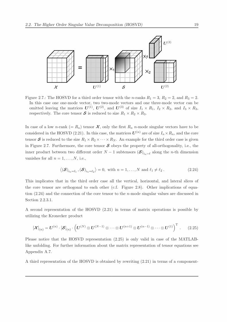
Figure 2.7.: The HOSVD for a third order tensor with the n-ranks R1 = 3, R2 = 2, and R3 = 2.In this case one one-mode vector, two two-mode vectors and one three-mode vector can beomitted leaving the matrices U (1), U (2), and U (3) of size I1 × R1, I2 × R2, and I3 × R3,respectively. The core tensor S is reduced to size R1 ×R2 ×R3.
In case of a low n-rank (= Rn) tensor X , only the first Rn n-mode singular vectors have to be
considered in the HOSVD (2.21). In this case, the matrices U (n) are of size In×Rn, and the core
tensor S is reduced to the size R1×R2× · · ·×RN . An example for the third order case is given
in Figure 2.7. Furthermore, the core tensor S obeys the property of all-orthogonality, i.e., the
inner product between two different order N − 1 subtensors (S)in=ℓ along the n-th dimension
vanishes for all n = 1, . . . , N , i.e.,
⟨(S)in=ℓ1
, (S)in=ℓ2
⟩= 0, with n = 1, . . . , N and ℓ1 = ℓ2 . (2.24)
This implicates that in the third order case all the vertical, horizontal, and lateral slices of
the core tensor are orthogonal to each other (c.f. Figure 2.8). Other implications of equa-
tion (2.24) and the connection of the core tensor to the n-mode singular values are discussed in
Section 2.2.3.1.
A second representation of the HOSVD (2.21) in terms of matrix operations is possible by
utilizing the Kronecker product
[X ](n) = U (n) · [S](n) ·(U (N) ⊗U (N−1) ⊗ · · ·⊗U (n+1) ⊗U (n−1) ⊗ · · · ⊗U (1)
)T. (2.25)
Please notice that the HOSVD representation (2.25) is only valid in case of the MATLAB-
like unfolding. For further information about the matrix representation of tensor equations see
Appendix A.7.
A third representation of the HOSVD is obtained by rewriting (2.21) in terms of a component-

20 2. Multi-dimensional signal decompositions
Algorithm 1 The algorithm for computing the HOSVD of a tensor X according to equa-tion (2.21). Additionally, the n-mode singular values and the n-ranks are computed.
Require: Tensor X of order N and size I1 × I2 × · · ·× IN
• for n = 1, 2, . . . , N
– determine the n-mode unfolding [X ](n) of X
– determine the SVD: [X ](n) = U (n) ·Σ(n) · V (n)H
– determine the n-rank Rn as the number of non-zero diagonal elements in Σ(n)
end
• S = X ×1 U(1)H ×2 U
(2)H ×3 · · ·×N U (N)H
• return n-mode singular vectors U (n) for n = 1, . . . , N
• return core tensor S
• return n-mode singular values Σ(n) = diag(σ(n)1 ,σ(n)2 , . . . ,σ(n)In
)for n = 1, . . . , N
• return n-ranks Rn for n = 1, . . . , N
wise decomposition
X =R1∑
i1=1
R2∑
i2=1
· · ·RN∑
iN=1
si1,i2,...,iN · u(1)i1◦ u(2)
i2◦ · · · ◦ u(N)
iN
=R1∑
i1=1
R2∑
i2=1
· · ·RN∑
iN=1
si1,i2,...,iN · U i1,i2,...,iN ,
(2.26)
where ◦ denotes the outer product, (S)i1,i2,...,iN = si1,i2,...,iN are the elements of the core ten-
sor (2.23), U (n) = [u(n)i1
,u(n)i2
, . . . ,u(n)iN
] are the n-mode singular vectors, and Rn are the n-ranks
of the tensor X , respectively. Therefore, the HOSVD according to (2.26) can be seen as a
superposition of mutually orthogonal rank-one tensors U i1,i2,...,iN .
2.2.2. The computational algorithm for the HOSVD
In Algorithm 1 the necessary steps for computing the HOSVD (2.21) are summarized. This
includes also the computation of the n-mode singular values as well as the n-ranks. Please
notice that instead of using the SVD (2.22) for the computation of the n-mode singular vectors,
also the EigenValue Decomposition (EVD)
[X ](n) · [X ]H(n) = U (n) ·Σ(n) · V (n) ·(U (n) ·Σ(n) · V (n)
)H= U (n) ·Σ(n)2 ·U (n)H (2.27)

2.2. The Higher Order Singular Value Decomposition (HOSVD) 21
can be applied. However, in spite of the significantly reduced amount of data involved in the
EVD (2.27) it is usually considered to be numerically more stable, and hence more accurate, to
calculate the SVD (2.22) directly [85]. Especially in cases where the n-mode unfolding is badly
conditioned (i.e., high ratio between the largest and the smallest singular value) using the SVD
mitigates numerical problems.
From Algorithm 1 it is easily recognized that the computational complexity for the HOSVD of a
tensor of order N equals the complexity of N matrix SVDs. Since there are no extensive iterative
procedures involved in the computation of the HOSVD, it obeys a low complexity compared to
other multi-dimensional decompositions such as PARAFAC or PARAFAC2.
2.2.3. Important properties of the HOSVD
In the following, we discuss the most relevant properties of the HOSVD which are needed in
order to understand the advanced multi-dimensional decomposition techniques used throughout
this thesis. That includes the properties of the core tensor as well as the properties of the of
the n-ranks. Based on this, we also describe the tucker compression method in Section 2.2.3.3
and the best n-rank approximation of a tensor using the algorithm of Higher Order Orthogonal
Iterations (HOOI) in Section 2.2.3.4. For a complete discussion of all properties connected to
the HOSVD we refer to [135].
2.2.3.1. The all-orthogonal core tensor
As already stated in Section 2.2.1, the HOSVD core tensor S ∈ CI1×I2×···×IN is all-orthogonal,
i.e., two different subtensors (S)in=ℓ1and (S)in=ℓ2
, obtained by fixing the n-th index to constant
numbers ℓ1 and ℓ2, are orthogonal to each other in case of ℓ1 = ℓ2 for all n = 1, . . . , N . Since
the elements of the order N − 1 subtensor (S)in=ℓ can be found in the ℓ-th row of the n-mode
unfolding of S, we obtain
[S](n) · [S]H(n) = diag(σ(n)
2
1 ,σ(n)2
2 , . . . ,σ(n)2
IN
)= Σ(n)2 for all n = 1, . . . , N , (2.28)

22 2. Multi-dimensional signal decompositions
!"#$%&'()*+,-./0123456789:;<=>?@ABCDEFGHIJKLMNOPQRSTUVWXYZ[\]_abcdefghijklmnopqrstuvwxyz{|}~
σ(1)
ℓ
σ(2)ℓ
σ(3)ℓ
Si1=ℓ
Si2=ℓ
Si3=ℓ
ℓ
ℓ
ℓ
Figure 2.8.: The all orthogonal slices of a third order core tensor S and the corresponding one-mode, two-mode, and three-mode singular values. All vertical, horizontal, and lateral slicesof S are mutually orthogonal to each other, and the higher order norm of the slices Sin=ℓ
equals the corresponding n-mode singular value σ(n)ℓ .
i.e., all n-mode unfoldings of S have mutually orthogonal rows. The proof for equation (2.28) is
obtained easily by comparing the Kronecker version of the HOSVD (2.25) with (2.22) yielding
Σ(n) · V (n)H = [S](n) ·(U (N) ⊗U (N−1) ⊗ · · · ⊗U (n+1) ⊗U (n−1) ⊗ · · ·⊗U (1)
)T
=⇒ [S](n) = Σ(n) · V (n)H(U (N) ⊗U (N−1) ⊗ · · ·⊗U (n+1) ⊗U (n−1) ⊗ · · ·⊗U (1)
)∗
︸ ︷︷ ︸unitary
, (2.29)
where the fact that the highlighted matrix on the right side of (2.29) is unitary shows that the
Frobenius norm of the rows of [S](n) are given by diagonal elements in Σ(n). Furthermore, we
can conclude that the higher order norm (cf. Appendix A.5) of the subtensors (S)in=ℓ are given
by the n-mode singular values, such that
∥ (S)in=ℓ ∥H = σ(n)ℓ for all ℓ = 1, . . . , In . (2.30)
Since the n-mode singular values in (2.30) are sorted in decreasing order of magnitude, also the
higher order norm (cf. Appendix A.8) of the subtensors of S are sorted
∥ (S)in=1 ∥H ≥ ∥ (S)in=2 ∥H ≥ · · · ≥ ∥ (S)in=In ∥H ∀ n = 1, . . . , N . (2.31)
From the last equation, we can conclude that the scalar elements of S with the highest magnitude
are found at low valued indices i1, i2, . . . , iN . The connection between the subtensors (S)in=ℓ
and the n-mode singular values is visualized in Figure 2.8 for the third order case. Finally, it
can be concluded from (2.29) that the total energy in the tensor X equals the total energy in

2.2. The Higher Order Singular Value Decomposition (HOSVD) 23
!"#$%&'()*+,-./0123456789:;<=>?@ABCDEFGHIJKLMNOPQRSTUVWXYZ[\]_abcdefghijklmnopqrstuvwxyz{|}~
9
9 5
55
5 3
3
replacemen
i1
i2
i3
[X ](1) =
(5 3 9 55 3 9 5
)=⇒ R1 = rank
([X ](1)
)= 1
[X ](2) =
(5 5 9 93 3 5 5
)=⇒ R2 = rank
([X ](2)
)= 2
[X ](3) =
(5 5 3 39 9 5 5
)=⇒ R3 = rank
([X ](3)
)= 2
Figure 2.9.: An example of a third order tensor X with different n-ranks R1 = 1, R2 = 2, andR3 = 2. Notice that in contrast to the matrix case all n-ranks can be different if the order ofthe tensor X exceeds 2.
its core tensor S and is connected to the n-mode singular values by
∥X ∥2H = ∥S∥2H =Rn∑
ℓ=1
(σ(n)ℓ
)2with arbitrary n = 1, . . . , N , (2.32)
where Rn is the n-rank of X . Therefore, the energy of a higher order array is invariant against
unitary n-mode transformations.
2.2.3.2. The n-rank of a tensor
As derived in Section 2.1.3, the n-rank Rn of a tensor X ∈ CI1×···×IN is the maximum number
of linear independent n-mode vectors, i.e., the dimension of the n-mode vector space, which can
be computed simply by the matrix rank of the n-mode unfolding
Rn = rank([X ](n)
)≤ In . (2.33)
At this point it is crucial to notice that in contrast to the matrix case, where the column rank
always equals the row rank, all the n-ranks of a N -th order tensor can be different if N ≥ 3. An
example for a third order tensor with different R1 and R2 is depicted in Figure 2.9. Another
important difference in the properties of higher order n-ranks compared to the matrix case is
realized by considering the problem of the best low n-rank approximation of a given tensor X .
The best low n-rank approximation X of a tensor X in least squares sense has to fulfill
∥X − X ∥2H → min s.t. rank
([X]
(n)
)= dn , (2.34)

24 2. Multi-dimensional signal decompositions
!"#$%&'()*+,-./0123456789:;<=>?@ABCDEFGHIJKLMNOPQRSTUVWXYZ[\]_abcdefghijklmnopqrstuvwxyz{|}~
=1 2
3
X U (1) S U (2)
U (3)
σ(1) σ(3)
σ(2)
Figure 2.10.: The Tucker compression of a third order tensor utilizing the truncated HOSVD.The resulting tensor X obeys the n-ranks d1 = 5, d2 = 4, and d3 = 3. This is obtained byconsidering only the first dn n-mode singular vectors. The relevant size of the core tensor isreduced to d1 × d2 × d3.
with some given n-ranks dn of X for all n = 1, . . . , N . In the matrix case (i.e., N = 2) the solution
to this problem can be created simply by omitting the singular vectors corresponding to the R−dsmallest singular values (cf. the Eckart-Young theorem, Section 2.1.2). However, in the multi-
dimensional case (i.e., for N ≥ 3) the n-mode equivalent of this method (cf. Section 2.2.3.3) does
not create the optimal solution to (2.34) in least squares sense. The Higher Order Orthogonal
Iterations (HOOI) [136] method solving this problem is presented in Section 2.2.3.4.
2.2.3.3. The truncated HOSVD
The general problem of approximating a given tensor X by a tensor X with the maximum n-
ranks d1, d2, . . . , dN is sometimes also termed Tucker compression in literature [112]. As already
stated at the end of the last section, the direct generalization of the Eckart-Young theorem
for computing the best low rank matrix (see Section 2.1.2, equation (2.6)) does not lead to an
optimal solution in the higher order case. However, computing a low n-rank approximation
of the tensor X simply by truncating the HOSVD, i.e., considering only the first dn n-mode
singular vectors corresponding to the dn largest n-mode singular values, constitutes a very fast
approximate solution to the problem (2.34)
X = S ′ ×1 U(1)′ ×2 U
(2)′ ×3 · · ·×N U (N)′ . (2.35)
Here, the matrices U (n)′ =[u(n)1 ,u(n)
2 , . . . ,u(n)dn
]are the matrices of dn dominant n-mode sin-
gular vectors obtained from (2.22) and the truncated core tensor S ′ of size d1× d2× · · ·× dN is

2.2. The Higher Order Singular Value Decomposition (HOSVD) 25
Algorithm 2 The algorithm for computing the truncated HOSVD of a tensor X of size I1 ×· · ·× IN and the n-ranks dn according to equation (2.35).
Require: Tensor X of order N and the n-ranks dn for n = 1, . . . , N of XEnsure: dn ≤ In for all n = 1, . . . , N
• for n = 1, 2, . . . , N
– determine the n-mode unfolding [X ](n) of X
– determine the SVD: [X ](n) = U (n) ·Σ(n) · V (n)H
– determine the matrices of dn dominant n-mode singular vectors U (n)′ =[u(n)1 ,u(n)
2 , . . . ,u(n)dn
]
end
• S = X ×1 U(1)H ×2 U
(2)H ×3 · · ·×N U (N)H
• create S ′ ∈ Cd1×···×dn by (S ′)i1,i2,...,iN = (S)i1,i2,...,iN for in = 1, . . . , dn
• return dn dominant n-mode singular vectors U (n)′ for n = 1, . . . , N
• return truncated core tensor S ′
constructed from the elements of the core tensor S (2.23) by
(S′)
i1,i2,...,iN= (S)i1,i2,...,iN for all in = 1, . . . , dn . (2.36)
The low n-rank approximation X according to (2.35) has the n-ranks dn and is termed the
truncated HOSVD [112]. The structure of the truncated HOSVD in case of a third order
tensor with d1 = 5, d2 = 4, and d3 = 3 is depicted in Figure 2.10 and the computational
steps are summarized in Algorithm 2. Although the approximation (2.35) is in general not
optimal according to the least squares criterium (2.34) it has found many applications and its
performance is often adequate [112]. The truncated HOSVD can be used to obtain a good
starting point for iterative algorithms solving (2.34), such as the HOOI method presented in
Section 2.2.3.4. Furthermore, it is used throughout this thesis as the first computational step in
the closed-form PARAFAC Algorithm 2.3.3.2 and for the estimation of the PARAFAC2 model
parameters in 2.4.3.2.
2.2.3.4. Optimal n-rank approximation using Higher Order Orthogonal Iterations (HOOI)
The Higher Order Orthogonal Iterations (HOOI) algorithm discussed in this section was devel-
oped by L. de Lathauwer, B. de Moore, and J. Vandewalle in 2000 [136], as a generalization of
the well known orthogonal iteration method for matrices [85]. The following explanations are

26 2. Multi-dimensional signal decompositions
based on [136]. The HOOI algorithm aims at finding an optimal solution for the low n-rank
approximation X of a given tensor X according to (2.34), where the fact that all n-ranks of X
are dn leads to
X = SO ×1 U(1)O ×2 U
(2)O ×3 · · ·×N U
(N)O . (2.37)
Here, the unitary matrices U (n)O are of size In × dn while the tensor SO is of size d1 × · · ·× dN .
Assuming that the optimal matrices U (n)O are found, the tensor SO is easily computed by
SO = X ×1 U(1)H
O ×2 U(2)H
O ×3 · · ·×N U(N)H
O , (2.38)
since this is the least squares solution to the set of equations X = SO ×1 U(1)O ×2 · · · ×N U
(N)O .
Furthermore, it can be shown that the least squares condition in (2.34) can be reformulated to
∥X − X∥2H = ∥X ∥2H − ∥SO∥2H , (2.39)
i.e., the solution to the optimization problem (2.34) is achieved by determining the unitary
matrices U (n)O which maximize the norm of SO
∥∥∥X ×1 U(1)H
O ×2 U(2)H
O ×3 · · ·×N U(N)H
O
∥∥∥2
H→ max . (2.40)
For the proof of equation (2.39) the reader is referred to [136]. The solution to the maximization
problem (2.40) can be achieved by means of alternating least squares iterations. In order to do
this we assume that all the matrices U (1)O , . . . ,U (n−1)
O U(n+1)O , . . . ,U (N)
O are fixed and we search
for the single unitary matrix U(n)O that fulfills (2.40). By introducing the tensor Z(n) that
comprises all fixed terms in (2.40) we can write
∥∥∥X ×1 U(1)H
O · · ·×n−1 U(n−1)H
O ×n+1 U(n+1)H
O · · ·×N U(N)H
O ×n U(n)H
O
∥∥∥2
H=
∥∥∥Z(n) ×n U(n)H
O
∥∥∥2
H
=⇒∥∥∥∥U
(n)H
O ·[Z(n)
]
(n)
∥∥∥∥2
F
→ max s.t. U (n)H
O ·U (n)O = I . (2.41)
The solution to the problem (2.41) is known in matrix algebra [85] and given by the matrix of
dn dominant singular vectors of the n-mode unfolding of Z(n)
[Z(n)
]
(n)= UΣV H
=⇒ U(n)O = [u1,u2, . . . ,udn ] , (2.42)
where the vectors un are the columns of the matrix U . By iterating over alternating estimates
according to (2.42) for n = 1, . . . , N the optimization problem (2.34) can be solved. However,

2.2. The Higher Order Singular Value Decomposition (HOSVD) 27
Algorithm 3 The HOOI algorithm according to [136]. The algorithm determines the best low n-rank approximation for given n-ranks d1, d2, . . . , dN of an N -th order tensor X by solving (2.34)with the help of an alternating least squares algorithm.
Require: Tensor X of order N and the n-ranks dn for n = 1, . . . , N of XEnsure: dn ≤ Rn ≤ In for all n = 1, . . . , N
• initialize U (n)′ as the dn dominant n-mode singular vectors of X for n = 2, . . . , N
• repeat
– for n = 1, 2, . . . , N
∗ determine Z(n) = X ×1 U′(1)H · · ·×n−1 U
′(n−1)H ×n+1 U′(n+1)H · · ·×N U ′(N)H
∗ determine the SVD of the n-mode unfolding[Z(n)
]
(n)= UΣV H
∗ consider only the dn dominant singular vectors U (n)′ ← [u1,u2, . . . ,udn ]
end
• until convergence
• determine S′ = Z(N) ×N U ′(N)H
• determine X = S ′ ×1 U′(1) ×2 · · ·×N U ′(N)
• return U (n)′ for n = 1, . . . , N
• return truncated core tensor S ′
• return X
global convergence is is not guaranteed. For the initialization of the iteration process, the
truncated HOSVD (cf. Section 2.2.3.3) yields good starting points for the matrices U(n)O . The
HOOI algorithm is used throughout this thesis as an important tool in order to compute the
best rank-one approximation of a tensor. This is utilized, e.g., in the least-squares Khatri-Rao
factorization Algorithm 12. All necessary steps for computing the best low n-rank approximation
using the HOOI method are summarized in Algorithm 3.
2.2.4. Applications of the HOSVD
Since its introduction in the year 2000, the HOSVD has been used in a variety of applications
throughout very different fields of signal processing. L. de Lathauwer and J. Vandewalle [70]
have considered the application of the truncated HOSVD and the HOOI as a preprocessing
step for the dimensionality reduction of many multi-linear signal processing algorithms, e.g.,
the ICA. Thereby, the computational complexity can be significantly reduced. This subject is
further investigated in [112,113].
Furthermore, the HOSVD has been applied to a number of problems in Multiple Input Multiple

28 2. Multi-dimensional signal decompositions
Output (MIMO) communications. In [9] M. Weis, G. del Galdo, and M. Haardt have introduced
a multi-linear analytical channel model based on the HOSVD of the channel correlation tensor,
providing an improved modeling accuracy in comparison to 2D models. Such channel models
have found many applications in mobile communication systems [3, 10]. Additionally, in [66,
90, 166] it has been shown that it is favorable to preserve the multi-dimensional structure of
channel measurements in order to improve the subspace estimation using the HOSVD. These
results have been confirmed by a theoretical performance analysis in [8]. Finally, Model Order
Selection (MOS) techniques based on the concept of global eigenvalues have been developed
for multi-dimensional harmonic retrieval problems in [65] as well as for the PARAllel FACtor
(PARAFAC) model in [64]. Thereby, the global eigenvalues are derived from the n-mode singular
values of the HOSVD.
In 2002 M. A. O. Vasilescu and D. Terzopoulos [198] introduced the HOSVD to the field of
image processing and computer vision by defining the concept of tensor faces [128]. Thereby,
tensor faces are a multi-linear HOSVD based extension of eigen-faces used in face recognition
algorithms. For this, facial image data of multiple subjects taken in a variety of environmental
conditions are analyzed. These environmental conditions are used as tensor modes, e.g., person,
lighting condition, pixel, camera angle, and others. Incorporating these dimensions in a multi-
linear analysis using tensor faces provides a better face recognition accuracy [199]. Moreover,
tensor faces have been utilized in order to extract facial features while mitigating environmental
effects such as lightning [200]. Additionally, the HOSVD has also been used in the context of
human motion [197], for the analysis of facial expressions [207] and for the compression of image
data [208]. Further applications of the HOSVD are found in the field of data mining [128], e.g.,
the classification of handwritten digits [170], the analysis of chatroom communications [20], and
the improvement of personalized web search data [193].
Throughout this thesis, the truncated HOSVD is used as a preprocessing step in order to re-
duce the amount of data involved in the estimation of the PARAFAC2 model parameters (cf.
Section 2.4). Furthermore, a connection between the HOSVD and the PARAFAC decompo-
sition is exploited by the closed-form PARAFAC algorithm for the efficient computation of
PARAFAC [163, 164]. Also the computation of the Khatri-Rao Factorization (KRF), which
is used for the Procrustes estimation and Khatri-Rao factorization (ProKRaft) algorithm in
Section 2.3.3.3, is based on the truncated HOSVD.
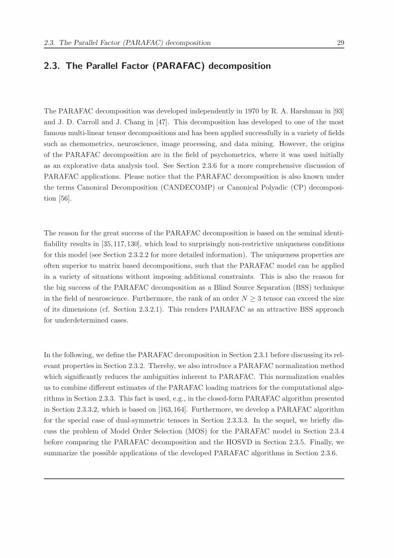
2.3. The Parallel Factor (PARAFAC) decomposition 29
2.3. The Parallel Factor (PARAFAC) decomposition
The PARAFAC decomposition was developed independently in 1970 by R. A. Harshman in [93]
and J. D. Carroll and J. Chang in [47]. This decomposition has developed to one of the most
famous multi-linear tensor decompositions and has been applied successfully in a variety of fields
such as chemometrics, neuroscience, image processing, and data mining. However, the origins
of the PARAFAC decomposition are in the field of psychometrics, where it was used initially
as an explorative data analysis tool. See Section 2.3.6 for a more comprehensive discussion of
PARAFAC applications. Please notice that the PARAFAC decomposition is also known under
the terms Canonical Decomposition (CANDECOMP) or Canonical Polyadic (CP) decomposi-
tion [56].
The reason for the great success of the PARAFAC decomposition is based on the seminal identi-
fiability results in [35,117,130], which lead to surprisingly non-restrictive uniqueness conditions
for this model (see Section 2.3.2.2 for more detailed information). The uniqueness properties are
often superior to matrix based decompositions, such that the PARAFAC model can be applied
in a variety of situations without imposing additional constraints. This is also the reason for
the big success of the PARAFAC decomposition as a Blind Source Separation (BSS) technique
in the field of neuroscience. Furthermore, the rank of an order N ≥ 3 tensor can exceed the size
of its dimensions (cf. Section 2.3.2.1). This renders PARAFAC as an attractive BSS approach
for underdetermined cases.
In the following, we define the PARAFAC decomposition in Section 2.3.1 before discussing its rel-
evant properties in Section 2.3.2. Thereby, we also introduce a PARAFAC normalization method
which significantly reduces the ambiguities inherent to PARAFAC. This normalization enables
us to combine different estimates of the PARAFAC loading matrices for the computational algo-
rithms in Section 2.3.3. This fact is used, e.g., in the closed-form PARAFAC algorithm presented
in Section 2.3.3.2, which is based on [163,164]. Furthermore, we develop a PARAFAC algorithm
for the special case of dual-symmetric tensors in Section 2.3.3.3. In the sequel, we briefly dis-
cuss the problem of Model Order Selection (MOS) for the PARAFAC model in Section 2.3.4
before comparing the PARAFAC decomposition and the HOSVD in Section 2.3.5. Finally, we
summarize the possible applications of the developed PARAFAC algorithms in Section 2.3.6.

30 2. Multi-dimensional signal decompositions
2.3.1. Definition of the PARAFAC decomposition
As derived in Section 2.1.4 the PARAFAC decomposition of a given N -th order tensor X ∈CI1×···×IN is represented by
X =R∑
r=1
Yr =R∑
r=1
a(1)r ◦ a(2)
r ◦ · · · ◦ a(N)r , (2.43)
where R is the tensor rank of X . Thereby, the tensor rank R is defined as the minimum
number of rank-one tensors Yr which fulfill (2.43). The structure of this representation of the
PARAFAC decomposition is visualized in Figure 2.6 for a tensor of order three. The vectors
a(n)r are termed n-mode loading vectors. By collecting all PARAFAC n-mode loading vectors in
the n-mode loading matrices A(n) = [a(n)1 ,a(n)
2 , . . . ,a(n)R ] for n = 1, . . . , N and by utilizing the
n-mode product (cf. Appendix A.4), we can reformulate equation (2.43) to [163]
X = IN,R ×1 A(1) ×2 A
(2) ×3 · · ·×N A(N) . (2.44)
Here IN,R denotes the order N identity tensor of size R along each dimension, such that
(IN,R)i1,i2,...,iN =
⎧⎨
⎩1 for i1 = i2 = · · · = iN
0 otherwise, (2.45)
with in = 1, . . . , R for all indices n = 1, . . . , N . All n-mode loading matrices A(n) are of size
In ×R. The representation (2.44) of the PARAFAC decomposition is visualized in Figure 2.11
for a third order tensor of size 5×4×3 and tensor rank 4. Please notice that this way of writing
PARAFAC is of particular interest, since it is comparable to the structure of the HOSVD (2.21).
This is exploited, e.g., in the closed-form PARAFAC algorithm in Section 2.3.3.2.
Similar to the HOSVD in (2.21), PARAFAC can be expressed with the help of the Kronecker
product (2.25) as
[X ](n) = A(n) · [I ](n) ·(A(N) ⊗A(N−1) ⊗ · · · ⊗A(n+1) ⊗A(n−1) ⊗ · · ·⊗A(1)
)T
= A(n) ·(A(N) ⋄A(N−1) ⋄ · · · ⋄A(n+1) ⋄A(n−1) ⋄ · · · ⋄A(1)
)T, (2.46)
where ⋄ denotes the Khatri-Rao product (cf. Appendix B.3). Please notice that this represen-
tation of PARAFAC is only valid for the MATLAB-like n-mode unfolding (cf. Appendix A.3).
The matrix based PARAFAC representation (2.46) builds the basis for the iterative Alternating

2.3. The Parallel Factor (PARAFAC) decomposition 31
!"#$%&'()*+,-./0123456789:;<=>?@ABCDEFGHIJKLMNOPQRSTUVWXYZ[\]_abcdefghijklmnopqrstuvwxyz{|}~
= 12
3
X A(1) I3,4 A(2)
A(3)
Figure 2.11.: The PARAFAC representation of a third order tensor X of size 5× 4× 3 utilizingthe identity tensor I3,4 and the n-mode product to the n-mode loading matrices A(n). Thegrey shaded values of the identity tensor I3,4 are one while all other elements are zero. Inthis example the tensor rank of X is 4.
Least Squares (ALS) algorithms discussed in Section 2.3.3.1.
In the special case of a third order tensor the PARAFAC model X = IN,R×1A(1)×2A
(2)×3A(3)
can be formulated in terms of the frontal slices of the tensor X and the tensor of diagonal frontal
slices IN,R ×3 A(3). This leads to
(X )i3=ℓ = A(1) ·(I3,R ×3 A
(3))
i3=ℓ·A(2)T , (2.47)
where (·)i3=ℓ denotes the N − 1 dimensional subtensor obtained by keeping the third index i3
fixed to ℓ (hence the ℓ-th frontal slice in the third order case). All discussed representations of
the PARAFAC decomposition are summarized in Table 2.1.
2.3.2. Important properties of the PARAFAC model
In this section, we discuss the properties of the PARAFAC decomposition that are relevant for
this thesis, i.e., the properties of the tensor rank, PARAFAC uniqueness properties, and the
problem of the low rank approximation of a tensor. Especially the properties of the tensor
rank as well as the uniqueness properties show that the PARAFAC decomposition is often
superior in comparison to its matrix-based counterparts (i.e., the SVD). We also present a
novel normalization procedure for the PARAFAC decomposition [16], which reduces its inherent
ambiguities. Moreover, we discuss the properties of PARAFAC for different kinds of symmetric
tensors. Please note that this section does not cover all details of the different PARAFAC

322.
Multi-d
imen
sional
signal
decom
position
s
N-th order model equation Third order model equation Visualized 3D structure
X =R∑
r=1
a(1)r ◦ a(2)
r ◦ · · · ◦ a(N)r X =
R∑
r=1
a(1)r ◦ a(2)
r ◦ a(3)r
!"#$%&'()*+,-./0123456789:;<=>?@ABCDEFGHIJKLMNOPQRSTUVWXYZ[\]^_`abcdefghijklmnopqrstuvwxyz{|}~
a(1)1
a(2)1
a(3)1
a(1)2
a(2)2
a(3)2
a(1)3
a(2)3
a(3)3X
X = IN,R×1A(1)×2A
(2)×3 · · ·×N A(N) X = IN,R ×1 A(1) ×2 A
(2) ×3 A(3)
!"#$%&'()*+,-./0123456789:;<=>?@ABCDEFGHIJKLMNOPQRSTUVWXYZ[\]_abcdefghijklmnopqrstuvwxyz{|}~
= 12
3
X A(1)
I3,4 A(2)
A(3)
[X ](n) = A(n) ·(A(N) · · · ⋄A(n+1) ⋄A(n−1) · · · ⋄A(1)
)T
[X ](1) = A(1) ·(A(3) ⋄A(2)
)T
[X ](2) = A(2) ·(A(3) ⋄A(1)
)T
[X ](3) = A(3) ·(A(2) ⋄A(1)
)T-
- (X )i3=ℓ = A(1) ·(I3,R ×3 A
(3))
i3=ℓ·A(2)T
!"#$%&'()*+,-./0123456789:;<=>?@ABCDEFGHIJKLMNOPQRSTUVWXYZ[\]^_`abcdefghijklmnopqrstuvwxyz{|}~
=
X A(1)
I3,4 ×3 A(3)
A(2)H
Table 2.1.: Overview of possible PARAFAC representations.

2.3. The Parallel Factor (PARAFAC) decomposition 33
properties. For more in depth investigations on this subject, the interested reader is referred
to [56,128] and the references therein.
2.3.2.1. The tensor rank
As already mentioned above, the tensor rank R of a tensor X is the minimum number of rank-
one tensors Yr that sum up to X . In other words, it is the minimum number R for which the
PARAFAC decomposition (2.43) is exactly fulfilled. Although the concept of the tensor rank
can be derived as a generalization of the matrix rank (cf. Section 2.1.4) it obeys considerably
different properties. There is also no direct connection between the n-ranks Rn of a tensor
and its tensor rank R. The only straight forward relation between Rn and R can be concluded
by comparing the component-wise representation of the HOSVD (2.26) and the PARAFAC
model (2.43). This leads to a very loose upper and lower bound for the tensor rank
minn
(Rn) ≤ R ≤N∏
n=1
Rn , (2.48)
where N is the order of the tensor X . In case of third order tensors X ∈ RI1×I2×I3 the following
weak upper bound on the tensor rank has been derived in [130]
rank (X ) ≤ min (I1 · I2, I1 · I3, I2 · I3) . (2.49)
Exact values for the maximum rank of arbitrary tensors of third order have only been derived
for tensors of specific sizes. One of the most general results for the maximum rank Rmax is for
third order tensors X ∈ RI1×I2×2 with only 2 slices [130]
Rmax = min(I1, I2) + min
(I1, I2,
⌊max(I1, I2)
2
⌋). (2.50)
The values of the maximum ranks according to this equation are shown in Table 2.2. From
this table, we can conclude that the tensor rank can exceed the size of the tensor along each
dimension. This important feature of the tensor rank is not found in the matrix case, since the
rank of a matrix A ∈ CI×J is upper bounded by min(I, J). This property of the tensor rank and
consequently the PARAFAC decomposition, gives rise to the application of PARAFAC also in
underdetermined cases of BSS problems. A prominent example is the application of PARAFAC
for the calculation of the underdetermined ICA (i.e., the number of sources exceed the number
of sensors) by diagonalizing the higher order cumulant tensor (cf. Section 2.3.3.3). A major
drawback of the tensor rank is that the problem of identifying it for a given tensor X is of

34 2. Multi-dimensional signal decompositions
I2 = 2 I2 = 3 I2 = 4 I2 = 5 I2 = 6 I2 = 7 I2 = 8
I1 = 2 3 3 4 4 4 4 4I1 = 3 3 4 5 5 6 6 6I1 = 4 4 5 6 6 7 7 8I1 = 5 4 5 6 7 8 8 9I1 = 6 4 6 7 8 9 9 10I1 = 7 4 6 7 8 9 10 11I1 = 8 4 6 8 9 10 11 12
Table 2.2.: Maximum rank of third order 2-slice tensors of size I1 × I2 × 2. The boldface valueshighlight the maximum ranks that exceed the sizes of the tensor along each dimension [130].
non-deterministic polynomial time (NP)-hard [98]. Therefore, the Model Order Selection (i.e.,
identification of the tensor rank under noisy conditions) for the PARAFAC decomposition (cf.
Section 2.3.4) is usually achieved by calculating the PARAFAC decomposition for a number of
candidate model orders until a good fit to the tensor X is achieved. There are a number of
further very interesting properties of the tensor rank which are not found in the matrix case,
e.g., the tensor rank of a real-valued tensor can differ over R and C. For more information on
this subject we refer to [58,128].
2.3.2.2. Uniqueness properties
As already mentioned above, the PARAFAC decomposition (2.43) shows some uniqueness prop-
erties which are superior to the matrix case. This becomes clear by realizing that the matrix
SVD (2.17) is unique only under the additional constraint that its rank-one components are
orthogonal to each other. Furthermore, all its singular values have to be distinct. Contrary,
the PARAFAC decomposition is unique under very mild (i.e., non-restrictive) conditions with-
out imposing an orthogonality constraint. The decomposition (2.43) of X is considered to be
unique if there is only one possible combination of rank-one tensors Yr that sum up to X for
minimal tensor rank R. There has been a lot of effort in finding concrete terms under which the
PARAFAC model is unique, especially by N. D. Sidiropoulos and R. Bro [182], which also provide
some history on the uniqueness results of PARAFAC. The most famous sufficient uniqueness
condition for PARAFAC was given by J. B. Kruskal [129] in 1977 for third order tensors
rankK(A(1)
)+ rankK
(A(2)
)+ rankK
(A(3)
)≥ 2R + 2 , (2.51)
where rankK (·) denotes the Kruskal rank of a matrix and R is the tensor rank. The Kruskal
rank RK of a matrix A is the maximum number RK such that any arbitrary combination

2.3. The Parallel Factor (PARAFAC) decomposition 35
of column vectors of A is linearly independent (cf. Appendix B.6 for examples). From the
Kruskal condition we can conclude that a third order PARAFAC decomposition is not unique
if merely one of the three loading matrices has matrix rank-one. This is because the Kruskal
rank is upper bounded by the matrix rank rankK(A) ≤ rank(A) and equation (2.51) becomes
R+R+ 1 = 2R+ 1 ≥ 2R+ 2 in this case. This result has also implications on the separability
of EEG sources in Chapter 4. The equation (2.51) has been generalized in [182] to the following
sufficient uniqueness condition for the PARAFAC decomposition (2.43) of order N tensors
N∑
n=1
rankK(A(n)
)≥ 2R+ (N − 1) . (2.52)
Other necessary conditions for the uniqueness of PARAFAC have been identified in literature,
from which the most general one is [128,137]
minm=1,...,N
⎛
⎜⎝N∏
n=1m=n
rank(A(n)
)⎞
⎟⎠ ≥ R . (2.53)
2.3.2.3. Low rank approximations
As already stated in Section 2.1.2 the best low rank d approximation Ad of a matrix A according
to the Eckart-Young theorem (2.6) is found by considering only the first d components of the
SVD corresponding to the largest singular values [77]
A =R∑
r=1
σrur · vHr =⇒ Ad =
d∑
r=1
σrur · vHr with σ1 ≥ · · · ≥ σR , (2.54)
where σr are the singular values, ur are the left sided singular vectors and vr are the right
sided singular vectors. Unfortunately, the best low rank approximation X of a tensor X in least
squares sense for orderN ≥ 3 is not given by the higher order generalization of equation (2.54). If
for example, we consider a rank-two tensor X with the PARAFAC decomposition X = Y1+Y2,
then the best rank-one approximation X of X in least squares sense (i.e., ∥X − X ∥2H → min)
is usually neither given by Y1 nor by Y2. As a consequence of this property, it is not possible
to determine the rank-one components of PARAFAC sequentially, e.g., by computing a series of
R best rank-one approximations of the original rank-R tensor X . By contrast, all PARAFAC
components Yr have to be determined jointly.
The best rank-one approximation of a tensor X can be found by using the Higher Order Orthog-

36 2. Multi-dimensional signal decompositions
onal Iterations (HOOI) Algorithm 3 in Section 2.2.3.4 by setting all n-ranks dn to one. In this
case, the HOOI algorithm reduces to the higher order power iteration algorithm also introduced
in [136]. In general, this is possible since a tensor of order N and tensor rank-one implies that
all n-ranks equal one for n = 1, . . . , N and vice verca.
A difficult problem concerning the low rank approximation of a higher order tensor X is de-
generacy, which has again no equivalent in the matrix case. A tensor X of rank R is termed
degenerate, if there exists a series of low rank tensors that approximate X arbitrarily well. Since
the space of rank R tensors is not closed, a unique best low rank approximation of an degenerate
tensor might not even exist. See [128] and references therein for more information about this
subject.
2.3.2.4. Normalization of the PARAFAC model
In this section, we introduce the concept of PARAFAC component amplitudes in order to normal-
ize the decomposition (2.43) and to overcome its inherent permutation and scaling ambiguities.
This is crucial, e.g., for the combination of different estimates of the loading matrices A(n) in
order to identify an improved PARAFAC fit according to equation (2.44). For example, in Sec-
tion 2.3.3.2 the normalization presented here is used to combine the multiple estimates of the
loading matrices A(n) computed by the Closed-Form PARAFAC (CFP) algorithm.
The permutation ambiguity in the PARAFAC model is reflected by the fact that the order
of the rank-one tensors in (2.43) can be changed arbitrarily. The scaling ambiguity implies
that the PARAFAC loading vectors a(n)r can be multiplied by arbitrary constants αn obeying
α1 · α2 · · · · · αN = 1, such that
X =R∑
r=1
a(1)r ◦ a(2)
r ◦ · · · ◦ a(N)r =
R∑
r=1
(α1a
(1)r
)◦(α2a
(2)r
)◦ · · · ◦
(αNa(N)
r
). (2.55)
In order to overcome the scaling ambiguity, we normalize all PARAFAC loading vectors a(n)r to
unit Frobenius norm
a′(n)r =
a(n)r∥∥∥a(n)r
∥∥∥F
for all r = 1, . . . , R and n = 1, . . . , N . (2.56)
Please notice that this implies that all PARAFAC rank-one tensors Y ′r = a
′(1)r ◦a′(2)
r ◦ · · · ◦a′(N)r
have unit tensor norm (cf. Appendix A.5). Using this normalization, we can introduce the
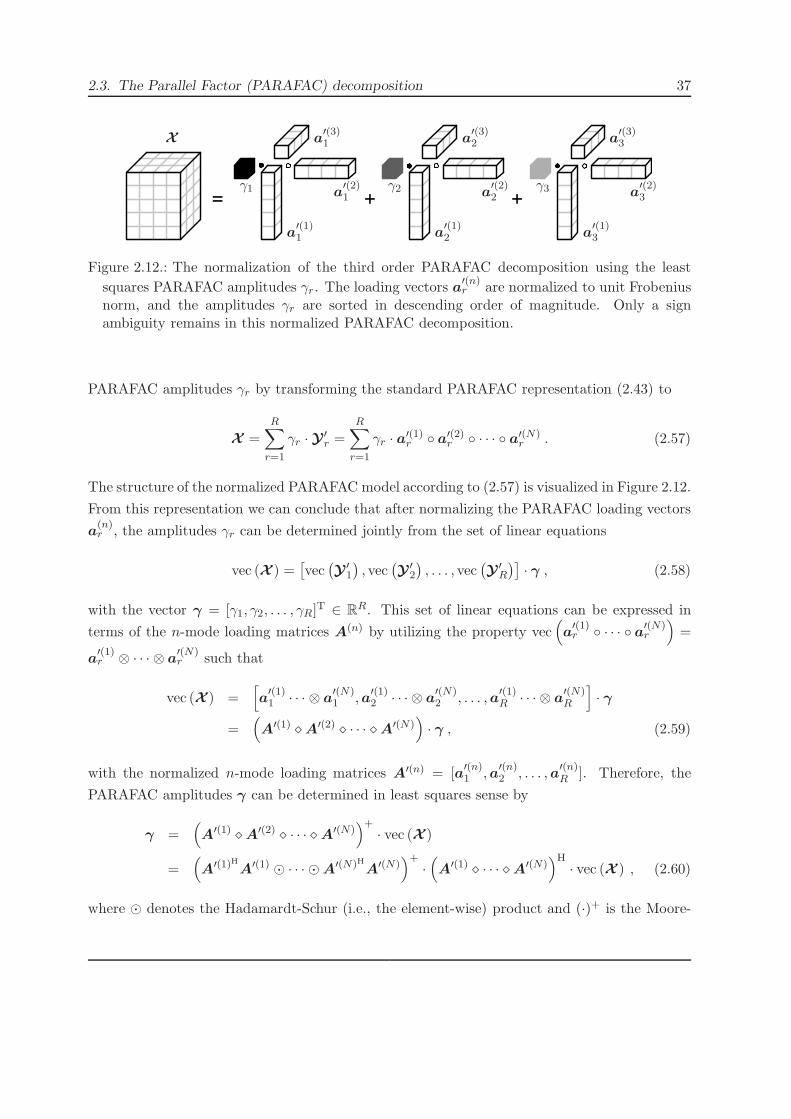
2.3. The Parallel Factor (PARAFAC) decomposition 37
!"#$%&'()*+,-./0123456789:;<=>?@ABCDEFGHIJKLMNOPQRSTUVWXYZ[\]^_`abcdefghijklmnopqrstuvwxyz{|}~
= + +
X
a′(1)1 a
′(1)2 a
′(1)3
a′(2)1 a
′(2)2 a
′(2)3
a′(3)1 a
′(3)2 a
′(3)3
γ1 γ2 γ3
Figure 2.12.: The normalization of the third order PARAFAC decomposition using the least
squares PARAFAC amplitudes γr. The loading vectors a′(n)r are normalized to unit Frobenius
norm, and the amplitudes γr are sorted in descending order of magnitude. Only a signambiguity remains in this normalized PARAFAC decomposition.
PARAFAC amplitudes γr by transforming the standard PARAFAC representation (2.43) to
X =R∑
r=1
γr · Y ′r =
R∑
r=1
γr · a′(1)r ◦ a′(2)
r ◦ · · · ◦ a′(N)r . (2.57)
The structure of the normalized PARAFAC model according to (2.57) is visualized in Figure 2.12.
From this representation we can conclude that after normalizing the PARAFAC loading vectors
a(n)r , the amplitudes γr can be determined jointly from the set of linear equations
vec (X ) =[vec
(Y ′
1
), vec
(Y ′
2
), . . . , vec
(Y ′
R
)]· γ , (2.58)
with the vector γ = [γ1, γ2, . . . , γR]T ∈ RR. This set of linear equations can be expressed in
terms of the n-mode loading matrices A(n) by utilizing the property vec(a′(1)r ◦ · · · ◦ a′(N)
r
)=
a′(1)r ⊗ · · · ⊗ a
′(N)r such that
vec (X ) =[a′(1)1 · · · ⊗ a
′(N)1 ,a′(1)
2 · · ·⊗ a′(N)2 , . . . ,a′(1)
R · · ·⊗ a′(N)R
]· γ
=(A′(1) ⋄A′(2) ⋄ · · · ⋄A′(N)
)· γ , (2.59)
with the normalized n-mode loading matrices A′(n) = [a′(n)1 ,a′(n)
2 , . . . ,a′(n)R ]. Therefore, the
PARAFAC amplitudes γ can be determined in least squares sense by
γ =(A′(1) ⋄A′(2) ⋄ · · · ⋄A′(N)
)+· vec (X )
=(A′(1)HA′(1) ⊙ · · ·⊙A′(N)HA′(N)
)+·(A′(1) ⋄ · · · ⋄A′(N)
)H· vec (X ) , (2.60)
where ⊙ denotes the Hadamardt-Schur (i.e., the element-wise) product and (·)+ is the Moore-

38 2. Multi-dimensional signal decompositions
Algorithm 4 Normalization algorithm for the PARAFAC model utilizing the least squaresPARAFAC amplitudes according to (2.60). This normalization reduces the inherent PARAFACambiguities to a sign ambiguity.
Require: Tensor X of order N , loading matrix estimates A(n) =[a(n)1 , . . . ,a(n)
R
]for n =
1, . . . , N , and the model order R
• for n = 1, 2, . . . , N
– for r = 1, 2, . . . , R
∗ a′(n)r =
a(n)r
∥a(n)r ∥F
end
end
• T1 = A′(1) ⋄A′(2) ⋄ · · · ⋄A′(N) with A′(n) =[a′(n)1 , . . . ,a′(n)
R
]for n = 1, . . . , N
• T2 = A′(1)HA′(1) ⊙A′(2)HA′(2) ⊙ · · ·⊙A′(N)HA′(N)
• γ = T+2 · TH
1 · vec(X )
• sort the elements γr of the vector γ such that γ1 ≥ γ2 ≥ · · · ≥ γR and rearrange thecolumns of A′(n) for n = 1, . . . , N accordingly.
• return A′(n) for all n = 1, . . . , N
• return γ
Penrose pseudo inverse. Please note that with the normalization (2.55) the PARAFAC scaling
ambiguity is reduced to a sign ambiguity, since still two of the loading vectors a(n)r can be
multiplied by −1 for two different values of n ∈ {1, . . . , N} without changing (2.55). In order to
overcome the PARAFAC permutation ambiguity we define that the amplitudes γr together with
their corresponding PARAFAC components have to be sorted in descending order of magnitude
γ1 ≥ γ2 ≥ · · · ≥ γR . (2.61)
All computational steps for the normalization of the PARAFAC model according to (2.57) are
summarized in Algorithm 4.
Although the PARAFAC amplitudes seem to be similar to the singular values in the matrix
SVD (2.17), their interpretation especially in connection to the EEG component analysis (cf.
Section 3.3.2) is more complex. This is mainly because the component tensors Yr of the normal-
ized PARAFAC decomposition (2.57) are not necessarily uncorrelated and therefore can share
parts of the total energy in the multi-dimensional signal X . This is in contrast to the matrix
case, where the squared singular values σ2r indicate uncorrelated energy parts of the original

2.3. The Parallel Factor (PARAFAC) decomposition 39
two-dimensional (2D) signal X such that σ21 + σ22 + · · · + σ2R = ∥X∥2F. However, in the tensor
case we obtainR∑
r=1
γ2r ≥ ∥X ∥2H , (2.62)
where equality is only achieved if all the component tensors Y ′r are orthogonal to each other.
This is generally not the case unless forced by additional constraints. From a component mod-
eling point of view an amplitude γr with high magnitude does not necessarily indicate a high
contribution of the component tensor Yr to the total energy of X . However, a small magnitude
of γr indicates a small contribution of Yr to the total energy of X in the same way as in the
matrix case.
2.3.2.5. The PARAFAC model for symmetric tensors
In many applications, tensors obey some kind of symmetry in the sense that elements of the
tensor remain constant (or in the complex-valued case equal, except for a complex conjugate)
under certain index permutations. Therefore, lets consider an index permutation Pk,ℓ that
exchanges the k-th and the ℓ-th index of a tensor element
Pk,ℓ(i1, . . . , ik−1, ik, ik+1, . . . , iℓ−1, iℓ, iℓ+1, . . . , iN )
=i1, . . . , ik−1, il, ik+1, . . . , iℓ−1, ik, iℓ+1, . . . , iN .(2.63)
We define that a N -th order tensor X is termed to be symmetric along the dimensions k and ℓ
if and only if
(X )i1,...,iN = (X )∗Pk,ℓ(i1,...,iN ) . (2.64)
Different cases of tensor symmetries have been defined in literature, e.g., super-symmetry [135],
the novel dual-symmetry [15], and in case of third order tensors the symmetric tensors [133],
which only differ in the set of dimensions for which equation (2.64) holds. Furthermore, each
type of symmetry for a tensor X is also reflected in its PARAFAC decomposition, as well as in
its HOSVD. This is because for a tensor X , which is symmetric along the k-th and the ℓ-th
dimension, a corollary of (2.64) is that the set of k-mode vectors and the set of ℓ-mode vectors
are equal (except for a complex conjugate). Therefore, the k-th and ℓ-th PARAFAC loading
matrices A(k) and A(ℓ) fulfill
A(k) = A(ℓ)∗ . (2.65)
The same holds for the HOSVD loading matrices U (k) and U (ℓ) accordingly. Furthermore, it
can be shown from (2.23) that the HOSVD core tensor always obeys the same symmetry as

40 2. Multi-dimensional signal decompositions
!"#$%&'()*+,-./0123456789:;<=>?@ABCDEFGHIJKLMNOPQRSTUVWXYZ[\]^_`abcdefghijklmnopqrstuvwxyz{|}~
=
X A I3,4 ×3 B AH
Figure 2.13.: The third order symmetric PARAFAC decomposition of a tensor X with Hermitiansymmetric frontal slices. Since I3,4×3B is a tensor of diagonal frontal slices, clearly the matrixA jointly diagonalizes the frontal slices of X .
the tensor X . In the following, we discuss types of tensor symmetry that have been applied in
literature and concentrate particularly on the implications to the PARAFAC decomposition.
The symmetric PARAFAC model The three-dimensional (3D) symmetric PARAFAC decom-
position of a third order tensor X with rank R is characterized by the equation
X = I3,R ×1 A×2 A∗ ×3 B . (2.66)
This structure implies that the tensor X obeys hermitian symmetric frontal slices. More gener-
ally, if the tensor X is symmetric along any two different dimensions k ∈ {1, 2, 3} and ℓ ∈ {1, 2, 3}according to (2.64), it exists a permutation of X such that (2.66) is fulfilled. The PARAFAC
decomposition of such tensors is directly related to Joint Matrix Diagonalization (JMD) prob-
lems (cf. Appendix D), since (2.66) implies that the matrix A jointly diagonalizes the frontal
slices of X . This fact is visualized in Figure 2.13.
The PARAFAC model for dual-symmetric tensors Here, we introduce another type of tensor
symmetry namely the dual-symmetry [15]. A tensor X ∈ CI1,...,I2ND of even order 2ND is
defined to be dual-symmetric if and only if to every dimension k ∈ {1, . . . , N} there exists an
odd number of (dual) dimensions ℓj = k, such that X is symmetric along the dimensions k and
ℓj and therefore
(X )i1,...,iN = (X )∗Pk,ℓj(i1,...,iN ) . (2.67)
For dual-symmetric tensorsX there always exists a permuted tensorXP such that its PARAFAC
decomposition reads as [15]
XP = I2ND,R ×1 A(1) · · ·×ND A(ND) ×ND+1 A
(1)∗ · · · ×2ND A(ND)∗ , (2.68)

2.3. The Parallel Factor (PARAFAC) decomposition 41
where R is the rank of the dual-symmetric tensor X . Please notice that the PARAFAC struc-
ture (2.68) implies that the size In of the tensor XP along dimension n equals its size along
dimension ND + n, i.e., In = IND+n for all n = 1, . . . , ND. We can conclude that if a tensor X
is dual-symmetric, then all its PARAFAC loading matrices A(n) can be divided into two equal
sets containing the same (except for a complex conjugate) loading matrices. This property holds
accordingly for the HOSVD loading matrices U (n). In Section 2.3.3.3 we develop a new iterative
PARAFAC algorithm which is able to exploit this structure.
Dual-symmetric tensors have found many applications in signal processing, e.g., every correlation
tensor obeys this kind of symmetry [9] [61]. A correlation tensor represents the higher order
generalization of a correlation matrix and is given by
R = E(X ◦X ∗) . (2.69)
Indeed, every tensor Y which can be decomposed into Y = X ◦X ∗ is dual-symmetric. Correla-
tion tensors are used for example in the context of analytical channel models for Multiple Input
Multiple Output (MIMO) communication systems [9]. Furthermore, the super-symmetry for
real-valued tensors can be seen as a special case of dual-symmetric tensors. Super-symmetric
tensors play a key role in cumulant based algorithms for the ICA, as discussed in Section 2.3.3.3.
The PARAFAC model for super-symmetric tensors A tensor X ∈ RI,...,I is defined to be
super-symmetric, if X is invariant under arbitrary index permutations, i.e., in the real-valued
case X is symmetric along every possible pair of dimensions k and ℓ according to (2.64). There-
fore, all sets of n-mode vectors of X are equal and, as a consequence, also the PARAFAC loading
matrices A(n) do not vary over n. Hence, the PARAFAC decomposition of a super-symmetric
tensor reads as
X = IN,R ×1 A×2 · · ·×N A . (2.70)
Clearly, in case of real-valued tensors of even order the super-symmetric PARAFAC is a special
case of dual-symmetric PARAFAC according to (2.68). An example for a third order super-
symmetric tensor is given in Figure 2.14.
The most prominent examples for super-symmetric tensors are the tensor of Higher Order Mo-
ments (HOM) and the tensor of Higher Order Cumulants (HOC). The N -th order HOM tensor
M(N)x ∈ RI×···×I of the signal vector x ∈ RI containing I stochastic processes xi is defined by
(M
(N)x
)
i1,i2,...,iN= mom(xi1 , xi2 , . . . , xiN ) = E(xi1 · xi2 · . . . · xiN ) . (2.71)

42 2. Multi-dimensional signal decompositions
!"#$%&'()*+,-./0123456789:;<=>?@ABCDEFGHIJKLMNOPQRSTUVWXYZ[\]_abcdefghijklmnopqrstuvwxyz{|}~
5
3 5
73
2 3
5i1
i2
i3
x1,1,1 = 2
x2,1,1 = x1,2,1 = x1,1,2 = 3
x1,2,2 = x2,1,2 = x2,2,1 = 5
x2,2,2 = 7
=⇒[X ](1) = [X ](2) = [X ](3)
=
(2 3 3 53 5 5 7
)
Figure 2.14.: A super-symmetric third order tensor X of size 2× 2× 2. The value of the tensorelements remain constant under arbitrary index permutations. Furthermore, the n-modeunfoldings are constant over n.
Clearly, the HOM tensor is super-symmetric since the order of the elements in the product
E(xi1 ·xi2 · . . . ·xiN ) is arbitrary. Accordingly, the N -th order tensor of Higher Order Cumulants
(HOC) of x is defined by [69]
(C(N)x
)
i1,i2,...,iN=cum(xi1 , xi2 , . . . , xiN )
=∑
(−1)P−1(P − 1)! · E
⎛
⎝∏
i∈S1
xi
⎞
⎠ · E
⎛
⎝∏
i∈S2
xi
⎞
⎠ · . . . · E
⎛
⎝∏
i∈SP
xi
⎞
⎠ ,(2.72)
where the sum involves all possible partitions {S1, S2, . . . , SP } with 1 ≤ P ≤ N . For example
the first, second, and third order HOC tensors of x are given by
(C(1)x
)
i1= cum(xi1) = E(xi1) ,
(C(2)x
)
i1,i2= cum(xi1 , xi2) = E(xi1xi2)− E(xi1)E(xi2) ,
(C(3)x
)
i1,i2,i3= cum(xi1 , xi2 , xi3) = E(xi1xi2xi3)− E(xi1)E(xi2xi3)
−E(xi2)E(xi1xi3)− E(xi3)E(xi2xi1)
+2E(xi1)E(xi2)E(xi3) .
Please notice that the first order moment tensor as well as the first order cumulant tensor are
equal to the expectation value of x. Furthermore, the second order moment tensor corresponds
to the correlation matrix of x, while the second order cumulant tensor equals its covariance
matrix. For more properties on higher order moments and cumulants see Section 2.3.3.3 as
well as Appendix G. Especially the tensor of Higher Order Cumulants (HOC) is important
throughout this thesis for its connection to the Independent Component Analysis (ICA).

2.3. The Parallel Factor (PARAFAC) decomposition 43
2.3.3. Computational algorithms for the PARAFAC model
Computational algorithms for the PARAFAC model have to solve the problem of identifying all
n-mode loading matrices A(n) for n = 1, . . . , N of the N -th order tensor X with known tensor
rank R under noisy conditions, such that
XN = X + E
= IN,R ×1 A(1) ×2 A
(2) ×3 · · ·×N A(N) + E ,(2.73)
where R is also termed the model order of the tensor XN. This can be achieved, e.g., by mini-
mizing the Mean Squared Error (MSE) between XN and X over the n-mode loading matrices
A(n), yielding
minA(1),...,A(N)
∥∥∥XN − IN,R ×1 A(1) ×2 A
(2) ×3 · · ·×N A(N)∥∥∥2
H. (2.74)
The computation of the model order from the noisy tensor XN is one of the biggest challenges
for the application of the PARAFAC model to practical scenarios. A brief introduction on this
subject is given in Section 2.3.4. For the discussion of the following algorithms we assume that
the model order R is known and omit the noise tensor E in equation (2.73). Therefore, we do
not have to distinguish between XN and X .
The algorithms for the PARAFAC decomposition can be divided into the class of iterative algo-
rithms and semi-algebraic algorithms. The iterative algorithms focus on solving the optimization
problem (2.74) by means of iterative procedures, among which the most prominent one is the
multi-linear Alternating Least Squares (ALS) algorithm originally proposed in [47, 93]. This
algorithm is presented in Section 2.3.3.1 for the N -dimensional case. The ALS algorithm has
been widely investigated and many improvements have been proposed, e.g., by incorporating
an enhanced line search in every major iteration [158]. Generally, the performance of itera-
tive PARAFAC algorithms is data driven, i.e., they might suffer from outliers for which the
algorithm converges very slowly or not at all. Furthermore, the results usually depend on the
initialization of the algorithms, since global convergence according to (2.74) is not guaranteed.
However, in case of the ALS algorithm it is very easy to incorporate additional constraints on
the loading matrices A(n) (e.g., orthogonality or non-negativity) as well as to take advantage of
certain symmetries in the tensor X .
The class of semi-algebraic PARAFAC algorithms is characterized by methods which transform
the original PARAFAC problem (2.44) to well studied matrix based algebraic concepts, such
as the SVD, the generalized EVD, or Joint Matrix Diagonalization (JMD). E. Sanchez and

44 2. Multi-dimensional signal decompositions
iterative ALS-based algorithms semi-algebraic algorithms
+ less tensor size and rank restrictions + computationally more efficient+ easier to adapt to tensor symmetriesand loading matrix constraints
+ more robust against outliers
− performance is data driven − less adaptable to loading matrix con-straints and tensor symmetries
− solution depends on initial values − usually imply restrictions on tensor sizeor tensor rank
Table 2.3.: Advantages (+) and disadvantages (−) of iterative and semi-algebraic algorithms forPARAFAC.
B. R. Kowalski [168] solved the third order PARAFAC decompositions by the Generalized Rank
Annihilation Method (GRAM), which utilizes the SVD. However, this method is only applicable
for tensors with two slices. The same authors introduced the Direct TriLinear Decomposition
(DTLD) algorithm, which solves the general three-way PARAFAC problem with the help of
the generalized EVD. The only remaining restriction to this method is that two of the three
loading matrices A(1),A(2), andA(3) have to obey full rank. The connection between PARAFAC
and JMD was discovered by L. De Lathauwer in [133]. F. Roemer and M. Haardt extended
this idea to the Closed-Form PARAFAC (CFP) framework for the third order case in [164]
as well as for the N -way case in [163]. For a profound analysis of the CFP framework and its
performance compared to other PARAFAC algorithms, the reader is referred to [162]. Generally,
semi-algebraic PARAFAC algorithms are often considered to be more robust against outliers and
computationally more efficient. Table 2.3 provides a general comparison between the advantages
and disadvantages of iterative and semi-algebraic PARAFAC algorithms, respectively. It has
to be mentioned that there is a lot of ongoing research in order to find efficient solutions to
the PARAFAC problem, also in case of additional loading matrix constraints or special tensor
symmetries.
In the following Section 2.3.3.1, we introduce the reader to the class of iterative PARAFAC
algorithms by deriving the multi-linear Alternating Least Squares (ALS) algorithm. In the
sequel, we present the semi-algebraic Closed-Form PARAFAC (CFP) algorithm based on [163]
and show how to utilize the PARAFAC normalization introduced in Section 2.3.2.4 in order
to combine multiple estimates for the loading matrices. In Section 2.3.3.3, we introduce the
iterative ProKRaft PARAFAC algorithm for the special class of dual-symmetric tensors and
analyze its performance and its application to the ICA in detail.

2.3. The Parallel Factor (PARAFAC) decomposition 45
2.3.3.1. Iterative PARAFAC algorithms
As already mentioned above, the most prominent iterative PARAFAC algorithm is based on
Alternating Least Squares (ALS) iterations and was proposed in the original PARAFAC ref-
erences [47, 93]. The entire algorithm is based on the matrix representation of the PARAFAC
model for a N -th order tensor X utilizing the Khatri-Rao product (cf. Section 2.3.1)
[X ](n) = A(n) ·(A(N) ⋄A(N−1) ⋄ · · · ⋄A(n+1) ⋄A(n−1) ⋄ · · · ⋄A(1)
)T, (2.75)
for all n = 1, . . . , N . In order to determine all n-mode loading matrices via ALS iterations we
assume all loading matrices to be known except for A(n). By doing so, we can estimate the
n-mode loading matrix A(n) in least squares sense simply by rearranging equation (2.75) to
A(n) = [X ](n) ·(A(N) ⋄A(N−1) ⋄ · · · ⋄A(n+1) ⋄A(n−1) ⋄ · · · ⋄A(1)
)+T, (2.76)
where (·)+T denotes the Moore-Penrose pseudo-inverse of the transposed matrix. By repeating
the estimation step (2.76) for all n = 1, . . . , N iteratively until convergence is reached, we
obtain the multi-linear ALS PARAFAC algorithm. The iterations are stopped, if the relative
Mean Squared Error (rMSE) eR between the original tensor and the estimated tensor ceases to
decrease
eR =
∥∥∥X − IN,R ×1 A(1) ×2 A
(2) ×3 · · · ×N A(N)∥∥∥2
H
∥X∥2H. (2.77)
It is possible to reduce the computational effort for (2.76) by utilizing the identity (A ⋄B)+ =
(AHA⊙BHB)+ · (A ⋄B)H such that we can write
T1 = A(N) ⋄A(N−1) ⋄ · · · ⋄A(n+1) ⋄A(n−1) ⋄ · · · ⋄A(1) ,
T2 = A(N)HA(N) ⊙ · · ·⊙A(n+1)HA(n+1) ⊙A(n−1)HA(n−1) ⊙ · · ·⊙A(1)HA(1) ,
A(n) = [X ](n) · T∗1 · T+∗
2 , (2.78)
where (·)+∗ denotes the Moore-Penrose pseudo-inverse of the complex conjugate matrix. This
equation is computationally cheaper, since we have to compute the (pseudo-) inverse of T2 which
is only of size R×R. This is in contrast to equation (2.76) where we have to compute the pseudo-
inverse of a matrix of size I1 . . . · In−1 · In+1 . . . · IN ×R. However, the estimation according to
equation (2.76) has been reported to be numerically better conditioned than version (2.78) [128].
The initialization of the ALS procedure can be done randomly, or alternatively the n-mode
loading matrices A(n) can be initialized by the n-mode singular vectors obtained by the HOSVD

46 2. Multi-dimensional signal decompositions
Algorithm 5 The multi-linear Alternating Least Squares (ALS) algorithm for the computationof a N -th order PARAFAC decomposition of a tensor X of size I1 × · · · × IN . It is A(n) =
[a(n)1 , . . . ,a(n)
R ]. The symbol N denotes a random variable.
Require: Tensor X of order N and the model order R
• for n = 1, 2, . . . , N
– determine the n-mode unfolding [X ](n) of X
– determine the SVD: [X ](n) = U (n) ·Σ(n) · V (n)H
– set A(n) ←[u(n)1 , . . . ,u(n)
R
]
– if (R > In), a(n)k ∼ N ∈ CIn for k = In + 1, . . . , R end
end
• repeat
– for n = 1, 2, . . . , N
∗ T1 = A(N) ⋄A(N−1) ⋄ · · · ⋄A(n+1) ⋄A(n−1) ⋄ · · · ⋄A(1)
∗ T2 = A(N)HA(N) ⊙ · · ·⊙A(n+1)HA(n+1) ⊙A(n−1)HA(n−1) ⊙ · · · ⊙A(1)HA(1)
∗ A(n) ← [X ](n) · T ∗1 · T+∗
2
end
– eR =∥∥X − IN,R ×1 A
(1) ×2 A(2) ×3 · · · ×N A(N)
∥∥2H/ ∥X∥2H
until rMSE eR ceases to decrease
• return n-mode loading matrices A(n) for n = 1, . . . N
(cf. Section 2.2). The Algorithm 5 summarizes all computational steps for the multi-linear ALS
algorithm using the HOSVD based initialization.
The convergence of the ALS procedure is monotonic, however it is not guaranteed to reach the
global optimum. Furthermore, it is possible that the algorithm does not even reach a local
optimum, but a point on which the rMSE (2.77) simply ceases to decrease. An example of
this is given in Figure 2.15(a) where the rMSE shows a ”plateau” at a value of 0.1. If the
algorithm is not able to overcome these ”plateaus” it does not converge. Figure 2.15(b) shows
the Complementary Cumulative Density Function (CCDF) of the rMSE obtained by Monte-
Carlo simulations over 1000 trials, in which we randomly choose the elements of the n-mode
loading matrices A(n) for a real-valued third order tensor of size 3× 4× 5 and a tensor rank of
R = 3. The maximum number of ALS iterations is restricted to 1500. We can conclude that
the algorithm shows full convergence in merely 90% of the cases.
Several improvements of the ALS algorithm have been proposed in literature, where especially
the enhanced line search according to [158] has be mentioned. An implementation of this method
is available in the N -way toolbox [25]. The performance of this enhanced ALS algorithm is also

2.3. The Parallel Factor (PARAFAC) decomposition 47
0 50 100 150 200 250 30010
−6
10−4
10−2
100
rMSE
e R
iteration
(a) An ALS convergence scenario showing one of thetypical ”plateaus” where the rMSE almost ceases todecrease. It is possible that the ALS algorithm needsmany iterations to overcome these plateaus or does notconverge at all.
10−10
10−5
100
10−3
10−2
10−1
N way Toolbox−
10−15
rMSE eR
CCDF
MALS
(b) The CCDF of the rMSE for the ALS algorithm ob-tained by Monte-Carlo simulations. The random ten-sors where real-valued and of size 3 × 4 × 5 obeyinga rank of 3. It is observed that the ALS procedureconverges in merely 90% of the cases.
Figure 2.15.: Evaluation of the MALS algorithm based on Monte-Carlo simulations.
shown in Figure 2.15(b). As we can conclude, the number of outliers is significantly reduced
to approximately 1%. Also the computational effort is reduced due to the lower number of
iterations required by this algorithm. For more informations on this topic, we refer to the
corresponding literature, e.g., reference [158].
2.3.3.2. The semi-algebraic closed-form PARAFAC (CFP) algorithm
The semi-algebraic Closed-Form PARAFAC (CFP) algorithm was developed in [163,164] and is
based on the comparison between the PARAFAC model according to equation (2.44) and the
truncated HOSVD according to (2.35)
X = IN,R ×1 A(1) ×2 A
(2) ×3 · · ·×N A(N)
= S ′ ×1 U′(1) ×2 U
′(2) ×3 · · ·×N U ′(N) , (2.79)
where the n-ranks dn = R for all n = 1, . . . , N (cf. Section 2.2.3.3). Here, R is the tensor rank
and N the order of the tensor X . Therefore, the tensor S′ is the N -th order truncated core
tensor of size R× · · ·×R, and the matrices U ′(n) contain the first R n-mode singular vectors of
X . By comparing the matrix representations of (2.79) we can conclude that the matrices A(n)

48 2. Multi-dimensional signal decompositions
and U ′(n) share the same column space
[X ](n) = A(n) ·(A(1) ⋄A(2) ⋄ · · · ⋄A(N)
)T
= U ′(n) ·[S ′]
(n)·(U ′(1) ⊗U ′(2) ⊗ · · ·⊗U ′(N)
)T, (2.80)
such that there exists an invertible transformation matrix Tn ∈ CR×R which transforms U ′(n)
into the n-mode PARAFAC loading matrix
A(n) = U ′(n) · Tn . (2.81)
In order to show how to compute the transformation matrices Tn we separate the loading
matrices A(k) and A(ℓ) for two different dimensions k, ℓ ∈ {1, . . . , N}, k = ℓ in the PARAFAC
decomposition (2.79) yielding
X = IN,R ×1 A(1) · · ·×k A
(k) · · · ×ℓ A(ℓ) · · ·×N A(N)
= Fk,ℓ ×k A(k) ×ℓ A
(ℓ) . (2.82)
Here, we have to emphasize that the slices of the tensor Fk,ℓ obtained by varying the indices ik
and iℓ are diagonal matrices of size R × R. In the same way we can separate the matrices of
higher order singular vectors U ′(k) and U ′(ℓ) yielding
X = S′ ×1 U′(1) · · ·×k U
′(k) · · ·×ℓ U′(ℓ) · · · ×N U ′(N)
= Qk,ℓ ×k U′(k) ×ℓ U
′(ℓ) . (2.83)
By comparing the latter equations (2.82) and (2.83) and substituting the definition of the trans-
formation matrices (2.81) we obtain
Fk,l ×k A(k) ×ℓ A
(ℓ) = Fk,ℓ ×k U′(k)Tk ×ℓ U
′(ℓ)Tℓ
= Qk,ℓ ×k U′(k) ×ℓ U
′(ℓ)
=⇒ Fk,ℓ ×k Tk ×ℓ Tℓ = Qk,ℓ . (2.84)
This equation can be represented in matrix expressions by writing it in terms of the slices Fk,ℓ,m
and Qk,ℓ,m (with m being the slice index) of the tensors Fk,ℓ and Qk,ℓ obtained by varying the

2.3. The Parallel Factor (PARAFAC) decomposition 49
indices ik and iℓ while keeping all other indices fixed
Fk,ℓ,m ×1 Tk ×2 Tℓ = Qk,ℓ,m
=⇒ Tk · Fk,ℓ,m · TTℓ = Qk,ℓ,m . (2.85)
Clearly, the transformation matrices Tk and Tℓ jointly diagonalize the slices Qk,ℓ,m, since the
matrices Fk,ℓ,m are diagonal. Thereby, the slice index m can be computed from the indices in,
n = k, l according to
m = 1 +N∑
n=1n =k,l
(im − 1)n−1∏
j=1j =k,l
Ij . (2.86)
However, the Joint Matrix Diagonalization (JMD) problem (2.85) is asymmetric in the sense
that the matrices Tk and Tℓ are different, such that it cannot be solved by means of standard
JMD algorithms (cf. Appendix D). In order to transform the asymmetric JMD problem (2.85)
into a symmetric one, we multiply all matrices Qk,ℓ,m by the inverse of a pivot-slice Qk,ℓ,p from
the Right Hand Side (RHS) yielding [165]
QRHSk,ℓ,m,p = Qk,ℓ,m ·Q(−1)
k,ℓ,p
= TkFk,ℓ,mTTℓ · T−T
ℓ F−1k,ℓ,pT
−1k
= Tk · Fk,ℓ,mF−1k,ℓ,p · T
−1k , (2.87)
where the pivot number p has to be chosen within the range p ∈ {1, . . . ,∏N
n=1,n =k,ℓ In}. An
adequate choice for p can be obtained by minimizing the condition number of the slices Qk,ℓ,p
p = argminp
(cond (Qk,ℓ,p)) for p = 1, . . . ,N∏
n=1n =k,ℓ
In . (2.88)
Minimizing the condition number ensures that the inverse of the pivot slice can be computed
in the numerically most stable manner possible. This is crucial, since the inverse pivot slice is
multiplied with all slices Qk,ℓ,m. Similar to (2.87) we can eliminate Tk by a multiplication from
the Left Hand Side (LHS) with the inverse of the pivot slice, yielding a second symmetric JMD
problem
QLHSk,ℓ,m,p =
(Q
(−1)k,ℓ,p ·Qk,ℓ,m
)T
= TℓFTk,ℓ,mT
Tk · T−T
k F−Tk,ℓ,pT
−1ℓ
= Tℓ · Fk,ℓ,mF−1k,ℓ,p · T
−1ℓ . (2.89)

50 2. Multi-dimensional signal decompositions
The number of different JMD problems (2.87) and (2.89) depends on the number of valid pairs
k and ℓ such that the corresponding transformation matrices according to (2.81) exist. Thereby,
valid combinations of k and ℓ have to fulfill the conditions k, ℓ = 1 . . . N, k = ℓ, Ik ≥ R, Iℓ ≥ R.
Therefore, the dimensions k and ℓ have to be non-deficient in the sense that the sizes of the
tensor X along the k-th and the ℓ-th dimension (i.e., Ik and Iℓ) are not smaller than the tensor
rank R. Since rank-deficient dimensions of X do not contribute to additional JMD problems
we introduce the number N as the number of non-deficient dimensions of X (i.e., the number
of dimensions for which In ≥ R). Then there exist exactly N ·(N−1)2 valid combinations for k
and l such that we can construct N · (N − 1) different JMD problems (2.87) and (2.89). This
number of possible JMD problems directly determines the number of estimates of all loading
matrices A(n) which we can compute within the CFP framework and therefore the accuracy
of the algorithm. Please notice the limitation of the CFP algorithm that N has to be greater
or equal than two in order to get estimates for all loading matrices. Therefore, it is required
that the tensor X is non-deficient in at least two dimensions. From the solution of the JMD
problems (2.87) and (2.89) using algorithms such as in [45, 81], we determine the matrices Tk
and Tℓ, and with equation (2.81) the corresponding loading matrices A(k) and A(ℓ), respectively.
Furthermore, the n-mode loading matrices A(n) for n = k, ℓ can be determined by stacking the
diagonal elements of the slices Fk,ℓ,m into the columns of the matrix
Dk,ℓ = [d1,d2, . . . ,dM ]T with dm = diag (Fk,ℓ,m) and M =N∏
n=1n =k,ℓ
In , (2.90)
where the indices m are chosen according to (2.86). The matrix Dk,ℓ is given by the Khatri-Rao
product between all n-mode loading matrices A(n) except for the modes k and ℓ, hence
Dk,ℓ = A(N) · · · ⋄A(ℓ+1) ⋄A(ℓ−1) · · · ⋄A(k+1) ⋄A(k−1) · · · ⋄A(1) . (2.91)
Therefore, the loading matrices in (2.91) can be computed using least squares Khatri-Rao factor-
ization according to the algorithm presented in Appendix B.7. By utilizing the equations (2.90)
and (2.91) we can determine every n-mode loading matrix A(n) from the solution of one JMD
problem except for the ℓ-th loading matrix A(ℓ) in case of JMD (2.87) and the k-th loading
matrix A(k) in case of JMD (2.89). In order to determine all loading matrices from the solution
of one JMD problem we can use the simple least squares estimation step for the last remaining
loading matrix, e.g., A(ℓ) in case of JMD (2.87)
A(ℓ) = [X ](ℓ) ·(A(N) ⋄ · · · ⋄A(ℓ+1) ⋄A(ℓ−1) ⋄ · · · ⋄A(1)
)+T. (2.92)

2.3. The Parallel Factor (PARAFAC) decomposition 51
The remaining loading matrix A(k) in case of the JMD problem (2.89) can be determined accord-
ingly. By solving all possible JMD problems (2.87) and (2.89), we obtain N · (N − 1) estimates
of full sets of n-mode loading matrices A(n) for n = 1, . . . , N . In a final step the estimated
set of loading matrices yielding minimum reconstruction error has to be selected. For the im-
plementation of the CFP algorithm it has to be realized that different n-mode loading matrix
estimates from different JMD problems show different scaling and permutations in their columns
because of the scaling and permutation ambiguity inherent to PARAFAC (cf. Section 2.3.2.4).
Therefore, estimates from different JMD problems cannot be combined arbitrarily. In order to
avoid this problem we normalize the estimates from every JMD problem using the normalization
Algorithm 4 introduced in [16]. This normalization enables us also to implement a best match-
ing heuristic for selecting the best combination among all estimated loading matrices [162,165].
This is achieved by checking all combinations of loading matrix estimates from all JMD prob-
lems, and selecting the one yielding minimum reconstruction error. This heuristic ensures an
optimal solution, however the exhaustive search of loading matrix combinations is only suitable
for low-dimensional tensors (i.e., small N) since a total number of [N · (N − 1)]N combinations
have to be tested. Algorithm 6 comprises all computational steps for calculating CFP including
the normalization and the best matching heuristic. Thereby, we solve all possible JMD prob-
lems and create the corresponding loading matrix estimates. The Algorithm 6 is used for the
computation of the PARAFAC model in the multi-dimensional EEG decomposition strategies
investigated in Chapter 3.
For a detailed performance assessment based on simulations of the Closed-Form PARAFAC
(CFP) algorithm we refer to [162]. These simulations show that the CFP algorithm outper-
forms iterative approaches especially in critical scenarios where the PARAFAC components are
correlated and therefore the n-mode loading matrices are badly conditioned. Furthermore, the
CFP algorithm is more robust against outliers. It also has to be outlined that the CFP frame-
work provides a very high flexibility for finding an adequate compromise between computational
effort and the accuracy of the loading matrix estimates. This is possible, since the number of
JMD problems solved by the algorithm can be chosen by the user with respect to the demands
of a specific application. In scenarios where low computational costs are required, the number of
JMDs (2.87) and (2.89) can be restricted to very few, or even just to one JMD problem in order
to solve the PARAFAC problem. On the other side, applications with high accuracy demands
can achieve superior results based on the various loading matrix estimates which the CFP algo-
rithm is able to provide. Additionally, the selection of different heuristics for the combination of
the multiple loading matrix estimates provides another tool in order to adapt the compromise
between computational effort and accuracy.
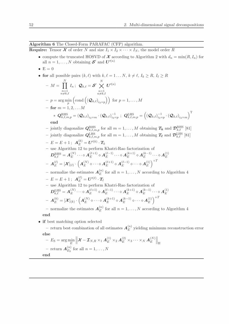
52 2. Multi-dimensional signal decompositions
Algorithm 6 The Closed-Form PARAFAC (CFP) algorithm.
Require: Tensor X of order N and size I1 × I2 × · · ·× IN , the model order R
• compute the truncated HOSVD of X according to Algorithm 2 with dn = min(R, In) forall n = 1, . . . , N obtaining S′ and U ′(n)
• E = 0
• for all possible pairs (k, ℓ) with k, ℓ = 1 . . . N , k = ℓ, Ik ≥ R, Iℓ ≥ R
– M =N∏
n=1n =k,ℓ
In ; Qk,ℓ = S′N×
n=1n =k,ℓ
U ′(n)
– p = argminp
(cond
((Qk,ℓ)i3=p
))for p = 1, . . . ,M
– for m = 1, 2, . . . M
∗ QRHSk,ℓ,m,p = (Qk,ℓ)i3=m · (Qk,ℓ)
−1i3=p ; QLHS
k,ℓ,m,p =((Qk,ℓ)
−1i3=p · (Qk,ℓ)i3=m
)T
end
– jointly diagonalize QRHSk,ℓ,m,p for all m = 1, . . . ,M obtaining Tk and DRHS
k,ℓ [81]
– jointly diagonalize QLHSk,ℓ,m,p for all m = 1, . . . ,M obtaining Tℓ and DLHS
k,ℓ [81]
– E = E + 1 ; A(k)E = U ′(k) · Tk
– use Algorithm 12 to perform Khatri-Rao factorization of
DRHSk,ℓ = A
(N)E · · · ⋄A(ℓ+1)
E ⋄A(ℓ−1)E · · · ⋄A(k+1)
E ⋄A(k−1)E · · · ⋄A(1)
E
– A(ℓ)E = [X ](ℓ) ·
(A
(N)E ⋄ · · · ⋄A(ℓ+1)
E ⋄A(ℓ−1)E ⋄ · · · ⋄A(1)
E
)+T
– normalize the estimates A(n)E for all n = 1, . . . , N according to Algorithm 4
– E = E + 1 ; A(ℓ)E = U ′(ℓ) · Tℓ
– use Algorithm 12 to perform Khatri-Rao factorization of
DLHSk,ℓ = A
(N)E · · · ⋄A(ℓ+1)
E ⋄A(ℓ−1)E · · · ⋄A(k+1)
E ⋄A(k−1)E · · · ⋄A(1)
E
– A(k)E = [X ](k) ·
(A
(N)E ⋄ · · · ⋄A(k+1)
E ⋄A(k−1)E ⋄ · · · ⋄A(1)
E
)+T
– normalize the estimates A(n)E for all n = 1, . . . , N according to Algorithm 4
end
• if best matching option selected
– return best combination of all estimates A(n)E yielding minimum reconstruction error
else
– ES = argminE
∥∥∥X − IN,R ×1 A(1)E ×2 A
(2)E ×3 · · ·×N A
(N)E
∥∥∥H
– return A(n)ES
for all n = 1, . . . , N
end

2.3. The Parallel Factor (PARAFAC) decomposition 53
2.3.3.3. The ProKRaft PARAFAC algorithm for dual-symmetric tensors
As already introduced in Section 2.3.2.5, a dual-symmetric tensor is characterized by the fact that
its PARAFAC loading matrices can be divided in two equal sets of loading matrices. Therefore,
there exists an index permutation of the dual-symmetric tensor X such that its PARAFAC
decomposition reads as
X = I2ND,R ×1 A(1) · · ·×ND A(ND) ×ND+1 A
(1)∗ · · · ×2ND A(ND)∗ , (2.93)
where the number 2ND is the order and R is the tensor rank of X . Dual-symmetric tensors
obeying the PARAFAC structure (2.93) are of high interest for applications which exploit the
correlation between multi-channel signals, since every correlation tensor according to (2.69)
shows this kind of symmetry. The analysis of correlation tensors is, e.g., a key aspect for
analytical channel models in MIMO systems [71]. Furthermore, an algorithm which is able
to exploit the special PARAFAC structure of dual-symmetric tensors can also be used for the
PARAFAC analysis of super-symmetric tensors such as the tensor of Higher Order Moments
(HOM) and the tensor of Higher Order Cumulants (HOC). Especially the PARAFAC analysis
of HOC tensors is of high interest for performing an ICA.
In the following, we derive the ProKRaft algorithm introduced in [15], which is based on
Procrustes estimation [175] and Kathri-Rao factorization (cf. Appendix B.7). In the sequel,
we assess the performance of the ProKRaft algorithm based on Monte-Carlo simulations and
analyze the performance of ProKRaft for the computation of the ICA.
The ProKRaft algorithm The Procrustes estimation and Khatri-Rao factorization (ProKRaft)
algorithm derived in this section, operates on a special matrix-unfolding for dual-symmetric
tensors. This unfolding can be applied to every dual-symmetric tensor, which has been permuted
in order to obey equation (2.93). For the permuted dual-symmetric tensor X ∈ CI1×I2×···×I2ND
of even order 2ND, this unfolding can be computed by dividing the vectorized tensor vec(X )
into block vectors xBk
vec (X )T =[x1,1,...,1, x2,1,...,1, · · · , xI1,1,...,1, xI1,2,...,1, · · · , xI1,I2,...,I2ND
]
=[(xB1
)T,(xB2
)T, · · · ,
(xBK
)T],
(2.94)
with the number K = I1 · I2 · · · · IND and k = 1, . . . ,K. Thereby, every block vector is of size
K × 1. The Hermitian-symmetric matrix unfolding XH of size K ×K can now be constructed

54 2. Multi-dimensional signal decompositions
by rearranging the block vectors xBk into the columns of the matrix
XH =[xB1 ,x
B2 , . . . ,x
BK
]. (2.95)
Therefore, the matrix XH is simply given by reshaping the tensor elements of X to a matrix of
size K ×K. Thereby, the indices of the tensor elements vary in increasing order of dimensions.
Please recognize that the unfolding (2.95) is equal to the Hermitian-unfolding in [90] apart
from the ordering of the elements. For dual-symmetric tensors according to equation (2.93) the
unfolding matrix XH is connected to the n-mode PARAFAC loading matrices by
XH =(A(ND) ⋄ · · · ⋄A(1)
)·(A(ND) ⋄ · · · ⋄A(1)
)H. (2.96)
From this equation, we can conclude that the Hermitian-symmetric matrix unfolding XH is a
positive semi-definite matrix with rank R, where R is the tensor rank of X , i.e.,
rank (X ) = rank (XH) = R . (2.97)
As a consequence of property (2.97) we can define the square root factor matrix X12H ∈ CK×R
such that
XH = X12H ·
(X
12H
)H
. (2.98)
The main idea of the ProKRaft algorithm is to construct an iterative Alternating Least Squares
(ALS) procedure in order to identify the square root factor matrix X12H and therewith all
PARAFAC n-mode loading matrices A(n). Please notice that by operating on the ”square
root factor” the amount of data involved in the algorithm is significantly reduced, namely from
K ×K scalar elements in the original tensor X to K ×R elements in the matrix X12H . Thereby,
the tensor rank R is usually much smaller than K = I1 · I2 · · · · IND . Therefore, the ProKraft
algorithm operates computationally very efficient and is able to exploit the special PARAFAC
structure (2.93) of dual-symmetric tensors.
Every square root factor matrix X12H of size K ×R and rank R according to (2.98) has to obey
the structure
X12H = UR ·ΣR ·WH , (2.99)
with UR ∈ CK×R, ΣR ∈ RR×R, and W ∈ CR×R, respectively. Here, the matrices UR and ΣR
are determined from the SVD
XH = U · S · V H , (2.100)
with U = [u1,u2, . . . ,uK ] and S = diag(σ1,σ2, . . . ,σK). The matrix UR is constructed by

2.3. The Parallel Factor (PARAFAC) decomposition 55
collecting the first R left singular vectors of XH and ΣR is a diagonal matrix containing the
square roots of the R dominant singular values of XH
UR = [u1,u2, . . . ,uR] ,
ΣR = diag (√σ1,√σ2, . . . ,
√σR) .
(2.101)
The matrix W in (2.99) represents a unitary rotation factor, which has to be determined such
that the square root factor matrix X12H follows the Khatri-Rao structure according to (2.96).
This can be achieved by comparing equations (2.96) and (2.99) yielding the main ALS equation
for the ProKRaft algorithm
UR ·ΣR ·WH =(A(ND) ⋄A(ND−1) · · · ⋄A(1)
). (2.102)
On the basis of this equation, we can design the following two least squares estimation steps,
which have to be performed in alternating iterations in order to determine the unknown param-
eters A(n) and W .
Step 1: Under the assumption that we obtained a known estimate for the rotation factor W
in (2.102) we can determine the unknown loading matrices A(n) for n = 1, . . . , ND
directly by performing aND-dimensional Khatri-Rao Factorization (KRF) on the matrix
UR ·ΣR ·WH using Algorithm 12 (cf. Appendix B.7).
Step 2: Under the assumption that we obtained known estimates for the loading matrices A(n)
for n = 1, . . . , ND, the least squares estimation of the unknown rotation factor W can be
obtained from equation (2.102) by applying the generalized solution to the Orthogonal
Procrustes Problem (OPP) [175].
For the first estimation step we assume the rotation factor W to be known in equation (2.102).
In this case we can obtain the least squares estimates for all loading matrices A(n) with
n = 1, . . . , ND by performing a ND-dimensional Khatri-Rao Factorization (KRF). An effi-
cient algorithm for performing the ND-dimensional KRF was introduced in [15] and is derived
in Appendix B.7. The necessary computational steps for computing the ND-dimensional KRF
are summarized in Algorithm 12.
For the second estimation step we assume all n-mode loading matrices A(n) to be known in equa-
tion (2.102). Then, the least squares estimate of the unknown rotation factor W is recognized
to be a Orthogonal Procrustes Problem (OPP), whose general solution has been introduced by
P. H. Schoenemann in 1966 [175]. The task of the OPP is to determine a unitary transformation
matrix W which transforms a given matrix F into a given matrix G such that FWH = G.

56 2. Multi-dimensional signal decompositions
This is achieved by minimizing the Frobenius norm of the residuals, i.e.,
minW∥F ·WH −G∥F s.t. WWH = I . (2.103)
As derived in [175], the OPP can be solved very efficiently on the basis of the SVD of the matrix
GH · F = UOPPSOPPVHOPP leading to the solution of (2.103)
W = UOPP · V HOPP . (2.104)
For the application of solution (2.104) to the second ALS estimation step based on equa-
tion (2.102) we recognize the matrices
F = UR ·ΣR ,
G =(A(ND) ⋄A(ND−1) · · · ⋄A(1)
).
(2.105)
In order to carry out the second ALS iteration step, we have to compute the SVD of the matrix
(A(ND) ⋄A(ND−1) · · · ⋄A(1)
)H·UR ·ΣR = UOPPSOPPV
HOPP , (2.106)
such that the least squares estimate of the unknown rotation factor W is given by (2.104).
By alternating the latter two estimation steps over multiple iterations we can solve the dual-
symmetric PARAFAC problem (2.93). All necessary computational steps are summarized in
Algorithm 7. The ProKRaft algorithm converges monotonically with respect to the square root
factor X12H of the data in X (however, not necessarily with respect to the data itself). The
computational complexity of one ProKRaft iteration equals the complexity of R HOSVDs for
the KRF plus the complexity of one additional matrix SVD according to (2.106). This low
computational effort per ALS iteration ensures the fast computational speed of the ProKRaft
Algorithm 7. Please notice also that in contrast to many semi-algebraic algorithms, the identi-
fiability limit (i.e., the maximum value of tensor rank R) of the ProKRaft algorithm is given by
K = I1 · I2 · · · · IND .
Performance assessment based on Monte-Carlo simulations In order to assess the perfor-
mance of the ProKRaft algorithm, we perform Monte-Carlo simulations by randomly choosing
different dual-symmetric signal tensors X ∈ RI1×I2×···×I2ND of order 2ND in every simulation
run. This is achieved by drawing the n-mode loading matrices A(n) for n = 1, . . . , ND ran-
domly from a zero mean, real-valued, unit variance, Gaussian distribution (cf. equation (2.93)).

2.3. The Parallel Factor (PARAFAC) decomposition 57
Algorithm 7 PARAFAC for dual-symmetric tensors using the Procrustes estimation andKhatri-Rao factorization (ProKRaft) algorithm.
Require: Tensor X of even order 2ND and model order REnsure: X is dual-symmetric and permuted such that
X = I2ND,R ×1 A(1) ×2 · · ·×ND A(ND) ×ND+1 A
(1)∗ ×ND+2 · · · ×2ND A(ND)∗
• reshape the vector vec(X ) =
⎡
⎢⎢⎢⎣
xB1
xB2...
xBK
⎤
⎥⎥⎥⎦with K = I1 · I2 · . . . · IND to the matrix
XH =[xB1 ,x
B2 , . . . ,x
BK
]∈ CK×K
• determine the SVD of XH = U · S · V T
• create the matrix of R dominant left singular vectors UR = [u1,u2, . . . ,uR]
• create the diagonal matrix ΣR = diag{√
s1,1,√s2,2, . . . ,
√sR,R
}containing the square
roots of the dominant R singular values of XH
• W = IR
• repeat
– use Algorithm 12 to perform Khatri-Rao factorization of
UR ·ΣR · W =(A(ND) ⋄ A(ND−1) ⋄ · · · ⋄ A(1)
)
– determine the SVD of(A(ND) ⋄ A(ND−1) ⋄ · · · ⋄ A(1)
)H·URΣR = UOPP ·SOPP ·V T
OPP
– W = UOPP · V TOPP
– erec =
∥∥∥X − I2ND,R ×1 A(1) · · · ×ND A(ND) ×ND+1 A
(1)∗ · · ·×2ND A(ND)∗∥∥∥H
∥X ∥Huntil erec stops decreasing
• return A(1), A(2), . . . , A(ND)
Furthermore, we randomly choose a noise tensor E of the same size as X from a zero mean,
real-valued, Gaussian distribution such that a predefined Signal-to-noise Ratio (SNR) according
to
SNR = 10 · log10∥X ∥2H∥E∥2H
(2.107)
is achieved. Since the estimation error of dual-symmetric tensors, such as the correlation ten-
sor (2.69) and the HOC tensor (2.72) shows always the same kind of symmetry, we choose
the symmetry of E to always correspond with the symmetry of X . For the comparison of the
different PARAFAC algorithms we decompose the noisy tensor
XN = X + E (2.108)

58 2. Multi-dimensional signal decompositions
obtaining the estimates of the n-mode loading matrices A(n). In the sequel, we can quantify the
performance of the different PARAFAC algorithms based on the relative reconstruction error
ER =∥X − I2ND,R ×1 A
(1) · · · ×ND A(ND) ×ND+1 A(1)∗ · · ·×2ND A(ND)∗∥H
∥X ∥H. (2.109)
For an adequate performance comparison based on Monte-Carlo simulations, we compare ProKRaft
against most recent PARAFAC algorithms, namely the Closed-Form PARAFAC (CFP) algo-
rithm [163] (cf. Section 2.3.3.2) and the Alternating Least Squares (ALS) PARAFAC algorithm
from the N -way toolbox version 3.10 [25] including enhanced line-search improvements [158].
Thereby, the CFP algorithm has been adapted in order to exploit the symmetry of the investi-
gated tensors (2.108). These adaptions include the usage of the Joint Diagonalization by Jacobi
Transformations (JDJT) algorithm [88] for the Joint Matrix Diagonalization (JMD), as well as a
significant reduction in the number of JMDs which have to be solved [165]. The adaption of the
CFP algorithm to symmetric tensors is presented in Appendix E.1 for the case of dual-symmetric
tensors and in Appendix E.2 for the case of super-symmetric tensors. The computational steps
for these adapted CFP algorithms are summarized in the Algorithms 13 and 14.
As a representative performance assessment, we investigate 4-th order dual-symmetric tensors
XN of size 10 × 12 × 10 × 12 with model orders (i.e., the tensor rank of X ) in the range of
R = 2, 3, . . . , 9. A typical scenario is presented in Figure 2.16(a) for a model order of R = 8 and
a SNR of 30 dB. Here, we depict the Complementary Cumulative Density Function (CCDF) of
the reconstruction error (2.109) for the three above mentioned PARAFAC algorithms ProKRaft,
CFP using JDJT, and the PARAFAC N -way toolbox algorithm. The CCDFs have been esti-
mated over 10.000 Monte-Carlo iterations and are plotted on a double-logarithmic scale in order
visualize the probability of outliers, i.e., Monte-Carlo runs on which the PARAFAC algorithms
did not fully converge. Clearly, the ProKRaft Algorithm 7 outperforms the other approaches
and it does not suffer from any outliers. In order to investigate the performance of the algorithms
also for other model orders, we compare the above mentioned techniques on the 99-percentile
highlighted by the thick, horizontal, dashed line in Figure 2.16(a). Thereby, the 99-percentile
represents the value of the reconstruction error E99%R , for which the probability of ER ≤ E99%
R
equals 99%. This 99-percentile is plotted over the model orders R = 2, 3, . . . , 9 in Figure 2.17(a).
Here, we can conclude that the ProKRaft algorithm outperforms the other approaches especially
for medium to high model orders. Furthermore, we can see that the performance of ProKRaft is
almost independent of R. Please notice that this property of ProKRaft can be interesting for the
Model Order Selection (MOS) on dual-symmetric tensors. This is because MOS techniques (cf.
Section 2.3.4) tend to reject high model orders, if the performance of the underlying PARAFAC

2.3. The Parallel Factor (PARAFAC) decomposition 59
10−3 10−2 10−1 10010−4
10−3
10−2
10−1
100
ProKRaftPARAFAC N -wayCFP via JDJT
CCDF
reconstruction error
(a) The CCDF of the reconstruction error (2.109) ona double-logarithmic scale for dual-symmetric 4-thorder tensors X of size 10 × 12 × 10 × 12 and modelorder R = 8. The CCDF is estimated on the basis of10.000 Monte-Carlo runs. The dashed horizontal linelabels the 99-percentile of the reconstruction error (cf.Figure 2.17(a)).
10−3 10−2 10−1 10010−4
10−3
10−2
10−1
100
ProKRaftPARAFAC N -wayCFP via JDJT
CCDF
reconstruction error
(b) The CCDF of the reconstruction error (2.109) ona double-logarithmic scale for super-symmetric 4-th order tensors X of size 10×10×10×10 and modelorder R = 8. The CCDF is estimated on the basis of10000 Monte-Carlo runs. The dashed horizontal linelabels the 99-percentile of the reconstruction error (cf.Figure 2.17(b)).
Figure 2.16.: The performance of the ProKRaft algorithm in comparison to the CFP using JDJT(cf. Appendix E), and the PARAFAC N -way algorithm from the N -way toolbox 3.10 [25].
algorithms is getting worse for high values of R. A similar performance behavior was observed
for SNR values of 50 dB and 70 dB. In the very low SNR region all algorithms show a comparable
performance.
For the cumulant based computation of the ICA it is of high interest to efficiently diagonalize the
tensor of Higher Order Cumulants (HOC) using a PARAFAC procedure (cf. Section 2.3.3.3).
Since HOC tensors are always super-symmetric in the real-valued case, we test the performance
of the ProKRaft Algorithm 7 also for the case of a 4-th order super-symmetric tensor XN of
size 10 × 10 × 10 × 10. In analogy to the above presented simulation setup for dual-symmetric
tensors, we depict the resulting CCDF of the reconstruction error (2.109) in Figure 2.16(b) for a
representative model order of R = 8. We can conclude that the ProKRaft algorithm outperforms
the other PARAFAC methods especially in the super-symmetric case. Please notice that the
special case of super-symmetry can be exploited by the ProKRaft algorithm by simplifying
the Khatri-Rao Factorization (KRF) step (2.102) in Algorithm 7 (cf. Appendix B.7). For the
performance comparison over varying model orders R, we present the 99-percentile E99%R of the
reconstruction error for all above mentioned PARAFAC methods in Figure 2.17(b). Similar to
the results for dual-symmetric tensors, we can observe that the ProKRAft algorithm outperforms
the other approaches especially for medium to high values of the model order R. Again, the
performance of ProKRaft is almost independent of R.

60 2. Multi-dimensional signal decompositions
2 3 4 5 6 7 8 90
0.005
0.01
0.015
ProKRaftPARAFAC N -wayCFP via JDJT
99-percentile
model order
(a) The 99-percentile E99%R of the reconstruction er-
ror (2.109) for dual-symmetric 4-th order tensors ofsize 10 × 12 × 10 × 12 over varying model orders R.The 99-percentile was estimated on the basis of 10.000Monte-Carlo iterations (cf. Figure 2.16(a)).
2 3 4 5 6 7 8 90
0.01
0.02
0.03
0.04
ProKRaftPARAFAC N -wayCFP via JDJT
99-percentile
model order
(b) The 99-percentile E99%R of the reconstruction er-
ror (2.109) for super-symmetric 4-th order tensorsof size 10 × 10 × 10 × 10 over varying model ordersR. The 99-percentile was estimated on the basis of10.000 Monte-Carlo iterations (cf. Figure 2.16(b)).
Figure 2.17.: The performance of the ProKRaft algorithm in comparison to the CFP using JDJT(cf. Appendix E), and the PARAFAC N -way algorithm from the N -way toolbox 3.10 [25].
In order to compare the computational effort for the different PARAFAC algorithms on dual-
symmetric and super-symmetric tensors, we present distributional parameters for the computa-
tional time per run estimated over 10.000 realizations in Table 2.4. The simulation parameters
are the same as in the previously discussed scenarios presented in Figure 2.16. Based on these
results we can conclude that the ProKRaft algorithm performs significantly faster than the other
approaches for both symmetry cases. This indicates that the ALS iteration procedure presented
in Algorithm 7 converges usually very fast. Please note that it is not suitable to compare
the distributional parameters of the computation time between the super-symmetric and the
dual-symmetric case, since these simulations were carried out on different machines.
Application for the computation of the independent component analysis (ICA) The ICA is
one of the most successfully applied Blind Source Separation (BSS) techniques, which has been
used in a variety of signal and image processing fields such as communication systems, audio
signal processing, biomedical signal processing, analysis of financial data and much more. For a
comprehensive introduction to ICA algorithms and applications we refer to [55,109,111]. In the
field of biomedical signal processing, the ICA has proven to be very useful for the separation
of artifacts and technical distortions from desired components of multi-channel signals, such as
MagnetoEncephaloGram (MEG) or ElectroEncephaloGram (EEG) [72,74,120]. The ICA is also
investigated throughout this thesis as the standard two-dimensional (2D) signal decomposition

2.3. The Parallel Factor (PARAFAC) decomposition 61
Symmetry ProKRaft PARAFAC N-way CFP Distributional parameter
dual-symmetric38 ms 58 ms 82 ms median41 ms 65 ms 85 ms mean15 ms 30 ms 26 ms STD
super-symmetric138 ms 289 ms 218 ms median223 ms 456 ms 315 ms mean326 ms 577 ms 400 ms STD
Table 2.4.: Comparison in computation time for the different PARAFAC algorithms on dual-symmetric and super-symmetric tensors. The median, the mean-value and the STandarddeviation (STD) of the computational time where estimated over 10.000 simulation runs.
strategy for EEG data. In this context, the ICA is used as the well established reference
decomposition strategy in order to judge the performance of the multi-dimensional tensor based
decompositions discussed in Chapter 3 and 4.
The ICA is based on a linear mixing model, which creates a linear superposition of R source
signals xr(t) resulting in a set of M sensor signals ym(t). In matrix-vector notation this is
represented by
y(t) = A · x(t) , (2.110)
with the vector of sensor signals y(t) = [y1(t), . . . , yM (t)] ∈ RM and the vector of source signals
x(t) = [x1(t), . . . , xR(t)] ∈ RR. The mixing matrix A is of size M × R and assumed to be
unknown in the context of BSS. Therefore, the general BSS task is to identify the source signals
x(t) from (2.110) without the knowledge of the mixing matrix A, i.e., only from the observation
of the sensor signals y(t). In general this task can only be achieved by introducing additional
assumptions on the source signals x(t). In case of the ICA, these assumptions are
• the source signals xr(t) are mutually statistically independent;
• the Probability Density Function (PDF) of the source signals is not Gaussian;
• the source signals xr(t) are ergodic and therefore also stationary.
In the following, we also assume that all source signals x(t) and therewith the sensor signals
y(t) are centered, i.e., E(x(t)) = 0. Furthermore, we assume unit variance on xr(t) for all
r = 1, . . . , R, since the scaling ambiguity inherent to the BSS problem (2.110) inhibits an unique
determination of the variances of the sources. From both assumptions we can conclude without
loss of generality that
E(x(t) · x(t)T
)= I . (2.111)
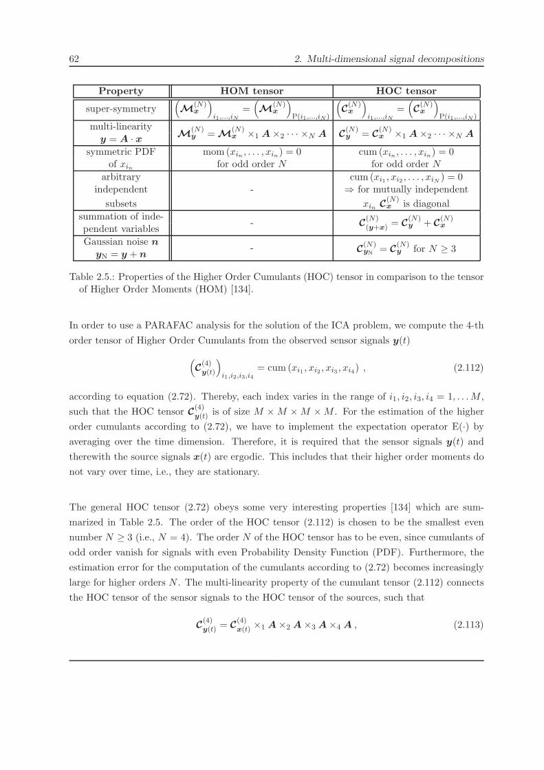
62 2. Multi-dimensional signal decompositions
Property HOM tensor HOC tensor
super-symmetry(M
(N)x
)
i1,...,iN=
(M
(N)x
)
P(i1,...,iN )
(C(N)x
)
i1,...,iN=
(C(N)x
)
P(i1,...,iN )
multi-linearityM
(N)y = M
(N)x ×1 A×2 · · · ×N A C
(N)y = C
(N)x ×1 A×2 · · · ×N A
y = A · xsymmetric PDF mom (xin , . . . , xin) = 0 cum (xin , . . . , xin) = 0
of xin for odd order N for odd order Narbitrary
-cum (xi1 , xi2 , . . . , xiN ) = 0
independent ⇒ for mutually independent
subsets xin C(N)x is diagonal
summation of inde-- C
(N)(y+x) = C
(N)y + C
(N)xpendent variables
Gaussian noise n- C
(N)yN = C
(N)y for N ≥ 3
yN = y + n
Table 2.5.: Properties of the Higher Order Cumulants (HOC) tensor in comparison to the tensorof Higher Order Moments (HOM) [134].
In order to use a PARAFAC analysis for the solution of the ICA problem, we compute the 4-th
order tensor of Higher Order Cumulants from the observed sensor signals y(t)
(C(4)y(t)
)
i1,i2,i3,i4= cum (xi1 , xi2 , xi3 , xi4) , (2.112)
according to equation (2.72). Thereby, each index varies in the range of i1, i2, i3, i4 = 1, . . .M ,
such that the HOC tensor C(4)y(t) is of size M ×M ×M ×M . For the estimation of the higher
order cumulants according to (2.72), we have to implement the expectation operator E(·) by
averaging over the time dimension. Therefore, it is required that the sensor signals y(t) and
therewith the source signals x(t) are ergodic. This includes that their higher order moments do
not vary over time, i.e., they are stationary.
The general HOC tensor (2.72) obeys some very interesting properties [134] which are sum-
marized in Table 2.5. The order of the HOC tensor (2.112) is chosen to be the smallest even
number N ≥ 3 (i.e., N = 4). The order N of the HOC tensor has to be even, since cumulants of
odd order vanish for signals with even Probability Density Function (PDF). Furthermore, the
estimation error for the computation of the cumulants according to (2.72) becomes increasingly
large for higher orders N . The multi-linearity property of the cumulant tensor (2.112) connects
the HOC tensor of the sensor signals to the HOC tensor of the sources, such that
C(4)y(t) = C
(4)x(t) ×1 A×2 A×3 A×4 A , (2.113)

2.3. The Parallel Factor (PARAFAC) decomposition 63
because of the linear mixing model (2.110). Furthermore, higher order cumulants with orders
N ≥ 3 vanish if any two subsets of the analyzed signals become statistically independent.
Therefore, the ICA assumption of mutually statistically independent source signals x(t) leads
to a diagonal HOC tensor C(4)x in (2.113) [69]. With the normalization of the source signals
according to (2.111), we can conclude that the HOC tensor of the sources C(4)x(t) equals a fourth-
order identity tensor, such that
C(4)y(t) = I4,R ×1 A×2 A×3 A×4 A . (2.114)
At this point it is easily recognized that the ICA problem can be solved by performing a
PARAFAC analysis on the super-symmetric tensor C(4)y(t) according to equation (2.114). Thereby,
the connection between the ICA and the super-symmetric PARAFAC is a direct corollary of
the properties of the HOC tensor (cf. Table 2.5). With a known number of source signals R,
the PARAFAC problem (2.114) can be solved using the ProKRaft Algorithm 7 leading to an
estimate of the mixing matrix A. Once this estimate is computed, we can determine the source
signals x(t) by
x(t) = A+ · y(t) , (2.115)
where A+ denotes the Moore-Penrose pseudo-inverse of the estimated mixing matrix A [192].
The general method of computing the ICA by solving the super-symmetric PARAFAC prob-
lem (2.114) offers some very nice theoretical properties. First, the method is not affected by
Gaussian noise, since the HOC tensor C(4)y(t) is invariant with respect to additive Gaussian noise
which is statistically independent from the sensor signals y(t) (cf. the last properties of the HOC
tensor presented in Table 2.5). Second, the method does not include any a-priori assumptions on
the source signals, which influence the derivation of (2.113) (only the linear mixing model (2.110)
has to be valid). As a consequence, the method can be applied also if the source signals are
not statistically independent. In this case it is possible to identify source signals, which are
”as independent as possible” by approximately solving equation (2.113) in the sense that the
cumulant tensor of the sources is getting ”as diagonal as possible” [57]. A simulation example
where the source signals are not independent is given in Figure 4.14 (Section 4.2.1.2). Here,
the diagonalization of the 4-th order HOC tensor using ProKRaft leads to the best performance
among all considered ICA algorithms. Unfortunately, the main practical drawback of solving
the ICA problem using the ProKRaft algorithm on (2.114) is the estimation of the 4-th order
cumulant tensor C(4)y(t). The estimation of this HOC tensor according to (2.72) usually requires
a high number of temporal snapshots in order to keep the estimation error within acceptable
bounds. This estimation error is also the reason why the above mentioned noise properties are

64 2. Multi-dimensional signal decompositions
not completely fulfilled in practice. One possibility to reduce the estimation error of the HOC
tensor is to perform a pre-whitening on the sensor signals y(t) using
z(t) = Σ− 12UT · y(t) with E
(y(t)y(t)T
)= UΣUT . (2.116)
In the sequel, we can compute the HOC tensor C(4)z(t) ∈ RR×R×R×R of the uncorrelated signal
z(t) using the simplified equation
C(4)z(t) = E(xi1xi2xi3xi4)− (I2,R)i1,i2 · (I2,R)i3,i4 − (I2,R)i1,i3 · (I2,R)i2,i4
− (I2,R)i1,i4 · (I2,R)i2,i3 with i1, i2, i3, i4 = 1, . . . , R ,(2.117)
which only involves the estimation of one 4-th order moment. After the pre-whitening, we can
solve the ICA problem by running the ProKRaft algorithm on the HOC tensor C(4)z(t), thus solving
the super-symmetric PARAFAC problem
C(4)z(t) = I4,R ×1 V
T ×2 VT ×3 V
T ×4 VT , (2.118)
where the matrix V ∈ RR×R is the matrix of right singular values of the mixing matrix A,
i.e., A = UΣ12V T. By introducing the pre-whitening, we obtain the advantage of reducing the
estimation error of the HOC tensor of the sensor signals, and therefore boosting the performance
of the ICA algorithm. However, we loose the possibility of computing the ICA also in under-
determined cases where the number of sources exceeds the number of sensors. Furthermore, the
pre-whitening introduces the a-priori assumption that the sensor signals are at least uncorrelated.
The computational steps for solving the ICA problem by diagonalizing the HOC tensor (2.114)
using ProKRaft are summarized in Algorithm 8. This algorithm also includes the option of
performing a pre-whitening. In order to demonstrate the performance of Algorithm 8 we com-
pare it to the JADE [44, 46] algorithm as well as the FastICA algorithm [110, 111]. Here, we
choose the JADE algorithm because it is structurally very similar to the proposed Algorithm 8
in the sense that it is also based on the diagonalization of the HOC tensor (2.113). On the
other side, the kurtosis (i.e., fourth order cumulant) based FastICA algorithm is one of the most
popular algorithms for solving the ICA problem. In order to compare these three algorithms we
again perform Monte-Carlo simulations by randomly drawing independent uniformly distributed
source signals x(t). Furthermore, the mixing matrix is drawn randomly from a normal distri-
bution on each run. For an objective comparison measure, we use the relative estimation error
erel by computing the relative distance between the exact mixing matrix A and the estimated

2.3. The Parallel Factor (PARAFAC) decomposition 65
Algorithm 8 The ICA algorithm based on the PARAFAC analysis of the super-symmetriccumulant tensor using ProKRaft. The algorithm is able to run with or without pre-whitening.
Require: Sensor signals y ∈ RM number of sources R.
• if pre-whitening option selected
– Ryy = E(y · yT
); Ryy = UΣUT
– UR = [u1,u2, . . . ,uR]; ΣR = diag (σ1,σ2, . . . ,σR)
– P = Σ− 1
2R ·UT
R ; yP = P · y
– for i1 = 1, . . . , R; for i2 = 1, . . . , R; for i3 = 1, . . . , R; for i4 = 1, . . . , R
∗
(C(4)yP
)
i1,i2,i3,i4= E
(yPi1 · y
Pi2 · y
Pi3 · y
Pi4
)− (I2,R)i1,i2 · (I2,R)i3,i4 − (I2,R)i1,i3 ·
(I2,R)i2,i4 − (I2,R)i1,i4 · (I2,R)i2,i3end; end; end; end
– solve the super-symmetric PARAFAC problem C(4)yP = I4,R ×1 B ×2 B ×3 B ×4 B
by using the ProKRaft Algorithm 7 obtaining an estimate of B.
– A = PT ·Belse
– for i1 = 1, . . . ,M ; for i2 = 1, . . . ,M ; for i3 = 1, . . . ,M ; for i4 = 1, . . . ,M
∗
(C(4)y
)
i1,i2,i3,i4= cum (yi1 , yi2 , yi3 , yi4) according to (2.72)
end; end; end; end
– solve the super-symmetric PARAFAC problem C(4)y = I4,R ×1 A ×2 A ×3 A ×4 A
by using the ProKRaft Algorithm 7 obtaining an estimate of A.
end
• x = A+y
• return source signals x
• return mixing matrix A
mixing matrices A
erel =∥A− A∥F∥A∥F
. (2.119)
Thereby, the different permutation and scaling ambiguities between the exact mixing matrix A
and the estimated mixing matrices A are resolved automatically.
In Figure 2.18, we present the Complementary Cumulative Density Function (CCDF) of the
relative estimation error (2.119) estimated over 10.000 realizations [15]. The number of sources
R and the number of sensor signals M where chosen to be equal to ten, such that M = R = 10.
Please recognize that all algorithms perform their computations on the pre-whitened signals.
From these simulations we can conclude that the ProKRaft based ICA Algorithm 8 outperforms

66 2. Multi-dimensional signal decompositions
10−3 10−210−4
10−3
10−2
10−1
100
ProKRaftJADEFastICA
relative sum of square error of A
CCDF
Figure 2.18.: The CCDF of the relative estimation error (2.119) of the mixing matrix A fordifferent ICA algorithms. The CCDF is plotted on a double-logarithmic scale and estimatedover 10.000 simulation runs.
the FastICA approach and performs equally well as the JADE algorithm. In contrast to JADE
or FastICA, the ProKRaft based ICA algorithm is able to determine the mixing matrix A also
in the under-determined case from equation (2.114) if no pre-whitening is applied.
2.3.4. Model order selection for the PARAFAC model
For the application of PARAFAC to practical scenarios it is crucial to identify the tensor rank
R of the desired signal tensor X . However, in almost all applications the signal tensor X is
contaminated by additive noise E such that the observed measurement tensor XN is given by
(cf. Section 2.3.3)
XN = X + E . (2.120)
Here, the typical rank of the measurement tensor XN ∈ CI1×I2×···×IN usually reaches very high
values [59] and is not connected to the tensor rank of X , which is also termed the model order of
the tensor XN. In order to determine the model order R, let us assume a certain candidate model
order P . With this candidate model order we can determine the PARAFAC approximation
XN ≈ IN,P ×1 A(1) ×2 A
(2) ×3 · · ·×N A(N) , (2.121)
using, e.g., an ALS based algorithm (cf. Section 2.3.3.1). After the computation of the loading
matrices A(n) for n = 1, . . . , N using ALS, we can reformulate equation (2.121) to the equivalent

2.3. The Parallel Factor (PARAFAC) decomposition 67
matrix version (cf. Section A.7)
[XN](1) ≈ A(1) ·CP ·(A(N) ⊗A(N−1) ⊗ · · ·⊗A(2)
)T, (2.122)
where the matrix CP is of size I1 × I2 · I3 · · · · IN . Please notice that the choice of the one-
mode unfolding in (2.122) is arbitrary, however it simplifies the following equations. Under the
theoretical assumptions that there is no noise (i.e., the model order R equals the tensor rank
of XN) and that the candidate model order P is equal to the model order R, equation (2.122)
becomes an exact equality and we can conclude that the core matrix CR is given by the one-
mode unfolding of the identity tensor IN,R, i.e., CR = [IN,R](1) (cf. Appendix A.7). The main
assumption of the CORe CONsistancy DIAgnostics (CORCONDIA) [42] is that in presence of
noise the matrix CP is closest to the unfolding of the identity tensor IN,R, if the candidate
model order P is smaller or equal to the model order R. The CORCONDIA is one of the most
prominent Model Order Selection (MOS) techniques for the PARAFAC decomposition and is
used in a variety of applications [60]. In order to estimate the model order R via CORCONDIA,
we calculate the PARAFAC approximation (2.121) using an ALS procedure for every value
within a predefined range of the candidate model orders P . In the sequel, we can estimate the
core matrix CP from equation (2.122) by utilizing the properties of the Kronecker product and
the vec{·} operator [38,155] leading to
vec (CP ) =(A(N) ⊗A(N−1) ⊗ · · ·⊗A(1)
)+· vec (XN) . (2.123)
Consecutively, the core consistency is given as the following measure of similarity between the
core matrix CP and the one-mode unfolding of the identity tensor
eCC(P ) = 100 ·
⎛
⎜⎝1−
∥∥∥CP − [IN,P ](1)
∥∥∥2
F
∥CP ∥2F
⎞
⎟⎠ . (2.124)
According to [42] it is proposed to identify the model order R by a subjective assessment of
the core consistency profile (2.124). Thereby, R can be determined at the position of an abrupt
descent in eCC(P ). An exemplary profile for a tensor of order 3 and model order 5 is depicted
in Figure 2.19. The size of this tensor is selected to the typical values 21× 64× 32 of the EEG
processing applications discussed in Chapter 4. Please notice that the hight of the descent in
the profile at the exact model order of 5 depends not only on the SNR and the size of the tensor,
but also on the actual noise realization. Therefore, a subjective analysis of the profile eCC(P )
is necessary. One of the main advantages of the CORCONDIA model order selection technique

68 2. Multi-dimensional signal decompositions
1 2 3 4 5 6 7 80
20
40
60
80
100
0 dB10 dB20 dB
e CC(P
)
candidate model order P
Figure 2.19.: The core consistency profile eCC(P ) for a tensor of order 3 and size 21 × 64 × 32.The model order was chosen to 5. A clear and abrupt descent in the consistency profile isrecognized at a candidate model order of P = 5 for all SNR values. In this scenario however,the magnitude of this descent shows a stronger dependence to the actual noise realization thanto the SNR. Therefore, the determination of a fixed threshold is difficult and a subjectiveanalysis has to be performed.
is that it does not impose any assumptions on the noise distribution and its spatial correlation.
Furthermore, the maximum value for the candidate model order is only restricted by the typical
rank of XN. On the other side CORCONDIA shows a high computational complexity, since
the PARAFAC approximation (2.121) has to be computed for every candidate model order P .
Additionally, the CORCONDIA technique cannot be automatized, since the final selection of
the estimated model order R is based on a subjective assessment of the core consistency profile
eCC(P ). This disadvantage of CORCONDIA can be avoided by considering the non-subjective
extension, named Threshold-CORCONDIA, which is derived and analyzed in [64,67].
For two-dimensional (2D) data a great variety of Model Order Selection (MOS) techniques can
be found in literature. The most well known reference techniques found there are the statistically
based Akaike Information Criterium (AIC) [22] and the Minimum Description Length (MDL)
method [161]. These two MOS techniques are based on the information theoretic criterium
applied to the eigenvalue profile of the sample covariance matrix of the measured data [209].
Both methods assume that the noise eigenvalues have constant magnitude. In theory, this
assumption is exactly fulfilled in case of additive, zero mean, spatially uncorrelated noise (i.e.,
the noise covariance matrix is given by σ2 ·I, with σ2 being the noise variance), where the number
of time snapshots approaches infinity. Therefore, these methods show a good performance in case
of large amounts of data. In cases where only a small number of time snapshots is available,
the noise eigenvalues of the sample covariance matrix show an exponential profile. In these

2.3. The Parallel Factor (PARAFAC) decomposition 69
situations the Exponential Fitting Test (EFT) [157] outperforms other approaches. In order to
be able to generalize these methods to the multi-dimensional case, the authors in [65] introduced
the concept of global eigenvalues, which are defined by
λGi =N∏
n=1
λ(n)i . (2.125)
Here, N is the order of the tensor XN ∈ CI1×I2×···×IN and i varies within the range i =
1, . . . ,min(I1, I2, . . . , IN ). Furthermore, λ(n)i are the eigenvalues of the n-mode sample covariance
matrix, which are connected to the higher-order singular values (cf. Section 2.2) by
λ(n)i =InIT
(σ(n)i
)2, (2.126)
where IT = I1·I2 · · ··IN . All the assumptions imposed by the AIC, MDL and EFT MOS methods
are also valid if the global eigenvalues (2.125) of the N -th order tensor XN are used [60]. The
corresponding multi-dimensional extensions of these methods are the N -D AIC, the N -D MDL
and the N -D EFT, which are derived in [64,65]. The MOS based on the generalized information
theoretic criterium reads as
R = argminP
J(P ) with
J(P ) = −NS (I − P ) ln
(ΛG(P )
λG(P )
)+ L(P,NS, I) .
(2.127)
Thereby, λG(P ) and ΛG(P ) represent the arithmetic and the geometric mean of the P smallest
global eigenvalues
λG(P ) =1
P
I∑
i=I−P+1
λGi and ΛG(P ) = P
√√√√I∏
i=I−P+1
λGi , (2.128)
with I = min(I1, I2, . . . , IN ). Furthermore, the N -D AIC and the N -D MDL differ only in the
choice of the penalty function L(P,NS, I), which is chosen as [67]
N -D AIC : L(P,NS, I) = P · (2I − P )
N -D MDL : L(P,NS, I) =1
2P · (2I − P ) · ln(NS) .
(2.129)
The parameter NS refers to the number of temporal snapshots in the classical 2D AIC and MDL
approach. For the purpose of the general MOS of a tensor XN it is proposed to choose NS as

70 2. Multi-dimensional signal decompositions
−30 −20 −10 0 10 20 300
0.2
0.4
0.6
0.8
1
Probab
ilityof
detection
SNR in dB
N -D AIC
N -D MDL
Figure 2.20.: The probability of detection over varying SNR for global eigenvalue based modelorder selection techniques. For these simulations we draw random realizations of tensors oforder 3 and size 64 × 128 × 64. We considered white gaussian, spatially uncorrelated noiseand the model order was chosen to be 4. The number of realizations is 1000 for each SNR.
the maximum over all tensor sizes, i.e., NS = max(I1, I2, . . . , IN ).
In Figure 2.20 we compare the performance of the N -D AIC, and the N -D MDL in terms of the
probability of detection achieved over 1000 trial runs for different SNR. For a detailed discussion
of the N -D EFT we refer to [67]. In this simulation, we choose an order three tensor of model
order 4 with the typical sizes 64× 128 × 64 as used in the EEG applications in Chapter 4. For
large third order tensors the performance of the N -D AIC, the N -D MDL and theN -D EFT does
not differ significantly [60]. However, the computational complexity of the N -D AIC, and the
N -D MDL is superior to the N -D EFT. Please notice that in contrast to the CORCONDIA the
letter three MOS techniques are only applicable in case of additive white Gaussian noise, which
is spatially uncorrelated. For a detailed analysis and comparison of various MOS techniques
including exhaustive simulations for both white and colored noise scenarios, we refer to [60].
For the model order selection in the case of EEG applications we draw the following conclusions.
Since the noise in EEG measurements is always spatially correlated [106] and shows an unknown
amplitude PDF, the N -D AIC, the N -D MDL and the N -D EFT are only applicable in scenarios
with high SNR, where the performance difference between the case of colored noise and white
noise is negligible. For these cases we propose to use the N -D AIC, since it provides a low
computational effort and shows the same performance as the other approaches for the typically
large tensor sizes in EEG scenarios. In cases where a high SNR cannot be achieved we have to
choose a subjective MOS technique like CORCONDIA in order to estimate the correct model
order. Furthermore, the subjective assessment of the global eigenvalue profile (2.125) as well

2.3. The Parallel Factor (PARAFAC) decomposition 71
as additional neuro-physiological knowledge specific to the performed experiments can be of
additional help for the determination of the correct model order.
2.3.5. Comparison between the PARAFAC decomposition and the HOSVD
At this point we have described two different tensor decomposition techniques for multi-way
signals X ∈ CI1×I2···×IN of order N , namely the Higher Order Singular Value Decomposi-
tion (HOSVD) and the PARAllel FACtor (PARAFAC) analysis. In order to facilitate the dis-
tinction between these two decomposition methods, we compare their structure as well as their
main properties in Table 2.6. Both tensor decompositions can be seen as different higher order
generalizations of the matrix SVD (cf. Section 2.1). Thereby, the HOSVD handles the original
tensor X as a collection of n-mode vectors, which are straight forward generalizations of the
column and row vectors of matrices. This way of analyzing a higher order tensor leads to the
concept of n-ranks, which represent the dimensions of the n-mode vector spaces. The HOSVD
analyzes the n-mode vector spaces by means of orthogonal transformations utilizing the matrix
SVD of the n-mode unfoldings (2.22). Therefore, the HOSVD loading matrices U (n) (i.e., the
matrices of higher order singular vectors) provide a unitary basis for the n-mode vector spaces
of X . The formulation of the HOSVD and PARAFAC by means of the n-mode product provides
one of the most compact possibilities to compare both decompositions (cf. the first two rows of
Table 2.6). In contrast to PARAFAC (and the matrix SVD), the core tensor S of the HOSVD
is in general a full tensor with the property of all-orthogonality (cf. Section 2.2.3.1).
In contrast to the HOSVD, the PARAFAC decompositions handles the original tensor X as a
sum of rank-one tensors. Thereby, the definition of a rank-one tensor is a direct generalization
of the definition of a rank-one matrix, i.e., a rank-one tensor can be represented by the outer
product of N vectors (cf. Section 2.1.4). Furthermore, the PARAFAC decomposition forces the
number of rank-one components (rank-one tensors) to be minimal. In this context, the minimal
number of rank-one components is termed the tensor rank R of X . In terms of the number
of components, the PARAFAC decomposition is much more compact than the HOSVD, which
extracts a total number of R1 ·R2 · · · ·RN pairwise orthogonal components. However, in contrast
to the HOSVD, different PARAFAC components can share common parts of the total energy of
X . Therefore, the PARAFAC components are not uncorrelated, such that the n-mode loading
matrices A(n) are not orthogonal. The compact representation of the tensor X delivered by the
PARAFAC analysis as well as the moderate uniqueness conditions (cf. Section 2.3.2.2) build
the foundation for the big success of PARAFAC, since it can be applied to a variety of problems
without imposing additional constraints. However, the fact that the PARAFAC components are

72 2. Multi-dimensional signal decompositions
Property HOSVD PARAFAC
n-mode structure
!"#$%&'()*+,-./0123456789:;<=>?@ABCDEFGHIJKLMNOPQRSTUVWXYZ[\]^_`abcdefghijklmnopqrstuvwxyz{|}~
= 12
3
X U(1) S U
(2)
U(3)
!"#$%&'()*+,-./0123456789:;<=>?@ABCDEFGHIJKLMNOPQRSTUVWXYZ[\]^_`abcdefghijklmnopqrstuvwxyz{|}~
= 12
3
X A(1) I3,4 A
(2)
A(3)
n-mode formulation X = S ×1 U(1) ×2 · · ·U (N) X = IN,R ×1 A
(1) ×2 · · ·A(N)
component formulationX =
R1∑
i1=1
· · ·RN∑
iN=1
si1,...,iN · U i1,...,iNX =
R∑
r=1
a(1)r ◦ · · · ◦ a(N)
r
with U i1,...,iN = u(1)i1◦ · · · ◦ u(N)
iNrank concept n-ranks Rn tensor rank R
n-mode loadingsunitary
not unitarySize In ×R
Size In × Ineconomy Size In ×Rn
core tensor
full tensorSize I1 × I2 · · · × IN diagonal tensor
economy Size R1 ×R2 · · ·×RN Size R×R · · ·×Rall-orthogonal
component weightscore tensor component amplitudes
elements si1,...,iN γr with r = 1, . . . , R
singular valuesIn higher order
/singular values σ(n)i foreach mode n = 1, . . . , N
computationalcomplexity
low highclosed-form solution semi-algebraic or
complexity of N SVDs iterative solution
Table 2.6.: Comparison of the structure and the main properties of the PARAFAC decompositionand the HOSVD.
correlated makes it difficult to evaluate the contribution of single components to the total energy
of the multi-dimensional signal X . Therefore, the interpretation of the PARAFAC components
is often more difficult compared to the HOSVD.
In terms of the computational complexity, the PARAFAC analysis is usually much worse than
the HOSVD, which can be computed closed-form by solving N matrix SVDs. The investigation
of most efficient methods for computing PARAFAC in various scenarios is still a big part of
ongoing research [162]. It has to be pointed out that the model order selection (i.e., the number
of components to be extracted) for the PARAFAC decomposition is a challenging task in many
applications. Usually PARAFAC algorithms assume that the model order is known a-priori.

2.3. The Parallel Factor (PARAFAC) decomposition 73
Finally, it has to be noted that although both the HOSVD and the PARAFAC decomposition
are direct generalizations of the matrix SVD, their properties are often different compared to
the SVD. These differences become evident in practical situations especially for the problem
of low n-rank approximations (cf. Section 2.2.3.2) in case of the HOSVD and low tensor rank
approximations (cf. Section 2.3.2.3) in case of PARAFAC.
2.3.6. Applications of the PARAFAC model
The PARAFAC analysis is often successfully applied in a variety of different scientific fields [39,
128]. Furthermore, also possibly new fields of applications are currently discovered in ongoing
research. The PARAFAC decomposition has its origins in the field of psychometrics. Here, it
was introduced by Carroll and Chang in 1970 in order to analyze similarities of the data ma-
trices obtained from different subjects [47]. In the same year Harshman introduced PARAFAC
independently from [47] and applied it to phonetic data measurements in order to analyze the
formants of spoken vowel sounds from different test persons [93].
In the field of communication the PARAFAC decomposition was proposed by J. P. C. L. da Costa,
F. Roemer, M. Weis and M. Haardt in 2010 for the parameter estimation in multi-user Multiple
Input Multiple Output (MIMO) scenarios [1]. Thereby, spatial frequencies where successfully
estimated with increased robustness for arbitrary array geometries. Furthermore, N. Sidiropou-
los et al. used PARAFAC for the design of space-time codes [183] and blind receivers in direct
sequence code division multiple access (DS-CDMA) systems [184].
PARAFAC is also widely used in the field of multi-media. In these applications the PARAFAC
model is often used together with a non-negativity constraint on the loading matrices, also
termed Non-negative Tensor Factorization (NTF). D. Fitzgerald et al. used the NTF for the
sound source separation in recorded music in order to separate musical instruments [80]. In 2001
A. Shashua et al. used PARAFAC for the sparse image coding in computer vision [179] and for
the statistical classification of image data [178]. Furthermore, A. Shashua et al. used the super-
symmetric NTF for the illumination-based clustering of human faces [180]. Also PARAFAC has
been applied in the field of video compression in order to achieve higher compression rates [208].
The PARAFAC decomposition is also applied in a number of other fields [128]. The first usage
of PARAFAC in the context of data mining was proposed by E. Acar et al. in the year 2005 [20].
Additionally, B. W. Bader et al. used PARAFAC for different text-mining applications [28], e.g.,
the analysis of online chatrooms. In the field of chemometrics, PARAFAC was introduced by
C. J. Appellof and E. R. Davidson in the year 1981 [26]. For a comprehensive overview of the
role of PARAFAC in this field we refer to [24].

74 2. Multi-dimensional signal decompositions
Very recently, PARAFAC has been introduced by T. Just et al. for the automatic clustering of
neural spikes [5]. Thereby, PARAFAC is used for the spike feature extraction, which leads to
an improved clustering performance. In the field of neuroscience, especially for the analysis of
ElectroEncephaloGram (EEG) data, PARAFAC is widely used by many authors. For a detailed
overview we refer to the state of the art on EEG processing strategies in Section 3.2. Throughout
this thesis, PARAFAC has a major role in the investigations about EEG signal decomposition
strategies, which are subject to the Chapters 3 and 4. Furthermore, PARAFAC is used in the
direct fitting algorithm for the PARAFAC2 decomposition in Section 2.4.3, as well as for the
computation of the ICA in Section 2.3.3.3.
2.4. The PARAFAC2 model
The PARAllel FACtor2 (PARAFAC2) decomposition was introduced in 1972 by Harshman [94]
as a generalization of the PARAFAC model in order to analyze cross-product matrices. Many
years later in 1999, the PARAFAC2 analysis was used by H. A. L. Kiers and R. Bro et al. for the
analysis of retention time shifts in the field of chemometrics [40, 126]. This work also inspired
the usage of PARAFAC2 for the analysis of time-frequency-space atoms in the field of EEG
signal processing in Chapter 3 and 4. The PARAFAC2 analysis can be seen as the higher order
generalization of shifted factor analysis [96, 104,105].
The PARAFAC2 decomposition is restricted to three dimensions. In its most general form
PARAFAC2 is not a tensor decomposition in strict sense. In fact, PARAFAC2 can be used for
the analysis of a stack of matrices which may have either a varying number of columns or a
varying number of rows. In Figure 2.21, we present the structure of the general PARAFAC2
model for a stack of matrices Xk where the number of rows vary with k. However, for the
application of PARAFAC2 in the field of neuroscience only the case of third order tensors has
to be considered. Therefore, we restrict the sizes of the matrix stack Xk to be constant over
k throughout the scope of this thesis. This enables us to formulate the PARAFAC2 model for
third order tensors according to Figure 2.22. The restriction of PARAFAC2 to the tensor case
greatly simplifies the mathematical notation in the following sections.
The fact that the PARAFAC2 model for tensors can be seen as a generalization of three-way
PARAFAC is easily recognized by comparing the PARAFAC representation in the last column of
Table 2.1 and the PARAFAC2 structure in Figure 2.22 used throughout this thesis. In contrast
to PARAFAC, the PARAFAC2 model supports an additional variation of one of the n-mode
loading matrices over a second dimension (cf. Section 2.4.1). This additional degree of freedom

2.4. The PARAFAC2 model 75
!"#$%&'()*+,-./0123456789:;<=>?@ABCDEFGHIJKLMNOPQRSTUVWXYZ[\]_abcdefghijklmnopqrstuvwxyz{|}~
=
Xk Ak diag(dk) BT
Figure 2.21.: The PARAFAC2 model as a general tool for the analysis of matrix batches Xk
with the same number of columns and possibly different numbers of rows. Here, we analyzea stack of three matrices, and therefore k = 1, . . . , 3. Thereby, the PARAFAC2 factor matrixAk varies over the third dimension, which is indexed by k, and assumes the same row numbersas the original matrices Xk.
in the PARAFAC2 decomposition is exploited throughout this thesis for the development of the
corresponding EEG decomposition strategy in Chapter 3.
In the following Section 2.4.1, we derive the PARAFAC2 model for third order tensors as a
generalization of the PARAFAC model and discuss different representations of PARAFAC2.
Thereby, we also introduce a component-wise representation, which is specific to PARAFAC2
for third order tensors. This representation enables us to introduce a normalization procedure for
the PARAFAC2 model in Section 2.4.2.2, which is comparable to the PARAFAC normalization
in Section 2.3.2.4. After the definition of the PARAFAC2 model, we discuss the properties of
PARAFAC2 relevant to this thesis in Section 2.4.2. In Section 2.4.3, we present the standard
computational algorithm for PARAFAC2, namely the direct fitting approach [126]. We also
present new estimation techniques for the PARAFAC2 factors, in cases where only one single
PARAFAC2 factor is unknown. Furthermore, we consider the Model Order Selection (MOS) for
PARAFAC2 in Section 2.4.4, which has to the best of our knowledge not been investigated in
the literature up to date. Finally, we compare the PARAFAC2 model and the PARAFAC model
in Section 2.4.5 before presenting some of the rare applications of PARAFAC2 in Section 2.4.6.
2.4.1. Definition of the PARAFAC2 model
In order to derive PARAFAC2 as a generalization of the PARAFAC decomposition, we consider
the three-way PARAFAC representation in terms of the frontal slices of the tensor X ∈ CI1×I2×I3

76 2. Multi-dimensional signal decompositions
!"#$%&'()*+,-./0123456789:;<=>?@ABCDEFGHIJKLMNOPQRSTUVWXYZ[\]_abcdefghijklmnopqrstuvwxyz{|}~
=
X A diag(dk) BTk
Figure 2.22.: The PARAFAC2 model for third order tensors X with the size of 5× 4× 3. Thistensor PARAFAC2 structure is generally considered throughout this thesis. Thereby, weassume without loss of generality that the two-mode loadings Bk vary over the third dimensionindexed by k. This representation of PARAFAC2 can be compared directly to the PARAFACrepresentation depicted in last row of Table 2.1.
according to equation (2.47)
(X )i3=k︸ ︷︷ ︸= A(1)·
(I3,RP ×3 A
(3))
i3=k︸ ︷︷ ︸·A(2)T
Xk = A(1)· diag(tk) ·A(2)T .
(2.130)
Here, k = 1, . . . , I3 is the index for the third dimension of X and the diagonal matrices diag(tk)
are of size RP×RP. The diagonal elements tk of these matrices are given by the k-th row of the
n-mode loading matrix A(3). The number RP denotes the number of PARAFAC components
also known as the tensor rank of X . In general the PARAFAC2 decomposition represents an
extension of the PARAFAC decomposition approach (2.130), by incorporating an additional
variation of one of the n-mode loading matrices A(n) over a second dimension. Without loss
of generality, we assume in the following that in PARAFAC2 the two-mode loading matrices
Bk vary over the third dimension of X which is indexed by k = 1, . . . , I3. This results in the
following PARAFAC2 formulation
(X )i3=k︸ ︷︷ ︸= A· (I3,RP2 ×3 C)i3=k︸ ︷︷ ︸
·BTk
Xk = A· diag(dk) ·BTk ,
(2.131)
where the matrices A ∈ CI1×RP2 and C ∈ CI3×RP2 are referred to as the one-mode and three-
mode loading matrices of PARAFAC2, respectively. Furthermore, Bk ∈ CI2×RP2 represents the
two-mode loadings, which vary over the third dimension with k = 1, . . . , I3. The number RP2
denotes the number of PARAFAC2 components. Again, the diagonal matrices diag(dk) of size

2.4. The PARAFAC2 model 77
!"#$%&'()*+,-./0123456789:;<=>?@ABCDEFGHIJKLMNOPQRSTUVWXYZ[\]_abcdefghijklmnopqrstuvwxyz{|}~
= + +
X a1 G1 · diag(c1) a2 G2 · diag(c2) a3 G3 · diag(c3)
Figure 2.23.: The component-wise representation of PARAFAC2 for a tensor of size 5 × 4 × 3.The number of PARAFAC2 components is given by RP2 = 3. Thereby, every PARAFAC2component is given by the outer product between the vector ar and a possibly full-rank matrixGr · diag(cr) with r = 1, . . . , RP2.
RP2 ×RP2 are connected to the three-mode loading matrix C. Thereby, the diagonal elements
dk of diag(dk) are given by the k-th row of C. The structure of the PARAFAC2 decomposition
according to (2.131) is visualized in Figure 2.22 for the case of a tensor size of 5× 4× 3. Please
recognize that the increased flexibility of PARAFAC2 in comparison to PARAFAC is the main
reason for the introduction of PARAFAC2 to the time-frequency-space analysis of EEG in the
Chapter 3.
In order to be able to access every single PARAFAC2 component of the third order tensor X ,
we introduce the following component-wise representation [12, 14] as visualized in Figure 2.23
X =RP2∑
r=1
Zr =RP2∑
r=1
ar ◦ (Gr · diag(cr)) , (2.132)
where ar and cr are the columns of the one-mode loadings A and the three-mode loadings
C, respectively. Furthermore, the matrix Gr ∈ CI2×I3 collects the columns of the two-mode
loadings in the following order
Gr = [b1,r, b2,r, . . . , bI3,r] . (2.133)
In general, the column vectors of the PARAFAC2 loading matrices, also termed loading vectors,
are addressed by the following definitions
A = [a1,a2, . . . ,aRP2 ] ∈ CI1×RP2
Bk = [bk,1, bk,2, . . . , bk,RP2 ] ∈ CI2×RP2
C = [c1, c2, . . . , cRP2 ] ∈ CI3×RP2 .

78 2. Multi-dimensional signal decompositions
!"#$%&'()*+,-./0123456789:;<=>?@ABCDEFGHIJKLMNOPQRSTUVWXYZ[\]_abcdefghijklmnopqrstuvwxyz{|}~
B bk,r Gr Bk
Figure 2.24.: The different representations of the two-mode loading vectors bk,r in PARAFAC2.These vectors can be seen as the one-mode vectors of a tensor B of size I2×RP2× I3. In caseof the slice-wise representation of PARAFAC2 the frontal slices Bk of this tensor are usedin (2.131). For the component-wise representation of PARAFAC2 according to (2.132) thelateral slices Gr are used.
It has to be pointed out that the matrices Gr and Bk collect the two-mode loading vectors in
a different way. If all two-mode loading vectors bk,r are seen as the one-mode vectors of a third
order tensor B of size I2 ×RP2 × I3, then the matrices Gr and Bk are given as the lateral and
frontal slices of B, respectively. Therefore, we can write
Gr = (B)i2=r
Bk = (B)i3=k .(2.134)
The connection of the tensor B to the matrices Gr and Bk is visualized in Figure 2.24 for the
case I2 = 4, RP2 = 4 and I3 = 3, which originates from the two-mode loadings of the tensor
X as depicted in Figure 2.22. Please notice that in contrast to PARAFAC, the PARAFAC2
component tensors Zr in the component-wise representation (2.132) are not of tensor rank-one.
This important difference can be recognized easily by comparing (2.132) to the PARAFAC com-
ponent representation (2.43). From this comparison we can conclude that in the third order
case, the PARAFAC components Yr are given by the outer product of three vectors. Equiva-
lently, we can state that Yr is given by the outer product of a vector and a rank-one matrix. In
contrast to this, the PARAFAC2 components Zr are given by the outer product of a vector ar
and a possibly full-rank matrix Gr · diag(cr). This structure of the PARAFAC2 components is
depicted in Figure 2.23. The component-wise representation (2.132) of PARAFAC2 builds the
basis for the normalization method presented in Section 2.4.2.2.
At this point it has to be highlighted that the PARAFAC2 representations (2.131) and (2.132)
are not uniquely identifiable without imposing an additional constraint on the variation of the
two-mode loading matrices Bk over the third dimension. Therefore, Harshman [94] introduced

2.4. The PARAFAC2 model 79
!"#$%&'()*+,-./0123456789:;<=>?@ABCDEFGHIJKLMNOPQRSTUVWXYZ[\]_abcdefghijklmnopqrstuvwxyz{|}~
=
P A diag(dk) H diag(dk) AT
Figure 2.25.: The cross-product representation of the PARAFAC2 model for a tensor X of size5 × 4 × 3. Therefore, the tensor P containing the ”squared” frontal slices of X is of size5 × 5 × 3. The main advantage of this representation is that it automatically includes theHarshman constraint (2.135), which is necessary in order to obtain a unique PARAFAC2decomposition model.
the following constraint, which forces the sample covariance matrix BTk Bk of the two-mode
loading vectors to be independent from the index k, such that
BTk ·Bk = H ∈ C
RP2×RP2 . (2.135)
The PARAFAC2 decomposition approach in its representations (2.131) and (2.132) is only valid
(i.e., essentially unique) together with the Harshman constraint (2.135). Because of this, the
following representation of the PARAFAC2 decomposition has a major role in the computation
of the PARAFAC2 parameters (cf. Section 2.4.3), since it includes the Harshman constraint
directly into the slice-wise representation (2.132). This is possible by considering the ”squared”
frontal slices of the tensor X ∈ CI1×I2×I3
(P)i3=k︸ ︷︷ ︸= (X )i3=k · (X )Ti3=k︸ ︷︷ ︸
= A · diag(dk)· BTk ·Bk︸ ︷︷ ︸· diag(dk) ·AT
Pk = Xk ·XTk = A · diag(dk)· H · diag(dk) ·AT ,
(2.136)
where the tensor P is of size I1× I1× I3. Throughout this thesis, we will refer to (2.136) as the
cross-product representation of PARAFAC2. The structure of this representation is depicted in
Figure 2.25 for a tensor of size 5 × 4 × 3. It is easily recognized that (2.136) represents a set
of equations which connects the PARAFAC2 model parameters A, C (whose rows are denoted
as dk) and H to the k-th slice of the tensor P for k = 1 . . . , I3. However, for the estimation
of the PARAFAC2 model parameters it is crucial to connect A, C and H to all available data
in the tensor P in one equation. In order to achieve this, we introduce the new PARAFAC2
representation
[P]T(3) = (A⊗A) · diag (vec(H)) ·(CT ⋄CT
). (2.137)

80 2. Multi-dimensional signal decompositions
which is derived in Section 2.4.3.2. Finally, all discussed PARAFAC2 representations are sum-
marized in Table 2.7.
2.4.2. Properties of the PARAFAC2 model
The properties of the PARAFAC2 decomposition are much less investigated compared to the
properties of PARAFAC (cf. Section 2.3.2) or the properties of the HOSVD (cf. Section 2.2.3).
This results from the fact that the PARAFAC2 decomposition found much less applications in
the current state of the art. Additionally, the structure of PARAFAC2, which represents the
most general three-way tensor decomposition investigated within the scope of this thesis, makes
the investigations about its properties much more complex. For example, very little is known
about the identifiability limit of PARAFAC2 (i.e., the maximum number of essentially unique
PARAFAC2 components which can be computed from a given tensor X ) and whether it shares
some of the properties of the tensor rank (cf. Section 2.3.2).
In the following two Sections 2.4.2.1 and 2.4.2.2, we state some of the rare uniqueness results of
PARAFAC2 and discuss a possibility to overcome the ambiguities inherent to PARAFAC2 [12],
respectively. In order to do this, we shortly recap the decomposition approach (2.131) and
the Harshman constraint (2.135) which together constitute the PARAFAC2 decomposition of a
tensor X ∈ CI1×I2×I3
(X )i3=k = Xk = A · diag(dk) ·BTk
C = [d1,d2, . . . ,dI3 ]T
H = BTk ·Bk .
(2.138)
For the following sections, it must be noted that it is possible to reformulate the Harshman
constraint (2.135) using the following theorem [126]. If the cross-product BTk ·Bk = H remains
constant over k, then there exists a matrix F ∈ CRP2×RP2 such that
BTk = F T · Vk , (2.139)
where the matrices Vk are unitary (i.e., Vk · V Tk = I) and of size RP2 × I2. The equivalence
between the Harshman constraint (2.135) and equation (2.139) becomes evident by considering
H = BTk Bk = F TVkV
Tk F = F TF . This theorem enables us to incorporate the Harshman
constraint directly into the PARAFAC2 representation (2.131) leading to the direct PARAFAC2
form
Xk = A · diag(dk) · F T · Vk . (2.140)

2.4.ThePARAFAC2mod
el81
PARAFAC2 model equation Visualized 3D structure
(X )i3=k = Xk = A · diag (dk) ·BTk
!"#$%&'()*+,-./0123456789:;<=>?@ABCDEFGHIJKLMNOPQRSTUVWXYZ[\]_abcdefghijklmnopqrstuvwxyz{|}~
=
X A diag(dk) BTk
X =RP2∑
r=1
Zr =RP2∑
r=1
ar ◦ (Gr · diag(cr))
!"#$%&'()*+,-./0123456789:;<=>?@ABCDEFGHIJKLMNOPQRSTUVWXYZ[\]_abcdefghijklmnopqrstuvwxyz{|}~
= + +
X a1 G1 · diag(c1) a2 G2 · diag(c2) a3 G3 · diag(c3)
(P)i3=k = Pk = Xk ·XTk =
A · diag(dk) ·H · diag(dk) ·AT
!"#$%&'()*+,-./0123456789:;<=>?@ABCDEFGHIJKLMNOPQRSTUVWXYZ[\]_abcdefghijklmnopqrstuvwxyz{|}~
=
P A diag(dk) H diag(dk) AT
[P]T(3) =
(A⊗A) · diag (vec(H)) ·(CT ⋄CT
) -
Table 2.7.: Overview of different PARAFAC2 representations.

82 2. Multi-dimensional signal decompositions
!"#$%&'()*+,-./0123456789:;<=>?@ABCDEFGHIJKLMNOPQRSTUVWXYZ[\]_abcdefghijklmnopqrstuvwxyz{|}~
=
X A diag(dk) F T Vk
Figure 2.26.: The direct representation of the PARAFAC2 model including the Harshman con-straint in the form of (2.139). The tensor X is of size 5×4×3 and the number of PARAFAC2components is 4. Please notice that the matrices Vk have to be unitary, such that VkV
Tk = I.
This way of directly including the Harshman constraint (2.135) into the PARAFAC2 decom-position approach enables the PARAFAC2 direct fitting algorithm [126] presented in Sec-tion 2.4.3.1.
This direct PARAFAC2 representation builds the basis for the PARAFAC2 direct fitting al-
gorithm developed by H. A. L. Kiers, J. M. F. Ten Berge and R. Bro in [126], which is also
presented in Section 2.4.3.1. The structure of the direct PARAFAC2 representation is depicted
in Figure 2.26 for a tensor X of size 5× 4× 3 with a number of RP2 = 4 components.
2.4.2.1. Uniqueness of the PARAFAC2 model
The first uniqueness results on PARAFAC2 have been derived in [34] and [97] based on the cross-
product representation (2.136). Thereby, this cross-product representation is considered to be
essentially unique if the loading matrices A and C as well as the matrix H can be determined
uniquely apart from a permutation and scaling ambiguity [126]. The permutation ambiguity
is reflected by the fact that there is an arbitrary joint permutation of the columns of A, the
columns of C as well as the corresponding columns and rows of H. The scaling ambiguity is
represented by an arbitrary scaling of the columns of A and C together with an inverse scaling
of the corresponding rows and columns of H (cf. Section 2.4.2.2). According to [34, 126] the
parameters in the cross-product representation in PARAFAC2 for a tensor X ∈ CI1×I2×I3 with
the number of RP2 = 2 components are essentially unique if
• I3 ≥ 4;
• A has full column rank;
• at least four of the matrices diag(dk) are non-singular and not proportional to each other;
2.4. The PARAFAC2 model 83
• H is positive definite.
In cases of more than two PARAFAC2 components RP2 ≥ 2, it has been derived in [97] that
among other sufficient conditions, essential uniqueness is achieved if
I3 ≥RP2 · (RP2 + 1)(RP2 + 2)(RP2 + 3)
24. (2.141)
Please notice that this condition is only sufficient and not necessary. According to [126] this
condition can be relaxed a lot in cases where RP2 ≥ 3. For example, it is proven by computer
simulations in [34] that in case of RP2 = 3 a total number of I3 ≥ 5 seems to be enough in order
to achieve a unique decomposition.
At this point the question arises whether the conditions for essential uniqueness of the PARAFAC2
parameters are the same for the cross-product representation (2.131) and the direct representa-
tion (2.140). The equality of the uniqueness conditions for both representations of PARAFAC2
has been proven in [126] provided that the matrix A has full rank, the cross-products H are
positive semi-definite and at least one of the matrices diag(dk) is non-singular. Finally, we men-
tion the presumption that more general uniqueness conditions could be obtained by analyzing
the cross-product representation in the novel form of (2.137). For example, we can directly con-
clude from the estimation method in Section 2.4.3.2 that the loading matrix A is only uniquely
defined if she is of full column rank and I3 ≥ 3. An in-depth uniqueness analysis of PARAFAC2
is however out of the scope of this thesis.
2.4.2.2. Normalization of the PARAFAC2 model
In this section, we introduce a normalization of the PARAFAC2 model in order to reduce the
scaling and permutation ambiguity inherent to the PARAFAC2 decomposition. Thereby, we
follow the same ideas as in Section 2.3.2.4 and introduce the least squares amplitudes γr for
PARAFAC2. Please notice that the normalization of PARAFAC2 is crucial in order to be able
to exchange different estimates for the loading matrices as well as for the evaluation of the
influence of the different PARAFAC2 components.
The following normalization of PARAFAC2 is based on the component-wise representation (2.132).
Therein, the permutation ambiguity is reflected by the fact that the order of the components Zr
is not determined. For the PARAFAC2 loading matrices A, C and all Bk for k = 1, . . . , I3 this
includes an arbitrary order of columns. Please notice that the columns of all matrices Bk are
also found in the matrices Gr as visualized in Figure 2.24. The scaling ambiguity is reflected by

84 2. Multi-dimensional signal decompositions
the fact that we can introduce the following arbitrary numbers α1,α2 and α3 to the component
representation of PARAFAC2
X =RP2∑
r=1
Zr =RP2∑
r=1
(α1ar) ◦ ((α2Gr) · diag(α3cr)) , (2.142)
which have to fulfill α1 · α2 · α3 = 1. In order to overcome the scaling ambiguity, we restrict the
PARAFAC2 component tensors Zr to be of unit higher order norm, i.e., ∥Zr∥H = 1. This is
achieved by introducing the following normalized loading vectors
a′r =
ar
∥ar∥F, c′r =
cr∥cr∥F
, b′k,r =bk,r∥bk,r∥F
, (2.143)
for all r = 1, . . . , RP2 and k = 1, . . . , I3. With these normalized loading vectors, the component-
wise representation of PARAFAC2 (2.132) is reformulated to
X =RP2∑
r=1
γr ·Z ′r =
RP2∑
r=1
γr ·(a′r
)◦(G′
r · diag(c′r))
, (2.144)
with G′r =
[b′1,r, b
′2,r, . . . , b
′I3,r
]. Similar to Section 2.3.2.4, the PARAFAC2 component ampli-
tudes γr can be determined jointly from the set of linear equations
vec (X ) =[vec
(Z ′
1
), vec
(Z ′
2
), . . . , vec
(Z ′
RP2
)]· γ , (2.145)
with the vector of component amplitudes γ = [γ1, γ2, . . . , γRP2 ]T. Therefore, the joint least
squares estimate of the PARAFAC2 component amplitudes γ is given by
γ =[vec
(Z ′
1
), vec
(Z ′
2
), . . . , vec
(Z ′
RP2
)]+ · vec (X ) . (2.146)
By using the normalized PARAFAC2 representation (2.144), the scaling ambiguity of PARAFAC2
is reduced to a sign ambiguity, since still two of the three loading vectors a′r, c
′r and G′
r can be
multiplied by (−1) without changing X . In order to avoid the permutation ambiguity, we define
that the PARAFAC2 components Z ′r have to be sorted in descending order of magnitudes of
γr, such that
γ1 ≥ γ2 ≥ · · · ≥ γRP2 . (2.147)
The structure of the proposed normalized component-wise PARAFAC2 model is depicted in
Figure 2.27 for a tensor of size 5×4×3 and a component number of RP2 = 2. The computational
steps for the normalization of PARAFAC2 are summarized in Algorithm 9. For the interpretation

2.4. The PARAFAC2 model 85
!"#$%&'()*+,-./0123456789:;<=>?@ABCDEFGHIJKLMNOPQRSTUVWXYZ[\]_abcdefghijklmnopqrstuvwxyz{|}~
= +
X a′1 G′
1 · diag(c′1) a′2 G′
2 · diag(c′2)
γ1 γ2
Figure 2.27.: The normalization of the PARAFAC2 model with the help of the novel componentamplitudes according to (2.146). Thereby, all loading vectors in a′
r, G′r and c′r are normalized
to unit length. The components have to be sorted in descending order of magnitude of γr.
of the PARAFAC2 component amplitudes γ, especially with respect to the judgement of the
influence of the different PARAFAC2 components, we refer to Section 2.3.2.4.
2.4.3. Computational algorithms for the PARAFAC2 model
For the computation of the PARAFAC2 model, there are two possible strategies. The first
one is based on the cross-product representation of PARAFAC2 according to (2.136). This
representation was originally suggested by Harshman [94] for the computation of the PARAFAC2
model parameters, since it already includes the Harshman constraint (2.135). An iterative
algorithm based on the cross-product representation was first presented by H. A. L. Kiers in
1993 [125]. However, this algorithm is based on an Alternating Least Squares (ALS) procedure
for the estimation of the PARAFAC2 parameters A, C, and H, which involves very complex
estimation steps. Thereby, the algorithm has to implement a non-linear estimation problem for
each separate column of the matrix A as well as an iterative procedure for the estimation of
every single entry of C within each ALS iteration.
The second possible strategy for the computation of PARAFAC2 is based on the direct rep-
resentation (2.140) which includes the Harshman constraint in the form of an orthogonality
constraint on the matrices Vk. The direct fitting algorithm, which is able to exploit this struc-
ture, was introduced in [126]. Since this algorithm shows a superior performance as well as an
reduced computational complexity in comparison to the cross-product based algorithm in [125],
we use it for the computation of PARAFAC2 in the Chapters 3 and 4 and describe the algo-
rithm in detail in the following Section 2.4.3.1. Further, we introduce new estimation procedures
based on the cross-product representation of PARAFAC2 in Section 2.4.3.2 for cases where only
one of the parameters A, C and H is unknown. In contrast to [125], these estimation steps

86 2. Multi-dimensional signal decompositions
Algorithm 9 Normalization algorithm for the PARAFAC2 model utilizing the least squaresPARAFAC2 amplitudes according to (2.146). This normalization reduces the inherentPARAFAC2 ambiguities to a sign ambiguity.
Require: Third order Tensor X ∈ CI1×I2×I3 , loading vector estimates A, C, bk,r and the modelorder RP2
• for r = 1, 2, . . . , RP2
– a′r =
ar
∥ar∥F; c′r =
cr∥cr∥F
; b′k,r =bk,r∥bk,r∥F
;
– G′r =
[b′1,r, b
′2,r, . . . , b
′I3,r
]
– Z ′r =
(a′r
)◦(G′
r · diag(c′r))
end
• γ =[vec
(Z ′
1
), vec
(Z ′
2
), . . . , vec
(Z ′
RP2
)]+ · vec (X )
• sort the elements γr of the vector γ together with the corresponding a′r, c
′r and G′
r suchthat γ1 ≥ γ2 ≥ · · · ≥ γRP2 .
• A′ =[a′1,a
′2, . . . ,a
′RP2
]
• C ′ =[c′1, c
′2, . . . , c
′RP2
]
• B′k =
[b′k,1, b
′k,2, . . . , b
′k,RP2
]
• return A′, C ′ and B′k for all r = 1, . . . , I3
• return γ
are always closed-form and therefore do not require any iterations. Please notice that these
closed-form estimation steps can also be applied to the DEcomposition into DIrectional COM-
ponents (DEDICOM) model (cf. Section 2.5.2).
2.4.3.1. The direct fitting approach
The direct fitting algorithm [126] for the PARAFAC2 decomposition of a tensor X ∈ CI1×I2×I3
is based on the direct representation in equation (2.140), where the matrices Vk ∈ CRP2×I2 are
restricted to be unitary, such that Vk · V Tk = I (cf. Section 2.4.2). In order to clarify the
connection between the different parameters we recap
A ∈ CI1×RP2
F ∈ CRP2×RP2
C = [d1,d2, . . . ,dI3 ]T ∈ C
I1×RP2 .
(2.148)

2.4. The PARAFAC2 model 87
The direct fitting algorithm introduced in [126] is based on the following observation. Under
the assumption that the unitary matrices Vk are known, we can multiply all frontal slices Xk of
the tensor X with the matrices V Tk obtaining
(X)i3=k
= Xk · V Tk = A · diag(dk) · F T . (2.149)
From this equation, it is easily recognized that the PARAFAC2 parameters A, C and F can
be obtained via a PARAFAC decomposition of the tensor X (cf. Section 2.3.1). Thereby, the
tensor X is obtained by multiplying all frontal slices of the tensor X with the matrices V Tk for
all k = 1, . . . , I3. Please notice that the tensor X is of size I1×RP2× I3 and RP2 is the number
of PARAFAC2 components. Once the parameters A, C and F have been determined from the
PARAFAC model (2.149), we can compare the frontal slices of the tensors X and X
(X)i3=k
= Xk · V Tk . (2.150)
From this equation, we realize that the unitary matrices Vk can be estimated by applying the gen-
eralized solution of the Orthogonal Procrustes Problem (OPP) [175] for every k = 1, . . . , I3. For
more information about the OPP see Section 2.3.3.3. Based on the equations (2.149) and (2.150)
we can now state the following Alternating Least Squares (ALS) procedure [126] in order to de-
termine all PARAFAC2 parameters A, C, F and Vk.
Step 1: Under the assumption that we obtained a known estimate for the rotation factors Vk
in (2.149), we can determine the unknown PARAFAC2 parameters A, C and F by
performing a three-way PARAFAC decomposition on the tensor X using an ALS based
algorithm (cf. Section 2.3.3.1).
Step 2: Under the assumption that we obtained a known estimate for the PARAFAC2 param-
eters A, C, F , the least squares estimations of the unknown rotation factors Vk can
be obtained from equation (2.150) by applying the generalized solutions [175] to all I3
Orthogonal Procrustes Problem (OPP)s.
It has to be noted that for the solution of the PARAFAC problem in step 1, an ALS based
procedure such as the multi-linear ALS Algorithm 5 is most useful. One reason for this is that
the total number of iterations for the ALS PARAFAC algorithm in step 1 should be restricted
to be in the range of 30 to 40. Full convergence is then achieved by the outer ALS loop which
iterates between step 1 and step 2. Furthermore, an ALS PARAFAC approach can make use
of previously estimated parameters for the initialization. It is proposed in [126] to use an ALS
PARAFAC algorithm including enhanced line search [158] for step 1 (as available e.g., in the

88 2. Multi-dimensional signal decompositions
Algorithm 10 The direct fitting algorithm [126] for the computation of the PARAFAC2 de-composition of a third order tensor X of size I1 × I2 × I3. It is C = [d1,d2, . . . ,dI3 ]
T. ThePARAFAC2 model order RP2 has to be known a-priori.Require: Tensor X and the PARAFAC2 model order RP2
• for k = 1, 2, . . . , I3– initialize the matrix Vk as a random unitary matrix of size I2 ×RP2
end
• repeat
– for k = 1, 2, . . . , I3∗(X)i3=k
= (X )i3=k · V Tk
end
– compute the PARAFAC decomposition of the tensor X , obtaining A, C and F ,using an ALS procedure including enhanced line-search with a maximum number of40 iterations and previously estimated versions of A, C and F as initializations.
– for k = 1, 2, . . . , I3∗ T = A · diag(dk) · F T
∗ compute the SVD: TH · (X )i3=k = UOPP · SOPP · V HOPP
∗ Vk = UOPP · V HOPP
∗
(X)
i3=k= A · diag(dk) · F T · Vk
end
– eR =∥∥∥X − X
∥∥∥2
H/ ∥X ∥2H
until rMSE eR ceases to decrease
• return A, C, F and Vk for all k = 1, . . . , I3
n-way toolbox [25]). The computational steps for the direct-fitting algorithm are summarized in
Algorithm 10. For a detailed analysis of the convergence and the performance of this algorithm
we refer to [126].
2.4.3.2. Separate estimation of single PARAFAC2 model parameters
In the following sections, we derive algebraic non-iterative solutions for the estimation of one
single PARAFAC2 parameter (i.e., either A, C or H) for cases where all other parameters
are known. It has to be noted that the following derivations are only for the mathematically
interested reader. They are not relevant to the EEG processing applications in the Chapters 3
and 4. All parameter estimation procedures, which are derived in the following sections, are

2.4. The PARAFAC2 model 89
based on the cross-product representation of the PARAFAC2 model (cf. Section 2.4.1)
(P)i3=k = Pk = A · diag(dk) ·H · diag(dk) ·AT , (2.151)
where the tensor P of size I1 × I1 × I3 is created from the cross-products of the frontal slices
Xk of the data tensor X ∈ CI1×I2×I3 , such that Pk = XTk Xk for all k = 1, . . . , I3.
For the estimation of the PARAFAC2 parameters C and H in the following two sections, it
is necessary to rewrite the set of equations (2.151) such that the complete data within the
tensor P is connected to all PARAFAC2 model parameters in only one compact equation.
This reformulation of (2.151) can be achieved by the following considerations, which utilize
the properties of the vec(·) operator, the Kronecker product, the Khatri-Rao product, and the
Hadamard-Schur product (cf. Appendix B)
vec (Pk) = (A⊗A) · vec
⎛
⎜⎝diag(dk) ·H · diag(dk)︸ ︷︷ ︸T
⎞
⎟⎠ .
Here, the matrix T can be expressed by T = diag(dk) ·H · diag(dk) = H ⊙ dkdTk , such that we
can write vec(T ) = vec(H) ⊙ vec(dkdTk ). Together with the identity vec(dkd
Tk ) = dk ⊗ dk we
obtain
vec (Pk) = (A⊗A) · vec (H)⊙ (dk ⊗ dk) .
In order to obtain one single equation that includes all the data in P , we collect the vectors
vec (Pk) for k = 1, . . . , I3 along the columns of the matrix
[vec(P1), . . . , vec(PI3)] = (A⊗A) ·[vec(H)⊙ (d1 ⊗ d1), . . . , vec(H) ⊙ (dI3 ⊗ dI3)︸ ︷︷ ︸
diag(vec(H)) · [d1 ⊗ d1, . . . ,dI3 ⊗ dI3 ]
].
This expression can be further simplified by realizing that the right side of the equation is equal
to the transposed three-mode unfolding of the tensor P and that the vectors dk are given by
the columns of the matrix C, such that
[P]T(3) = (A⊗A) · diag (vec(H)) ·(CT ⋄CT
). (2.152)
This equation elegantly combines all the available data in the tensor P with all PARAFAC2
parameters A, C and H. It is used in the following in order to derive an algebraic non-iterative
method for the estimation of C for the case that A and H are known. Also, we consider the
estimation of the parameter H in the case where A and C is known. Thereby, we also exploit

90 2. Multi-dimensional signal decompositions
the compactness of equation (2.152) and provide a very compact least squares solution to this
problem, which has already been provided in [126] in a less compact notation. Finally, for the
estimation of the loading matrix A in cases where C and H are known, it seems that it is not
possible to exploit (2.152) directly. Instead we estimate A by deriving a closed-form solution
of the quadratic set of equations (2.151) and provide a possibility to refine this solution by an
iterative method.
Estimation of the loading matrix C Under the assumption that the PARAFAC2 one-mode
loading matrix A and sample-covariance matrix H are known, we can directly exploit the
structure of equation (2.152) by rearranging it to
CT ⋄CT = diag (vec(H))−1 ·(A+ ⊗A+
)· [P]T(3) . (2.153)
This solution can be computed if the matrix H does not contain any zero-valued entries. Once
the matrix CT ⋄ CT is computed according to (2.153), we can estimate the loading matrix C
by performing a two-dimensional least squares Khatri-Rao factorization (cf. Appendix B.7)
according to Algorithm 12. This procedure represents a closed-form solution for the estimation
of C which does not include any iterations.
Estimation of the sample covariance matrix H Under the assumption that the PARAFAC2
one-mode and three-mode loading matrices A and C are known, we can exploit the structure of
equation (2.152) by applying the vec(·) operator to both sides of the equation. Thereby, we can
exploit the properties of the vec(·) operator in connection to the Kronecker and the Khatri-Rao
product, yielding
vec(Y) = vec((A⊗A) · diag (vec(H)) ·
(CT ⋄CT
))
=(CT ⋄CT
)T ⊗ (A⊗A) · vec (diag (vec (H)))
=(CT ⋄CT
)T ⋄ (A⊗A) · vec (H) .
From this equation, we can estimate vec (H) and therewith H just by applying the Moore-
Penrose pseudo-inverse, such that
vec (H) =[(CT ⋄CT
)T ⋄ (A⊗A)]+
· vec(Y) . (2.154)
In this equation, we have to compute the pseudo-inverse of a large matrix of size I3 · I21 × R2P2.
This can be avoided by applying the properties of the Khatri-Rao product (cf. Appendix B),

2.4. The PARAFAC2 model 91
leading to
vec (H) =[(CH ⋄CH
) (CT ⋄CT
)T ⊙(AHA⊗AHA
)]+·[(CT ⋄CT
)T ⋄ (A⊗A)]H
· vec(Y) ,
where the involved pseudo-inverse has to be computed for a matrix of lower size R2P2 × R2
P2.
The estimation of H according to (2.154) represents a least-squares estimate similar to the one
presented in [126]. It has to be noted that for PARAFAC2 the matrix H has to be symmetric,
positive definite. If the estimate according to (2.154) does not fulfill this requirement exactly,
we suggest to replace it by the closest symmetric positive definite matrix.
Estimation of the loading matrix A Under the assumption that the PARAFAC2 three-mode
loading matrix C and the sample-covariance matrix H are known, the cross-product represen-
tation (2.151) of PARAFAC2 is a system of quadratic equations, which we simplify in terms of
notation to
(P)i3=k = Pk = A · diag(dk) ·H · diag(dk)︸ ︷︷ ︸Qk
·AT , (2.155)
where the matrices Qk are symmetric positive-definite and of size RP2×RP2. In order to simplify
the system of quadratic equations Pk = AQkAT even further we apply the Tucker compression
(cf. Section 2.2.3.3) to the tensor P
P = S ×1 U(1)′ ×2 U
(2)′ ×3 U(3) , (2.156)
where S is the HOSVD core tensor, and the matrices U (1)′ = [u(1)1 , . . . ,u(1)
RP2] and U (2)′ =
[u(2)1 , . . . ,u(2)
RP2] are the matrices of the first RP2 one and two-mode higher order singular vec-
tors, respectively. Please notice that U (1)′ = U (2)′ since the frontal slices of the tensor P are
symmetric. Following similar ideas as in the derivation of the Closed-Form PARAFAC (CFP)
algorithm (cf. Section 2.3.3.2) we can now define an invertible matrix T of size RP2×RP2 which
transforms the matrix U (1)′ into A, such that A = T · U (1)′ . This is possible because both
U (1)′ and A share the same column space. With the matrices U (1)′ and T it is now possible to
transform the system of quadratic equations (2.155) to
U (1)′T · Pk ·U (1)′
︸ ︷︷ ︸Wk
= U (1)′TA︸ ︷︷ ︸T
·Qk ·ATU (1)′
︸ ︷︷ ︸TT
, (2.157)
In this transformed system of quadratic equations Wk = TQkTT all matrices are reduced to
the size RP2 × RP2. The solution to an arbitrary equation k = ℓ1 of (2.157) has the form of
92 2. Multi-dimensional signal decompositions
T = W12ℓ1· V ·Q− 1
2ℓ1
where the matrices W12ℓ1
and Q− 1
2ℓ1
have to suffice
W12ℓ1·W
T2ℓ1
= Wℓ1
Q− 1
2ℓ1
·Qℓ1 ·Q−T
2ℓ1
= I ,
and the matrix V is an arbitrary unitary matrix of size RP2 × RP2, such that V V T = I. In
order to achieve an unique solution for T from the set of equations (2.157) we have to analyze
a total number of 3 different equations with the distinct indices ℓ1, ℓ2 and ℓ3, which have to be
chosen within the range 1, . . . , I3. The unique solution for T is derived in Appendix F.1, and is
given by
T = W12ℓ1·UW · diag(sgn(u1)) ·UT
W ·Q− 12
ℓ1, (2.158)
SVD: W− 1
2ℓ1
Wℓ2W−T
2ℓ1
= UWSWV TW ,
SVD: Q− 1
2ℓ1
Qℓ2Q−T
2ℓ1
= UQSQVTQ ,
W = (W12ℓ1UW )−1 ·Wℓ3 · (W
12ℓ1UW )−T ,
Q = UTQ ·Q− 1
2ℓ1
Qℓ3Q−T
2ℓ1
·UQ ,
SVD: W ⊘ Q = U SV T with U = [u1, . . . , uRP2 ] .
For this solution we can chose an arbitrary set of three equations ℓ1, ℓ2 and ℓ3 under the
constraint that the matrix Q does not contain any zero-valued elements. In order to improve
the stability of the closed-from solution (2.158) we also propose the following iterative refinement
method which is summarized in Algorithm 15 and derived in Appendix F.2
T (n+1) = T (n) +∆T (n) , (2.159)
∆T (n) = unvec(−F (n)+ · vec
(e(n)
)),
F (n) =[F
(n)T
1 , . . . ,F (n)T
I3
]T,
e(n) = unvec([
e(n)1 , . . . ,e(n)I3
]),
F(n)k = T (n)Qk ⊗ I +
(I ⊗ T (n)Qk
)· PT
RP2,RP2,
e(n)k = vec
(T (n)QkT
(n)T −Wk
),
PTRP2,RP2
· vec(∆T (n)
)= vec
(∆T (n)T
).
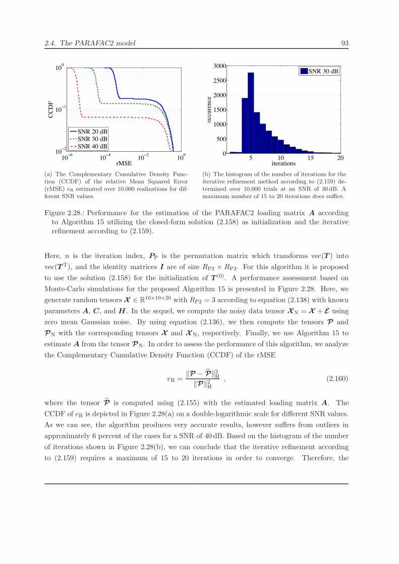
2.4. The PARAFAC2 model 93
10−6 10−4 10−2 10010−2
10−1
100
rMSE
CCD
F
SNR 20 dBSNR 30 dBSNR 40 dB
(a) The Complementary Cumulative Density Func-tion (CCDF) of the relative Mean Squared Error(rMSE) eR estimated over 10.000 realizations for dif-ferent SNR values.
5 10 15 200
500
1000
1500
2000
2500
3000
iterations
occu
renc
e
SNR 30 dB
(b) The histogram of the number of iterations for theiterative refinement method according to (2.159) de-termined over 10.000 trials at an SNR of 30 dB. Amaximum number of 15 to 20 iterations does suffice.
Figure 2.28.: Performance for the estimation of the PARAFAC2 loading matrix A accordingto Algorithm 15 utilizing the closed-form solution (2.158) as initialization and the iterativerefinement according to (2.159).
Here, n is the iteration index, PP is the permutation matrix which transforms vec(T ) into
vec(TT), and the identity matrices I are of size RP2 × RP2. For this algorithm it is proposed
to use the solution (2.158) for the initialization of T (0). A performance assessment based on
Monte-Carlo simulations for the proposed Algorithm 15 is presented in Figure 2.28. Here, we
generate random tensors X ∈ R10×10×20 with RP2 = 3 according to equation (2.138) with known
parameters A, C, and H. In the sequel, we compute the noisy data tensor XN = X + E using
zero mean Gaussian noise. By using equation (2.136), we then compute the tensors P and
PN with the corresponding tensors X and XN, respectively. Finally, we use Algorithm 15 to
estimate A from the tensor PN. In order to assess the performance of this algorithm, we analyze
the Complementary Cumulative Density Function (CCDF) of the rMSE
eR =∥P − P∥2H∥P∥2H
, (2.160)
where the tensor P is computed using (2.155) with the estimated loading matrix A. The
CCDF of eR is depicted in Figure 2.28(a) on a double-logarithmic scale for different SNR values.
As we can see, the algorithm produces very accurate results, however suffers from outliers in
approximately 6 percent of the cases for a SNR of 40 dB. Based on the histogram of the number
of iterations shown in Figure 2.28(b), we can conclude that the iterative refinement according
to (2.159) requires a maximum of 15 to 20 iterations in order to converge. Therefore, the

94 2. Multi-dimensional signal decompositions
complete procedure can still be considered closed-form.
2.4.4. A model order selection technique for the PARAFAC2 model
In this section, we present a new Model Order Selection (MOS) technique for the PARAFAC2
model. Thereby, it has to be noted that this problem has not been addressed in the literature
up to date. Before we derive the actual MOS technique, we define the PARAFAC2 model order
RP2 as the number of PARAFAC2 components under noisy observations. Therefore, we assume
that RP2 is the number of PARAFAC2 components of a third order signal tensor X such that
its PARAFAC2 decomposition according to equation (2.131) is exactly fulfilled. Then RP2 is
the model order of the tensor XN
XN = X + E , (2.161)
which represents an observation of X under additive noise E . For the PARAFAC2 model order
estimation we assume the following PARAFAC2 approximation of XN
(XN)i3=k = A · diag(dk) · F T · Vk , (2.162)
where the number of components is the predefined candidate model order PP2. Similar to the
basic idea of the direct fitting algorithm [126] (cf. Section 2.4.3.1) we can now transform the
PARAFAC2 approximation of XN to the new tensor
(XN
)i3=k
= (XN)i3=k · VTk = A · diag(dk) · F T , (2.163)
since the matrices Vk are unitary because of the Harshman constraint (2.135), i.e., Vk ·V Tk = I.
Here, it is possible to determine the PARAFAC2 model order of the tensor XN by performing
a CORe CONsistancy DIAgnostics (CORCONDIA) [42] on the transformed tensor XN defined
by equation (2.163). This is achieved (cf. Section 2.3.4) by analyzing the one-mode unfolding
of XN ∈ CI1×PP2×I3[XN
](1)
= A ·CPP2 · (C ⊗ F )T , (2.164)
with C = [d1, . . . ,dI3 ]T. In order to compute the core consistency, we have to estimate the
matrix CPP2 from equation (2.164) in least squares sense by
vec (CPP2) = (C ⊗ F ⊗A) · vec(X)
. (2.165)

2.4. The PARAFAC2 model 95
1 2 3 4 5 6 7 8
0
20
40
60
80
100
10 dB20 dB30 dB
e CC(P
P2)
candidate model order PP2
Figure 2.29.: The PARAFAC2 core consistency profile eCC(PP2) for a tensor of size 32×64×21.The model order was chosen to 3. A clear and abrupt descent in the consistency profile isrecognized at a candidate model order of P = 3 for all SNR values.
Using the matrix CPP2 we can now compute the PARAFAC2 core consistency of the tensor XN
in analogy to Section 2.3.4 as
eCC(PP2) = 100 ·
⎛
⎜⎝1−
∥∥∥CPP2 − [IN,PP2 ](1)
∥∥∥2
F
∥CPP2∥2F
⎞
⎟⎠ . (2.166)
Thereby, the PARAFAC2 CORCONDIA is based on the fact that without noise and the condi-
tion that model order RP2 is equal to the candidate model order PP2 it is CPP2 = [IN,PP2 ](1).
In this case, the core consistency is eCC = 100. For practical scenarios we have to compute
the PARAFAC2 core consistency (2.166) for a predefined range of candidate model orders, and
analyze the profile eCC(PP2) subjectively. Thereby, the core consistency remains close to 100 as
long as the candidate model order PP2 remains smaller or equal to the model order RP2 of the
tensor XN. As soon as the candidate model order exceeds the model order RP2 a steep descend
in the profile eCC(PP2) is observed.
In Figure 2.29 typical core consistency profiles for different SNRs are depicted. Thereby, the
tensor XN is of model order 3 and the size is 32 × 64 × 21, which is typical for the EEG
applications in Section 4.3. As expected, a steep descent in the core consistency profile is
observed from the candidate model orders 3 to 4 for all SNR values. In comparison to the
CORCONDIA for the PARAFAC model (cf. Section 2.3.4), it has to be noted that the novel
PARAFAC2 CORCONDIA requires an approximately 10 dB higher SNR in order to show an
unique steep descent at the model order RP2. In Algorithm 11 we summarize all necessary
computational steps in order to determine the core consistency profile (2.166), which is the basis

96 2. Multi-dimensional signal decompositions
Algorithm 11 The algorithm for the computation of the PARAFAC2 core consistency pro-file (2.166), which is the basis for the novel subjective PARAFAC2 CORCONDIA for ModelOrder Selection.Require: Third order Tensor XN ∈ CI1×I2×I3 and the maximum candidate model order Pmax
• for PP2 = 1, 2, . . . , Pmax
– compute the PARAFAC2 estimation using the direct fitting Algorithm 10 of XN
using the number of components PP2 obtaining the parameters A, C, F , Vk
– for k = 1, 2, . . . , I3∗(XN
)i3=k
= (XN)i3=k · VTk
end
– CPP2 = unvec((C ⊗ F ⊗A) · vec
(XN
))∈ C
PP2×P 2P2
– eCC(PP2) = 100 ·
⎛
⎜⎝1−
∥∥∥CPP2 − [IN,PP2 ](1)
∥∥∥2
F
∥CPP2∥2F
⎞
⎟⎠
end
• return eCC(PP2)
for the novel subjective PARAFAC2 CORCONDIA method.
2.4.5. Comparison between the PARAFAC and the PARAFAC2 model
In Section 2.4.1, we derived the PARAFAC2 model for a third order tensor X ∈ CI1×I2×I3
as a generalization of the PARAFAC model discussed in Section 2.3. In order to highlight
the differences between these two decomposition methods, we compare their structure as well
as their main properties in Table 2.8. First, both decomposition methods can be compared
directly based on their slice-wise representations (2.131) and (2.47). From this comparison we
can conclude that the PARAFAC2 model is a generalization of the PARAFAC model, where the
two-mode loadings Bk are allowed to vary over the third dimension indexed by k = 1, . . . , I3. In
PARAFAC2 an arbitrary loading matrix can vary over an arbitrary second dimension. However,
for the sake of simplicity and without loss of generality we always assume that Bk changes over
the third dimension. With the variable two-mode loading matrices Bk, the PARAFAC2 model
is much more general than PARAFAC and the available degrees of freedom are significantly
increased. However, with this increase in degrees of freedom there is also the necessity of the
Harshman constraint (2.135) in order to ensure the uniqueness of the PARAFAC2 model.
A second way of comparing PARAFAC and PARAFAC2 directly is enabled by the new component-
wise formulation of PARAFAC2 (2.132), which can be compared to the component-wise PARAFAC

2.4. The PARAFAC2 model 97
Property PARAFAC PARAFAC2
frontal slicestructure
!"#$%&'()*+,-./0123456789:;<=>?@ABCDEFGHIJKLMNOPQRSTUVWXYZ[\]^_`abcdefghijklmnopqrstuvwxyz{|}~
=
X A diag(dk) BT
!"#$%&'()*+,-./0123456789:;<=>?@ABCDEFGHIJKLMNOPQRSTUVWXYZ[\]^_`abcdefghijklmnopqrstuvwxyz{|}~
=
X A diag(dk) BTk
slice formulation (X )i3=k = A · diag (dk) ·BT (X )i3=k = A · diag (dk) ·BTk
componentstructure
!"#$%&'()*+,-./0123456789:;<=>?@ABCDEFGHIJKLMNOPQRSTUVWXYZ[\]^_`abcdefghijklmnopqrstuvwxyz{|}~
= =
Yr
ar
br
cr
ar bTr · cr
!"#$%&'()*+,-./0123456789:;<=>?@ABCDEFGHIJKLMNOPQRSTUVWXYZ[\]^_`abcdefghijklmnopqrstuvwxyz{|}~
=
Zr ar Gr · diag(cr)
componentformulation
X =R∑
r=1
ar ◦ br ◦ cr︸ ︷︷ ︸Yr
X =RP2∑
r=1
ar ◦ (Gr · diag(cr))︸ ︷︷ ︸Zr
component rank rank (Yr) = 1 1 ≤ rank(Zr) ≤ min(I2, I3)
n-mode loadingsnot unitary not unitary
A ∈ CI1×R, B ∈ CI2×R A ∈ CI1×RP2 , Bk ∈ CI2×RP2
C ∈ CI3×R C ∈ CI3×RP2 , k = 1, . . . , I3uniquenessconstraint
rank (Yr) = 1 BTk ·Bk = H
model orderselection
CORCONDIA or others PARAFAC2 CORCONDIA
component weightscomponent amplitudes component amplitudesγr with r = 1, . . . , R γr with r = 1, . . . , RP2
computationalcomplexity
high higher than PARAFACsemi-algebraic or iterative solution withiterative solution direct fitting Algorithm 10
Table 2.8.: Comparison of the structure and the main properties of the PARAFAC and thePARAFAC2 decomposition.
formulation (2.43). Thereby, we can conclude that the PARAFAC component tensors Yr are of
tensor rank-one, i.e., they are given by the outer product of a vector ar and a rank-one matrix
bTr · cr. In contrast to this, the PARAFAC2 component tensors Zr are created by the outer
product of a vector ar and a matrix Gr ·diag(cr), which can be of full rank. Since the maximum
rank of the matrix Gr is given by min(I2, I3), the tensor rank of the PARAFAC2 component
tensors Zr is in the range 1 ≤ rank(Zr) ≤ min(I2, I3).
For the application of both PARAFAC and PARAFAC2 in practical scenarios, the determination

98 2. Multi-dimensional signal decompositions
of the number of components (model order) is crucial. Unfortunately, this can be a challenging
problem for both decompositions. In the case of PARAFAC a lot of research has been dedicated
to this problem [60], and methods such as CORCONDIA, N -D AIC, N -D MDL and many
more are available (cf. Section 2.3.4). For the MOS in the case of PARAFAC2 we propose the
PARAFAC2 CORCONDIA scheme developed in Section 2.4.4. Together with the problem of
MOS, there is the problem of how to evaluate the influence of the different components. In
order to do this we propose to use the component amplitudes for PARAFAC according to (2.60)
and for PARAFAC2 according to (2.146). Furthermore, the inherent ambiguities are reduced in
both models when using these new normalization methods.
In terms of the computational complexity it has to be noted that PARAFAC2 usually requires
a much higher effort than PARAFAC. This is because the only practically applicable algorithm
available for PARAFAC2 is the direct fitting approach according to Algorithm 10 [126]. This
algorithm is based on ALS iterations which involve a complete PARAFAC decomposition within
every iteration (although the maximum number of iterations to solve this implicit PARAFAC
problem can be restricted to be very low, cf. Section 2.4.3.1). In contrast to this, there are
much more algorithms available in order to efficiently solve PARAFAC both of iterative and
semi-algebraic nature, which are also capable to exploit certain symmetries in the data tensors
(cf. Section 2.3.3).
2.4.6. Applications of the PARAFAC2 model
In comparison to the PARAFAC decomposition or the HOSVD, the PARAFAC2 model has been
rarely used in the literature up to date. The concept for the PARAFAC2 decomposition was orig-
inally introduced in 1972 by Harshman [94]. However, an efficient algorithm for the computation
of PARAFAC2 was not available at that time. Therefore, the first application of PARAFAC2
was presented by R. Bro et al. in 1999 [40] in the field of chemometrics, when also the direct
fitting algorithm [126] was available. Thereby, the PARAFAC2 model is used to analyze chro-
matographic data including retention time shifts. Later, in 2001 PARAFAC2 was used for the
fault detection in a chemical semiconductor etch process [212]. Furthermore, PARAFAC2 was
applied to the clustering of multi-lingual documents in the field of cross-language information
retrieval [49].
The PARAFAC2 model was first applied in the field of biomedical signal processing in [17].
Thereby, PARAFAC2 is used to analyze EEG as well as ECG data along the space (channels)
and time dimension in multiple segments. Furthermore, in [138] a PARAFAC2 based tensor
factorization method for the separation of speech signals is developed. PARAFAC2 is also used

2.5. Other tensor decompositions 99
for the detection and sorting of neural spikes in [6]. In the contributions [11–14], PARAFAC2
was introduced to the analysis of space-time-frequency atoms in measured EEG data and thereby
achieved significantly better results than the PARAFAC model. In the Chapters 3 and 4 this
PARAFAC2 based EEG decomposition strategy is discussed in detail.
2.5. Other tensor decompositions
At this point, we described three different tensor decomposition models, namely the HOSVD,
the PARAFAC and the PARAFAC2 model in the Sections 2.2, 2.3 and 2.4, respectively. Apart
from these three most widely applied tensor decompositions, many other multi-dimensional
decomposition models have been proposed in literature [128]. However, since the applicability of
these models to the field of neural signal processing has not yet been proven, we discuss them only
very briefly in the following two sections. Thereby, we present the class of Tucker decompositions,
which also includes the HOSVD, in Section 2.5.1. In Section 2.5.2, we discuss a short list
of other tensor decompositions which are distantly related to the PARAFAC decomposition.
Finally, in Section 2.5.3 we mention the class of Non-negative Tensor Factorizations (NTF). For
a comprehensive overview on the different tensor decompositions available in literature we refer
the reader to [21,128].
2.5.1. The Tucker decomposition model
The idea for the Tucker decomposition was originally introduced in 1963 by L. R. Tucker. Three
years later, in 1966 a more comprehensive and refined description of the model was presented
by Tucker in [196]. Thereby, it was the general goal of Tucker to generalize matrix factorization
methods to three-way arrays. The general class of Tucker decompositions for three-way arrays
X shows the following structure
X = G ×1 A×2 B ×3 C . (2.167)
Here, the loading matrices A, B and C are usually assumed to be orthogonal. It has to be
noted that even with an orthogonality constraint on the loading matrices, the decomposition
model (2.167) is not uniquely defined. Therefore, L. De Lathauwer et al. introduced the HOSVD,
which represents an unique Tucker decomposition by choosing the n-mode loading matrices
to be the matrices of the left singular vectors of the n-mode unfoldings, and by defining an
unique all-orthogonal core-tensor G. Also other researchers have used the Tucker decomposition

100 2. Multi-dimensional signal decompositions
model (2.167) under a confusing amount of different names. Some of the names which have been
used in literature and correspond to a Tucker decomposition are according to [128]
• Three-mode factor analysis;
• Tucker3 decomposition;
• N -mode Principal Component Analysis (PCA);
• Higher Order Singular Value Decomposition (HOSVD);
• N -mode SVD.
In the scope of this thesis the Tucker model (HOSVD) is used to implement the Tucker com-
pression (truncated HOSVD), which is used for the computation of the Closed-Form PARAFAC
(CFP) algorithm in Section 2.3.3.2 and for the efficient estimation of the PARAFAC2 one-mode
loading matrix A in Section 2.4.3.2. Furthermore, the Tucker compression is used for the com-
putation of the Khatri-Rao Factorization (KRF) as derived in Appendix B.7. Therefore, it is
required in many PARAFAC related methods, such as the CFP and the ProKRaft algorithm
in Section 2.3.3.3. The Tucker compression often leads to estimation problems of reduced size
hence enabling more effective estimation procedures.
2.5.2. Tensor decompositions related to PARAFAC or PARAFAC2
According to [128] there are at least five different tensor decompositions that are either related
to PARAFAC or to PARAFAC2. These tensor decompositions are listed in Table 2.9 together
with the corresponding references providing more informations about these models. The first
PARAFAC related tensor decomposition to note here is the INdividual Differences in SCALing
(INDSCAL) model, which represents a three-way PARAFAC where the one-mode and the two-
mode loading matrices are equal, such that INDSCAL reads as
X = I3,R ×1 A×2 A×3 C . (2.168)
Another tensor decomposition, which is directly related to PARAFAC, is the CANDECOMP
with LINear Constraints (CANDELINC) model. It represents a PARAFAC model, where linear
constraints can be imposed on all loading matrices in the form of unitary constraint matrices
(please note that CANDECOMP is another term for PARAFAC). In recent literature, re-
searchers also introduced tensor decomposition models such as PARAllel profiles with LINear

2.5. Other tensor decompositions 101
Decomposition Reference Annotation
Higher Order Singular Value De-composition (HOSVD)
cf. Section 2.2 n-rank based generalization of thematrix SVD
PARAllel FACtor (PARAFAC)Analysis
cf. Section 2.3 tensor rank based generalization ofthe matrix SVD
INdividual Differences in SCAL-ing (INDSCAL)
cf. [47] 3-way PARAFAC where one-modeloadings equal two-mode loadings
CANDECOMP with LINearConstraints (CANDELINC)
cf. [48] PARAFAC with linear constraintson the loading matrices
PARallel FACtor2 (PARAFAC2)Analysis
cf. Section 2.4 generalization of PARAFAC
DEcomposition into DIrectionalCOMponents (DEDICOM)
cf. [95] generalization of PARAFAC2
PARAFAC and TUCKer2(PARATUCK2)
cf. [97] generalization of DEDICOM
PARAllel profiles with LINearDependencies (PARALIND)
cf. [21, 41] Decomposition into a number ofcomponents with low n-rank Tuckerstructure
Table 2.9.: Overview of tensor decompositions found in literature.
Dependencies (PARALIND), which try to relax the rank-one constraint on the PARAFAC com-
ponents. This is achieved by introducing dependency matrices which model the interactions
between different components. Thereby, every component can have a different rank.
The DEcomposition into DIrectional COMponents (DEDICOM) model represents a generaliza-
tion of the PARAFAC2 model based on its cross-product representation (2.136). The DEDICOM
model is given by
P = A · diag(dk) ·Φ · diag(dk) ·AT , (2.169)
where in contrast to PARAFAC2, the matrixΦ is not restricted to be symmetric positive definite.
An even more general model is given by PARAFAC and TUCKer2 (PARATUCK2), which in
comparison to (2.169) reads as
P = A · diag(dk) ·Φ · diag(ek) ·BT . (2.170)
102 2. Multi-dimensional signal decompositions
2.5.3. Non-negative tensor decompositions
In many applications the loading matrices of the PARAFAC decomposition correspond to phys-
ical dimensions which are not allowed to assume negative values. For these applications, Non-
negative Tensor Factorization (NTF) methods have been developed which are usually based on
a PARAFAC model with an additional non-negativity constraint on the loading matrices. The
NTF models are also used for the processing of neurological data, like EEG or MEG. For a
comprehensive overview on NTF and its applications, the reader is referred to [52].
2.6. Summary
In this Chapter, we investigated the three tensor decompositions which are applied to the com-
ponent analysis of neurological multi-channel data in this thesis. Those tensor decompositions
are namely, the Higher Order Singular Value Decomposition (HOSVD), the PARAllel FAC-
tor (PARAFAC) decomposition and the PARAllel FACtor2 (PARAFAC2) decomposition. We
introduced both the HOSVD and the PARAFAC decomposition as multi-dimensional gener-
alizations of the matrix Singular Value Decomposition (SVD) in Section 2.1. The HOSVD
analyzes a data tensor X as a collection of n-mode vectors which are straight forward general-
izations of the column and row vectors of a matrix. In the same way as the matrix SVD, the
HOSVD provides an unitary basis of the n-mode vector spaces in its loading matrices. Further-
more, the HOSVD reveals the n-ranks, which represent the dimensions of the n-mode vector
spaces. This convincing concept of generalizing the matrix SVD to the multi-dimensional case
is discussed in Section 2.2, where also all the properties relevant to this thesis are analyzed
in detail. Additionally, we provided the algorithms for the computation of the HOSVD itself
(cf. Algorithm 1) as well as for its important applications including the truncated HOSVD (cf.
Algorithm 2) and the Higher Order Orthogonal Iterations (HOOI) method (cf. Algorithm 3). A
short survey of possible applications of the HOSVD was presented in Section 2.2.4. Throughout
this thesis, especially the truncated HOSVD is used for the computation of the Closed-Form
PARAFAC (CFP) algorithm in Section 2.3.3.2. This algorithm is applied in Chapter 4 as well as
for the estimation procedure for the PARAFAC2 one-mode loading matrix A in Section 2.4.3.2.
The HOOI represents an alternative to the truncated HOSVD, which is optimal in least squares
sense. However, it is computationally much more complex. Furthermore, the HOOI algorithm
can be used to determine the best rank-one approximation of a tensor, which is relevant for the
joint least squares Khatri-Rao Factorization (KRF) (cf. Appendix B.7).

2.6. Summary 103
In Section 2.3, we presented detailed investigations about the PARAFAC model and all the
properties relevant to this thesis. In this context, we introduced the PARAFAC component am-
plitudes in Section 2.3.2.4, which enable a normalized representation of PARAFAC. With this
normalization the scaling and permutation ambiguity in the PARAFAC components is reduced
to a sign ambiguity. Furthermore, this normalization concept allows to evaluate the influence
of the different PARAFAC components, and enables us to combine different estimates of the
PARAFAC loading matrices in order to increase the performance of PARAFAC algorithms. Es-
pecially this last possibility is exploited for example in the CFP algorithm in Section 2.3.3.2,
which is used for the decomposition of EEG signals in Chapter 4. In the presentation of the
PARAFAC properties in Section 2.3.2 we also included the class of dual-symmetric tensors (cf.
Section 2.3.2.5). In the subsequent sections about PARAFAC algorithms we derived the Pro-
crustes estimation and Khatri-Rao factorization (ProKRaft) algorithm (cf. Section 2.3.3.3),
which is able to exploit the structure of dual-symmetric tensors. Our results show that the
ProKRaft algorithm outperforms current state-of-the-art approaches. Furthermore, we exploited
the connection between PARAFAC and the computation of the Independent Component Anal-
ysis (ICA) in order to provide a ProKRaft based ICA algorithm. The possibility to compute
the ICA via ProKRaft shows the great potential of this algorithm to be applied in many dif-
ferent Blind Source Separation (BSS) problems. Finally, we compared the PARAFAC model
to the HOSVD in Section 2.3.5 before presenting a survey of PARAFAC applications found in
literature in Section 2.3.6. In this thesis, we use the PARAFAC model as the state-of-the-art
method for the extraction of the components of neural processing in Chapter 4. Thereby, we
generally make use of the CFP Algorithm 6. The ProKRaft based ICA algorithm can be used
for the artifact removal in the time-domain of EEG data. Furthermore, the iterative PARAFAC
approaches presented in Section 2.3.3.1 are used for the computation of PARAFAC2.
The PARAFAC2 model was investigated in detail in Section 2.4. Thereby, we defined the
PARAFAC2 model in Section 2.4.1 as a three-way tensor decomposition, which can be seen as
a generalization of the PARAFAC model. The PARAFAC2 model is more flexible than the
PARAFAC model since it supports the variation of one of the loading matrices over a second
dimension. Please notice that in this thesis, we only consider the special case of the PARAFAC2
decomposition for tensors. The PARAFAC2 model is described with a special focus on its
different mathematical representations. Thereby, we also introduced the component-wise repre-
sentation (2.132) as well as a new compact cross-product representation (2.137) of PARAFAC2,
which is derived in Section 2.4.3.2. The component-wise representation of PARAFAC2 enabled
us to introduce a normalization method for PARAFAC2 in Section 2.4.2.2, which is very similar
to the normalization of PARAFAC in Section 2.3.2.4. Again, by applying this normalization
the scaling and permutation ambiguity in PARAFAC2 is reduced to a sign ambiguity. Fur-

104 2. Multi-dimensional signal decompositions
ther, it allows to evaluate the influence of the different PARAFAC2 components. Based on
the cross-product representation (2.137) of PARAFAC2 we developed new and efficient algo-
rithms for the separate estimation of the one-mode and three-mode loading matrices in Sec-
tion 2.4.3.2. Furthermore, we presented a Model Order Selection (MOS) technique for the
PARAFAC2 model in Section 2.4.4 by transforming the model such that CORe CONsistancy
DIAgnostics (CORCONDIA) (cf. Section 2.3.4) can be applied. Finally, we presented a com-
parison between PARAFAC and PARAFAC2 in Section 2.4.5 before presenting a brief survey
of PARAFAC2 applications in Section 2.4.6. Throughout this thesis, the PARAFAC2 model is
used as the basic tool for a EEG decomposition strategy introduced in Chapter 3. This strat-
egy is based on the analysis of space-time-frequency atoms and exploits the greater flexibility
of the PARAFAC2 model over PARAFAC in order to incorporate additional physiological ef-
fects. For the computation of PARAFAC2 we generally use the direct fitting approach presented
in Section 2.4.3.1. The PARAFAC2 based EEG decomposition strategy represents one of the
main contributions of this thesis and its advantages over existing EEG space-time-frequency
decompositions are investigated in Chapter 4.

105
3. EEG signal decomposition strategies
The signals measured by the ElectroEncephaloGram (EEG) are generated from the superposi-
tion of the activity of multiple neural sources as well as from biological artifacts and technical
distortions. Therefore, Blind Source Separation (BSS) methods are required in order to separate
the desired components of neural activity and to suppress the artifacts and distortions. In this
chapter, we investigate and compare the theoretical nature of different EEG signal decomposi-
tion strategies, which aim to separate the scalp projections of the contributing neural sources.
The extracted scalp projections enable a separate topographic analysis of the components of
neural activity, which represents one of the key scientific and diagnostic tools in neurology [185].
Throughout this thesis, we focus especially on multi-dimensional EEG decomposition strategies
which include tensor decompositions such as PARAFAC or PARAFAC2. Thereby, we exploit
the theoretical advantages of tensor decompositions over 2D decomposition methods such as the
Singular Value Decomposition (SVD) or the Independent Component Analysis (ICA). Please
note that the term EEG decomposition strategy, used throughout this thesis, also includes other
processing steps such as the Time-Frequency Analysis (TFA).
The main contribution of this chapter is the multi-dimensional EEG decomposition strategy
based on the PARAFAC2 model introduced in Section 3.3.3. This decomposition strategy is
able extract the temporal evolution of virtually moving neural sources. Furthermore, we inves-
tigate the application of Wigner-based TFA methods for multi-dimensional EEG decomposition
strategies in Section 3.4.
In the following Section 3.1, we discuss the physiological origins of the EEG before presenting
the current state of the art on EEG decomposition strategies in Section 3.2. In Section 3.3, we
describe the EEG decomposition strategies considered throughout this thesis. Thereby, we focus
especially on the theoretical assumptions which these methods impose on the neural sources.
Possible methods for the TFA, which are required for the multi-dimensional EEG decomposi-
tion strategies, are discussed and evaluated in Section 3.4. Finally, we compare the inherent
assumptions of all considered EEG decomposition strategies in Section 3.5 before presenting the
summary of this chapter in Section 3.6.

106 3. EEG signal decomposition strategies
3.1. The physiological foundation of the EEG
The origins of the ElectroEncephaloGram (EEG) date back to the year 1924, when the german
neurologist Hans Berger carried out the first EEG measurements. After five years of research
Berger pointed out that the measured differences in the electric potential at the scalp, measured
by EEG, must have their source in the human brain and therefore excluded other possible sources
such as muscle activity or the activity of the heart [213].
Indeed the EEG is mainly generated from sources in the cerebral cortex, which represents the top
layer of the brain tissue with a thickness of approximately 2.5mm (see Figure 3.1a). The main
parts of the brain tissue consists of two types of cells, namely the Glia cells and the neurons.
The function of the Glia cells includes physical support of neuron structures, the generation of
myelin as well as the maintenance of homeostasis in the brain. Over the last decades, these
Glia cells where considered to be passive in the sense that they are not able to produce action
potentials or synaptic potentials. However, in recent investigations it has been observed that
Glia cells are also able to trigger synaptic potentials [153] and therefore influence the activity of
neurons. Apart from these minor interactions of the Glia cells and neurons, the influence of Glia
cells on the EEG is considered to be negligible [27]. The main contribution to the differences in
the electrical potential, which is measured by the EEG at the surface of the scalp, is caused by
the activity of neurons.
If a neuron is activated, it produces a short action potential at the membrane of the cell [30].
This action potential is caused by a depolarization between the extra-cellular space and the
intra-cellular space. In case of no activation, the intra-cellular space usually shows a potential
of -70mV in comparison to the extra-cellular space [91]. After the depolarization, which causes
the action potential of the activated neuron, a fast repolarization takes place. The whole process
of depolarization and repolarization has a duration in the range of 1ms to a few ms. Therefore,
action potentials are causing signals in a high frequency range (around 500Hz), which are usually
not supported by standard EEG systems. Furthermore, the high-resistance EEG electrodes at
the surface of the scalp are to far away from the cell membranes in order to be influenced
by action potentials. However, action potentials are transmitted along the axon to the axon
terminal, which is part of the synapse. There, they can trigger a synaptic potential signaling
other neurons.
Synaptic potentials are caused by chemical transmitter substances such as glutamate (excitatory)
or GABA (inhibitory), which induce differences in the cell membrane potential by opening or
closing certain ion channels. The subsequent ion currents caused by these neurotransmitters
are slow and strong enough to contribute to the differences in the electrical scalp potentials

3.1.Thephysiological
foundation
oftheEEG
107
I
II
III
IV
V
VI
dendritic tree
apicaldendrites
synapse
soma
axon basal
dendrites
cerebralcortex
scull
scalp
cerebrospinalfluid
frontallobe
occipitallobe
temporal lobe
parietallobe
cutting plane(see below)
gyrus
sulcuscentralis
sulcuslateralis
sulc
us
macro columns
c)b)a)
tangentialsource
radial source
right hemisphere
cerebral cortex
axonterminal
Figure 3.1.: The structure of the cerebral cortex, which represents the top layer of the brain with a thickness of approximately2.5mm. Figure a shows the brain lobes as well as the cerebrospinal fluid, the scull and the scalp of the head. Figure bdepicts the folded structure of the cerebral cortex including gyri and sulci. Figure c shows the 6 layers of the cerebral cortexincluding the parallel pyramidal neurons mainly generating the EEG.

108 3. EEG signal decomposition strategies
measured by the EEG electrodes. The synaptic potentials appear, e.g., at the synapses along
the dendritic trees of the pyramidal neurons in the cerebral cortex (see Figure 3.1c). If a neuron
is activated there by an excitatory neurotransmitter, such as glutamate, a depolarization at the
dendrite is observed. This leads to a negative potential in the extra-cellular space at the surface
of the neuron (dendrite).
The difference in the electric scalp potential caused by a synaptic potential of a single neuron is
far too weak to be recognized by an EEG electrode placed at the surface of the scalp. In order to
generate a difference in the scalp potential large enough to be recognized by EEG electrodes at
least many 10.000 to 100.000 neurons have to be activated simultaneously such that the extra-
cellular field potentials add up. This is only possible if these neurons are arranged in parallel,
such as the pyramidal neurons located in the cerebral cortex. This is also the reason why this
area of the human brain mainly contributes to the EEG.
The cerebral cortex is divided into 6 layers I to VI as depicted in Figure 3.1c. Thereby, layer I
contains the extensions of the apical dendritic tree. The layers II to III contain small to medium
size pyramidal neurons, while layer IV contains afferent fibers originating from neurons in the
thalamus, as well as afferent fibers connecting other structures in the cerebral cortex. Layer V
is mainly created by the cell bodies of large pyramidal cells whose axons and basal dendrites
reach subcortical structures. Finally, layer VI contains a smaller number of large pyramidal
neurons as well as smaller neurons creating both inhibitory and excitatory connections to the
thalamus. One of the functions of the thalamus, which is located between the cerebral cortex
and the midbrain, includes the relay of sensory signals and motor signals to the cerebral cortex.
The parallel structure of the apical dendrites originating from the larger pyramidal neurons
significantly contribute to the EEG.
Aside from its layered structure, the cerebral cortex is strongly folded in order to increase the
surface of the brain (see Figure 3.1a and b). Thereby, a turning in the curvature of the cerebral
cortex is termed a gyros whereas a groove is a termed sulcus. The parts of the cerebral cortex
which contain pyramidal cells oriented towards or away from the scalp surface, also termed radial
sources, contribute most to the EEG. The areas containing radial sources are found at the top
side and the lower side of the gyri. In contrast to this, areas with tangentially oriented sources
are found at the left and the right side of the sulci (Figure 3.1b). For a noticeable change in the
EEG, usually larger areas of the cerebral cortex have to be activated. Thereby, it happens often
that areas containing tangential sources in opposite direction are activated simultaneously. In
these cases the differences in the scalp potential caused by these opposing tangential sources
tend to cancel each other. Therefore, the contribution of the tangential sources to the EEG is
significantly diminished.

3.1. The physiological foundation of the EEG 109
!"#$%&'()*+,-./0123456789:;<=>?@ABCDEFGHIJKLMNOPQRSTUVWXYZ[\]^_`abcdefghijklmnopqrstuvwxyz{|}~
-1
0
1
+
b) -1
0
1
a)
Figure 3.2.: The electrical field potentials generated by sources in the cerebral cortex with dif-ferent orientations. Figure a shows the field potential of a radial source, while Figure b isgenerated from a tangential source. The radial source in a is located under the point wherethe magnitude of the field potential reaches its maximum. In contrast to this, the tangen-tial source in b is located at the point where the magnitude of the gradient of the bipolarfield potential reaches its maximum. Measured EEG data are mainly generated from radialsources.
The fact that mainly radial sources contribute to the EEG also influences the topographic
analysis of EEG data. Under the assumptions that only one radially orientated part of the
cerebral cortex is active, and that there is a perfectly indifferent (electrically neutral) reference
available for the EEG measurements, the activated brain area is located under the EEG electrode
showing the highest voltage magnitude. A topographic example of a radial source reflecting the
negative charges in the extra-cellular space at the left hemisphere between the frontal and the
temporal lobe is depicted in Figure 3.2a. In contrast to this, a source orientated tangentially to
the surface of the head is characterized by a bipolar field potential where the source is located
between the positive and the negative part of the potential at the point of the highest gradient
magnitude (see Figure 3.2b). Although the EEG is mainly created from radial sources, tangential
sources can appear in the early stages of evoked potentials (i.e., EEG measurements triggered
to a strong stimulus).
It has to be noted that the localization of both tangential and radial sources in the EEG is not
very accurate. One reason for this is found in the space between the brain and the surface of
the scalp, which includes the cerebrospinal fluid, the skull and the scalp (Figure 3.1a). Together
with the extra-cellular space in the cerebral cortex these layers build a non-homogeneous and
non-isotropic volume conductor whose exact electrical properties strongly depend on individual

110 3. EEG signal decomposition strategies
features. Furthermore, the standard EEG electrode setups, such as the international 10-20
system or the 10-10 system [150] (cf. Section 4.1.3), show relatively large electrode spacings of
approximately 6 cm (10-20 system) to 3 cm (10-10 system) on an average head of an adult person.
Therefore, these electrode setups do not comply with the spatial sampling theorem. In practical
scenarios, also the measurement noise as well as the resistivity of the scull restricts the spatial
resolution which can be obtained. A significant amount of research has been dedicated to the
question of how many electrodes have to be used in order to achieve a maximum spatial resolution
which is not mainly restricted by noise. In [167] it is shown that even for optimal circumstances
a number of 256 measurements electrodes should not be exceeded. This corresponds to a spacing
of approximately 1.6 cm. However, in typical clinical situations with higher noise levels a number
of 64 electrodes, which corresponds to the 10-10 system, does suffice.
The difficult nature of EEG is also reflected in the properties of the measured EEG signals. All
EEG measurements are affected by noise which exhibits an unknown amplitude distribution.
Furthermore, the signals often suffer from a very low Signal-to-noise Ratio (SNR) and the
noise can also show spatial correlation. In some cases, e.g., in single trial measurements of
evoked potentials, the SNR can reach values below -20 dB. Additionally, EEG data are often
superimposed by artifacts originating from other sources of the human body. These artifacts can
originate from muscle activity (EMG) or even from the activity of the heart (ECG). Desired
signal shapes which are expected for example in the measurements of evoked potentials are
often superimposed by EEG signals originating from spontaneous neural activity (also termed
background EEG). Also a wide variety of technical distortions can influence the EEG, such
as 50Hz line noise, motion artifacts and drifts caused by the changing impedance of the EEG
electrodes. It also has to be noticed that the signal characteristics of both the EEG including
the artifacts as well as the distortions may change over time. Therefore, EEG data has to be
considered non-stationary.
Since the EEG measures only the differences in the electrical field potential, a reference is
required against which all EEG channels are recorded. Because of safety reasons this reference
has to be obtained from the test person itself and is therefore not electrically neutral. In bipolar
measurements, which are not considered in this thesis, every EEG electrode exhibits its own
nearby placed reference electrode. In referential measurements all EEG electrodes are recorded
against one common reference. Standard references for these types of measurements are: the
central zero (Cz) electrode (cf. Section 4.1.3), the average earlobe reference ((A1 + A2)/2), or
the Common Average Reference. In comparison to the Cz or the average earlobe reference, the
CAR has the disadvantage of distributing artifacts over all EEG channels and it possibly creates
artificial potentials. Finally, it has to be mentioned that the choice of an adequate reference has

3.2. State of the art for EEG signal decomposition strategies 111
great influence on the interpretation and on the topographic analysis of EEG data [76].
3.2. State of the art for EEG signal decomposition strategies
Extracting the components of neural activity from event-related EEG data has been a long
standing problem in neurology. In 1978 E. Donchin and E. F. Hartley [73] pushed the analysis
of Event Related Potentials (ERP) beyond the simple extraction of peak amplitudes and latency
measures by introducing the Principal Component Analysis (PCA) to this problem. In these
applications of the PCA, different time points of the EEG data serve as variables, while different
subjects as well as different measurement electrodes are used as observations. In a topographical
analysis approach, W. Skrandies and D. Lehmann have used the PCA in order to decompose
the electrical brain fields of the underlying components [187]. Based on this work, the PCA has
also been used for artifact removal and to extract significant activities in EEG data [131, 188].
Furthermore, the PCA has been applied for the topographic analysis of Visual Evoked Potentials
(VEP) [185, 186]. A basic limitation of two-dimensional (2D) analysis techniques is that the
components are defined only over two dimensions (e.g., space and time) and therefore are not
determined uniquely. In PCA this problem is solved by imposing an orthogonality constraint
on the signatures of the corresponding components. However, even with the orthogonality
(uncorrelated sources) requirement a remaining ambiguity in PCA allows arbitrary rotations of
axes (e.g., Varimax rotations).
In order to overcome the rotational indeterminacy of the PCA, more recently the Independent
Component Analysis (ICA) [55] has been used to uniquely identify the space-time components
of neural activity [51,109]. In this context, the ICA is also used for the artifact rejection in EEG
data. Compared to PCA the ICA avoids the rotational non-uniqueness by imposing a more
restrictive constraint than orthogonality on its source signals, namely statistical independence.
In general, two-dimensional decomposition techniques (e.g., PCA and ICA) have to impose arti-
ficial constraints, like orthogonality or statistical independence, in order to extract unique source
signals. For the extraction of the components of neural activity in EEG data, these constraints
do not show any neuro-physiological correspondence. To overcome this problem J. Mocks [141]
suggested the topographic component model in 1988, based on biophysical considerations, for
the analysis of Event Related Potentials. In 1991 A. S. Field and D. Graupe [79] showed that
the topographic component model is a mathematical equivalent of the well-known PARAllel
FACtor (PARAFAC) analysis, which was derived independently by R. A. Harshman [93] and
J. D. Carroll et al. [47] in 1970. Furthermore, A. S. Field and D. Graupe [79] gave examples
112 3. EEG signal decomposition strategies
illustrating the utility of PARAFAC for the analysis of ERP and also discussed some practical
aspects (scaling and permutation, etc.). The PARAFAC decomposition (also called Canonical
Decomposition) decomposes a multi-dimensional (at least three dimensional) signal into a sum
of rank-one components. Thereby, the PARAFAC model shows some very important unique-
ness properties [36] which enable us to identify the rank-one components without imposing
any artificial constraints (cf. Section 2.3). Therefore, the PARAFAC analysis shows a supe-
rior performance for the extraction of neural components over two dimensional decompositions
like ICA [189] (cf. Chapter 4). Please note that applying the PARAFAC model to standard
space (electrodes)-time EEG measurements, requires an additional diversity (i.e., an additional
dimension like frequency, subjects, trials, etc.).
Based on the above mentioned initial contributions, other researchers have started to use the
PARAFAC model for the analysis of EEG data. In 2001 F. Estienne et al. [78] investigated the
influence of drugs on the EEG data of multiple subjects by performing a PARAFAC analysis
over a six-dimensional data array incorporating the dimensions frequency band, subject, space
(electrodes), drug dose, time, and measurement condition. In 2004 F. Miwakeichi et al. [140]
suggested one of the nowadays most popular multi-way analysis schemes, which decomposes EEG
data into space-time-frequency components. This is achieved by performing a time-frequency
analysis (e.g., short time Fourier-transform, Wavelet transform, etc.) on each EEG channel, and
a subsequent PARAFAC decomposition (cf. Section 3.3). Later in 2006 M. Mørup et al. [146]
further investigated this idea for the special case of Wavelet-transformed event-related EEG
data. In 2006 K. Nazarpour et al. [148] demonstrated the utility of the PARAFAC model in the
context of Brain Computer Interfaces (BCI) by developing a hybrid “parallel factor analysis-
support vector machine” method for left and right imagery movement classification. Recently, in
2007 the space-time-frequency analysis using PARAFAC was also applied to investigate epileptic
seizures by E. Acar et al. [18, 19]. Additionally, M. de Vos et al. [203, 206] showed that this
analysis concept is also able to detect epileptic seizure onset zones in a noninvasive fashion.
Thereby, the PARAFAC decomposition is used in order to separate the scalp projections of the
different neural sources. In the sequel, the spatial location of each source is identified by a dipole
fitting method [142,204].
For the computation of the PARAFAC model a significant amount of research was dedicated
to iterative methods to estimate the rank-one components from noisy data. In many situa-
tions these iterative algorithms require many iterations and are not guaranteed to converge to
the global optimum. In 2008 F. Roemer and M. Haardt [163, 164] developed a closed-form
semi-algebraic solution for the PARAFAC model, which outperforms the iterative approaches
especially in critical scenarios (cf. Section 2.3.3.2). Furthermore, in 2008 J. P. C. L. da Costa
3.2. State of the art for EEG signal decomposition strategies 113
et al. [67] developed a robust method for estimating the number of components (model order)
in the PARAFAC model. In 2009 M. Weis et al. [4,16] compared the performance of numerous
linear and quadratic time-frequency analysis schemes (e.g., the Reduced Interference Distribu-
tion (RID)) and used the new developed closed-form semi-algebraic PARAFAC algorithm [163]
for the space-time-frequency analysis of visual-evoked potentials.
Recently, also other multi-way decomposition models [128] have been used in the context of EEG
data processing. In 2005 M. Mørup [143] compared different multi-way decomposition models
for the space-time-frequency analysis of EEG data, e.g., HOSVD [135], PARAFAC, and more.
In these studies the PARAFAC model showed the best performance. Furthermore, M. Mørup
et al. [147] proposed to include an additional non-negativity constraint into the decomposition
process by utilizing non-negative matrix and multi-way factorizations. This idea is also inves-
tigated in detail in [52]. In 2006 E. Acar et al. [19] compared different linear and non-linear
decomposition schemes in order to localize the focus of epileptic seizures. In this contribution
a novel non-linear multi-way decomposition algorithm, namely the kernelized Tucker3 model
was developed, which can be seen as a higher-order generalization of the kernelized PCA [176].
The outcome of these investigations shows that both the linear Tucker3 model [196] and the
non-linear (kernelized) Tucker3 model perform best at localizing the epileptic focus. Both de-
compositions are based on the space-time-frequency content of the EEG data. Very recently, in
2009 B. M. Adabi et al. [17] proposed the use of the PARAFAC2 decomposition for the space-
time-trial analysis of both EEG and the ElectroCardioGram (ECG). The PARAFAC2 model
can be seen as a generalization of the PARAFAC model in the sense that the components are
not necessarily restricted to be rank-one (cf. Section 2.4). Following the ideas of shifted factor
analysis for chromatographic data in [96,126], the PARAFAC2 model was proposed in [11–14]
for the decomposition of EEG data into space-time-frequency atoms, which appear time shifted
over the different channels (cf. Section 3.3.3). These investigations show that the PARAFAC2
model outperforms the space-time-frequency PARAFAC analysis originally proposed in [140].
The superiority of this decomposition strategy was shown for the case of measured Visual Evoked
Potentials as well as for simulated EEG data [7].
Very recent investigations show that the consideration of other diversities than the frequency
dimension can lead to an improved decomposition process. In [32] a two-dimensional Fourier-
transform was applied to synthetic EEG in the spatial domain, in order to obtain a space-
time-wavevector representation of the data. A subsequent PARAFAC analysis using the closed-
form semi-algebraic PARAFAC algorithm [163] facilitates the application of a new dipole-fitting
method, which shows a superior performance over existing methods.
114 3. EEG signal decomposition strategies
3.3. Investigated EEG signal decomposition strategies
Very often EEG data are generated from multiple neural sources and they are contaminated by
artifacts, technical distortions and noise. Therefore, decomposition strategies are required in
order to extract the components of neural activity and to separate them from undesired signal
components. In the following, the term EEG decomposition strategy includes all processing steps
which are necessary to estimate the components of neural activity from the measured EEG data.
Therefore, a decomposition strategy not only includes the actual signal decomposition, such as
the ICA or PARAFAC, but also intermediate steps such as the Time-Frequency Analysis (TFA).
Throughout this thesis we mainly investigate EEG decomposition strategies which are based on
multi-dimensional signal decompositions, such as PARAFAC (Section 3.3.2) and PARAFAC2
(Section 3.3.3). However, we also consider one decomposition strategy based on the 2D signal
decomposition via the ICA in Section 3.3.1. This enables us to compare the 2D decomposition
strategies against the multi-dimensional decomposition strategies. From this comparison we
are able to prove that the increased amount of data and computational complexity involved in
multi-dimensional signal decomposition strategies gives rise to an increased performance in terms
of the quality of the extracted components as well as robustness against noise. The objective
comparison between all EEG decomposition strategies introduced in this section is treated in
Chapter 4 on the basis of synthetic and measured EEG data.
The multi-dimensional EEG decomposition strategies discussed in this thesis operate on the
three dimensions frequency, time and space (channels) and therefore lead to a representation
of the components of neural activity in terms of space-time-frequency atoms. The reason why
we mainly restrict ourselves to these diversities is twofold. First, standard EEG experiments
used in clinical applications, such as Visual Evoked Potentials (VEP), are very well investigated
in terms of their temporal evolution as well as their frequency content. Therefore, the multi-
dimensional decomposition strategies can be validated by evaluating the comparison between
the extracted space-time-frequency atoms and the known frequency-time properties of these
standard experiments. This possibility is of particular interest when analyzing measured EEG
data (cf. Section 4.3). Second, EEG signals are non-stationary hence their frequency content
has to be analyzed in its temporal evolution. Therefore, a TFA is necessarily included in the
multi-dimensional decomposition strategies.
It also has to be noted that all investigated EEG signal decomposition strategies in this thesis
assume a linear superposition of the neural sources and operate in the signal space, i.e., on
the measured EEG signals. Therefore, the techniques discussed here separate only the scalp
projections of the different neural sources. A vast amount of research has been dedicated to the

3.3. Investigated EEG signal decomposition strategies 115
separation of neural sources in the source space including the localization of those sources [23].
This is possible by incorporating possible solutions to the inverse problem (cf. Section 4.1.1)
in the decomposition process. Indeed it is also possible to use multi-dimensional decomposition
techniques such as PARAFAC for the source separation in the source space [31]. In this thesis
the inverse problem is not considered because its solution depends heavily on physiological pa-
rameters whose measurement is very complex and intra-individual [99–103]. Furthermore, the
solution to the inverse problem is in general not unique. However, the separation of sources can
also be achieved by applying a possible solution of the inverse problem (e.g, LOw Resolution
Electromagnetic TomogrAphy [154]), to the components estimated by the following decomposi-
tion strategies in order to obtain a combined separation and localization of the sources of neural
activity [142, 204]. Unfortunately, the investigation of these inverse techniques is beyond the
scope of this thesis.
In the following sections, we present the EEG decomposition strategies used throughout this
thesis and discuss their theoretical properties in detail. Thereby, we focus on the assumptions
which have to be imposed in order to extract the components of neural activity using the respec-
tive decomposition strategy. Please notice that we use an ambiguous mathematical notation for
the description of the following three EEG decomposition strategies. Thereby, we use the same
mathematical symbols for the corresponding quantities in the different methods (e.g., the matrix
containing the channel weights of the extracted components is always denoted by C ∈ RNC×R).
This simplifies the notation and helps to recognize common quantities extracted by the different
decomposition strategies.
3.3.1. Direct EEG decomposition using Independent Component Analysis
The first EEG signal decomposition strategy is based on the Independent Component Analysis
(ICA). This 2D decomposition strategy is very well investigated in literature [74] and serves as
a reference for the multi-dimensional methods covered in the following sections. In this strategy
the ICA is directly applied to the EEG measurement signals X of size NC × NT, where NC
and NT are the number of EEG channels and the number of time samples, respectively (cf.
Figure 3.3). Thereby, the ICA is based on the following linear mixing model
X = C ·BT . (3.1)
whereC ∈ RNC×R is the mixing matrix andB ∈ RNT×R is matrix of source signals. The variable
R denotes the number of components to be extracted. In order to be able to compare the ICA

116 3. EEG signal decomposition strategies
!"#$%&'()*+,-./0123456789:;<=>?@ABCDEFGHIJKLMNOPQRSTUVWXYZ[\]^_`abcdefghijklmnopqrstuvwxyz{|}~
chan
nel
time
chan
nel
time
chan
nel
time
Independent Component
Analysis
EEG Measurements
X
Y1
YR
Figure 3.3.: The EEG signal decomposition strategy based on the ICA. The ICA is directlyapplied to the EEG measurements X, which vary over the diversities channel and time. Theextracted independent components Y1, . . . ,YR are characterized by a channel signature anda time signature.
based decomposition strategy to the multi-dimensional strategies discussed in the following
sections, we reformulate the linear mixing model (3.1) to
X = C ·BT
= [c1, c2, . . . , cR] · [b1, b2, . . . , bR]T
= c1bT1 + c2b
T2 + · · · + cRb
TR
= Y1 + Y2 + · · ·+ YR .
(3.2)
From this formulation we can conclude that every ICA source component Yr ∈ RNC×NT is given
by the outer product of the channel signature cr ∈ RNC and the time signature br ∈ RNT ,
which fully characterize the component for every r = 1, . . . , R. Thereby, the channel signature
cr contains the channel weights for the r-th component signal stored in the corresponding time
signature br.
In order to identify essentially unique (i.e., unique except for scaling and permutation) source sig-
nals without the knowledge of the mixing matrix C, the ICA imposes the following assumptions
on the source signals (time signatures) [55].
• The source signals br are mutually statistically independent.
• The amplitude PDF of the source signals br is not Gaussian.
• The source signals br are stationary.
• The source signals vary over the different channels only by a scalar factor.

3.3. Investigated EEG signal decomposition strategies 117
!"#$%&'()*+,-./0123456789:;<=>?@ABCDEFGHIJKLMNOPQRSTUVWXYZ[\]_abcdefghijklmnopqrstuvwxyz{|}~
time
chan
nel
chan
nel
time
chan
nel
time
freq
uenc
y
chan
nel
time
freq
uenc
y
freq
uenc
y
PARAFAC Analysis
Time-Frequency Analysis
EEG Measurements
X X
Y1
YR
Figure 3.4.: The EEG signal decomposition strategy based on the PARAFAC model. Beforethe PARAFAC decomposition is applied, a TFA has to be performed on each channel in theEEG measurement data X. This results in a EEG data tensor X varying over the diversitiesfrequency, time and space (channel). After the PARAFAC decomposition of X every EEGcomponent is characterized by a frequency, time and space signature.
Apart from the well known assumptions of non-Gaussian PDFs and statistical independence,
stationarity is required for the ICA algorithms in order to estimate the statistical properties of
the sources (e.g., the kurtosis in case of the FastICA algorithm [110]). The rank-one property
of the source components Yr derived in equation (3.2) is reflected by the fact that the time
signatures (source signals) br can vary over the different EEG channels only by a scalar value,
which is given by the channel weights in the channel signature cr. It has to be mentioned
that especially the properties of statistical independence and stationarity are not based on
physiological considerations [107]. In fact these assumptions have to be imposed artificially in
order to obtain a computable and essentially unique 2D decomposition. However, the ICA based
EEG decomposition strategy has the advantage of a very low computational complexity, both
in terms of data storage and computational time. This is in contrast to the multi-dimensional
decomposition strategies discussed in the following sections.
3.3.2. Time-frequency-space decomposition using PARAFAC
The first multi-dimensional EEG signal decomposition strategy is based on the PARAFAC
decomposition (cf. Figure 3.4). Since PARAFAC requires at least three dimensions, it cannot
be applied to the measured EEG data directly. Since EEG data are generally non-stationary,
it has to be expected that the frequency content of the measured EEG signals varies over time.
Therefore, we apply a Time-Frequency Analysis (TFA) to each measured EEG channel in order

118 3. EEG signal decomposition strategies
to extract its time-frequency distribution. Thus, we obtain the frequency as the third dimension
(diversity). For more informations about possible TFA methods, see Section 3.4. After a TFA
is computed on every EEG channel, the resulting data are represented by a 3D tensor
X ∈ RNF×NT×NC , (3.3)
where NF, NT and NC are the number frequency bins, the number of time samples and the
number of EEG channels, respectively. After the three-dimensional EEG data tensor X has
been computed, the PARAFAC decomposition is applied as depicted in Figure 3.4 in order to
extract the components of neural activity. Thereby, we extract R multi-linear components with
tensor rank-one such that
X =R∑
r=1
Yr =R∑
r=1
ar ◦ br ◦ cr , (3.4)
where the PARAFAC components (also termed atoms) Yr are characterized by a frequency
signature ar, a time signature br and a channel signature cr. Here, it has to be pointed out
that apart from some very non-restrictive conditions discussed in Section 2.3.2.2, the PARAFAC
decomposition (3.4) is essentially unique only by assuming a rank-one structure of the space-
time-frequency atoms Yr. These superior identifiability properties of PARAFAC constitute
an important advantage over the ICA based decomposition strategy in Section 3.3.1. This is
because the PARAFAC decomposition (3.4) does not need to impose any additional artificial
constraints (which often have no physiological foundation) in order to force uniqueness as it is
the case in the 2D ICA based approach.
The fact that the space-time-frequency atoms Yr computed by PARAFAC have to be of tensor
rank-one imposes a constraint on the temporal course of the component signals which these
atoms represent. This becomes clear when realizing that the rank-one components Yr consist
of stacked slices (either frontal, vertical or lateral), which are rank-one matrices itself, such that
(Yr)(i3=k) = ar · cr,k · bTr . (3.5)
Here cr,k is the k-th channel weight of the r-th component for all k = 1, . . . , NC, i.e., cr =
[cr,1, cr,2, . . . , cr,NC ]T. The rank-one frontal slices ar · bTr included in equation (3.5) constitute
the time-frequency distribution of the component signal which is represented by Yr. As it
is the case in the ICA decomposition strategy, the time-frequency distributions ar · bTr , andtherefore the component signals themselves, can vary over the different channels only by a
scalar factor cr,k given in the channel signature cr. In Figure 3.5, the rank-one assumption on
the time-frequency-space atoms Yr is visualized. The fact that the time-frequency distributions

3.3. Investigated EEG signal decomposition strategies 119
!"#$%&'()*+,-./0123456789:;<=>?@ABCDEFGHIJKLMNOPQRSTUVWXYZ[\]_abcdefghijklmnopqrstuvwxyz{|}~
freq
uenc
y
time
time-frequency plane
chan
nelb1 b2 b3 b4 b6 b7
c 1c 2
c 3c 4
cr
br
ar
arbTr
c1 · arbTr
c2 · arbTr
c3 · arbTr
c4 · arbTr
Yr = ar ◦ br ◦ cr
Figure 3.5.: The rank-one structure of the PARAFAC space-time-frequency atoms Yr. Theseatoms consist of frontal slices representing time-frequency distributions aT
r br, which vary overthe different channels by the scalar weight cr,k in the channel signature cr. The time-frequencydistributions are of rank-one themselves and therefore consist of a fixed frequency signaturear (i.e., the spectrum of the component signal) which varies over time only by a scalar valuegiven in the time-signature br (left side of the figure).
of the component signals have to be rank-one implies that their frequency content, given by the
frequency signature ar, can vary over time only by a scalar factor given in the time signature
br. However, it is difficult to transfer these assumptions to concrete restrictions on the temporal
course of the component signals. For example, a Gaussian signal exhibits a rank-one time-
frequency distribution where both the frequency and the time signature are Gaussian impulses.
Also the typical course of visual evoked potentials (cf. Section 4.3) is approximately rank-one
in the time-frequency plane. Furthermore, it has to be noted that the PARAFAC components
Yr can represent signals which are non-stationary to some extend. A cosine shaped signal
with constant frequency and arbitrarily varying amplitude exhibits a rank-one time-frequency
distribution, where the frequency signature indicates the frequency of the cosine and the time
signature captures the change in the amplitude of the cosine signal. However, chirp signals with
a change in their instantaneous frequency over time usually have to be represented by multiple
components. In summary, the following assumptions imposed on the source signals by the EEG
signal decomposition strategy based on PARAFAC are relevant to practical applications.
• The source signals have to exhibit a rank-one time-frequency distribution.
• The source signals vary over the different channels only by a scalar factor.
One question that comes to mind when using PARAFAC for the decomposition of EEG data, is
whether the uniqueness conditions discussed in Section 2.3.2.2 impose any additional constraints

120 3. EEG signal decomposition strategies
!"#$%&'()*+,-./0123456789:;<=>?@ABCDEFGHIJKLMNOPQRSTUVWXYZ[\]_abcdefghijklmnopqrstuvwxyz{|}~
time
chan
nel
chan
nel
time
freq
uenc
y
time
freq
uenc
y channel
time
freq
uenc
y channel
EEG Measurements
Time-Frequency Analysis
PARAFAC2 Analysis
X X
Y1
YR
Figure 3.6.: The EEG signal decomposition strategy based on the PARAFAC2 model. Beforethe PARAFAC2 decomposition is applied, a TFA has to be performed on each channel in theEEG measurement data X. This results in a EEG data tensor X varying over the diversitiesfrequency, time and space. After the PARAFAC2 decomposition of X , every EEG componentis characterized by a frequency signature, and a time-varying channel signature.
on the neural components. As already mentioned in Section 2.3.2.2, the Kruskal condition (2.51)
is violated as soon as one of the loading matrices A = [a1, . . . ,aR], B = [b1, . . . , bR] or C =
[c1, . . . , cR] is of matrix rank-one. Here, it has to be noted that this scenario is very unlikely to
occur in measured EEG signals including noise, and that Kruskals condition is only sufficient.
However, the neural sources have to be distinct along more than one dimension in order to be
separated by PARAFAC. For example, if a theoretical scenario is considered where two neural
sources produce exactly the same signals at the surface of the scalp and only differ in their
spatial location, the scalp projections of those sources cannot be separated by PARAFAC. In
fact, both sources will be modeled by only one PARAFAC component Y.
3.3.3. Time-frequency-space decomposition using PARAFAC2
Both the ICA based and the PARAFAC based decomposition strategies, discussed in the latter
two sections, suffer from the assumption that the component signals can vary over the different
EEG channels only by a scalar factor. The relaxation of this restriction is one of the key features
of the EEG decomposition strategy based on PARAFAC2 introduced in this Section [11–14].
Temporal shifts between the signals measured in different EEG channels occur because of a
virtual movement of the EEG sources. This virtual movement of EEG sources is caused by
the fact that activated regions in the cerebral cortex can induce a subsequent activation of
neighboring regions (cf. Chapter 4). An example of the consequences of this effect is depicted
in Figure 3.7a, which shows a frontal and an occipital channel of measured Visual Evoked

3.3. Investigated EEG signal decomposition strategies 121
!"#$%&'()*+,-./0123456789:;<=>?@ABCDEFGHIJKLMNOPQRSTUVWXYZ[\]^_`abcdefghijklmnopqrstuvwxyz{|}~
-5
0
5
0
5
0 0.1 0.2 0.3 0.4 0.5
time in seconds
frontal channel C3
occipital channel Oz
100
110
120
130
140
a) b)
pea
k late
ncy
in m
illise
conds
-5
Figure 3.7.: Visual Evoked Potentials (VEP) measured at 64 EEG channels. The temporal shiftin the peak latencies of a frontal and an occipital channel is highlighted by the vertical linesin a. In fact, the peak latencies appear shifted over the whole cortex as visualized by thetopographic plot of the peak latencies in b. As expected in case of VEP the response to thevisual stimulus is first observed on the occipital channels at the back of the head.
Potentials (VEP). A temporal shift, highlighted by the vertical black lines, in the peak latencies
of these two channels is clearly recognized. The spatial distribution of these peak latencies is
visualized in Figure 3.7b. In this case of measured VEP the occipital channels located over the
visual cortex at the back of the head show the smallest peak latencies. In order to be able to
model such temporal shifts in space-time-frequency atoms, we have to generalize the structure
of the PARAFAC components (3.5) to
(Yr)(i3=k) = ar · ck,r · bTk,r . (3.6)
Therefore, the components Yr include time-signatures bk,r which are allowed to vary over the
different channels indexed by k = 1, . . . , I3. From the comparison of this generalization to the
slice-representation of PARAFAC2 (2.131) we can conclude that (3.6) is a PARAFAC2 model
with exactly one component (i.e., RP2 = 1). Based on these considerations, we propose to
replace the PARAFAC decomposition in the EEG decomposition strategy in Figure 3.4 by a
PARAFAC2 model thus obtaining a new decomposition strategy as shown in Figure 3.6. After
the time-frequency distributions of the measured EEG signals are computed, the PARAFAC2
decomposition of the resulting three-way tensor X ∈ RNF×NT×NC is given by (cf. Section 2.4)
(X )(i3=k) = A · diag(dk) ·BTk , (3.7)

122 3. EEG signal decomposition strategies
0 50 100 150 200
−0.5
0
0.5
1
Component 1k = 1k = 2k = 3
0 50 100 150 200
−0.5
0
0.5
1Component 2Channel #
H(1, 2)|k=1
H(1, 2)|k=2
H(1, 2)|k=3
Figure 3.8.: Visualization of the Harshman constraint (3.8) for the PARAFAC2 model (3.7).The time signatures within each PARAFAC2 component must be of same shape. The timesignatures can be shifted over the different channels. However, the relative time-shifts havebe the same for each component.
where A = [a1, . . . ,aR], Bk = [bk,1, . . . , bk,R] and C = [d1, . . . ,dNC ]T. Furthermore, R is the
number of PARAFAC2 components to be extracted. According to the theory of PARAFAC2
presented in Section 2.4, the decomposition model (3.7) requires the Harshman constraint (2.135)
in order to be unique. Thereby, the Harshman constraint
H = BTk ·Bk ∀ k = 1, . . . , NC (3.8)
restricts the sample correlation matrix of the time signatures Bk to be independent of the
channel index k.
The Harshman constraint (3.8) prohibits an arbitrary change of the time signatures Bk over the
different channels. However, in comparison to the PARAFAC strategy, the time signatures and
therewith the time-frequency distributions of the PARAFAC2 atoms (3.6) are not restricted
to change over the channels by a scalar value only. Instead, an additional temporal shift in
the time signatures is supported. This fact is visualized in Figure 3.8 for an example of three
channels and two PARAFAC2 components. Here we consider the case where we extract R = 2
components and the number of channels is NC = 3. Then we obtain two different sets of
time signatures bk,1 and bk,2 with k = 1, 2, 3. Under the assumption that the course of the
time signatures bk,1 and bk,2 varies over k only by a temporal shift the Harshman constraint
is fulfilled, if the relative time shift between the signatures over the channel index k remains
constant. That is because the sample correlation value is H1,2 = bT1,1b1,2 = bT2,1b2,2 = bT3,1b3,2 for
this case. Furthermore, the Harshman constraint restricts the power of the time signatures bk,1
and bk,2 to be constant over k. From these exemplary considerations we can conclude that if the
general shape of the time signatures remains constant (as it is the case in the PARAFAC based
decomposition strategy), the Harshman constraint still supports a temporal shift of the time-

3.4. Methods for the time-frequency analysis (TFA) 123
signatures over the different channels. However, in cases where R ≥ 2 these relative shifts (i.e.,
the distances between the vertical lines on the left and right side of Figure 3.8) have to remain
constant over the different components. In general, the Harshman constraint is fulfilled if we
think of the PARAFAC2 components (3.6) as generalizations of the PARAFAC components (3.5)
where the time-frequency distributions of the atoms are still of rank-one but can appear shifted
over the different EEG channels. It is this additional degree of flexibility that provides a key
advantage of the proposed PARAFAC2 based decomposition strategy according to Figure 3.6.
In summary, we can state the following assumptions on the source signals, which are imposed
by the PARAFAC2 based decomposition strategy.
• The source signals have to exhibit a rank-one time-frequency distribution.
• The source signals vary over the different channels by a scalar factor and a possible tem-
poral shift.
Another major advantage of the PARAFAC2 based EEG decomposition strategy is realized
when considering the component-wise representation of PARAFAC2 for third order tensors as
introduced in Section 2.4.1
X =R∑
r=1
Yr =R∑
r=1
ar ◦ (Gr · diag(cr)) , (3.9)
with Gr = [b1,r, b2,r, . . . , bNC,r]. Here, every PARAFAC2 component Yr is characterized by a
frequency signature ar and a matrix Fr = Gr · diag(cr), which can be interpreted as a time-
varying channel signature of size NT ×NC. In contrast to the PARAFAC based decomposition
strategy, this time-varying channel signature Fr can be of full matrix rank. Thus, it provides
full information of the evolution of the channel signatures over time. This allows for an exact
temporal tracking of the different spatial activations in contrast to the PARAFAC based decom-
position strategy, where each channel signature represents an average spatial activation within
the computed time frame (cf. Section 4.2.2). This is especially useful in cases where virtually
moving neural sources (as mentioned in the above VEP example) occur.
3.4. Methods for the time-frequency analysis (TFA)
The TFA of every EEG channel is a key processing step in the PARAFAC and PARAFAC2 based
decomposition strategies. The TFA is required in order to extract the time-varying spectrum of
the non-stationary EEG signals and therewith provides the third frequency diversity required
for the multi-dimensional decomposition models.

124 3. EEG signal decomposition strategies
!"#$%&'()*+,-./0123456789:;<=>?@ABCDEFGHIJKLMNOPQRSTUVWXYZ[\]_abcdefghijklmnopqrstuvwxyz{|}~
based on Wigner-Ville Distribution
(WVD)
Reduced Inter-ference Distri-bution (RID)
Short Time Fourier Trans-form (STFT)
Continuous Wavelet Trans-
formation (CWT)
based on linear transformations
based on quadratic
transformations
Time-Frequency
Analysis (TFA)
Figure 3.9.: Classification of Time-Frequency Analysis (TFA) methods considered in this thesis.
Throughout this thesis, we consider TFA methods which can be classified according to Figure 3.9.
Thereby, we distinguish between TFA methods which are based on linear integral transforma-
tions and methods which are based on quadratic integral transformations. The linear TFA
methods include very well known concepts such as the Short Time Fourier Transform (STFT)
and the complete class of Continuous Wavelet Transformations (CWT) [195]. It has to be noted
that also the whole matching pursuit framework [75, 139], as well as other methods such as
in [87,191], could be associated to the class of linear TFA methods. However, these methods are
not investigated within the scope of this thesis. The quadratic TFA methods are all included
in the very general Cohen class [54]. This includes very well investigated methods such as the
spectrogram, the Wigner-Ville Distribution (WVD) [202,211] and its derivatives, as well as the
Reduced Interference Distributions (RID) [50,54].
In the following, we briefly discuss the theory of the linear TFA methods in Section 3.4.1 and
quadratic TFA methods in Section 3.4.2. In the sequel, we investigate the performance of these
methods with a special focus to EEG and aspects of the multi-dimensional tensor decompositions
in Section 3.4.3.
3.4.1. Linear TFA methods
The linear TFA methods are based on a linear integral transformation of the non-stationary time
signal x(t) that has to be analyzed in terms of its time-varying frequency content [68]. Thereby,

3.4. Methods for the time-frequency analysis (TFA) 125
the linear TFA methods provide a measure of similarity (correlation) between the time signal
x(t) and a certain basis function, which is characteristic to the respective TFA method.
The first, and most basic TFA method considered in this thesis is the Short Time Fourier
Transform (STFT). It is based on the Fourier spectrum of the time signal x(t) analyzed within
a time window located at the time instant τ , such that
Sh(f, τ) =
∞∫
−∞
x(t)h(t− τ)e−ȷ2πftdt . (3.10)
Here, h(t) is the window function which represents the most important parameter of the STFT.
Around 30 to 40 different window functions, such as the Hamming window or Kaiser window,
have been proposed in literature [92]. These window functions are usually designed in order to
optimize certain aspects of the STFT with respect to spectral leakage. Spectral leakage is always
present in the STFT due to the required finite support of the window function h(t). Thereby, the
Fourier spectrum H(f) of the window function h(t) influences leakage related STFT properties,
such as frequency resolution (influenced by the width of the main-lobe of H(f)), amplitude
dynamic (influenced by the side-lobes of H(f)) and amplitude estimation errors (influenced by
the shape of the main-lobe of H(f)). The effective duration of the time window determines the
resolution in both time and frequency of the STFT. Thereby, long time windows lead to low
temporal and a high frequency resolution, whereas short time windows lead to high temporal
resolution and low frequency resolution. It has to be noted that a correct TFA of the non-
stationary signal x(t) via the STFT is only possible if x(t) can be considered stationary (i.e.,
its frequency content does not change) for the effective duration of the time window h(t). The
spectrogram, which belongs to the class of quadratic TFAs, can be computed as the squared
magnitude of the STFT, such that
Lh(f, τ) = |Sh(f, τ)|2 . (3.11)
As already mentioned above, the STFT implements the temporal localization of the Fourier
spectrum of x(t) by the multiplication with a shifted window function of fixed shape and dura-
tion. This leads to a fixed time and frequency resolution in the whole time-frequency plane. In
order to overcome this problem, the Continuous Wavelet Transform (CWT) has been introduced.
Thereby, Wavelets are basis functions which are not only shifted by τ in order to localize the
frequency content of x(t) over time, but also exhibit a variable scaling α possibly with subject

126 3. EEG signal decomposition strategies
to the frequency. Therefore, the CWT has the form
C(α, τ) =1√|α|
∞∫
−∞
x(t)ϕ
(t− τα
)dt , (3.12)
where the function ϕ(t) is the mother wavelet. Many different Wavelet functions can be found
in literature with respect to different applications [195]. Common choices in the field of EEG
signal processing include the Haar Wavelet, the Shannon Wavelet, the Mexican-hat Wavelets or
the Morlet Wavelet (also termed the Gabor Wavelet) [68,124]. The widely used Morlet Wavelet
is denoted by
ϕ(t) =1√πfB
· e−t2
fB · eȷ2πfCt . (3.13)
Here, fC is the center frequency of the Morlet Wavelet and the parameter fB determines the
width/hight of the Wavelet (bandwidth parameter). An overview of the above mentioned mother
Wavelets is provided in Table 3.1. As it is easily recognized in (3.13) the Morlet Wavelet is given
by a complex exponential enveloped (i.e., modulated) by a Gaussian impulse. Therefore, the
Morlet Wavelet belongs to a class of Wavelets, which is based on a harmonic signal with the
center frequency fC. For this type of Wavelets, the scale parameter α in the CWT (3.12) can
be related to the corresponding frequency by
f =fCα
. (3.14)
With the connection between scale and frequency in equation (3.14), we can conclude the fol-
lowing properties about the time-frequency resolution of the CWT. In the low frequency range,
where the scale parameter α is large, we obtain largely scaled Wavelets ϕ( tα ) with a very long
temporal duration. Thus, the temporal resolution is low, whereas the frequency resolution is
high. In contrast to this, we obtain Wavelets ϕ( tα ) of short temporal duration in the high fre-
quency range, where the scale parameter α is small. Therefore, in the high frequency regions
the temporal resolution of the CWT (3.12) is high, whereas the frequency resolution is small.
Similar to the spectrogram (3.11) the CWT scalogram is given by the squared magnitude of the
CWT (3.12), i.e., |C(α, τ)|2.
In comparison to the STFT, the CWT (3.12) shows a better time resolution in the high frequency
range and a better frequency resolution in the low frequency range. Therefore, the CWT is
particularly suited to signals where the high frequency content is generated from rare signal
periods of short duration (e.g., short impulses), while the rest of the signal is characterized by
a slow changing course [124]. This is for example the case in the ElectroCardioGram (ECG) as

3.4. Methods for the time-frequency analysis (TFA) 127
Wavelet Definition Time course Fourier Spectrum
Haar ϕ(t) =
⎧⎨
⎩
1 ∀ 0 ≤ t < 0.5−1 ∀ 0.5 ≤ t < 10 else
!"#$%&'()*+,-./0123456789:;<=>?@ABCDEFGHIJKLMNOPQRSTUVWXYZ[\]_abcdefghijklmnopqrstuvwxyz{|}~
-1.5 1.5
1
-1
t
0.5
f
a
-5 5
Shannon ϕ(t) =√fB · sinc(fBt) · eȷ2πfCt
!"#$%&'()*+,-./0123456789:;<=>?@ABCDEFGHIJKLMNOPQRSTUVWXYZ[\]_abcdefghijklmnopqrstuvwxyz{|}~
1
-1
-2.5 2.5
realimag
t
!"#$%&'()*+,-./0123456789:;<=>?@ABCDEFGHIJKLMNOPQRSTUVWXYZ[\]_abcdefghijklmnopqrstuvwxyz{|}~
1
f-2 2
|Φ(f)|
Mexican-hat
ϕ(t) = 2√3π
14· e−
t2
2 · (1− t2)
!"#$%&'()*+,-./0123456789:;<=>?@ABCDEFGHIJKLMNOPQRSTUVWXYZ[\]_abcdefghijklmnopqrstuvwxyz{|}~
-5 5
1
-0.4t
!"#$%&'()*+,-./0123456789:;<=>?@ABCDEFGHIJKLMNOPQRSTUVWXYZ[\]_abcdefghijklmnopqrstuvwxyz{|}~
2
f-1 1
|Φ(f)|
Morlet ϕ(t) = 1√πfB
· e−t2
fB · eȷ2πfCt
!"#$%&'()*+,-./0123456789:;<=>?@ABCDEFGHIJKLMNOPQRSTUVWXYZ[\]_abcdefghijklmnopqrstuvwxyz{|}~
realimag
-2.5 2.5
0.5
-0.5
t
!"#$%&'()*+,-./0123456789:;<=>?@ABCDEFGHIJKLMNOPQRSTUVWXYZ[\]_abcdefghijklmnopqrstuvwxyz{|}~
1
f-2 2
|Φ(f)|
Table 3.1.: Overview of Mother Wavelets considered in this thesis. The bandwidth parameterand the center frequency of each wavelet are chosen to be fB = 1 and fC = 1, respectively.
well as for images.
3.4.2. Quadratic TFA Methods
In contrast to the linear TFA methods discussed in the last section, the quadratic TFA techniques
are based on quadratic integral transformations. Therefore, they do not transform the time signal
x(t) directly, but are based on the Temporal Correlation Function (TCF)
qx(τ, t) = x(t+
τ
2
)· x∗
(t− τ
2
). (3.15)
Thereby, the TCF qx(τ, t) can be interpreted as an instantaneous correlation function at the
time instant t with a symmetric time lag of ± τ2 . The Wigner-Ville Distribution (WVD) of the
time signal x(t) is now defined as the Fourier transform of the TCF qx(τ, t) with respect to the

128 3. EEG signal decomposition strategies
lag variable τ , such that
Wx(f, t) =
∞∫
−∞
qx(τ, t)e−ȷ2πfτdτ . (3.16)
As it is easily recognized by (3.16), the symmetric definition of the lag variable τ in (3.15)
is necessary in order to ensure a real-valued WVD, which represents a time-frequency energy
distribution for x(t). The WVD was originally introduced by E. P. Wigner in 1932 in the field
of quantum theory [211]. Later in the year 1948, J. Ville discovered the usefulness of the WVD
as a general tool for the time-frequency analysis of signals [202]. In order to understand the
properties of the WVD it is crucial to be aware of the directly related Ambiguity Function (AF)
Ax(τ, ν) which is given by the inverse Fourier transform of the TCF qx(τ, t) with respect to the
time variable t, such that
Ax(τ, ν) =
∞∫
−∞
qx(τ, t)eȷ2πνtdt . (3.17)
Thereby, the AF (3.17) is symmetric with respect to the lag variable τ and directly related to
the WVD (3.16) by a 2D Fourier transform
Wx(f, t) =
∞∫
−∞
∞∫
−∞
Ax(τ, ν)e−(ȷ2πνt+ȷ2πτf)dνdτ . (3.18)
The relations between the WVD, the ambiguity function and the TCF are visualized in Fig-
ure 3.10.
In contrast the linear TFA methods, the quadratic TFA techniques based on the TCF (3.15) pro-
duce cross-terms both in the time-frequency plane Wx(f, t) and in the ambiguity plane Ax(τ, ν).
Thereby, cross-terms represent artifacts which do not represent physical energy parts in the
original signal x(t). Instead, they are produced by the quadratic superposition in the TCF.
Under the assumption that the time signal x(t) is given by the weighted superposition of the
summands x1(t) and x2(t), i.e. x(t) = c1x1(t) + c2x2(t), it can be shown that the WVD of x(t)
is given by [124]
Wx(f, t) = |c1|2Wx1(f, t) + |c2|2Wx2(f, t) + 2Re (c1c∗2Wx1,x2(f, t)) ,
with Wx1,x2(f, t) =
∞∫
−∞
x1(t+
τ
2
)· x∗2
(t− τ
2
)e−ȷ2πfτdτ .
(3.19)
Here, the summands |c1|2Wx1(f, t) and |c2|2Wx2(f, t) are auto-terms, which represent the phys-

3.4. Methods for the time-frequency analysis (TFA) 129
!"#$%&'()*+,-./0123456789:;<=>?@ABCDEFGHIJKLMNOPQRSTUVWXYZ[\]_abcdefghijklmnopqrstuvwxyz{|}~
Wigner-Ville Distribution (WVD)
Ambiguity Function (AF)
Frequency Correlation Function (FCF)
Temporal Correlation Function (TCF)
Wx(f, t)
qx(τ, t)
Ax(τ, ν)
Qx(f, ν)
Fτ→
f
Fν→
t F−1
f→τ
F−1
t→ν
F−1f→τ
Fτ→f Fν→t
F−1t→ν
F−1f→τ
Fτ→f
F−1t→ν
Fν→t
Figure 3.10.: Connections between the Wigner-Ville distribution, the temporal correlation func-tion, the ambiguity function, and the frequency correlation function [124].
ical contributions in the time-frequency plane to the total energy in x(t). On the other hand,
the cross-terms represented by the summand 2Re (c1c∗2Wx1,x2(f, t)) do not have any physical
meaning with respect to the original time signal x(t). Because of this, a significant amount of
research has been dedicated to the automatic suppression of cross-terms in both Wx(f, t) and
Ax(τ, ν) [37,54,124]. In order to achieve this, the following properties of the cross-terms can be
exploited.
• In contrast to auto-terms, cross-terms are potentially negative in the time-frequency do-
main.
• Cross-terms are represented by high-frequency oscillations in the time-frequency plane
Wx(f, t).
• The high-frequency cross-term oscillations generally appear midway between the connect-
ing lines of every pair of auto-terms.
• The direction of the cross-term oscillations is perpendicular to the connecting lines between
the corresponding pair of auto-terms.
• The frequency of the cross-term oscillations is proportional to the distance between the
corresponding pair of auto-terms.

130 3. EEG signal decomposition strategies
!"#$%&'()*+,-./0123456789:;<=>?@ABCDEFGHIJKLMNOPQRSTUVWXYZ[\]_abcdefghijklmnopqrstuvwxyz{|}~
t0.2 0.4 0.6
10
20
30
f
t0.2 0.4 0.6
10
20
30
f WVD on analytical signal WVD on original signal
time in seconds time in seconds
freq
uen
cy in H
ertz
a) b)
Figure 3.11.: Wigner-Ville Distribution (WVD) of three modulated Gaussian impulses. Thelocation of the auto-terms is highlighted by the three arrows in Figure a. The cross-termsare located around the center of the connection lines between the auto-terms and oscillateperpendicular to their directions. For real-valued signals, the WVD should always be appliedto the analytical signal in order to avoid cross-terms caused by the redundant auto-terms onnegative frequencies, as shown in Figure b.
• The cross-terms are concentrated on higher values of τ and ν in the ambiguity plane
Ax(τ, ν), while the auto-terms are concentrated in the regions of low τ and ν values.
The localization of the cross-terms in the WVD Wx(f, t) is visualized in Figure 3.11a. In this
example we analyze the superposition of three modulated Gaussian impulses. The first two
impulses are located at 0.2 seconds and show a modulation frequency of 10Hz and 30Hz. The
third impulse is located at 0.6 seconds with a modulation frequency of 30Hz. The highly
oscillating cross-terms are clearly visible, and their location and orientation follows the above
mentioned rules. It has to be noted that in case of real-valued signals x(t) the WVD Wx(f, t)
is symmetric with respect to the frequency axis. However, both the auto-terms in the positive
frequency range as well as the redundant auto-terms in the negative frequency range contribute
to the generation of cross-terms. As shown in Figure 3.11 the negative auto-terms create a
significant amount of additional cross-terms, which can be avoided by analyzing the analytical
signal xA(t) instead of the original real-valued signal x(t). Thereby, the analytical signal is
constructed from x(t) by forcing its Fourier spectrum to be zero for negative frequencies. This
is achieved by the construction a complex-valued signal xA(t) with x(t) as the real part and the
Hilbert transform of x(t) as the imaginary part [124], thus obtaining
xA(t) =1
2(x(t) + ȷH(x(t))) =
1
2
(x(t) + ȷx(t) ∗ 1
πt
). (3.20)

3.4. Methods for the time-frequency analysis (TFA) 131
In the following, we make use of the analytical signal of x(t) for all quadratic TFA methods.
The above mentioned properties of the cross-terms in the time-frequency plane as well as in the
ambiguity domain can be exploited in order to implement an automatic cross-term suppression.
The fact that the cross-terms appear as high-frequency oscillations in the WVD WxA(f, t) (cf.
Figure 3.11a) suggests that they can be rejected by a 2D filter in the time-frequency domain.
This filter operation is implemented by a 2D convolution of WxA(f, t) with a kernel function
Φ(f, t)
PΦxA
(f, t) =
∞∫
−∞
∞∫
−∞
WxA(f′, t′)Φ(f − f ′, t− t′)df ′dt′ . (3.21)
Because of the relation (3.18) this 2D filter operation in the time-frequency domain corresponds
a multiplication of the AF AxA(τ, ν) with the kernel φ(τ, ν) such that (3.21) can be represented
as
PΦxA
(f, t) =
∞∫
−∞
∞∫
−∞
AxA(τ, ν) · φ(τ, ν)e−(ȷ2πνt+ȷ2πτf)dνdτ . (3.22)
The latter two equations (3.21) and (3.22) constitute two possible representations of the very
general Cohen class of quadratic time-frequency distributions [54]. The different derivates of the
Wigner distribution only differ in the choices of the kernel function φ(τ, ν) and its respective
2D Fourier transform Φ(f, t). For example, the Pseudo Wigner-Ville Distribution (PWVD) is
created from the WVD of the windowed TCF using the window function h(t). The windowing of
the TCF corresponds to a 1D filter operation of WxA(f, t) in frequency direction only. Therefore,
the pseudo WVD is included in the Cohen class (3.22) by assuming the following kernel function
and its 2D Fourier transform
φ(τ, ν) = h(τ) Φ(f, t) = H(f) · δ(t) . (3.23)
The fact that the PWVD implements only a 1D filter operation in frequency direction implies
that it does not suppress cross-terms which oscillate in the time direction only (as it is the case
for the cross-terms between the Gaussian pulses located at 0.2 seconds in Figure 3.11). Because
of this, the Smoothed Pseudo Wigner-Ville Distribution (SPWVD) introduces an additional
window g(t) for a subsequent filter operation in the time direction in WxA(f, t). Within the
Cohen class (3.22) the SPWVD is therefore characterized by separable kernel functions φ(τ, ν)
such that
φ(τ, ν) = h(τ) ·G(−ν) Φ(f, t) = H(f) · g(t) . (3.24)
Thereby, the functions G(f) and H(f) represent the Fourier spectra of the window functions

132 3. EEG signal decomposition strategies
!"#$%&'()*+,-./0123456789:;<=>?@ABCDEFGHIJKLMNOPQRSTUVWXYZ[\]_abcdefghijklmnopqrstuvwxyz{|}~
-2
20
0
0.5
1
-2
2
0 -2
20
0
-0.5
1
-2
2
0
0.5
a) b)ν
τ
ν
τ
Figure 3.12.: Two possible kernel functions φ(ν, τ) for the Reduced Interference Distribution(RID) in the ambiguity domain. Figure a shows the Choi-Williams kernel while Figure bdepicts the Born-Jordan kernel function. The Choi-Williams kernel assures a positive time-frequency energy distribution PΦ
xA(f, t).
g(t) and h(t), respectively.
In order to provide a more general framework for the suppression of cross-terms, H. I. Choi and
W. J. Williams introduced the Exponential Distribution (ED) in [50]. The concepts that have
been utilized for the derivation of the ED have later been generalized to the quadratic TFA
class of Reduced Interference Distributions (RIDs) [116], which represents a subset of the Cohen
class (3.22). Thereby, the kernel functions φ(τ, ν) have to obey a carefully chosen set of properties
in order to assure efficient cross-term suppression while maintaining desired theoretical properties
of (3.22) ensuring its interpretation as a time-frequency energy distribution. The class of RIDs
differs from the class of SPWVDs (3.24) by the fact that its kernel functions are in general
not separable according to (3.24). The ED is the most prominent member of the RIDs and
characterized by the Choi-Williams kernel
φ(τ, ν) = e−ν2·τ2
2σ , (3.25)
where the constant σ influences the level of cross-term suppression. However, also other kernel
functions have been proposed earlier which fulfill all the required properties of the RID kernels,
such as the Born-Jordan kernel, which is given by φ(τ, ν) = sinc(τ ·ν). Both RID kernel functions
are depicted in Figure 3.12. Since the auto-terms are usually located close to the τ and ν axis
in the ambiguity domain, both kernel functions show a magnitude of one along those axes. On
the other hand, the cross-terms which are usually located far away from the coordinate axis in
the ambiguity domain are attenuated. It can be proven that the Choi-Williams kernel (3.25)

3.4. Methods for the time-frequency analysis (TFA) 133
used in the ED leads to a non-negative time-frequency energy distribution (3.22) [37]. Over all,
the RID using a Choi-Williams kernel achieves a good cross-term suppression while retaining a
high time-frequency resolution in the time-frequency domain. It has to be mentioned that the
Choi-Williams kernel function according to (3.25) violates one of the required RID properties,
since it does not show a final support in the ambiguity domain. In general, the support of the
RID kernels cannot exceed the frequency and the lag support of the TCF (3.15) in order to
be applicable in practical situations. Usually, the final support of the Choi-Williams kernel is
achieved by a simple truncation. Also, a cone-shaped truncation of the kernel function (3.25)
can be used in practice [37].
Throughout this thesis, the RID using a truncated Choi-Williams kernel (i.e., the ED) and
the SPWVD are the preferred TFA methods for the analysis of EEG data. This is because of
the above mentioned advantages over the other Wigner-Ville based methods. Furthermore, the
WVD based methods generally obtain a better time-frequency resolution in comparison to the
spectrogram (3.11) or the scalogram |C(α, τ)|2 [124]. In case of the spectrogram, this becomes
clear by analyzing the following connection between the spectrogram and the WVD
Lh(f, t) = |Sh(f, t)|2 = Wx(f, t) ∗ ∗Wh(f, t) . (3.26)
Therefore, the spectrogram Lh(f, t) (please note that the shift variable τ in (3.11) has been
substituted by t here) is given by the 2D convolution of the WVD of x(t) and the WVD of
the window function h(t) used in the spectrogram. This 2D convolution in the time-frequency
domain causes a spectral smearing in the spectrogram which originates from the spectral leakage
in the STFT. Since the WVD is not based on a window function for the temporal localization of
the spectrum, it does not suffer from spectral leakage in general. A relation comparable to (3.26)
can be derived between the WVD and the scalogram |C(α, τ)|2 [124]. Of course, it has to be
mentioned that the kernel function φ(ν, τ) used in (3.22) also causes a spectral smearing in the
time-frequency domain according to (3.21), but the resulting time-frequency resolution is usually
still favorable over those of the spectrogram or the scalogram. This is proven by simulations
in Section 3.4.3 for signals typically observed in EEG data. Finally, one practical advantage
of the quadratic TFA methods based on the WVD is that the distance between the computed
time bins and frequency bins can be adjusted arbitrarily. However, the quadratic TFA methods
discussed here are usually more complex in terms of computational effort compared to the linear
TFA methods.
134 3. EEG signal decomposition strategies
3.4.3. Simulation results for EEG scenarios
In the following, we apply the TFA methods discussed in the Sections3.4.1 and 3.4.2 to synthetic
test signals in order to analyze their performance [107]. Thereby, the signal parameters are
chosen similar to the parameters observed in measured EEG signals. The test signal x(t) is
given by the superposition of two harmonic signals
x(t) = cos(2πψ1(t)) + cos(2πψ2(t)) , (3.27)
with the instantaneous phases 2πψ1(t) and 2πψ2(t). In all simulations presented here, the signal
x(t) according to (3.27) is sampled over a period of TS = 1 s using a sampling frequency of
fS = 200Hz. The instantaneous frequencies f1(t) and f2(t) of x(t) are given by
f1/2(t) =dψ1/2(t)
dt. (3.28)
For the first simulations setup we chose the instantaneous frequencies f1(t) and f2(t) of the test
signal x(t) to
f1(t) =
{10Hz for 0 < t ≤ TS
2
12Hz for TS2 < t ≤ TS
f2(t) =
{30Hz for 0 < t ≤ TS
2
32Hz for TS2 < t ≤ TS
. (3.29)
These frequencies are typically found for alpha waves (8–12 Hz) and gamma waves (25–100 Hz)
in EEG signals [76]. The simulation parameters for the different TFA methods are presented
in Table 3.2 and the results of the estimated time-frequency energy distributions are depicted
in Figure 3.13. All time-frequency distributions are presented over the full signal duration of
TS = 1 s and within a frequency range of 0Hz to 40Hz. Thereby, the relation (3.14) is used
in order to translate the different scales of the scalogram to the corresponding frequencies. As
we can see in Figure 3.13, the spectrogram shows the worst time-frequency resolution. The
general compromise between the resolution in time and frequency, which has to be adjusted by
the duration of the analysis window h(t) (Hamming window with 128 samples corresponding
to 0.64 s) of the spectrogram, makes it impossible to resolve both f1(t) and f2(t) in time and
frequency. For the CWT based scalograms in Figure 3.13b–d good results can be achieved for
mother Wavelets which can be adjusted in terms of their center frequency fC their bandwidth
parameter fB. Since the Mexican-Hat Wavelet does not provide this possibility, it cannot be
used in the context of EEG signal processing. The parameters of all TFA methods presented
in the Figures 3.13 and 3.14 where adapted empirically in order to achieve the best results (cf.
Table 3.2). The low temporal resolution in the low frequency range as well as the low frequency

3.4. Methods for the time-frequency analysis (TFA) 135
TFA method TFA Parameters Signal parameters
Spectrogram h(t) - Hamming window, 128 samples(0.64 seconds)
fS = 200HzTS = 1 s
CWT Mexican-Hat noneCWT Shannon fB = 0.15 and fC = 1CWT Morlet fB = 4 and fC = 2WVD nonePWVD h(τ) - Hamming window, 128 samples
(1.28 seconds)SPWVD h(τ) - Hamming window, 128 samples
(1.28 seconds)g(t) - boxcar window, 21 samples (0.1 sec-onds)
ED σ = 2
Table 3.2.: The specific simulation parameters and the general signal parameters for all investi-gated TFA methods. All parameters have been adopted empirically in order to achieve thebest results for the simulations in Figures 3.13 and 3.14.
resolution in the high frequency range is generally not considered to be optimal in the case of
EEG, which requires a high resolution throughout the whole time-frequency plane. These high
resolutions are only provided by the quadratic TFA methods based on the WVD in Figure 3.13e–
h. The by far best time-frequency resolution is provided by the WVD in Figure 3.13e. However,
the WVD suffers from very strong artifacts caused by the cross-terms, which potentially overlap
with the desired auto-terms. An efficient suppression of those cross-terms is only provided by
the SPWVD in Figure 3.13g and the RID in Figure 3.13h. Thereby, the SPWVD provides the
advantage that the level of cross-term suppression (implemented by the filter operation (3.21)
in the time-frequency domain) along the time and frequency direction can be tuned separately
by the length of the window functions g(t) and h(τ), respectively. This is generally not the case
for the class of RID methods, since every RID kernel φ(τ, ν) has to be a product kernel in the
sense of φ(τ, ν) = φ(τ · ν). Therefore, it is not possible to scale the RID kernel differently over
the τ and ν axis thus obtaining the same level of cross-term suppression in time and frequency
direction. This higher flexibility of the SPWVD can often be used in order to achieve a better
cross-term suppression by a data-driven adaption of the window parameters. However, the
possibly better cross-term suppression of the SPWVD over the RID comes with a worse time-
frequency resolution in the desired auto-terms. The advantage in time-frequency resolution
of the quadratic TFA methods based on the WVD over all linear TFA techniques becomes
especially evident for signals which exhibit a rapid change in their instantaneous frequency, such

136 3. EEG signal decomposition strategies
Spectrogram
CW
TMexican
-Hat
CW
TShan
non
CW
TMorlet
WVD
PW
VD
SPW
VD
RID
timein
seconds
timein
seconds
timein
seconds
timein
seconds
frequencyinHzfrequencyinHz a)b)
c)d)
e)f)
g)h)
0
00
00
00
0
0.5
0.5
0.5
0.5
0.5
0.5
0.5
0.5
11
11
111
1
1010
1010
1010
1010
2020
2020
2020
2020
3030
3030
3030
3030
4040
4040
4040
4040
Figure
3.13.:Com
parison
ofdifferentTFA
method
sforthesign
alaccordingto
(3.29).

3.4. Methods for the time-frequency analysis (TFA) 137
Spectrogram
CW
TMexican
-Hat
CW
TShan
non
CW
TMorlet
WVD
PW
VD
SPW
VD
RID
timein
seconds
timein
seconds
timein
seconds
timein
seconds
frequencyinHzfrequencyinHz a)b)
c)d)
e)f)
g)h)
0
00
00
00
0
0.5
0.5
0.5
0.5
0.5
0.5
0.5
0.5
11
111
11
1
1010
1010
1010
1010
2020
2020
2020
2020
3030
3030
3030
3030
4040
4040
4040
4040
Figure
3.14.:Com
parison
ofdifferentTFA
method
sforthesign
alaccordingto
(3.30).

138 3. EEG signal decomposition strategies
!"#$%&'()*+,-./0123456789:;<=>?@ABCDEFGHIJKLMNOPQRSTUVWXYZ[\]_abcdefghijklmnopqrstuvwxyz{|}~
0
0.2
0.4
0.6
0.8
1
t
f
time signaturesfr
equen
cy s
ignat
ure
s1
1
CW
T M
exic
an-H
at
Spec
trogra
m
CW
T S
hannon
CW
T M
orl
et
WV
D
PW
VD
SPW
VD
ED
0 0.5 1
010
30
a) b)
Rank-2 Approximation Error
time-frequency domain
Figure 3.15.: The rank-two quality (3.31) simulation results for x(t) using the instantaneousfrequencies (3.29) for the different TFA methods. The perfect rank-two time-frequency repre-sentation of x(t) is depicted in Figure a together with the corresponding time and frequencysignatures. The rank-two estimation qualities qR=2 achieved by the different TFA methodsare depicted in Figure b.
as chirp signals. A chirp signal x(t) = cos(2πψ(t)) with the instantaneous frequency
f(t) =dψ(t)
dt= 30 · 1
2(cos(2π · 1.5 · t) + 1) + 5 . (3.30)
changing between 5Hz and 35Hz with a rate of 1.5Hz is analyzed in Figure 3.14. All simulation
parameters are again chosen according to Table 3.2. The SPWVD and especially the RID
provide the best results. None of the linear TFA techniques is capable to resolve f(t) in both
time and frequency.
In order to evaluate the performance of the discussed TFA methods also with respect to the
subsequent decomposition models (cf. Section 3.3), we again consider the test signal (3.27) with
the instantaneous frequencies (3.29). As depicted in Figure 3.15a, a perfect estimate of the
time-frequency energy distribution of this signal can be represented by a rank-two matrix (i.e.,
it consist of two rank-one components). Thereby, the first rank-one component represents the
time-frequency domain in the time range of 0 s ≤ t < 0.5 s and is given by the outer product of
the corresponding time and frequency signature (visualized by the solid dark line-style in Fig-
ure 3.15a). The second component (represented by the dashed light line-style) models the rest of
the time-frequency domain. Since the multi-dimensional decomposition models investigated in
the different EEG decomposition strategies (cf. Section 3.3) assume a rank-one time-frequency
representation of the signal components, the signal x(t) has to be represented by two different

3.5. Comparison of the investigated EEG signal decomposition strategies 139
components. However, the estimation error caused by the different TFA methods results in
a time-frequency representation of x(t) which usually exhibits full rank. Therefore, the TFA
estimation error potentially leads to additional components in the multi-dimensional signal de-
composition strategies, which are caused by artifacts in the time-frequency domain. In order
to evaluate the influence of this effect, we investigate the rank-two approximation quality of all
considerer TFA methods for the signal x(t) with the instantaneous frequencies (3.29). Thereby,
the rank-two estimation quality for each TFA technique is computed by
qR=2 =σ1 + σ2N∑
n=1σn
with N = min(NF, NT) , (3.31)
where σn represents the n-th singular value of the time-frequency representation matrix of the
corresponding TFA method. If qR=2 = 1, a perfect rank-two time-frequency estimate of the test
signal x(t) is obtained by the corresponding TFA method. The results for all considered TFA
methods are presented in Figure 3.15b. It is easily recognized that the rank-two estimation
quality of the WVD based TFA methods suffer from the influence of the cross-terms. Only the
SPWVD shows a rank-two estimation quality for x(t) which is comparable to the linear TFA
methods.
As a result of the presented TFA simulations we can conclude that only the SPWVD and the
RID method provide sufficient time-frequency resolution for the analysis of EEG data. Thereby,
the RID shows the best time-frequency resolution on the auto-terms. However, it suffers from
the influence of the cross-terms. This is also reflected in its lower rank-two estimation quality
of the test-signal x(t) with the instantaneous frequencies (3.29) compared to the SPWVD. The
influence of this effect to the subsequent multi-dimensional decomposition models within the
corresponding EEG decomposition strategies is investigated in Chapter 4. It has to be noted
that the Wigner based TFA methods also show some disadvantages over the linear TFA methods.
The Wigner based TFA methods usually require a higher computational effort. Moreover, their
parameters for the cross-term suppression have to be adapted highly data dependent, since the
location of the cross-terms depends on the frequency content of the analyzed signal.
3.5. Comparison of the investigated EEG signal decomposition
strategies
The different model assumptions imposed by the EEG decomposition strategies discussed in
Section 3.3 are summarized in Table 3.3. These decomposition strategies compute either 2D (in

140 3. EEG signal decomposition strategies
Assumption on ICA PARAFAC PARAFAC2
course of every compo-nent signal
stationary, non-Gaussian PDF
rank-one in time-frequency domain
rank-one in time-frequency domain
possible variation ofcomponent signals overdifferent channels
by scalar value by scalar value by scalar value andtemporal shift
relation between differ-ent component signals
mutually inde-pendent
none constant relative tem-poral shifts over chan-nels (Harshman)
support of virtuallymoving sources
no no yes
Table 3.3.: Comparison of the model assumptions inherent to the investigated EEG decomposi-tion strategies. All model assumptions listed here are interpreted for the scalp projections ofthe different sources, which are represented by every component extracted by the correspond-ing EEG decomposition strategy.
case of the ICA based method) or 3D (in case of the PARAFAC / PARAFAC2 based methods)
components, where each component represents a complete EEG data set, i.e., a time course on
each EEG electrode (channel). These EEG data sets model the scalp projections generated by
every source of neural activity. The comparison in Table 3.3 is performed with respect to the
assumptions on those scalp projections imposed by the different EEG decomposition strategies.
In case of the ICA based decomposition strategy, the time course of the scalp projections repre-
sented by every ICA component (also termed component signals) are restricted to be stationary
and its amplitude PDF cannot be of Gaussian shape. Furthermore, the scalp projections of dif-
ferent neural components have to be mutually independent. In contrast to this, the PARAFAC
based decomposition strategy does not assume any connection between the scalp projections of
different components. Both the PARAFAC and PARAFAC2 based strategies restrict the com-
ponent signals to be rank-one in the time-frequency domain. Please note that this assumption
is less restrictive than the stationarity assumption of the ICA in the sense that, e.g., a sine-
shaped component signal can vary its instantaneous power (amplitude) over time. Both the
ICA and the PARAFAC based technique suffer from the restriction that the component signals
can vary over the different EEG channels only by a scalar value. In case of virtually moving
EEG sources (cf. Section 3.3.3) the time courses of the scalp projections can appear temporally
shifted over the spatially separated EEG electrodes. This phenomenon can only be modeled
by the components of the PARAFAC2 based decomposition strategy. However, the Harshman
constraint (3.8) forces the relative temporal shifts between the time courses on the different
EEG channels to be constant for every neural component (an example of this restriction with

3.6. Summary 141
two different components is visualized in Figure 3.8).
In conclusion to this comparison, we can state that both the PARAFAC and the PARAFAC2
based decomposition strategy are superior to the ICA based strategy in the sense that they
impose less restrictive constraints. However, the time course of the scalp projections of the
different neural components have to be of rank-one in the time-frequency domain. In case of
neural activity which remains constant in its spatial location, the PARAFAC based strategy has
to be preferred. However, if virtually moving neural sources occur (as, e.g., in the measured
VEP analyzed in Section 4.3) only the PARAFAC2 based strategy provides a valid theoretical
basis for the decomposition of EEG signals. If the time-frequency representations of the scalp
projections of the different neural components cannot assumed to be of rank-one, either the ICA
based method or the space-space-time decomposition strategy discussed in Appendix H can be
used. Thereby, the space-space-time decomposition strategy is also based on the PARAFAC
model, but it requires a special spatial structure for the location of the EEG electrodes. All the
discussed decomposition strategies will be assessed objectively on the basis of synthetic EEG
data in Section 4.2 and tested on measured EEG data in Section 4.3. Thereby, the PARAFAC2
based strategy introduced in Section 3.3.3 shows the most promising results.
3.6. Summary
In the present chapter we investigated the nature of the ElectroEncephaloGram (EEG) and
provided possible techniques in order to blindly identify its underlying components of neural
activity. Thereby, we discussed the physiological processes which generate the EEG in Section 3.1
and derived the properties of measured EEG signals from these physiological considerations.
Furthermore, we derived rules for the topographic analysis (i.e., the interpretation of the spatial
distribution) of the EEG sources. Subsequently, we presented the current state of the art on
the blind identification of neural components in Section 3.2. Thereby, we also focused on the
historical development and the scientific reasons for the techniques used in the current state of
the art.
In Section 3.3 we investigated the possible EEG decomposition strategies for the identifica-
tion of the scalp projections of the underlying neural sources. Thereby, we focused on the
multi-dimensional decomposition strategies, such as the PARAFAC based strategy and the
PARAFAC2 based strategy. These methods efficiently exploit the advantages of the multi-
dimensional decomposition models discussed in Chapter 2. In the presentation of the possible
decomposition strategies, we also derived the assumptions which these BSS techniques impose

142 3. EEG signal decomposition strategies
on the scalp projections of the neural sources. A conclusion of these investigations is that the
most general space-time-frequency analysis of EEG data is achieved by the PARAFAC2 based
decomposition strategy. For the multi-dimensional space-time-frequency analysis of EEG data
it is necessary to perform a Time-Frequency Analysis (TFA) on every EEG channel. Possi-
ble methods for the TFA are investigated in Section 3.4. Thereby, we discussed linear TFA
methods such as the Short Time Fourier Transform (STFT) and the Continuous Wavelet Trans-
form (CWT), and quadratic TFA methods such as the Wigner-Ville Distribution (WVD) and
its derivates. All investigated TFA methods where compared on the basis of synthetic signals
with parameters often observed in practical EEG measurements. Based on these simulations,
we can conclude that only the Smoothed Pseudo Wigner-Ville Distribution (SPWVD) and the
Exponential Distribution (ED) provide the necessary time-frequency resolution required for the
analysis of EEG. Thereby, we also investigated the influence of the different TFA techniques on
the subsequent multi-dimensional decomposition models.
The main contribution of this chapter is the PARAFAC2 based decomposition strategy intro-
duced in Section 3.3.3. From the comparison of the different model assumptions in Section 3.5
we can conclude that only the PARAFAC2 based strategy provides the possibility to analyze
virtually moving neural sources. This is a significant improvement over existing state-of-the-art
methods. Furthermore, PARAFAC2 provides the possibility to extract the temporal evolution of
the spatial distributions of the neural components. The superior performance of the PARAFAC2
based decomposition strategy in comparison to current state-of-the-art methods is proven in the
following Chapter 4 based on synthetic and measured EEG data.

143
4. Evaluation of EEG signal decomposition strategies
All models are wrong, some are useful.
(George E. P. Box)
The objective of this chapter is to provide a quantifiable assessment and comparison of the EEG
decomposition strategies discussed in Chapter 3. This is achieved by applying these methods
to simulated and measured EEG data. Thereby, a detailed analysis of performance measures
requires a direct comparison of the estimated components to the exact underlying components
of neural activity. This is only possible in case of simulated EEG data, which are generated for
this purpose on the basis of simplified physiological assumptions. These simplifications include
a dipole source model and a four shell spherical head model. The non-physiological parameters
of these models are chosen empirically in order to approximate typical EEG waveforms observed
in realistic EEG measurements. Finally, the performance and the applicability of the proposed
multi-dimensional EEG decomposition strategies has to be validated on the basis of measured
EEG. This is achieved with the help of Visual Evoked Potentials (VEP), since this type of
EEG data is very well investigated in literature [187] and includes known waveforms and spatial
distributions.
The main contribution of this chapter is the systematic performance comparison of the EEG
decomposition strategies with the help of simulated EEG including dynamic sources. Thereby,
dynamic EEG sources show a time-varying spatial activation at the surface of the head. A
possible way to simulate these sources with the help of virtually moving dipoles [171] is presented
in Section 4.1.4.2. The investigations based on synthetic and measured EEG also confirm the
theoretical properties and advantages of the multi-dimensional PARAFAC2 based decomposition
strategy.
In the following Section 4.1, we present the method for the generation of simulated EEG data.
This includes the definition and the solution of the forward problem, the properties of the head
model and the properties of the source model. Also the relevant EEG electrode setups are
presented here. In the sequel, we analyze the relevant EEG decomposition strategies based
on simulated EEG in Section 4.2. Thereby, we investigate single and multiple source cases and

144 4. Evaluation of EEG signal decomposition strategies
distinguish between static EEG sources and dynamic EEG sources. Especially the investigations
based on dynamic EEG sources show that only the PARAFAC2 based decomposition strategy
is able to model this kind of source. In Section 4.3, we then analyze measured VEP which
also include dynamic EEG sources. Finally, we summarize the results of the simulations in
Section 4.4 and draw the corresponding conclusions.
4.1. The generation of synthetic EEG data
In this section, we investigate the necessary steps for the computation of synthetic EEG data
based on simplified physiological assumptions. Thereby, we generally assume a linear mixing
model including R sources
y(t) = L · x(t) + e(t) , (4.1)
where the vector x(t) ∈ R3R models the signals transmitted by the neural sources and y(t) ∈ RNC
is the vector of sensor signals at the EEG electrodes. The vector e(t) ∈ RNC models the influence
of additive noise, and unspecific EEG activity. The linear mixing matrix L ∈ RNC×3R contains
the coefficients of a linear mapping between the source signals x(t) (source space) and the
sensor signals y(t) (sensor space) and depends on physiological parameters. In many Blind
Source Separation (BSS) applications the exact relation between the mixing matrix L and the
underlying physiological processes is of no interest such that L is chosen randomly. This is for
example the case in many applications using the ICA for the separation of the neural source
signals and artifacts, such as in [127,156].
In this thesis we use a model for the generation of synthetic EEG whose parameters can be
related to physiological features by imposing some simplified physiological assumptions. The
necessary steps for the computation of this model are summarized in Figure 4.1. First, a
model for the electromagnetic properties of the human head is required in order to compute
the electromagnetic field on the surface of the head generated by the neural sources. Thereby,
the head is treated as a volume conductor whose properties are discussed in Section 4.1.2.
Second, possible electrode setups describing the positions of the EEG measurement electrodes
on the surface of the scalp are discussed in Section 4.1.3. Finally, a model for the physiological
properties and the signals of the neural sources generating the EEG is required. This model is
discussed in Section 4.1.4 for static sources together with a novel procedure for the simulation of
virtually moving neural sources. Once the neural sources, the human head (volume conductor)
and the electrode positions are adequately modeled, the forward problem can be solved in order
to generate the synthetic EEG. The forward problem computes the EEG scalp potentials (or

4.1. The generation of synthetic EEG data 145
!"#$%&'()*+,-./0123456789:;<=>?@ABCDEFGHIJKLMNOPQRSTUVWXYZ[\]^_`abcdefghijklmnopqrstuvwxyz{|}~
Source Model
Volume Conductor
Model
Electrode Setup
Solution to the Forward Problem
Model for Noise (Background EEG)
Synthetic EEG
Figure 4.1.: The necessary steps for the generation of synthetic EEG based on its physiologicalorigins. The synthetic EEG is computed by solving the forward problem (4.7). The solution tothe forward problem depends on the model for the neural sources contributing to the EEG, onthe volume conductor model describing the electromagnetic properties of the human head, andthe electrode setup describing the electrode positions on the surface of the head. Additionally,we consider a model for the generation of EEG background activity (i.e., spontaneous EEG).
more general, the external electromagnetic fields) generated by a predefined set of neural sources.
The counterpart to the forward problem is the inverse problem, which involves the estimation of
the parameters of the neural sources (i.e., the position, the orientation and the transmitted time
signal) from known scalp potentials. The inverse problem is not considered within the scope of
this thesis. For more information on this subject we refer to [29,144] and the references therein.
The structure of the forward problem is discussed in Section 4.1.1. Please notice that for the
solution of the forward problem from the electromagnetic parameters in the source model, volume
conductor model and the electrode setup, we use of the FieldTrip software toolbox for MEG and
EEG analysis. This software has been developed at the Donders Institute for Brain, Cognition
and Behaviour, Radboud University Nijmegen, Netherlands [151]. The resulting synthetic EEG
is usually used to model effects in EEG measurements which are specific to certain neural
tasks (evoked potentials). However, also unspecific EEG data, termed spontaneous EEG or
background EEG, is observed in every EEG measurement. This background EEG is modeled
by additive noise whose properties are discussed in Section 4.1.5.
4.1.1. The forward problem
As already mentioned above, the forward problem includes the computation of the scalp poten-
tials measured by the EEG from a set of neural sources with known parameters. In the case of

146 4. Evaluation of EEG signal decomposition strategies
point-like EEG sources (cf. Section 4.1.4) the signal transmitted by the r-th neural source is
represented by the vector
xr(t) =
⎛
⎜⎝xx,r(t)
xy,r(t)
xz,r(t)
⎞
⎟⎠ , (4.2)
where the components xx,r(t), xy,r(t) and xz,r(t) represent the projections of the source signal
sr(t) on the cartesian coordinate axis x, y and z of the volume conductor model (cf. Sec-
tion 4.1.2). In case of dipole sources (cf. Section 4.1.4), the vector xr(t) is also termed the
dipole moment (with the physical unit Ampere times meter). Since neural sources are usually
modeled as current dipoles with a direction mr(t), the signal vector xr(t) of the r-th source can
be separated to
xr(t) = mr(t) · sr(t) =
⎛
⎜⎝mx,r(t)
my,r(t)
mz,r(t)
⎞
⎟⎠ · sr(t) . (4.3)
Here, the vector mr(t) represents the direction of the dipole (with the physical unit meter) and
sr(t) is the current signal of the dipole (with the physical unit Ampere). The power of the dipole
source scales with the squared norm of dipole direction ∥mr(t)∥2F and the squared amplitude of
the current signal sr(t). The contribution of the r-th source to the scalp potentials yr(t) ∈ RNC
at the electrode positions is given by
yr(t) = Lr · xr(t)
= Lr ·mr(t) · sr(t), (4.4)
where the matrix Lr ∈ RNC×3 is termed the leadfield matrix for the r-th source. Furthermore,
NC represents the number of EEG channels (electrodes). Please note that the leadfield coeffi-
cients in the leadfield matrix Lr are of the physical unit VA·m in case of EEG where yr is of the
physical unit Volt. The final vector of synthetic scalp potentials y(t) ∈ RNC at the electrode
positions is now constructed from the linear superposition of all contributions yr(t) from every
EEG source, such that
y(t) =R∑
r=1
yr(t) =R∑
r=1
Lr ·mr(t) · sr(t) + e(t) , (4.5)
where e(t) ∈ RNC is the additive noise vector representing background EEG (cf. Section 4.1.5).
This representation includes a total number of R sources can be denoted in a more compact way

4.1. The generation of synthetic EEG data 147
by using the following matrix definitions
L = [L1,L2, . . . ,LR] ∈ RNC×3R ,
X(t) = [x1(t),x2(t), . . . ,xR(t)] ∈ R3×R ,
M(t) = [m1(t),m2(t), . . . ,mR(t)] ∈ R3×R ,
s(t) = [s1(t), s2(t), . . . , sR(t)]T ∈ R
R .
(4.6)
We can now rewrite the relation between the source signals xr(t) and the sensor signals y(t) to
y(t) = L · vec (X(t)) + e(t)
= L · vec (M(t) · diag (s(t))) + e(t) .(4.7)
The equations (4.5) and (4.7) constitute the structure of the forward model used throughout
this thesis. Thereby, the leadfield matrix L depends on the position of the dipole sources, the
properties of the volume conductor and the positions of the EEG electrodes. For the computation
of L from these parameters, quasi-static approximations of the Maxwell equations [29] have to be
evaluated. Throughout this thesis, this is achieved by utilizing the FieldTrip software package
for Matlab [151]. In most situations static EEG sources with constant spatial locations are
assumed, leading to a constant leadfield matrix L. However, in Section 4.1.4 we introduce a
novel method for the modeling of virtually moving neural sources by computing a time-variant
leadfield matrix L(t).
4.1.2. The volume conductor model
In general, the human head is considered to be a volume conductor whose electromagnetic prop-
erties directly influence the leadfield matrix L in the forward solution (4.7). The properties of the
volume conductor depend heavily on individual physiological parameters (i.e., the exact geome-
try of the head and brain), which can be determined with the help of 3D medical imaging tech-
niques such as Magnetic Resonance Tomography (MRT) or Computer Tomography (CT). The
resulting realistic head models usually involve complex numerical computations and are based
on either the Boundary Element Method (BEM) [82], the Finite Element Method (FEM) [216],
or related methods [201]. Here, especially the FEM based methods have proven to be very
powerful since they are able to account for the non-homogeneous and non-isotropic nature of
the head.
Since the model for the computation of synthetic EEG data is used throughout this thesis for
the objective analysis and comparison of the EEG decomposition strategies from Section 3.3,
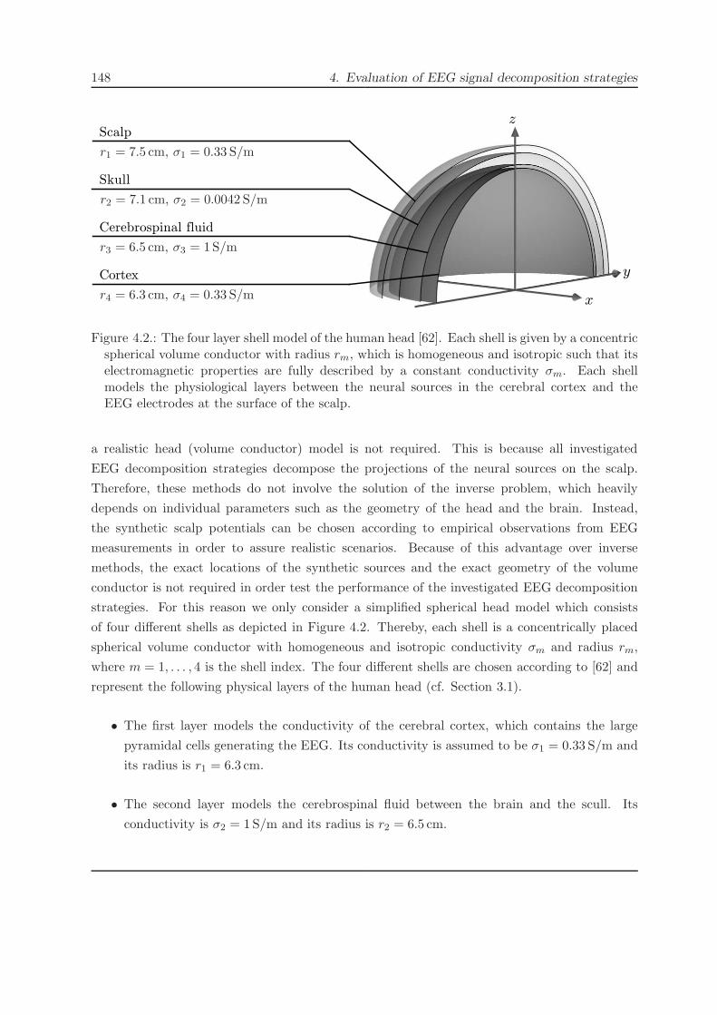
148 4. Evaluation of EEG signal decomposition strategies
!"#$%&'()*+,-./0123456789:;<=>?@ABCDEFGHIJKLMNOPQRSTUVWXYZ[\]_abcdefghijklmnopqrstuvwxyz{|}~
Scalp
x
y
z
Skull
Cerebrospinal fluid
Cortex
r1 = 7.5 cm, σ1 = 0.33 S/m
r2 = 7.1 cm, σ2 = 0.0042 S/m
r3 = 6.5 cm, σ3 = 1S/m
r4 = 6.3 cm, σ4 = 0.33 S/m
Figure 4.2.: The four layer shell model of the human head [62]. Each shell is given by a concentricspherical volume conductor with radius rm, which is homogeneous and isotropic such that itselectromagnetic properties are fully described by a constant conductivity σm. Each shellmodels the physiological layers between the neural sources in the cerebral cortex and theEEG electrodes at the surface of the scalp.
a realistic head (volume conductor) model is not required. This is because all investigated
EEG decomposition strategies decompose the projections of the neural sources on the scalp.
Therefore, these methods do not involve the solution of the inverse problem, which heavily
depends on individual parameters such as the geometry of the head and the brain. Instead,
the synthetic scalp potentials can be chosen according to empirical observations from EEG
measurements in order to assure realistic scenarios. Because of this advantage over inverse
methods, the exact locations of the synthetic sources and the exact geometry of the volume
conductor is not required in order test the performance of the investigated EEG decomposition
strategies. For this reason we only consider a simplified spherical head model which consists
of four different shells as depicted in Figure 4.2. Thereby, each shell is a concentrically placed
spherical volume conductor with homogeneous and isotropic conductivity σm and radius rm,
where m = 1, . . . , 4 is the shell index. The four different shells are chosen according to [62] and
represent the following physical layers of the human head (cf. Section 3.1).
• The first layer models the conductivity of the cerebral cortex, which contains the large
pyramidal cells generating the EEG. Its conductivity is assumed to be σ1 = 0.33 S/m and
its radius is r1 = 6.3 cm.
• The second layer models the cerebrospinal fluid between the brain and the scull. Its
conductivity is σ2 = 1S/m and its radius is r2 = 6.5 cm.

4.1. The generation of synthetic EEG data 149
• The third layer models the conductivity of the scull, which is usually assumed to be 40
to 90 times more restive than the cerebral cortex and the scalp. Here, its conductivity is
σ3 = 0.0042 S/m and its radius is r3 = 7.1 cm.
• The fourth layer models the scalp, whose conductivity is usually similar to the conductivity
of the cerebral cortex. Thus, we assume σ4 = 0.33 S/m and r4 = 7.5 cm.
The parameters of the four shell layers are also summarized in Figure 4.2. For the determination
of the conductivities σm of the different biological materials, the reader is referred to [83]. The
simple geometric nature of the spherical head model according to Figure 4.2 leads to closed-form
solutions for the scalp potentials in case of dipole sources (cf. Section 4.1.4) [63, 123]. These
solutions are computed with the help of the FieldTrip software package [151] throughout this
thesis. Spherical head models with three to four layers have been used extensively in MEG / EEG
source localization applications [159].
4.1.3. EEG electrode setups
Many different systems for the placement of EEG electrodes have been used in literature. Among
those systems we can distinguish between two possible classes of EEG electrode setups covering
the whole cortex, namely the equidistant electrode setups as well as the different electrode
setups which are derived from the international 10-20 system [115]. Furthermore, there are also
specialized electrode setups covering only a specific region of interest on the cerebral cortex.
These setups are therefore specific to certain EEG experiments such as, e.g., the measurement
of early acoustic evoked potentials or visual evoked potentials. Throughout this thesis, we
only consider electrode setups which are derived from the international 10-20 system. The
international 10-20 system as well as the international 10-10 (cf. Figure 4.3) [150] system are
routinely used in many clinical applications. Because of this, also the electrode nomenclature is
defined on the basis of these systems.
4.1.3.1. The 10-20 system and its generalizations
The 10-20 system is the most routinely used EEG electrode setup used in clinical applications
and was introduced in 1958 [115]. The spatial locations of the 21 EEG electrodes included in
this system are depicted in Figure 4.3. For the placement of the electrodes, four reference points
are used, namely the Nasion at the front of the head, the Inion at the back of the head as well
as the preaurical points at the left and right hemisphere of the head. The position of the Cz
electrode is midway on the straight connecting line between the Nasion and the Inion along the

150 4. Evaluation of EEG signal decomposition strategies
!"#$%&'()*+,-./0123456789:;<=>?@ABCDEFGHIJKLMNOPQRSTUVWXYZ[\]_abcdefghijklmnopqrstuvwxyz{|}~
Cz
10%
20%
20%20%
20%10%
10%20%
20%20%
20%
10%
Pz
Fz
A1Inion
Nasion
preaurical point
FP1
F7
T3
A1
T5
O1O2
T6
T4
A2
F8
FP2
Inion
Nasion
Cz
Pz
Fz
C3
P3
C4
P4
F3 F4
FP1
C3
P3
F3
F7T3
T5
F5
F1FC1 C1
CP1
P1
PO
3
P5
CP5
C5FC5
FT7 TP7 PO7
AF7
AF3
AFz
FCz
CPz
PO
z
O1
Oz
FP
z
FC3
CP3
AF7 A
F8
FT
8T
P8
PO8
Oz
PO7
TP
7F
T7
FPzAF3 AFz AF4
F5F1 F2
F8
FC5FC3 FC1 FCz FC2 FC4
FC6
C5 C1 C2 C6
CP5CP3
CP1 CP2CP4
CP6
CPz
P5P1 P2
P6
PO3 POzPO4
Figure 4.3.: The international 10-20 and 10-10 electrode setup for EEG. The lateral view of theleft hemisphere of the head is visualized in the left part, while the top view of the head isdepicted in the right part of the figure. The large circles and rectangles represent the electrodepositions of the 10-20 system. The small circles and rectangles indicate the electrode positionsadditionally included in the 10-10 system.
scalp. Furthermore, Cz (Central zero) is located midway on the connecting line between the two
preaurical points along the scalp. Based on this definition of the location of the Cz electrode
all other electrode positions are found by adding 20% steps, i.e., 20% of the distance between
Nasion and Inion along the scalp for the vertical direction and 20% of the distance between the
two preaurical points along the scalp for the horizontal direction. This definition of the 10-20
system electrode positions is visualized in Figure 4.3.
Because of the limited spatial resolution of the 10-20 system numerous generalizations with
an increased number of electrodes have been defined in literature. Not all of these systems
are standardized and for a full review of all available 10-20 derivates the reader is referred
to [121]. Throughout this thesis, we apply the internationally standardized 10-10 system ac-
cording to [150]. The location of all 61 electrodes included in this version of the 10-10 system is
also depict in Figure 4.3. Thereby, the 10-10 electrode positions are defined in analogy to the
10-20 setup just by considering a 10% step size. Please notice that also other versions of the

4.1. The generation of synthetic EEG data 151
10-10 system have been defined in literature [121] and also additional generalizations, such as the
10-5 setup [152] including a total number of 320 electrodes, have been used for high resolution
EEG applications. However, the spatial resolution of the 10-10 system does suffice for the vast
majority of EEG applications. For the labels of the 10-10 system as depicted in Figure 4.3 the
following rules are applied [150]
• The letters F, P, T, and O indicate the frontal, parietal, temporal, and occipital lobes of
the human brain, respectively.
• The letter C indicates the central region of the human head.
• The label FP (i.e., frontal polar) is used for electrodes at the forehead.
• The letter A indicates an earlobe reference electrode.
• All electrodes placed on the left hemisphere of the head are labeled with odd numbers,
while all electrodes placed on the right hemisphere are labeled with even numbers.
• For electrodes on the edge between the left and right hemisphere the electrode number is
replaced by z (i.e., zero).
• The labels for electrodes with the intermediate locations of the 10-10 system are AF
(midway FP and F), FC (midway F and C), CP (midway C and P), TP (midway T and
P), and PO (midway P and O).
4.1.4. The EEG source model
For our investigations based on synthetic EEG, we generally assume that the scalp potentials are
generated by equivalent current dipoles. Thereby, a current dipole represents the simultaneous
and coherent activation of a large number of pyramidal cells within a small patch of possibly
some square centimeters within the cerebral cortex. If larger areas of the cerebral cortex are
simultaneously activated (distributed sources), these areas can be divided into smaller regions
each represented by a single current dipole. These regions are termed the macro-columns of
the cerebral cortex (cf. Section 3.1). In general, the current dipole represents an adequate
approximation of the activated cortical macro-columns if their generated potentials are observed
at some distance on the scalp. The current dipole is the standard model for neural sources used
routinely in EEG / MEG signal processing [174] and medical imaging techniques [29]. Other
source models, such as the multipolar source [145], are only rarely used in literature. Every
current dipole is fully described by its position pr and the dipole moment xr(t). Thereby, the
dipole moment is given by the direction mr(t) and the dipole signal sr(t) with xr(t) = mr(t) ·

152 4. Evaluation of EEG signal decomposition strategies
sr(t). Since EEG is mainly generated from radial sources (cf. Section 3.1), we generally assume
a radial direction of the dipole sources, i.e., mr(t) is perpendicular to the surface of the shells of
the volume conductor model (cf. Section 4.1.2). In the following, we make a distinction between
static dipoles with fixed location and direction, and dynamic dipoles modeling a virtually moving
neural source [171].
4.1.4.1. Static EEG sources
With the help of static dipoles, we model neural sources with a constant location within a certain
time window. As a consequence, the scalp potentials of these static sources vary over time only
by the dipole signals sr(t). The spatial weights, and therewith the leadfield matrix L in the
forward model (4.7), remain constant. Each of the R static dipole sources are fully described
by the constant spatial positions pr within the volume conductor and the constant unit-norm
dipole directions mr for r = 1, . . . , R. As mentioned above, the dipole directions mr are chosen
to be radial, i.e., mr points in the same direction as pr and is perpendicular the surface of
the volume conductor shells. An example of a static dipole source is depicted in Figure 4.4a.
The dipole is located underneath the lowest shell of the volume conductor, which represents the
cerebral cortex. The vector pr with the cartesian coordinates of the r-th dipole source can also
be represented in spherical coordinates, i.e., the radius ℓr = ∥pr∥F, the azimuth angle φr and
the elevation angle θr or the co-elevation angle ϑr = π2 − θr. Thereby, the relations between
cartesian and spherical coordinates are given by
ℓ =√
x2 + y2 + z2 x = ℓ sinϑ cosφ
φ = arctan2 (x, y) =
⎧⎪⎪⎪⎪⎪⎪⎪⎪⎪⎨
⎪⎪⎪⎪⎪⎪⎪⎪⎪⎩
arctan yx for x > 0
arctan yx + π for x < 0, y ≥ 0
arctan yx − π for x < 0, y < 0
π2 for x = 0, y > 0
−π2 for x = 0, y < 0
0 for x = 0, y = 0
y = ℓ sinϑ sinφ
ϑ = arccos(zℓ
)z = ℓ cos ϑ .
(4.8)
In general, the radius ∥pr∥F of the dipole sources is chosen to be between 2mm (radial source
in the gyri) and 1.3 cm (radial source at the bottom of the sulci) below the radius of the shell
modeling the cerebral cortex, which has a radius of 6.3 cm (cf. Figure 4.2). An example for
simulated EEG generated by a single static radial source located 3mm underneath the parietal-
occipital electrode PO4 (cf. Section 4.1.3) is depicted in Figure 4.5. Here, the dipole signal

4.1. The generation of synthetic EEG data 153
!"#$%&'()*+,-./0123456789:;<=>?@ABCDEFGHIJKLMNOPQRSTUVWXYZ[\]_abcdefghijklmnopqrstuvwxyz{|}~
a)
xy
z
xy
z
b)
dipole trajectory
mr
φr
θr
pr
mr(t)
pr(t)
ϑr
Figure 4.4.: The static and dynamic source model for EEG in Figure a) and Figure b), respec-tively. In both cases the dipoles are located closely underneath the surface of the inner shellof the volume conductor. In case of the static sources in Figure a, the dipole position pr aswell as the dipole direction mr are fixed. The dipole position is equivalently described bythe spherical coordinates with the radius ℓr, the azimuth angle φr the elevation angle θr orthe co-elevation angle ϑr. In case of the dynamic sources in Figure b, a virtual movement ofthe neural source is simulated by multiple dipoles along a radial trajectory pr(t), which areactivated consecutively in time. For both static and dynamic dipoles the direction mr(t) ischosen to be perpendicular to the shell surface (radial sources).
s1(t) follows the typical course of a measured evoked potential and is generated according to
Table 4.1. The spatial distribution (weights) of this source is depicted in the topographic plot in
the left upper part of Figure 4.5. A clear and strongly focal activation is observed directly in the
area around the PO4 electrode. In the right part of the same figure, we show the sensor signals
of all the EEG sensors of the international 10-10 system [150] located in the lower hemisphere
of the head. As we can see, the different sensor signals y(t) follow the exact shape of the dipole
signal s1(t) and differ from channel to channel only by the scalar spatial weights presented in the
topographic plot of the source. In Table 4.1 we present typical dipole signals together with their
corresponding mathematical representation and their temporal course. Thereby, the parameters
of the dipole signals are chosen according to observations made in typical EEG measurements.
Please notice that the exact temporal location of the signals is not parameterized within the
corresponding equations for the dipole signals.

154 4. Evaluation of EEG signal decomposition strategies
!"#$%&'()*+,-./0123456789:;<=>?@ABCDEFGHIJKLMNOPQRSTUVWXYZ[\]^_`abcdefghijklmnopqrstuvwxyz{|}~
0.03
0.025
0.02
0.015
0.01
0.005
0
-0.005
0 0.1 0.2 0.3 0.4 0.5
1
0.5 t0 0.25
time in seconds time in seconds
O2OzO1
PO8PO4POzPO3PO7T6P6P4P2PzP1P3P5T5
TP8CP6CP4CP2CPzCP1CP3CP5TP7
sr(t)
Figure 4.5.: An example of a static radial dipole source for EEG located directly underneaththe parietal-occipital PO4 electrode. In the upper left part we depict the topography of thespatial weights generated by this source. Furthermore, the dipole signal sr(t) is plotted in thelower left part. In the right part of the figure, we show the resulting sensor signals sr(t) forall EEG channels in the lower hemisphere of the head.
4.1.4.2. Dynamic EEG sources
As already mentioned in Section 3.3.3, temporally shifted evoked potentials are often observed
in measured EEG as for example visualized in Figure 3.7 for the case of measured Visual Evoked
Potentials (VEP). For this case, the peak latencies of the VEP differ from channel to channel
and therefore depend on the spatial location of the electrode on the scalp. In general, the
electrodes at the visual cortex show the lowest peak latencies. Hence, the visual cortex is
responding first to the visual stimulus (cf. Figure 3.7b). The fact that the shape of the evoked
potentials is approximately constant, and therefore vary from channel to channel only by a
scalar value and a temporal shift, indicates the presence of a virtually moving EEG source.
Thereby, a spatial movement of the scalp potentials is observed because neighboring patches
(macro-columns) in the cerebral cortex are activated consecutively in time. This spatial drift of
the scalp potentials can be modeled with the help of a virtually moving dipole source [171–173]
in the forward solution (4.7). Thereby, the dipole is moving along the trajectory p(t) as depicted
in Figure 4.4b. For these dynamic EEG sources, we generally assume a circular trajectory with
a constant radius ∥p(t)∥F and constant distance to the surface of the lowest shell of the volume

4.1. The generation of synthetic EEG data 155
Signal Type Equation Time course
alpha waves(t) = sin(2πft)frequency f = 10Hz
!"#$%&'()*+,-./0123456789:;<=>?@ABCDEFGHIJKLMNOPQRSTUVWXYZ[\]_abcdefghijklmnopqrstuvwxyz{|}~
1
1
-1
s(t)
t
modulatedalpha wave
s(t) = e−t2
σ2 · cos(2πft)variance σ2 = 0.05 s2
frequency f = 10Hz
!"#$%&'()*+,-./0123456789:;<=>?@ABCDEFGHIJKLMNOPQRSTUVWXYZ[\]_abcdefghijklmnopqrstuvwxyz{|}~
1
1
-1
s(t)
t
sharp triangularspike
s(t) =
{1− | tT | ∀ −
T2 ≤ t ≤ T
20 else
duration T = 0.05 s
!"#$%&'()*+,-./0123456789:;<=>?@ABCDEFGHIJKLMNOPQRSTUVWXYZ[\]_abcdefghijklmnopqrstuvwxyz{|}~
1
1s(t)
t
slow spikes(t) =
{1− t2
T 2 ∀ − T2 ≤ t ≤ T
20 else
duration T =√0.05 s
!"#$%&'()*+,-./0123456789:;<=>?@ABCDEFGHIJKLMNOPQRSTUVWXYZ[\]_abcdefghijklmnopqrstuvwxyz{|}~
1
1s(t)
t
evoked poten-tial
s(t) =
{e−
tT · sin(2πft) t ≥ 0
0 elsefrequency f = 4Hzduration T = 0.05 s
!"#$%&'()*+,-./0123456789:;<=>?@ABCDEFGHIJKLMNOPQRSTUVWXYZ[\]_abcdefghijklmnopqrstuvwxyz{|}~
1
1s(t)
t
Table 4.1.: Overview of possible dipole signals used for the generation of synthetic EEG data.The parameters shown here are only exemplary and might be adapted. Please notice that thetime courses depicted in the third row only show the shape of the dipole signals. The exactlocation of the signals on the time axis is not parameterized in the respective equations in thesecond row.
conductor model. Therefore, the trajectory shows a constant co-elevation angle ϑr, a constant
radius ℓr = ∥pr(t)∥F and a time-varying azimuth angle
φr(t) = ωr · t+ φr,0 , (4.9)
where φr,0 is the azimuth angle at the time instant t = 0 and ωr is the angle-velocity of the
r-th moving dipole source with r = 1, . . . , R. With the help of the relations (4.8) the dipole

156 4. Evaluation of EEG signal decomposition strategies
trajectory pr(t) is given in cartesian coordinates by
pr(t) =
⎛
⎜⎝px,r(t)
py,r(t)
pz,r(t)
⎞
⎟⎠ =
⎛
⎜⎝ℓr · sinϑr · cos (ωr · t+ φr,0)
ℓr · sinϑr · sin (ωr · t+ φr,0)
ℓr · cos ϑr
⎞
⎟⎠ . (4.10)
Since every EEG source has to be located in the northern hemisphere of the volume conductor
shells, the co-elevation angle ϑr of each source has to be chosen within the range ϑr = 0, . . . , π2 .
Furthermore, the radius ℓr is chosen in the range of ℓr = 5, . . . , 6 cm, similarly to the static
sources. Since we only consider EEG which is mainly generated from radial sources (cf. Sec-
tion 3.1), the direction mr(t) of the dipole along its trajectory pr(t) is chosen to be perpendicular
to the surface of the shells of the volume conductor model. Therefore, the vector mr(t) is always
parallel to the dipole position vector pr(t) and is restricted to have unit norm, such that
mr(t) =
⎛
⎜⎝mx,r(t)
my,r(t)
mz,r(t)
⎞
⎟⎠ =
⎛
⎜⎝sinϑr · cos (ωr · t+ φr,0)
sinϑr · sin (ωr · t+ φr,0)
cos ϑr
⎞
⎟⎠ . (4.11)
In order to implement the virtually moving dipole within the forward model (4.7), we use the
following procedure [7]. For every time-instant t of the dipole signal sr(t) we determine the
corresponding dipole position pr(t) according to (4.10) on the dipole trajectory together with
the corresponding radial dipole directionm(t) according to (4.11). In the sequel, we compute the
corresponding leadfield matrix Lr(t) from the parameters pr(t) and m(t) for the corresponding
time-instant t using the FieldTrip software package [151]. As a consequence, we obtain a time-
varying leadfield matrix Lr(t) for the r-th dynamic dipole source, such that the complete forward
model (4.7) reads as
y(t) = L(t) · vec (M(t) · diag (s(t))) + e(t) . (4.12)
Please notice that this way of modeling virtually moving neural sources exactly emulates the
physiological reason for the spatial drift of the scalp potentials. This physiological reason is of
course not given by a physical movement of a neural source within the cerebral cortex, but by
the temporally sequential activation of neighboring patches (macro-columns) in the cortex. In
Figure 4.6, we present an example for the EEG sensor signals generated by one dynamic radial
dipole source. Thereby, the dipole models a virtually moving neural activation starting at the
parietal P3 electrode in the left hemisphere and following a circular trajectory with constant
radius to the parietal P4 electrode in the right hemisphere of the head. The resulting time-variant
topography is depicted for four equally spaced snapshots in the upper left part of Figure 4.6.
The spatial drift of the focal activation of the radial source from the P3 to the P4 electrode is

4.1. The generation of synthetic EEG data 157
!"#$%&'()*+,-./0123456789:;<=>?@ABCDEFGHIJKLMNOPQRSTUVWXYZ[\]^_`abcdefghijklmnopqrstuvwxyz{|}~
0 0.1 0.2 0.3 0.4O2OzO1
PO8PO4POzPO3PO7T6P6P4P2PzP1P3P5T5
TP8CP6CP4CP2CPzCP1CP3CP5TP7
0 0.40.2 t
1
time in secondstime in seconds
0 ms 133 ms
266 ms 400 ms
0.03
0.025
0.02
0.015
0.01
0.005
0
-0.005sr(t)
Figure 4.6.: An example of a dynamic radial dipole source for EEG, which simulates a virtualmotion starting at the parietal P3 electrode moving towards the parietal P4 electrode asvisualized by the topographic snapshots in the left upper part of this figure. In the left lowerpart we depict the signal transmitted by the moving dipole. On the right side we show theresulting sensor signals, which show a clear shift in their peak latencies.
clearly visible. The dipole source signal used for this simulation is depicted in the lower left part
of the same figure and is generated as a Gaussian modulated wave according to Table 4.1 with
the empirical parameters f = 4Hz and σ2 = 0.005 s2. The resulting sensor signals are presented
on the right part of Figure 4.6 for all electrodes of the international 10-10 system located in the
lower hemisphere of the head. As we can see, the sensor signals differ not only by a scalar value
from channel to channel. Instead their peak latencies vary in dependency to the sensor position.
The shape of the sensor signals is approximately equal. However, it has to be noticed that the
shape of the sensor signals does not exactly correspond to the shape of the dipole signal sr(t).
This is because the time-varying leadfield matrix L(t) introduces an additional time dependent
deformation to the source signals.
4.1.5. The consideration of realistic noise (background EEG)
As already mentioned in the introduction of Section 4.1, we also consider realistic background
EEG for the generation of synthetic EEG data. Thereby, the background EEG is caused by
unspecific neural activity observed in all EEG measurements and is represented by the additive
noise term e(t) in the forward model (4.7). In order to model the noise term e(t) as realistic as

158 4. Evaluation of EEG signal decomposition strategies
possible we estimate its parameters based on measured EEG.
To achieve this, we record background EEG from a 23 year old, healthy and male test person.
In order to assure that the EEG data are mainly caused by unspecific neural activity, the test
person was placed in front of a white wall and was not performing any tasks. To reduce the
generation of alpha activity in the occipital region of the head (which is observed for the most
test persons when they close their eyes) the test person left its eyes open. The measurement
duration is set to 10 minutes and the standard 10-10 electrode system (cf. Figure 4.3) was used.
The sampling frequency is 512Hz and the Common Average Reference (CAR) is used for the
measurements.
For the rejection of artifacts in the measured background EEG, the following preprocessing is
applied (cf. Section 4.3.1). First, the following linear time-invariant filters are applied to the
measured background EEG in order to extract the frequency range of interest
• a 4-th order butterworth highpass filter with a cut-off frequency of 0.1Hz;
• a 4-th order butterworth lowpass filter with a cut-off frequency of 100Hz;
• a 50Hz notch filter.
All filters are applied in forward and reverse direction in order to achieve zero phase distortions.
After these filters are applied to the measured EEG signals, the ICA is used in order to remove
eye-blink artifacts (cf. Section 3.3.1). Eye-blink artifacts usually appear coherently in all EEG
channels and a very large number of time samples is available in these EEG measurements.
In such situations, the ICA usually shows a very good performance in the extraction of the
eye-blink artifacts [72].
In order to characterize the properties of the measured background EEG, we estimate the Power
Spectral Density (PSD) and the amplitude Probability Density Function (PDF) over all time
samples and EEG channels. The results are depicted in Figure 4.7. The PSD in Figure 4.7a
is estimated using the Welch method [210] with a Hamming window of 5 s duration and an
overlap of 50%. It is easily recognized that the spectral characteristics of the background EEG
follows a constant descend of -10 dB per decade. This is also shown by the first order regression
polynomial, which is fitted to the estimated Welch PSD and is depicted by a gray dashed line
in the same figure. Please notice that the strong drop in the PSD at 50Hz is due to the above
mentioned notch filter applied during the preprocessing of the data. The amplitude PDF of the
measured background EEG is depicted in Figure 4.7b and shows a Gaussian distribution. In
conclusion, the background EEG can be modeled as Gaussian noise with 1/f PSD characteristic

4.1. The generation of synthetic EEG data 159
!"#$%&'()*+,-./0123456789:;<=>?@ABCDEFGHIJKLMNOPQRSTUVWXYZ[\]^_`abcdefghijklmnopqrstuvwxyz{|}~
a) b)
50403020100-10-20-30-40-500
0.01
0.02
0.03
0.04
0.05
0.06
0.07
0.08
-40
-35
-30
-25
-20
-15
-10
0
-5
10
5
10 1010 10-1 0 1 2
frequency f in Hz EEG amplitude in µV
−9.3450 − 10.0039 · log(f)
pow
er/frequ
ency
indB/H
z
probab
ilityden
sity
Figure 4.7.: The estimated characteristics of measured background EEG. In Figure a, the PowerSpectral Density (PSD) estimated using Welchs method is shown [7]. It is characterized by anearly constant descent of -10 dB per decade. This is also shown by the gray dashed line whichrepresents the least squares fit of a first order polynomial to the estimated PSD. Figure bshows the estimated amplitude PDF of the background EEG following a Gaussian distribution.
(power law noise). For the computational method of generating this power law noise with the
help of digital filters, the reader is referred to [122].
In order to proof that the measured background EEG is mainly caused by unspecific neural
activity, we also investigate the spatial correlation of the measured EEG channels. This is
necessary since the noise generated by EEG amplifiers also obeys a Gaussian PDF with a 1/f
power law characteristic [107]. For this analysis, we investigate the topography of the Pearson
correlation coefficients between a certain reference channel and all other measured EEG channels.
This correlation topography is depicted in Figure 4.8 for the exemplary reference channels Cz and
Oz. From these topographies, we can conclude that the measured EEG channels are spatially
correlated only to their neighboring EEG channels. This is a strong indication that the measured
signals are not mainly generated from the spatially uncorrelated amplifier noise. Instead they
represent the spatially correlated electric field potentials at the surface of the scalp measured by
the EEG electrodes.

160 4. Evaluation of EEG signal decomposition strategies
!"#$%&'()*+,-./0123456789:;<=>?@ABCDEFGHIJKLMNOPQRSTUVWXYZ[\]_abcdefghijklmnopqrstuvwxyz{|}~
Cz1
0.5
0
-0.5
a) b)
Oz
Pea
rson
cor
rele
atio
n c
oeffic
ient
Figure 4.8.: The topographic spatial correlation analysis for the measured background EEG.In Figure a we show the topography of the Pearson correlation coefficient between the Czelectrode and all other EEG electrodes. Equivalently, Figure b shows topography of thecorrelation to the Oz electrode. Both examples show that the measured EEG channels arecorrelated only to their neighboring electrodes.
4.2. Comparative performance assessment of EEG decomposition
strategies based on simulated data
In this section, we investigate and compare the performance of the different EEG decomposition
strategies discussed in Chapter 3 based on simulated EEG data. Thereby, we use the techniques
and definitions described in Section 4.1 for the generation of synthetic EEG. Please note that an
objective and quantifiable performance assessment for all EEG decomposition strategies requires
the usage of simulated EEG data, since all the parameters of the underlying neural sources have
to be known exactly. This is generally not the case for measured EEG data.
For a direct comparison of the estimated sources (computed with the different EEG decomposi-
tion strategies) to the simulated EEG sources, we have to identify a source representation which
is compatible with all EEG decomposition strategies. Since the 3D PARAFAC and PARAFAC2
based strategies utilize a space-time-frequency representation of the EEG sources (cf. Sec-
tion 3.3.3 and 3.3.2), we have to transform both the original synthetic EEG sources, as well as
the estimated sources computed by the ICA based decomposition strategy, to their corresponding
space-time-frequency representations. This is possible by performing a Time-Frequency Analysis
(cf. Section 3.4) on every channel of the original synthetic sources and the estimated ICA com-
ponents (see Figure 4.9). Once all neural sources are transformed to their space-time-frequency

4.2. Comparative performance assessment of EEG decomposition strategies based on
simulated data161
!"#$%&'()*+,-./0123456789:;<=>?@ABCDEFGHIJKLMNOPQRSTUVWXYZ[\]_abcdefghijklmnopqrstuvwxyz{|}~
Synthetic EEG
ICA Decomposition
Strategy
PARAFAC / PARAFAC2 Decomposition Strategy
Time-Frequency Analysis
Time-Frequency Analysis
Reference Sources
Estimated Sources
Estimated Sources
Com
pari
son
y(t) = y1(t) + y2(t) + e(t)
y1(t)
y2(t) Y1, Y2
y(t)y1(t)
y2(t) Y1, Y2
y(t)
Y1, Y2
Figure 4.9.: Method for the comparison of the different EEG decomposition strategies based onsimulated EEG data. Since the quadratic Time-Frequency Analysis (TFA) methods utilizedin the PARAFAC and PARAFAC2 based decomposition strategy are not invertible, all sourceshave to be compared using their space-time-frequency representation. Therefore, a TFA hasto be performed on every channel of the simulated reference sources as well as on the estimatedICA sources.
representation, an objective comparison between all EEG decomposition strategies is possible
by using the original simulated sources as a reference. This method of comparing the different
EEG decomposition strategies is visualized in Figure 4.9 for a two-source problem. Please note
that a direct comparison is only possible based on the space-time-frequency representation of
the sources, since the quadratic TFA methods used throughout this thesis are not invertible.
For the comparison of the estimated sources to the reference sources we define the following
four possible measures. The normalized source Mean Squared Error (MSE) eS between the full
space-time-frequency representations of the reference sources Yr and the estimated sources Yr
is given by
eS =∥Yr −Yr∥2H∥Yr∥2H
. (4.13)
Here, r = 1, . . . , R is the component index, where R is the total number of neural sources.
Furthermore, we measure the similarity between the estimated sources Yr and the reference

162 4. Evaluation of EEG signal decomposition strategies
sources Yr using the source correlation pS by computing the Pearson correlation coefficient
pS =
(vec
(Yr
)−mean
(Yr
))T·(vec
(Yr
)−mean
(Yr
))
∥∥∥(vec
(Yr
)−mean
(Yr
))∥∥∥F·∥∥∥(vec
(Yr
)−mean
(Yr
))∥∥∥F
. (4.14)
Since the topographic analysis of the neural sources is one of the key goals of the EEG decompo-
sition strategies discussed throughout this thesis, we also focus on the normalized topographic
MSE eT computed by
eT =
∥∥∥ cr∥cr∥F −
Lr ·mr
∥Lr ·mr∥F
∥∥∥2
F
∥Lr ·mr∥2F. (4.15)
Here, cr represents the channel signature of the r-th estimated component and Lr ·mr is the
vector of channel weights of the r-th simulated source (cf. equation (4.5)). In case of the ICA
decomposition strategy, cr corresponds to the r-th column of the ICA mixing matrix (cf. equa-
tion (3.2)). In case of the PARAFAC and PARAFAC2 decomposition strategy, cr corresponds
to the channel signature of the r-th estimated component (cf. equation (3.4) and (3.9)). Fur-
thermore, we also focus on the topography correlation pT by computing the Pearson correlation
coefficient
pT =
(cr −mean
(cr))T
·(Lr ·mr −mean
(Lr ·mr
))
∥∥∥(cr −mean
(cr))∥∥∥
F·∥∥∥(Lr ·mr −mean
(Lr ·mr
))∥∥∥F
. (4.16)
In the following sections, we investigate the performance of the different EEG decomposition
strategies based on static sources with constant channel weights (cf. Section 4.1.4.1) and dy-
namic sources with time-varying channel weights (cf. Section 4.1.4.2). Thereby, we compare the
3D PARAFAC based decomposition strategy against the 2D ICA based decomposition strat-
egy for static sources in Section 4.2.1. Please note that we do not explicitly investigate the
PARAFAC2 based decomposition strategy for static sources, since the PARAFAC2 model re-
duces to PARAFAC in this case. The dynamic sources are investigated in Section 4.2.2. Here,
we proof that only the PARAFAC2 based decomposition strategy is capable to reconstruct the
time-varying channel weights of dynamic sources.
4.2.1. Assessments based on static EEG sources
In order to proof the superior performance of the 3D PARAFAC and PARAFAC2 based decom-
position strategy over the 2D ICA based decomposition strategy, we compare both decompo-
sition methods based on static EEG sources. Thereby, static EEG sources are used to model

4.2. Comparative performance assessment of EEG decomposition strategies based on
simulated data163
!"#$%&'()*+,-./0123456789:;<=>?@ABCDEFGHIJKLMNOPQRSTUVWXYZ[\]^_`abcdefghijklmnopqrstuvwxyz{|}~
1
SNR in dB
sourc
e co
rrel
ation
time in seconds
0.5 t0 0.25
PARAFACJADE ICA
FastICAProKRaft ICA
0.03
0.025
0.02
0.015
0.01
0.005
0
-0.005
40200-20-400
0.1
0.2
0.3
0.4
0.5
0.6
0.7
0.8
0.9
1
sr(t)
Figure 4.10.: The source correlation pS according to (4.14) for one static dipole source. Thereby,pS is averaged over 100 realizations and is depicted for varying SNRs on the right part ofthe figure. The left part shows the topography of the channel weights as well as the signaltransmitted by the dipole source. Thereby, the dipole is located directly underneath the Pzelectrode with a radial orientation and a radius of 6 cm.
typical activations in the cerebral cortex with constant spatial location. Therefore, the topo-
graphic scalp projections of these sources remain constant over time (cf. Section 4.1.4.1). In
the following, we investigate the single source problem in order to proof that the considered
decomposition strategies are capable to model typical static EEG sources. Thereby, we consider
different source signals found in typical EEG measurements (cf. Table 4.1) as well as different
TFA methods (cf. Section 3.4). Comparable simulations with two different static EEG sources
are carried out in Section 4.2.1.2. Please note that we do not explicitly simulate the PARAFAC2
based decomposition strategy here, since the PARAFAC2 model is theoretically equivalent to
the PARAFAC model for the case of static EEG sources.
4.2.1.1. The single source problem
In this section, we address the problem of identifying the single, dominant, static EEG source
from the synthetic EEG data. In order to achieve this, we place a single radial dipole with
a radius of 6 cm at the occipital region of the head, directly underneath the Pz electrode (cf.
Figure 4.3). The topographic projection of this source is depicted in the upper left part of
Figure 4.10. In our first simulations, we consider a dipole signal s(t) which follows the typical

164 4. Evaluation of EEG signal decomposition strategies
time course of Evoked Potentials (EP) as depicted in the lower left part of Figure 4.10. In
general, we consider additive power law noise with a 1/f frequency characteristic and Gaussian
Probability Density Function (PDF) (cf. Section 4.1.5) in order to model unspecific background
EEG activity. Thereby, the Signal-to-noise Ratio (SNR) in dB is generally defined by
SNR = 10 · log10Ps(t)
Pe(t), (4.17)
where Ps(t) is the total power of the source signal and Pe(t) is the total noise power. In the right
part of Figure 4.10 we present the source correlation pS according to equation (4.14) between the
estimated dominant source and the simulated reference source over varying SNRs. This source
correlation is averaged over 100 trials. Thereby, we consider the PARAFAC decomposition
strategy using the HOOI method (cf. Section 2.2.3.4) for the computation of the dominant rank-
one source as well as the ICA based decomposition strategy using three different ICA algorithms.
The three ICA algorithms are the JADE algorithm according to [44, 46], the ProKRaft ICA
Algorithm 8, as well as the FastICA algorithm according to [110,111]. Please notice that it is not
possible to estimate only one source in a multi-channel signal using the ICA, since the assumption
of mutual independence between the sources requires at least two different sources. Therefore,
we identify the dominant EEG source in this simulation by estimating two independent sources.
One of these sources models the dipole source according to Figure 4.10, while the second source
models the noise. Finally, we select the ICA source with maximum source correlation pS. In
contrast to this, it is possible to identify the dominant neural source directly using the PARAFAC
based decomposition strategy. For the Time-Frequency Analysis (TFA) we used the RID with a
truncated Choi-Williams kernel (also termed Exponential Distribution (ED), cf. Section 3.4.2).
The sampling frequency for the source signal is chosen to be 1000Hz. From the simulation
shown in the right part of Figure 4.10 we can conclude that all ICA algorithms show a similar
performance. Only the ProKRaft ICA algorithm shows a slightly worse performance in the
SNR range of -10 dB to 10 dB, which is due to the estimation error in the fourth order cumulant
tensor (cf. Section 2.3.3.3). The PARAFAC decomposition strategy performs slightly better than
the ICA based decomposition strategy in the static single source case. These results are also
confirmed by the topography MSE eT and the topography correlation pT depicted in Figure 4.11
for this simulation scenario. Again, both eT and pT are averaged over 100 realizations.
In order to compare the ICA and PARAFAC based decomposition strategy also for other source
signals s(t) as well as for other TFA methods, we select the topography correlation pT according
to equation (4.16) as a performance measure. This measure is of particular interest, since the
topographic analysis of the EEG sources is one of the most important applications of all EEG

4.2. Comparative performance assessment of EEG decomposition strategies based on
simulated data165
!"#$%&'()*+,-./0123456789:;<=>?@ABCDEFGHIJKLMNOPQRSTUVWXYZ[\]^_`abcdefghijklmnopqrstuvwxyz{|}~
SNR in dB
topogra
phy c
orr
elation
PARAFACJADE ICA
FastICAProKRaft ICA
40200-20-40
0.1
0.2
0.3
0.4
0.5
0.6
0.7
0.8
0.9
1.0
0
PARAFACJADE ICA
FastICAProKRaft ICA
SNR in dB
topogra
phy r
econst
ruct
ion e
rror
40200-20-40
0.1
0.2
0.3
0.4
0.5
0.6
0
Figure 4.11.: The topography reconstruction error eT according to (4.15) and the topographycorrelation pT according to (4.16) for the static dipole source presented in Figure 4.10. Alldisplayed values of eT and pT are averaged over 100 trials.
decomposition strategies. Thereby, we define the threshold SNR as the SNR in dB at which
the topography correlation pT exceeds a value of 0.9. In Table 4.2, we show this threshold SNR
for different combinations of source signals s(t) and TFA methods for both the ICA and the
PARAFAC based decomposition strategy. Since the JADE algorithm usually outperforms the
RID PWVD SPWVD CWT
EP PARAFAC: -10.2 dB,ICA: -5.6 dB
PARAFAC: -10.1 dB,ICA: -5.6 dB
PARAFAC: -11.1 dB,ICA: -5.6 dB
PARAFAC: -9.6 dB,ICA: -5.6 dB
CW PARAFAC: -10.1 dB,ICA: -7.6 dB
PARAFAC: -10.4 dB,ICA: -7.6 dB
PARAFAC: -10.5 dB,ICA: -7.6 dB
PARAFAC: -11.2 dB,ICA: -7.6 dB
MW PARAFAC: -10.9 dB,ICA: 0.0 dB
PARAFAC: -11.4 dB,ICA: 0.0 dB
PARAFAC: -11.7 dB,ICA: 0.0 dB
PARAFAC: -11.1 dB,ICA: 0.0 dB
SP PARAFAC: -10.8 dB,ICA: -5.9 dB
PARAFAC: -10.5 dB,ICA: -5.9 dB
PARAFAC: -11.9 dB,ICA: -5.9 dB
PARAFAC: -10.7 dB,ICA: -5.9 dB
Table 4.2.: The 0.9 topography correlation threshold SNR for the static dipole source as depictedin Figure 4.10. For the computation of the ICA we use JADE. The abbreviations, signalparameters and TFA parameters are given in the text. All values are averaged over 100realizations.
other ICA algorithms in the scenarios investigated throughout this thesis, we always use JADE
for the computation of the ICA based decomposition strategy in the following simulations. In
Table 4.2 we used the following source signal abbreviations and parameters

166 4. Evaluation of EEG signal decomposition strategies
• The Evoked Potentials (EP) with frequency f = 4Hz and duration T = 0.05 s.
• The Continuous Wave (CW) with frequency f = 10Hz.
• The Modulated Wave (MW) with frequency f = 10Hz and variance σ2 = 0.05 s2.
• The Slow Spike (SP) with duration T =√0.05 s.
The time courses and mathematical formulations of these source signals are given in Table 4.1.
For the different TFA methods we used the following empirically chosen parameters
• The Pseudo Wigner-Ville Distribution (PWVD) with a hamming window h(t) of 128 sam-
ples.
• The Smoothed Pseudo Wigner-Ville Distribution (SPWVD) with a hamming window h(t)
of 128 samples and a boxcar window g(t) of 21 samples.
• The Reduced Interference Distribution (RID) using a truncated Choi-Williams kernel, also
termed Exponential Distribution (ED).
• The Continuous Wavelet Transform (CWT) using a complex Morlet Wavelet with a band-
width of fB = 0.5Hz and a center frequency of fC = 0.25Hz.
For more information about the different TFA methods and their parameters the reader is
referred to Section 3.4. From the threshold SNR values in Table 4.2 we can conclude that
the PARAFAC based decomposition strategy always outperforms the ICA based decomposition
strategy. Furthermore, the PARAFAC based decomposition strategy produces almost constant
threshold SNRs from -10 dB to -11 dB for all considered source signals. This is in contrast
to the ICA based decomposition strategy which performs particularly bad in case of a MW
dipole signal. These simulations confirm the theoretical advantages of the PARAFAC based
decomposition strategy over the ICA based decomposition strategy discussed in Chapter 3.
Please note that besides the good results for the CWT shown in Table 4.2, this TFA method is
not suited for CW, MW, and SP dipole signals. The reason for this is that the source correlation
pS according to equation (4.14) does not converge to one for these signals.
Non-stationary sources As already mentioned in the theoretical description of the ICA based
decomposition strategy (cf. Section 3.3.1), the ICA assumes stationary and mutually indepen-
dent source signals. However, there is no physiological justification for these two assumptions in
case of EEG. In order to investigate a scenario where these assumptions are violated, we choose
the MW dipole signal which represents a sine-wave with time-varying amplitude (cf. Table 4.1).
The fact that the ICA based decomposition strategy performs worse for such non-stationary

4.2. Comparative performance assessment of EEG decomposition strategies based on
simulated data167
!"#$%&'()*+,-./0123456789:;<=>?@ABCDEFGHIJKLMNOPQRSTUVWXYZ[\]^_`abcdefghijklmnopqrstuvwxyz{|}~
SNR in dB
sourc
e co
rrel
ation
PARAFACJADE ICA
FastICAProKRaft ICA
40200-20-400
0.1
0.2
0.3
0.4
0.5
0.6
0.7
0.8
0.9
1.0
SNR in dB
topogra
phy c
orr
elation
PARAFACJADE ICA
FastICAProKRaft ICA
40200-20-400
0.1
0.2
0.3
0.4
0.5
0.6
0.7
0.8
0.9
1.0
Figure 4.12.: The source correlation pS and the topography correlation pT for one non-stationarystatic source including correlated noise. The source location and orientation are the same asin Figure 4.10. The dipole transmitted a MW signal with frequency f = 10Hz and varianceσ2 = 0.05 s2. For the TFA we used the ED. All values are averaged over 100 trials. The ICAbased approaches fail to identify the source correctly since pS does not converge to one.
signals is already observed for the threshold SNRs simulations presented in Table 4.2. Please
note that the term non-stationary is used here in order to describe the fact that certain signal
parameters, such as the amplitude of the MW signal, change over time. In order to create an
additional dependency between the dipole signal and the power-law noise eP(t), we scale the
instantaneous power of the noise with the instantaneous amplitude of the MW dipole signal,
such that e(t) = eP(t) · e−(t−0.25)2
σ2 . The parameter σ is chosen again according to the parameters
of the MW signal in Table 4.1. The results for this scenario are depicted in Figure 4.12 for
both the ICA and the PARAFAC based decomposition strategy. Thereby, we present the source
correlation pS and the topography correlation pT over varying SNRs. For the TFA we choose
the RID using a truncated Choi-Williams kernel. It is easily recognized that the ICA based
decomposition strategy cannot identify the underlying neural source signal. This is reflected by
the fact that the source correlation pS does not converge to one in this scenario. In contrast
to this, the PARAFAC based decomposition strategy is not affected by non-stationary sources
with time-varying amplitudes and source-dependent noise characteristics.
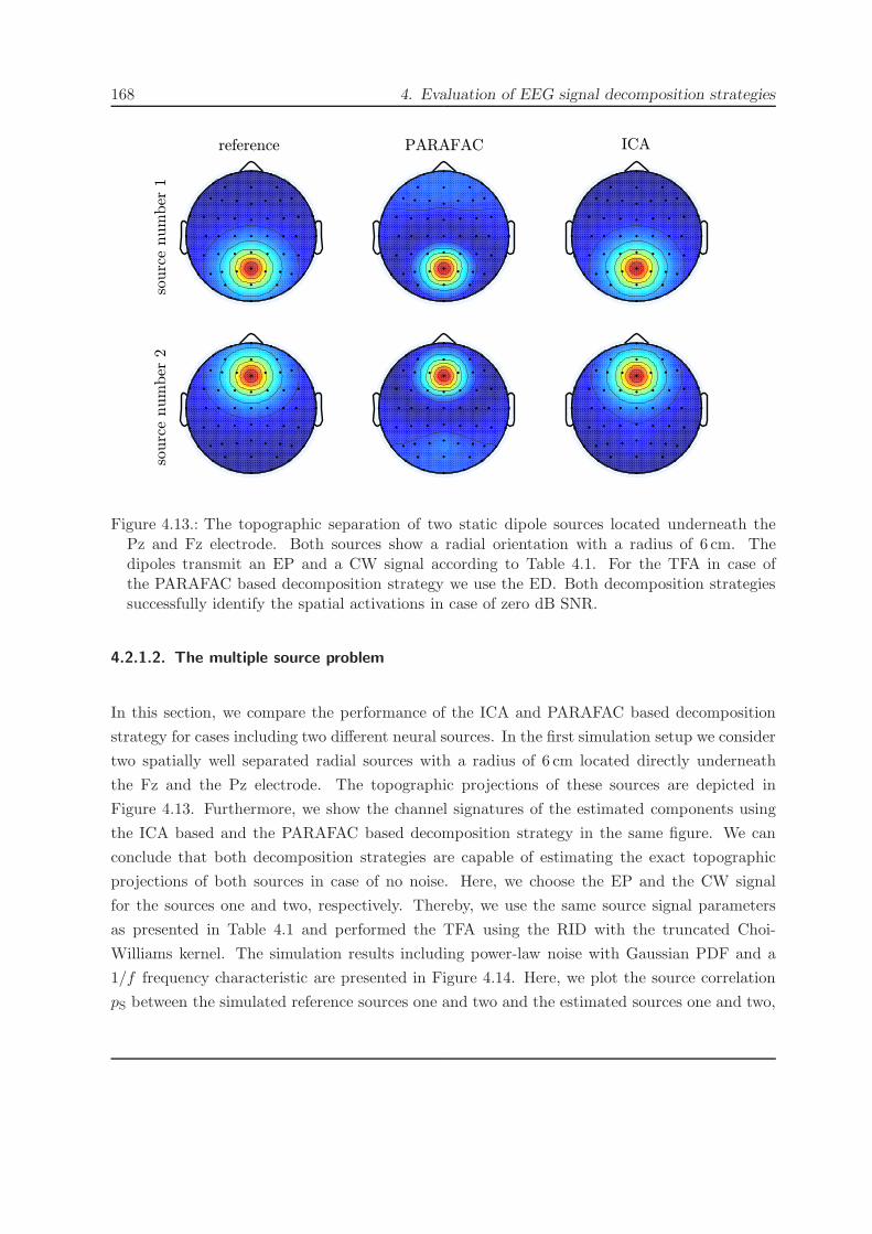
168 4. Evaluation of EEG signal decomposition strategies
!"#$%&'()*+,-./0123456789:;<=>?@ABCDEFGHIJKLMNOPQRSTUVWXYZ[\]_abcdefghijklmnopqrstuvwxyz{|}~
reference PARAFAC ICAso
urc
e num
ber
1so
urc
e num
ber
2
Figure 4.13.: The topographic separation of two static dipole sources located underneath thePz and Fz electrode. Both sources show a radial orientation with a radius of 6 cm. Thedipoles transmit an EP and a CW signal according to Table 4.1. For the TFA in case ofthe PARAFAC based decomposition strategy we use the ED. Both decomposition strategiessuccessfully identify the spatial activations in case of zero dB SNR.
4.2.1.2. The multiple source problem
In this section, we compare the performance of the ICA and PARAFAC based decomposition
strategy for cases including two different neural sources. In the first simulation setup we consider
two spatially well separated radial sources with a radius of 6 cm located directly underneath
the Fz and the Pz electrode. The topographic projections of these sources are depicted in
Figure 4.13. Furthermore, we show the channel signatures of the estimated components using
the ICA based and the PARAFAC based decomposition strategy in the same figure. We can
conclude that both decomposition strategies are capable of estimating the exact topographic
projections of both sources in case of no noise. Here, we choose the EP and the CW signal
for the sources one and two, respectively. Thereby, we use the same source signal parameters
as presented in Table 4.1 and performed the TFA using the RID with the truncated Choi-
Williams kernel. The simulation results including power-law noise with Gaussian PDF and a
1/f frequency characteristic are presented in Figure 4.14. Here, we plot the source correlation
pS between the simulated reference sources one and two and the estimated sources one and two,

4.2. Comparative performance assessment of EEG decomposition strategies based on
simulated data169
!"#$%&'()*+,-./0123456789:;<=>?@ABCDEFGHIJKLMNOPQRSTUVWXYZ[\]^_`abcdefghijklmnopqrstuvwxyz{|}~
sourc
e num
ber
1 c
orr
elation
SNR in dBSNR in dB
sourc
e num
ber
2 c
orr
elation
PARAFACJADE ICA
FastICAProKRaft ICA
PARAFACJADE ICA
FastICAProKRaft ICA
40200-20-4040200-20-40
0.1
0.2
0.3
0.4
0.5
0.6
0.7
0.8
0.9
1.0
0
0.1
0.2
0.3
0.4
0.5
0.6
0.7
0.8
0.9
1.0
0
Figure 4.14.: The source correlation (pS according to (4.14)) results for the separation of twostatic sources located at the Pz and Fz electrodes. The channel weights of these sourcesare given in Figure 4.13. Both dipoles transmitted the EP and the CW signal according toTable 4.1, respectively. For the TFA in case of the PARAFAC based decomposition strategywe use the ED.
respectively. We can conclude that the PARAFAC decomposition strategy outperforms the ICA
based decomposition strategy by approximately 10 dB at the 0.9 correlation threshold.
For the comparison of the ICA and PARAFAC based decomposition strategy over a wider range
of combinations of dipole signals and TFA methods, we again select the topography correlation
pT as a performance measure. In Figure 4.15 we present a matrix plot using four different
TFA methods and four different combinations of source signals. In all subplots we show the
topography correlation over varying SNR for both estimated sources and both decomposition
strategies. All abbreviations, source signal parameters, and TFA method parameters are the
same as in the previous Section 4.2.1.1. From these simulations, we can generally conclude that
the PARAFAC based decomposition strategy shows a superior performance over the ICA based
decomposition strategy, which is often not capable of separating both sources. This is reflected
by the fact that the ICA topography correlation does often not converge to one for high SNRs.
Additionally, we can conclude that the Wigner based TFA methods show a better performance
than the CWT. Because of the insufficient time-frequency resolution of the CWT, it is often
not possible separate the two sources. This is, e.g., the case for the EP + CW setup and the
SP + CW setup.
One very interesting question is: how far have two neural to be separated in space in order to
estimate them successfully, e.g., using the PARAFAC based decomposition strategy? A detailed

170 4. Evaluation of EEG signal decomposition strategies
!"#$%&'()*+,-./0123456789:;<=>?@ABCDEFGHIJKLMNOPQRSTUVWXYZ[\]^_`abcdefghijklmnopqrstuvwxyz{|}~
PARAFAC Source 1
SNR in dB SNR in dB SNR in dB SNR in dB
topogra
phy
corr
elation
topogra
phy
corr
elation
topog
raphy
corr
elat
ion
topog
raphy
corr
elat
ion
PARAFAC Source 2 ICA Source 1 ICA Source 2
RID PWVD SPWVD CWT
EP
+ C
WE
P +
MW
SP
+ C
WSP
+ M
W
40200-20-40 40200-20-40 40200-20-40 40200-20-400
0.5
1
0
0.5
1
0
0.5
1
0
0.5
1
Figure 4.15.: The topography correlation results for two static dipoles for varying TFA methodsand varying dipole signal combinations. The abbreviations, as well as the signal and TFA pa-rameters are given in Section 4.2.1.1. The PARAFAC and ICA based decomposition strategyare distinguished by the blue and green line colors, respectively. All solid curves are relatedto source number one and all dashed curves are related to source number two. All results areaveraged over 100 realizations.
and comprehensive answer to this question is out of the scope of this thesis, since the minimum
required distance between two sources depends on many parameters, such as the separability
of the source signals in the time-frequency domain as well as the total number sources in the
EEG. In Figure 4.16 we present an exemplary simulation with two nearby placed radial dipoles.
Thereby, the first source is located directly underneath the Pz electrode and the second source
is located midway between the Pz and CPz electrode. Both sources have a radius of 6 cm and
the dipole signals are chosen to the EP and the MW signal according to Table 4.1. For the TFA
we again use the SPWVD with the same window parameters as in Table 3.2. The simulated
reference topography of both sources is visualized on the left side of Figure 4.16. Here, we also

4.2. Comparative performance assessment of EEG decomposition strategies based on
simulated data171
!"#$%&'()*+,-./0123456789:;<=>?@ABCDEFGHIJKLMNOPQRSTUVWXYZ[\]^_`abcdefghijklmnopqrstuvwxyz{|}~
Source 1
Source 2
PARAFAC Source 1PARAFAC Source 2ICA Source 1ICA Source 2
PARAFAC Source 1PARAFAC Source 2ICA Source 1ICA Source 2
SNR in dB SNR in dB
topog
raphy c
orre
lation
topogra
phy r
econst
ruct
ion e
rror
in d
B
40200-20-400
0.1
0.2
0.3
0.4
0.5
0.6
0.7
0.8
0.9
1.0
40200-20-40-40
-35
-30
-25
-20
-15
-10
-5
0
Figure 4.16.: The topography correlation pT and topography MSE eT for two nearby placedstatic dipole sources. Both radial dipoles show a radius of 6 cm and transmit the EP and theMW signal, respectively. The first source is placed underneath the Pz electrode, while thesecond is placed midway between the Pz and CPz electrode. The signal parameters are chosenaccording to Table 4.1. For the TFA we use the SPWVD with the parameters according toSection 4.2.1.1.
present the topography correlation pT as well as the normalized topographic MSE in dB, i.e.,
10 · log10 eT. The PARAFAC based decomposition strategy is again capable to separate the two
sources, while the ICA based decomposition strategy fails to identify the first source.
Correlated sources Similar to the simulations in Section 4.2.1.1, we investigate also one two-
source scenario where the ICA assumptions of stationary and mutually independent sources
signals are violated. For this simulation we choose two radial dipoles with a radius of 6 cm each
located at the Fz and the Pz electrode. For the dipole signals we use the MW signal with the
time-varying amplitude and the EP, respectively. Thereby, the parameters of both source signals
are chosen according to Table 4.1. In order to create the additional dependency between the
power-law noise eP(t) and the source signals, we again scale the instantaneous power of the noise
with the amplitude of the MW dipole, i.e., e(t) = eP(t) ·e−(t−0.25)2
σ2 with σ = 0.05 s2. For the TFA
we use the SPWVD according to Table 3.2. In Figure 4.17 we present the topography correlation
pT as well as the topography reconstruction error in dB, i.e., 10·log10 eT for this scenario. Similar
to the single source case, we can conclude that the ICA is not capable of separating both sources.
In contrast to the ICA, the PARAFAC based decomposition strategy can be applied successfully
also in cases of non-independent and non-stationary source signals which change their amplitude
over time. Hence, these simulations confirm the theoretical advantages of the 3D PARAFAC

172 4. Evaluation of EEG signal decomposition strategies
!"#$%&'()*+,-./0123456789:;<=>?@ABCDEFGHIJKLMNOPQRSTUVWXYZ[\]^_`abcdefghijklmnopqrstuvwxyz{|}~
PARAFAC Source 1PARAFAC Source 2ICA Source 1ICA Source 2
PARAFAC Source 1PARAFAC Source 2ICA Source 1ICA Source 2
SNR in dB SNR in dB
topog
raphy c
orre
lation
topog
raphy r
econ
stru
ctio
n e
rror
in d
B
-40 -30 -20 -10 0 10 20 30 400
1.0
0.9
0.8
0.7
0.6
0.5
0.4
0.3
0.2
0.1
-30
-25
-20
-15
-10
-5
0
-40 -30 -20 -10 0 10 20 30 40
Figure 4.17.: The topography estimation results in terms of the topography correlation pT andthe topography MSE eT for two non-stationary static sources including correlated noise. Bothdipoles are placed underneath the Pz and Fz electrode and transmit the EP and MW signalaccording to Table 4.1, respectively. For the TFA we use the SPWVD with the parametersaccording to Section 4.2.1.1. All values are averaged over 100 trials.
based decomposition strategy over the 2D decomposition strategies as discussed in Section 3.3.2.
4.2.2. Assessments based on dynamic EEG sources
In the following sections, we investigate dynamic EEG sources which exhibit a virtually mov-
ing topographic activation. These types of EEG sources model the consecutive activation of
neighboring macro-columns over the cerebral cortex [173]. Thereby, the dipole signals appear
temporally shifted over the different EEG channels. This phenomenon is observed, e.g., in
the measured Visual Evoked Potentials (VEP) in Figure 3.7 and in Section 4.3. The detailed
discussion of dynamic EEG sources, as well as their simulation parameters are presented in
Section 4.1.4.2. In Section 4.2.2.1, we investigate the single dynamic source problem in order to
proof that only the PARAFAC2 decomposition strategy (cf. Section 3.3.3) is capable to model
these sources correctly. In Section 4.2.2.2, we proof that the PARAFAC2 based decomposi-
tion strategy is also capable to estimate more than one dynamic EEG source. Therefore, the
Harshman constraint (3.8), which is included in the PARAFAC2 model, is valid for many EEG
experiments. In all following simulations, we explicitly focus on the correct estimation of the
time-varying topographic projections of the dynamic EEG sources.

4.2. Comparative performance assessment of EEG decomposition strategies based on
simulated data173
!"#$%&'()*+,-./0123456789:;<=>?@ABCDEFGHIJKLMNOPQRSTUVWXYZ[\]^_`abcdefghijklmnopqrstuvwxyz{|}~
1
PARAFAC2
time in seconds
0 ms 133 ms
266 ms 400 ms
SNR in dB
sourc
e co
rrel
atio
nt0 0.40.2 -40 -20 0 20 40
0
0.1
0.2
0.3
0.4
0.5
0.6
0.7
0.8
0.9
10.03
0.025
0.02
0.015
0.01
0.005
0
-0.005
sr(t)
Figure 4.18.: Performance of the PARAFAC2 based EEG decomposition strategy in terms ofthe source correlation pS over varying SNR. The source is moving at a radius of 6 cm alongthe right temporal lobe from AF4 to POz within 400ms. The MW dipole signal is depicted inthe lower left part of the figure. In the upper left part, we visualize the time-varying spatialactivation of the source at four equidistant time snapshots.
4.2.2.1. The single source problem
In order to proof that the PARAFAC2 based decomposition strategy is able to estimate the
time-varying topography of dynamic sources, we first investigate a single radial source which
moves at a constant radius of 6 cm starting at the AF4 electrode (cf. Figure 4.3) electrode. From
this electrode, the source dipole moves in a time frame of 400ms over the right temporal lobe
towards the POz electrode. The time-varying topography of this source is depicted in the left
upper part of Figure 4.18 for four equidistant time snapshots. For the dipole signal, we choose
a Modulated Wave (MW) signal with the time-constant T = 0.005 s2 and a frequency f = 4Hz
(cf. Table 4.1). In addition to the dipole signal, we show the source correlation pS according to
equation (4.14) for the PARAFAC2 based decomposition strategy in Figure 4.18 over varying
SNR. Thereby, we consider power-law noise with a 1/f frequency characteristic and a Gaussian
PDF in order to model unspecific background EEG (cf. Section 4.1.5). For the TFA, we use
the RID with a truncated Choi-Williams kernel. We can conclude that the PARAFAC2 based
decomposition strategy shows a similar performance as the PARAFAC based decomposition
strategy applied to the single static dipole case (cf. Figure 4.10). Please note that neither
the PARAFAC based decomposition strategy nor the ICA based decomposition strategy can be
applied to dynamic sources, since they are not capable to reproduce the time-varying topography

174 4. Evaluation of EEG signal decomposition strategies
!"#$%&'()*+,-./0123456789:;<=>?@ABCDEFGHIJKLMNOPQRSTUVWXYZ[\]_abcdefghijklmnopqrstuvwxyz{|}~
PARAFAC ICA
Figure 4.19.: The topography estimations by the ICA and PARAFAC based EEG decomposi-tion strategies for the dynamic dipole source presented in Figure 4.18. Both decompositionstrategies are not capable to reconstruct the time-varying spatial activations (topography).
of such sources. In order to visualize this fact, we present the constant PARAFAC and ICA
channel weights in Figure 4.19. As we can see, both strategies approximate the time-varying
topography of the dynamic source by a constant focal topography at the time snapshot where
the dipole signal reaches its maximum amplitude (at approximately 200ms, cf. Figure 4.20).
In contrast to this, the time-varying channel signature Fr, introduced in Section 3.3.3 for the
PARAFAC2 based decomposition strategy [12], exactly describes the time-varying topography
of the dynamic source as visualized in Figure 4.20. In this figure, we present the time-varying
reference topography for the dynamic source in the top row for equidistant time snapshots. In
the second row, we present the time-varying channel signature Fr = Gr · diag(cr) estimated by
the PARAFAC2 decomposition strategy according to equation (3.9). Please note that an exact
estimation of the time-varying topography of the source is not possible at the very start (i.e.,
0ms) and at the very end (i.e., 400ms) of the time frame. This is due to the transient effects in
the TFA at these time-snapshots.
4.2.2.2. The multiple source problem
In order to show that the PARAFAC2 based decomposition strategy is also capable to extract
multiple dynamic sources albeit the implicit Harshman constraint (3.8), we choose two dynamic
radial sources with the following parameters. Both the first and second dipole source move in
a time frame of 400ms starting at the AF4 and AF3 electrode, respectively. From there, the
first source moves over the right temporal lobe towards the PO4 electrode while the second
source moves over the left temporal lobe towards the PO3 electrode. The radius of both sources
remains constant at 6 cm and the dipole direction is always radial. The resulting superimposed
topography of both sources is presented in the first row of Figure 4.21 for equidistant snapshots.

4.3. Analysis of measured EEG data 175
!"#$%&'()*+,-./0123456789:;<=>?@ABCDEFGHIJKLMNOPQRSTUVWXYZ[\]_abcdefghijklmnopqrstuvwxyz{|}~
refe
rence
PA
RA
FA
C2
50 ms 100 ms 150 ms 200 ms 250 ms 300 ms 350 ms
50 ms 100 ms 150 ms 200 ms 250 ms 300 ms 350 ms
Figure 4.20.: The estimated time-varying topography from the PARAFAC2 based decompositionstrategy for the dynamic dipole source depicted in Figure 4.18. In the upper row, we visualizethe exact topography of the source for comparison. The time-varying channel signature Fr =Gr · diag(cr) (cf. Section 3.3.3) follows exactly the topography of the simulated referencesource.
The first source sends an EP signal with f = 4Hz and T = 0.02 s2 while the second source signal
is a CW with a frequency of f = 30Hz. For the TFA, we again choose the RID with a truncated
Choi-Williams kernel. In the second and third row of Figure 4.21, we show the time-varying
channel signatures F1 and F2 extracted by the PARAFAC2 decomposition strategy. As we
can see, both estimated sources show a channel signature which follows the topography of the
corresponding original source. Therefore, we can conclude that the Harshman constraint (3.8)
(cf. Section 3.3.3) is valid for this exemplary EEG scenario, where both sources move at similar
speeds.
4.3. Analysis of measured EEG data
One of the main conclusions of the previous Section 4.2 is that the multi-dimensional EEG
decomposition strategies outperform the ICA based decomposition strategy and that only the
PARAFAC2 based decomposition strategy supports the presence of virtually moving neural
sources. Here, we prove the practicability and the advantages of the proposed PARAFAC2 based
decomposition strategy on the basis of measured Visual Evoked Potentials (VEP). Thereby,
VEP represent EEG measurements triggered to a visual stimulus such as a light flash. The
analysis of VEP is of particular interest for the test of EEG processing methods, since they are
very well investigated in literature [108, 185] and include known spatio-temporal patterns (cf.
Section 4.3.2). Furthermore, VEP are used in a variety of clinical applications [160]. In the
following, we introduce the complete signal processing chain for the decomposition of measured

176 4. Evaluation of EEG signal decomposition strategies
!"#$%&'()*+,-./0123456789:;<=>?@ABCDEFGHIJKLMNOPQRSTUVWXYZ[\]_abcdefghijklmnopqrstuvwxyz{|}~
refe
rence
sourc
e 1
sourc
e 2
50 ms 100 ms 150 ms 200 ms 250 ms 300 ms 350 ms
50 ms 100 ms 150 ms 200 ms 250 ms 300 ms 350 ms
50 ms 100 ms 150 ms 200 ms 250 ms 300 ms 350 ms
Figure 4.21.: The estimated time-varying topographies from the PARAFAC2 based decomposi-tion strategy for two dynamic dipole sources. The first source moves over the left temporallobe from AF3 to PO3, while the second source moves over the right temporal lobe from AF4to PO4. Both sources show a radial orientation over the whole time frame of 400ms and moveat a constant radius of 6 cm. The transmitted signals are the CW and the EP, respectively.The top row shows the superimposed topography of both simulated sources. The other tworows show the topographies of the two estimated PARAFAC2 components.
EEG in Section 4.3.1, before analyzing VEP using multi-dimensional decomposition strategies
in Section 4.3.2. Thereby, we show that measured VEP include visually moving neural sources
and that only the PARAFAC2 based decomposition strategy is applicable for such scenarios. As
in the previous section, we focus on the topographic analysis of the measured VEP.
4.3.1. The complete EEG signal processing chain
For the processing of measured EEG data, we have to incorporate a carefully adapted prepro-
cessing before we utilize one of the EEG decomposition strategies discussed in Section 3.3. In
Figure 4.22 we present all steps for the processing of measured EEG data using the proposed
PARAFAC2 based decomposition strategy. Here, it has to be noted that the preprocessing has
to be designed specific to certain EEG experiments, such as the measurement of Evoked Po-
tentials (EP). This preprocessing usually includes a set of linear filters, which are applied to
every EEG channel. With the help of these filters, we extract the frequency region of interest
and eliminate technical distortions such as 50Hz line noise. All linear filters have to provide a
constant group delay (i.e., a linear phase spectrum), in order to avoid phase distortions. If the

4.3. Analysis of measured EEG data 177
!"#$%&'()*+,-./0123456789:;<=>?@ABCDEFGHIJKLMNOPQRSTUVWXYZ[\]_abcdefghijklmnopqrstuvwxyz{|}~
EEG Measurements
Pre-processing
Time-Frequency Analysis
PARAFAC2 Analysis
Topographic Component
Analysis
Figure 4.22.: The complete signal processing chain for the topographic analysis of EEG. Incontrast to the PARAFAC2 based decomposition strategy in Section 3.3.3, a preprocessing isincluded for the analysis of measured EEG data. This preprocessing has to be adapted to thespecific EEG experiment.
filters are applied offline, zero phase distortion can be achieved using the forward - backward
filtering technique [89].
Very often, measured EEG data are contaminated by artifacts that share the same frequency
band with the desired EEG signals. This is especially the case for biological artifacts, such as eye
blinks, muscle artifacts or artifacts originating from the electrical activity of the heart (ECG).
In such cases the presented EEG decomposition strategies in Section 3.3 can be used in order
to separate these artifacts from the desired EEG components. In cases where the extracted
components have to be available in the time domain, also other decomposition techniques such
as the canonical correlation analysis [53,205] can be used in order to remove biological artifacts
within the preprocessing.
Since we focus on the analysis of EP, or more specific Visual Evoked Potentials (VEP), we
also incorporate an averaging technique in order to improve the SNR within the preprocessing.
This is achieved by recording multiple trials of the EP. In the sequel, these trials are averaged
synchronously to the temporal occurrence of the (visual) stimuli (stimulus triggered averaging).
This procedure is necessary, since most EP suffer from very bad SNRs.
4.3.2. Analysis of Visual Evoked Potentials (VEP)
In the following example, we analyze measured Visual Evoked Potentials (VEP) using a light
flash stimulus. The main reason for analyzing this kind of EP is that is their underlying neuro-
physiological nature leads to expected topographic patterns, which have to be extracted by the
topographic analysis. For the VEP using a light flash stimulus, we expect a strong spatial acti-
vation in the occipital region of the head directly above the visual cortex [187]. Furthermore, we
expect an subsequent activation at the motor cortex since the test person wants to close their
eye after the light-flash was presented. In the following, we describe the measurement setup

178 4. Evaluation of EEG signal decomposition strategies
as well as the preprocessing steps for the VEP data. In the sequel, we present decomposition
results using the PARAFAC2 decomposition strategy discussed in Section 3.3.3.
4.3.2.1. The measurement setup
For the visual stimulus we use a light flash which is presented to the right eye of the test person,
while the left eye is kept close using an eye-patch. Thereby, the light flash of 20ms duration
is generated by a white Light Emitting Diode (LED) located in the center of a hemispherical
perimeter. The VEP are recorded from a female test person, who is 23 years old and right-
handed. For the electrode setup we use the international 10-10 system according to Figure 4.3
measuring a total number of 64 channels using the average earlobe reference (A1 +A2)/2. The
sampling rate of the measurement system is set to 1000 sps. In order to obtain multiple trials, the
VEP experiment is repeated 1200 times. Thereby, we use randomized inter-stimulus intervals
to avoid an additional periodic excitation.
4.3.2.2. The preprocessing
For the preprocessing of the measured VEP we implement the following list of linear, time-
invariant filters:
• a 7Hz high-pass filter for the rejection of low-frequency drifts, e.g., electrode drifts;
• a 135Hz low-pass filter in order to reject high-frequency components, e.g., muscle artifacts;
• a band-stop filter in the range of 45Hz - 55Hz in order to remove 50Hz line noise.
All filters are applied offline using forward-backward filtering in order to achieve zero phase
distortions. Thereby, every filter shows a stop-band suppression of at least 60 dB. Subsequently,
we use stimulus triggered averaging over all 1200 trials in order to improve the SNR of the VEP
and to further reduce artifacts. The resulting data are depicted in the left part of Figure 4.23.
Here, we clearly observe two strong positive waves in all measured EEG channels around 100ms
and 200ms, respectively. These P100 and P200 waves are known in literature for VEP using a
light-flash stimulus [74], thus confirming the presence of VEP in these measurements. Further-
more, a temporal shift of the P100 and P200 wave is observed over the different EEG channels
(cf. the vertical black lines indicating the 100ms and 200ms time samples in Figure 4.23). This
clearly indicates the presence of dynamic EEG sources (cf. Section 4.1.4 and Section 4.2.2).

4.3. Analysis of measured EEG data 179
!"#$%&'()*+,-./0123456789:;<=>?@ABCDEFGHIJKLMNOPQRSTUVWXYZ[\]^_`abcdefghijklmnopqrstuvwxyz{|}~
-40
channel
100 200 300 400
10
20
30
40
50
60
frontal channels
time in ms
occipitalchannels
1 2 3 4 5 6 7 8 9 10
-35
-30
-25
-20
-15
-10
-5
candidate model order
norm
alize
d r
econst
ruct
ion
erro
r in
dB2
4
6
0
-2
-4
-6
P100 P200
CWTPWVDSPWVDRID
PARAFACPARAFAC2
Figure 4.23.: The modeling accuracy in terms of the rMSE eR for the PARAFAC andPARAFAC2 based decomposition strategy in case of measured VEP. The time signals ofthe VEP after the preprocessing are visualized in the left part of the figure. The right partshows the model rMSE for the TFA methods presented in Section 3.4 over a varying numberof candidate model orders R. The different parameters of the TFA methods are given inSection 4.2.1.1. Only the rMSE of the PARAFAC2 based decomposition strategy decreasessignificantly with increasing R.
4.3.2.3. Decomposition results
Before we start to discuss the topographic results of the PARAFAC2 based decomposition strat-
egy executed on the preprocessed EEG data presented in the left part of Figure 4.23, we compare
the performance of different multi-dimensional EEG decomposition strategies utilizing different
Time-Frequency Analysis (TFA) methods on the right side of Figure 4.23. Here, we present the
relative relative Mean Squared Error (rMSE) error in dB
eR = 10 · log10∥Y −Y∥2H∥Y∥2H
, (4.18)
where Y ∈ RNF×NT×NC is the measurement tensor after the TFA of the preprocessed data,
and Y is the PARAFAC / PARAFAC2 approximation of this tensor using R components.
In the right side of Figure 4.23 we depicted the rMSE over varying number of components
R. As we can see, only the PARAFAC2 decomposition leads to a clear descend in eR with
increasing number of components R. In contrast to this, the PARAFAC model shows an almost
constant rMSE as the number of components increase. This is a clear sign that the PARAFAC
model is not suited for this kind of measured VEP data. The reason for this is the presence
of dynamic EEG sources, which are only supported by the PARAFAC2 based decomposition

180 4. Evaluation of EEG signal decomposition strategies
strategy. Therefore, these results confirm the theoretic analysis in Section 3.3 and the results
based on simulated EEG in Section 4.2. Furthermore, we can conclude that the best model
accuracy is achieved using the Smoothed Pseudo Wigner-Ville Distribution (SPWVD) or the
Reduced Interference Distribution (RID) for the TFA. Thereby, both the SPWVD and the
RID provide a similar performance as already observed in Section 4.2 for the case of synthetic
EEG. Because of the slight advantages of the SPWVD over the RID in terms of cross-term
suppression (cf. Section 3.4.3), we choose the SPWVD for the following topographic analysis
using the PARAFAC2 decomposition strategy.
In Figure 4.24, we present the topographic analysis results for the measured VEP. Thereby,
the top row depicts the topographic representation of the preprocessed VEP measurements.
The time-variant topography is shown in consecutive time snapshots with a distance of 5ms
starting at 100ms. In the second and third row, we show the time-varying channel signature
Fr = Gr · diag(cr) of the PARAFAC2 decomposition strategy for r = 1 and r = 2, respectively
(cf. Section 3.3.3). With a total number of R = 2 components the PARAFAC2 model is able to
represent approximately 98% of the total power of the VEP measurements using the SPWVD
(cf. right part of Figure 4.23). We expect a strong activation at the visual cortex, as well
as an activation of the motor cortex around the C3 electrode. Especially in the region from
120ms to 150ms, component number one indicates a clear activation over the left occipital part
of the cortex directly above the left visual cortex. In the same time region we also observe a
strong activation at the C3 electrode in both components directly above the left motor cortex.
In the other time snapshots a strong activation over the left and right visual cortex is also
present. Please note that only the PARAFAC2 decomposition model enables us to identify the
different component topographies at every time instance. This is not possible using the ICA
or PARAFAC decomposition strategy, which always extract an average topographic activation
within a certain time window. Because of this, both the ICA and the PARAFAC identify only
the strongest activation over the right part of the visual cortex. Therefore, the confirmation of
the expected strong activation over the left visual cortex at 135ms to 145ms is only possible
using the proposed PARAFAC2 decomposition strategy for these VEP measurements.
Analysis of additional VEP measurements from other test persons In the following, we
analyze additional VEP measurements from three different test persons. For all test persons the
measurement setup and the preprocessing is the same as in the previous Sections 4.3.2.1 and
4.3.2.2, respectively. Thereby, every test person was measured twice under the same conditions.
For the topographic evaluation of the PARAFAC2 components, we again expect a strong spatial
activation at the occipital part of the head over the virtual cortex. Also the rMSE according

4.3. Analysis of measured EEG data 181
!"#$%&'()*+,-./0123456789:;<=>?@ABCDEFGHIJKLMNOPQRSTUVWXYZ[\]_abcdefghijklmnopqrstuvwxyz{|}~
100 ms
mea
sure
d
105 ms 110 ms 115 ms 120 ms 125 ms 130 ms 135 ms
140 ms 145 ms 150 ms 155 ms 160 ms 165 ms 170 ms 175 ms
com
p. 1
com
p. 2
mea
sure
dco
mp. 1
com
p. 2
1
-1
0
1
0
0.5
1
0
0.5
1
-1
0
1
0
0.5
1
0
0.5
Figure 4.24.: The topographic analysis of two components of neural activity extracted via thePARAFAC2 decomposition strategy in comparison to the original measured VEP (top row).Both components show the expected strong activation over the visual cortex at the back ofthe head and an activation at the motor cortex.
to equation (4.18) is analyzed for the PARAFAC and PARAFAC2 decomposition strategy with
different TFA techniques. The results of this analysis are presented in the Figures 4.25 and 4.26.
Here, we show the spatial topography of the most occipital PARAFAC2 component from every
test person. We can conclude that for every test person there is a PARAFAC2 component,
which indicates a strong activation over the virtual cortex at 120ms. Furthermore, we can
compare the topographies of the PARAFAC2 components between different VEP measurements
for the same test persons in Figures 4.25 and 4.26 at 120ms. From this comparison, we observe
that the topographies of the PARAFAC2 components of the same test persons stay similar over
different VEP measurements. This indicates that for every test person we obtain reproducible

182 4. Evaluation of EEG signal decomposition strategies
!"#$%&'()*+,-./0123456789:;<=>?@ABCDEFGHIJKLMNOPQRSTUVWXYZ[\]^_`abcdefghijklmnopqrstuvwxyz{|}~
Test Person 1
1 2 3 4 5 6 7 8 9 10-35
-30
-25
-20
-15
-10
-5
candidate model ordernor
mal
ized
rec
onst
ruct
ion
erro
r in
dB
CWTPWVDSPWVDRID
PARAFACPARAFAC2
1
0.5
0
1 2 3 4 5 6 7 8 9 10candidate model order
-35
-30
-25
-20
-15
-10
-5
nor
mal
ized
rec
onst
ruct
ion
erro
r in
dB
-40
CWTPWVDSPWVDRID
PARAFACPARAFAC2
1 2 3 4 5 6 7 8 9 10candidate model order
-35
-30
-25
-20
-15
-10
-5
nor
mal
ized
rec
onst
ruct
ion
erro
r in
dB
-40
-45
CWTPWVDSPWVDRID
PARAFACPARAFAC2
1
0.5
0
1
0.5
0
Test Person 2
Test Person 3
120 ms
120 ms
120 ms
occipital PARAFAC2 component
occipital PARAFAC2 component
occipital PARAFAC2 component
Figure 4.25.: Analysis of VEP of three test persons, first measurement.

4.3. Analysis of measured EEG data 183
!"#$%&'()*+,-./0123456789:;<=>?@ABCDEFGHIJKLMNOPQRSTUVWXYZ[\]^_`abcdefghijklmnopqrstuvwxyz{|}~
Test Person 1
1 2 3 4 5 6 7 8 9 10
-35
-30
-25
-20
-15
-10
-5
candidate model ordernor
mal
ized
rec
onst
ruct
ion
erro
r in
dB
1
0.5
0
1 2 3 4 5 6 7 8 9 10candidate model order
-30
-25
-20
-15
-10
-5
nor
mal
ized
rec
onst
ruct
ion
erro
r in
dB
1 2 3 4 5 6 7 8 9 10candidate model order
-35
-30
-25
-20
-15
-10
-5
nor
mal
ized
rec
onst
ruct
ion
erro
r in
dB
-40
-45
1
0.5
0
1
0.5
0
Test Person 2
Test Person 3
120 ms
120 ms
120 ms
occipital PARAFAC2 component
CWTPWVDSPWVDRID
PARAFACPARAFAC2
-40
CWTPWVDSPWVDRID
PARAFACPARAFAC2
occipital PARAFAC2 component
occipital PARAFAC2 component
CWTPWVDSPWVDRID
PARAFACPARAFAC2
Figure 4.26.: Analysis of VEP of three test persons, second measurement.

184 4. Evaluation of EEG signal decomposition strategies
components. From the rMSE investigations of all test persons we again can conclude that only
the PARAFAC2 based decomposition strategy is capable to model the measured VEP, i.e., the
rMSE decreases with increasing number of extracted components R. For the TFA the SPWVD
and the RID show the best performance for all test persons.
4.4. Summary
In this chapter, we analyzed the performance of the EEG decomposition strategies presented in
Chapter 3 with the help of simulated and measured EEG data. We discussed the techniques for
the generation of synthetic EEG in Section 4.1, where we used a simplified data model whose
parameters can be related to physiological features. Thereby, we made an explicit distinction
between static and dynamic EEG sources. Static sources model the spatially fixed and synchro-
nized activation of small patches in the cerebral cortex (i.e., macro-columns). In contrast to this,
dynamic sources model a consecutive activation of multiple neighboring macro-columns, which
causes a virtual movement of the source. Therefore, the topographic projection of a dynamic
source changes over time. This type of EEG source is observed, e.g., in the measured Visual
Evoked Potentials (VEP) analyzed in Section 4.3.2. The comparative performance assessment
of all EEG decomposition strategies is carried out in Section 4.2. In all simulations we chose
parameters which are typically observed in EEG measurements. This includes a realistic noise
model, which simulates the properties of unspecific background EEG. For the performance
measures used throughout these simulations, we focused primarily on the quality of the spatial
topography (also termed channel weights) of the estimated sources. In Section 4.3, we analyzed
measured EEG at the example of Visual Evoked Potentials (VEP). Thereby, we showed that
virtually moving sources occur in measured VEP and that only the PARAFAC2 based decom-
position strategy is able to analyze this kind of data. The main conclusions of the presented
simulation results are
• The three-dimensional (3D) space-time-frequency decomposition methods based on the
PARAFAC and PARAFAC2 model show a better source identification performance than
the 2D ICA based decomposition strategy. Thereby, the 3D tensor based decomposition
techniques show an improved 0.9 topography correlation threshold SNR, which is usually
4 dB to 5 dB better in comparison to the ICA based decomposition strategy.
• The ICA based decomposition strategy often fails to identify or separate sources whose
signals are non-stationary in the sense that the amplitude of the enveloping signal changes

4.4. Summary 185
over time. This is for example the case for the MW signal. The 3D tensor based decom-
position methods handle this kind non-stationary source signals successfully.
• The Continuous Wavelet Transform (CWT) does not always provide a sufficient time-
frequency resolution in order to separate typical EEG sources successfully. The time-
frequency resolution of the Wigner-based TFA methods is superior to the CWT. The Expo-
nential Distribution (ED) and the Smoothed Pseudo Wigner-Ville Distribution (SPWVD)
provide similar performance results in the synthetic EEG simulations. However, the
SPWVD is favorable because it provides the best cross-term suppression.
• The tensor based space-time-frequency decomposition methods can also be applied in cases
where the noise-parameters, such as the instantaneous noise power, are related to the time
course of the source signals. In contrast to this, the ICA based decomposition strategy
often fails in such situations. Also in cases where the source topographies are very similar
(this is the case, e.g., for nearby placed sources, cf. Figure 4.16) the 3D decomposition
techniques show a better separation performance.
• Only the PARAFAC2 based decomposition strategy is capable to identify dynamic EEG
sources. This is because both the ICA and PARAFAC based decomposition strategy are
not capable to reconstruct the time-varying topography of these sources. This major
advantage of the PARAFAC2 based decomposition strategy is also verified for the case of
measured VEP.
• The time-varying PARAFAC2 channel signatures Fr introduced in Section 3.3.3 success-
fully model the time-varying topography of dynamic EEG sources.
• Albeit the implicit Harshman constraint (3.8), the PARAFAC2 based decomposition strat-
egy is capable to separate multiple dynamic sources. This is also reflected by the fact that
the PARAFAC2 model is capable to model measured EEG in the space-time-frequency
domain with a low number of components.
The main contribution of this chapter is the systematic performance assessment and comparison
of the EEG decomposition strategies based on synthetic and measured EEG data. Furthermore,
we present a technique for the simulation of dynamic EEG sources in Section 4.1.4.2. Using
these dynamic EEG sources, we are able to verify the theoretical advantages of the PARAFAC2
based decomposition strategy introduced in Section 3.3.3. Thereby, the properties of dynamic
sources are confirmed by phenomenological observations in measured EEG (cf. Section 4.3).
The advantages of the PARAFAC2 based decomposition strategy over existing decomposition
methods is also proved on the basis of measured VEP.


187
5. Concluding remarks
Tensor decompositions which involve more than two dimensions have been applied in a variety
of applications from many scientific fields. Thereby, tensor decompositions often achieve a
superior performance compared to two-dimensional (2D) decomposition techniques, since they
are able to exploit the multi-dimensional structure of the data. Especially, the PARAllel FACtor
(PARAFAC) tensor decomposition can be applied in the context of Blind Source Separation
(BSS). In comparison to 2D BSS techniques, such as the Principal Component Analysis (PCA)
or the Independent Component Analysis (ICA), PARAFAC imposes less restrictive constraints
on the components while maintaining an unique and identifiable decomposition model. Indeed,
the only structural assumption on the PARAFAC components is that they have to be of tensor
rank-one. This is also the reason why PARAFAC has been applied for the extraction of neural
components in the ElectroEncephaloGram (EEG).
For the computation of the PARAFAC components, the normalization procedure in Section 2.3.2.4
should be applied. This normalization removes the inherent permutation and scaling ambiguity
of the PARAFAC model, which enables the exchange of different estimates of PARAFAC loading
matrices. This can be used to combine different PARAFAC model estimations in order to obtain
the best fit to the data. In the context of BSS, the PARAFAC component amplitudes can be
used in order to evaluate the influence of the different components. Also the PARAFAC2 tensor
decomposition can be normalized using the procedure in Section 2.4.2.2, which provides the same
advantages as in case of PARAFAC. For the model order estimation in case of PARAFAC2, we
recommend to use the method presented in Section 2.4.4, which is based on CORe CONsistancy
DIAgnostics (CORCONDIA).
In case of dual-symmetric and super-symmetric tensors the Procrustes estimation and Khatri-
Rao factorization (ProKRaft) algorithm for the computation of the PARAFAC model should
be applied. Thereby, ProKRaft is able to exploit the symmetric structure of the tensor in
order to reduce the amount of data to be processed. This leads to a superior performance in
comparison to other PARAFAC algorithms and provides a reduced computational complexity.
The ProKRaft algorithm can be applied to the tensor of Higher Order Cumulants (HOC) in
order to compute the ICA. The resulting ICA method shows a similar performance as current

188 5. Concluding remarks
state-of-the-art methods such as Joint Approximate Diagonalization of Eigenmatrices (JADE).
Thereby, the ProKRaft based ICA algorithm can also be applied in cases where the assumption
of statistically independent sources is not completely fulfilled. In those cases ProKRaft is able
to identify sources which are as independent as possible.
As already mentioned above, tensor decompositions such as PARAFAC or PARAFAC2 can
be utilized in order to decompose the EEG into its underlying neural components. However,
this requires the computation of at least one additional diversity (i.e., a dimension other than
space and time). Since the multi-channel EEG signals are in general non-stationary, it is pos-
sible to use a TFA in order to obtain the frequency content of the signals as a third diversity
(dimension). Thereby, only the Wigner-based TFA methods reach a superior time-frequency
resolution, which is constant over the whole frequency range. Therefore, it complies with the
demanding requirements of EEG signal analysis. For a sufficient suppression of cross-terms
either the Smoothed Pseudo Wigner-Ville Distribution (SPWVD) or a Reduced Interference
Distribution (RID), such as the Exponential Distribution (ED), have to be used. In practical
simulations based on synthetic and measured EEG, the difference between the RID and the
SPWVD is negligible. However, the SPWVD provides a more efficient cross-term suppression
with respect to the subsequent tensor decomposition, if the SPWVD parameters are chosen
appropiately.
After the TFA of the EEG signals has been performed, the EEG data are represented in the
dimensions frequency, time, and space (channels). For the subsequent three-dimensional (3D)
tensor decomposition, the use of the PARAFAC2 model constitutes many advantages over the
PARAFAC model. The resulting PARAFAC2 based EEG decomposition strategy is presented
in Section 3.3.3, and its PARAFAC2 components show a less restrictive structure than in case of
PARAFAC. This advantage is reflected by the fact that the time signatures of the PARAFAC2
components can vary over the space dimension. The resulting PARAFAC2 components are
capable to model the time-varying scalp projections of dynamic EEG sources. Furthermore, it
is possible to evaluate the exact temporal evolution of the time-varying spatial activation of such
neural sources. This is not possible when using PARAFAC.
The superior performance of multi-dimensional EEG decomposition strategies in comparison to
2D methods, such as the ICA, has been proven on the basis of synthetic EEG data. Also, the
mentioned advantages of the PARAFAC2 based decomposition strategy have been proven with
synthetic EEG simulations incorporating dynamic EEG sources. Thereby, a possible method to
simulate dynamic EEG sources with the help of moving dipoles is presented in Section 4.1.4.2.
Finally, the superior performance of the PARAFAC2 based EEG decomposition strategy is also
shown for the case of measured Visual Evoked Potentials (VEP).

189
Outlook and future work
The major advantages of the PARAFAC2 based EEG decomposition strategy over current state-
of-the-art techniques can lead to new insights for the topographical analysis of the components
of neural processing. Especially, the time-varying channel signature provides new information
which can be used, e.g., for the diagnostics of neural diseases. In order to transfer these results
to clinical applications, extensive EEG measurements of standard experiments (such as evoked
potentials), have to be performed in a clinical environment. Thereby, a sufficient amount of dif-
ferent test persons and pathological patterns have to be considered in order to obtain statistically
significant results. The processed data has to be analyzed with the help of neurologists in order
to validate the PARAFAC2 based EEG decomposition strategy based on clinical measurements.
The EEG decomposition strategies considered throughout this thesis analyze the EEG data in
the space-time-frequency domain in order to extract the scalp projections of the neural sources.
This enables a direct topographical analysis of the spatial distribution of the sources. However,
the Harshman constraint in the PARAFAC2 based decomposition strategy prohibits the analysis
of EEG data, which is generated by static and dynamic sources simultaneously. To overcome this
restriction, the incorporation of other diversities with possibly different tensor decomposition
models should be investigated. Furthermore, pre-whitening techniques, such as in [60], can be
incorporated into the decomposition strategy in order to account for colored noise. Also a direct
separation of static and dynamic neural source parameters, such as the source position and
orientation, with the help of tensor decompositions should be investigated.
For the tensor decompositions, the MOS is a crucial part in most practical applications. In case
of the PARAFAC model the MOS has been investigated extensively in [60,64,65,67]. However,
the MOS for the PARAFAC2 model is not addressed in the current state of the art. A first
method for the MOS in case of PARAFAC2 is presented in Section 2.4.4. However, other possible
methods for this problem have to be identified and investigated in detail. For EEG processing
applications, these MOS techniques have to account for colored and spatially correlated noise.
Finally, it has to be mentioned that the multi-dimensional decomposition strategies in this
thesis represent general explorative data analysis tools, which can be used in many other appli-
cations [2]. In ongoing investigations, the PARAFAC based decomposition strategy is used for
the extraction of spike features of biological neural networks. These features are used to obtain
an enhanced spike sorting algorithm which can be used to classify different cell types [5]. Also
the PARAFAC2 model can be used in order to detect and classify such neural spikes [6].


191
Appendices

193
Appendix A.
Basic tensor operations
The following notation is based on [135], except for the sub-tensors references and the ordering
of the n-mode vectors in the n-mode unfoldings (cf. Section A.3).
A.1. Higher order arrays (tensors)
A tensor of order N constitutes a multi-dimensional array of scalar values where N is the
number of dimensions. Throughout this thesis, multi-dimensional tensors (where the term multi-
dimensional is usually used if N is greater or equal than three), are denoted by capital, bold,
italic letters. Therefore, we denote an exemplary tensor of order N by
X ∈ CI1×I2×···×IN , (A.1)
where the numbers In represent the size of the tensor (i.e., a higher order array) along the n-th
dimension with n = 1, 2, . . . , N . In order to address the scalar elements of the tensor X a set of
N indices in is required such that
(X )i1,i2,...,iN = xi1,i2,...,iN with in = 1, 2, . . . , In, n = 1, 2, . . . , N . (A.2)
In Figure A.1, we show a tensor of order three with the sizes 2× 3× 2, i.e., I1 = 2, I2 = 3, and
I3 = 2. The small transparent cubes indicate the scalar values of the tensor. The direction in
which the indices in of the tensor elements change is highlighted by the arrows along the edges
of the tensor. Therefore, the tensor element with the indices i1 = 1, i2 = 1, i3 = 1 addresses
the upper left and frontal scalar value of this tensor. In some situations it is useful to address
sub-structures of a tensor X of order N . In order to do this, we use the notation
(X )in=ℓ ∈ CI1×I2···×In−1×In+1···×IN , (A.3)

194 Appendix A. Basic tensor operations
!"#$%&'()*+,-./0123456789:;<=>?@ABCDEFGHIJKLMNOPQRSTUVWXYZ[\]_abcdefghijklmnopqrstuvwxyz{|}~
i1
i2
i3
Figure A.1.: Example of a third order tensor X of size 2 × 3 × 2. Therefore, the indices in ofthe tensor elements vary in the range i1 = 1, 2; i2 = 1, 2, 3; i3 = 1, 2. The arrows indicate inwhich direction the indices in increase.
which represents a tensor of order N − 1 containing all the scalar elements of X with a fixed
index of in = ℓ. For example in Figure A.1 we can address all the elements in the frontal slice
of the tensor X (i.e., the matrix constructed from all frontal dark colored cubes) by fixing the
index i3 = 1 and therefore write (X )i3=1.
A.2. The n-mode vectors
In the same way as matrices can be handled as a set of column and row vectors, many higher
order analysis methods interpret a tensor X of order N as a collection of n-mode vectors.
The most prominent example of such a method is given by the Higher Order Singular Value
Decomposition (HOSVD) (cf. Section 2.2). Thereby, the full set of n-mode vectors of X is
obtained by varying the index in of all tensor elements within its range in = 1, 2, . . . , In while
keeping all other indices fixed. Therefore, every n-mode vector is of size In × 1 and the total
number of n-mode vectors contained in the tensor X is I1 · I2 · · · · In−1 · In+1 · · · · IN = I/In,
where I is the total number of tensor elements given by
I =N∏
n=1
In . (A.4)
All sets of n-mode vectors for an exemplary third order tensor X of size 3× 4× 3 are depicted
in Figure A.2. As we can see the sets of one-mode, two-mode and three-mode vectors are given
by all the vertical, horizontal and lateral vectors of the tensor X , respectively. Please notice

A.3. The n-mode unfoldings 195
!"#$%&'()*+,-./0123456789:;<=>?@ABCDEFGHIJKLMNOPQRSTUVWXYZ[\]_abcdefghijklmnopqrstuvwxyz{|}~
i1
i2
i3
i1
i2
i3
i1
i2
i3
a) b) c)
Figure A.2.: The n-mode vectors of third order tensor X of size 3× 4× 3. The one-mode, two-mode, and three-mode vectors are depicted in Figure a, Figure b and Figure c, respectively.They correspond to the vertical, horizontal and lateral vectors of X .
that the column vectors of a matrix alternatively could be termed the one-mode vectors, while
the row vectors of a matrix can also be referred to as the two-mode vectors.
A.3. The n-mode unfoldings
In many situations it is necessary to arrange all the elements of aN -th order tensor X in a matrix
in order to efficiently express tensor operations such as the n-mode product (cf. Appendix A.4).
One possible way to achieve this is to create matrices which collect all the n-mode vectors of the
tensor X in their columns. This procedure results in the n-mode unfoldings which are denoted
by
[X ](n) ∈ CJ×K with J = In,K = I/In . (A.5)
One degree of freedom for the generation of the n-mode unfoldings is the exact order in which
the different n-mode vectors are arranged in the columns the unfolding matrices. In [9] we in-
troduced the Matlab-like unfolding where the indices of the n-mode vectors vary in the following
ascending order
i1, i2, . . . , in−1, in+1, . . . , iN . (A.6)
This ordering of the n-mode vectors includes the advantage to be compatible to the vec(·)operator (in the sense that the indices change in the same ascending order), which leads to very
compact expressions, e.g., for the computation of the hermitian unfolding of dual-symmetric
tensors (cf. Section 2.3.3.3 equation (2.95)) and for the least squares Khatri-Rao Factorization
(cf. Appendix B.7). In fact, the vec(·) operator of a N -th order tensor can be defined using the
Matlab-like unfolding by
vec(X ) = [X ]T(N+1) . (A.7)

196 Appendix A. Basic tensor operations
Please notice that also different orderings of n-mode vectors have been defined for example
in [135]. When arranging the n-mode vectors according to (A.6) the indices j and k of the
n-mode unfolding [X ](n) are computed from the indices in of the tensor elements of X by
j = in
k = 1 +N∑
ℓ=1ℓ =n
(iℓ − 1) ·ℓ∏
q=1q =n
Iq . (A.8)
Throughout this thesis, we consistently use the Matlab-like unfolding according to (A.8). An
example of the one-mode, two-mode and three-mode unfolding of a third order tensor of size
3× 4× 3 is depicted in Figure A.3. Thereby, the order of the n-mode vectors according to (A.6)
is indicated by the different color shades.
A.4. The n-mode product
In many situations it is necessary to transform the n-mode vector space of a tensor X ∈CI1×I2···×IN of order N by multiplying all n-mode vectors from the left hand site with a matrix
A ∈ CJ×In . This operation is termed the n-mode product of the tensor X with the matrix A
and is denoted by
Y = X ×n A ∈ CI1×···×In−1×IJ×IJ+1×···×IN . (A.9)
Since all n-mode vectors of the tensor X are found in the columns of the n-mode unfolding
matrix [X ](n), their multiplication with A from the left hand site is achieved by
[Y ](n) = A · [X ](n) . (A.10)
Therefore, the n-mode product (A.9) can be implemented rearranging the n-mode unfolding
[Y ](n) according to (A.10) the resulting tensor Y . The elements of the resulting tensor Y are
therefore given by
(Y = X ×n A)i1,...,in−1,j,in+1,...,iN=
In∑
in=1
xi1,...,in−1,in,in+1,...,iN · aj,in , (A.11)
where the index j varies in the range j = 1, . . . , J . Please notice that the n-mode product
changes the size of the tensor, such that the resulting tensor Y has the size J along the n-th
dimension. Furthermore, the size rules of matrix multiplications in (A.10) have to be fulfilled,

A.4. The n-mode product 197
!"#$%&'()*+,-./0123456789:;<=>?@ABCDEFGHIJKLMNOPQRSTUVWXYZ[\]_abcdefghijklmnopqrstuvwxyz{|}~
i1i2
i3
i3
i2 i2 i2
i 1
i1i2
i3
i3
i1 i1 i1i 2
i1i2
i3
i1
i2 i2 i2 i2
i 3
Figure A.3.: The n-mode unfoldings of a third order tensor X of size 3× 4× 3. The Figures a,b and c show the one-mode, two-mode and three-mode unfoldings of X , respectively. Theindices of the n-mode vectors in the n-mode unfoldings change in ascending order.
i.e., the number of columns in the matrix A has to be equal to the size In of X along n-th
dimension. In the case of order two matrices, the one-mode product Y = X ×1 A of a matrix
X with a matrix A corresponds to the matrix multiplication from the left hand site Y = A ·Xwhile the two-mode product Y = X ×2 A corresponds the multiplication from the right hand
site Y = X ·AT. In Figure A.4, we visualize the one-mode product for an exemplary tensor X
of size 3× 4× 3 with a matrix A of size 4× 3 according to (A.10), which results in a tensor of
size 4× 4× 3.

198 Appendix A. Basic tensor operations
!"#$%&'()*+,-./0123456789:;<=>?@ABCDEFGHIJKLMNOPQRSTUVWXYZ[\]^_`abcdefghijklmnopqrstuvwxyz{|}~
=
=
i1i2
i3i1
i2
i3
[Y ](1) A [X ](1)
ji1
Figure A.4.: The one-mode product of a third order tensor X of size 3× 4× 3 with a matrix A
of size 4× 3. All one-mode vectors of the tensor X are multiplied from the left hand side byA. The size of the resulting tensor Y changes to 4× 4× 3.
A.5. The inner product and the higher order norm
The inner product between two tensors X and Y of same sizes along every dimension is denoted
by ⟨X ,Y⟩ and implemented with [135]
⟨X ,Y⟩ = vec(X )T · vec(Y) . (A.12)
With the help of this inner product definition, we can also define the higher order norm of a
tensor X as a direct generalization of the Frobenius norm of matrices by
∥X ∥H =√⟨X ,X ⟩ =
√vec(X )T · vec(X ) . (A.13)
A.6. The tensor outer product
The outer product, sometimes referred to as the tensor product, is similar to the Kronecker
matrix product (cf. Appendix B.2) in the sense that it creates all possible product pairs between
the elements of a tensor X and a tensor Y . However, the result of the outer product is a tensor.
Let us consider two tensors X ∈ CI1×I2×···×IN and Y ∈ CJ1×J2×···×JN of order N and M ,
respectively. Then, the outer product between X and Y , denoted by X ◦Y, is a tensor of order
N +M whose elements are given by
(X ◦Y)i1,i2,...,iN ,j1,j2,...,jM= xi1,i2,...,iN · yj1,j2,...,jM . (A.14)

A.7. Matrix representation of tensor equations 199
Please notice that the outer product between two vectors x and y results in a matrix which is
given by x ◦ y = x · yT. Finally, the tensor outer product is related to the Kronecker product
by
vec (X ◦Y) = vec (Y)⊗ vec (X ) . (A.15)
A.7. Matrix representation of tensor equations
The general structure of n-mode vector space transformations for a tensor X ∈ CI1×I2×···×IN
along every dimension n = 1, . . . , N using the n-mode product is given by
Y = X ×1 A(1) ×2 A
(2) ×3 · · · ×N A(N) ∈ CJ1×J2×···×JN , (A.16)
where the matrices A(n) are of size Jn × In, where Jn and In represent the sizes of the tensors
Y and X along the n-th dimension, respectively. Utilizing the Kronecker matrix product (cf.
Appendix B.2), the equation (A.16) is equivalent to the matrix expression [135]
[Y ](n) = A(n) · [X ](n) ·(A(N) ⊗A(N−1) ⊗ · · ·⊗A(n+1) ⊗A(n−1) ⊗ · · ·⊗A(1)
)T. (A.17)
Please notice that in contrast to [135] this equation includes a different order of the A(n) factors
in the Kronecker product, since we use the Matlab-like unfolding [9] according to equation (A.8).
For the second order (matrix) case a corollary of (A.17) is the following equivalence
Y = A ·X ·BT ⇐⇒ Y = X ×1 A×2 B . (A.18)
Furthermore, for the third order case we can conclude the equivalences
Y = X ×1 A×2 B ×3 C ⇐⇒
⎧⎪⎨
⎪⎩
[Y ](1) = A · [X ](1) · (C ⊗B)T
[Y ](2) = B · [X ](2) · (C ⊗A)T
[Y ](3) = C · [X ](3) · (B ⊗A)T .
(A.19)
If the tensor X is equal to the identity tensor IN,R of order N and size R along each dimension
(as it is the case in the PARAFAC model (2.44)), then the property [60]
(A(1) ⊗A(2) ⊗ · · ·⊗A(N−1)
)· [IN,R]
T(n) =
(A(1) ⋄A(2) ⋄ · · · ⋄A(N−1)
), (A.20)

200 Appendix A. Basic tensor operations
applies to equation (A.17) such that we obtain the simplified equivalence
Y = IN,R ×1 A(1) ×2 A
(2) ×3 · · ·×N A(N)
⇐⇒
[Y ](n) = A(n) ·(A(N) ⋄A(N−1) ⋄ · · · ⋄A(n+1) ⋄A(n−1) ⋄ · · · ⋄A(1)
)T.
(A.21)
A.8. Selected properties of tensor operations
The following list includes the properties of tensor operations discussed throughout this appendix
and contains some useful additional properties.
(X ×n A)×m B = (X ×n B)×m A iff n = m (A.22)
(X ×n A)×n B = X ×n (B ·A) (A.23)
(X ◦Y) ◦Z = X ◦ (Y ◦Z) (A.24)
X ◦ (Y +Z) = X ◦Y +X ◦Z (A.25)
vec(X ) = [X ]T(N+1) (A.26)
⟨X ,Y⟩ = vec(X )T · vec(Y) (A.27)
∥X ∥H =√⟨X ,X ⟩ (A.28)
vec (X ◦Y) = vec (Y)⊗ vec (X ) (A.29)(A(1) ⊗ · · · ⊗A(N−1)
)· [IN,R]
T(n) =
(A(1) ⋄ · · · ⋄A(N−1)
)(A.30)

201
Appendix B.
Selected matrix properties
B.1. The vec-permutation matrices
The vec-permutation matrix PI,J is defined by the equation
vec(A) = PI,J · vec(AT) , (B.1)
where the matrix A is of size I × J . Since both vectors vec(A) and vec(AT) contain the same
scalar elements in different order, the permutation matrix just changes the order of the elements
in vec(AT). Because of this, all rows and columns of PI,J contain only one non-zero element
with the value one. As an example, the permutation matrix P2,3 is given by
P2,3 =
⎡
⎢⎢⎢⎢⎢⎢⎢⎢⎢⎣
1 0 0 0 0 0
0 0 0 1 0 0
0 1 0 0 0 0
0 0 0 0 1 0
0 0 1 0 0 0
0 0 0 0 0 1
⎤
⎥⎥⎥⎥⎥⎥⎥⎥⎥⎦
. (B.2)
In general PI,J is of size IJ × IJ . One possible explicit definition of the permutation matrix
PI,J is given by [86]
PI,J =I∑
i=1
(eTi ⊗ IJ ⊗ ei
), (B.3)
where ei is the i-th pinning vector of size I × 1 given by the i-th column of an identity matrix
of size I × I, and IJ is the identity matrix of size J × J . The permutation matrix according
to (B.3) can also be used to change the order of factors in the Kronecker product according to
B ⊗A = PI,P · (A⊗B) · PQ,J , (B.4)

202 Appendix B. Selected matrix properties
where the matrices A and B are of size I × J and P × Q, respectively. Permutation matrices
obey some very interesting properties, such as orthogonality (i.e., PI,J · PTI,J = IIJ) and many
others. For an exhaustive discussion of these properties the reader is referred to [86].
B.2. The Kronecker matrix product
The Kronecker matrix product is of major importance for the tensor algebra, since it enables
equivalent matrix based representations of tensor equations (cf. Appendix A.7). Assuming the
matrices A ∈ CI×J and B ∈ CP×Q the Kronecker product is denoted by
C = A⊗B ∈ CIP×JQ . (B.5)
Thereby, the resulting matrix C has a block-structure where the total number of blocks is given
by the number of scalar elements in A (i.e. I ·J) and each block is of the same size as B. Every
block in the Kronecker product result C is given by
C =
⎡
⎢⎢⎢⎢⎣
a1,1 ·B a1,2 ·B · · · a1,J ·Ba2,1 ·B a2,2 ·B · · · a2,J ·B
......
. . ....
aI,1 ·B aI,2 ·B · · · aI,J ·B
⎤
⎥⎥⎥⎥⎦, (B.6)
with ai,j = (A)i,j representing the scalar elements of the matrix A. As it is easily recognized, the
Kronecker product produces a matrix containing all possible product pairs between the elements
in the matrices A and B.
B.3. The Khatri-Rao matrix product
The Khatri-Rao product is used for the matrix representation of PARAFAC tensor equations
(cf. Appendix A.7). Assuming two matrices A ∈ CI×J and B ∈ CP×J with the same number
of columns J , the Khatri-Rao product is denoted by
C = A ⋄B ∈ CIP×J . (B.7)

B.4. The Hadamard-Schur matrix product 203
Thereby, every column cj of the resulting matrix C has the structure
cj =
⎡
⎢⎢⎢⎢⎣
a1,j · bja2,j · bj
...
aI,j · bj
⎤
⎥⎥⎥⎥⎦, (B.8)
where ai,j = (A)i,j are the scalar elements of the matrix A and bj are the columns of the matrix
B for j = 1, . . . , J . As we can see, the columns of the Khatri-Rao product result C have a
Kronecker structure, i.e. the Khatri-Rao product can be seen as the column-wise Kronecker
product. Therefore, the Khatri-Rao product can also be defined as
C = [c1, c2, . . . , cJ ] = [a1 ⊗ b1,a2 ⊗ b2, . . . ,aJ ⊗ bJ ] . (B.9)
B.4. The Hadamard-Schur matrix product
The Hadamard-Schur product represents the element-wise product between two matrices A and
B of the same size I × J . It is denoted by
C = A⊙B ∈ CI×J , (B.10)
where the resulting matrix C is given by
C =
⎡
⎢⎢⎢⎢⎣
a1,1 · b1,1 a1,2 · b1,2 · · · a1,J · b1,Ja2,1 · b2,1 a2,2 · b2,2 · · · a2,J · b2,J
......
. . ....
aI,1 · bI,1 aI,2 · bI,2 · · · aI,J · bI,J
⎤
⎥⎥⎥⎥⎦. (B.11)
B.5. Properties of the Kronecker, Khatri-Rao and Hadamard-Schur
products
The following list contains important properties from matrix algebra including Kronecker, Khatri-
Rao and Hadamard-Schur products as well as the vec-Operator. For a more complete reference
on the subject the reader is referred to [38, 86, 155, 181]. The exact definitions of the following

204 Appendix B. Selected matrix properties
matrices are found in the previous sections of this appendix.
(A⊗B)⊗C = A⊗ (B ⊗C) (B.12)
A⊗ (B +C) = A⊗B +A⊗C (B.13)
(A ⋄B) ⋄C = A ⋄ (B ⋄C) (B.14)
(A⊗B)T = AT ⊗BT (B.15)
(A⊗B) · (C ⊗D) = (A ·C) ⊗ (B ·D) (B.16)
(A ⋄B)T · (A ⋄B) = (AT ·A)⊙ (BT ·B) (B.17)
A ⋄ (B +C) = A ⋄B +A ⋄C (B.18)
A⊙B = B ⊙A (B.19)
(A⊙B)⊙C = A⊙ (B ⊙C) (B.20)
A⊙ (B +C) = A⊙B +A⊙C (B.21)
B ⊗A = PI,P · (A⊗B) · PQ,J (B.22)
B ⋄A = PI,P · (A ⋄B) (B.23)
A ⋄ (BT ⋄CT) = (A ⋄CT) ⋄BT (B.24)
(A⊗B) · (C ⋄D) = (A ·C) ⋄ (B ·D) (B.25)
(A ⋄B)⊙ (C ⋄D) = (A⊙C) ⋄ (B ⊙D) (B.26)
(A⊗B)+ = A+ ⊗B+ (B.27)
(A ⋄B)+ = (AHA⊙BHB)+ · (A ⋄B)H (B.28)
vec(a · bT ) = b⊗ a (B.29)
vec(A ·B ·C) = (CT ⊗A) · vec(B) (B.30)
vec(A · diag(d) ·C) = (CT ⋄A) · d (B.31)
vec(A) = PI,J · vec(AT) (B.32)
diag(d) ·A · diag(d) = A⊙ ddT (B.33)
vec(A⊗B) =
⎛
⎜⎜⎝IJ ⊗
⎡
⎢⎢⎣
II ⊗ b1...
II ⊗ bQ
⎤
⎥⎥⎦
⎞
⎟⎟⎠ · vec(A) (B.34)
=
⎡
⎢⎢⎣
IQ ⊗ a1 ⊗ IP...
IQ ⊗ aJ ⊗ IP
⎤
⎥⎥⎦ · vec(B)

B.6. The rank and the Kruskal rank of a matrix 205
B.6. The rank and the Kruskal rank of a matrix
In general, the rank of a matrix A ∈ CI×J , denoted as rank(A), is the maximum number of
linear independent column vectors of A. The rank of A is upper bounded by the size of the
matrix such that
rank(A) ≤ min(I, J) . (B.35)
One of the fundamental properties of matrices is given by the fact that the number of linear
independent columns is always equal to the number of linear independent rows, such that the
column and row rank of a matrix are the same [85,192]
rank(A) = rank(AT) . (B.36)
In contrast to this definition, the Kruskal rank of the matrix A, denoted by rankK(A), is the
largest number k such that any subset of k column vectors of A is linear independent. From
this definition it follows directly that
rank(A) ≥ rankK(A) . (B.37)
The Kruskal rank, originally introduced in [129], has a important role for the uniqueness of
PARAFAC decompositions (cf. Section 2.3.2.2, equation (2.52)). In order to illustrate the
difference between the rank and the Kruskal rank, we assume the following exemplary matrix
A = [a1,a2,a3,a1 + a2] , (B.38)
where the vectors a1,a2, and a3 are linear independent. Then the rank of the matrix A is
obviously three, i.e., rank(A) = 3. However, the Kruskal rank is only two since the subset
[a1,a2,a1+a2] does not contain linear independent vectors. Only subsets including a maximum
number of two different columns of A are always linear independent, i.e., rankK(A) = 2.
B.7. Least Squares Khatri-Rao Factorization
In this appendix, we address the problem of identifying the Khatri-Rao factors A(n) from the
Khatri-Rao product [15]
Y = A(1) ⋄A(2) ⋄ · · · ⋄A(N) , (B.39)

206 Appendix B. Selected matrix properties
for all n = 1, . . . , N , where only the matrix Y is given. This problem is also termed the Khatri-
Rao Factorization (KRF). Thereby, Y is of size I ×R and the matrices A(n) are of size In ×R.
The number I is given by
I =N∏
n=1
In . (B.40)
Since the Khatri-Rao product in equation (B.39) is the column-wise Kronecker product (cf.
Appendix B.3) we can compute the factorization on the columns of Y = [y1,y2, . . . ,yR] and
A(n) =[a(n)1 ,a(n)
2 , . . . ,a(n)R
]separately, such that
yr = a(1)r ⊗ a(2)
r ⊗ · · ·⊗ a(N)r . (B.41)
Assuming that the sizes In are known (for every n = 1, . . . , N however, if only one of the
numbers In remains unknown it can be determined using the relation (B.40)), we can divide the
r-th column vector yr into blocks yBr,q of size IN × 1 such that
yr =
⎡
⎢⎢⎢⎢⎣
yBr,1
yBr,2...
yBr,Q
⎤
⎥⎥⎥⎥⎦, (B.42)
where the number of column blocks is given by Q = I1 · I2 · · · · IN−1. The column blocks yBr,q
can be rearranged into a matrix
[Yr](1) =[yBr,1,y
Br,2, . . . ,y
Br,Q
]∈ R
IN×Q , (B.43)
which is given by the one-mode unfolding of a tensor Yr of size IN × IN−1× · · ·× I1. Because of
equation (B.41) and the relation (A.15) between the outer product and the Kronecker product,
we can write this tensor as
Yr = a(N)r ◦ a(N−1)
r ◦ · · · ◦ a(1)r . (B.44)
From this relation it becomes evident that the columns of the Khatri-Rao factors A(n) can be
estimated in joint least squares sense by computing the best rank-one approximation of the
tensors Yr for all r = 1, . . . , R. In the 2D case (i.e., N = 2) this is possible by simply computing
the SVD of the matrix Yr = a(2)r ◦ a(1)
r and applying the Eckard-Young Theorem (2.6) (cf.
Section 2.1.2). In the higher order case for N ≥ 3, it is possible to solve (B.44) by using the HOOI
Algorithm 3 where all n-ranks are chosen to be one. In this case, the HOOI algorithm reduces to
the higher order power iteration method [136] for identifying the best rank-one approximation of

B.7. Least Squares Khatri-Rao Factorization 207
Algorithm 12 Least Squares Khatri-Rao Factorization.
Require: Matrix Y = [y1,y2, . . . ,yR] ∈ CI×R and factor matrix sizes I1, I2, . . . , INEnsure: I = I1 · I2 · . . . · IN
• for r = 1, 2, . . . , R
– create block-vectors yBr,q ∈ CIN with Q = I1 · I2 · . . . · IN−1 such that yr =
⎡
⎢⎢⎢⎣
yBr,1
yBr,2...
yBr,Q
⎤
⎥⎥⎥⎦
– create the tensor Yr by applying the one-mode inverse unfolding operation to[yBr,1,y
Br,2, . . . ,y
Br,Q
]= [Yr](1) ∈ CIN×Q
– use Algorithm 1 to calculate the Higher Order Singular Value Decomposi-
tion (HOSVD) of Yr = Sr ×1 U(1)r ×2 U
(2)r ×3 · · · ×N U
(N)r with U
(n)r =[
u(n)r,1 ,u
(n)r,2 , . . . ,uU
(n)r,In
]
– for n = 1, 2, . . . , N
∗ a(n)r = N
√(S)1,1,...,1 · u
(N−n+1)r,1
end
end
• return all A(n) =[a(n)1 ,a(n)
2 , . . . ,a(n)R
]for n = 1, . . . , N
N -th order tensors. Since the HOOI algorithm is computationally very demanding, we propose
to estimate the factor columns a(n)r separately in least squares sense from equation (B.44). This
is possible by computing the HOSVD (cf. Section 2.2) of the tensor
Yr = Sr ×1 U(1)r ×2 U
(2)r ×3 · · · ×N U (N)
r , (B.45)
where Sr ∈ RIN×IN−1×···×I1 is the HOSVD core tensor and the matrices U (n)r are the matrices of
higher order singular vectors . Here, the separate least squares estimation of the factor columns
is given by
a(n)r = N
√(Sr)1,1,...,1 · u
(N−n+1)r,1 , (B.46)
where u(N−n+1)r,1 represents the first higher order singular vector along the dimension N −n+1,
which is found in the first column of the matrix U(N−n+1)r . Please notice that the estimation of
the Khatri-Rao factors according to (B.46) resolves the inherent scaling ambiguity in (B.41) by
assigning the same Frobenius norm to each of the columns a(n)r . If any a-priory knowledge about
the norm of the factors a(n)r is available, this step should be adapted accordingly. The necessary
steps for computing the Khatri-Rao factorization (B.39) are summarized in Algorithm 12.


209
Appendix C.
The eigenvalue decomposition (EVD)
This appendix includes a short discussion of the EigenValue Decomposition (EVD) for hermitian
symmetric matrices. For a detailed discussion of this subject, the reader is referred to the classic
text books [85,192].
The eigenvalues λi as well as the eigenvectors ui of a hermitian symmetric matrix A ∈ CI×I
(i.e., A = AH) are defined according to the eigenvalue equation
A · ui = λi · ui , (C.1)
for all i = 1, . . . , I. From this eigenvalue equation, it becomes immediately clear that the
eigenvectors ui have to be restricted to unit Frobenius norm in order to make the eigenvalues
λi unique. Since the eigenvalue equation (C.1) is equivalent to the expression (A− λiI)ui = 0
and the eigenvectors ui are not allowed to be the zero-vectors, the determinant of the matrix
(A− λiI) must vanish. Therefore, the eigenvalues are the roots of the characteristic I-th order
polynomial
det(A− λiI) = 0 . (C.2)
For hermitian symmetric matrices, the solutions to (C.2) are real-valued. In order to derive the
EVD from the eigenvalue equation (C.1), we consider the columns of the following matrix
[A · u1,A · u2, . . . ,A · uI ] = [λ1 · u1,λ2 · u2, . . . ,λI · uI ] . (C.3)
By defining the matrices U = [u1,u2, . . . ,uI ] and Λ = diag(λ1,λ2, . . . ,λI) this equation can be
reformulated to
A ·U = U ·Λ . (C.4)
Since all the eigenvectors in the matrix U provide a unitary basis for the column-space of the
210 Appendix C. The eigenvalue decomposition (EVD)
matrix A, it is U ·UH = I such that we can define the EVD [85,192] as
A = U ·Λ ·UH . (C.5)
The solutions of the eigenvalue problem (C.1) can be computed by searching for the roots of the
characteristic polynomial (C.2) leading to the eigenvalues λi. In the sequel, the corresponding
eigenvectors can be determined by solving the linear set of equations (A − λiI)ui = 0. How-
ever, searching for the roots of the characteristic polynomial is a numerically badly conditioned
problem, which has to be avoided especially if the order I becomes large. Therefore, numeri-
cally stable algorithms determine the eigenvectors ui directly by exploiting the structure of the
eigenvalue decomposition (C.5) with the help of iterative Jacobi or Givens rotations [177].
One very interesting property of the eigenvectors of the matrix A is that the solution of the
maximization problem
f(x) =xHAx
∥x∥2F→ max
x, (C.6)
is provided by the eigenvector x = uimax , which corresponds to the largest eigenvalue λimax . This
becomes evident by reformulating the optimization problem (C.6) to the constraint optimization
problem
f(x) = xHAx→ maxx
subject to xH · x = 1 . (C.7)
This problem is easily solved by considering the Lagrangian function of f(x), which is given by
L(x) = f(x)− λ · (xH ·x− 1). The candidate solutions of (C.7) are now given by the vectors x
for which the gradient of the Lagrangian function L(x) is equal to zero, such that
grad(L(x)) = 2Ax− λ2x = 0 , (C.8)
which corresponds to the eigenvalue equation (C.1). The fact that (C.6) can be solved using the
eigenvalue decomposition (C.5) is commonly exploited in array signal processing methods, such
as the eigenvalue beamformer, common spatial patterns or the principal component analysis.

211
Appendix D.
Joint matrix diagonalization (JMD)
The Joint Matrix Diagonalization (JMD), also termed simultaneous matrix diagonalization, is a
class of diagonalization problems which is of major importance in Blind Source Separation (BSS)
applications. One of the most prominent examples is the JADE algorithm for the computation of
the Independent Component Analysis (ICA) [44,46]. Furthermore, JMD algorithms are related
to the PARAFAC tensor decomposition (cf. Section 2.3). The different types of JMD problems
are classified in Figure D.1. In the following, we define these types of JMD problems and refer
the reader to the corresponding references in order to obtain the algorithms for the solution of
the JMD problems.
D.1. Joint diagonalization by congruence transformations
Assume a given set of square, hermitian symmetric, and invertible matrices C(k) ∈ CN×N for
k = 1, . . . ,K. Then the problem of joint diagonalization by congruence transformations has the
structure
C(k) = A ·Λ(k) ·AH , (D.1)
where the matrix A is termed the joint diagonalizer and the matrices Λ(k) are diagonal matrices.
One of the most prominent algorithms for the solution of this problem is the AC-DC algorithm
introduced in [215]. However, recently computationally more efficient algorithms have been
introduced, e.g., in [43] and especially in [88]. If the matrices C(k) ∈ CN×N are only symmetric
(i.e., C(k) = C(k)T) then we obtain the symmetric JMD problem
C(k) = A ·Λ(k) ·AT . (D.2)
which can be solved by the symmetric version of the AC-DC algorithm presented in [214]. For
the real-valued case the JMD problems (D.1) and (D.2) are of course equivalent.
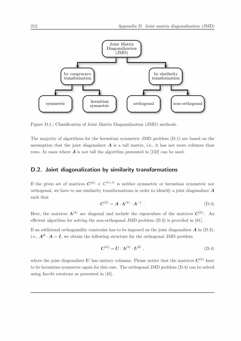
212 Appendix D. Joint matrix diagonalization (JMD)
!"#$%&'()*+,-./0123456789:;<=>?@ABCDEFGHIJKLMNOPQRSTUVWXYZ[\]_abcdefghijklmnopqrstuvwxyz{|}~
orthogonal non-orthogonalsymmetric hermitian symmetric
by congruence transformation
by similarity transformation
Joint Matrix Diagonalization
(JMD)
Figure D.1.: Classification of Joint Matrix Diagonalization (JMD) methods.
The majority of algorithms for the hermitian symmetric JMD problem (D.1) are based on the
assumption that the joint diagonalizer A is a tall matrix, i.e., it has not more columns than
rows. In cases where A is not tall the algorithm presented in [132] can be used.
D.2. Joint diagonalization by similarity transformations
If the given set of matrices C(k) ∈ CN×N is neither symmetric or hermitian symmetric nor
orthogonal, we have to use similarity transformations in order to identify a joint diagonalizer A
such that
C(k) = A ·Λ(k) ·A−1 . (D.3)
Here, the matrices Λ(k) are diagonal and include the eigenvalues of the matrices C(k). An
efficient algorithm for solving the non-orthogonal JMD problem (D.3) is provided in [81].
If an additional orthogonality constraint has to be imposed on the joint diagonalizer A in (D.3),
i.e., AH ·A = I, we obtain the following structure for the orthogonal JMD problem
C(k) = U ·Λ(k) ·UH , (D.4)
where the joint diagonalizer U has unitary columns. Please notice that the matrices C(k) have
to be hermitian symmetric again for this case. The orthogonal JMD problem (D.4) can be solved
using Jacobi rotations as presented in [45].

213
Appendix E.
The closed-form PARAFAC algorithm for symmetric
tensors
In this appendix, we derive simplified versions of the Closed-Form PARAFAC (CFP) algorithm
(cf. Section 2.3.3.2) by exploiting the additional symmetries in dual-symmetric and super-
symmetric tensors. For the sake of simplicity, we do this only for 4-th order tensors. The
generalization to tensors of order 2ND is however straight forward [162].
E.1. Dual-symmetric tensors
Assume a 4-th order dual-symmetric tensor X ∈ CI×J×I×J whose PARAFAC decomposition
according to equation (2.68) has the structure
X = I4,R ×1 A×2 B ×3 A∗ ×4 B
∗ . (E.1)
This tensor has to be permuted to XP ∈ CI×I×J×J by transposing the second and third dimen-
sion of X such that
XP = I4,R ×1 A×2 A∗ ×3 B ×4 B
∗ . (E.2)
Following the ideas presented in Section 2.3.3.2, we again exploit the connection between the
PARAFAC decomposition (E.2) and the truncated Higher Order Singular Value Decomposition
(HOSVD) of the tensor XP, which reads as
XP = S ′ ×1 U′(1) ×2 U
′(1)∗ ×3 U′(2) ×4 U
′(2)∗ . (E.3)
Here, the tensor S ′ ∈ CR×R×R×R is the truncated core tensor (2.23) and the matrices U ′(1) =
[u(1)1 ,u(1)
2 , . . . ,u(1)R ] and U ′(2) = [u(2)
1 ,u(2)2 , . . . ,u(2)
R ] contain the R dominant one-mode and
three-mode higher order singular vectors of XP, respectively (cf. Section 2.2.3.3). The number

214 Appendix E. The closed-form PARAFAC algorithm for symmetric tensors
R represents the tensor rank of X . From the matrix representation of the tensor equations (E.2)
and (E.3), which according to (A.17) reads as
[XP](1) = A · [XP](1) · (B∗ ⊗B ⊗A∗)T
= U ′(1) ·[S′]
(1)·(U ′(2)∗ ⊗U ′(2) ⊗U ′(1)∗
)T, (E.4)
we can conclude that both A and U ′(1) span the same column space, such that there exist an
invertible transformation matrix T ∈ CR×R with
A = U ′(1) · T . (E.5)
By transforming the one and two-mode vector space of XP using the basis U ′(1) we obtain
X ′P = X ×1 U
′(1) ×2 U′(1) = I4,R ×1 T ×2 T
∗ ×3 B ×4 B∗ . (E.6)
In order to transform the PARAFAC decomposition (E.6) to a hermitian symmetric Joint Matrix
Diagonalization (JMD) problem (cf. Appendix D) we stack the third order sub-tensors (X ′P)i4=ℓ
to the following third order tensor
X ′PS =
(X ′
P
)i4=183
(X ′
P
)i4=283 · · · 83
(X ′
P
)i4=I∈ C
R×R×I2 , (E.7)
where 83 denotes the concatenation of tensors along the third dimension. The PARAFAC
decomposition of the tensor X ′PS reads as
X ′PS = I3,R ×1 T ×2 T
∗ ×3 (B ⋄B∗) , (E.8)
which represents a symmetric PARAFAC according to (2.66) (cf. Section 2.3.2.5) and is therefore
equivalent to the hermitian symmetric JMD problem
(X ′
PS
)i3=ℓ
= T · diag(cℓ,:) · TH . (E.9)
for ℓ = 1, . . . , J2. Thereby, the vectors cℓ,: represent the ℓ-th row of the matrix
C = B ⋄B∗ . (E.10)

E.2. Super-symmetric tensors 215
By solving the hermitian symmetric JMD problem (E.9) using methods such as in [88], we obtain
the estimate for the PARAFAC loading matrix A by
A = U ′(1) · T . (E.11)
Furthermore, an estimate for the matrix B can be computed by the least squares Khatri-Rao
Factorization (KRF) Algorithm 12 on the matrix C according to (E.10).
Please notice that an additional estimate for both A and B can be obtained by analyzing a
second possible permutation of the original dual-symmetric tensor X , which has the PARAFAC
structure
XP2 = I4,R ×1 B ×2 B∗ ×3 A×4 A
∗ . (E.12)
The computational steps (E.3) to (E.9) have to be adapted accordingly in order process the
tensor XP2. All necessary steps for computing the dual-symmetric PARAFAC (E.13) for 4-
th order tensors, including the additional estimates obtained from XP2 , are summarized in
Algorithm 13.
E.2. Super-symmetric tensors
Assume a 4-th order super-symmetric tensor X ∈ CI×I×I×I whose PARAFAC decomposition
according to equation (2.70) has the structure
X = I4,R ×1 A×2 A×3 A×4 A . (E.13)
Following the ideas presented in Section 2.3.3.2, we again exploit the connection between the
PARAFAC decomposition (E.13) and the truncated Higher Order Singular Value Decomposition
(HOSVD) of the tensor X , which reads as
X = S ′ ×1 U′ ×2 U
′ ×3 U′ ×4 U
′ . (E.14)
Here, the tensor S ′ ∈ CR×R×R×R is the truncated core tensor (2.23) and the matrix U ′ =
[u1,u2, . . . ,uR] contains the R dominant higher order singular vectors of X (cf. Section 2.2.3.3).
The number R represents the tensor rank of X . From the matrix representation of the tensor

216 Appendix E. The closed-form PARAFAC algorithm for symmetric tensors
Algorithm 13 The closed-form PARAFAC algorithm for dual-symmetric 4-th order tensors.Require: X , tensor rank REnsure: X is dual-symmetric according to (E.1)
• determine sizes I of J along the first and second dimension of X
• create the permuted tensors XP and XP2 such that (E.2) and (E.12) hold
• compute the truncated HOSVD using Algorithm 2 of XP using inputs dn = R forn = 1, . . . , 4 obtaining U ′(1) and U ′(2)
• compute X ′P1
= XP1 ×1 U′(1) ×2 U
′(1)
• compute X ′P2
= XP2 ×1 U′(2) ×2 U
′(2)
• compute the concatenated tensor X ′PS1 =
(X ′
P1
)i4=183
(X ′
P1
)i4=283 · · · 83
(X ′
P1
)i4=I
• compute the concatenated tensor X ′PS2 =
(X ′
P2
)i4=183
(X ′
P2
)i4=283 · · · 83
(X ′
P2
)i4=J
• use the algorithm in [88] in order to jointly diagonalize the frontal slices(X ′
PS1
)i3=ℓ
for
ℓ = 1, . . . , I2 obtaining the matrices T1 and C1
• use the algorithm in [88] in order to jointly diagonalize the frontal slices(X ′
PS2
)i3=ℓ
for
ℓ = 1, . . . , J2 obtaining the matrices T2 and C2
• A = U ′(1) · T1
• B = U ′(2) · T2
• normalize the estimates A and B according to Algorithm 4
• return A, B
equations (E.13) and (E.14), which according to (A.17) reads as
[X ](1) = A · [X ](1) · (A⊗A⊗A)T
= U ′ ·[S ′]
(1)·(U ′ ⊗U ′ ⊗U ′)T , (E.15)
we can conclude that both A and U ′ span the same column space, such that there exist an
invertible transformation matrix T ∈ CR×R with
A = U ′ · T . (E.16)
By transforming the one and two-mode vector space of X using the basis U ′, we obtain
X ′ = X ×1 U′ ×2 U
′ = I4,R ×1 T ×2 T ×3 A×4 A . (E.17)
In order to transform the PARAFAC decomposition (E.17) to a symmetric Joint Matrix Diag-
onalization (JMD) problem (cf. Appendix D), we stack the third order sub-tensors (X ′)i4=ℓ to

E.2. Super-symmetric tensors 217
the following third order tensor
X ′S =
(X ′)
i4=183
(X ′)
i4=283 · · · 83
(X ′)
i4=I∈ C
R×R×I2 , (E.18)
where 83 denotes the concatenation of tensors along the third dimension. The PARAFAC
decomposition of the tensor X ′S reads as
X ′S = I3,R ×1 T ×2 T ×3 (A ⋄A) , (E.19)
which represents a symmetric PARAFAC according to (2.66) (cf. Section 2.3.2.5) and is therefore
equivalent to the symmetric JMD problem
(X ′
S
)i3=ℓ
= T · diag(cℓ,:) · TT . (E.20)
for ℓ = 1, . . . , I2. Thereby, the vectors cℓ,: represent the ℓ-th row of the matrix
C = A ⋄A . (E.21)
By solving the symmetric JMD problem (E.20) using methods such as in [214], we obtain the
estimate for the PARAFAC loading matrix A by
A = U ′ · T . (E.22)
An additional estimate for the matrix A can be obtained by computing the least squares Khatri-
Rao Factorization (KRF) Algorithm 12 on the matrixC according to (E.21). The necessary steps
for computing the super-symmetric PARAFAC (E.13) for 4-th order tensors are summarized in
Algorithm 14.

218 Appendix E. The closed-form PARAFAC algorithm for symmetric tensors
Algorithm 14 The closed-form PARAFAC algorithm for super-symmetric 4-th order tensors.Require: X , tensor rank REnsure: X is super-symmetric according to (E.13)
• determine size I of tensor X along each dimension
• compute the matrix SVD of [X ](1) = U ·Σ · V H
• construct the matrix of R dominant higher order singular vectors U ′ = [u1,u2, . . . ,uR]
• compute X ′ = X ×1 U′ ×2 U
′
• compute the concatenated tensor X ′S = (X ′)i4=1 83 (X
′)i4=2 83 · · · 83 (X′)i4=I
• use the algorithm in [88] in order to jointly diagonalize the frontal slices (X ′S)i3=ℓ for
ℓ = 1, . . . , I2 obtaining the matrices T and C
• A = U ′ · T• normalize the estimate A according to Algorithm 4
• return A

219
Appendix F.
Proofs and Derivations
In this appendix, we derive a method for solving the system of quadratic equations given by
Wk = TQkTT , (F.1)
where the known matrices Wk,Qk ∈ RRP2×RP2 are symmetric positive definite and the total
number of equations is given by I3 such that k = 1, . . . , I3. In Section F.1 we present a closed-
form solution for the unknown matrix T ∈ RRP2×RP2 , which requires at least three different
equations (F.1) in order to be unique. Since the closed-form solution for T can suffer from
numerical instabilities and is also heavily affected by noise, we introduce an iterative refinement
method in Section F.2, which uses the closed-form solution for T as an initial solution. All
computational steps for solving (F.1) are summarized in Algorithm 15.
F.1. Derivation 1
It is easily verified (by inserting equation (F.2) into (F.1) for k = ℓ1) that the solutions to an
arbitrary equation k = ℓ1 in (F.1) have the structure
T = W12ℓ1· V ·Q− 1
2ℓ1
, (F.2)
where the matrices W12ℓ1
and Q− 1
2ℓ1
have to suffice
W12ℓ1·W
T2ℓ1
= Wℓ1 (F.3)
Q− 1
2ℓ1
·Qℓ1 ·Q−T
2ℓ1
= I , (F.4)
and the matrix V ∈ RRP2×RP2 is an arbitrary unitary matrix, such that V V T = I. The
symmetric matrices W12ℓ1
and Q− 1
2ℓ1
are determined with the help of the SVD of Wℓ1 and Qℓ1 ,

220 Appendix F. Proofs and Derivations
Algorithm 15 Algorithm for the estimation of the PARAFAC2 loading matrix A under theassumption that the loading matrix C and the sample covariance H is known.Require: P, C, HEnsure: P is of size I1 × I1 × I3, C is of size I3 ×RP2, H is of size RP2 ×RP2
• compute the truncated HOSVD using Algorithm 2 of P using inputs dn = RP2 forn = 1, . . . , 3 obtaining U ′(1)
• for k = 1, 2, . . . , I3– Wk = U ′(1)T · (P)i3=k ·U ′(1)
– extract dk as the k-th row of the matrix C
– Qk = diag(dk) ·H · diag(dk)
end
• select three different numbers ℓ1, ℓ2, ℓ3 in the range of 1, . . . , I3
• compute the SVD of W− 1
2ℓ1
Wℓ2W−T
2ℓ1
= UWSWUTW
• compute the SVD of Q− 1
2ℓ1
Qℓ2Q−T
2ℓ1
= UQSQUTQ
• Q = UTQ ·Q− 1
2ℓ1
Qℓ3Q−T
2ℓ1
·UQ
• W = (W12ℓ1UW )−1 ·Wℓ3 · (W
12ℓ1UW )−T
• compute the SVD of W ⊘ Q = U SV T and extract the first singular vector u1
• T (0) = W12ℓ1·UW · diag(sgn(u1)) ·UT
Q ·Q− 12
ℓ1
• n = 0
• Repeat
– for k = 1, 2, . . . , I3
∗ e(n)k = vec
(T (n)QkT
(n)T −Wk
)
∗ F(n)k = T (n)Qk ⊗ I +
(I ⊗ T (n)Qk
)· PT
RP2,RP2
end
– F (n) =[F
(n)T
1 , . . . ,F (n)T
I3
]T
– e(n) = vec([
e(n)1 , . . . ,e(n)I3
])
– ∆T = unvec(−F (n)+ · e(n)
)
– T (n+1) = T (n) +∆T
– n = n+ 1
until convergence, i.e., ∥∆T ∥F ≈ 0
• T = T (n)
• return A = T ·U ′(1)

F.1. Derivation 1 221
respectively. The solution (F.2) determined from only one equation in (F.1) is unique up to
the unitary rotation factor V . In order to determine this rotation factor we have to insert the
solution (F.2) into a second equation k = ℓ2 in (F.1) yielding
W− 1
2ℓ1
Wℓ2W−T
2ℓ1
= V Q− 1
2ℓ1
Qℓ2Q−T
2ℓ1
V T . (F.5)
This quadratic equation has the same structure as (F.1), however the unknown matrix V is now
restricted to be unitary (unitary similarity transformation). Therefore, equation (F.5) can be
solved by computing two SVDs
W− 1
2ℓ1
Wℓ2W−T
2ℓ1
= UWSWUTW (F.6)
Q− 1
2ℓ1
Qℓ2Q−T
2ℓ1
= UQSQUTQ . (F.7)
Inserting the right sides of the SVD equations (F.6) and (F.7) into equation (F.5) yields
UW = V ·UQ , (F.8)
since SW = SQ. Therefore, the matrix V has the structure
V = UW · diag(s) ·UTQ· , (F.9)
where s is a sign vector containing entries which are either plus or minus one, i.e., s =
[±1, . . . ,±1] ∈ RRP2×1. Since the unitary rotation factor V is unique up to the unknown sign
vector s according to (F.9) we have to utilize a third equation from (F.1) in order to identify s.
Inserting the combined solution from the equations (F.2) and (F.9) given by
T = W12ℓ1·UW · diag(s) ·UT
Q ·Q− 12
ℓ1(F.10)
into the equation k = ℓ3 from (F.1) we obtain
diag(s) ·UTQ ·Q− 1
2ℓ1
Qℓ3Q−T
2ℓ1
·UQ︸ ︷︷ ︸Q
·diag(s) = (W12ℓ1UW )−1 ·Wℓ3 · (W
12ℓ1UW )−T
︸ ︷︷ ︸W
. (F.11)
This equation can be simplified using property (B.33) to
W = Q⊙ ssT . (F.12)

222 Appendix F. Proofs and Derivations
From this equation, we can determine the sign vector s by computing the SVD of the matrix
ssT = W ⊘ Q = U SV T with U = [u1, . . . , uRP2 ] , (F.13)
such that the final solution for s is given by the sign of the singular vector connected to the
largest singular value of ssT, i.e.,
s = sgn(u1) . (F.14)
F.2. Derivation 2
The closed-form solution for the system of quadratic equations (F.1) given by
T (0) = W12ℓ1·UW · diag(sgn(u1)) ·UT
Q ·Q− 12
ℓ1, (F.15)
as derived in Appendix F.1 is not always optimal. Because of additive noise as well as for
numerical reasons the residual
E(0)k = T (0)QkT
(0)T −Wk , (F.16)
does not vanish for all k = 1, . . . , I3. For this reason we derive an iterative update procedure by
computing an additive refinement ∆T on the current solution T (n) such that
T (n+1) = T (n) +∆T , (F.17)
where n is the iteration index. Thereby, we determine the additive refinement ∆T in each
iteration such that the updated residual
E(n+1)k =
(T (n) +∆T
)Qk
(T (n) +∆T
)T−Wk (F.18)
becomes as small as possible, i.e.,
min∆T∥E(n+1)
k ∥2F . (F.19)
The updated residual (F.18) can be reformulated to
E(n+1)k = T (n)QkT
(n)T +∆TQkT(n)T + T (n)Qk∆TT +∆TQk∆TT −Wk
= E(n)k +∆TQkT
(n)T + T (n)Qk∆TT +∆TQk∆TT
≈ E(n)k +∆TQkT
(n)T + T (n)Qk∆TT ,
(F.20)

F.2. Derivation 2 223
where we use the approximation ∆TQk∆TT ≈ 0 since the update ∆T is considered to be small.
In order to extract ∆T we further write
E(n+1)k = E
(n)k + I ·∆TQkT
(n)T + T (n)Qk∆TT · I , (F.21)
such that we can use the permutation matrix PTRP2,RP2
· vec(∆T (n)
)= vec
(∆T (n)T
)(cf. Ap-
pendix B.1) according to (B.3) as well property (B.30) in order to write
vec(E
(n+1)k
)= vec
(E
(n)k
)+
(T (n)Qk ⊗ I
)· vec(∆T ) +
(I ⊗ T (n)Qk
)· vec(∆TT)
= vec(E
(n)k
)+
[T (n)Qk ⊗ I +
(I ⊗ T (n)Qk
)· PT
RP2,RP2︸ ︷︷ ︸
Fk
]· vec(∆T ) . (F.22)
The reformulation of the updated residual (F.18) to the simple linear equation
vec(E
(n+1)k
)= vec
(E
(n)k
)+ Fk · vec (∆T ) (F.23)
allows us to solve the minimization problem (F.19) in least squares sense by utilizing the Moore-
Penrose pseudo-inverse with
vec (∆T ) = −F+k · vec
(E
(n)k
). (F.24)
In order to solve the minimization problem (F.19) jointly over all available equations k =
1, . . . , I3, we define the following matrices and vectors
F =
⎡
⎢⎢⎢⎢⎣
F1
F2...
FI3
⎤
⎥⎥⎥⎥⎦, e(n+1) =
⎡
⎢⎢⎢⎢⎣
vec(E(n+1)1 )
vec(E(n+1)2 )...
vec(E(n+1)I3
)
⎤
⎥⎥⎥⎥⎦, e(n) =
⎡
⎢⎢⎢⎢⎣
vec(E(n)1 )
vec(E(n)2 )
...
vec(E(n)I3
)
⎤
⎥⎥⎥⎥⎦. (F.25)
With these definitions the residual (F.23) can be computed over the full set of equations in (F.1)
by
e(n+1) = e(n) + F · vec (∆T ) , (F.26)
and therefore the joint least squares estimate for the update ∆T of the current solution T (n) is
given by
∆T = unvec(−F (n)+ · e(n)
). (F.27)

224 Appendix F. Proofs and Derivations
All computational steps which are necessary to solve system of quadratic equations (F.1) includ-
ing the closed-form initial solution derived in Appendix F.1 and the iterative refinement derived
in Appendix F.2 are summarized in Algorithm 15.
225
Appendix G.
Higher Order Moments and Cumulants
In the following, we consider a vector x of I real-valued random variables xi for i = 1, . . . , I
such that
x = [x1, x2, . . . , xI ]T . (G.1)
The definition of Higher Order Moments and Higher Order Cumulants is connected to the
characteristic function ϕ(s) of the random vector x, which is defined as [114]
ϕ(s) = E(eȷs
Tx)=
∞∫
−∞
p(x)eȷsT·xdx , (G.2)
with the vector s = [s1, s2, . . . , sI ]T and the Probability Density Function (PDF) p(x). The
connection between the PDF and the characteristic function (G.2) can be represented using the
I-dimensional inverse Fourier transform, such that
ϕ(2πs) =
∞∫
−∞
p(x)eȷ2πsT·xdx = F−1 (p(x)) . (G.3)
With the scaling property of the multi-dimensional Fourier transform, the characteristic function
is given directly as
ϕ(s) = (2π)IF−1 (p(2πx)) . (G.4)
In the following, we discuss the definitions and properties of Higher Order Moments (HOM)
and Higher Order Cumulants (HOC) as well as for the HOM tensor and the HOC tensor. The
properties of the HOM tensor and HOC tensor are also summarized in Table 2.5.

226 Appendix G. Higher Order Moments and Cumulants
G.1. Higher Order Moments
The N -dimensional Higher Order Moments (HOM) of the random vector x are defined as the
N -th order partial derivatives of the characteristic function for s = 0, such that
mom(xi1 , xi2 , . . . , xiN ) = (−ȷ)N · ∂Nϕ(s)
∂si1∂si2 · · · ∂siN
∣∣∣∣∣s=0
, (G.5)
where the indices in for n = 1, . . . , N can vary within the range 1, . . . , I. Therefore, the HOM
are the coefficients of the taylor series of the characteristic function ϕ(s) at s = 0, such that
ϕ(s) is also referred to as the moment generating function. The HOM can also be computed
from the random vector x directly using the expectation operator
mom(xi1 , xi2 , . . . , xiN ) = E (xi1 · xi2 · . . . · xiN ) . (G.6)
The HOM tensor of order N is defined as the tensor M(N)x ∈ RI×···×I which contains all N -th
order HOM of the random vector x, such that
(M
(N)x
)
i1,i2,...,iN= mom(xi1 , xi2 , . . . , xiN ) . (G.7)
Please notice that the first order HOM tensor of x is the expectation operator of x while the
second order HOM tensor of x corresponds to the correlation matrix of x. The HOM tensor
M(N)x obeys the following properties [134]
• The HOM are invariant under arbitrary index permutations. Therefore, the HOM tensor
is super-symmetric, such that(M
(N)x
)
i1,...,iN=
(M
(N)x
)
P(i1,...,iN ).
• The HOM tensor is multi-linear. Therefore, given a random vector y = A · x with a
deterministic matrix A ∈ RJ×I the HOM tensor of y is given by
M(N)y = M
(N)x ×1 A×2 · · · ×N A.
• For random variables xin with symmetric PDF the HOM of odd order N ≥ 3 vanish, i.e.,
mom (xin , . . . , xin) = 0.

G.2. Higher Order Cumulants 227
G.2. Higher Order Cumulants
The N -dimensional higher order Higher Order Cumulants (HOC) of the random vector x are
defined as the N -th order partial derivatives of ln(ϕ(s)) for s = 0, such that
cum(xi1 , xi2 , . . . , xiN ) = (−ȷ)N · ∂N ln(ϕ(s))
∂si1∂si2 · · · ∂siN
∣∣∣∣∣s=0
, (G.8)
where the indices in for n = 1, . . . , N can vary within the range 1, . . . , I. From this definition we
can conclude that the HOC represent the coefficients of the taylor series of the function ln(ϕ(s)),
which is also referred to as the cumulant generating function. The HOC are connected to the
HOM (G.6) by [134,149]
cum(xi1 , xi2 , . . . , xiN ) =∑
(−1)P−1(P−1)!·E
⎛
⎝∏
i∈S1
xi
⎞
⎠·E
⎛
⎝∏
i∈S2
xi
⎞
⎠·. . .·E
⎛
⎝∏
i∈SP
xi
⎞
⎠ , (G.9)
where the sum involves all possible partitions {S1, S2, . . . , SP } with 1 ≤ P ≤ N . For example
the first, second, third, and fourth order HOC of x are given by
cum(xi1) = E(xi1)
cum(xi1 , xi2) = E(xi1xi2)− E(xi1)E(xi2)
cum(xi1 , xi2 , xi3) = E(xi1xi2xi3)− E(xi1)E(xi2xi3)
−E(xi2)E(xi1xi3)− E(xi3)E(xi2xi1)
+2E(xi1)E(xi2)E(xi3)
cum(xi1 , xi2 , xi3 , xi4) = E{xi1xi2xi3xi4}− E{xi1}E{xi2xi3xi4}
−E{xi2}E{xi1xi3xi4}− E{xi3}E{xi1xi2xi4}
−E{xi4}E{xi1xi2xi3}− E{xi1xi2}E{xi3xi4}
−E{xi1xi3}E{xi2xi4}− E{xi1xi4}E{xi2xi3}
+2E{xi1xi2}E{xi3}E{xi4}+ 2E{xi1xi3}E{xi2}E{xi4}
+2E{xi1xi4}E{xi2}E{xi3}+ 2E{xi2xi3}E{xi1}E{xi4}
+2E{xi2xi4}E{xi1}E{xi3}+ 2E{xi3xi4}E{xi1}E{xi2}
−6E{xi1}E{xi2}E{xi3}E{xi4}

228 Appendix G. Higher Order Moments and Cumulants
The HOC tensor of order N is defined as the tensor C(N)x ∈ RI×···×I which contains all N -th
order HOC of the random vector x, such that
(C(N)x
)
i1,i2,...,iN= cum(xi1 , xi2 , . . . , xiN ) . (G.10)
Please notice that the first order HOC tensor of x is the expectation operator of x while the
second order HOC tensor of x corresponds to the covariance matrix of x. The HOC tensor C(N)x
obeys the following properties [134]
• The HOC are invariant under arbitrary index permutations. Therefore, the HOC tensor
is super-symmetric, such that(C(N)x
)
i1,...,iN=
(C(N)x
)
P(i1,...,iN ).
• The HOC tensor is multi-linear. Therefore, given a random vector y = A · x with a
deterministic matrix A ∈ RJ×I the HOC tensor of y is given by
C(N)y = C
(N)x ×1 A×2 · · ·×N A.
• For random variables xin with symmetric PDF the HOC of odd order N ≥ 3 vanish, i.e.,
cum (xin , . . . , xin) = 0.
• If two of the I random variables xin are statistically independent, the N -th order cumulant
of all variables vanishes, such that cum (xi1 , xi2 , . . . , xiN ) = 0 for N ≥ 3. If all of the
I random variables xin are mutually independent, the cumulant tensor C(N)x becomes
diagonal.
• The HOC tensor of the sum of two statistically independent random vectors x and y is
given by C(N)(y+x) = C
(N)y + C
(N)x .
• The HOC of an iid Gaussian noise vector are zero for N ≥ 3.

229
Appendix H.
The space-space-time decomposition of EEG data using
PARAFAC
The multi-dimensional decomposition strategies discussed in Section 3.3 are all based on the
analysis of time-frequency-space atoms. In order to achieve this a TFA has to be applied
to every measured EEG channel, which imposes the general assumption that the component
signals have to have a rank-one time-frequency representation. If this assumption is not valid,
the EEG decomposition strategy depicted in Figure H.1 can be applied in order to still utilize the
advantages of the multi-dimensional PARAFAC decomposition. Thereby, the resulting neural
components are represented by space-space-time atoms and no assumptions on the time course
of the component signals have to be implied. In addition, there is no assumption on the relation
between different space-space-time atoms included. However, this decomposition strategy can
only be applied for a specific spatial structure of the location of the EEG electrodes and it
imposes a constraint on the spatial distribution of the scalp projections of the neural sources.
The assumed spatial structure of the electrode placement for this decomposition strategy is
also depicted exemplary in Figure H.1 for the case of 9 measured EEG channels. In general it
must be possible to arrange all measured EEG channels in a rectangular scheme (i.e., a matrix)
without destroying the spatial relation of each electrode to its surrounding neighbors. This
is possible if a biunique left, right, upper and lower neighbor can be assigned to each EEG
electrode. As a result of the 2D rectangular representation of the electrode array we obtain two
spatial dimensions. As a consequence the EEG data can be represented by a third order tensor
X of size NC1 ×NC2 ×NT, where NC1 and NC2 represent the sizes of the 2D rectangular array
and NC1 · NC2 is the total number of measured EEG channels. Furthermore, NT represents
the number of time samples measured at each channel. Once the EEG data are represented
by the tensor X the components of neural processing are identified by applying the PARAFAC

230 Appendix H. The space-space-time decomposition of EEG data using PARAFAC
!"#$%&'()*+,-./0123456789:;<=>?@ABCDEFGHIJKLMNOPQRSTUVWXYZ[\]_abcdefghijklmnopqrstuvwxyz{|}~
chan
nel
time
chan
nel
time
chan
nel
chan
nel
time
chan
nel
chan
nel
channeltime
PARAFAC Analysis
outer-product rea-rrangement
EEG Measurements
X X
Y1
YR
Figure H.1.: The space-space-time EEG decomposition strategy based on PARAFAC. If theEEG electrodes are not already placed as a 2D rectangular array, the EEG channels X
have to be arranged in a 2D rectangular matrix while preserving the relation to neighboringchannels. As a result the EEG data can be stored in a tensor X with two spatial dimensionsand one time dimension. Subsequently, the components of neural processing are identifiedusing PARAFAC.
decomposition
X =R∑
r=1
Yr =R∑
r=1
c1,r ◦ c2,r ◦ br , (H.1)
where c1,r ∈ RNC1 and c2,r ∈ RNC2 are the channel signatures and br ∈ RNT is the time-signature
of the extracted components Yr. It has to be noted that the PARAFAC model (H.1) can also be
computed in case of missing data (missing elements in the rectangular 2D array), which provides
additional degrees of freedom for the rearrangement of the EEG electrodes to a two-dimensional
rectangular array. For more information about the computation of PARAFAC in case of missing
data the reader is referred to [194].
As already mentioned above, the decomposition strategy (H.1) provides the advantage that no
additional computational steps have to be performed in order to analyze an additional diversity
in the EEG data. Therefore, this method is computationally more efficient and there are no
assumptions on the time course and on the relation between the different component signals.
However, this EEG decomposition strategy imposes a constraint on the spatial distribution of
the scalp projections of the different EEG sources in the sense that this spatial distribution has
to be of rank-one within the 2D rectangular array. This assumption is particularly useful if the
neural sources are spatially very focused, such that only one or a small number of neighboring
electrodes is activated. For spatially largely distributed neural sources with an irregular shape

231
this decomposition strategy is less useful. In conclusion, we can state that the EEG decomposi-
tion strategy according to Figure H.1 imposes the following constraints on the structure of the
represented component signals.
• For the vast majority of the EEG electrodes it must be possible to arrange them in a 2D
rectangular scheme while preserving the relation to neighboring electrodes.
• The scalp projections of the neural sources have to be of rank-one in the arranged 2D
rectangular scheme.
• The source signals vary over the different channels only by a scalar value.


List of Figures 233
List of Figures
2.1. Visualization of the Singular Value Decomposition (SVD). . . . . . . . . . . . . . 9
2.2. Best low rank approximation of a matrix A based on the SVD. . . . . . . . . . . 11
2.3. Generalization of column and row vectors to n-mode vectors. . . . . . . . . . . . 13
2.4. The Higher Order Singular Value Decomposition of a 4× 2× 3 tensor. . . . . . . 15
2.5. The SVD as a sum of rank-one matrices. . . . . . . . . . . . . . . . . . . . . . . . 16
2.6. The PARAFAC Decomposition of a third oder tensor X of size 4 × 3 × 3 and a
tensor rank of 3. . . . . . . . . . . . . . . . . . . . . . . . . . . . . . . . . . . . . 17
2.7. The HOSVD for a third order tensor with the n-ranks R1 = 3, R2 = 2, and R3 = 2. 19
2.8. The all orthogonal slices of a third order core tensor and the corresponding one-
mode, two-mode, and three-mode singular values. . . . . . . . . . . . . . . . . . . 22
2.9. An example of a third order tensor with different n-ranks. . . . . . . . . . . . . . 23
2.10. The Tucker compression of a third order tensor utilizing the truncated HOSVD. 24
2.11. The PARAFAC representation of a third order tensor utilizing the identity tensor
and the n-mode product. . . . . . . . . . . . . . . . . . . . . . . . . . . . . . . . 31
2.12. The normalization of the third order PARAFAC decomposition using the least
squares PARAFAC amplitudes. . . . . . . . . . . . . . . . . . . . . . . . . . . . . 37
2.13. The third order symmetric PARAFAC decomposition. . . . . . . . . . . . . . . . 40
2.14. A super-symmetric third order tensor. . . . . . . . . . . . . . . . . . . . . . . . . 42
2.15. Evaluation of the MALS algorithm based on Monte-Carlo simulations. . . . . . . 47
2.16. The performance of the ProKraft algorithm based on the CCDF of the recon-
struction error. . . . . . . . . . . . . . . . . . . . . . . . . . . . . . . . . . . . . . 59
2.17. The performance of the ProKraft algorithm based on the 99-percentile of the
reconstruction error. . . . . . . . . . . . . . . . . . . . . . . . . . . . . . . . . . . 60
2.18. Comparison of different ICA algorithms . . . . . . . . . . . . . . . . . . . . . . . 66
2.19. Core consistency profile of a third order tensor . . . . . . . . . . . . . . . . . . . 68
2.20. Probability of detection over varying SNR for higher order model order selection
techniques . . . . . . . . . . . . . . . . . . . . . . . . . . . . . . . . . . . . . . . . 70
2.21. The general PARAFAC2 model . . . . . . . . . . . . . . . . . . . . . . . . . . . . 75
2.22. The PARAFAC2 model for third order tensors . . . . . . . . . . . . . . . . . . . 76

234 List of Figures
2.23. The component-wise representation of PARAFAC2 . . . . . . . . . . . . . . . . . 77
2.24. Different representations of the two-mode loading vectors in PARAFAC2 . . . . . 78
2.25. The cross-product representation of the PARAFAC2 model . . . . . . . . . . . . 79
2.26. The direct representation of the PARAFAC2 model . . . . . . . . . . . . . . . . . 82
2.27. The normalization of the PARAFAC2 model . . . . . . . . . . . . . . . . . . . . 85
2.28. Performance for the estimation of the PARAFAC2 loading matrix A. . . . . . . . 93
2.29. PARAFAC2 core consistency profile of a third order tensor . . . . . . . . . . . . 95
3.1. The structure of the cerebral cortex . . . . . . . . . . . . . . . . . . . . . . . . . 107
3.2. Radial and tangential sources in the EEG . . . . . . . . . . . . . . . . . . . . . . 109
3.3. The EEG signal decomposition strategy based on the ICA . . . . . . . . . . . . . 116
3.4. The EEG signal decomposition strategy based on the PARAFAC model. . . . . . 117
3.5. The rank-one structure of PARAFAC space-time-frequency atoms. . . . . . . . . 119
3.6. The EEG signal decomposition strategy based on the PARAFAC2 model. . . . . 120
3.7. Temporally shifted Visual Evoked Potentials (VEP) . . . . . . . . . . . . . . . . 121
3.8. Visualization of the Harshman constraint (3.8) for the PARAFAC2 model (3.7). . 122
3.9. Classification of Time-Frequency Analysis (TFA) methods considered in this thesis.124
3.10. Connections between the Wigner-Ville distribution, the temporal correlation func-
tion and the ambiguity function. . . . . . . . . . . . . . . . . . . . . . . . . . . . 129
3.11. Wigner-Ville Distribution of three modulated Gaussian impulses. . . . . . . . . . 130
3.12. The Choi-Williams and the Born-Jordan RID kernel functions. . . . . . . . . . . 132
3.13. Comparison of different TFA methods. . . . . . . . . . . . . . . . . . . . . . . . . 136
3.14. Comparison of different TFA methods. . . . . . . . . . . . . . . . . . . . . . . . . 137
3.15. The rank quality simulation results for the different TFA methods. . . . . . . . . 138
4.1. The necessary steps for the generation of synthetic EEG based on its physiological
origins. . . . . . . . . . . . . . . . . . . . . . . . . . . . . . . . . . . . . . . . . . . 145
4.2. The four layer shell model of the human head. . . . . . . . . . . . . . . . . . . . 148
4.3. The international 10-20 and 10-10 electrode setup for EEG. . . . . . . . . . . . . 150
4.4. Static and dynamic synthetic EEG sources. . . . . . . . . . . . . . . . . . . . . . 153
4.5. Example of a static radial dipole source for EEG. . . . . . . . . . . . . . . . . . . 154
4.6. Example of a dynamic radial dipole source for EEG. . . . . . . . . . . . . . . . . 157
4.7. Estimated characteristics of measured background EEG. . . . . . . . . . . . . . . 159
4.8. The topographic spatial correlation analysis for measured background EEG. . . . 160
4.9. Method for the comparison of the different EEG decomposition strategies. . . . . 161
4.10. The source correlation for one static dipole source. . . . . . . . . . . . . . . . . . 163
4.11. Topography reconstruction error and correlation for one static dipole. . . . . . . 165

List of Figures 235
4.12. The source and topography correlation for one non-stationary static source in-
cluding correlated noise. . . . . . . . . . . . . . . . . . . . . . . . . . . . . . . . . 167
4.13. The topographic separation of two static dipole sources. . . . . . . . . . . . . . . 168
4.14. Source correlation results for the separation of two static sources. . . . . . . . . . 169
4.15. The topography correlation results for two static dipoles. . . . . . . . . . . . . . 170
4.16. The topography estimation results for two nearby placed static sources. . . . . . 171
4.17. Topography estimation results for two non-stationary static sources including
correlated noise. . . . . . . . . . . . . . . . . . . . . . . . . . . . . . . . . . . . . 172
4.18. Performance of the PARAFAC2 based EEG decomposition strategy for one dy-
namic dipole source. . . . . . . . . . . . . . . . . . . . . . . . . . . . . . . . . . . 173
4.19. Topography estimations by the ICA and PARAFAC based EEG decomposition
strategies for one dynamic dipole source. . . . . . . . . . . . . . . . . . . . . . . . 174
4.20. The estimated time-varying topography from the PARAFAC2 based decomposi-
tion strategy for one dynamic dipole source. . . . . . . . . . . . . . . . . . . . . . 175
4.21. The estimated time-varying topographies from the PARAFAC2 based decompo-
sition strategy for two dynamic dipole sources. . . . . . . . . . . . . . . . . . . . 176
4.22. The complete signal processing chain for the topographic analysis of EEG. . . . . 177
4.23. Tensor decomposition accuracy for measured VEP. . . . . . . . . . . . . . . . . . 179
4.24. Topographic analysis of two components of measured VEP. . . . . . . . . . . . . 181
4.25. Analysis of measured VEP of three test persons, first measurement. . . . . . . . 182
4.26. Analysis of VEP of three test persons, second measurement. . . . . . . . . . . . . 183
A.1. Example of a third order tensor X of size 2× 3× 2. . . . . . . . . . . . . . . . . 194
A.2. The n-mode vectors of third order tensor X of size 3× 4× 3. . . . . . . . . . . . 195
A.3. The n-mode unfoldings of a third order tensor X of size 3× 4× 3. . . . . . . . . 197
A.4. The one-mode product of a third order tensor X of size 3× 4× 3 with a matrix
A of size 4× 3. . . . . . . . . . . . . . . . . . . . . . . . . . . . . . . . . . . . . . 198
D.1. Classification of Joint Matrix Diagonalization (JMD) methods. . . . . . . . . . . 212
H.1. The space-space-time EEG decomposition strategy based on PARAFAC. . . . . . 230


List of Tables 237
List of Tables
2.1. Overview of possible PARAFAC representations. . . . . . . . . . . . . . . . . . . 32
2.2. Maximum rank of third order 2-slice tensors. . . . . . . . . . . . . . . . . . . . . 34
2.3. Advantages and Disadvantages of iterative and semi-algebraic algorithms for
PARAFAC. . . . . . . . . . . . . . . . . . . . . . . . . . . . . . . . . . . . . . . . 44
2.4. Comparison in computation time for the different PARAFAC algorithms on sym-
metric tensors. . . . . . . . . . . . . . . . . . . . . . . . . . . . . . . . . . . . . . 61
2.5. Properties of the Higher Order Cumulants tensor. . . . . . . . . . . . . . . . . . . 62
2.6. Comparison between the HOSVD and PARAFAC. . . . . . . . . . . . . . . . . . 72
2.7. Overview of different PARAFAC2 representations. . . . . . . . . . . . . . . . . . 81
2.8. Comparison between PARAFAC and PARAFAC2. . . . . . . . . . . . . . . . . . 97
2.9. Overview of tensor decompositions found in literature. . . . . . . . . . . . . . . . 101
3.1. Overview of Mother Wavelets considered in this thesis. . . . . . . . . . . . . . . . 127
3.2. Simulation parameters for the investigated TFA methods. . . . . . . . . . . . . . 135
3.3. Comparison of the model assumptions inherent to the investigated EEG decom-
position strategies. . . . . . . . . . . . . . . . . . . . . . . . . . . . . . . . . . . . 140
4.1. Overview of possible dipole signals used for the generation of synthetic EEG. . . 155
4.2. The 0.9 topography correlation threshold SNR for one static dipole source. . . . 165


239
List of Algorithms
1. The algorithm for computing the HOSVD of a tensor X according to equa-
tion (2.21). Additionally, the n-mode singular values and the n-ranks are computed. 20
2. The algorithm for computing the truncated HOSVD of a tensor X of size I1 ×· · ·× IN and the n-ranks dn according to equation (2.35). . . . . . . . . . . . . . 25
3. The HOOI algorithm according to [136]. The algorithm determines the best low
n-rank approximation for given n-ranks d1, d2, . . . , dN of an N -th order tensor X
by solving (2.34) with the help of an alternating least squares algorithm. . . . . . 27
4. Normalization algorithm for the PARAFAC model utilizing the least squares
PARAFAC amplitudes according to (2.60). This normalization reduces the in-
herent PARAFAC ambiguities to a sign ambiguity. . . . . . . . . . . . . . . . . . 38
5. The multi-linear Alternating Least Squares (ALS) algorithm for the computation
of a N -th order PARAFAC decomposition of a tensor X of size I1 × · · ·× IN . It
is A(n) = [a(n)1 , . . . ,a(n)
R ]. The symbol N denotes a random variable. . . . . . . . 46
6. The Closed-Form PARAFAC (CFP) algorithm. . . . . . . . . . . . . . . . . . . 52
7. PARAllel FACtor (PARAFAC) for dual-symmetric tensors using the Procrustes
estimation and Khatri-Rao factorization (ProKRaft) algorithm. . . . . . . . . . . 57
8. The ICA algorithm based on the PARAFAC analysis of the super-symmetric
cumulant tensor using ProKRaft. The algorithm is able to run with or without
pre-whitening. . . . . . . . . . . . . . . . . . . . . . . . . . . . . . . . . . . . . . . 65
9. Normalization algorithm for the PARAFAC2 model utilizing the least squares
PARAFAC2 amplitudes according to (2.146). This normalization reduces the
inherent PARAFAC2 ambiguities to a sign ambiguity. . . . . . . . . . . . . . . . 86
10. The direct fitting algorithm [126] for the computation of the PARAFAC2 decom-
position of a third order tensor X of size I1× I2× I3. It is C = [d1,d2, . . . ,dI3 ]T.
The PARAFAC2 model order RP2 has to be known a-priori. . . . . . . . . . . . . 88
11. The algorithm for the computation of the PARAFAC2 core consistency pro-
file (2.166), which is the basis for the novel subjective PARAFAC2 CORCONDIA
for Model Order Selection. . . . . . . . . . . . . . . . . . . . . . . . . . . . . . . . 96

240 List of Algorithms
12. Least Squares Khatri-Rao Factorization. . . . . . . . . . . . . . . . . . . . . . . . 207
13. The closed-form PARAFAC algorithm for dual-symmetric 4-th order tensors. . . 216
14. The closed-form PARAFAC algorithm for super-symmetric 4-th order tensors. . . 218
15. Algorithm for the estimation of the PARAFAC2 loading matrix A under the
assumption that the loading matrix C and the sample covariance H is known. . 220

241
Glossary of Acronyms, Symbols and Notation
Acronyms
1D one-dimensional
2D two-dimensional
3D three-dimensional
AIC Akaike Information Criterium
AF Ambiguity Function
ALS Alternating Least Squares
BCI Brain Computer Interface
BEM Boundary Element Method
BSS Blind Source Separation
CANDECOMP CANonical DECOMPosition
CANDELINC CANDECOMP with LINear Constraints
CAR Common Average Reference
CCDF Complementary Cumulative Density Function
CFP Closed-Form PARAFAC
CORCONDIA CORe CONsistancy DIAgnostics
CT Computer Tomography
CW Continuous Wave
CWT Continuous Wavelet Transform
DEDICOM DEcomposition into DIrectional COMponents
DTLD Direct TriLinear Decomposition
ECG ElectroCardioGram
ED Exponential Distribution
EEG ElectroEncephaloGram
EFT Exponential Fitting Test
EMG ElectroMyoGram
EP Evoked Potentials
ERP Event Related Potentials
EVD EigenValue Decomposition
FEM Finite Element Method

242 Glossary of Acronyms, Symbols and Notation
GABA γ-aminobutyric acid
GRAM Generalized Rank Annihilation Method
HOOI Higher Order Orthogonal Iterations
HOM Higher Order Moments
HOC Higher Order Cumulants
HOSVD Higher Order Singular Value Decomposition
ICA Independent Component Analysis
INDSCAL INdividual Differences in SCALing
JADE Joint Approximate Diagonalization of Eigenmatrices
JDJT Joint Diagonalization by Jacobi Transformations
JMD Joint Matrix Diagonalization
KRF Khatri-Rao Factorization
LED Light Emitting Diode
LHS Left Hand Side
LORETA LOw Resolution Electromagnetic TomogrAphy
MDL Minimum Description Length
MEG MagnetoEncephaloGram
MIMO Multiple Input Multiple Output
MOS Model Order Selection
MRT Magnetic Resonance Tomography
MSE Mean Squared Error
MW Modulated Wave
NTF Non-negative Tensor Factorization
NP non-deterministic polynomial time
OPP Orthogonal Procrustes Problem
PARAFAC PARAllel FACtor
PARAFAC2 PARAllel FACtor2
PARALIND PARAllel profiles with LINear Dependencies
PARATUCK2 PARAFAC and TUCKer2
PCA Principal Component Analysis
PDF Probability Density Function
PSD Power Spectral Density
PWVD Pseudo Wigner-Ville Distribution
ProKRaft Procrustes estimation and Khatri-Rao factorization
RHS Right Hand Side
RID Reduced Interference Distribution
rMSE relative Mean Squared Error
SNR Signal-to-noise Ratio
SP Slow Spike
SPWVD Smoothed Pseudo Wigner-Ville Distribution

243
STD STandard deviation
STFT Short Time Fourier Transform
SVD Singular Value Decomposition
TCF Temporal Correlation Function
TFA Time-Frequency Analysis
VEP Visual Evoked Potentials
WVD Wigner-Ville Distribution
ZMCG Zero Mean Complex Gaussian
Symbols
R, R correlation matrix and tensor, respectively
C covariance matrix
E noise tensor
S core tensor of the HOSVD
M(N)x tensor of N -th order Higher Order Moments (HOM) of x
C(N)x tensor of N -th order Higher Order Cumulants (HOC) of x
U (n) Matrix of n-mode singular vectors (HOSVD)
A(n) PARAFAC n-mode loading matrix
R tensor or matrix rank
Rn multi-linear n-rank
RK Kruskal rank of a matrix
σ, Σ singular value, diagonal matrix of singular values
λ, Λ eigenvalue, diagonal matrix of eigenvalues
R set of real-valued numbers
C set of complex numbers
N set of natural numbers
N random process of Zero Mean Complex Gaussian (ZMCG) numbers
∼ distributed by
∈ included in
ȷ imaginary unit
t time
f frequency
τ delay time

244 Glossary of Acronyms, Symbols and Notation
NC number of channels
NF number of frequency samples
NT number of time samples
∞ infinity
I Identity matrix
IN,R Identity tensor of order N of size R along each dimension
Notation
a, b, c scalars
a, b, c column vectors
A, B, C matrices
X , Y , Z tensors
AT transposed of A
A+T Moore-Penrose pseudo-inverse of transposed A
(A)+∗ Moore-Penrose pseudo-inverse of the complex conjugate A
A∗ complex conjugate of A
AH Hermitian transposed of A
A−1 matrix inverse of A
A+ Moore-Penrose inverse of A
∥A∥F Frobenius norm of A
∥X ∥H higher order norm of X
⌊x⌋ round toward −∞⌈x⌉ round toward +∞{·} a set of numbers
∀ for all
E(·) expectation value
P(·) index permutation
N ! N factorial
iff if and only if
iid independent, identically distributed
s.t. such that
min(·) minimum of a function or a set of numbers
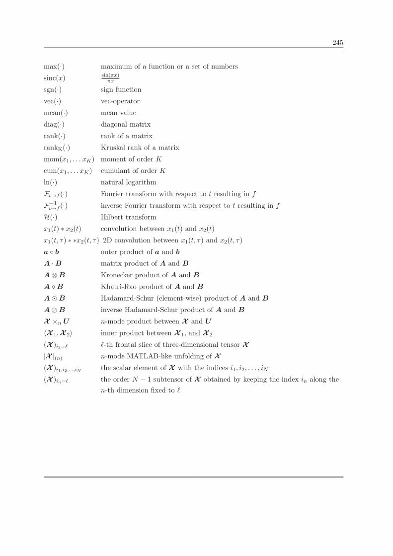
245
max(·) maximum of a function or a set of numbers
sinc(x) sin(πx)πx
sgn(·) sign function
vec(·) vec-operator
mean(·) mean value
diag(·) diagonal matrix
rank(·) rank of a matrix
rankK(·) Kruskal rank of a matrix
mom(x1, . . . xK) moment of order K
cum(x1, . . . xK) cumulant of order K
ln(·) natural logarithm
Ft→f (·) Fourier transform with respect to t resulting in f
F−1t→f (·) inverse Fourier transform with respect to t resulting in f
H(·) Hilbert transform
x1(t) ∗ x2(t) convolution between x1(t) and x2(t)
x1(t, τ) ∗ ∗x2(t, τ) 2D convolution between x1(t, τ) and x2(t, τ)
a ◦ b outer product of a and b
A ·B matrix product of A and B
A⊗B Kronecker product of A and B
A ⋄B Khatri-Rao product of A and B
A⊙B Hadamard-Schur (element-wise) product of A and B
A⊘B inverse Hadamard-Schur product of A and B
X ×n U n-mode product between X and U
⟨X 1,X 2⟩ inner product between X 1, and X 2
(X )i3=ℓ ℓ-th frontal slice of three-dimensional tensor X
[X ](n) n-mode MATLAB-like unfolding of X
(X )i1,i2,...,iN the scalar element of X with the indices i1, i2, . . . , iN
(X )in=ℓ the order N − 1 subtensor of X obtained by keeping the index in along the
n-th dimension fixed to ℓ

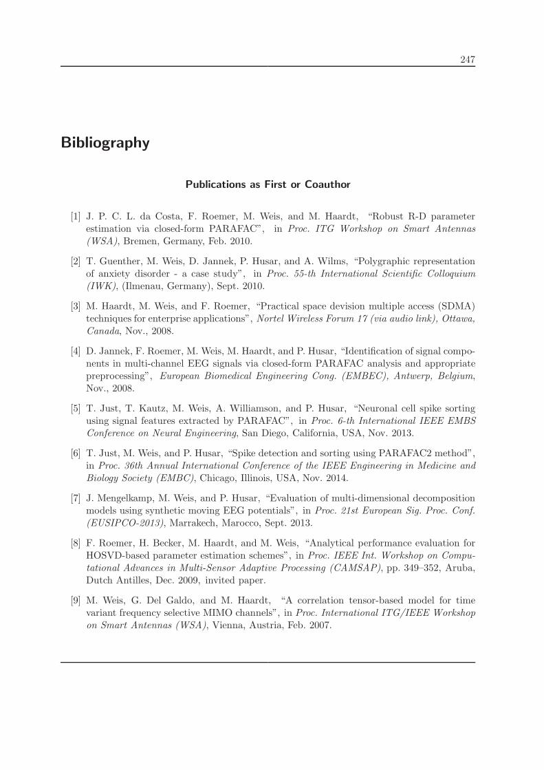
247
Bibliography
Publications as First or Coauthor
[1] J. P. C. L. da Costa, F. Roemer, M. Weis, and M. Haardt, “Robust R-D parameterestimation via closed-form PARAFAC”, in Proc. ITG Workshop on Smart Antennas(WSA), Bremen, Germany, Feb. 2010.
[2] T. Guenther, M. Weis, D. Jannek, P. Husar, and A. Wilms, “Polygraphic representationof anxiety disorder - a case study”, in Proc. 55-th International Scientific Colloquium(IWK), (Ilmenau, Germany), Sept. 2010.
[3] M. Haardt, M. Weis, and F. Roemer, “Practical space devision multiple access (SDMA)techniques for enterprise applications”, Nortel Wireless Forum 17 (via audio link), Ottawa,Canada, Nov., 2008.
[4] D. Jannek, F. Roemer, M. Weis, M. Haardt, and P. Husar, “Identification of signal compo-nents in multi-channel EEG signals via closed-form PARAFAC analysis and appropriatepreprocessing”, European Biomedical Engineering Cong. (EMBEC), Antwerp, Belgium,Nov., 2008.
[5] T. Just, T. Kautz, M. Weis, A. Williamson, and P. Husar, “Neuronal cell spike sortingusing signal features extracted by PARAFAC”, in Proc. 6-th International IEEE EMBSConference on Neural Engineering, San Diego, California, USA, Nov. 2013.
[6] T. Just, M. Weis, and P. Husar, “Spike detection and sorting using PARAFAC2 method”,in Proc. 36th Annual International Conference of the IEEE Engineering in Medicine andBiology Society (EMBC), Chicago, Illinois, USA, Nov. 2014.
[7] J. Mengelkamp, M. Weis, and P. Husar, “Evaluation of multi-dimensional decompositionmodels using synthetic moving EEG potentials”, in Proc. 21st European Sig. Proc. Conf.(EUSIPCO-2013), Marrakech, Marocco, Sept. 2013.
[8] F. Roemer, H. Becker, M. Haardt, and M. Weis, “Analytical performance evaluation forHOSVD-based parameter estimation schemes”, in Proc. IEEE Int. Workshop on Compu-tational Advances in Multi-Sensor Adaptive Processing (CAMSAP), pp. 349–352, Aruba,Dutch Antilles, Dec. 2009, invited paper.
[9] M. Weis, G. Del Galdo, and M. Haardt, “A correlation tensor-based model for timevariant frequency selective MIMO channels”, in Proc. International ITG/IEEE Workshopon Smart Antennas (WSA), Vienna, Austria, Feb. 2007.

248 Bibliography
[10] M. Weis, M. Haardt, S. Gale, and A. Jeffries, “Multi-user downlink precoding in FDDsystems without channel feedback”, in Proc. of the 20-th Meeting of the Wireless WorldResearch Forum (WWRF), Ottawa, Canada, Apr. 2008.
[11] M. Weis and P. Husar, “Joint space-time-frequency decomposition of event related EEGdata using the PARAFAC2 tensor model”, in Proc. of International Doctoral Seminar(IDS), Smolenice Castle, Slovakia, May, 2012.
[12] M. Weis, D. Jannek, T. Guenther, P. Husar, M. Haardt, and F. Roemer, “Temporallyresolved multi-way component analysis of dynamic sources in event-related EEG datausing PARAFAC2”, in Proc. 18-th European Signal Processing Conference (EUSIPCO),Aalborg, Denmark, Aug. 2010.
[13] M. Weis, D. Jannek, T. Guenther, P. Husar, M. Haardt, and F. Roemer, “Space-time-frequency component analysis of visual evoked potentials based on the PARAFAC2model”, in Proc. 55-th International Scientific Colloquium (IWK), Ilmenau, Germany,Sept. 2010.
[14] M. Weis, D. Jannek, F. Roemer, T. Guenther, M. Haardt, and P. Husar, “Multi-dimensional PARAFAC2 component analysis of multi-channel eeg data including temporaltracking”, in Proc. 32-th International Conference of the IEEE Engineering in Medicineand Biology Society (EMBC), Buenos Aires, Argentina, Sept. 2010.
[15] M. Weis, F. Roemer, M. Haardt, and P. Husar, “Dual-Symmetric parallel factor analysisusing procrustes estimation and Khatri-Rao factorization”, in Proc. 20-th European Sig.Proc. Conf. (EUSIPCO-2012), Bucharest, Romania, Aug 2012.
[16] M. Weis, F. Roemer, M. Haardt, D. Jannek, and P. Husar, “Multi-dimensional space-time-frequency component analysis of event-related EEG data using closed-form PARAFAC”,in Proc. IEEE Int. Conference on Acoustics, Speech, and Signal Processing (ICASSP), pp.349–352, Taipei, Taiwan, Apr. 2009.
References by Other Authors
[17] B. M. Abadi, D. Jarchi, and S. Sanei, “Simultaneous localization and separation of biomed-ical signals by tensor factorization”, in Proc. IEEE/SP 15th Workshop on Statistical SignalProcessing, pp. 61–78, 2009.
[18] E. Acar, C. A. Bingol, H. Bingol, R. Bro, and B. Yener, “Multiway analysis of epilepsytensors”, ISMB/ECCB, vol. 23, pp. 10–18, 1997.
[19] E. Acar, C. A. Bingol, H. Bingol, and B. Yener, “Computational analysis of epilepticfocus localization”, in In Proceedings of the Fourth IASTED International Conference onBiomedical Engineering, pp. 317–322, 2006.
[20] E. Acar, S. A. Camtepe, M. S. Krishnamoorthy, and B. Yener, “Modeling and multiwayanalysis of chatroom tensors”, ISI 2005: Proceedings of the IEEE International Conferenceon Intelligence and Security Informatics, pp. 256 —- 268, 2005.
Bibliography 249
[21] E. Acar and B. Yener, “Unsupervised multiway data analysis: A literature survey”,Knowledge and Data Engineering, IEEE Transactions on, vol. 21, no. 1, pp. 6–20, 2009.
[22] H. Akaike, “A new look at the statistical model identification”, Automatic Control, IEEETransactions on, vol. 19, no. 6, pp. 716–723, 1974.
[23] L. Albera, A. Ferreol, D. C. Rimele, I. Merlet, and F. Wendling, “Brain source localizationusing a fourth-order deflation scheme”, IEEE Transactions on Biomedical Engineering,vol. 55, pp. 490–501, Feb. 2008.
[24] C. M. Andersen and R. Bro, “Practical aspects of parafac modeling of fluorescenceexcitation-emission data”, Journal of Chemometrics, vol. 17, no. 4, pp. 200–215, 2003.
[25] C. A. Andersson and R. Bro, “The N -way toolbox for MATLAB”, Chemometrics andIntelligent Laboratory Systems, vol. 52, no. 1, pp. 1–4, 2000.
[26] C. J. Appellof and E. R. Davidson, “Strategies for analyzing data from video fluorometricmonitoring of liquid chromatographic effluents”, Analytical Chemistry, vol. 53, no. 13, pp.2053–2056, 1981.
[27] A. Araque and G. Perea, “Glial modulation of synaptic transmission in culture”, Glia,vol. 47, no. 3, pp. 241–248, 2004.
[28] B. W. Bader, M. W. Berry, and M. Browne, “Discussion tracking in enron email usingparafac. in survey of text mining: Clustering, classification, and retrieval”, M. W. Berryand M. Castellanos Eds. Springer, vol. 2nd Ed., pp. 147–162, 2007.
[29] S. Baillet, J. C. Mosher, and R. M. Leahy, “Electromagnetic brain mapping”, SignalProcessing Magazine, IEEE, vol. 18, no. 6, pp. 14–30, 2001.
[30] M. F. Bear, B. W. Conners, and M. A. Paradiso, Neuroscience: Exploring the Brain,Williams & Wilkins, 1996.
[31] H. Becker, “Tensor-based techniques for EEG source localization”, Bachelor thesis, Ilme-nau University of Technology, Sophia-Antipolis, Frankreich, Mar. 2010.
[32] H. Becker, P. Comon, L. Albera, M. Haardt, and I. Merlet, “Multiway space-time-wave-vector analysis for source localization and extraction”, in Proc. 18-th European SignalProcessing Conference (EUSIPCO), Aalborg, Denmark, Aug. 2010.
[33] E. Beltrami, “Sulle funzioni bilineari”, Giornale di Matematiche ad Uso degli StudentiDelle Universita, vol. 11, pp. 98–106, 1873, English translation by Daniel Boley availablefrom (1995).
[34] J. M. F. Berge and H. A. L. Kiers, “Some uniqueness results for PARAFAC2”, Psychome-trika, vol. 61, no. 1, pp. 123–132, 1996.
[35] J. M. F. Ten Berge, “Kruskals polynomial for 2 × 2 × 2 arrays and a generalization to2× n× n arrays”, Psychometrika, vol. 56, pp. 631–636, 1991.

250 Bibliography
[36] J. M. F. Ten Berge and N. D. Sidiropoulos, “On uniqueness in candecomp/parafac”,Psychometrika, vol. 67, no. 3, pp. 399–409, 2002.
[37] B. Boashash, Time Frequency Signal Analysis and Processing: A Comprehensive Refer-ence, Elsevier Science, 2003.
[38] J. W. Brewer, “Kronecker product and matrix calculus in system theory”, IEEE Trans-actions on Circuits and Systems, vol. CAS-25, no. 9, pp. 772–781, Sept. 1978.
[39] R. Bro, “PARAFAC. tutorial and applications”, in Chemometrics and Intelligent Labo-ratory Systems, 38, pp. 149–171, 1997.
[40] R. Bro, C. A. Andersson, and H. A. L. Kiers, “PARAFAC2 — Part II. Modeling chro-matographic data with retention time shifts”, J. Chemometrics, vol. 13, pp. 295–309,1999.
[41] R. Bro, R.A. Harshman, and N. D. Sidiropoulos, “Modeling multi-way data with linearlydependent loadings”, Technical Report 2005-176, KVL, 2005.
[42] R. Bro and H. A. L. Kiers, “A new efficient method for determining the number ofcomponents in parafac models”, Journal of Chemometrics, vol. 17, no. 5, pp. 274–286,2003.
[43] A. Bunse-Gerstner, R. Byers, and V. Mehrmann, “Numerical methods for simultaneousdiagonalization”, SIAM J. Matrix Anal. Applicat, vol. 14, pp. 927–949, 1993.
[44] J. F. Cardoso, “High-order contrasts for independent component analysis”, Neural Com-putation, vol. 11, no. 1, pp. 157–192, Jan 1999.
[45] J. F. Cardoso and A. Souloumiac, “Jacobi angels for simultaneous diagonalization”, SIAMJ. Matrix Anal. Appl., vol. 17, no. 1, pp. 161–164, 1996.
[46] J. F. Cardoso and A. Souloumiac, “Blind beamforming for non gaussian signals”, IEEEProceedings-F, vol. 140, pp. 362–370, Dec. 1993.
[47] J. D. Carroll and J. Chang, “Analysis of individual differences in multidimensional scalingvia an n-way generalization of ‘eckart-young’ decomposition”, Psychometrika, vol. 35, pp.283–319, 1970.
[48] J. D. Carroll, S. Pruzansky, and J. B. Kruskal, “Candelinc: A general approach to mul-tidimensional analysis of many-way arrays with linear constraints on parameters”, Psy-chometrika, vol. 45, no. 1, pp. 3–24, 1980.
[49] P. A. Chew, B. W. Bader, T. G. Kolda, and A. Abdelali, “Cross-language informationretrieval using parafac2”, in Proceedings of the 13th ACM SIGKDD international confer-ence on Knowledge discovery and data mining, KDD ’07, pp. 143–152, New York, NY,USA, 2007.
[50] H. Choi and W. J. Williams, “Improved time-frequency representation of multicomponentsignals using exponential kernels”, in IEEE Trans. Acoust., Speech, Signal Process., vol. 37,pp. 862–871, 1989.

Bibliography 251
[51] A. Cichocki and S. ichi Amari, Adaptive Blind Signal and Image Processing - LearningAlgorithms and Applications, Wiley, 2002.
[52] A. Cichocki, R. Zdunek, A. H. Phan, and S. Amari, Nonnegative Matrix and TensorFactorizations: Applications to Exploratory Multi-way Data Analysis and Blind SourceSeparation, Wiley, Sept. 2009.
[53] W. De Clercq, A. Vergult, B. Vanrumste, W. Van Paesschen, and S. Van Huffel, “Canonicalcorrelation analysis applied to remove muscle artifacts from the electroencephalogram”,Biomedical Engineering, IEEE Transactions on, vol. 53, no. 12, pp. 2583–2587, 2006.
[54] L. Cohen, Time-Frequency Analysis: Theory and Applications, Prentice Hall, UpperSaddle River, NJ, 1995.
[55] P. Comon, “Independent component analysis, a new concept?”, Signal Process., SpecialIssue on Higher Order Statistics, vol. 36, no. 3, pp. 287–314, 1994.
[56] P. Comon, “Tensor decompositions, State of the art and applications”, IMA Conf. math-ematics in Signal Processing, Warwick, UK, 2000.
[57] P. Comon, “Tensor diagonalization, a useful tool in signal processing”, 10th IFAC SYIDSymp., vol. 1, pp 77–88, Copenhagen, Denmark, 2001.
[58] P. Comon, B. Mourrain, L.-H. Lim, and G.H. Golub, “Genericity and rank deficiencyof higher order symmetric tensors”, 31st IEEE INT CONF. Acoust. Speech Signal Proc.(ICASSP), 2006.
[59] P. Comon, J. ten Berge, L. De Lathauwer, and J. Castaing, “Generic and typical ranksof multi-way arrays”, Linear Algebra and Its Applications, vol. 430, no. 11—12, pp. 2997–3007, 2009.
[60] J. P. C. L. Da Costa, Parameter Estimation Techniques for Multi-Dimensional ArraySignal Processing, PhD thesis, Ilmenau University of Technology, Ilmenau, Germany,2010, ISBN: 978-3-8322-9009-2.
[61] N. Costa and S. Haykin, “A novel wideband MIMO channel model and McMaster’swideband MIMO SDR”, Asilomar Conference on Signals, Systems, and Computers, Nov.2006.
[62] B. N. Cuffin and D. Cohen, “Magnetic fields of a dipole in special volume conductorshapes”, Biomedical Engineering, IEEE Transactions on, vol. BME-24, no. 4, pp. 372–381, 1977.
[63] B. N. Cuffin and D. Cohen, “Comparison of the magnetoencephalogram and electroen-cephalogram”, Electroencephalography and Clinical Neurophysiology, vol. 47, no. 2, pp.132–146, 1979.
[64] J. P. C. L. da Costa, M. Haardt, and F. Roemer, “Robust methods based on HOSVDfor estimating the model order in PARAFAC models”, Proc. IEEE Sensor Array andMultichannel Signal Processing Workshop (SAM’08), July, 2008.

252 Bibliography
[65] J. P. C. L. da Costa, M. Haardt, F. Roemer, and G. del Galdo, “Enhanced model orderestimation using higher-order arrays”, in Proc. 41-st Asilomar Conf. on Signals, Systems,and Computers, pp. 412–416, Pacific Grove, CA, Nov. 2007.
[66] J. P. C. L. da Costa, F. Roemer, and M. Haardt, “Sequential GSVD based prewhiteningfor multidimensional HOSVD based subspace estimation”, Proc. ITG Workshop on SmartAntennas (WSA’09), Feb., 2009.
[67] J. P. C. L. da Costa, F. Roemer, M. Haardt, and R. T. de Sousa, “Multi-dimensionalmodel order selection”, EURASIP Journal on Advances in Signal Processing, vol. 2011,no. 1, pp. 26, 2011.
[68] I. Daubechies, Ten lectures on Wavelets, Society for Industrial and Applied Mathematics,1 edition, 1992.
[69] L. de Lathauwer and B. de Moor, “From matrix to tensor: Multilinear algebra and signalprocessing”, in Institute of Mathematics and its Applications Conference Series, vol. 67,pp. 1–16, 1998.
[70] L. de Lathauwer and J. Vandewalle, “Dimensionality reduction in higher-order signalprocessing and rank-(R1, R2, . . . , RN ) reduction in multilinear algebra”, Linear Algebraand its Applications, vol. 391, pp. 31–55, 2004.
[71] G. Del Galdo, Geometry-based Channel Modeling for Multi-User MIMO Systems andApplications, PhD thesis, Ilmenau University of Technology, Ilmenau, Germany, 2007,ISBN: 978-3-938843-27-7, available to download at http://www.delgaldo.com.
[72] A. Delorme, S. Makeig, and T. Sejnowski, “Automatic artifact rejection for EEG datausing high-order statistics and independent component analysis”, in Proc. of the 3rdInternational Workshop on ICA, pp. 457–462, 2001.
[73] E. Donchin and E. F. Heffley, “Multivariate analysis of event-related potential data: Atutorial review”, pp. 555–572, 1978, in D. Otto: Multidisciplinary Perspectives in Event-Related Brain Potential Research, Washington, DC: U.S. Gov. Printing Office.
[74] M. Drozd, P. Husar, A. Nowakowski, and G. Henning, “Detecting evoked potentialswith SVD and ICA-based statistical models”, IEEE Engineering in Medicine and BiologyMagazine, pp. 51–58, 2005.
[75] P. Durka, Matching Pursuit and Unification in EEG Analysis, Artech House, 2007.
[76] A. Ebner and G. Deuschel, EEG, Referenz Reihe Neurologie, Georg Thieme Verlag, 2.edition, 2010.
[77] C. Eckart and G. Young, “The approximation of one matrix by another of lower rank”,Psychometrica, vol. 1, no. 3, pp. 211–218, Sept. 1936.
[78] F. Estienne, N. Matthijs, D. L. Massart, P. Ricoux, and D. Leibovici, “Multi-way mod-elling of high-dimensionality electroencephalographic data”, Chemometrics and IntelligentLaboratory Systems, vol. 58, no. 1, pp. 59–72, 2001.

Bibliography 253
[79] A. S. Field and D. Graupe, “Topographic component (parallel factor) analysis of mul-tichannel evoked potentials: Practical issues in trilinear spatiotemporal decomposition”,Brain Topography, vol. 3, no. 4, pp. 407–423, 1991.
[80] D. Fitzgerald, M. Cranitch, and C. Eugene, “Extended nonnegative tensor factorisa-tion models for musical sound source separation”, Computational Intelligence and Neuro-science, vol. 2008, pp. 1–15, 2008.
[81] T. Fu and X. Gao, “Simultaneous diagonalization with similarity transformation for non-defective matrices”, in Proc. IEEE International Conference on Acoustics, Speech andSignal Processing (ICASSP), vol. IV, pp. 1137–1140, Toulouse, France, May 2006.
[82] M. Fuchs, R. Drenckhahn, H. Wischmann, and M. Wagner, “An improved boundaryelement method for realistic volume-conductor modeling”, Biomedical Engineering, IEEETransactions on, vol. 45, no. 8, pp. 980–997, 1998.
[83] L. A. Geddes and L. E. Baker, “The specific resistance of biological material—a com-pendium of data for the biomedical engineer and physiologist”, Medical and biologicalengineering, vol. 5, no. 3, pp. 271–293, 1967.
[84] G. H. Golub and W. Kahan, “Calculating the singular values and pseudo-inverse of amatrix”, J. SIAM Numer. Anal., vol. 2, no. 2, pp. 205–224, 1965.
[85] G. H. Golub and C. F. van Loan, Matrix Computations, 3. The John Hopkins UniversityPress, Baltimore, 1996.
[86] Gordon and Inc. Breach Science Publishers, Eds., The Vec-Permutation Matrix, the Vec-Operator and Kronecker Products: A Review, vol. 9. Cambridge, MA: MIT Press, 1981.
[87] C. M. Guerrero, A. M. Triguerosand, and J. I. Franco, “Time-frequency EEG analysis inepilepsy: What is more suitable?”, in Proc. of Fifth IEEE Intern. Symposium on SignalProcessing and Information Technology, pp. 202–207, Athens, Greece, 2005.
[88] X. Guo, S. Zhu, S. Miron, and D. Brie, “Approximate joint diagonalization by nonorthog-onal nonparametric Jacobi transformations”, in ICASSP, pp. 3774–3777, 2010.
[89] F. Gustafsson, “Determining the initial states in forward-backward filtering”, SignalProcessing, IEEE Transactions on, vol. 44, no. 4, pp. 988–992, 1996.
[90] M. Haardt, F. Roemer, and G. del Galdo, “Higher-order svd based subspace estimationto improve the parameter estimation accuracy in multi-dimensional harmonic retrievalproblems”, IEEE Transactions on Signal Processing, vol. 56, pp. 3198–3213, July, 2008.
[91] M. Hamalainen, R. Hari, R. Ilmoniemi, J. Knuutila, and O. Lounasmaa, “Magnetoen-cephalography - theory, instrumentation, and applications to noninvasive studies of theworking human brain”, Reviews of Modern Physics, vol. 65, no. 2, pp. 413–497, 1993.
[92] F. J. Harris, “On the use of windows for harmonic analysis with the discrete fouriertransform”, Proceedings of the IEEE, vol. 66, no. 1, pp. 51–83, 1978.
254 Bibliography
[93] R. A. Harshman, “Foundations of the PARAFAC procedure: Models and conditions foran ”explanatory” multi-modal factor analysis”, UCLA Working Papers in Phonetics, vol.16, pp. 1–84, 1970.
[94] R. A. Harshman, “PARAFAC2: Mathematical and technical notes”, UCLA WorkingPapers in Phonetics, vol. 22, pp. 30–44, 1972.
[95] R. A. Harshman, “Models for analysis of asymmetrical relationships among n objectsor stimuli”, in in First Joint Meeting of the Psychometric Society and the Society forMathematical Psychology, McMaster University, Hamilton, Ontario, August 1978.
[96] R. A. Harshman, S. Hong, and M. E. Lundy, “Shifted factor analysis — Part I: Modelsand properties”, J. Chemometrics, vol. 17, pp. 363–373, 2003.
[97] R. A. Harshman and M. E. Lundy, “Uniqueness proof for a family of models sharingfeatures of tucker’s three-mode factor analysis and PARAFAC/CANDECOMP”, Psy-chometrika, vol. 61, no. 1, pp. 133–154, 1996.
[98] J. Hastad, “Tensor rank is np-complete”, Journal of Algorithms, vol. 11, pp. 644 –– 654,1990.
[99] J. Haueisen, A. Bottner, H. Nowak, H. Brauer, and C. Weiller, “The influence of conduc-tivity changes in boundary element compartments on the forward and inverse problem inelectroencephalography and magnetoencephalography”, Biomed. Technik, vol. 44, no. 6,pp. 150–157, 1999.
[100] J. Haueisen, C. Ramon, H. Brauer, and H. Nowak, “The influence of local tissue conduc-tivity changes on the magnetoencephalogram and the electroencephalogram”, Biomed.Technik, vol. 45, no. 7–8, pp. 211–214, 2000.
[101] J. Haueisen, C. Ramon, P. Czapski, and M. Eiselt, “On the influence of volume currentsand extended sources on neuromagnetic fields: A simulation study”, Annals of BiomedicalEngineering, vol. 23, pp. 228–239, 1995.
[102] J. Haueisen, C. Ramon, M. Eiselt, H. Brauer, and H. Nowak, “Influence of tissue resistiv-ities on neuromagnetic fields and electric potentials studied with a finite element modelof the head”, Biomedical Engineering, IEEE Transactions on, vol. 44, no. 8, pp. 727–735,Aug 1997.
[103] J. Haueisen, D. S. Tuch, C. Ramon, P. H. Schimpf, V .J. Wedeen, J. S. George, andJ. W. Belliveau, “The influence of brain tissue anisotropy on human EEG and MEG”,NeuroImage, vol. 15, no. 1, pp. 159–166, 2002.
[104] S. Hong and R. A. Harshman, “Shifted factor analysis — Part II: Algorithms”, J.Chemometrics, vol. 17, pp. 379–388, 2003.
[105] S. Hong and R. A. Harshman, “Shifted factor analysis — Part III: N -way generalizationand application”, J. Chemometrics, vol. 17, pp. 389–399, 2003.

Bibliography 255
[106] H. M. Huizenga, J. C. De Munck, L. J. Waldorp, and R. P. P. P. Grasman, “Spatiotem-poral EEG/MEG source analysis based on a parametric noise covariance model”, IEEETransactions on Biomedical Engineering, vol. 49, no. 6, pp. 533–539, 2002.
[107] P. Husar, Biosignalverarbeitung, Springer, 2010.
[108] P. Husar, S. Berkes, and M. Drozd, “An approach to adaptive beamforming in measure-ment of EEG”, in Proc. of the European Biomedical Engineering Congress (EMBEC), pp.1438–1439, Vienna, Austria, 2002.
[109] A. Hyvarinen, J. Karhunen, and E. Oja, Independent Component Analysis, Wiley-Interscience, 1. edition, May 2001.
[110] A. Hyvarinen, “Fast and robust fixed-point algorithms for independent component anal-ysis”, IEEE Transactions on Neural Networks, vol. 10, no. 3, pp. 626–634, 1999.
[111] A. Hyvarinen and E. Oja, “Independent component analysis: algorithms and applica-tions”, Neural Networks, vol. 13, no. 4-–5, pp. 411–430, 2000.
[112] M. Ishteva, P. A. Absil, S. van Huffel, and L. de Lathauwer, “Tucker compression andlocal optima”, Technical report, UCL-INMA- 2010.012, Universite catholique de Louvainand ESAT-SISTA-09-247, K.U.Leuven, Belgium,2010.
[113] M. Ishteva, L. de Lathauwer, P. A. Absil, and S. van Huffel, “Dimensionality reductionfor higher-order tensors: algorithms and applications”, International Journal of pure andApplied Mathematics, vol. 42, no. 3, pp. 337–343, 2008.
[114] S. Rao Jammalamadaka, T. Subba Rao, and Gyorgy Terdik, “Higher order cumulants ofrandom vectors and applications to statistical inference and time series”, Sankhya, vol.68, no. 2, pp. 326–356, 2006.
[115] H. H. Jasper, “The ten-twenty electrode system of the international federation”, Elec-troencephalography and Clinical Neurophysiology, , no. 10, pp. 371–375, 1958.
[116] J. Jechang and W. J. Williams, “Kernel design for reduced interference distributions”,Signal Processing, IEEE Transactions on, vol. 40, no. 2, pp. 402–412, 1992.
[117] T. Jiang, N. D. Sidiropoulos, and J. M. F. Ten Berge, “Almost-sure identifiability ofmultidimensional harmonic retrieval”, IEEE Trans. Signal Processing, vol. 49, pp. 1849–1859, 2001.
[118] C. Jordan, “Memoire sur les bilineaires”, J. Math Pures Appl., vol. 19, pp. 35–54, 1874.
[119] C. Jordan, “Sur la reduction des formes bilineaires”, Comptes Rendus de l’AcademieSciences, vol. 78, pp. 614–617, Paris, 1874.
[120] T. P. Jung, S. Makeig nad C. Humphries, T. W. Lee, M. J. McKeown, V. Iragui, andT. J. Sejnowski, “Removing electroencephalographic artifacts by blind source separation”,Psychophysiology, vol. 37, pp. 163–178, 2000.

256 Bibliography
[121] V. Jurcak, D. Tsuzuki, and I. Dan, “10/20, 10/10, and 10/5 systems revisited: Theirvalidity as relative head-surface-based positioning systems”, NeuroImage, vol. 34, no. 4,pp. 1600–1611, 2007.
[122] N. J. Kasdin and T. Walter, “Discrete simulation of power law noise [for oscillator stabilityevaluation]”, in Frequency Control Symposium, 1992. 46th., Proceedings of the 1992 IEEE,pp. 274–283, 1992.
[123] R. N. Kavanagk, T. M. Darcey, D. Lehmann, and D. H. Fender, “Evaluation of methodsfor three-dimensional localization of electrical sources in the human brain”, BiomedicalEngineering, IEEE Transactions on, vol. BME-25, no. 5, pp. 421–429, 1978.
[124] U. Kiencke, M. Schwarz, and T. Weickert, Signalverarbeitung: Zeit-Frequenz-Analyse undSchatzverfahren, Oldenbourg, 2008.
[125] H. A. L. Kiers, “An alternating least squares algorithm for PARAFAC2 and three-wayDEDICOM”, Computational Statistics and Data Analysis, vol. 16, pp. 103–118, 1993.
[126] H. A. L. Kiers, J. M. F. Ten Berge, and R. Bro, “PARAFAC2 — Part I. A direct fittingalgorithm for the PARAFAC2 model”, J. Chemometrics, vol. 13, pp. 275–294, 1999.
[127] M. Klemm, J. Haueisen, and G. Ivanova, “Independent component analysis: comparisonof algorithms for the investigation of surface electrical brain activity”, Med. Biol. Eng.Comput., vol. 47, pp. 413–423, 2009.
[128] T. G. Kolda and B. W Bader, “Tensor decompositions and applications”, SIAM REVIEW,vol. 51, no. 3, pp. 455–500, 2009.
[129] J. B. Kruskal, “Three-way arrays: rank and uniqueness of trilinear decompositions, withapplication to arithmetic complexity and statistics”, Linear Algebra and its Applications,vol. 18, pp. 95 –– 138, 1977.
[130] J. B. Kruskal, “Rank, decomposition, and uniqueness for 3-way and n-way arrays”, Mul-tiway Data Analysis, vol. 52, pp. 7–18, 1989.
[131] T. D. Lagerlund, F. W. Sharbrough, and N. E. Busacker, “Spatial filtering of multichannelelectroencephalographic recordings through principal component analysis by singular valuedecomposition”, Journal of clinical Neurophysiology, vol. 14, no. 1, pp. 73–82, 1997.
[132] L. De Lathauwer, “Simultaneous matrix diagonalization: the overcomplete case”, in Proc.4th Int. Symp. on Independent Component Analysis and Blind Signal Separation (ICA2003), pp. 821–825, April 2003.
[133] L. De Lathauwer, “Parallel factor analysis by means of simultaneous matrix decomposi-tions”, in Proc. First IEEE Int. Workshop on Computational Advances in Multi-SensorAdaptive Processing (CAMSAP 2005), pp. 125–128, 2005.
[134] L. De Lathauwer, B. de Moore, and J. Vandewalle, “An introduction to independentcomponent analysis”, J.Chemometrics, vol. 14, pp. 123–149, 2000.

Bibliography 257
[135] L. De Lathauwer, B. De Moor, and J. Vandewalle, “A multilinear singular value decom-position”, SIAM J. Matrix Anal. Appl., vol. 21, no. 4, 2000.
[136] L. De Lathauwer, B. De Moor, and J. Vandewalle, “On the best rank-1 and rank -(r1, r2, . . . , rn) approximation of higher-order tensors”, LJ, vol. 21, no. 4, 2000.
[137] X. Liu and N. Sidiropoulos, “Cramer-rao lower bounds for low rank decomposition ofmultidimensional arrays”, IEEE Transactions on Signal Processing, vol. 49, pp. 2074 —-2086, 2001.
[138] B. Makkiabadi, F. Ghaderi, and S. Sanei, “A new tensor factorization approach forconvolutive blind source separation in time domain”, in Proc. 18-th European SignalProcessing Conference (EUSIPCO), Aalborg, Denmark, Aug. 2010.
[139] S. Mallat and Z. Zhang, “Matching pursuit with time-frequency dictionaries”, IEEETransactions on Signal Processing, vol. 41, no. 12, pp. 3397–3415, 1993.
[140] F. Miwakeichi, E. Martınez-Montes, P. A. Valdes-Sosa, N. Nishiyama, H. Mizuhara, andY. Yamaguchi, “Decomposing EEG data into space-time-frequency components usingparallel factor analysis”, in Neuroimage 22 (3), pp. 1035–1045, 2004.
[141] J. Mocks, “Topographic components model for event-related potentials and some biophys-ical considerations”, Biomedical Engineering, IEEE Transactions on, vol. 35, no. 6, pp.482–484, 1988.
[142] E. M. Montes, A. V. S. Pedro, F. Miwakeichi, R. I. Goldman, and M. S. Cohen, “Con-current EEG/fMRI analysis by multiway partial least squares”, NeuroImage, vol. 22, pp.2004, 2004.
[143] M. Mørup, “Analysis of brain data - using multi-way array models on the EEG”, Master’sthesis, Informatics and Mathematical Modelling, Technical University of Denmark, DTU,Richard Petersens Plads, Building 321, DK-2800 Kgs. Lyngby, 2005.
[144] J. C. Mosher, R. M. Leahy, and P. S. Lewis, “EEG and MEG: Forward solutions forinverse methods”, IEEE Transactions on Biomedical Engineering, vol. 21, no. 3, 1999.
[145] J. C. Mosher, R. M. Leahy, D. W. Shattuck, and S. Baillet, “Meg source imaging usingmultipolar expansions”, in Information Processing in Medical Imaging, Attila Kuba, Mar-tin Saamal, and Andrew Todd-Pokropek, Eds., vol. 1613 of Lecture Notes in ComputerScience, pp. 15–28. Springer Berlin Heidelberg, 1999.
[146] M. Mørup, L. K. Hansen, C. S. Herrmann, J. Parnas, and S. M. Arnfred, “Parallel factoranalysis as an exploratory tool for wavelet transformed event-related EEG”, NeuroImage,vol. 29, no. 3, pp. 938–947, 2006.
[147] M. Mørup, L. K. Hansen, J. Parnas, and S. M. Arnfred, “Decomposing the time-frequencyrepresentation of EEG using nonnegative matrix and multi-way factorization”, Website,2006, Available at http://www2.imm.dtu.dk/pubdb/views/edoc_download.php/4144/pdf/imm4144.pdf.

258 Bibliography
[148] K. Nazarpour, H: R. Mohseni, C. W. Hesse, J. A. Chambers, and S. Sanei, “A novelsemiblind signal extraction approach for the removal of eye-blink artifact from EEGs”,EURASIP J. Adv. Signal Process, vol. 2008, pp. 98:1–98:12, 2008.
[149] C. L. Nikias and J. M. Mendel, “Signal processing with higher-order spectra”, SignalProcessing Magazine, IEEE, vol. 10, no. 3, pp. 10–37, 1993.
[150] M. R. Nuwer, G. Comi, R. Emerson, A. Fuglsang-Frederiksen, J. M. Guerit, H. Hinrichs,A. Ikeda, F. J. Luccas, and P. Rappelsberger, “IFCN standards for digital recording ofclinical EEG. the international federation of clinical neurophysiology.”, Electroencephalog-raphy and clinical neurophysiology. Supplement, vol. 52, pp. 11–14, 1999.
[151] R. Oostenveld, P. Fries, E. Maris, and J. M. Schoffelen, “Fieldtrip: Open source softwarefor advanced analysis of meg, eeg, and invasive electrophysiological data”, ComputationalIntelligence and Neuroscience, vol. 2011, pp. 9, 2011.
[152] R. Oostenveld and P. Praamstra, “The five percent electrode system for high-resolutionEEG and ERP measurements”, Clinical neurophysiology, vol. 112, no. 4, pp. 713–719,2001.
[153] H. R. Parri, T. M. Gould, and V. Crunelli, “Spontaneous astrocytic Ca2+ oscillations insitu drive nmdar-mediated neuronal excitation”, Nature Neuroscience, vol. 4, pp. 803–812,2001.
[154] R. D. Pascual-Marqui, C. M. Michel, and D. Lehmann, “Low resolution electromagnetictomography: a new method for localizing electrical activity in the brain”, InternationalJournal of Psychophysiology, vol. 18, no. 1, pp. 49–65, 1994.
[155] K. B. Petersen and M. S. Pedersen, “The matrix cookbook”, Nov 2008.
[156] M. Potter, N. Gadhok, and W. Kinsner, “Separation performance of ica on simulatedEEG and ECG signals contaminated by noise”, in Electrical and Computer Engineering,2002. IEEE CCECE 2002. Canadian Conference on, vol. 2, pp. 1099–1104, 2002.
[157] A. Quinlan, J.P. Barbot, P. Larzabal, and M. Haardt, “Model order selection for shortdata: An exponential fitting test (eft).”, EURASIP Journal on Advances in Signal Process-ing, 2007, Special Issue on Advances in Subspace-based Techniques for Signal Processingand Communications.
[158] M. Rajih, P. Comon, and R. A. Harshman, “Enhanced line search: A novel method toaccelerate parafac”, SIAM J. Matrix Anal. Appl., vol. 30, no. 3, pp. 1128–1147, 2008.
[159] C. Ramon, P. H. Schimpf, and J. Haueisen, “Influence of head models on eeg simulationsand inverse source localizations”, BioMedical Engineering OnLine, vol. 5, no. 1, 2006.
[160] D. Regan, Human brain electrophysiology: evoked potentials and evoked magnetic fields inscience and medicine, Elsevier, 1989.
[161] J. Rissanen, “Modeling by shortest data description”, Automatica, vol. 14, no. 5, pp.465–471, 1978.

Bibliography 259
[162] F. Roemer, Advanced Algebraic Concepts for Efficient Multi-Channel Signal Processing,PhD thesis, Ilmenau University of Technology, Ilmenau, Germany, 2013, available todownload at http://www.florian-roemer.de.
[163] F. Roemer and M. Haardt, “A closed-form solution for multilinear PARAFAC decompo-sitions”, in Proc. 5-th IEEE Sensor Array and Multichannel Signal Processing Workshop(SAM 2008), pp. 487–491, Darmstadt, Germany, July 2008.
[164] F. Roemer and M. Haardt, “A closed-form solution for parallel factor (PARAFAC) anal-ysis”, in Proc. IEEE Int. Conf. Acoust., Speech, and Signal Processing (ICASSP), pp.2365–2368, Las Vegas, NV, April 2008.
[165] F. Roemer and M. Haardt, “A semi-algebraic framework for approximate CP decomposi-tions via simultaneous matrix diagonalizations (SECSI)”, Elsevier Sig. Proc., vol. 93, pp.2722–2738, Sept. 2013.
[166] F. Roemer, M. Haardt, and G. Del Galdo, “Higher order SVD based subspace estimationto improve multi-dimensional parameter estimation algorithms”, 40th Asilomar Conf. onSignals, Systems, and Computers, Nov. 2006.
[167] O. R. M. Ryynanen, J. A. K. Hyttinen, P. H. Laarne, and J. A. Malmivuo, “Effect ofelectrode density and measurement noise on the spatial resolution of cortical potentialdistribution”, Biomedical Engineering, IEEE Transactions on, vol. 51, no. 9, pp. 1547–1554, 2004.
[168] E. Sanchez and B. R. Kowalski, “Generalized rank annihilation factor analysis”, AnalyticalChemistry, vol. 58, no. 2, pp. 496–499, 1986.
[169] S. Sanei and J. A. Chambers, EEG Signal Processing, Wiley, 2007.
[170] B. Savas and L. Elden, “Handwritten digit classification using higher order singular valuedecomposition”, Pattern Recognition, vol. 40, pp. 993 —- 1003, 2007.
[171] M. Scherg, “Fundamentals if dipole source potential analysis”, in Auditory evoked magneticfields and electric potentials. Karger, Basel, 1990.
[172] M. Scherg and P. Berg, “New concepts of brain source imaging and localization”, Elec-troencephalogr Clin Neurophysiol Suppl, vol. 46, pp. 127–37, 1996.
[173] M. Scherg and T. W. Picton, “Separation and identification of event-related potentialcomponents by brain electric source analysis”, Electroencephalogr Clin Neurophysiol Suppl,vol. 42, pp. 24–37, 1991.
[174] P. H. Schimpf, C. Ramon, and J. Haueisen, “Dipole models for the eeg and meg”, Biomed-ical Engineering, IEEE Transactions on, vol. 49, no. 5, pp. 409–418, May 2002.
[175] P. H. Schoenemann, “A generalized solution of the orthogonal Procrustes problem”, Psy-chometrika, vol. 31, no. 1, pp. 1–10, 1966.

260 Bibliography
[176] B. Scholkopf, A. J. Smola, and K. R. Muller, “Advances in kernel methods”, chapterKernel Principal Component Analysis, pp. 327–352. MIT Press, Cambridge, MA, USA,1999.
[177] H. R. Schwarz, Numerische Mathematik, B. G. Teubner Stuttgart, 1997.
[178] A. Shashua and T. Hazan, “Non-negative tensor factorization with applications to statis-tics and computer vision”, in Proceedings of the 22nd international conference on Machinelearning, pp. 792–799, New York, NY, USA, 2005. ACM.
[179] A. Shashua and A. Levin, “Linear image coding for regression and classification using thetensor-rank principle”, in Computer Vision and Pattern Recognition, 2001. CVPR 2001.Proceedings of the 2001 IEEE Computer Society Conference on, vol. 1, pp. 42–49, 2001.
[180] A. Shashua, R. Zass, and T. Hazan, “Multi-way clustering using super-symmetric non-negative tensor factorization”, in ECCV (4), vol. 3954 of Lecture Notes in ComputerScience, pp. 595–608. Springer, 2006.
[181] L. Shuangzhe and G. Trenkler, “Hadamard, khatri-rao, kronecker and other matrix prod-ucts”, International Journal of Information and Systems Science, vol. 4, no. 1, pp. 160–177, 2008.
[182] N. D. Sidiropoulos and R. Bro, “On the uniqueness of multilinear decomposition of n-wayarrays”, Journal of Chemometrics, vol. 14, pp. 229 —- 239, 2000.
[183] N. D. Sidiropoulos and R. S. Budampati, “Khatri-rao space-time codes”, Signal Processing,IEEE Transactions on, vol. 50, no. 10, pp. 2396–2407, 2002.
[184] N. D. Sidiropoulos, G. B. Giannakis, and R. Bro, “Blind parafac receivers for ds-cdmasystems”, Signal Processing, IEEE Transactions on, vol. 48, no. 3, pp. 810–823, 2000.
[185] W. Skrandies, “Brain mapping of visual evoked activity – topographical and functionalcomponents”, Acta Neurologica Taiwanica, vol. 14, pp. 164–177, 2005.
[186] W. Skrandies, “Assessment of depth perception using psychophysical thresholds andstereoscopically evoked brain activity”, Documenta Ophthalmologica, vol. 119, no. 3, pp.209–216, 2009.
[187] W. Skrandies and D. Lehmann, “Spatial principal components of multichannel mapsevoked by lateral visual half-field stimuli”, Electroencephalography and Clinical Neuro-physiology, vol. 54, no. 6, pp. 662–667, 1982.
[188] A. C. K. Soong and Z. J. Koles, “Principal-component localization of the sources of thebackground EEG”, Biomedical Engineering, IEEE Transactions on, vol. 42, no. 1, pp.59–67, 1995.
[189] A. Stegeman, “Comparing independent component analysis and the PARAFAC modelfor artificial multi-subject fmri data”, Technical Report, 2006, Available online athttp://www.ppsw.rug.nl/ stegeman.

Bibliography 261
[190] G. W. Stewart, “On the early history of the singular value decomposition”, SIAM Review,vol. 35, pp. 551–556, Dec. 1993.
[191] R. G. Stockwell, L. Mansinha, and R. P. Lowe, “Localization of the complex spectrum:The s transform”, IEEE Transaction on Signal Processing, vol. 44, no. 4, pp. 998–1001,Jan. 1996.
[192] G. Strang, Linear Algebra and Its Applications, 4. Cengage, 2006.
[193] J.-T. Sun, H.-J. Zeng, H. Liu, Y. Lu, and Z. Chen, “Cubesvd: a novel approach topersonalized web search”, in Proceedings of the 14th international conference on WorldWide Web, WWW ’05, pp. 382–390, New York, NY, USA, 2005. ACM.
[194] G. Tomasi and R. Bro, “PARAFAC and missing values”, Chemometrics and IntelligentLaboratory Systems, vol. 75, no. 2, pp. 163–180, 2005.
[195] C. Torrence and G. Compo, “A practical guide to wavelet analysis”, in Bull Amer Meteorol79(1), pp. 61–78, 1998.
[196] L. R. Tucker, “Some mathematical notes on three-mode factor analysis”, Psychometrika,vol. 31, no. 3, pp. 279–311, 1966.
[197] M. A. O. Vasilescu, “Human motion signatures: Analysis, synthesis, recognition”, Proc.of the 16th International Conference on Pattern Recognition, vol. 3, pp. 456–460, 2002.
[198] M. A. O. Vasilescu and D. Terzopoulos, “Multilinear analysis of image ensembles: Ten-sorfaces”, Proc. of the 7th European Conf. on Computer Vision, Springer, vol. 2350, pp.447–460, 2002.
[199] M. A. O. Vasilescu and D. Terzopoulos, “Multilinear image analysis for facial recognition”,ICPR 2002: Proceedings of the 16th International Conference on Pattern Recognition, pp.511–514, 2002.
[200] M. A. O. Vasilescu and D. Terzopoulos, “Multilinear subspace analysis of image ensem-bles”, Proc. of 2003 IEEE Computer Society Conference on Computer Vision and PatternRecognition, IEEE Computer Society, pp. 93–99, 2003.
[201] F. Vatta, F. Meneghini, F. Esposito, S. Mininel, and F. Di Salle, “Realistic and sphericalhead modeling for EEG forward problem solution: A comparative cortex-based analysis”,Intell. Neuroscience, vol. 2010, pp. 3–14, 2010.
[202] J. Ville, “Theorie et applications de la notion de signal analytique”, in Cables et trans-missions, vol. 2A, pp. 66–74, 1948.
[203] M. De Vos, L. De Lathauwer, W. Van Paesschen, and S. Van Huffel, “Canonical decompo-sition of scalp EEG in epileptic seizure localisation”, in Proc. of the Asilomar conferenceon signals, systems and computers, p. 4 pp., Asilomar, California, Nov. 2007.
[204] M. De Vos, L. De Lathauwer, B. Vanrumste, S. Van Huffel, and W. Van Paesschen,“Canonical decomposition of ictal scalp EEG and accurate source localisation: Principlesand simulation study”, in Comput. Intell. Neurosci., 2007.

262 Bibliography
[205] M. De Vos, S. Ries, K. Vanderperren, B. Vanrumste, F. X. Alario, S. van Huffel, andB. Burle, “Removal of muscle artifacts from EEG recordings of spoken language produc-tion”, Neuroinformatics, vol. 8, no. 2, pp. 135–150, May 2010.
[206] M. De Vos, A. Vergult, L. De Lathauwer, W. De Clercq, S. van Huffel, P. Dupont,A. Palmini, and W. van Paesschen, “Canonical decomposition of ictal scalp EEG reli-ably detects the seizure onset zone”, NeuroImage, vol. 37, no. 3, pp. 844–854, 2007.
[207] H. Wang and N. Ahuja, “Facial expression decomposition”, ICCV 2003: Proceedings ofthe 9th IEEE International Conference on Computer Vision, vol. 2, pp. 958–965, 2003.
[208] H. Wang and N. Ahuja, “Compact representation of multidimensional data using tensorrank-one decomposition”, ICPR 2004: Proceedings of the 17th International Conferenceon Pattern Recognition, vol. 1, pp. 44–47, 2004.
[209] M. Wax and T. Kailath, “Detection of signals by information theoretic criteria”, IEEETransactions on Acoustics, Speech and Signal Processing, vol. 33, no. 2, pp. 387–392, 1985.
[210] P. D. Welch, “The use of fast fourier transform for the estimation of power spectra: Amethod based on time averaging over short, modified periodograms”, Audio and Electroa-coustics, IEEE Transactions on, vol. 15, no. 2, pp. 70–73, 1967.
[211] E. P. Wigner, “On the quantum correction for thermodynamic equilibrium”, in Phys.Rev., vol. 40, pp. 749–759, 1932.
[212] B. M. Wise, N. B. Gallagher, and E. B. Martin, “Application of parafac2 to fault detectionand diagnosis in semiconductor etch”, Journal of Chemometrics, vol. 15, no. 4, pp. 285–298, 2001.
[213] O. W. Witte, G. Hagemann, and J. Haueisen, Physilogische Grundlagen des EEG, GeorgThieme Verlag, 2. edition, Bookchapter in EEG, Referenz Reihe Neurologie, 2010.
[214] A. Yeredor, “Non-orthogonal joint diagonalization in the least-squares sense with appli-cation in blind source separation”, IEEE Trans. On Signal Processing, vol. 50, no. 7, pp.1545–1553, Jul. 2002.
[215] A. Yeredor, “Approximate joint diagonalization using nonorthogonal matrices”, in Proc.IEEE workshop on ICA, pp. 33–38, Helsinki, Jun. 2000.
[216] Y. Zhang, L. Ding, W. van Drongelen, K. Hecox, D. M. Frim, and B. He, “A corticalpotential imaging study from simultaneous extra- and intracranial electrical recordings bymeans of the finite element method”, NeuroImage, vol. 31, no. 4, pp. 1513–1524, 2006.