See discussions, stats, and author profiles for this publication at: https://www.researchgate.net/publication/291680327

Urban Environmental Quality Assessment at Ward Level Using AHP Based GIS

Multi-Criteria Modeling – A Study on Hyderabad City, India

Article · December 2015

CITATIONS

4READS

837

3 authors, including:

Some of the authors of this publication are also working on these related projects:

www.propertydreamz.com View project

DOD sponsored project under IGBP/LOICZ View project

Murali Krishna Gurram

Xinthe Technologies

40 PUBLICATIONS   113 CITATIONS   

SEE PROFILE

Nooka Ratnam Kinthada

Adikavi Nannaya University

26 PUBLICATIONS   233 CITATIONS   

SEE PROFILE

All content following this page was uploaded by Nooka Ratnam Kinthada on 24 January 2016.

The user has requested enhancement of the downloaded file.

2015 AARS, All rights reserved.* Corresponding author: murali.krishna.gurram@gmail.com Mobile No: +91-9666498379

Urban Environmental Quality Assessment at Ward Level Using AHP Based GIS Multi-Criteria Modeling – A Study on

Hyderabad City, India

Murali Krishna Gurram1*, Lakshmana Deekshatulu Bulusu2 and Nooka Ratnam Kinthada3

1Head, GIS Technology & Applications, Xinthe Technologies Pvt. Ltd., 4th Floor, SRK Destiny, VIP Road, Visakhapatnam-530003, Andhra Pradesh., India.

2Distinguished Fellow, IDRBT (RBI, Govt. of India), Hyderabad-500028, India.3Department of Geology, School of Earth & Atmospheric Sciences, Adikavi Nannaya University, Rajahmundry-533105, East

Godavari (D.T.), Andhra Pradesh, India.

Abstract

In the backdrop of rapid urbanisation and population growth which is a function of multitude parameters, a multi-criteria analysis was performed using AHP and GIS for the comprehensive evaluation of environmental quality of different municipal wards of Greater Hyderabad Municipal Corporation (GHMC). Various parameters, such as air, water, noise, solid waste, urban green space, urban water bodies and sprawl which reflect the health of different environmental systems were taken into consideration. Pair-wise comparison of these parameters was done by ranking the priorities and assigning the weights for integrated analysis at different hierarchies, which in turn resulted in map themes representing varying environmental quality levels of different municipal wards within GHMC. The analysis rates the wards into different categories indicating the overall environmental quality as ‘very good’, ‘good’, moderately good’, ‘poor’ and ‘bad’. Majority of the wards, especially in the eastern and central portion of GHMC are found with poor quality of environment, whereas few wards located in the western fringe areas are found with good quality environment due to low density of population, industries and also the presence of green areas..

Key words: Urban environmental quality, Multi-criteria evaluation, AHP based GIS modeling, Greater Hyderabad Municipal Corporation (GHMC).

1. Introduction

Rapid increase in population and continuing expectations of growth in living standards have intensified the pressure on natural resource of the urban areas, thus making the task of effective resource allocation more difficult. Urban growth in terms of its population and economy regardless of the environmental carrying capacity would adversely affect the fundamental functions of the environment. Environmental quality is thus, helps to understand the range of quality of various elements suitable for human existing with a proper urban economic and social development. From an environmental economics perspective, damaging the

environment is similar to running down capitals. In order to balance the growth in tandem with environmental quality, it is inevitable to properly plan, manage and utilize the urban resource which is only possible when we have the complete and precise understanding of the environmental conditions of the urban area.

Urban environment quality assessment is the interpretation and forecast of the quality of urban environment in accordance to the regulations about allowable limits of contamination for protecting human health and subsistence of the environment. Environmental quality is dependent on various factors and their complex combination and is multi-

dimensional. Environmental quality evaluation is thus becomes the most important part of efficient urban environment planning and management. The evaluation can rationalize planning and decision problems by systematically structuring all relevant aspects of policy choices (Munda and Nijkamp, 1994). The aim of evaluation on urban environmental quality is not only to make decision for supporting urban planning, but to act as a bridge to link urban planners, environmental experts and other stakeholders.

Environmental quality is multi-dimensional therefore a multi-criteria evaluation approach is critical. The approach includes qualitative and quantitative factors both from past and present.

There are three major approaches which are being widely used for urban environmental evaluation, namely, Retrospective, Contemporary and Prospective appraisals. The retrospective appraisal is based upon the historical data and gives us a description about the quality of urban environment of certain phase at a specific time in the past. The contemporary appraisal aims at evaluating the urban environmental quality in latest two or three years. On the other hand, the prospective appraisal aims at evaluating the impacts of the intending projects on environmental quality, in terms of land use change, infrastructure development, etc., which is also called as environment impact evaluation (EIA). The appraisal may at times is done based on single factors but mostly involves multiple factors depending on the given urban scenario. Irrespective of the methodologies used the evaluation should always include both subjective and objective aspects of environmental quality (Rapoport, 1983). The subjective evaluation deals with socio-psychological dimensions of the population while the objective approach focuses on the objective standards and scientific criteria for evaluating the environmental quality (Odemerho and Chokor, 1991).

Conventional evaluation methods usually result in loss of information and may lead to a situation which can’t reflect the environmental quality precisely at all locations. Advancements in decision theory and GIS makes it possible to encapsulate the multi-dimensionality by virtue of multi-criteria evaluation (MCE) and provide sound decisions which allows for compensatory effect of criteria using Analytic Hierarchy Process (AHP).

AHP with its simplicity, accuracy and capacity directly measures the inconsistency of respondent’s judgment and successfully used in various urban studies Klungboonkrong and Taylor (1998), Quaddus and Siddique (2001), Chinag and Lai (2002), Lee and Chan (2008).

2. Literature Review

Various multi-dimensional approaches implemented elsewhere have been reviewed for the study. Chokor (1989) explored a method using multi-dimensional scaling (MDS)

in assessing the nature of environmental quality of the cities in developing countries and put it into practice in Ibadan, Nigeria. Odemerho and Chokor (1991) have investigated the environmental quality of neighborhood in Benin City, Nigeria using an aggregate index which combines both the professional and lay-persons viewpoints for quality evaluation. Tzeng et al. (2002) presented a two stage multi-criteria evaluation method for the environmental quality analysis of Taipei city. Anjali et al. (2011) have studied the multi-criteria decision making (MCDM) technique for planning the urban distribution centers.

3. Study Objectives

This study is concerned with the evaluation of environmental quality of Hyderabad, which is the 5th largest city in India. The objective of this study is to apply AHP based multi-criteria evaluation (MCE) in a GIS environment for ascertaining environmental quality of all the municipal wards of Hyderabad. This evaluation is part of a contemporary appraisal to assess the suitability of environmental conditions in the wards of the city and seeks answers to important issues concerning the urban environment. Apart from the view of environmental management the study evaluates the urban environment for the following reasons:

• To provide a quantitative illustration of the urban environmental conditions for appropriate management, planning and decision making.

• Ascertain and analyze the urban environmental problems to propose an urban environment management strategy.

• To build priorities for proper urban environment management.

4. Study Area

Hyderabad is the capital of the State of Telangana in India. According to 2011 Census, Hyderabad has a population of about 6.8 million. The GHMC is spread over an area of 626km2 and continue to grow further in the metropolitan area (Figure1).

5. Data Used

Two types of data pertaining to distinctive urban environmental aspects are ascertained for this study, i.e. environmental pollution and landscape environment which includes demographic and socio-economic aspects. The parameters were selected based on extensive literature review and previous studies understanding the environment in the direct vicinity of individuals (Xu, 1999). Various secondary data pertaining to the natural, landscape and social environmental aspects were used for the study are given blow.

• Particulate pollution source data and co-benefits analysis results on air pollution and emissions published by Andhra

Asian Journal of Geoinformatics, Vol.15,No.3 (2015)

17

Urban Environmental Quality Assessment at Ward Level Using AHP Based GIS Multi-Criteria Modeling – A Study on Hyderabad City, India

Figure 1. Location Map of the Study Area.

Pradesh Pollution Control Board (APPCB).

• Solid waste data pertaining to Hyderabad published EPTRI.

• Report with data pertaining to the status of water bodies in and around Hyderabad.

• The social statistics and demography scenario was analyzed based on the data collected from Census of India.

• High resolution image of 2011 year acquired by QuickBird satellite was used for extracting the information pertaining to land use/land cover, urban sprawl, green spaces and water bodies.

6. Materials and Methods

The AHP-GIS MCE methodology implemented for the evaluation and rating of the municipal wards in terms of environmental quality involves various steps as outlined below. Different sets of spatial data themes have been generated which represents the diversified realms of the urban quality or maximum limits of the carrying capacity of the urban environment. The spatial themes indicate the environment components such as air pollution, water pollution, solid waste, noise pollution and landscape environment. The data collected was further standardized and weighted using AHP multi-criteria evaluation model executed within the GIS environment. Decision rules are

made keeping in mind the context of nature of the study and objective. In such context, the objectives of the study serve as a guiding principle for structuring the decision rules. The overall process flow to evaluate the urban environmental quality of municipal wards of Hyderabad is shown in Figure 2.

The criteria in the process being implemented indicates that the evaluation standards, individual ranks and weights assigned to each factor arrived through pair-wise analysis produces the required assessment scores, which as a quantitative value helps in categorizing the environment qualitatively.

6.1. Environmental Quality Evaluation - Criteria and Indicators

The various environmental quality components such as air, water, noise, solid waste, urban green spaces and urban water bodies were identified to establish the relevant evaluation criteria. A criteria gives an indication about how well the alternatives achieve a certain objective and directly influence the reliability of the evaluation results (Sharifi and Herwijnen, 2003). In this study a rational criterion was used to evaluate what class the environmental quality in some spatial evaluation unit belongs to. The indicators ratings for the study were based on the evaluation of activities with adverse effects on the neighborhoods such as manufacturing activities, the noise levels, percentage of vegetation coverage and so on (Wang, 2002). Other parameters such as the air pollution indicators, SO2, NOX are mapped and evaluated

18

Asian Journal of Geoinformatics, Vol.15,No.3 (2015)

Figure 2. Procedure for Environmental Quality Evaluation.

based on the scientific monitoring and survey of the environmental conditions.

The indicators are designed to quantify and measure the quality of the environment for decision making based on the following principles:

• The ability to reflect the major aspect of urban environment quality.

• The ability to reflect people’s response to environmental quality.

• Easy availability and accessibility of the data.

• Easy to understand by urban managers and stakeholders.

The process of decision making criteria enhances or detracts from the suitability of a specific alternative for the activity under consideration and is most commonly measured on a continuous scale. In the mathematical programming a criteria is commonly referred to as factors or decision variables (Feiring, 1986), while in linear goal programming it is being referred as structural variables (Ignizio, 1985). Criterion which serves to limit the alternatives under consideration could be considered as a constraint. The major constraint in this study is the fact that this analysis has to be done inside the ward boundaries and not outside.

6.2. Indicators

Urban environment is a mix of natural and built-up phenomena (Xu, 1999). The former consists of components like air, water, soil climate, etc., while the later consists of social, cultural, anthropogenic activities and sources of

pollutants. Therefore, the selection of the indictor for evaluation directly affects the reliability of the outcome. The indicators to be considered for the evaluation could be either subjective / qualitative (Ying and Kung, 2000) or quantitative (Wang, 2002). These approaches have been widely used to assess the urban environmental quality and compare the results across different cities. The various important qualitative factors/parameters can be considered for the urban quality analysis are indicators which corresponds to air, water , noise pollution, solid waste, urban green space and water bodies. It is also important to consider the fact about the availability and distribution of data for such analysis as all most all field oriented environmental data collection techniques are time consuming and less precise compared to GIS techniques.

From an operational point of view, only ten indicators are considered for the evaluation of environmental quality of GHMC. The criteria used in this research are divided into four hierarchies (Table 1). The first level of hierarchy consists of the objective of the study, the second level consists of criteria to be used, the third level comprises of sub-criteria, whereas, the fourth level consists of corresponding set of individual indicators. Table 1 shows the objective, criteria, sub-criteria and indicators used for the evaluation urban environmental quality of GHMC.

The environmental quality conditions of the ward areas are categorized into five classes, namely, ‘very good’, ‘good’, ‘moderately good’, ‘poor’, and ‘bad’. A detailed list of the criteria and indicators used for the study is shown in Table 1. The various environmental and social indicators used in this study are defined as follows:

19

Urban Environmental Quality Assessment at Ward Level Using AHP Based GIS Multi-Criteria Modeling – A Study on Hyderabad City, India

considered for the evaluation could be either subjective / qualitative (Ying and Kung, 2000)

or quantitative (Wang, 2002). These approaches have been widely used to assess the urban

environmental quality and compare the results across different cities. The various important

qualitative factors/parameters can be considered for the urban quality analysis are indicators

which corresponds to air, water , noise pollution, solid waste, urban green space and water

bodies. It is also important to consider the fact about the availability and distribution of data

for such analysis as all most all field oriented environmental data collection techniques are

time consuming and less precise compared to GIS techniques.

From an operational point of view, only ten indicators are considered for the evaluation of

environmental quality of GHMC. The criteria used in this research are divided into four

hierarchies (Table 1). The first level of hierarchy consists of the objective of the study, the

second level consists of criteria to be used, the third level comprises of sub-criteria, whereas,

the fourth level consists of corresponding set of individual indicators. Table 1 shows the

objective, criteria, sub-criteria and indicators used for the evaluation urban environmental

quality of GHMC.

Table 11. Criteria, and Indicator Used for AHP Modeling

Objective Criteria Sub Criteria Indicator

Urb

an E

nvir

onm

enta

l Qua

lity

Nat

ural

Env

iron

men

tal

pollu

tion

Air Pollution

SO2 Concentration

NOx Concentration

TSPM Concentration

Water Pollution Water Quality Index

Solid Waste Pollution % Solid Waste Generated per capita

Noise Pollution Regional Average Noise

Lan

dsca

pe &

Soci

al

Env

iron

men

t Urban Population Population Density

Urban Green Space % green area in wards

Urban Waterbodies % extent of waterbodies in wards

Relative Entropy Urban Sprawl at ward level

The environmental quality conditions of the ward areas are categorized into five classes,

namely, ‘very good’, ‘good’, ‘moderately good’, ‘poor’, and ‘bad’. A detailed list of the

criteria and indicators used for the study is shown in Table 1. The various environmental and

social indicators used in this study are defined as follows:

Annual average concentrations of air quality parameters like SO2, NOx and TSPM.

Water Quality Index standards recommended by World Health Organization (WHO).

Solid waste generated from each ward in tons/day or TPD.

Average Noise (db) levels in the vicinity of built-up areas (measured upto 80.66dB).

Population density (10000 persons/km2) in core urban areas.

Proportion of green space area in each ward.

Proportion of waterbodies extent in each ward.

Relative Entropy as an indicator of urban sprawl.

6.2.1. Standardization

In order to reach a decision using various factors of different quantities and types or units into

one scale and range they have been standardized. The environmental quality indicators were

standardized on a scale of 1 to 5 where 1 denoted as ‘Very good’ and 5 as ‘Bad’ (Table 2).

The standard scaling measures such as National Ambient Air Quality Standards, Water

Quality Criteria, Noise Standards proposed by CPCB was taken as a reference as they

provide a single breakpoint in terms of quality of environment with respect to each

environmental indicator. In order to derive underlining condition at a city scale, they have to

be divided into multiple categories. The final selection of class breaks for each indicator is

done according to the classification criteria mentioned in Table 2.

Table 2. Standardization of Environmental Indicators

Factors Standard Class

Very Good (1)

Good (2) Moderately Good (3)

Poor (4) Bad (5)

SO2 (mg/m3) < 0.02 0.02 - 0.04 0.04 - 0.06 0.06 - 0.08 > 0.08

NOx (mg/m3) < 0.05 0.05 - 0.065 0.065 - 0.075 0.075 - 0.085 > 0.085

TSP (mg/m3) < 0.08 0.08 - 0.14 0.14 - 0.20 0.20 - 0.25 > 0.25

Water Quality Index < 50 50 - 100 100 – 150 150 - 200 > 200

Per Capita Waste < 0.20 0.20 - 0.35 0.35 - 0.50 0.50 - 0.65 > 0.65

Regional average noise (db) < 50 50 – 55 55 – 65 65 - 75 > 75

Population Density (1000 persons/km2)

< 1 1 – 3 3-5 5 - 7 > 7

% green area in wards > 0.60 0.35 0.30 0.25 < 0.20

% area of waterbodies > 0.60 0.60 - 0.35 0.35 - 0.30 0.30 - 0.25 < 0.25

Relative Entropy < 0.89 0.89 - 0.91 0.91 - 0.94 0.94 - 0.96 > 0.96

7. Analysis and Integration

Table 1. Criteria, and Indicator Used for AHP Modeling.

Table 2. Standardization of Environmental Indicators.

• Annual average concentrations of air quality parameters like SO2, NOx and TSPM.

• Water Quality Index standards recommended by World Health Organization (WHO).

• Solid waste generated from each ward in tons/day or TPD.

• Average Noise (db) levels in the vicinity of built-up areas (measured upto 80.66dB).

• Population density (10000 persons/km2) in core urban areas.

• Proportion of green space area in each ward.

• Proportion of waterbodies extent in each ward.

• Relative Entropy as an indicator of urban sprawl.

6.2.1. Standardization

In order to reach a decision using various factors of different quantities and types or units into one scale and range they have been standardized. The environmental quality indicators were standardized on a scale of 1 to 5 where 1 denoted as ‘Very good’ and 5 as ‘Bad’ (Table 2). The standard scaling measures such as National Ambient Air Quality Standards, Water Quality Criteria, Noise Standards proposed by CPCB was taken as a reference as they provide a single breakpoint in terms of quality of environment with respect to each environmental indicator. In order to derive underlining condition at a city scale, they have to be divided into multiple categories. The final selection of class breaks for each indicator is done according to the classification criteria mentioned in Table 2.

7. Analysis and Integration

Data on raster format was used as a choice to perform the multi-criteria analysis as it is easy to use due to its optimal

20

Asian Journal of Geoinformatics, Vol.15,No.3 (2015)

representation of information in a contiguous space.

7.1. Air and Water Quality

Data was assimilated in correct units and averaged where multiple year data was available.

The data available as a point source was then geo-coded. Inverse Distance Weighted (IDW) method was used to interpolate the data covering all the municipal wards of Hyderabad.

The IDW is used because it is a deterministic method for multivariate interpolation with a known scattered set of points. The assigned values to unknown points are calculated with a weighted average of the values available at the known points. When the weights are assigned, IDW resorts to inverse of the distance to each known point (‘amount of proximity’). Air pollution indicators include Total Suspended Particulate Matter (TSPM), SOx and NOx. They were analyzed based on the weights given using AHP (Table 86) and further combined by WLC to obtain combined air quality index map.

Water pollution indicator dataset include 10 parameters. They are synthesized into a Water Quality Index based on WHO standards (Mouna K. Rokbani et al. 2011). Apart from that, ambient noise and solid waste data are also interpolated to cover all the municipal wards.

Noise along the major roads and regional average noise levels were taken as a basis to quantify the noise pollution that is one of the environment components of evaluation.

7.2. Population

Population data obtained from the census reports was also incorporated into the ward map. Population data consist of population and its density per unit area as two distinctive fields.

7.3. Urban Green Areas

Urban green spaces were extracted from high resolution satellite image of 0.5m spatial resolution acquired by Quick Bird satellite. The natural color composite data was subjected to an object oriented classification. The resultant map was reclassified to extract and classify the green areas in the study area. The output image was used to get ward wise

percent of total green area and the map was standardized using the classes obtained (Table 2).

7.4. Urban Water Bodies

Water bodies a major role in governing the dynamics of the surrounding environment and has a far reaching influence on micro-climate. They act as a thermal sink and thereby affect the perceivable environment in a locality. Water body extents of the HUA are mapped by the visual image interpretation of QuickBird image. The output vector map was intersected with the Hyderabad ward boundary map to extract ward wise percentage area of water bodies.

7.5. Urban Sprawl

Urban sprawl is a side-effect of rapid growth in cities in a changing socio-economic setting. It has a negative impact on sustainable use of resources in the neighborhoods of the cities. It represents a patchy or leapfrog development which often puts the environmental resource under pressure due to a large difference in demand and supply, thereby resulting in fragmentation of natural ecosystem. Urban sprawl therefore is linked with dissatisfaction measure with unevenly distributed areas and services and is considered as an important social environmental indicator.

Urban sprawl in the study as a spatial variable was measured by the entropy method proposed by Shannon. The relative entropy which shows the normalized value of entropy in a scale of 0 and 1was also calculated to do a comparative understanding of sprawl among the wards. Mathematically the Relative entropy is represented below (eq.1), which clearly establish the characteristics of sprawl in the urban growth.

visual image interpretation of QuickBird image. The output vector map was intersected with

the Hyderabad ward boundary map to extract ward wise percentage area of water bodies.

7.5. Urban Sprawl

Urban sprawl is a side-effect of rapid growth in cities in a changing socio-economic setting. It

has a negative impact on sustainable use of resources in the neighborhoods of the cities. It

represents a patchy or leapfrog development which often puts the environmental resource

under pressure due to a large difference in demand and supply, thereby resulting in

fragmentation of natural ecosystem. Urban sprawl therefore is linked with dissatisfaction

measure with unevenly distributed areas and services and is considered as an important social

environmental indicator.

Urban sprawl in the study as a spatial variable was measured by the entropy method proposed

by Shannon. The relative entropy which shows the normalized value of entropy in a scale of

0 and 1was also calculated to do a comparative understanding of sprawl among the wards.

Mathematically the Relative entropy is represented below (eq.1), which clearly establish the

characteristics of sprawl in the urban growth.

Hn′ = ∑ Pi log ( 1

Pi)n

i / log(n)…… eq.1

7.6. AHP: Pairwise Comparison

Assigning weights to the factors which are part of the criteria (which sum upto a total of 1) is

important to ensure relative importance of them in arriving at a decision. This helps in

simulating real-time scenario by doing necessary adjustments by accommodate tough choices

in order to meet a greater good. This requires, breaking down the information into simple

pairs for comparison (two criteria at a time) which makes weighting process easier. The

pairwise comparison method developed by Saaty (1977 and 1980) for decision making

process popular as Analytical Hierarchy Process (AHP) is implemented with matrix rated on

a 9 point continuous scale (Table 3).

Table 3. Continuous scale to assign relative importance to indicators

1/9 1/7 1/5 1/3 1 3 5 7 9

Extremely very

strongly strongly Moderately Equally moderately Strongly very

strongly extremely

less important more important

Source: Saaty (1977)

For developing the weights, an individual or group compares every possible pairing and

enters the ratings into a pairwise comparison matrix. Since the matrix is symmetrical, only

visual image interpretation of QuickBird image. The output vector map was intersected with

the Hyderabad ward boundary map to extract ward wise percentage area of water bodies.

7.5. Urban Sprawl

Urban sprawl is a side-effect of rapid growth in cities in a changing socio-economic setting. It

has a negative impact on sustainable use of resources in the neighborhoods of the cities. It

represents a patchy or leapfrog development which often puts the environmental resource

under pressure due to a large difference in demand and supply, thereby resulting in

fragmentation of natural ecosystem. Urban sprawl therefore is linked with dissatisfaction

measure with unevenly distributed areas and services and is considered as an important social

environmental indicator.

Urban sprawl in the study as a spatial variable was measured by the entropy method proposed

by Shannon. The relative entropy which shows the normalized value of entropy in a scale of

0 and 1was also calculated to do a comparative understanding of sprawl among the wards.

Mathematically the Relative entropy is represented below (eq.1), which clearly establish the

characteristics of sprawl in the urban growth.

Hn′ = ∑ Pi log ( 1

Pi)n

i / log(n)…… eq.1

7.6. AHP: Pairwise Comparison

Assigning weights to the factors which are part of the criteria (which sum upto a total of 1) is

important to ensure relative importance of them in arriving at a decision. This helps in

simulating real-time scenario by doing necessary adjustments by accommodate tough choices

in order to meet a greater good. This requires, breaking down the information into simple

pairs for comparison (two criteria at a time) which makes weighting process easier. The

pairwise comparison method developed by Saaty (1977 and 1980) for decision making

process popular as Analytical Hierarchy Process (AHP) is implemented with matrix rated on

a 9 point continuous scale (Table 3).

Table 3. Continuous scale to assign relative importance to indicators

1/9 1/7 1/5 1/3 1 3 5 7 9

Extremely very

strongly strongly Moderately Equally moderately Strongly very

strongly extremely

less important more important

Source: Saaty (1977)

For developing the weights, an individual or group compares every possible pairing and

enters the ratings into a pairwise comparison matrix. Since the matrix is symmetrical, only

7.6. AHP: Pairwise Comparison

Assigning weights to the factors which are part of the criteria (which sum upto a total of 1) is important to ensure relative importance of them in arriving at a decision. This helps in simulating real-time scenario by doing necessary adjustments by accommodate tough choices in order to meet a greater good. This requires, breaking down the information into simple pairs for comparison (two criteria at a time) which makes weighting process easier. The pairwise comparison

Table 3. Continuous scale to assign relative importance to indicators.

21

Urban Environmental Quality Assessment at Ward Level Using AHP Based GIS Multi-Criteria Modeling – A Study on Hyderabad City, India

method developed by Saaty (1977 and 1980) for decision making process popular as Analytical Hierarchy Process (AHP) is implemented with matrix rated on a 9 point continuous scale (Table 3).

For developing the weights, an individual or group compares every possible pairing and enters the ratings into a pairwise comparison matrix. Since the matrix is symmetrical, only the lower triangular half needs to be filled in. The remaining cells are then simple reciprocals of the lower triangular half. While filling the ratings we need to ask this question every time we do a pairwise comparison: Related to the column factor how important is the row factor?

The criteria in our case are divided into four hierarchies. At the bottom are indicators which are grouped according to sub-criteria. The sub-criteria are either part of environment or Social environment criteria leading to the final environmental quality assessment.

Pair wise comparison method was used to decide relative importance of factors among each other. In this research, the experts’ interview and literature review was used to get the relative importance of every sub-criterion (Dou Kaili, 2003). The pair-wise comparison matrix was used to calculate the relative importance of each factor. It is important to note that while comparing the indicators the value of consistency index was enforced to be less than 0.1.

7.6.1. Consistency Index (C.I.)

The C.I. makes the pairwise matrix consistent and is used to measure the reliability of pairwise comparison in AHP. C.I. ensures to measure the consistency of subjective judgment related to multiple parameters being evaluated in a criteria, where highest logical preference (logic of preference) should be given to a parameter having greatest influence among others called ‘transitive property’. A subjective judgment, which fails to give the highest logical preference to the parameter having highest influence among the others, is considered inconsistent.

For example, in a given scenario while evaluating 3 individual parameters x,y and z, having comparative influences like ‘y>x’ and ‘x>z’ must be treated ‘y>z’. The judgment is considered ‘consistent’ and the logic is called ‘transitive property’. In contrary, if the influence is shown as ‘z>y’, then the judgment is considered ‘inconsistent’.

Saaty (1980) demonstrated that for a consistent reciprocal matrix, the largest Eigen value is equal to the number of comparisons (i.e., λmax = n). Saaty, thus derived a measure of consistency called Consistency Index (C.I.) to show the degree of consistency or deviation using the following formula (eq.2):

C.I. = (λmax - n) ÷ (n-1)……………………eq.2

Where, λmax is the Largest Eigen value and ‘n’ is the number of comparisons.

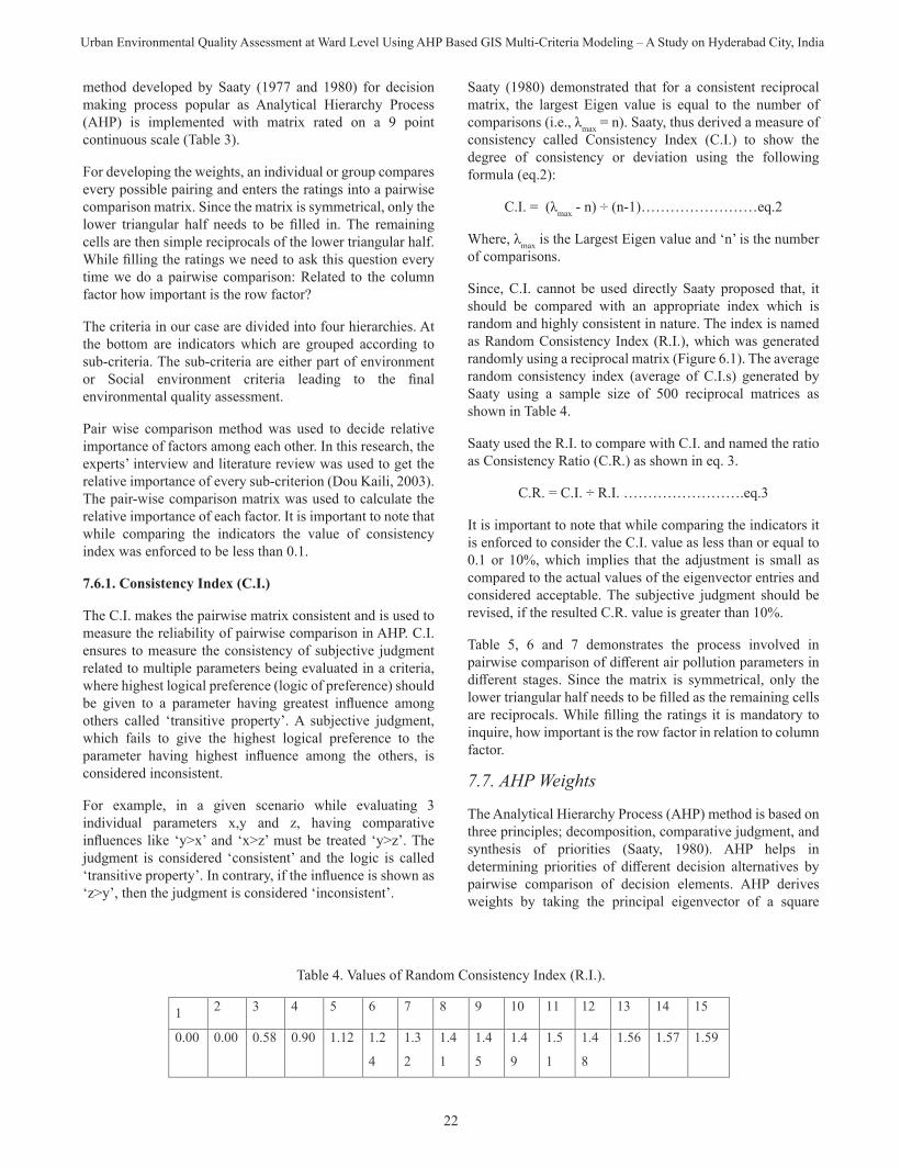
Since, C.I. cannot be used directly Saaty proposed that, it should be compared with an appropriate index which is random and highly consistent in nature. The index is named as Random Consistency Index (R.I.), which was generated randomly using a reciprocal matrix (Figure 6.1). The average random consistency index (average of C.I.s) generated by Saaty using a sample size of 500 reciprocal matrices as shown in Table 4.

Saaty used the R.I. to compare with C.I. and named the ratio as Consistency Ratio (C.R.) as shown in eq. 3.

C.R. = C.I. ÷ R.I. …………………….eq.3

It is important to note that while comparing the indicators it is enforced to consider the C.I. value as less than or equal to 0.1 or 10%, which implies that the adjustment is small as compared to the actual values of the eigenvector entries and considered acceptable. The subjective judgment should be revised, if the resulted C.R. value is greater than 10%.

Table 5, 6 and 7 demonstrates the process involved in pairwise comparison of different air pollution parameters in different stages. Since the matrix is symmetrical, only the lower triangular half needs to be filled as the remaining cells are reciprocals. While filling the ratings it is mandatory to inquire, how important is the row factor in relation to column factor.

7.7. AHP Weights

The Analytical Hierarchy Process (AHP) method is based on three principles; decomposition, comparative judgment, and synthesis of priorities (Saaty, 1980). AHP helps in determining priorities of different decision alternatives by pairwise comparison of decision elements. AHP derives weights by taking the principal eigenvector of a square

(Fig. 6.1). The average random consistency index (average of C.I.s) generated by Saaty using

a sample size of 500 reciprocal matrices as shown in Table 4.

Table 4. Values of Random Consistency Index (R.I.)

1 2 3 4 5 6 7 8 9 10 11 12 13 14 15

0.00 0.00 0.58 0.90 1.12 1.2

4

1.3

2

1.4

1

1.4

5

1.4

9

1.5

1

1.4

8

1.56 1.57 1.59

Source: Saaty, 1980

Saaty used the R.I. to compare with C.I. and named the ratio as Consistency Ratio (C.R.) as

shown in eq. 3.

C.R. = C.I. ÷ R.I. …………………………………………………………….eq.3

It is important to note that while comparing the indicators it is enforced to consider the C.I.

value as less than or equal to 0.1 or 10%, which implies that the adjustment is small as

compared to the actual values of the eigenvector entries and considered acceptable. The

subjective judgment should be revised, if the resulted C.R. value is greater than 10%.

Table 5, 6 and 7 demonstrates the process involved in pairwise comparison of different air

pollution parameters in different stages. Since the matrix is symmetrical, only the lower

triangular half needs to be filled as the remaining cells are reciprocals. While filling the

ratings it is mandatory to inquire, how important is the row factor in relation to column

factor.

Table 4. Values of Random Consistency Index (R.I.).

22

Asian Journal of Geoinformatics, Vol.15,No.3 (2015)

Stage 1: Comparison of Indicators

Table 5. Comparison of Air Pollution Indicators.

(a) Priority Ranking (A) (b) Priority Ranking (A) Values

SO2 NOx TSPM SO2 1 3 1/7 NOx 1/3 1 1/9 TSPM 7 9 1

SO2 NOx TSPM SO2 1.0000 3.0000 0.1429 NOx 0.3333 1.0000 0.1111 TSPM 7.0000 9.0000 1.0000

(c) Normalized A (d) Priority/Eigen Vector (x)

SO2 NOx TSPM SO2 0.1200 0.2308 0.1139 NOx 0.0400 0.0769 0.0886 TSPM 0.8400 0.6923 0.7975

SO2 0.1548 NOx 0.0685 TSPM 0.7765

(e) Ax (f) λmax = average{Ax/x} SO2 0.4714 NOx 0.2064 TSPM 2.4775

SO2 3.0431 NOx 3.0131 TSPM 3.1902

Avg. 3.0821

(g) Consistency Index (C.I.) (g) Consistency Ratio (C.R.) C.I. = (λmax-n)/(n-1) C.I. = (3.0821-3)/(3-1) = 0.04107

C.R. = C.I./R.I. :: for a 2nd order comparison R.I. is 0.58 (Saaty, 1980) C.R. = 0.04107/0.58 = 0.0708 = 7.08% :: 7.08% <10%; the comparison is consistent

Stage 2: Comparison of Sub-Criteria

Table 6. Pairwise Comparison of Natural Environmental Quality Indicators

C.I. = 0.019077 Air

Pollution Water

Pollution Solid

Waste Noise

Pollution X λmax

Air Pollution 1 5 7 3 0.5852 4.1400 Water Pollution 0.2 1 3 1 0.1643 4.0404 Solid Waste 0.1429 0.3333 1 0.3333 0.0661 4.0204 Noise Pollution 0.3333 1 3 1 0.1842 4.0279

C.I. = 0.0190; C.R. = 0.0211 or 2.12% (i.e., <10%)

Table 7. Pairwise Comparison of Urban Landscape Quality Indicators

C.I. = 0.002642 Population Green Spaces

Waterbodies

Relative Entropy

X λmax

Population 1 0.1429 0.1429 1 0.0598 4.0016 Green Spaces 7 1 1 9 0.4437 4.0140 Waterbodies 7 1 1 9 0.4437 4.0140 Relative Entropy 1 0.1111 0.1111 1 0.0528 4.0018

C.I. = 0.0026; C.R. = 0029 or 0.29% (i.e., <10%)

Stage 3: Comparison of Criteria

Table 8. Pairwise Comparison of Natural and Landscape Environments

C.I. = 0 Urban Landscape

Environmental Pollution

X λmax

Urban Landscape Environment

1 0.1429 0.1250 2.0000 Environmental Pollution 7 1 0.8750 2.0000

C.I. = 0.0000; C.R. = 0.0000 or 0% (i.e., <10%)

7.7. AHP Weights

The Analytical Hierarchy Process (AHP) method is based on three principles; decomposition,

comparative judgment, and synthesis of priorities (Saaty, 1980). AHP helps in determining

priorities of different decision alternatives by pairwise comparison of decision elements. AHP

derives weights by taking the principal eigenvector of a square reciprocal matrix of pair wise

comparisons between the criteria to produce best fit set of weights. AHP also results in a

statistical ratio called Consistency Ratio (CR), which indicates the probability of the matrix

ratings which were generated randomly. Pairwise comparison matrix with CR rating >0.1

should be re-evaluated and adjusted to meet the comparison consistency and if the consistent

indicator CR is less than 0.1, the comparison is consistent.

Table 9. AHP Weights and Hierarchies to Determine Urban Environmental Quality

objective Criteria (W) Sub Criteria (W) Indicator (W)

Urb

an E

nvir

onm

enta

l Qua

lity

Nat

ural

Env

iron

men

t (0

.875

)

Air pollution (0.585227)

SO2 concentration (0.154898)

NOx concentration (0.068510)

TSPM concentration (0.776592

Water pollution (0.164367)

Water Quality Index

Solid waste (0.066153) Per capita solid waste

Noise pollution (0.184253) Regional average noise

Urb

an

Lan

dsca

pe

Env

iron

men

t (0

.125

)

Population (0.059815) Population density

Green Spaces (0.443706) % extent of green area in wards

Waterbodies (0.443706) % extent of waterbodies in wards

Relative entropy (0.052773) Sprawl at ward level

When considering the consistent judgment of the pair wise comparison, the comparison

matrix should always be adjusted and the interviews are to be done many times. The weights

for the criterion are determined in two stages. In the first stage, the ranks of the criteria are

reciprocal matrix of pair wise comparisons between the criteria to produce best fit set of weights. AHP also results in a statistical ratio called Consistency Ratio (CR), which indicates the probability of the matrix ratings which were generated randomly. Pairwise comparison matrix with CR

rating >0.1 should be re-evaluated and adjusted to meet the comparison consistency and if the consistent indicator CR is less than 0.1, the comparison is consistent.

When considering the consistent judgment of the pair wise

23

Urban Environmental Quality Assessment at Ward Level Using AHP Based GIS Multi-Criteria Modeling – A Study on Hyderabad City, India

Stage 3: Comparison of Criteria

Table 8. Pairwise Comparison of Natural and Landscape Environments

C.I. = 0 Urban Landscape

Environmental Pollution

X λmax

Urban Landscape Environment

1 0.1429 0.1250 2.0000 Environmental Pollution 7 1 0.8750 2.0000

C.I. = 0.0000; C.R. = 0.0000 or 0% (i.e., <10%)

7.7. AHP Weights

The Analytical Hierarchy Process (AHP) method is based on three principles; decomposition,

comparative judgment, and synthesis of priorities (Saaty, 1980). AHP helps in determining

priorities of different decision alternatives by pairwise comparison of decision elements. AHP

derives weights by taking the principal eigenvector of a square reciprocal matrix of pair wise

comparisons between the criteria to produce best fit set of weights. AHP also results in a

statistical ratio called Consistency Ratio (CR), which indicates the probability of the matrix

ratings which were generated randomly. Pairwise comparison matrix with CR rating >0.1

should be re-evaluated and adjusted to meet the comparison consistency and if the consistent

indicator CR is less than 0.1, the comparison is consistent.

Table 9. AHP Weights and Hierarchies to Determine Urban Environmental Quality

objective Criteria (W) Sub Criteria (W) Indicator (W)

Urb

an E

nvir

onm

enta

l Qua

lity

Nat

ural

Env

iron

men

t (0

.875

)

Air pollution (0.585227)

SO2 concentration (0.154898)

NOx concentration (0.068510)

TSPM concentration (0.776592

Water pollution (0.164367)

Water Quality Index

Solid waste (0.066153) Per capita solid waste

Noise pollution (0.184253) Regional average noise

Urb

an

Lan

dsca

pe

Env

iron

men

t (0

.125

)

Population (0.059815) Population density

Green Spaces (0.443706) % extent of green area in wards

Waterbodies (0.443706) % extent of waterbodies in wards

Relative entropy (0.052773) Sprawl at ward level

When considering the consistent judgment of the pair wise comparison, the comparison

matrix should always be adjusted and the interviews are to be done many times. The weights

for the criterion are determined in two stages. In the first stage, the ranks of the criteria are

Table 9. AHP Weights and Hierarchies to Determine Urban Environmental Quality.

comparison, the comparison matrix should always be adjusted and the interviews are to be done many times. The weights for the criterion are determined in two stages. In the first stage, the ranks of the criteria are decided and in the second stage, the rank of the importance is used to construct the pair wise comparison matrix for AHP. The result of pair wise comparison has AHP weights with a Consistency Index (Table 9).

7.8. Weighted Linear Combination (WLC) for Multi-Criteria Evaluation

Weighted linear combination aggregation method multiplies each standardized factor map by its factor weight and then sums the results. Since the set of factor weights for an evaluation must sum to one, the resulting suitability map must have the same range of values similar to the standardized factor maps that were used. This result is then multiplied by each of the constraints to mask out unsuitable areas. Factor weights are weights that apply to specific factors and indicate the relative degree of importance of each factor plays in determining the suitability. In WLC the weight given to each factor also determines how it wills tradeoff relative to other factors. A factor with a highest weight can tradeoff or compensate for poor scores on other factors, even if the un-weighted suitability score for that factor is not so good. In contrast, a factor with a high suitability score but a small factor weight can only weakly compensate for poor scores on other factors. The factor weights determine how factors tradeoff but, order weights determine the overall level of tradeoff allowed.

7.9. Weighted Linear Combination

Weighted linear combination (WLC) method of aggregation was selected in order to balance the risk and uncertainty in decision making. Apart from this, WLC ensures compensation of factors based on the weights. WLC method was run 4 times to arrive at final Urban Environmental Quality. At first it was performed at indicator level to arrive at sub-criteria.

decided and in the second stage, the rank of the importance is used to construct the pair wise

comparison matrix for AHP. The result of pair wise comparison has AHP weights with a

Consistency Index (Table 9).

7.8. Weighted Linear Combination (WLC) for Multi-Criteria Evaluation

Weighted linear combination aggregation method multiplies each standardized factor map by

its factor weight and then sums the results. Since the set of factor weights for an evaluation

must sum to one, the resulting suitability map must have the same range of values similar to

the standardized factor maps that were used. This result is then multiplied by each of the

constraints to mask out unsuitable areas. Factor weights are weights that apply to specific

factors and indicate the relative degree of importance of each factor plays in determining the

suitability. In WLC the weight given to each factor also determines how it wills tradeoff

relative to other factors. A factor with a highest weight can tradeoff or compensate for poor

scores on other factors, even if the un-weighted suitability score for that factor is not so good.

In contrast, a factor with a high suitability score but a small factor weight can only weakly

compensate for poor scores on other factors. The factor weights determine how factors

tradeoff but, order weights determine the overall level of tradeoff allowed.

7.9. Weighted Linear Combination

Weighted linear combination (WLC) method of aggregation was selected in order to balance

the risk and uncertainty in decision making. Apart from this, WLC ensures compensation of

factors based on the weights. WLC method was run 4 times to arrive at final Urban

Environmental Quality. At first it was performed at indicator level to arrive at sub-criteria.

Sub-criteria were further subjected to WLC in order to get Criteria. Finally Criteria were

aggregated using WLC to arrive at final Urban Environmental Quality at ward level in

Hyderabad. This hierarchical approach ensured the weights given to individual indicator, sub-

criteria and criteria to influence the final result.

WLC is the most commonly used decision method and represented mathematically in eq.4.

S = ∑ wi xi ∗ cj . . . . . . eq.4

Where, S is the composite score; wi is the AHP weight assigned to each factor to indicate

relative importance of the participating parameters over other (total weights of all parameters

must equal to 100 percent); xi is the factor or feature class score indicates the significance of

the class within the theme (in case of qualitative classes the classes would be assigned with

scores in the form of a geometric progression like 1, 2, 4, 8…n or on a scale of 1-10; Π is the

Sub-criteria were further subjected to WLC in order to get Criteria. Finally Criteria were aggregated using WLC to arrive at final Urban Environmental Quality at ward level in Hyderabad. This hierarchical approach ensured the weights given to individual indicator, sub-criteria and criteria to influence the final result.

WLC is the most commonly used decision method and represented mathematically in eq.4.

Where, S is the composite score; wi is the AHP weight assigned to each factor to indicate relative importance of the participating parameters over other (total weights of all parameters must equal to 100 percent); xi is the factor or feature class score indicates the significance of the class within the theme (in case of qualitative classes the classes would be assigned with scores in the form of a geometric progression like 1, 2, 4, 8…n or on a scale of 1-10; Π is the product of constraints (1- suitable and and 0 – unsuitable); Cj is the constraints or boolean factors like waterbodies, sensitive zones, protected areas, elevation etc.

Total Score = (criteria1*weight1) + (criteria2*weight2) + (criterian*weightn) ..eq.5

The integration of themes is done at different levels of hierarchies as shown in eq.5.

7.9.1 Decision Making

Evaluation analysis of environment quality results in an output of quality ranked wards and a decision is to be made based on certain criteria with a choice between alternatives of different courses of action. The decision frame for an environmental quality evaluation might be different categories like ‘good’, ‘moderate’ and ‘poor’. However, it should be distinguished from the individuals to whom the decision is being applied and is called a ‘candidate set’ which

24

Asian Journal of Geoinformatics, Vol.15,No.3 (2015)

Figure 3. Urban Environmental Quality – Continuous.

Figure 4. Urban Environmental Quality - Ward based Averaged Values.

25

Urban Environmental Quality Assessment at Ward Level Using AHP Based GIS Multi-Criteria Modeling – A Study on Hyderabad City, India

is a set of locations that can be zoned. Finally, decision sets which represent set of all individuals that are assigned a specific alternative or areas having identical values from the decision frame were derived. As such decision sets constituting decision candidates such as very good, good, moderate and poor environmental quality were assigned as a choice of alternative characterizations for an individual.

8. Results and Discussion

In order to assess the urban environmental quality of the GHMC, various environmental indicators were analyzed using AHP based weights and the results were grouped into 5 categories from 1 (Very good quality) to 5 (Bad quality). The results were grouped into 5 classes, because they make it possible to show the results in minimum classes distinctively with maximum variance. The values classified are in the range of 1.92 to 4.16. The spatial trend of the values shows that the environment quality scenario in the eastern and central regions of GHMC is worst, while the west, north and south-west regions are shows a good environment quality. Regions on the outskirts and fringe areas of the city show the best urban environmental quality as expected (Figure 3 and 4).

Interpretation of mapping results (Figure 4), indicates that out of 150 wards majority (138) wards in Hyderabad (GHMC) are classified into classes indicating deteriorated environmental quality conditions, by getting classified into either, ‘Bad’ or ‘Poor’ or ‘Moderately Good’. Very few wards (only 12) have got classified as either ‘Good’ or ‘Very Good’ in terms of overall environmental quality. Majority of wards (85) have got classified as ‘Bad’ with deteriorated

overall environmental conditions. These wards comprises of 3,041,551 (56.21%) population covering an area of 191.58km2 (31.41%) with high density. Some of the wards include Uppal, L. B. Nagar, Gaddi Annaram, I.S. Sada, Chandrayana Gutta, Old Malakpet, Moghalpura, Falaknuma, Shalibanda etc. belongs to south, central, north and east zones. A total of 29 wards have been categorised as ‘Moderately Good’ with a population of 1,069,242 (19.76%) with an area coverage of 157.68km2 (25.85%). Some of the wards in this category are Shivarampally, Mylardevpally, Panjagutta, Somajiguda, Srinagar Colony, Banjara Hills, Erragadda, Vengalrao Nagar, Fethe Nagar, Old Bowenpally, Gajularamaram, Jagadgirigutta etc. belongs to central, west or north zones. The 3rd major environmental quality category is ‘Poor’ with 24 wards covering an area of 109.97km2 (18.03%) with a population of 859,461(15.88%). Some of the prominent wards in this category are Cherlapalli, Mallapur, Fathe Darwaza, Ramnaspura, Gudimalkapur, KPHB Colony, Hydernagar, Suraram Colony, Old Malkajgiri, Begumpet etc. mostly belongs to south, north and west zones. A total of 8 wards comprising 298753 (5.52%) of population covering an area of 130.92km2 (21.46%) have been categorised as ‘Good’ indicating a sound environmental quality scenario. The remaining 4 wards have got categorised as ‘Very Good’ with high levels of overall environmental quality. These wards are Yousufguda (central zone), Kishanbagh, Rahmath Nagar and Jubilee Hills (south zone) have a population of 142,524(2.63%) with an area of 19.8km2(3.25%). The wards categorised as either ‘good’ or ‘Very Good’ are mostly confined to the fringe areas, except (Jubilee Hills) of the city with low density of population and most green areas and waterbodies. Whereas, jubilee Hills

Figure 5. Economic Growth Centers of Hyderabad.

26

Asian Journal of Geoinformatics, Vol.15,No.3 (2015)

with its peculiar undulated terrain is still intact with sustainable environmental quality due to prevailing socio-economic and terrain conditions.

9. Approach for Sustainable Development and Environmental Management

Keeping in view of the environmental quality results obtained a site suitability analysis was conducted to locate appropriate sites for development in the city guided by the intent to minimize the possible adverse effects and cost of development on the environment as well as on existing communities. This also emphasizes the positive impacts of such development by locating them in a most suitable location. This is achieved by examining different alternative individual by assigning them with relative importance (criteria) as a whole and using a mathematical model to identify the most suitable location.

This is done by assigning values to the individual parameters (on a relative scale of 1 to 10), the process termed as ranking. The ranks assigned are in accordance with the importance for determining locations suitable for economic prosperity. Subsequently, the criteria within each class of the parameter or theme is assigned with respective weights within the range of 1 to 10. The basic difference between a rank and a weight is only that the rank is applied across different data layers, whereas weight is applied within a data layer. The list of data themes used for site suitability analysis is transport (road, railway etc.), land use (residential, industrial, green spaces and open spaces etc.), economic growth potential zones, population density, entropy and overall urban environmental quality.

The final suitability map has different zones displayed in a gradation of red to green (Figure 5). The green patches represent the most favourable locations for industrial or economic development, whereas coloured in red denote the least suitable areas. From the Figure 5, it can be noticed that class 1 followed by class 2, 3 and 4 represented in green are considered most favourable zones for the development and economic activities. Classes 10, 9, 8 and 7 shown in red are considered not favourable for any economic activity, as most of these areas comes under existing built-up/residential zones.

Traditional economic sectors like manufacturing have always been a foremost driver for urban growth. However, these activities are considered as significant suppliers of environmental contamination. Keeping this in view, the analysis has identified areas on the fringe zones of the city, such as Ramachandrapuram, Patancheru, Balanagar, Uppal, Cherlapalli, Jeedimetla and Moula Ali, which are now being considered as most happening places found suitable for manufacturing as they provide a mesh of associated commerce.

10. Measures to Enhance Urban

Environmental Quality

Based on the environmental quality and site suitability analysis results, the study recommends various measures to enhance the environmental quality without effecting the on-going developmental activities. The various functional measures recommended for implementation are:

Air quality control measures: (a) encourage green technologies (solar, hydrogen, electric, wind, bio-fuel as alternative fuel) (b) use unleaded petrol and fuels low with sulphur and ash content (c) encourage people to use public transportation systems (d) plan and implement green belts (e) restrict emissions in industries to permissible limits (f) make it mandatory to use the air pollution control equipment in all industries, etc.

Water quality control measures: (a) minimize water pollutant generation, (b) treat the polluted water prior to disposal, and (c) ‘in-situ’ reduction or elimination of pollution etc.

Noise pollution control measures: (a) control noise at source level using modern technology/devices (b) install sound insulators while constructing the structures (c) control noise at receivers end using necessary gadgets available in the market (d) create the acoustic zones especially for public areas (e) plant trees along the transportation corridors (appropriate policy measures restricting the sound levels at appropriate zones (hospitals, residential areas, schools etc.).

Solid waste management measures: (a) reduce the volume of the waste being generated (b) reuse the waste (c) recycle the waste etc.

Slum growth management measures: (a) monitor the growth of unwarranted habitats (b) recognise the rights of urban poor and help them to improve the socio-economic conditions (c) provide housing to below poverty line (BPL) population (d) improve the condition of existing slums and infrastructure.

11. Conclusions

The study based on AHP and GIS using MCE provides an ideal framework for effectively evaluating and rating the municipal wards of GHMC which involves integration and analysis of multiple factors and varied biases. Based on the results obtained from the analysis it is noticed that the environmental quality is still intact in outskirts of the GHMC where urban growth is not yet intense and due to the presence of more green areas. Wards with good urban environmental quality are found along the areas where urban areas are still sparse. However, these areas are also undergoing rapid development due to sprawl and have the potential to grow in the near future. Therefore it is important to prioritize these areas to keep them environmentally compliant and to prevent from further deterioration. Through AHP-MCE based GIS

27

Urban Environmental Quality Assessment at Ward Level Using AHP Based GIS Multi-Criteria Modeling – A Study on Hyderabad City, India

References

Anjali, A., Chauhan, S.S., Goyal, S.K. 2011. A multi-criteria decision making approach for location planning for urban distribution centers under uncertainty, Mathemetical and Computer Modelling, Vol. 53, 98-109.

Chinag, C. and Lai, C. 2002. “A study on the comprehensive indicator of indoor environment assessment for occupant’s health in Taiwan, Building and Envi., Vol. 37, 387-392.

Chokor, B.A. 1989. The Evaluation of Envi. Quality for Planning in the Third World, Third World Planning Review, Vol. 11(2), 189-210.

Dou Kaili 2003. Fuzzy evaluation of urban environmental quality, case study Wuchang, Wuhan, Masters Thesis submitted to International Institute for Geo-information Science and Earth Observation, Enschede, The Netherlands, ITC. https://www.itc.nl/library/papers_2003/msc/upla/dou.pdf

Feiring, R. (1986) - Linear Programming: An Introduction, Quantitative - Applications in the Social Sciences, Sage Publications, London, Vol. 60.

Ignizio, J.P. 1985. Introduction to Linear Goal Programming,

Sage Publications, CA.

Klungboonkrong, P. and Taylor, M.A.P. 1998. A Microcomputer-based System for Multi-Criteria Environment Impacts Evaluation of Urban Road Network Computation, Envi. & Urban Sys., Vol. 22(5), 425-446.

Lee, K.L.G. and Chan, E.H.W. (2008) - The Analytic Hierarchy Process (AHP) Approach for Assessment of Urban Renewal Proposals, Soc. Indic. Res., Vol. 89, 55-168.

Mouna Ketata-Rokbani, Moncef, G. and Rachida, B. 2011. Use of GIS and Water Quality Index to Assess Groundwater Quality in El Khairat Deep Aquifer (Enfidha, Tunisian Sahel), Iranica Journal of Energy & Envi., Vol. 2(2), 133-144.

Munda, G.P. and Nijkamp 1994. Qualitative Multicriteria Evaluation for Environmental Mgmt., Ecological Economics, Vol. 10(2), 97-112.

Odemerho, F.O. and Chokor, B.A. 1991. An Aggregate Index of Environmental Quality: the Example of a Traditional City in Nigeria, Applied Geography, Vol. 11(1), 35-58.

Quaddus, M.A. and Siddique, M.A.B. 2001. Modeling Sustainable Development Planning: A Multicriteria Decision Conferencing Approach, Envi. International, Vol. 27, 89-95.

Rapoport, A. 1983. Environmental Quality, Metropolitan Areas and Traditional Settlements. Habitat Intl. Vol. 7(3/4): 37-63.

Saaty, T.L. 1977. “A Scaling Method for Priorities in Hierarchical Structures”, Journal of Mathematical Psychology, Vol. 15, 234-281.

Saaty, T.L. 1980. The analytic hierarchy process. Polytechnic University of Hochiminh city, Vietnam McGraw-Hill, New York.

Sharifi, A. and Herwijnen, M.V. 2003. Spatial Decision Support Systems, Int. Inst. for Geo-Info. Sci. & Earth Observation (ITC). 201.

Tzeng, G.H., Teng, M.H., Chen, J.J. and Opricovic, S. 2002. Multicriteria Selection for a Restaurant Location in Taipei, Int. Journal of Hospitality Mgmt., Vol. 21(2), 171-187.

Xu, X.Q. 1989. A Factorial Ecological Study of Social Spatial Structure in Guangzhou, ACTA Geographical Sinica, Vol. 44(4), 385-399.

Xu, Z. 1999. Urban environment planning, Wuhan. Wuhan technical University of Surveying and Mapping Press.

analysis, the study helped in identifying the urban areas/wards with bad/poor environmental quality which needs immediate attention for improvement. The wards finally identified with ‘Bad’ or ‘Poor’ environmental quality are in fact repeatedly classified as ‘Bad’ or ‘Poor’ across various quality parameters (air, water, noise, solid waste, green areas etc.). Identification of such wards is in a way greatly helps the city administrators to keep focus on them instead developing the wards based on a single quality measure. This also makes it easier to address the common problems which deteriorate the quality of environment in these urban pockets. In order to enhance the environmental quality of the wards categorized as ‘Bad’ or ‘Poor’ various functional measures are recommended for implementation. Keeping the environmental quality results as premise a site suitability analysis was carried out using GIS to locate the favorable sites for economic development. Incidentally, various measures have been recommended to enhance the environmental quality of the zones identified with deteriorated conditions. The AHP-GIS based MCDM analysis model implemented in this study is of prime importance for smart-city initiatives being taken by the governments as this make it possible to properly plan and prioritize the resources and areas being developed based on multiple factors influencing the urban setup.

28

Asian Journal of Geoinformatics, Vol.15,No.3 (2015)

Wang, S.B. 2002. The Mixed Welfare System and Development of Social Capital of the Vulnerable Groups, China Social Work Research, 1: 13-23.

Ying, L.G. and Kung, H.T. 2000. Forecasting up to year 2000 on Shanghai’s environment quality, Environment Monitoring and Assessment, 63: 297-312.

29

View publication statsView publication stats