MULTI-CHANNEL RETAILING WITH PRODUCT …etd.lib.metu.edu.tr/upload/12618472/index.pdf · i multi-channel retailing with product differentiation a thesis submitted to the graduate

i

MULTI-CHANNEL RETAILING WITH PRODUCT DIFFERENTIATION

A THESIS SUBMITTED TO

THE GRADUATE SCHOOL OF NATURAL AND APPLIED SCIENCES

OF

MIDDLE EAST TECHNICAL UNIVERSITY

BY

HAVVA GÜLÇİN UĞUR

IN PARTIAL FULFILLMENT OF THE REQUIREMENTS

FOR

THE DEGREE OF MASTER OF SCIENCE

IN

INDUSTRIAL ENGINEERING

FEBRUARY 2015

ii

iii

Approval of the thesis:


submitted by HAVVA GÜLÇİN UĞUR in partial fulfillment of the requirements

for the degree of Master of Science in Industrial Engineering Department,

Middle East Technical University by,

Prof. Dr. Gülbin Dural Ünver

Dean, Graduate School of Natural and Applied Sciences _____________

Prof. Dr. Murat Köksalan

Head of Department, Industrial Engineering _____________

Assist. Prof. Dr. Özgen Karaer

Supervisor, Industrial Engineering Dept., METU _____________

Examining Committee Members:

Assoc. Prof. Dr. İsmail S. Bakal

Industrial Engineering Dept., METU _____________

Assist. Prof. Dr. Özgen Karaer


Assoc. Prof. Dr. Pelin Bayındır


Assoc. Prof. Dr. Seçil Savaşaneril


Assist. Prof. Dr. Emre Nadar

Industrial Engineering Dept., Bilkent University _____________

Date: 02.02.2015

iv

I hereby declare that all information in this document has been obtained and

presented in accordance with academic rules and ethical conduct. I also declare

that, as required by these rules and conduct, I have fully cited and referenced

all material and results that are not original to this work.

Name, Last Name : Havva Gülçin Uğur

Signature :

v

ABSTRACT


Uğur, Havva Gülçin

M.S., Department of Industrial Engineering

Supervisor: Assist. Prof. Dr. Özgen Karaer

February 2015, 121 pages

In this study, we analyze a monopolist retailer’s product differentiation problem in a

multi-channel environment. We investigate the type of conditions that would

motivate retailer to open an outlet branch, to open an online channel, and to even

potentially open an online channel for the outlet branch, and how these decisions

interact with each other. We use quality and price as the primary drivers in the outlet

business decision in a vertical differentiation model. In the outlet business decision,

specifically, we investigate the quality and price decision of the retailer for his outlet

branch and whether he will be better off in terms of total profit. For the online

channel, we determine the online service quality and other factors that affect the end-

consumer’s utility. Online service quality may involve all customer services

provided by the online store, the convenience of return process, and promised

delivery time windows as well as shipping charges.

We find that the retailer’s decision hinges on the market expansion versus

market/margin cannibalization. We show that even a direct channel for the outlet

store may be preferable for the retailer, depending on the market characteristics.

vi

Keywords: (vertical) product differentiation, multi-channel retailing, outlet business,

online channel, joint online channel and outlet business

vii

ÖZ

ÜRÜN FARKLILAŞTIRMA İLE ÇOK KANALLI PERAKENDE YÖNETİMİ

Uğur, Havva Gülçin

Yüksek Lisans, Endüstri Mühendisliği Bölümü

Tez Yöneticisi: Yar. Doç. Dr. Özgen Karaer

Şubat 2015, 121 sayfa

Bu çalışmada tekelci bir perakandecinin ürün farklılaştırma problemini çok kanallı

satış yapılabilen bir ortamda inceliyoruz. Perakendeciyi outlet açmaya, internet gibi

direkt bir kanal açmaya hatta bu kanal üzerinden üzerinden outlet ürünü satışı

yapmaya teşvik eden ortamları ve bunların birbiri ile etkileşimlerini araştırıyoruz.

Outlet zincirle normal mağazalar arasındaki temel fark fiyat ve kalite olarak ele

alınmıştır. Bu aşamada, ürünün fiyat ve kalite açısından konumlandırılmasını,

bununla birlikte perakendecinin karındaki değişikliği inceliyoruz. İnternet kanalı için

internet hizmet kalitesini ve müşteri memnuniyetini etkileyecek faktörleri

inceliyoruz. İnternet hizmet kalitesi internet üzerinden sağlanan müşteri hizmetleri,

iade, öngörülen sürede teslim ve teslimat ücretlendirmesini de kapsamaktadır.

Perakendecinin kararının pazar payı artışı ve diğer kanallardaki pazar ve kar marjı

kaybı arasındaki ödünleşmeye dayandığını bulduk. İnternet outlet mağazası

perakendeci için kazançlı olabileceğini ancak pazar özelliklerine de bağlı

olabileceğini gösterdik.

viii

Anahtar Kelimeler: dikey ürün farklılaştırma, çok kanallı perakendecilik, outlet,

internet üzerinden satış, internet üzerinden outlet ürünü satışı

ix

To my dear family;

x

ACKNOWLEDGEMENTS

I would like to express my deepest appreciation to Dr.Özgen Karaer for her

wholehearted support, understanding and help throughout the development of this

thesis study. Without her patience and help this study could not have been

completed. I also want to thank all academic staff in the department for their support

and motivation they gave whenever I need.

I really appreciate the support and motivation of my dearest friend Derya Taşçı and

Ali Ayturan who were always there. With their love and understanding I managed to

overcome the difficulties in the process.

Finally, I would like to express my deepest thanks to my parents Emine and Ali Uğur

for their endless love, trust, understanding and every kind of support not only

throughout my thesis but also my life and to M.Oluş Özbek for every kind of support

and being with me all the time.

xi

TABLE OF CONTENTS

ABSTRACT ................................................................................................................. v

ÖZ .............................................................................................................................. vii

ACKNOWLEDGEMENTS ......................................................................................... x

TABLE OF CONTENTS ............................................................................................ xi

LIST OF TABLES .................................................................................................... xiii

LIST OF FIGURES .................................................................................................. xiv

CHAPTERS

1. INTRODUCTION ............................................................................................... 1

2. LITERATURE SURVEY .................................................................................... 5

3. THE PHYSICAL OUTLET DECISION OF THE BRICK-AND-MORTAR

RETAILER ............................................................................................................ 15

3.1 The Physical Outlet Decision of the Brick-and-Mortar Retailer without

Inconvenience Cost ............................................................................................ 15

3.1.1 Myopic Retailer ..................................................................................... 25

3.1.2 Non-Myopic Retailer ............................................................................ 26

3.2 The physical outlet decisions of a brick-and-mortar retailer with

inconvenience cost ............................................................................................. 29

3.3 Numerical analysis on the outlet decisions with inconvenience costs ......... 38

4. ONLINE CHANNEL DECISION FOR A BRICK-AND-MORTAR

RETAILER ............................................................................................................ 47

5. ONLINE CHANNEL DECISION FOR A BRICK-AND-MORTAR

RETAILER WITH AN OUTLET BRANCH ........................................................ 59

xii

5.1 The optimal online service under Case 1 (θ1≤θ2≤θ*) ................................... 65

5.2 The optimal online service under Case 2 (θ1>θ2>θ*) ................................... 70

6. JOINT ONLINE CHANNEL AND OUTLET BUSINESS .............................. 77

7. CONCLUSION .................................................................................................. 95

REFERENCES ....................................................................................................... 99

APPENDICES

A. NUMERICAL ANALYSIS FOR TRIAL 2 .................................................... 101

B. NUMERICAL ANALYSIS FOR TRIAL 1 .................................................... 105

C. NUMERICAL ANALYSIS FOR THE FIRST GROUP TRIALS ................. 109

D. NUMERICAL ANALYSIS FOR THE SECOND GROUP TRIALS ............ 111

E. LEMMA 4.2 .................................................................................................... 113

F. PROPOSITION 5.4 ......................................................................................... 115

G. PROPOSITION 5.5 ......................................................................................... 117

H. PROOF OF PROPOSITION 6.2 ..................................................................... 119

I. PROOF OF PROPOSITION 6.3 ...................................................................... 121

xiii

LIST OF TABLES

TABLES

Table 3.1: Notation..................................................................................................... 16

Table 3.2: Comparing “only primary business“ and “with an outlet branch “ cases on

profit and consumer surplus ............................................................................... 22

Table 3.3: Comparing “only primary business” and “with an outlet branch “cases on

profit, demand, price and quality level of the products...................................... 24

Table 3.4: The primary brand position and the total profit in the “myopic” and “non-

myopic” retailer cases ........................................................................................ 29

Table 3.5: Notation..................................................................................................... 31

Table 3.6: The parameters of the example ................................................................. 35

Table 3.7: The leading principal minors for some (s2, p2) values .............................. 35

Table 3. 8: The first and second group of trials ......................................................... 38

Table 4.1: Notation..................................................................................................... 49

Table 4.2: The comparisons between “only physical chain” and “both online and

physical chain” ................................................................................................... 57

Table 5.1: Notation..................................................................................................... 61

Table 5.2: The retailer’s total profit, market condition and the optimal delivery time

under Case 1 and 2 ............................................................................................. 76

Table 6.1: Notation..................................................................................................... 79

Table 6.2: Threshold values and orders of all options under Case 1 of Chapter 5 and

6 ......................................................................................................................... 92

Table 6.3: Threshold values and orders of all options under Case 2 of Chapter 5 and

6 .......................................................................................................................... 93

Table A. 1: s2*, p2

*, D1

*, D2

* retailer’s profit and total market and profit margin of

the outlet for trial 2 when k=0.5 ....................................................................... 101

Table B.1: s2*, p2

*, D1

*, D2

* ,retailer’s profit for trial 1 when m=k .......................... 105

xiv

LIST OF FIGURES

FIGURES

Figure 3.1: The demand of the retailer before (a) and after (b) the introduction of the

outlet branch (and its split between channels) ................................................... 18


outlet branch (and its split between channels) ((p1-p2+k-m)/(s1-s2) b) ............ 33

Figure 3.3: s2* versus m plot for trial 2 when k=0.5 .................................................. 39

Figure 3.4: p2* versus m plot for trial 2 when k=0.5 .................................................. 39

Figure 3.5: Retailer’s profit versus m plot for trial 1 when m=k ............................... 40

Figure 3.6: p2* for the first group of trials when k=0.3 .............................................. 41

Figure 3.7: s2* for the first group of trials when k=0.3 .............................................. 42

Figure 3.8: D2* for the first group of trials when k=0.3 ............................................. 42

Figure 3.9: s2* for the second group of trials when k=0.3 .......................................... 43

Figure 3.10: p2* for the second group of trials when k=0.3 ....................................... 44

Figure 3.11: D2* for the second group of trials when k=0.3 ...................................... 44

Figure 4.1: Total demand after the introduction of the online channel (and its split

among channels)................................................................................................. 51

Figure 4.2: Profit change and optimal online service with respect to online service

cost (Order 1) ..................................................................................................... 58


cost (Order 2) ..................................................................................................... 58


online channel (and its split among channels) under Case 1 ............................. 64


online channel (and its split among channels) under Case 2 ............................. 65

xv

Figure 6.1: Retailer’s demand after the introduction of the online outlet (and its split

among channels) under Case 1 (where θ=(p1-p2)/(s1-s2)) .................................. 82


among channels) under Case 2 when θ1>θ2>θ3>θ* (a) and θ1>θ2>θ

*>θ3 (b)

(where θ=(p1-p2)/(s1-s2)) ..................................................................................... 82

Figure A.1: D1* versus m plot for trial 2 when k=0.5 .............................................. 102

Figure A.2: D2* versus m plot for trial 2 when k=0.5 .............................................. 103

Figure A.3: Retailer’s profit versus m plot for trial 2 when k=0.5 .......................... 103

Figure A.4: Retailer’s total market share versus m plot for trial 2 when k=0.5....... 104

Figure A.5: (p2-c(s2*)2) versus m plot for trial 2 when k=0.5 .................................. 104

Figure B.1: s2* versus m plot for trial 1 when m=k .................................................. 107

Figure B.2: p2* versus m plot for trial 1 when m=k ................................................. 107

Figure B.3: D1* versus m plot for trial 1 when m=k ................................................ 108

Figure B.4: D2* versus m plot for trial 1 when m=k ................................................ 108

Figure C.1: D1* for the first group of trials when k=0.3 ........................................... 109

Figure D.1: D1* for the second group of trials when k=0.3 ..................................... 111

Figure D.2: Retailer’s market share for the second group of trials when k=0.3 ...... 111

Figure F.1: t*, ∆∏5.1 for Order 1 under Case 1 ......................................................... 116

Figure F.2: t*, ∆∏5.1 for Order 2 under Case 1 ........................................................ 116

Figure G.3: t*, ∆∏5.2 for Order 1 under Case 2 ........................................................ 118

Figure G.4: t*, ∆∏5.2 for Order 2 under Case 2 ........................................................ 118

Figure H.1: t*, ∆∏5.1, ∆∏6.1 when (p1-c1

2)-(p2-s2

2)<0 .............................................. 119

Figure H.2: t*, ∆∏5.1, ∆∏6.1 when (p1-c1

2)-(p2-s2

2)>0 and zlimit 6.1<0 ....................... 119

Figure H.3: t*, ∆∏5.1, ∆∏6.1 for Order (1) ................................................................ 119

Figure H.4: t*, ∆∏5.1, ∆∏6.1 for Order (2) ................................................................ 120

Figure H.5: t*, ∆∏5.1, ∆∏6.1 for Order (3) and Order (4) ......................................... 120

Figure I.1: t*, ∆∏5.2, ∆∏6.2 for Proposition 6.3(ii) .................................................... 121

Figure I.2: t*, ∆∏5.2, ∆∏6.2 for Proposition 6.3(iii) ................................................. 121

xvi

1

CHAPTER 1

INTRODUCTION

Berman and Evans (2006) define a factory outlet store as a manufacturer-owned and

operated store selling closeouts, excess inventory, cancelled orders. Lately, they have

started to offer in-season products as well. The factory outlet as a concept has

evolved over time and has become a business opportunity not for manufacturers but

also specialty retailers and some third-party retailers alike.

Recently, factory outlets started to draw out attention due to different reasons. The

main role of the outlet store has been to liquidate excess inventory. Although prices

are below regular retail prices, outlet stores can generate handsome profits thanks to

low operating cost; i.e., low rent, service standards, and plain store layout. However,

nowadays, outlet stores, parallel to traditional stores, turn into alternative sales

channels that offer a lower quality option of the original collection. For example,

North Face manages the outlet store to liquidate inventory whereas Coach, Ann

Taylor, Guess and J.Crew design its own line for the outlet business (Levy and

Weitz, 2012). In J.Crew, for example, “all J.Crew Factory items are exclusive

designs and based on past J. Crew collection” (accessible via

www.jcrew.com/help/about jcrew.scp). Brooks Brothers (apparel), Levi’s (apparel),

Liz Claiborne (apparel), Samsonite (luggage) also manage their own specialty store

chain alongside their outlet stores. In this respect, outlet business branch represents

an opportunity to expand the market of a retailer brand through vertical

differentiation.

Outlet stores are generally located far from city centers; i.e., mainly in areas of low

real estate market and also in touristic regions. As of 2006 in the U.S., there were

http://www.jcrew.com/help/about%20jcrew.scp

2

16,000 outlet stores clustered in 225 outlet malls, with total annual revenue of

$16,000. (Berman and Evans, 2006)

Direct selling channels, as an alternative to the brick-and-mortar stores, include

catalog business, online stores and mobile stores. As the use of Internet and smart

phones increases every day, multichannel retailing, especially the online channel, is

starting to represent a significant portion of sales. From the viewpoint of the retailer,

online retailing has many advantages. Online channel facilitates easy expansion of a

chain, overcoming the limitations of its brick-and-mortar network – if there are any.

Essentially, online channel provides a retailer means for reaching more customers,

and potentially serving them through a wider assortment. The customer, in the

meantime, is free of the physical inconvenience of the visit and the risk of out-of-

stock that he may face at the store. However, with online purchases, the customer has

to endure the risks such as those associated with the fit, color, and fabric of the

product. Most important, immediate gratification is not possible anymore; the

customer has to patiently wait for his product in addition to other risks associated

with buying online (credit card use and risk, wrong shipments, and etc.). Thus,

online channel, compared to the physical channel that is available, rids the customer

of the physical inconvenience of visiting the store and hence (potentially) expands

retailer’s total market. Especially in apparel and general merchandise, outlet business

branches and online stores are active revenue-generators for a retailer.

Gap Inc. is one of the multi-brand and multi-channel retailers in the apparel industry.

The company conducts retail activities through its online channel in addition to the

physical stores under the Gap, Old Navy, Banana Republic, Piperlime and Athleta

brands. Additionally, Gap and Banana Republic serve their consumers not only

through the physical and online store but also outlet stores under names “Gap Outlet”

and “Banana Republic Factory Store”, respectively. J.Crew, founded in 1983, is a

multi-channel specialty retailer. Now, the firm is reaching more than 100 countries

through the online channel and overseas bricks-and-mortar stores. In addition to

these channels, J.Crew has been serving his consumers with outlet stores named

“J.Crew Factory” since 1988. The other example in the apparel industry is

Nordstrom. It serves its customers with full-line stores, outlet stores as Nordstrom

Rack and online channel via shop.nordstrom.com.

3

Recently, we observe retailers with outlet branches and online stores making their

outlet stores available online as well – basically opening a second channel for their

“value” (low quality, low price) business. Nordstrom’s e-commerce site

Nordstromrack.com provides its consumers to off-price fashion products online. REI

is a category specialist that sells outdoor gears, outdoor goods and accessories

through 131 stores. Also, REI offers its consumers both options of “Shop REI” and

“Shop REI Outlet” in its e-commerce site www.rei.com.

In this thesis, we study the outlet branch and online channel decisions of a retailer,

and their interrelations. We also evaluate the profit implications of an online channel

for the outlet branch. We build our study sequentially by analyzing the cases below.

a. outlet branch decision of a retailer

In Chapter 3, we address the outlet branch decisions of a retailer that currently has a

bricks-and-mortar chain. Note that here the outlet brand represents an inferior

product compared to the original brand both in terms of quality and price.

b. online channel decision of a retailer

In Chapter 4, we address the online channel decision of a retailer with a bricks-and-

mortar chain devoted to his primary brand. Particularly, we investigate the online

services that he provides, and whether he will be better off in terms of total profit and

market expansion. Here, online services include but are not limited to the promised

delivery time (and shipping services) offered by the online store.

c. online channel decision for the primary brand of a retailer that has primary and

outlet branches

In Chapter 5, we are interested in the online store decision of the retailer when the

retailer has already a physical chain of primary brand stores and another that belongs

to the outlet branch.

d. online channel decision for the outlet branch of a retailer that has already a

primary brand with the physical and online channel and an outlet physical channel

In Chapter 6, we address the outlet online channel decision of the multi-channel

retailer.

4

In each chapter (except the last one), we analyze the optimal decisions of the retailer

and the change in his total profit. In Chapter 6, we again evaluate the profit impact of

opening the online outlet store.

Before we present our analysis for each case, we discuss the relevant literature in

Chapter 2. Finally, we conclude in Chapter 7 summarizing our major findings and

offering further research directions.

5

CHAPTER 2

LITERATURE SURVEY

In this work, we study a monopolist retailer’s channel decisions jointly with his

vertical product differentiation strategy. In this respect, our work is closely related

with two streams of research: (vertical) product differentiation and retailer channel

management.

Product differentiation enables a firm to identify and focus on a target consumer

segment. Later, the firm distinguishes its product or service from similar goods and

services which are already offered by competitors to the defined consumer segment.

Therefore, by launching a distinguished good and service the firm may not only

generate more profit but also expand market share. In some cases, product

differentiation may be a strategic necessity for firms.

Shy (1997) categorizes product differentiation models in three main groups which

are “goods-characteristics” approach, non-address approach, and address (location)

approach. In “goods-characteristics” approach, each product can be defined as a sum

of attributes i.e.; color, size etc. and while purchasing, the consumer prefers the

product that consists of the most suitable characteristics for him.

In non-address approach, a higher level in a preferred attribute generates more

demand for the provider firm. The underlying assumption here is, “all consumers

gain utility from consuming a variety of products and therefore buy a variety of

products.” (Shy, 1997) However, in location approach, each consumer buys a

maximum of one product and consumers are heterogeneous in their preferences. In

this approach, location as a concept has two different meanings. One of them is the

physical distance between the consumer and the firm. In this case, the consumer

evaluates the prices of product in all stores and decides where to purchase, taking

6

distance into account as well. The other meaning is that the distance between

consumer’s ideal preference (taste) for the particular good and product at hand. The

consumer’s disutility from buying the less-than-ideal brand which is equivalent to

the transportation cost in the previous case can be interpreted as distance here.

In horizontal product differentiation as a “Location Model”, all consumers in the

market do not have the same order preferences for products. The choice of the

consumer depends on the preference of the particular consumer as well as prices.

The typical example is color; the preference of product color varies in the

population. Location is another example; when the firms are located in the same

street, each consumer that lives on the street will rank the firms differently –

depending on where they live. In the horizontal product differentiation, the consumer

prefers the product closest to him (or his taste) to gain higher utility given the same

prices.

In contrast to horizontal differentiation model, all consumers have the same order

preferences for products in the vertical product differentiation model. For a given

(equal) price, all consumers prefer the same product in vertical differentiation. Put it

differently, when the firms are assumed to locate on a linear street with length of 1,

ideal brand of all consumers are located at point 1. For example, holding all else

constant, all consumers prefer a fuel-efficient Hybrid car to a regular car that runs on

gas. Quality is a typical dimension that firms utilize to vertically differentiate. Here,

quality represents any characteristic of product (or brand) which all consumers prefer

more to less, ceteris paribus, such as quality of material used in the product, its

reliability, durability and performance.

In our study, we use vertical differentiation to model the interaction between the

primary brand and its outlet branch. Consumers in the market are assumed to be

heterogeneous in their willingness to pay for quality. It is common that the outlet

branch offers the product with the lower quality, provides lower services, but charges

a lower price compared to the primary brand stores. The quality we use here may

represent the extent the retailer invests in the material, design and originality of the

product sold at the outlet store as well as the services available at its stores.

7

Retailing is the set of business activities that adds value to the product and services

sold to consumers. (Levy and Weitz, 2012) By means of a channel of distribution,

the retailer, as a final business, facilitates the coordination between manufacturers,

wholesalers and end-users. Retailing is an intensely competitive industry since a

retailer is easily substitutable with another one. Changing customer behavior and

evolving technology, assortment planning, and demand and inventory management

are a few of the major challenges that retailers face today. In this environment, a

retailer can adopt a multi-channel strategy to expand his business on a national and

global scale. In this strategy, a retailer utilizes multiple channels to reach the end-

consumer; i.e., store and non-store retailing. The three types of non-retailing are

direct selling, vending machine retailing and e-tailing. A fourth one that is recently

emerging is smart phone outlets; i.e., mobile stores. Nowadays, as the Internet is

immersed more and more in people’s lives, e-tailing is becoming more critical.

Recently, many large retailers that operate physical stores have also opened online

channels to make shopping more convenient, expand their customer base, and

survive the competition.

Literature on product differentiation:

Hotelling (1929) considers a simple model of horizontal differentiation. In this

model, consumers are distributed uniformly on a “linear city” of length 1 and two

firms compete on store location (is equivalent to product) and price. In a setting of

two competing sellers he finds that locating at the centre of the market is the

equilibrium strategy of the firms. This is known as “Principle of Minimum

Differentiation”.

d’Aspremont, Gabszewicz and Thisse (1979) alter Hotelling’s model to allow

product equilibrium to exist at all product positions. They find that the equilibrium

product strategy is locating at either end of the market. In other words, equilibrium

occurs when the firm is maximally differentiated from its competitor.

Our model differs from Hotelling (1929) and d’Aspremont et al. (1979) in several

aspects. First, we model the market dynamics by the vertically differentiated

Hotelling model as opposed to horizontal differentiation that they use. The retailer

differentiates himself on quality; holding all else constant, all consumers prefer a

8

higher quality to a lower quality. We study vertical differentiation on a line model –

in a similar manner to the “linear city” that they use.

Moorthy (1988) studies vertical differentiation a la Hotelling to investigate the

competitive product strategy of firms and the impact of consumer preferences, costs

and price competition on these strategies. He also analyzes the impact of sequential

vs. simultaneous entry on the product positions in a duopoly environment. He finds

that each firm’s equilibrium strategy is to differentiate its own product. He also

studies a monopolist’s product line decision for two products to compare with the

duopoly case as a benchmark. In this sense, he points out that cannibalization has a

different influence on a monopolist’s product strategy compared to those of two

competitors.

Moorthy (1988) is the closest paper to our work. There are similarities between his

model and our model. Firstly, we both use a vertically differentiated Hotelling model

to study the “quality” decisions of companies. In addition to differences in our

assumptions regarding the quality investment costs, we also differ in our general

approach and research questions. Moorthy (1988) focuses on the product decisions in

a competitive environment whereas we focus on a two-dimensional product

differentiation decision for a monopolist firm.

Moorthy (1984) works on product line design problem of a monopolist. In his model,

market segmentation is implemented through consumer self-selection different from

the traditional approach of market segmentation as in this thesis based on the third-

degree price discrimination (or product differentiation). In traditional approach the

firm can addresses segments and isolate them individually whereas the firm knowing

each consumer’s preferences can isolate one type of consumer form another in this

model. Moorthy (1984) point outs that a monopolist has to determine the optimal

product and price for the whole product line simultaneously rather than for each

segment separately due to cannibalization.

Moorthy (1987) studies product line competition in a duopoly. As in this thesis,

market is modelled by a vertically differentiated Hotelling model. The main research

question is how firms will segment the market. In other words, he investigates

whether firms will prefer full differentiation or position themselves to generate

9

overlapping markets. He finds that both strict segmentation and entwining strategies

can have strengths and weaknesses.

Moorthy and Png (1992) focus on the timing of the product introduction strategies.

While in the sequential strategy firm introduces the two differentiated products one

at a time, in the simultaneous strategy the two differentiated products are launched at

the same time. As in our model, consumers differ in their willingness to pay for

quality. Authors mention that sequential introduction is preferable to simultaneous

introduction in terms of profit when cannibalization shows up as a problem.

Purohit (1994) studies a firm planning the introduction of a new version of its

currently available product. While introducing the new generation product, the firm

has to mitigate the obsolescence of the old product and at the same time generate a

market for the new product. With these constraints he analyzes the new product

introduction strategies such as product replacement, line extension and upgrading in

monopoly and duopoly settings. He finds that a line extension strategy provides

higher market share whereas a product replacement strategy generates more profit.

Under duopoly, the incumbent firm has to choose the higher levels of product

innovation due to the threat of a competitive clone. As in our model, consumers

differ in their willingness to pay for quality; however, their willingness to pay for

quality involves both their current valuation of the product and expectation of future

price.

Vadenbosch and Weinberg (1995) study price and product competition in a duopoly

setting using a two-dimensional vertical differentiation model. They study a

sequential two-stage game in which firms define their product attributes and prices in

the first and second stage, respectively. Products consist of two attributes that can

take nonnegative values. One attribute may be more important than the other. They

find that differently from the one-dimensional vertical differentiation model, firms

may not prefer maximum differentiation although this solution is possible under

certain conditions. When the range of positioning options on each of the dimensions

is equal, firms position the product as maximum differentiation on one dimension

and minimum differentiation on the other dimension in equilibrium. The authors

here, as in this thesis, study a two-dimensional vertical differentiation model. This

10

work is focused on competition between two firms where attributes and prices are set

sequentially whereas we assume quality and price are set together, study a

monopolistic environment, and study a timeline of decisions which is consistent with

practice.

Lauga and Ofek (2011) similarly study a two-dimensional vertical differentiation

model. Consumers are heterogeneous with respect to their willingness to pay for two

product attributes in a duopolistic market. In the two-stage game, the firms define

any combination of product attributes in the first stage, and after observing each

other’s attribute selections, firms set price simultaneously in the second stage. They

find that when cost of quality is not too high, firms always choose to maximally

differentiate on one dimension and minimally differentiate on the other dimension.

In these equilibria, firms are maximally differentiated on the greatest attribute span

of the product characteristics. In case of higher cost of quality, firms differentiate on

both dimensions.

Lauga and Ofek (2011) and Vadenbosh and Weinberg (1995) study a two-

dimensional vertical differentiation model as in our models in Chapter 5 and 6.

However, Vadenbosh and Weinberg (1995) assume that all products have a constant

marginal cost whereas Lauga and Ofek (2011) assume that marginal cost increases

with quality level chosen on each attribute. Additionally, they are focused on the

competitive strategies of the firms whereas we are interested in a monopolist’s

market expansion vs. cannibalization trade-off as differentiation opportunities

emerge over time.

Desai (2001) studies whether cannibalization affects a firm’s product and price

decisions when consumers are heterogeneous in their willingness to pay for quality

and taste preferences. He finds that when the market is covered, high-quality valued

segment obtains its preferred quality whereas less-quality valued segment gets less

than its preferred quality in monopoly settings. When both segments are not

completely covered, the optimal strategy for the monopolist is to provide each

segment its preferred quality. In a duopolistic market, both types of results can occur

depending on consumer and firms attributes. Consumers differ in their willingness to

pay for quality as in our model and taste preferences (transportation cost) differently

11

from our model. Quality and taste preferences are the dimensions of vertical and

horizontal differentiation, respectively. While we model the market dynamics by the

vertically differentiated Hotelling model, here, Desai (2001) studies a market that is

both vertically and horizontally differentiated.

Kim, Dilip and Liu (2013) investigate whether commonality can alleviate

cannibalization in product line design. They assume within an attribute vertical

differentiation dynamics work whereas attributes are utilized for horizontal

differentiation. They find that commonality can actually diminish cannibalization in

the product line design.

Ferguson and Koenigsberg (2007) work the pricing and quantity decision of a

monopoly firm offering a perishable product that deteriorates over time but does not

reach a value of zero. Since leftover items are considered as lower quality product

than the new product, a second selling opportunity, a product line extension to new

become possible alternatives for a firm by holding it over time. The firm faces

cannibalization of demand for the new products by the leftover goods. The authors

find that the advantage of a second selling opportunity overcomes the loss due to

cannibalization. In this work, consumers differ in their valuation of the product as in

this thesis. In this thesis, product quality is also a decision variable and we further

extend to two-dimensional product differentiation models. However, the authors

concentrate on pricing and quantity decision of a single product and further, the

stocking policy of a monopoly firm.

Literature on retail channel management:

Chen, Kaya and Özer (2008) work on manufacturer’s direct online sales channel and

an independently owned brick-and-mortar retailer channel when channels compete

on service. The delivery lead time for the product is service measure in the direct

channel whereas product availability is the service standard in the traditional retail

channel. The consumers differ in their willingness to wait to receive their products.

They find that time-sensitive consumers prefer the brick-and-mortar channel while

others shop online. Chen et al. (2008) determine optimal dual channel strategies that

depend on the channel environment affected by the cost of managing the direct

channel, retailer inconvenience, and some product attributes. They identify optimal

12

strategies (i.e., online channel only, dual channel, and etc.) where online channel cost

and retailer inconvenience cost parameters determine the thresholds.

In modeling the online channel decision, we adopt the model used by Chen et al

(2008); a customer base heterogeneous in willingness to wait and a cost structure

with diminishing returns in setting the online service quality (delivery time).

However, we do not limit this study to the online channel decision. We further

integrate the online channel decision with the outlet branch decision.

Many companies consider engaging in direct sales due to different reasons. This puts

such companies in competition with their existing retail partners. Tsay and Agrawal

(2004) model a supply chain that consists of a manufacturer and a reseller acting

independently to investigate channel conflict and coordination under the three types

of distribution scenarios; in the first only reseller sells, in the second only direct sales

occur, and in the third both channels generate sales together. They find that the

addition of the direct channel to the reseller channel is not necessarily adverse.

Unlike this paper, there is one decision maker which is the monopolist retailer in our

work. For that reason, channel conflict and coordination are out of scope whereas

cannibalization remains as the focus in this study.

Zhang (2009) studies the adoption of a multichannel strategy in connection with

price advertising for a retailer. More explicitly, he characterizes the conditions under

which a conventional bricks-and-mortar retailer would prefer to evolve to

multichannel retailer and when he would advertise his offline prices at the online

store. He finds that multichannel retailing in not necessarily a profitable strategy for

all retailers and the offline price information disclosure should not be used by every

retailer. This paper, like in our work, characterizes when a retailer would be

profitable to have the online channel available. However, Zhang (2009) focuses on

the interrelation of this decision with the price advertising strategy whereas we study

the connection of online channel decision with the “value” branch of a retailer.

The Internet enables the traditional retailer to acquire a new sales channel to serve its

consumers. More recently, many traditional retailers have turned into clicks-and-

mortar retailers to streamline their online and offline services. Clicks-and-mortar

retailer can be defined as a new form of retailer type emerging with the combination

13

of online (Internet) channel and bricks-and-mortar retailers. Bernstein, Song and

Zheng (2008) model a supply chain channel structure in a competitive oligopoly

setting to investigate whether companies should adopt the “click-and-mortar”

business model. As a major insight, they point out that clicks-and-mortar appears as

the equilibrium channel structure. They also find that this equilibrium does not

necessarily generate more profit, in some cases, it is a strategic necessity.

Coughlan and Soberman (2005) develop a model in a duopoly in which the two

manufacturers serve their consumers through the primary retailers or with dual

distribution (primary retailers and outlet stores). They assume that consumers are

heterogeneous with respect to price and service sensitivity and service is main

difference between the primary retailer and the outlet mall. Coughlan and Soberman

(2005) point out that if service sensitivity is the main source of consumer

heterogeneity in the market, single channel distribution through the primary retailer

is superior. Otherwise, the manufacturer generates more profit with dual distribution.

As in this thesis, market is modeled by a vertically differentiated Hotelling model

and consumers differ in the two different dimensions. This work is focused on

competition between two manufacturers on distribution types in terms of profit and

market expansion. However, in this thesis, from the retailer point of view,

distribution types are compared in terms of profit, market expansion and also

consumer surplus in a monopolistic environment.

Liu, Gupta and Zhang (2006) study entry-deterrence decision in the context of e-

tailer. Significantly, this work is focused on opportunities for e-tailer’s market entry

when the incumbent brick-and-mortar retailer (with or without its the online store) is

active at present. They find that the incumbent is ready to cannibalize its own brick-

and-mortar business by setting lower online price. Consumers differ in taste

preferences (transportation cost) differently from our model. While we model the

market dynamics by the vertically differentiated Hotelling model, here, authors study

a market that is horizontally differentiated.

Subramanian (1998) studies competition between direct marketers and conventional

retailers. The major research fields (points) are that conceptualization of competition

and new variables on operational difference between direct marketers and

14

conventional retailers. Major insights can be categorized in the three groups: changes

on the mature of competition, entry the market and market structure and lastly role

on information in the multi-channel market. Subramanian (1998) points out that in

market with the full information about sellers, every consumer is offered many

options to shop by the direct channel. The main difference between our and his

model is that author model the market with Salop’s circular city.

All papers above study potential issues and business opportunities with the

emergence of the online store as a secondary channel for retailers, and a direct

opportunity for manufacturers. We complement this literature by studying a recent

practice observed in the retail industry. We investigate how product differentiation

decisions are interrelated with the online channel decisions and study what kind of

market conditions would render an outlet online channel decision profitable.

15

CHAPTER 3

THE PHYSICAL OUTLET DECISION OF THE BRICK-AND-MORTAR

RETAILER

3.1 The Physical Outlet Decision of the Brick-and-Mortar Retailer without

Inconvenience Cost

In this part of Chapter 3, we are interested in a monopolist retailer’s outlet business

decision given its original brand position to maximize its total profit. The retailer is

already selling its original brand through its primary physical channel and wants to

open a second branch; i.e., the outlet chain. We characterize how the retailer

positions its outlet branch in terms of quality level and price point.

A consumer’s type represents his marginal willingness to pay for increments of an

attribute. A higher type of consumer (i.e., with a higher taste parameter) is willing to

pay more for a given quality level than a lower type. Here, quality represents any

attribute of the retailer which all consumers prefer more to less, ceteris paribus, such

as quality of material used in the product, store service standards and/or store design.

In this model, we assume consumers differ in their willingness to pay for quality.

Thus, a consumer of type has the following utility function:

θ θ

where refers to the quality and is the price of the retail branch, . Here

( refer to the already set primary brand quality and price points. ( are the

quality and price point of the outlet branch and are the main decision variables in this

section. We assume that the outlet product is inferior to the primary brand in terms of

quality and price. That is, and .

16

Consumers can observe the product qualities and prices available before they decide

to buy. They buy a maximum of one product. They purchase only when their net

utility is greater than or equal to their reservation utility, assumed as 0 in our study.

We assume that consumers are heterogeneous in their willingness to pay for quality;

i.e., consumers are distributed uniformly on [0, b] according to their types θ, where

We assume that b is high enough to guarantee a high enough profit for the

current brick-and-mortar chain. Thus, for integrity of Section 3.1, we assume that

.(A.3.1)

The retailer’s unit cost increases with its chosen quality level. We use a quadratic

function to represent diminishing returns on quality, thus unit gross margin of the

retailer is . We assume that the unit profit margin of the primary brand is

nonnegative since the retailer is profitable. That is, (A.3.2). We

assume that there are no fixed costs.

The parameters, decision variables and notations used in this chapter are presented in

Table 3.1.

Table 3.1: Notation

Decision Variable(s)

Quality level of the outlet branch,

Price of the outlet branch,

Quality level of the original brand, , , (given)

Price of the original brand, , , (given)

Parameters

Unit cost coefficient for a given quality level,

Quality taste parameter of consumers,

Demand of the original brand,

Demand of the outlet branch ,

Before opening the outlet channel, the retailer serves the market through the physical

channel of its original brand. A consumer will want to purchase from the primary

17

physical store if .

denotes the taste parameter of the last consumer

who purchases the product from the primary physical store when there is only

primary physical store in the market. Thus, the demand of the primary business is

given by (

) and the monopolist retailer cannot cover the whole market by

itself.

Lemma 3.1: Outlet branch may have on impact on the retailer’s business if and only

if

; i.e., “quality per dollar” for the outlet product is higher than that of the

original product. The total market of the retailer expands by

, consumers

with in

switch from the primary brand to the outlet branch.

Proof: Suppose now

.

A consumer of type prefers the primary brand to the outlet brand if and only if

.

since

.

if and by assumption .

Thus, whenever a consumer is willing to buy from the outlet branch, he prefers the

primary brand to the outlet brand and thus never purchases from the outlet.

Therefore, if

, then the outlet branch has zero demand ( and the

primary branch demand is

.

When we have

, we then have

. When

, the consumer will

have a positive utility only if he purchases from the outlet (i.e., negative utility from

the primary brand).

When

, the consumer will have positive utility from both branches and prefer

the outlet if and only if .

18

Note that

is also guaranteed by the relationship

and the details are

left to the reader. To avoid trivial cases where , we assume that “quality per

dollar” for the outlet product is higher than that of the original product from this

point on in our study. Note that whenever opening an outlet branch is not profitable,

the decision variables and will be set equal to and . Thus, we have

.

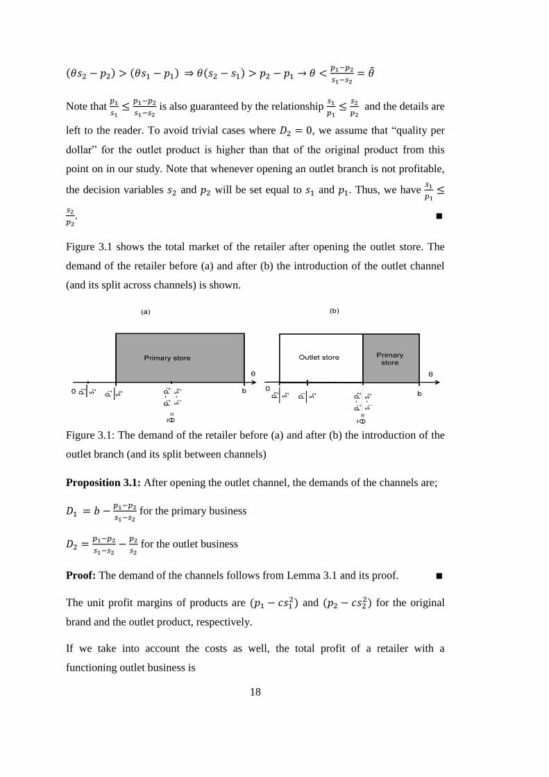
Figure 3.1 shows the total market of the retailer after opening the outlet store. The

demand of the retailer before (a) and after (b) the introduction of the outlet channel

(and its split across channels) is shown.


outlet branch (and its split between channels)

Proposition 3.1: After opening the outlet channel, the demands of the channels are;

for the primary business

for the outlet business

Proof: The demand of the channels follows from Lemma 3.1 and its proof.

The unit profit margins of products are and

for the original

brand and the outlet product, respectively.

If we take into account the costs as well, the total profit of a retailer with a

functioning outlet business is

19

After all, the retailer’s problem can be modeled as,

(Eq.3.1)

(Eq.3.2)

(Eq.3.3)

(Eq.3.4)

(Eq.3.5)

(Eq.3.6)

(Eq.3.7)

Constraint (3.2) and (3.3) ensures that the retailer has the nonnegative demand for

respective the primary and outlet brand after opening the outlet business. Note that

either can be zero. The objective function of the model, (3.1), maximizes the total

profit given the retailer’s original brand position. Constraints (3.4) and (3.5) are

upper limits for decision variables that identify with the outlet business. Constraints

(3.6) and (3.7) are non-negativity conditions for decision variables.

The retailer’s problem is a nonlinear maximization problem with two decision

variables.

Lemma 3.2: The profit function,

is jointly concave in and in the feasible region of and

Proof: The matrix L, Hessian matrix of profit function, is written below:

The leading principal minors are;

20

(of order one)

( of order two)

L is negative definite if where k={1,2} for all leading principal

minors. implies that condition for the leading principal minors is

satisfied. It is concluded that matrix L is negative definite, hence the profit function

of the firm is jointly concave in and .

The optimal solution of the maximization problem is given in Proposition 3.2

Proposition 3.2: The maximizers of the retailer’s problem in (Eq.3.1-3.7) are

and

.

Proof: The first order partial derivatives of the objective function with respect to

and are given below,

Solving

and

simultaneously yields

and

, which is the optimal solution of the unconstrained optimization problem.

The quality level of the new product is equal to one half of quality level of the

original brand and always nonnegative. Thus, satisfies constraints (3.4) and (3.6).

The optimal price of new product is less than one half of price of the original brand,

thus satisfies (3.5). Constraint (3.7) is satisfied since is always

nonnegative with (A.3.2). After plugging and

into constraint (3.2), it becomes

. With (A.3.1) constraint (3.2) is satisfied. Constraint (3.3) is

satisfied by the optimal outlet brand positions. Thus, and

above are also

feasible (and optimal) for the problem in (Eq.3.1)-(Eq.3.7).

21

The optimal outlet price turns out to be less than one half of the primary brand price

though the optimal outlet quality level is exactly equal to one half of primary product

quality. Quality per dollar for the outlet is higher than quality per dollar for the

primary brand. The gap between quality per dollar for the outlet and primary brand

widens as unit cost (c) or the primary brand quality level increases. The outlet quality

increases and the outlet price decreases with the primary brand quality level. Thus,

the retailer elevates its outlet quality as increases, and shifts it to focus towards the

higher consumer segments. As the primary product price increases the optimal outlet

price increases. While quality level of the original brand affect the price and quality

level of the outlet product, price of the original brand only affects the outlet product

price.

Proposition 3.3: Opening the outlet business is preferable for both the retailer and

the consumer. By opening an outlet branch, the retailer’s profit increases by

Proof: Without outlet, demand and profit of the primary business are given by,

(Eq.3.8)

(Eq.3.9)

After rearranging (3.9), it becomes,

(Eq.3.10)

When we plug-in and

values into the retailer’s profit function in (Eq.3.1),

becomes,

(Eq.3.11)

Then,

since and .

Before starting an outlet business, consumer surplus is given by,

(Eq.3.12)

22

When the outlet channel is open, the formulation of the consumer surplus is given

by,

With and

, it becomes ;

(Eq.3.13)

Then

since and .

The consumer surplus and the profit of the retailer before and after the outlet branch

are summarized in Table 3.2.

Table 3.2: Comparing “only primary business“ and “with an outlet branch “ cases on

profit and consumer surplus

Only primary business With an outlet branch

Total profit

Consumer Surplus

Total demand of the retailer increases by

while the demand of the retailer’s

primary business decreases by

after opening the outlet business. Although the

outlet business cannibalizes some of primary business demand; the retailer manages

to increase its overall demand with the addition of the outlet branch.

The market expansion is

and its margin is

or equivalently

.

The cannibalized demand from the primary brand is

and change in the margin is

or equivalently

. The profit margins of products

are equal when

. If

, then the profit margin of the primary

business is always greater than that of the outlet product.

23

As the primary product quality level increases ( , outlet quality level ( increases

and outlet price ( decreases. As a result, demand of the outlet product increases.

As the unit cost coefficient (c) increases, the profit gain increases. As the unit cost

coefficient increases, the optimal outlet price ( decreases but the optimal outlet

quality level ( remains the same. Consequently, the outlet demand increases with

the unit cost coefficient. The retailer achieves market expansion with increase in the

outlet demand. Hence, as unit cost coefficient increases, the extra market increases.

The retailer’s main tradeoff is between market expansion and cannibalization of the

primary store and its profit margin.

When we plug-in and

into , it becomes

. If and remain the

same, as c increases, goes up. In short, the the primary brand demand shrinks

whereas the outlet brand demand becomes larger with the increase in c. The price,

quality level, demand of products in the “only primary business “case and “with an

outlet branch“case are summarized in Table 3.3.

24

Table 3.3: Comparing “only primary business” and “with an outlet branch “cases on

profit, demand, price and quality level of the products

Only primary business With an outlet branch

Profit of the outlet

product

NA

Profit of the primary

product

Total profit

Demand of the primary

product

Demand of the outlet

product

NA

Profit margin of

primary product

Profit margin of outlet

product NA

Total covered market

The primary price

The outlet price NA

The primary quality

level

The outlet quality level NA

We also investigate the retailer’s initial primary brand position strategies. The

retailer can position the primary brand without any consideration of the outlet

business opportunity in the future. In this strategy, the retailer acts myopic. The

myopic retailer positions the primary product and then the outlet product. In long

term planning, the retailer also considers the future outlet product position while

positioning the primary product. For that reason, we refer to that type of retailer as

“non-myopic retailer.” The whole reason behind this is to compare the primary brand

position and profit levels under two strategies.

25

3.1.1 Myopic Retailer

In this part, we investigate the scenario where the retailer positions its primary brand

(i.e., sets and ) only to maximize its primary business profit.

The demand and profit of the retailer are given by (3.8) and (3.9);

(Eq.3.8)

(Eq.3.9)

Lemma 3.3: The profit function of retailer, (Eq.3.9), is jointly concave in and .

Proof: The matrix H, Hessian matrix of profit function, is written below:


(of order one)

(of order two)

H is negative definite if where k={1,2} for all leading principal

minors. The condition for the second leading principal minor is satisfied with

(A.3.1). The profit function of the retailer is jointly concave in and since the

matrix H is negative definite.

The total profit of the retailer can be modeled as follows;

(Eq.3.9)

(Eq.3.14)

(Eq.3.15)

26

The objective function of the model, (3.9), maximizes the profit of primary business.

The constraints (3.14) and (3.15) are non-negativity conditions for decision

variables.

The retailer’s problem is a nonlinear maximization problem with two decision

variables. The optimal solution of the unconstrained maximization problem is given

in Proposition 3.4.

Proposition 3.4: The maximizers of the retailer’s problem in (Eq.3.9, 3.14, 3.15) are

and

.



Solving

and

simultaneously yields two ) pairwise

roots. We find that

and

with objective function value of

. Since

(Eq.3.14) and (Eq.3.15) are also satisfied, the solution above is feasible (and optimal)

for the problem stated.

When

and

, the retailer generates profit of

. If the retailer

started to serve the customer with the outlet store as an additional channel, total

profit would be

.

3.1.2 Non-Myopic Retailer

In this part, we consider the scenario where the retailer takes into account a future

outlet branch opportunity while positioning its primary brand. In other words, we

want to find the primary brand positions that maximize the total profit that includes

the outlet branch that will follow as well. Here, the retailer does not act myopic,

27

makes sequential brand position decisions in case of opening outlet branch is

possible in the future. We refer this type of retailer as a non-myopic retailer.

When we plug-in and

into (3.1), the profit function of the retailer is;

(Eq.3.16)

Lemma 3.4: The profit function of retailer, (3.16), is jointly concave in and .

Proof: The matrix M, Hessian matrix of profit function, is written below:


(of order one)

(of order two)

M is negative definite if where k={1,2} for all leading principal

minors. The condition for the second leading principal minor is satisfied with

(A.3.1). It is concluded that matrix M is negative definite, hence profit function of

the firm is jointly concave in and .

The retailer’s problem is then,

(Eq.3.16)

(Eq.3.14)

(Eq.3.15)

Proposition 3.5: The maximizers of the retailer’s problem in (Eq.3.14, 3.15, 3.16)

are

and

.



28

Solving

and

simultaneously yields two pairwise

roots. We find that

and

with objective function value of

. Since

(Eq.3.14) and (Eq.3.15) are also satisfied, the solution above is feasible (and optimal)

for the problem stated.

When

and

, the retailer generates a profit of

. If the retailer

started to serve the customer with the outlet channel as additional channel, the total

profit would be

.

The findings are summarized in Table 3.4. As a result, primary brand positioning

based on long term planning (non-myopic approach) is preferable for the retailer. If

the retailer acts as opening outlet branch will be possible in the future, then the firm

sets a higher price and a quality level for the primary brand. The profit difference

between two cases exponentially increases with b and decreases with c.

29

Table 3.4: The primary brand position and the total profit in the “myopic” and “non-

myopic” retailer cases

Myopic

Retailer

Non-myopic

Retailer

Price of the

primary brand

Quality level of

primary brand

Total profit of the

retailer (without

outlet)

Total profit of the

retailer (with

outlet)

3.2 The physical outlet decisions of a brick-and-mortar retailer with

inconvenience cost

In Section 3.1, we studied a monopolist firm’s decision about opening an outlet

business without any consideration of an inconvenience cost regarding either

channel. However, that was an idealized case. In real life there exist inconvenience

costs associated with visiting a brick-and-mortar retailer. This may include the actual

activity of visiting the store, time spent on the activity as well as the unavailability

risk of the product. A consumer’s utility decreases with this inconvenience. Note that

outlet malls tend to be located far away from city centers, which translates into a

higher inconvenience cost associated with visiting the outlet store.

Here we investigate the retailer’s outlet branch decisions in the presence of

inconvenience costs for both the primary chain and the outlet stores. We change

utility functions by adding new terms; specifically k>0 for the inconvenience of

visiting the primary brand chain, and m>0 for visiting the outlet chain. We assume

that inconvenience cost of visiting and purchasing from the outlet store is greater

30

than inconvenience cost of visiting and purchasing from the primary store. In short,

(A.3.3)


attribute. A higher type of consumer (i.e.; with a higher taste parameter) is willing to




Consumer of type has the following utility function;

θ θ

We assume that consumers are heterogeneous in their willingness to pay for quality;

i.e., consumers are distributed uniformly on [0, b] according to their types θ, where

We assume that b is high enough to enable a profitable business for the

retailer (i.e.; for nonnegative market share and margin). Again, we assume that the

outlet product is inferior to the primary brand in terms of quality and price. That is,

and .










Table 3.5.

31

Table 3.5: Notation


Quality level of the outlet branch,

Price of the outlet branch,

Quality level of the original brand, , , (given)

Price of the original brand, , , (given)

Parameters


Inconvenience cost of visiting and purchasing from the physical outlet,

Inconvenience cost of visiting and purchasing from the physical store,



Demand of the outlet branch ,

Before opening the outlet channel, the retailer serves the market through the physical

channel of its original brand. A consumer will want to purchase from the primary

physical store if .

denotes the taste parameter of the last

consumer who purchases the product from the primary physical store when there is

only primary physical store in the market. Thus, the demand of the primary business

is given by (

) and the monopolist retailer cannot cover the whole market by

itself.

Lemma 3.5: Outlet branch may have on impact on the retailer’s business if and only

if

; i.e., “quality per dollar” for the outlet product is higher than that of

the original product. The total market of the retailer expands by

,

consumers with in

switch from the primary brand to the

outlet branch.

Proof: Suppose now

. ( In this case

directly holds.)

32

A consumer of type prefers the primary brand to the outlet brand if and only if

.

since

.

if and by assumption

and

Thus, whenever a consumer is willing to buy from the outlet branch, he prefers the

primary brand to the outlet brand and thus never purchases from the outlet.

Therefore, if

, then the outlet branch has zero demand ( and the

primary branch demand is

.

When we have

, we then have

. When

,

the consumer will have a positive utility only if he purchases from the outlet (i.e.,

negative utility from the primary brand).

When

, the consumer will have positive utility from both branches and

prefer the outlet if and only if .

Note that

is also guaranteed by the relationship

and

the details are left to the reader. To avoid trivial cases where , we assume that

“quality per dollar” for the outlet product is higher than that of the original product

from this point on in our study. Thus, we have

.

Figure 3.2 shows the total market share of the retailer after opening the outlet store.

The demand of the retailer before (a) and after (b) the introduction of the outlet

channel (and its split across channels) is shown.

33


outlet branch (and its split between channels) ((p1-p2+k-m)/(s1-s2) b)

Proposition 3.6: After opening the outlet channel, the demand for each channel is;

for the primary business

for the outlet business

Proof: The demand of the channels follows from Lemma 3.5 and its proof.

The retailer’s problem can be written as follows:

(Eq.3.17)

s.to

(Eq.3.18)

(Eq.3.19)

(Eq.3.4)

(Eq.3.5)

(Eq.3.6)

(Eq.3.7)

Constraint (3.18) and (3.19) ensures that the retailer has the nonnegative demand for

respective the primary and outlet brand after opening the outlet business. Note that

34

either can be zero. The objective function of the model, (3.17), maximizes the total

profit given the retailer’s original brand position. Constraints (3.4) and (3.5) are

upper limits for decision variables that identify with the outlet business. Constraints

(3.6) and (3.7) are non-negativity conditions for decision variables.

Proposition 3.7: The profit function of the retailer, (Eq.3.17), is not jointly concave

in and . Nor is it convex.

Proof: The matrix S, Hessian matrix of profit function, is written below:


(of order one)

( of

order two)

Before evaluation, we want to summarize positive and negative definiteness of

matrix S.

S is negative definite if where k= {1, 2} for all leading

principal minors. Therefore, the profit function is jointly concave in and

.

S is positive definite if where k= {1, 2} for all leading principal

minors. Therefore, the profit function is jointly convex in and .

The principal minors depend on the decision variables ( and and change signs

in the feasible region. We show that the concavity or convexity conditions are not

satisfied by a counter example. The parameters are listed in Table 3.6.

35

Table 3.6: The parameters of the example

Parameter Value

6

6

0.9

0.1

The leading principal minors are calculated with these parameter for

and . Table 3.7 shows leading principal minors for some (

values that satisfy both (A.3.3) and

.

Table 3.7: The leading principal minors for some (s2, p2) values

5 1 -2.4 14.085

5 2 -2.4 6.961

5 3 -2.4 2.142

5 4 -2.4 -0.372

4 1 -1.5 1.807

4 2 -1.5 0.635

4 3 -1.5 0.026

3 1 -1.333 0.454

3 2 -1.333 0.029

2 1 -1.5 0.006

Here, the first leading principal minor is always negative. However, the second

leading principal minor is sometimes negative and sometimes positive. The joint

concavity requires and . However, there is case where the second

leading principal minor is negative. Thus, in our feasible range, the profit function

may not be jointly concave in and . The joint convexity requires .Thus,

we conclude that the profit function is not jointly convex in and .

36

Since the profit function is not jointly concave or convex in and , we analyze its

behavior with respect to and individually next.

When the quality level of the outlet brand is given, the total profit becomes a

function of . The profit function of the retailer with respect to non-negative

demand of outlet channel is written below,

If the profit function is rearranged based on , it becomes ;

(Eq.3.20)

Proposition 3.8: For a given , the retailer’s profit function (Eq.3.20) is concave in

in the feasible region of

Proof: The second order derivative with respect to is given below,

The implies that the SOC of the profit function is negative.

We can find the maximizer (for a given using the FOC of the profit function

as follows;

Step 0: Find which satisfies

.

Note that

and

Step 1: If

, then

and .

37

Step 2: If

, then set

. When

,

the demand of outlet equals to zero and the profit function equals to

.

When is given, the total profit becomes a function of as a decision variable as

follows:

The profit function of the retailer based on is written below,

(Eq.3.21)

Proposition 3.9: For a given , the retailer’s profit function (Eq.3.21) is concave in

in the feasible region of

Proof: The second order derivative with respect to is given below,

It is known that and . Hence, the first term of the SOC of the

profit function with respect to is negative. As a result, the SOC of the profit

function is negative.

We can find the maximizer (for a given using the FOC of the profit function

as follows;

Step 0: There are four roots ( to satisfy

.

Note that

Step 1: If

, then

and

.

38

Step 2: If there is no which is in that interval, put differently,

, then

set

When

, the demand of outlet channel equals to zero

and the profit function equals to

.

3.3 Numerical analysis on the outlet decisions with inconvenience costs

We studied the outlet business decisions in the presence of inconvenience costs.

However, the total profit of the retailer, (Eq.3.17) is neither jointly concave nor

jointly convex in and . For that reason, in this section, we aim to analyze the

effect of inconvenience cost on the optimal quality level and price of the new

product, demands of the primary store and outlet channel, market size and profit of

the retailer.

In our numerical experiments, we used 40 for b, 0.1 for c, tested for k in [0, 3] with

the amount of increment by 0.01 and m in [k, 3] with the amount of increment by

0.01. We set 0.01 as the lower bound of both and and limited our experiments

to the cases where and .

We create two groups of trials each of which contains four combinations of and

All trials are presented in Table 3.8

Table 3.8: The first and second group of trials

The first group of trials The second group of trials

Trial 1 Trial 2 Trial 3 Trial 4 Trial 5 Trial 6 Trial 7 Trial 8

8 8 8 8 8 6 4 2

8 10 12 14 8 8 8 8

We use 0.01 as the amount of increment for the feasible interval of . In this

respect, different increment is used/calculated for the to equalize the number of

and values; i.e., 0.0064 for trial 1, 0.009 for trial 2, 0.0117 for trial 3, 0.0144 for

trial 4, 0.0086 for trial 6, 0.0132 for trial 7, 0.0279 for trial 8. Thus, in each trial, we

form the ( ) matrix for the feasible interval of and . In each trial, the

39

optimal outlet quality level and price is chosen from this matrix in order to maximize

the retailer’s total profit for a set of b, c, m and k.

We find that for a given k, as m increases,

and profit of the retailer

decreases but increases. Thus, demand and profit margin of the outlet decrease.

Here, decreases because the retailer compensates for the high outlet

inconvenience. In this environment, will be low because the retailer cannot afford

a high product cost any more. When m is high, the retailer has to position the outlet

business as a lower quality, lower price alternative. As a result, the total outlet

demand decreases whereas the primary brand demand increases. For all trials, for a

given k, as m increases, profit margin of the outlet decreases. Figure 3.3 and 3.4

show versus m and

versus m plots for trial 2 when k=0.5, respectively. See

Appendix A for versus m,

versus m, retailer’s profit versus m, total market

versus m and

versus m plots for trial 2 when k=0.5 and related data.

Figure 3.3: s2* versus m plot for trial 2 when k=0.5

Figure 3.4: p2* versus m plot for trial 2 when k=0.5

0

1

2

3

4

5

0.5 0.7 0.9 1.1 1.3 1.5 1.7 1.9 2.1 2.3 2.5 2.7 2.9

ou

tle

t q

ual

ity

(s2

)

m

0 0.5

1 1.5

2 2.5

3 3.5

4 4.5

5

0.5 0.7 0.9 1.1 1.3 1.5 1.7 1.9 2.1 2.3 2.5 2.7 2.9

ou

tle

t p

rice

(p

2)

m

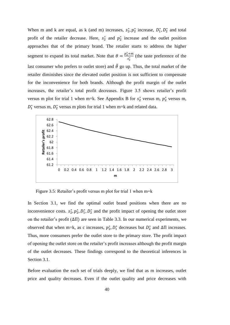
40

When m and k are equal, as k (and m) increases,

increase,

and total

profit of the retailer decrease. Here, and

increase and the outlet position

approaches that of the primary brand. The retailer starts to address the higher

segment to expand its total market. Note that

(the taste preference of the

last consumer who prefers to outlet store) and go up. Thus, the total market of the

retailer diminishes since the elevated outlet position is not sufficient to compensate

for the inconvenience for both brands. Although the profit margin of the outlet

increases, the retailer’s total profit decreases. Figure 3.5 shows retailer’s profit

versus m plot for trial 1 when m=k. See Appendix B for versus m,

versus m,

versus m,

versus m plots for trial 1 when m=k and related data.

Figure 3.5: Retailer’s profit versus m plot for trial 1 when m=k

In Section 3.1, we find the optimal outlet brand positions when there are no

inconvenience costs.

and the profit impact of opening the outlet store

on the retailer’s profit ( are seen in Table 3.3. In our numerical experiments, we

observed that when m=k, as c increases,

decreases but and increases.

Thus, more consumers prefer the outlet store to the primary store. The profit impact

of opening the outlet store on the retailer’s profit increases although the profit margin

of the outlet decreases. These findings correspond to the theoretical inferences in

Section 3.1.

Before evaluation the each set of trials deeply, we find that as m increases, outlet

price and quality decreases. Even if the outlet quality and price decreases with

61.2

61.4

61.6

61.8

62

62.2

62.4

62.6

62.8

0 0.2 0.4 0.6 0.8 1 1.2 1.4 1.6 1.8 2 2.2 2.4 2.6 2.8 3

Re

taile

r's

pro

fit

m

41

increase with m, the decrease in the demand of the outlet cannot be prevented. Thus,

the outlet impact on the market and retailer’s profit decreases.

After inferences with initial observations for all trials, we want to evaluate the each

set of trials deeply. Firstly, we focus on the first group of trial. To make inferences,

we plot versus m,

versus m, versus m,

versus m,

versus m,

total market versus m and retailer’s profit versus m graphs for a given k.

In the first group of trials, trial 1 has the lowest value when all trials have the

same value. Thus, when there is only primary brand in the market, trial 1 has the

largest market potential. It can be also that trial 1 is the most competitive one in the

first set of trials.

We observe that trial 1 produces the lowest value. As the primary brand gets more

competitive in terms of price, the outlet price level tends to be lower as well. Figure

3.6 show for the first group of trials when k=0.3.

Figure 3.6: p2* for the first group of trials when k=0.3

We see that trial 1 has the highest value after opening the outlet store. Trial 1

sustains the largest market potential with the outlet store as well. After opening the

outlet store, the rank of will not be changed, but of course,

values will be

decreased. See Figure C.1 for of the first group of trials when k=0.3 in Appendix

C.

0

1

2

3

4

5

6

7

0.3 0.5 0.7 0.9 1.1 1.3 1.5 1.7 1.9 2.1 2.3 2.5 2.7 2.9 m

Optimal p2 for trial 1




42

We see that value for the first group of trials is almost identical to each other.

Figure 3.7 shows for the first group of trials when k=0.3.

Figure 3.7: s2* for the first group of trials when k=0.3

We see that value for the first group of trials is close to each other. It is the most

interesting observation. Trial 1 is expected to have the highest value since it has

the lowest value with about the same

values across the first set of trials. Thus,

the resulting and

values are rarely impacted by the price competitiveness

of the primary brand. Figure 3.8 shows for the first group of trials when k=0.3.

Figure 3.8: D2* for the first group of trials when k=0.3

0

0.5

1

1.5

2

2.5

3

3.5

4

4.5

5

0.3 0.5 0.7 0.9 1.1 1.3 1.5 1.7 1.9 2.1 2.3 2.5 2.7 2.9

Ou

tle

t q

ual

ity

(s2

)

m

Optimal s2 for trial 1




0

0.05

0.1

0.15

0.2

0.25

0.3

0.35

0.4

0.3 0.5 0.7 0.9 1.1 1.3 1.5 1.7 1.9 2.1 2.3 2.5 2.7 2.9

De

man

d o

f th

e o

utl

et

bra

nd

m

Optimal D2 for trial 1




43

We see that trial 4 produces the highest profit. values are close across the first set

of trials whereas trial 1 has the highest value and trial 4 has the largest profit

margin of products. Thus, profit margins of the primary and outlet businesses are

more significant than market share in determining the profit of the retailer.

Later, we evaluate the second group of trials. Again, we plot versus m,

versus

m, versus m,

versus m,

versus m, total market versus m and

retailer’s profit versus m graphs for a given k.

In the second group of trials, trial 5 has the highest value when all trials have the

same value. When there is only the primary brand in the market, trial 5 has the

largest market potential. It can also be that trial 5 is the most competitive one in the

second group of trials.

We observe that trial 5 produces the highest and lowest

. As the primary brand

gets more competitive in terms of quality, the outlet quality increases and the outlet

price level decreases. Thus, trial 5 has the lowest profit margin of the outlet business.

Trial 5 sustains a viable outlet business in high inconvenience costs as well. Figure

3.9 and 3.10 show versus m and

versus m plot for the second group of trials

when k=0.3.

Figure 3.9: s2* for the second group of trials when k=0.3

0

0.5

1

1.5

2

2.5

3

3.5

4

4.5

0.3 0.5 0.7 0.9 1.1 1.3 1.5 1.7 1.9 2.1 2.3 2.5 2.7 2.9

Ou

tle

t q

ual

ity

(s2

)

m





44

Figure 3.10: p2* for the second group of trials when k=0.3

We see that trial 5 produces the highest value after opening the outlet store. We

observe that trial 5 produces the largest naturally since it produces the highest

and the lowest value. Thus, trial 5 has the largest total market. Figure 3.11 shows

versus m plot for the second group of trials when k=0.3. See Figure D.1, D.2 for

the second group of trials when k=0.3 in terms of and retailer’s total market in

Appendix D.

Figure 3.11: D2* for the second group of trials when k=0.3

0 0.5

1 1.5

2 2.5

3 3.5

4 4.5

5 5.5

6 6.5

7

0.3 0.5 0.7 0.9 1.1 1.3 1.5 1.7 1.9 2.1 2.3 2.5 2.7 2.9

Ou

tle

t p

rice

(p

2)

m





0

0.05

0.1

0.15

0.2

0.25

0.3

0.35

0.4

0.3 0.5 0.7 0.9 1.1 1.3 1.5 1.7 1.9 2.1 2.3 2.5 2.7 2.9

De

man

d o

f th

e o

utl

et

bra

nd

(D

2)

m





45

We see that trial 8 produces the highest profit. Trial 5 has the largest and

and

trial 8 has the highest profit margin of product. We find that the profit margins of the

primary and outlet business are more significant than market share to determine the

profit of the retailer as observed in the first set of trials.

It is observed different from the first group of the trials that as the primary brand gets

more competitive in terms of quality level, it gets easier to position and justify an

outlet brand. Outlet becomes more competitive both in price and quality; as opposed

to just price that we observed in the first group of trials.

In this chapter, we characterize the outlet brand positions and evaluate the profit

impact of the outlet store. The analysis is conducted in two different settings. In the

first setting, inconvenience costs are neglected. In Section 3.1, we find that opening

the outlet business is preferable both the retailer and the consumer. The retailer

manages to expand its total market although the outlet business cannibalizes the

demand of the primary brand. Quality per dollar for the outlet is higher than quality

per dollar for the primary brand. The gap between quality per dollar for the outlet

and primary brand widens as unit cost (c) or the primary brand quality level

increases. The outlet quality increases and the outlet price decreases with the primary

brand quality level. Thus, the retailer elevates its outlet quality as primary brand

quality level increases, and shifts it to focus towards the higher consumer segments.

Outlet quality increases with the primary brand quality and does not depend on cost

and prices at all. As the unit cost (c) increases, the profit gain and the generated

market with the outlet increase. The retailer’s main tradeoff is between market

expansion and cannibalization of the primary store and its profit margin.

According to primary brand strategies, retailers are classified in two groups: myopic

and non-myopic retailer. We find that non-myopic approach is preferable for the

retailer in terms of profit since it enables firm to set higher price. Also, the consumer

is offered a higher quality level of the primary brand when the retailer is non-

myopic.

46

In the second part of the chapter, we take into account inconvenience costs

associated with visiting a brick-and-mortar retailer. An extensive numerical study is

conducted to evaluate the changes in the outlet product position, demand of primary

and outlet business and total profit of the retailer in the presence of inconvenience

cost since the analytical approach to find the optimal outlet product position is not

suitable.

In Section 3.3, we create two groups of trials each and parameters set for numerical

study. The two groups are different from each other in terms of competitiveness in

price and quality level. As the primary brand gets more competitive in terms of

quality and price, the outlet price level tends to be lower. The price competitiveness

of the primary brand does not impact the quality level and demand of the outlet

brand. However, as the primary brand gets more competitive in terms of quality, it

produces the larger market size for the outlet brand and the outlet quality level tends

to be higher. Independent of competitiveness in price and quality level, we find that

the profit margins of the primary and outlet business are more significant than

market share in determining the profit of the retailer. In the second set of trials, trial

5 sustains a viable outlet business longest. We find that as the primary brand gets

more competitive in terms of quality level, its outlet business becomes more robust

(viable) than others.

47

CHAPTER 4

ONLINE CHANNEL DECISION FOR A BRICK-AND-MORTAR

RETAILER

In this chapter, we are interested in a monopolist retailer’s online channel decision

when the original brand is already available in the physical store.

In real life visiting the physical stores is associated with some inconvenience. The

inconvenience cost may comprise physically going to the store; time spent on the

activity as well as the stock-out risk that may send the consumer home empty-

handed. Consumers are freed from the physical inconvenience cost when they

purchase online. However, buying from the online channel does not offer immediate

gratification; the customer now needs to wait for a pre-specified time to receive his

product and now faces new risks associated with product properties such as the fit,

color, and size. Hereby, an additional dimension on which consumers differ emerges;

sensitivity to online services and promised delivery time.

Online service quality may involve all customer services provided by the online

store, the convenience of return process, and promised delivery time windows as

well as shipping charges. In the rest of this thesis, we interchangeably refer to this

dimension as promised delivery time. Here, we use t to refer to this dimension in a

reverse way; that is, the lower t is, the higher the online service quality. Note that t

here represents all the online services offered to the customer including but not

limited to the promised delivery time.

In this chapter, the retailer’s major decision is to determine the online service quality

(the promised delivery time, t) to maximize the retailer’s total profit for a given set

of original brand positions and inconvenience cost of going to store (k).

48

We assume that the promised delivery time can be set in a feasible time interval

where and all practical feasible delivery times are in this interval. In practice,

online service and delivery options are limited by external factors. For example

overnight delivery is the faster option available to most retailers.

In this chapter, a consumer wants to maximize the following utility function:

θ θ




The utility of the consumer who uses the online channel decreases as s/he waits, the

utility of the consumer who purchases from the offline store decreases due to the

inconvenience regarding the physical channel.

We assume that consumers differ in willingness to pay for quality and in sensitivity

to online services and promised delivery time while purchasing at the online channel;

i.e.; consumer types are distributed uniformly on [0, b] according to their types d and

, where b>0. We assume that b is high enough to enable a profitable business for

the retailer (i.e.; for nonnegative market share and margin). In this chapter, we

assume that

(A.4.1) and

(A.4.2) to ensure nonnegative

market share.


attribute. A higher type of consumer (i.e.; with a higher taste parameter) is willing to




A consumer of type d has a diminished utility by dt when he has to wait for a period t

before receiving the product. As d increases, the consumer becomes more time

49

sensitive (i.e., impatient), and thus he starts preferring the physical store to the online

store since the physical store offers instant gratification.







Table 4.1.

Table 4.1: Notation


Quality level of the original brand, (given)

Price of the original brand, (given)

The online service quality set for the online channel, ]

Parameters




Sensitivity index to online services and promised delivery time of consumer,

Online channel cost coefficient,


Demand of the outlet branch,

Proposition 4.1: For a given positive promised delivery time at the online channel

(t>0),

i. Consumers who purchase from the physical store decrease from all and

all to all and where

50

ii. Consumers with and switch from the physical channel to the

online channel. The retailer also expands its market by

through the online

channel.

iii. The demand characterization of the channels is

Proof: A consumer will want to purchase from the online store if

and from the physical store if He will choose the online store if

.

So for any consumer type with so that , if

, then the

consumer will prefer the online to offline store.

If but , then consumer will purchase from the online

store if (

.

Then, will consist of consumers that and . Thus,

.

The demand of the online store will become;

.

Figure 4.1 shows overall demand of the retailer after opening the online channel. The

triangular area is the extra demand that the retailer generates through the online

channel.

51

Figure 4.1: Total demand after the introduction of the online channel (and its split

among channels)

Corollary 4.1: The retailer’s total market increases as t decreases.

Proof: According to Proposition 4.1, the total market of retailer expands by

. As t

decreases, market expansion increases.

Based on Corollary 4.1, if the retailer did not have any cost for online services, he

would want to set t as low as possible. However, this is not a realistic case.

Generally, serving through the online channel creates additional costs for the retailer

including call centre management, courier services, returns management and etc. The

retailer has to incur a certain cost to make the delivery of the product in the promised

time window t and provide online services. For that reason, there arises the cost

versus the market expansion tradeoff associated with setting the delivery time. We

assume that the firm incurs online channel cost

as the unit cost of serving an

online customer where z is the online channel cost coefficient. As online services

improve; i.e., as t decreases, the cost incurred to deliver it increases exponentially.

We assume that z (online channel cost coefficient) is high enough to discourage the

firm to set t=0. (or serve the market perfectly.) In this chapter, we assume that

(A.4.3).

The unit profit margins of the primary and online channel are ( and

, respectively.

52

If we take into account the costs as well, the total profit of the retailer can be

summarized as follows:

)


(Eq.4.1)

s.to (Eq.4.2)

The objective function of the model, (4.1), maximizes the total profit when the

retailer serves the customers through both channels with its original brand.

The retailer’s problem is a nonlinear maximization problem.

Lemma 4.1: The profit function,

) is concave in the promised delivery time t when

.

Proof: The second order derivative of the objective function with respect to t is

given below,

.

It is clear that

is always positive since . Hence, if

, then

. This expression is a second-degree polynomial

in t. The discriminant of this expression is given below,

(A.4.1) and (A.3.2) ensure that the discriminant is always positive. Then the SOC of

the profit function becomes negative when

.

Thus, the SOC is always negative in feasible region .

53

The optimal solution of the maximization problem is given in Proposition 4.2.

Proposition 4.2: While opening an online channel, the retailer sets min

where

.

i.If , then .

If , then the retailer finds it profitable to open the online

channel.

Otherwise, the profit impact of the online channel on the retailer’s

profit ( is always negative.

ii.If , and profit impact of the online channel on the

retailer’s profit ( always nonnegative.

where

and

.

Proof: The first order derivative with respect to t is given below,

Solving

yields

. If , then is the

maximizer of the total profit function.

The change (i.e., decrease) in the profit of the retailer with respect to drop in the

profit of primary store is

(Eq.4.3)

The increase in the profit of the retailer with respect to gain in the profit of the online

channel is;

(Eq.4.4)

After combining (4.3), (4.4), the change in total profit is;

(Eq.4.5)

54

The retailer will find it profitable to open then online channel if and only if .

When , then the net change in the total profit of the retailer is;

(Eq.4.6)

if and only if .

When , after plugging into (4.5), the net change in the total profit is;

(Eq.4.7)

When , the net change in the total profit is ;

(Eq.4.8)

Note that if and only if

.

Since we know that and , we must have

as

well.

Whenever the optimal promised delivery time is or , since they are constant, the

relationships below weakly hold. Here, we analyze change in with respect to the

parameters in our model.

Corollary 4.2: As increases, increases. If k or increases, decreases.

Proof: The first order derivative with respect to are given below,

55

implies that . Then,

which makes the whole expression negative.

implies that . The FOC of with respect

to becomes positive if the highest value of which is is plugged

into denominator of

.

Intuitively, as k increases, utility derived from physical channel decreases. Thus,

consumers who suffer from low utility value derived in physical store can begin to

use the online channel. The retailer wants to capture these consumers by shortening

the delivery time.

The retailer’s main tradeoff is between market expansion and cannibalization of the

physical channel demand and online margin loss. As k or increases, market

expansion starts to dominate, hence decreases. As z or c increases, loss in the

profit margin dominates, hence increases.

Corollary 4.3: If , then . The net change in the

retailer’s profit ( is increasing in k and , and decreasing in c, , z and b

where

Proof: The first order derivative with respect to are given below,

56

can be written . If the lowest value of

which is is plugged into the denominator of

, then the FOC of profit

with respect to becomes positive.

implies that . If the highest value of

which is is plugged into the denominator of

, then the FOC of

profit with respect to becomes negative.

Intuitively, the better online service quality is costly. The common parameters

influence and in opposite way. That is, as k or increases, the online

channel becomes more aggressive but increases. As increases, the

online channel gets less effective but decreases. In the high online service cost

environment, the retailer may lead to lengthen the optimal promised delivery time.

Thus, decreases. As the price of the primary brand increases and quality level of

the primary brand decreases, increases.

Table 4.2 summarizes the demand and profit measures of the “physical chain only”

scenario with the “both online and physical “ case.

57

Table 4.2: The comparisons between “only physical chain” and “both online and

physical chain”

only physical chain both online and physical chain

Demand of physical

store

)b

Demand of online store NA

Profit margin of

physical store

Profit margin of online

store NA

Profit of physical store

)

)

Profit of online store NA

Total profit

)

Total covered market

The optimal online service quality ( , (i.e.; the retailer’s profit change with

opening the online channel) can be investigated together with respect to the online

cost parameter of the market environment, z.

Figure 4.2 and 4.3 summarize the evolution of the profit impact of the online channel

and the optimal promised delivery time with respect to z for Order 1 and 2,

respectively. Depending on the problem parameters, both orders are feasible. See

Appendix E for Lemma 4.2 and its proof.

58


cost (Order 1)


cost (Order 2)

In this chapter, we find that opening the online channel expands the retailer’s market

although it cannibalizes the other channel. When physically inconvenience cost of

going to store is high enough, utility derived from physical channel decreases and

consequently consumers who suffer from low utility value derived in physical store

can begin to use the online channel. Thus, market expansion occurs through the

online channel. In fact, market expansion increases as the physical channel quality

decreases.

When online service cost is low enough, the online channel represents big

opportunity for the retailer. As the price of the primary brand increases and quality

level of the primary brand decreases, the profit impact of the online channel

increases. Otherwise, generated market is small and the profit impact of the online

channel can be positive or negative. When providing online services is costly, the

retailer will keep the online service level as low as possible and decreases.

59

CHAPTER 5

ONLINE CHANNEL DECISION FOR A BRICK-AND-MORTAR

RETAILER WITH AN OUTLET BRANCH

In this chapter, we are interested in a monopolist retailer’s online channel decision

for the primary brand while the retailer is already managing its original and outlet

brand through the respective physical channels. We assume that both business

branches are viable; that is, they have positive demand and profit margin. That is,

(A.3.2),

(A.5.1) and

(A.5.2),

. (A.5.3).

The retailer’s main decision is to determine the service quality to be offered at the

online channel of the original brand in order to maximize the retailer’s profit for a

given set of original and outlet product positions and

inconvenience cost of going to the stores (m and k). The parameters, decision

variables and notations used in this chapter are presented in Table 5.1.

We assume that inconvenience cost of visiting and purchasing from the outlet stores

is greater than inconvenience cost of associated with the physical brand chain since

outlet malls are located far away from city centers. In short, (A.3.3).

Similar to the previous chapter, the effectiveness of the online channel as an

additional sales channel depends on the committed online service level (e.g.,

promised delivery time, t). We assume that consumers differ in sensitivity to the

online service and promised delivery time while purchasing online and in

willingness-to-pay for quality; i.e., consumer types are distributed uniformly on [0,

b] according to their types d and , where b>0. We assume that b is high enough to

60

enable a profitable business for the retailer (i.e., for nonnegative market share and

margin).

When the promised delivery time is taken into consideration, we assume that t can be

set in a feasible time interval , where and all practical delivery times are

in this interval since online service and delivery options are limited by external

factors.

We assume that the firm incurs online channel cost

as the unit cost of serving an

online customer where z is the online channel cost coefficient. In this chapter, again,

we assume that

(A.4.2) to ensure nonnegative market share for a

potential online channel.

In our model, a consumer has the following utility function,




The utility of the consumer who uses the online channel decreases as he waits, the

utility of the consumer who purchases from the offline store decreases due to the

inconvenience regarding the physical channel.

61

Table 5.1: Notation

Decision Variable (s)



Quality level of the outlet branch, (given)

Price of the outlet branch, (given)

The online service quality set for the online channel,

Parameters









Demand of the primary online channel,

Lemma 5.1: Let denote the quality taste parameter of the last consumer who

purchases the product from the outlet store when there is only outlet store in the

market; denote the quality taste parameter of the last consumer who purchases the

product from the online store when there is only online store in the market; denote

the quality taste parameter of consumer that would be indifferent between purchasing

the product from the online channel and the outlet store. (

,

and

)

The orders of and are the only feasible ones among all

possible rankings of and .

Proof: The number of all possible orders is six. These are ,

, , , and .

62

i. If evaluating , simplifies into

. This

expression is consistent with in the first rank.

ii. If evaluating , simplifies into

. This

expression is in contradiction with except for the case .

iii. If evaluating , simplifies into

. This


iv. If evaluating , simplifies into

This


v. If evaluating , simplifies into

. This


vi. If evaluating , simplifies into

. This

expression is consistent with in the sixth rank.

Note that

is always greater than since

always

holds by (A.5.1). Finally,

always holds.

Proposition 5.1: For a given positive promised delivery time (t) at the online

channel, the demand of primary store, outlet store and online channel are given by;

i. For Case 1, i.e., when

for the primary physical store (Eq.5.1)

for the outlet store (Eq.5.2)

for the online store of the primary brand (Eq.5.3)

ii.For Case 2, i.e., when

for the primary physical store (Eq.5.4)

for the outlet store (Eq.5.5)

63

for the online store of the primary brand

(Eq.5.6)

Proof: A consumer will want to purchase from the online store if

and from the physical store for the primary brand if He will

choose the online store if .


, then the

consumer will prefer the online channel to the physical store for the primary brand.

Thus, consumers with and switch from the physical channel to

the online channel. Then,

.

A consumer will want to purchase from the online store if and

from the outlet store if He will choose the online store if

.


,

then the consumer will prefer the online channel to the outlet store.

Thus, consumer with

switch from the outlet store to the online

channel. Then,

The online channel will consist consumer with and , capture

consumer with

from the outlet store. Then,

.

We leave the demand derivation for Case 2 to the reader.

64

Corollary 5.1:

i. Under Case 1 of Proposition 5.1, opening the online channel does not change the

total market of the retailer.

ii. Under Case 2 of Proposition 5.1, opening the online channel expands the total

market of the retailer.

Proof: Left to the reader.

Under Case 1 of Proposition 5.1, the online channel only cannibalizes the primary

and outlet store and cannot create additional demand. Figure 5.1 shows the change in

the retailer’s demand with the online channel under Case 1.


online channel (and its split among channels) under Case 1

Under Case 2 of Proposition 5.1, although the online channel cannibalizes the

primary and outlet store, it creates additional demand. Figure 5.2 shows the change

in the retailer’s demand with the online channel under Case 2.

65


online channel (and its split among channels) under Case 2

5.1 The optimal online service under Case 1

The unit profit margins of the primary and outlet store and online channel are

( ,

and

, respectively.

We assume that z (online channel cost coefficient) is high enough to discourage the

retailer to target the lowest t possible (or serve the market perfectly through the

online channel). In this part of chapter, we assume that

(A.5.4).

If we take into account the costs as well, the total profit of the retailer can be

summarized as follows:


(Eq.5.7)

s.to

The objective function of the model, (5.7), maximizes the total profit of the retailer if

the retailer serves the online consumers with its original brand when the primary and

outlet physical channels are available; i.e., when and are given.

The retailer’s problem is a nonlinear maximization problem.

66

Lemma 5.2: The profit function

is concave in delivery time t when .

Proof: The SOC of the total profit function is given below.

It is clear that

is always positive since delivery time is always positive. The

remaining expression is

(Eq.5.8)

i. If

, the total profit function is concave in t since (5.8)

and also the SOC of the profit function is always negative.

ii.If

, then the SOC of the profit function becomes

negative when

.

The SOC is always negative in feasible region with (A.5.4).


Proposition 5.2: Let denote the profit impact of the online channel on the

retailer’s profit under Case 1.

i. When

, the retailer will set the optimal delivery time

as high as possible (i.e., ) and never find it profitable to open the online channel.

ii. When

, the retailer sets min

where

.

If

, then ,

67

If

, then the retailer

finds it profitable to open the online channel.

Otherwise, .

If , then and always holds.

Proof: The first order derivative of the objective function with respect to t is given

below,

(Eq.5.9)

Solving

yields

. If , then is

the maximizer of the total profit function.

The change (i.e., decrease) in the profit of the retailer in each respective channel are;

(Eq.5.10)

(Eq.5.11)


channel is;

(Eq.5.12)

After combining (5.10), (5.11), (5.12), the change in total profit is;

(Eq.5.13)

The retailer will find it profitable to open then online channel if and only if

.

i. If (5.9) is evaluated, it is positive for all if

. To

generate maximum profit, the retailer sets the optimal delivery time to the maximum

feasible level; i.e.; .

68

(5.13) becomes

(Eq.5.14)

(5.14) is always negative when

.

ii. When , then the net change in the total profit of the retailer is the same as

(5.14). if and only if .

When , after plugging into (5.13), the net change in the total profit is

(Eq.5.15)

is always positive when


(Eq.5.16)


.


as

well.

is increasing with margin difference (

and k.

As quality level difference ( , z, m or b increases, the net gain in the profit

decreases.

69

Whenever the optimal promised delivery time is or , since they are constant, the

relationships below weakly hold. Here, we analyze change in under Case 1with

respect to the parameters in our model.

Corollary 5.2: If

, then

. As z, b, m, , c or increases, increases. If k, or increases,

decreases.

Proof: The first order derivative with respect to z, k, b, m, , , c, , are given

below,

implies that

. Hence, the numerator of

is negative.

implies that

.Hence, the numerator of

is negative and

is positive.

70

implies that

Hence, the numerator of

is positive.

implies that the maximum value of

( is With this the numerator of

is negative.

We investigate increase (or decrease) in the and with respect to common

parameters which are and . As increases, decreases

and increases. Also, as increases, increases and decreases. In

short, while increases (decreases), decreases (increases) with the increase in the

common parameters.

The magnitude of can be interpreted as the outlet market effectiveness

(competitiveness). While the outlet market effectiveness (competitiveness) increases,

decreases. Case 1 may only help the retailer if the online channel attracts more

outlet customers than it cannibalizes from the primary store. Thus, as increases, it

can be more competitive in the online service as well.

5.2 The optimal online service under Case 2

Here, we assume that z (online channel cost coefficient) is high enough to discourage

the retailer to target the lowest t possible (or serve the market perfectly through the

online channel). In this part of chapter, we assume that

where

(A.5.5).

Note that

implies that .

The retailer’s problem can be modeled as,

71

(Eq.5.17)

s.to

The objective function of the model, (5.17), maximizes the total profit of the retailer

if the retailer serves the online consumers with its original brand when the primary

and outlet physical channels are available; i.e., when and are given.

The retailer maximizes its total profit. The nonlinear maximization problem that it

has can be characterized as below.

Lemma 5.3: The profit function

is concave in delivery time t when .

Proof: The SOC of the total profit function is given below.

where

In order to understand the total profit function is concave, the conditions are listed

below.

i. If

(

the condition of

always holds.), then the SOC of the

profit function becomes negative when

. Thus, the SOC is always

negative in feasible region with (A.5.5).

ii. If

,

the total profit function is concave in t.

72


Proposition 5.3: Define .

Let denote the profit impact of the online channel on the retailer’s profit under

Case 2.

i. If

,

then the retailer will set the optimal delivery time as high as possible (i.e., and

never find it profitable to open the online channel.

ii. If

holds (which is directly guaranteed when

), then the

retailer sets min(max(

where

If , then ,

If ,

Otherwise, .

If , then and always holds

where

and

.

Proof: The first order derivative of the objective function with respect to t is given

below,

(Eq.5.18)

73

. is obtained by solving

If , then is the maximizer of the total profit function.

The change (i.e., decrease) in the profit of the retailer in each respective channel are;

(Eq.5.19)

(Eq.5.20)


channel is;

(Eq.5.21)

After combining (5.19), (5.20), (5.21), the change in total profit is;

(Eq.5.22)

The retailer will find it profitable to open then online channel if and only if

.

i. If (5.18) is evaluated, it is positive for all

if

.

To generate maximum profit, the retailer sets the optimal delivery time to the

maximum feasible level; i.e.; .

(5.22) becomes;

(Eq.5.23)

(5.23) is always negative when

74

.

ii. When then the net change in the total profit of the retailer is the same as

(5.23). if and only if .

When , after plugged in to (5.22), the net change in the total profit is

(Eq.5.24)

(5.24) is always positive when

.


(Eq.5.25)


.


as

well.

See Appendix F (Proposition 5.4 and its proof) and G (Proposition 5.5 and its proof)

for profit impact of online channel on the retailer’s profit under Case 1 and 2 with

respect to online service cost, respectively.

As detailed above, two cases may arise depending on the problem parameters in this

setting: Case 1 and Case 2. The retailer manages to expand its market under Case 2

but not under Case 1. The online channel cannibalizes the physical primary and

75

outlet store in both cases. We find that markets that correspond to Case 2 are more

likely to produce a profit increase for the retailer through the online channel. In fact,

the profit margin threshold for positive profit impact under Case 2 is less strict than

that under Case 1.

The online channel profitability is determined by two factors: the difference of profit

margin between the original and outlet product and the online service cost. If the

profit margin of the primary brand is lower than that of the outlet brand, opening the

online channel under two cases is not profitable for the retailer at all. The retailer sets

the optimal promised delivery time as high as possible to avoid any profit loss.

Otherwise, when the online service cost (z) is low enough, the profit impact of the

online channel for all cases are always nonnegative. If the online service cost is high,

profit impact of the online channel can be positive or negative.

Table 5.2 shows the summary of the retailer’s total profit, market condition and the

optimal delivery time under Case 1 and 2.

(where

and

)

76

Tab

le 5

.2:

The retailer’s total profit, market condition and the optimal delivery time under Case 1 and 2

Ch

ang

e on

the

mar

ket

Ex

pan

d

No

t ex

pan

d

,

alw

ays

po

siti

ve.

a

lway

s p

osi

tiv

e.

dep

ends

on

alw

ays

neg

ativ

e

,

alw

ays

po

siti

ve.

a

lway

s p

osi

tiv

e.

dep

ends

on

.

alw

ays

neg

ativ

e

min

min

Cas

e 2

Cas

e 1

77

CHAPTER 6

JOINT ONLINE CHANNEL AND OUTLET BUSINESS

In this chapter, we want to investigate the consequences of opening an online

channel for the outlet business of the retailer. Here we assume that the retailer

already has the primary business with the physical and online channel and an outlet

physical channel. We assume that both branches are viable, that is, they have

positive demand and profit margin. That is, (A.3.2),

(A.5.1) and

(A.5.2) and

. (A.5.3).

When opening the outlet online channel, we assume that the retailer has to sustain

the same standards as it sets for the primary online channel (due to reasons such as

sharing the same website and etc.). Thus, the retailer will use the service quality (t)

already determined when opening the primary online channel. In terms of product,

the retailer will stay consistent with the quality level and price available at the outlet

physical channel. Therefore, the retailer does not have any decision variables to set

here; it only needs to evaluate whether it is profitable or not to open the online outlet

channel.

In this model the consumer has four options to make a purchase;

If the consumer generates a positive utility from more than one option, he will pick

the channel (business) that offers the highest utility to him.

78

We assume that consumers differ in sensitivity to the online service and promised

delivery time (d) while purchasing at the online channel as well as willingness- to-

pay for quality ( . Consumer types are distributed uniformly on [0, b] according to

their types d and , where b>0. We assume that b is high enough to enable a

profitable business for the retailer (i.e.; for nonnegative market share and margin). In

this chapter, we assume that

(A.6.1) and

(A.6.2) to

ensure nonnegative market share.

We assume that inconvenience cost associated with the physical outlet is greater than

the inconvenience cost associated with the physical primary chain since outlet malls

are located far away from city centers. In short, (A.3.3). Notations used

in this chapter are presented in Table 6.1.




The utility of the consumer who uses the online channel decreases because of the

delivery time and the risk associated with fit, color, and etc. The utility of the

consumer who purchases from the offline store decreases due to the inconvenience

of physically visiting the store and risk of leaving empty-handed.

79

Table 6.1: Notation

Decision variable(s)



Quality level of the outlet branch, (given)

Price of the outlet branch, (given)

The online service quality set for the online channel, (given for 1st

analysis, decision variable for 2nd

analysis)

Parameters









Demand of the primary online channel,

Demand of the outlet online channel,

In this chapter, analysis is conducted under two different frames. In the first frame,

we do the analysis for a given (arbitrary) set of and t. We structure

demand for all channels of the retailer, and further investigate change in the retailer’s

profit. In the second frame, we build on our analysis in Chapter 5 and evaluate what

happens when t is set optimally (i.e., from Chapter 5) for a given set of and

. In this part of analysis, we evaluate the change in retailer’s profit if he opens the

outlet online channel with the pre-set levels and .

Here, we start our analysis by characterizing the retailer’s total demand and its split

among channels if he opens the online outlet store for a given (arbitrary) set of

and t.

80

Lemma 6.1: Let denote the quality taste parameter of the last consumer who

purchases the product from the online outlet store when there is only online outlet

store in the market. , and are as defined in Lemma 5.1. Then, we may have

only the following orderings feasible:

i. is a new form of Case 1 in Proposition 5.1.

ii. and are new forms of Case 2 in

Proposition 5.1.

Proof: In θ x d space, if , then consumer may purchase the

product from the online outlet. If , and t are fixed, is

considered as a line in θ x d space. The line intercepts the axis at

. Hence,

emerges as another important threshold to determine the demand of the

retailer here.

i. Under Case 1 of Proposition 5.1, is known. It is clear that .

ii. Under Case 2 of Proposition 5.1, is known. Between and , the

orders of and are both feasible. Hence, the feasible orders are

and .

Proposition 6.1: The total demand of the retailer and its split across the channels for

both Case 1 and Case 2 are as below:

for the primary physical store

for the outlet physical store

for the online store of the primary brand

for the online store of the

outlet branch

Proof: In θ x d space, the online outlet captures some consumers from the outlet

store when:

81

In θ x d space, the online outlet captures some consumers from the primary online

store when:

The online outlet captures some consumers from the primary store when:

(Eq.6.1)

Any consumers placed in the region defined with (6.1) prefer the online outlet to the

primary physical store. Thus, the online outlet captures some consumers from the

primary store.

A consumer will be willing to purchase from the online outlet when:

(Eq.6.2)

Any consumers placed in the region defined with (6.2) prefer the online outlet. The

rest of the proof is left to the reader.

Corollary 6.1: Under all cases, opening the online outlet channel expands the

retailer’s total market despite the cannibalization of other channels.

Proof: Before the online outlet, the retailer serves the consumers with type taste

parameter greater than and under Case 1 and 2, respectively. In both, is

lower than these thresholds. Thus, the retailer achieves to expand its market by

serving the consumers’ with and for Case 1and 2,

respectively.

Figure 6.1 shows the overall demand of the retailer after opening the online outlet

channel under Case 1; i.e., when . The extra demand generated is

. The total demand of the online outlet is indicated with the dashed line. The

amount of market expansion increases exponentially with m whereas it decreases

82

with the promised delivery time (increases with the online service quality) and the

quality of the outlet product.


among channels) under Case 1 (where θ=(p1-p2)/(s1-s2))

Figure 6.2 (a) and (b) show the demand of the retailer after opening the online outlet

under Case 2 for orders and , respectively.

Again, online outlet cannibalizes the other three channels. The total online outlet

demand; i.e., cannibalized and generated demand are indicated with the dashed line.

Overall, the retailer manages to expand its total demand through online outlet

channel by

.


among channels) under Case 2 when θ1>θ2>θ3>θ* (a) and θ1>θ2>θ

*>θ3 (b) (where

θ=(p1-p2)/(s1-s2))

83

Corollary 6.2: Let and denote the threshold value for the online

service cost for Case1 and Case 2, where

and

.

Let and denote the profit impact of the online outlet channel on the

retailer’s profit under Case 1 and 2, respectively.

i.If the online service cost parameter of the market environment is smaller than

, then opening the online outlet channel is profitable for the retailer under

Case 1.

ii. If the online service cost parameter of the market environment is smaller than

, then opening the online outlet channel is profitable for the retailer under

Case 2.

Proof:

i. Under Case 1, the change (i.e.; decrease) in the profit of the retailer because of

cannibalization of the current channels are;

(Eq.6.3)

(Eq.6.4)

(Eq.6.5)

The profit the retailer generates from the online outlet is:

(Eq.6.6)

where

After combining (6.3), (6.4), (6.5) and (6.6), the net change in the total profit of the

retailer is;

84

(Eq.6.7)

The threshold z value that determines the sign of (Eq.6.7) is defined as

.

If , then .

ii. Under Case 2, the change (i.e.; decrease) in the profit of the retailer due to

cannibalization of the current channels are:

(Eq.6.8)

(Eq.6.9)

(Eq.6.10)

The profit generated from the online outlet is:

(Eq.6.11)

where

After combining (6.8), (6.9), (6.10) and (6.11), the net change in the total profit of

the retailer is

+

(Eq.6.12)

The threshold z value that determines the sign of (Eq.6.12) is defined as

85

If , then .

So far, all analysis is structured on for a given (arbitrary) set of and t.

However, hereafter we intend to build our analysis for the rest of Chapter 6 on

Chapter 5. When the retailer sets the online service quality (t) optimally (i.e.; from

Chapter 5), the total demand of the retailer and its split across the channels are as

given in Proposition 6.1, as well. Also, the optimal service quality (optimal

promised delivery time) and its conditions under Case 1 and 2 are given in

Proposition 5.2 and 5.3.

In this thesis we assume, to remain consistent with the practice, opening the primary

online store and online outlet are sequential events. The optimal online service

quality ( , and (i.e., the retailer’s profit change with opening the online

channels) can be jointly investigated with respect to z under Case 1. We assume that

is too small to enforce a real constraint on the optimal delivery time (an easy

assumption that will guarantee this is to assume is close enough to zero). Thus, the

optimal delivery time will be or . The order of

and is significant to determine and .

Proposition 6.2: Let denote the profit impact of the online primary business

on the retailer’s profit under Case 1; denote the profit impact of the online

outlet channel on the retailer’s profit under Case 1.

We have the following change in the retailer’s profit with respect to the online

service cost under Case 1 ( i.e.; .

i. If

, then for all and the sign of

depends on .

86

ii.If

, and

, then for

all and the sign of depends on .

iii. If

, and

, then we may

have

a) and

b) and

c) and

d) and depending on the online service cost and

other parameters.

iv.If

, , then for

all and

.

where

Proof:

i. Here, we will have . For all

, and . However, the sign of depends on . See

Figure H.1 in Appendix H.

ii.Here, we will have is since

For all , . The sign of depends on . See

Figure H.2 in Appendix H.

iii. The threshold z values lower than are not taken into consideration for

evaluation of orders. Also Order (3) and Order (4) become a single order (which is

after rearrangement. For Order (1), becomes negative

with lower z values in comparison to . Similarly, for Order (2), becomes

negative with lower z values in comparison to . For Order (3) and (4), opening

87

the online outlet business is not profitable at all for all z values. However, the sign of

depends on .

Order (1)

Here, we will have The total profit

impact of the online channels is always positive when .

However, we will have but when ]. For

all , both and . See Figure H.3 in Appendix H.

Order (2)

Here, we will have . The total profit

impact of the online channels is always positive when .

However, we will have but when ]. For

all , we will have both and See Figure H.4 in

Appendix H.

Order (3) and Order (4)

Here, we will have and

for Order (3) and (4), respectively. Here, we

always have . When , we will have and

total profit impact of opening the online channels may be positive or negative. For all

, opening the online sales channels are not profitable for the retailer at

all. See Figure H.5 in Appendix H.

iv. If is plugged into (6.7) in place of optimal promised delivery time,

(Eq.6.13)

(6.13) does not consist of z related term thus, the ratio of profit margins determines

the net change in the profit.

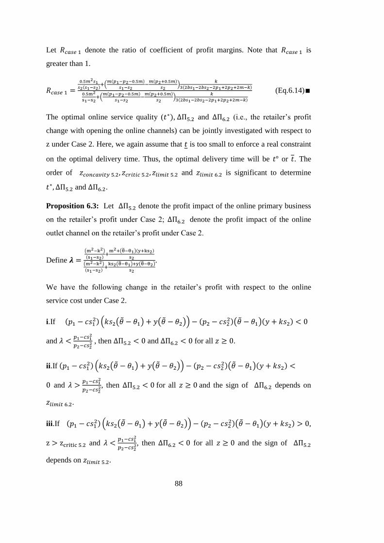
88

Let denote the ratio of coefficient of profit margins. Note that is

greater than 1.

(Eq.6.14)

The optimal online service quality ( , and (i.e., the retailer’s profit

change with opening the online channels) can be jointly investigated with respect to

z under Case 2. Here, we again assume that is too small to enforce a real constraint

on the optimal delivery time. Thus, the optimal delivery time will be or . The

order of and is significant to determine

and .

Proposition 6.3: Let denote the profit impact of the online primary business

on the retailer’s profit under Case 2; denote the profit impact of the online

outlet channel on the retailer’s profit under Case 2.

Define

.

We have the following change in the retailer’s profit with respect to the online

service cost under Case 2.

i.If

and

, then and for all .

ii.If

and

, then for all and the sign of depends on

.

iii.If

,

and

, then for all and the sign of

depends on .

89

iv. If

,

and

, then we may have

a) and

b) and

c) and

d) and depending on the online service cost and

other parameters.

v. If

,

, then for all and

where

where

Proof:

i. We have four feasible orders of the threshold z values. However, independent of

these orders, and for all .

ii. Here, we will have . For all

, and . When , we will have See

Figure I.1 in Appendix I.

iii.Here, we will have . For all

. When , total profit impact of the

90

online channels may or may not be positive. For all , we will have both

and . See Figure I.2 in Appendix I.

iv. Follows similarly to proof of Proposition 6.2(iii).

v. If is plugged into (6.12) in place of optimal promised delivery time,

(Eq.6.15)

(6.15) does not consist of z related term, thus the ratio profit margins determines the

net change in profit.

Let denote the ratio of coefficient of profit margins.

(Eq.6.16)

where

The outlet online channel profitability is determined by two factors: margin ratio

between the primary and the outlet business and the online service cost. When online

service cost is low enough, it ceases to be the limiting factor and the margin ratio

determines profitability. When providing the online service is costly, opening online

channels are not profitable for the retailer at all in both Case 1 and 2. When the

online service cost is moderate (medium level) and the profit margin of the original

91

brand is greater than that of the outlet brand, the profit impact of the primary online

store is always positive, but that of outlet online store can be positive or negative.

When the online service cost is low and the primary brand margin is lower, the profit

impact of the primary online store is positive whereas that of the outlet online store is

negative. This condition may arise when the online service cost is moderate and the

primary brand margin is higher.

Under all cases, generally is larger than . It translates into that the

profit impact of opening online primary store is profitable for markets compared to

that of the online outlet store.

Table 6.2 and 6.3 show summary of Proposition 6.2 and 6.3, respectively.

92

Tab

le 6

.2:

Th

resh

old

val

ues

and o

rder

s of

all

opti

ons

under

Cas

e 1

of

Chap

ter

5 a

nd

6

:

Thre

shold

val

ues

and o

rder

s of

all

opti

ons

for

Cas

e 1 o

f C

hap

ter

5 a

nd

6

Case

1 o

f C

hap

ter

5 a

nd

6

N

ote

if

,

then

.

if

,

then

.

if

,

then

.

If

,th

en

Th

resh

old

val

ues

an

d

ord

er

Ord

er(1

),O

rder

(2),

Ord

e

r(3)

and

Ord

er(4

)

c

on

dit

ion

93

Tab

le 6

.3:

Th

resh

old

val

ues

and o

rder

s of

all

opti

ons

under

Cas

e 2 o

f C

hap

ter

5 a

nd

6

T

hre

sho

ld v

alu

es a

nd

ord

ers

of

all

opti

ons

for

Cas

e 2 o

f C

hap

ter

5 a

nd 6

Case

2 o

f C

hap

ter

5 a

nd

6

N

ote

a

nd

for

all

.

if

, th

en

.

if

, th

en

.

Th

resh

old

v

alu

es

and

ord

er

fou

r fe

asib

le o

rder

s o

f th

e

neg

ativ

e th

resh

old

z v

alu

e

c

on

dit

ion

94

Tab

le 6

. 3

: (cont’d)

Thre

shold

val

ues

and o

rder

s of

all

opti

ons

under

Cas

e 2 o

f C

hap

ter

5 a

nd

6

C

ase

2 o

f C

hap

ter

5 a

nd

6

No

te

if

, th

en

.

If

,th

en

Thre

sho

ld v

alu

es a

nd

ord

er

Ord

er(1

),O

rder

(2),

Ord

er(3

)

and O

rder

(4)

c

on

dit

ion

95

CHAPTER 7

CONCLUSION

This thesis focuses on a monopolist retailer’s product differentiation problem in a

multi-channel environment. We investigate which conditions would motivate retailer

to open an outlet branch, to open an online channel, and to even potentially open an

online channel for the outlet branch, and how these decisions interact with each

other.

In Chapter 3, we characterize how the retailer positions its outlet branch in terms of

quality level and price point and whether he will be better off in terms of total profit.

First, we neglect any inconvenience cost regarding either channel. We demonstrate

that opening the outlet business is preferable for both the retailer and the consumer.

Although the outlet store cannibalizes some of the primary store demand, the retailer

manages to expand its market share and generate more profit through the outlet

business. Also, consumer welfare increases in terms of consumer surplus.

Furthermore, we analyze the type of retailer in terms of the primary brand position

strategies: myopic retailer and non-myopic retailer. In the former strategy, the

retailer can position the primary brand without the any consideration of the outlet

business opportunity in the future. That is, the myopic retailer positions the primary

product and then the outlet product. In the latter one, the retailer also considers the

future outlet product position while positioning the primary product. We show that

non-myopic approach is preferable for the retailer and the non-myopic retailer sets a

higher price and a quality level for the primary brand compared to its myopic

counterpart. In the second part of chapter, we take account inconvenience costs

associated with visiting a brick-and-mortar retailer. This is closer to what happens in

practice. An extensive numerical study is conducted to evaluate the changes (trend)

96

in the outlet product position, demand of primary and outlet business and total profit

of the monopolist brick-and-mortar retailer in the presence of inconvenience cost.

We also find that as the primary brand gets more competitive in terms of quality and

price, the outlet price level tends to be lower. The price competitiveness of the

primary brand does not impact the outlet quality. However, as the primary brand gets

more competitive in terms of quality, it produces the larger market size for the outlet

brand and the outlet quality level tends to be higher. We find that the profit margins

of the primary and outlet business are more significant than market share in

determining the profit of the retailer. We find that as the primary brand gets more

competitive in terms of quality level, its outlet business becomes more robust

(viable) than others.

In Chapter 4, we are interested in a monopolist retailer’s online channel decision.

Through the online channel, consumers are freed from the inconvenience of

physically going to the store and need to wait for a pre-specified time to receive his

product. With the online channel, willingness to wait for products is considered as a

second dimension in addition to their differences in willingness to pay for the

product quality. Under such a setting, we investigate the service quality offered at the

online channel which is the retailer’s main decision. Online service quality may

involve all customer services provided by the online store, promised delivery time

windows as well as shipping charges. We assume that the promised delivery time

can be set in a feasible interval and lower bound is positive since all practically

feasible delivery/service times are in this interval. We find that the retailer achieves

market expansion. However, we find that the profit impact of the online channel on

the retailer’s total profit changes with the online service quality. Explicitly, when

providing online services is not costly, opening an online channel is always

preferable for the retailer. Otherwise, the extra market does not justify the costs of

providing online services.

In Chapter 5, we focus on the service quality offered at the online channel while the

retailer is already selling its original and outlet brand by the respective physical

channels. We determine the three threshold taste parameter values ( ) and that the

two feasible orders (Case 1 and Case 2) among all possible rankings of these taste

parameters. We demonstrate that opening the online channel does not change the

97

total market of the retailer under Case 1 whereas it expands the total market of the

retailer under Case 2. Furthermore, we show that the optimal promised delivery time

and its conditions are different for Case 1 and 2. We find that the profit impact of the

online channel on the retailer’s total profit depends on the feasible interval for online

services, and the online cost parameter in the market.

In Chapter 6, we focus on the profit impact of the online outlet store on the

monopolist retailer’s profit when the retailer already has the primary business with

the physical and online channel and an outlet physical channel. The analysis on

retailer’s profit impact is conducted under two different settings. In the former

setting, the outlet product position and the promised delivery time are taken as

arbitrary; in the latter the optimal promised delivery time found in Chapter 5 is used.

We find that under all cases, opening the online outlet channel expands the retailer’s

total market despite the cannibalization of other channels. When the optimal

promised delivery time found in Chapter 5 is set, we investigate retailer’s profit

change with opening the online channels together with respect to the online cost

parameter. We find that the profitability is determined by the two factors: margin

ratio between the primary and the outlet business and online service cost. When

online service cost is low enough, it ceases to be the limiting factor and margin ratio

determines everything. Explicitly, for each case, when the feasible range of delivery

time is not limiting for the retailer while opening the primary online channel, margin

ratio becomes the critical factor to characterize the total profit impact of the online

outlet channel. Otherwise, threshold value for online service cost determines the

profitability of primary online, outlet online and both.

We limit our work to use the same unit cost coefficient for a given quality

independent of brands. In real life, unit cost of product depends on many factors; i.e.,

material used in the product, dye type, etc. Thus, different unit cost coefficients may

be defined for the primary and outlet brand. We also assume that there are no fixed

costs. However, different fixed costs may be associated the physical and online

channel.

In Chapter 6, we assume, to remain consistent with the practice, opening the primary

online store and online outlet are sequential events. However, the profit impact of the

98

online channels on the retailer’s total profit is evaluated in the same online service

cost environment. This part of work can be extended to do the same analysis with a

changing the online service cost parameter over time.

99

REFERENCES

Berman, B., Evans, J.R., Retail Management: A Strategic Approach, 10th Ed.,

Pearson Prentice Hall, USA. 2006

Levy, M., Weitz, B.A., Retailing Management, 3rd Ed., Richard D. Irwin Inc., USA,

2012

www.jcrew.com/help/about jcrew.jsp, Last visited on October 2014

Shy, O., Industrial Organization: Theory and Applications, 2nd Ed., The MIT Press,

England, 1996

Hotelling, H., 1929,” Stability in Competition”, The Economic Journal, 39, 41-57.

d’Aspremont, C., Gabszewicz, J.,Thisse, J.,1979, Econometrica,On Hotelling’s

Stability in Competition, 47,1145-1150.

Moorthy, K.S., 1988, Marketing Science, Product and Price Competition in Duopoly,

Vol. 7, No. 2, 141-168.

Moorthy, K.S., 1984, Marketing Science, Market Segmentation, Self-Selection, and

Product Line Design, Vol.3, No.4, 288-307.

Moorthy, K.S., 1987, Ann. Telecommun., Product Line Competition, 42, 11-12,655-

663.

Moorthy, K.S., Png, I.P.L., 1992, Management Science, Market Segmentation,

Cannibalization and the Timing of the Product Introductions, Vol.38, No.3, 345-359.

Purohit, D., 1994, Marketing Science, What Should You Do When Your

Competitors Send in the Clones?, Vol.13, No.4, 392-411.

Vandenbosch, M.B., Weinberg, C.B., 1995, Marketing Science, Product and Price

Competition in a Two-Dimensional Vertical Differentiation Model, Vol. 14, No. 2,

224-249.

http://www.jcrew.com/help/about%20jcrew.jsp

100

Lauga, D.O., Ofek, E., 2011, Marketing Science, Product Positioning in a Two-

Dimensional Vertical Differentiation Model: The Role of Quality Costs, Vol. 30, No.

5, 903–923.

Desai, S.P., 2001, Marketing Science, Quality Segmentation in Spatial Markets:

When Does Cannibalization Affect Product Line Design?, Vol. 20, No. 3, 265–283.

Kim, K., Dilip, C., Liu, Y., 2013, Marketing Science, Can Commonality Relieve

Cannibalization in Product Line Design?, Vol.32, No.3, 510-521.

Ferguson, M.E., Koenigsberg, O., 2007, Production and Operations Management,

How Should a Firm Manage Deteriorating Inventory?, Vol.16, No.3, 306-321.

Chen, K., Kaya, M., Özer,Ö., 2008, Manufacturing & Service Operations

Management, Dual Sales Channel Management with Service Competition, Vol.10,

No.4, 654-675.

Tsay, A.A., Agrawal, N., 2004, Production and Operations Management, Channel

Conflict and Coordination in the E-Commerce Age, Vol.13, No.1, 93-110.

Zhang, X., 2009, Marketing Science, Retailers’ Multichannel and Price Advertising

Strategies, Vol.28, No.6, 1080-1094.

Bernstein, F., Song, J., Zheng, X., 2008, European Journal of Operational, ‘‘Bricks-

and-mortar’’ vs. ‘‘Clicks-and-mortar’’:An Equilibrium Analysis, 187,671-690.

Coughlan, A.T., Soberman, A.D., 2005, J. of Research in Marketing, Strategic

Segmentation Using Outlet Malls, Vol. 22, 61-86.

Liu, Y., Gupta,S., Zhang, Z.J.,2006, Marketing Science, Note on Self-Restraint as an

Online Entry-Deterrence Strategy, Vol.52, No.11, 1799-1809.

Balasubramanian, S., 1998, Marketing Science, Mail versus Mall: A Strategic

Analysis of Competition between Direct Marketers and Conventional Retailers,

Vol.17, No.3, 181-195

101

APPENDIX A

NUMERICAL ANALYSIS FOR TRIAL 2

Table A. 1: s2*, p2

*, D1

*, D2

* retailer’s profit and total market and profit margin of the

outlet for trial 2 when k=0.5

k m

Profit

Total

Market

0.5 0.5 4.56 4.81 38.491 0.343 139.508 38.835 2.730

0.5 0.6 4.51 4.69 38.506 0.321 139.475 38.827 2.655

0.5 0.7 4.49 4.61 38.5217 0.295 139.444 38.817 2.593

0.5 0.8 4.47 4.54 38.537 0.269 139.416 38.806 2.541

0.5 0.9 4.45 4.46 38.552 0.242 139.391 38.795 2.479

0.5 1 4.43 4.39 38.567 0.216 139.368 38.784 2.427

0.5 1.1 4.42 4.32 38.582 0.190 139.347 38.772 2.366

0.5 1.2 4.4 4.25 38.596 0.164 139.329 38.761 2.314

0.5 1.3 4.39 4.19 38.611 0.139 139.314 38.750 2.262

0.5 1.4 4.38 4.12 38.625 0.113 139.301 38.738 2.201

0.5 1.5 4.33 4 38.637 0.092 139.291 38.730 2.125

0.5 1.6 4.32 3.94 38.651 0.067 139.283 38.718 2.073

102

Table A.1: (cont’d) s2*, p2

*, D1

*, D2

* retailer’s profit and total market and profit

margin of the outlet for trial 2 when k=0.5

k m

Profit

Total

Market

0.5 1.7 4.3 3.86 38.665 0.041 139.278 38.706 2.011

0.5 1.8 4.28 3.79 38.679 0.015 139.275 38.694 1.958

0.5 1.9 0 0 38.687 0 139.275 38.687 0

0.5 2 0 0 38.687 0 139.275 38.687 0

0.5 2.1 0 0 38.687 0 139.275 38.687 0

0.5 2.2 0 0 38.687 0 139.275 38.687 0

0.5 2.3 0 0 38.687 0 139.275 38.687 0

0.5 2.4 0 0 38.687 0 139.275 38.687 0

0.5 2.5 0 0 38.687 0 139.275 38.687 0

0.5 2.6 0 0 38.687 0 139.275 38.687 0

0.5 2.7 0 0 38.687 0 139.275 38.687 0

0.5 2.8 0 0 38.687 0 139.275 38.687 0

0.5 2.9 0 0 38.687 0 139.275 38.687 0

0.5 3 0 0 38.687 0 139.275 38.687 0

Figure A.1: D1* versus m plot for trial 2 when k=0.5

38.35

38.4

38.45

38.5

38.55

38.6

38.65

38.7

38.75

0.5 0.7 0.9 1.1 1.3 1.5 1.7 1.9 2.1 2.3 2.5 2.7 2.9

De

man

d o

f th

e p

rim

ary

bra

nd

(D

1)

m

103

Figure A.2: D2* versus m plot for trial 2 when k=0.5

Figure A.3: Retailer’s profit versus m plot for trial 2 when k=0.5

0

0.05

0.1

0.15

0.2

0.25

0.3

0.35

0.5 0.7 0.9 1.1 1.3 1.5 1.7 1.9 2.1 2.3 2.5 2.7 2.9

De

man

d o

f th

e o

utl

et

bra

nd

(D

2)

m

139.15

139.2

139.25

139.3

139.35

139.4

139.45

139.5

139.55

0.5 0.7 0.9 1.1 1.3 1.5 1.7 1.9 2.1 2.3 2.5 2.7 2.9

Re

taile

r's

pro

fit

m

104

Figure A.4: Retailer’s total market share versus m plot for trial 2 when k=0.5

Figure A.5: (p2-c(s2*)

2) versus m plot for trial 2 when k=0.5

38.65

38.7

38.75

38.8

38.85

0.5 0.7 0.9 1.1 1.3 1.5 1.7 1.9 2.1 2.3 2.5 2.7 2.9

Re

taile

r's

tota

l mar

ket

m

0

0.5

1

1.5

2

2.5

3

0.5 0.7 0.9 1.1 1.3 1.5 1.7 1.9 2.1 2.3 2.5 2.7 2.9

P.m

argi

n o

f o

utl

et

m

105

APPENDIX B

NUMERICAL ANALYSIS FOR TRIAL 1

Table B.1: s2*, p2

*, D1

*, D2

* ,retailer’s profit for trial 1 when m=k

k m

Profit

0 0 4 3.2 38.800 0.400 62.720

0.1 0.1 4.12 3.3 38.788 0.386 62.680

0.2 0.2 4.24 3.4 38.776 0.374 62.642

0.3 0.3 4.35 3.49 38.764 0.364 62.605

0.4 0.4 4.45 3.57 38.752 0.355 62.568

0.5 0.5 4.55 3.66 38.742 0.343 62.533

0.6 0.6 4.66 3.76 38.730 0.333 62.499

0.7 0.7 4.73 3.81 38.718 0.327 62.465

0.8 0.8 4.84 3.92 38.708 0.315 62.432

0.9 0.9 4.92 3.99 38.698 0.308 62.400

1 1 4.99 4.05 38.687 0.300 62.368

1 1 4.99 4.05 38.687 0.300 62.368

1.1 1.1 5.09 4.15 38.676 0.291 62.337

106

Table B.1: (cont’d) s2*, p2

*, D1

*, D2

* retailer’s profit for trial 1

when m=k

k m

Profit

1.2 1.2 5.15 4.2 38.666 0.284 62.307

1.3 1.3 5.23 4.28 38.657 0.276 62.277

1.4 1.4 5.31 4.36 38.646 0.268 62.248

1.5 1.5 5.39 4.44 38.636 0.261 62.219

1.6 1.6 5.45 4.50 38.627 0.253 62.191

1.7 1.7 5.55 4.61 38.616 0.246 62.163

1.8 1.8 5.61 4.67 38.606 0.240 62.136

1.9 1.9 5.66 4.72 38.598 0.232 62.109

2 2 5.74 4.81 38.588 0.225 62.082

2.1 2.1 5.82 4.9 38.577 0.219 62.056

2.2 2.2 5.87 4.95 38.568 0.213 62.030

2.3 2.3 5.93 5.02 38.560 0.205 62.005

2.4 2.4 6.00 5.10 38.550 0.200 61.980

2.5 2.5 6.06 5.17 38.541 0.193 61.955

2.6 2.6 6.12 5.24 38.531 0.187 61.930

2.7 2.7 6.18 5.31 38.521 0.181 61.906

2.8 2.8 6.23 5.37 38.514 0.174 61.882

2.9 2.9 6.31 5.47 38.502 0.170 61.858

3 3 6.36 5.53 38.493 0.164 61.835

107

Figure B.1: s2* versus m plot for trial 1 when m=k

Figure B.2: p2* versus m plot for trial 1 when m=k

3.5

4

4.5

5

5.5

6

6.5

7

0 0.2 0.4 0.6 0.8 1 1.2 1.4 1.6 1.8 2 2.2 2.4 2.6 2.8 3

Ou

tle

t q

ual

ity

(s2

)

m

2.5

3

3.5

4

4.5

5

5.5

6

0 0.2 0.4 0.6 0.8 1 1.2 1.4 1.6 1.8 2 2.2 2.4 2.6 2.8 3

Ou

tle

t p

rice

(p

2)

m

108

Figure B.3: D1* versus m plot for trial 1 when m=k

Figure B.4: D2* versus m plot for trial 1 when m=k

38.3

38.35

38.4

38.45

38.5

38.55

38.6

38.65

38.7

38.75

38.8

38.85

0 0.2 0.4 0.6 0.8 1 1.2 1.4 1.6 1.8 2 2.2 2.4 2.6 2.8 3

De

man

d o

f th

e p

rim

ary

bra

nd

(D

1)

m

0

0.05

0.1

0.15

0.2

0.25

0.3

0.35

0.4

0.45

0 0.2 0.4 0.6 0.8 1 1.2 1.4 1.6 1.8 2 2.2 2.4 2.6 2.8 3

De

man

d o

f th

e o

utl

et

bra

nd

(D

2)

m

109

APPENDIX C

NUMERICAL ANALYSIS FOR THE FIRST GROUP TRIALS

Figure C.1: D1* for the first group of trials when k=0.3

37.4

37.6

37.8

38

38.2

38.4

38.6

38.8

39

39.2

0.3 0.5 0.7 0.9 1.1 1.3 1.5 1.7 1.9 2.1 2.3 2.5 2.7 2.9

De

man

d o

f th

e p

rim

ary

bra

nd

(D

1)

m





110

111

APPENDIX D

NUMERICAL ANALYSIS FOR THE SECOND GROUP TRIALS

Figure D.1: D1* for the second group of trials when k=0.3

Figure D.2: Retailer’s market share for the second group of trials when k=0.3

35.5

36

36.5

37

37.5

38

38.5

39

39.5

40

0.3 0.5 0.7 0.9 1.1 1.3 1.5 1.7 1.9 2.1 2.3 2.5 2.7 2.9

De

man

d o

f th

e p

rim

ary

bra

nd

(D

1)

m





35

35.5

36

36.5 37

37.5 38

38.5

39 39.5

0.3 0.5 0.7 0.9 1.1 1.3 1.5 1.7 1.9 2.1 2.3 2.5 2.7 2.9

Re

taile

r's

tota

l mar

ket

m

Retailer's total market for trial 5 Retailer's total market for trial 6 Retailer's total market for trial 7 Retailer's total market for trial 8

112

113

APPENDIX E

LEMMA 4.2

Lemma 4.2: There are two feasible orders for the threshold z values: Order 1;

i.e.; and Order 2; i.e.;

.

Proof: It is clear that is satisfied. If

holds, then is satisfied and consequently Order 1

occurs. Otherwise, Order 2 occurs. Note that is used for choosing the optimal

promised delivery time with min and calculating .

114

115

APPENDIX F

PROPOSITION 5.4

Proposition 5.4: We have the following conditions in retailer’s profit and optimal

promised delivery time with respect to the online service cost under Case 1

(i.e., .

i. If

, then and for all .

ii.If

, then there are two feasible orders for the

threshold z values (i.e., Order 1 and 2). For all order, the profit impact of the online

channel on the retailer’s profit change with . The optimal promised delivery

time will be or t for Order 1, however it will be or t for Order 2.

Proof:

i.See proof of Proposition 5.2(i).

ii. When

, then there are two feasible orders for the

threshold z values: Order 1; i.e.,

and Order 2; i.e., .It

is clear that is satisfied. If

holds,

then holds and consequently Order 1 occurs. Otherwise,

Order 2 occurs.

116

Figure F.1: t*, ∆∏5.1 for Order 1 under Case 1

Figure F.2: t*, ∆∏5.1 for Order 2 under Case 1

117

APPENDIX G

PROPOSITION 5.5

Proposition 5.5: We have the following conditions in retailer’s profit and optimal

promised delivery time with respect to the online service cost under Case 2

(i.e., )

i. If

and for all .

ii.If

then there are two feasible orders for the threshold z values (i.e., Order 1 and 2). For

all order, the profit impact of the online channel on the retailer’s profit change with

. The optimal promised delivery time will be or t for Order 1, however it

will be or t for Order 2.

Proof:

i.See proof of Proposition 5.3(i).

ii. When

, then there are two feasible orders for the threshold z values: Order 1; i.e.,

and Order 2; i.e.,

where

.

118

It is clear that is satisfied. If

holds,

then holds and consequently Order 1 occurs. Otherwise,

Order 2 occurs.

Figure G.3: t*, ∆∏5.2 for Order 1 under Case 2

Figure G.4: t*, ∆∏5.2 for Order 2 under Case 2

119

APPENDIX H

PROOF OF PROPOSITION 6.2

i.

Figure H.1: t*, ∆∏5.1, ∆∏6.1 when (p1-c1

2)-(p2-s2

2)<0

ii.

Figure H.2: t*, ∆∏5.1, ∆∏6.1 when (p1-c1

2)-(p2-s2

2)>0 and zlimit 6.1<0

iii. Order (1)

Figure H.3: t*, ∆∏5.1, ∆∏6.1 for Order (1)

120

Order (2)

Figure H.4: t*, ∆∏5.1, ∆∏6.1 for Order (2)

Order (3) and (4)

Figure H.5: t*, ∆∏5.1, ∆∏6.1 for Order (3) and Order (4)

121

APPENDIX I

PROOF OF PROPOSITION 6.3

ii.

Figure I.1: t*, ∆∏5.2, ∆∏6.2 for Proposition 6.3(ii)

iii.

Figure I.2: t*, ∆∏5.2, ∆∏6.2 for Proposition 6.3(iii)

122

Documents

MULTI-CHANNEL RETAILING WITH PRODUCT …etd.lib.metu.edu.tr/upload/12618472/index.pdf · i multi-channel retailing with product differentiation a thesis submitted to the graduate