Embed Size (px)
Citation preview


Mukund R. Patel, Ph.D., P.E.U.S. Merchant Marine Academy
Kings Point, New York
FormerlyPrincipal Engineer, General Electric Company
Fellow Engineer, Westinghouse Reasearch Center
Wind and SolarPower Systems
Boca Raton London New York Washington, D.C.CRC Press

Library of Congress Cataloging-in-Publication Data
Patel, Mukind R., 1942.Wind and solar power systems / Mukund R. Patel.
p. cm.Includes bibliographical references and index.ISBN 0-8493-1605-7 (alk. paper)1. Wind power plants. 2. Solar power plants. 3. Photovoltaic power systems. I. Title.
TK1541.P38 1999621.31
′
2136—dc21 98-47934CIP
This book contains information obtained from authentic and highly regarded sources. Reprinted materialis quoted with permission, and sources are indicated. A wide variety of references are listed. Reasonableefforts have been made to publish reliable data and information, but the author and the publisher cannotassume responsibility for the validity of all materials or for the consequences of their use.
Neither this book nor any part may be reproduced or transmitted in any form or by any means, electronicor mechanical, including photocopying, microfilming, and recording, or by any information storage orretrieval system, without prior permission in writing from the publisher.
The consent of CRC Press LLC does not extend to copying for general distribution, for promotion, forcreating new works, or for resale. Specific permission must be obtained in writing from CRC Press LLCfor such copying.
Direct all inquiries to CRC Press LLC, 2000 N.W., Corporate Blvd., Boca Raton, Florida 33431.
Trademark Notice:
Product or corporate names may be trademarks or registered trademarks, and are used only for identification and explanation, without intent to infringe.
Visit the CRC Press Web site at www.crcpress.com
© 1999 by CRC Press LLC
No claim to original U.S. Government worksInternational Standard Book Number 0-8493-1605-7
Library of Congress Card Number 98-47934Printed in the United States of America 2 3 4 5 6 7 8 9 0
Printed on acid-free paper

© 1999 by CRC Press LLC
…dedicated
to my mother, Shakariba,
who practiced ingenuity,
and
to my children, Ketan, Bina, and Vijal,
who flattered me by being engineers.
(Cover photo: Baix Ebre wind farm in Catalonia. With permission fromInstitut Catalia d’Energia, Spain.)

© 1999 by CRC Press LLC
Preface
The total electricity demand in 1997 in the United States of America wasthree trillion kWh, with the market value of $210 billion. The worldwidedemand was 12 trillion kWh in 1997, and is projected to reach 19 trillionkWh in 2015. This constitutes the worldwide average annual growth of2.6 percent. The growth rate in the developing countries is projected to beapproximately 5 percent, almost twice the world average.
Most of the present demand in the world is met by fossil and nuclear powerplants. A small part is met by renewable energy technologies, such as thewind, solar, biomass, geothermal and the ocean. Among the renewable powersources, wind and solar have experienced a remarkably rapid growth in thepast 10 years. Both are pollution free sources of abundant power. Additionally,they generate power near the load centers, hence eliminate the need of run-ning high voltage transmission lines through rural and urban landscapes.
Since the early 1980s, the wind technology capital costs have declined by80 percent, operation and maintenance costs have dropped by 80 percentand availability factors of grid-connected plants have risen to 95 percent.These factors have jointly contributed to the decline of the wind electricitycost by 70 percent to 5 to 7 cents per kWh. The grid-connected wind plantcan generate electricity at cost under 5 cents per kWh. The goal of ongoingresearch programs funded by the U.S. Department of Energy and theNational Renewable Energy Laboratory is to bring the wind power costbelow 4 cents per kWh by the year 2000. This cost is highly competitive withthe energy cost of the conventional power technologies. For these reasons,wind power plants are now supplying economical clean power in manyparts of the world.
In the U.S.A., several research partners of the NREL are negotiating withU.S. electrical utilities to install additional 4,200 MW of wind capacity withcapital investment of about $2 billion during the next several years. Thisamounts to the capital cost of $476 per kW, which is comparable with theconventional power plant costs. A recent study by the Electric PowerResearch Institute projected that by the year 2005, wind will produce thecheapest electricity available from any source. The EPRI estimates that thewind energy can grow from less than 1 percent in 1997 to as much as10 percent of this country’s electrical energy demand by 2020.
On the other hand, the cost of solar photovoltaic electricity is still high inthe neighborhood of 15 to 25 cents per kWh. With the consumer cost ofelectrical utility power ranging from 10 to 15 cents per kWh nationwide,photovoltaics cannot economically compete directly with the utility poweras yet, except in remote markets where the utility power is not available and

© 1999 by CRC Press LLC
the transmission line costs would be prohibitive. Many developing countrieshave large areas falling in this category. With ongoing research in the pho-tovoltaic (pv) technologies around the world, the pv energy cost is expectedto fall to 12 to 15 cents per kWh or less in the next several years as thelearning curves and the economy of scale come into play. The researchprograms funded by DOE/NREL have the goal of bringing down the pvenergy cost below 12 cents per kWh by 2000.
After the restructuring of the U.S. electrical utilities, as mandated by theEnergy Policy Act (EPAct) of 1992, the industry leaders expect the powergeneration business, both conventional and renewable, to become more prof-itable in the long run. The reasoning is that the generation business will bestripped of regulated price and opened to competition among electricityproducers and resellers. The transmission and distribution business, on theother hand, would still be regulated. The American experience indicates thatthe free business generates more profits than the regulated business. Suchis the experience in the U.K. and Chile, where the electrical power industryhad been structured similar to the EPAct of 1992 in the U.S.A.
As for the wind and pv electricity producers, they can now sell powerfreely to the end users through truly open access to the transmission lines.For this reason, they are likely to benefit as much as other producers ofelectricity. Another benefit in their favor is that the cost of the renewableenergy would be falling as the technology advances, whereas the cost of theelectricity from the conventional power plants would rise with inflation. Thedifference in their trends would make the wind and pv power even moreadvantageous in the future.

© 1999 by CRC Press LLC
About the Author
Mukund R. Patel, Ph.D, P.E.
, is an experienced research engineer with35 years of hands-on involvement in designing and developing state-of-the-art electrical power equipment and systems. He has served as principalpower system engineer at the General Electric Company in Valley Forge,fellow engineer at the Westinghouse Research & Development Center inPittsburgh, senior staff engineer at Lockheed Martin Corporation in Prince-ton, development manager at Bharat Bijlee Limited, Bombay, and 3M dis-tinguished visiting professor of electrical power technologies at theUniversity of Minnesota, Duluth. Presently he is a professor at the U.S.Merchant Marine Academy in Kings Point, New York.
Dr. Patel obtained his Ph.D. degree in electric power engineering from theRensselaer Polytechnic Institute, Troy, New York; M.S. in engineering man-agement from the University of Pittsburgh; M.E. in electrical machine designfrom Gujarat University and B.E.E. from Sardar University, India. He is afellow of the Institution of Mechanical Engineers (U.K.), senior member ofthe IEEE, registered professional engineer in Pennsylvania, and a memberof Eta Kappa Nu, Tau Beta Pi, Sigma Xi and Omega Rho.
Dr. Patel has presented and published over 30 papers at national andinternational conferences, holds several patents, and has earned NASA rec-ognition for exceptional contribution to the photovoltaic power systemdesign for UARS. He is active in consulting and teaching short courses toprofessional engineers in the electrical power industry.
© 1999 by CRC Press LLC
About the Book
The book was conceived when I was invited to teach a course in the emergingelectrical power technologies at the University of Minnesota in Duluth. Thelecture notes and presentation charts I prepared for the course formed thefirst draft of the book. The subsequent teaching of a couple of short coursesto professional engineers advanced the draft closer to the finished book. Thebook is designed and tested to serve as textbook for a semester course foruniversity seniors in electrical and mechanical engineering fields. The prac-ticing engineers will get detailed treatment of this rapidly growing segmentof the power industry. The government policy makers would benefit byoverview of the material covered in the book.
Chapters 1 through 3 cover the present status and the ongoing researchprograms in the renewable power around the world and in the U.S.A.Chapter 4 is a detailed coverage on the wind power fundamentals and theprobability distributions of the wind speed and the annual energy potentialof a site. It includes the wind speed and energy maps of several countries.Chapter 5 covers the wind power system operation and the control require-ments. Since most wind plants use induction generators for converting theturbine power into electrical power, the theory of the induction machineperformance and operation is reviewed in Chapter 6 without going intodetails. The details are left for the classical books on the subject. The electricalgenerator speed control for capturing the maximum energy under windfluctuations over the year is presented in Chapter 7.
The power-generating characteristics of the photovoltaic cell, the arraydesign, and the sun-tracking methods for the maximum power generationare discussed in Chapter 8. The basic features of the utility-scale solar ther-mal power plant using concentrating heliostats and molten salt steam turbineare presented in Chapter 9.
The stand-alone renewable power plant invariably needs energy storagefor high load availability. Chapter 10 covers characteristics of various bat-teries, their design methods using the energy balance analysis, factors influ-encing their operation, and the battery management methods. The energydensity and the life and operating cost per kWh delivered are presented forvarious batteries, such as lead-acid, nickel-cadmium, nickel-metal-hydrideand lithium-ion. The energy storage by the flywheel, compressed air and thesuperconducting coil, and their advantages over the batteries are reviewed.The basic theory and operation of the power electronic converters and invert-ers used in the wind and solar power systems are presented in Chapter 11,leaving details for excellent books available on the subject.

© 1999 by CRC Press LLC
The more than two billion people in the world not yet connected to theutility grid are the largest potential market of stand-alone power systems.Chapter 12 presents the design and operating methods of such power sys-tems using wind and photovoltaic systems in hybrid with diesel generators.The newly developed fuel cell with potential of replacing diesel engine inurban areas is discussed. The grid-connected renewable power systems arecovered in Chapter 13, with voltage and frequency control methods neededfor synchronizing the generator with the grid. The theory and the operatingcharacteristics of the interconnecting transmission line, the voltage regula-tion, the maximum power transfer capability, and the static and dynamicstability are covered.
Chapter 14 is about the overall electrical system design. The method ofdesigning the system components to operate at their maximum possibleefficiency is developed. The static and dynamic bus performance, the har-monics, and the increasingly important quality of power issues applicableto the renewable power systems are presented.
Chapter 15 discusses the total plant economy and the costing of energydelivered to the paying customers. It also shows the importance of a sensi-tivity analysis to raise confidence level of the investors. The profitabilitycharts are presented for preliminary screening of potential sites. Finally,Chapter 16 discusses the past and present trends and the future of the greenpower. It presents the declining price model based on the learning curve,and the Fisher-Pry substitution model for predicting the market growth ofthe wind and pv power based on historical data on similar technologies. Theeffect of the utility restructuring, mandated by the EPAct of 1992, and itsexpected benefits on the renewable power producers are discussed.
At the end, the book gives numerous references for further reading, andname and addresses of government agencies, universities, and manufactur-ers active in the renewable power around the world.

© 1999 by CRC Press LLC
Acknowledgment
The book of this nature on emerging technologies, such as the wind andphotovoltaic power systems, cannot possibly be written without the helpfrom many sources. I have been extremely fortunate to receive full supportfrom many organizations and individuals in the field. They not only encour-aged me to write the book on this timely subject, but also provided valuablesuggestions and comments during the development of the book.
Dr. Nazmi Shehadeh
, head of the Electrical and Computer EngineeringDepartment at the University of Minnesota, Duluth, gave me the opportunityto develop and teach this subject to his students who were enthusiastic aboutlearning new technologies.
Dr. Elliott Bayly
, president of the World PowerTechnologies in Duluth, shared with me and my students his long experiencein the field. He helped me develop the course outline, which later becamethe book outline.
Dr. Jean Posbic
of Solarex Corporation in Frederick, Mary-land and
Mr. Carl-Erik Olsen
of Nordtank Energy Group/NEG Micon,Denmark, kindly reviewed the draft and provided valuable suggestions forimprovement.
Mr. Bernard Chabot
of ADEME, Valbonne, France, providedthe profitability charts for screening the wind and photovoltaic power sites.
Mr. Ian Baring-Gould
of the National Renewable Energy Laboratory,Golden, Colorado, has been a source of useful information and the hybridpower plant simulation model.
Several institutions worldwide provided current data and reports on theserather rapidly developing technologies. They are the
American Wind EnergyAssociation
, the
American Solar Energy Society
, the
European WindEnergy Association
, the
Risø National Laboratory
, Denmark, the
TataEnergy Research Institute
, India, and many corporations engaged in thewind and solar power technologies. Many individuals at these organizationsgladly provided help I requested.
I gratefully acknowledge the generous support from all of you.
Mukund PatelYardley, Pennsylvania

© 1999 by CRC Press LLC
Contents
1. Introduction
1.1 Industry Overview1.2 Incentives for Renewables1.3 Utility Perspective
1.3.1 Modularity1.3.2 Emission-Free
References
2. Wind Power
2.1 Wind in the World2.2 The U.S.A.2.3 Europe2.4 India2.5 Mexico2.6 Ongoing Research and DevelopmentReferences
3. Photovoltaic Power
3.1 Present Status3.2 Building Integrated pv Systems3.3 pv Cell Technologies
3.3.1 Single-Crystalline Silicon3.3.2 Polycrystalline and Semicrystalline3.3.3 Thin Films3.3.4 Amorphous Silicon3.3.5 Spheral3.3.6 Concentrated Cells
3.4 pv Energy MapsReferences
4. Wind Speed and Energy Distributions
4.1 Speed and Power Relations4.2 Power Extracted from the Wind4.3 Rotor Swept Area4.4 Air Density4.5 Global Wind Patterns4.6 Wind Speed Distribution
4.6.1 Weibull Probability Distribution4.6.2 Mode and Mean Speeds

© 1999 by CRC Press LLC
4.6.3 Root Mean Cube Speed4.6.4 Mode, Mean, and rmc Speeds Compared4.6.5 Energy Distribution4.6.6 Digital Data Loggers4.6.7 Effect of Height4.6.8 Importance of Reliable Data
4.7 Wind Speed Prediction4.8 Wind Resource Maps
4.8.1 The U.S.A.4.8.2 Minnesota4.8.3 The United Kingdom4.8.4 Europe4.8.5 Mexico4.8.6 India
References
5. Wind Power System
5.1 System Components5.1.1 Tower5.1.2 Turbine Blades5.1.3 Yaw Control5.1.4 Speed Control
5.2 Turbine Rating5.3 Electrical Load Matching5.4 Variable-Speed Operation5.5 System Design Features
5.5.1 Number of Blades5.5.2 Rotor Upwind or Downwind5.5.3 Horizontal Axis Versus Vertical Axis5.5.4 Spacing of the Towers
5.6 Maximum Power Operation5.6.1 Constant Tip-Speed Ratio Scheme5.6.2 Peak Power Tracking Scheme
5.7 System Control Requirements5.7.1 Speed Control5.7.2 Rate Control
5.8 Environmental Aspects5.8.1 Audible Noise5.8.2 Electromagnetic Interference (EMI)
References
6. Electrical Generator
6.1 Electromechanical Energy Conversion6.1.1 DC Machine6.1.2 Synchronous Machine6.1.3 Induction Machine

© 1999 by CRC Press LLC
6.2 Induction Generator6.2.1 Construction6.2.2 Working Principle6.2.3 Rotor Speed and Slip6.2.4 Equivalent Circuit for Performance Calculations6.2.5 Efficiency and Cooling6.2.6 Self-Excitation Capacitance6.2.7 Torque-Speed Characteristic6.2.8 Transients
References
7. Generator Drives
7.1 Speed Control Regions7.2 Generator Drives
7.2.1 One Fixed-Speed Drive7.2.2 Two Fixed-Speeds Drive7.2.3 Variable-Speed Using Gear Drive7.2.4 Variable-Speed Using Power Electronics7.2.5 Scherbius Variable-Speed Drive7.2.6 Variable-Speed Direct Drive
7.3 Drive Selection7.4 Cut-Out Speed SelectionReferences
8. Solar Photovoltaic Power System
8.1 The pv Cell8.2 Module and Array8.3 Equivalent Electrical Circuit8.4 Open Circuit Voltage and Short Circuit Current8.5 i-v and p-v Curves8.6 Array Design
8.6.1 Sun Intensity8.6.2 Sun Angle8.6.3 Shadow Effect8.6.4 Temperature Effect8.6.5 Effect of Climate8.6.6 Electrical Load Matching8.6.7 Sun Tracking
8.7 Peak Power Point Operation8.8 pv System ComponentsReferences
9. Solar Thermal System
9.1 Energy Collection9.1.1 Parabolic Trough9.1.2 Central Receiver9.1.3 Parabolic Dish

© 1999 by CRC Press LLC
9.2 Solar II Power Plant9.3 Synchronous Generator
9.3.1 Equivalent Electrical Circuit9.3.2 Excitation Methods9.3.3 Electrical Power Output9.3.4 Transient Stability Limit
9.4 Commercial Power PlantsReferences
10. Energy Storage
10.1 Battery10.2 Types of Batteries
10.2.1 Lead-Acid10.2.2 Nickel Cadmium10.2.3 Nickel-Metal Hydride10.2.4 Lithium-Ion10.2.5 Lithium-Polymer10.2.6 Zinc-Air
10.3 Equivalent Electrical Circuit10.4 Performance Characteristics
10.4.1 Charge/Discharge Voltages10.4.2 Charge/Discharge Ratio10.4.3 Energy Efficiency10.4.4 Internal Resistance10.4.5 Charge Efficiency10.4.6 Self-Discharge and Trickle Charge10.4.7 Memory Effect10.4.8 Effects of Temperature10.4.9 Internal Loss and Temperature Rise10.4.10 Random Failure10.4.11 Wear-Out Failure10.4.12 Various Batteries Compared
10.5 More on Lead-Acid Battery10.6 Battery Design10.7 Battery Charging10.8 Charge Regulators
10.8.1 Multiple Charge Rates10.8.2 Single Charge Rate10.8.3 Unregulated Charging
10.9 Battery Management10.9.1 Monitoring and Controls10.9.2 Safety
10.10 Flywheel10.10.1 Energy Relations10.10.2 Flywheel System Components10.10.3 Flywheel Benefits Over Battery

© 1999 by CRC Press LLC
10.11 Compressed Air10.12 Superconducting CoilReferences
11. Power Electronics
11.1 Basic Switching Devices11.2 AC to DC Rectifier11.3 DC to AC Inverter11.4 Grid Interface Controls
11.4.1 Voltage Control11.4.2 Frequency Control
11.5 Battery Charge/Discharge Converters11.5.1 Battery Charge Converter11.5.2 Battery Discharge Converter
11.6 Power ShuntsReferences
12. Stand-Alone System
12.1 pv Stand-Alone12.2 Electric Vehicle12.3 Wind Stand-Alone12.4 Hybrid System
12.4.1 Hybrid with Diesel12.4.2 Hybrid with Fuel Cell12.4.3 Mode Controller12.4.4 Load Sharing
12.5 System Sizing12.5.1 Power and Energy Estimates12.5.2 Battery Sizing12.5.3 pv Array Sizing
12.6 Wind Farm SizingReferences
13. Grid-Connected System
13.1 Interface Requirements13.2 Synchronizing with Grid
13.2.1 Inrush Current13.2.2 Synchronous Operation13.2.3 Load Transient13.2.4 Safety
13.3 Operating Limit13.3.1 Voltage Regulation13.3.2 Stability Limit
13.4 Energy Storage and Load Scheduling13.5 Utility Resource Planning ToolReferences

© 1999 by CRC Press LLC
14. Electrical Performance
14.1 Voltage Current and Power Relations14.2 Component Design for Maximum Efficiency14.3 Electrical System Model14.4 Static Bus Impedance and Voltage Regulation14.5 Dynamic Bus Impedance and Ripple14.6 Harmonics14.7 Quality of Power
14.7.1 Harmonic Distortion14.7.2 Voltage Transients and Sags14.7.3 Voltage Flickers
14.8 Renewable Capacity Limit14.8.1 Systems Stiffness14.8.2 Interfacing Standards
14.9 Lightning Protection14.10 National Electrical Code
®
on Renewable Power SystemsReferences
15. Plant Economy
15.1 Energy Delivery Factor15.2 Initial Capital Cost15.3 Availability and Maintenance15.4 Energy Cost Estimates15.5 Sensitivity Analysis
15.5.1 Effect of Wind Speed Variations15.5.2 Effect of Tower Height
15.6 Profitability Index15.6.1 Wind Farm Screening Chart15.6.2 pv Park Screening Chart15.6.3 Stand-Alone pv Versus Grid Line
15.7 Hybrid EconomicsReferences
16. The Future
16.1 World Electricity Demand to 201516.2 Wind Future16.3 pv Future16.4 Declining Production Costs16.5 Market Penetration16.6 Effect of Utility Restructuring
16.6.1 Energy Policy Act of 199216.6.2 Impact on Renewable Power Producers
References
Further ReadingAppendix 1

© 1999 by CRC Press LLC
Appendix 2AcronymsConversion of Units

© 1999 by CRC Press LLC
1
Introduction
1.1 Industry Overview
The total annual primary energy consumption in 1997 was 390 quadrillion(10
15)
BTUs worldwide
1
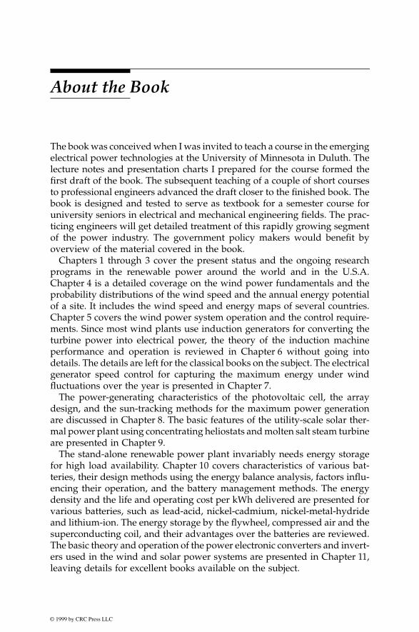
and over 90 quadrillion BTUs in the United Statesof America, distributed in segments shown in Figure 1-1. About 40 percentof the total primary energy is used in generating electricity. Nearly 70 percentof the energy used in our homes and offices is in the form of electricity. Tomeet this demand, 700 GW of electrical generating capacity is now installedin the U.S.A. For most of this century, the U.S. electric demand has increasedwith the gross national product (GNP). At that rate, the U.S. will need toinstall additional 200 GW capacity by the year 2010.
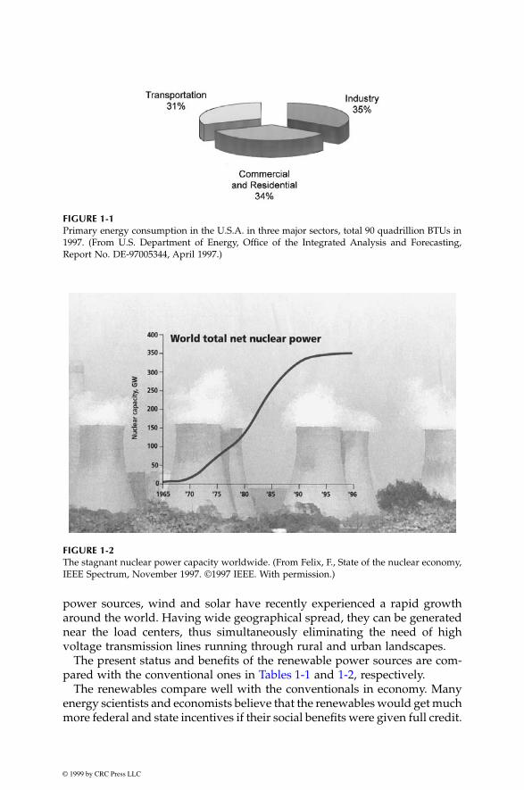
The new capacity installation decisions today are becoming complicatedin many parts of the world because of difficulty in finding sites for newgeneration and transmission facilities of any kind. In the U.S.A., no nuclearpower plants have been ordered since 1978
2
(Figure 1-2). Given the potentialfor cost overruns, safety related design changes during the construction, andlocal opposition to new plants, most utility executives suggest that none willbe ordered in the foreseeable future. Assuming that no new nuclear plantsare built, and that the existing plants are not relicensed at the expiration oftheir 40-year terms, the nuclear power output is expected to decline sharplyafter 2010. This decline must be replaced by other means. With gas pricesexpected to rise in the long run, utilities are projected to turn increasinglyto coal for base load-power generation. The U.S.A. has enormous reservesof coal, equivalent to more than 250 years of use at current level. However,that will need clean coal burning technologies that are fully acceptable tothe public.
An alternative to the nuclear and fossil fuel power is renewable energytechnologies (hydro, wind, solar, biomass, geothermal, and ocean). Large-scale hydroelectric projects have become increasingly difficult to carrythrough in recent years because of competing use of land and water. Reli-censing requirements of existing hydro plants may even lead to removal ofsome dams to protect or restore wildlife habitats. Among the other renewable
© 1999 by CRC Press LLC
power sources, wind and solar have recently experienced a rapid growtharound the world. Having wide geographical spread, they can be generatednear the load centers, thus simultaneously eliminating the need of highvoltage transmission lines running through rural and urban landscapes.
The present status and benefits of the renewable power sources are com-pared with the conventional ones in Tables 1-1 and 1-2, respectively.
The renewables compare well with the conventionals in economy. Manyenergy scientists and economists believe that the renewables would get muchmore federal and state incentives if their social benefits were given full credit.
FIGURE 1-1
Primary energy consumption in the U.S.A. in three major sectors, total 90 quadrillion BTUs in1997. (From U.S. Department of Energy, Office of the Integrated Analysis and Forecasting,Report No. DE-97005344, April 1997.)
FIGURE 1-2
The stagnant nuclear power capacity worldwide. (From Felix, F., State of the nuclear economy,IEEE Spectrum, November 1997. ©1997 IEEE. With permission.)

© 1999 by CRC Press LLC
For example, the value of not generating one ton of CO
2
, SO
2
, and NOx, andthe value of not building long high voltage transmission lines through ruraland urban areas are not adequately reflected in the present evaluation of therenewables.
1.2 Incentives for Renewables
A great deal of renewable energy development in the U.S.A. occurred in the1980s, and the prime stimulus for it was the passage in 1978 of the PublicUtility Regulatory Policies Act (PURPA). It created a class of nonutility powergenerators known as the “qualified facilities (QFs)”. The QFs were definedto be small power generators utilizing renewable energy sources and/orcogeneration systems utilizing waste energy. For the first time, PURPArequired electric utilities to interconnect with QFs and to purchase QFs’power generation at “avoided cost”, which the utility would have incurredby generating that power by itself. PURPA also exempted QFs from certain
TABLE 1-1
Status of Conventional and Renewable Power Sources
Conventional Renewables
Coal, nuclear, oil, and natural gas Wind, solar, biomass geothermal, and oceanFully matured technologies Rapidly developing technologiesNumerous tax and investment subsidies embedded in national economies
Some tax credits and grants available from some federal and/or state governments
Accepted in society under the ‘grandfather clause’ as necessary evil
Being accepted on its own merit, even with limited valuation of their environmental and other social benefits
TABLE 1-2
Benefits of Using Renewable Electricity
Traditional BenefitsNontraditional Benefits
Per Million kWh consumed
Monetary value of kWh consumedU.S. average 12 cents/kWhU.K. average 7.5 pence/kWh
Reduction in emission750–1000 tons of CO
2
7.5–10 tons of SO
2
3–5 tons of NOx50,000 kWh reduction in energy loss in power lines and equipment
Life extension of utility power distribution equipmentLower capital cost as lower capacity equipment can be used (such as transformer capacity reduction of 50 kW per MW installed)

© 1999 by CRC Press LLC
federal and state utility regulations. Furthermore, significant federal invest-ment tax credit, research and development tax credit, and energy tax credit,liberally available up to the mid 1980s, created a wind rush in California,the state that also gave liberal state tax incentives. As of now, the financialincentives in the U.S.A. are reduced, but are still available under the EnergyPolicy Act of 1992, such as the energy tax credit of 1.5 cents per kWh. Thepotential impact of the 1992 act on renewable power producers is reviewedin Chapter 16.
Globally, many countries offer incentives and guaranteed price for therenewable power. Under such incentives, the growth rate of the wind powerin Germany and India has been phenomenal.
1.3 Utility Perspective
Until the late 1980s, the interest in the renewables was confined primarilyamong private investors. However, as the considerations of fuel diversity,environmental concerns and market uncertainties are becoming importantfactors into today’s electric utility resource planning, renewable energy tech-nologies are beginning to find their place in the utility resource portfolio.Wind and solar power, in particular, have the following advantages to theelectric utilities:
• Both are highly modular in that their capacity can be increasedincrementally to match with gradual load growth.
• Their construction lead time is significantly shorter than those of theconventional plants, thus reducing the financial and regulatory risks.
• They bring diverse fuel sources that are free of cost and free of pollution.
Because of these benefits, many utilities and regulatory bodies are increas-ingly interested in acquiring hands on experience with renewable energytechnologies in order to plan effectively for the future. The above benefitsare discussed below in further details.
1.3.1 Modularity
The electricity demand in the U.S.A. grew at 6 to 7 percent until the late1970s, tapering to just 2 percent in the 1990s as shown in Figure 1-3.
The 7 percent growth rate of the 1970s meant doubling the electrical energydemand and the installed capacity every 10 years. The decline in the growthrate since then has come partly from the improved efficiency in electricityutilization through programs funded by the U.S. Department of Energy. Thesmall growth rate of the 1990s is expected to continue well into the next century.

© 1999 by CRC Press LLC
The economic size of the conventional power plant has been 500 MW to1,000 MW capacity. These sizes could be justified in the past, as the entirepower plant of that size, once built, would be fully loaded in just a few years.At a 2 percent growth rate, however, it could take decades before a 500 MWplant could be fully loaded after it is commissioned in service. Utilities areunwilling to take such long-term risks in making investment decisions. Thishas created a strong need of modularity in today’s power generation industry.
Both the wind and the solar photovoltaic power are highly modular. Theyallow installations in stages as needed without losing the economy of sizein the first installation. The photovoltaic (pv) is even more modular than thewind. It can be sized to any capacity, as the solar arrays are priced directlyby the peak generating capacity in watts, and indirectly by square foot. Thewind power is modular within the granularity of the turbine size. Standardwind turbines come in different sizes ranging from tens of kW to hundredsof kW. Prototypes of a few MW wind turbines are also tested and are beingmade commercially available in Europe. For utility scale installations, stan-dard wind turbines in the recent past have been around 300 kW, but is nowin the 500-1,000 kW range. A large plant consists of the required numberand size of wind turbines for the initially needed capacity. More towers areadded as needed in the future with no loss of economy.
For small grids, the modularity of the pv and wind systems is even moreimportant. Increasing demand may be more economically added in smallerincrements of the green power capacity. Expanding or building a new con-ventional power plant in such cases may be neither economical nor free fromthe market risk. Even when a small grid is linked by transmission line tothe main network, installing a wind or pv plant to serve growing demandmay be preferable to laying another transmission line. Local renewable
FIGURE 1-3
Growth of electricity demand in the U.S.A. (Source: U.S. Department of Energy and ElectricPower Research Institute)

© 1999 by CRC Press LLC
power plants can also benefit small power systems by moving generationnear the load, thus reducing voltage drop at the end of a long overloaded line.
In the developing countries like China and India, the demand has beenrising at a 10 percent growth rate or more. This growth rate, when viewedwith the large population base, makes these two countries rapidly growingelectrical power markets for all sources of electrical energy, including therenewables.
1.3.2 Emission-Free
In 1995, the U.S.A. produced 3 trillion kWh of electricity, 70 percent of it(2 trillion kWh) from fossil fuels, a majority of that came from coal. Theresulting emission is estimated to be 2 billion tons of CO
2
, 15 million tons ofSO
2
and 6 million tons of NOx. The health effects of these emissions are ofsignificant concern to the U.S. public. The electromagnetic field emissionaround the high voltage transmission lines is another concern that has alsorecently become an environmental issue.
For these benefits, the renewable energy sources are expected to findimportance in the energy planning in all countries around the world.
References
1. U.S. Department of Energy. 1997. “International Energy Outlook 1997 withProjections to 2015,”
DOE Office of the Integrated Analysis and Forecasting, ReportNo. DE-97005344,
April 1997.2. Felix, F. 1992. “State of the Nuclear Economy,”
IEEE Spectrum,
November 1997,p. 29-32.

© 1999 by CRC Press LLC
2
Wind Power
The first use of wind power was to sail ships in the Nile some 5000 yearsago. The Europeans used it to grind grains and pump water in the 1700sand 1800s. The first windmill to generate electricity in the rural U.S.A. wasinstalled in 1890. Today, large wind-power plants are competing with electricutilities in supplying economical clean power in many parts of the world.
The average turbine size of the wind installations has been 300 kW untilthe recent past. The newer machines of 500 to 1,000 kW capacity have beendeveloped and are being installed. Prototypes of a few MW wind turbinesare under test operations in several countries, including the U.S.A. Figure 2-1is a conceptual layout of modern multimegawatt wind tower suitable forutility scale applications.
1
Improved turbine designs and plant utilization have contributed to adecline in large-scale wind energy generation costs from 35 cents per kWhin 1980 to less than 5 cents per kWh in 1997 in favorable locations(Figure 2-2). At this price, wind energy has become one of the least-costpower sources. Major factors that have accelerated the wind-power technol-ogy development are as follows:
• high-strength fiber composites for constructing large low-cost blades.• falling prices of the power electronics.• variable-speed operation of electrical generators to capture maxi-
mum energy.• improved plant operation, pushing the availability up to 95 percent.• economy of scale, as the turbines and plants are getting larger in size.• accumulated field experience (the learning curve effect) improving
the capacity factor.
2.1 Wind in the World
The wind energy stands out to be one of the most promising new sourcesof electrical power in the near term. Many countries promote the wind-power

© 1999 by CRC Press LLC
FIGURE 2-1
Modern wind turbine for utility scale power generation.

© 1999 by CRC Press LLC
technology by national programs and market incentives. The InternationalEnergy Agency (IEA), with funding from 14 countries, supports jointresearch projects and information exchange on wind-power development.
2
These countries are Austria, Canada, Denmark, Finland, Germany, Italy,Japan, the Netherlands, New Zealand, Norway, Spain, Sweden, the UnitedKingdom, and the United States of America. By the beginning of 1995, morethan 25,000 grid-connected wind turbines were operating in the IEA-membercountries, amounting to a rated power capacity of about 3,500 MW. Collec-tively, these turbines are producing more than 6 million MWh of energyevery year. The annual rate of capacity increase presently is about 600 MW.
According to the AWEA and the IEA, the 1994, 1995, and 1997 installedcapacity in countries listed in Table 2-1 were 3,552 MW, 4,776 MW, and7,308 MW, respectively. The 1995 sales of new plants set a record of 1224 MW($1.5 billion), boosting the global installed capacity by 35 percent to nearly4,776 MW. The most explosive growth occurred in Germany installing500 MW and India adding 383 MW to their wind capacities. New wind plantsinstalled in 1996-97 added another 2,532 MW to that total with an annualgrowth rate of 24 percent.
Much of the new development around the world can be attributed togovernment policies to promote the renewables energy sources. For example,the United Kingdom’s nonfossil fuel obligation program will add 500 MWof wind power to the UK’s power grid within this decade.
A 1994 study, commissioned by the American Wind Energy Association(AWEA) with Arthur D. Little Inc., concluded that in the 10 overseas windfarm markets, between 1,935 MW and 3,525 MW of wind capacity would beadded by the year 2000 (Table 2-2). This translates to between $2 to$3.5 billion in sales.
FIGURE 2-2
Declining cost of wind-generated electricity. (Source: AWEA/DOE/IEA.)

© 1999 by CRC Press LLC
2.2 The U.S.A.
Large-scale wind-power development in the U.S.A. has been going on sincethe late 1970s. In 1979, a 2 MW experimental machine was installed jointlyby the Department of Energy and NASA on the Howard Knob Mountainnear Boone, North Carolina. The system was designed and built by the
TABLE 2-1
Installed Wind Capacity in Selected Countries, 1994, 1995 and 1997
Country1994MW
1995MW
1997MW
Growth1994-1995Percent
Annual Growth Rate1995-97Percent
Germany 643 1136 2079 76.7 35.2United States 1785 1828 2000 2.4 4.7Denmark 540 614 1141 13.7 36.3India 182 565 1000 210 33.0Netherlands 153 259 325 69 12.0United Kingdom 147 193 308 31 26.3Spain 72 145 455 100 77.1China 30 36 — 20 —TOTAL 3552 4776 7308 35.4 23.7
(Source: United States data from Energy Information Administration, Annual EnergyOutlook 1997, DOE/EIA Report No. 0383-97, Table A17, Washington, D.C., December1996. Other countries data from the Amercian Wind Energy Association, Satus Reportof International Wind Projects, Washington, D.C., March 1996.)
TABLE 2-2
Projected Wind Capacity Addition in
Megawatts Between 1994 and 2000
CountryAddition planned
Megawatts
United Kingdom 100–300Spain 150–250Germany 200–350India 700–1200China 350–600Mexico 150–300Argentina 100–150Chile 100–200Australia 50–75New Zealand 50–100Total 1950–3525
(Source: American Wind Energy Associa-tion/Arthur D. Little, Inc.)
© 1999 by CRC Press LLC
General Electric Company using two 61-meter diameter rotor blades fromBoeing Aerospace Corporation. It was connected to the local utility grid andoperated successfully.
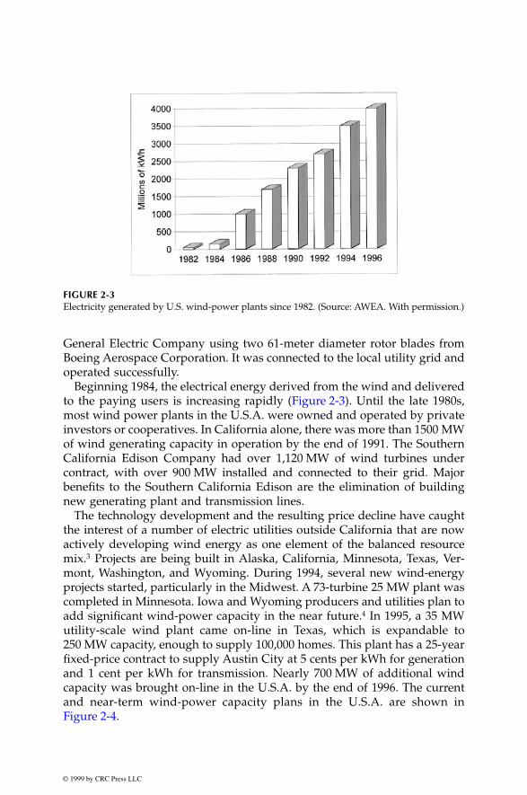
Beginning 1984, the electrical energy derived from the wind and deliveredto the paying users is increasing rapidly (Figure 2-3). Until the late 1980s,most wind power plants in the U.S.A. were owned and operated by privateinvestors or cooperatives. In California alone, there was more than 1500 MWof wind generating capacity in operation by the end of 1991. The SouthernCalifornia Edison Company had over 1,120 MW of wind turbines undercontract, with over 900 MW installed and connected to their grid. Majorbenefits to the Southern California Edison are the elimination of buildingnew generating plant and transmission lines.
The technology development and the resulting price decline have caughtthe interest of a number of electric utilities outside California that are nowactively developing wind energy as one element of the balanced resourcemix.
3
Projects are being built in Alaska, California, Minnesota, Texas, Ver-mont, Washington, and Wyoming. During 1994, several new wind-energyprojects started, particularly in the Midwest. A 73-turbine 25 MW plant wascompleted in Minnesota. Iowa and Wyoming producers and utilities plan toadd significant wind-power capacity in the near future.
4
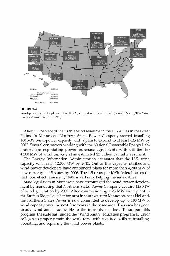
In 1995, a 35 MWutility-scale wind plant came on-line in Texas, which is expandable to250 MW capacity, enough to supply 100,000 homes. This plant has a 25-yearfixed-price contract to supply Austin City at 5 cents per kWh for generationand 1 cent per kWh for transmission. Nearly 700 MW of additional windcapacity was brought on-line in the U.S.A. by the end of 1996. The currentand near-term wind-power capacity plans in the U.S.A. are shown inFigure 2-4.
FIGURE 2-3
Electricity generated by U.S. wind-power plants since 1982. (Source: AWEA. With permission.)
© 1999 by CRC Press LLC
About 90 percent of the usable wind resource in the U.S.A. lies in the GreatPlains. In Minnesota, Northern States Power Company started installing100 MW wind-power capacity with a plan to expand to at least 425 MW by2002. Several contractors working with the National Renewable Energy Lab-oratory are negotiating power purchase agreements with utilities for4,200 MW of wind capacity at an estimated $2 billion capital investment.
The Energy Information Administration estimates that the U.S. windcapacity will reach 12,000 MW by 2015. Out of this capacity, utilities andwind-power developers have announced plans for more than 4,200 MW ofnew capacity in 15 states by 2006. The 1.5 cents per kWh federal tax creditthat took effect January 1, 1994, is certainly helping the renewables.
State legislators in Minnesota have encouraged the wind power develop-ment by mandating that Northern States Power Company acquire 425 MWof wind generation by 2002. After commissioning a 25 MW wind plant inthe Buffalo Ridge Lake Benton area in southwestern Minnesota near Holland,the Northern States Power is now committed to develop up to 100 MW ofwind capacity over the next few years in the same area. This area has goodsteady wind and is accessible to the transmission lines. To support thisprogram, the state has funded the “Wind Smith” education program at juniorcolleges to properly train the work force with required skills in installing,operating, and repairing the wind power plants.
FIGURE 2-4
Wind-power capacity plans in the U.S.A., current and near future. (Source: NREL/IEA WindEnergy Annual Report, 1995.)

© 1999 by CRC Press LLC
2.3 Europe
The wind-power picture in Europe is rapidly growing. The 1995 projectionson the expected wind capacity in 2000 have been met in 1997, in approximatelyone-half of the time. Figure 2-5 depicts the wind capacity installed in theEuropean countries at the end of 1997. The total capacity installed was4,694 MW. The new targets adopted by the European Wind Energy Associationare 40,000 MW capacity by 2010 and 100,000 MW by 2020. These targets formpart of a series of policy objectives agreed by the association in November
FIGURE 2-5
Installed wind capacity in European countries as of December 1997. (Source: Wind Directions,Magazine of the European Wind Energy Association, London, January 1998. With permission.)

© 1999 by CRC Press LLC
1997. Germany and Denmark lead Europe in the wind power. Both haveachieved phenomenal growth through guaranteed tariff based on the domes-tic electricity prices. Germany has a 35-fold increase between 1990 and 1996.With 2,079 MW installed capacity, Germany is now the world leader. Theformer global leader, the U.S.A., has seen only a small increase during thisperiod, from 1,500 MW in 1990 to approximately 2,000 MW in 1997.
2.4 India
India has 9 million square kilometers land area with a population over900 million, of which 75 percent live in agrarian rural areas. The total powergenerating capacity has grown from 1,300 MW in 1950 to about 100,000 MWin 1998 at an annual growth rate of about nine percent. At this rate, Indianeeds to add 10,000 MW capacity every year. The electricity network reachesover 500,000 villages and powers 11 million agricultural water-pumpingstations. Coal is the primary source of energy. However, coal mines areconcentrated in certain areas, and transporting coal to other parts of thecountry is not easy. One-third of the total electricity is used in the rural areas,where three-fourths of the population lives. The transmission and distribu-tion loss in the electrical network is relatively high at 25 percent. The envi-ronment in a heavily-populated area is more of a concern in India than inother countries. For these reasons, the distributed power system, such aswind plants near the load centers, are of great interest to the state-ownedelectricity boards. The country has adopted aggressive plans for developingthese renewables. As a result, India today has the largest growth rate of thewind capacity and is one of the largest producers of wind energy in theworld.
5
In 1995, it had 565 MW of wind capacity, and some 1,800 MWadditional capacity is in various stages of planning. The government hasidentified 77 sites for economically feasible wind-power generation, with agenerating capacity of 4,000 MW of grid-quality power.
It is estimated that India has about 20,000 MW of wind power potential,out of which 1,000 MW has been installed as of 1997. With this, India nowranks in the first five countries in the world in wind-power generation, andprovides attractive incentives to local and foreign investors. The Tata EnergyResearch Institute’s office in Washington, D.C., provides a link between theinvestors in India and in the U.S.A.
2.5 Mexico
Mexico has over a decade of experience with renewable power systems. Thetwo federally-owned utilities provide power to 95 percent of Mexico’s

© 1999 by CRC Press LLC
population. However, there are still 90,000 hard-to-access villages with fewerthan 1,000 inhabitants without electricity. These villages are being poweredby renewable systems with deep cycle lead-acid batteries for energy storage.The wind resource has been thoroughly mapped in collaboration with theU.S. National Renewable Energy Laboratory.
6
2.6 Ongoing Research and Development
The total government research and development funding in the InternationalEnergy Agency member countries in 1995 was about $200 million. The U.S.Department of Energy funded about $50 million worth of research and devel-opment in 1995. The goal of these programs is to further reduce the windelectricity-generation cost to less than 4 cents per kWh by the year 2000. TheDepartment of Energy and the U.S. national laboratories also have a numberof programs to promote the wind-hybrid power technologies throughoutthe developing world, with particular emphasis on Latin America and thePacific Rim countries.
7
These activities include feasibility studies and pilotprojects, project financing and supporting renewable energy educationefforts.
References
1. U.S. Department of Energy. 1995. “Wind Energy Programs Overview,”
NRELReport No. DE-95000288,
March 1995.2. International Energy Agency. 1995. “Wind Energy Annual Report,”
InternationalEnergy Agency Report by NREL,
March 1995.3. Utility Wind Interest Group. 1995. “Utilities Move Wind Technology Across
America,”
1995 Report.
November 1995.4. Anson, S., Sinclair, K., and Swezey, B. 1994. “Profiles in Renewables Energy,”
Case studies of successful utility-sector projects, DOE/NREL Report No. DE-930000081,
National Renewable Energy Laboratory, Golden, Colorado, August1994.
5. Gupta, A. K. 1997. “Power Generation from Renewables in India,”
Ministry ofNon-Conventional Energy Sources,
New Delhi, India, 1997.6. Schwartz, M. N. and Elliott, D. L. 1995. “Mexico’s Wind Resources Assessment
Project,”
DOE/NREL Report No. DE-AC36-83CH10093,
National Renewable En-ergy Laboratory, Golden, Colorado, May 1995.
7. Hammons, T. J., Ramakumar, R., Fraser, M., Conners, S. R., Davies, M., Holt,E. A., Ellis, M., Boyers, J., and Markard, J. 1997. “Renewable Energy TechnologyAlternatives for Developing Countries,”
IEEE Power Engineering Review,
De-cember 1997, p. 10-21.

© 1999 by CRC Press LLC
3
Photovoltaic Power
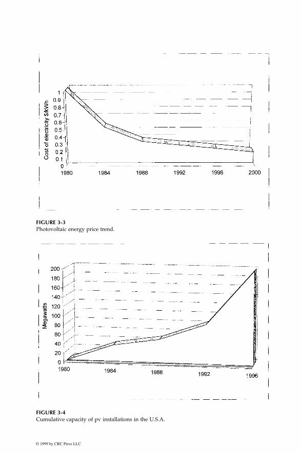
The photovoltaic (pv) power technology uses semiconductor cells (wafers),generally several square centimeters in size. From the solid-state physicspoint of view, the cell is basically a large area p-n diode with the junctionpositioned close to the top surface. The cell converts the sunlight into directcurrent electricity. Numerous cells are assembled in a module to generaterequired power (Figure 3-1). Unlike the dynamic wind turbine, the pv instal-lation is static, does not need strong tall towers, produces no vibration ornoise, and needs no cooling. Because much of the current pv technologyuses crystalline semiconductor material similar to integrated circuit chips,the production costs have been high. However, between 1980 and 1996, thecapital cost of pv modules per watt of power capacity has declined frommore than $20 per watt to less than $5 per watts (Figure 3-2). During thesame period, the cost of pv electricity has declined from almost $1 to about$0.20 per kWh, and is expected to decline to $0.15 per kWh by the year 2000(Figure 3-3). The installed capacity in the U.S. has risen from nearly zero in1980 to approximately 200 MW in 1996 (Figure 3-4). The world capacity ofpv systems was about 350 MW in 1996, which could increase to almost1,000 MW by the end of this century (Figure 3-5).
The pv cell manufacturing process is energy intensive. Every square cen-timeter cell area consumes a few kWh before it faces the sun and producesthe first kWh of energy. However, the manufacturing energy consumptionis steadily declining with continuous implementation of new productionprocesses (Figure 3-6).
The present pv energy cost is still higher than the price the utility custom-ers pay in most countries. For that reason, the pv applications have beenlimited to remote locations not connected to the utility lines. With the declin-ing prices, the market of new modules has been growing at more than a15 percent annual rate during the last five years. The United States, theUnited Kingdom, Japan, China, India, and other countries have establishednew programs or have expanded the existing ones. It has been estimatedthat the potential pv market, with new programs coming in, could be asgreat as 1,600 MW by 2010. This is a significant growth projection, largelyattributed to new manufacturing plants installed in the late 1990s to manu-facture low cost pv cells and modules to meet the growing demand.

© 1999 by CRC Press LLC
Major advantages of the photovoltaic power are as follows:
• short lead time to design, install, and start up a new plant.• highly modular, hence, the plant economy is not a strong function
of size.• power output matches very well with peak load demands.• static structure, no moving parts, hence, no noise.• high power capability per unit of weight.• longer life with little maintenance because of no moving parts.• highly mobile and portable because of light weight.
Almost 40 percent of the pv modules installed in the world are producedin the United States of America. Approximately 40 MW modules were pro-duced in the U.S.A. in 1995, out of which 19 MW were produced by SiemensSolar Industries and 9.5 MW by Solarex Corporation.
FIGURE 3-1
Photovoltaic module in sunlight generates direct current electricity. (Source: Solarex Corpora-tion, Frederick, Md. With permission.)

© 1999 by CRC Press LLC
3.1 Present Status
At present, pv power is extensively used in stand-alone power systems inremote villages, particularly in hybrid with diesel power generators. It isexpected that this application will continue to find expanding markets inmany countries. The driving force is the energy need in developing countries,and the environmental concern in developed countries. In the United States,city planners are recognizing the favorable overall economics of the pvpower for urban applications. Tens of thousands of private, federal, stateand commercial pv systems have been installed over the last 20 years. Morethan 65 cities in 24 states have installed such systems for a variety of neededservices. These cities, shown in Figure 3-7, are located in all regions of thecountry, dispensing the myth that pv systems require a sunbelt climate towork effectively and efficiently.
The U.S. utilities have started programs to develop power plants using thenewly available low-cost pv modules. Idaho Power has a pilot program tosupply power to selected customers not yet connected to the grid. Other
FIGURE 3-2
Photovoltaic module price trend.
© 1999 by CRC Press LLC
FIGURE 3-3
Photovoltaic energy price trend.
FIGURE 3-4
Cumulative capacity of pv installations in the U.S.A.

© 1999 by CRC Press LLC
utilities such as Southern California Edison, the municipal utility of Austin,Delmarva Power and Light, and New York Power Authority are installingsuch systems to meet peak demands. The Pacific Gas and Electric’s utility-scale 500 kW plant at Kerman is designed to deliver power during the localpeak demand. It generates 1.1 MWh of energy annually.
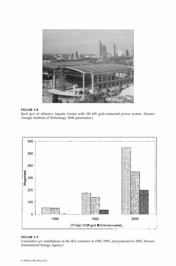
The roof of the Aquatic Center in Atlanta (Figure 3-8), venue of the 1996Olympic swimming competition, is one of the largest grid-connected powerplants. It generates 345 kW of electric power, and is tied into the GeorgiaPower grid lines. Its capacity is enough to power 70 homes connected to thenetwork. It saves 330 tons of CO
2
, 3.3 tons of SO
2
and 1.2 tons of NOx yearly.Installations are under way to install a similar 500 kW grid-connected pvsystem to power the Olympics Games of 2000 in Sydney, Australia.
In 14 member countries of the International Energy Agency, the pv installa-tions are being added at an average annual growth rate of 27 percent. Thetotal installed capacity increased from 54 MW in 1990 to 176 MW in 1995. TheIEA estimates that by the end of 2000, 550 MW of additional capacity will beinstalled, 64 percent off-grid and 36 percent grid-connected (Figure 3-9).
India is implementing perhaps the most number of pv systems in the worldfor remote villages. About 30 MW capacity has already been installed, withmore being added every year. The country has a total production capacityof 8.5 MW modules per year. The remaining need is met by imports. A
FIGURE 3-5
Cumulative capacity of pv installations in the world.

© 1999 by CRC Press LLC
FIGURE 3-6
Energy consumption per cm
2
of pv cell manufactured. (Source: U.S. Department of Commerceand Dataquest, Inc.)
FIGURE 3-7
U.S. cities with pv installations. (Source: Department of Energy, 1995.)
© 1999 by CRC Press LLC
FIGURE 3-8
Roof (pv) of Atlanta’s Aquatic Center with 345 kW grid-connected power system. (Source:Georgia Institute of Technology. With permission.)
FIGURE 3-9
Cumulative pv installations in the IEA countries in 1990, 1995, and projected to 2000. (Source:International Energy Agency.)

© 1999 by CRC Press LLC
700 kW grid-connected pv plant has been commissioned, and a 425 kWcapacity is under installation in Madhya Pradesh. The state of West Bengalhas decided to convert the Sagar Island into a pv island. The island has150,000 inhabitants in 16 villages spread out in an area of about 300 squarekilometers. The main source of electricity at present is diesel, which is expen-sive and is causing severe environmental problems on the island.
The state of Rajasthan has initialed a policy to purchase pv electricity atan attractive rate of $0.08 per kWh. In response, a consortium of Enron andAmoco has proposed installing a 50 MW plant using thin film cells. Whencompleted, this will be the largest pv power plant in the world.
The studies at the Arid Zone Research Institute, Jodhpur, indicate signifi-cant solar energy reaching the earth surface in India. About 30 percent ofthe electrical energy used in India is for agricultural needs. Since the avail-ability of solar power for agricultural need is not time critical (within a fewdays), India is expected to lead the world in pv installations in near future.
3.2 Building Integrated pv Systems
In new markets, the near-term potentially large application of the pv tech-nology is for cladding buildings to power air-conditioning and lightingloads. One of the attractive features of the pv system is that its power outputmatches very well with the peak load demand. It produces more power ona sunny summer day when the air-conditioning load strains the grid lines(Figure 3-10). The use of pv installations in buildings has risen from a mere3 MW in 1984 to 16 MW in 1994, at a rate of 18 percent per year.
In the mid 1990s, the DOE launched a 5-year cost-sharing program withSolarex Corporation of Maryland to develop and manufacture low cost, easyto install, pre-engineered Building Integrated Photovoltaic (BIPV) modules.Such modules made in shingles and panels can replace traditional roofs andwalls. The building owners have to pay only the incremental cost of thesecomponents. The land is paid for, the support structure is already in there,the building is already wired, and developers may finance the BIPV as partof their overall project. The major advantage of the BIPV system is that itproduces power at the point of consumption. The BIPV, therefore, offers thefirst potentially widespread commercial implementation of the pv technol-ogy in the industrialized countries. The existing programs in the U.S.A.,Europe, and Japan could add 200 MW of BIPV installations by the year 2010.Worldwide, the Netherlands plans to install 250 MW by 2010, and Japan hasplans to add 185 MW between 1993 and 2000.
Figure 3-11 shows a building-integrated and grid-connected pv power sys-tem recently installed and operating in Germany.
In August 1997, The DOE announced that it will lead an effort to placeone million solar-power systems on home and building roofs across the

© 1999 by CRC Press LLC
U.S.A. by the year 2010. This “Million Solar Roof Initiative” is expected toincrease the momentum for more widespread use of solar power, loweringthe cost of photovoltaic technologies.
FIGURE 3-10
Power usage in commercial building on a typical summer day.
FIGURE 3-11
Building-integrated pv systems in Germany. (Source: Professional Engineering, Publication ofthe Institution of Mechanical Engineers, April 1997, U.K.. With permission.)

© 1999 by CRC Press LLC
3.3 pv Cell Technologies
In making comparisons between alternative power technologies, the mostimportant measure is the energy cost per kWh delivered. In pv power, thiscost primarily depends on two parameters, the photovoltaic energy conver-sion efficiency, and the capital cost per watt capacity. Together, these twoparameters indicate the economic competitiveness of the pv electricity.
The conversion efficiency of the photovoltaic cell is defined as follows:
The continuing development efforts to produce more efficient low costcells have resulted in various types of pv technologies available in the markettoday, in terms of the conversion efficiency and the module cost. The majortypes are discussed in the following sections:
1
3.3.1 Single-Crystalline Silicon
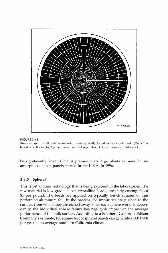
The single crystal silicon is the widely available cell material, and has beenthe workhorse of the industry. In the most common method of producingthis material, the silicon raw material is first melted and purified in a crucible.A seed crystal is then placed in the liquid silicon and drawn at a slow constantrate. This results in a solid, single-crystal cylindrical ingot (Figure 3-12). Themanufacturing process is slow and energy intensive, resulting in high rawmaterial cost presently at $25 to $30 per pound. The ingot is sliced using adiamond saw into 200 to 400 µm (0.005 to 0.010 inch) thick wafers. The wafersare further cut into rectangular cells to maximize the number of cells that canbe mounted together on a rectangular panel. Unfortunately, almost half ofthe expensive silicon ingot is wasted in slicing ingot and forming square cells.The material waste can be minimized by making the full size round cellsfrom round ingots (Figure 3-13). Using such cells would be economical wherethe panel space is not at a premium. Another way to minimize the waste isto grow crystals on ribbons. Some U.S. companies have set up plants to drawpv ribbons, which are then cut by laser to reduce waste.
3.3.2 Polycrystalline and Semicrystalline
This is relatively a fast and low cost process to manufacture thick crystallinecells. Instead of drawing single crystals using seeds, the molten silicon iscast into ingots. In the process, it forms multiple crystals. The conversionefficiency is lower, but the cost is much lower, giving a net reduction in costper watt of power.
η = electrical power outputsolar power impinging the cell

© 1999 by CRC Press LLC
3.3.3 Thin Films
These are new types of photovoltaics entering the market. Copper IndiumDiselenide, Cadmium Telluride, and Gallium Arsenide are all thin film mate-rials, typically a few µm or less in thickness, directly deposited on glass,stainless steel, ceramic or other compatible substrate materials. This technol-ogy uses much less material per square area of the cell, hence, is less expen-sive per watt of power generated.
3.3.4 Amorphous Silicon
In this technology, amorphous silicon vapor is deposited on a couple of µm-thick amorphous (glassy) films on stainless steel rolls, typically 2,000-feetlong and 13-inches wide. Compared to the crystalline silicon, this technologyuses only 1 percent of the material. Its efficiency is about one-half of thecrystalline silicon at present, but the cost per watt generated is projected to
FIGURE 3-12
Single-crystal ingot-making by Czochralski process. (Source: Cook, G., Photovoltaic Fundamen-tal, DOE/NREL Report DE91015001, February 1995.)
© 1999 by CRC Press LLC
be significantly lower. On this premise, two large plants to manufactureamorphous silicon panels started in the U.S.A. in 1996.
3.3.5 Spheral
This is yet another technology that is being explored in the laboratories. Theraw material is low-grade silicon crystalline beads, presently costing about$1 per pound. The beads are applied on typically 4-inch squares of thinperforated aluminum foil. In the process, the impurities are pushed to thesurface, from where they are etched away. Since each sphere works indepen-dently, the individual sphere failure has negligible impact on the averageperformance of the bulk surface. According to a Southern California EdisonCompany’s estimate, 100 square feet of spheral panels can generate 2,000 kWhper year in an average southern California climate.
FIGURE 3-13
Round-shape pv cell reduces material waste typically found in rectangular cell. (Depictionbased on cell used by Applied Solar Energy Corporation, City of Industry, California.)

© 1999 by CRC Press LLC
3.3.6 Concentrated Cells
In an attempt to improve the conversion efficiency, the sunlight is concen-trated into tens or hundreds of times the normal sun intensity by focusingon a small area using low cost lenses (Figure 3-14). The primary advantageis that such cells require a small fraction of area compared to the standardcells, thus significantly reducing the pv material requirement. However, thetotal module area remains the same to collect the required sun power. Besidesincreasing the power and reducing the size or number of cells, such cellshave additional advantage that the cell efficiency increases under concen-trated light up to a point. Another advantage is that they can use small areacells. It is easier to produce high efficiency cells of small areas than to producelarge area cells with comparable efficiency. On the other hand, the majordisadvantage of the concentrator cells is that they require focusing opticsadding into the cost.
The annual production of various pv cells in 1995 is shown in Table 3-1.Almost all production has been in the crystalline silicon and the amorphoussilicon cells, with other types being in the development stage. The presentstatus of the crystalline silicon and the amorphous silicon technologies isshown in Table 3-2. The former is dominant in the market at present and thelatter is expected to be dominant in the near future.
FIGURE 3-14
Lens concentrating the sunlight on small area reduces the need of active cell material. (Source:Photovoltaic Fundamental, DOE/NREL Report DE91015001, February 1995.)

© 1999 by CRC Press LLC
3.4 pv Energy Maps
The solar energy impinging the surface of the earth is depicted in Figure 3-15,where the white areas get more solar radiation per year. The yearly 24-houraverage solar flux reaching the horizontal surface of the earth is shown inFigure 3-16, whereas Figure 3-17 depicts that in the month of December. Noticethat the 24-hour average decreases in December. This is due to the shorter daysand clouds, and not due to the cold temperature. As will be seen later, the pvcell actually converts more solar energy into electricity at low temperatures.
It is the total yearly energy capture potential of the site that determinesthe economical viability of installing a power plant. Figure 3-18 is useful inthis regard, as it gives the annual average solar energy per day impingingon the surface always facing the sun at right angle. Modules mounted on asun-tracking structure receive this energy. The electric energy produced perday is obtained by multiplying the map number by the photoconversionefficiency of the modules installed at the site.
TABLE 3-1
Production Capacities of Various pv Technologies
in 1995
PV Technology 1995 Production
Crystalline Silicon 55 MWAmorphous Silicon 9 MWRibbon Si, GaAs, CdTe 1 MWTOTAL 65 MW
(Source: Carlson, D. E., Recent Advances in Photovoltaics,1995. Proceedings of the Intersociety Engineering Confer-ence on Energy Conversion, 1995.)
TABLE 3-2
Comparison of Crystalline and Amorphous Silicon Technologies
Crystalline Silicon Amorphous Silicon
Present Status Workhorse of terrestrial and space applications
New rapidly developing technology, tens of MW yearly production facilities have been built in 1996 to produce low cost cells
Thickness 200-400 µm (.004-.008 inch) 2 µm (less then 1 percent of that in crystalline silicon)
Raw Material Cost High About 3 percent of that in crystalline siliconConversion Efficiency
16-18 percent 8-9 percent
Module Costs (1995)
$6–8 per watt, expected to fall slowly due to the matured nature of this technology
$6-8 per watt, expected to fall rapidly to $2 per watt in 2000 due to heavy DOE funding to fully develop this new technology

© 1999 by CRC Press LLC
FIGURE 3-15
Solar radiation by regions of the world (higher energy potential in the white areas).
FIGURE 3-16
Yearly 24-hour average solar radiation in watts/m
2
reaching the horizontal surface of the earth.(Source: Profiles in Renewable Energy, DOE/NREL Report No. DE-930000081, August 1994.)

© 1999 by CRC Press LLC
FIGURE 3-17
December 24-hour average solar radiation in watts/m
2
reaching the horizontal surface of theearth. (Source: Profiles in Renewable Energy, DOE/NREL Report No. DE-930000081, August1994.)
FIGURE 3-18
Yearly 24-hour average solar energy in kWh/m
2
reaching surface always facing the sun at rightangel. (Source: A. Anson, Profiles in Renewable Energy, DOE/NREL Report No. DE-930000081,August 1994.)

© 1999 by CRC Press LLC
References
1. Carlson, D. E. 1995. “Recent Advances in Photovoltaics,”
1995 Proceedings ofthe Intersociety Engineering Conference on Energy Conversion.
1995, p. 621-626.

© 1999 by CRC Press LLC
4
Wind Speed and Energy Distributions
The wind turbine captures the wind’s kinetic energy in a rotor consisting oftwo or more blades mechanically coupled to an electrical generator. Theturbine is mounted on a tall tower to enhance the energy capture. Numerouswind turbines are installed at one site to build a wind farm of the desiredpower production capacity. Obviously, sites with steady high wind producemore energy over the year.
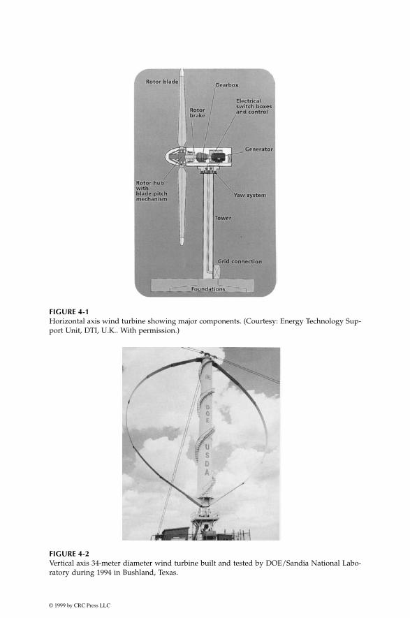
Two distinctly different configurations are available for the turbine design,the horizontal axis configuration (Figure 4-1) and the vertical axis configura-tion (Figure 4-2). The vertical axis machine has the shape of an egg beater,and is often called the Darrieus rotor after its inventor. It has been used inthe past because of specific structural advantage. However, most modernwind turbines use horizontal-axis design. Except for the rotor, all other com-ponents are the same in both designs, with some difference in their placement.
4.1 Speed and Power Relations
The kinetic energy in air of mass “m” moving with speed V is given by thefollowing in SI units:
(4-1)
The power in moving air is the flow rate of kinetic energy per second.Therefore:
(4-2)
If we let P = mechanical power in the moving air
ρ
= air density, kg/m
3
A = area swept by the rotor blades, m
2
V = velocity of the air, m/s
Kinetic Energy m V= ⋅ ⋅12
2 joules.
Power mass flow rate per V= ⋅ ( ) ⋅12
2second
© 1999 by CRC Press LLC
FIGURE 4-1
Horizontal axis wind turbine showing major components. (Courtesy: Energy Technology Sup-port Unit, DTI, U.K.. With permission.)
FIGURE 4-2
Vertical axis 34-meter diameter wind turbine built and tested by DOE/Sandia National Labo-ratory during 1994 in Bushland, Texas.

© 1999 by CRC Press LLC
then, the volumetric flow rate is A·V, the mass flow rate of the air in kilogramsper second is
ρ
·A·V, and the power is given by the following:
(4-3)
Two potential wind sites are compared in terms of the specific wind powerexpressed in watts per square meter of area swept by the rotating blades. Itis also referred to as the power density of the site, and is given by thefollowing expression:
(4-4)
This is the power in the upstream wind. It varies linearly with the densityof the air sweeping the blades, and with the cube of the wind speed. All ofthe upstream wind power cannot be extracted by the blades, as some poweris left in the downstream air which continues to move with reduced speed.
4.2 Power Extracted from the Wind
The actual power extracted by the rotor blades is the difference between theupstream and the downstream wind powers. That is, using Equation 4-2:
(4-5)
where P
o
= mechanical power extracted by the rotor, i.e., the turbine outputpower
V = upstream wind velocity at the entrance of the rotor bladesV
o
= downstream wind velocity at the exit of the rotor blades.
The air velocity is discontinuous from V to V
o
at the “plane” of the rotorblades in the macroscopic sense (we leave the aerodynamics of the bladesfor many excellent books available on the subjects). The mass flow rate ofair through the rotating blades is, therefore, derived by multiplying thedensity with the average velocity. That is:
(4-6)
P AV V AV watts= ( ) ⋅ =12
12
2 3ρ ρ .
Specific Power of the site watts per m of the rotor swept area.2= ⋅12
3ρ V
P V Vo o= ⋅ −{ }12
2 2 mass flow rate per second
mass flow rate = ⋅ ⋅+
ρ AV Vo
2

© 1999 by CRC Press LLC
The mechanical power extracted by the rotor, which is driving the electricalgenerator, is therefore:
(4-7)
The above expression can be algebraically rearranged:
(4-8)
The power extracted by the blades is customarily expressed as a fractionof the upstream wind power as follows:
(4-9)
where (4-10)
The C
p
is the fraction of the upstream wind power, which is captured bythe rotor blades. The remaining power is discharged or wasted in the down-stream wind. The factor C
p
is called the power coefficient of the rotor or therotor efficiency.
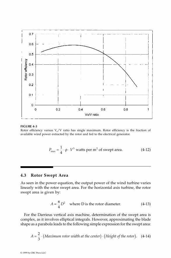
For a given upstream wind speed, the value of C
p
depends on the ratio ofthe down stream to the upstream wind speeds, that is (V
o
/V). The plot ofpower coefficient versus (V
o
/V) shows that C
p
is a single, maximum-valuefunction (Figure 4-3). It has the maximum value of 0.59 when the (V
o
/V) isone-third. The maximum power is extracted from the wind at that speedratio, when the downstream wind speed equals one-third of the upstreamspeed. Under this condition:
(4-11)
The theoretical maximum value of C
p
is 0.59. In practical designs, the max-imum achievable C
p
is below 0.5 for high-speed, two-blade turbines, andbetween 0.2 and 0.4 for slow speed turbines with more blades (Figure 4-4).If we take 0.5 as the practical maximum rotor efficiency, the maximum poweroutput of the wind turbine becomes a simple expression:
P AV V
V Voo
o= ⋅ ⋅+( )
⋅ −( )12 2
2 2ρ
P A V
VV
VV
o
o o
= ⋅ ⋅+
−
1
2
1 1
23
2
ρ
P A V Co p= ⋅ ⋅ ⋅12
3ρ
C
VV
VV
p
o o
=+
−
1 1
2
2
P A Vmax .= ⋅ ⋅ ⋅12
0 593ρ
© 1999 by CRC Press LLC
(4-12)
4.3 Rotor Swept Area
As seen in the power equation, the output power of the wind turbine varieslinearly with the rotor swept area. For the horizontal axis turbine, the rotorswept area is given by:
(4-13)
For the Darrieus vertical axis machine, determination of the swept
area iscomplex, as it involves elliptical integrals. However, approximating the bladeshape as a parabola leads to the following simple expression for the swept area:
(4-14)
FIGURE 4-3
Rotor efficiency versus V
o
/V ratio has single maximum. Rotor efficiency is the fraction ofavailable wind power extracted by the rotor and fed to the electrical generator.
P Vmax = ⋅ ⋅14
3ρ watts per m of swept area.2
A D= π4
2 where D is the rotor diameter.
A = ⋅ ( ) ⋅ ( )23
Maximum rotor width at the center Height of the rotor .
© 1999 by CRC Press LLC
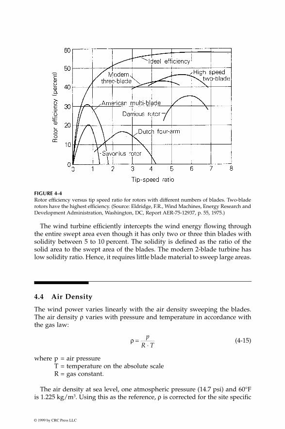
The wind turbine efficiently intercepts the wind energy flowing throughthe entire swept area even though it has only two or three thin blades withsolidity between 5 to 10 percent. The solidity is defined as the ratio of thesolid area to the swept area of the blades. The modern 2-blade turbine haslow solidity ratio. Hence, it requires little blade material to sweep large areas.
4.4 Air Density
The wind power varies linearly with the air density sweeping the blades.The air density
ρ
varies with pressure and temperature in accordance withthe gas law:
(4-15)
where p = air pressureT = temperature on the absolute scaleR = gas constant.
The air density at sea level, one atmospheric pressure (14.7 psi) and 60°Fis 1.225 kg/m
3
. Using this as the reference,
ρ
is corrected for the site specific
FIGURE 4-4
Rotor efficiency versus tip speed ratio for rotors with different numbers of blades. Two-bladerotors have the highest efficiency. (Source: Eldridge, F.R., Wind Machines, Energy Research andDevelopment Administration, Washington, DC, Report AER-75-12937, p. 55, 1975.)
ρ =⋅p
R T

© 1999 by CRC Press LLC
temperature and pressure. The temperature and the pressure both in turnvary with the altitude. Their combined effect on the air density is given bythe following equation, which is valid up to 6,000 meters (20,000 feet) of siteelevation above the sea level:
(4-16)
where H
m
is the site elevation in meters.Equation 4-16 is often written in a simple form:
(4-17)
The air density correction at high elevations can be significant. For exam-ple, the air density at 2,000-meter elevation would be 0.986 kg/m
3
, 20 percentlower than the 1.225 kg/m
3
value at sea level.For ready reference, the temperature varies with the elevation:
(4-18)
4.5 Global Wind Patterns
The global wind patterns are created by uneven heating and the spinningof the earth. The warm air rises near the equator, and the surface air movesin to replace the rising air. As a result, two major belts of the global windpatterns are created. The wind between the equator and about 30° north andsouth latitudes move east to west. These are called the trade winds becauseof their use in sailing ships for trades. There is little wind near the equator,as the air slowly rises upward, rather than moving westward. The prevailingwinds move from west to east in two belts between latitudes 30° and 60°north and south of the equator. This motion is caused by circulation of thetrade winds in a closed loop.
In many countries where the weather systems come from the west, thewind speed in the west is generally higher than in the east.
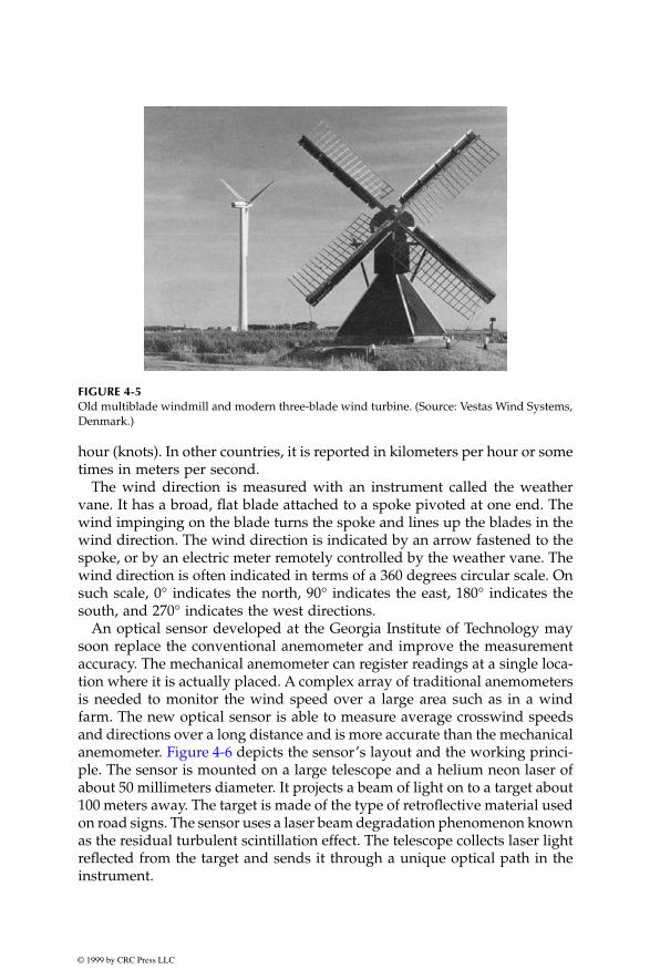
Two features of the wind, its speed, and the direction, are used in describ-ing and forecasting weather (Figure 4-5). The speed is measured with aninstrument called anemometer, which comes in several types. The mostcommon type has three or four cups attached to
spokes on a rotating shaft.The wind turns the cups and the shaft. The angular speed of the spinningshaft is calibrated in terms of the linear speed of the wind. In the UnitedStates, the wind speed is reported in miles per hour or in nautical miles per
ρ ρ= ⋅−
o
H
em0 297
3048.
ρ ρ= − ⋅ ⋅−o mH1 194 10 4.
THm= − °15 5
19 833048
..
C
© 1999 by CRC Press LLC
hour (knots). In other countries, it is reported in kilometers per hour or sometimes in meters per second.
The wind direction is measured with an instrument called the weathervane. It has a broad, flat blade attached to a spoke pivoted at one end. Thewind impinging on the blade turns the spoke and lines up the blades in thewind direction. The wind direction is indicated by an arrow fastened to thespoke, or by an electric meter remotely controlled by the weather vane. Thewind direction is often indicated in terms of a 360 degrees circular scale. Onsuch scale, 0° indicates the north, 90° indicates the east, 180° indicates thesouth, and 270° indicates the west directions.
An optical sensor developed at the Georgia Institute of Technology maysoon replace the conventional anemometer and improve the measurementaccuracy. The mechanical anemometer can register readings at a single loca-tion where it is actually placed. A complex array of traditional anemometersis needed to monitor the wind speed over a large area such as in a windfarm. The new optical sensor is able to measure average crosswind speedsand directions over a long distance and is more accurate than the mechanicalanemometer. Figure 4-6 depicts the sensor’s layout and the working princi-ple. The sensor is mounted on a large telescope and a helium neon laser ofabout 50 millimeters diameter. It projects a beam of light on to a target about100 meters away. The target is made of the type of retroflective material usedon road signs. The sensor uses a laser beam degradation phenomenon knownas the residual turbulent scintillation effect. The telescope collects laser lightreflected from the target and sends it through a unique optical path in theinstrument.
FIGURE 4-5
Old multiblade windmill and modern three-blade wind turbine. (Source: Vestas Wind Systems,Denmark.)

© 1999 by CRC Press LLC
Each of the two tiny detectors monitors a spot on the target inside the laserbeam and picks up shadowy waves or fringes moving across the laser beam.The waves are
visible on the target itself. The fringes look much like theshadows of waves seen at the bottom of a swimming pool on a sunny day.Something akin to these shadows can be seen if a turbulent wind is viewedwith a laser beam. Each detector registers the moment when a dark fringepasses its view. By digitizing the detected points, a computer can measuretime and separation, and, therefore, the average wind speed.
The major advantage
of the optical sensor is that it can measure the windspeed over a wide range from a faint wind to a wild wind over a large area.
4.6 Wind Speed Distribution
Having the cubic relation with the power, the wind speed is the most criticaldata needed to appraise the power potential of a candidate site. The windis never steady at any site. It is influenced by the weather system, the localland terrain, and the height above the ground surface. The wind speed variesby the minute, hour, day, season, and year. Therefore, the annual mean speedneeds to be averaged over 10 or more years. Such a long term average raisesthe confidence in assessing the energy-capture potential of a site. However,long-term measurements are expensive, and most projects cannot wait thatlong. In such situations, the short term, say one year, data is compared witha nearby site having a long term data to predict the long term annual windspeed at the site under consideration. This is known as the “measure, cor-relate and predict (mcp)” technique.
FIGURE 4-6
Optical wind speed sensor construction. (Source: Georgia Institute of Technology, Atlanta, GA.With permission.)

© 1999 by CRC Press LLC
Since wind is driven by the sun and the seasons, the wind pattern generallyrepeats over the period of one year. The wind site is usually described bythe speed data averaged over the calendar months. Sometimes, the monthlydata is aggregated over the year for brevity in reporting the overall “wind-iness” of various sites. The wind-speed variations over the period can bedescribed by a probability distribution function.
4.6.1 Weibull Probability Distribution
The variation in wind speed are best described by the Weibull probabilitydistribution function ‘h’ with two parameters, the shape parameter ‘k’, andthe scale parameter ‘c’. The probability of wind speed being v during anytime interval is given by the following:
(4-19)
In the probability distribution chart, h is plotted against v over a chosentime period, where:
(4-20)
By definition of the probability function, probability that the wind speedwill be between zero and infinity during that period is unity, i.e.:
(4-21)
If we choose the time period of one year, then express the probabilityfunction in terms of the number of hours in the year, such that:
(4-22)
The unit of ‘h’ is hours per year per meter/second, and the integral (4-21)becomes 8,760 (the total number of hours in the year) instead of unity.
Figure 4-7 is the plot of h versus v for three different values of k. The curveon the left with k = 1 has a heavy bias to the left, where most days arewindless (v=0). The curve on the right with k = 3 looks more like a normalbell shape distribution, where some days have high wind and equal number
h vkc
vc
ek v
c
k
( ) =
∞
−( ) −
1
for 0 < v <
hv
v= +( )fraction of time wind speed is between v and v ∆
∆
h dv⋅ =∞
∫ 10
hv v
v= +( )number of hours the wind is between v and ∆
∆

© 1999 by CRC Press LLC
of days have low wind. The curve in the middle with k = 2 is a typical winddistribution found at most sites. In this distribution, more days have lowerthan the mean speed, while few days have high wind. The value of kdetermines the shape of the curve, hence is called the ‘shape parameter’.
The Weibull distribution with k = 1 is called the exponential distributionwhich is generally used in the reliability studies. For k>3, it approaches thenormal distribution, often called the Gaussian or the bell-shape distribution.
Figure 4-8 shows the distribution curves corresponding to k = 2 with dif-ferent values of c ranging from 8 to 16 mph (1 mph = 0.446 m/s). For greatervalues of c, the curves shift right to the higher wind speeds. That is, the higherthe c, the more number of days have high winds. Since this shifts the distri-bution of hours at a higher speed scale, the c is called the scale parameter.
At most sites the wind speed has the Weibull distribution with k = 2, whichis specifically known as the Rayleigh distribution. The actual measurementdata taken at most sites compare well with the Rayleigh distribution, as seenin Figure 4-9. The Rayleigh distribution is then a simple and accurate enoughrepresentation of the wind speed with just one parameter, the scale param-eter “c”.
Summarizing the characteristics of the Weibull probability distributionfunction:
FIGURE 4-7
Weibull probability distribution function with scale parameter c=10 and shape parameters k =1, 2 and 3.
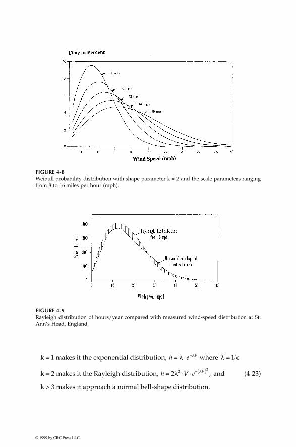
© 1999 by CRC Press LLC
(4-23)
FIGURE 4-8
Weibull probability distribution with shape parameter k = 2 and the scale parameters rangingfrom 8 to 16 miles per hour (mph).
FIGURE 4-9
Rayleigh distribution of hours/year compared with measured wind-speed distribution at St.Ann’s Head, England.
k = 1 makes it the exponential distribution, where = 1 c
k = 2 makes it the Rayleigh distribution, , and
k > 3 makes it approach a normal bell-shape distribution.
h e
h V e
V
V
= ⋅
= ⋅ ⋅
−
−( )
λ λ
λ
λ
λ2 2 2

© 1999 by CRC Press LLC
Since most wind sites would have the scale parameter ranging from 10 to20 miles per hour (about 5 to 10 m/s), and the shape parameter rangingfrom 1.5 to 2.5 (rarely 3.0), our discussion in the following sections will centeraround those ranges of c and k.
Figure 4-10 displays the number of hours on the vertical axis versus thewind speed on the horizontal axis with distributions of different scale param-eters c = 10, 15, and 20 mph and shape parameters k = 1.5, 2, and 3. Thevalues of h in all three sets of curves are the number of hours in a year inthe speed interval v +
∆
v divided by
∆
v. Figure 4-11 depicts the same plotsin the three-dimensional h-v-k space. It shows the effect of k in shifting theshape from the bell shape in the front right hand side (k = 3) to the Rayleighand flatter shapes as the value of k decreases from 3.0 to 1.5. It is alsoobserved from these plots that as c increases, the distribution shifts to thehigher speed values.
FIGURE 4-10
Weibull distributions of hours/year with three different shape parameters k = 1.5, 2, and 3.

© 1999 by CRC Press LLC
4.6.2 Mode and Mean Speeds
We now define the following terms applicable to the wind speed:Mode speed is defined as the speed corresponding to the hump in the
distribution function. This is the speed the wind blows most of the time.Mean speed
over the period is defined as the total area under the h-v curveintegrated from v = 0 to
∞
, divided by the total number of hours in the period(8,760 if the period is one year). The annual mean speed is therefore theweighted average speed and is as follows:
FIGURE 4-11
Three-dimensional h-v-k plots with c ranging from 10 to 20 mph and k ranging from 1.5 to 3.0.

© 1999 by CRC Press LLC
(4-24)
For c and k values in the range found at most sites, the integral expressioncan be approximated to the Gamma function:
(4-25)
For the Rayleigh distribution with k = 2, the Gamma function can befurther approximated to the following:
(4-26)
This is a very simple relation between the scale parameter c and V
mean
,which can be used with reasonable accuracy. For example, most sites arereported in terms of their mean wind speeds. The c parameter in the corre-sponding Rayleigh distribution is then c = V
mean
/0.9. The k parameter is ofcourse 2.0 for the Rayleigh parameters. Thus, we have the Rayleigh distri-bution of the site using the generally reported mean speed as follows:
(4-27)
4.6.3 Root Mean Cube Speed
The wind power is proportional to the speed cube, and the energy collectedover the year is the integral of h ·
v
3
·
dv. We, therefore, define the “rootmean cube” or the “rmc” speed in the manner similar to the root meansquare (rms) value in the alternating current circuits:
(4-28)
The rmc speed is useful in quickly estimating the annual energy potentialof the site. Using V
rmc
in Equation 4-12 gives the annual average power:
(4-29)
V h v dvmean = ⋅ ⋅∞
∫18760
0
)V ckmean = +
1
1
V cmean = ⋅0 90.
h vv
ce
v
Ve
vc
mean
vVmean( ) = =
( )−
−
2 2
2 2
2 2
V h v dvrmc = ⋅ ⋅∞
∫18760
3
0
3
P Vrmc rmc= ⋅14
3ρ watts m2

© 1999 by CRC Press LLC
Then, multiplying the P
rmc
value by the total number of the hours in theyear gives the annual energy production potential of the site.
The importance of the rmc speed
is highlighted in Table 4-1
.
It comparesthe wind power density at three sites with the same annual average windspeed of 6.3 m/s. The San Gorgonio site in California has 66 percent greaterpower density than the Culebra site in Puerto Rico. The difference comesfrom having the different shape factors k, and, hence, the different rmcspeeds, although all have the same annual mean speed.
4.6.4 Mode, Mean, and rmc Speeds Compared
The important difference between the mode, mean, and the rmc speeds isillustrated in Table 4-2. The values of the three speeds are compiled for fourshape parameters (k = l.5, 2.0, 2.5, and 3.0) and three scale parameters (c =10, 15, and 20 mph). The wind power densities are calculated using therespective speeds in the wind power equation
P
= 1/2
ρ
·
V
3
watts/m
2
usingthe air mass density of 1.225 kg/m
3
.We observe the following from the c=15 rows:
1. For k = 1.5, the power density using the mode speed is 230 versusthe correct value of 4,134 watts/m
2
using the rmc speed. The ratioof the incorrect to correct value of the power density is 1 to 18 —a huge difference.
2. For k = 2, the power densities using the mode and rmc speeds are731 and 2,748 watts/m
2
, respectively, in the ratio of 1 to 3.76. Thecorresponding power densities with the mean and the rmc speedsare 1,439 and 2,748 watts/m
2
in the ratio of 1 to 1.91.3. For k = 3, the power densities using the mode and rmc speeds are
1,377 and 2,067 watts/m
2
, respectively, in the ratio of 1 to 1.50. The corresponding power densities with the mean and the rmc speeds are 1,472 and 2,067 watts/m
2
, in the ratio of 1 to 1.40.
Thus, regardless of the shape and the scale parameters, use of the modeor the mean speed in the power density equation would introduce a signif-icant error in the annual energy estimate, sometimes of several folds, makingthe estimates completely useless.
TABLE 4-1
Comparison of Three Wind Farm Sites with the Same Mean Wind Speed
but Significantly Different Specific Power Density
SiteAnnual mean wind speed Annual average specific power
Meters/second Watts/m
2
Culebra, Puerto Rico 6.3 220Tiana beach, New York 6.3 285San Gorgonio, California 6.3 365

© 1999 by CRC Press LLC
The last column in Table 4-2 is the yearly energy potentials of the corre-sponding sites in kWh per year per square meter of the blade area for thegiven k and c values. These values are calculated for the rotor efficiency
C
p
of 50 percent, which is the maximum that can be practically achieved.
4.6.5 Energy Distribution
If we define the energy distribution function:
(4-30)
Then, it would look like that in Figure 4-12, which is for the Rayleigh speeddistribution. The wind speed curve has the mode at 5.5 m/s and the meanat 6.35 m/s. However, because of the cubic relation with the speed, themaximum energy contribution comes from the wind speed at 9.45 m/s.Above this speed, although V
3
continues to increase in cubic manner, thenumber of hours at those speeds decreases faster than V
3
. The result is anoverall decrease in the yearly energy contribution. For this reason, it isadvantageous to design the wind power to operate at variable speeds inorder to capture the maximum energy available during high wind periods.
Figure 4-13 is a similar chart showing the speed and energy distributionfunctions for shape parameter 1.5 and scale parameter 15 mph. The modespeed is 10.6 mph, the mean speed is 13.3 and the rmc speed is 16.5 mph.
TABLE 4-2
Influence of the Shape and Scale Parameters on the Mode, Mean and RMC
Speeds and the Energy Density
c kModeSpeed
MeanSpeed
RMCSpeed
PmodeW/m
2
PmeanW/m
2
PrmcW/m
2
ErmcKWh/yr
10 1.5 4.81 9.03 12.60 68 451 1225 53662.0 7.07 8.86 11.00 216 426 814 35652.5 8.15 8.87 10.33 331 428 675 29573.0 8.74 8.93 10.00 409 436 613 2685
15 1.5 7.21 13.54 18.90 230 1521 4134 181072.0 10.61 13.29 16.49 731 1439 2748 120362.5 12.23 13.31 15.49 1120 1444 2278 99783.0 13.10 13.39 15.00 1377 1472 2067 9053
20 1.5 9.61 18.05 25.19 544 3604 9790 428802.0 14.14 17.72 22.00 1731 3410 6514 285312.5 16.30 17.75 20.66 2652 3423 5399 236483.0 17.47 17.86 20.00 3266 3489 4900 21462
P = wind power density in watts per square meter of the blade swept area = 0.5 ρ V3
where ρ = 1.225 kg/m3
The last column is the energy potential of the site in kWh per year per m2 of theblade area, assuming the rotor efficiency Cp of 50 percent (i.e., the maximumpower that can be converted into electrical power is 0.25 ρ V3).
ev v
v= +( )kWh contribution in the year by the wind between v and ∆
∆

© 1999 by CRC Press LLC
The energy distribution function has the mode at 28.5 mph. That is, the mostenergy is captured at 28.5 mph wind speed, although the probability of windblowing at that speed is low.
The comparison of Figures 4-12 and 4-13 shows that as the shape param-eter value decreases from 2.0 to 1.5, the speed and the energy modes movefarther apart. On the other hand, as the speed distribution approaches thebell shape for k > 3, the speed and the energy modes get closer to each other.
FIGURE 4-12Rayleigh distributions of hours and energy per year versus wind speed with c = 10 and k = 2.
FIGURE 4-13Rayleigh distributions of hours and energy per year versus wind speed with c = 15 and k = 1. 5.
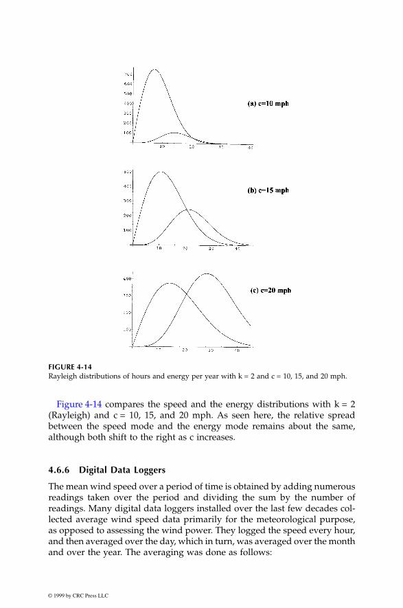
© 1999 by CRC Press LLC
Figure 4-14 compares the speed and the energy distributions with k = 2(Rayleigh) and c = 10, 15, and 20 mph. As seen here, the relative spreadbetween the speed mode and the energy mode remains about the same,although both shift to the right as c increases.
4.6.6 Digital Data Loggers
The mean wind speed over a period of time is obtained by adding numerousreadings taken over the period and dividing the sum by the number ofreadings. Many digital data loggers installed over the last few decades col-lected average wind speed data primarily for the meteorological purpose,as opposed to assessing the wind power. They logged the speed every hour,and then averaged over the day, which in turn, was averaged over the monthand over the year. The averaging was done as follows:
FIGURE 4-14Rayleigh distributions of hours and energy per year with k = 2 and c = 10, 15, and 20 mph.

© 1999 by CRC Press LLC
(4-31)
As seen earlier, for assessing the wind power, the rmc speed is whatmatters. The rmc equivalent of the digital data logging is as follows:
(4-32)
The above equation does not take into account the variation in the air massdensity, which is also a parameter (although of second order) in the windpower density. Therefore, a better method of collecting the wind power datais to digitize the yearly average power density as follows:
(4-33)
where n = number of observations in the averaging periodρi = air density (kg/m3), andVi = wind speed (m/s) at the ith observation time.
4.6.7 Effect of Height
The wind shear at ground surface causes the the wind speed increase withheight in accordance with the expression
(4-34)
where V1 = wind speed measured at the reference height h1
V2 = wind speed estimated at height h2, andα = ground surface friction coefficient.
The friction coefficient is low for smooth terrain and high for rough ones(Figure 4-15). The values of α for typical terrain classes are given in Table 4-3.
The wind speed does not increase with height indefinitely. The data col-lected at Merida airport in Mexico show that typically the wind speedincreases with height up to about 450 meter height, and then decreases(Figure 4-16)1. The wind speed at 450 meters height can be four to five timesgreater than that near the ground surface.
Vn
Vavg ii
n
==
∑1
1
Vn
Vrmc ii
n
==
∑1 3
1
3
Pn
Vrmc i ii
n
= ⋅=
∑12
3
1
ρ
2 12
1
= ⋅
Vhh
α
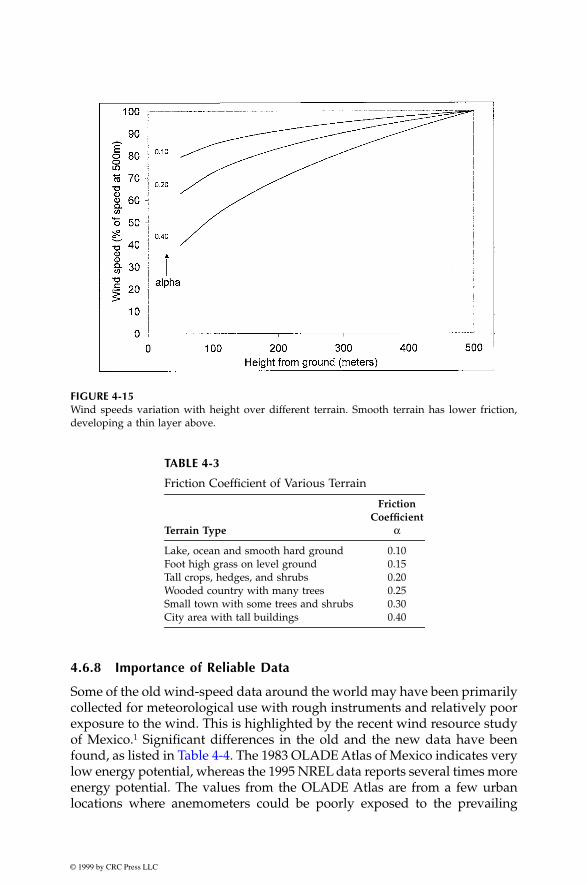
© 1999 by CRC Press LLC
4.6.8 Importance of Reliable Data
Some of the old wind-speed data around the world may have been primarilycollected for meteorological use with rough instruments and relatively poorexposure to the wind. This is highlighted by the recent wind resource studyof Mexico.1 Significant differences in the old and the new data have beenfound, as listed in Table 4-4. The 1983 OLADE Atlas of Mexico indicates verylow energy potential, whereas the 1995 NREL data reports several times moreenergy potential. The values from the OLADE Atlas are from a few urbanlocations where anemometers could be poorly exposed to the prevailing
FIGURE 4-15Wind speeds variation with height over different terrain. Smooth terrain has lower friction,developing a thin layer above.
TABLE 4-3
Friction Coefficient of Various Terrain
Terrain Type
FrictionCoefficient
α
Lake, ocean and smooth hard ground 0.10Foot high grass on level ground 0.15Tall crops, hedges, and shrubs 0.20Wooded country with many trees 0.25Small town with some trees and shrubs 0.30City area with tall buildings 0.40

© 1999 by CRC Press LLC
winds. In contrast, the new NREL wind data comes from a large number ofstations, including open airport locations, and has incorporated the terraineffect in the final numbers. The message here is clear. It is important to have
FIGURE 4-16Wind-speed variations with height measured at Merida airport in Mexico. (Source: Schwartzand Elliott, DOE/NREL Report DE95009202, May 1995.)
TABLE 4-4
Comparison of Calculated Average Wind Power Density Between 1983 OLADE Atlas and 1995 NREL Analysis for Several Locations in Mexico
Region in Mexico
Wind Power Density in Watts/meter2
Data Site
OLADEAtlas(1983)
NRELData
(1995)
Yucatan Peninsula Merida 22 165Campeche 23 120Chetumal 28 205
Northern Gulf Plain Tampico 8 205Ciudad Victoria 32 170Matamoros 32 165
Central Highlands Durango 8 140San Luis Potosi 35 155Zacatecas 94 270
Northwest Chihuahua 27 120Hermosillo 3 80La Paz 10 85
Data at 10 meters height.

© 1999 by CRC Press LLC
reliable data on the annual wind speed distribution over at least a few yearsbefore siting a wind farm with a high degree of confidence.
4.7 Wind Speed Prediction
The available wind energy depends on the wind speed, which is a randomvariable. For the wind-farm operator, this poses difficulty in the systemscheduling and energy dispatching, as the schedule of the wind-power avail-ability is not known in advance. However, if the wind speed can be reliablyforecasted up to several hours in advance, the generating schedule canefficiently accommodate the wind generation. Alexiadis et al2 have proposeda new technique for forecasting wind speed and power output up to severalhours in advance. The technique is based on cross-correlation at neighboringsites and artificial neutral networks. The proposed technique can signifi-cantly improve forecasting accuracy compared to the persistence forecastingmodel. The new proposed method is calibrated at different sites over a one-year period.
4.8 Wind Resource Maps
The wind resource of a vast region or a country is mapped in terms of thewind speed, the wind power density in watts per square meter of the rotorswept area, or the wind energy potential in kWh/m2 per year. Often the windresource is mapped in all three forms. The data is usually represented by thecontour curves, as it is the most useful and easily understood mapping tech-nique. Along the contour line, the plotted parameter remains constant. Forexample, the isovent map plots the contour lines connecting the sites havingthe same annual wind speed. The equipotential map plots the contour linesconnecting the sites having the same annual wind energy capture potential inkWh/m2. The wind resource maps of many countries have been prepared insuch contour form. Some of them are presented in the following sections:
4.8.1 The U.S.A.
The U.S. wind resource is large enough to produce more than 4.4 trillion kWhof electricity each year. This is more than the entire nation will use in theyear 2000. Figure 4-17 is the wind speed map of the U.S.A., whereasFigure 4-18 is the wind power density map.3-4 Although most of the country’sinstalled wind capacity is presently in California, the Department of Energyestimates that almost 90 percent of the usable wind resource in the U.S.A.

© 1999 by CRC Press LLC
FIGURE 4-17Annual average wind-power density in watts/m2 in the U.S.A. at a 50-meter tower height.(Source: DOE/NREL.)
FIGURE 4-18The U.S. wind resource map. (Source: DOE/Battelle Pacific Northwest Laboratory.)
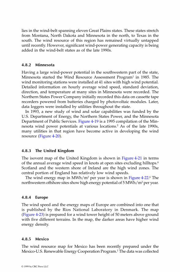
© 1999 by CRC Press LLC
lies in the wind-belt spanning eleven Great Plains states. These states stretchfrom Montana, North Dakota and Minnesota in the north, to Texas in thesouth. The wind resource of this region has remained virtually untappeduntil recently. However, significant wind-power generating capacity is beingadded in the wind-belt states as of the late 1990s.
4.8.2 Minnesota
Having a large wind-power potential in the southwestern part of the state,Minnesota started the Wind Resource Assessment Program1 in 1985. Thewind monitoring stations were installed at 41 sites with high wind potential.Detailed information on hourly average wind speed, standard deviation,direction, and temperature at many sites in Minnesota were recorded. TheNorthern States Power Company initially recorded this data on cassette taperecorders powered from batteries charged by photovoltaic modules. Later,data loggers were installed by utilities throughout the state.
In 1993, a new study of wind and solar capabilities was funded by theU.S. Department of Energy, the Northern States Power, and the MinnesotaDepartment of Public Services. Figure 4-19 is a 1995 compilation of the Min-nesota wind power potentials at various locations.5 As of the late 1990s,many utilities in that region have become active in developing the windresource (Figure 4-20).
4.8.3 The United Kingdom
The isovent map of the United Kingdom is shown in Figure 4-21 in termsof the annual average wind speed in knots at open sites excluding hilltops.6Scotland and the western shore of Ireland are the high wind zones. Thecentral portion of England has relatively low wind speeds.
The wind energy map in MWh/m2 per year is shown in Figure 4-22.6 Thenorthwestern offshore sites show high energy potential of 5 MWh/m2 per year.
4.8.4 Europe
The wind speed and the energy maps of Europe are combined into one thatis published by the Rios National Laboratory in Denmark. The map(Figure 4-23) is prepared for a wind tower height of 50 meters above groundwith five different terrains. In the map, the darker areas have higher windenergy density.
4.8.5 Mexico
The wind resource map for Mexico has been recently prepared under theMexico-U.S. Renewable Energy Cooperation Program.1 The data was collected

© 1999 by CRC Press LLC
at numerous city and airport sites spread throughout the country as shownin Figure 4-24. The maps, based on the extensive data collected at thoselocations, are separately reported for the utility-scale power generation andfor the stand-alone remote power generation. This distinction is usefulbecause the wind speed needed to make the wind farm economical for ruralapplication is less than that required for the utility scale application.
Figure 4-25 is the utility-scale wind resource map for Mexico. The highestwind potential for grid-connected power plants is in the Zacatecas and thesouthern Isthmus of Tehuantepec areas. The rural wind resource map in
FIGURE 4-19Minnesota wind resource map. (Source: Minnesota wind resources assessment program,Department of Public Service Report, 1994.)

© 1999 by CRC Press LLC
Figure 4-26 shows that areas suitable for stand-alone remote wind farms arewidespread, and include about one-half of Mexico.
4.8.6 India
The wind speed measurement stations in India have been in operation sinceearly 1980 at numerous locations. Sites with high wind speeds are shown inFigure 4-27, and their annual mean speed listed in Table 4-5. The data hasbeen collected at 10-m or 25-m tower heights as indicated.7 It is seen thatmost of these sites have the annual mean wind speed exceeding 18 km/h,which generally makes the wind power plant economically viable. The stateswith high wind potentials are Tamilnadu, Gujarat (Figure 4-28) and AndhraPradesh.
FIGURE 4-20U.S. utilities gaining experience in developing wind power generation projects. (Source: Windenergy program overview, DOE Report No. 10095-071, March 1995.)
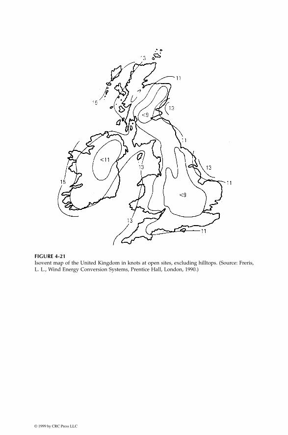
© 1999 by CRC Press LLC
FIGURE 4-21Isovent map of the United Kingdom in knots at open sites, excluding hilltops. (Source: Freris,L. L., Wind Energy Conversion Systems, Prentice Hall, London, 1990.)
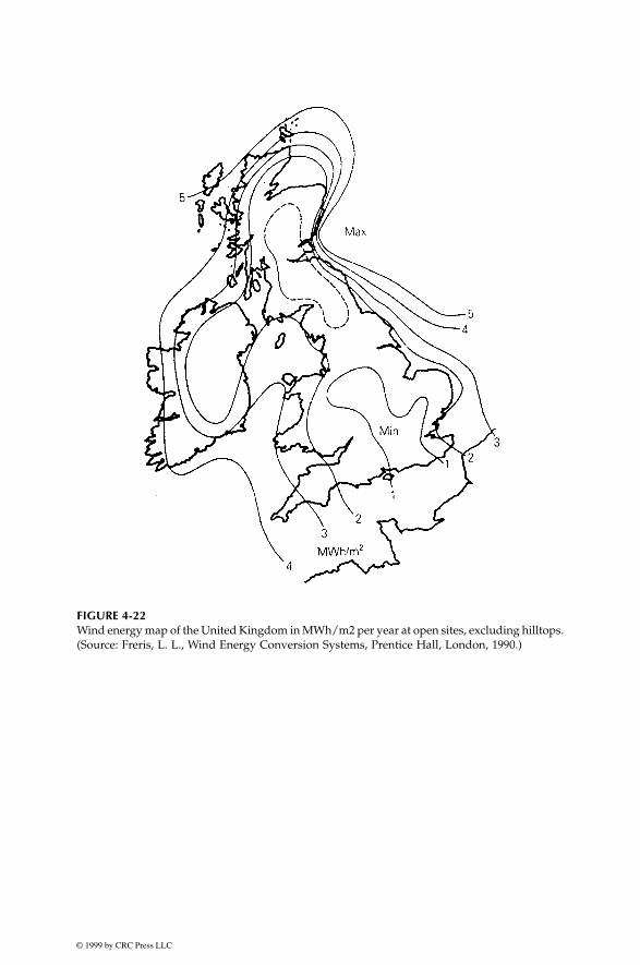
© 1999 by CRC Press LLC
FIGURE 4-22Wind energy map of the United Kingdom in MWh/m2 per year at open sites, excluding hilltops.(Source: Freris, L. L., Wind Energy Conversion Systems, Prentice Hall, London, 1990.)

© 1999 by CRC Press LLC
FIGURE 4-23European wind resource map. (Source: Risø Laboratory, Denmark.)

© 1999 by CRC Press LLC
FIGURE 4-24Locations in Mexico with surface wind data in DATSAV2 data set. (Source: Schwartz, M. N.and Elliott, D. L., Mexico wind resource assessment project, DOE/NREL Report No.DE95009202, March 1995.)

© 1999 by CRC Press LLC
FIGURE 4-25Annual average wind resource map of Mexico for utility scale applications. (Source: Schwartz,M. N. and Elliott, D. L., Mexico wind resource assessment project, DOE/NREL Report No.DE95009202, March 1995.)
FIGURE 4-26Annual average wind resource map of Mexico for rural power applications. (Source: Schwartz,M. N. and Elliott, D. L., Mexico wind resource assessment project, DOE/NREL Report No.DE95009202, March 1995.)
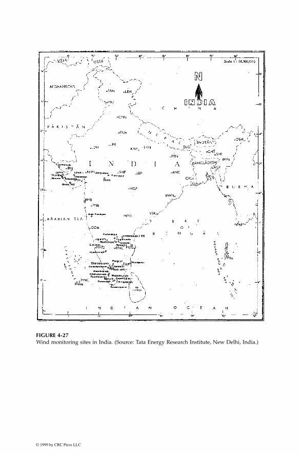
© 1999 by CRC Press LLC
FIGURE 4-27Wind monitoring sites in India. (Source: Tata Energy Research Institute, New Delhi, India.)

© 1999 by CRC Press LLC
TABLE 4-5
Mean Annual Wind Speed at Selected Sites in India
Site km/h Site km/h
Sites with 25–30 km/h wind speed Sites with 15–20 km/h wind speed
Ramakalmedu 30.3 Onamkulam* 19.9Jogmatti 30.0 Nettur* 19.9B.& H. Hills 27.1 Gude Panchgani 119.8Dhank-2 25.1 Bhandariya 19.5
Sites with 20–25 km/h wind speed Ramagiri-3 19.4Poosaripatti* 19.3Pongalur 19.1
Dhank-1 24.4 Limbara 19.1Singanamala 23.8 Jamalamadugu-2* 18.7Edayarpalayam 22.4 Ottapidaram 18.5Kadavakallu* 22.1 Ponmudi 18.3Kalyanpur 22.1 Hardenahalli 18.2Kumarapuram* 22.0 Kheda 18.2Kethanur 21.1 Jamgodrani 18.0Navadra 20.8 Jamalamadunga-1* 17.5Arasampalayam 20.5 Poompuhar 17.2Bamambore-2 20.3 Minicoy 17.0Mustikovala 20.2 Kolahalamendu 16.9Pancjalimedu 20.2 Naduvakkurichi 16.8Lamda 20.0 Yeradoddi* 15.8
Mirzapur 15.4
* Data at 25-m height, all others at 10-m height
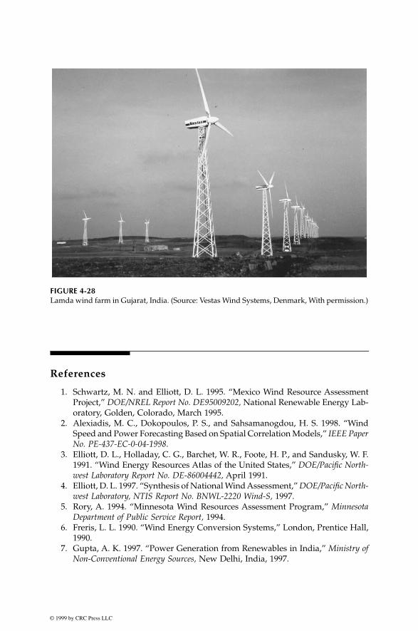
© 1999 by CRC Press LLC
References
1. Schwartz, M. N. and Elliott, D. L. 1995. “Mexico Wind Resource AssessmentProject,” DOE/NREL Report No. DE95009202, National Renewable Energy Lab-oratory, Golden, Colorado, March 1995.
2. Alexiadis, M. C., Dokopoulos, P. S., and Sahsamanogdou, H. S. 1998. “WindSpeed and Power Forecasting Based on Spatial Correlation Models,” IEEE PaperNo. PE-437-EC-0-04-1998.
3. Elliott, D. L., Holladay, C. G., Barchet, W. R., Foote, H. P., and Sandusky, W. F.1991. “Wind Energy Resources Atlas of the United States,” DOE/Pacific North-west Laboratory Report No. DE-86004442, April 1991.
4. Elliott, D. L. 1997. “Synthesis of National Wind Assessment,” DOE/Pacific North-west Laboratory, NTIS Report No. BNWL-2220 Wind-S, 1997.
5. Rory, A. 1994. “Minnesota Wind Resources Assessment Program,” MinnesotaDepartment of Public Service Report, 1994.
6. Freris, L. L. 1990. “Wind Energy Conversion Systems,” London, Prentice Hall,1990.
7. Gupta, A. K. 1997. “Power Generation from Renewables in India,” Ministry ofNon-Conventional Energy Sources, New Delhi, India, 1997.
FIGURE 4-28Lamda wind farm in Gujarat, India. (Source: Vestas Wind Systems, Denmark, With permission.)

© 1999 by CRC Press LLC
5
Wind Power System
The wind power system is fully covered in this and the following twochapters. This chapter covers the overall system level performance, designconsiderations and trades. The electrical generator is covered in the nextchapter and the speed control in Chapter 7.
5.1 System Components
The wind power system is comprised of one or more units, operating elec-trically in parallel, having the following components:
• the tower.• the wind turbine with two or three blades.• the yaw mechanism such as the tail vane.• the mechanical gear.• the electrical generator.• the speed sensors and control.
The modern system often has the following additional components:
• the power electronics.• the control electronics, usually incorporating a computer.• the battery for improving the load availability in stand-alone mode.• the transmission link connecting to the area grid.
Because of the large moment of inertia of the rotor, the design challengesinclude the starting, the speed control during the power producing opera-tion, and stopping the turbine when required. The eddy current or othertype of brake is used to halt the turbine when needed for emergency or forroutine maintenance. In the multiple tower wind farm, each turbine must
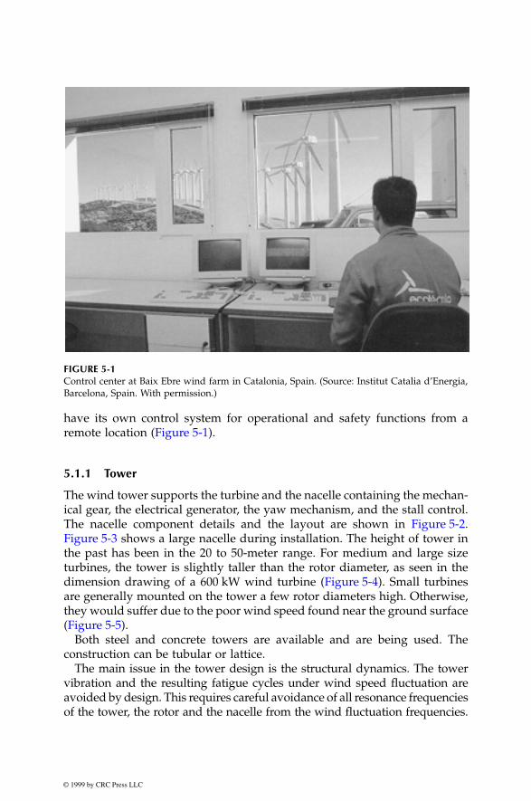
© 1999 by CRC Press LLC
have its own control system for operational and safety functions from aremote location (Figure 5-1).
5.1.1 Tower
The wind tower supports the turbine and the nacelle containing the mechan-ical gear, the electrical generator, the yaw mechanism, and the stall control.The nacelle component details and the layout are shown in Figure 5-2.Figure 5-3 shows a large nacelle during installation. The height of tower inthe past has been in the 20 to 50-meter range. For medium and large sizeturbines, the tower is slightly taller than the rotor diameter, as seen in thedimension drawing of a 600 kW wind turbine (Figure 5-4). Small turbinesare generally mounted on the tower a few rotor diameters high. Otherwise,they would suffer due to the poor wind speed found near the ground surface(Figure 5-5).
Both steel and concrete towers are available and are being used. Theconstruction can be tubular or lattice.
The main issue in the tower design is the structural dynamics. The towervibration and the resulting fatigue cycles under wind speed fluctuation areavoided by design. This requires careful avoidance of all resonance frequenciesof the tower, the rotor and the nacelle from the wind fluctuation frequencies.
FIGURE 5-1
Control center at Baix Ebre wind farm in Catalonia, Spain. (Source: Institut Catalia d’Energia,Barcelona, Spain. With permission.)

© 1999 by CRC Press LLC
Sufficient margin must be maintained between the two sets of frequenciesin all vibrating modes.
The resonance frequencies of the structure are determined by completemodal analyses, leading to the eigenvectors and eigenvalues of complexmatrix equations representing the motion of the structural elements. Thewind fluctuation frequencies that are found form the measurements at thesite under consideration. Experience on a similar nearby site can bridge agap on the required information.
Big cranes are generally required to install wind towers. Gradually increas-ing tower height, however, is bringing a new dimension in the installation(Figure 5-6). Large rotors add to the transportation problem as well. Tillabletowers to nacelle and rotors moving upwards along with the tower areamong some of the newer developments in the wind tower installation. Theoffshore installation comes with its own challenge that must be met.
5.1.2 Turbine Blades
The turbine blades are made of high-density wood or glass fiber and epoxycomposites. Modern wind turbines have two or three blades. The steady
FIGURE 5-2
Nacelle details of a 150 kW/25 meter diameter turbine. (Source: Nordtank Energy Group/NEGMicon, Denmark. With permission.)

© 1999 by CRC Press LLC
mechanical stress due to centrifugal forces and fatigue under continuous vibra-tions make the blade design the weakest mechanical link in the system. Exten-sive design effort is needed to avoid premature fatigue failure of the blade.
The mechanical stress in the blade under gusty wind is kept under theallowable limit. This is achieved by controlling the rotor speed below the setlimit. This not only protects the blades, but also protects the electrical gen-erator from overloading and overheating. One method that has been usedfrom the early designs and continues to be used today is the stall control.At stall, the wind flow ceases to be smooth around the blade contour, butseparates before reaching the trailing edge. This always happens at highpitch angle. The blades experience high drag, thus lowering the rotor poweroutput. The high pitch angle also produces high lift. The resulting load onthe blade can cause a high level of vibration and fatigue, possibly leadingto the mechanical failure. Regardless of the fixed or variable speed, the designengineer must deal with the stall forces. Researchers are moving from
FIGURE 5-3
A large nacelle under installation. (Source: Nordtank Energy Group/NEG Micon, Denmark. Withpermission.)

© 1999 by CRC Press LLC
the 2D to 3D stress analyses to better understand and design for such forces.As a result, the blade design is continually changing, particularly at the bladeroot where the loading is maximum due to the cantilever effect.
The aerodynamic design of the blade is important, as it determines theenergy capture potential. The large and small machine blades have signifi-cantly different design philosophies. The small machine sitting on the tower
FIGURE 5-4
A 600 kW wind turbine and tower dimensions with specifications. (Source: Wind World Cor-poration, Denmark. With permission.)

© 1999 by CRC Press LLC
relatively taller than the blade diameter, and generally unattended, requireslow maintenance design. On the other hand, the large machine tends tooptimize the aerodynamic performance for the maximum possible energycapture. In either case, the blade cost is generally kept below 10 percent ofthe total installed cost.
5.1.3 Yaw Control
The yaw control continuously orients the rotor in the direction of the wind.It can be as simple as the tail vane, or more complex on modern towers.Theoretical considerations dictate free yaw as much as possible. However,rotating blades with large moments of inertia produce high gyroscopictorque during yaw, often resulting in loud noise. Too rapid yaw may generatenoise exceeding the local ordinance limit. Hence, a controlled yaw is oftenrequired and is used.
5.1.4 Speed Control
The wind turbine technology has changed significantly in the last 25 years.
1
Large wind turbines being installed today tend to be of variable speed
FIGURE 5-5
Tower heights of various capacity wind turbines.

© 1999 by CRC Press LLC
design, incorporating the pitch control and the power electronics. Smallmachines on the other hand must have simple, low cost power and speedcontrol. The speed control methods fall into the following categories:
• no speed control whatsoever. In this method, the turbine, the elec-trical generator, and the entire system is designed to withstand theextreme speed under gusty wind.
• yaw and tilt control, in which the rotor axis is shifted out of thewind direction when the wind speed exceeds the design limit.
• pitch control, which changes the pitch of the blade with the chang-ing wind speed to regulate the rotor speed.
• stall control. In this method of speed control, when the wind speed exceeds the safe limit on the system, the blades are shifted into a position such that they stall. The turbine has to be restarted after the gust has gone.
Figure 5-7 depicts the distribution of the control methods used in smallwind turbine designs. Large machines generally use the power electronicspeed control, which is covered in Chapters 7 and 11.
FIGURE 5-6
WEG MS-2 wind turbine installation at Myers Hill. (Source: Wind Energy Group, a TaylorWoodrow subsidiary and ETSU/DTI, U.K.)

© 1999 by CRC Press LLC
5.2 Turbine Rating
The wind turbines are manufactured in sizes ranging from a few kW forstand-alone remote applications to a couple of MW each for utility scalepower generation. The grid-connected turbine as large as 2 MW capacitywas installed in 1979 on Howard Knob Mountain in the United States, and3 MW capacity was installed in 1988 at Berger Hill in the United Kingdom.
The method of assessing the nominal rating of the wind turbine has noglobally acceptable standard. The difficulty arises because the power outputof the turbine depends on the square of the rotor diameter and the cube ofthe wind speed. The rotor of a given diameter will, therefore, generatedifferent power at different wind speed. The turbine that can generate300 kW at 7 m/s would produce 450 kW at 8 m/s wind. What rating shouldthen be assigned to this turbine? Should we also specify the “rated speed”?Early wind turbine designers created a rating system that specified the poweroutput at some arbitrary wind speed. This method did not work well aseveryone could not agree on one speed to specify the power rating. The “rated”wind speeds varied from 10 to 15 m/s under this practice. Manufacturers are
FIGURE 5-7
Speed control methods used in small to medium size turbines.

© 1999 by CRC Press LLC
lax on providing the higher side of the wind speed, claiming greater outputfrom the same design.
To avoid such rating confusion, some European manufacturers refer toonly the rotor diameter. But the confusion continues as to the maximumpower the machine can generate under the highest wind speed the turbinecan continuously operate. Many manufacturers have, therefore, adopted thecombined rating designations — the wind turbine diameter following thegenerator peak electrical rating. For example, the 300/30 wind system means300 kW electrical generator and 30-meter diameter turbine.
The specific rated capacity (SRC) is often used as a comparative index ofthe wind turbine designs. It is defined as follows:
(5-1)
For the 300/30 wind turbine, the specific rated capacity is 300/
π
15
2
=0.42 kW/m
2
. The specific rated capacity increases with the diameter, givinga favorable economy of scale to large machine. It ranges from approximately0.2 kW/m
2
for 10-meter diameter rotor to 0.5 kW/m
2
for 40-meter diameterrotor. Some aggressively rated turbines have SRC of 0.7 kW/m
2
, and somereaching as high as 1.0 kW/m
2
. The operating stresses in rotor blades of thehigh SRC are high, generally resulting in shorter fatigue life. All stressconcentration regions are carefully identified and eliminated in high SCRdesigns. Modern design tools, such as the finite element stress analysis andthe modal vibration analysis can be of great help in the rotor design.
The turbine rating is important as it indicates to the system designer howto size the induction generator, the plant’s transformer, connecting cables tothe substation, and the transmission link interfacing the grid. The powersystem must be sized on the peak capacity of the generator, and the generatoris rated in a different manner than the wind turbine. The turbine powerdepends on the cube of the wind speed. The system design engineer is,therefore, required to match the turbine and the generator performancecharacteristics. This means selecting the rated speed of the turbine to matchwith the generator. Since the gearbox and the generator are manufacturedonly in discrete sizes, selecting the turbine rated speed can be complex. Theselection process goes through several iterations, trading the cost with benefitof the available speeds. Selecting a low rated speed would result in wastingmuch energy at high winds. On the other hand, if the rated speed is high,the rotor efficiency will suffer most of the times.
Figure 5-8 is an example of the summary data sheet of the 550/41 kW/mwind turbine manufactured by Nordtank Energy Group of Denmark. Suchdata is used in the preliminary design of the overall system. The specificrated capacity of this machine is 0.415. It has the cut-in wind speed of 5 m/s,the cutout speed of 25 m/s and it reaches the peak power at 15 m/s.
SRC = Generator electrical capacityRotor swept area

© 1999 by CRC Press LLC
FIGU
RE 5-8
Technical data sheet of a 550 kW
/41-m
eter diam
eter wind
turbine, with pow
er level and noise level. (Source: N
ordtank
Energy G
roup, Denm
ark. With perm
ission.)
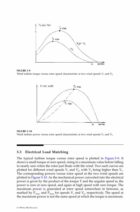
© 1999 by CRC Press LLC
5.3 Electrical Load Matching
The typical turbine torque versus rotor speed is plotted in Figure 5-9. Itshows a small torque at zero speed, rising to a maximum value before fallingto nearly zero when the rotor just floats with the wind. Two such curves areplotted for different wind speeds V
1
and V
2
, with V
2
being higher than V
1
.The corresponding powers versus rotor speed at the two wind speeds areplotted in Figure 5-10. As the mechanical power converted into the electricalpower is given by the product of the torque
Τ
and the angular speed
ω,
thepower is zero at zero speed, and again at high speed with zero torque. Themaximum power is generated at rotor speed somewhere in between, asmarked by P
1max
and P
2max
for speeds V
1
and V
2
, respectively. The speed atthe maximum power is not the same speed at which the torque is maximum.
FIGURE 5-9
Wind turbine torque versus rotor speed characteristic at two wind speeds V
1
and V
2
.
FIGURE 5-10
Wind turbine power versus rotor speed characteristic at two wind speeds V
1
and V
2
.

© 1999 by CRC Press LLC
The operating strategy of a well-designed wind power system is to matchthe load on the electrical generator so that the rotor operates continuouslyat speeds as close as possible to the P
max
points. Since the P
max
point changeswith the wind speed, the rotor speed must therefore be adjusted in accor-dance with the wind speed to make the rotor work continuously at P
max
.
5.4 Variable-Speed Operation
At a given site, the wind speed can vary from zero to high gust. As discussedin Chapter 4, the Rayleigh statistical distribution is found to be the bestapproximation to represent the wind speed at most sites. It varies over awide range. Earlier in Chapter 4, we defined the tip-speed ratio as follows:
(5-2)
where R and
ω
are the rotor radius and the angular speed, respectively.For a given wind speed, the rotor efficiency C
p
varies with TSR as shownin Figure 5-11. The maximum value of C
p
occurs approximately at the samewind speed that gives peak power in the power distribution curve ofFigure 5-10. To capture the high power at high wind, the rotor must alsoturn at high speed, keeping the TSR constant at the optimum level.
Three system performance attributes are related to the TSR:
• The centrifugal mechanical stress in the blade material is propor-tional to the TSR. The machine working at a higher TSR is stressedmore. Therefore, if designed for the same power in the same windspeed, the machine operating at a higher TSR would have slimmerrotor blades.
• The ability of a wind turbine to start under load is inversely pro-portional to the design TSR. As this ratio increases, the startingtorque produced by the blade decreases.
• As seen above, the TSR is also related to the operating point for extracting the maximum power. The maximum rotor efficiency C
p
is achieved at a particular TSR, which is specific to the aerodynamic design of a given turbine. The TSR needed for the maximum power extraction ranges from nearly one for multiple-blade, slow-speed machines to nearly six for modern high-speed, two-blade machines.
The wind power system design must optimize the annual energy captureat a given site. The only operating mode for extracting the maximum energyis to vary the turbine speed with varying wind speed such that at all timesthe TSR is continuously equal to that required for the maximum power
TSRR
V= = ⋅Linear speed of the blade outer most tip
Free upstream wind velocityω

© 1999 by CRC Press LLC
coefficient Cp. The theory and field experience indicates that the variable-speed operation yields 20 to 30 percent more energy than with the fixed-speed operation. Nevertheless, cost of the variable-speed control is added.In the system design, this trade-off between the energy increase and the costincrease has to be optimized. In the past, the added costs of designing thevariable-pitch rotor, or the speed control with power electronics, outweighedthe benefit of the increased energy capture. However, falling prices of thepower electronics for speed control, and availability of high-strength fibercomposites for constructing high-speed rotors, have made it economical tocapture more energy when the speed is high. In the fixed-speed operation,on the other hand, the rotor is shut off during high-wind speeds, losingsignificant energy. The pros and cons of the variable and the fixed-speedoperations are listed in Table 5-1.
5.5 System Design Features
The following additional design trade-offs are available to the system engineer:
5.5.1 Number of Blades
This is the first determination the design engineer must make. Windmachines have been built with the number of blades ranging from 2 to 40
FIGURE 5-11
Rotor efficiency and annual energy production versus rotor tip-speed ratio.

© 1999 by CRC Press LLC
or more. The high number of blades was used in old low, tip-speed ratiorotors for water pumping, the application which needs high starting torque.The modern high, tip-speeds ratio rotors for generating electrical power havetwo or three blades, many of them with just two. The major factors involvedin deciding the number of blades are as follows:
• the effect on power coefficient.• the design tip-speeds ratio.• the cost.• the nacelle weight.• the structural dynamics.• the means of limiting yaw rate to reduce gyroscopic fatigue.
Compared to the two-blade design, the three-blade machine has smootherpower output and balanced gyroscopic force. There is no need to teeter therotor, allowing the use of simple rigid hub. Three blades are more commonin Europe, where large machines up to 1 MW are being developed using thethree-blade configuration. The American practice, however, has been in thetwo blade designs. Adding the third blade increases the power coefficientonly by about 5 percent, thus giving a diminished rate of return for the50 percent more weight and cost. The two-blade rotor is also simpler to erect,since it can be assembled on the ground and lifted to the shaft withoutcomplicated maneuvers during the lift. The number of blades is often viewedas the blade solidity. Higher solidity ratio gives higher starting torque andoperates at low speed. For electrical power generation, the turbine must runat high speed since the electrical generator weighs less and operates moreefficiently at high speed. That is why all large-scale wind turbines have lowsolidity ratio, with just two or three blades.
TABLE 5-1
Advantages of Fixed and Variable Speed Systems
Fixed-Speed System Variable-Speed System
Simple and inexpensive electrical system Higher rotor efficiency, hence, higher energy capture per year
Fewer parts, hence higher reliability Low transient torqueLower probability of excitation of mechanical resonance of the structure
Fewer gear steps, hence inexpensive gear box
No frequency conversion, hence, no current harmonics present in the electrical system
Mechanical damping system not needed, the electrical system could provide damping if required
Lower capital cost No synchronization problems Stiff electrical controls can reduce system voltage sags

© 1999 by CRC Press LLC
5.5.2 Rotor Upwind or Downwind
Operating the rotor upwind of the tower produces higher power as it elim-inates the tower shadow on the blades. This also results in lower noise, lowerblade fatigue, and smoother power output. The downwind blades, on theother hand, allow the use of free yaw system. It also allows the blades todeflect away from the tower when loaded. Both types are used at presentwith no clear trend.
5.5.3 Horizontal Axis Versus Vertical Axis
Most wind turbines built at present have a horizontal axis. The vertical axisDarrieus machine has several advantages. First of all, it is omnidirectionaland requires no yaw mechanism to continuously orient itself toward thewind direction. Secondly, its vertical drive shaft simplifies the installation ofthe gearbox and the electrical generator on the ground, making the structuremuch simpler. On the negative side, it normally requires guy wires attachedto the top for support. This could limit its applications, particularly for theoffshore sites. Overall, the vertical axis machine has not been widely usedbecause its output power cannot be easily controlled in high winds simplyby changing the blade pitch. With modern low-cost, variable-speed powerelectronics emerging in the wind power industry, the Darrieus configurationmay revive, particularly for large capacity applications.
5.5.4 Spacing of the Towers
When installing a cluster of machines in a wind farm, certain spacingbetween the wind towers must be maintained to optimize the power crop-ping. The spacing depends on the terrain, the wind direction, the speed, andthe turbine size. The optimum spacing is found in rows 8 to 12-rotor diam-eters apart in the wind direction, and 1.5 to 3-rotor diameters apart in thecrosswind direction (Figure 5-12). A wind farm consisting of 20 towers ratedat 500 kW each need 1 to 2 square kilometers of land area. Of this, only acouple of percent would actually occupy the tower and the access roads.The remaining land could continue its original use (Figure 5-13). The averagenumber of machines in wind farms varies greatly, ranging from several tohundreds depending on the required power capacity.
When the land area is limited or is at a premium price, one optimizationstudy that must be conducted in an early stage of the wind farm design isto determine the number of turbines, their size, and the spacing for extract-ing the maximum energy from the farm. The trades in such a study are asfollows:
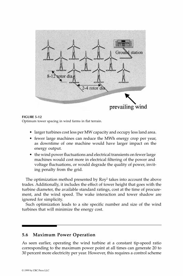
© 1999 by CRC Press LLC
• larger turbines cost less per MW capacity and occupy less land area.• fewer large machines can reduce the MWh energy crop per year,
as downtime of one machine would have larger impact on theenergy output.
• the wind power fluctuations and electrical transients on fewer large machines would cost more in electrical filtering of the power and voltage fluctuations, or would degrade the quality of power, invit-ing penalty from the grid.
The optimization method presented by Roy
2
takes into account the abovetrades. Additionally, it includes the effect of tower height that goes with theturbine diameter, the available standard ratings, cost at the time of procure-ment, and the wind speed. The wake interaction and tower shadow areignored for simplicity.
Such optimization leads to a site specific number and size of the windturbines that will minimize the energy cost.
5.6 Maximum Power Operation
As seen earlier, operating the wind turbine at a constant tip-speed ratiocorresponding to the maximum power point at all times can generate 20 to30 percent more electricity per year. However, this requires a control scheme
FIGURE 5-12
Optimum tower spacing in wind farms in flat terrain.

© 1999 by CRC Press LLC
to operate with variable speed. Two possible schemes used with the variable-speed operation are as follows:
5.6.1 Constant Tip-Speed Ratio Scheme
This scheme is based on the fact that the maximum energy is extracted whenthe optimum tip-speed ratio is maintained constantly at all wind speeds.The optimum TSR is a characteristic of the given wind turbine. This optimumvalue is stored as the reference TSR in the control computer. The wind speedis continuously measured and compared with the blade tip speed. The errorsignal is then fed to the control system, which changes the turbine speed tominimize the error (Figure 5-14). At this time the rotor must be operating atthe reference TSR generating the maximum power. This scheme has a dis-advantage of requiring the local wind speed measurements, which could
FIGURE 5-13
Original land use continues in a wind farm in Germany. (Source: Vestas Wind Systems, DenmarkWith permission.)

© 1999 by CRC Press LLC
have significant error particularly in a large wind farm with shadow effects.Being sensitive to the changes in the blade surface, the optimum TSR grad-ually changes. The computer reference TSR must be changed accordinglymany times over the life. This is expensive. Besides, it is difficult to determinethe new optimum tip-speed ratio with changes that are not fully understood,nor easily measured.
5.6.2 Peak Power Tracking Scheme
The power versus speed curve has a single well-defined peak. If we operateat the peak point, a small increase or decrease in the turbine speed wouldresult in no change in the power output, as the peak point locally lies in aflat neighborhood. Therefore, a necessary condition for the speed to be atthe maximum power point is as follows:
(5-3)
This principle is used in the control scheme (Figure 5-15). The speed isincreased or decreased in small increments, the power is continuously mea-sured, and
∆
P
/
∆ω
is continuously evaluated. If this ratio is positive, meaningwe get more power by increasing the speed, the speed is further increased.On the other hand, if the ratio is negative, the power generation will reduceif we change the speed any further. The speed is maintained at the levelwhere
∆
P
/
∆ω
is close to zero. This method is insensitive to the errors in localwind speed measurement, and also to the wind turbine design. It is, there-fore, the preferred method. In a multiple machine wind farm, each turbinemust be controlled by its own control loop with operational and safetyfunctions incorporated.
FIGURE 5-14
Maximum power operation using rotor tip-speed control scheme.
dPdω
= 0

© 1999 by CRC Press LLC
5.7 System Control Requirements
5.7.1 Speed Control
The rotor speed must be controlled for three reasons:
• to capture more energy, as seen above.• to protect the rotor, the generator and the power electronic equip-
ment from overloading at high wind.• when the generator is disconnected accidentally or for a scheduled
event, losing the electrical load. Under this condition, the rotor speed may run away, destroying it mechanically, if it is not controlled.
The speed control requirement of the rotor has five separate regions(Figure 5-16):
1. The cut-in speed at which the turbine starts producing power.Below this speed, it is not efficient to turn on the turbine.
2. The constant maximum C
p
region where the rotor speed varieswith the wind-speed variation to operate at the constant TSR cor-responding to the maximum C
p
value.3. During high winds, the rotor speed is limited to an upper constant
limit based on the design limit of the system components. In theconstant speed region, the C
p
is lower than the maximum C
p
, andthe power increases at a lower rate than that in the first region.
4. At still higher wind speeds, such as during a gust, the machine isoperated at constant power to protect the generator and the power
FIGURE 5-15
Maximum power operation using power control scheme.
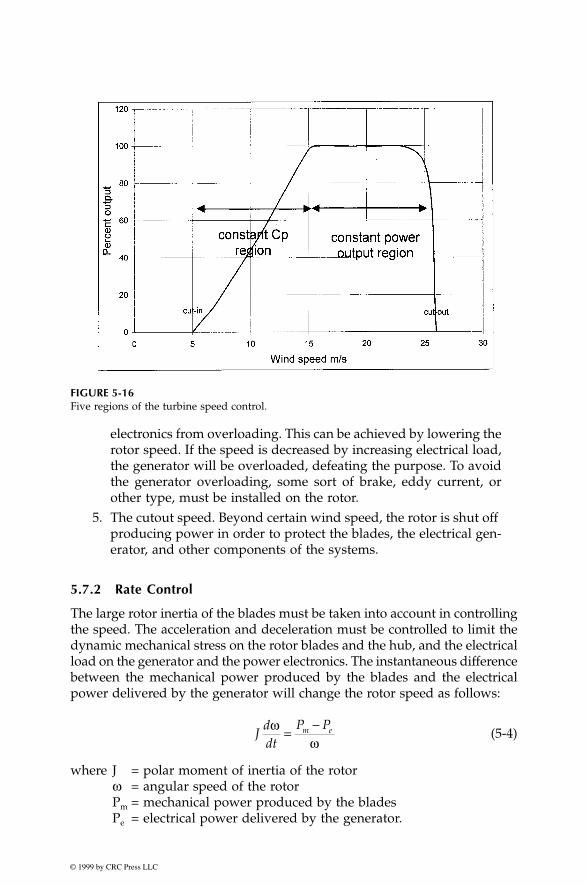
© 1999 by CRC Press LLC
electronics from overloading. This can be achieved by lowering therotor speed. If the speed is decreased by increasing electrical load,the generator will be overloaded, defeating the purpose. To avoidthe generator overloading, some sort of brake, eddy current, orother type, must be installed on the rotor.
5. The cutout speed. Beyond certain wind speed, the rotor is shut off producing power in order to protect the blades, the electrical gen-erator, and other components of the systems.
5.7.2 Rate Control
The large rotor inertia of the blades must be taken into account in controllingthe speed. The acceleration and deceleration must be controlled to limit thedynamic mechanical stress on the rotor blades and the hub, and the electricalload on the generator and the power electronics. The instantaneous differencebetween the mechanical power produced by the blades and the electricalpower delivered by the generator will change the rotor speed as follows:
(5-4)
where J = polar moment of inertia of the rotor
ω
= angular speed of the rotorP
m
= mechanical power produced by the bladesP
e
= electrical power delivered by the generator.
FIGURE 5-16
Five regions of the turbine speed control.
Jddt
P Pm eωω
=−
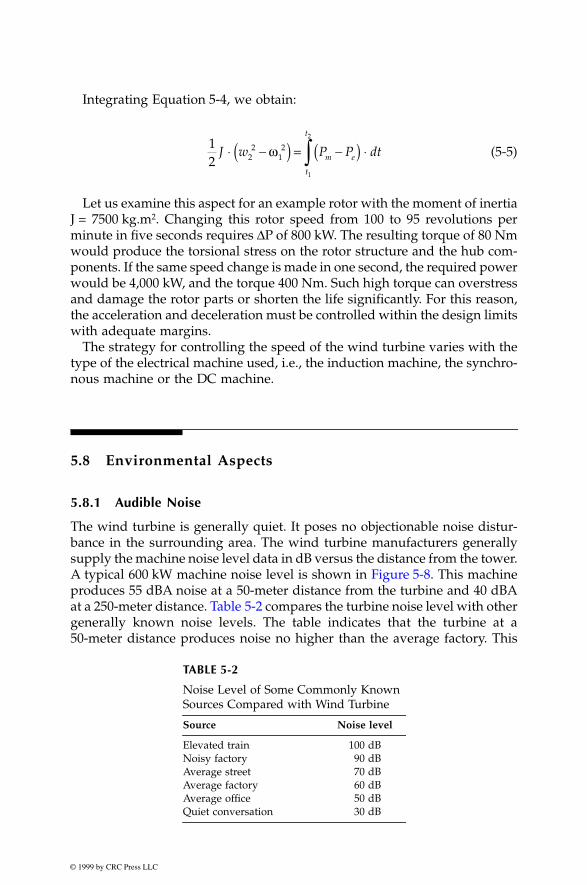
© 1999 by CRC Press LLC
Integrating Equation 5-4, we obtain:
(5-5)
Let us examine this aspect for an example rotor with the moment of inertiaJ = 7500 kg.m
2
. Changing this rotor speed from 100 to 95 revolutions perminute in five seconds requires
∆
P of 800 kW. The resulting torque of 80 Nmwould produce the torsional stress on the rotor structure and the hub com-ponents. If the same speed change is made in one second, the required powerwould be 4,000 kW, and the torque 400 Nm. Such high torque can overstressand damage the rotor parts or shorten the life significantly. For this reason,the acceleration and deceleration must be controlled within the design limitswith adequate margins.
The strategy for controlling the speed of the wind turbine varies with thetype of the electrical machine used, i.e., the induction machine, the synchro-nous machine or the DC machine.
5.8 Environmental Aspects
5.8.1 Audible Noise
The wind turbine is generally quiet. It poses no objectionable noise distur-bance in the surrounding area. The wind turbine manufacturers generallysupply the machine noise level data in dB versus the distance from the tower.A typical 600 kW machine noise level is shown in Figure 5-8. This machineproduces 55 dBA noise at a 50-meter distance from the turbine and 40 dBAat a 250-meter distance. Table 5-2 compares the turbine noise level with othergenerally known noise levels. The table indicates that the turbine at a50-meter distance produces noise no higher than the average factory. This
TABLE 5-2
Noise Level of Some Commonly Known
Sources Compared with Wind Turbine
Source Noise level
Elevated train 100 dBNoisy factory 90 dBAverage street 70 dBAverage factory 60 dBAverage office 50 dBQuiet conversation 30 dB
12 2
212
1
2
J w P P dtm e
t
t
⋅ −( ) = −( ) ⋅∫ω

© 1999 by CRC Press LLC
noise, however, is a steady noise. The turbine makes loud noise while yawingunder the changing wind direction. The local noise ordinance must be com-plied with. There have been cases of noise complaints reported by the nearbycommunities.
5.8.2 Electromagnetic Interference (EMI)
Any stationary or moving structure in the proximity of a radio or TV towerinterferes with the signals. The wind turbine towers, being large structures,can cause objectionable electromagnetic interference on the performance ofthe nearby transmitters or receivers. Additionally, rotor blades of an operat-ing wind turbine may reflect impinging signals so that the electromagneticsignals in the neighborhood may experience interference at the blade passagefrequency. The exact nature and magnitude of such EMI depend on a numberof parameters. The primary parameters are the location of the wind turbinetower relative to the radio or TV tower, physical and electrical properties ofthe rotor blades, the signal frequency modulation scheme, and the high-frequency electromagnetic wave propagation characteristics in the localatmosphere.
3
In other aspects, the visual impact of the wind farm along with the effecton the wind life can be of concern to some. The breeding and feeding patternsof the birds may be disturbed. They may even be injured and killed if theycollide with the blades. Under these concerns, obtaining permission fromthe local planning authorities can take considerable time and effort.
References
1. Roy, S. 1997. “Optimal planning of wind energy conversion systems over anenergy scenario,”
IEEE Transaction on Energy Conversion,
September 1997.2. Gijs, van Kuik. 1998. “Wind turbine technology — 25 years’ progress”
WindDirections,
April 1998.3. Spera, D. A. 1994. “Wind Turbine Technology,”
American Society of MechanicalEngineers,
New York, 1994.

© 1999 by CRC Press LLC
6
Electrical Generator
6.1 Electromechanical Energy Conversion
The conversion of the mechanical power of the wind turbine into the elec-trical power can be accomplished by any one of the following types of theelectrical machines
:
• the direct current (DC) machine.• the synchronous machine.• the induction machine.
These machines work on the principles of the electromagnetic actions andreactions. The resulting electromechanical energy conversion is reversible.The same machine can be used as the motor for converting the electricalpower into mechanical power, or as the generator converting the mechanicalpower into the electrical power.
Figure 6-1 depicts common features of the electrical machines. Typically,there is an outer stationary member (stator) and an inner rotating member(rotor). The rotor is mounted on bearings fixed to the stator. Both the statorand the rotor carry cylindrical iron cores, which are separated by an air gap.The cores are made of magnetic iron of high permeability, and have conduc-tors embedded in slots distributed on the core surface. Alternatively, theconductors are wrapped in the coil form around salient magnetic poles.Figure 6-2 is the cross-sectional view of the rotating electrical machine withthe stator with salient poles and the rotor with distributed conductors. Themagnetic flux, created by the excitation current in one of the two members,passes from one core to the other in the combined magnetic circuit alwaysforming a closed loop. The electromechanical energy conversion is accom-plished by interaction of the magnetic flux produced by one member withthe electric current in the other member. The latter may be externally sup-plied or electromagnetically induced. The induced current is proportionalto the rate of change in the flux linkage due to rotation.
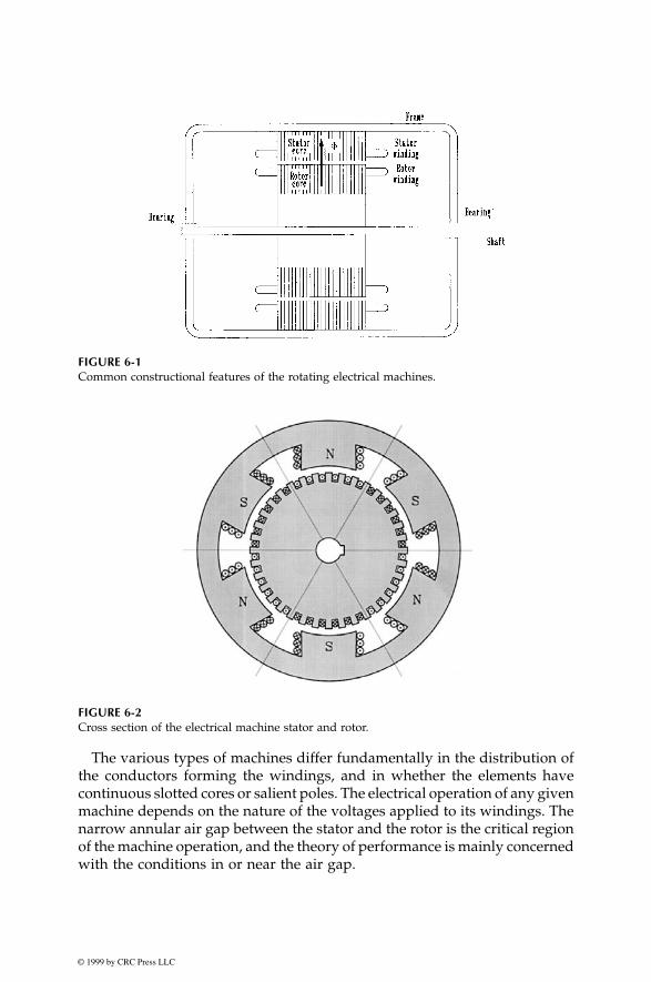
© 1999 by CRC Press LLC
The various types of machines differ fundamentally in the distribution ofthe conductors forming the windings, and in whether the elements havecontinuous slotted cores or salient poles. The electrical operation of any givenmachine depends on
the nature of the voltages applied to its windings. Thenarrow annular air gap between the stator and the rotor is the critical regionof the machine operation, and the theory of performance is mainly concernedwith the conditions in or near the air gap.
FIGURE 6-1
Common constructional features of the rotating electrical machines.
FIGURE 6-2
Cross section of the electrical machine stator and rotor.

© 1999 by CRC Press LLC
6.1.1 DC Machine
All machines are internally alternating current (AC) machines because of theconductor rotation in the magnetic flux of alternate north and south polarity.The DC machine must convert the AC into DC, and does so by using themechanical commutator. The commutator performs this function by slidingcarbon brushes on a series of copper segments. The positive output terminalis, thus, continuously switched to the conductor generating the positivepolarity voltage, as is the negative polarity terminal. The sliding contactsinherently result in low reliability and high maintenance cost. Despite thisdisadvantage, the DC machine had been used extensively until early 1980sbecause of its extremely easy speed control. It has been used in a limitednumber of wind power installations of small capacity, particularly whereelectricity can be locally used in the DC form. However, the conventionalDC machine with mechanical commutator has fallen out of favor.
The conventional DC machine is either self-excited by shunt or series coilscarrying DC current to produce a magnetic field. The DC machine of thepresent day is often designed with permanent magnets to eliminate the fieldcurrent requirement, hence, the commutator. It is designed in the “inside-out” configuration. The rotor carries the permanent magnet poles and thestator carries the wound armature which produces AC current. The AC isthen rectified using the solid state rectifiers. Such machines do not need thecommutator and the brushes, hence, the reliability is greatly improved. Thepermanent magnet DC machine is used with small wind turbines, however,due to limitation of the permanent magnet capacity and strength. The brush-less DC machine is expected to be limited to ratings below one hundred kW.
6.1.2 Synchronous Machine
Most of the electrical power consumed in the world is generated by thesynchronous generator. For this reason, the synchronous machine is an estab-lished machine. The machine works at a constant speed related to the fixedfrequency. Therefore, it is not well suited for variable-speed operation in thewind plants. Moreover, the synchronous machine requires DC current toexcite the rotor field, which needs sliding carbon brushes on slip rings onthe rotor shaft. This poses a limitation on its use. The need of the DC fieldcurrent and the brushes can be eliminated by using the reluctance rotor,where the synchronous operation is achieved by the reluctance torque. Thereliability is greatly improved while reducing the cost. The machine rating,however, is limited to tens of kW. The reluctance synchronous generator isbeing investigated at present for small wind generators.
1
The synchronous machine is ideally suited in constant-speed systems, suchas in the solar thermal power plants. The machine is, therefore, covered insome detail in Chapter 9.

© 1999 by CRC Press LLC
Unlike the induction machine covered later in this chapter, the synchro-nous machine, when used in the grid-connected system, has some advan-tage. It does not require the reactive power from the grid. This results in abetter quality of power at the grid interface. This advantage is more pro-nounced when the wind farm is connected to a small capacity grid usinglong low voltage lines. For this reason, early California plants used synchro-nous generators. Today’s wind plants generally connect to larger grids usingshorter lines, and almost universally use the induction generator.
6.1.3 Induction Machine
Most of the electrical power in the industry is consumed by the inductionmachine driving the mechanical load. For this reason, the induction machinerepresents a well established technology. The primary advantage of theinduction machine is the rugged brushless construction and no need forseparate DC field power. The disadvantages of both the DC machine andthe synchronous machine are eliminated in the induction machine, resultingin low capital cost, low maintenance, and better transient performance. Forthese reasons, the induction generator is extensively used in small and largewind farms and small hydroelectric power plants. The machine is availablein numerous power ratings up to several megawatts capacity, and evenlarger.
The induction machine needs AC excitation current. The machine is eitherself-excited or externally excited. Since the excitation current is mainly reac-tive, a stand-alone system is self-excited by shunt capacitors. The inductiongenerator connected to the grid draws the excitation power from the net-work. The synchronous generators connected to the network must be capableof supplying this reactive power.
For economy and reliability, many wind power systems use inductionmachines as the electrical generator. The remaining part of this chapter is,therefore, devoted to the construction and the theory of operation of theinduction generator.
6.2 Induction Generator
6.2.1 Construction
In the electromagnetic structure of the induction generator, the stator is madeof numerous coils with three groups (phases), and is supplied withthree-phase current. The three coils are physically spread around the statorperiphery and carry currents which are out of time-phase. This combinationproduces a rotating magnetic field, which is a key feature of the working of
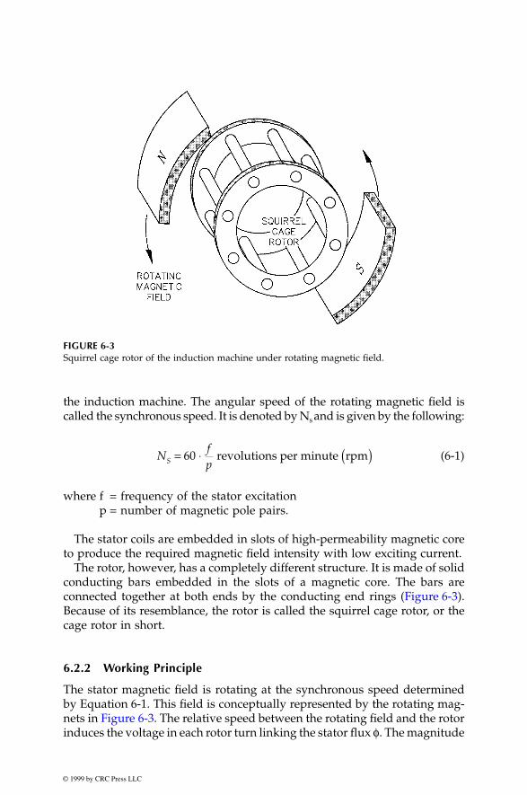
© 1999 by CRC Press LLC
the induction machine. The angular speed of the rotating magnetic field iscalled the synchronous speed. It is denoted by N
s
and is given by the following:
(6-1)
where f = frequency of the stator excitationp = number of magnetic pole pairs.
The stator coils are embedded in slots of high-permeability magnetic coreto produce the required magnetic field intensity with low exciting current.
The rotor, however, has a completely different structure. It is made of solidconducting bars embedded in the slots of a magnetic core. The bars areconnected together at both ends by the conducting end rings (Figure 6-3).Because of its resemblance, the rotor is called the squirrel cage rotor, or thecage rotor in short.
6.2.2 Working Principle
The stator magnetic field is rotating at the synchronous speed determinedby Equation 6-1. This field is conceptually represented by the rotating mag-nets in Figure 6-3. The relative speed between the rotating field and the rotorinduces the voltage in each rotor turn linking the stator flux
φ
. The magnitude
FIGURE 6-3
Squirrel cage rotor of the induction machine under rotating magnetic field.
NfpS = ⋅ ( )60 revolutions per minute rpm

© 1999 by CRC Press LLC
of the induced voltage is given by Faraday’s law of electromagnetic induc-tion, namely:
(6-2)
where
φ
= the magnetic flux linking the rotor turn.This voltage in turn sets up the circulating current in the rotor. The elec-
tromagnetic interaction of the rotor current and the stator flux produces thetorque. The amplitude of this torque is given by the following:
(6-3)
where K = constant of proportionality
Φ
= amplitude of the stator flux waveI
2
= amplitude of induced current in the rotor bars
φ
2
= phase angle by which the rotor current lags the rotor voltage.
The rotor will accelerate under this torque. If the rotor was on frictionlessbearings with no mechanical load attached, it is completely free to rotatewith zero resistance. Under this condition, the rotor will attain the samespeed as the stator field, namely, the synchronous speed. At this speed, thecurrent induced in the rotor speed is zero, no torque is produced and noneis required. The rotor finds equilibrium at this speed and will continue torun at the synchronous speed.
If the rotor is now attached to a mechanical load such as a fan, it will slowdown. The stator flux, which always rotates at the constant, synchronousspeed, will have relative speed with respect to the rotor. As a result, theelectromagnetically induced voltage, current, and torque are produced inthe rotor. The torque produced must equal that needed to drive the load atthat speed. The machine works as the motor in this condition.
If we attach the rotor to a wind turbine and drive it faster than the syn-chronous speed, the induced current and the torque in the rotor reverse thedirection. The machine now works as the generator, converting the mechan-ical power of the turbine into electrical power delivered to the load connectedto the stator terminals. If the machine was connected to a grid, it would feedpower into the grid.
Thus, the induction machine can work as the electrical generator only atspeeds higher than the synchronous speed. The generator operation, for thatreason, is often called the super-synchronous speed operation of the induc-tion machine.
As described above, the induction machine needs no electrical connectionbetween the stator and the rotor. Its operation is entirely based on theelectromagnetic induction, hence, the name. The absence of rubbing electricalcontacts and simplicity of its construction make the induction generator very
eddt
= − φ
T K I= ⋅ ⋅ ⋅Φ 2 2cosφ

© 1999 by CRC Press LLC
robust, reliable, and a low-cost machine. For this reason, it is widely usedin numerous applications in the industry.
The working principle of the induction machine can be seen as the trans-former. The high voltage coil on the stator is excited and the low voltagecoil on the rotor is shorted on itself. The power from one to the other canflow in either direction. The theory of operation of the transformer, therefore,holds true when modified to account for the relative motion between thestator and the rotor. This motion is expressed in terms of the slip of the rotorrelative to the synchronously rotating magnetic field.
6.2.3 Rotor Speed and Slip
The slip of the rotor is defined as the ratio of the speed of the rotatingmagnetic field sweeping past the rotor and the synchronous speed of thestator magnetic field. That is,
(6-4)
where s = slip of the rotorN
s
= synchronous speed = 60·f/pN
r
= rotor speed.
The slip is generally considered positive in the motoring operation. In thegenerator mode, the slip would therefore be negative. In both the motoringmode and the generating mode, higher rotor slips induce higher current inthe rotor and higher electromechanical power conversion. In both modes,the value of the slip is generally a few to several percent. Higher slips resultin greater electrical loss, which must be effectively dissipated from the rotorto keep the operating temperature below the allowable limit.
The heat is removed from the machine by the fan blades attached to oneend-ring of the rotor. The fan is enclosed in a shroud at the end. The forcedair travels axially along the machine exterior, which has fins to increase thedissipation area. Figure 6-4 is an exterior view of a 150 kW induction machineshowing the end shroud and the cooling fins running axially. Figure 6-5 is acutaway view of the machine interior of a 2 MW induction machine.
The induction generator feeding the 60 or 50 Hz grid must run at speedhigher than 3,600 rpm in a two-pole design, 1,800 rpm in a four-pole design,and 1,200 rpm in a six-pole design. The wind turbine speed, on the other hand,varies from a few hundred rpm in the kW range machines to a few tens ofrpm in the MW rage machines. The wind turbine therefore must interface thegenerator via a mechanical gear. Since this somewhat degrades the efficiencyand reliability, many small stand-alone plants operate with custom designedgenerators operating at lower speed without the mechanical gear.
sN N
Ns r
s
=−
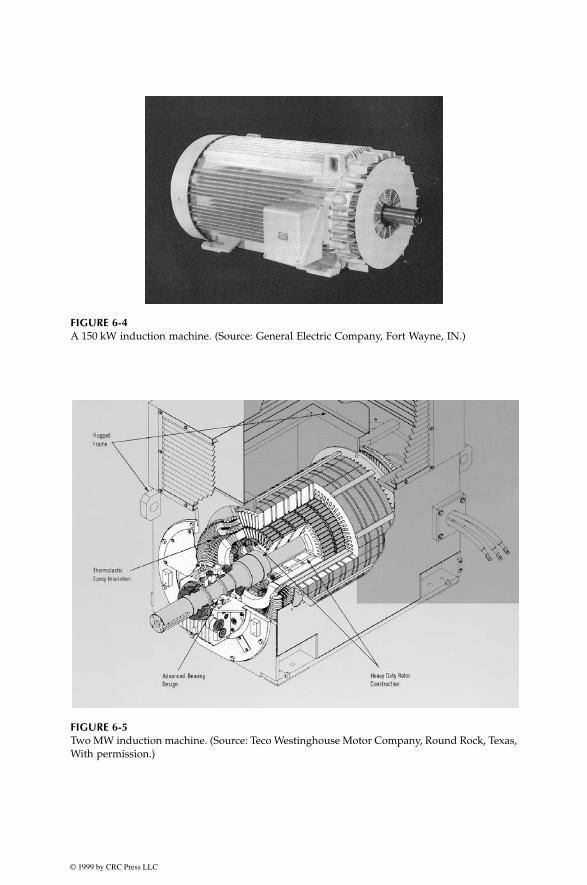
© 1999 by CRC Press LLC
FIGURE 6-4
A 150 kW induction machine. (Source: General Electric Company, Fort Wayne, IN.)
FIGURE 6-5
Two MW induction machine. (Source: Teco Westinghouse Motor Company, Round Rock, Texas,With permission.)
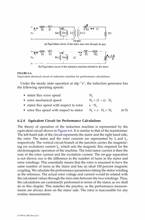
© 1999 by CRC Press LLC
Under the steady state operation at slip “s”, the induction generator hasthe following operating speeds:
• stator flux wave speed N
s
• rotor mechanical speed N
r
= (1 – s) · N
s
• stator flux speed with respect to rotor s · N
s
• rotor flux speed with respect to stator N
r
+ s · N
s
= N
s
(6-5)
6.2.4 Equivalent Circuit for Performance Calculations
The theory of operation of the induction machine is represented by theequivalent circuit shown in Figure 6-6. It is similar to that of the transformer.The left-hand side of the circuit represents the stator and the right hand side,the rotor. The stator and the rotor currents are represented by I
1
and I
2
,respectively. The vertical circuit branch at the junction carries the magnetiz-ing (or excitation) current I
o
, which sets the magnetic flux required for theelectromagnetic operation of the machine. The total stator current is then thesum of the rotor current and the excitation current. The air-gap separationis not shown, nor is the difference in the number of turns in the stator androtor windings. This essentially means that the rotor is assumed to have thesame number of turns as the stator and has an ideal 100 percent magneticcoupling. We calculate the performance parameters taking the stator windingas the reference. The actual rotor voltage and current would be related withthe calculated values through the turn ratio between the two windings. Thus,the calculations are customarily performed in terms of the stator, as we shalldo in this chapter. This matches the practice, as the performance measure-ments are always done on the stator side. The rotor is inaccessible for anyroutine measurements.
FIGURE 6-6
Equivalent electrical circuit of induction machine for performance calculations.

© 1999 by CRC Press LLC
Most of the flux links both the stator and the rotor. The flux which doesnot link both is called the leakage flux. The leakage flux is represented bythe leakage reactance. One-half of the total leakage reactance is attributed toeach side, namely the stator leakage reactance X
1
and the rotor leakagereactance X
2
in Figure 6-6(b). The stator and the rotor conductor resistanceare represented by R
1
and R
2
, respectively. The magnetizing parameters X
m
and R
m
represent the permeability and losses (hysteresis and eddy current)in the magnetic circuit of the machine.
The slip dependent rotor resistance R
2
· (1-s)/s represents the electrome-chanical power conversion. The power conversion per phase of the three-phase machine is given by I
22
R
2
· (1 –s)/s. The three-phase power conversionis then as follows:
(6-6)
The machine capacity rating is the power developed under rated condi-tions, that is as follows:
(6-7)
The electromechanical power conversion given by Equation 6-6 is physi-cally appreciated as follows. If the machine is not loaded and has zerofriction, it runs at the synchronous speed, the slip is zero and the value ofR
2
(1–s)/s becomes infinite. The rotor current is then zero, and so is P
em
, asit should be. When the rotor is standing still, the slip is unity and the valueof R
2
· (1–s)/s is zero. The rotor current is not zero, but the P
em
is zero, as themechanical power delivered by the standstill rotor is zero.
At any slip other than zero or unity, neither the rotor current nor the speedis zero, resulting in a non-zero value of P
em
.The mechanical torque is given by the power divided by the angular speed,
that is as follows:
(6-8)
where T
em
= electromechanical torque developed in the rotor in new-ton-meters
ω
= angular speed of the rotor = 2
π
.N
s
· (1–s)/60 in mechanical radi-ans/sec.
Combining the above equations, we obtain the torque at any slip s, as follows:
(6-9)
The value of 1
2
in equation (6-9) is determined by the equivalent circuitparameters, and is slip dependent. The torque developed by the induction
P I R 1 s s wattsem = ⋅ ⋅ −( )⋅3 22
2 .
Machine Rating =P
kW orP
horsepowerem rated em rated
1000 746 .
T Pem em= ω
T N I R s Newton-metersem s 22= π( )180 2 2.
© 1999 by CRC Press LLC
machine rotor is, therefore, highly slip-dependent, as is discussed later inthis chapter.
We take a note here that the performance of the induction machine iscompletely determined by the equivalent circuit parameters. The circuitparameters are supplied by the machine manufacturer, but can be deter-mined by two basic tests on the machine. The full-speed test under no loadand the zero-speed test with blocked rotor determine the complete equiva-lent circuit of the machine.
2-3
The equivalent circuit parameters are generally expressed in perunit oftheir respective rated values per phase. The rated impedance per phase isdefined as the following:
(6-10)
For example, the perunit (pu) stator resistance is expressed as the following:
(6-11)
and similar expressions for all other circuit parameters. When expressed assuch, X
1
and X
2
are equal, each a few to several percent. The R
1
and R
2
areapproximately equal, each a few percent of the rated impedance.
The mag-netizing parameters X
m
and R
m
are usually large, in several hundred percentof Z
rated
, hence, drawing negligible current compared to the rated current.For this reason, the magnetizing branch of the circuit is often ignored inmaking approximations of the machine performance calculations.
All of the above performance equations hold true for both the inductionmotor and the induction generator by taking the proper sign of the slip. Inthe generator mode, the value of the slip is negative in the performanceequations
wherever it appears. We must also remember that the real poweroutput is negative, that is the shaft receives power instead of delivering it.The reactive power drawn from the stator terminals remains lagging withrespect to the line voltage, hence, we say that the induction generator deliversleading reactive power. Both of these mean that the magnetizingvolt-amperes are supplied by an external source.
6.2.5 Efficiency and Cooling
The values of R
1
and R
2
in the equivalent circuit represent electrical lossesin the stator and the rotor, respectively. As will be seen later, for a well-designed machine, the magnetic core loss must equal the conductor
loss.Therefore, with R
1
and R
2
expressed in perunit of the base impedance, theinduction machine efficiency is approximately equal to the following:
Zrated = Rated voltage per phaseRated current per phase
ohms.
RR
perunit11= in ohms
Z in ohmsrated
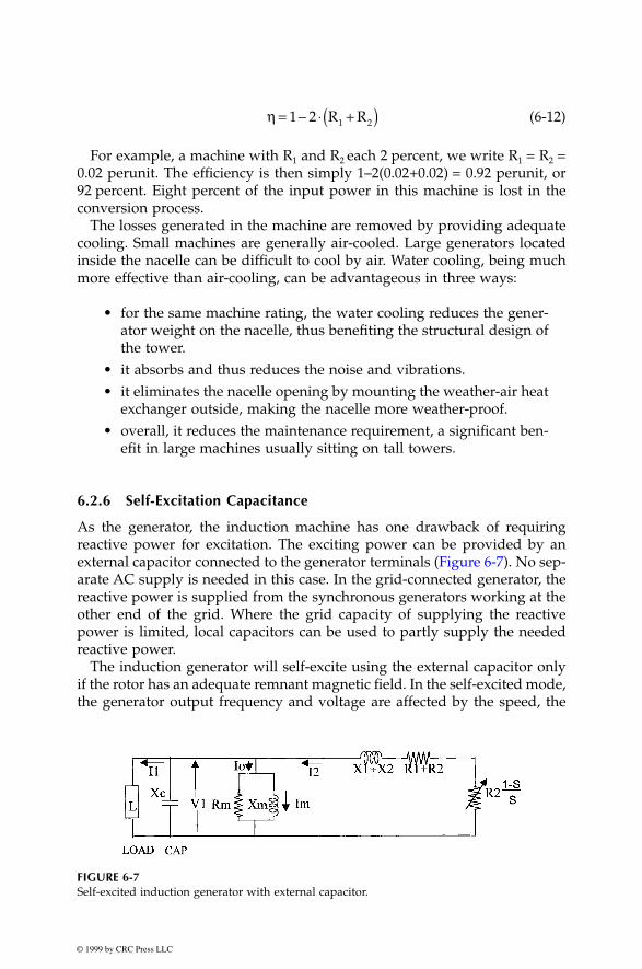
© 1999 by CRC Press LLC
(6-12)
For example, a machine with R
1
and R
2
each 2 percent, we write R
1
= R
2
=0.02 perunit. The efficiency is then simply 1–2(0.02+0.02) = 0.92 perunit, or92 percent. Eight percent of the input power in this machine is lost in theconversion process.
The losses generated in the machine are removed by providing adequatecooling. Small machines are generally air-cooled. Large generators locatedinside the nacelle can be difficult to cool by air. Water cooling, being muchmore effective than air-cooling, can be advantageous in three ways:
• for the same machine rating, the water cooling reduces the gener-ator weight on the nacelle, thus benefiting the structural design ofthe tower.
• it absorbs and thus reduces the noise and vibrations.• it eliminates the nacelle opening by mounting the weather-air heat
exchanger outside, making the nacelle more weather-proof.• overall, it reduces the maintenance requirement, a significant ben-
efit in large machines usually sitting on tall towers.
6.2.6 Self-Excitation Capacitance
As the generator, the induction machine has one drawback of requiringreactive power for excitation. The exciting power can be provided by anexternal capacitor connected to the generator terminals (Figure 6-7). No sep-arate AC supply is needed in this case. In the grid-connected generator, thereactive power is supplied from the synchronous generators working at theother end of the grid. Where the grid capacity of supplying the reactivepower is limited, local capacitors can be used to partly supply the neededreactive power.
The induction generator will self-excite using the external capacitor onlyif the rotor has an adequate remnant magnetic field. In the self-excited mode,the generator output frequency and voltage are affected by the speed, the
FIGURE 6-7
Self-excited induction generator with external capacitor.
η = − ⋅ +( )1 2 1 2R R
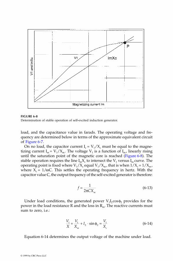
© 1999 by CRC Press LLC
load, and the capacitance value in farads. The operating voltage and fre-quency are determined below in terms of the approximate equivalent circuitof Figure 6-7.
On no load, the capacitor current I
c
= V
1
/X
c
must be equal to the magne-tizing current I
m
= V
1
/X
m
. The voltage V
1
is a function of I
m
, linearly risinguntil the saturation point of the magnetic core is reached (Figure 6-8). Thestable
operation requires the line I
m
X
c
to intersect the V
1
versus I
m
curve. Theoperating point is fixed where V
1
/X
c
equal V
1
/X
m
, that is when 1/X
c
= 1/X
m
,where X
c
= 1/
ω
C. This settles the operating frequency in hertz. With thecapacitor value C, the output frequency of the self-excited generator is therefore:
(6-13)
Under load conditions, the generated power V
1
I
2
cos
φ
2
provides for thepower in the load resistance R and the loss in R
m
. The reactive currents mustsum to zero, i.e.:
(6-14)
Equation 6-14 determines the output voltage of the machine under load.
FIGURE 6-8
Determination of stable operation of self-excited induction generator.
fCXm
=π
12
VX
VX
IVXm c
1 12 2
1+ + ⋅ =sin φ

© 1999 by CRC Press LLC
The Equations 6-13 and 6-14 determine the induction generator outputfrequency and voltage with a given value of the capacitance. Inversely, theycan be used to determine the required value of the capacitance for the desiredfrequency and the voltage.
6.2.7 Torque-Speed Characteristic
If we vary the slip over a wide range in the equivalent circuit, we get thetorque-speed characteristic as shown in Figure 6-9. In the region of negativeslip, the machine works as the generator powering the electrical load con-nected to its terminals. In the region of positive slip, it works as the motorturning the mechanical load connected to its shaft. In addition to the motor-ing and the generating regions, the induction machine has yet a third oper-ating mode, and that is the braking mode. If the machine is operated at slips>1 by turning it backward, it absorbs power without putting anything out.That is, it works as a brake. The power in this case is converted into 1
2
Rloss in the rotor conductors, which must be dissipated as heat. The eddycurrent brake works on this principle. As such, in case of emergencies, thegrid-connected induction generator can be used as brake by reversing thethree-phase voltage sequence at the stator terminals. This reverses the direction
FIGURE 6-9
Torque versus speed characteristic of the induction machine in three operating modes.
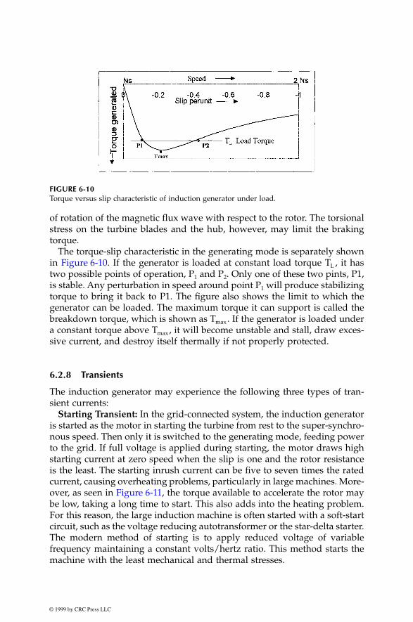
© 1999 by CRC Press LLC
of rotation of the magnetic flux wave with respect to the rotor. The torsionalstress on the turbine blades and the hub, however, may limit the brakingtorque.
The torque-slip characteristic in the generating mode is separately shownin Figure 6-10. If the generator is loaded at constant load torque T
L
, it hastwo possible points of operation, P
1
and P
2
. Only one of these two pints, P1,is stable. Any perturbation in speed around point P
1
will produce stabilizingtorque to bring it back to P1. The figure also shows the limit to which thegenerator can be loaded. The maximum torque it can support is called thebreakdown torque, which is shown as T
max
. If the generator is loaded undera constant torque above T
max
, it will become unstable and stall, draw exces-sive current, and destroy itself thermally if not properly protected.
6.2.8 Transients
The induction generator may experience the following three types of tran-sient currents:
Starting Transient:
In the grid-connected system, the induction generatoris started as the motor in starting the turbine from rest to the super-synchro-nous speed. Then only it is switched to the generating mode, feeding powerto the grid. If full voltage is applied during starting, the motor draws highstarting current at zero speed when the slip is one and the rotor resistanceis the least. The starting inrush current can be five to seven times the ratedcurrent, causing overheating problems, particularly in large machines. More-over, as seen in Figure 6-11, the torque available to accelerate the rotor maybe low, taking a long time to start. This also adds into the heating problem.For this reason, the large induction machine is often started with a soft-startcircuit, such as the voltage reducing autotransformer or the star-delta starter.The modern method of starting is to apply reduced voltage of variablefrequency maintaining a constant volts/hertz ratio. This method starts themachine with the least mechanical and thermal stresses.
FIGURE 6-10
Torque versus slip characteristic of induction generator under load.
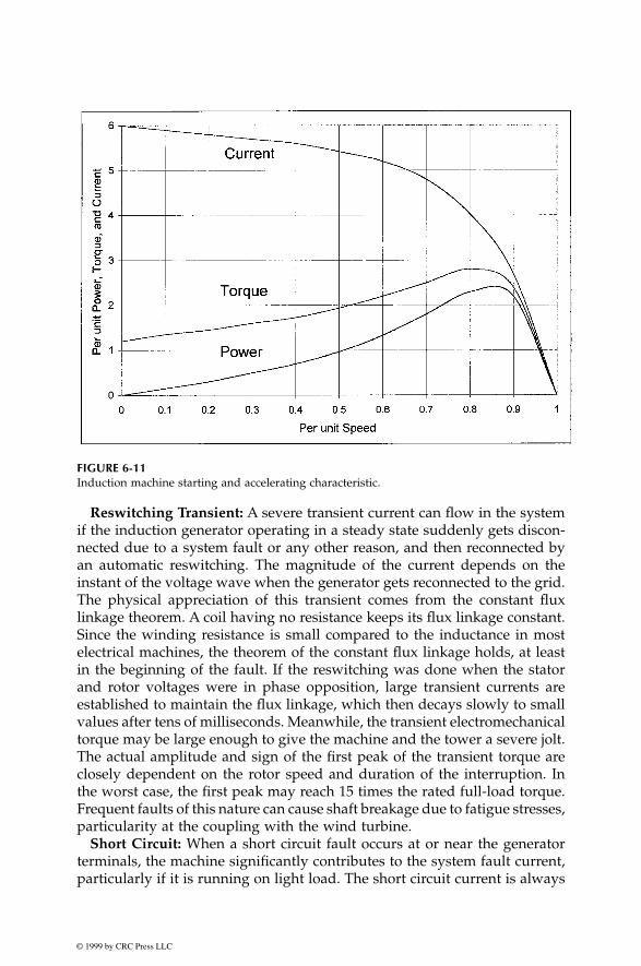
© 1999 by CRC Press LLC
Reswitching Transient:
A severe transient current can flow in the systemif the induction generator operating in a steady state suddenly gets discon-nected due to a system fault or any other reason, and then reconnected byan automatic reswitching. The magnitude of the current depends on theinstant of the voltage wave when the generator gets reconnected to the grid.The physical appreciation of this transient comes from the constant fluxlinkage theorem. A coil having no resistance keeps its flux linkage constant.Since the winding resistance is small compared to the inductance in mostelectrical machines, the theorem of the constant flux linkage holds, at leastin the beginning of the fault. If the reswitching was done when the statorand rotor voltages were in phase opposition, large transient currents areestablished to maintain the flux linkage, which then decays slowly to smallvalues after tens of milliseconds. Meanwhile, the transient electromechanicaltorque may be large enough to give the machine and the tower a severe jolt.The actual amplitude and sign of the first peak of the transient torque areclosely dependent on the rotor speed and duration of the interruption. Inthe worst case, the first peak may reach 15 times the rated full-load torque.Frequent faults of this nature can cause shaft breakage due to fatigue stresses,particularity at the coupling with the wind turbine.
Short Circuit:
When a short circuit fault occurs at or near the generatorterminals, the machine significantly contributes to the system fault current,particularly if it is running on light load. The short circuit current is always
FIGURE 6-11
Induction machine starting and accelerating characteristic.

© 1999 by CRC Press LLC
more severe for a single-phase fault than a three-phase fault. The mostimportant quantity is the first peak current as it determines the rating of theprotective circuit breaker needed to protect the generator against such faults.The short circuit current has a slowly decaying DC component, and an ACcomponent. The latter is larger than the direct on-line starting inrush current,and may reach 10-15 times the full load rated current.
The transient current and torque, in any case, are calculated using thegeneralized equivalent circuit of the machine in terms of the d-axis and q-axistransient and subtransient reactance and time constants.
4-6
The q-axis termsdo not enter in the induction generator transient analysis, as the d-axis andthe q-axis terms are identical due to the perfect circular symmetry in theelectromagnetic structure.
References
1. Rahim, Y. H. A. 1997. “Controlled Power Transfer from Wind Driven ReluctanceGenerators,” IEEE Winter Power Meeting, Paper No. PE-230-EC-1-09, New York,1997.
2. Say, M. G. 1983. “Alternating Current Machines,” New York, John Wiley &Sons, 1983.
3. Alger, P. L. 1965. “The Nature of Induction Machines.” New York, Gordon andBreach. 1965.
4. Adkins, B. 1964. “The General Theory of Electrical Machines,” London, Chap-man and Hall. 1964.
5. Kron, G. 1967. “Equivalent Circuits of Electrical Machines,” New York, DoverPublications, 1967.
6. Yamayee, Z. A. and Bala, J. L. 1994. “Electromechanical Devices and PowerSystems,” New York, John Wiley & Sons, 1994.

© 1999 by CRC Press LLC
7
Generator Drives
The turbine speed is generally much lower than the desired speed for theelectrical generator. For this reason, the turbine speed in most wind systemsis stepped up using a drive system. The system can be fixed-speed or vari-able-speed as described in this chapter.
The wind-power equation as derived in Chapter 3 is as follows:
(7-1)
where C
p
= rotor power coefficient.As seen earlier, the value of C
p
varies with the ratio of the rotor tip-speedto the wind speed, termed as the tip-speed-ratio TSR. Figure 7-1 depicts atypical relationship between the power coefficient and the tip-to-speed ratio.As the wind speed changes, the TSR and the power coefficient will vary. TheC
p
characteristic has single maximum at a specific value of the TSR. There-fore, when operating the rotor at constant speed, the power coefficient willbe maximum at only one wind speed.
For achieving the highest annual energy yield, the value of the rotor powercoefficient must be maintained at the maximum level all the time, regardlessof the wind speed. The theoretical maximum value of C
p
is 0.59, but thepractical limit is 0.5. Attaining C
p
above 0.4 is considered good. Whatevervalue is attainable with a given wind turbine, it must be maintained constantat that value. Therefore, the rotor speed must change in response to thechanging wind speed. To achieve this, the speed control must be incorpo-rated in the system design to run the rotor at high speed in high wind andat low speed in low wind. This is illustrated in Figure 7-2. For given windspeeds V
1
, V
2
,
or V
3
, the rotor power curves versus the turbine speed areplotted in solid lines. In order to extract the maximum possible energy overthe year, the turbine must be operated at the peak power point at all windspeeds. In the figure, this happens at points P
1
, P
2
, and P
3
for the wind speedV
1
, V
2
, and V
3
, respectively. The common factor among the peak powerproduction points P
1
, P
2
, and P
3
is the constant high value of TSR, close to 0.5.Operating the machine at the constant tip-speed ratio corresponding to
the peak power point means high rotor speed in gusty winds. The centrifugal
P AV Cp= ⋅12
3ρ

© 1999 by CRC Press LLC
forces produced in the rotor blades under such speeds can mechanicallydestroy the rotor. Moreover, the generator producing power above its ratedcapacity may electrically destroy the generator. For these reasons, the turbinespeed and the generator power output must be controlled.
7.1 Speed Control Regions
The speed and the power controls in the wind power systems have threedistinct regions:
• the optimum constant Cp region.• the speed-limited region.• the power-limited region.
These regions are shown in Figure 7-3. Typically the turbine starts operat-ing (cut in) when the wind speed exceeds 4-5 m/s, and is shut off at speedsexceeding 25 to 30 m/s. In between, it operates in one of the above regions.At a typical site, the wind-turbine may operate about 70 to 80 percent of thetime. Other times, it is off due to wind speed too low or too high.
FIGURE 7-1
Rotor power coefficient versus tip-speed ratio has a single maximum.
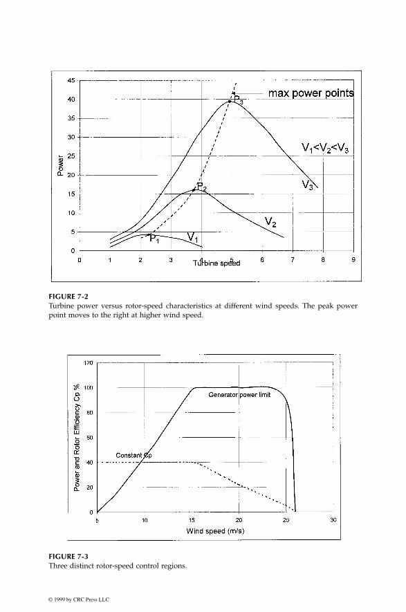
© 1999 by CRC Press LLC
FIGURE 7-2
Turbine power versus rotor-speed characteristics at different wind speeds. The peak powerpoint moves to the right at higher wind speed.
FIGURE 7-3
Three distinct rotor-speed control regions.
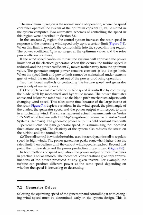
© 1999 by CRC Press LLC
The maximum C
p
region is the normal mode of operation, where the speedcontroller operates the system at the optimum constant C
p
value stored inthe system computer. Two alternative schemes of controlling the speed inthis region were described in Section 5.6.
In the constant C
p
region, the control system increases the rotor speed inresponse to the increasing wind speed only up to a certain limit (Figure 7-4).When this limit is reached, the control shifts into the speed-limiting region.The power coefficient C
p
is no longer at the optimum value, and the rotorpower efficiency suffers.
If the wind speed continues to rise, the systems will approach the powerlimitation of the electrical generator. When this occurs, the turbine speed isreduced, and the power coefficient C
p
moves farther away from the optimumvalue. The generator output power remains constant at the design limit.When the speed limit and power limit cannot be maintained under extremegust of wind, the machine is cut out of the power producing operation.
Two traditional methods of controlling the turbine speed and generatorpower output are as follows:
(1) The pitch control in which the turbine speed is controlled by controllingthe blade pitch by mechanical and hydraulic means. The power fluctuatesabove and below the rated value as the blade pitch mechanism adjusts withchanging wind speed. This takes some time because of the large inertia ofthe rotor. Figure 7-4 depicts variations in the wind speed, the pitch angle ofthe blades, the generator speed and the power output with respect to timein a fluctuating wind. The curves represent actual measurements on Vestas1.65 MW wind turbine with OptiSlip
®
(registered tradename of Vestas WindSystems, Denmark). The generator power output is held constant even with10 percent fluctuation in the generator speed, thus, minimizing the undesiredfluctuations on grid. The elasticity of the system also reduces the stress onthe turbine and the foundation.
(2) The stall control in which the turbine uses the aerodynamic stall to regulatespeed in high winds. The power generation peaks somewhat higher than therated limit, then declines until the cut-out wind speed is reached. Beyond thatpoint, the turbine stalls and the power production drops to zero (Figure 7-5).
In both methods of speed regulation, the power output of most machinesin practice is not as smooth. The theoretical considerations give only approx-imations of the power produced at any given instant. For example, theturbine can produce different power at the same speed depending onwhether the speed is increasing or decreasing.
7.2 Generator Drives
Selecting the operating speed of the generator and controlling it with chang-ing wind speed must be determined early in the system design. This is
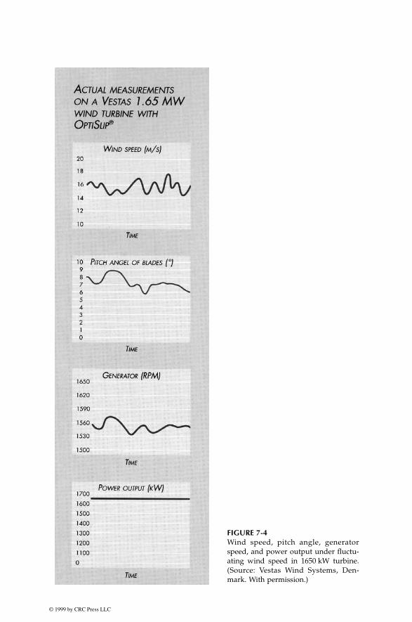
© 1999 by CRC Press LLC
FIGURE 7-4
Wind speed, pitch angle, generatorspeed, and power output under fluctu-ating wind speed in 1650 kW turbine.(Source: Vestas Wind Systems, Den-mark. With permission.)

© 1999 by CRC Press LLC
important, as it determines all major components and their ratings. Thealternative strategies and the corresponding speed control methods fall inthe following categories.
7.2.1 One Fixed-Speed Drive
The fixed-speed operation of the generator naturally fits well with the induc-tion generator, which is inherently a fixed-speed machine. However, theturbine speed is generally low, whereas the electrical generator works moreefficiently at high speed. The speed match between the two is accomplishedby the mechanical gear. The gearbox reduces the speed and increases thetorque, thus improving the rotor power coefficient C
p
. Under varying windspeed, the increase and decrease in electromagnetically converted torqueand power are accompanied by the corresponding increase or decrease inthe rotor slip with respect to the stator. The wind generator generally worksat 1 to 2 percent slip. The higher value benefits the drive gear, but increasesthe electrical loss in the rotor, which leads to cooling difficulty.
The annual energy yield for a fixed-speed wind turbine must be analyzedwith the given wind speed distribution at the site of interest. Since the speedis held constant, the turbine running above the rated speed is not a designconcern. However, it is possible to generate electrical power above the ratedcapacity of the generator. When this happens, the generator is shut off by
FIGURE 7-5
Generator output power variation with wind speed in the blade pitch-regulated and stall-regulated turbines.
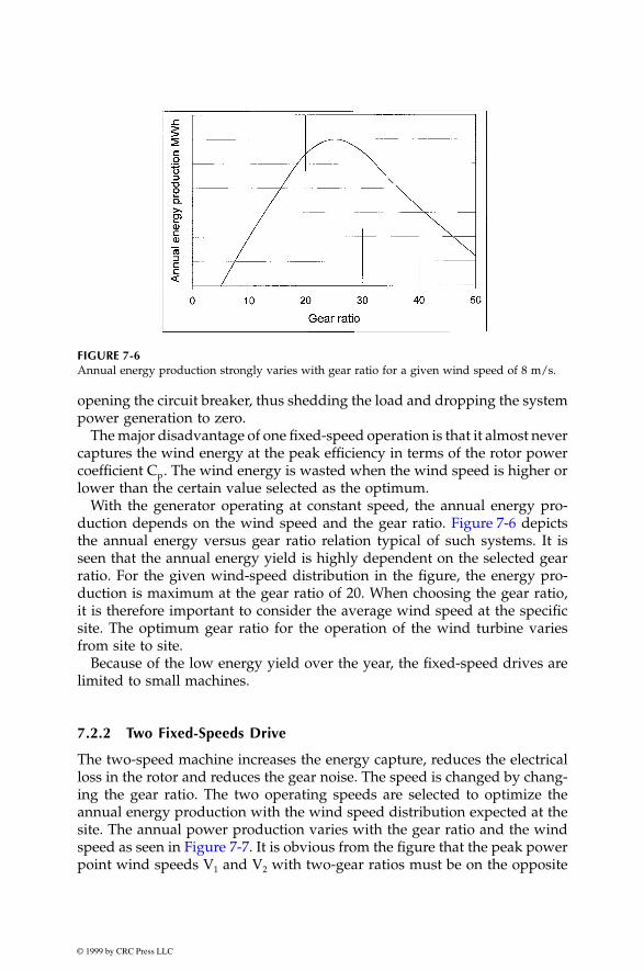
© 1999 by CRC Press LLC
opening the circuit breaker, thus shedding the load and dropping the systempower generation to zero.
The major disadvantage of one fixed-speed operation is that it almost nevercaptures the wind energy at the peak efficiency in terms of the rotor powercoefficient C
p
. The wind energy is wasted when the wind speed is higher orlower than the certain value selected as the optimum.
With the generator operating at constant speed, the annual energy pro-duction depends on the wind speed and the gear ratio. Figure 7-6 depictsthe annual energy versus gear ratio relation typical of such systems. It isseen that the annual energy yield is highly dependent on the selected gearratio. For the given wind-speed distribution in the figure, the energy pro-duction is maximum at the gear ratio of 20. When choosing the gear ratio,it is therefore important to consider the average wind speed at the specificsite. The optimum gear ratio for the operation of the wind turbine variesfrom site to site.
Because of the low energy yield over the year, the fixed-speed drives arelimited to small machines.
7.2.2 Two Fixed-Speeds Drive
The two-speed machine increases the energy capture, reduces the electricalloss in the rotor and reduces the gear noise. The speed is changed by chang-ing the gear ratio. The two operating speeds are selected to optimize theannual energy production with the wind speed distribution expected at thesite. The annual power production varies with the gear ratio and the windspeed as seen in Figure 7-7. It is obvious from the figure that the peak powerpoint wind speeds V
1
and V
2
with two-gear ratios must be on the opposite
FIGURE 7-6
Annual energy production strongly varies with gear ratio for a given wind speed of 8 m/s.

© 1999 by CRC Press LLC
side of the expected annual average wind speed. For the specific exampleof Figure 7-7, the system is operated on the low-gear ratio for wind speedbelow 10 m/s, and on the high-gear ratio for wind speed above 10 m/s. Thegear ratio is changed at 10 m/s in this example.
In some early American designs, two speeds were achieved by using twoseparate generators and switching between the generators by a belt drive.
An economic and efficient method is to design the induction generator tooperate at two speeds. The cage motor with two separate stator windingsof different pole numbers can run at two or more integrally related speeds.The pole-changing motor, on the other hand, has a single winding, theconnection of which is changed to give different numbers of poles. Separatewindings matching with the system requirement may be preferred wherethe speed change must be made without losing control of the machine.Separate windings are, however, difficult to accommodate.
In the pole-changing method with one winding, the stator is wound withcoils that can be connected either in P or 2P number of poles. No changesare needed, nor possible, in the squirrel cage rotor. The stator connectionwhich produces a higher pole number for low-speed operation is changedto one-half as many poles for high-speed operation. This maintains the tip-speed ratio near the optimum to produce high rotor power coefficient C
p
.The machine, however, operates with only one-speed ratio of 2:1.
Figure 7-8 shows one phase of the pole changing stator winding. For thehigher pole number, the coils are in series. For the lower number, they arein series-parallel. The resulting magnetic flux pattern corresponds to eightand four poles, respectively. It is common to use double layer winding, with120° electrical span for the higher pole number. An important design
FIGURE 7-7
Power production probability distribution with wind speed with low and high gear ratios.
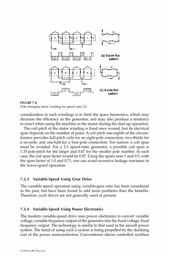
© 1999 by CRC Press LLC
consideration in such windings is to limit the space harmonics, which maydecrease the efficiency as the generator, and may also produce a tendencyto crawl when using the machine as the motor during the start up operation.
The coil pitch of the stator winding is fixed once wound, but its electricalspan depends on the number of poles. A coil pitch one-eighth of the circum-ference provides full-pitch coils for an eight-pole connection, two-thirds fora six-pole, and one-half for a four-pole connection. Too narrow a coil spanmust be avoided. For a 2:1 speed-ratio generator, a possible coil span is1.33 pole-pitch for the larger and 0.67 for the smaller pole number. In eachcase, the coil span factor would be 0.87. Using the spans near 1 and 0.5, withthe span factor of 1.0 and 0.71, one can avoid excessive leakage reactance inthe lower-speed operation.
7.2.3 Variable-Speed Using Gear Drive
The variable-speed operation using variable-gear ratio has been consideredin the past, but have been found to add more problems than the benefits.Therefore, such drives are not generally used at present.
7.2.4 Variable-Speed Using Power Electronics
The modern variable-speed drive uses power electronics to convert variablevoltage, variable frequency output of the generator into the fixed voltage, fixedfrequency output. The technology is similar to that used in the aircraft powersystem. The trend of using such a system is being propelled by the decliningcost of the power semiconductors. Conventional silicon controlled rectifiers
FIGURE 7-8
Pole-changing stator winding for speed ratio 2:1.

© 1999 by CRC Press LLC
and inverters can be used, but the modern design in the wind industry appearsto prefer pulse-width-modulated thyristors. The speed ratio is not limitedin theory, but practical considerations limit the ratio to 3:1, which is widerthan that obtainable using the pole-changing method described above andthe Scherbius machine described later. The energy yield of the variable-speedsystem is higher. However, the added cost and the electrical loss in the powerelectronics partially offset the benefit. The cost and benefit trade is generallypositive for large machines.
The power-electronics based variable-speed system introduces some sys-tem level issues not found in other systems. It produces high-frequencyharmonics (electrical noise) in the network, which degrades the quality ofpower. Alternatively, for the same quality of power, it requires a higherdegree of electrical filtering to meet the grid-quality requirement.
In addition to high annual energy production, the variable-speed powerelectronic system offers remotely adjustable and controllable quality ofpower. This has two major benefits not available in other systems:
• opportunity for remote control. This makes it attractive for offshoreapplications.
• fine-tuning for superior grid connection, making it better suited for meeting the demand of weak grids in developing countries like China and India.
7.2.5 Scherbius Variable-Speed Drive
Compared to the variable-speed system using power electronics, the Scher-bius machine offers lower cost and eliminates the power quality disadvan-tage. It has been used in hoist applications in factories and mines. Extendingthe analysis of the equivalent circuit described in Chapter 6, the speed of theinduction machine can be changed by changing the rotor resistance or byinjecting an external voltage of the frequency corresponding to the desiredrotor slip. The squirrel cage construction does not allow such injection.Therefore, the wound rotor construction with slip rings is used (Figure 7-9).The rotor circuit is connected to an external variable frequency source viaslip rings, and the stator is connected to the grid system. For this reason, theScherbius machine is also called the doubly-fed induction machine. It is fedfrom both the stator and the rotor. The speed is controlled by adjusting thefrequency of the external source of the rotor current. The range of variable-speed control using the Scherbius machines is generally limited to 2:1.
The concept was used in early turbines. The decreased reliability due tothe rubbing electrical contacts at the slip rings had been a concern. However,some manufacturers appear to have resolved this concern, and are imple-menting the system in turbines with several hundred kW ratings. The needof the variable frequency source for the rotor adds into the cost and com-plexity. For large systems, however, the added cost may be less than thebenefit of greater energy production of the variable-speed operation.

© 1999 by CRC Press LLC
7.2.6 Variable-Speed Direct Drive
The generator that operates directly at the turbine speed is extremely attrac-tive. This is possible particularity for small machines where the rotor speedis high. The direct drive eliminates the mechanical gear altogether, and needsno power electronics. This results in multiple benefits:
• lower nacelle weight.• reduced noise and vibration.• lower power loss by several percent.• less frequent servicing requirement at the nacelle.
The last benefit is particularly attractive for offshore installation.The low rotor-speed requirement for large rotors imposes a design lim-
itation on the electrical machine. That is, the generator must have largenumbers of poles. Such machines must have short pole-pitch, resulting inpoor magnetic design. To circumvent such limitation, the permanent mag-net and wound rotor synchronous machines are being considered for1.5 MW direct drive generators. Another possible solution is the axial gapinduction machine. It can be designed with a large number of poles withless difficulty compared to the conventional radial gap induction machine.The axial gap machine is being considered for direct drive marine propul-sion, which is inherently a low-speed system. For small gearless winddrives, the axial-flux permanent magnet generator may find some interestfor its simplicity. A 5 kW, 200 revolution-per-minute laboratory prototypeof the axial-gap permanent magnet design has been recently tested,
1
how-ever, significant research and development effort is needed before the vari-able-speed direct drive systems can be commercially made available forlarge wind power systems.
FIGURE 7-9
Scherbius adjustable-speed drive system injects variable frequency voltage in the wound rotorcircuit.

© 1999 by CRC Press LLC
7.3 Drive Selection
The variable-speed operation can capture theoretically about one-third moreenergy per year than the fixed-speed system.
2
The actual improvementreported by the variable-speed systems operators in the field is lower, around20 to 35 percent. However, the improvement of even 15 to 20 percent in theannual energy yield by variable-speed operation can make the systems com-mercially viable in low wind region. This can open a whole new market forthe wind-power installations, and this is happening at present in manycountries. Therefore the newer installations are more likely to use the vari-able-speed systems.
As of 1997, the distribution of the system design is 35 percent one fixed-speed, 45 percent two fixed-speed and 20 percent variable-speed power elec-tronics systems (Figure 7-10). The market share of the variable-speed sys-tems, however, is increasing every year.
3
7.4 Cut-Out Speed Selection
In any case, it is important that the machine is operated below its speed andpower limits. Exceeding either one above the design limit can damage andeven destroy the machine.
FIGURE 7-10
Design choices in generator drive systems.

© 1999 by CRC Press LLC
In designing the variable-speed system, important decision must be madeon the upper limit of the operating speed. For the energy distribution shownin Figure 7-11, if the wind plant is designed to operate at fixed speed V
1
, itcan capture energy E
1
over the year. On the other hand, if it is designed tooperate at a variable speed up to V
2
, it can capture energy E
2
over the sameperiod. The latter, however, comes with an added cost of designing the windturbine and the generator to handle high power. The benefit and cost mustbe traded-off for the given site to arrive at the optimum upper limit on therotor speed.
On one side of the trade is additional energy (E
2
– E
1
) that can be capturedover the year. If the revenue of the generated electricity is valued at p $/kWh,the added benefit per year is p · (E
2
– E
1
) dollars. The present worth
P
of thisyearly benefit over the life of
n
years at the annual cost of capital
i
is as follows:
(7-2)
If the variable-speed system requires additional capital cost of C, then thevariable-speed system will be financially beneficial if C < P.
FIGURE 7-11
Probability distribution of annual energy production at various cut out speeds.
P p E Ei
i i
n
n= ⋅ −( ) +( ) −+( )
2 1
1 11

© 1999 by CRC Press LLC
References
1. Chalmers, B. J. and Spooner, E. 1998. “Axial flux permanent magnet generatorfor gearless wind energy systems,”
IEEE Paper No. PE-P13-EC-02,
July 1998.2. Zinger, D. S., Muljadi, E. 1997. “Annualized wind energy improvement using
variable-speed,”
IEEE Transactions on Industry Applications,
Vol. 33-6, p. 1444-47,1997.
3. Gardner, P. 1997. “Wind turbine generator and drive systems,”
Wind Directions,Magazine of the European Wind Energy Association,
London, October, 1997.

© 1999 by CRC Press LLC
8
Solar Photovoltaic Power System
The photovoltaic effect is the electrical potential developed between twodissimilar materials when their common junction is illuminated with radia-tion of photons. The photovoltaic cell, thus, converts light directly into elec-tricity. The pv effect was discovered in 1839 by French physicist Becquerel. Itremained in the laboratory until 1954, when Bell Laboratories produced thefirst silicon solar cell. It soon found application in the U.S. space programsfor its high power capacity per unit weight. Since then it has been an impor-tant source of power for satellites. Having developed maturity in the spaceapplications, the pv technology is now spreading into the terrestrial applica-tions ranging from powering remote sites to feeding the utility lines.
8.1 The pv Cell
The physics of the pv cell is very similar to the classical p-n junction diode(Figure 8-1). When light is absorbed by the junction, the energy of theabsorbed photons is transferred to the electron system of the material, result-ing in the creation of charge carriers that are separated at the junction. Thecharge carriers may be electron-ion pairs in a liquid electrolyte, or electron-hole pairs in a solid semiconducting material. The charge carriers in thejunction region create a potential gradient, get accelerated under the electricfield and circulate as the current through an external circuit. The currentsquared times the resistance of the circuit is the power converted into elec-tricity. The remaining power of the photon elevates the temperature of the cell.
The origin of the photovoltaic potential is the difference in the chemicalpotential, called the Fermi level, of the electrons in the two isolated materials.When they are joined, the junction approaches a new thermodynamic equi-librium. Such equilibrium can be achieved only when the Fermi level is equalin the two materials. This occurs by the flow of electrons from one materialto the other until a voltage difference is established between the two mate-rials which have the potential just equal to the initial difference of the Fermilevel. This potential drives the photocurrent.

© 1999 by CRC Press LLC
Figure 8-2 shows the basic cell construction.
1
For collecting the photocur-rent, the metallic contacts are provided on both sides of the junction to collectelectrical current induced by the impinging photons on one side. Conductingfoil (solder) contact is provided over the bottom (dark) surface and on oneedge of the top (illuminated) surface. Thin conducting mesh on the remain-ing top surface collects the current and lets the light through. The spacingof the conducting fibers in the mesh is a matter of compromise betweenmaximizing the electrical conductance and minimizing the blockage of thelight. In addition to the basic elements, several enhancement features arealso included in the construction. For example, the front face of the cell hasanti-reflective coating to absorb as much light as possible by minimizing thereflection. The mechanical protection is provided by the coverglass appliedwith a transparent adhesive.
FIGURE 8-1
Photovoltaic effect converts the photon energy into voltage across the p-n junction.
FIGURE 8-2
Basic construction of pv cell with performance enhancing features (current collecting mesh,anti-reflective coating and cover glass protection).

© 1999 by CRC Press LLC
8.2 Module and Array
The solar cell described above is the basic building block of the pv powersystem. Typically, it is a few square inches in size and produces about onewatt of power. For obtaining high power, numerous such cells are connectedin series and parallel circuits on a panel (module) area of several square feet(Figure 8-3). The solar array or panel is defined as a group of several moduleselectrically connected in series-parallel combinations to generate therequired current and voltage. Figure 8-4 shows the actual construction of amodule in a frame that can be mounted on a structure.
Mounting of the modules can be in various configurations as seen inFigure 8-5. In the roof mounting, the modules are in the form that can belaid directly on the roof. In the newly developed amorphous silicon technol-ogy, the pv sheets are made in shingles that can replace the traditional roofshingles on one-to-one basis, providing a better economy in the material andlabor.
8.3 Equivalent Electrical Circuit
The complex physics of the pv cell can be represented by the equivalentelectrical circuit shown in Figure 8-6. The circuit parameters are as follows.
FIGURE 8-3
Several pv cells make a module and several modules make an array.

© 1999 by CRC Press LLC
The output-terminal current I is equal to the light-generated current I
L
, lessthe diode-current I
d
and the shunt-leakage current I
sh
. The series resistanceR
s
represents the internal resistance to the current flow, and depends on thep-n junction depth, the impurities and the contact resistance. The shuntresistance R
sh
is inversely related with leakage current to the ground. In anideal pv cell, R
s
= 0 (no series loss), and R
sh
=
∞
(no leakage to ground). Ina typical high quality one square inch silicon cell, R
s
= 0.05 to 0.10 ohm andR
sh
= 200 to 300 ohms. The pv conversion efficiency is sensitive to smallvariations in R
s
, but is insensitive to variations in R
sh
. A small increase in R
s
can decrease the pv output significantly.In the equivalent circuit, the current delivered to the external load equals
the current I
L
generated by the illumination, less the diode current I
d
andthe ground-shunt current I
sh
. The open circuit voltage V
oc
of the cell isobtained when the load current is zero, i.e., when I = 0, and is given by thefollowing:
FIGURE 8-4
Construction of pv module: 1) frame, 2) weatherproof junction box, 3) rating plate, 4) weatherprotection for 30-year life, 5) pv cell, 6) tempered high transmissivity coverglass, 7) outsideelectrical bus, 8) frame clearance. (Source: Solarex Corporation, Frederick, Maryland, Withpermission.)
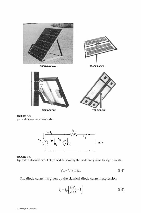
© 1999 by CRC Press LLC
V
oc
= V + I R
sh
(8-1)
The diode current is given by the classical diode current expression:
(8-2)
FIGURE 8-5
pv module mounting methods.
FIGURE 8-6
Equivalent electrical circuit of pv module, showing the diode and ground leakage currents.
I IQVAKTd D
oc= −
1

© 1999 by CRC Press LLC
where I
D
= the saturation current of the diodeQ = electron charge = 1.6 · 10
–19
CoulombsA = curve fitting constantK = Boltzmann constant = 1.38 · 10
–23
Joule/°KT = temperature on absolute scale °K
The load current is therefore given by the expression:
(8-3)
The last term, the ground-leakage current, in practical cells is small com-pared to I
L
and I
D
, and can be ignored. The diode-saturation current can,therefore, be determined experimentally by applying voltage V
oc
in the darkand measuring the current going into the cell. This current is often calledthe dark current or the reverse diode-saturation current.
8.4 Open Circuit Voltage and Short Circuit Current
The two most important parameters widely used for describing the cellelectrical performance is the open-circuit voltage V
oc
and the short-circuitcurrent I
sc
. The short-circuit current is measured by shorting the outputterminals, and measuring the terminal current under full illumination. Ignor-ing the small diode and the ground-leakage currents under zero-terminalvoltage, the short-circuit current under this condition is the photocurrent I
L
.The maximum photovoltage is produced under the open-circuit voltage.
Again, by ignoring the ground-leakage current, Equation 8-3 with I = 0 givesthe open-circuit voltage as the following:
(8-4)
The constant KT/Q is the absolute temperature expressed in voltage(300°K = 0.026 volt). In practical photocells, the photocurrent is severalorders of magnitude greater than the reverse saturation current. Therefore,the open-circuit voltage is many times the KT/Q value. Under condition ofconstant illumination, I
L
/I
D
is a sufficiently strong function of the cell tem-perature, and the solar cell ordinarily shows a negative temperature coeffi-cient of the open-circuit voltage.
I I I eVocRL D
QVAKT
sh
oc
= − −
−1
VAKT
QLog
IIoc n
L
D
= +
1

© 1999 by CRC Press LLC
8.5 i-v and p-v Curves
The electrical characteristic of the pv cell is generally represented by thecurrent versus voltage (i-v) curve. Figure 8-7 shows the i-v characteristic ofa pv module under two conditions, in sunlight and in dark. In the firstquadrant, the top left of the i-v curve at zero voltage is called the short-circuit current. This is the current we would measure with the output ter-minals shorted (zero voltage). The bottom right of the curve at zero currentis called the open-circuit voltage. This is the voltage we would measure withthe output terminals open (zero current). In the left shaded region, the cellworks like a constant current source, generating voltage to match with theload resistance. In the shaded region on the right, the current drops rapidlywith a small rise in voltage. In this region, the cell works like a constantvoltage source with an internal resistance. Somewhere in the middle of thetwo shaded regions, the curve has a knee point.
If the voltage is externally applied in the reverse direction, say during asystem fault transient, the current remains flat and the power is absorbedby the cell. However, beyond a certain negative voltage, the junction breaksdown as in a diode, and the current rises to a high value. In the dark, thecurrent is zero for voltage up to the breakdown voltage which is the sameas in the illuminated condition.
The power output of the panel is the product of the voltage and the currentoutputs. In Figure 8-8, the power is plotted against the voltage. Notice that
FIGURE 8-7
Current versus voltage (i-v) characteristics of the pv module in sunlight and in dark.
FIGURE 8-8
Power versus voltage (p-v) character-istics of the pv module in sunlight.

© 1999 by CRC Press LLC
the cell produces no power at zero voltage or zero current, and producesthe maximum power at voltage corresponding to the knee point of the i-vcurve. This is why pv power circuits are designed such that the modulesoperate closed to the knee point, slightly on the left hand side. The pvmodules are modeled approximately as a constant current source in theelectrical analysis of the system.
Figure 8-9 is the i-v characteristic of a 22-watts panel under two solarillumination intensities, 1,000 watts/m
2
and 500 watts/m
2
. These curves areat AM1.5 (air mass 1.5). The air mass zero (AM0) represents the conditionin outer space, where the solar radiation is 1,350 watts/m
2
. The AM1 repre-sents the ideal earth condition in pure air on a clear dry noon when thesunlight experiences the least resistance to reach earth. The air we find on atypical day with average humidity and pollution is AM1.5, which is takenas the reference value. The solar power impinging a normal surface on abright day with AM1.5 is about 1,000 watts/m
2
. On a cloudy day, it wouldbe low. The 500 watts/m
2
solar intensity is another reference condition theindustry uses to report the i-v curves.
The photoconversion efficiency of the pv cell is defined as the following:
(8-5)
Obviously, the higher the efficiency, the higher the output power we getunder a given illumination.
8.6 Array Design
The major factors influencing the electrical design of the solar array are asfollows:
• the sun intensity.• the sun angle.• the load matching for maximum power.• the operating temperature.
These factors are discussed below.
8.6.1 Sun Intensity
The magnitude of the photocurrent is maximum under full bright sun (1.0 sun).On a partially sunny day, the photocurrent diminishes in direct proportion tothe sun intensity. The i-v characteristic shifts downward at a lower sun
η = electrical power outputsolar power impinging the cell

© 1999 by CRC Press LLC
FIGURE 8-9
i-v characteristic of 22 watts pv module at full and half sun intensities. (Source: United SolarSystems Corporation, San Diego, California. With permission.)

© 1999 by CRC Press LLC
intensity as shown in Figure 8-10. On a cloudy day, therefore, the short circuitcurrent decreases significantly. The reduction in the open-circuit voltage,however, is small.
The photoconversion efficiency of the cell is insensitive to the solar radi-ation in the practical working range. For example, Figure 8-11 shows thatthe efficiency is practically the same at 500 watts/m
2
and 1,000 watts/m
2
.This means that the conversion efficiency is the same on a bright sunny dayand a cloudy day. We get lower power output on a cloudy day only becauseof the lower solar energy impinging the cell.
8.6.2 Sun Angle
The cell output current is given by
I
=
I
0
cos
θ
, where I
o
is the current withnormal sun (reference), and
θ
is the angle of the sunline measured from thenormal. This cosine law holds well for sun angles ranging from 0 to about 50°.
FIGURE 8-10
i-v characteristic of pv module shifts down at lower sun intensity, with small reduction involtage.
FIGURE 8-11
Photoconversion efficiency versus solar radiation. The efficiency is practically constant over awide range of radiation.

© 1999 by CRC Press LLC
Beyond 50°, the electrical output deviates significantly from the cosine law,and the cell generates no power beyond 85°, although the mathematical cosinelaw predicts 7.5 percent power generation. The actual power-angle curve ofthe pv cell is called Kelly cosine, and is shown in Figure 8-12 and Table 8-1.
8.6.3 Shadow Effect
The array may consist of many parallel strings of series-connected cells. Twosuch strings are shown in Figure 8-13. A large array may get partially shad-owed due to a structure interfering with the sunline. If a cell in a long-seriesstring gets completely shadowed, it will lose the photovoltage, but still mustcarry the string current by virtue of its being in series with the other fullyoperating cells. Without internally generated voltage, it cannot producepower. Instead, it acts as a load, producing local I
2
R loss and heat. Theremaining cells in the string must work at higher voltage to make up theloss of the shadowed cell voltage. Higher voltage in healthy cells meanslower string current as per the i-v characteristic of the string. This is shownin the bottom left of Figure 8-13. The current loss is not proportional to theshadowed area, and may go unnoticed for mild shadow on a small area.However, if more cells are shadowed beyond the critical limit, the i-v curve
FIGURE 8-12
Kelley cosine curve for pv cell at sun angles from 0 to 90°.
TABLE 8-1
The Kelley Cosine Values of the Photocurrent
in Silicon Cells
Sun AngleDegrees
MathematicalCosine Value
KellyCosine Value
30 0.866 0.86650 0.643 0.63560 0.500 0.45080 0.174 0.10085 0.087 0

© 1999 by CRC Press LLC
gets below operating voltage of the string, making the string current fall tozero, losing all power of the string.
The commonly used method to eliminate the loss of string due to shadoweffect is to subdivide the circuit length in several segments with bypassdiodes (Figure 8-14). The diode across the shadowed segment bypasses onlythat segment of the string. This causes a proportionate loss of the stringvoltage and current, without losing the whole string power. Some modernpv modules come with such internally embedded bypass diodes.
FIGURE 8-13
Shadow effect on one long pv string of an array. The power degradation is small until shadowexceeds the critical limit.
FIGURE 8-14
Bypass diode in pv string minimizes the power loss under heavy shadow.
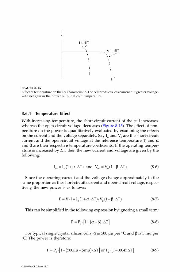
© 1999 by CRC Press LLC
8.6.4 Temperature Effect
With increasing temperature, the short-circuit current of the cell increases,whereas the open-circuit voltage decreases (Figure 8-15). The effect of tem-perature on the power is quantitatively evaluated by examining the effectson the current and the voltage separately. Say I
o
and V
o
are the short-circuitcurrent and the open-circuit voltage at the reference temperature T, and
α
and
β
are their respective temperature coefficients. If the operating temper-ature is increased by
∆
Τ
, then the new current and voltage are given by thefollowing:
(8-6)
Since the operating current and the voltage change approximately in thesame proportion as the short-circuit current and open-circuit voltage, respec-tively, the new power is as follows:
(8-7)
This can be simplified in the following expression by ignoring a small term:
(8-8)
For typical single crystal silicon cells,
α
is 500 µu per °C and
β
is 5 mu per°C. The power is therefore:
(8-9)
FIGURE 8-15
Effect of temperature on the i-v characteristic. The cell produces less current but greater voltage,with net gain in the power output at cold temperature.
I I T and V V Tsc o oc o= + ⋅( ) = − ⋅( )1 1α β∆ ∆
P V I I T V To o= ⋅ = + ⋅( ) ⋅ − ⋅( )1 1α β∆ ∆
P P To= ⋅ + −( ) ⋅[ ]1 α β ∆
P P u mu T or P To o= ⋅ + µ −( ) ⋅[ ] ⋅ −[ ]1 500 5 1 0045∆ ∆.

© 1999 by CRC Press LLC
This expression indicates that for every °C rise in the operating tempera-ture above the reference temperature, the silicon cell power output decreasesby 0.45 percent. Since the increase in the current is much less than thedecrease in the voltage, the net effect is the decrease in power at highoperating temperatures.
The effect of varying temperature on the power output is shown in thepower versus voltage characteristics at two operating temperatures inFigure 8-16. The figure shows that the maximum power available at lowertemperature is higher than that at higher temperature. Thus, cold tempera-ture is actually better for the pv cell, as it generates more power. However,the two P
max
points are not at the same voltage. In order to extract maximumpower at all temperatures, the pv system must be designed such that themodule output voltage can increase to V
2
for capturing P
max2
at lower tem-perature and can decrease to V
1
for capturing P
max1
at higher temperature.
8.6.5 Effect of Climate
On a partly cloudy day, the pv module can produce up to 80 percent of theirfull sun power. Even on an extremely overcast day, it can produce about30 percent power. Snow does not usually collect on the modules, becausethey are angled to catch the sun. If snow does collect, it quickly melts.Mechanically, modules are designed to withstand golf ball size hail.
8.6.6 Electrical Load Matching
The operating point of any power system is the intersection of the sourceline and the load line. If the pv source having the i-v and p-v characteristics
FIGURE 8-16
Effect of temperature on the p-v characteristic. The cell produces more power at cold temperature.

© 1999 by CRC Press LLC
shown in Figure 8-17 (a) is supplying the power to the resistive load R
1
, itwill operate at point A
1
. If the load resistance increases to R
2
or R
3
, theoperating point moves to A
2
or A
3
, respectively. The maximum power isextracted from the module when the load resistance is R
2
(Figure 8-17b).Such load matching with the source is always necessary for maximum powerextraction from the pv module.
The operation with constant power loads is shown in Figure 8-17(c) and(d). The constant power load line has two points of intersection with thesource line, denoted by B
1
and B
2
. Only point B
2
is stable, as any perturbationfrom it will generate a restoring power to take the operation back to B
2
.Therefore, the system will operate at B
2
.The necessary condition for the electrical operating stability of the solar
array is as follows:
(8-10)
Some loads such as heaters have constant resistance, with power varyingwith the voltage squared. On the other hand, some loads such as inductionmotors behave more like constant power loads, drawing more current atlower voltage. In most large systems with mix loads, the power variesapproximately in linear proportion with voltage.
8.6.7 Sun Tracking
More energy is collected by the end of the day if the pv module is installedon a tracker, with an actuator that follows the sun like a sunflower. Thereare two types of sun trackers:
FIGURE 8-17
Operating stability and electrical load matching with resistive load and constant power load.
dPdV
dPdVload source
>
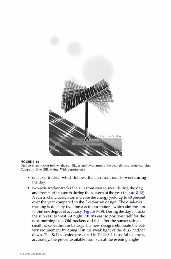
© 1999 by CRC Press LLC
• one-axis tracker, which follows the sun from east to west duringthe day.
• two-axis tracker tracks the sun from east to west during the day, and from north to south during the seasons of the year (Figure 8-18). A sun tracking design can increase the energy yield up to 40 percent over the year compared to the fixed-array design. The dual-axis tracking is done by two linear actuator motors, which aim the sun within one degree of accuracy (Figure 8-19). During the day, it tracks the sun east to west. At night it turns east to position itself for the next morning sun. Old trackers did this after the sunset using a small nickel-cadmium battery. The new designs eliminate the bat-tery requirement by doing it in the weak light of the dusk and/or dawn. The Kelley cosine presented in Table 8-1 is useful to assess, accurately, the power available from sun at the evening angles.
FIGURE 8-18
Dual-axis suntracker follows the sun like a sunflower around the year. (Source: American SunCompany, Blue Hill, Maine. With permission.)
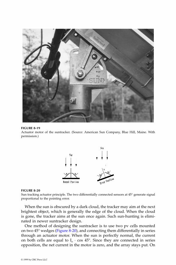
© 1999 by CRC Press LLC
When the sun is obscured by a dark cloud, the tracker may aim at the nextbrightest object, which is generally the edge of the cloud. When the cloudis gone, the tracker aims at the sun once again. Such sun-hunting is elimi-nated in newer suntracker design.
One method of designing the suntracker is to use two pv cells mountedon two 45° wedges (Figure 8-20), and connecting them differentially in seriesthrough an actuator motor. When the sun is perfectly normal, the currenton both cells are equal to I
o
· cos 45°. Since they are connected in seriesopposition, the net current in the motor is zero, and the array stays put. On
FIGURE 8-19
Actuator motor of the suntracker. (Source: American Sun Company, Blue Hill, Maine. Withpermission.)
FIGURE 8-20
Sun tracking actuator principle. The two differentially connected sensors at 45° generate signalproportional to the pointing error.

© 1999 by CRC Press LLC
the other hand, if the array is not normal to the sun, the sun angles on thetwo cells are different, giving two different currents:
The motor current is therefore:
Using Taylor series expansion:
we can express the two currents as the following:
The motor current is then (8-11)
Small pole-mounted panels can use one pole-mounted suntracker. Largearray, on the other hand, is divided into small modules, each mounted onits own single-axis or dual-axis tracker. This simplifies the structure andeliminates the problems related with large motion.
8.7 Peak Power Point Operation
The suntracker drives the module mechanically to face the sun to collect themaximum solar radiation. However, that, in itself, does not guarantee themaximum power output from the module. As was seen in Figure 8-16, themodule must operate electrically at a certain voltage which corresponds tothe peak power point under the given operating conditions. First we examinethe electrical principle of the peak power operation.
If the array is operating at voltage V and current I on the i-v curve, thepower generation is P = V · I watts. If the operation moves away from theabove point, such that the current is now I +
∆
I, and the voltage is V +
∆
V,the new power is as follows:
I I , and I Io 2 o1 45 45= +( ) = −( )cos cosδ δ
I I I I Im 1 2 o o= − = +( ) − −( )cos cos45 45δ δ
f x h f x h f xh
f x+( ) = ( ) + ⋅ ′( ) + ′′( ) +2
2!L
I I I , and
I I I
o o
o o
1
2
45 45
45 45
= −
= −
cos sin
cos sin
δ
δ
I I I I
I if is in radian
m o
o
= − = °
=
1 2 2 45
2
δ
δ δ
sin
© 1999 by CRC Press LLC
(8-12)
Which, after ignoring a small term, simplifies to the following:
(8-13)
The
∆
P should be zero at peak power point, which necessarily lies on alocally flat neighborhood. Therefore, at peak power point, the above expres-sion in the limit becomes as follows:
(8-14)
We take note here that dV/dI is the dynamic impedance of the source, andV/I is the static impedance.
There are three electrical methods of extracting the peak power from themodule, as described below:
(1) In the first method, a small signal current is periodically injected intothe array bus and the dynamic bus impedance Z
d
= dV/dI and the static busimpedance Z
s
= V/I are measured. The operating voltage is then increasedor decreased until Z
d
= – Z
s
. At this point, the maximum power is extractedfrom the source.
(2) In another electrical method, the operating voltage is increased as longas dP/dV is positive. That is, the voltage is increased as long as we get morepower. If dP/dV is sensed negative, the operating voltage is decreased. Thevoltage is kept put if the dP/dV is near zero within a preset dead band.
(3) The third method makes use of the fact that for most pv cells, the ratioof the voltage at the maximum power point to the open circuit voltage (i.e.,V
mp
/V
oc
) is approximately constant, say K. For example, for high-qualitycrystalline silicon cells K = 0.72. An unloaded cell is installed on the arrayand kept in the same environment as the power-producing module, and itsopen circuit voltage is continuously measured. The operating voltage of thepower-producing array is then set at K·V
oc
, which will produce the maximumpower.
8.8 pv System Components
The array by itself does not constitute the pv power system. We must alsohave a structure to mount it, point to the sun, and the components that acceptthe DC power produced by the array and condition the power in the formthat is usable by the load. If the load is AC, the system needs an inverter toconvert the DC power into AC, generally at 50 or 60 Hz.
P P V V I I+ = +( ) ⋅ +( )∆ ∆ ∆
∆ ∆ ∆P V I + I V= ⋅ ⋅
dVdI
VI
= −

© 1999 by CRC Press LLC
Figure 8-21 shows the necessary components of a stand-alone pv powersystem. The peak power tracker senses the voltage and current outputs ofthe array and continuously adjusts the operating point to extract the maxi-mum power under the given climatic conditions. The output of the arraygoes to the inverter, which converts the DC into AC. The array output inexcess of the load requirement is used to charge the battery. The batterycharger is usually a DC-DC buck converter. If excess power is still availableafter fully charging the battery, it is shunted in dump heaters, which may bespace or room heaters in a stand-alone system. When the sun is not available,the battery discharges to the inverter to power the loads. The battery dis-charge diode Db is to prevent the battery from being charged when thecharger is opened after a full charge or for other reasons. The array diode Dais to isolate the array from the battery, thus keeping the array from acting asload on the battery at night. The mode controller collects the system signals,such as the array and the battery currents and voltages, keeps track of thebattery state of charge by bookkeeping the charge/discharge ampere-hours,and commands the charger, discharge converter, and dump heaters on or offas needed. The mode controller is the central controller for the entire system.
In the grid-connected system, dump heaters are not required, as all excesspower is fed to the grid lines. The battery is also eliminated, except for smallcritical loads, such as the start up controls and the computers. The DC poweris first converted into AC by the inverter, ripples are filtered and then onlythe filtered power is fed into the grid lines.
For pv applications, the inverter is a critical component, which convertsthe array DC power into AC for supplying the loads or interfacing with thegrid. A new product recently being introduced into the market is the AC-pvmodules, which integrates an inverter directly in the module, and is pres-ently available in a few hundred watts capacity. It provides utility grade60 Hz power directly from the module junction box. This greatly simplifiesthe pv system design.
FIGURE 8-21Peak power tracking photovoltaic power system showing major components.

© 1999 by CRC Press LLC
References
1. Cook, G., Billman, L. and Adcock R. 1995. “Photovoltaic Fundamental,”DOE/Solar Energy Research Institute Report No. DE91015001, February 1995.

0-8493-????-?/97/$0.00+$.50© 1997 by CRC Press LLC
© 1999 by CRC Press LLC
9
Solar Thermal System
The solar thermal power system collects the thermal energy in solar radiationand uses at high or low temperature. The low temperature applicationsinclude water and space heating for commercial and residential buildings.
1
Producing electricity using the steam-turbine-driven electrical generator isa high temperature application discussed in this chapter.
The technology of generating electrical power using the solar thermalenergy has been demonstrated at commercial scale. The research and devel-opment funding have primarily come from the government, with activeparticipation of some electric utility companies.
Figure 9-1 is a schematic of a large-scale solar thermal power station devel-oped, designed, built, tested, and operated with the U.S. Department ofEnergy funding. In this plant, the solar energy is collected by thousands ofsun-tracking mirrors, called heliostats, that reflect the sun’s energy to a singlereceiver atop a centrally located tower. The enormous amount of energyfocused on the receiver is used to generate high temperature to melt a salt.The hot molten salt is stored in a storage tank, and is used, when needed,to generate steam and drive the turbine generator. After generating thesteam, the used molten salt at low temperature is returned to the cold saltstorage tank. From here it is pumped to the receiver tower to get heatedagain for the next thermal cycle. The usable energy extracted during such athermal cycle depends on the working temperatures. The maximum ther-modynamic conversion efficiency that can be theoretically achieved with thehot side temperature T
hot
and the cold side temperature T
cold
is given by theCarnot cycle efficiency, which is as follows:
(9-1)
where the temperatures are in absolute scale. The higher the hot side workingtemperature and lower the cold side exhaust temperature, the higher theplant efficiency of converting the captured solar energy into electricity. Thehot side temperature T
hot
, however, is limited by the properties of the work-ing medium. The cold side temperature T
cold
is largely determined by thecooling method and the environment available to dissipate the exhaust heat.
ηcarnothot cold
hot
T TT
=−

© 1999 by CRC Press LLC
A major benefit of this scheme is that it incorporates the thermal energystorage for duration in hours with no degradation in performance, or longerwith some degradation. This feature makes the technology capable of pro-ducing high-value electricity for meeting peak demands. Moreover, com-pared to the solar photovoltaic, the solar thermal system is economical, asit eliminates the costly semiconductor cells.
9.1 Energy Collection
The solar thermal energy is collected by concentrators. Three alternativeconfigurations of the concentrators are shown in Figure 9-2. Their mainfeatures and applications are as follows:
9.1.1 Parabolic Trough
The parabolic trough system is by far the most commercially matured of thethree technologies. It focuses the sunlight on a glass-encapsulated tube run-ning along the focal line of the collector. The tube carries heat absorbingliquid, usually oil, which in turn, heats water to generate steam. More than350 MW of parabolic trough capacity is operating in the California Mojave
FIGURE 9-1
Solar thermal power plant schematic for generating electricity.

© 1999 by CRC Press LLC
Desert and is connected to the Southern California Edison’s utility grid. Thisis more than 90 percent of the world’s solar thermal capacity at present.
9.1.2 Central Receiver
In the central receiver system, an array of field mirrors focus the sunlighton the central receiver mounted on a tower. To focus the sun on the centralreceiver at all times, each heliostat is mounted on the dual-axis suntrackerto seek position in the sky that is midway between the receiver and the sun.Compared to the parabolic trough, this technology produces higher concen-tration, and hence, higher temperature working medium, usually a salt.Consequently, it yields higher Carnot efficiency, and is well suited for utilityscale power plants in tens or hundreds of megawatt capacity.
9.1.3 Parabolic Dish
The parabolic dish tracks the sun to focus heat, which drives a sterling heatengine-generator unit. This technology has applications in relatively smallcapacity (tens of kW) due the size of available engines and wind loads on
FIGURE 9-2
Alternative thermal energy collection technologies.

© 1999 by CRC Press LLC
the dish collectors. Because of their small size, it is more modular than othersolar thermal power systems, and can be assembled in a few hundred kWto few MW capacities. This technology is particularly attractive for smallstand-alone remote applications.
The three alternative solar thermal technologies are compared in Table 9-1.
9.2 Solar II Power Plant
The central receiver technology with power tower is getting new develop-ment thrust in the U.S.A. as having a higher potential of generating lowercost electricity at large scale. An experimental 10 MW
e
power plant usingthis technology has been built and commissioned in 1996 by the Departmentof Energy in partnership with the Solar II Consortium of private investorsled by the Southern California Edison, the second largest electrical utilitycompany in the U.S.A. It is connected to the grid, and has enough capacityto power 10,000 homes. The plant is designed to operate commercially for25 to 30 years. Figure 9-3 is the site photograph of this plant located east ofBarstow, California. It uses some components of Solar I plant, which wasbuilt and operated at the site using the central receiver power tower tech-nology. The Solar I plant, however, generated steam directly to drive thegenerator without the thermal storage feature of the Solar II plant.
Solar II central receiver (Figure 9-4) was developed by the Sandia NationalLaboratory. It raises the salt temperature to 1,050°F. The most importantfeature of the Solar II design is its innovative energy collection and thestorage system. It uses a salt that has excellent heat retention and heattransfer properties. The heated salt can be used immediately to generatesteam and electric power. Or, it can be stored for use during cloudy periodsor after the sun goes down to meet the evening load demand on the utilitygrid. Because of this unique energy storage feature, the power generation isdecoupled from the energy collection. For electrical utility, this storage capa-bility is crucial in that the energy is collected when available, and is used togenerate high-value electricity when it is most needed. The salt selected by
TABLE 9-1
Comparison of Alternative Solar Thermal Power System Technologies
TechnologySolar Concentration
(x Suns)Operating Temperature
on the Hot SideThermodynamic Cycle Efficiency
Parabolic Trough Receiver
100 300–500°C Low
Central Receiver Power Tower
1000 500–1000°C Moderate
Dish Receiver with Engine
3000 800–1200°C High

© 1999 by CRC Press LLC
the Sandia laboratory for this plant is sodium and potassium nitrate whichworks as a single phase liquid, and is colorless and odorless. In addition tohaving the needed thermal properties up to the operating temperature of1,050°F, it is inexpensive and safe.
Tables 9-2 and 9-3 give the technical design features of the experimentalSolar II power plant. The operating experience to date indicates the overallplant capacity factor of 20 percent, and the overall thermal to electrical con-version efficiency of 16 percent. It is estimated that 23 percent overall effi-ciency can be achieved in a commercial plant design using this technology.
9.3 Synchronous Generator
The electromechanical energy conversion in the solar thermal power systemis accomplished by the synchronous machine, which runs at a constant speedto produce 60 Hz electricity. This power is then directly used to meet thelocal loads, and/or to feed the utility grid lines.
The electromagnetic features of the synchronous machine are shown inFigure 9-5. The stator is made of conductors placed in slots of magnetic iron
FIGURE 9-3
Solar II plant site view. (Source: U.S. Department of Energy.)

© 1999 by CRC Press LLC
laminations. The stator conductors are connected in three phase coils. Therotor consists of magnetic poles created by the field coils carrying directcurrent. The rotor is driven by steam turbine to create a rotating magneticfield. Because of this rotation, the rotor field coils use slip rings and carbonbrushes to supply DC power from a stationary source.
The stator conductors are wound in three groups, connected in three-phaseconfiguration. Under the rotating magnetic field of the rotor, the three phasecoils generate AC voltages that are 120 electrical degrees out of phase witheach other. If the electromagnetic structure of the machine has p pole pairs,and it is required to generate electricity at frequency f, then the rotor mustrotate at N revolution per minute given by the following:
(9-2)
The synchronous machine must operate at this constant speed to generatepower at the specified frequency. In a stand-alone solar thermal system, smallspeed variations could be tolerated within the frequency tolerance band of theAC system. If the generator is connected to the grid, it must be synchronouswith the grid frequency, and must operate exactly at the grid frequency at alltimes. Once synchronized, such a machine has inherent tendency to remain
FIGURE 9-4
Experimental 1,050°F thermal receiver tower for Solar II power plant. (Source: DOE/SandiaNational Laboratory.)
Nfp
= ⋅60

© 1999 by CRC Press LLC
TABLE 9-2
Solar II Design Features
Site Thermal Storage System
•••
•
Mojave Desert in California1,949 feet above sea level7.5 kWh/m
2
-day annual average daily insolation
95 acres of land
•••
•
•
Supplier Pitt Des MoinesTwo new 231,000 gallon storage tanks, 38 ft IDCold tank carbon steel, 25.8 ft high, 9 inch insulation
Hot tank 304 stainless steel, 27.5 ft high, 18 inches insulation
3 hours of storage at rated turbine output
Tower
•••
Reused from Solar I plant277 feet to top of the receiver211 feet to top of BCS deck
Nitrate salt — Chilean Nitrate
••••••
60% NaNO
3
, 40% KNO
3
Melting temperature 430°FDecomposing temperature 1,100°FEnergy storage density two thirds of waterDensity two times that of waterSalt inventory 3.3 million pounds
Heliostats
•
•
••
1,818 Solar I heliostats, 39.1 m
2
, 91 percent reflectivity
108 new Lug heliostats, 95.1 m
2
, 93 percent reflectivity
81,000 m
2
total reflective surfaceCan operate in winds up to 35 mph
Steam Generator
Receiver
••••
Supplier ABB LummusNew salt-in-shell superheaterNew slat-in-tube kettle boilerNew salt-in-shell preheater•
•••••••••
New for Solar II plantSupplier Rockwell42.2 MW thermal power ratingAverage flux 429 suns (429 kW/m
2
)Peak flux 800 suns24 panels, 32 tubes per panel20 feet tall and 16.6 feet diameter0.8125 inch tube OD0.049 inch tube wall thicknessTubes 316H stainless steel
Turbine-Generator
••••
Supplier General Electric CompanyRefurbished from Solar I plant10 MWe net12 MWe gross
(Source: U.S. Department of Energy and Southern California Edison Company.
2
)
TABLE 9-3
Solar II Operating Features
Thermodynamic Cycle Electrical Power Generator
Hot salt temperature 1,050°F Capacity 10 MWeCold salt temperature 550°F Capacity factor 20%Steam temperature 1,000°F Overall solar-electric efficiency 16%Steam pressure 1,450 psi Cost of conversion from Solar I $40 MReceiver salt flow rate 800,000 lbs/hourSteam generator flow rate 660,000 lbs/hour
(Source: U.S. Department of Energy and Southern California Edison Company.)
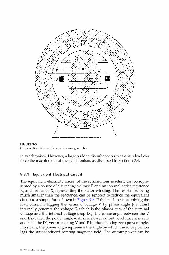
© 1999 by CRC Press LLC
in synchronism. However, a large sudden disturbance such as a step load canforce the machine out of the synchronism, as discussed in Section 9.3.4.
9.3.1 Equivalent Electrical Circuit
The equivalent electricity circuit of the synchronous machine can be repre-sented by a source of alternating voltage E and an internal series resistanceR
s
and reactance X
s
representing the stator winding. The resistance, beingmuch smaller than the reactance, can be ignored to reduce the equivalentcircuit to a simple form shown in Figure 9-6. If the machine is supplying theload current I lagging the terminal voltage V by phase angle
φ
, it mustinternally generate the voltage E, which is the phasor sum of the terminalvoltage and the internal voltage drop IX
s
. The phase angle between the Vand E is called the power angle
δ
. At zero power output, load current is zeroand so is the IX
s
vector, making V and E in phase having zero power angle.Physically, the power angle represents the angle by which the rotor positionlags the stator-induced rotating magnetic field. The output power can be
FIGURE 9-5
Cross section view of the synchronous generator.

© 1999 by CRC Press LLC
increased by increasing the power angle up to a certain limit, beyond whichthe rotor would no longer follow the stator field and will step out of thesynchronous mode of operation. In the nonsynchronous mode, it cannotproduce steady power.
9.3.2 Excitation Methods
The synchronous machine excitation system must be designed to producethe required magnetic field which is controllable to control the voltage andthe reactive power of the system. In modern high power machines, X
s
canbe around 1.5 units of the base impedance of the machine. With reactanceof this order, the phasor diagram of Figure 9-6 can show that the rotor filedexcitation required at rated load (100 percent load at 0.8 lagging powerfactor) is more than twice that at no load with the same terminal voltage.The excitation system has the corresponding current and voltage ratings,with capability of varying the voltage over a wide range of 1 to 3 or evenmore without undue saturation in the magnetic circuit. The excitation power,primarily to overcome the rotor winding I
2
R loss, ranges from to 1 percentof the generator rating. Most excitation systems operate at 200 to 1,000 Vdc.
For large machines, three types of excitation systems — DC, AC andstatic — are possible. In the DC system, a suitably designed DC generatorsupplies the main field winding excitation through conventional slip ringsand brushes. Due to low reliability and high maintenance requirement, theconventional DC machine is seldom used in the synchronous machine exci-tation system.
Most utility scale generators use the AC excitation system shown inFigure 9-7. The main exciter is excited by a pilot exciter. The AC output ofa permanent magnet pilot exciter is converted into DC by a floor standingrectifier and supplied to the main exciter through slip rings. The mainexciter’s AC output is converted into DC by means of phase controlledrectifiers, whose firing angle is changed in response to the terminal voltagevariations. After filtering the ripples, this direct current is fed to the synchro-nous generator field winding.
An alternative scheme is the static excitation, as opposed to the dynamicexcitation described in the preceding paragraph. In the static excitation
FIGURE 9-6
Equivalent electrical circuit and phasor diagram of synchronous machine.
12⁄

© 1999 by CRC Press LLC
scheme, the controlled DC voltage is obtained from a suitable stationary ACsource rectified and filtered. The DC voltage is then fed to the main fieldwinding through slip rings. This excitation scheme has a fast dynamicresponse and is more reliable because it has no rotating exciters.
The excitation control system modeling for analytical studies must be care-fully done as it forms a multiple feedback control system that can becomeunstable. The IEEE has developed industry standards for modeling the exci-tation systems. The model enters nonlinearly due to magnetic saturationpresent in all practical designs. The stability can be improved by supplement-ing the main control signal by auxiliary signals such as speed and power.
9.3.3 Electrical Power Output
The electrical power output of the synchronous machine is as follows:
(9-3)
Using the phasor diagram of Figure 9-6, the current can be expressed asfollows:
(9-4)
The real part of this current is
This part, when multiplied with the terminal voltage V gives the outputpower:
(9-5)
FIGURE 9-7
AC excitation system for synchronous generator.
P VI= cos φ
IE VjXs
E V ojXs
E j VjXs
= − = ∠ − ∠ =+( ) −δ δ δcos sin
IE
Xreal = ⋅ sin
s
δ.
PVEXs
= sinδ
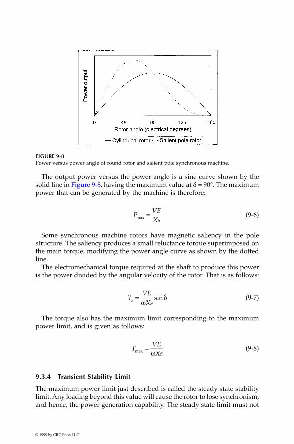
© 1999 by CRC Press LLC
The output power versus the power angle is a sine curve shown by thesolid line in Figure 9-8, having the maximum value at
δ
= 90°. The maximumpower that can be generated by the machine is therefore:
(9-6)
Some synchronous machine rotors have magnetic saliency in the polestructure. The saliency produces a small reluctance torque superimposed onthe main torque, modifying the power angle curve as shown by the dottedline.
The electromechanical torque required at the shaft to produce this poweris the power divided by the angular velocity of the rotor. That is as follows:
(9-7)
The torque also has the maximum limit corresponding to the maximumpower limit, and is given as follows:
(9-8)
9.3.4 Transient Stability Limit
The maximum power limit just described is called the steady state stabilitylimit. Any loading beyond this value will cause the rotor to lose synchronism,and hence, the power generation capability. The steady state limit must not
FIGURE 9-8
Power versus power angle of round rotor and salient pole synchronous machine.
PVEXsmax =
TVEXse =
ωδsin
TVEXsmax =
ω

© 1999 by CRC Press LLC
be exceeded under any condition, including those that can be encounteredduring transients. For example, if a sudden load step is applied to themachine initially operating in a steady state at load power angle
δ
1
(Figure 9-9), the rotor power angle would increase from
δ
1
to
δ
2
correspond-ing to the new load that it must supply. This takes some time depending onthe electromechanical inertia of the machine. No matter how short or longit takes, the rotor inertia and the electromagnetic restraining torque will setthe rotor in a mass-spring type of oscillatory mode, swinging the rotor powerangle beyond its new steady state value. If the power angle exceeds 90°during this swing, the machine stability and the power generation are lost.For this reason, the machine can be loaded only to the extent that even underthe worst-case step load, planned or accidental, or during all possible faults,the power angle swing will remain below 90° with sufficient margin. Thislimit on loading the machine is called the transient stability limit.
Equation 9-5 shows that the stability limit at given voltages can beincreased by designing the machine with low synchronous reactance X
s
,which is largely made of the stator armature reaction component.
9.4 Commercial Power Plants
The commercial power plants using the solar thermal system are beingexplored in a few hundred MWe capacity. Based on the Solar II power plantoperating experience, the design studies made by the National RenewableEnergy Laboratory for the U.S. Department of Energy have estimated the
FIGURE 9-9
Load step transient and stability limit of synchronous machine.

© 1999 by CRC Press LLC
performance parameters that are achievable for a 100 MWe commercialplant. Table 9-4 summarizes these estimates and compares with thoseachieved in the 10 MWe experimental Solar II power plant. The 100 MWeprototype design shows that the overall solar to electric efficiency of23 percent can be achieved in a commercial plant using the existing technol-ogy. For comparison, the conventional coal thermal plants typically operateat 40 percent conversion efficiency, and the photovoltaic power systems havethe overall solar-to-electricity conversion efficiency of 8 to 10 percent withamorphous silicon and 15 to 20 percent with crystalline silicon technologies.
Major conclusions of the studies to date are the following:
1. First plants as large as 100–200 MWe are possible to design andbuild based on the demonstrated technology to date. Future plantscould be larger.
2. The plant capacity factors up to 65 percent are possible, includingoutage.
3. Fifteen percent annual average solar-to-electric conversion effi-ciency is achievable.
4. The energy storage feature of the technology makes possible tomeet the peak demand on the utility lines.
5. Leveled energy cost is estimated to be 6 to 7 cents per kWh.6. A 100 MWe plant with a capacity factor of 40 percent requires 1.5
square miles of land.7. The capital cost of $2,000 per kWe capacity for first few commercial
plants and less for future plants.8. A comparable combined cycle gas turbine plant would cost
$1,000 kWe, which includes no fuel cost.9. Solar-fossil hybrids are the next step in development of this tech-
nology.
TABLE 9-4
Comparison of 10 MWe Solar II and 100 MWe Prototype Design
Performance ParameterSolar II Plant
10 MWeCommercial Plant
100 MWe
Mirror reflectivity 90% 94%Field efficiency 73% 73%Mirror cleanliness 95% 95%Receiver efficiency 87% 87%Storage efficiency 99% 99%Electromechanical conversion efficiency of generator 34% 43%Auxiliary components efficiency 90% 93%Overall solar-to-electric conversion efficiency 16% 23%
(Source: U.S. Department of Energy and Southern California Edison Company.)

© 1999 by CRC Press LLC
Compared to the pv and wind power, the solar thermal power technologyis less modular. Its economical size is estimated to be in the 100 to 300 MWerange. The cost studies at the National Renewable Energy Laboratory haveshown that a commercially designed utility-scale power plant using thecentral receiver power tower can produce electricity at a cost of 6 to 11 centsper kWh.
In other countries, the low temperature solar thermal power finds growingapplications. The high temperature applications, however, have yet todevelop on a large scale. An integrated combined cycle 40 MWe solar thermalwith 100 MWe gas turbine power plant is proposed at Jodhpur in Rajasthan,India. According to the Indian Renewable Energy Development Agency,India has the target to install 150 MWe solar thermal and photovoltaic capac-ity by the year 2002, and 1,500 MWe by 2012.
References
1. Mancini, T. 1994. “Solar thermal power today and tomorrow,”
Mechanical En-gineering, publication of the Institution of Mechanical Engineers,
London, August1994.
2. Southern California Edison Company. 1995.
Technology Report No. 14,
Irwindale,CA, Fall 1995.

© 1999 by CRC Press LLC
10
Energy Storage
Electricity is more versatile in use because it is a highly ordered form of energythat can be converted efficiently into other forms. For example, it can beconverted into mechanical form with efficiency near 100 percent or into heatwith 100 percent efficiency. The heat energy, on the other hand, cannot beconverted into electricity with high efficiency, because it is a disordered formof energy in atoms. For this reason, the overall thermal to electrical conversionefficiency of a typical fossil thermal power plant is under 40 percent.
A disadvantage of electricity is that it cannot be easily stored on a largescale. Almost all electrical energy used today is consumed as it is generated.This poses no hardship in conventional power plants, where the fuel con-sumption is varied with the load requirements. The photovoltaic and wind,being intermittent sources of power, cannot meet the load demand all of thetime, 24 hours a day, 365 days of the year. The energy storage, therefore, isa desired feature to incorporate with renewable power systems, particularlyin stand-alone plants. It can significantly improve the load availability, a keyrequirement for any power system.
The present and future energy storage technology that may be consideredfor stand-alone photovoltaic or wind power systems falls in the followingbroad categories:
• electrochemical battery.• flywheel.• compressed air.• superconducting coil.
10.1 Battery
The battery stores energy in the electrochemical form, and is the most widelyused device for energy storage in a variety of applications. The electrochem-ical energy is a semi-ordered form of energy, which is in between the electricaland thermal forms. It has one-way conversion efficiency of 85 to 90 percent.
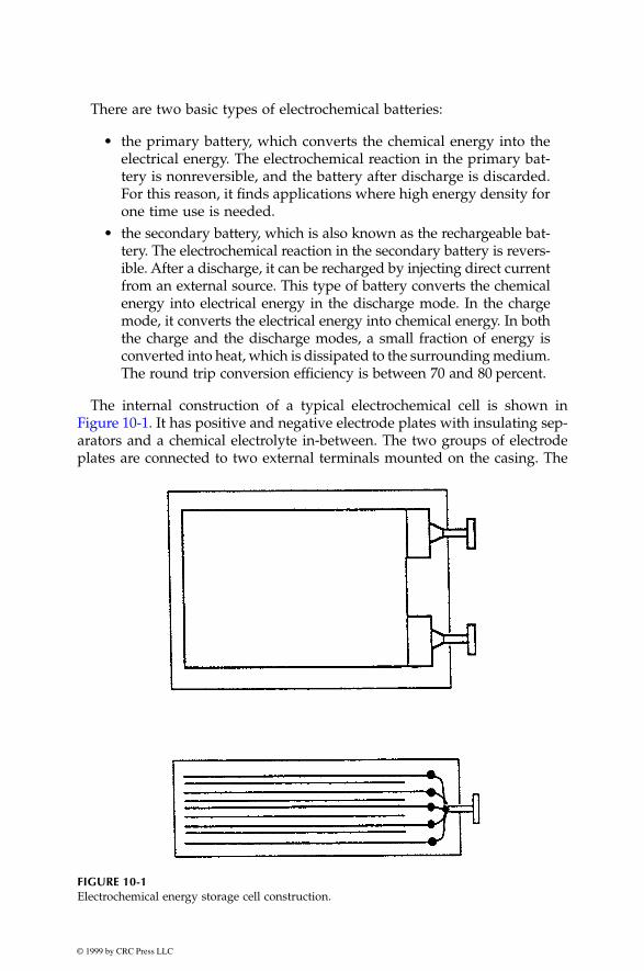
© 1999 by CRC Press LLC
There are two basic types of electrochemical batteries:
• the primary battery, which converts the chemical energy into theelectrical energy. The electrochemical reaction in the primary bat-tery is nonreversible, and the battery after discharge is discarded.For this reason, it finds applications where high energy density forone time use is needed.
• the secondary battery, which is also known as the rechargeable bat-tery. The electrochemical reaction in the secondary battery is revers-ible. After a discharge, it can be recharged by injecting direct currentfrom an external source. This type of battery converts the chemicalenergy into electrical energy in the discharge mode. In the chargemode, it converts the electrical energy into chemical energy. In boththe charge and the discharge modes, a small fraction of energy isconverted into heat, which is dissipated to the surrounding medium.The round trip conversion efficiency is between 70 and 80 percent.
The internal construction of a typical electrochemical cell is shown inFigure 10-1. It has positive and negative electrode plates with insulating sep-arators and a chemical electrolyte in-between. The two groups of electrodeplates are connected to two external terminals mounted on the casing. The
FIGURE 10-1
Electrochemical energy storage cell construction.

© 1999 by CRC Press LLC
cell stores electrochemical energy at low electrical potentials, typically a fewvolts. The cell capacity, denoted by C, is measured in Ampere-hours (Ah),meaning it can deliver C amperes for one hour or C/n amperes for n hours.
The battery is made of numerous electrochemical cells connected in aseries-parallel combination to obtain the desired operating voltage and cur-rent. The higher the battery voltage, the higher the number of cells requiredin series. The battery rating is stated in terms of the average voltage duringdischarge and the Ah capacity it can deliver before the voltage drops belowthe specified limit. The product of the voltage and the Ah forms the Whenergy rating it can deliver to a load from the fully-charged condition. Thebattery charge and discharge rates are stated in unit of its capacity in Ah.For example, charging a 100 Ah battery at C/10 rate means charging at 10A rate. Discharging that battery at C/2 rate means draining 50 A, at whichrate the battery will be fully discharged in 2 hours. The State of Charge (SOC)of the battery at any time is defined as the following:
10.2 Types of Batteries
There are at least six major rechargeable electrochemistries available today.They are as follows:
• lead-acid (Pb-acid).• nickel-cadmium (NiCd).• nickel-metal hydride (NiMH).• lithium-ion (Li-ion).• lithium-polymer (Li-poly).• zinc-air.
New electrochemistries are being developed by the United States AdvanceBattery Consortium for a variety of applications, such as electric vehicles,spacecraft, utility load leveling and, of course, for renewable power systems.
1
The average voltage during discharge depends on the electrochemistry, aslisted in Table 10-1. The energy density of various batteries, as measured byWh capacity per unit mass and per unit volume, are compared in Figure 10-2.The selection of the electrochemistry for a given application is a matter ofperformance and cost optimization.
Some construction and operating features of the above electrochemistriesare presented in the proceeding sections.
SOCAh= capacity remaining in the battery
Rated Ah capacity
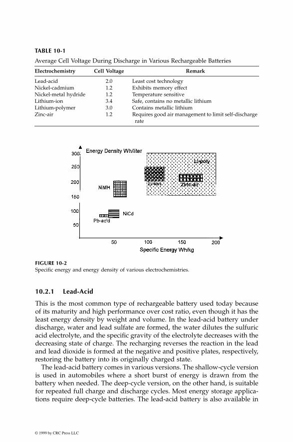
© 1999 by CRC Press LLC
10.2.1 Lead-Acid
This is the most common type of rechargeable battery used today becauseof its maturity and high performance over cost ratio, even though it has theleast energy density by weight and volume. In the lead-acid battery underdischarge, water and lead sulfate are formed, the water dilutes the sulfuricacid electrolyte, and the specific gravity of the electrolyte decreases with thedecreasing state of charge. The recharging reverses the reaction in the leadand lead dioxide is formed at the negative and positive plates, respectively,restoring the battery into its originally charged state.
The lead-acid battery comes in various versions. The shallow-cycle versionis used in automobiles where a short burst of energy is drawn from thebattery when needed. The deep-cycle version, on the other hand, is suitablefor repeated full charge and discharge cycles. Most energy storage applica-tions require deep-cycle batteries. The lead-acid battery is also available in
TABLE 10-1
Average Cell Voltage During Discharge in Various Rechargeable Batteries
Electrochemistry Cell Voltage Remark
Lead-acid 2.0 Least cost technologyNickel-cadmium 1.2 Exhibits memory effectNickel-metal hydride 1.2 Temperature sensitive Lithium-ion 3.4 Safe, contains no metallic lithiumLithium-polymer 3.0 Contains metallic lithiumZinc-air 1.2 Requires good air management to limit self-discharge
rate
FIGURE 10-2
Specific energy and energy density of various electrochemistries.

© 1999 by CRC Press LLC
sealed ‘gel-cell’ version with additives which turns the electrolyte into a non-spillable gel. Such batteries can be mounted sideways or upside down. Thehigh cost, however, limits its use in the military avionics.
10.2.2 Nickel Cadmium
The NiCd is a matured electrochemistry. The NiCd cell has positive elec-trodes made of cadmium and the negative electrodes of nickel hydroxide.Two electrodes are separated by Nylon
®
(registered trade name of E. I.Dupont Numerous and Company, Wilmington, Delaware) separators andpotassium hydroxide electrolyte in stainless steel casing. With sealed celland half the weight of conventional lead-acid, NiCd batteries have been usedto power most rechargeable consumer applications. They have a longer deepcycle life, and are more temperature tolerant than the lead-acid batteries.However, this electrochemistry has a memory effect (explained later), whichdegrades the capacity if not used for a long time. Moreover, cadmium hasrecently come under environmental regulatory scrutiny. For these reasons,the NiCd is being replaced by NiMH and Li-ion batteries in laptop computersand other similar high-priced consumer electronics.
10.2.3 Nickel-Metal Hydride
The NiMH is an extension of NiCd technology, and offers an improvementin energy density over that in NiCd. The major construction difference isthat the anode is made of a metal hydride. This eliminates the environmentalconcerns of cadmium. Another performance improvement is that it hasnegligible memory effect. The NiMH, however, is less capable of deliveringhigh peak power, has high self-discharge rate, and is susceptible to damagedue to overcharging. Compared to NiCd, NiMH is expensive at present,although the future price is expected to drop significantly. This expectationis based on current development programs targeted for large-scale applica-tion of this technology in electric vehicles.
10.2.4 Lithium-Ion
Lithium-ion technology is a new development, which offers three times theenergy density over that of lead-acid. Such large improvement in the energydensity comes from lithium’s low atomic weight of 6.9 versus 207 for lead.Moreover, the lithium-ion has higher cell voltage of 3.5 versus 2.0 for lead-acid and 1.2 for other electrochemistries. This requires fewer cells in seriesfor a given battery voltage, thus reducing the manufacturing cost.
On the negative side, the lithium electrode reacts with any liquid electro-lyte, creating a sort of passivation film. Every time when the cell is discharged

© 1999 by CRC Press LLC
and then charged, the lithium is stripped away, a free metal surface isexposed to the electrolyte and a new film is formed. To compensate, the celluses thick electrodes, adding into the cost. Or else, the life would be short-ened. For this reason, it is more expensive than NiCd.
In operation, the lithium-ion electrochemistry is vulnerable to damagefrom overcharging or other shortcomings in the battery management. There-fore, it requires more elaborate charging circuitry with adequate protectionagainst overcharging.
10.2.5 Lithium-Polymer
This is a lithium battery with solid polymer electrolytes. It is constructedwith a film of metallic lithium bonded to a thin layer of solid polymerelectrolyte. The solid polymer enhances the cell’s specific energy by actingas both the electrolyte and the separator. Moreover, the metal in solid elec-trolyte reacts less than it does with liquid electrolyte.
10.2.6 Zinc-Air
The zinc-air battery has a zinc negative electrode, a potassium hydroxideelectrolyte, and a carbon positive electrode, which is exposed to the air.During discharge, oxygen from the air is reduced at the carbon electrode(the so-called air cathode), and the zinc electrode is oxidized. During dis-charge, it absorbs oxygen from the air and converts into oxygen ions fortransport to the zinc anode. During charge, it evolves oxygen. A good airmanagement is essential for the performance of the zinc-air battery.
10.3 Equivalent Electrical Circuit
For steady-state electrical performance calculations, the battery is repre-sented by an equivalent circuit shown in Figure 10-3. In its simplest form,the battery works as a constant voltage source with small internal resistance.The open-circuit (or electrochemical) voltage E
i
of the battery decreaseslinearly with the Ah of discharge Q
d
, and the internal resistance R
i
increaseslinearly with Q
d
. That is, the battery open-circuit voltage is lower and theinternal resistance is higher in a partially discharged state as compared tothe E
o
and R
o
values in the fully charged state. Quantitatively,
(10-1)
where K
1
and K
2
are constants to be found by curve-fitting the test data.
E E K Q
R R K Q
i d
i d
= −
= +
0 1
0 2

© 1999 by CRC Press LLC
The terminal voltage drops with increasing load as shown by the V
b
linein Figure 10-4, and operating point is the intersection of the source line andthe load line (point P). The power delivered to the external load resistanceis I
2
R
L
.In fast discharge applications, such as for starting a heavily loaded motor,
the battery may be required to deliver the maximum possible power for ashort time. The peak power it can deliver can be derived using the maximumpower transfer theorem in electrical circuits. It states that the maximumpower can be transferred from the source to the load when the internalimpedance of the source equals the conjugate of the load impedance. Thebattery can deliver maximum power to a DC load when R
L
= R
i
. This givesthe following:
(10-2)
Since E
i
and R
i
vary with the state of charge, the P
max
also vary accordingly.The internal loss is I
2
R
i
. The efficiency at any state of charge is therefore:
FIGURE 10-3
Equivalent electrical circuit of the battery showing internal voltage and resistance.
FIGURE 10-4
Battery source line intersecting with load line at the operating point.
PERi
imax =
2
4

© 1999 by CRC Press LLC
(10-3)
The efficiency decreases as the battery is discharged, thus generating moreheat.
10.4 Performance Characteristics
The basic performance characteristics of the battery which influence thedesign are as follows:
• charge/discharge voltages.• charge/discharge ratio (c/d ratio).• round trip energy efficiency.• charge efficiency.• internal impedance.• temperature rise.• life in number of c/d cycles.
10.4.1 Charge/Discharge Voltages
The cell voltage variation during a typical charge/discharge cycle is shownin Figure 10-5 for cell with nominal voltage of 1.2 V, such as NiMH andNiCd. The voltage is maximum when the cell is fully charged (state of
FIGURE 10-5
Voltage variation during charge/discharge cycle of nickel-cadmium cell with nominal voltageof 1.2 volt.
η =+
RR R
L
L i

© 1999 by CRC Press LLC
charge = 1.0, or Ah discharged = 0). As the cell is discharged, the cell voltage(Vc) drops quickly to a plateau value of 1.2, which holds for a long time beforedropping to 1.0 at the end of its capacity (SOC = 0). In the reverse, when thecell is recharged, the voltage quickly rises to a plateau value of 1.45 and thenreaches a maximum value of 1.55 volts. The charge/discharge characteristicalso depends on how fast the battery is charged and discharged (Figure 10-6).
10.4.2 Charge/Discharge Ratio
After discharging certain Ah to load, the battery requires more Ah of chargeto restore the full state of charge. The charge/discharge ratio is defined asthe Ah input over the Ah output with no net change in the state of charge.This ratio depends on the charge and discharge rates and also on tempera-ture, as shown in Figure 10-7. At 20°C, for example, the charge/dischargeratio is 1.1, meaning the battery needs 10 percent more Ah than what wasdischarged for restoring to fully charged state.
10.4.3 Energy Efficiency
The energy efficiency over a round trip of full charge and discharge cycle isdefined as the ratio of the energy output over the energy input at the elec-trical terminals of the battery. For a typical battery of capacity C with anaverage discharge voltage of 1.2 V, average charge voltage of 1.45 V and thecharge/discharge ratio of 1.1, the efficiency is calculated as follows:
The energy output over the full discharge = 1.2
×
C
The energy input required to restore full charge = 1.45
×
1.1 C
FIGURE 10-6
Cell voltage curves at different charge/discharge rates.
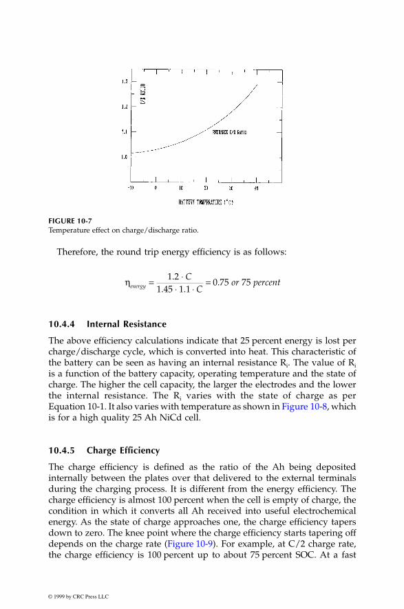
© 1999 by CRC Press LLC
Therefore, the round trip energy efficiency is as follows:
10.4.4 Internal Resistance
The above efficiency calculations indicate that 25 percent energy is lost percharge/discharge cycle, which is converted into heat. This characteristic ofthe battery can be seen as having an internal resistance R
i
. The value of R
i
is a function of the battery capacity, operating temperature and the state ofcharge. The higher the cell capacity, the larger the electrodes and the lowerthe internal resistance. The R
i
varies with the state of charge as perEquation 10-1. It also varies with temperature as shown in Figure 10-8, whichis for a high quality 25 Ah NiCd cell.
10.4.5 Charge Efficiency
The charge efficiency is defined as the ratio of the Ah being depositedinternally between the plates over that delivered to the external terminalsduring the charging process. It is different from the energy efficiency. Thecharge efficiency is almost 100 percent when the cell is empty of charge, thecondition in which it converts all Ah received into useful electrochemicalenergy. As the state of charge approaches one, the charge efficiency tapersdown to zero. The knee point where the charge efficiency starts tapering offdepends on the charge rate (Figure 10-9). For example, at C/2 charge rate,the charge efficiency is 100 percent up to about 75 percent SOC. At a fast
FIGURE 10-7
Temperature effect on charge/discharge ratio.
ηenergy
CC
= ⋅⋅ ⋅
=1 21 45 1 1
0 75 75.
. .. or percent

© 1999 by CRC Press LLC
charge rate of C/40, on the other hand, the charge efficiency at 60 percentSOC is only 50 percent.
10.4.6 Self-Discharge and Trickle Charge
Even with open-circuit terminals, the battery slowly self-discharges. In orderto maintain the full state of charge, it is continuously trickle-charged tocounter the self-discharge rate. This rate is usually less than one percent perday for most electrochemistries in normal working conditions.
After the battery is fully charged, the charge efficiency drops to zero. Anyadditional charge will be converted into heat. If overcharged at higher ratethan the self-discharge rate for an extended period, the battery would over-heat posing a safety hazard of potential explosion. For this reason, battery
FIGURE 10-8
Temperature effect on internal resistance in 25 Ah nickel-cadmium cell.
FIGURE 10-9
Charge efficiency versus state-of-charge at various charge rates.

© 1999 by CRC Press LLC
charge should have a regulator, which cuts back the charge rate to the trickle-rate once the battery is fully charged. Any excessive overcharging will pro-duce excessive gassing, which scrubs the electrode plates. Continuous scrub-bing at high rate produces excessive heat, and wears out electrodes leadingto shortened life. The trickle charging produces a controlled amount ofinternal gassing. It causes mixing action of the battery electrolyte, keepingit ready to deliver full charge.
10.4.7 Memory Effect
One major disadvantage of the NiCd battery is the memory effect. It is thetendency of the battery to remember the voltage at which it has deliveredmost of its capacity in the past. For example, if the NiCd battery is repeatedlycharged and discharged 25 percent of its capacity to point M in Figure 10-10,it will remember point M. Subsequently, if the battery is discharged beyondpoint M, the cell voltage will drop much below its original normal valueshown by the dotted line in Figure 10-10. The end result is the loss of fullcapacity after repeatedly using shallow discharge cycles. The phenomenonis like losing a muscle due to lack of use over a long time. A remedy forrestoring the full capacity is “reconditioning”, in which the battery is fullydischarged to almost zero voltage once every few months and then fullycharged to about 1.55 volts per cell. Other types of batteries do not have thememory effect.
10.4.8 Effects of Temperature
As seen in the preceding sections, the operating temperature significantlyinfluences the battery performance as follows:
FIGURE 10-10
Memory effect degrades discharge voltage in nickel-cadmium cell.

© 1999 by CRC Press LLC
• the capacity and the charge efficiency decrease with increasingtemperature. The capacity drops at temperatures above or belowcertain range, and drops sharply at temperatures below freezing.
• the self discharge rate increases with temperature.• the internal resistance increases as temperature decreases.
Table 10-2 shows the influence of temperature on the charge efficiency, thedischarge efficiency, and the self-discharge rate in the NiCd battery. Theprocess of determining the optimum operating temperature is also indicatedin the table. It is seen that different attributes have different desirable oper-ating temperature ranges. With all attributes jointly considered, the mostoptimum operating temperature is the intersection of all the desirable ranges.If we wish to limit the self discharge rate below 1 percent, and the chargeefficiency above 90 percent, Table 10-2 indicates that the optimum workingtemperature range is between –10°C and 25°C.
TABLE 10-2
Optimum Working Temperature Range for
Nickel-Cadmium Battery
Operating Temperature
°C
Charge Efficiency
Percent
Discharge Efficiency
PercentSelf-discharge Rate
% Capacity/Day
–40 0 72 0.1–35 0 80 0.1–30 15 85 0.1–25 40 90 0.2–20 75 95 0.2–15 85 97 0.2–10 90 100 0.2
–5 92 100 0.20 93 100 0.25 94 100 0.2
10 94 100 0.215 94 100 0.320 93 100 0.425 92 100 0.630 91 100 1.035 90 100 1.440 88 100 2.045 85 100 2.750 82 100 3.655 79 100 5.160 75 100 8.065 70 100 1270 60 100 20
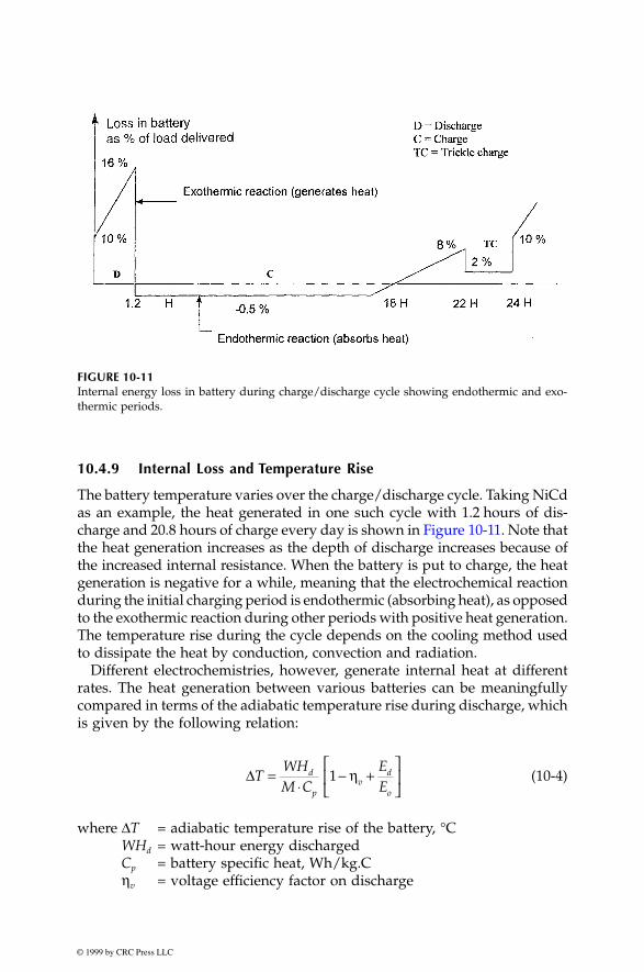
© 1999 by CRC Press LLC
10.4.9 Internal Loss and Temperature Rise
The battery temperature varies over the charge/discharge cycle. Taking NiCdas an example, the heat generated in one such cycle with 1.2 hours of dis-charge and 20.8 hours of charge every day is shown in Figure 10-11. Note thatthe heat generation increases as the depth of discharge increases because ofthe increased internal resistance. When the battery is put to charge, the heatgeneration is negative for a while, meaning that the electrochemical reactionduring the initial charging period is endothermic (absorbing heat), as opposedto the exothermic reaction during other periods with positive heat generation.The temperature rise during the cycle depends on the cooling method usedto dissipate the heat by conduction, convection and radiation.
Different electrochemistries, however, generate internal heat at differentrates. The heat generation between various batteries can be meaningfullycompared in terms of the adiabatic temperature rise during discharge, whichis given by the following relation:
(10-4)
where
∆
T
= adiabatic temperature rise of the battery, °C
WH
d
= watt-hour energy discharged
C
p
= battery specific heat, Wh/kg.C
η
v
= voltage efficiency factor on discharge
FIGURE 10-11
Internal energy loss in battery during charge/discharge cycle showing endothermic and exo-thermic periods.
∆TWHM C
EE
d
pv
d
o
=⋅
− +
1 η

© 1999 by CRC Press LLC
E
d
= average cell entropy energy per coulomb during discharge,i.e. average power loss per ampere of discharge, W/A
E
o
= average cell open circuit voltage, volts
For full discharge, the
WH
d
/
M
ratio in the above expression becomes thespecific energy. This indicates that higher specific energy cells would alsotend to have higher temperature rise during discharge, requiring enhancedcooling design. Various battery characteristics affecting the thermal designare listed in Table 10-3. Figure 10-12 depicts the adiabatic temperature rise
∆
T for various electrochemistries after a full discharge in short burst.
10.4.10 Random Failure
The battery fails when at least one cell fails. The cell failure is theoreticallydefined as the condition in which the cell voltage drops below certain low
TABLE 10-3
Battery Characteristics Affecting Thermal Design
Electrochemistry
Operating temperature
range °COvercharge
tolerance
Heat capacity Wh/kg-K
Mass density kg/liter
Entropic heating on discharge W/A-cell
Lead-acid –10 to 50 High 0.35 2.1 –0.06Nickel-cadmium –20 to 50 Medium 0.35 1.7 0.12Nickel-metal hydride –10 to 50 Low 0.35 2.3 0.07Lithium-ion 10 to 45 Very low 0.38 1.35 0Lithium-polymer 50 to 70 Very low 0.40 1.3 0
FIGURE 10-12
Adiabatic temperature rise for various electrochemistries.

© 1999 by CRC Press LLC
value before discharging rated capacity at room temperature. The low valueis generally taken as a 1.0 volt in cells with nominal voltage of 1.2 V. This isa very conservative definition of a battery failure. In practice, if one cellshows less than 1.0 V, other cells can make up without detecting the failureat the battery level. Even if all cells show stable voltage below 1.0 V at fullload, the load can be reduced to maintain the desired voltage for some timeuntil the voltage degrades further.
The cell can fail open, short, or somewhere in between (a soft short). Ashort that starts soft eventually develops into a hard short. In a low voltagebattery, any attempt to charge with a shorted cell may result in physicaldamage to the battery and/or the charge regulator. On the other hand, theshorted cell in a high voltage battery with numerous series connected cellsmay work forever. It, however, loses the voltage and Ah capacity, hence,would work as load on the healthy cells. An open cell, on the other hand,disables the entire battery of series-connected cells.
In a system having two parallel batteries, if one cell in one battery failsshort, the two batteries would have different terminal characteristics. Charg-ing or discharging such batteries as a group can result in highly unevencurrent sharing, subsequently overheating one of the batteries. Two remediesare available to avoid this. One is to charge and discharge both batterieswith individual current controls such that they both draw their rated shareof the load. The other is to replace the failed cell immediately, which cansometimes be impractical. In general, the individual charge/discharge con-trol for each battery is the best strategy. It may also allow replacement ofany one battery with different electrochemistry or different age, which wouldhave different load sharing characteristics. Batteries are usually replacedseveral times during the economic life of the plant.
10.4.11 Wear-Out Failure
In addition to the random failure, the battery has the wear out failure mode.It is associated with the electrode wear due to repeated charge/dischargecycles. The number of times the battery can be discharged and rechargedbefore the electrodes wear out depends on the electrochemistry. The batterylife is measured in the number of charge/discharge cycles it can deliverbefore failure. The life depends strongly on the depth of discharge and thetemperature as shown in Figure 10-13 for high quality NiCd batteries. Thelife also depends, to a lesser degree, on the electrolyte concentration and theelectrode porosity and thickness. The former factors are application related,whereas the latter are construction related.
It is noteworthy from Figure 10-14 that the life at a given temperature isan inverse function of the depth of discharge. If the life is 100 units at50 percent DoD, then it would be 200 units at 25 percent DoD. This makesthe product of the cycles to fail and the DoD remain constant. This productdecreases with increasing temperature. Such is true for most batteries. This

© 1999 by CRC Press LLC
means that the battery at a given temperature can deliver the same numberof equivalent full cycles of energy regardless of the depth of discharge. Thetotal Wh energy the battery can deliver over its life is approximately constant.Such observation is useful in comparing the costs of various batteries for agiven application.
The life consideration is the dominant design driver in the battery sizing.Even when the load may be met with a smaller capacity, the battery isoversized to meet the life requirement as measured in number of charge/dis-charge cycles. For example, with the same Wh load, the battery that mustcharge/discharge twice as many cycles per period needs approximatelydouble the capacity to have the same calendar life.
FIGURE 10-13
Charge/discharge cycle life of sealed nickel-cadmium battery versus temperature and depthof discharge.
FIGURE 10-14
Lead-acid battery capacity variations with temperature.

© 1999 by CRC Press LLC
10.4.12 Various Batteries Compared
The performance characteristics and properties of various electrochemistriespresented in the preceding sections are summarized and compared inTables 10-4 and 10-5. Note that the overall cost of the lead-acid battery islow compared to NiCd, NiMH and Li-ion batteries. Because of its least costper Wh delivered over the life, the lead-acid battery has been the workhorseof the industry.
2
10.5 More on Lead-Acid Battery
The lead-acid battery is available in small to large capacities in variousterminal voltages, such as 6 V, 12 V and 24 V. Like in other batteries, the Ahcapacity of the lead-acid battery is sensitive to temperature. Figure 10-14shows the capacity variations with temperature for deep-cycle lead-acidbatteries. At –20°F, for example, the high-rate battery capacity is about20 percent of its capacity at 100°F. The car is hard to start in winter for thisreason. On the other hand, the self-discharge rate decreases significantly atcold temperatures, as seen in Figure 10-15.
TABLE 10-4
Specific Energy and Energy Density of Various Batteries
ElectrochemistrySpecific Energy
Wh/kgEnergy Density
Wh/liter
SpecificPowerW/kg
PowerDensityW/liter
Lead-acid 30–40 70–75 ~200 ~400Nickel-cadmium 40–60 70–100 150–200 220–350Nickel-metal hydride 50–65 140–200 ~150 450–500Lithium-ion 90–120 200–250 200–220 400–500Lithium-polymer 100–200 150–300 >200 >350Zinc-air 140–180 200–220 ~150 ~200
TABLE 10-5
Life and Cost Comparison of Various Batteries
ElectrochemistryCycle life in full discharge cycles
Calendar life in years
Self discharge rate%/month at
25 °C
Relative cost
$/kWh
Lead-acid 500–1000 5–8 3–5 200–500Nickel-cadmium 1000–2000 10–15 20–30 1500Nickel-metal hydride 1000–2000 8–10 20–30 2500Lithium-ion 500–1000 — 5–10 3000Lithium-polymer 500–1000 — 1-2 >3000Zinc-air 200–300 — 4–6 —
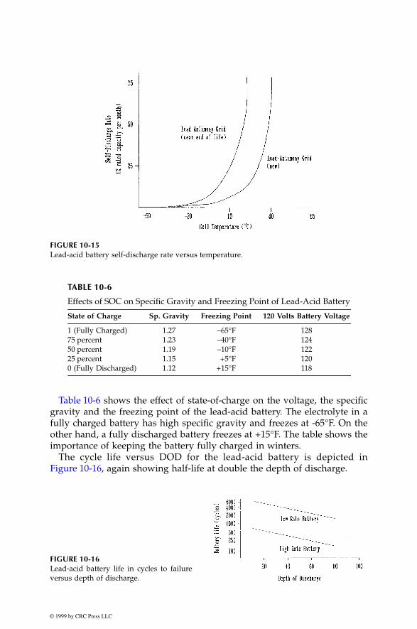
© 1999 by CRC Press LLC
Table 10-6 shows the effect of state-of-charge on the voltage, the specificgravity and the freezing point of the lead-acid battery. The electrolyte in afully charged battery has high specific gravity and freezes at -65°F. On theother hand, a fully discharged battery freezes at +15°F. The table shows theimportance of keeping the battery fully charged in winters.
The cycle life versus DOD for the lead-acid battery is depicted inFigure 10-16, again showing half-life at double the depth of discharge.
FIGURE 10-15
Lead-acid battery self-discharge rate versus temperature.
TABLE 10-6
Effects of SOC on Specific Gravity and Freezing Point of Lead-Acid Battery
State of Charge Sp. Gravity Freezing Point 120 Volts Battery Voltage
1 (Fully Charged) 1.27 –65°F 12875 percent 1.23 –40°F 12450 percent 1.19 –10°F 12225 percent 1.15 +5°F 1200 (Fully Discharged) 1.12 +15°F 118
FIGURE 10-16
Lead-acid battery life in cycles to failureversus depth of discharge.

© 1999 by CRC Press LLC
The discharge rate influences the lead-acid battery capacity, as shown inFigure 10-17. The shorter the discharge time (i.e., higher the discharge rate),the lower the Ah capacity the battery can deliver.
The lead-acid cell voltage is 2.0 volts nominal, and the internal resistanceis around one milliohm per cell. The cycle life is 500-1,000 full charge dis-charge cycles for medium rate batteries. The operating temperature range isbetween –20 to 50°C and the survival temperature is –55 to 60°C.
10.6 Battery Design
The battery design for given application depends on the following systemrequirements:
• voltage and current.• charge and discharge rates and duration.• operating temperature during charge and discharge.• life in number of charge and discharge cycles.• cost, size, and weight constraints.
Once these system level design parameters are identified, the batterydesign proceeds in the following steps:
• select the electrochemistry suitable for the overall system require-ments.
• determine the number of series cells required to meet the voltagerequirement.
• determine the Ah discharge required to meet the load demand.
FIGURE 10-17
Lead-acid battery capacity with discharge time.

© 1999 by CRC Press LLC
• for the required number of charge/discharge cycles, determine themaximum allowable depth of discharge.
• the total Ah capacity of the battery is then determined by dividingthe Ah discharge required by the allowable depth of dischargecalculated above.
• determine the number of battery packs required in parallel for thetotal Ah capacity.
• determine the temperature rise and the thermal controls required.• provide the charge and discharge rate controls as needed.
Each cell in the battery pack is electrically insulated from each other andfrom the ground. The electrical insulation must be good conductor of heatto maintain low temperature gradient between the cells and also to theground.
The battery performs better under slow charge and discharge rates. Itaccepts less energy when charged at a faster rate. Also the faster the dischargerate, the faster the voltage degradation and lower the available capacity tothe load. For these reasons, high charge and discharge rate applicationsrequire different design considerations than the low rate applications.
10.7 Battery Charging
During the battery charging, the energy management software monitors thestate-of-charge, the overall health, and the safe termination criteria. Theoperating parameters monitored are the voltage, the current, and the tem-perature. The charging timer is started after all initial checks are successfullycompleted. Charging may be suspended (but not reset) if it detects violationof critical safety criteria. The timer stops charging if the defect persistsbeyond a certain time limit.
The normal charging has the following three phases:
• bulk (fast) charge, which deposits 80 to 90 percent of the drainedcapacity.
• taper charge in which the charge rate is gradually cut back to topoff the remaining capacity.
• trickle (float) charge after the battery is fully charged to counter theself-discharge rate.
The bulk charge and the taper charge termination criteria are preloaded inthe battery management software to match with the battery electrochemistryand the system design parameters. For example, the NiCd and NiMH bat-teries are generally charged at constant current (Figure 10-18), terminating
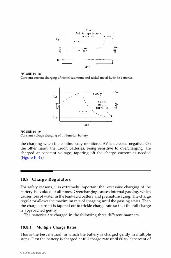
© 1999 by CRC Press LLC
the charging when the continuously monitored
∆
V is detected negative. Onthe other hand, the Li-ion batteries, being sensitive to overcharging, arecharged at constant voltage, tapering off the charge current as needed(Figure 10-19).
10.8 Charge Regulators
For safety reasons, it is extremely important that excessive charging of thebattery is avoided at all times. Overcharging causes internal gassing, whichcauses loss of water in the lead-acid battery and premature aging. The chargeregulator allows the maximum rate of charging until the gassing starts. Thenthe charge current is tapered off to trickle charge rate so that the full chargeis approached gently.
The batteries are charged in the following three different manners.
10.8.1 Multiple Charge Rates
This is the best method, in which the battery is charged gently in multiplesteps. First the battery is charged at full charge rate until 80 to 90 percent of
FIGURE 10-18
Constant current charging of nickel-cadmium and nickel-metal-hydride batteries.
FIGURE 10-19
Constant voltage charging of lithium-ion battery.

© 1999 by CRC Press LLC
the capacity is achieved. The charge current is then cut back, in steps, untilthe battery is fully charged. At this time, the charge current is further reducedto trickle-charge rate, keeping it fully charged until the next load demandcomes on the battery. This method, therefore, needs at least three chargerates in the charge regulator design.
10.8.2 Single Charge Rate
This method uses a simple low cost regulator which is either on or off. Theregulator is designed for only one charge rate. When the battery is fullycharged, as measured by its terminal voltage, the charger is turned off by arelay. When the battery voltage drops below a preset value, the charger isagain connected in full force. Since the charging is not gentle in this method,full charge is difficult to achieve and maintain. An alternate version of thischarging method is the multiple pulse charging. Full current charges thebattery up to the high preset voltage just below the gassing threshold. Atthis time, the charger is shut off for a short time to allow the battery chemicalsto mix and voltage to fall. When the voltage falls below the low presetthreshold, the charger is reconnected, again passing full current to the battery.
10.8.3 Unregulated Charging
This least cost method can be used in photovoltaic power systems. It usesno charge regulator. The battery is charged directly from a solar modulededicated just for charging. The charging module is properly designed forsafe operation for the given number of cells in the battery. For example, in12 volts lead-acid battery, the maximum photovoltaic module voltage is keptbelow 15 V, thus, making it difficult to overcharge. When the battery is fullycharged, the array is fully shunted to ground by a shorting switch (transis-tor). The shunt transistor switch is open when the battery voltage dropsbelow certain value. The isolation diode blocks the battery powering thearray or the shunt at night, a discussed in Section 8.8.
10.9 Battery Management
Drawing the electrical power from the battery when needed, and chargingit back when access power is available, requires a well-controlled charge anddischarge process. Otherwise, the battery performance could suffer, the lifeshortened and the maintenance increased. Some common performance prob-lems are as follows:
• low charge efficiency resulting in low state of charge.• loss of capacity to hold the rated Ah charge.
© 1999 by CRC Press LLC
• excessive gassing and heating, leading to a short life.• unpredictable premature failure leading to loss of load availability.• positive plate corrosion shortening the life.• stratification and sulfation degrading the performance.
The following features incorporated in the battery management can avoidthe above problems:
• controlled voltage charging, preferably at constant voltage.• temperature-compensated charging, in that the charge termination
occurs earlier if the battery temperature is higher than the referencetemperature.
• individual charge control if two or more batteries are charged inparallel.
• accurate set points to start and to stop the charge and dischargemodes.
10.9.1 Monitoring and Controls
The batteries in modern power systems are managed by dedicated computersoftware. The software monitors and controls the following performanceparameters:
• voltage and current.• temperature and pressure (if applicable).• ampere-hour in and out of the battery.• state of charge and discharge.• rate of charge and discharge.• depth of discharge.• number of charge and discharge cycles
The Ah integrating meter is commercially available, which keeps track of theAh in and out of the battery and sends required signals to the mode controller.
The temperature compensation on the maximum battery voltage and thestate-of-charge can improve the battery management, particularly in extremecold temperatures. It can allow additional charging during cold periodswhen the battery can accept more charge. The low voltage alarm is a goodfeature to have, as excessive discharging below the threshold low voltagecan cause cell voltage reversal, leading to battery failure. The alarm can beused to shed noncritical loads from the battery to avoid battery damage.
Figure 10-20 depicts a commercially available battery management systemincorporating a dedicated microprocessor with software.
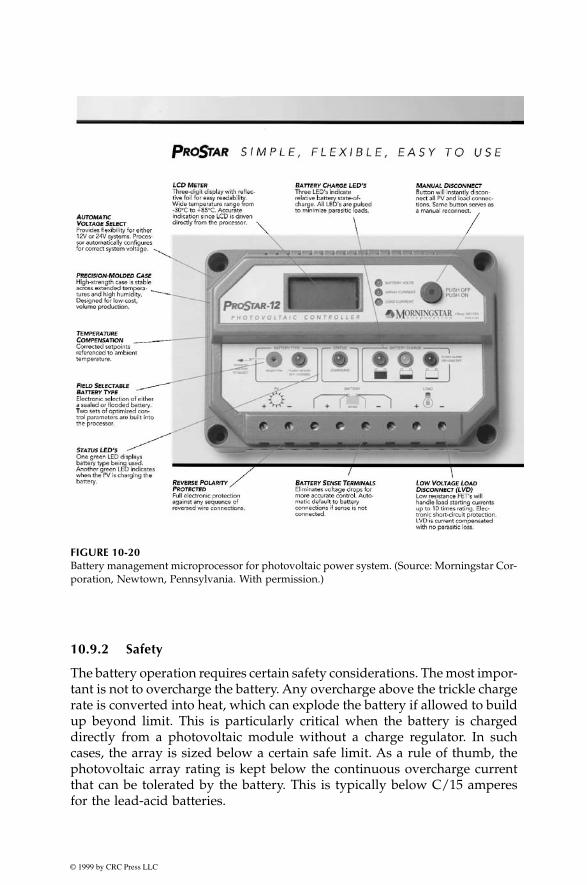
© 1999 by CRC Press LLC
10.9.2 Safety
The battery operation requires certain safety considerations. The most impor-tant is not to overcharge the battery. Any overcharge above the trickle chargerate is converted into heat, which can explode the battery if allowed to buildup beyond limit. This is particularly critical when the battery is chargeddirectly from a photovoltaic module without a charge regulator. In suchcases, the array is sized below a certain safe limit. As a rule of thumb, thephotovoltaic array rating is kept below the continuous overcharge currentthat can be tolerated by the battery. This is typically below C/15 amperesfor the lead-acid batteries.
FIGURE 10-20
Battery management microprocessor for photovoltaic power system. (Source: Morningstar Cor-poration, Newtown, Pennsylvania. With permission.)

© 1999 by CRC Press LLC
10.10 Flywheel
The flywheel stores kinetic energy in a rotating inertia. This energy can beconverted from and to electricity with high efficiency. The flywheel energystorage is an old concept, which is getting commercially viable due toadvances made in high strength, light-weight fiber composite rotors, and themagnetic bearings that operates at high speeds. The flywheel energy storagesystem is being developed for a variety of applications, and is expected tomake significant inroads in the near future. The round trip conversion effi-ciency of a large flywheel system can approach 90 percent, much higher thanthat in the battery.
The energy storage in the flywheel is limited by the mechanical stress dueto centrifugal force at high speed. Small to medium-size flywheels have beenin use for years. Considerable development efforts are underway around theworld for high-speed flywheels to store large amounts of energy. The presentgoal of these developments is to achieve five times the energy density of thecurrently available secondary batteries. This goal is achievable with thefollowing enabling technologies, which are already in place in their compo-nent forms:
• high-strength fibers having ultimate tensile strength of over onemillion psi.
• advances made in designing and manufacturing fiber-epoxy com-posites.
• high-speed, magnetic bearings which eliminate friction, vibrations,and noise.
The flywheel system is made of a composite fiber rotor supported onmagnetic bearings rotating in a vacuum, and coupled with a brushless motor-generator machine. Two counter-rotating wheels are placed side by side inmoving vehicles where gyroscopic effects must be eliminated.
10.10.1 Energy Relations
The energy stored in flywheel having the moment of inertia J rotating at theangular speed
ω
is given by the following:
(10-5)
The centrifugal force in the rotor material of density
ρ
at radius r is givenby
ρ
(r
ω
)
2
, which is supported by the hoop stress in the rotor rim. Since thelinear velocity V = 2
π
r
ω
, the maximum centrifugal stress in the rotor is
E J= ⋅12
2ω

© 1999 by CRC Press LLC
proportional to the square of the outer tip velocity. The allowable stress inthe material places an upper limit on the rotor tip speed. Therefore, smallerrotors can run at high speed, and vice versa. The thin rim type rotors havehigh inertia, and, hence, stores more energy per unit of weight. For thisreason, most energy storage rotors have annular rim type construction. Forsuch rotor with inner radius R1 and the outer radius R2, it can be shown thatthe maximum energy that can be stored for an allowable rotor tip velocityV is as follows:
(10-6)
where K1 is the proportionality constant. The thin rim flywheel with R1/R2 →1 results in high specific energy for given allowable stress. The higher theultimate strength of the material, the higher is the specific energy. The lowerthe material density, the lower the centrifugal stress produced, and, therefore,higher the allowable speed and the specific energy. The Emax can thereforebe expressed as follows:
(10-7)
where K2 is another proportionality constant, σmax is the maximum allowablehoop stress and ρ is the mass density of the rotor material. A good flywheeldesign therefore has high σmax /ρ ratio for high specific energy. It also hashigh E/ρ ratio for rigidity, where E is the Young’s modulus of elasticity.
The metallic flywheel has low specific energy because of low σmax /ρ ratio,whereas the high strength polymer fiber, such as graphite, silica and boron,having much higher σmax /ρ ratio, store an order of magnitude higher energyper unit of weight. Table 10-7 compares the specific energy of various metal-lic and polymer fiber composite rotors. In addition to the high specific energy,the composite rotor has a safe mode of failure, as it disintegrates to fluffrather than fragmenting like the metal flywheel.
Figure 10-21 shows a rotor design recently developed at the OakridgeNational Laboratory. The fiber/epoxy composite rim is made of two rings.The outer ring is made of high-strength graphite, and the inner ring of low-cost glass fibers. The hub is made of single piece aluminum in the radialspoke form. Such construction is cost effective because it uses costly materialonly where it is needed for strength. That is in the outer ring where thecentrifugal stress is the maximum, resulting in high hoop stress.
Figure 10-22 shows a prototype 5 kWh flywheel weight and specific energy(Wh per unit weight) versus σmax /ρ ratio of the material. It is noteworthythat the weight decreases inversely and the specific energy increases linearlywith σmax /ρ.
E K VRRmax = ⋅ ⋅ +
1
2 1
2
2
1
E Kmaxmax= 2
σρ

© 1999 by CRC Press LLC
10.10.2 Flywheel System Components
The complete flywheel energy storage system requires the following com-ponents:
• high-speed rotor attached to the shaft via strong hub.• bearings with good lubrication system or with magnetic suspension.• electromechanical energy converter, usually one machine which
can work as a motor during charging, and as a generator whiledischarging the energy.
• power electronics to drive the motor and to condition the generatorpower.
• control electronics for controlling the magnetic bearings and otherfunctions.
TABLE 10-7
Maximum Specific Energy Storable in a Thin Rim Flywheel with Various Rim Materials
Wheel MaterialMaximum Specific Energy
Storable Wh/kg
Aluminum alloy 25Maraging steel 50E-glass composite 200Carbon fiber composite 220S-glass composite 250Polymer fiber composite 350Fused silica fiber composite 1000Lead-acid battery 30–40Lithium-ion battery 90–120
FIGURE 10-21Flywheel rotor design using two composite rings. (Adapted from the DOE/Oakridge NationalLaboratory’s prototype design.)

© 1999 by CRC Press LLC
Good bearings have low friction and vibration. Conventional bearings areused up to speeds in a few tens of thousands rpm. Speeds approaching100,000 rpm are possible by using magnetic bearings, which support therotor by magnetic repulsion and attraction. The mechanical contact is elim-inated, thus eliminating the friction. The windage is eliminated by runningthe rotor in vacuum.
Magnetic bearings come in a variety of configurations using permanentmagnets and dynamic current actuators to achieve the required restraints. Arigid body can have six degrees of freedom. The bearings retain the rotor infive degrees of freedom, leaving one for rotation. The homopolar configurationis depicted in Figure 10-23. The permanent magnets are used to provide freelevitation support of the shaft. The permanent magnet bias also helps stabilizethe shaft under a rotor drop. The electromagnet coils are used for stabilizationand control. The control coils operate at low duty cycle, and only one servocontroller loop is needed for each axis. The servo control coils provide activecontrol to maintain the shaft stability by providing restoring forces as neededto maintain the shaft in the centered position. The position and velocity sensorsare used in the active feedback loop. The electric current variation in theactuator coils compels the shaft to remain centered in the air gaps.
Small flux pulsation as the rotor rotates around the discrete actuator coilsproduce small electromagnetic loss in the metallic parts. This loss, however,is negligible compared to the loss due to friction in conventional bearings.
In the flywheel system configuration, the rotor can be located radiallyoutward, as shown in Figure 10-24. It forms a volume-efficient packaging.The magnetic bearing has permanent magnets inside. The magnetic fluxtravels through the pole shoes on the stator and the magnetic feedback ringon the rotor. The reluctance lock between the pole shoes and the magneticfeedback ring provides the vertical restraint. The horizontal restraint is pro-vided by two sets of the dynamic actuator coils. The currents in the coils arecontrolled in response to the feedback loop controlling the rotor position.
FIGURE 10-22Specific energy versus specific strength in flywheel design.

© 1999 by CRC Press LLC
The electromechanical energy conversion is achieved with one machine,which works as a motor for spinning up the rotor for energy charge, and asa generator while decelerating the rotor for discharge. Again, two types of
FIGURE 10-23Avcon’s patented homopolar permanent magnet active bearing. (Source: Avcon Inc., WoodlandHills, California. With permission.)
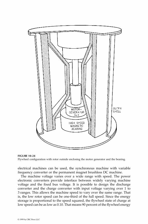
© 1999 by CRC Press LLC
electrical machines can be used, the synchronous machine with variablefrequency converter or the permanent magnet brushless DC machine.
The machine voltage varies over a wide range with speed. The powerelectronic converters provide interface between widely varying machinevoltage and the fixed bus voltage. It is possible to design the dischargeconverter and the charge converter with input voltage varying over 1 to3 ranges. This allows the machine speed to vary over the same range. Thatis, the low rotor speed can be one-third of the full speed. Since the energystorage is proportional to the speed squared, the flywheel state of charge atlow speed can be as low as 0.10. That means 90 percent of the flywheel energy
FIGURE 10-24Flywheel configuration with rotor outside enclosing the motor generator and the bearing.

© 1999 by CRC Press LLC
can be discharged with no hardship on the power electronics, or othercomponents of the system.
As to the number of charge-discharge cycles the flywheel can withstand,the fatigue life of the composite rotor is the limiting factor. Experience indi-cates that the polymer fiber composites in general have a longer fatigue lifethan solid metals. The properly-designed flywheel, therefore, can last muchlonger than the battery and can discharge to a much deeper level. Flywheelsmade of composite rotors have been fabricated and tested to demonstratemore than 10,000 cycles full charge and discharge. This is an order of mag-nitude more than any battery presently available.
10.10.3 Flywheel Benefits Over Battery
The main advantages of the flywheel energy storage over the battery are asfollows:
• high energy storage capacity per unit of weight and volume.• high depth of discharge.• long cycle life, which is insensitive to the depth of discharge.• high peak power capability without overheating concerns.• easy power management, as the state of charge is simply measured
by the speed.• high round trip energy efficiency.• flexibility in designing for a given voltage and current.• improved quality of power as the electrical machine is stiffer than
the battery.
These benefits have the potential of making the flywheel the least-costenergy storage alternative per Wh delivered over the operating life.
10.11 Compressed Air
The compressed air energy storage system consists of:
• air compressor.• expansion turbine.• electric motor-generator.• overhead storage tank or an underground cavern.
The energy stored in compressed air is given by the following derivations.

© 1999 by CRC Press LLC
If P and V represent the air pressure and volume, respectively, and if theair compression from pressure P1 to P2 follows the gas law PVn = constant,then the work required during this compression is the energy stored in thecompression air. It is given by the following:
(10-8)
And the temperature at the end of the compression is given by the following:
(10-9)
When the elevated temperature air at the end of the constant volumecompression cools down, a part of the pressure is lost with the correspondingdecrease in the stored energy.
The smaller the value of n, the smaller the energy stored. The isentropicvalue of n for air is 1.4. Under normal working conditions, n is about 1.3.
The electrical power is generated by venting the compressed air throughan expansion turbine which drives the generator. The compressed air systemmay work under constant-volume or constant-pressure.
In the constant-volume compression, the compressed air is stored in pres-sure tanks, mine caverns, depleted oil or gas fields, or abandoned mines.One million cubic feet of air storage at 600 psi provide an energy storagecapacity enough to supply about million kWhe. This system, however, hasa disadvantage. The air pressure reduces as the compressed air is depletedfrom the storage, and the electrical power output decreases with the decreas-ing pressure.
In the constant-pressure compression, the air storage may be in an aboveground variable-volume tank or an underground aquifer. One million cubicfeet of air storage at 600 psi provide an energy storage capacity enough tosupply about 0.07 million kWhe. A variable-volume tank maintains a con-stant pressure by the weight on the tank cover. If aquifer is used, the pressureremains approximately constant while the storage volume increases becauseof water displacement in the surrounding rock formation. During electricgeneration, the water displacement of the compressed air causes a decreaseof only a few percentages in the storage pressure, keeping the electricalgeneration rate essentially constant.
The energy storage efficiency of the compressed air-storage system is afunction of a series of component efficiencies, such as the compressor efficiency,the motor-generator efficiency, heat losses, and the compressed air leakage.The overall round trip efficiency of about 50 percent has been estimated.
Energy stored =−( )
−n P V PV
n2 2 1 1
1
TT
PP
nn
2
1
2
1
1
=
−
14⁄

© 1999 by CRC Press LLC
10.12 Superconducting Coil
The development efforts to use the superconducting technology for storingelectrical energy has started yielding highly promising results. In its workingprinciple, the energy is stored in the magnetic field of a coil, and is given bythe following expression:
(10-10)
where B = the magnetic field density produced by the coil, Teslaµ = magnetic permeability of air = 4 π 10–7 henry/meterL = inductance of the coil, henry
The coil must carry current in order to produce the required magneticfield. The current requires a voltage to be applied to the coil terminals. Therelation between the coil current I and the voltage V is as follows:
(10-11)
where R and L are the resistance and inductance of the coil, respectively. Forstoring energy in a steady state, the second term in Equation 10-11 must bezero. Then the voltage required to circulate the needed current is simply V =R · I.
The resistance of the coil is temperature dependent. For most conductingmaterials, it is higher at higher temperature. If the temperature of the coil isreduced, the resistance drops as shown in Figure 10-25. In certain materials,the resistance abruptly drops to a precise zero at some critical temperature.In the figure, this point is shown as Tc. Below this temperature, no voltageis required to circulate current in the coil, and the coil terminals can beshorted. The current will continue to flow in the coil indefinitely, with thecorresponding energy stored in the coil also indefinitely. The coil is said tohave attained the superconducting state, one which has attained preciselyzero resistance. The energy in the coil then freezes.
Although the superconducting phenomenon was discovered decades ago,industry interest in developing practical applications started in the early 1970s.In the U.S.A., the pioneering work has been done in this field by the GeneralElectric Company, the Westinghouse Research Center and the University ofWisconsin. During the 1980s, a grid-connected 8 kWh superconducting energystorage system was built with funding from the Department of Energy, andwas operated by the Bonneville Power Administration in Portland, Oregon.
Energy stored in a coil B Joules m
I L Joules
2 3
2
= µ
= ⋅
12
12
V RI Ldidt
= +
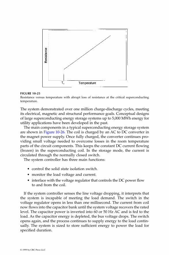
© 1999 by CRC Press LLC
The system demonstrated over one million charge-discharge cycles, meetingits electrical, magnetic and structural performance goals. Conceptual designsof large superconducting energy storage systems up to 5,000 MWh energy forutility applications have been developed in the past.
The main components in a typical superconducting energy storage systemare shown in Figure 10-26. The coil is charged by an AC to DC converter inthe magnet power supply. Once fully charged, the converter continues pro-viding small voltage needed to overcome losses in the room temperatureparts of the circuit components. This keeps the constant DC current flowing(frozen) in the superconducting coil. In the storage mode, the current iscirculated through the normally closed switch.
The system controller has three main functions:
• control the solid state isolation switch.• monitor the load voltage and current.• interface with the voltage regulator that controls the DC power flow
to and from the coil.
If the system controller senses the line voltage dropping, it interprets thatthe system is incapable of meeting the load demand. The switch in thevoltage regulator opens in less than one millisecond. The current from coilnow flows into the capacitor bank until the system voltage recovers the ratedlevel. The capacitor power is inverted into 60 or 50 Hz AC and is fed to theload. As the capacitor energy is depleted, the bus voltage drops. The switchopens again, and the process continues to supply energy to the load contin-ually. The system is sized to store sufficient energy to power the load forspecified duration.
FIGURE 10-25Resistance versus temperature with abrupt loss of resistance at the critical superconductingtemperature.

© 1999 by CRC Press LLC
The superconducting energy storage has several advantages over othertechnologies:
• the round trip efficiency of the charge-discharge cycle is high at95 percent. This is higher than that attainable by any other tech-nology.
• much longer life, up to about 30 years.• the charge and discharge times can be extremely short, making it
attractive for supplying large power for a short time if needed.• has no moving parts in the main system, except in the refrigeration
components.
In the superconducting energy storage system, the main cost is to keepthe coil below the critical superconducting temperature. Until now the nio-bium-titanium alloy has been extensively used, which has the critical tem-perature of about 9°K. This requires liquid helium as coolant at around 4°K.The 1986 discovery of high temperature superconductors has accelerated theindustry interest in this technology. Three types of high temperature super-conducting materials are available now, all made from bismuth or yttrium-cuprate compounds. These superconductors have the critical temperaturearound 100°K. Therefore, they can be cooled by liquid nitrogen, which needsorders of magnitude less refrigeration power. As a result, numerous pro-
FIGURE 10-26Superconducting energy storage schematic.

© 1999 by CRC Press LLC
grams around the world have started to develop commercial applications.Toshiba Corporation of Japan and GEC-Alsthom along with Electricite deFrance are actively perusing development in this field.3-4
References
1. Riezenman, M. J. 1995. “In search of better batteries,” IEEE Spectrum, p. 51-56,May 1995.
2. Wicks, F. and Halls, S. 1995. “Evaluating performance enhancement of lead-acid batteries by force circulation of the electrolytic,” 1995 Proceedings of theIntersociety Engineering Conference on Energy Conversion, Paper No. 180, 1995.
3. DeWinkel, C. C., and Lamopree J. D. 1993. “Storing power for critical loads,”IEEE Spectrum, p. 38-42, June 1993.
4. Balachandran, U. 1997. “Super Power, Progress in developing the new super-conductors,” IEEE Spectrum, p. 18-25. July 1997.


© 1999 by CRC Press LLC
11
Power Electronics
The power electronic circuits in wind and photovoltaic power systems basi-cally perform the following functions:
• convert AC into DC.• convert DC into AC.• control voltage.• control frequency.• convert DC into DC.
These functions are performed by solid state semiconductor devices peri-odically switched on and off at desired frequency. In terms of applications,no other technology has brought greater change in power engineering, orholds greater potential of bringing improvements in the future, than thepower electronic devices and circuits. In this chapter, we review the powerelectronic circuits used in modern wind and photovoltaic power systems.
11.1 Basic Switching Devices
A great variety of solid state devices is available in the market. Some of themore commonly used devices are as follows:
• bipolar junction transistor (BJT).• metal-oxide semiconducting field effect transistor (MOSFET).• insulated gate bipolar transistor (IGBT).• silicon controlled rectifier (SCR), also known as the thyristor.• gate turn off thyristor (GTO).
For specific application, the choice depends on the power, voltage, current,and the frequency requirement of the system. A common feature amongthese devices is that all are three-terminal devices as shown in their generally
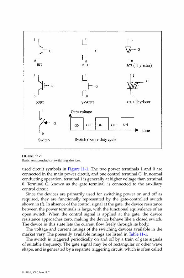
© 1999 by CRC Press LLC
used circuit symbols in Figure 11-1. The two power terminals 1 and 0 areconnected in the main power circuit, and one control terminal G. In normalconducting operation, terminal 1 is generally at higher voltage than terminal0. Terminal G, known as the gate terminal, is connected to the auxiliarycontrol circuit.
Since the devices are primarily used for switching power on and off asrequired, they are functionally represented by the gate-controlled switchshown in (f). In absence of the control signal at the gate, the device resistancebetween the power terminals is large, with the functional equivalence of anopen switch. When the control signal is applied at the gate, the deviceresistance approaches zero, making the device behave like a closed switch.The device in this state lets the current flow freely through its body.
The voltage and current ratings of the switching devices available in themarket vary. The presently available ratings are listed in Table 11-1.
The switch is triggered periodically on and off by a train of gate signalsof suitable frequency. The gate signal may be of rectangular or other waveshape, and is generated by a separate triggering circuit, which is often called
FIGURE 11-1
Basic semiconductor switching devices.

© 1999 by CRC Press LLC
the firing circuit. Although it has a distinct identity and many differentdesign features, it is generally incorporated in the main power electroniccomponent assembly.
In wind power system operating at variable speed for maximum annualenergy production, the output frequency and voltage of the induction gen-erator vary with the wind speed. The variable-frequency, variable-voltageoutput is converted into fixed voltage 60 Hz or 50 Hz terminal output tomatch with utility requirement. In modern plants, this is accomplished bypower electronics scheme shown in Figure 11-2. The variable frequency isfirst rectified into DC, and the DC is then inverted back into the fixedfrequency AC. The increase in the energy production from the variable speedwind turbine over the plant life more than offsets the added cost of the powerelectronics.
In photovoltaic power systems, the DC power produced by the pv modulesis inverted into 60 or 50 Hz AC power using the inverter. The inverter circuitin the pv system is essentially the same that is used in the variable speedwind power system.
The main power electronic components of the wind and pv power systemsare, therefore, the rectifier and the inverter. Their circuits and the AC andDC voltage and current relationships are presented in the following sections.
TABLE 11-1
Maximum Voltage and Current Ratings of Power Electronic Switching Devices
DeviceVoltage Rating,
VoltsCurrent Rating,
Amperes Remark
BJT 1500 200 Requires large current signal to turn onIGBT 1200 100 Combines the advantages of BJT,
MOSFET and GTOMOSFET 1000 100 Higher switching speedSCR 6000 3000 Once turned on, requires heavy turn-off
circuit
FIGURE 11-2
Variable-speed constant-frequency wind power system schematic.

© 1999 by CRC Press LLC
11.2 AC to DC Rectifier
The circuit diagram of the full-bridge, three-phase, AC to DC rectifier isshown Figure 11-3. The power switch generally used in the rectifier is thesilicon-controlled rectifier. The average DC output voltage in this circuit isgiven by the following:
(11-1)
where V
L
= line-to-line voltage on three-phase AC side of the rectifier
α
= angle of firing delay in the switching.
The delay angle is measured from the zero crossing in the positive half ofthe AC voltage wave. Equation 11-1 shows that the output DC voltage iscontrollable by varying the delay angle
α
, which in turn controls the con-duction (on-time) of the switch.
The load determines the DC side current:
In the steady state operation, the balance of power must be maintainedon both AC and DC sides. That is, the power on the AC side must be equalto the sum of the DC load power and the losses in the rectifier circuit. TheAC side power is therefore:
FIGURE 11-3
Three-phase full bridge AC to DC silicon-controlled rectifier circuit.
V Vdc L=π
3 2cos α
IC
DC = D load powerVDC

© 1999 by CRC Press LLC
(11-2)
Moreover, as we will see in Chapter 14, the three-phase AC power is givenby the following:
(11-3)
where cos
φ
is the power factor on the AC side. With a well-designed powerelectronic converter, the power factor on the AC side is approximately equalto that of the load.
From Equation 11-2 with 11-3, we obtain the AC-side line current I
L
.
11.3 DC to AC Inverter
The power electronic circuit used to convert DC into AC is known as theinverter. The term “converter” is often used to mean either the rectifier orthe inverter. The DC input to the inverter can be from any of the followingsources:
• rectified DC output of the variable speed wind power system.• DC output of the photovoltaic power modules.• DC output of the battery used in the wind or photovoltaic power
system.
Figure 11-4 shows the DC to three-phase AC inverter circuit diagram. TheDC source current is switched successively in a 60 Hz three-phase timesequence such as to power the three-phase load. The AC current containssignificant harmonics as discussed in Section 14-7. The fundamental fre-quency (60 or 50 Hz) phase-to-neutral voltage is as follows:
(11-4)
The line-to-line AC voltage, as will be seen in the next chapter, is givenby · Vph.
Unlike in BJT, MOSFET, and IGBT, the thyristor current, once switched on,must be forcefully switched off (commutated) to cease conduction. If thethyristor is used as the switching device, the circuit must incorporate addi-tional commutating circuit to perform this function. The commutating circuitis a significant part of the inverter circuit. There are two main types ofinverters, the line commutated and the forced commutated.
PC
AC = D load powerrectifier efficiency
P V IAC L L= ⋅ ⋅ ⋅3 cos φ
V Vph DC=π
π
⋅2 2
6cos
3

© 1999 by CRC Press LLC
The line-commutated inverter must be connected to the AC system intowhich they feed power. The design method is matured and has been exten-sively used in the high-voltage DC transmission line inverters. Such invertersare simple and inexpensive and can be designed in any size. The disadvan-tage is that they act as a sink of reactive power and generate high contentof harmonics.
Poor power factor and high harmonic content in line commutated inverterssignificantly degrade the quality of power at the utility interface. This prob-lem has been recently addressed by a series of design changes in the invert-ers. Among them is the 12-pulse inverter circuit and increased harmonicfiltering. These new design features have resulted in today’s inverters oper-ating at near unity power factor and less than 3 to 5 percent total harmonicdistortion. The quality of power at the utility interface at many modern windpower plants exceeds that of the grid they interface.
The force-commutated inverter does not have to be supplying load andcan be free-running as an independent voltage source. The design is rela-tively complex and expensive. The advantage is that they can be a source ofreactive power and the harmonics content is low.
11.4 Grid Interface Controls
At the utility interface, the power flow direction and magnitude depend onthe voltage magnitude and the phase relation of the site voltage with respectto the grid voltage. The grid voltage being fixed, the site voltage must becontrolled both in magnitude and in phase in order to feed power to thegrid when available, and to draw from the grid when needed. If the inverteris already included in the system for frequency conversion, the magnitude
FIGURE 11-4
DC to three-phase AC inverter circuit.

© 1999 by CRC Press LLC
and phase control of the site voltage is done with the same inverter with noadditional hardware cost. The controls are accomplished as follows:
11.4.1 Voltage Control
For interfacing with the utility grid lines, the renewable power system outputvoltage at the inverter terminals must be adjustable. The voltage is controlledby using one of the following two methods:
1. By controlling the alternating voltage output of the inverter usingtap-changing autotransformer at the inverter output (Figure 11-5).The tap changing is automatically obtained in a closed-loop controlsystem. If the transformer has a phase-changing winding also, acomplete control on the magnitude and phase of the site voltagecan be achieved. The advantages of this scheme are that the siteoutput voltage waveshape does not vary over a wide range, andhigh input power factor is achieved by using uncontrolled dioderectifiers for the DC link voltage. The added cost of the transformer,however, can be avoided by using the method discussed below.
2. Since the magnitude of the alternating voltage output from thestatic inverter is proportional to the direct voltage input from therectifier, the voltage control can be achieved by operating theinverter with the variable DC link voltage. Such a system alsomaintains the same output voltage, frequency and wave shape overa wide range. However, in circuits deriving the load current fromthe commutating capacitor voltage from the DC link, the commu-tating capability decreases when the output voltage is reduced.This could lead to an operational difficulty when the DC link volt-age varies over a wide range, such as in motor drives controlling
FIGURE 11-5
Voltage control by means of uncontrolled rectifier and variable ratio tap-changing transformer.

© 1999 by CRC Press LLC
the speed in ratio exceeding four to one. In renewable power appli-cations, such commutation difficulty is unlikely as the speed variesover a narrow range.
The variable DC link voltage is obtained two ways:
• one way is to connect a variable ratio transformer on the input sideof the rectifier. The secondary tap changing is automaticallyobtained in a closed-loop control system.
• the other way is to use the phase-controlled rectifier in place of theuncontrolled rectifier in Figure 11-5. At reduced output voltage,this method gives poor power factor and high harmonic content,and requires filtering the DC voltage before feeding to the inverter.
11.4.2 Frequency Control
The output frequency of the inverter solely depends on the rate at whichthe switching thyristors or transistors are triggered into conduction. Thetriggering rate is determined by the reference oscillator producing a contin-uous train of timing pulses, which are directed by logic circuits to the thy-ristor gating circuits. The timing pulse train is also used to control the turn-off circuits. The frequency stability and accuracy requirements of the inverterdictate the selection of the reference oscillator. A simple temperature com-pensated R-C relaxation oscillator gives the frequency stability within0.02 percent. When better stability is needed, a crystal-controlled oscillatorand digital counters may be used, which can provide stability of .001 percentor better. The frequency control in a stand-alone power system is an open-loop system. The steady state or transient load changes do not affect thefrequency. This is one of the major advantages of the power electronicsinverter over the old electromechanical means of frequency controls.
11.5 Battery Charge/Discharge Converters
The stand-alone photovoltaic power system uses the DC to DC converterfor battery charging and discharging.
11.5.1 Battery Charge Converter
Figure 11-6 is the most widely used DC-DC battery charge converter circuit,also called the buck converter. The switching device used in such convertersmay be the BJT, MOSFET, or the IGBT. The buck converter steps down theinput bus voltage to the battery voltage during battery charging. The tran-sistor switch is turned on and off at high frequency (in tens of kHz). Theduty ratio D of the switch is defined as the following:
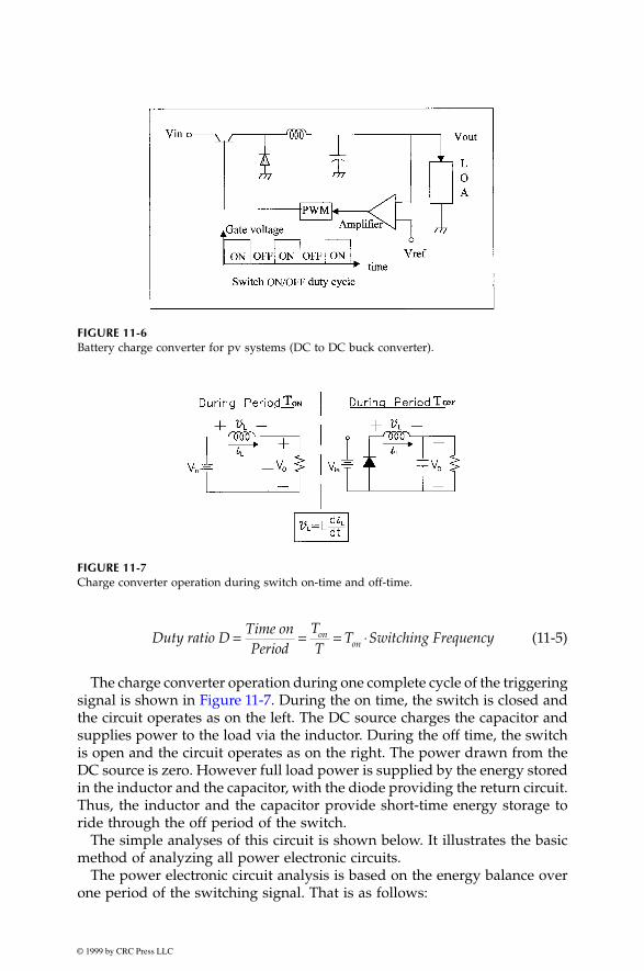
© 1999 by CRC Press LLC
(11-5)
The charge converter operation during one complete cycle of the triggeringsignal is shown in Figure 11-7. During the on time, the switch is closed andthe circuit operates as on the left. The DC source charges the capacitor andsupplies power to the load via the inductor. During the off time, the switchis open and the circuit operates as on the right. The power drawn from theDC source is zero. However full load power is supplied by the energy storedin the inductor and the capacitor, with the diode providing the return circuit.Thus, the inductor and the capacitor provide short-time energy storage toride through the off period of the switch.
The simple analyses of this circuit is shown below. It illustrates the basicmethod of analyzing all power electronic circuits.
The power electronic circuit analysis is based on the energy balance overone period of the switching signal. That is as follows:
FIGURE 11-6
Battery charge converter for pv systems (DC to DC buck converter).
FIGURE 11-7
Charge converter operation during switch on-time and off-time.
Duty ratio DTime onPeriod
Switching Frequency= = = ⋅TT
Tonon

© 1999 by CRC Press LLC
Energy supplied to the load over the total period of repetition.= Energy drawn from the source during the on-time, and
Energy supplied to the load during the off-time= Energy drawn from the inductor and the capacitor during off-time
Alternatively, the volt-second balance method is used, which in essence givesthe energy balance.
The voltage and current waveforms are displayed in Figure 11-8. In thesteady state condition, the inductor volt-second balance during the on andoff periods must be maintained. Since the voltage across the inductor mustequal L dI
L
/dt,
During on-time, (11-6)
And during off-time (11-7)
If the inductor is large enough, as usually is the case in practical circuits,the change in the inductor current is small, and the peak value of the inductorcurrent is given by the following:
FIGURE 11-8
Current and voltage waveforms in the buck converter.
∆I L V V TL in out on⋅ = −( ) ⋅
∆I L V TL out off⋅ = ⋅

© 1999 by CRC Press LLC
(11-8)
where the load current I
o
= V
out
/R
load
= average value of the inductor current.
The algebraic manipulation of the above equations leads to the following:
(11-9)
It is seen from Equation 11-9 that the output voltage is controlled byvarying the duty ratio D. This is done in a feedback control loop with therequired battery charge current as the reference. The duty ratio is controlledby modulating the pulse width of T
on
. Such a converter is, therefore, alsoknown as the Pulse Width Modulated (PWM) converter.
11.5.2 Battery Discharge Converter
The battery discharge converter circuit is shown in Figure 11-9. It steps upthe sagging battery voltage during discharge to the required output voltage.When the transistor switch is on, the inductor is connected to the DC source.When the switch is off, the inductor current is forced to flow through thediode and the load. The output voltage of the boost converter is derivedagain from the volt-second balance in the inductor. With duty ratio D of theswitch, the output voltage is given by the following:
(11-10)
For all values of D < 1, the output voltage is always greater than the inputvoltage. Therefore, the boost converter can only step up the voltage. On the
FIGURE 11-9
Battery discharge converter circuit for pv systems (DC to DC boost converter).
I I Ipeak o L= + 12 ∆
V V Dout in= ⋅
VV
Doutin=
−1

© 1999 by CRC Press LLC
other hand, the buck converter presented in the preceding section can onlystep down the input voltage. Combining the two converters in cascade,therefore, give a buck-boost converter, which can step down or step up theinput voltage. A modified buck-boost converter often used for this purposeis shown in Figure 11-10. The voltage relation is obtained by cascading thebuck and boost converter voltage relations. That is as follows:
(11-11)
Equation 11-11 for the buck-boost converter shows that the output voltagecan be higher or lower than the input voltage depending on the duty ratio D(Figure 11-11).
In addition to its use in the battery charging and discharging, the buck-boost circuit is capable of four-quadrant operation with the DC machine
FIGURE 11-10
Buck-boost converter circuit (general DC to DC converter for pv systems).
FIGURE 11-11
Buck-boost converter output to input ratio versus duty ratio.
VV D
Doutin=
⋅−1
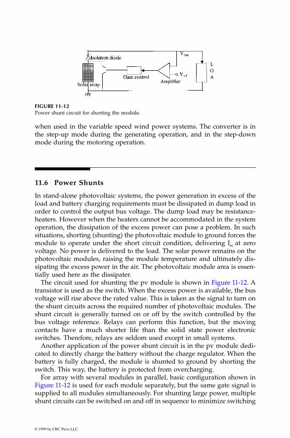
© 1999 by CRC Press LLC
when used in the variable speed wind power systems. The converter is inthe step-up mode during the generating operation, and in the step-downmode during the motoring operation.
11.6 Power Shunts
In stand-alone photovoltaic systems, the power generation in excess of theload and battery charging requirements must be dissipated in dump load inorder to control the output bus voltage. The dump load may be resistance-heaters. However when the heaters cannot be accommodated in the systemoperation, the dissipation of the excess power can pose a problem. In suchsituations, shorting (shunting) the photovoltaic module to ground forces themodule to operate under the short circuit condition, delivering I
sc
at zerovoltage. No power is delivered to the load. The solar power remains on thephotovoltaic modules, raising the module temperature and ultimately dis-sipating the excess power in the air. The photovoltaic module area is essen-tially used here as the dissipater.
The circuit used for shunting the pv module is shown in Figure 11-12. Atransistor is used as the switch. When the excess power is available, the busvoltage will rise above the rated value. This is taken as the signal to turn onthe shunt circuits across the required number of photovoltaic modules. Theshunt circuit is generally turned on or off by the switch controlled by thebus voltage reference. Relays can perform this function, but the movingcontacts have a much shorter life than the solid state power electronicswitches. Therefore, relays are seldom used except in small systems.
Another application of the power shunt circuit is in the pv module dedi-cated to directly charge the battery without the charge regulator. When thebattery is fully charged, the module is shunted to ground by shorting theswitch. This way, the battery is protected from overcharging.
For array with several modules in parallel, basic configuration shown inFigure 11-12 is used for each module separately, but the same gate signal issupplied to all modules simultaneously. For shunting large power, multipleshunt circuits can be switched on and off in sequence to minimize switching
FIGURE 11-12
Power shunt circuit for shorting the module.

© 1999 by CRC Press LLC
transients and electromagnetic interference (EMI) with the neighboringequipment. For fine power control, one segment can be operated in the pulsewidth modulation (PWM) mode.
The power electronics is a very wide and developing subject. The intentof this chapter is to present an overview of the basic circuits used in thewind and photovoltaic power systems. Further details can be obtained frommany excellent books on power electronics.
1-3
References
1. Bose, B. “Power Electronics and Variable Frequency Drives,”
IEEE Press,
1996.2. Dewan, S. B. and Straughen, A. 1975. “Power Semiconductor Circuits,” New
York, John Wiley
&
Sons, 1975.3. Mohan, N. and Undeland, T. 1995. “Power Electronics Converters, Applications
and Design,” IEEE and John Wiley & Sons, 1995.

© 1999 by CRC Press LLC
12
Stand-Alone System
The major application of the stand-alone power system is in remote areaswhere utility lines are uneconomical to install due to terrain, the right-of-way difficulties or the environmental concerns. Even without these con-straints, building new transmission lines is expensive. A 230 kV line costsabout $1 million per mile. For remote villages farther than two miles fromthe nearest transmission line, a stand-alone wind system could be moreeconomical. The break-even distance for pv systems, however, is longerbecause the pv energy is four to five times more expensive than wind energyat present.
The solar and wind power outputs can fluctuate on an hourly or dailybasis. The stand-alone system must, therefore, have some means of storingenergy, which can be used later to supply the load during the periods of lowor no power output. Alternatively, the wind or pv or both can also be usedin a hybrid configuration with diesel engine generator in remote areas orwith fuel cells in urban areas.
According to the World Bank, more than 2 billion people live in villagesthat are not yet connected to utility lines. These villages are the largestpotential market of the hybrid stand-alone systems using diesel generatorwith wind or pv for meeting their energy needs. Additionally, the wind andpv systems create more jobs per dollar invested, which help minimize themigration to already strained cities.
Because power sources having differing performance characteristics mustbe used in parallel, the stand-alone hybrid system is technically more chal-lenging and expensive to design than the grid-connected system that simplyaugments the existing utility system.
12.1 pv Stand-Alone
The typical pv stand-alone system consists of a solar array and a batteryconnection as shown in Figure 12-1. The array powers the load and chargesthe battery during daytime. The battery powers the load after dark. The

© 1999 by CRC Press LLC
inverter converts the DC power of the array and the battery into 60 or 50 Hzpower. Inverters are available in a wide range of power ratings with effi-ciency ranging from 85 to 95 percent. The array is segmented with isolationdiodes for improving the reliability. In such designs, if one string of the solararray fails, it does not load or short the remaining strings. Multiple inverters,such as three inverters each with 35 percent rating rather than one with105 percent rating, are preferred. If one such inverter fails, the remaining twocan continue supplying essential loads until the failed one is repaired orreplaced. The same design approach also extends in using multiple batteries.
Most of the stand-alone pv systems installed in developing countries pro-vide basic necessities, such as lighting and pumping water. Others go a stepfurther (Figure 12-2).
12.2 Electric Vehicle
The solar electric car developed in the U.S.A. and in many other countriesis an example of the stand-alone (rather the move-alone) pv power system.The first solar car was built in 1981 and driven across the Australian Outbackby Hans Tholstrup of Australia. The solar car has been developed and iscommercially available, although more expensive than the conventional carat present. However, the continuing development is closing the price-gapevery year.
A new sport at the American universities these days is the annual solarcar race. The DOE and several car manufacturers sponsor the race every twoyears. It is open to all engineering and business students, who design, build,and run their car across the heartland of America. The first U.S. solar carrace was organized in 1990. Figure 12-3 shows one such car built by theUniversity of Michigan. In 1993, it finished first in the 1,100-mile “Sunrayce”that began from Arlington, Texas, and cruised through Oklahoma, Kansas,Missouri, Iowa and ended in Minnesota. It covered 1,102 miles in six and a
FIGURE 12-1
Photovoltaic stand-alone power system with battery.
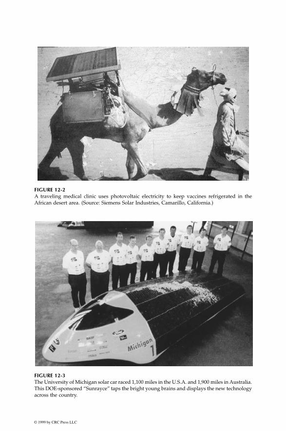
© 1999 by CRC Press LLC
FIGURE 12-2
A traveling medical clinic uses photovoltaic electricity to keep vaccines refrigerated in theAfrican desert area. (Source: Siemens Solar Industries, Camarillo, California.)
FIGURE 12-3
The University of Michigan solar car raced 1,100 miles in the U.S.A. and 1,900 miles in Australia.This DOE-sponsored “Sunrayce” taps the bright young brains and displays the new technologyacross the country.

© 1999 by CRC Press LLC
half days. In 1994, the Michigan car finished the 1,900-mile long World SolarChallenge from Darwin to Adelaide across the Australian Outback. Severaldozens of teams participate in the race. Much more than just a race, the goalof this DOE program is to provide the hands-on, minds-on experience toyoung students in renewable power sources, and display it on the wheelsacross the country.
The solar cars entering the “Sunrayce” every year generally have a widerange of the design characteristics as listed in Table 12-1. The Michigan carwas designed with silicon cells and lead-acid battery, which was changedto the silver-zinc battery later on. With a permanent magnet brushless DCmotor, it reached the peak speed of 50 miles per hour. The Gallium arsenidepv cells are often used in the Australian race, but are not allowed in the U.S.race. A few race cars have been designed with a sterling engine driven byhelium heated by the solar energy instead of using the photovoltaic cells.The design considerations include trading hundreds of technical parameterscovered throughout this book and making decisions to meet the constraints.But certain key elements are essential for winning. They are as follows:
• photovoltaic cells with high conversion efficiency.• peak power tracking design.• lightweight battery with high specific energy.• energy efficient battery charging and discharging.• low aerodynamic drag.• high reliability without adding weight.
The zinc-air battery discussed in Chapter 10 is an example of a lightweightbattery. Chapter 8 covered the use of isolation diodes in solar array forachieving the reliability without adding weight, and the peak power trackingprinciple for extracting the maximum power output under the given solarradiation.
After the car is designed and tested, the strategy to optimize the solarenergy capture and to use it efficiently while maintaining the energy balancefor the terrain and the weather on the day of the race becomes the final test
TABLE 12-1
Design Characteristic Range of Solar Cars Built by U.S. University Students
for the Biennial 1,100-Mile ‘Sunrayce’
Design Parameters Parameter Range
Solar array power capability (silicon crystalline, gallium arsenide)
750–1500 watts
Battery (Lead-acid, Silver-Zinc) 3.5–7 kWhElectric motor (DC brushless with permanent magnet) 4–8 horsepowerCar weight 500–1000 poundsCar dimensions (approximate overall)
≈
20’ long
×
7’ wide
×
3.5’ high
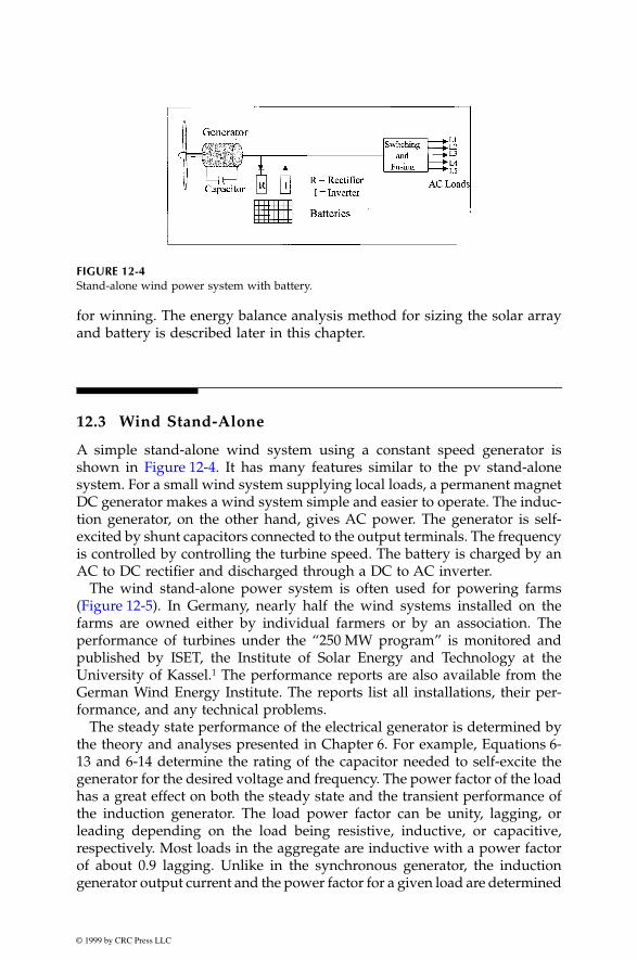
© 1999 by CRC Press LLC
for winning. The energy balance analysis method for sizing the solar arrayand battery is described later in this chapter.
12.3 Wind Stand-Alone
A simple stand-alone wind system using a constant speed generator isshown in Figure 12-4. It has many features similar to the pv stand-alonesystem. For a small wind system supplying local loads, a permanent magnetDC generator makes a wind system simple and easier to operate. The induc-tion generator, on the other hand, gives AC power. The generator is self-excited by shunt capacitors connected to the output terminals. The frequencyis controlled by controlling the turbine speed. The battery is charged by anAC to DC rectifier and discharged through a DC to AC inverter.
The wind stand-alone power system is often used for powering farms(Figure 12-5). In Germany, nearly half the wind systems installed on thefarms are owned either by individual farmers or by an association. Theperformance of turbines under the “250 MW program” is monitored andpublished by ISET, the Institute of Solar Energy and Technology at theUniversity of Kassel.
1
The performance reports are also available from theGerman Wind Energy Institute. The reports list all installations, their per-formance, and any technical problems.
The steady state performance of the electrical generator is determined bythe theory and analyses presented in Chapter 6. For example, Equations 6-13 and 6-14 determine the rating of the capacitor needed to self-excite thegenerator for the desired voltage and frequency. The power factor of the loadhas a great effect on both the steady state and the transient performance ofthe induction generator. The load power factor can be unity, lagging, orleading depending on the load being resistive, inductive, or capacitive,respectively. Most loads in the aggregate are inductive with a power factorof about 0.9 lagging. Unlike in the synchronous generator, the inductiongenerator output current and the power factor for a given load are determined
FIGURE 12-4
Stand-alone wind power system with battery.

© 1999 by CRC Press LLC
by the generator parameters. Therefore, when the induction generator deliv-ers a certain load, it also supplies a certain in-phase current and a certainquadrature current. The quadrature current is supplied by the capacitor bankconnected to the terminal. Therefore, the induction generator is not suitablefor supplying low power factor loads.
The transient performance of the stand-alone, self-excited induction gen-erator, on the other hand, is more involved. The generalized d-q axis modelof the generator is required. The computer simulation using the d-q axismodel shows the following general transient characteristics:
2
• under sudden loss of the self-excitation due to tripping-off thecapacitor bank, the resistive and inductive loads cause the terminalvoltage quickly reach the steady state zero. The capacitive loadtakes a longer time before the terminal voltage decays to zero.
• under sudden loading of the generator, the resistive and inductiveloads result in sudden voltage drop, while the capacitive load haslittle effect on the terminal voltage.
• under sudden loss of resistive and inductive loads, the terminalvoltage quickly rises to its steady state value.
• at light load, the magnetizing reactance will change to its unsatur-ated value, which is large. This makes the machine performanceunstable, resulting in the terminal voltage to collapse.
FIGURE 12-5
Remote farms are a major market for the stand-alone power systems. (Source: World PowerTechnologies, Duluth, Minnesota. With permission.)

© 1999 by CRC Press LLC
To remedy the instability problem indicated above, the stand-alone induc-tion generator must always have some minimum load, dummy if necessary,permanently connected to its terminals.
12.4 Hybrid System
12.4.1 Hybrid with Diesel
The certainty of meeting load demands at all times is greatly enhanced bythe hybrid system using more than one power source. Most hybrids usediesel generator with pv or wind, since diesel provides more predictablepower on demand. In some hybrids, batteries are used in addition to thediesel generator. The batteries meet the daily load fluctuation, and the dieselgenerator takes care of the long-term fluctuations. For example, the dieselgenerator is used in the worst case weather condition, such as extendedovercasts or windless days or weeks.
Figure 12-6 is one of the largest pv-diesel hybrid systems installed inCalifornia. The project was part of the Environmental Protection Agency’sPV-Diesel Program.
Figure 12-7 is a schematic layout of the wind/diesel/battery hybrid sys-tem. The power connection and control unit (PCCU) provides a central placeto make organized connections of most system components. In addition, thePCCU houses the following components:
• battery charge and discharge regulators.• transfer switches and protection circuit breakers.• power flow meters.• mode controller.
Figure 12-8 is a commercially available PCCU for hybrid power systems.The transient analysis of the integrated wind-pv-diesel requires an exten-
sive model that takes the necessary input data and event definitions forcomputer simulation.
3
12.4.2 Hybrid with Fuel Cell
In stand-alone renewable power systems of hybrid designs, the fuel cell hasthe potential to replace the diesel engine in urban areas. In these applications,the diesel engine would be undesirables due to its environmental negatives.The airborne emission of fuel cell power plant is 25 grams per MWh delivered.
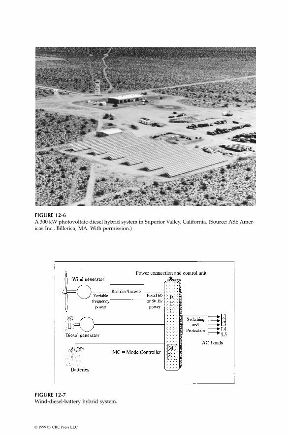
© 1999 by CRC Press LLC
FIGURE 12-6
A 300 kW photovoltaic-diesel hybrid system in Superior Valley, California. (Source: ASE Amer-icas Inc., Billerica, MA. With permission.)
FIGURE 12-7
Wind-diesel-battery hybrid system.

© 1999 by CRC Press LLC
Factories and hospitals have considered the fuel cell to replace the dieselgenerator in the uninterruptible power system. Electric utility companies areconsidering the fuel cell for meeting the peak demand and for load levelingbetween the day and night and during the week.
The fuel cell is an electrochemical device that generates electricity bychemical reaction without altering the electrodes or the electrolyte materials.This distinguishes the fuel call from the electrochemical batteries. The con-cept of the fuel cell is the reverse of the electrolysis of water, in which thehydrogen and oxygen are combined to produce electricity and water. Thefuel cell is a static device that converts the chemical energy directly intoelectrical energy. Since fuel cell bypasses the thermal-to-mechanical conver-sion, and since its operation is isothermal, the conversion efficiency is notCarnot-limited. This way, it differs from the diesel engine.
The fuel cell, developed as an intermediate-term power source for spaceapplications, was first used in a moon buggy and continues to be used topower NASA’s space shuttles. It also finds other niche applications atpresent. Providing electrical power for a few days or a few weeks is notpractical using the battery, but is easily done with the fuel cell.
The basic constructional features of the fuel cell are shown in Figure 12-9.The hydrogen ‘fuel’ is combined with oxygen of the air to produce electricity.The hydrogen, however, does not burn as in the internal combustion engine,rather it produces electrically by an electrochemical reaction. Water and heatare the byproducts of this reaction if the fuel is pure hydrogen. With thenatural gas, ethanol or methanol as the source of hydrogen, the byproductsinclude carbon dioxide, and traces of carbon monoxide, hydrocarbons andnitrogen oxides. However, they are less than 1 percent of those emitted bythe diesel engine. The superior reliability with no moving parts is an addi-tional benefit of the fuel cell over the diesel generator. Multiple fuel cells
FIGURE 12-8
Integrated power connection and control unit for wind-pv-battery hybrid system. (Source:World Power Technologies, Duluth, Minnesota. With permission.)

© 1999 by CRC Press LLC
stack up in series-parallel combinations for the required voltage and current,just as the electrochemical cells do in the battery.
The low temperature (250°C) fuel cell is now commercially available fromseveral sources. It uses phosphoric acid as the electrolytic solution betweenthe electrode plates. A typical low temperature fuel cell with a peak powerrating of 200 kW costs under $1,800 per kW at present, which is over twicethe cost of the diesel engine. The fuel cell price, however, is falling with newdevelopments being implemented every year.
The high temperature fuel cell has a higher power generation capacity perkilogram at a relatively high cost, limiting the use in special applications atpresent. Solid oxide, solid polymer, molten carbonate, and proton membraneexchange fuel cells in this category are being developed. The industry interestin such cells is in large capacity for use in a utility power plant. The FuelCell Commercialization Group in the U.S.A. recently field-tested moltencarbonate direct-fuel cells for 2 MW utility-scale power plants. The testresults were a qualified success. Based on the results, a commercial plant isbeing designed for a target date of operation by the year 2000.
Solid oxide fuel cells of several different designs, consisting of essentiallysimilar materials for the electrolyte, the electrodes, and the interconnections,are being investigated worldwide. Most success to date has been achievedwith the tubular geometry being developed by the Westinghouse Electric
FIGURE 12-9
Fuel cell principle: hydrogen and oxygen in, electrical power and water out.

© 1999 by CRC Press LLC
Corporation in the U.S.A. and Mitsubishi Heavy Industries in Japan. Thecell element in this geometry consists of two porous electrodes separated bya dense oxygen ion-conducting electrolyte as depicted in Figure 12-10.
4
Ituses ceramic tube operating at 1,000°C. The fuel cell is an assembly of suchtubes. SureCELL™ (Trademark of Westinghouse Electric Corporation, Pitts-burgh, Pennsylvania) is a solid oxide high temperature tubular fuel cellshown in Figure 12-11. It is being developed for multi-megawatt combinedcycle gas turbine and fuel cell plants and targeted for distributed powergeneration and cogeneration plants of up to 60 MW capacity. It fits well forutility scale wind and photovoltaic power plants. Inside SureCELL, naturalgas or other fuels are converted to hydrogen and carbon monoxide by inter-nal reformation. No external heat or stream is needed. Oxygen ions producedfrom an air stream react with the hydrogen and carbon monoxide to generateelectric power and high temperature exhaust gas.
Because of the closed-end tubular configuration, no seals are required andrelative cell movement due to differential thermal expansions is not restricted.This enhances the thermal cycle capability. The tubular configuration solvesmany of the design problems facing other high temperature fuel cells. Thetarget for the SureCELL development is to attain 75 percent overall efficiency,compared to 60 percent possible using only the gas turbine (Figure 12-12).Environmentally, the solid oxide fuel cell produces much lower CO
2
, NOxand virtually zero SOx compared with other fuel cell technologies.
During the eight years of failure-free steady state operation of early pro-totypes, these cells were able to maintain the output voltage within0.5 percent per 1,000 hours of operation. The second generation of the West-inghouse fuel cell shows voltage degradation of less then 0.1 percent per1,000 hours of operation, with life in tens of thousands of hours of operation.The SureCELL prototype has been tested for over 1,000 thermal cycles with
FIGURE 12-10
Air electrode supported type tubular solid oxide fuel cell design. (Courtesy of WestinghouseElectric Company, A Division of CBS Corporation, Pittsburgh, PA. Reprinted with permission.)

© 1999 by CRC Press LLC
zero performance degradation, and 12,000 hours of operation with less then1 percent performance degradation.
The transient electrical performance model of the fuel cell includes elec-trochemical, thermal, and mass flow elements that affects the electrical out-put.
5
Of primary interest is the electrical response of the cell to a load change.To design for the worst case, the performance is calculated under both theconstant reactant flow and the constant inlet temperature.
FIGURE 12-11
Seal-less solid oxide fuel cell power generator. (Courtesy of Westinghouse Electric Company,A Division of CBS Corporation, Pittsburgh, PA. Reprinted with permission.)

© 1999 by CRC Press LLC
The German-American car-manufacturer Daimler-Chrysler and BallardPower Systems of Canada are developing the solid polymer fuel cell forautomobiles as an alternative to the battery-powered vehicles. Their targetis to sell the first commercial fuel cell powered car by the year 2004.
12.4.3 Mode Controller
The overall system must be designed for a wide performance range toaccommodate the characteristics of the diesel generator (or fuel cell), thewind generator, and the battery. As and when needed, switching to thedesired mode of generation is done by the mode controller. Thus, the modecontroller is the central monitor and controller of the hybrid systems. Ithouses the microcomputer and software for the source selection, the batterymanagement, and load shedding strategy. The mode controller performs thefollowing functions:
• monitors and controls the health and state of the system.• monitors and controls the battery state-of-charge.• brings up the diesel generator when needed, and shuts off when
not needed.• sheds low priority loads in accordance with the set priorities.
The battery comes on-line by automatic transfer switch, which takes about5 ms to connect to the load. The diesel, on the other hand, is generally brought
FIGURE 12-12
Natural gas power generation system efficiency comparison. (Courtesy of Westinghouse ElectricCompany, A Division of CBS Corporation, Pittsburgh, PA. Reprinted with permission.)

© 1999 by CRC Press LLC
on-line, manually or automatically after going through the preplanned strat-egy algorithm. Even with automatic transfer switches, the diesel generatortakes a long time to come on-line. Typically, this delay time is approximately20 seconds.
The mode controller is designed and programmed with deadbands toavoid change over of the sources for correcting small variation on the busvoltage and frequency. The deadbands avoid chatters in the system.Figure 12-13 is an example of 120 volts hybrid system voltage-controlregions. The deadbands are along the horizontal segments of the control line.
As a part of the overall system controller, the mode controller may incor-porate the maximum power extraction algorithm. The dynamic behaviorsof the closed-loop system, following common disturbances such as insolationchanges due to cloud, wind fluctuation, sudden load changes and shortcircuit faults, are taken into account in a comprehensive design.
6
12.4.4 Load Sharing
Since the wind, pv, battery, and diesel (or fuel cell) in various combinations,operate in parallel, the load sharing between them is one of the key designaspects of the hybrid system. For example, in the wind/diesel hybrid system(Figure 12-14), the electrical properties of the two systems must match sothat they share load in proportion to their rated capacities.
For determining the load sharing, the two systems are first reduced to theirrespective Thevenin equivalent circuit model, in which each system is rep-resented by its internal voltage and the series impedance. This is shown inFigure 12-14. The terminal characteristics of the two generators are thengiven by the following:
(12-1)
where subscripts 1 and 2 represent system 1 and 2 respectively, and
FIGURE 12-13
Mode controller deadbands eliminates the system chatter.
E E I Z
E E I Z
1 01 1 1
2 02 2 2
= − ⋅
= − ⋅⋅
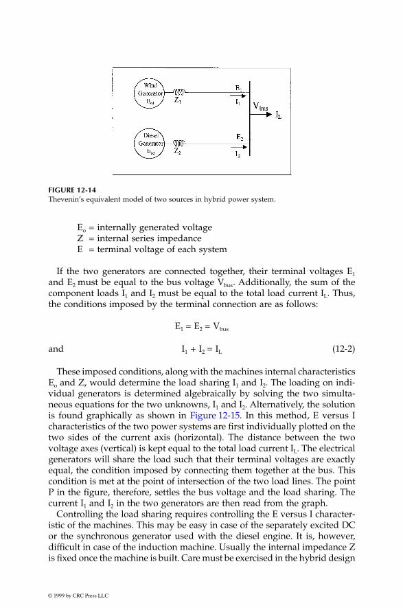
© 1999 by CRC Press LLC
E
o
= internally generated voltageZ = internal series impedanceE = terminal voltage of each system
If the two generators are connected together, their terminal voltages E
1
and E
2
must be equal to the bus voltage V
bus
. Additionally, the sum of thecomponent loads I
1
and I
2
must be equal to the total load current I
L
. Thus,the conditions imposed by the terminal connection are as follows:
E
1
= E
2
= V
bus
and I
1
+ I
2
= I
L
(12-2)
These imposed conditions, along with the machines internal characteristicsE
o
and Z, would determine the load sharing I
1
and I
2
. The loading on indi-vidual generators is determined algebraically by solving the two simulta-neous equations for the two unknowns, I
1
and I
2
. Alternatively, the solutionis found graphically as shown in Figure 12-15. In this method, E versus Icharacteristics of the two power systems are first individually plotted on thetwo sides of the current axis (horizontal). The distance between the twovoltage axes (vertical) is kept equal to the total load current I
L
. The electricalgenerators will share the load such that their terminal voltages are exactlyequal, the condition imposed by connecting them together at the bus. Thiscondition is met at the point of intersection of the two load lines. The pointP in the figure, therefore, settles the bus voltage and the load sharing. Thecurrent I
1
and I
2
in the two generators are then read from the graph.Controlling the load sharing requires controlling the E versus I character-
istic of the machines. This may be easy in case of the separately excited DCor the synchronous generator used with the diesel engine. It is, however,difficult in case of the induction machine. Usually the internal impedance Zis fixed once the machine is built. Care must be exercised in the hybrid design
FIGURE 12-14
Thevenin’s equivalent model of two sources in hybrid power system.

© 1999 by CRC Press LLC
to make sure that sufficient excitation control is built in for the desired loadsharing between the two sources.
The load sharing strategy can vary depending on the priority of loads andthe cost of electricity from alternative sources. In a wind-diesel system, forexample, diesel electricity is generally more expensive than wind (~25 versus5 cents per kWh). Therefore, all priority-1 (essential) loads are met first bywind as far as possible and then by diesel. If the available wind power ismore than priority-1 loads, wind supplies part of priority-2 loads and thediesel is not run. If the wind power now fluctuates on the down side, thelower priority loads are shed to avoid running the diesel. If wind powerdrops further to cut into the priority-1 load, the diesel is brought on-lineagain. Water pumping and heater loads are examples of priority-2 loads.
12.5 System Sizing
For determining the required capacity of the stand-alone power system,estimating the peak load demand is only one aspect of the design. Estimatingthe energy required over the duration selected for the design is the firstrequirement for the system sizing.
12.5.1 Power and Energy Estimates
The system sizing starts with compiling a list of all loads that are to beserved. Not all loads are constant. Time-varying loads are expressed in peakwatts they consume and the duty ratio. The peak power consumption isused in determining the wire size for making a connection to the source.
FIGURE 12-15
Graphical determination of load shared by two sources in hybrid power system.

© 1999 by CRC Press LLC
The duty ratio is used in determining the contribution of individual load inthe total energy demand. If the load has clean on-off periods as shown inFigure 12-16(a), then the duty ratio D is defined as D = To/T, where To isthe time the load is on and T is the period of repetition. For irregularlyvarying loads shown in (b), the duty ratio is defined as the actual energyconsumed in one period over the peak power times the period, i.e.:
(12-3)
The peak power consumption and the duty ratio of all loads are compiled,the product of the two is the actual share of the energy requirement of thatload on the system during one repetition period. If there are distinct intervalsin the period, say between the battery discharge and charge intervals, thenthe peak power and the duty ratio of each load are computed over the twointervals separately. As a simple example of this in a solar power system,one interval may be from 8
A
.
M
. to 6
P
.
M
. and the other from 6
P
.
M
. to 8
A
.
M
.The power table is then prepared as shown in Table 12-2.
FIGURE 12-16
Duty ratio and peak power of intermittent loads.
TABLE 12-2
Power and Energy Compilation Table for Energy Balance Analysis
8
A
.
M
. to 6
P
.
M
. (Interval A)
(battery on charge)6
P
.
M
. to 8
A
.
M
. (Interval B)
(battery on discharge)
LoadPeak watts
Duty ratio
Energy per period Wh
Peak watts
Duty ratio
Energy per period Wh
Load
1
P
1a
D
1a
E
1a
P
1b
D
1b
E
1b
Load
2
P
2a
D
2a
E
2a
P
2b
D
2b
E
2b
. . . . . . . . . . . . . .Load
n
P
na
D
na
E
na
P
nb
D
nb
E
nb
TOTAL
Σ
P
a
Σ
E
a
Σ
P
b
Σ
E
b
Total Battery Discharge Required =
Σ
E
b
watts-hours
D = ⋅⋅
Energy in watt hours consumed in one repetition periodPeak power in watts Repetition period in hours

© 1999 by CRC Press LLC
In a community of homes and businesses, not all connected loads drawpower simultaneously. The statistical time staggering in their use timesresults in the average power capacity requirement of the plant significantlylower than the sum of the individually connected loads. The National Elec-trical Code
®
provides factors for determining the average community loadin normal residential and commercial areas (Table 12-3). The average plantcapacity is then determined as follows:
Required power system capacity = NEC
®
factor from Table 12-3
×
Sum of connected loads.
12.5.2 Battery Sizing
The battery Ah capacity required to support the load energy requirement ofE
bat
as determined using a method of Table 12-2 or equivalent:
(12-4)
where
E
bat
= energy required from the battery per discharge
η
disch
= efficiency of discharge path, including inverters, diodes,wires, etc.
N
cell
= number of series cells in one battery
V
disch
= average cell voltage during discharge
DOD
allowed
= maximum DOD allowed for the required cycle life
N
bat
= number of batteries in parallel
The following example illustrates the use of this formula to size the battery.Suppose we want to design a battery for a stand-alone power system, whichcharges and discharges the battery from 110 volts DC solar array. For the
TABLE 12-3
NEC
®
Demand Factors (Adapted from National Electrical Code
®
Handbook,
7
th
Edition, 1996, Table 220-32)
Number of Dwellings Demand Factor
3 0.4510 0.4315 0.4020 0.3825 0.3530 0.3340 0.2850 0.26
>62 0.23
AhE
N V DoD Nbat
disch cell disch allowed bat
=⋅[ ] ⋅ ⋅η

© 1999 by CRC Press LLC
DC-DC buck converter that charges the battery, the maximum availablebattery-side voltage is 70 volts for it to work efficiently in the PWM mode.For the DC-DC boost converter discharging the battery, the minimumrequired battery voltage is 45 volts. Assuming that we are using NiMHbattery, the cell voltage can vary from 1.55 when fully charged to 1.1 whendrained to the maximum allowable DOD. Then, the number of cells neededin the battery is less than 70/1.55 = 45 cells and more than 45/1.1 = 41. Thus,the number of cells required in the battery from the voltage considerationsis between 41 and 45. It is generally more economical to use fewer cells ofhigher capacity than more lower-capacity cells. We, therefore, select 41 cellsin the battery design.
Now again for an example, let us assume that the battery is required todischarge 2 kW load for 14 hours (28,000 Wh) every night for five yearsbefore replacement. The life requirement is, therefore, 5
×
365 = 1,825 cyclesof deep discharge. For the NiMH battery, the cycle life at full depth ofdischarge is 2,000. Since this is greater than the 1,825 cycles required, we canfully discharge the battery every night for five years. If the discharge effi-ciency is 80 percent, the average cell discharge voltage is 1.2 V, and we desirethree batteries in parallel for reliability, each battery Ah capacity calculatedfrom the above equation is as follows:
(12-5)
Three batteries, each having 41 series cells of 237 Ah capacity, therefore,will meet the system requirement. Margin must be allowed to account forthe uncertainty in estimating the loads.
12.5.3 pv Array Sizing
The basic tenet in sizing the stand-alone “power system” is to rememberthat it is really the stand-alone “energy system.” It must, therefore, maintainthe energy balance over the specified period. The energy drained duringlean times must be made up by the positive balance during the remainingtime of the period. A simple case of a constant load on the pv system usingsolar arrays perfectly pointing toward the sun normally for 10 hours of theday is shown in Figure 12-17 to illustrate the point. The solar array is sizedsuch that the two shaded areas on two sides of the load line must be equal.That is, the area
oagd
must be equal to the area
gefb
. The system losses inthe round trip energy transfers, e.g., from and to the battery, adjust theavailable load to a lower value as shown by the dotted line.
In general, the stand-alone system must be sized so as to satisfy the fol-lowing energy balance equation over one period of repetition.
Ah =⋅ ⋅[ ]⋅ ⋅
=280000 80 41 1 2 1 0 3
237. . .
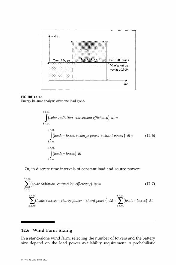
© 1999 by CRC Press LLC
(12-6)
Or, in discrete time intervals of constant load and source power:
12.6 Wind Farm Sizing
In a stand-alone wind farm, selecting the number of towers and the batterysize depend on the load power availability requirement. A probabilistic
FIGURE 12-17
Energy balance analysis over one load cycle.
solar radiation conversion efficiency
loads losses charge power shunt power
⋅( ) ⋅ =
+ + +( ) ⋅ +
+( ) ⋅
∫
∫
∫
dt
dt
loads losses dt
A M
P M
A M
P M
P M
A M
8
6
8
6
6
8
. .
. .
. .
. .
. .
. .
solar radiation conversion efficiency
loads losses charge power
⋅( ) ⋅ =
+ + +( ) ⋅ + +( ) ⋅
∑
∑ ∑
∆
∆ ∆
t
shunt power t loads losses t
A M
P M
A M
P M
P M
A M
8
6
8
6
6
8
. .
. .
. .
. .
. .
. .
(12-7)
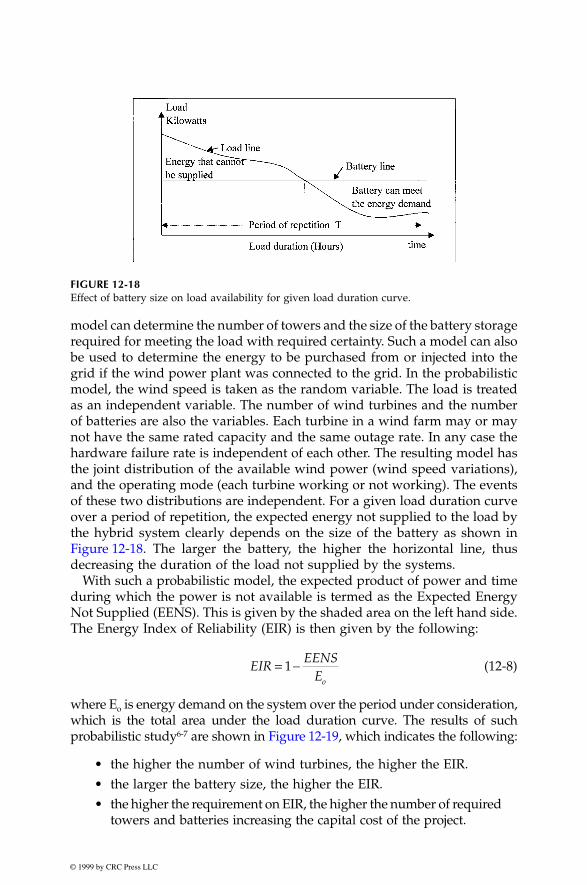
© 1999 by CRC Press LLC
model can determine the number of towers and the size of the battery storagerequired for meeting the load with required certainty. Such a model can alsobe used to determine the energy to be purchased from or injected into thegrid if the wind power plant was connected to the grid. In the probabilisticmodel, the wind speed is taken as the random variable. The load is treatedas an independent variable. The number of wind turbines and the numberof batteries are also the variables. Each turbine in a wind farm may or maynot have the same rated capacity and the same outage rate. In any case thehardware failure rate is independent of each other. The resulting model hasthe joint distribution of the available wind power (wind speed variations),and the operating mode (each turbine working or not working). The eventsof these two distributions are independent. For a given load duration curveover a period of repetition, the expected energy not supplied to the load bythe hybrid system clearly depends on the size of the battery as shown inFigure 12-18. The larger the battery, the higher the horizontal line, thusdecreasing the duration of the load not supplied by the systems.
With such a probabilistic model, the expected product of power and timeduring which the power is not available is termed as the Expected EnergyNot Supplied (EENS). This is given by the shaded area on the left hand side.The Energy Index of Reliability (EIR) is then given by the following:
(12-8)
where E
o
is energy demand on the system over the period under consideration,which is the total area under the load duration curve. The results of suchprobabilistic study
6-7
are shown in Figure 12-19, which indicates the following:
• the higher the number of wind turbines, the higher the EIR.• the larger the battery size, the higher the EIR.• the higher the requirement on EIR, the higher the number of required
towers and batteries increasing the capital cost of the project.
FIGURE 12-18Effect of battery size on load availability for given load duration curve.
EIREENS
Eo
= −1
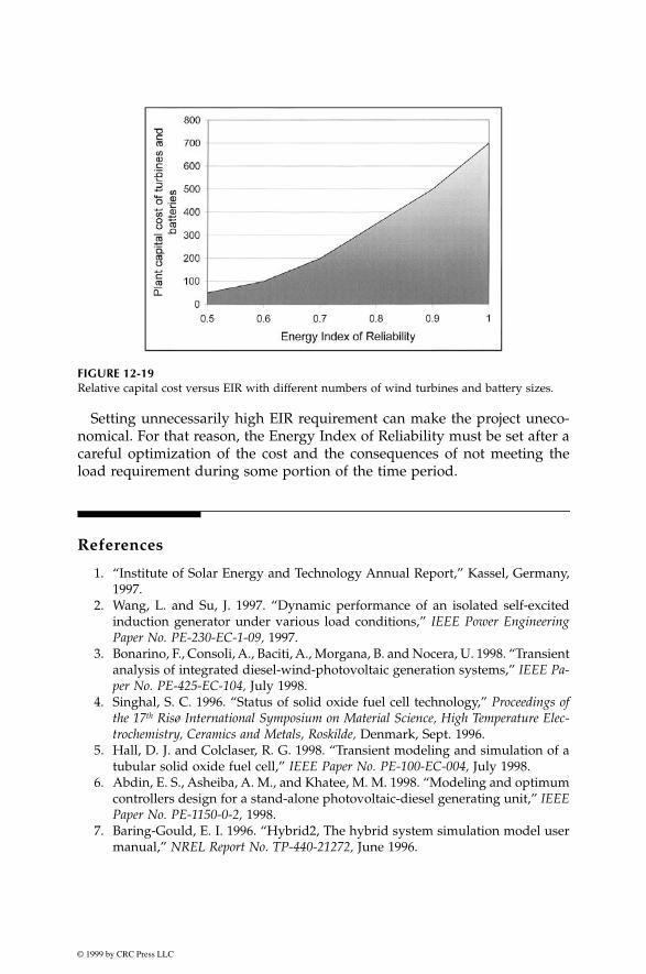
© 1999 by CRC Press LLC
Setting unnecessarily high EIR requirement can make the project uneco-nomical. For that reason, the Energy Index of Reliability must be set after acareful optimization of the cost and the consequences of not meeting theload requirement during some portion of the time period.
References
1. “Institute of Solar Energy and Technology Annual Report,” Kassel, Germany,1997.
2. Wang, L. and Su, J. 1997. “Dynamic performance of an isolated self-excitedinduction generator under various load conditions,” IEEE Power EngineeringPaper No. PE-230-EC-1-09, 1997.
3. Bonarino, F., Consoli, A., Baciti, A., Morgana, B. and Nocera, U. 1998. “Transientanalysis of integrated diesel-wind-photovoltaic generation systems,” IEEE Pa-per No. PE-425-EC-104, July 1998.
4. Singhal, S. C. 1996. “Status of solid oxide fuel cell technology,” Proceedings ofthe 17th Risø International Symposium on Material Science, High Temperature Elec-trochemistry, Ceramics and Metals, Roskilde, Denmark, Sept. 1996.
5. Hall, D. J. and Colclaser, R. G. 1998. “Transient modeling and simulation of atubular solid oxide fuel cell,” IEEE Paper No. PE-100-EC-004, July 1998.
6. Abdin, E. S., Asheiba, A. M., and Khatee, M. M. 1998. “Modeling and optimumcontrollers design for a stand-alone photovoltaic-diesel generating unit,” IEEEPaper No. PE-1150-0-2, 1998.
7. Baring-Gould, E. I. 1996. “Hybrid2, The hybrid system simulation model usermanual,” NREL Report No. TP-440-21272, June 1996.
FIGURE 12-19Relative capital cost versus EIR with different numbers of wind turbines and battery sizes.

© 1999 by CRC Press LLC
13
Grid-Connected System
The wind and photovoltaic power systems have made a successful transitionfrom small stand-alone sites to large grid-connected systems. The utilityinterconnection brings a new dimension in the renewable power economyby pooling the temporal excess or the shortfall in the renewable power withthe connecting grid. This improves the overall economy and the load avail-ability of the renewable plant; the two important factors of any power sys-tem. The grid supplies power to the site loads when needed, or absorbs theexcess power from the site when available. One kWh meter is used to recordthe power delivered to the grid, and another kWh meter is used to record thepower drawn from the grid. The two meters are generally priced differently.
Figure 13-1 is a typical circuit diagram of the grid-connected photovoltaicpower system. It interfaces with the local utility lines at the output side ofthe inverter as shown. A battery is often added to meet short term load peaks.In the United States, the Environmental Protection Agency sponsors grid-connected pv programs in urban areas where wind towers would be imprac-tical. In recent years, large building-integrated photovoltaic installations havemade significant advances by adding the grid-interconnection in the systemdesign. Figure 13-2 shows the building-integrated pv system on the roof ofthe Northeastern University Student Center in Boston, MA. The project waspart of the EPA PV DSP Program. The system produces 18 kW pv power andis connected to the grid. In addition, it collects sufficient research data usingnumerous instruments and computer data loggers. The vital data are sampledevery 10 seconds, and then are averaged and stored every 10 minutes. Theincoming data includes information about the air temperature and windspeed. The performance parameters include the DC voltage and current gen-erated by the pv roof, and the AC power on the inverter output side.
In the United Kingdom, a 390 square meter building-integrated pv systemhas been in operation since 1995 at the University of Northumbria, Newcastle(Figure 13-3). The system produces 33,000 kWh electricity per year and isconnected to the grid. The pv panels are made of monocrystalline cells withthe photoconversion efficiency of 14.5 percent.
On the wind side, most grid-connected systems are large utility-scalepower plants. A typical equipment layout in such plants is shown inFigure 13-4. The wind generator output is at 480 volts AC, which is raised

© 1999 by CRC Press LLC
to an intermediate level of 21 kV by a pad-mounted transformer. An over-head transmission line provides the link to the site substation, where thevoltage is raised again to the grid level. The site computer, sometimes usingmulitplexer and remote radio links, controls the wind turbines in responseto the wind conditions and the load demand.
FIGURE 13-1
Electrical schematic of the grid-connected photovoltaic system.
FIGURE 13-2
18 kW grid-connected pv system on the Northeastern University Student Center in Boston,MA. (Source: ASE Americas, Billerica, Massachusetts. With permission.)

© 1999 by CRC Press LLC
FIGURE 13-3
Grid-connected pv system at the University of Northumbria, Newcastle, U.K. The 390 squaremeter monocrystalline modules produce 33,000 kWh per year. (Source: Professional Engineer,Publication of the Institution of Mechanical Engineer’s, London. With permission.)

© 1999 by CRC Press LLC
Large wind systems being installed now tend to have the variable-speeddesign. The power schematic of such a system is shown in Figure 13-5. Thevariable-frequency generator output is first rectified into DC, and theninverted into a fixed-frequency AC. Before the inversion, the rectifier har-monics are filtered out from the DC by the inductor and capacitors. Thefrequency reference for the inverter firing and the voltage reference for therectifier phase-angle control are taken from the grid lines. The optimumreference value of the tip-speed ratio is stored and continuously compared
FIGURE 13-4
Electrical component layout of the grid-connected wind power system. (Source: AWEA/IEA/CADDET Technicla Brochure, 1995.)
FIGURE 13-5
Electrical schematic of the grid-connected variable speed wind power system.

© 1999 by CRC Press LLC
with the value computed from the measured speeds of the wind and therotor. The turbine speed is accordingly changed to assure maximum powerproduction at all times.
13.1 Interface Requirements
Both the wind and the pv systems interface the grid at the output terminalsof the synchronizing breaker at the output end of the inverter. The powerflows in either direction depending on the site voltage at the breaker termi-nals. The fundamental requirements on the site voltage for interfacing withthe grid are as follows:
• the voltage magnitude and phase must equal to that required forthe desired magnitude and direction of the power flow. The voltageis controlled by the transformer turn ratio and/or the recti-fier/inverter firing angle in a closed-loop control system.
• the frequency must be exactly equal to that of the grid, or else thesystem will not work. To meet the exacting frequency requirement,the only effective means is to use the utility frequency as a referencefor the inverter switching frequency.
• in the wind system, the synchronous generators of the grid systemsupply magnetizing current for the induction generator.
The interface and control issues are similar in many ways between boththe pv and the wind systems. The wind system, however, is more involvedsince the electrical generator and the turbine with large inertia introducecertain dynamic issues not applicable in the static pv system. Moreover, windplants generally have much greater power capacity than the pv plants. Forexample, many wind plants that have been already installed around theworld have capacity in tens of MW each. The newer wind plants in thehundreds of MW capacity are being installed and more are planned.
13.2 Synchronizing with Grid
The synchronizing breaker in Figures 13-1 and 13-5 has internal voltage andphase angle sensors to monitor the site and grid voltages and signal thecorrect instant for closing the breaker. As a part of the automatic protectioncircuit, any attempt to close the breaker at an incorrect instant is rejected bythe breaker. Four conditions which must be satisfied before the synchroniz-ing switch will permit the closure are as follows:

© 1999 by CRC Press LLC
• the frequency must be as close as possible with the grid frequency,preferably about one-third of a hertz higher.
• the terminal voltage magnitude must match with that of the grid,preferably a few percent higher.
• the phase sequence of the two three-phase voltages must be thesame.
• the phase angle between the two voltages must be within 5 degrees.
Taking the wind power system as an example, the synchronizing processspecifically runs as follows:
1. With the synchronizing breaker open, the wind power generatoris brought up to speed using the machine in the motoring mode.
2. Change the machine into the generating mode, and adjust thecontrols such that the site and grid voltages match to meet theabove requirements as close as possible.
3. The match is monitored by the synchroscope or three synchroniz-ing lamps, one in each phase (Figure 13-6). The voltage across the
FIGURE 13-6
Synchronizing circuit using three synchronizing lamps or the synchroscope.

© 1999 by CRC Press LLC
lamp in each phase is the difference between the renewable sitevoltage and the grid voltage at any instant. When the site and thegrid voltages are exactly equal in all three phases, all three lampswill be dark. However, it is not enough for the lamps to be darkat any one instant. They must remain dark for a long time. Thiscondition which will be met only if the generator and the gridvoltages have nearly the same frequency. If not, one set of the twothree-phase voltages will rotate faster relative to the other, and thephase difference between the two voltages will light the lamps.
4. The synchronizing breaker is closed if the lamps remain dark for to second.
Following the closure, any small mismatch between the site voltage andthe grid voltage will circulate the inrush current between the two such thatthe two systems will come to perfect synchronous operation.
13.2.1 Inrush Current
The small unavoidable difference between the site and the grid voltages willresult in an inrush current to flow between the site and the grid. The inrushcurrent eventually decays to zero at an exponential rate that depends on theinternal resistance and inductance. The initial magnitude of this current inthe instant the circuit breaker is closed depends on the degree of mismatchbetween the two voltages. It is not all bad, as it produces the synchronizingpower which acts to bring the two systems in synchronous lock. However,it produces a mechanical torque step, setting up the electromechanical oscil-lations before the two machines come into synchronism and get locked witheach other. The magnitude of the inrush current is calculated as follows:
Let
∆
V be the difference between the site voltage and the grid voltage atthe closing instant due to any reason. Since this voltage is suddenly appliedon the system, the resulting inrush current is determined by the subtransientreactance of the machine
X
d
″
. That is as follows:
(13-1)
The inrush current is primarily reactive, as is solely determined by
X
d
″
. Itsmagnitude is kept within the allowable limit, else the thermal or mechanicaldamage may result.
The synchronizing power produced by the inrush current brings the windsystem and the grid in synchronism after the oscillations decay out. Oncesynchronized, the generator has a natural tendency to remain in synchronismwith the grid, although it can fall out of synchronization if excessive load isextracted, large load steps are applied, or during system faults. Small per-turbation swings in the load angle decay out over a time, restoring the
14⁄ 12⁄
IV
Xinrushd
=′′
∆
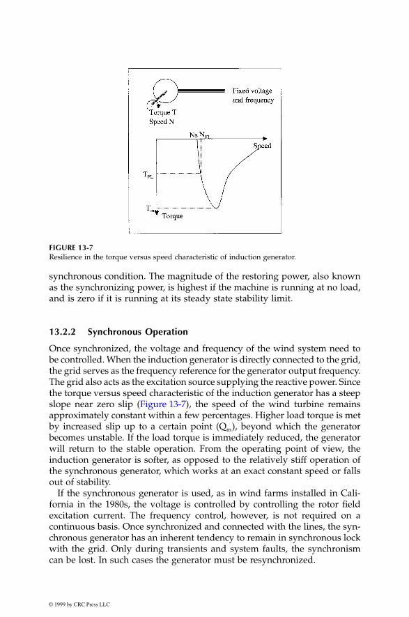
© 1999 by CRC Press LLC
synchronous condition. The magnitude of the restoring power, also knownas the synchronizing power, is highest if the machine is running at no load,and is zero if it is running at its steady state stability limit.
13.2.2 Synchronous Operation
Once synchronized, the voltage and frequency of the wind system need tobe controlled. When the induction generator is directly connected to the grid,the grid serves as the frequency reference for the generator output frequency.The grid also acts as the excitation source supplying the reactive power. Sincethe torque versus speed characteristic of the induction generator has a steepslope near zero slip (Figure 13-7), the speed of the wind turbine remainsapproximately constant within a few percentages. Higher load torque is metby increased slip up to a certain point (Q
m
), beyond which the generatorbecomes unstable. If the load torque is immediately reduced, the generatorwill return to the stable operation. From the operating point of view, theinduction generator is softer, as opposed to the relatively stiff operation ofthe synchronous generator, which works at an exact constant speed or fallsout of stability.
If the synchronous generator is used, as in wind farms installed in Cali-fornia in the 1980s, the voltage is controlled by controlling the rotor fieldexcitation current. The frequency control, however, is not required on acontinuous basis. Once synchronized and connected with the lines, the syn-chronous generator has an inherent tendency to remain in synchronous lockwith the grid. Only during transients and system faults, the synchronismcan be lost. In such cases the generator must be resynchronized.
FIGURE 13-7
Resilience in the torque versus speed characteristic of induction generator.
© 1999 by CRC Press LLC
In the variable-speed induction generator system using the inverter at theinterface, the inverter gate signal is derived from the grid voltage to assuresynchronism. The inverter stability depends a great deal on the design. Forexample, with line commutated inverter, there is no stability limit. The powerlimit in this case is the steady state load limit of the inverter with any short-term overload limit.
13.2.3 Load Transient
During steady state operation, if the renewable power system output is fullyor partially lost, the grid will pick up the area load. The effect of this willbe felt in two ways:
• the grid generators slow down slightly to increase their powerangle needed to make up for the lost power. This will result in amomentary drop in frequency.
• small voltage drop results throughout the system, as the grid con-ductors carry more load.
The same effects are felt if a large load is suddenly switched in at the greenpower site, starting the wind turbine as the induction motor draws a largecurrent. This will result in the above effect. Such load transients are mini-mized by soft-starting large generators. In wind farms consisting of manygenerators, individual generators are started in sequence, one after another.
13.2.4 Safety
Safety is a concern when renewable power is connected to the utility gridlines. The interconnection may endanger the utility repair crew working onthe lines by continuing to feed power into the grid even when the grid itselfwent down. This issue has been addressed by including an internal circuitthat takes the inverter off line immediately if the system detects grid outage.Since this circuit is critical for human safety, it has a built-in redundancy.
The site-grid interface breaker can get suddenly disconnected, accidentallyor to meet an emergency situation. The high wind speed cut out is a usualcondition when the power is cut off to protect the generator from overload-ing. In systems where large capacitors are connected at the wind site forpower factor improvement, the site generator would still be in the self-excitation mode, drawing excitation power from the capacitors and gener-ating terminal voltage. In absence of such capacitors, one would assume thatthe voltage at the generator terminals would come down to zero. The linecapacitance, however, can keep the generator self excited. The protectioncircuit is designed to avoid both of these situations, which are potential safetyhazards to unsuspecting site crew.

© 1999 by CRC Press LLC
When the grid is disconnected for any reason, the generator will experiencea loss of frequency regulation, as the frequency synchronizing signal derivedfrom the grid lines is now lost. When a change in frequency is detectedbeyond a certain limit, the automatic control can shut down the system,cutting off all possible sources of excitation.
13.3 Operating Limit
The link line connecting the renewable power site with the utility gridintroduces the operating limit in two ways, the voltage regulation and thestability limit. In most cases, the line can be considered as an electricallyshort transmission line. The ground capacitance and the ground leakageresistance are generally negligible and are ignored. The equivalent circuit ofsuch a line, therefore, reduces to a series resistance R and reactance L(Figure 13-8). Such an approximation is valid in lines up to 50 miles long.The line carries power from the renewable site to the utility grid, or fromthe grid to the renewable site to meet local peak demand. There are twomajor effects of the transmission line impedance, one on the voltage regu-lation and the other on the maximum power transfer capability of the linkline.
13.3.1 Voltage Regulation
The phasor diagram of the voltage and current at the sending and receivingends are shown in Figure 13-9. Since the shunt impedance is negligible, thesending end current I
s
is the same as the receiving end current I
r
, i.e., I
s
=I
r
= I. The voltage at the receiving end is the vector sum of the sending endvoltage plus the impedance voltage drop I·Z in the line, i.e.:
FIGURE 13-8
Equivalent circuit of renewable power plant connected to grid via transmission line link.

© 1999 by CRC Press LLC
(13-2)
The voltage regulation is defined as the rise in the receiving end voltage,expressed in percent of the full load voltage, when full load at a specifiedpower factor is removed, holding the sending end voltage constant. That isas follows:
(13-3)
where V
nl
= magnitude of receiving end voltage at no load = V
s
V
fl
= magnitude of receiving end voltage at full load = V
r
With reference to the phasor diagram of Figure 13-9, V
nl
= V
s
and V
fl
= V
r
.The voltage regulation is a strong function of the load power factor. For
the same load current at different power factors, the voltage drop in the lineis the same, but is added to the sending end voltage at different phase anglesto derive the receiving end voltage. For this reason, the voltage regulationis greater for lagging power factor, and the least or even negative for leadingpower factor.
In Figure 13-9, suppose the magnitude of V
r
and I are held constant andthe power factor of the load is varied from zero lagging to zero leading. Thevector V
s
will vary such that its end point will lie on a semicircle since themagnitude I · (R + jX) is constant.
1
Such a circle diagram is useful for plottingthe sending end voltage versus load power factor for the given load voltageand KVA.
FIGURE 13-9
Phasor diagram of the link line carrying rated current.
V V I R jXs r= + +( )
percent voltage regulation =−
×V V
Vnl fl
fl
100

© 1999 by CRC Press LLC
If the voltages at both ends of the lines are held constant in magnitude,the receiving end real power and reactive power points plotted for severalloads would lie on a circle known as the power circle diagram. The readeris referred to Stevenson
1
for further reading on the transmission line circlediagrams.
13.3.2 Stability Limit
The direction of the power flow depends on the sending and receiving endvoltages, and the electrical phase angle between the two. However, themaximum power the line can transfer while maintaining stable operationhas a limit. We derive below the stability limit assuming that the powerflows from the renewable power site to the grid, although the same limitapplies in the reverse direction as well. The series resistance in most lines isnegligible, hence, is ignored here.
The power transferred to the grid by the transmission line is as follows:
(13-4)
Using the phasor diagram of Figure 13-9, the current I can be expressedas follows:
(13-5)
The real part of this current is as follows:
(13-6)
This, when multiplied with the receiving end voltage Vr, gives the follow-ing power:
(13-7)
Thus, the magnitude of the real power transferred by the line depends onthe power angle
δ
. If
δ
> 0, the power flows from the site to the grid. On theother hand, if
δ
< 0, the site draws power from the grid.The reactive power depends on (Vs–Vr). If Vs > Vr, the reactive power
flows from the site to the grid. If Vs < Vr, the reactive power flows from thegrid to the site.
P V Ir= cos φ
ddP
P kP P L kP
P L kP
o
o
η =+( ) − + +( )
+ +( )=
1 20
2
2 2
IV
Xreals=⋅ sinδ
PV V
Xs r=⋅
sinδ
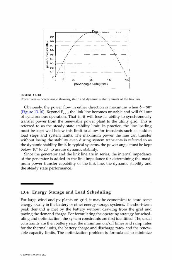
© 1999 by CRC Press LLC
Obviously, the power flow in either direction is maximum when
δ
= 90°(Figure 13-10). Beyond P
max
, the link line becomes unstable and will fall outof synchronous operation. That is, it will lose its ability to synchronouslytransfer power from the renewable power plant to the utility grid. This isreferred to as the steady state stability limit. In practice, the line loadingmust be kept well below this limit to allow for transients such as suddenload steps and system faults. The maximum power the line can transferwithout losing the stability even during system transients is referred to asthe dynamic stability limit. In typical systems, the power angle must be keptbelow 10° to 20° to assure dynamic stability.
Since the generator and the link line are in series, the internal impedanceof the generator is added in the line impedance for determining the maxi-mum power transfer capability of the link line, the dynamic stability andthe steady state performance.
13.4 Energy Storage and Load Scheduling
For large wind and pv plants on grid, it may be economical to store someenergy locally in the battery or other energy storage systems. The short-termpeak demand is met by the battery without drawing from the grid andpaying the demand charge. For formulating the operating strategy for sched-uling and optimization, the system constraints are first identified. The usualconstraints are then battery size, the minimum on/off times and ramp ratesfor the thermal units, the battery charge and discharge rates, and the renew-able capacity limits. The optimization problem is formulated to minimize
FIGURE 13-10
Power versus power angle showing static and dynamic stability limits of the link line.

© 1999 by CRC Press LLC
the cost of all thermal and renewable units combined subject to the con-straints by arriving at the best short-term scheduling. This determines thehours for which the baseload thermal units of the electrical power companyshould be taken either off-line or on-line. The traditional thermal schedulingalgorithms, augmented Lagrangian relaxation, branch and bound, successivedynamic programming or heuristic method (genetic algorithms and neuralnetworks), can be used for minimizing the cost of operating the thermalunits with a given renewable-battery system. Marwali et al.
2
has recentlyutilized the successive dynamic programming to find the minimum costtrajectory for battery and the augmented Langrangian to find thermal unitcommitment. In a case study of a 300 MW thermal-pv-battery power plant,the authors have arrived at the total production costs shown in Table 13-1,where the battery hybrid system saves $54,000 per day compared to thethermal only.
13.5 Utility Resource Planning Tool
The wind and photovoltaic power, in spite of their environmental, financial,and fuel diversity benefits, are not presently included in the utility resourceplanning analysis because of the lack of the familiarity and analytical toolsfor nondispatchable sources of power. The wind and pv powers are treatedas nondispatchable for not being available on demand. The MassachusettsInstitute of Technology’s Energy Laboratory has developed an analytical toolto analyze the impact of nondispatchable renewables on the New England’spower systems operation. Cardell and Connors
3
have applied this tool foranalyzing two hypothetical wind farms totaling 1,500 MW capacity for twosites, one in Maine and the other in Massachusetts. The average capacityfactor at these two sites is estimated to be 0.25. This is good, although somesites in California have achieved the capacity factor of 0.33 or higher. TheMIT study shows that the wind energy resource in New England is compa-rable to that in California. The second stage of their analysis developed theproduct cost model, demonstrating the emission and fuel cost risk mitigationbenefits of the utility resource portfolios incorporating the wind power.
TABLE 13-1
Production Cost of 300 MW Thermal-pv-Battery System
System ConfigurationBattery Depletion
MWh/dayProduction cost
$/daySavings
$/day
Thermal only — 750,000 —Thermal + pv — 710,000 40,000Thermal + pv + battery 344 696,000 54,000

© 1999 by CRC Press LLC
References
1. Stevenson, W. D. 1962. “Elements of Power System Analysis,” New York,McGraw Hill Book Company, 1962.
2. Marwali, M. K. C., Halil, M., Shahidehpour, S. M., and Abdul-Rahman, K. H.1997. “Short-term generation scheduling in photovoltaic-utility grid with bat-tery storage,”
IEEE paper No. PE-184-PWRS-16-09,
1997.3. Cardell, J. B. and Connors, S. R. 1997. “Wind power in New England, modeling
and analyses of nondispatchable renewable energy technologies,”
IEEE PaperNo. PE-888-PWRS-2-06,
1997.

© 1999 by CRC Press LLC
14
Electrical Performance
14.1 Voltage Current and Power Relations
The power systems worldwide are 60 Hz or 50 Hz AC three-phase systems.The three coils (phases) of the generator are connected in Y or
∆
as shownin Figure 14-1. In the balanced three-phase operation, the line-to-line voltage,the line current and the three phase power in terms of the phase voltage andcurrent are given by the following equations, with notations marked inFigure 14-1.
In the Y connected system:
(14-1)
Where pf = power factorIn the
∆
connected system:
(14-2)
For steady state or dynamic performance studies, the system componentsare modeled so as to represent the entire system. The power generator, therectifier, the inverter, and the battery models were discussed in the earlierchapters. The components are accurately modeled to represent the conditionsunder which the performance is to be determined. This chapter concernsitself with the system level performance.
V V
I I
P V I pf
L ph
L ph
ph L L
=
=
=−
3
33
V V
I I
P V I pf
L ph
L ph
ph L L
=
=
=−
3
33

© 1999 by CRC Press LLC
One-line diagram is widely used to represent the three phases of thesystem. Figure 14-2 is an example of a one-line diagram of the grid-connectedsystem. On the left hand side are two Y-connected synchronous generators,one grounded through a reactor and one grounded through a resistor, sup-plying power to load A. On the right hand side is the wind power site withone
∆
-connected induction generator, supplying power to load B, feedingthe remaining power to the grid via the step up transformer, the circuitbreakers, and the transmission line.
The balanced three-phase system is analyzed as the single-phase system.The neutral wire in the Y connection does not enter the analysis in any way,since it is at zero voltage and carries zero current.
FIGURE 14-1
Three-phase AC systems is connected in Y or
∆
.
FIGURE 14-2
One-line schematic diagram of grid-connected wind farm.

© 1999 by CRC Press LLC
The unbalanced system, the balanced three-phase voltage on unbalancedload and faults need advanced analytical methods, such as the methodsymmetrical components.
14.2 Component Design for Maximum Efficiency
An important performance criterion of any system is the efficiency, measuredas the power output as percentage of the power input. Since the system isas efficient as its components are, designing an efficient system meansdesigning each component to operate at its maximum efficiency.
The electrical and electronic components while transferring power fromthe input side to the output side lose some power in the form of heat. Inpractical designs, the maximum efficiency of 90 to 98 percent is typical inlarge power equipment in hundreds of kW ratings, and 80 to 90 percent insmall equipment in tens of kW ratings. The component efficiency, however,varies with load as shown in Figure 14-3. The efficiency increases with loadup to a certain point beyond which it decreases. A good design maximizesthe efficiency at the load that the equipment supplies most of the time. Forexample, if the equipment is loaded at 70 percent of its rated capacity mostof the time, it is beneficial to have the maximum efficiency at 70 percent load.The method of achieving the maximum efficiency at a desired load level ispresented below.
The total loss in any power equipment generally has two components.One remains fixed representing the quiescent no-load power consumption.The fixed loss primarily includes the eddy and hysteresis losses in the magnetic
FIGURE 14-3
Power equipment efficiency varies with load with single maximum.

© 1999 by CRC Press LLC
parts. The other component varies with the current squared, representingthe I
2
R loss in the conductors. For a constant voltage system, the conductorloss varies with the load power squared. The total loss is, therefore, expressedas (Figure 14-4) the following:
(14-3)
where P is the power delivered to the load (output), L
o
is the fixed loss andk is the proportionality constant. The efficiency is given by the following:
(14-4)
For the efficiency to be maximum at a given load, its derivative with respectto the load power must be zero at that load. That is as follows:
(14-5)
This equation reduces to
L
o
=
kP
2
. Therefore, the component efficiency ismaximum at the load under which the fixed loss is equal to the variable loss.This is an important design rule, which can save significant electrical energyin large power systems.
FIGURE 14-4
Loss components varying with load in typical power equipment.
Loss L k Po= + ⋅ 2
η = =+
=+ +
outputinput
outputoutput loss
PP L kPo
2
ddP
P kP P L kP
P L kP
o
o
η =+( ) − + +( )
+ +( )=
1 20
2
2 2

© 1999 by CRC Press LLC
14.3 Electrical System Model
The electrical network of any complexity can be reduced to a simple Thev-enin’s equivalent circuit consisting of a single source voltage V
s
and imped-ance Z
s
in series (Figure 14-5). The two parameters are determined as follows:With the system operating at no load with all other parameters at rated
values, the voltage at the open-circuit terminals equals the internal sourcevoltage, since the internal voltage drop is zero. Therefore:
V
s
= open-circuit voltage of the system.
For determining the source impedance, the terminals are shorted togetherand the terminal current is measured. Since the internal voltage is nowconsumed in driving the current through the only source impedance, then:
Z
s
= open-circuit voltage/short-circuit current (14-6)
If Z
s
is to be determined by an actual test, the general practice is to shortthe terminals with the open-circuit voltage only several percentages of therated voltage. The low level short-circuit current is measured and the fullshort-circuit current is calculated by scaling to the full-rated voltage. Anynonlinearality, if present, is accounted for.
The equivalent circuit is developed on a per phase basis and in percent orperunit bases. The source voltage, current, and the impedance are expressedin units of their respective base values at the terminal. The base values aredefined as follows:
FIGURE 14-5
Thevenin’s equivalent circuit model of a complex power system.

© 1999 by CRC Press LLC
V
base
= Rated output voltageI
base
= Rated output current, andZ
base
= Rated output voltage/Rated output current
14.4 Static Bus Impedance and Voltage Regulation
If the equivalent circuit model of Figure 14-5 is derived under the steadystate static condition, the Z
s
is called the static bus impedance. The steadystate voltage rise on removal of the full load rated current is then
∆
V = I
base
·Z
s
, and the voltage regulation is as follows:
(14-7)
Under a load step transient, partial or full, as in the case of a loss of loaddue to accidental opening of the load side breaker, the voltage oscillates untilthe transient settles to the new steady state value. If the load current risesin step as shown in Figure 14-6, the voltage goes through oscillation beforesettling down to a lower steady state value. The steady state change in thebus voltage is then given by the following:
∆
V
=
∆
I
·
Z
S
FIGURE 14-6
Transient response of the system voltage under sudden load step.
Voltage Regulation = ⋅∆VVbase
100 percent

© 1999 by CRC Press LLC
The feedback voltage control system responds to bring the bus voltagedeviation back to the rated value. However, in order not to flutter the systemmore than necessary, the control system is designed with suitable deadbands.For example, Figure 14-7 shows a 120 voltage photovoltaic system withbattery with two deadbands in its control system.
14.5 Dynamic Bus Impedance and Ripple
If the circuit model of Figure 14-5 is derived under the dynamic condition,that is for an incremental load, the source impedance is called the dynamicbus impedance, and is denoted by Z
d
. It can be either calculated or measuredas follows. With the bus in operational mode supplying the rated load, injecta small high frequency AC current I
h
into the bus using an independentgrounded current source (Figure 14-8). The high frequency voltage pertur-bation in the bus voltage is measured and denoted by V
h
. The dynamic busimpedance at that frequency is then:
(14-8)
The ripple is the term used to describe periodic glitches in the current orthe voltage, generally of high frequency. Ripples are commonly found insystems with power electronics components, such as rectifiers, inverters,battery chargers, or other switching circuits. The ripples are caused by the
FIGURE 14-7
Deadbands in the feedback voltage control system avoid the system flutter.
ZVId
h
h
=

© 1999 by CRC Press LLC
transistors switching on and off. The ripple frequencies are integer multiplesof the switching frequency. The ripples are periodic but not sinewave andare superimposed on the fundamental wave.
The ripple voltage induced on the bus due to ripple current is given bythe following:
(14-9)
The ripple is minimized by the capacitor connected to the bus or preferablyat the load terminals of the component causing ripples. The ripple currentis then supplied or absorbed by the capacitor, rather than by the bus, thus,improving the quality of power.
14.6 Harmonics
The harmonics is the term used to describe the higher frequency sinewavecurrents or voltages superimposed on the fundamental sinewave. Phase-controlled power switching is one source of harmonics. The harmonics arealso generated by magnetic saturation in power equipment. With no satu-ration present in the magnetic circuit, the generator and the transformerbehave linearly, but not so with saturation. The saturated magnetic circuitrequires non-sinewave magnetizing current.
The usual method of analyzing the system with harmonics is to determinethe performance of the system for each harmonics separately and then tosuperimpose the results. The system is represented by the equivalent circuitfor each harmonic.
The fundamental equivalent circuit of the electrical generator is repre-sented by the d-axis and q-axis.
1-2
In the n
th
harmonic equivalent circuit, the
FIGURE 14-8
Harmonic and dynamic source impedance test measurement set-up.
V I Zripple ripple d= ⋅

© 1999 by CRC Press LLC
harmonic inductance L
n
, being for high frequency, is the average of thesubtransient inductance in the d and q axes, that is as follows:
(14-10)
and the reactance for the harmonic of order n is given by the following:
(14-11)
where f
n
= n
th
harmonic frequencyf = fundamental frequency.
In single-phase or three-phase AC currents having positive and negativeportions of the cycle symmetrical, the odd number of harmonics are absent.That is, I
n
= 0 for n = 2, 4, 6, 8, and so on. In three-phase load circuits fed bytransformers having the primary windings connected in delta, all tripleharmonics are absent in the line currents, that is I
n
= 0 for n = 3, 9, 15, andso on.
In the inverter circuit having m-pulse full bridge circuit, the harmonicspresent are of the order n = mk ± 1, where k = 1, 2, 3, 4, and so on. Forexample, the harmonics present in a 6-pulse inverter are 5, 7, 11, 13, 17, 19.On the other hand, the harmonics present in 12-pulse inverter are 11, 13, 23,25. The magnitude and phase of the harmonic currents are found to beinversely proportional to the harmonic order n, that is as follows:
(14-12)
where I
1
is the fundamental current. This formula gives approximate har-monic contents in 6 and 12-pulse inverters as given in the first two columnsof Table 14-1, which clearly shows the benefits of using 12-pulse converters.
TABLE 14-1
Harmonic Contents of the 6-pulse and 12-pulse Converters
Harmonic Order
n
6-Pulse ConverterEq. 14-12
12-Pulse ConverterEq.14-12
3-pulse and 6-pulse Converters
(IEEE Standard 519)
5 20 — 17.57 14.5 — 11.1
11 9.1 9.1 4.513 7.7 7.7 2.917 5.9 5.9 1.519 5.3 5.3 1.0
LL L
nd q=′′+ ′′( )
2
X f L nfLn n n n= π ⋅ = π2 2
IInn = 1

© 1999 by CRC Press LLC
The actually measured harmonic currents are lower than those given bythe approximate Equation 14-12. The IEEE Standard-519 gives the currentharmonic spectrum in typical 6-pulse converters as listed in the last columnof Table 14-1.
The harmonic currents induce harmonic voltage on the bus. The harmonicvoltage of order n is given by V
n
= I
n
· Z
n
, where Z
n
is the n
th
harmonicimpedance. The harmonic impedance can be derived in a manner similar tothe dynamic impedance, in that a harmonic current I
h
is injected to or drawnfrom the bus and the resulting harmonic voltage V
n
is measured. In a rectifiercircuit drawing harmonic currents I
n
provides a simple circuit which worksas the harmonic current load. If all harmonic currents are measured, thenthe harmonic impedance of order n is given by the following:
(14-13)
14.7 Quality of Power
The requirement of the quality of power at the grid interface is a part of thepower purchase contracts between the utility and the renewable power plant.The rectifier and inverter are the main components contributing to the powerquality concerns. The grid-connected power systems, therefore, need con-verters which are designed to produce high quality, low distortion AC poweracceptable for purchase by the utility company. The power quality concernsbecome more pronounced when the renewable power system is connectedto small capacity grids using long low voltage link.
Until recently, there was no generally acceptable definition of the qualityof power. However, the International Electrotechnical Commission and theNorth American Reliability Council have developed working definitions,measurements and design standards.
Broadly, the power quality has three major components for measurements:
• the total harmonic distortion generated by the power electronicequipment, such as rectifier and inverter.
• the transient voltage sags caused by system disturbances and faults.• periodic voltage flickers.
14.7.1 Harmonic Distortion
Any non-sinusoidal alternating voltage V(t) can be decomposed in the fol-lowing Fourier series:
(14-14)
Z V I where n mk and k and so on.n n n= = ± =, , , , ,1 1 2 3
V t V t V n tn nn( ) = + +( )
=
∞∑1 2sin sinω ω α

© 1999 by CRC Press LLC
The first component on the right hand side of the above equation is thefundamental component, whereas all other higher frequency terms (n =2,3…
∞
) are the harmonics.The Total Harmonic Distortion Factor is defined as follows:
(14-15)
The THD is useful in comparing the quality of AC power at variouslocations of the same power system, or of two or more power systems. In apure sine wave AC source, THD = 0. The greater the value of THD, the moredistorted the sinewave, resulting in more I
2
R loss for the same useful powerdelivered. This way the quality of power and the efficiency are related.
As seen earlier, the harmonic distortion on the bus voltage caused byharmonic current I
n
drawn by any nonlinear load is given by V
n
= I
n
Z
n
. It isthis distortion in the bus voltage that causes the harmonic current to floweven in pure linear resistive load, called the victim load. If the renewablepower plant is relatively small, the nonlinear electronic loads may causesignificant distortion on the bus voltage, which then supplies distorted cur-rent to the linear loads. The harmonics must be filtered out before feedingpower to the grid. For a grid interface, having the THD less than 3 percentis generally acceptable. The IEEE Standard-519 limits the THD for the utilitygrade power to less than 5 percent.
It can be seen that harmonics do not contribute to delivering useful power,but produce I
2
R heating. Such heating in generators, motors, and transform-ers is more difficult to dissipate due to their confined designs, as opposedto open conductors. The 1996 National Electrical Code
®
requires all distri-bution transformers to state their k-ratings on the permanent nameplate.This is useful in sizing the transformer for use in a system having a largeTHD. The k-rated transformer does not eliminate line harmonics. The k-rat-ing merely represents the transformer’s ability to tolerate the distortion. Theunity k rating means the transformer can handle the rated load drawingpure sinewave current. The transformer supplying only electronic load mayrequire high k-rating of 15 to 20.
A recent study funded by the Electrical Power Research Institute reports theimpact of two pv solar parks on the power quality of the grid-connecteddistribution system
3
. The harmonic current and voltage waveforms were mon-itored under connection/disconnection tests over a nine month period endingMarch 1996. The current injected by the pv park had a total distortion belowthe 12 percent limit set by the IEEE-519-1992 standard. However, even theindividual harmonic components between 18 and 48, except the 34
th
, exceededthe IEEE-519 standard. The total voltage distortion, however, was minimal.
A rough measure of quality of power is the ratio of the peak to rms voltagemeasured by the true rms voltmeter. In a pure sine wave, this ratio is =1.414. Most acceptable bus voltages will have this ratio in the 1.3 to 1.5 range,
THDV V V
Vn=
+ +……[ ]22
32 2
12
1
2

© 1999 by CRC Press LLC
which can be used as a quick approximate check on the quality of power atany location in the system.
14.7.2 Voltage Transients and Sags
The bus voltage can deviate from the nominally-rated value due to manyreasons. The deviation that can be tolerated depends on its magnitude andthe time duration. Small deviations can be tolerated for a longer time thanlarge deviations. The tolerance band is generally defined by voltage versustime (v-t) limits. Computers and business equipment using microelectroniccircuits are more susceptible to the voltage transients than the rugged powerequipment such as motors and transformers. The power industry has devel-oped an array of protective equipment. Even then, some standard of powerquality must be maintained at the system level. For example, the systemvoltage must be maintained within the v-t envelope shown in Figure 14-9,where the solid line is that specified by the American National StandardInstitute (ANSI). The right hand side of the band comes primarily from thesteady state performance limitations of motors and transformer-like loads,the middle portion comes from visible lighting flicker annoyance consider-ations, and the left hand side of the band comes from the electronic loadsusceptibility considerations. The left hand side curve allows larger devia-tions in the microsecond range based on the volt-second capability of thepower supply magnetics. The ANSI requires the steady state voltage of theutility source to be within 5 percent, and short-time frequency deviationsless than 0.1 Hz.
FIGURE 14-9
Allowable voltage deviation in utility-grade power versus time duration of the deviation.(Adapted from the American National Standards Institute.)

© 1999 by CRC Press LLC
14.7.3 Voltage Flickers
The turbine speed fluctuation under fluctuating wind, causes slow voltageflickers and current variations that are large enough to be detected as flickersin fluorescent lights. The relation between the fluctuation of mechanicalpower, the rotor speed,
the voltage, and the current is analyzed by using thedynamic d and q-axis model of the induction generator or the Thevenin’sequivalent circuit model shown in Figure 14-10. If we let:
R
1
, R
2
= resistance of stator and rotor conductors, receptively.x
1
, x
2
= leakage reactance of stator and rotor windings, receptively.x
m
= the magnetizing reactance.x = the open-circuit reactance.x’ = the transient reactance.
τ
o
= the rotor open-circuit time constant = (x
2
+x
m
)/(2
π
fR
2
).s = the rotor slip.f = frequency.E
T
= the machine voltage behind the transient reactance.V = the terminal voltage.I
s
= the stator current.
then, the value of E
T
is obtained by integrating the following equation:
(14-16)
And the stator current is as follows:
(14-17)
FIGURE 14-10
Thevenin’s equivalent circuit model of induction generator for voltage flicker study.
dEdt
j fsE E j x x ITT
oT S= − π − − − ′( ) ⋅[ ]2
1τ
IV ER jXs
T= −+ ′1

© 1999 by CRC Press LLC
The mechanical equation, taking into account the rotor inertia, is as follows:
(4-18)
where P
e
= electrical power delivered by the generatorP
m
= mechanical power of the wind turbineH = rotor inertia constant in seconds = 1/2 J
ω
2
/P
rated
J = moment of inertia of the rotor, and
ω
= 2
π
f
The electrical power is the real part of the product of the E
T
and I
s
*:
(14-19)
where I
s
* is the complex conjugate of the stator current.The mechanical power fluctuations can be expressed by a sinewave super-
imposed on the steady value of P
mo
:
P
m
= P
mo
+
∆
P
m
sin
ω
1
t (14-20)
where
ω
1
= rotor speed fluctuation corresponding to the wind power fluc-tuation.
Solving these equations by iterative process on the computer, Feijoo andCidras
4
showed that fluctuations of a few hertz can cause noticeable voltageand current fluctuations. Several hertz fluctuations are too small to bedetected at the machine terminals. The high frequency fluctuations, in effect,are filtered out by the wind turbine inertia, which is usually large. Thatleaves only a band of the fluctuations that could be detected at the generatorterminals.
The flickers caused by the wind fluctuations may be of a concern in lowvoltage transmission lines connecting to the grid. The voltage drop relatedto the power swing is small in high voltage lines because of small currentfluctuation for a given wind fluctuation.
14.8 Renewable Capacity Limit
A recent survey made by Gardner
5
and Risø National Laboratory
6
in theEuropean renewable power industry indicates that the grid interface issueis one of the economic factors limiting full exploitation of the available windresources. The regions of high wind power potentials have weak existingelectrical grids. In many developing countries such as India, China, and
21
Hdsdt
PP
sem= −−
P Real part of E Ie T S= ⋅[ ]∗

© 1999 by CRC Press LLC
Mexico, engineers are faced with locating sites that are also compatible forinterfacing with the grid from the power-quality point of view. The basicconsideration in such decisions is the source impedance before and aftermaking the connection. Another way of looking at this issue is the availableshort-circuit MVA at the point of the proposed interconnection, also knownas the system stiffness or the fault level.
14.8.1 System Stiffness
One way of evaluating the system stiffness after making the interconnectionis by using the Thevenin’s equivalent circuit of the grid and the renewableplant separately as shown in Figure 14-11.
If we let:
V = network voltage at the point of the proposed interconnection.Z
i = source impedance of the initial grid before the interconnection.
FIGURE 14-11Thevenin’s equivalent circuit model of the grid and wind farm for evaluation of the gridinterface performance for evaluating the system stiffness at the interface.
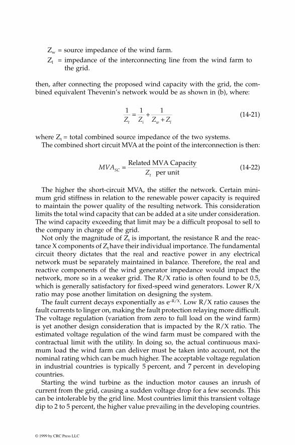
© 1999 by CRC Press LLC
Zw = source impedance of the wind farm.Zl = impedance of the interconnecting line from the wind farm to
the grid.
then, after connecting the proposed wind capacity with the grid, the com-bined equivalent Thevenin’s network would be as shown in (b), where:
(14-21)
where Zt = total combined source impedance of the two systems.The combined short circuit MVA at the point of the interconnection is then:
(14-22)
The higher the short-circuit MVA, the stiffer the network. Certain mini-mum grid stiffness in relation to the renewable power capacity is requiredto maintain the power quality of the resulting network. This considerationlimits the total wind capacity that can be added at a site under consideration.The wind capacity exceeding that limit may be a difficult proposal to sell tothe company in charge of the grid.
Not only the magnitude of Zt is important, the resistance R and the reac-tance X components of Zt have their individual importance. The fundamentalcircuit theory dictates that the real and reactive power in any electricalnetwork must be separately maintained in balance. Therefore, the real andreactive components of the wind generator impedance would impact thenetwork, more so in a weaker grid. The R/X ratio is often found to be 0.5,which is generally satisfactory for fixed-speed wind generators. Lower R/Xratio may pose another limitation on designing the system.
The fault current decays exponentially as e–R/X. Low R/X ratio causes thefault currents to linger on, making the fault protection relaying more difficult.The voltage regulation (variation from zero to full load on the wind farm)is yet another design consideration that is impacted by the R/X ratio. Theestimated voltage regulation of the wind farm must be compared with thecontractual limit with the utility. In doing so, the actual continuous maxi-mum load the wind farm can deliver must be taken into account, not thenominal rating which can be much higher. The acceptable voltage regulationin industrial countries is typically 5 percent, and 7 percent in developingcountries.
Starting the wind turbine as the induction motor causes an inrush ofcurrent from the grid, causing a sudden voltage drop for a few seconds. Thiscan be intolerable by the grid line. Most countries limit this transient voltagedip to 2 to 5 percent, the higher value prevailing in the developing countries.
1 1 1Z Z Z Zt i w l
= ++
MVAZSC
t
=Related MVA Capacity
per unit

© 1999 by CRC Press LLC
Fortunately, for wind farms with many machines, the machines can bestarted in sequence to minimize this effect. For very weak system, however,this issue can limit the number of machines that can be connected with thegrid lines. The voltage flicker severity increases as the square root of thenumber of machines. The flicker caused by starting one machine variesinversely with the fault level at the point of the grid connection, hence canbe an issue on the weaker grids.
Harmonics are generated by the power electronics employed for the softstart of large wind turbines and for the speed control during energy produc-ing operation. The former can be generally ignored due to the short durationand use of the sequential starts.
The operating harmonics, however, need to be filtered out. Total harmoniccontent of the wind farm is empirically found to depend on the square rootof the number of machines. Since the high voltage grid side has lowercurrent, designing the pulse-width-modulated (PWM) converters on the gridside can be advantageous. The utility companies around the world are notconsistent in the way they limit the harmonics. Some limit the harmonics interms of the absolute current in amperes, while others set limits proportionalto the grid’s short-circuit MVA at the point of interconnection.
Utilities find it convenient to meet the power-quality requirements bylimiting the total renewable power rating less than a few percent of the short-circuit MVA of the grid at the proposed interface. The limit is generally2 percent in developed countries and 5 percent in developing countries. Thisrequirement can be more restrictive than the overall power quality require-ment imposed in accordance with the national standards.
14.8.2 Interfacing Standards
The maximum capacity the renewable power plant can install is primarilydetermined from the electrical system and power quality considerationspresented in this chapter. A rough rule of thumb to control the power qualityhas been to keep the renewable power plant capacity in MW less than thegrid line voltage in kV if the grid is stiff (large). On a weak grid, however,only 10 or 20 percent of this capacity may be allowed. The regulation gen-erally imposed on the renewable power farms these days are in terms of theshort-circuit capacity at the proposed interface site.
We recall that the major power quality issues discussed in this chapter areas follows:
• the acceptable voltage range on the distribution system.• the step load voltage.• the steady state voltage regulations.• flickers caused by the wind fluctuations.• the harmonics.

© 1999 by CRC Press LLC
The acceptable voltage variations in the grid voltage at the distributionpoint in four countries are given in Table 14-2. The limit on the step-changea customer can cause on loading or unloading is listed in Table 14-3. It iscomplex to determine the maximum renewable capacity that can be allowedat a given site which will meet all these complex requirements. It may beeven more difficult to demonstrate the compliance. Under the situation, somecountries impose limits in percent of the grid short-circuit capacity. Forexample, such limits in Germany and Spain are listed in Table 14-4, butsimilar limits are evolving in other countries.
The power quality standards applicable specifically to grid-connectedwind farms are being drafted by the International Electrotechnical Commis-sion. It is expected that such standards would be more realistic than the rigidcriteria based on the ratio of the wind turbine capacity to the short-circuitMVA of the grid. The ultimate results would be consistent and predictable
TABLE 14-2
Acceptable Voltage Variation at Distribution Points (Low Voltage Consumers May See Wider Variations)
Country Acceptable range
U.S.A. ±5 percentFrance ±5 percentU.K. ±6 percentSpain ±7 percent
TABLE 14-3
Allowable Step-Change in Voltages a Customer can Cause by Step Loading or Unloading
Country Allowable range
France ±5 percentU.K. ±3 percentGermany ±2 percentSpain ±2 percent for wind generators
±5 percent for embedded generators
TABLE 14-4
Renewable Power Generation Limit in Percent of the Grid Short Circuit Capacity at the Point of Interface
Country Allowable limit
Germany 2 percentSpain 5 percentOther countries Evolving

© 1999 by CRC Press LLC
understanding on the power quality requirements and less cost-related indesigning wind farms to comply with the power quality issues.
Again, in order to control the quality of power, a rough rule of thumb hasbeen to keep the renewable power plant capacity in MW less than the gridline voltage in kV if the grid is stiff (large). On a weak grid, however, only10 or 20 percent of this capacity may be allowed.
14.9 Lightning Protection
The risk of mechanical and thermal damage to the blades and the electricalsystems due to lightning is minimized by a coordinated protection schemeusing lightning arresters and spark gaps6-7 in accordance with the Interna-tional Standards. The IEC Standard -1024-1 covers the requirements forprotection of structures against lightning. The electrical generator and trans-formers are designed with certain minimum Basic Insulation Level (BIL)consistent with the lightning risk in the area. The risk is proportional to thenumber of thunderstorms per year in the area. Figure 14-12 depicts thenumber of thunderstorms per year in the United States and southern Canada.
Tall towers are more vulnerable to the lightning risk. Among the valuablenew experience in the wind power industry is that the offshore wind powertowers experience a higher than average incidence of lightning strikes. Basedon such experience, the system manufacturer has addressed the design prob-lems. Figure 14-13 is one such solution developed by Vestas Wind Systemsof Denmark. The lightning current is dispersed to the ground though a seriesof spark gaps and equipotential bonding at joints. The transformer is pro-tected by placing it inside the tower.
FIGURE 4-12Thunderstorm frequency in the United States and Southern Canada. The contour lines indicatethe average number of days per year with thunderstorm occurrence.
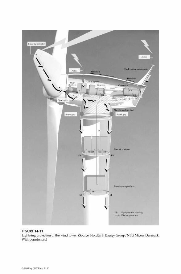
© 1999 by CRC Press LLC
FIGURE 14-13Lightning protection of the wind tower. (Source: Nordtank Energy Group/NEG Micon, Denmark.With permission.)

© 1999 by CRC Press LLC
14.10 National Electrical Code® on Renewable Power Systems
The 1996 revision of the National Electrical Code8 has established electricalsystem requirements on the wind and photovoltaic power systems. Thephotovoltaics are covered in Article 690. The Article 705 covers all renewableand cogeneration power systems, including the wind, which is reproducedin Appendix 1 of this book.
References
1. Adkins, B. 1964. “The General Theory of Electrical Machines,” London, Chap-man and Hall, 1964.
2. Kron, G. 1967. “Equivalent Circuits of Electrical Machines,” New York, DoverPublications, 1967.
3. Oliva, A. R., Balda, J. C., McNabb, D. W., and Richardson, R. D. 1997. “Powerquality monitoring of a pv generator,” IEEE paper No. PE-507-EC0-07, 1997.
4. Feijoo, A and Cidras, J. 1997. “Analyses of mechanical power fluctuations inasynchronous WECs,” IEEE paper No. PE-030-EC-0-1 0, 1997.
5. Gardner, P. 1997. “Wind farms and weak networks,” Wind Directions, Magazineof the European Wind Energy Association, London, July 1997.
6. Risø National Laboratory. 1996. “Power quality and grid connection of windturbines” — Summary report R-853, Denmark, October 1996.
7. Lewis, W. W. 1965. “The Protection of Transmission Systems Against Light-ning,” New York, Dover Publications, 1965.
8. National Fire Protection Association. 1996. National Electrical Code Handbook,7th Ed., Quincy, MA, 1996.

© 1999 by CRC Press LLC
15
Plant Economy
The economic viability of a proposed plant is influenced by several factorsthat contribute to the expected profitability. Since the profitability inadvert-ently varies with variations in the contributing factors, the sensitivity of theexpected profitability is analyzed with variances around their expected val-ues. The sensitivity analysis raises the confidence level of potential investors.This is important for both the wind and pv systems, but more so for windsystems whose profitability is extremely sensitive to the wind speed variations.
The primary factors contributing to the economic viability of the plantsare discussed in this chapter. The results are displayed in easy-to-use chartsfor screening the profitability of a proposed plant.
15.1 Energy Delivery Factor
The key economic performance measure of a power plant is the electricalenergy it delivers over the year. Not all power produced is delivered to thepaying customers. A fraction of it is used internally to power the controlequipment, meeting the power equipment losses and for the housekeepingfunctions such as lighting. In a typical wind farm or pv park, about 90 percentof the power produced is delivered to the customers, and the remaining isself-consumed for the plant operation.
The quantity of energy delivered depends on the peak power capacity ofthe site and how fully that capacity is utilized over every hour of the year.The normalized measure of the power plant performance is the EnergyDelivery Factor (EDF). It is defined as the ratio of the electrical energydelivered to the customers to the energy that can be delivered by the plantif it could be operated at the fully installed capacity during all 8,760 hoursof the year, that is as follows:
(15-1)Average annual EDFkWh delivered over the year
Installed capacity Number of hours in the year=
⋅

© 1999 by CRC Press LLC
Since the load power varies over the time, the EDF takes the integral form:
(15-2)
where P
m
= Plant capacity (the maximum power the plant can deliver)P
o
= Power delivered to the customers at any time t
The EDF is usually determined by bookkeeping the sum of the energydelivered over a continuous series of small discrete time intervals, that is asfollows:
15-3)
where P
avg
= average power delivered over the small time interval
∆
t.The EDF is a figure of merit that measures how hard the plant is utilized to
deliver the maximum possible energy. Not only does it include the energyconversion efficiencies of various components, it also accounts for the reliabil-ity, maintainability, and availability of the overall plant over the entire year.
The EDF is useful in comparing the economic utilization of one site overthe other, or the annual performance of a given site. Wind plants operatewith the annual average EDF around 30 percent, with some plants reportingEDF as high as 40 percent. This compares with 40 to 80 percent for theconventional plants. The base load plants operate at the higher end of therange.
The wind farm energy delivery factor varies with season and that mustbe taken into account. For example, the quarterly average EDF in Englandand Wales from the beginning of 1992 to the end of 1996 are shown inFigure 15-1. The operating data show rather wide variations, ranging from15 to 45 percent. The EDF is high in the first quarter and low in the lastquarter of every year. Even with the same kWh produced per year, theaverage price per kWh the plant may fetch could be lower if the seasonalvariations are wide.
15.2 Initial Capital Cost
The capital cost depends on the size, site and the technology of the plant.Typical ranges for various types of large power plants are given in Table 15-1.
Average annual EDF =⋅
⋅
∫ P dt
P
o
year
m 8760
Average annual EDF =⋅( )
⋅
∑P t
P
avg
year
m
∆
8760

© 1999 by CRC Press LLC
The costs of technologically matured coal and gas turbine plants are risingwith inflation, whereas the wind and pv plant costs are falling with newdevelopments coming in the market. Therefore, the renewable power plantcost must be estimated with their component costs current at the time ofprocurement, which may be lower than those at the time of planning.
The percent breakdown of the component costs in the total initial capitalcost of a typical wind farm is shown in Table 15-2. The single largest costitem is the turbine blades and rotor assembly, as expected.
15.3 Availability and Maintenance
The failure rates and effects determine the maintenance cost and availabilityof the plant to produce power. The past data on the operating experience is
FIGURE 15-1
Capacity factors of operating wind farms in England and Wales. (Source: U.K. Department ofTrade and Industry, Renewable Energy Technology Status Report, August 1997. With permission.)
TABLE 15-1
Capital Cost for Various Power Technologies
Plant Technology Capital Cost, $/kW
Wind Turbines 500–800Solar Photovoltaics 2000–4000Solar thermal(Solar II type)
3000–5000(land ~15 acres/MW)
Coal Thermal (Steam-Turbine) 400–600(land ~ 10 acres/MW)
Combined Cycle Gas-Turbine 800–1200
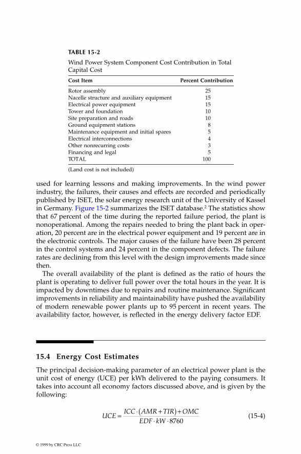
© 1999 by CRC Press LLC
used for learning lessons and making improvements. In the wind powerindustry, the failures, their causes and effects are recorded and periodicallypublished by ISET, the solar energy research unit of the University of Kasselin Germany. Figure 15-2 summarizes the ISET database.
2
The statistics showthat 67 percent of the time during the reported failure period, the plant isnonoperational. Among the repairs needed to bring the plant back in oper-ation, 20 percent are in the electrical power equipment and 19 percent are inthe electronic controls. The major causes of the failure have been 28 percentin the control systems and 24 percent in the component defects. The failurerates are declining from this level with the design improvements made sincethen.
The overall availability of the plant is defined as the ratio of hours theplant is operating to deliver full power over the total hours in the year. It isimpacted by downtimes due to repairs and routine maintenance. Significantimprovements in reliability and maintainability have pushed the availabilityof modern renewable power plants up to 95 percent in recent years. Theavailability factor, however, is reflected in the energy delivery factor EDF.
15.4 Energy Cost Estimates
The principal decision-making parameter of an electrical power plant is theunit cost of energy (UCE) per kWh delivered to the paying consumers. Ittakes into account all economy factors discussed above, and is given by thefollowing:
(15-4)
TABLE 15-2
Wind Power System Component Cost Contribution in Total
Capital Cost
Cost Item Percent Contribution
Rotor assembly 25Nacelle structure and auxiliary equipment 15Electrical power equipment 15Tower and foundation 10Site preparation and roads 10Ground equipment stations 8Maintenance equipment and initial spares 5Electrical interconnections 4Other nonrecurring costs 3Financing and legal 5TOTAL 100
(Land cost is not included)
UCEICC AMR TIR OMC
EDF kW= ⋅ +( ) +
⋅ ⋅8760

© 1999 by CRC Press LLC
where ICC = Initial capital cost, including land cost and startup cost up tothe time the first unit of energy is sold
AMR = Amortization rate per year as a fraction of the ICC
FIGURE 15-2
Wind power plant failure, cause, effect, and repair statistics. (Source: Institute of Solar Energyand Technology, University of Kassel, Germany, With permission.)

© 1999 by CRC Press LLC
TIR = Tax and insurance rate per year as a fraction of the ICCOMC = Operating and maintenance cost per yearEDF = Energy delivery factor over one year, as defined earlierkW = Kilowatt electrical power capacity installed
The amortization rate AMR reflects the cost of money, generally taken as0.10 to 0.20 depending on the prevailing mortgage interest rates availablefor such a project. The energy delivery factor EDF accounts for the variationsin the impinging energy (sun intensity or wind speed) at the proposed site,and all downtimes, full or partial. It is also a strong function of the reliabilityand maintainability of the plant over the entire year.
The present costs of various energy sources are summarized in Table 15-3.It shows that the wind power now compares well with the conventional coalthermal power.
15.5 Sensitivity Analysis
Accurately estimating the cost of electricity produced is not sufficient. Theproject planners must also carry out the sensitivity analysis, in that theenergy cost is estimated with a series of input parameters deviating on bothsides of the expected values. The sensitivity of the energy cost on the fol-lowing two factors is discussed in this section:
• variation in the wind speed.• variation in solar irradiation.
15.5.1 Effect of Wind Speed Variations
Since the energy output of the wind plant varies with the cube of the windspeed, a several percent change in the speed can have significant impact on
TABLE 15-3
Energy Generation Cost with Various
Power Technologies
Plant Technology
Generation Cost(Fuel + Capital)U.S. cents/kWh
Wind Turbines 5–7Solar Photovoltaics 15–25Solar thermal (Solar II type) 8–10Coal Thermal (Steam-Turbine) 3–4Combined Cycle Gas-Turbine 5–7
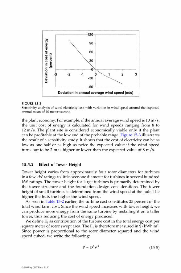
© 1999 by CRC Press LLC
the plant economy. For example, if the annual average wind speed is 10 m/s,the unit cost of energy is calculated for wind speeds ranging from 8 to12 m/s. The plant site is considered economically viable only if the plantcan be profitable at the low end of the probable range. Figure 15-3 illustratesthe result of a sensitivity study. It shows that the cost of electricity can be aslow as one-half or as high as twice the expected value if the wind speedturns out to be 2 m/s higher or lower than the expected value of 8 m/s.
15.5.2 Effect of Tower Height
Tower height varies from approximately four rotor diameters for turbinesin a few kW ratings to little over one diameter for turbines in several hundredkW ratings. The tower height for large turbines is primarily determined bythe tower structure and the foundation design considerations. The towerheight of small turbines is determined from the wind speed at the hub. Thehigher the hub, the higher the wind speed.
As seen in Table 15-2 earlier, the turbine cost constitutes 25 percent of thetotal wind farm cost. Since the wind speed increases with tower height, wecan produce more energy from the same turbine by installing it on a tallertower, thus reducing the cost of energy produced.
We define E
1
as contribution of the turbine cost in the total energy cost persquare meter of rotor swept area. The E
1
is therefore measured in $/kWh·m
2
.Since power is proportional to the rotor diameter squared and the windspeed cubed, we write the following:
(15-5)
FIGURE 15-3
Sensitivity analysis of wind electricity cost with variation in wind speed around the expectedannual mean of 10 meter/second.
P D V∝ 2 3

© 1999 by CRC Press LLC
The energy captured over the life of the turbine is also proportional to thesame parameters, i.e., D
2
and V
3
. In a matured competitive market, the rotorcost would be proportional to the swept area, hence D
2
, although it is farfrom that stage in the current rapidly evolving market. However, assumingthe competitive market E
1
is as follows:
(15-6)
As seen earlier in Equation 4-34, the wind speed varies with tower heightin the exponential relation:
(15-7)
where H = tower height at the hub.Combining Equations 15-6 and 15-7, we obtain:
(15-8)
The parameter
α
varies with the terrain type. Table 4-3 in Chapter 4 givesthis parameter value of 0.10 over the ocean, 0.40 over urban areas with tallbuildings and the often used average of 0.15 (~1/7) in areas with foot highgrass on flat ground. Even higher value of 0.43 was estimated for a NewEngland site at Stratton, Mt. Vermont.
1
With such variations in
α
, the windspeed can vary with H over a wide range from H
0.3
to H
1.3
.Equation 15-8 clearly indicates that the turbine contribution in cost of
energy per unit swept area decreases at least with the square root of thetower height. With the average value of
α
of 1/7, the turbine cost contribu-tion is approximately:
(15-9)
In rough terrain, the tower height can be extremely beneficial as shownby the following equation with
α
= 0.4:
(15-10)
Equations 15-9 and 15-10 indicate that there is not much benefit in increas-ing the tower height of the offshore installations. However, on rough terrain,increasing the tower height from 30 to 60 meters would decrease the contri-bution of the turbine cost per kWh/m
2
by 56 percent, a significant reduction.
E D D V V12 2 3 31∝ ∝
V H∝ α
EH1 3
1∝ α
Turbine cost per kWh per m EConstant
Tower Height2 , 1 =
Turbine cost per kWh per m EConstant
H2
1.2, 1 =

© 1999 by CRC Press LLC
Therefore, determining the
α
parameter accurately for the specific site isimportant in the estimate of the plant economy. An uneconomical site usinga short tower or conservative estimate of
α
can turn out to be profitable witha tall tower or the site specific estimate of
α
.
15.6 Profitability Index
As with the conventional projects, the profitability is measured by the prof-itability index, defined as the following:
(15-11)
By definition, the PI of zero gives the break-even point.The profitability obviously depends on the price at which the plant can
sell the energy it produces. In turn, it depends on the prevailing market pricethe utilities are charging to the area customers. Regions with high energycost could be more profitable if the capital cost isn’t high in the same pro-portion. Table 15-4 lists the 1997 average electricity prices in certain regionsof the U.S.A. The average price in the United Kingdom is about 8 pence/kWh(about 13 cents/kWh).
Inputs to the renewable power plant profitability analysis include thefollowing:
• anticipated energy impinging the site, that is the wind speed athub height for the wind farm or the insolation rate for the pv park.
• expected initial capital cost of installing the farm.• cost of capital, usually the interest rate on the loans.
TABLE 15-4
Average Electricity Prices for U.S. Residential
Customers in High Cost Areas in 1997
Utility area Cents/kWh
Long Island Lighting, New York 17Consolidated Edison, New York 16Public Service of New Hampshire 15New York State Electric and Gas 14Commonwealth Energy Systems, MA 14Central main Power (Main) 13PECO Energy, Philadelphia, PA 13Public Service Electric (New Jersey) 13
(Average price in the U.K.
≈
8 pence/kWh
≈
13 cents/kWh)
PI = Present worth of future revenues — Initial project costInitial project cost

© 1999 by CRC Press LLC
• expected economic life of the plant.• operating and maintenance cost.• average selling price of the energy generated from the farm.
A detailed multivariable profitability analysis with the above parametersis always required before making financial investments. Potential investorscan make initial profitability assessment using screening charts. The follow-ing sections present easy-to-use profitability charts for initial screening ofthe wind and pv power plant sites.
15.6.1 Wind Farm Screening Chart
Figure 15-4 is a wind farm profitability screening chart based on cost of capital(discount rate) of 8 percent, project life of 15 years, initial cost of 1,100 Euro-pean currency units per kW capacity, and the operating and maintenance costof 3 percent of the initial project cost.
3
The chart takes into account the inflationat a constant rate, i.e., the costs and revenues rising at the same rate. Thetaxes on sales, if any, must be deducted from the average selling price beforeit is entered in reading the chart. An example for using the chart follows:
At a site with 7.5 m/s wind speed at hub height, the profitability index wouldbe zero (a break-even point) if the energy can be sold at 0.069 ECU/kWh. Ifthe energy price is 0.085 ECU/kWh, the profitability index would be 0.30,generally an attractive value for private investors. At a site with only 7 m/swind speed, the same profitability can be achieved if the energy can be soldat 0.097 ECU/kWh.
15.6.2 pv Park Screening Chart
Similar screening charts for pv stand-alone or grid-connected systems areshown in Figures 15-6 and 15-7.
4
For these charts, the yearly energy deliveryE
y
in kWh/year is defined as the following:
(15-12)
where K
p
= performance ratio of the systemH
y
= yearly solar irradiation in the plane of the modules, kWh/m
2
/yearP
pk
= installed peak power under the standard test conditions of1 kW/m
2
solar irradiation, the cell junction operating tempera-ture of 25°C and the air mass of 1.5.
The pv energy conversion efficiency of the modules is included in P
pk.
Thetypical values of K
p
for well designed systems are 0.7 to 0.8 for gird-connected
E K H P kWh yeary p y pk= ⋅ ⋅

© 1999 by CRC Press LLC
systems without batteries and delivering AC power using inverters, and0.5 to 0.6 for stand-alone systems using batteries and delivering DC power.
The input to the figures are the initial capital cost of the pv system indollars per peak watt capacity I
up
, the cost of capital, the life of the plant,the operating and maintenance cost K
om
, the yearly solar irradiation H
y
, andthe performance parameter K
p
as defined above. With these inputs, the chartgives the overall discounted cost (ODC) of electricity delivered. The life ofthe plant in years, n, can be the desired payback period to recover the initialinvestment, or the full economic life of the plant. In the latter case, the ODCis known as the life cycle cost (LCC) of the energy delivered. The chart isprepared with typical values for large pv farms, such as K
p
of 0.75, 8 percentcost of capital, 20 years life and 2 percent operating and maintenance cost.
FIGURE 15-4
Profitability chart for wind farms. (Source: B. Chabot – ADME, France, and Wind Directions,Magazine of the European Wind Energy Association, London, October 1997. With permission.)

© 1999 by CRC Press LLC
An example of using Figure 15-5 follows. At a solar site with H
y
of2,000 kWh/m
2
/yr and the capital cost of 5 $/Wp, we see that the energycost would be $0.40 per kWh delivered. For the cost of energy delivered tobe below 0.20 $/kWh, the capital cost of the plant must be $2.50 per Wp.With new pv technologies being developed and made commercially avail-able at lower costs, the capital cost below 3 $/W
p
is realizable.Being costlier than the wind power systems, the pv systems at present are
more likely to be installed in remote areas where higher cost can be justifiedand partially offset by low interest loans. Figure 15-6 is cast in terms of theprofitability index defined earlier. The parameters for this chart are thecapital cost of 4 $/W
p
, 3 percent cost of capital, 30 years economic life,1 percent operating and maintenance cost and the performance parameter
FIGURE 15-5
Overall discounted cost of pv energy. (Source: B. Chabot – ADME, France and Progress inPhotovoltaic Research and Applications, Volume 6, p. 58, 1998. John Wiley & Sons Limited,Bristol, U.K.. With permission.)
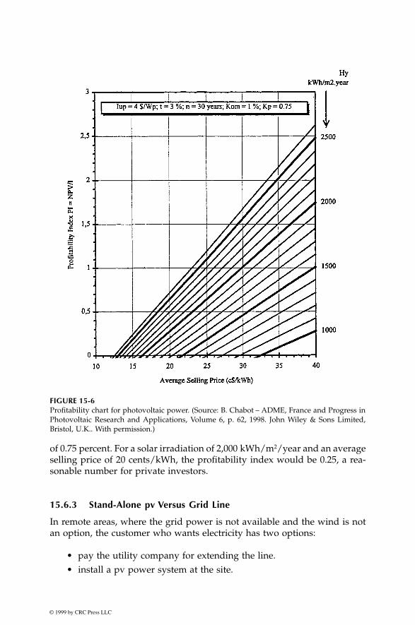
© 1999 by CRC Press LLC
of 0.75 percent. For a solar irradiation of 2,000 kWh/m
2
/year and an averageselling price of 20 cents/kWh, the profitability index would be 0.25, a rea-sonable number for private investors.
15.6.3 Stand-Alone pv Versus Grid Line
In remote areas, where the grid power is not available and the wind is notan option, the customer who wants electricity has two options:
• pay the utility company for extending the line.• install a pv power system at the site.
FIGURE 15-6
Profitability chart for photovoltaic power. (Source: B. Chabot – ADME, France and Progress inPhotovoltaic Research and Applications, Volume 6, p. 62, 1998. John Wiley & Sons Limited,Bristol, U.K.. With permission.)

© 1999 by CRC Press LLC
The cost of extending the line may be prohibitive if the stretch is long. Fora given distance of the line extension, the line cost is fixed. The economy ofthe electrical energy, therefore, clearly depends on the energy demand inkWh per day. Figure 15-7 is a screening chart for making economic choicebetween the line extension and a pv plant at site. It is developed using the1997 average utility charges for line extension and pv modules price. As anexample of using the chart, if the customer needs 10 kWh/day and livesthree miles away from the nearest power line, the stand-alone pv at the sitewould be economical. If the distance were one mile instead, the line extensionwould be economical. The break-even distance for this customer is about1.7 miles. For another customer who needs 20 kWh/day, the break-evendistance is three miles.
In getting the line extension, rural utilities and their customers face con-flicting interest. The utility is interested in controlling the cost, and thecustomer is interested in reliable power. In selected low population densityareas of the U.S.A., some utility companies offer their customers a choice ofinstalling a pv system as an alternative to costly emergency service and longstretches of the line dedicated to serve one or a few customers.
This is how some U.S. utility companies in rural areas are responding topotential pv customers:
• customer interested in electric power contacts the utility company.• determination is made whether the point-of-service will be eco-
nomically served by extending a line or by installing a pv systemat the site.
• utility company develops the pv design.• the system is installed by an independent contractor.
FIGURE 15-7
Stand-alone pv plant or line extension costs for various levels of energy need based on average1997 costs of Idaho Power Company.

© 1999 by CRC Press LLC
• the total capital cost is paid by the utility company.• the utility company is responsible for maintenance of the system.• customer is billed a fixed monthly rate, rather than the amount
based on the energy consumed.
This approach spreads out the burden of the initial capital cost on thecustomer.
15.7 Hybrid Economics
A detailed analytical tool to evaluate the economics of hybrid systems hasbeen developed by the National Renewable Energy Laboratory. The newerversion, Hybrid2
5
allows the user to determine basic economic figures for aparticular simulation run. The economics module uses information from theperformance simulation run and economic data supplied by the user. Itcomputes parameters as the payback period, internal rate of return, cashflow, and equipment replacement expenses. The user has a wide versatilityin determining the expense of the project and what inputs to include. Param-eters such as grid extension, importation tariffs, systems administrationcosts, and taxes can be included in the analysis. The user may conductcomparisons between differing hybrid possibilities and power solutions, anddetermine approximate costs. Figure 15-8 is the computer screen displayingthe choices available to the user. As indicated by the menu buttons, itincludes wind, pv, diesel, and battery.
Hybrid2 allows user to conduct parametric analyses on certain cost param-eters, such as fuel cost, discount rate, and inflation rate to help determinehow the value of certain parameters can affect the viability of the project.
As for the project funding, there have been strong financial incentives forthe renewable power in many countries around the world. However, theincentives have been declining because the renewables are becoming eco-nomically competitive on their own merits. More projects are being fundedstrictly on the commercial basis. Enviro Tech Investment Funds in the U.S.A.is a venture-capital fund supported by Edison Electric Institute (an associa-tion of investor-owned electric utility companies providing 75 percent of thenation’s electricity). The World Bank now includes the wind and pv in itslanding portfolios. The first such loan was made to India in 1993. Severalunits in the World Bank group are jointly developing stand-alone projectsin developing countries.

© 1999 by CRC Press LLC
References
1. Cardell, J. B. and Connors, S. R. 1997. “Wind power in New England, modelingand analyses of nondispatchable renewable energy technologies,”
IEEE PaperNo. Power Engineering-888-PWRS-2-06,
1997.2. Institute of Solar Energy and Technology. 1997. “Annual Report,” Germany,
University of Kassel, 1997.3. Chabot, B. 1997. “L’analyse economique de l’energie ecolienne,”
Revue de l’En-ergie,
ADME, France, No. 485, Feb. 1997.4. Chabot, B. 1998. “From Costs to Prices: economic analyses of photovoltaic
energy and services,”
Progress in Photovoltaic Research and Applications,
Vol. 6,p. 55-68, 1998.
5. Baring-Gould, E. I. 1996. “Hybrid2, The hybrid system simulation model usermanual,”
NREL Report No. TP-440-21272,
June 1996.
FIGURE 15-8
Hybrid2 economic simulation model. (Source: Ian Baring-Gould, National Renewable EnergyLaboratory, Golden, Colorado. With permission.)

© 1999 by CRC Press LLC
16
The Future
The presented trends and future forecasts of the electricity demand, and howphotovoltaic and wind power may grow in percentage of the total demandare discussed in this chapter. The historical data on the market developmentsin similar basic-need industries and the Fisher-Pry market growth modelindicate that the pv and wind power may reach their full potential in theyear 2065. The probable impact of the U.S. utility restructuring on the renew-ables is reviewed.
16.1 World Electricity Demand to 2015
According to the U.S. Department of Energy, electric power is expected to bethe fastest growing source of energy to the end users throughout the worldover the next two decades. The electricity demand is projected to grow to 19trillion kWh by the year 2015 (Figure 16-1) at the annual growth rate of2.6 percent.
1
The electricity demand in the industrial and developing coun-tries projected to 2015 is shown in Figure 16-2, indicating a fast growth ratein the developing countries. Table 16-1 shows the per capita consumption byregion and country. The Organization for Economic Cooperation and Devel-opment (OECD) countries constitutes 20 percent of the world’s population,but consumes over 60 percent of the world’s electricity. The non-OECD Asiais expected to grow faster than the Eastern European and Former SovietUnion (EE/FSU) countries. This is a result of the relatively high economicgrowth rate projected for the non-OECD Asia. Although the United States isthe largest consumer of electricity in the world, it has the lowest projectedgrowth rate of 1.3 percent versus the world average of 2.6 percent. Mexicohas the highest projected growth rate of 4.7 percent per year to the year 2015.
The developing Asia is projected to experience the strongest growth thanany other region in the world at a growth rate of 5 percent per year(Figure 16-3). As the electricity demand grows, the coal will remain theprimary fuel for power generation, especially in China and India. The shareof nuclear generation worldwide has reached the peak, and is expected todecline in the future. The coal, the natural gas, and the renewable, all are

© 1999 by CRC Press LLC
expected to grow to replace the retiring nuclear power plants. However, therenewables are expected to take a greater percentage of the growth. Forexample, in February 1997, the Swedish government announced that it
FIGURE 16-1
World electricity consumption 1970-2015. (Source: U.S. Department of Energy, InternationalEnergy Outlook 1997 with Projections to 2015, DOE Office of the Integrated Analysis andForecasting, Report No. DE-97005344, April 1997.)
FIGURE 16-2
Electricity consumption by industrialized and developing countries 1990-2015. (Source: U.S.Department of Energy, International Energy Outlook 1997 with Projections to 2015, DOE Officeof the Integrated Analysis and Forecasting, Report No. DE-97005344, April 1997.)
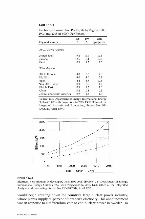
© 1999 by CRC Press LLC
would begin shutting down the country’s large nuclear power industry,whose plants supply 50 percent of Sweden’s electricity. This announcementwas in response to a referendum vote to end nuclear power in Sweden. To
TABLE 16-1
Electricity Consumption Per Capita by Region, 1980,
1993 and 2015 in MWh Per Person
Region/Country198
0199
32015
(projected)
OECD North America
United Sates 9.2 11.1 12.6Canada 12.6 15.4 19.2Mexico 0.9 1.2 2.5
Other Regions
OECD Europe 4.0 5.0 7.8EE/FSU 4.0 4.0 5.1Japan
4.4
6.3 10.3Non-OECD Asia 0.3 0.5 1.2Middle East 0.9 1.3 1.6Africa 0.4 0.4 0.5Central and South America 0.9 1.3 1.7
(Source: U.S. Department of Energy, International EnergyOutlook 1997 with Projections to 2015, DOE Office of theIntegrated Analysis and Forecasting, Report No. DE-97005344, April 1997.)
FIGURE 16-3
Electricity consumption in developing Asia 1990-2015. (Source: U.S. Department of Energy,International Energy Outlook 1997 with Projections to 2015, DOE Office of the IntegratedAnalysis and Forecasting, Report No. DE-97005344, April 1997.)

© 1999 by CRC Press LLC
compensate, the government is to step up intervention in energy market andforce a switch to greater use of nonfossil alternatives. Other industrial coun-tries have serious commitments to reduce pollution of the environment.According to the Environmental Protection Agency of the U.S.A., the electricpower industry is the nation’s largest polluter. It is responsible for emitting66 percent of SO
2
, 29 percent of NOx, 36 percent of manmade CO
2
, and21 percent of mercury. The 160 countries, gathered in Kyoto, Japan, inDecember 1997 under the U.N. Convention on Climate Change, agreed towork on reducing emissions of carbon dioxide and other greenhouse gasesas per the national and regional goals depicted in Figure 16-4. The U.S. haspromised a 7 percent cut by the year 2008-2012 measured against the baseyear of 1990. Because the U.S. economy would grow by then since 1990, thereal cut required would be over 30 percent from the current level of emission.This is a significant challenge and would certainly require an aggressivepolicy on the renewable energy sources.
The developing countries have additional reason for promoting wind andpv programs. With significant rural population, they would benefit from thedistributed power generation near the loads.
16.2 Wind Future
The U.S. Department of Energy reports that wind is experiencing the stron-gest growth among the renewable energy sources with the falling generation
FIGURE 16-4
Cutting emissions under Kyoto treaty. (Source: United Nations.)
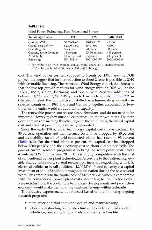
© 1999 by CRC Press LLC
cost. The wind power cost has dropped to 5 cents per kWh, and the DOEprojections suggest that further reduction to about 2 cents is possible by 2010with favorable financing. The American Wind Energy Association forecaststhat the five top-growth markets for wind energy through 2005 will be theU.S.A., India, China, Germany, and Spain, with capacity additions ofbetween 1,275 and 2,730 MW projected in each country. Table 2-2 inChapter 2 listed the cumulative installed wind-generating capacity inselected countries. In 1995, India and Germany together accounted for two-thirds of the entire world’s added wind capacity.
The renewable power sources are clean, abundant, and do not need to beimported. However, they must be economical on their own merit. The newdevelopments are meeting this challenge on the both fronts, the initial capitalcost and the cost per unit of electricity generated.
Since the early 1980s, wind technology capital costs have declined by80 percent, operation and maintenance costs have dropped by 80 percentand availability factor of grid-connected plants has risen to 95 percent(Table 16-2). For the wind plans at present, the capital cost has droppedbelow $800 per kW and the electricity cost to about 6 cents per kWh. Thegoal of current research programs is to bring the wind power cost below4 cents per kWh by the year 2000. This is highly competitive with the costof conventional power plant technologies. According to the National Renew-able Energy Laboratory, several research partners are negotiating with U.S.electrical utilities to install additional 4,200 MW of wind capacity at a capitalinvestment of about $2 billion throughout the nation during the next severalyears. This amounts to the capital cost of $476 per kW, which is comparablewith the conventional power plant costs. According to the Electric PowerResearch Institute, the continuing technology developments and productioneconomy would make the wind the least-cost energy within a decade.
The industry experts make this forecast based on the following ongoingresearch programs:
• more efficient airfoil and blade design and manufacturing.• better understanding on the structure and foundation loads under
turbulence, operating fatigue loads and their effect on life.
TABLE 16-2
Wind Power Technology, Past, Present and Future
Technology Status 1980 1997 After 2000
Cost per kWh* $0.35–$0.40 $0.05–$0.07 <$0.04Capital cost per kW $2,000–3,000 $500–800 <$500Operating life 5–7 years 20 years 30 yearsCapacity factor (average) 15 percent 25–30 percent >30 percentAvailability 50–65 percent 95 percent >95 percent Size range 50–150 kW 300–1000 kW 500–2,000 kW
* For wind sites with average annual wind speed of 7 meters/second(15.6 miles per hour) at 30 meters (100 feet) hub height.

© 1999 by CRC Press LLC
• computer prototyping by accurate system modeling and simulation.• integrated electrical generators and power electronics to eliminate
the mechanical gearbox.• efficient low cost energy storage at large scale.• better wind speed characterization, particularly within a large
wind farm.
Successful design, development, and demonstration based on the resultsof these research programs are expected to increase the share of wind powerin the U.S.A. from a fraction of 1 percent to more than 10 percent over thenext two decades.
The offshore wind potential is much greater than onshore due to goodwind speed and the large area available for commercial installations. It islimited only by practical working depths and other maritime activities inthe area of interest. Fishing, shipping routes, and military test grounds aresome of the activities that may conflict with the wind farm. Water depth of30 meters is practical. Taking only the water depth as a constraint, theaccessible U.K. offshore wind resource is estimated to be 380 TWh per year.Taking other constraints also into account, this estimate is reduced to 120 TWhper year.
A study commissioned by the European Union has suggested that theoffshore wind farms in the coastal regions of Germany, Holland, and Den-mark could meet all electricity demand in those countries. PowerGen Cor-poration of Britain plans to build 37 MW (25 towers, each rated 1.5 MW) ofoffshore wind capacity near Yarmouth, Norfolk, by 1999. Germany plans toinstall a large wind farm in the Baltic Sea, near Schleswig-Holstein.
Denmark’s ambitious offshore plan announced in the government’sEnergy-21 report published in 1997 aims to have at least 750 MW offshorecapacity by 2005, 2,300 MW by 2015 and 4,000 MW by the year 2030. Thiswill amount to about 50 percent of that country’s electricity coming fromwind. This would push the percentage limit to a practical maximum for anyintermittent source of power. The first group of Denmark’s offshore sites isshown in Figures 16-5 and 16-6.
The offshore wind speed is generally higher, typically 8 to 10 m/s. How-ever, due to lack of long term data, these estimates must account for theinherent variability in the estimate and the associated sensitivity to the costof generated electricity.
The onshore wind technology is applicable to the offshore installations.The major difference, however, is the hostile environment and the associatedincrease in the installation cost. The electrical loss in transmitting power tothe shore needs to be accounted for. Overall, it is estimated that the offshorewind power plant cost can be at least 30 percent higher than the comparableinland plant.

© 1999 by CRC Press LLC
As of December 1997, Europe’s wind capacity by country was shown inFigure 2-10. Germany and Denmark lead Europe in wind power. Both haveachieved phenomenal wind energy growth through a guaranteed tariff basedon the domestic electricity prices, perhaps a blueprint for the rest of theworld to follow. Germany has a 35-fold increase between 1990 and 1996, a70 percent annual rate of growth. With 2,000 MW installed, Germany is nowthe world leader. The former global leader, the U.S.A., has seen only a smallincrease during this period, from 1,500 MW in 1990 to 1,650 MW in 1996.
In 1997, the European Wind Energy Association adopted an ambitioustarget of 40,000 MW of wind capacity in Europe by the year 2010 and100,000 MW by 2020 (Table 16-3). Each European country would be obligatedto meet its committed share of renewable electricity, including the windenergy obligation, towards the overall target of 12 percent of the primaryenergy by wind in Europe by the year 2010.
In selected countries, the present wind capacity and future targets are listedin Table 16-4. The present and future targets for meeting the total electricitydemand by wind capacity are listed in Table 16-5. Based on these targets, itis reasonable to expect that the wind may contribute 10 to 25 percent of thetotal electricity demand in some countries by 2010.
FIGURE 16-5
Denmark’s first large offshore wind power sites. (Source: Wind Directions, Magazine of theEuropean Wind Energy Association, January 1998, London. With permission.)
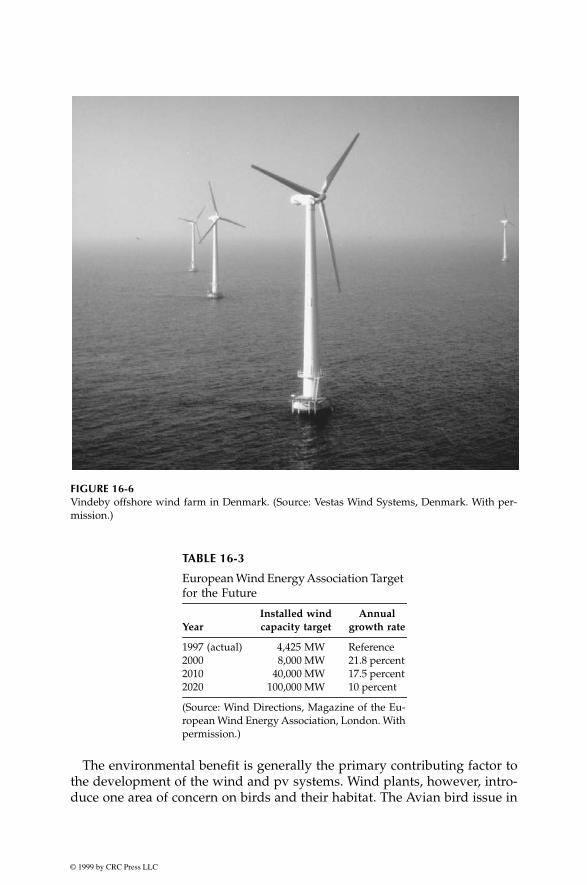
© 1999 by CRC Press LLC
The environmental benefit is generally the primary contributing factor tothe development of the wind and pv systems. Wind plants, however, intro-duce one area of concern on birds and their habitat. The Avian bird issue in
FIGURE 16-6
Vindeby offshore wind farm in Denmark. (Source: Vestas Wind Systems, Denmark. With per-mission.)
TABLE 16-3
European Wind Energy Association Target
for the Future
YearInstalled windcapacity target
Annual growth rate
1997 (actual) 4,425 MW Reference2000 8,000 MW 21.8 percent 2010 40,000 MW 17.5 percent2020 100,000 MW 10 percent
(Source: Wind Directions, Magazine of the Eu-ropean Wind Energy Association, London. Withpermission.)

© 1999 by CRC Press LLC
California is under research funded by the DOE and the wind industry todefine the magnitude of the problem and ways to prevent the bird kills. Thenoise factor and the impact on rural landscape are other concerns, whichmay impact the wind market development. These factors have begun tocontribute and make the planning process difficult in some countries. Thesheer speed at which new development has taken place has far outpacedthe capacities and capabilities of the decision makers. The regulations areinadequate to cover the installations of wind turbine in rural areas. The closerpeople watch the wind turbine rotating, and the smaller the local benefitsin terms of jobs and tax revenue becomes, the stronger the opposition. Somegovernments have started publishing clear guidelines in order to help localauthorities in the planning procedures.
TABLE 16-4
Present Wind Capacity and Future Targets in Selected Countries
Country Capacity
Germany 1,764 MW was operational as of June 1997Netherlands 2,750 MW target by 2020Denmark off-shore target 750 MW target by 2005
2,300 MW target by 20154,000 MW target by 2030
United Kingdom 160 MW was operational as of January 1996Ireland Government target 500 MW by 2010
IWEA target 1,000 MW by 2010 Italy 100 MW was operational as of November 1997USA 1,650 MW was operations as of December 1996
6,000 MW target by 200612,000 MW target by 2015
India 1,000 MW was operational as of December 1997
TABLE 16-5
Present and Future Target for Percent of Total
Electricity Demand Met by Wind Capacity
Country Wind as Percent of Total Electricity Demand
Denmark Was 6 percent as of June 1997Target 50 percent by 2030 (aggressive)
Germany Was 10 percent as of June 1997Target 20-25 percent by 2010
Ireland Government target 5 percent by 2010IWEA target 10 percent by 2010
USA Was <1 percent in 1997EPRI estimate 10 percent by 2020
(Source: Wind Directions, Magazine of the European WindEnergy Association, London, With permission.)
© 1999 by CRC Press LLC
16.3 pv Future
On the other hand, the cost of solar pv electricity is still high in the neigh-borhood of 15 to 20 cents per kWh. With the consumer cost of utility powerranging from 10 to 15 cents per kWh nationwide, pv cannot economicallycompete directly with the utility power as yet, except in remote marketswhere the utility power is not available and the transmission line cost wouldbe prohibitive. Many developing countries have large areas falling in thiscategory. With the ongoing research in pv technologies around the world,the pv energy cost is expected to fall to 12 to 15 cents per kWh or less in thenext several years as the learning curve and the economy of scale come intoplay. The research programs jointly funded by DOE and NREL have the goalof bringing down the pv electricity cost below 12 cents per kWh by the year2000.
The pv cell manufacturing process is energy intensive. Newer processesare being developed and continuously implemented to lower the energy useper square centimeter of the finished cell. In the current manufacturingprocess, the front and the back of the cells are diffused separately, takingone to three hours of manufacturing time. Researchers at the Georgia Insti-tute of Technology are considering rapid-thermal-processing technology.This process simultaneously forms the front and the back of the cell in severalminutes, and the metal contacts are applied by screen printing. It not onlycuts the processing time, it also lowers the temperature and energy neededfor fabrication.
Total worldwide production of pv modules has reached 100 MW, and isprojected to grow to almost 200 MW by 2000 (Figure 16-7). Approximately
of the current production in the U.S.A. is by two companies, SiemensSolar Industries in California and Solarex in Maryland.
Among the new advances underway in the pv technology, the thin film isexpected to lead the group. The amorphous silicon particularly holds themost near-term promise of quickly penetrating the market due to its lowmaterial and manufacturing costs. In this technology, 2 µm thick amorphoussilicon vapor is deposited on glass or stainless steel rolls, typically 2,000 feetlong and 13 inches wide. Compared to the thick crystalline silicon cells,amorphous silicon technology uses less than 1 percent material. The sheetmanufacturing, instead of single cells from ingots, offers a low-cost base.The disadvantage in single junction amorphous silicon is that the cell effi-ciency degrades about 20 percent in the first several months under the sun-light before stabilizing. At present, the stabilized efficiency is half and theretail price is also half, keeping the price per watt the same. However, thisis the market-based price, and not the technology-based price. The crystal-line-silicon technology has been with us for several decades and has entereda plateau of a slow learning curve. On the other hand, the amorphous-silicontechnology is new and, hence, the steep learning curve is expected. The
23⁄

© 1999 by CRC Press LLC
expected result is a rapid decline in the amorphous silicon price per watt byincreasing the efficiency and decreasing the manufacturing cost. On thispremise, two large amorphous-silicon-panel manufacturing plants startedin the U.S.A. in 1996. The technology and competition are expected to takehold on the market and the price, as they always have.
In the U.S.A., the pv and the wind power today are not competing on auniform playing field, as their costs do not fully reflect benefits of the fueldiversity and pollution free operation. For example, if the renewables getdue credits for pollution elimination of 600 tons of CO
2
per million kWhelectricity consumed, it would get a further boost in the incentives presentlyoffered by the United States Government. For the American pv and windindustries, there is an additional competition in the international market.Other governments support their companies with well-funded research, low-cost loans, and favorable tax rate tariffs not generally available to their U.S.counterparts.
16.4 Declining Production Costs
The economy of scale is expected to continue in contributing to the decliningprices. Future wind plants will undoubtedly be larger than those installedin the past, and the cost per square meter of the blade swept area decline
FIGURE 16-7
PV annual capacity and cumulative installed capacity worldwide. (Source: PV News, an indus-try publication.)

© 1999 by CRC Press LLC
with size. Figure 16-8 shows the prevailing costs of wind turbines of varioussizes in Germany. The price band is DM/m
2
of the blade area, falling from800 to 1200 DM/m
2
for small turbines to 500 to 800 DM/m2 for large turbinesof 50 meters diameter. The line showing the annual energy potential persquare meter rises from 630 kWh/m
2
in small turbines to 1,120 kWh/m
2
inlarge turbines of 46 meters diameter.
With the technology and the scale of economy combined, the manufactur-ing cost of new technologies has historically shown declining patterns. Thegrowth of new product eventually brings with it a stream of competitorsand the leaning curve benefits. A learning curve hypothesis has been com-monly used to model such cost declines. The cost is modeled as an expo-nentially decreasing function of the cumulative number of units producedup to that time. A standard form for a cost decline is constant doubling,where the cost is discounted by a fraction
λ
when the cumulative productiondoubles. For renewable electricity, the production units are MW of capacityproduced and kWh of electricity generated. If we want to monitor only oneproduction unit, the kWh generated includes both the MW capacity installedand the length of the operating experience, thus, making it an inclusive unitof production.
FIGURE 16-8
Economy of scale trends for capital cost in Deutsche mark/m2 and annual energy produced inkWh/m2 versus blade swept area. (Source: Institute of Solar Energy and Technology, Universityof Kassel, Germany. With permission.)
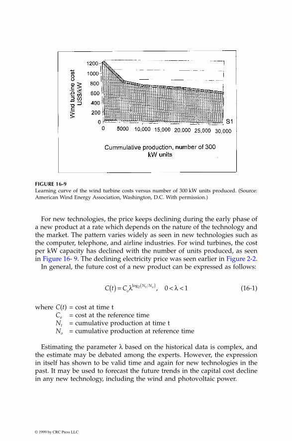
© 1999 by CRC Press LLC
For new technologies, the price keeps declining during the early phase ofa new product at a rate which depends on the nature of the technology andthe market. The pattern varies widely as seen in new technologies such asthe computer, telephone, and airline industries. For wind turbines, the costper kW capacity has declined with the number of units produced, as seenin Figure 16- 9. The declining electricity price was seen earlier in Figure 2-2.
In general, the future cost of a new product can be expressed as follows:
(16-1)
where
C
(
t
) = cost at time t
C
o
= cost at the reference time
N
t
= cumulative production at time t
N
o
= cumulative production at reference time
Estimating the parameter
λ
based on the historical data is complex, andthe estimate may be debated among the experts. However, the expressionin itself has shown to be valid time and again for new technologies in thepast. It may be used to forecast the future trends in the capital cost declinein any new technology, including the wind and photovoltaic power.
FIGURE 16-9
Learning curve of the wind turbine costs versus number of 300 kW units produced. (Source:American Wind Energy Association, Washington, D.C. With permission.)
C t CoN Nt o( ) = < <( )λ λlog , 2 0 1
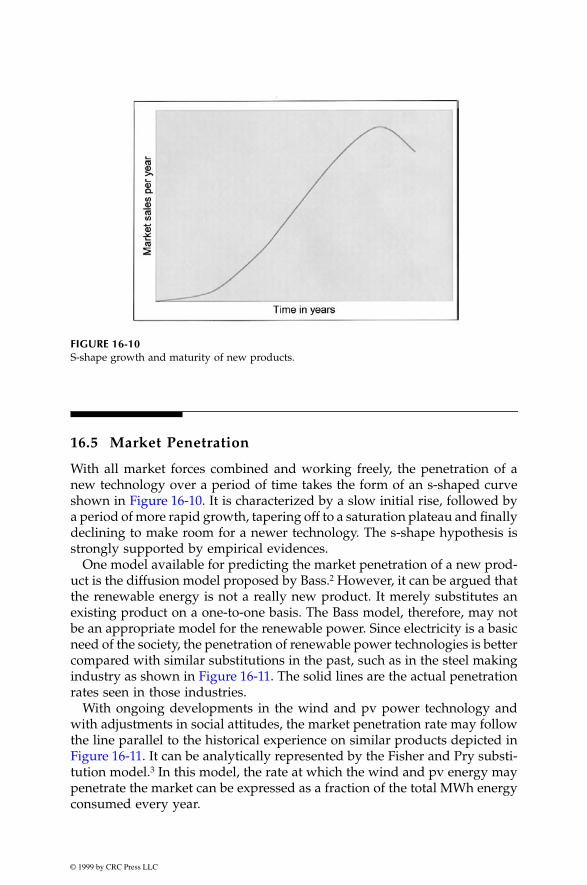
© 1999 by CRC Press LLC
16.5 Market Penetration
With all market forces combined and working freely, the penetration of anew technology over a period of time takes the form of an s-shaped curveshown in Figure 16-10. It is characterized by a slow initial rise, followed bya period of more rapid growth, tapering off to a saturation plateau and finallydeclining to make room for a newer technology. The s-shape hypothesis isstrongly supported by empirical evidences.
One model available for predicting the market penetration of a new prod-uct is the diffusion model proposed by Bass.
2
However, it can be argued thatthe renewable energy is not a really new product. It merely substitutes anexisting product on a one-to-one basis. The Bass model, therefore, may notbe an appropriate model for the renewable power. Since electricity is a basicneed of the society, the penetration of renewable power technologies is bettercompared with similar substitutions in the past, such as in the steel makingindustry as shown in Figure 16-11. The solid lines are the actual penetrationrates seen in those industries.
With ongoing developments in the wind and pv power technology andwith adjustments in social attitudes, the market penetration rate may followthe line parallel to the historical experience on similar products depicted inFigure 16-11. It can be analytically represented by the Fisher and Pry substi-tution model.
3
In this model, the rate at which the wind and pv energy maypenetrate the market can be expressed as a fraction of the total MWh energyconsumed every year.
FIGURE 16-10
S-shape growth and maturity of new products.

© 1999 by CRC Press LLC
If we let:
f = fraction of the market captured by the renewables at time t, andt
o
= time when f equals
then f can be expressed as follows:
(16-2)
FIGURE 16-11
Market penetration of new product substituting existing products. Wind and pv shown inparallel with historical data.
12⁄
fe
or
ff
e
b t t
b t t
o
o
=+
−=
− −( )[ ]
− −( )
1
1
1
,

© 1999 by CRC Press LLC
Here b is the growth constant, characterizing the growth to the potentialassociated with a particular technology. The equation gives log-linearstraight lines shown in Figure 16-11.
We take that the renewable power was successfully demonstrated to becommercially viable in the 1970s and made a commercial start in 1985. Thisis the time when a group of wind farms in California were installed andoperated for profit by private investors. Based on this premise and based onthe Fisher-Pry model just described, we draw the dotted line in Figure 16-11,beginning in 1985 and then running parallel to the historical lines followedby similar substitution products in the past. That is the rate of marketpenetration we can expect the wind and pv to follow in the future.
At the rate projected by the dotted line, the full 100 percent potential ofthe wind and pv will perhaps be realized around 2065. The wind and pvreaching the 100 percent potential in the year 2065 does not mean that theywill completely replace the thermal and other power. It merely means it willreach its fully attainable potential. Experts would argue on the upper limitof this potential for a given country. However, the wind and solar, beingintermittent sources of energy, cannot be the baseload provider. They mayaugment the baseload plants, thermal, or other types, which can dispatchenergy on demand. Such reasoning puts an upper limit on the pv and windpower to well below 50 percent, perhaps around 25 percent. According tothe Royal Institute of the International Affairs study published in the U.K.in May 1997, all renewable sources could provide between 25 to 50 percentof European electricity by the year 2030. The contributions of the wind andpv in the total electricity demand, however, will largely depend on theoperating experience with the grid-connected plants and energy storagetechnologies developed during the next few decades that can remedy thenondispatchable nature of the pv and wind energy. New energy storageproducts are being developed that incorporate batteries, flywheel, fuel cells,and superconducting coils into system solutions for the power industry suchas load leveling and power quality. Electric utility restructuring and thesubsequently increased competitive market are creating new and higher-value market for energy storage. The renewable power is the new marketopportunity for large-scale energy storage products.
The sophisticated prediction models have been developed by the DOE,NREL, and others based on mathematical considerations and regressionanalyses through applicable data. However, there is a limit to how suchmodels can be confidently used to commit huge sums of capital investments.Small errors in data can cause large errors in projections, particularly decadesout in the future. The time-proven data on how people make investmentdecisions under long-term uncertainties can also help. The experience indi-cates that investors commit funds only if the payback period is less than fiveyears, the shorter it is, the quicker the investment penetrates. The upper limitof the payback period that starts having a significant market is four tofive years, and large market penetration requires a payback period less thanthree years.

© 1999 by CRC Press LLC
16.6 Effect of Utility Restructuring
Although the U.S. electricity market was $210 billion in 1997, the electricutilities have grown into regulated monopolies, with no competition at theconsumer level. Both the generation and the transmission of electricityremained with one company. Even when electricity could be produced byalternate sources, the transmission access to the loads was denied or theowners set the price so high that the access was effectively denied to protecttheir own position in the generation market.
The Public Utility Regulatory Policy Act of 1978 (PURPA) required utilitiesto purchase electricity from power generators using renewable energy sourcesor co-generation. The PURPA also required the utilities to pay the “qualifyingfacilities (QFs)” at rates based on their “avoided cost”. The United StatesCongress defined the avoided cost as the incremental cost of electrical energythe utility would incur if it generated the energy itself or purchased fromanother source. This definition is vague at least in one sense. That is, doesthe incremental cost include the share of the capital cost needed to generatethe incremental unit of energy? For example, if the plant cost is taken as sunkcost, the avoided cost would primarily mean the fuel cost, which for thermalpower plants may be 2 cents per kWh. On the other hand, if a new plant hasto be built to meet the added demand, which a renewable power plant cansupply, the avoided cost would include the capital cost of about 5 to 6 centsper kWh, making the total avoided cost of 7 to 8 cents per kWh. Congressleft the exact definition of the avoided cost and the implementation of PURPAto the states. However, with the regulatory advantage of PURPA, renewableand cogeneration power plants started coming up across the nation.
Another issue debated in the renewable power industry is definition of the“avoided cost” which are paid by the utility companies. The issue is complexas illustrated by the following example. For a utility company, say the sunkcost of generation is 10 cents per kWh. This includes 2 cents for the fuel cost,and 8 cents for the capital and administrative cost of generation and trans-mission. If that utility has an excess capacity, its incremental avoided cost isonly 2 cents, the cost of adding a customer or saving by deleting a customer.And this is what it would pay to the renewable power generator. On the otherhand, it charges 12 cents/kWh to its average consumer. If the cost of self-generation using a wind power plant is 5 cents per kWh, the customer wouldsave 7 cents by self-generating, but the society at large would lose 3 cents perkWh (utility would save 2 cents in fuel cost but the self-generating customerwould spend 5 cents). However, in situations where the energy demand isgrowing but the generation and transmission capacities cannot keep up, theavoided cost includes the capital cost also. For example, Pacific Gas andElectric Company in California found that by purchasing power to meet loadsat the end of heavily loaded lines, it could avoid having to construct newgeneration and transmission capacity. The “avoided cost” in this situation is

© 1999 by CRC Press LLC
10 cents per kWh, and the society at large would gain 5 cents (utility willsave 10 cents but the self-generator would spend 5 cents). This examplehighlights the basic difficulty in accounting the benefits of renewable power.With such common situations, the impact of the electric utility restructuringon the renewable would depend on how fairly it is treated in defining someof the costs of both the conventional and renewable electricity.
16.6.1 Energy Policy Act of 1992
By passing the Energy Policy Act of 1992, Congress encouraged even greaterwholesale competition by reducing the market barriers for independentgenerators interested in selling electrical power. This act permits wholesalecustomers to have a choice of generators and obliges utilities to wheel poweracross their transmission lines at the same cost that they would charge to allothers, including themselves. For effective implementation of the act, theutilities are required to break up the generation, transmission, and distribu-tion businesses in separate companies. One will own the generating plantsand the other will own the wires. In the past, electricity has been sold as adelivered product. The new restructuring merely unbundles the productprice and the delivery charge, with the wires owned and operated separatelyas common carriers obligated to charge the same rate to all customers.
The new law has separated the power industry in two parts: (1) the gen-eration and/or sale of electricity by licensed power supplier, and (2) thedelivery of electricity to the consumers by regulated companies.
In the new retail competition, all customers will choose their energy sup-pliers, each supplier having direct open access to the transmission and dis-tribution wires. The concept is similar to what happened to the telephoneindustry more than a decade ago. The idea is as old as the American freeenterprise, that is the open unrestricted competition at the consumer level.The United Kingdom, Chile, Norway, and parts of Australia have systemssimilar to that presently taking effect in the U.S.A.
This is a major restructuring of the electrical utility industry in the U.S.A.since the beginning of the industry some 100 years ago. The uncertainty andskepticism around the EPAct of 1992 is, therefore, causing significant confu-sion and uncertainties of new investments in this industry.
Like PURPA, the implementation of the EPAct of 1992 is also left to indi-vidual states. The states with relatively higher energy cost (12 to 16 cents perkWh), such as California, Illinois, Massachussetts, Maine, New Hampshire,and Pennsylvania, have active pilot programs underway. In 1996, NH starteda pilot project in which 16,500 customers were chosen randomly and givento choose their electricity producer. This 2-year experiment will lead to fullimplementation by the end of 1998. In late 1997, Pennsylvania became thelargest state in the U.S.A. to implement an extensive program of competitiveelectric power sources. The state, home of 12 million people, has licensed 47companies to sell power to public. Presently, there are four major established

© 1999 by CRC Press LLC
conventional utility companies (PECO Energy, PP&L Resources, GPU Energy,and Allegheny Power). Approximately one million customers volunteeredfor the pilot program, in which they were guaranteed savings. Full scalecompetition will begin in 1999, when the rate cuts will be at least 8 percent.The rate reduction is expected to reach 15 percent in the years to follow.
In Massachusetts, the most immediate effect of the restructuring is an auto-matic 10 percent savings effective March 1998, and 15 to 18 percent later. NewJersey plans a pilot program in 1999 and full implantation in 2003. Fact-findingand investigations are underway in mid-range cost states, but no significantactivity is reported in states having lower energy cost (6 to 8 cents per kWh).
The 1992 EPAct is expected to greatly benefit the consumer. When fullyimplemented, the end users are expected to save 10 to 20 percent in theelectricity price.
4
This will be achieved partly by promoting competitionamong utility and nonutility power generators, and partly by the mostefficient use of the generation and transmission assets by generating andwheeling the power as dictated by the regional economies. This becomesrather evident when viewed from an operational research point of view. Infinding an optimized solution with constraints, the farther the constraintboundaries are, the more economical is the solution. No constraint at allresults in the most economical solution.
With the expected decline in the electricity price, some of the high-costpower plants would become uneconomical compared to new power plants,including the renewables. One of the debated issues in the conventionalpower industry at present is who would pay the “stranded cost” of theseuneconomical plants which cannot be recovered in the new competitivemarket. Examples of stranded costs are the cost of nuclear plants which isnot recovered as yet, and the cost of locked-in power contracts with theindependent generators at a higher market price. According to the Compet-itive Enterprises Institute, the stranded cost in the U.S. power industry isexpected to add up to $200 billion.
16.6.2 Impact on Renewable Power Producers
Industry leaders expect the generating business, conventional or renewable,to become more profitable in the long run under the EPAct of 1992. Thereasoning is that the generation business will be stripped of regulated pricesand opened to competition among electricity producers and resellers. Thetransmission and distribution business, on the other hand, would still beregulated. The American experience indicates that the free business has his-torically made more profits than the regulated business. Such is the experiencein the U.K. and Chile, where the electrical power industry has been structuredsimilar to the EPAct of 1992. The generating companies there make goodprofits as compared to the transmission and distribution companies.
Until the renewable electricity cost matches with the conventional one, therenewable market penetration may be slow. On the other hand, under therestructured electricity market, it is possible that the environmentally

© 1999 by CRC Press LLC
conscious consumer may choose green power even with higher prices. Surveysstrongly indicate that they would.
5
In 1995, several utility companies in theU.S.A. surveyed 300 customers of each. Sixty-four percent said the renewablepower is very important and 36 percent said they would pay more for elec-tricity from those sources. Twenty-four percent said they would pay at least10 percent more. Several U.S. utilities are developing green marketing pro-grams under which they would allow their customers to volunteer to chooseto pay premium for renewable power. A pilot program, called ClearChoicewas initiated in the city of San Angelo, Texas, beginning in October 1997.
As for the renewable electricity producers, they are likely to benefit as muchas other producers of electricity, as they can now freely sell power to the endusers through truly open access to the transmission lines (Figure 16-12).
FIGURE 16-12
New restructured electric utility industry in U.S.A. (Courtesy: Massachusetts Electric, Boston, MA.)

© 1999 by CRC Press LLC
Another benefit is that the renewable power price would be falling as thetechnology advances, whereas the price of the conventional power would risewith inflation, making the renewable even more advantageous in the future.
References
1. U.S. Department of Energy. 1997. “Office of the Integrated Analysis and Fore-casting, International Energy Outlook 1997 with Projections to 2015,”
ReportNo. DE-97005344,
April 1997.2. Bass, F. M. 1969. “A new product growth model,”
Management Science,
Vol. 15,p. 215-227, 1969.
3. Fisher, J. C. and Pry, R. H. 1971. “A simple substitution model of technologicalchange,”
Technology Forecasting and Social Change,
Vol. 3, p.79-88, 1971.4. Backus, G. and Baylis, S. 1996. “Dynamics of U.S. electrical utility deregula-
tion,”
DOE Office of Utility Technology, Report No. DE-9600052,
December 1996.5. Puttgen, H. B., Truly, R., Hyde, D. G., Walker, R., Terrado, E., Cohen, G., and
Hurwitch, J. W. 1998. “Realization of alternative energy generation and stor-age,”
IEEE Power Engineering Review,
May 1998, p. 5-18.

© 1999 by CRC Press LLC
Further Reading
1. Boer, K. W. 1996. “Advances in Solar Energy,”
Annual Review of R&D,
Boulder,CO, American Solar Energy Society, 1996.
2. Eggleston, D. M. and Stoddard, F. S. 1987. “Wind Turbine Engineering De-signs,” Van Nostrand Reinhold Company, 1987.
3. Freris, L. L. 1990. “Wind Energy Conversion Systems,” London, Prentice Hall,1990.
4. Frost, W. 1978. “Engineering handbook for use in wind turbine generatordevelopment,”
NASA Technical Report No. 1359,
1978.5. Gipe, P. 1995. “Wind Energy Comes of Age,” New York, John Wiley & Sons,
1995.6. Johnson, G. L. 1985. “Wind Energy Systems,” Prentice Hall, 1985.7. Komp, R. J. 1995. “Practical Photovoltaics,”
Aatec Publications,
Ann Arbor, Mich-igan, 1995.
8. Lof, G. 1993. “Active Solar Systems,” Cambridge, MA, MIT Press, 1993.9. Park, J. 1981. “The Wind Power,” Palo Alto, CA, Cheshire Books, 1981.
10. Spera, D. A. 1994. “Wind Turbine Technology,” New York, American Societyof Mechanical Engineers, 1994.

© 1999 by CRC Press LLC
A
PPENDIX
1
National Electrical Code
®
—
Article 705
Portions reprinted with permission from NFPA 70-1996, the
National Electri-cal Code
®
Handbook,
7th Edition, Copyright
©
1996, National Fire ProtectionAssociation, Quincy, MA 02269. This reprinted material is not the completeand official position of the National Fire Protection Association on the refer-enced subject which is represented only by the standard in its entirety.

© 1999 by CRC Press LLC

© 1999 by CRC Press LLC
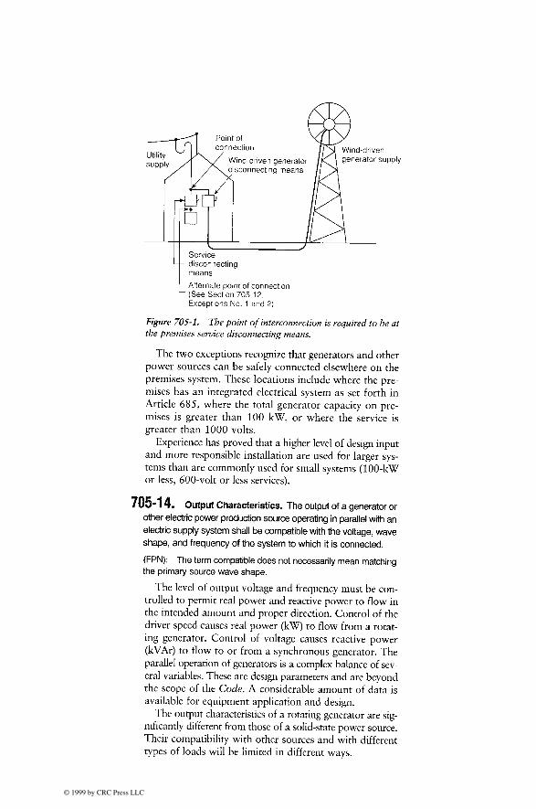
© 1999 by CRC Press LLC
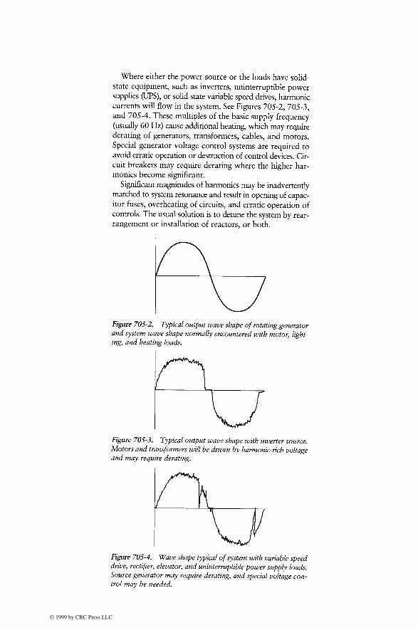
© 1999 by CRC Press LLC

© 1999 by CRC Press LLC

© 1999 by CRC Press LLC

© 1999 by CRC Press LLC

© 1999 by CRC Press LLC
A
PPENDIX
2
Sources of Further Information
on Renewable Energy
U.S. National Renewable Energy Laboratory (NREL)
Technical Inquiry Service1617 Cole BoulevardGolden, CO 80401Phone: (303) 275-4099Fax: (303) 275-4091
NREL offers a number of outreachservices, ranging from consumerinformation clearinghouses to elec-tronic bulletin boards, to its variousaudiences. The following is a list ofthese informative resources forwind, solar, and all other renewableenergy.
Electronic Information Server
This service provides general andtechnical information about NRELand may be accessed through Gopherat gopher.nrel.gov or through theWeb at htltp:
//
www.nrel.gov or viamodem at (303) 275-INFO.
Document Distribution Service
The DDS is the central repository fortechnical documents published byNREL.
Phone: (303) 275-4363Fax: (303) 275-4053E-mail: [email protected]
Energy Efficiency and Renewable Energy Clearinghouse
EREC provides information andtechnical assistance on subjectsrelated to energy efficiency andrenewable energy technologies.
P.O. Box 3048Merrifield, VA 22116Phone: (800) 363-3732TDD: (900) 273-2957BBS: (800) 273-2955E-mail: [email protected]
Energy Efficiency and Renewable Energy Network
This electronic service on the Inter-net serves as a gateway and reposi-tory of multimedia information onenergy efficiency and renewableenergy technologies.
Phone: (900) 363-3732Web: http:
//
www.eren.doe.gov

© 1999 by CRC Press LLC
Renewable Electric Plant Information System
REPIS, which is supported by DOE’sOffice of Utility Technologies, is anelectronic database of core informa-tion on grid-connected renewableelectric plants in the United States.RFPIS contains information on morethan 103,000 megawatts of installedrenewable capacity; approximately89 percent of which is hydroelectric.
Phone: (303) 275-4643Fax: (303) 275-4611E-mail: [email protected]
Renewable Resource Data Center
RREDC is the on-line informationdistribution service for the ResourceAssessment Program at NREL. Spon-sored by DOE, RREDC providesinformation about a variety of renew-able resources in the United States.The information includes publica-tions, data, maps, algorithms, andlinks to other sources of renewableenergy data.
Phone: (303) 275-4638Web: http:
// rredc.nrel.gov
Technical Inquiry Service
The TIS informs the scientific, indus-trial, and business communitiesabout NREL’s R&D activities andthose of NREL subcontractors.
Phone: (303) 275-4065Fax: (303) 275-4091E-mail: [email protected]
Technology and Business Ventures Office
Access to collaborative and spon-sored research, cost-shared subcon-tracts, NREL facilities, visiting re-searcher program, and cooperativeresearch and development agree-ments is available to individuals andbusinesses through this office.
Phone: (303) 275-3008Fax: (303) 275-3040E-mail: [email protected]: http:
//
www.nrel.gov
Visitors Center
The NREL visitor center provides aninteractive environment in whichyou can explore how solar, wind, andother types of renewable resourcescan provide energy to your industry,farm, community, and home.
Phone: (303) 384-6566E-mail: [email protected]

© 1999 by CRC Press LLC
Solar Energy Information Sources
American Solar Energy Society2400 Central AvenueBoulder, CO 80301, USAPhone: (303) 443-3130Fax: (303) 443-3212
British Photovoltaic AssociationThe Warren, Bramshill RoadEversley, Hamshire RG27 OPRUnited KingdomPhone: +44 (0) 118 932 4418Fax: +44 (0) 118 973 0820
Solar Trade Association LtdPengillan, Lerryn, LostwithielCornwall, United Kingdom
Manufacturers of Solar Cells and Modules in the U.S.A.
Advanced Photovoltaic Systems Inc.PO Box 7093Princeton, NJ 08543
Applied Solar Energy Corporation15751 East Don Julian RoadCity of Industry, CA 91746
ASE Americas, Inc.4 Suburban Park DriveBillerica, MA 01821
AstroPower, Inc.Solar ParkNewark, DE 19716-2000
ENTECHPO Box 612DFW Airport, TX 75261
EPV Energy PhotovoltaicsPO Box 7456Princeton, NJ 08543
Evergreen Solar49 Jones RoadWaltham, MA 02154
Iowa Thin Film TechnologiesISU Research Park #607Ames, IA 50010
SunPower Corporation430 India WaySunnyvale, CA 94086
SunWatt CorporationRFD Box 751Addison, ME 04606
Kyocera America, Inc.8611 Balboa AvenueSan Diego, CA 92123
A.Y. McDonald Mfg. Co.4800 Chavenelle Road-Box 508Dubuque, IA 52004-0508
Midway Labs, Inc.2255 East 75th StreetChicago, IL 60649
Sanyo Energy Corporation2001 Sanyo AvenueSan Diego, CA 92073
Siemens Solar Industries4650 Adohr LaneCamarillo, CA 93011
Solarex Corporation630 Solarex CourtFrederick, MD 21701
Solec International, Inc.12533 Chadron AvenueHawthorne, CA 90250

© 1999 by CRC Press LLC
Spire CorporationOne Patriots ParkBedford, MA 01730
Tideland Signal Co.PO Box 52430Houston, TX 77052
United Solar Systems Corporation9235 Brown Deer RoadSan Diego, CA 92121-2268
Utility Power Group9410 DeSoto Avenue, Unit GChatsworth, CA 91311

© 1999 by CRC Press LLC
Wind Energy Information Sources
As wind energy technology gains more widespread acceptance as an eco-nomically and technically viable resource, an increasing number of peoplerepresenting electric utilities, the news media, the research community, polit-ical and regulatory leaders, and local communities are searching for up-to-date, accurate information on this clean, renewable energy resource. The fol-lowing sources can provide a range of general and technical informationabout wind.
American Wind Energy Association(AWEA)122 C Street, NW, Fourth FloorWashington, D.C. 20001Phone: (202) 383-2500Publications: (202) 383-2520Fax: (202) 383-2505
Energy Efficiency & Renewable Energy NetworkPhone: (800) 363-3732
This electronic service on the internetserves as a gateway and repository ofmultimedia information on energyefficiency and renewable energytechnologies.
National Climatic Data Center151 Patton Avenue, Room 120Asheville, NC 28801-2733Phone: (704) 271-4800Fax: (704) 271-4876
National Wind Technology Center1617 Cole BoulevardGolden, CO 80401Phone: (303) 384-6900Fax: (303) 384-6901
National Technical Information ServiceU.S. Department of Commerce5285 Port Royal RoadSpringfield, VA 22161Phone: (703) 487-4650
Sandia National LaboratoriesP.O. Box 5800-MS 0899Albuquerque, NM 87185General Phone: (505) 845-0111Technical Info.: (505) 845-8287
National Institute of Science & TechnologyEnergy Inventions & InnovationsU.S. Department of CommerceRoom Al15, Building 411Gaithersburg, MD 20899-0001Phone: (301) 975-5500

© 1999 by CRC Press LLC
University Wind Energy Programs in the U.S.A.
A number of universities offer courses in renewable energy technologythrough environmental science or engineering departments. In addition toclasses, they work with industry partners to conduct valuable research. Insti-tutions offering specific wind energy curriculum and research programsinclude the following:
Alternative Energy InstituteWest Texas A&M UniversityP.O. Box 248Canyon, TX 79016Phone: (806) 656-2295
University of ColoradoElectrical & Computer EngineeringDepartmentCampus Box 425Boulder, CO 80309Phone: (303) 492-7010
Montana State UniversityChemical Engineering Department302 Cableigh HallBozeman, MT 59717Phone: (406) 994-4543
New Mexico State UniversitySouthwest Technology DevelopmentInstituteDept. 3 SOLARP.O. Box 30001Las Cruces, New Mexico 88003-9001Phone: (505) 646-1846
Ohio State UniversityAero and Astronautical Research2300 West Case RoadColumbus, OH 43220Phone: (614) 292-5491
Oregon State UniversityMechanical Engineering DepartmentCorvallis, OR 97331Phone: (503) 737-2218
Southwestern Technical College401 West StreetJackson, MN 56143Phone: (507) 847-3320 xi7i
Tennessee State University3500 John A. Merritt BoulevardNashville, TN 37209-1561Phone: (615) 320-3268
Tennessee Technological UniversityDepartment of Mechanical EngineeringCookeville, TN 38505-5014Phone: (615) 372-3273
University of ArizonaAME DepartmentTucson, AZ 85721Phone: (602) 621-2235
University of MassachusettsRenewable Energy Research LaboratoryCollege of EngineeringE Lab BuildingAmherst, MA 01003Phone: (413) 545-4359
University of Northern IowaIndustrial Technology CenterCedar Falls, IA 50614-0178Phone: (319) 273-2756

© 1999 by CRC Press LLC
University of Texas, El PasoMechanical Engineering Department500 W. University AvenueEl Paso, TX 79968-0521Phone: (915) 747-5450
University of UtahMechanical Engineering DepartmentSalt Lake City, UT 84112Phone: (801) 581-4145

© 1999 by CRC Press LLC
Periodicals on Wind Energy
Wind Energy WeeklyAmerican Wind Energy Association122 C Street. NW, Fourth FloorWashington, D.C. 20001Phone: (202) 383-2500
Published 50 times a year, WindEnergy Weekly provides up-to-dateinformation on utility requests forproposals, federal & state regulatoryactivity, project development, inter-national business opportunities, andenergy and environmental policy.
Home Power MagazineP.O. Box 520Ashland, OR 97520Phone: (916) 475-3179
This bimonthly magazine providesinformation about residential windsystems as well as information onother renewable technologies andproducts for residential use.
Independent Energy620 Central Avenue, NorthMilaca, MN 56353Phone: (612) 983-6892
Published 10 times a year, this mag-azine provides information for theindependent power industry andincludes periodic updates on thewind industry.
Wind Energy Technology: Generat-ing Power From the WindNational Technical Information ServiceU.S. Department of Commerce5285 Port Royal RoadSpringfield, VA 22161
This bimonthly publication providescurrent worldwide information onwind turbine design, performance,wind resource ident ificat ion ,legal/institutional implications, andenvironmental aspects of windpower.
Windpower MonthlyP.O. Box 496007, Suite 217Redding, CA 96099Phone: (415) 775-1985
This Danish magazine provides up-to-date information on all aspects ofthe international wind industry.
WindDirectionsEuropean Wind Energy Association26 Spring StreetLondon W2 1JAUnited KingdomPhone: +44 (0) 171 402 7122Fax: +44 (0) 171 402 7125E-mail: [email protected]: http:
//
www.ewea.org
WindDirections contains currenttechnical and commercial informa-tion on wind power plants and tech-nologies throughout the world.

© 1999 by CRC Press LLC
International Wind Energy Associations
British Wind Energy AssociationLincoln’s Inn House42 KingswayLondon WC2B 6EXUNITED KINGDOMPhone: +44 171 404 3433Fax: +44 171 404 3432
Canadian Wind Energy Association2415 Holly Lane, Suite 250Ottawa, Ontario KIV 7P2CANADAPhone: (613) 736-9077
Danish Wind Power Association(Wind Turbine Owners’ Organization)Phone: +45 53 83 13 22Fax: +45 53 83 12 02
European Wind Energy Association26 Spring streetLondon W2 1JAUNITED KINGDOMPhone: +44 (0) 171 402 7122Fax: +44 (0) 171 402 7125E-mail: [email protected]: http:
//
www.ewea.org
Finnish Wind Power AssociationPhone: +358 0 456 6560Fax: +358 0 456 6538
FME Groep Windenergic(Dutch wind energy trade association)Phone: +31 79 353 1100Fax: +31 79 353 1365
French Wind Energy Association63 Collet de DarboussonValbonne 06560FRANCEPhone: +33 93 65 0970
German Wind Energy AssociationDorfangerweg 15Unterfoehring 85774GERMANYPhone: +49 899506411
Gujarat Energy Development AgencySuraj Plaza II, 2
nd
Floor, Sayaji GunjVadodara – 390 005, INDIAFax: +91-265-363120
Hellenic Wind Energy Association(Greece)Phone: +30 1 603 9900Fax: +30 1 603 9905
Indian Renewable Energy Develop-ment AgencyCore-4 A, East Court, 1st FloorHabitat Center Complex, Lodi RoadNew Delhi-110 003, INDIAFax: +91-11-460-2855
Indian Ministry of Non-Conven-tional Energy SourcesBlock 14, CGO ComplexLodi RoadNew Delhi – 110 003, INDIAFax: +91-11-436-1298
Institute Catalia d’EnergiaAvenue Diagonal, 453 Bis. Atic08036 Barcelona, SPAINFax: +343-439-2800
Norwegian WindEnergy AssociationPhone:+47 66 84 63 69Fax: +47 66 98 11 80
Romanian Wind Energy AssociationPhone: +40 1 620 67 30/260Fax: +40 1 312 93 15

© 1999 by CRC Press LLC
Risø National LaboratoryPO Box 494000 Roskilde, DENMARKTel: + 45 46 77 50 35Fax: + 45 46 77 50 83Web: www.risoe.dk/amv/index.html
Tata Energy Research InstituteDarbari Seth Block, Habitat PlaceNew Delhi – 110 003, INDIAPhone: +91-11-460-1550
Fax: +91-11-462-1770E-mail: [email protected]: http:
//
www.teriin.org
Vindmolleindustrien(Association of Danish wind turbines Manufacturers)Norre Voldegadc 48, OPGB.Kobenhaven K DK-1358DENMARKPhone: +45 33 –779988

© 1999 by CRC Press LLC
Wind Power System Suppliers in the U.S.A.
The following is a partial list of wind turbine manufacturers and developersin the U.S.A. A complete list and company profile can be obtained from:
American Wind Energy Association
122 C St., NW, Fourth FloorWashington, D.C. 20001Phone: (202) 383-2520Fax: (202) 383-2505 fax
E-mail: [email protected]__________________________________________________________________
Atlantic Orient Corp.P.O. Box 1097Norwich, VT 05055Phone: (802) 649-5446Fax (801) 649-5404
Bay Winds1533 Kimball StreetGreen Bay, WI 54302Phone: (920) 468-5500
Bergey Windpower Company2001 Priestley AvenueNorman, OK 73069Phone: (405) 364-4212Fax: (405) 364-2078E-mail: [email protected]
Lake Michigan Wind & Sun Ltd.East 3971 Bluebird RoadForestville, WI 54213-9505Phone: (414) 837-2267Fax: (414) 837-7523E-mail: [email protected]
Southwest Windpower2131 North First StreetFlagstaff, AZ 86001Phone: (520) 779-WINDFax: (520) 779-1485Web: http:
//
www.windenergy.com
Wind Turbine Industries Corp.16801 Industrial Circle, SEPrior Lake, MN 55372Phone: (612) 447-6064Fax: (612) 447-6050
WindTech International, L.L.C.P.O. Box 27Bedford, NY 10506Phone: (914) 232-2354Fax: (914) 232-2356E-mail: [email protected]: http:
//
www.windmillpower.com
World Power Technologies, Inc.19 N. Lake AvenueDuluth, MN 55802Phone: (218) 722-1492Fax: (218) 722-0791E-mail: [email protected]: http:
//
www.webpage.com/wpt/

© 1999 by CRC Press LLC
Utility-scale wind turbines manufacturers and developers
Advanced Wind TurbinesNEG Micon U.S.A., Inc.Mitsubishi Heavy IndustriesNedWind (Netherlands)Vestas American WindWind Turbine CompanyEnron Wind Corporation
Cannon Energy CorporationEnergy Unlimited, Inc.FORAS Service CompanySeaWest Energy CorporationTomen Power CorporationYork Research Corporation

© 1999 by CRC Press LLC
European Wind Energy Association
List of the EWEA Members as of September 1998. Reproduced with permis-sion from EWEA Head Office
European Wind Energy Association
26 Spring StreetLondon, W2 1JA, UKTel: +44 171 402 7122Fax: +44 171 402 7125
E-mail: [email protected]: www.ewea.org
Manufacturers and Developers
ABB Motors OYPL 63365101 VaasaFinlandTel: + 358 10 22 4000Fax: + 358 10 22 47372
Aerpac b.v.PO Box 167Bedrijvenpark Twente 96Almelo 7600 AThe NetherlandsTel: + 31 546 549 549Fax: + 31 546 549 599E-mail: [email protected]
ATV EntrepriseActipole St Charles13710 FuveauFranceTel: + 33 4 42 29 14 62Fax: + 33 4 42 29 14 61
A/S Wincon West WindHedemoelle Erhvervsvej 4DK-8850 BjerringbroDenmarkTel: + 45 86 68 1700Fax: +45 86 68 1734
Bonus Energy A/SFabriksvej 47330 BrandeDenmarkTel: + 45 97 18 11 22Fax: + 45 97 18 30 86E-mail: [email protected]
Desarrollos Eolicos SAAvenida de la Buhaira, 241018 SevillaSpainTel: + 34 95 493 7000Fax: + 34 95 493 7017
Ecotecnia SCCLAmistat 23 1st08005 BarcelonaSpainTel: +34 93 225 7600Fax: +34 93 221 0939E-mail: [email protected]: www.ecotecnia.com
Enercon GmbHDreekamp 5D-26605 AurichGermanyTel: +49 421 24 9920Fax: +49 421 24 9960E-mail: [email protected]: www.enercon.de

© 1999 by CRC Press LLC
KK Electronic A/SCypresvej 67400 HerningDenmarkTel: + 45 97 22 1033Fax: + 45 97 21 1431E-mail: [email protected]: www.kk-electronic.dk
Italian Vento Power Corp. (IVPC)Via Circumvallazione 54/H83100 AvellinoItalyTel: + 39 825 781 473Fax: + 39 825 781 472E-mail: [email protected]
L M Glasfiber A/SRolles Mollevej 16640 LunderskovDenmarkTel: + 45 75 58 51 22Fax: + 45 75 58 62 02E-mail: [email protected]: www.lm.dk
National Windpower LtdRiverside House, MeadowbankFurlong RoadBourne End, SL8 5AJ, UKTel: + 44 1628 532300Fax: + 44 1628 531993Web: www.enterprise.net
/
manxwind.nwp.htm
NedWind bvPostbus 1183910 AC RhenenThe NetherlandsTel: 31 317 619 004Fax: 31 317 612 129E-mail: [email protected]: www.nedwind.nl
NEG Micon A/SAlsvej 21DK-8900 RandersDenmarkTel: + 45 87 10 5000Fax: + 45 87 10 5001E-mail: [email protected]
NEG Micon (UK) LtdTaywood House, 345 Ruislip RoadSouthall, Middlesex, UB1 2QXUKTel: + 44 181 575 9428Fax: + 44 181 575 8318
Nordex Balke-Durr GmbHSvindbaek7323 GiveDenmarkTel: + 45 75 73 44 00Fax: + 45 75 73 41 47E-mail: [email protected]: www.nordex.dk
Renewable Energy Systems LtdPilgrims Lodge, Holywell HillSt Albans, Herts, AL1 1ER, UKTel: + 44 1727 797900Fax: + 44 1727 797929Web: www.res-ltd.com
Risø National LaboratoryPO Box 494000 RoskildeDenmarkTel: + 45 46 77 50 35Fax: + 45 46 77 50 83Web: www.risoe.dk
/
amv
/
index.html
Riva Wind TurbinesVia Emilia Ponente 7240133 BolognaItalyTel: + 39 51 413 0511Fax: + 39 51 413 0650

© 1999 by CRC Press LLC
SeaWest Energy Corporation1455 Frazee Road, Suite 900CA 9210, San DiegoUSATel: +1 619 293 3340Fax: +1 619 293 3347E-mail: [email protected]
Stork Product EngineeringPO Box 3791000 AJ AmsterdamThe NetherlandsTel: + 31 205 563 444Fax: + 31 205 563 556
Valmet Power Transmission IncPO Box 15840101 JyvaskylaFinlandTel: + 358 14 296 611Fax: + 358 14 296 868
Vergnet SA6 Rue Henri Dunant45410 IngreFranceTel: + 33 2 38 227 500Fax: + 33 2 38 227 522E-mail: [email protected]
Vestas Wind Systems A/SSmed Hanseen Vej 276940 LemDenmarkTel: + 45 97 34 11 88Fax: + 45 97 34 14 84E-mail: [email protected]: www.vestas.dk
West S.P.A.Alenia/WESTViele Maresciallo Pilsudsky 92I-00131 RomaItalyTel: + 39 6 80 77 88 33Fax: + 39 6 80 77 88 48
Western Windpower LtdStroud House, Russell StreetStroud, GloucestershireGL5 3AN, UKTel: + 44 1453 579408Fax: + 44 1453 766770
Zond International LtdPrince Consort House27-29 Albert EmbankmentLondonSE1 7TJ, UKTel: + 44 171 793 2800Fax: + 44 171 820 3401E-mail: [email protected]: www.zond.com
Research & Consultancy
Bond PearceBallard HouseWest Hoe RoadPlymouth, PL1 3AE, UKTel: + 44 1752 266633Fax: + 44 1752 225350
ECN Renewable EnergyPostbus 11755 ZG PettenThe NetherlandsTel: + 31 224 56 41 84Fax: + 31 224 56 32 14Web: www.ecn.nl
Elsamprojekt A/SKraftvaerksvej 537000 FredericiaDenmarkTel: + 45 79 23 3333Fax: + 45 75 56 4477Web: www.elsamprojekt.dk
Garrad Hassan & Partners LtdThe Coach HouseFolleigh Lane, Long AshtonBristol, BS18 9JB, UKTel: +44 1275 394360Fax: + 44 1275 394361

© 1999 by CRC Press LLC
Banque Paribas37 Place du Marche, St Honore75001 ParisFranceTel: + 33 1 42 98 77 38Fax: + 33 1 42 98 19 89
BTM Consult A/SI C Christensens Alle 16950 RingkobingDenmarkTel: + 45 97 32 5299Fax: + 45 97 32 5593E-mail: [email protected]: www.home4.inet.tele.dk
/
btmc-wind
China Fulin Windpower Develop-ment Corp.No 1, Dongbinhe RoadYouanmenwai, Fengtai District100054 BeijingP.R. ChinaTel: + 86 10 635 304 17Fax: + 86 10 635 304 15
EoleBP 7213702 La Ciotat CedexFranceTel: + 33 4 42 08 14 66Fax: + 33 4 42 08 16 56E-mail: [email protected]
ESD LtdOvermoor FarmNestonWiltshire, SN13 9TZ, UKTel: + 44 1225 816804Fax: + 44 1225 812103Web: www.esd.co.uk
Espace Eolien Developpement16 Rue Faidherbe59000 LilleFrance
Tel: + 33 3 20 74 04 00Fax: + 33 3 20 74 04 07Web: www.espace-eolien.fr
Grant Rush & Co LtdPreston Park StationClermont RoadBrighton, BN1 6SG, UKTel: + 44 1273 540410Fax: + 44 1273 504028E-mail: [email protected]
Institutt for EnergiteknikkPO Box 402007 KjellerNorwayTel: + 47 63 80 6180Fax: + 47 63 81 2905Web: www.ife.no
La Compagnie du VentHorizon 21, 650 rue Louis LepineLe Millenaire, 34000 MontpellierFranceTel: + 33 4 99 52 64 70Fax: + 33 4 99 52 64 71E-mail: [email protected]: perso.wanadoo.fr
/
cabinet.ger-ma
LMW Renewables BVPO Box 2793770 AG BarneveldThe NetherlandsTel: + 31 342 421 986Fax: + 31 342 421 759
Mees Pierson N.V.Camomile Court23 Camomile StreetLondon, EC3A 7PPUKTel: + 44 171 444 8712Fax: + 44 171 444 8810

© 1999 by CRC Press LLC
NRG Systems Inc.110 Commerce Street05461 Hinesburg, VTUSATel: +1 802 482 2255Fax: +1 802 482 2272
Shell International RenewablesHead Biomass & WindShell CentreLondon, SE1 7NA, UKTel: + 44 171 934 3386Fax: + 44 171 934 7470
Synergy Power Corporation20/F Wilson House19-27 Wyndham Street, CentralHong KongTel: +852 2846 3168Fax: +852 2810 0478E-mail: [email protected]
Teknikgruppen ABPO Box 2119121 SollentunaSwedenTel: + 46 8 444 5121Fax: + 46 8 444 5129
Tractebel Energy EngineeringAvenue Ariane 7B-1200 BrusselsBelgiumTel: +32 2 773 8345Fax: +32 2 773 9700
Trillium Pakistan (PVT) Ltd10th Floor, AWT Plaza5 The MallRawapindi-Cantt.PakistanTel: + 92 51 56 21 07Fax: + 92 51 56 80 44E-mail: [email protected]
Tripod Consult APSGladsaxe Mollevej 212860 SoborgDenmarkTel: + 45 39 66 66 22Fax: + 45 39 66 66 99E-mail: [email protected]
National Associations
APPAParis 20508008 BarcelonaSpainTel: + 34 3 414 22 77Fax: + 34 3 209 53 07E-mail: [email protected]
Austrian Wind Energy AssociationIG Windkraft -OsterreichMariahilferstrasse 89/221060 ViennaAustriaTel: + 43 1 581 70 60Fax: + 43 1 581 70 61E-mail: [email protected]
British Wind Energy Association26 Spring StreetLondonW2 1JA, UKTel: + 44 171 402 7102Fax: + 44 171 402 7107E-mail: [email protected]: www.bwea.com
Bundesverband WindenergieAm Michelshof 8-1053177 BonnGermanyTel: + 49 228 35 22 76Fax: + 49 228 35 23 60E-mail: [email protected]: www.wind-energie.de

© 1999 by CRC Press LLC
Danish Wind Turbine Manufactur-ers Assoc.Vester Voldgade 106DK-1552 CopenhagenDenmarkTel: + 45 33 73 0330Fax: + 45 33 73 0333E-mail: [email protected]: www.windpower.dk
Danmarks VindmolleforeningEgensevej 24Postboks 454840 Nr AlstevDenmarkTel: + 45 54 43 13 22Fax: + 45 54 43 12 02E-mail: [email protected]: www.danmarks-vindmoelle-forening.dk
Dutch Wind Energy BureauPostbus 106800AA ArnhemThe NetherlandsTel: + 31 26 355 7400Fax: + 31 26 355 7404
Finnish Wind Power AssociationPO Box 846FIN-00101 HelsinkiFinlandTel: + 358 9 1929 4160Fax: + 358 9 1929 4129Web: www.fmi.fi
Fordergesellschaft Windenergie E.V.Elbehafen25541 BrunsbuttelGermanyTel: + 49 48 52 83 84 16Fax: + 49 48 52 83 84 30E-mail: [email protected]
France Energie EolienneInstitut Aerotechnique15 rue Marat78210 Saint-Cyr-l’EcoleFranceTel: + 33 1 30 45 86 01Fax: + 33 1 30 58 02 77
Hellenic Wind Energy Associationc/o PPC, DEME10 Navarinou Str10680 AthensGreeceTel: + 30 1 36 21 465Fax: + 30 1 36 14 709
Irish Wind Energy AssociationKellystownSlane, County MeathIrelandTel/fax: + 353 41 267 87
ISES – Francec/o ADEME500 Route des Lucioles05560 ValbonneFranceTel: + 33 4 93 95 79 18Fax: + 33 4 93 95 79 87
ISES – ItaliaP.zza Bologna, 22 A/900162 RomaItalyTel: + 39 6 44 24 9241Fax: + 39 6 44 24 9243E-mail: [email protected]: www.isesitalia.it
Japanese Wind Energy Associationc/o Mechanical Engineering Lab.1-2 Namiki, Tsukuba305 Ibaraki-KenJapanTel: + 81 298 58 7014Fax: + 81 298 58 7275

© 1999 by CRC Press LLC
Netherlands Wind Energy AssociationTU Delft, Institute for WindStevinweg 12628 CN, DelftThe NetherlandsTel: + 31 15 27 85 178Fax: + 31 15 27 85 347
Romanian Wind Energy AssociationPower Research Institute BdEnergeticienilor 876619 BucharestRomaniaTel/fax: + 40 1 32 14 465or + 40 1 32 22 790
Turkish Wind Energy AssociationEiE Idaresi Genel MudurluguEskisehir Yolu 7km No. 16606520 AnkaraTurkeyTel: + 90 312 287 8440Fax: + 90 312 287 8431

© 1999 by CRC Press LLC
Acronyms
ASES American Solar Energy SocietyAWEA American Wind Energy AssociationAh Ampere·hour of the battery capacityBIPV Building Integrated PhotovoltaicsC/d Charge/discharge of the batteryDOD Depth of Discharge of the battery from its rated capacityDOE Department of EnergyECU European Currency UnitEDF Energy Delivery FactorEPRI Electric Power Research InstituteEWEA European Wind Energy AssociationGW Gigawatt (10
9
watts)IEA International Energy AgencykW KilowattkWh Kilowatt·hourMW MegawattMWh Megawatt·hourNEC National Electric CodeNREL National Renewable Energy LaboratoryPV PhotovoltaicQF Qualifying FacilitySOC State of Charge of the batteryTHD Total Harmonic Distortion in measuring the quality of powerUCE Unit Cost of Energy

© 1999 by CRC Press LLC
Conversion of Units
The information contained in the book came from many sources and manycountries using different units in their reports. The data are kept in the formthey were received by the author rather than converting to a common systemof units. The following is the conversion table for the most commonly usedunits in the book.
To change from Into Multiply by
mile per hour meter/second 0.447knot meter/second 0.514mile kilometer 1.609foot meter 0.3048inch centimeter 2.540pound kilogram 0.4535Btu watt·second 1054.4Btu kilowatt·hour 2.93 ·10
–4
Btu/ft
2
watt·second/m
2
11357Btu/hr watts 0.293Btu/ft
2
/hr kW/meter
2
3.15 ·
10
–7
Btu/h·ft
2
·°F watt/m
2
°C 5.678horsepower watts 746gallon of oil (U.S.) kWh 42gallon (U.S.) liters 3.785barrel of oil Btu 6 · 10
6
barrel gallons (U.S.) 42