Abstract—The objective of this paper was to provide

directions on the design phase and construction of a multistage

bipolar junction transistor amplifier circuit, that holds certain

specifications for the product to function. The multistage

amplifier consisted of three stages, hand calculations, P-Spice

simulator and the building of the circuit/lab measurements.

Overall the amplifier was design to have a numerical gain of 1100

with an output swing of 12 volts peak to peak.

Index Terms— Bipolar Junction Transistor (BJT), Multistage,

Emitter, Base, and Collector

I. INTRODUCTION

HIS experiment was used to design a BJT (Bipolar

Junction Transistor) amplifier using Q2N3904. The

following are the specifications for the design:

Power Consumption

The process for this BJT design was to create a gain of 1100

V/V, which has three different stages. The first stage was to

design a circuit from the specification values called hand

calculations. The second stage was to design the amplifier on

P-Spice simulator. P-Spice demonstrated results for the

amplifier circuit and confirmed the solutions from the hand

calculations. The last stage was to duplicate the design from P-

Spice to the breadboard in the lab. The following will be

explained in the report hand calculations, P-Spice Simulation,

Ethan Miller Author, is with the Electrical Engineering Department, University of North Carolina at Charlotte, Charlotte, NC 7 28262 USA

(E-mail: emille76@uncc.edu).

Charles Truong Author, is with the Electrical Engineering Department,

University of North Carolina at Charlotte, Charlotte, NC 7 28262 USA

(E-mail: crtruong2@uncc.edu).

and laboratory measurements/actual circuit built.

II. AMPLIFIER

Amplifiers are used to amplify the signal input, an

electronic device that increases the power of a signal. The BJT

transistor has three-terminals, and is often called a

semiconductor device. BJT basic principle involves the use of

controlling the current flowing in the third terminal, which can

be realized as a controlled source. There are to two types of

BJT’s, one type is called NPN and the other type is called

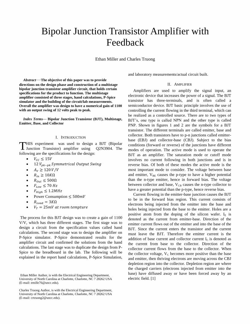
PNP. Shown in figures 1 and 2 are the symbols for a BJT

transistor. The different terminals are called emitter, base and

collector. Both transistors have to p-n junctions called emitter-

base (EBJ) and collector-base (CBJ). Subject to the bias

conditions (forward or reverse) of the junctions have different

modes of operation. The active mode is used to operate the

BJT as an amplifier. The saturation mode or cutoff mode

involves no current following in both junctions and is in

reverse bias. Of both of these modes the active mode is the

most important mode to consider. The voltage between base

and emitter, VBE causes the p-type to have a higher potential

than the n-type emitter, hence in forward bias. The voltage

between collector and base, VCB causes the n-type collector to

have a greater potential than the p-type, hence reverse bias.

Current flowing in the emitter-base junction causes the BJT

to be in the forward bias region. This current consists of

electrons being injected from the emitter into the base and

holes being injected from the base to the emitter. Holes are a

positive atom from the doping of the silicon wafer. IE is

denoted as the current from emitter-base. Direction of the

emitter current flows out of the emitter and into the base of the

BJT. Since the current enters the transistor and the current

must leave the BJT. Therefore the emitter current is the

addition of base current and collector current IC is denoted as

the current from base to the collector. Direction of the

collector current flows from the base to the collector. When

the collector voltage, VC becomes more positive than the base

and emitter, then thriving electrons are moving across the CBJ

depletion region into the collector. Depletion region are where

the charged carriers (electrons injected from emitter into the

base) have diffused away or have been forced away by an

electric field. [1]

Bipolar Junction Transistor Amplifier with

Feedback

Ethan Miller and Charles Truong

T

Figure 1: NPN BJT Transistor

Figure 2: PNP BJT Transistor

Current in the base denoted as IB is due to the holes injected

from the base into the emitter region and due to the holes

provided by the exterior circuit to replace the holes lost from

the base. The base current total is the addition of the holes

injected from the base to collector and emitter to base. As a

result the base current is in terms of beta denoted as . Beta or

common-emitter current gain is the transistor parameter,

usually in the range of 50 to 200. This beta is influence by the

width of base region and the doping’s of the base region. [2]

III. LOAD LINE ANALYSIS

AC (alternating current) and DC (direct coupled) load lines

were part of the hand calculations stage of the design. Here the

y-axis of the graph represents the collector current and the x-

axis represents voltage from the collector to the emitter. The

purpose of the load line was to define the q-point (quiescent

point). The place of the q-point was determined to by the

swing specification of 12V peak to peak, or where the two

load lines intersect on the graph. Also taken into consideration

was to make sure the amplifier circuit was not in saturation

mode, as the signal departs through the amplifier.

IV. HAND ANALYSIS

The deciding values that were used for the amplifier circuit

was first to be chosen from the q-point. The q-point was

determined by the AC and DC load lines. Other calculations

that were solved are the following DC biasing, AC vs. DC

load line, Voltage gain, R-input, R-output, power

consumption, swing for the circuit and the frequency at low

and high end of the voltage gain. Current and Voltages

through the collector, base and emitter were solved by

determining the bias conditions for BJT transistor. Hand

calculations are found in appendix A. [3]

V. P-SPICE ANALYSIS

Components values were selected from the hand

calculations to ensure the amplifier circuit had the correct

specifications and the amplifier was in the forward bias

region. Graphs were then taken to show the accuracy of

specifications calculated from the hand analysis were correct.

The following graphs were taken are voltage gain, input and

output resistance as a function of frequency, transient response

of the output voltage and current at an input frequency of 10

kHz (Hertz), frequency response of the low and high cutoff

values, frequency response as a function of temperature,

midband voltage gain, frequency response as a function of the

load resister. P-Spice analyses are found in appendix C.

VI. ACTUAL CIRCUIT

The last stage of the design was to build the amplifier on a

breadboard from the values that were hand calculated and

compared the hand calculations to P-Spice analysis with a

minimum of 5% error. Certain Equipment was used for this

lab. The following was the equipment used: function

generator, oscilloscope, power supply, and multimeter.

Oscilloscope displayed the input and output signal for the

amplifier circuit. Function generator purpose was to design an

input signal for the circuit. The multimeter was design to

measure the diverse voltages and current throughout the

circuit. The power supply was used to supply a voltage of 15

volts to the collector and base terminals for the BJT transistor.

The function generator provided did not go below 50mV

amplitude, so a voltage divider was built in order to fix the

problem. The voltage divider was built to have 5mV

amplitude input voltage, so the gain would have 1100 v/v. P-

Spice circuit diagrams are shown in appendix B, lab

measurements are shown in appendix E, and the lab graphs are

shown in appendix F. [4] A feedback was applied to the

circuit to ensure the stability of the circuit. The feedback was

found to be 800 ohms to reduce the overall gain by a factor of

10. A feedback of series-series was applied the circuit.

APPENDIX

Appendix A ……………………………Hand Analysis

Appendix B ……………………………Circuit Diagrams

Appendix C………………………………P-Spice Graphs

Appendix D...………………….……Small Signal Model

Appendix E …………………..…Measurements From Lab

Appendix F………………………………….Lab Graphs

VII. CONCLUSION

In conclusion, the experiment was found to have a gain of

2151 V/V, and a swing of 12.1 V/V. The following input and

output resisters were found to be 36.3 kΩ, 361 Ω. The power

consumption was set to 450 mW, to establish no current

forced back into the power supply. Rail voltage was to set 15

volts and the resister load was set to 3 kΩ. Other parameters

that were measured are the following 66 Hz low cutoff

frequency and 520 kHz high cutoff frequency.

VIII. REFERENCES

[1] E. Coates, "Learnabout-Electronics-Transistors,"

Learnabout-Electronics -Transistors, 12 June 2013.

[Online]. Available: http://www.learnabout-

electronics.org/bipolar_junction_transistors_05.php.

[Accessed 12 June 204].

[2] W. Foundation, "Biploar Junction Transister," Wikimedia

Foundation, 11 June 2014. [Online]. Available:

http://en.wikipedia.org/wiki/Bipolar_junction_transistor.

[Accessed 12 July 2014].

[3] A. S. Sedra and K. C. Smith, Microelectronic Ciruits, sixth

ed., New York: Oxford University, 2010.

[4] W. Storr, "Basic Electronic Tutorials," Electronics

Tutorials, 11 June 2014. [Online]. Available:

http://www.electronics-tutorials.ws/transistor/tran_1.html.

[Accessed 12 June 2014].

Appendix A

Av Calculations:

Rin Calculations:

Rout Calculations:

F Low Calculations:

F High Calculations:

Appendix B

Figure 3: BJT Amplifier Circuit with Feedback

Figure 4: DC Voltage

Appendix B

Figure 5: DC Current

Appendix C

Figure 6: Frequency Response Gain

Figure 7: Frequency Response Gain dB

Appendix C

Figure 8: Power at 10 kHz

Figure 9: Vout at 10 kHz

Appendix C

Figure 10: Iout at 10 kHz

Figure 11: Frequency Response Rin

Appendix C

Figure 12: Frequency Response Rout

Figure 3: Swing

Figure 13: Frequency Response as a Function of Rload

Appendix E

Figure 14: Frequency Response as a Function of Temperature

Figure 15: Frequency Response of Output Voltage Swing

Appendix D

Figure 16: AC Equivalent for Each Stage

Appendix E

Frequency (Hz) Rin (Ω) Rout (Ω) Vin ,pk-pk (mV)

Vout ,pk-pk (V)

Vout ,min (V)

Vout ,max (V)

Av (V/V)

10 51250 3613.636 111 4.6mv -2.3 2.3 .041441

70 51250 488.8889 111 8.6 -4.3 4.3 77.47748

100 51250 446.0432 109 9.8 -4.9 4.9 89.90826

1000 51250 386.2069 109 10.9 -5.3 5.5 101.862

10000 51250 372.4138 107 10.5 -5.1 5.3 101.9417

100000 19900 377.6224 103 10.5 -5.1 5.3 95.1453

1000000 1512.5 353.7415 103 9.8 -5.1 4.7 95.1456

1200000 1138.298 331.1258 103 9.4 -4.9 4.5 91.26214

2500000 467.1533 292.9936 101 5 -2.5 2.5 65.34653

F-Low 3db 68.3 HZ

F-High 3db 1.8 MHZ

Table 1: Frequency Sweep Lab Measurements

Hand Calculation Lab Measurements Percent Error

Rin (Ω) Rout (Ω) Rin (Ω) Rout (Ω) Rin (Ω) Rout (Ω)

39400 362.8 51250 372.4137931 30.07% 2.65%

Figure 17: Vout Swing Lab Measurements

Table 2: Percent Error Lab Measurements

Appendix F

0

10

20

30

40

50

60

70

80

90

100

110

5 50 500 5000 50000 500000 5000000

Vo

lta

ge

Ga

in

(V/V

)

Frequency (Hz)

Voltage Gain (Av)

Gain

Figure 18: Frequency Sweep Voltage Gain

Appendix F

400

5400

10400

15400

20400

25400

30400

35400

40400

45400

50400

10 100 1000 10000 100000 1000000

Inp

ut

Imp

eda

nce

(Ω

)

Frequenecy (Hz)

Input Impedance Input Impedance

Figure 19: Frequency Sweep Input Impedance

Appendix F

250 450 650 850

1050 1250 1450 1650 1850 2050 2250 2450 2650 2850 3050 3250 3450 3650

10 100 1000 10000 100000 1000000

Ou

tpu

t Im

ped

acn

e (Ω

)

Frequency (Hz)

Output Impedance Output …

Figure 20: Frequency Sweep Output Impedance