von Karman Institute for Fluid DynamicsLecture Series 1999-0330TH COMPUTATIONAL FLUID DYNAMICS

March 8 - 12, 1999LOW MACH NUMBER ASYMPTOTICS OF THE NAVIER-STOKESEQUATIONS AND NUMERICAL IMPLICATIONS

B. M�ullerUppsala University, Sweden

Low Mach Number Asymptotics of theNavier-Stokes Equations andNumerical ImplicationsB. M�ullerDepartment of Scienti�c Computing, Information Technology,Uppsala University, P.O. Box 120, S-751 04 Uppsala, SwedenAbstractLow Mach number asymptotics of the Navier-Stokes equations reveals the role of thelarge global thermodynamic pressure, the small acoustic pressure and the very small'incompressible' pressure. Solving for the changes of the conservative variables withrespect to stagnation conditions retains the conservative discretization and avoidsthe cancellation problem, when computing the small changes in low Mach number ow.Key words: Navier-Stokes equations, asymptotic analysis, low Mach number ow, aeroa-coustics, cancellation, perturbation formulation, �nite volume method, approximate Rie-mann solver.Notation: In this lecture, all physical quantities with superscript * are dimensional andall physical quantities without superscript * are nondimensional. Unless stated otherwise,the nondimensionalization (13) is used.IntroductionSpeaking, singing and playing a music instrument are pleasant examples of compressiblelow Mach number ow, unless they are considered as noise. Acoustics in gases and liquidsis not only a daily experience, but also has great scienti�c and technological signi�cance.Aerodynamic noise regulations have become more restrictive due to public demandscaused by increased transport of persons and goods and by increased environmental sen-sitivity. Thus, aeroacoustics has become a key issue in the design of airplanes, helicopters,trains, cars, engines, gas turbines, etc. The available computational power and emerg-ing numerical methods have recently led to computational aeroacoustics (CAA) as a newbranch of computational uid dynamics (CFD). Like CFD, CAA o�ers great potentialto complement theoretical and experimental aeroacoustic research. Therefore, Sir JamesLighthill foresees a \second golden age of aeroacoustics" [1].Since in many practical applications the sound generation is primarily determined bythe slow vorticity uctuations in a turbulent ow, there has been considerable interest inlow Mach number computational aeroacoustics. Crighton argues [2]:\First, why is there interest in low Mach number aeroacoustics at all, whether analytical,1

experimental or computational?...; unless the mean ow exceeds roughly twice the ambient speed of sound (...) theradiation is determined primarily by the slow temporal evolution of convected eddies; ...Second, why are we making a fuss about computational aeroacoustics?... The problem is that all numerical analysis procedures are inherently noisy (in theacoustic sense). ... the numerical procedure may actually be \noisier" than the ow! ...In aeroacoustics we are dealing with the minutest energy levels, compared with the whole ow - and moreover, with those energies on length scales O(M�1) larger than the scales ofthe \energy-containing eddies". Calculations of these lie, in energy and scale, far outsidethe range of conditions adequately resolved by standard CFD procedures. This is whatmakes computational aeroacoustics at low Mach number not merely a technologically, butalso a scienti�cally, important problem."However, it is not only aeroacoustics, which makes compressible low Mach number ow such an interesting problem. Even in hypersonic ow, there are low Mach numberregions in the vicinity of stagnation points and no-slip surfaces, at which the velocity iszero. Separated ow is often characterized by low Mach numbers. Whereas conventionalcompressible ow codes perform rather well for transonic ow, their accuracy and e�-ciency deteriorates considerably as the Mach number approaches zero [3]. Therefore, thecomputation of compressible low Mach number ow is an important issue in CFD bothfor steady and unsteady ow.In the �rst part of this lecture, low Mach number asymptotic analyses are performedto get better mathematical insight into the Navier-Stokes equations and better physicalunderstanding of the mechanisms they describe, as the Mach number M goes to zero.In the second part of this lecture, numerical implications are drawn from the asymp-totic analyses and from physical facts in low Mach number ow. The cancellation problemand its solution by the perturbation form of the Navier-Stokes equations are described indetail.The conclusions are stated in the third part.1 Low Mach Number Asymptotics of theNavier-Stokes Equations1.1 Review and OutlineLow Mach number asymptotics is used by Klainerman and Majda [4] for the Euler equa-tions and by Kreiss et al. [5] for the Navier-Stokes equations to prove the convergence ofthe compressible ow solutions to the incompressible ow solutions for M ! 0 under cer-tain conditions. Majda [6] employs low Mach number asymptotics to derive the equationsfor low Mach number combustion. The resonant interaction of small amplitude periodichigh frequency acoustic waves with entropy and vorticity waves is studied by Hunter etal. [7], Majda et al. [8], Almgren [9] and other authors using the method of multiplescales. Rehm and Baum [10] derive the low Mach number limit of the compressible Eulerequations for buoyant inviscid ow with heat release. For the low Mach number limit ofthe compressible Navier-Stokes equations, Fedorchenko [11] provides a number of exactsolutions. Employing multiple time and space scale expansions, Zank and Matthaeus [12]derive low Mach number equations from the compressible Navier-Stokes equations. Thesingle time scale, multiple space scale asymptotic analysis by Klein [13] yields insight intothe low Mach number limit behaviour of the compressible Euler equations and has been2

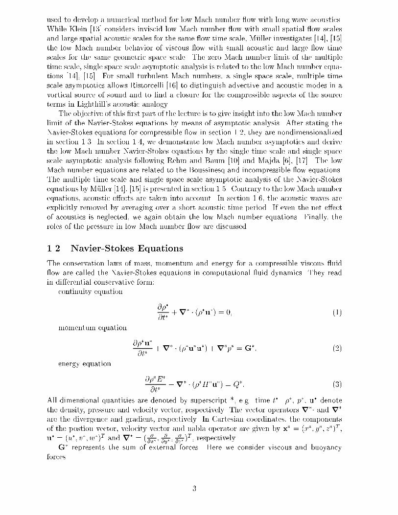
used to develop a numerical method for low Mach number ow with long wave acoustics.While Klein [13] considers inviscid low Mach number ow with small spatial ow scalesand large spatial acoustic scales for the same ow time scale, M�uller investigates [14], [15]the low Mach number behavior of viscous ow with small acoustic and large ow timescales for the same geometric space scale. The zero Mach number limit of the multipletime scale, single space scale asymptotic analysis is related to the low Mach number equa-tions [14], [15]. For small turbulent Mach numbers, a single space scale, multiple timescale asymptotics allows Ristorcelli [16] to distinguish advective and acoustic modes in avortical source of sound and to �nd a closure for the compressible aspects of the sourceterms in Lighthill's acoustic analogy.The objective of this �rst part of the lecture is to give insight into the low Mach numberlimit of the Navier-Stokes equations by means of asymptotic analysis. After stating theNavier-Stokes equations for compressible ow in section 1.2, they are nondimensionalizedin section 1.3. In section 1.4, we demonstrate low Mach number asymptotics and derivethe low Mach number Navier-Stokes equations by the single time scale and single spacescale asymptotic analysis following Rehm and Baum [10] and Majda [6], [17]. The lowMach number equations are related to the Boussinesq and incompressible ow equations.The multiple time scale and single space scale asymptotic analysis of the Navier-Stokesequations by M�uller [14], [15] is presented in section 1.5. Contrary to the low Mach numberequations, acoustic e�ects are taken into account. In section 1.6, the acoustic waves areexplicitly removed by averaging over a short acoustic time period. If even the net e�ectof acoustics is neglected, we again obtain the low Mach number equations. Finally, theroles of the pressure in low Mach number ow are discussed.1.2 Navier-Stokes EquationsThe conservation laws of mass, momentum and energy for a compressible viscous uid ow are called the Navier-Stokes equations in computational uid dynamics. They readin di�erential conservative form:continuity equation @��@t� +r� � (��u�) = 0; (1)momentum equation @��u�@t� +r� � (��u�u�) +r�p� = G�; (2)energy equation @��E�@t� +r� � (��H�u�) = Q�: (3)All dimensional quantities are denoted by superscript *, e.g. time t�. ��, p�, u� denotethe density, pressure and velocity vector, respectively. The vector operators r�� and r�are the divergence and gradient, respectively. In Cartesian coordinates, the componentsof the postion vector, velocity vector and nabla operator are given by x� = (x�; y�; z�)T ,u� = (u�; v�; w�)T and r� = ( @@x� ; @@y� ; @@z� )T , respectively.G� represents the sum of external forces. Here we consider viscous and buoyancyforces 3

G� =r� � � � + ��g�: (4)For a Newtonian uid, the shear stress tensor � � is given by� � = ��(r�u� + (r�u�)T )� 23��r� � u� I (5)with the (dynamic) viscosity ��, which depends on temperature T �. I is the unit tensor.The gravitational acceleration vector g� is directed opposite to the radial unit vector erin spherical coordinates with the gravity constant g� = 9:81ms2 on the earth surface:g� = �g�er: (6)E� = e� + 12 ju�j2 (7)denotes the total energy per unit mass, i.e. the sum of internal energy e� and kineticenergy 12 ju�j2. H� = E� + p��� (8)is the total enthalpy.Q� is the sum of the work done by the external forces, the energy input by heatconduction and the heat released by external sources per unit volume and per unit time,i.e. Q� =r� � (� � � u�) + ��g� � u� +r� � (��r�T �) + ��q� (9)The Fourier law is assumed for the heat conduction term, in which the heat conductioncoe�cient �� depends on temperature T �. The heat release rate q� might be due to chem-ical reactions.If viscosity and heat conduction are negligible, i.e. �� � 0 and �� � 0, the Eulerequations are obtained. Thereby, the type of the equations is changed from hyperbolic-parabolic to hyperbolic [18].If buoyancy is negligible, i.e. g� � 0, G� and Q� are simpli�ed.For a perfect gas, the thermodynamic quantities are related by the equations of statep� = ��R�T �; (10)e� = c�vT � (11)with the speci�c gas constant R� = c�p � c�v and the speci�c heats at constant pressureand volume c�p and c�v, respectively. The ratio of speci�c heats is = c�pc�v : (12)For air at standard conditions, = 1:4. 4

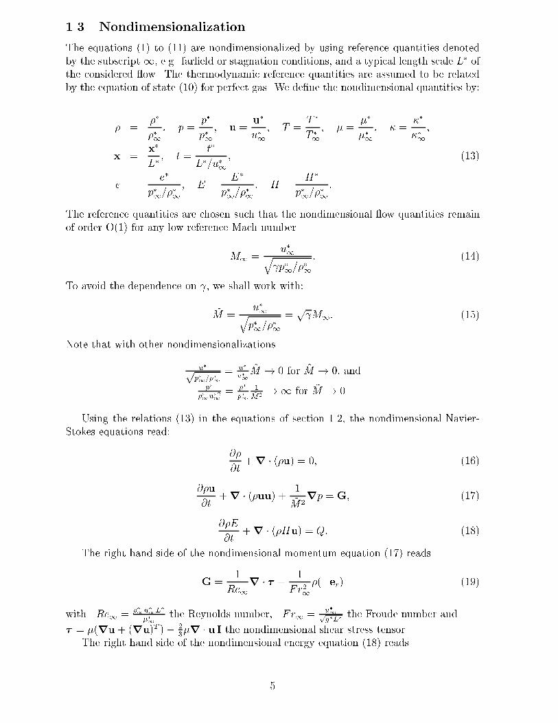
1.3 NondimensionalizationThe equations (1) to (11) are nondimensionalized by using reference quantities denotedby the subscript1, e.g. far�eld or stagnation conditions, and a typical length scale L� ofthe considered ow. The thermodynamic reference quantities are assumed to be relatedby the equation of state (10) for perfect gas. We de�ne the nondimensional quantities by:� = ����1 ; p = p�p�1 ; u = u�u�1 ; T = T �T �1 ; � = ����1 ; � = ����1 ;x = x�L� ; t = t�L�=u�1 ; (13)e = e�p�1=��1 ; E = E�p�1=��1 ; H = H�p�1=��1 :The reference quantities are chosen such that the nondimensional ow quantities remainof order O(1) for any low reference Mach numberM1 = u�1q p�1=��1 : (14)To avoid the dependence on , we shall work with:~M = u�1qp�1=��1 = p M1: (15)Note that with other nondimensionalizationsu�pp�1=��1 = u�u�1 ~M ! 0 for ~M ! 0, andp���1u�21 = p�p�1 1~M2 !1 for ~M ! 0.Using the relations (13) in the equations of section 1.2, the nondimensional Navier-Stokes equations read: @�@t +r � (�u) = 0; (16)@�u@t +r � (�uu) + 1~M2rp = G; (17)@�E@t +r � (�Hu) = Q: (18)The right hand side of the nondimensional momentum equation (17) readsG = 1Re1r � � + 1Fr21�(�er) (19)with Re1 = ��1u�1L���1 the Reynolds number, Fr1 = u�1pg�L� the Froude number and� = �(ru+ (ru)T )� 23�r � u I the nondimensional shear stress tensor.The right hand side of the nondimensional energy equation (18) reads5

Q = ~M2Re1r � (� � u) + ~M2Fr21�(�er) � u + ( � 1)Re1Pr1r � (�rT ) + �q (20)with Pr1 = c�p��1��1 the Prandtl numberand q = q�u�1p�1L���1 the nondimensional heat release rate.The nondimensional expressions of the total energy per unit mass and the total en-thalpy are E = e + ~M2 12 juj2; (21)H = E + p�: (22)The nondimensional equations of state for a perfect gas readp = �T; (23)e = 1 � 1T: (24)Using equations (23), (24) and (21), the pressure can be expressed in terms of the con-servative variables �, �u and �E byp = ( � 1)[�E � ~M2 12 j�uj2� ]: (25)If we assume Pr = c�p���� = Pr1 and c�p = const, we obtain ����1 = ����1 . Then:� = �: (26)The viscosity might for example be determined by the Sutherland law� = T 32 1 + ST + S (27)with S = 110KT �1 for air at standard conditions.1.4 Single Scale Asymptotic AnalysisBefore addressing the numerical solution of the Navier-Stokes equations in part 2, weshall employ perturbation methods [19], [20] to derive approximations of the Navier-Stokes equations at low Mach numbers and to get insight into the underlying physicalmechanisms. The asymptotic analysis allows to identify terms that can be neglected, asa parameter - in our case the reference Mach number or ~M - becomes small. Here, weillustrate the regular perturbation method by deriving the low Mach number equations.We follow the asymptotic analysis by Rehm and Baum [10] for inviscid thermally drivenbuoyant ow and by Majda [6], [17] for low Mach number combustion.We assume that the independent variables are fully characterized by the length scaleL� and the time scale L�=u�1 used to nondimensionalize the space and time variables x�and t� in (13). Thus, we assume that the single time scale variable t and the single space6

scale variable x fully describe the low Mach number ow. Moreover, we assume that thelow Mach number asymptotic analysis is a regular perturbation problem, i.e. all owvariables can be expanded in power series of ~M as for example the pressurep(x; t; ~M) = p0(x; t) + ~Mp1(x; t) + ~M2p2(x; t) +O( ~M3): (28)p0, p1 and p2 are called the zeroth- (or leading), �rst- and second-order pressure, respec-tively.Inserting the asymptotic expansions of �u, � and u into the de�nition of the momentumdensity as density times velocity �u = � u; (29)yields (�u)0 + ~M(�u)1 + ~M2(�u)2 +O( ~M3)= (�0 + ~M�1 + ~M2�2 +O( ~M3)) (u0 + ~Mu1 + ~M2u2 +O( ~M3))= �0u0 + ~M(�0u1 + �1u0) + ~M2(�0u2 + �1u1 + �2u0) +O( ~M3): (30)Ordering the terms in equation (30) according to the powers of ~M leads to the equation[(�u)0��0u0]+[(�u)1�(�0u1+�1u0)] ~M+[(�u)2�(�0u2+�1u1+�2u0)] ~M2+O( ~M3) = 0:(31)Since equation (31) is supposed to hold for arbitrary values of ~M , the coe�cients of themonomials ~M l; l = 0; 1; 2; :::; must be zero. Therefore, we obtain for the zeroth-, �rst-and second-order momentum densities(�u)0 = �0u0; (32)(�u)1 = �0u1 + �1u0; (33)(�u)2 = �0u2 + �1u1 + �2u0: (34)Thus, we can express the zeroth-, �rst- and second-order velocities asu0 = (�u)0=�0; (35)u1 = ((�u)1 � �1u0)=�0; (36)u2 = ((�u)2 � �1u1 � �2u0)=�0: (37)Similarly, we use the relation (25) and the nondimensional equation of state (23) to expressthe pressure and thereby also the temperature in terms of the conservative variables. Theasymptotic expansion yields p0 = ( � 1)(�E)0; (38)p1 = ( � 1)(�E)1; (39)p2 = ( � 1)[(�E)2 � 12�0ju0j2]; (40)T0 = p0�0 ; (41)T1 = p1 � �1T0�0 ; (42)T2 = p2 � �1T1 � �2T0�0 : (43)7

Using the de�nition of the total enthalpy (22) and the equations (38) and (39), theasymptotic expansion yields (�H)0 = � 1p0 (44)and (�H)1 = � 1p1: (45)The asymptotic expansion of �Hu equal �H times u yields(�Hu)0 = (�H)0u0; (46)(�Hu)1 = (�H)0u1 + (�H)1u0: (47)After the asymptotic analysis of the algebraic equations, we shall now consider thepartial di�erential equations. Inserting the asymptotic expansions of the density � andthe momentum density �u into the continuity equation (16) and ordering according topowers of ~M leads to[@�0@t +r � (�u)0] + [@�1@t +r � (�u)1] ~M + [@�2@t +r � (�u)2] ~M2 +O( ~M3) = 0: (48)Requiring the coe�cients of ~M l; l = 0; 1; 2; i.e. the terms in square brackets in (48), tovanish we obtain @�l@t +r � (�u)l = 0; l = 0; 1; 2: (49)For the momentum equation (17), we obtain after inserting the asymptotic expansions ofall ow variables involved and ordering according to the powers of ~Mrp0 ~M�2 +rp1 ~M�1 + @�0u0@t +r � (�0u0u0) +rp2 �G0 +O( ~M) = 0; (50)where G0 = 1Re1r � � 0 + 1Fr21�0(�er) with � 0 = �0(ru0 + (ru0)T )� 23�0r � u0 I .We assume that the Reynolds and Froude numbers are �xed as we vary the Mach number.In equation (50), we require the coe�cients of ~M l; l = �2;�1; 0; to vanish. Thus, we getthe relations rp0 = 0; (51)rp1 = 0; (52)@�0u0@t +r � (�0u0u0) +rp2 = G0: (53)For the energy equation, we proceed similarly as for the continuity equation and obtain@(�E)l@t +r � (�Hu)l = Ql; l = 0; 1; 2; (54)where Ql = ( �1)Re1Pr1r � (�rT )l + (�q)l; l = 0; 1;and Q2 = 1Re1r � (� 0 � u0) + 1Fr21�0(�er) � u0 + ( �1)Re1Pr1r � (�rT )2 + (�q)2 .Equations (51) and (52) derived from the asymptotic analysis of the momentum equationimply that p0 = p0(t) (55)8

and p1 = p1(t); (56)i.e. p0 and p1 are functions of time only. Using equations (38) and (39), we arrive at asimilar conclusion for the zeroth- and �rst-order total energy densities, i.e.(�E)0 = (�E)0(t) (57)and (�E)1 = (�E)1(t): (58)Inserting equations (38), (46), (44) and (39), (47), (45) into the zeroth- and �rst-orderenergy equations (54) for l = 0 and l = 1, respectively, we obtaindp0dt + p0r � u0 = ( � 1)Q0 (59)and dp1dt + p0r � u1 + p1r � u0 = ( � 1)Q1: (60)Using the zeroth-order continuity equation (49), l = 0, and the zeroth-order equation ofstate (41), the zeroth-order energy equation (54), l = 0, can be expressed as � 1�0[@T0@t + u0 �rT0]� dp0dt = Q0: (61)Multiplying the �rst-order Navier-Stokes equations (49), (52), (54), l = 1, by ~M andadding the zeroth-order Navier-Stokes equations (49), (51), (54), l = 0, we obtain thesame equations for ~V0 = V0 + ~MV1 (62)as the zeroth-order Navier-Stokes equations for V0, where V = (�;u; p)T . Thus, we donot win any new information by the �rst-order expansion V1, and we can equally wellstart o� the asymptotic analysis by expansions of the formp(x; t; ~M) = p0(x; t) + ~M2p2(x; t) +O( ~M3) (63)instead of (28).Let us summarize the single scale asymptotic analysis: If a space scale L� and thetime scale L�=u�1, i.e. the time it takes the reference ow to traverse the distance L�,fully describe the considered low Mach number ow, the low Mach number limit yieldsthe zeroth-order Navier-Stokes equations (49), l = 0, (53), (61), i.e.@�0@t +r � (�u)0 = 0; (64)@�0u0@t +r � (�0u0u0) +rp2 = G0: (65) � 1�0[@T0@t + u0 �rT0]� dp0dt = Q0: (66)With (55), the zeroth-order equation of state (41) readsp0(t) = �0(x; t)T0(x; t): (67)9

The zeroth-order Navier-Stokes equations (64), (65), (66), (67) are called low Mach num-ber equations or zero Mach number equations. For combustion, the heat release rate (�q)0depends on chemical reactions and therefore on the involved species densities, which aredetermined by the species continuity equations [17], [21].The zeroth-order pressure p0 can be determined by integrating the zeroth-order energyequation in the form (59) over the volume V of the computational domain [10]dp0dt ZV dV + p0 Z@V u0 � n dA = ( � 1) ZV Q0 dV (68)Knowing the volume ow R@V u0 � ndA and the total heat conduction and heat releaserate RV Q0dV in the computational domain, the ODE (68) can be solved for p0(t) startingfrom an initial condition p0(0).The energy equation (66) is an evolution equation for the temperature T0(x; t). Thedensity �0(x; t) is determined by the equation of state (67). The energy equation in theform (59) implies for the divergence of the velocityr � u0 = � 1 p0 Q0 � 1 p0 dp0dt : (69)Thus, the divergence of u0 is a�ected by the heat conduction and heat release rate Q0and the time change of the zeroth-order pressure p0. Although the divergence of u0 is ingeneral not zero, the roles of the velocity u0 and the second-order pressure p2 are similarto velocity and pressure in incompressible ow. Assuming the density �0 and the righthand side of equation (69), i.e. , p0, dp0dt and Q0, to be known, we may determine u0and p2 similarly as in incompressible ow. For any smooth u0 and �0, the divergence ofthe momentum equation (65) yields a Poisson equation for the second-order pressure p2.At this point, the viscous and buoyancy forces described by G0 come into play. u0 isdetermined by the divergence constraint (69).Of course, the density �0 couples the momentum and energy equations via the equa-tion of state (67). That coupling is more involved than the coupling via the buoyancyterm in the Boussinesq equations, which are only valid for small density and tempera-ture variations [10]. To the contrary, the low Mach number equations (64), (65), (66),(67) admit large density and temperature variations. For small density and temperaturevariations, the Boussinesq equations can be derived from the low Mach number equations[10]. If buoyancy in the Boussinesq equations can be neglected, the energy equation is de-coupled from the momentum and continuity equations, which become the incompressible ow equations [10].The second-order pressure p2 in the low Mach number equations has an importantproperty in common with the pressure in the Boussinesq equations and in the incom-pressible Euler and Navier-Stokes equations: The pressure is decoupled from density andtemperature uctuations arising through the equation of state. Instead, the pressure isdetermined by the constraint on the divergence of velocity. Therefore, acoustic waves areremoved from the low Mach number equations like from the Boussinesq and incompressible ow equations. Consequently, similar methods as for the Boussinesq and incompressible ow equations can be used to solve the low Mach number equations numerically, e.g [17],[21].1.5 Multiple Scales Asymptotic AnalysisThe objective of this section is to give insight into the compressible Navier-Stokes equa-tions at low Mach number, when slow ow is a�ected by acoustic e�ects in a bounded10

region over a long time. We may think of a modern gas turbine combustor, where acousticwaves are re ected at the turbine inlet and the upstream wall and interact many timeswith the turbulent ame [22].

LFigure 1: Piston slowly moving in a cylinder.Another application in mind is a closed piston-cylinder system (Fig. 1), in which theisentropic compression due to a slow piston motion is modi�ed by acoustic waves. Theseare generated by the piston start and propagate back and forth many times, becausethey are re ected at the cylinder end and piston. In that problem, we have one lengthscale, say the initial distance between piston and cylinder end, and two time scales:the long time it takes the slow ow, i.e. the piston, to travel one length scale and theshort time it takes an acoustic wave to travel one length scale. Opposed to a regularlow Mach number expansion, an asymtotic analysis with two time scales and one spacescale together with the analytical method of characteristics avoids secular (i.e. singular)terms and allows G.H. Schneider [23] (cf. W. Schneider [19], pp. 235-240) and Kleinand Peters [24] to account for the cumulative acoustic e�ects in the inert and reactingpiston-cylinder problems, respectively. Using a similar asymptotic approach, Rhadwanand Kassoy [25] investigate the acoustic response due to boundary heating in a con�nedinert gas. Here, the multiple time scale and single space scale asymptotic analysis isemployed to get a better understanding of the low Mach number limit of the compressibleNavier-Stokes equations and to derive simpli�ed equations, which account for the nete�ect of periodic acoustic waves on slow ow over a long time. The present work isbased on the author's habilitation thesis [14] and the article [15]. A general descriptionof multiple scales asymptotic analysis may be found in [19], [26].Since we are interested in slow ow a�ected by acoustic e�ects in a con�ned gas overa long time, we introduce the fast acoustic time scale� �1 = L�qp�1��1 : (70)The acoustic time scale variable is de�ned by� = t�� �1 = t~M (71)The ow and acoustic time scales are illustrated in Figs. 2 and 3 for the two characteristicsdx�dt� = u�1 and dx�dt� = qp�1��1 = c�1p , respectively. Whereas the ow time scale is determined11

by the time it takes the reference ow to travel one length scale, the acoustic time scalecorresponds to the time it takes to travel one length scale at the reference speed of sounddivided by p . In the two time scale, single space scale low Mach number asymptotic

Figure 2: Characteristics in ow time.analysis, each ow variable is expanded as e.g. the pressurep(x; t; ~M) = p0(x; t; �) + ~Mp1(x; t; �) + ~M2p2(x; t; �) +O( ~M3) (72)with � = t~M and ~M = u�1pp�1=��1 .The time derivative at constant x and ~M involves the ow time derivative @@t and theacoustic time derivative @@� :@p@t jx; ~M = ( @@t + 1~M @@� )[p0 + ~Mp1 + ~M2p2 +O( ~M3)] (73)The leading, �rst- and second-order continuity equations read@�0@� = 0; (74)@�1@� + @�0@t +r � (�u)0 = 0; (75)@�2@� + @�1@t +r � (�u)1 = 0: (76)Equation (74) implies that �0 does not depend on the acoustic time scale, i.e. �0 = �0(x; t).The leading, �rst- and second-order momentum equations are derived as12

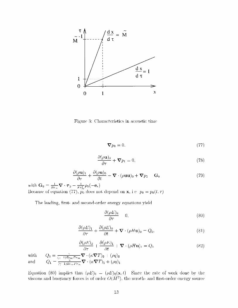
Figure 3: Characteristics in acoustic time.rp0 = 0; (77)@(�u)0@� +rp1 = 0; (78)@(�u)1@� + @(�u)0@t +r � (�uu)0 +rp2 = G0 (79)with G0 = 1Re1r � � 0 + 1Fr21�0(�er)Because of equation (77), p0 does not depend on x, i.e. p0 = p0(t; �).The leading, �rst- and second-order energy equations yield@(�E)0@� = 0; (80)@(�E)1@� + @(�E)0@t +r � (�Hu)0 = Q0; (81)@(�E)2@� + @(�E)1@t +r � (�Hu)1 = Q1 (82)with Q0 = ( �1)Re1Pr1r � (�rT )0 + (�q)0and Q1 = ( �1)Re1Pr1r � (�rT )1 + (�q)1Equation (80) implies that (�E)0 = (�E)0(x; t). Since the rate of work done by theviscous and buoyancy forces is of order O( ~M2), the zeroth- and �rst-order energy source13

terms Q0 and Q1 are governed by heat conduction and heat release rate only, providedthe Prandtl number Pr1 is of order O(1) and the Froude number squared Fr21 is of orderO(Re1Pr1) assuming that the ratio ( �1)= is of order O(1) in both cases. However, ifthe Reynolds number Re1 is of the order O( ~M2), i.e. the reference pressure p�1 is of theorder of the viscous force per unit area O(��1u�1=L�), or if the Froude number Fr1 is ofthe order O( ~M), i.e. the reference pressure p�1 is of the order of the hydrostatic pressureO(��1g�L�), then the rate of work done by the viscous or buoyancy forces, respectively,will also contribute to the zeroth-order energy source term Q0.For the algebraic equations, the asymptotic expansion yields the same relations as forthe single scale asymptotic analysis (32) - 47).Using the consequences of equations (77) and (80) in (38), we obtain for the zeroth-order pressure p0(t; �) = ( � 1)(�E)0(x; t): (83)Consequently, the zeroth-order pressure p0 and the zeroth-order total energy density (�E)0only depend on the ow time t, and we getp0(t) = ( � 1)(�E)0(t): (84)Using the consequence of equation (74), the �rst-order momentum equation (78) canbe simpli�ed to @u0@� + 1�0rp1 = 0: (85)With �0H0 = (�E)0 + p0 = �1p0, (38), and (39), the �rst-order energy equation (81)becomes @p1@� + p0r � u0 = ( � 1)Q0 � dp0dt : (86)Subtracting the divergence of (85) multiplied by p0 from the acoustic time derivativeof (86), i.e. @@� (86) � p0r� (85), yields (since @@� and r� commute)@2p1@� 2 �r � (c20rp1) = ( � 1)@(�q)0@� : (87)Note that c20 = p0(t)�0(x;t) depends on x and t, but not on � . Thus, (87) represents aninhomogeneous linear wave equation with nonconstant coe�cient c20. Its source is dueto the acoustic time change of the zeroth-order heat release rate. The source of (87)is not a�ected by heat conduction, because the acoustic time derivative of the zeroth-order temperature T0 = p0(t)=�0(x; t) vanishes. The rate of work done by the viscousand buoyancy forces does not a�ect the �rst-order pressure p1, unless the conditionsRe1 = O( ~M2) or Fr1 = O( ~M), respectively, hold.If the zeroth-order speed of sound c0 is approximated by the ambient speed of soundc1 (with the ambient chosen as reference state), equation (87) constitutes the basic equa-tion of thermoacoustics to describe acoustic e�ects in combustion [27], [28]. The acoustictime change of the heat release rate constitutes the dominant thermoacoustic source incombustion, as the right hand side of (87) is governed by the monopole source ( �1)@(�q)0@�[27], [28]. The governing equation of thermoacoustics, i.e. the simpli�cation of (87) just14

mentioned, can also be derived by simplifying Lighthill's acoustic analogy for combustion[27]. That equation can be solved analytically by means of Green's function [29].The zeroth-order pressure p0 can be determined by integrating equation (86) over thevolume V of the computational domain as for the low Mach number equations [10]:dp0dt ZV dV + p0 Z@V u0 � ndA = ( � 1) ZV Q0dV � ZV @p1@� dV: (88)Knowing u0 at the boundary of the computational domain or just the volume ow, know-ing the heat conduction and heat release rate RV Q0dV in the computational domain andassuming that the integrated e�ect of the acoustic time change of the �rst-order pressureis negligible, i.e. RV @p1@� dV = 0, the ODE (88) can be solved for p0(t) starting from aninitial condition p0(0) as equation (68) for the low Mach number equations.Equation (86), derived from the �rst-order energy equation, has an interesting conse-quence for the divergence of the zeroth-order velocity:r � u0 = � 1 p0 Q0 � 1 p0 [dp0dt + @p1@� ]: (89)Thus, the divergence of u0 is a�ected by the heat conduction and heat release rate Q0,the time change of the global pressure p0 and the acoustic time change of the �rst-orderpressure p1.Using the product rule in the �rst-order continuity equation (75) and inserting (89),the zeroth-order density change along the zeroth-order path line reads@�0@t + u0 �r�0 = � � 1c20 Q0 + 1c20 dp0dt + @@� (p1c20 � �1): (90)Thus, the zeroth-order density of a uid particle is changed by the heat conduction andheat release rate Q0, the global pressure time change dp0dt and by the acoustic time changeof the �rst-order entropy, i.e. @@� (p1c20 � �1).1.6 Removal of Acoustics and Signi�cance of PressureIn this section, we discuss the removal of acoustics and the signi�cance of the pressurein low Mach number ow. If the �rst-order continuity and energy equations and thesecond-order momentum equation of the previous multiple scales asymptotic analysis areaveraged over an acoustic wave period, the averaged velocity tensor describes the netacoustic e�ect on the averaged ow �eld. Removing acoustics altogether leads to the lowMach number equations. The physical signi�cance of the zeroth-, �rst- and second-orderpressures is discussed.We assume acoustic waves with period Ta such that (�1; (�u)1; (�E)1)T (x; t; �) =(�1; (�u)1; (�E)1)T (x; t; � +Ta). Integrating equation (90) over a period Ta of the acousticwave using R Ta0 @@� (p1c20 � �1)d� = 0, we obtain the simpli�cation@�0@t + �u0 �r�0 = � � 1c20 �Q0 + 1c20 dp0dt : (91)where the overbar denotes acoustic time averaging, i.e. �u0(x; t) = 1Ta R Ta0 u0(x; t; �)d� forthe averaged velocity. 15

Similarly, equation (89) can be simpli�ed by integration:r � �u0 = � 1 p0 �Q0 � 1 p0 dp0dt : (92)Integrating the second-order momentum equation (79) over the acoustic wave periodTa, we get @�0�u0@t +r � (�0u0u0) +r�p2 = �G0; (93)where the averaged velocity tensor u0u0 = 1Ta R Ta0 u0(x; t; �)u0(x; t; �)d� describes thenet acoustic e�ect on the averaged ow �eld. The solution of the averaged momen-tum equation (93) requires the knowlege of u0(x; t; �) over an acoustic wave periodto determine u0u0. In a numerical solution, we might be able to choose the numer-ical time step �t equal to the acoustic wave period Ta and solve the inhomogeneouswave equation (87) by subdividing Ta into a number of acoustic time steps �� to ob-tain p1(x; t; � + m��); m = 1; :::; Ta=�� . Then, the numerical solution of (85) yieldsu0(x; t; � +m��); m = 1; :::; Ta=�� . Finally, the averaged velocity tensor u0u0 can beobtained by numerical integration.If the averaged velocity tensor u0u0 is approximated by the tensor �u0�u0 of the averagedvelocities, even the net acoustic e�ect is removed from (93) and we obtain the momentumequation in the zero Mach number limit:@�0�u0@t +r � (�0�u0�u0) +r�p2 = �G0: (94)The averaged �rst-order continuity equation (75) yields@�0@t +r � (�0�u0) = 0: (95)Using (95) to express r � �u0 and using the equation of state p0(t) = �0(x; t)T0(x; t),the energy equation (92) becomes � 1�0[@T0@t + �u0 �rT0]� dp0dt = �Q0: (96)Equations (95), (94), (96) coincide with the low Mach number equations (64), (65),(66) derived by the single scale asymptotic analysis in section 1.4.Contrary to the low Mach number equations, the intermediate equations (95), (93),(96) take the acoustic e�ect of the nonlinearity on the averaged ow in the momentumequation into account. It will be interesting to investigate the signi�cance of (93) insteadof (94), because like the low Mach number equations the intermediate equations (95),(93), (96) can be solved more easily than the compressible Navier-Stokes equations.Since the zeroth-order pressure p0(t) serves as the mean pressure in the energy equa-tion, it represents the global thermodynamic pressure part. As the second-order pressurep2(x; t) is determined by the momentum equation as the pressure complying with theconstraint (92) on the velocity divergence analogously to incompressible ow, ~M2p2(x; t)may be called the 'incompressible' pressure part. The low Mach number momentumequation (94) is coupled to the low Mach number energy equation (96) via the density�0, viscosity �(T0) and equation of state p0 = �0T0, whereas the �rst-order momentumand energy equations with acoustics included (85) and (86) are directly coupled by the16

�rst-order pressure p1(x; t; �). Since p1(x; t; �) is governed by the inhomogeneous waveequation (87), ~Mp1(x; t; �) can be identi�ed as the acoustic pressure part. These rolesof the pressure are also identi�ed by a single time scale, multiple space scale low Machnumber asymptotics for the Euler equations [13]. In that analysis, long wave acousticsis described by a homogeneous wave equation for the �rst-order pressure after volumeaveraging the small ow scales.Summarizing the multiple scales low Mach number asymptotic analysis, the pressurep can be split into the sum of� p0(t), the large global thermodynamic pressure,� ~Mp1(x; t; �), the small acoustic pressure,� ~M2p2(x; t; �), the very small 'incompressible' pressure,and higher order terms of O( ~M3).2 Numerical ImplicationsIn section 2.1, the low Mach number asymptotics is used to recommend which equationsto choose for modelling low Mach number ow. After discussing physical and numericalissues of computing low speed ow in section 2.2, numerical methods for low Mach num-ber ow simulations are reviewed in section 2.3. In section 2.4, the perturbation formof the Navier-Stokes equations is introduced to avoid the cancellation problem in lowMach number ow computations. The characteristic based approximate Riemann solverexplained in section 2.5 yields a simple ux evaluation and can be formulated withoutcancellation problems.2.1 Choice of EquationsThe low Mach number asymptotics of the Navier-Stokes equations gives a basic guidancewhich equations to choose for the numerical simulation of low Mach number ow. Theasymptotic analysis shows that acoustic waves are inherent in the Navier-Stokes equationsat low Mach numbers. Acoustics can be �ltered out of the Navier-Stokes equations leadingto the low Mach number equations. Alternatively, acoustics can be �ltered out of theinitial conditions such that the acoustic waves are not excited when solving the Navier-Stokes equations [30].If we are interested in aeroacoustics, Lighthill's acoustic analogy gives insight into thesound generation by ow [29]. Lighthill's equation is the inhomogeneous wave equationfor the acoustic density ��0 = �� � ��o@2��0@t�2 � c�2o ����0 =r� �r� �T�; (97)which is derived without approximation from the continuity and momentum equations.The subscript o denotes the values in the undisturbed uid. The source of (97) is aquadrupole, the strength of which is Lighthill's stress tensor T� with the componentsT �ij = ��u�iu�j + (p�0 � c�2o ��0)�ij � � �ij; (98)17

where p�0 = p� � p�o is the acoustic pressure and � �ij is the viscous stress. The Kroneckerdelta is de�ned by �ij = 1, if i = j and �ij = 0, if i 6= j. T� describes the sound generationdue to ow nonlinearities. The sound propagation in the far�eld is governed by the linearwave equation, because T �ij = const there. Thus, Lighthill's equation (97) shows that thesound generation in ow is due to nonlinearities, whereas the sound propagation is ingeneral linear. If we assume that the acoustic �eld does not a�ect the ow from whichthe sound originated, we can determine the source of sound and compute the acousticdensity as if it were generated by that source in a uid at rest. That approach is calledthe acoustic analogy [31], [32].When the acoustic analogy is used, the incompressible Navier-Stokes equations areusually solved by a suitable CFD method in a small domain V , which contains the sourcesof sound. Having determined Lighthill's stress tensor (98), the analytical solution ofLighthill's equation (97)��0(x�; t�) = 14�(c�0)2r� �r� � ZV T�(y�; t� � jx� � y�j=c�0)jx� � y�j dV (y�): (99)can be evaluated numerically.Using Kirchho�'s theorem, the volume integral in (99) can be expressed as a surfaceintegral. If the acoustic pressure and normal velocity is known on the boundary of V ,that surface integral can be evaluated to determine the acoustic density in the far�eld.The acoustic pressure follows from the isentropic relation p�0 = (c�0)2��0.For aeroacoustic applications, the compressible Navier-Stokes and Euler equations,the linearized Euler equations and the wave equation require highly accurate numericalmethods to compute the acoustic waves accurately and e�ciently [33].With the arguments on low Mach number asymptotics and on basic concepts of com-putational aeroacoustics [34], [35], [36], [33], we arrive at the following recommendations:1. If you are not interested in acoustic e�ects in low Mach number ow, you may usethe(a) low Mach number equations for combustion,(b) Boussinesq equations for free convection,(c) incompressible Navier-Stokes equations for constant density ows and the de-coupled energy equation for forced convection.2. If you are not interested in viscous e�ects in low Mach number ow, you may usethe(a) Euler equations for nonlinear e�ects including inviscid sound generation andsound propagation,(b) potential equation for steady, irrotational and either isentropic or incompress-ible ow,(c) wave equation for linear acoustic e�ects in a uid at rest.3. If you are only interested in acoustic e�ects in low Mach number ow, you may usethe(a) Navier-Stokes equations for nonlinear generation and propagation of sound aswell as resonance, 18

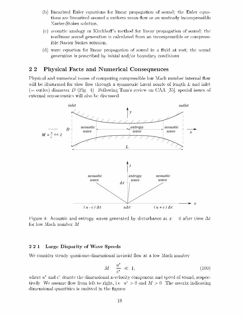
(b) linearized Euler equations for linear propagation of sound; the Euler equa-tions are linearized around a uniform mean ow or an unsteady incompressibleNavier-Stokes solution,(c) acoustic analogy or Kirchho�'s method for linear propagation of sound; thenonlinear sound generation is calculated from an incompressible or compress-ible Navier-Stokes solution,(d) wave equation for linear propagation of sound in a uid at rest; the soundgeneration is prescribed by initial and/or boundary conditions.2.2 Physical Facts and Numerical ConsequencesPhysical and numerical issues of computing compressible low Mach number internal owwill be illustrated for slow ow through a symmetric Laval nozzle of length L and inlet(= outlet) diameter D (Fig. 4). Following Tam's review on CAA [35], special issues ofexternal aeroacoustics will also be discussed.

t

acoustic wave

acoustic wave

entropy wave

L

D

inlet

acoustic wave

outlet

y

entropy wave

acoustic wave

M =

u

c<< 1

x

x( u - c ) ∆ t u∆ t ( u + c ) ∆ t

∆ t

∗

Figure 4: Acoustic and entropy waves generated by disturbance at x = 0 after time �tfor low Mach number M .2.2.1 Large Disparity of Wave SpeedsWe consider steady quasi-one-dimensional inviscid ow at a low Mach numberM = u�c� � 1; (100)where u� and c� denote the dimensional x-velocity component and speed of sound, respec-tively. We assume ow from left to right, i.e. u� > 0 and M > 0. The asterix indicatingdimensional quantities is omitted in the �gures.19

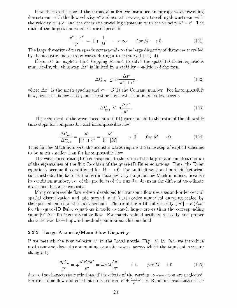
If we disturb the ow at the throat x� = 0m, we introduce an entropy wave travellingdownstream with the ow velocity u� and acoustic waves, one travelling downstream withthe velocity u� + c� and the other one travelling upstream with the velocity u� � c�. Theratio of the largest and smallest wave speeds isu� + c�u� = 1 + 1M �! 1 for M �! 0: (101)The large disparity of wave speeds corresponds to the large disparity of distances travelledby the acoustic and entropy waves during a time interval (Fig. 4).If we use an explicit time stepping scheme to solve the quasi-1D Euler equationsnumerically, the time step �t� is limited by a stability condition of the form�t�com � � �x�ju�j+ c� ; (102)where �x� is the mesh spacing and � = O(1) the Courant number. For incompressible ow, acoustics is neglected, and the time step restriction is much less severe:�t�inc � ��x�ju�j : (103)The reciprocal of the wave speed ratio (101) corresponds to the ratio of the allowabletime steps for compressible and incompressible ow�t�com�t�inc = ju�jju�j+ c� = jM j1 + jM j �! 0 for M �! 0: (104)Thus for low Mach numbers, the acoustic waves require the time step of explicit schemesto be much smaller than for incompressible ow.The wave speed ratio (101) corresponds to the ratio of the largest and smallest moduliof the eigenvalues of the ux Jacobian of the quasi-1D Euler equations. Thus, the Eulerequations become ill-conditioned for M �! 0. For multi-dimensional implicit factoriza-tion methods, the factorization error becomes very large for low Mach numbers, becauseits condition number, i.e. of the products of the ux Jacobians in the di�erent coordinatedirections, becomes excessive.Many compressible ow solvers developed for transonic ow use a second-order centralspatial discretization and add second- and fourth-order numerical damping scaled bythe spectral radius of the ux Jacobian. The resulting arti�cial viscosity (ju�j + c�)�x�for the quasi-1D Euler equations introduces much larger errors than the correspondingvalue ju�j�x� for incompressible ow. For matrix valued arti�cial viscosity and propercharacteristic based upwind methods, similar conclusions hold.2.2.2 Large Acoustic/Mean Flow DisparityIf we perturb the ow velocity u� in the Laval nozzle (Fig. 4) by �u�, we introduceupstream and downstream running acoustic waves, across which the transient pressurechanges by �p�trap� = ���c��u�p� = � M �u�u� �! 0 for M �! 0 (105)due to the characteristic relations, if the e�ects of the varying cross-section are neglected.For isentropic ow and constant cross-section, c� � �12 u� are Riemann invariants on the20

characteristics dx�dt� = u� � c�. Thus, for entropy s� = const, we obtain the transienttemperature change in 1D ow of perfect gas�T �traT � = �c�2c�2 = �( � 1)c��u�c�2 = �( � 1)M�u�u� �! 0 for M �! 0: (106)Using the equation of state (10) for perfect gas, we obtain the transient density change���tra�� = �M �u�u� �! 0 for M �! 0: (107)

Figure 5: Sound generation by a low Mach number jet.Let us consider the example of subsonic jet noise (Fig. 5 after [31]). Depending on thejet velocity, 120dB or even higher sound pressure levels can be measured in the far�eldof the jet at about 50 jet diameters distance. That noise level corresponds to an acous-tic pressure of p�0 = 20Pa. The ratio of acoustic to mean ow pressure p� � 105 Pa isO(10�4).Assuming steady ow, the pressure, temperature and density changes induced by avelocity change �u� are even smaller. Since the total enthalpy H� = c�2 �1 + 12u�2 andentropy s� are constant in steady quasi-1D inviscid ow without shocks, the Bernoulliequation yields the steady pressure change�p�step� = ���u��u�p� = � M2 �u�u� �! 0 for M �! 0: (108)The steady temperature change is derived from H� = const�T �steT � = �c�2c�2 = �( � 1)u��u�c�2 = �( � 1)M2 �u�u� �! 0 for M �! 0: (109)With (10), the steady density change becomes21

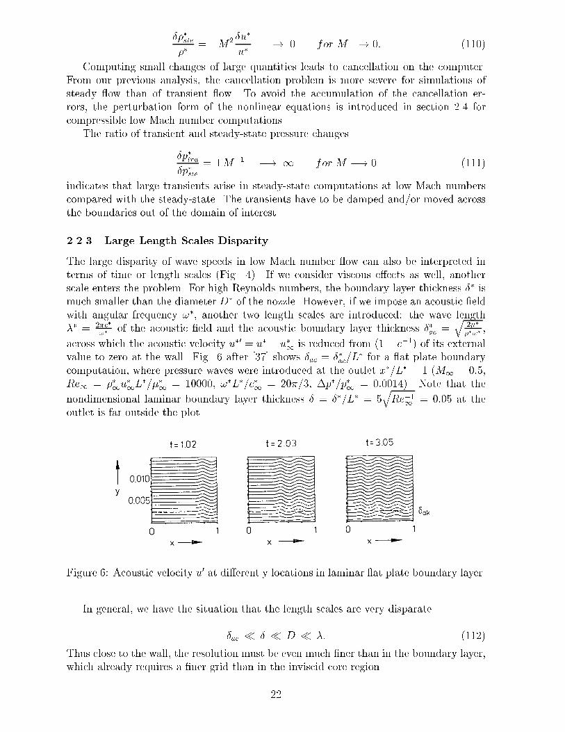
���ste�� = �M2 �u�u� �! 0 for M �! 0: (110)Computing small changes of large quantities leads to cancellation on the computer.From our previous analysis, the cancellation problem is more severe for simulations ofsteady ow than of transient ow. To avoid the accumulation of the cancellation er-rors, the perturbation form of the nonlinear equations is introduced in section 2.4 forcompressible low Mach number computations.The ratio of transient and steady-state pressure changes�p�tra�p�ste = �M�1 �! 1 for M �! 0 (111)indicates that large transients arise in steady-state computations at low Mach numberscompared with the steady-state. The transients have to be damped and/or moved acrossthe boundaries out of the domain of interest.2.2.3 Large Length Scales DisparityThe large disparity of wave speeds in low Mach number ow can also be interpreted interms of time or length scales (Fig. 4). If we consider viscous e�ects as well, anotherscale enters the problem. For high Reynolds numbers, the boundary layer thickness �� ismuch smaller than the diameter D� of the nozzle. However, if we impose an acoustic �eldwith angular frequency !�, another two length scales are introduced: the wave length�� = 2�c�!� of the acoustic �eld and the acoustic boundary layer thickness ��ac = q 2����!� ,across which the acoustic velocity u�0 = u� � u�1 is reduced from (1� e�1) of its externalvalue to zero at the wall. Fig. 6 after [37] shows �ac = ��ac=L� for a at plate boundarycomputation, where pressure waves were introduced at the outlet x�=L� = 1 (M1 = 0:5,Re1 = ��1u�1L�=��1 = 10000, !�L�=c�1 = 20�=3, �p�=p�1 = 0:0014). Note that thenondimensional laminar boundary layer thickness � = ��=L� = 5qRe�11 = 0:05 at theoutlet is far outside the plot.

Figure 6: Acoustic velocity u0 at di�erent y locations in laminar at plate boundary layer.In general, we have the situation that the length scales are very disparate�ac � � � D � �: (112)Thus close to the wall, the resolution must be even much �ner than in the boundary layer,which already requires a �ner grid than in the inviscid core region.22

Broadband turbulent mixing noise is observed in the far�eld of external ow. Forexample in the far�eld of a subsonic turbulent jet, the frequency spans over two decadesfrom f �min � 300Hz to f �max � 30000Hz [38]. Since the highest frequency f �max correspondsto the shortest wave length ��min = c�of�max of the sound waves,f �max determines the spatialresolution requirements. In the experiment of [38], ��min � 0:01m � 14D� where D� is thenozzle exit diameter.Suppose N� points su�ce to resolve one wave length with an error of � and we woulduse an isotropic grid point distribution in a (100D)3 computational box, we would need(100 � 4 � N�)3 grid points to resolve the highest frequency of the sound waves in thefar�eld (not counting the additional points to properly resolve the nonlinear near�eld).As N0:1 = 5 for a sixth order central �nite di�erence method [39], we would need 8 billiongrid points. Even for Lele's spectral-like compact scheme with N0:001 = 2:5 [40], thenumber of grid points to resolve the far�eld sound is excessive. However, since the far�eldacoustic �eld is governed by the linear wave equation, more e�cient methods are availableto compute the far�eld noise than direct numerical simulation.As mentioned in section 2.1, Lighthill's acoustic analogy can be used to determine thefar�eld acoustic density by the exact solution (99) of the inhomogeneous wave equation(97). We have to calculate the volume integral of the quadrupole source of (97) evaluatedat the retarded time when the sound was generated and divided by the distance betweenlistener and source [29]. Approximations thereof for low Mach numbers, e.g. by M�ohring[41], [42], are reviewed by Crighton [2]. The volume integral can be expressed as a surfaceintegral using Kirchho�'s theorem [31]. Applications of the resulting Kirchho� methodin CAA are reviewed by Lyrintzis [34].To predict the directivity and spectrum of the radiated sound in the far�eld, the com-puted solution must be accurate throughout the entire computational domain. Thus, theaccuracy requirements are much more severe then in conventional CFD, where usuallyonly in the vicinity of the aerodynamic body accuracy is required. As the travelling dis-tance from the sound source to the far�eld is quite long ( � 100 nozzle diameters for jetnoise (Fig. 5) is realistic), the acoustic waves have to be accurately computed over a longpropagation distance by direct numerical simulation. Thus, the numerical dispersion anddissipation errors have to be kept low from the near�eld to the far�eld when using directnumerical simulation or up to a surface, beyond which the sound propagation is gov-erned by the linear wave equation, when using Lighthill's acoustic analogy or Kirchho�'smethod.2.2.4 Boundary ConditionsAt arti�cial boundaries, i.e. in ow, out ow and far�eld, the boundary conditions shouldallow the acoustic waves travelling at the velocity u� + c�n in any direction n and theentropy and vorticity waves travelling at the ow velocity u� to leave the computationaldomain with minimal re ection in order to mimic an in�nite domain. Otherwise there ections will corrupt the results. In the inviscid ow regions, the non-re ecting boundaryconditions developed for the Euler equations can be used [43], [44], [45], [46], [47], [48],[49],[50], pp. 387-395, [51],[52], [53], [54], [55], [14]. For the Navier-Stokes equations moreinformation is required at the arti�cial boundaries than for the Euler equations [56], [57],[58], [59], [60], [61], [62].For low Mach number ow, the acoustic waves travel aboutM�1 times faster than theentropy and vorticity waves. Therefore, any re ected wave will very quickly corrupt the23

entire ow �eld. Thus, the proper boundary treatment of the acoustic waves is particularlyimportant for low Mach number ow.The signi�cance of non-re ecting boundary conditions for the accuracy of unsteady ow and the convergence of steady ow was demonstrated by M�uller [55], [14] for internal ow. Prescribing the pressure p = pambient at the outlet leads to complete re ection ofan acoustic wave, i.e. a right going acoustic wave is re ected at the outlet boundary asa left going acoustic wave with the same amplitude. Prescribing the entropy s = s0 atthe inlet corresponds to a non-re ecting boundary condition for the entropy wave, i.e.@p@t � c2 @�@t = 0 at the inlet, cf. (139). However, prescribing the total enthalpy H = H0leads to almost complete re ection of an acoustic wave, i.e. a left going acoustic wave isre ected at the inlet boundary as a right going acoustic wave with the amplitude reducedby the factor 1�M1+M [55], [14]. For low Mach numbers M , that factor is close to 1, i.e.close to complete re ection. The re ection of the acoustic waves at outlet and inlet inlow Mach number ow is sketched in the x-t-diagram in Fig. 7. Even after the entropywave has left the outlet without re ection, the acoustic waves continue to bounce backand forth. Their amplitude is only slightly reduced at the inlet.t t

xFigure 7: Re ection of acoustic waves at outlet and inlet in low Mach number ow.These �ndings are con�rmed by the computation of an acoustic pulse in a 1D tubeusing the Euler equations. The Mach number of the initially uniform ow is M0 = 10�2.24

A pressure pulse is imposed at the outlet x� = L� during 0 � t� � t�p as in [63]:p�(L�; t�) = p�0(1 + � sin4(�t�=t�p)) (113)with t�p = 13 L�c�0�u�0 and � = 10�2. 241 equidistant grid points are used. The time stepof �t�L�=c�0 = 1:25 � 10�3 corresponds to a maximum Courant number of 0:303. Fig. 8shows the acoustic pressure at six time instants when using the re ecting inlet boundaryconditions mentioned above. At � = t�L�=c�0 = 1, the acoustic pulse (cf. solid line in plot)has travelled from the outlet close to the inlet. At � = 1:1, the shape of the acoustic waveis altered by the re ecting boundary conditions. At � = 1:2, the acoustic pressure haschanged sign. For � = 1:3; 1:4 and 1:5, we observe the re ected acoustic wave travellingtowards the outlet.

Figure 8: Acoustic pressure for acoustic pulse re ected at the inlet computed with re ect-ing boundary conditions.The non-re ecting boundary conditions require the incoming characteristic variablesnot to change and the outgoing ones to be determined from the interior [43]. With non-re ecting boundary conditions, the inlet becomes permeable for the acoustic wave. Ittraverses the inlet with almost no re ection, as Fig. 9 illustrates. The acoustic pressureafter � = 1:4 is almost zero. Actually, it is about 5 orders of magnitude lower than withre ecing boundary conditions.For steady low Mach number ow, non-re ecting boundary conditions are decisivefor the convergence, because with re ecting boundary conditions the acoustic waves arere ected at inlet and outlet and only reduced due to viscosity and a small reduction wheninteracting with the inlet for H = H0. We consider the quasi-1D inviscid ow in a Lavalnozzle with the cross-sectional area 25

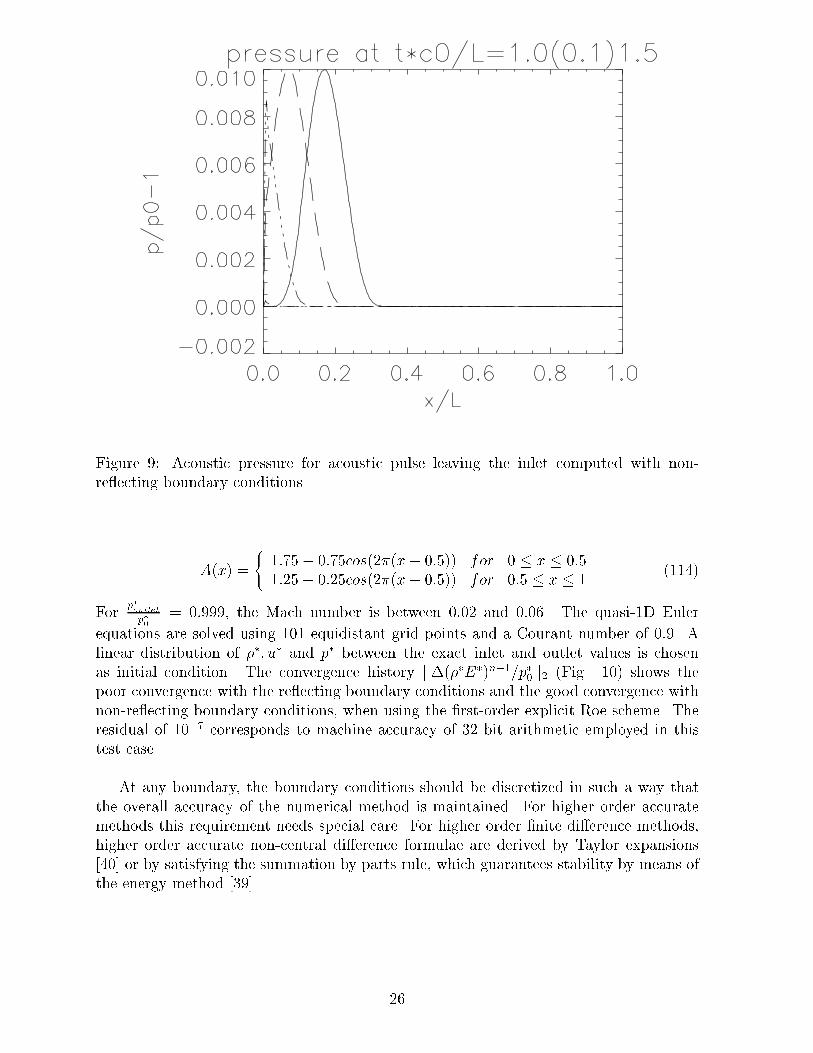
Figure 9: Acoustic pressure for acoustic pulse leaving the inlet computed with non-re ecting boundary conditions.A(x) = ( 1:75� 0:75cos(2�(x� 0:5)) for 0 � x � 0:51:25� 0:25cos(2�(x� 0:5)) for 0:5 � x � 1 (114)For p�outletp�0 = 0:999, the Mach number is between 0:02 and 0:06. The quasi-1D Eulerequations are solved using 101 equidistant grid points and a Courant number of 0:9. Alinear distribution of ��; u� and p� between the exact inlet and outlet values is chosenas initial condition. The convergence history jj�(��E�)n�1=p�0jj2 (Fig. 10) shows thepoor convergence with the re ecting boundary conditions and the good convergence withnon-re ecting boundary conditions, when using the �rst-order explicit Roe scheme. Theresidual of 10�7 corresponds to machine accuracy of 32 bit arithmetic employed in thistest case.At any boundary, the boundary conditions should be discretized in such a way thatthe overall accuracy of the numerical method is maintained. For higher order accuratemethods this requirement needs special care. For higher order �nite di�erence methods,higher order accurate non-central di�erence formulae are derived by Taylor expansions[40] or by satisfying the summation by parts rule, which guarantees stability by means ofthe energy method [39].

26

-8

-7.5

-7

-6.5

-6

-5.5

-5

-4.5

-4

-3.5

-3

0 1000 2000 3000 4000 5000 6000 7000 8000 900010000

log|

|ene

rgy

flux

dif

fere

nce|

|_2

n

1st order explicit Roe, CFL=0.9

reflecting b.c.non-reflecting b.c.

Figure 10: Convergence history for Laval nozzle (0:02 < M < 0:06).2.3 Literature ReviewExcellent introductions to aeroacoustics are provided by Lighthill [64], Dowling and FfowcsWilliams [31], Landau and Lifshitz [65], chapter 8, and others. Acoustics in a broadersense is treated e.g. by Pierce [66]. Brief reviews on the emerging �eld of computationalaeroacoustics are given by [35] and [67], chapter 9. The proceedings of a recent workshopon CAA [68] may serve as an introduction.In the direct numerical simulation of aerodynamic noise, central �nite di�erence dis-cretizations are preferred, because they avoid dissipation errors [69]. Since higher orderdi�erence approximations are more e�cient than the conventional second-order centralscheme to compute wave propagation (cf. e.g. [39], chapter 3), the former are favouredin CAA [35]. As mentioned in section 2.2.3, even more accurate compact �nite-di�erencemethods with fourth-order formal accuracy but spectral-like resolution were devised [40].The dispersion error can be further minimized for long time integration by taking theinitial values into account [70]. Explicit Runge-Kutta and Adams-Bashforth methods areoptimized to keep the dissipation and dispersion errors due to time integration low [71],[54]. Thomas and Roe [72] devised an upwind variant of the leapfrog scheme, which is non-dissipative and has low dispersion error. In multi dimensions, �nite di�erence methodsintroduce anisotropy errors, because for example in 2D the numerical phase velocity in thedirections m�=4, m odd, is larger and more accurate than in the directions m�=4, m even[73], chapter 10. Averaging the di�erence operators in the transverse directions helps toreduce the anisotropy error at the expense of a wider stencil [73]. Streng, Kuerten, Broeze,and Geurts [74] developed a fourth-order accurate di�erence method of that kind for thedirect numerical simulation of compressible ow. In order to avoid numerical contamina-tion by the unresolved waves with very short wave lengths, these waves and only these27

should be damped by added higher order numerical damping for central discretizations[39], [35] or by using higher order upwind discretizations.Besides the explicit higher order di�erence methods developed for the direct numericalsimulation of aeroacoustics, there are also other techniques usually developed for e�cientsecond-order accurate computations of steady and/or unsteady low Mach number compu-tations. Often, the density-based 'compressible' methods have originally been developedfor transonic ow simulations and lately been applied to low Mach number ow [3]. Thepressure-based 'incompressible' techniques have recently been extended from incompress-ible to compressible ow [75], [76], [77], [78], [79], [80], [81], [82]. According to [83], thesimultaneous solution of the conservation laws in 'compressible' methods enhances stabil-ity compared with the sequential solution approach of 'incompressible' techniques, whichemploy a Poisson equation for the pressure instead of the continuity equation. Here, weshall focus on 'compressible' methods.Time derivative preconditioning can be used to accelerate the convergence to steady-state for low Mach numbers , because the condition number of the modi�ed inviscidsystem is brought close to 1 instead of M�1 for the Euler equations, e.g. [84]. Since thenumerical damping added to central discretizations and inherent in upwind schemes scaleswith the condition number, the associated numerical damping error is much lower with thepreconditioned system than with the original one for small M . The improved conditionnumber allows more e�cient applications of implicit methods, e.g. [85], [86], [87]. As theeigenvalues of the modi�ed system are brought close to each other compared with theoriginal disparity, smoothing of all waves and not just the fastest ones renders multigridmethods more e�cient for the preconditioned system than for the original one, e.g. [88],[89], [90]. Using dual time stepping for unsteady ow simulation, the preconditionedsystem is iterated to steady-state in pseudo-time for each physical time step using astrongly implicit technique by [91]. Eriksson devised a preconditioning for low speedcombustion [92]. For viscous ow, Choi and Merkle also take the cell Reynolds number�u4x� into account [93], [94]. An excellent review on matrix and di�erential preconditioningis given by Turkel [95]. The recent developments are addressed by other lecturers at this\30th Computational Fluid Dynamics" VKI Lecture Series.Implicit methods and multigrid methods yield convergence acceleration even withoutpreconditioning. Using Jameson's multigrid �nite volume method with residual smoothingand Pulliam and Steger's implicit �nite di�erence method based on approximate factoriza-tion, Volpe was able to compute steady ow over a circular cylinder atM1 = 0:1; 0:01, and0:001 [3]. However, accuracy and convergence problems were encountered for M1 �! 0.Similar conclusions were drawn from quasi-1D inviscid Laval nozzle computations at lowMach numbers, when using an implicit upwind scheme [96], [97] and a multigrid acceler-ation of an explicit upwind scheme [98]. Implicit methods can also be used for unsteady ow computations at low Mach numbers. For example, Chen and Pletcher [99] computeunsteady ow over a circular cylinder with a strongly implicit procedure formulated forp;u, and T .Semi-implicit methods have mainly been devised for unsteady ow simulations. Gustafs-son and co-workers use the new variable � = 2 �1 c��c�1u�1 to symmetrize the isentropic Eu-ler and Navier-Stokes equations, which reduce to the incompressible ow equations forM1 ! 0 [100], [101], [102]. The resulting symmetric system is solved by a semi-implicitcentral di�erence scheme: the terms of O(M�11 ) are discretized in time by the implicitEuler method, while the leapfrog scheme or an explicit one-step method is used for the28

other terms of O(1). Casulli and Greenspan [103] and Patnaik et al. [104] have shown thatonly the pressure and velocity terms in the momentum and energy equations, respectively,have to be treated implicitly to remove the sound speed restriction on the time step (102).Thus, the implicit part of these semi-implicit algorithms consists of an elliptic equationfor the pressure correction. The 'incompressible' pressure is determined in a similar wayby Klein, Munz, and co-workers [13], [105]. In their multiple pressure variable approach,not only advection of mass and momentum but also long wave acoustics are discretizedby explicit upwind schemes. These methods can be viewed as extensions of the projectionmethod from incompressible to compressible ow [105]. Most of the compressible owextensions of the 'incompressible' methods mentioned above are based on the SIMPLE(i.e. semi-implicit method for pressure linked equations) approach using a pressure cor-rection equation and solving the momentum and energy equations implicitly one after theother. To overcome the stability restriction (102), Zienkiewicz and co-workers treat thevelocity and pressure derivatives implicitly in their non-conservative semi-implicit �niteelement method [106], [107]. In the implicit-explicit Godunov method of Collins et al.,the intermediate states at the cell boundaries are advanced implicitly, if the local Courantnumber exceeds 1, and explicitly otherwise [108].Flux-vector splittings treat the sti� terms not only di�erently in time but also in space.Erlebacher et al. split the linear acoustic equations from the Navier-Stokes equations andsolve them analytically in Fourier space [109]. Abarbanel et al. split the speed of soundsquared in p = c2�= as c2 = (c2 � c21) + c21 [110]. Sesterhenn et al. treat the resultingnon-sti� part explicitly by an upwind method and the sti� part implicitly by a centraldiscretization [97]. In the convection-pressure splitting by Rubin and Khosla and by Ses-terhenn et al., the convection of mass, momentum and total enthalpy is discretized byan upwind method, whereas the pressure gradient in the momentum equation is approxi-mated by a downwind method [111], [97]. Using an explicit time splitting implementation,that method and the semi-implicit speed of sound splitting proved to be more accuratethan the Roe upwind scheme for steady quasi-1D inviscid Laval nozzle ow at low Machnumbers [97]. Since the explicit convection-pressure splitting led to stability problemswhen applied in the transverse direction of a 2D nozzle, the modi�cations introducedwith similar but more general ux-vector splittings by Liou and Ste�en [112] and byJameson [113] seem to be essential.Perturbation techniques have been employed for steady and unsteady ow calculations.For very low Mach numbers of O(10�2) to O(10�5), Merkle and Choi use asymptotic ex-pansions of the Euler equations in terms of M21 and solve the zeroth-order equationsby an implicit method [114]. Dadone and Napolitano report a considerable improve-ment in accuracy, especially in stagnation point regions, by a perturbative formulation ofMoretti's �-scheme using an incompressible potential ow solution [115]. Solving for theconservative perturbation variables and avoiding cancellation due to the ux evaluation,Sesterhenn was able to compute an expansion wave in a long thin tube accurately atM1 = 10�11 [98], [116], cf. section (2.5).2.4 Perturbation FormWhereas the linearized Euler equations are solved for �0, u0 and p0, i.e. the deviations of theprimitive variables from a mean ow, by [54], [35], [71], [72], the conservative variables�, �u and �E are the common choice of unknowns in compressible ow simulations,e.g. [69], [74]. Contrary to the density-based 'compressible' methods, the pressure-based29

'incompressible' methods use the primitive variables p, u and T . Briley, McDonald andShamroth [117] use ~p = p��p�1��1u�21 for the isenthalpic Euler equations instead of p = p���1u�21 orp = p�p�1 to avoid the singularityp�1��1u�21 = 1 M21 �! 1 for M1 �! 0 (115)or vanishing velocity u�1c�1 = M1 �! 0 for M1 �! 0: (116)Hafez, Soliman and White [118] employ the nondimensional variables ~p, u�u�1 , and thereciprocal of the Eckert number 1Ec = c�p(T ��T �1)u�21 to recover the incompressible equationsfrom the compressible ones for M1 ! 0 and isothermal ow. For variable density, Hafez,Soliman and White [118] use the nondimensional temperature T �T �1 instead of the reciprocalof the Eckert number. Bijl and Wesseling [82] employ ~p, u�u�1 and the nondimensionalenthalpy h = c�pT �c�p1T �1 . For constant c�p, the latter formulation by Hafez, Soliman and White[118] and the formulation by Bijl and Wesseling [82] coincide. With either formulation forvariable density ow, the singularity of the conventional formulations of the compressible ow equations is avoided and the low Mach number equations with constant zeroth-orderpressure p�0 = p�1 are recovered for ~M = 0. If we neglect the O( ~M3) term in the ansatz(63) and regard (63) as the de�nition of p2, we get the relation p�2p�1 = ~p.Sesterhenn et al. [98], [116] retain conservativity by solving for �0, (�u)0 and (�E)0, i.e.the changes of the conservative variables with respect to their stagnation values. Withthese variables, the cancellation problem of the conventional conservative formulation isavoided in an application to nonlinear acoustics [98], [116], as we shall see now.Since the changes of the thermodynamic variables in low Mach number ow (onlypressure in low speed combustion) are much smaller than the thermodynamic variablesthemselves, the discretization of @�@t , rp and @(�E)@t will lead to cancellation. Let us il-lustrate the problem for the discretization of @p@x in 1D. No matter whether we use �nitedi�erences, volumes or elements, we have to compute pressure di�erences of the form�p = pR � pL: (117)For a cell-centered �nite volume method, pR and pL may be the pressures at the right andleft interfaces of a cell. From our nondimensionalization (13), the asymptotic expansions(63) and (72) and the estimates (105) and (108), we know that pR and pL are of order O(1),while �p is of the order O(M) and O(M2) for unsteady and steady ows, respectively.We denote the relative errors of pR and pL by �R and �L, respectively, i.e. the numericalapproximations fpL of pL and fpR of pR arefpL = pL(1 + �L); fpR = pR(1 + �R): (118)Thus, we obtain for the numerical approximation g�p of �pg�p = fpR � fpL = �p(1 + pR�p�R � pL�p�L): (119)The condition numbers pR�p and pL�p are large for low Mach number ow. More precisely,they are of order O(M�1) and O(M�2) for unsteady and steady ow, respectively. Since30

the relative errors �L and �R are in general neither nearly equal nor zero, the relative errorof g�p is of the order O(M�1) and O(M�2) for unsteady and steady ow, respectively,because of (119). The accumulation of these errors can render low Mach number compu-tations completely incorrect.If we only consider the error due to the oating point representation of pL and pR,the relative errors are bounded by the machine accuracy �m of the computer used for thecomputation, i.e. j�Lj � �m and j�Rj � �m. For IEEE (= Institute of Electronic andElectric Engineers) binary oating point systems, �m = 2�24 � 10�7 for single precisionand �m = 2�53 � 10�16 for double precision [119]. Assuming that the oating pointsubtraction fpR � fpL does not introduce an error (that relative oating point error isbounded by �m anyway), equation (119) describes the oating point error of g�p due tothe oating point errors of fpR and fpL. Using the bound �m of �L and �R in (119), we canthen estimate the relative oating point error of g�p by�����g�p��p�p ����� � pR + pL�p �m: (120)Thus, for unsteady and steady low Mach number ow the relative error of g�p is of theorder O(M�1�m) and O(M�2�m), respectively.For example, a pressure di�erence evaluation at M = 10�6 in IEEE single precisionhas a relative error of the order O(10�1) for unsteady ow and even O(105) for steady ow.The large relative error in (120) is due to cancellation: subtracting two almost equalnumbers leads to cancellation of the leading equal digits and leaves the di�erence of theremaining digits. However, if these remaining digits lie in the round-o� error ranges ofthe two numbers, their di�erence only contains round-o� errors. That is certainly true forsteady ow in our previous example with M = 10�6, where the steady pressure di�erencewith single precision is completely incorrect. For unsteady ow, we are left with onecorrect signi�cant digit only.Let us investigate the e�ect of the cancellation error for the calculation of an expansionwave in a long thin tube, cf. Fig. 11. Aebli and Thomann provide experimental andanalytical results [120]. Initially, the ow in the tube is at rest and under a little higherpressure p�0 + �p�0 than the ambient pressure p�0. The tube of 6mm diameter and about100m length is closed at the right end. When the diaphragm at the left end is removed,an expansion wave runs into the tube expelling gas from the tube. For low Mach number ow, the thickness �x of the inviscid expansion wave is very small and considerablyexaggerated in Fig. 11. However, due to viscous e�ects in the thin tube, the pressuredrops smoothly from p�0 +�p�0 to p�0 at the outlet.Sesterhenn used an explicit second-order cell-centered �nite volume method for thediscretization of the axisymmetric Navier-Stokes equations. For an out ow Mach numberM = 10�6, the numerical simulation led to an absolute error of the order O(1), i.e. 100%,for the time dependent pressure p = (p�� p�0)=�p�0 at a certain x� location, as we can seein Fig. 12 [98]. We refer to the �nite volume solution as conservative formulation. Thenondimensional time and length scale variables are de�ned by [120], [98] as t = t���0=R�2and x = x���0=(c�0R�2) with R� = 0:003m; p�0 = 96170Pa; ��0 = 1:13kg=m3; ��0 = 1:6 �10�5m2=s.The pressure computed with single precision using the conservative form is plottedin Fig. 13 [98] and compared with the approximate analytical solution by Aebli and31

Figure 11: Sketch of an expansion wave in a long thin tube.Thomann[120] at the same x� location as in Fig. 12. In Fig. 14 [98], the computed andthe analytical nondimensional pressures p are compared at a certain time instant. Thecomputed results are completely incorrect, almost random.Even at an out ow Mach number of M = 0:01, we observe clear errors in the pressure(Fig. 15) and the entropy along the axis of the tube (Fig. 16) with the conservativeformulation [98], [116]. The results were obtained with 400 � 8 cells and using singleprecision. Here, we obtain the correct results with double precision for the entropy (Fig.16) and pressure (not shown). Thus, the results with single precision re ect the round-o� errors due to cancellation when using the conventional conservative formulation. Ofcourse, we can use double precision to alleviate the cancellation problem. But the accuracyis reduced. The cancellation errors can accumulate and will show up for lower Machnumbers anyway.How can we avoid cancellation? We have to reduce the condition numbers pL�p and pR�pin (119) from O(M�1) or O(M�2) to O(1)! How can we achieve that? By working withthe pressure perturbation p0(x; t) = p(x; t)� p0 (121)32

Figure 12: Error of computed pressure at an x location for M = 10�6, �: conservativeformulation and single precision, +: perturbation formulation and single precision, � � �:perturbation formulation and double precision.with respect to the stagnation pressure p0 instead of working with the pressure p itself.Since we assume constant stagnation conditions, we have @p@x = @p0@x and�p = �p0 = p0R � p0L: (122)We denote the relative errors of the approximations fp0L of p0L and fp0R of p0R by �0L and �0R,respectively, i.e. fp0L = p0L(1 + �0L); fp0R = p0R(1 + �0R): (123)Thus, we get g�p0 = fp0R � fp0L = �p(1 + p0R�p�0R � p0L�p�0L): (124)Since p0L = pL� p0 and p0R = pR� p0 are of the order O(M) and O(M2) for unsteady andsteady ow, respectively, the condition numbers p0L�p and p0R�p are indeed of order O(1), asclaimed above. Thus, cancellation of the pressure di�erence can be avoided by using theperturbed pressure (121).In order to avoid cancellation also for other terms and in order to retain the con-servative form of the Navier-Stokes equations, we introduce the perturbed conservativevariables U0(x; t) = U(x; t)�U0; (125)where U0 = (�0; (�u)0; (�E)0)T and U0 = (1; 0; 1 �1)T , if we choose the stagnation condi-tions as the reference quantities in the nondimensionalization (13). Using the dependence33

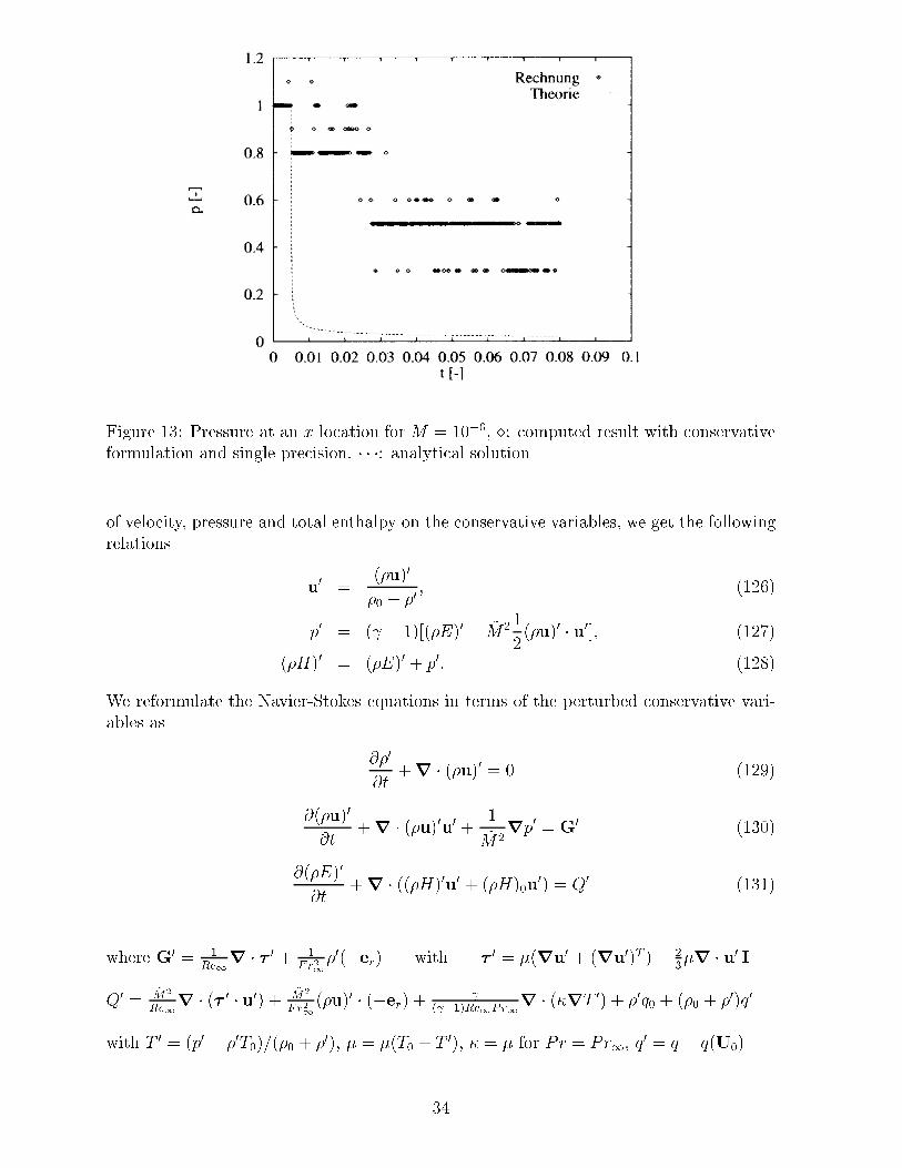
Figure 13: Pressure at an x location for M = 10�6, �: computed result with conservativeformulation and single precision, � � �: analytical solution.of velocity, pressure and total enthalpy on the conservative variables, we get the followingrelations u0 = (�u)0�0 + �0 ; (126)p0 = ( � 1)[(�E)0 � ~M2 12(�u)0 � u0]; (127)(�H)0 = (�E)0 + p0: (128)We reformulate the Navier-Stokes equations in terms of the perturbed conservative vari-ables as @�0@t +r � (�u)0 = 0 (129)@(�u)0@t +r � (�u)0u0 + 1~M2rp0 = G0 (130)@(�E)0@t +r � ((�H)0u0 + (�H)0u0) = Q0 (131)where G0 = 1Re1r � � 0 + 1Fr21�0(�er) with � 0 = �(ru0 + (ru0)T )� 23�r � u0 I.Q0 = ~M2Re1r � (� 0 � u0) + ~M2Fr21 (�u)0 � (�er) + ( �1)Re1Pr1r � (�rT 0) + �0q0 + (�0 + �0)q0with T 0 = (p0 � �0T0)=(�0 + �0), � = �(T0 + T 0), � = � for Pr = Pr1, q0 = q � q(U0).34

Figure 14: Pressure at a time instant forM = 10�6, �: computed result with conservativeformulation and single precision, � � �: analytical solution.The present perturbation formulation does not neglect anything, neither a linear nora nonlinear term: the Navier-Stokes equations in perturbation form (129), (130), (131)are analytically equal to the Navier-Stokes equations in conservative form (16), (17), (18).However, the discretization of @�0@t , rp0 and @(�E)0@t is well-conditioned opposed to @�@t , rpand @(�E)@t .In the energy equation (131), we should discretize r � (�H)0u0 as (�H)0r � u0, ofcourse, to avoid cancellation there. The shear stress tensors � 0 and � are equal, becauseu0 and u are equal. Discretizing rT 0 in (131) instead of rT in (18) avoids cancellationin the heat conduction.Central discretizations of the Navier-Stokes equations in perturbation form are asstraightforward as for the conservative form. For non-central discretizations of scalarderivatives, there is no essential di�erence either, e.g. the same one-sided �nite di�erencestencil for discretizing @p@x at a boundary can be used for @p0@x . Of course, also the initialand boundary conditions have to be formulated in perturbation form.However, if a discretization employs information based on a system of equations, e.g.a Riemann solver for the Euler equations, we must be a little bit more careful with theperturbation formulation. For example, if we need the speed of sound, we cannot simplyuse q p0=�0 but have to calculate c = q (p0 + p0)=(�0 + �0) correctly, of course. In thenext section, we shall see an example how to use an approximate Riemann solver for theEuler equations with the perturbation formulation.2.5 Characteristic Based Approximate Riemann SolverFirst, we illustrate a characteristic based approximate Riemann solver for the 2D Eulerequations in conservative form [121], [98]. Then, we show its application in perturbationform [98], [116]. 35

Figure 15: Pressure at a time instant forM = 10�2, �: computed result with conservativeformulation and single precision, dashed line: analytical solution.Let us consider the evaluation of the uxF(U) = 0BBB@ �u�u2 + 1~M2 p�uv�Hu 1CCCA ; (132)where U = (�; �u; �v; �E)T , at a cell interface xi�1=2 = 0 using the cell-centered �nitevolume approach. Neglecting multidimensional e�ects, we de�ne the Riemann problem@U@t + @F(U)@x = 0 ; �1 < x <1 ; t > 0; (133)U(x; t = 0) = ( UA for x < 0UB for x > 0 (134)As the left and right states, we choose for a �rst-order method UA = Uni�1 and UB = Uni ,i.e. the cell averages in the left cell i � 1 and the right cell i at the already calculatedtime level n. For higher order, we may use the MUSCL or ENO approach.The Jacobian matrix A = @F@U of the ux F can be diagonalizedA = R�R�1; (135)where the diagonal matrix � = diag(u� c= ~M;u; u; u+ c= ~M) contains the eigenvalues ofA. Note that c = r p�=p�1��=��1 . The 4 � 4 matrices R and R�1 contain the right and lefteigenvectors of A, respectively [50]. Using the chain rule, we write equation (133) in anon-conservative form @U@t + A@U@x = 0: (136)36

Figure 16: Entropy along the axis of the tube at a time instant forM = 10�2, �: computedresult with conservative formulation and single precision, dashed line: reference solutionwith double precision.Multiplying (136) with R�1 from the left hand side and using (135), we obtain the char-acteristic relations @W@t + �@W@x = 0; (137)where @W = R�1@U = 0BBBB@ @p� ~M�c@u@p� c2@�@v@p + ~M�c@u 1CCCCA.Thus, on the characteristics (Fig. 18), we obtain the system of ODEsdp� ~M�c du = 0 on dxdt = u� c= ~M; (138)dp� c2 d� = 0 on dxdt = u; (139)dv = 0 on dxdt = u; (140)dp+ ~M�c du = 0 on dxdt = u+ c= ~M: (141)The dimensional form of characteristic equations (138) - (141) readsdp� � ��c� du� = 0 on dx�dt� = u� � c�; (142)dp� � (c�)2 d�� = 0 on dx�dt� = u�; (143)37

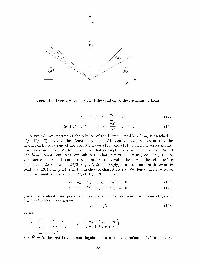
Figure 17: Typical wave pattern of the solution to the Riemann problem.dv� = 0 on dx�dt� = u�; (144)dp� + ��c� du� = 0 on dx�dt� = u� + c�: (145)A typical wave pattern of the solution of the Riemann problem (134) is sketched inFig. (Fig. 17). To solve the Riemann problem (134) approximately, we assume that thecharacteristic equations of the acoustic waves (138) and (141) even hold across shocks.Since we consider low Mach number ow, that assumption is reasonable. Because dp = 0and du = 0 across contact discontinuities, the characteristic equations (138) and (141) arevalid across contact discontinuities. In order to determine the ow at the cell interfaceat the time �t (or rather �t=2 to get O(�t2) cheaply), we �rst linearize the acousticrelations (138) and (141) as in the method of characteristics. We denote the ow state,which we want to determine by C, cf. Fig. 19, and obtainpC � pB � ~M�BcB(uC � uB) = 0; (146)pC � pA + ~M�AcA(uC � uA) = 0: (147)Since the x-velocity and pressure in regions A and B are known, equations (146) and(147) de�ne the linear system A� = �; (148)whereA = 1 � ~M�BcB1 ~M�AcA ! ; � = pB � ~M�BcBuBpA + ~M�AcAuA !for � = (pC ; uC)T .For ~M 6= 0, the matrix A is non-singular, because the determinant of A is non-zero.38

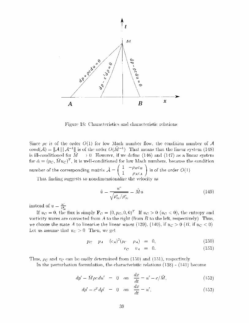
Figure 18: Characteristics and characteristic relations.Since �c is of the order O(1) for low Mach number ow, the condition number of Acond(A) = kAk kA�1k is of the order O( ~M�1). That means that the linear system (148)is ill-conditioned for ~M �! 0. However, if we de�ne (146) and (147) as a linear systemfor ~� = (pC ; ~MuC)T , it is well-conditioned for low Mach numbers, because the conditionnumber of the corresponding matrix ~A = 1 ��BcB1 �AcA ! is of the order O(1).That �nding suggests to nondimensionalize the velocity asu = u�qp�1=��1 = ~Mu (149)instead of u = u�u�1 .If uC = 0, the ux is simply FC = (0; pC; 0; 0)T . If uC > 0 (uC < 0), the entropy andvorticity waves are convected from A to the right (from B to the left, respectively). Thus,we choose the state A to linearize the linear waves (139), (140), if uC > 0 (B, if uC < 0).Let us assume that uC > 0. Then, we getpC � pA � (cA)2(�C � �A) = 0; (150)vC � vA = 0: (151)Thus, �C and vC can be easily determined from (150) and (151), respectively.In the perturbation formulation, the characteristic relations (138) - (141) becomedp0 � ~M�c du0 = 0 on dxdt = u0 � c= ~M; (152)dp0 � c2 d�0 = 0 on dxdt = u0; (153)39

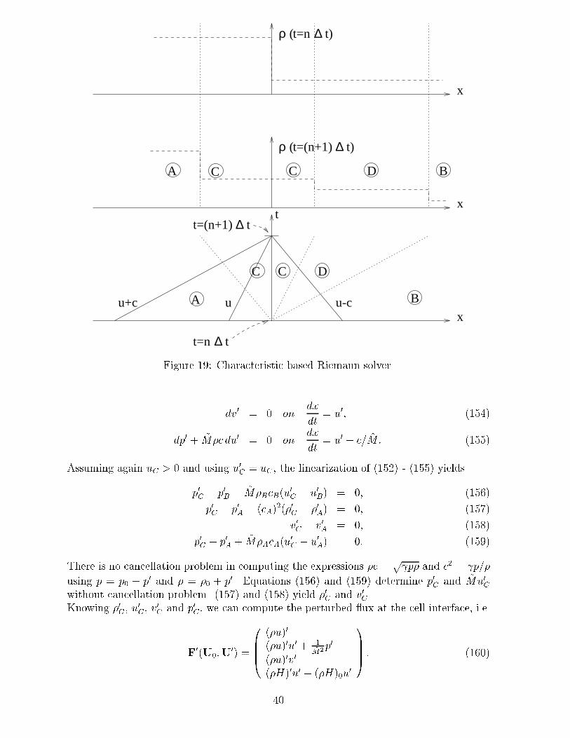
t=(n+1) ∆ tρ ( )

∆ tt=nρ ( )

t=(n+1) ∆ t

∆ tt=n

BDCCA

B

DCC

Ax

x

x

t

u+c u u-c

Figure 19: Characteristic based Riemann solver.dv0 = 0 on dxdt = u0; (154)dp0 + ~M�c du0 = 0 on dxdt = u0 + c= ~M: (155)Assuming again uC > 0 and using u0C = uC , the linearization of (152) - (155) yieldsp0C � p0B � ~M�BcB(u0C � u0B) = 0; (156)p0C � p0A � (cA)2(�0C � �0A) = 0; (157)v0C � v0A = 0; (158)p0C � p0A + ~M�AcA(u0C � u0A) = 0: (159)There is no cancellation problem in computing the expressions �c = p p� and c2 = p=�using p = p0 + p0 and � = �0 + p0. Equations (156) and (159) determine p0C and ~Mu0Cwithout cancellation problem. (157) and (158) yield �0C and v0C .Knowing �0C , u0C , v0C and p0C , we can compute the perturbed ux at the cell interface, i.e.F0(U0;U0) = 0BBB@ (�u)0(�u)0u0 + 1~M2p0(�u)0v0(�H)0u0 + (�H)0u0 1CCCA : (160)40

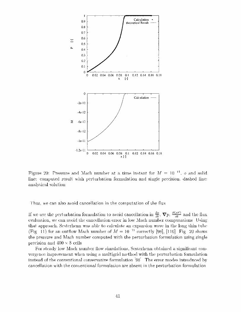
Figure 20: Pressure and Mach number at a time instant for M = 10�11, � and solidline: computed result with perturbation formulation and single precision, dashed line:analytical solution.Thus, we can also avoid cancellation in the computation of the ux.If we use the perturbation formulation to avoid cancellation in @�@t , rp, @(�E)@t and the uxevaluation, we can avoid the cancellation error in low Mach number computations. Usingthat approach, Sesterhenn was able to calculate an expansion wave in the long thin tube(Fig. 11) for an out ow Mach number of M = 10�11 correctly [98], [116]. Fig. 20 showsthe pressure and Mach number computed with the perturbation formulation using singleprecision and 400� 8 cells.For steady low Mach number ow simulations, Sesterhenn obtained a signi�cant con-vergence improvement when using a multigrid method with the perturbation formulationinstead of the conventional conservative formulation [98]. The error modes introduced bycancellation with the conventional formulation are absent in the perturbation formulation.41

3 Conclusions3.1 Asymptotic AnalysisA single time and space scale asymptotic analysis of the compressible Navier-Stokes equa-tions is shown to lead to the low Mach number equations in the zero Mach number limit.The low Mach number equations allow for large density and temperature variations, forexample in combustion. The pressure is split into the sum of the large global thermody-namic pressure and the very small 'incompressible' pressure. The global thermodynamicpressure is constant in space and may only vary in time due to nonzero volume ow andnonzero net heat conduction and heat release rate in the domain of interest. The 'in-compressible' pressure only appears in the momentum equation and is determined in asimilar way as in incompressible ow. However, the velocity divergence is in general notzero but depends on heat conduction and heat release rate as well as the time changeof the global thermodynamic pressure. Since density and temperature are related by theequation of state to the global thermodynamic pressure, any variation of the very small'incompressible' pressure does not a�ect density and temperature. Therefore, acoustics isremoved from the low Mach number equations.A multiple time scale, single space scale asymptotic analysis of the compressibleNavier-Stokes equations at low Mach numbers splits the pressure into the sum of thelarge global thermodynamic pressure, the small acoustic pressure and the very small 'in-compressible' pressure. The analysis reveals in which way the heat release rate and heatconduction a�ect the global thermodynamic pressure, the divergence of velocity and thematerial change of density at low Mach numbers. The asymptotic analysis identi�es theacoustic time change of the heat release rate as the dominant source of sound in lowMach number ow. The sound generation and propagation are governed by an inhomo-geneous wave equation for the acoustic pressure. If the ow equations are averaged overan acoustic wave period, the averaged velocity tensor describes the net acoustic e�ect onthe averaged ow �eld. Removing acoustics from the equations altogether leads again tothe low Mach number equations.3.2 Numerical ImplicationsThe low Mach number asymptotics provides a guidance for the choice of the equations.If we are not interested in acoustic e�ects in low speed combustion for example, wecan use the low Mach number equations to avoid the numerical trouble caused by thefast acoustic waves. If the compressible Euler or Navier-Stokes equations are solved atlow Mach number, the large disparity of ow velocity and speed of sound introduces asti�ness, which is absent in incompressible ow. The sti�ness can be removed by propertime derivative preconditioning for steady ow. For unsteady ow, semi-implicit methodscan treat the sti� and non-sti� terms appropriately. The large length scale disparity in lowMach number aeroacoustics calls for �ne grids and highly accurate numerical methods.Non-re ecting boundary conditions at arti�cial boundaries are decisive for the accuracyand convergence of unsteady and steady low Mach number ow simulations, respectively.Since the discretization of the small changes of the thermodynamic variables like thepressure in low Mach number ow is ill-conditioned, it leads to cancellation errors. Thecancellation problem can be avoided by discretizing the perturbation form of the Navier-Stokes equations. The changes of the conservative variables with respect to stagnationconditions are considered as the unknowns. Since the stagnation state is assumed to be42

constant in space and time, the resulting perturbation equations are not much di�erentfrom the conventional conservative form. As the discretization of the perturbation formis well-conditioned, cancellation errors are avoided. A characteristic based approximateRiemann solver is introduced. It yields a simple ux evaluation with the �nite volumemethod and is well suited for low Mach number ows with discontinuities. The implemen-tation of the perturbation form is detailed for the ux evaluation with the characteristicbased approximate Riemann solver. Using the perturbation form, even very low Machnumber ow problems can be accurately solved with single precision.AcknowledgementsThe author acknowledges the contributions to part 2 by Dr. J. Sesterhenn and Prof.H. Thomann, Institute of Fluid Dynamics, ETH Z�urich. Most of the author's researchpresented in these lecture notes was performed at the Institute of Fluid Dynamics, ETHZ�urich. Part of the research for part 1 was done during a stay with Prof. P.J. Zandber-gen's group at the Faculty of Applied Mathematics, University of Twente. Since 1998, thepresent research has been supported by TFR, the Swedish Research Council for Engineer-ing Sciences, under the author's project title \Numerical Simulation of Vortex Sound".The inspiring atmosphere at the Department of Scienti�c Computing, Uppsala University,is gratefully acknowledged.References[1] J. Lighthill. A General Introduction to Aeroacoustics and Atmospheric Sound, pages3{40. Computational Aeroacoustics. Springer-Verlag, New York, 1993. Edited byJ.C. Hardin and M.Y. Hussaini.[2] D.G. Crighton. Computational Aeroacoustics for Low Mach Number Flows, pages50{68. Computational Aeroacoustics. Springer-Verlag, New York, 1993. Edited byJ.C. Hardin and M.Y. Hussaini.[3] G. Volpe. Performance of compressible ow codes at low Mach numbers. AIAAJournal, 31:49{56, 1993.[4] S. Klainerman and A. Majda. Compressible and incompressible uids. Communi-cations on Pure and Applied Mathematics, 35:629{651, 1982.[5] H.-O. Kreiss, J. Lorenz, and M.J. Naughton. Convergence of the solutions of thecompressible to the solutions of the incompressible Navier-Stokes equations. Ad-vances in Applied Mathematics, 12:187{214, 1991.[6] A. Majda. Compressible Fluid Flow and Systems of Conservation Laws in SeveralSpace Variables. Springer-Verlag, New York, 1984.[7] J.K. Hunter, A. Majda, and R. Rosales. Resonantly interacting, weakly nonlin-ear hyperbolic waves. II. Several space variables. Studies in Applied Mathematics,75:187{226, 1986. 43

[8] A. Majda, R. Rosales, and M. Schonbek. A canonical system of integrodi�erentialequations arising in resonant nonlinear acoustics. Studies in Applied Mathematics,79:205{262, 1988.[9] R.F. Almgren. High-frequency acoustic waves in a reacting gas. SIAM Journal ofApplied Mathematics, 51:351{373, 1991.[10] R.G. Rehm and H.R. Baum. The equations of motion for thermally driven buoyant ows. Journal of Research of the National Bureau of Standards, 83:297{308, 1978.[11] Fedorchenko A.T. A model of unsteady subsonic ow with acoustics excluded.Journal of Fluid Mechanics, 334:135{155, 1997.[12] G.P. Zank and W.H. Matthaeus. The equations of nearly incompressible uids. I.Hydrodynamics, turbulence, and waves. The Physics of Fluids A, 3:69{82, 1991.[13] R. Klein. Semi-implicit extension of a Godunov-type scheme based on low Machnumber asymptotics I: One-dimensional ow. Journal of Computational Physics,121:213{237, 1995.[14] B. M�uller. Computation of compressible low Mach number ow. Habilitation thesis,ETH Z�urich, 1996.[15] B. M�uller. Low Mach number asyptotics of the Navier-Stokes equations. Journalof Engineering Mathematics, 34:97{109, 1998.[16] J.R. Ristorcelli. A closure for the compressibility of the source terms in Lighthill'sacoustic analogy. ICASE Report No. 97-44, 1997.[17] A. Majda and J. Sethian. The derivation and numerical solution of the equations forzero Mach number combustion. Combustion Science and Technology, 42:185{205,1985.[18] H.-O. Kreiss and J. Lorenz. Initial-Boundary Value Problems and the Navier-StokesEquations. Academic Press, New York, 1989.[19] W. Schneider. Mathematische Methoden der Str�omungsmechanik. Vieweg, Braun-schweig, 1978.[20] A.H. Nayfeh. Introduction to Perturbation Techniques. John Wiley & Sons, NewYork, 1981.[21] H.A. Dwyer. Calculation of low Mach number reacting ows. AIAA Journal, 28:98{105, 1990.[22] J.J. Keller. Thermoacoustic oscillations in combustion chambers of gas turbines.AIAA Journal, 33:2280{2287, 1995.[23] G.H. Schneider. Kompression und Expansion eines Gases in einem Zylinder alsSt�orungsproblem. PhD thesis, TU Wien, 1977.[24] R. Klein and N. Peters. Cumulative e�ects of weak pressure waves during the induc-tion period of a thermal explosion in a closed cylinder. Journal of Fluid Mechanics,187:197{230, 1988. 44

[25] R.H. Rhadwan and D.R. Kassoy. The response of a con�ned gas to a thermaldisturbance: Rapid boundary heating. Journal of Engineering Mathematics, 18:133{156, 1984.[26] J. Kevorkian and J.D. Cole. Multiple Scale and Singular Perturbation Methods.Springer-Verlag, New York, 1996.[27] A.P. Dowling. Thermoacoustic Sources and Instabilities, pages 378{405. ModernMethods in Analytical Acoustics. Springer-Verlag, London, 1992. Lecture Notes byD.G. Crighton and A.P. Dowling and J.E. Ffowcs Williams and M. Heckl and F.G.Leppington.[28] P. Clavin. Premixed combustion and gasdynamics. Annual Review of Fluid Me-chanics, 26:321{352, 1994.[29] J. Lighthill. On sound generated aerodynamically. I. General theory. Proceedingsof the Royal Society of London A, 211:564{587, 1952.[30] H.-O. Kreiss. Problems with Di�erent Time Scales and Acoustics, pages 156{166.Computational Aeroacoustics. Springer-Verlag, New York, 1993. Edited by J.C.Hardin and M.Y. Hussaini.[31] A.P. Dowling and J.E. Ffowcs Williams. Sound and Sources of Sound. Ellis HorwoodLimited, Chichester, 1983.[32] M. Roger. Fundamentals of aero-acoustics. Applied Aero-Acoustics: PredictionMethods, VKI Lecture Series 1996-04, 1996.[33] V.L. Wells and R.A. Renaut. Computing aerodynamically generated noise. AnnualReview of Fluid Mechanics, 29:161{199, 1997.[34] A.S. Lyrintzis. Review: The use of Kirchho�'s method in computational aeroacous-tics. Journal of Fluids Engineering, 116:665{676, 1994.[35] C.K.W. Tam. Computational aeroacoustics: Issues and methods. AIAA Journal,33:1788{1796, 1995.[36] M. Hardin. Computational approaches to aeroacoustics. Applied Aero-Acoustics:Prediction Methods, VKI Lecture Series 1996-04, 1996.[37] H. Reister. Numerische Simulation der Wechselwirkung von Druckwellen mit lam-inaren und turbulenten Grenzschichten. PhD thesis, Universit�at Karlsruhe andDFVLR-FB 87-18, 1987.[38] C.J. Moore. The role of shear-layer instability waves in jet exhaust noise. Journalof Fluid Mechanics, 80:321{367, 1977.[39] B. Gustafsson, H.-O. Kreiss, and J. Oliger. Time Dependent Problems and Di�er-ence Methods. John Wiley & Sons, New York, 1995.[40] S. K. Lele. Compact �nite di�erence schemes with spectral-like resolution. Journalof Computational Physics, 103:16{42, 1992.45

[41] W. M�ohring. On vortex sound at low Mach number. Journal of Fluid Mechanics,85:685{691, 1978.[42] W. M�ohring. Modelling Low Mach Number Noise, pages 85{96. Mechanics of SoundGeneration in Flows. Springer-Verlag, Berlin, 1979. Edited by E.-A. M�uller.[43] B. Engquist and A. Majda. Absorbing boundary conditions for the numerical sim-ulation of waves. Mathematics of Computation, 31:629{651, 1977.[44] M.B Giles. Nonre ecting boundary conditions for Euler equation calculations. AIAAJournal, 28:2050{2058, 1990.[45] D. Kr�oner. Absorbing boundary conditions for the linearized Euler equations in2-D. Mathematics of Computation, 57:153{167, 1991.[46] A.P. Saxer and M.B Giles. Quasi-three-dimensional nonre ecting boundary condi-tions for Euler equations calculations. Journal of Propulsion and Power, 9:263{271,1993.[47] L. Ferm and B. Gustafsson. A down-stream boundary procedure for the Eulerequations. Computers Fluids, 10:261{276, 1982.[48] L. Ferm. Non-re ecting boundary conditions for the steady Euler equations. Journalof Computational Physics, 122:307{316, 1995.[49] A. Verho�. Modeling of computational and solid surface boundary conditions for uid dynamics calculations. AIAA Paper 85-1496-CP, 1985.[50] C. Hirsch. Numerical Computation of Internal and External Flows. John Wiley &Sons, Chichester, 1990. Volume 2.[51] K.W. Thompson. Time dependent boundary conditions for hyperbolic systems.Journal of Computational Physics, 68:1{24, 1987.[52] K.W. Thompson. Time-dependent boundary conditions for hyperbolic systems, II.Journal of Computational Physics, 89:439{461, 1990.[53] A. Bayliss and E. Turkel. Far �eld boundary conditions for compressible ows.Journal of Computational Physics, 48:182{199, 1982.[54] C.K.W. Tam and J.C. Webb. Dispersion-relation-preserving �nite di�erenceschemes for computational acoustics. Journal of Computational Physics, 107:262{281, 1993.[55] B. M�uller. In uence of Inlet and Outlet Boundary Conditions in Internal FlowComputations at Low Mach Numbers, pages 637{643. 3rd ECCOMAS CFD Con-ference, Paris, 9-13 Sept. 1996. John Wiley & Sons, Chichester, 1996. Edited byJ.-A. D�esid�eri, C. Hirsch, P. LeTallec, M. Pandol�, and J. P�eriaux.[56] B. Gustafsson and A. Sundstr�om. Incompletely parabolic problems in uid dynam-ics. SIAM Journal on Applied Mathematics, 35:343{357, 1978.46

[57] L. Halpern. Arti�cial boundary conditions for incompletely parabolic perturbationsof hyperbolic systems. SIAM Journal on Mathematical Analysis, 22:1256{1283,1991.[58] G. Lill. Exact and approximate boundary conditions at arti�cial boundaries.Preprint Nr. 1478, FB Mathematik, TH Darmstadt, 1992.[59] J. Nordstr�om. The use of characteristic boundary conditions for the Navier-Stokesequations. Computers Fluids, 24:609{623, 1995.[60] T.J. Poinsot and S.K. Lele. Boundary conditions for direct simulations of compress-ible viscous ows. Journal of Computational Physics, 101:104{129, 1992.[61] T. Colonius, S.K. Lele, and P. Moin. Boundary conditions for direct computationof aerodynamic sound generation. AIAA Journal, 31:1574{1582, 1993.[62] M. Baum, T.J. Poinsot, and D. Th�evenin. Accurate boundary conditions for mul-ticomponent reactive ows. Journal of Computational Physics, 116:247{261, 1994.[63] H. Atkins and J. Casper. Nonre ective boundary conditions for high-order methods.AIAA Journal, 32:512{518, 1994.[64] J. Lighthill. Waves in Fluids. Cambridge University Press, Cambridge, 1978.[65] L.D. Landau and E.M. Lifshitz. Fluid Mechanics. Pergamon Press, Oxford, 2ndedition, 1993.[66] A.D. Pierce. Acoustics: An Introduction to Its Physical Priciples and Applications.Acoustical Society of America, Woodbury, 2nd edition, 1991.[67] R.R. Mankbadi. Transition, Turbulence, and Noise: Theory and Applications forScientists and Engineers. Kluwer Academic Publishers, Boston, 1994.[68] J.C. Hardin and M.Y. Hussaini, editors. Computational Aeroacoustics, New York,1993. Springer-Verlag.[69] S.K. Lele, P. Moin, T. Colonius, and B. Mitchell. Direct Computations of Aeroa-coustic Noise, pages 325{334. Computational Aeroacoustics. Springer-Verlag, NewYork, 1993. Edited by J.C. Hardin and M.Y. Hussaini.[70] Z. Haras and S. Ta'asan. Finite di�erence schemes for long-time integration. Journalof Computational Physics, 114:265{279, 1994.[71] F.Q. Hu, M.Y. Hussaini, and J.L. Manthey. Low-dissipation and low-dispersionRunge-Kutta schemes for computational acoustics. Journal of ComputationalPhysics, 124:177{191, 1996.[72] J.P. Thomas and P.L. Roe. Development of non-dissipative numerical schemes forcomputational aeroacoustics. AIAA Paper 93-3382-CP, 1993.[73] R. Vichnevetsky and J.B. Bowles. Fourier Analysis of Numerical Approximationsof Hyperbolic Equations. SIAM, Philadelphia, 1982.47

[74] M. Streng, H. Kuerten, J. Broeze, and B. Geurts. Parallel algorithms for DNS ofcompressible ow. In "Progress and Challenges in CFD Methods and Algorithms",AGARD-CP-578, pp. 23-1 to 23-10, 1996.[75] R.I. Issa. Solution of the implicitly discretized uid ow equations by operator-splitting. Journal of Computational Physics, 62:40{65, 1986.[76] J.P. Van Doormaal, G.D. Raithby, and B.H. McDonald. The segregated approach topredicting viscous compressible uid ows. Transactions of the ASME, 109:268{277,1987.[77] C.M. Rhie. Pressure-based Navier-Stokes solver using the multigrid method. AIAAJournal, 27:1017{1018, 1989.[78] K.C. Karki and S.V. Patankar. Pressure based calculation procedure for viscous ows at all speeds in arbitrary con�gurations. AIAA Journal, 27:1167{1174, 1989.[79] J.J. McGuirk and G.J. Page. Shock capturing using a pressure-correction method.AIAA Journal, 28:1751{1757, 1990.[80] S.M.H. Kariman and G.E. Schneider. Pressure-based control-volume �nite elementmethod for ow at all speeds. AIAA Journal, 33:1611{1618, 1995.[81] M.H. Kobayashi and J.C.F. Pereira. Characteristic-based pressure correction at allspeeds. AIAA Journal, 34:272{280, 1996.[82] H. Bijl and P. Wesseling. A Numerical Method for the Computation of Compress-ible Flow with Low Mach Number Regions, pages 206{212. 3rd ECCOMAS CFDConference, Paris, 9-13 Sept. 1996. John Wiley & Sons, Chichester, 1996. Editedby J.-A. D�esid�eri, C. Hirsch, P. LeTallec, M. Pandol�, and J. P�eriaux.[83] C.L. Merkle, S. Venkateswaran, and P.E.O. Buelow. The relationship betweenpressure-based and density-based algorithms. AIAA Paper 92-0425, 1992.[84] B. van Leer, W.-T. Lee, and P. Roe. Characteristic time-stepping or local precon-ditioning of the Euler equations. AIAA Paper 91-1552-CP, 1991.[85] D. Choi and C.L. Merkle. Application of time-iterative schemes to incompressible ow. AIAA Journal, 23:1518{1524, 1985.[86] M.K. Strelets and M.L. Shur. Methods of scaling the compressibility in calculatingstationary ows of a viscous gas at arbitrary Mach numbers. U.S.S.R. Computa-tional Mathematics and Mathematical Physics, 28:165{173, 1988.[87] A.G. Godfrey, R.W. Walters, and B. van Leer. Preconditioning for the Navier-Stokesequations with �nite-rate chemistry. AIAA Paper 93-0535, 1993.[88] R. Radespiel, E. Turkel, and N. Kroll. Assessment of preconditioning methods.DLR Forschungsbericht 95-29, 1995.[89] B. Koren and B. van Leer. Analysis of preconditioning and multigrid for Euler ows with low-subsonic regions. Advances in Computational Mathematics, 4:127{144, 1995. 48

[90] B. Koren. Condition improvement for point relaxation in multigrid, subsonic Euler- ow computations. Applied Numerical Mathematics, 16:457{469, 1995.[91] R.H. Pletcher and K.-H. Chen. On solving the compressible Navier-Stokes equationsfor unsteady ows at very low Mach numbers. AIAA Paper 93-3368, 1993.[92] L.-E. Eriksson. A Preconditioned Navier-Stokes Solver for Low Mach Number Flow,pages 199{205. 3rd ECCOMAS CFD Conference, Paris, 9-13 September 1996. JohnWiley & Sons, Chichester, 1996. Edited by J.-A. D�esid�eri, C. Hirsch, P. LeTallec,M. Pandol�, and J. P�eriaux.[93] D. Choi and C.L. Merkle. The application of preconditioning in viscous ows.Journal of Computational Physics, 105:207{223, 1993.[94] C.L. Merkle, S. Venkateswaran, and M. Deshpande. Convergence acceleration ofthe Navier-Stokes equations through time-derivative preconditioning. In "Progressand Challenges in CFD Methods and Algorithms", AGARD-CP-578, 1996.[95] E. Turkel. Review of preconditioning methods for uid dynamics. Applied NumericalMathematics, 12:257{284, 1993.[96] B. M�uller, J. Sesterhenn, and H. Thomann. Preconditioning and Flux Vector Split-ting for Compressible Low Mach Number Flow, pages 125{129. 13th InternationalConference on Numerical Methods in Fluid Dynamics. Springer-Verlag, Berlin, 1993.Edited by M. Napolitano and F. Sabetta.[97] J. Sesterhenn, B. M�uller, and H. Thomann. Flux-vector splitting for compressiblelow Mach number ow. Computers Fluids, 22:441{451, 1993.[98] J. Sesterhenn. Zur numerischen Berechnung kompressibler Str�omungen bei kleinenMach-Zahlen. PhD thesis, ETH Z�urich Nr. 11334, 1995.[99] K.-H. Chen and R.H. Pletcher. Primitive variable, strongly implicit calculationprocedure for viscous ows at all speeds. AIAA Journal, 29:1241{1249, 1991.[100] J. Guerra and B. Gustafsson. A numerical method for incompressible and com-pressible ow problems with smooth solutions. Journal of Computational Physics,63:377{397, 1986.[101] B. Gustafsson. Unsymmetric hyperbolic systems and the Euler equations at lowMach numbers. Journal of Scienti�c Computing, 2:123{136, 1987.[102] B. Gustafsson and H. Stoor. Navier-Stokes equations for almost incompressible ow.SIAM Journal on Numerical Analysis, 28:1523{1547, 1991.[103] V. Casulli and D. Greenspan. Pressure method for the numerical solution of tran-sient, compressible uid ows. International Journal for Numerical Methods inFluids, 4:1001{1012, 1984.[104] G. Patnaik, R.H. Guirguis, J.P. Boris, and E.S. Oran. A barely implicit correctionfor ux-corrected transport. Journal of Computational Physics, 71:1{20, 1987.49

[105] K.J. Geratz, R. Klein, C.D. Munz, and S. Roller. Multiple Pressure Variable (MPV)Approach for Low Mach Number Flows Based on Asymptotic Analysis, pages 340{354. Flow Simulation with High-Performance Computers II. Vieweg, Braunschweig,1996. Edited by E.H. Hirschel.[106] O.C. Zienkiewicz, J. Szmelter, and J. Peraire. Compressible and incompressible ow, An algorithm for all seasons. Computer Methods in Applied Mechanics andEngineering, 78:105{121, 1990.[107] O.C. Zienkiewicz and J. Wu. A general explicit or semi-explicit algorithm for com-pressible and incompressible ows. International Journal for Numerical Methods inEngineering, 35:457{479, 1992.[108] J.P. Collins, P. Colella, and H.M. Glaz. An Unsplit Implicit-Explicit GodunovMethod for Compressible Gas Dynamics, pages 659{666. 1st ECCOMAS CFD Con-ference, Brussels, 7-11 Sept. 1992. Elsevier, Amsterdam, 1992. Edited by C. Hirsch,J. P�eriaux, and W. Kordulla.[109] G. Erlebacher, M.Y. Hussaini, H.-O. Kreiss, and S. Sarkar. The analysis and simu-lation of compressible turbulence. Theoretical and Computational Fluid Dynamics,2:73{95, 1990.[110] S. Abarbanel, P. Duth, and D. Gottlieb. Splitting methods for low Mach numberEuler and Navier-Stokes equations. Computers Fluids, 17:1{12, 1989.[111] S.G. Rubin and P.K. Khosla. A review of reduced Navier-Stokes computations forcompressible viscous ows. Computing Systems in Engineering, 1:549{562, 1990.[112] M.-S. Liou and C. Ste�en. A new ux splitting scheme. Journal of ComputationalPhysics, 107:23{39, 1993.[113] A. Jameson. Arti�cial di�usion, upwind biasing, limiters and their e�ect on accuracyand multigrid convergence in transonic and hypersonic ows. AIAA Paper 93-3359,1993.[114] C. L. Merkle and Y.-H. Choi. Computation of low-speed ow with heat addition.AIAA Journal, 25:831{838, 1987.[115] A. Dadone and M. Napolitano. A perturbative lambda formulation. AIAA Journal,24:411{417, 1986.[116] J. Sesterhenn, B. M�uller, and H. Thomann. On the Cancellation Problem in Cal-culating Compressible Low Mach Number Flows, pages 408{413. 3rd ECCOMASCFD Conference, Paris, 9-13 September 1996. John Wiley & Sons, Chichester, 1996.Edited by J.-A. D�esid�eri, C. Hirsch, P. LeTallec, M. Pandol�, and J. P�eriaux.[117] W.R. Briley, H. McDonald, and S.J. Shamroth. A low Mach number Euler formu-lation and application to time-iterative LBI schemes. AIAA Journal, 21:1467{1469,1983.[118] M. Hafez, M. Soliman, and S. White. A uni�ed approach for numerical simulation ofviscous compressible and incompressible ows over adiabatic and isothermal walls."5th Symposium on Numerical and Physical Aspects of Aerodynamic Flows", LongBeach, CA, 1992. 50

[119] M.T. Heath. Scienti�c Computing: An Introductory Survey. McGraw-Hill, NewYork, 1997.[120] F. Aebli and H. Thomann. Stability of the ow behind a pressure pulse in a tube.Zeitschrift f�ur angewandte Mathematik und Physik, 39:387{396, 1988.[121] J. Sesterhenn, B. M�uller, and H. Thomann. A Simple Characteristic Flux Evaluationfor Subsonic Flow, pages 57{61. 2nd ECCOMAS CFD Conference, Stuttgart, 5-8 Sept. 1994. John Wiley & Sons, Chichester, 1994. Edited by S. Wagner, E.H.Hirschel, J. P�eriaux, and R. Piva.

51