Exponential decay to equilibrium for a fibre lay-down process on a

moving conveyor belt

Emeric Bouin∗ Franca Hoffmann† Clement Mouhot ‡

September 26, 2018

Abstract

We show existence and uniqueness of a stationary state for a kinetic Fokker-Planck equationmodelling the fibre lay-down process in the production of non-woven textiles. Following amicro-macro decomposition, we use hypocoercivity techniques to show exponential convergenceto equilibrium with an explicit rate assuming the conveyor belt moves slow enough. This workis an extension of (Dolbeault et al., 2013), where the authors consider the case of a stationaryconveyor belt. Adding the movement of the belt, the global Gibbs state is not known explicitly.We thus derive a more general hypocoercivity estimate from which existence, uniqueness andexponential convergence can be derived. To treat the same class of potentials as in (Dolbeaultet al., 2013), we make use of an additional weight function following the Lyapunov functionalapproach in (Kolb et al., 2013).

Key-words: Hypocoercivity, rate of convergence, fibre lay-down, existence and uniqueness of astationary state, perturbation, moving belt,AMS Class. No: 35B20, 35B40, 35B45, 35Q84

1 Introduction

The mathematical analysis of the fibre lay-down process in the production of non-woven textiles hasseen a lot of interest in recent years [14, 15, 6, 10, 11, 4, 12]. Non-woven materials are produced inmelt-spinning operations: hundreds of individual endless fibres are obtained by continuous extrusionthrough nozzles of a melted polymer. The nozzles are densely and equidistantly placed in a row ata spinning beam. The visco-elastic, slender and in-extensible fibres lay down on a moving conveyorbelt to form a web, where they solidify due to cooling air streams. Before touching the conveyorbelt, the fibres become entangled and form loops due to highly turbulent air flow. In [14] a generalmathematical model for the fibre dynamics is presented which enables the full simulation of theprocess. Due to the huge amount of physical details, these simulations of the fibre spinning andlay-down usually require an extremely large computational effort and high memory storage, see

∗CEREMADE - Universite Paris-Dauphine, UMR CNRS 7534, Place du Marechal de Lattre de Tassigny, 75775Paris Cedex 16, France (bouin@ceremade.dauphine.fr).

†CCA, Centre for Mathematical Sciences, University of Cambridge, Wilberforce Road, Cambridge CB3 0WA, UK(fkoh2@cam.ac.uk).

‡DPMMS, Centre for Mathematical Sciences, University of Cambridge, Wilberforce Road, Cambridge CB3 0WA,UK (c.mouhot@dpmms.cam.ac.uk).

1

arX

iv:1

605.

0412

1v3

[m

ath.

AP]

14

Apr

201

7

[15]. Thus, a simplified two-dimensional stochastic model for the fibre lay-down process, togetherwith its kinetic limit, is introduced in [6]. Generalisations of the two-dimensional stochastic model[6] to three dimensions have been developed by Klar et al. in [10] and to any dimension d ≥ 2 byGrothaus et al. in [7].

We now describe the model we are interested in, which comes from [6]. We track the positionx(t) ∈ R2 and the angle α(t) ∈ S1 of the fibre at the lay-down point where it touches the conveyorbelt. Interactions of neighbouring fibres are neglected. If x0(t) is the lay-down point in the coordi-nate system following the conveyor belt, then the tangent vector of the fibre is denoted by τ(α(t))with τ(α) = (cosα, sinα). Since the extrusion of fibres happens at a constant speed, and the fibresare in-extensible, the lay-down process can be assumed to happen at constant normalised speed‖x′0(t)‖ = 1. If the conveyor belt moves with constant speed κ in direction e1 = (1, 0), then

dx

dt= τ(α) + κe1.

Note that the speed of the conveyor belt cannot exceed the lay-down speed: 0 ≤ κ ≤ 1. The fibredynamics in the deposition region close to the conveyor belt are dominated by the turbulent air flow.Applying this concept, the dynamics of the angle α(t) can be described by a deterministic forcemoving the lay-down point towards the equilibrium x = 0 and by a Brownian motion modellingthe effect of the turbulent air flow. We obtain the following stochastic differential equation for therandom variable Xt = (xt, αt) on R2 × S1,dxt = (τ(αt) + κe1) dt,

dαt =[−τ⊥(αt) · ∇xV (xt)

]dt+AdWt ,

(1)

where Wt denotes a one-dimensional Wiener process, A > 0 measures its strength relative to thedeterministic forcing, τ⊥ = (− sinα, cosα), and V : R2 −→ R is an external potential carryinginformation on the coiling properties of the fibre. More precisely, since a curved fibre tends back toits starting point, the change of the angle α is assumed to be proportional to τ⊥(α) ·∇xV (x). It hasbeen shown in [12] that under suitable assumptions on the external potential V , the fibre lay downprocess (1) has a unique invariant distribution and is even geometrically ergodic (see Remark 1.2).The stochastic approach yields exponential convergence in total variation norm, however withoutexplicit rate. We will show here that a stronger result can be obtained with a functional analysisapproach. Our argument uses crucially the construction of an additional weight functional for thefibre lay-down process in the case of unbounded potential gradients inspired by [12, Proposition3.7].

The probability density function f(t, x, α) corresponding to the stochastic process (1) is governedby the Fokker-Planck equation

∂tf + (τ + κe1) · ∇xf − ∂α(τ⊥ · ∇xV f

)= D∂ααf (2)

with diffusivity D = A2/2. We state below assumptions on the external potential V that will beused regularly throughout the paper:

(H1) Regularity and symmetry : V ∈ C2(R2) and V is spherically symmetric outside someball B(0, RV ).

2

(H2) Normalisation:∫R2 e

−V (x) dx = 1.

(H3) Spectral gap condition (Poincare inequality): there exists a positive constant Λ suchthat for any u ∈ H1(e−V dx) with

∫R2 ue

−V dx = 0,∫R2

|∇xu|2 e−V dx ≥ Λ

∫R2

u2e−V dx.

(H4) Pointwise regularity condition on the potential : there exists c1 > 0 such that for anyx ∈ R2, the Hessian ∇2

xV of V (x) satisfies

|∇2xV (x)| ≤ c1(1 + |∇xV (x)|).

(H5) Behaviour at infinity :

lim|x|→∞

|∇xV (x)|V (x)

= 0, lim|x|→∞

|∇2xV (x)|

|∇xV (x)|= 0 .

Remark 1.1. Assumptions (H2-3-4) are as stated in [4]. Assumption (H1) assumes regularity ofthe potential that is stronger and included in that discussed in [4] since (H1) implies V ∈W 2,∞

loc (R2).Assumption (H5) is only necessary if the potential gradient |∇xV | is unbounded. Both boundedand unbounded potential gradients may appear depending on the physical context, and we will treatthese two cases separately where necessary. A typical example for an external potential satisfyingassumptions (H1-2-3-4-5) is given by

V (x) = K(1 + |x|2

)s/2(3)

for some constants K > 0 and s ≥ 1 [5, 12]. The potential (3) satisfies (H3) since

lim inf|x|→∞

(|∇xV |2 − 2∆xV

)> 0 ,

see for instance [17, A.19. Some criteria for Poincare inequalities, page 135]. The other assump-tions are trivially satisfied as can be checked by direct inspection. In this family of potentials, thegradient ∇xV is bounded for s = 1 and unbounded for s > 1.

Remark 1.2. The proof of ergodicity in [12] assumes that the potential satisfies

lim|x|→∞

|∇xV (x)|V (x)

= 0 , lim|x|→∞

|∇2xV (x)|

|∇xV (x)|= 0 , lim

|x|→∞|∇xV (x)| =∞ . (4)

Under these assumptions, there exists an invariant distribution ν to the fibre lay-down process (1),and some constants C(x0) > 0, λ > 0 such that

‖Px0,α0 (Xt ∈ ·)− ν‖TV ≤ C(x0)e−λt ,

where ‖·‖TV denotes the total variation norm. The stochastic Lyapunov technique applied in [12]however does not give any information on how the constant C(x0) depends on the initial positionx0, or how the rate of convergence λ depends on the conveyor belt speed κ, the potential V and the

3

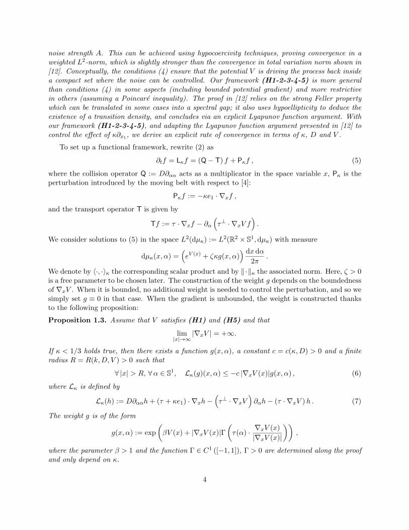
noise strength A. This can be achieved using hypocoercivity techniques, proving convergence in aweighted L2-norm, which is slightly stronger than the convergence in total variation norm shown in[12]. Conceptually, the conditions (4) ensure that the potential V is driving the process back insidea compact set where the noise can be controlled. Our framework (H1-2-3-4-5) is more generalthan conditions (4) in some aspects (including bounded potential gradient) and more restrictivein others (assuming a Poincare inequality). The proof in [12] relies on the strong Feller propertywhich can be translated in some cases into a spectral gap; it also uses hypoellipticity to deduce theexistence of a transition density, and concludes via an explicit Lyapunov function argument. Withour framework (H1-2-3-4-5), and adapting the Lyapunov function argument presented in [12] tocontrol the effect of κ∂x1, we derive an explicit rate of convergence in terms of κ, D and V .

To set up a functional framework, rewrite (2) as

∂tf = Lκf = (Q− T) f + Pκf , (5)

where the collision operator Q := D∂αα acts as a multiplicator in the space variable x, Pκ is theperturbation introduced by the moving belt with respect to [4]:

Pκf := −κe1 · ∇xf ,

and the transport operator T is given by

Tf := τ · ∇xf − ∂α(τ⊥ · ∇xV f

).

We consider solutions to (5) in the space L2(dµκ) := L2(R2 × S1,dµκ) with measure

dµκ(x, α) =(eV (x) + ζκg(x, α)

) dx dα

2π.

We denote by 〈·, ·〉κ the corresponding scalar product and by ‖·‖κ the associated norm. Here, ζ > 0is a free parameter to be chosen later. The construction of the weight g depends on the boundednessof ∇xV . When it is bounded, no additional weight is needed to control the perturbation, and so wesimply set g ≡ 0 in that case. When the gradient is unbounded, the weight is constructed thanksto the following proposition:

Proposition 1.3. Assume that V satisfies (H1) and (H5) and that

lim|x|→∞

|∇xV | = +∞.

If κ < 1/3 holds true, then there exists a function g(x, α), a constant c = c(κ,D) > 0 and a finiteradius R = R(k,D, V ) > 0 such that

∀ |x| > R, ∀α ∈ S1, Lκ(g)(x, α) ≤ −c |∇xV (x)|g(x, α) , (6)

where Lκ is defined by

Lκ(h) := D∂ααh+ (τ + κe1) · ∇xh−(τ⊥ · ∇xV

)∂αh− (τ · ∇xV )h . (7)

The weight g is of the form

g(x, α) := exp

(βV (x) + |∇xV (x)|Γ

(τ(α) · ∇xV (x)

|∇xV (x)|

)),

where the parameter β > 1 and the function Γ ∈ C1 ([−1, 1]), Γ > 0 are determined along the proofand only depend on κ.

4

We show in Section 3 the existence of such a weight function g under appropriate conditionsfollowing ideas from [12].

We denote C := C∞c(R2 × S1

), and define the orthogonal projection Π on the set of local

equilibria Ker Q

Πf :=

∫S1f

dα

2π,

and the mass Mf of a given distribution f ∈ L2(dµκ),

Mf :=

∫R2×S1

fdxdα

2π.

Integrating (2) over R2 × S1 shows that the mass of solutions of (2) is conserved over time, andstandard maximum principle arguments show that it remains non-negative for non-negative initialdata. The collision operator Q is symmetric and satisfies

∀ f ∈ C, 〈Qf, f〉0 = −D ‖∂αf‖20 ≤ 0 ,

i.e. Q is dissipative in L2(dµ0). Further, we have TΠf = e−V τ · ∇xuf for f ∈ C, with uf := eV Πf ,which implies ΠTΠ = 0 on C. Since the transport operator T is skew-symmetric with respect to〈· , ·〉0,

〈Lκf, f〉0 = 〈Qf, f〉0 + 〈Pκf, f〉0for any f in C. In the case κ = 0, if the entropy dissipation −〈Qf, f〉0 was coercive with respectto the norm ‖ · ‖0, exponential decay to zero would follow as t → ∞. However, such a coercivityproperty cannot hold since Q vanishes on the set of local equilibria. Instead, Dolbeault et al. [5]applied a strategy called hypocoercivity (as theorised in [17]) and developed by several groups in the2000s, see for instance [9, 8, 13, 2, 3]. The full hypocoercivity analysis of the long time behaviourof solutions to this kinetic model in the case of a stationary conveyor belt, κ = 0, is completed in[4]. For technical applications in the production process of non-wovens, one is interested in a modelincluding the movement of the conveyor belt, and our aim is to extend the results in [4] to smallκ > 0.

We follow the approach of hypocoercivity for linear kinetic equations conserving mass developedin [5], with several new difficulties. Considering the case κ = 0, Q and T are closed operators onL2(dµ0) such that Q − T generates the C0-semigroup e(Q−T)t on L2(dµ0). When κ > 0, we usethe additional weight function g > 0 to control the perturbative term Pκ in the case of unboundedpotential gradients; and show the existence of a C0-semigroup for Lκ = Q − T + Pκ (see Section4.1). Unless otherwise specified, all computations are performed on the operator core C, and canbe extended to L2(dµκ) by density arguments.

When κ = 0, the hypocoercivity result in [5, 4] is based on: microscopic coercivity, whichassumes that the restriction of Q to (Ker Q)⊥ is coercive, and macroscopic coercivity, which is aspectral gap-like inequality for the operator obtained when taking a parabolic drift-diffusion limit,in other words, the restriction of T to Ker Q is coercive. The two properties are satisfied in the caseof a stationary conveyor belt:

• The operator Q is symmetric and the Poincare inequality on S1,

1

2π

∫S1|∂αf |2 dα ≥ 1

2π

∫S1

(f − 1

2π

∫S1f dα

)2

dα,

5

implies that −〈Qf, f〉0 ≥ D ‖(1− Π)f‖20.

• The operator T is skew-symmetric and for any h ∈ L2(dµ0) such that uh = eV Πh ∈H1(e−V dx) and

∫R2×S1 hdµ0 = 0, (H3) implies

‖TΠh‖20 =1

4π

∫R2×S1

e−V |∇xuh|2 dx dα ≥ Λ

4π

∫R2×S1

e−V u2h dx dα =

Λ

2‖Πh‖20 .

In the case κ = 0, the unique global normalised equilibrium distribution F0 = e−V lies in theintersection of the null spaces of T and Q. When κ > 0, F0 is not in the kernel of Pκ and we are notable to find the global Gibbs state of (5) explicitly. However, the hypocoercivity theory is basedon a priori estimates [5] that are, as we shall prove, to some extent stable under perturbation. Ourmain result reads:

Theorem 1.4. Let fin ∈ L2(dµκ) and let (H1-2-3-4-5) hold. For 0 < κ < 1 small enough (with aquantitative estimate) and ζ > 0 large enough (with a quantitative estimate), there exists a uniquenon-negative stationary state Fκ ∈ L2(dµκ) with unit mass MFκ = 1. In addition, for any solutionf of (2) in L2(dµκ) with mass Mf and subject to the initial condition f(t = 0) = fin, we have

‖f(t, ·)−MfFκ‖κ ≤ C ‖fin −MfFκ‖κ e−λκt , (8)

where the rate of convergence λκ > 0 depends only on κ, D and V , and the constant C > 0 dependsonly on D and V .

In the case of a stationary conveyor belt κ = 0 considered in [4], the stationary state is charac-terised by the eigenpair (Λ0, F0) with Λ0 = 0, F0 = e−V , and so Ker L0 = 〈F0〉. This means thatthere is an isolated eigenvalue Λ0 = 0 and a spectral gap of size at least [−λ0, 0] with the rest ofthe spectrum Σ(L0) to the left of −λ0 in the complex plane. Adding the movement of the conveyorbelt, Theorem 1.4 shows that Ker Lκ = 〈Fκ〉 and the exponential decay to equilibrium with rateλκ corresponds to a spectral gap of size at least [−λκ, 0]. Further, it allows to recover an explicitexpression for the rate of convergence λ0 for κ = 0 (see Step 5 in Section 2.1). In general, we are notable to compute the stationary state Fκ for κ > 0 explicitly, but Fκ converges to F0 = e−V weaklyas κ→ 0 (see the discussion in Section 5). Let us finally emphasize that a specific contribution ofour paper is to introduce two (and not one as in [5, 4]) modifications of the entropy: 1) we firstmodify the space itself with the coercivity weight g, then 2) we change the norm with an auxiliaryoperator following the hypocoercivity approach.

The rest of the paper deals with the case κ > 0 and is organised as follows. In Section 2, weprove the main hypocoercivity estimate. This allows us to establish the existence of solutions to (2)using semigroup theory and to deduce the existence and uniqueness of a steady state in Section 4by a contraction argument. In Section 3, we give a detailed definition of the weight function g thatis needed for the hypocoercivity estimate in Section 2.

2 Hypocoercivity estimate

Following [5] we introduce the auxiliary operator

A := (1 + (TΠ)∗(TΠ))−1(TΠ)∗ ,

6

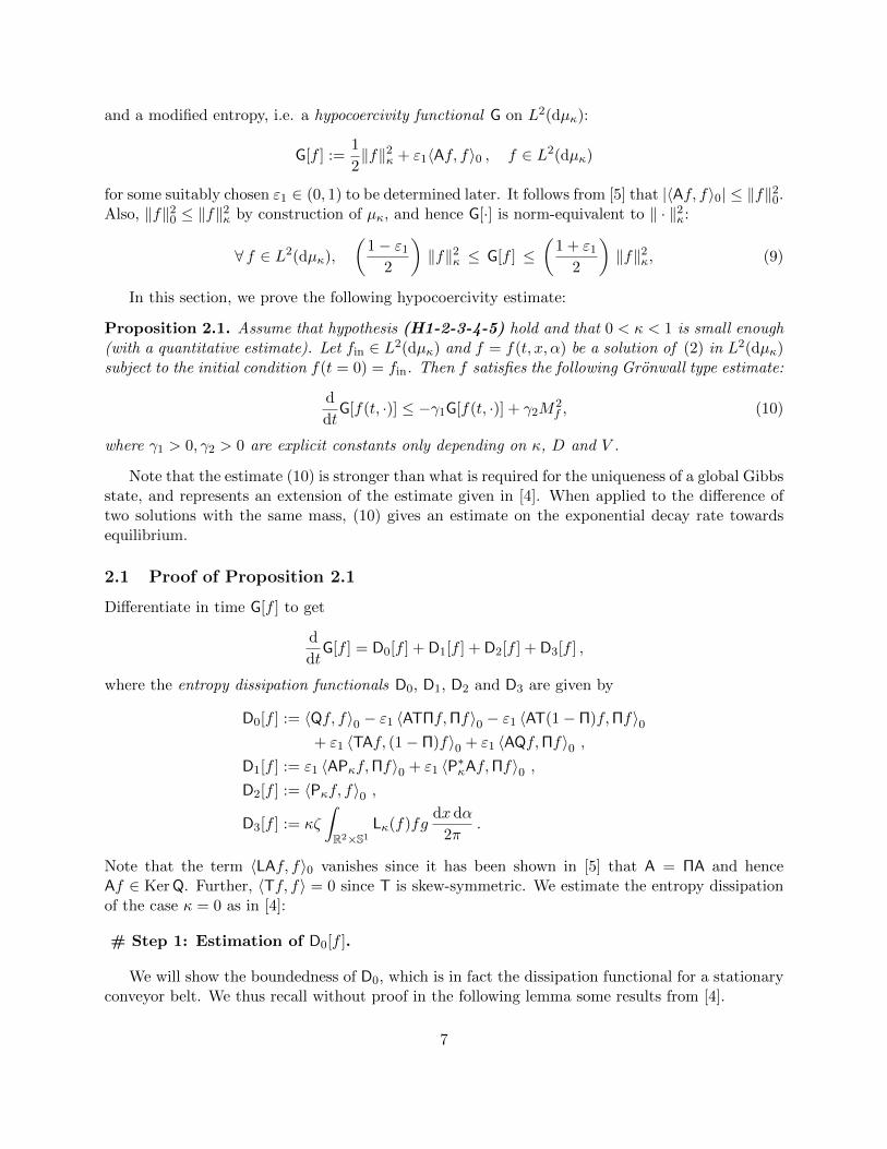
and a modified entropy, i.e. a hypocoercivity functional G on L2(dµκ):

G[f ] :=1

2‖f‖2κ + ε1〈Af, f〉0 , f ∈ L2(dµκ)

for some suitably chosen ε1 ∈ (0, 1) to be determined later. It follows from [5] that |〈Af, f〉0| ≤ ‖f‖20.Also, ‖f‖20 ≤ ‖f‖2κ by construction of µκ, and hence G[·] is norm-equivalent to ‖ · ‖2κ:

∀ f ∈ L2(dµκ),

(1− ε1

2

)‖f‖2κ ≤ G[f ] ≤

(1 + ε1

2

)‖f‖2κ, (9)

In this section, we prove the following hypocoercivity estimate:

Proposition 2.1. Assume that hypothesis (H1-2-3-4-5) hold and that 0 < κ < 1 is small enough(with a quantitative estimate). Let fin ∈ L2(dµκ) and f = f(t, x, α) be a solution of (2) in L2(dµκ)subject to the initial condition f(t = 0) = fin. Then f satisfies the following Gronwall type estimate:

d

dtG[f(t, ·)] ≤ −γ1G[f(t, ·)] + γ2M

2f , (10)

where γ1 > 0, γ2 > 0 are explicit constants only depending on κ, D and V .

Note that the estimate (10) is stronger than what is required for the uniqueness of a global Gibbsstate, and represents an extension of the estimate given in [4]. When applied to the difference oftwo solutions with the same mass, (10) gives an estimate on the exponential decay rate towardsequilibrium.

2.1 Proof of Proposition 2.1

Differentiate in time G[f ] to get

d

dtG[f ] = D0[f ] + D1[f ] + D2[f ] + D3[f ] ,

where the entropy dissipation functionals D0, D1, D2 and D3 are given by

D0[f ] := 〈Qf, f〉0 − ε1 〈ATΠf,Πf〉0 − ε1 〈AT(1− Π)f,Πf〉0+ ε1 〈TAf, (1− Π)f〉0 + ε1 〈AQf,Πf〉0 ,

D1[f ] := ε1 〈APκf,Πf〉0 + ε1 〈P∗κAf,Πf〉0 ,D2[f ] := 〈Pκf, f〉0 ,

D3[f ] := κζ

∫R2×S1

Lκ(f)fgdx dα

2π.

Note that the term 〈LAf, f〉0 vanishes since it has been shown in [5] that A = ΠA and henceAf ∈ Ker Q. Further, 〈Tf, f〉 = 0 since T is skew-symmetric. We estimate the entropy dissipationof the case κ = 0 as in [4]:

# Step 1: Estimation of D0[f ].

We will show the boundedness of D0, which is in fact the dissipation functional for a stationaryconveyor belt. We thus recall without proof in the following lemma some results from [4].

7

Lemma 2.2 (Dolbeault et al. [4]). The following estimates hold:

〈Qf, f〉0 ≤ −‖(1− Π)f‖20 , ‖AT(1− Π)f‖0 ≤ CV ‖(1− Π)f‖0 ,

‖AQf‖0 ≤D

2‖(1− Π)f‖0 , ‖TAf‖0 ≤ ‖(1− Π)f‖0 .

In order to control the contribution 〈ATΠf,Πf〉0 in D0, we note that

ATΠ = (1 + (TΠ)∗TΠ)−1 (TΠ)∗TΠ

shares its spectral decomposition with (TΠ)∗TΠ, and by macroscopic coercivity

〈(TΠ)∗TΠf, f〉0 = ‖TΠf‖20 =∥∥TΠ(f −Mfe

−V )∥∥2

0≥ Λ

2

∥∥Π(f −Mfe−V )

∥∥2

0.

Hence,

〈ATΠf, f〉0 ≥Λ/2

1 + Λ/2

∥∥Π(f −Mfe−V )

∥∥2

0.

Now, recalling Lemma 2.2 and using∥∥Π(f −Mfe

−V )∥∥2

0= ‖Πf‖20 −M2

f , we estimate

D0[f ] ≤(ε1 −D) ‖(1− Π)f‖20 + ε1λ2 ‖(1− Π)f‖0 ‖Πf‖0 − ε1γ2

(‖Πf‖20 −M

2f

),

with λ2 := CV +D/2 > 0 and γ2 := Λ/21+Λ/2 > 0.

# Step 2: Estimation of D1[f ].

We now turn to the entropy dissipation functional D1, which we will estimate using ellipticregularity. Instead of bounding APκ, we apply an elliptic regularity strategy to its adjoint, as forAT(1− Π) in [4]. Let f ∈ L2(dµ0) and define h := (1 + (TΠ)∗TΠ)−1 f so that uh = eV Πh satisfies

Πf = e−V uh + ΠT∗T(e−V uh

)= e−V uh −

1

2∇x ·

(e−V∇xuh

).

We have used here the fact that in the space L2(dµ0):{T = τ · ∇x − ∂α

[(τ⊥ · ∇xV

)],

T∗ = −τ · ∇x +(τ⊥ · ∇xV

)∂α − (τ · ∇xV ) .

ThenA∗f = TΠh = e−V τ · ∇xuh ,

and since the adjoint for 〈·, ·〉0 of the perturbation operator Pκ is given by

P∗κ = −Pκ − PκV ,

8

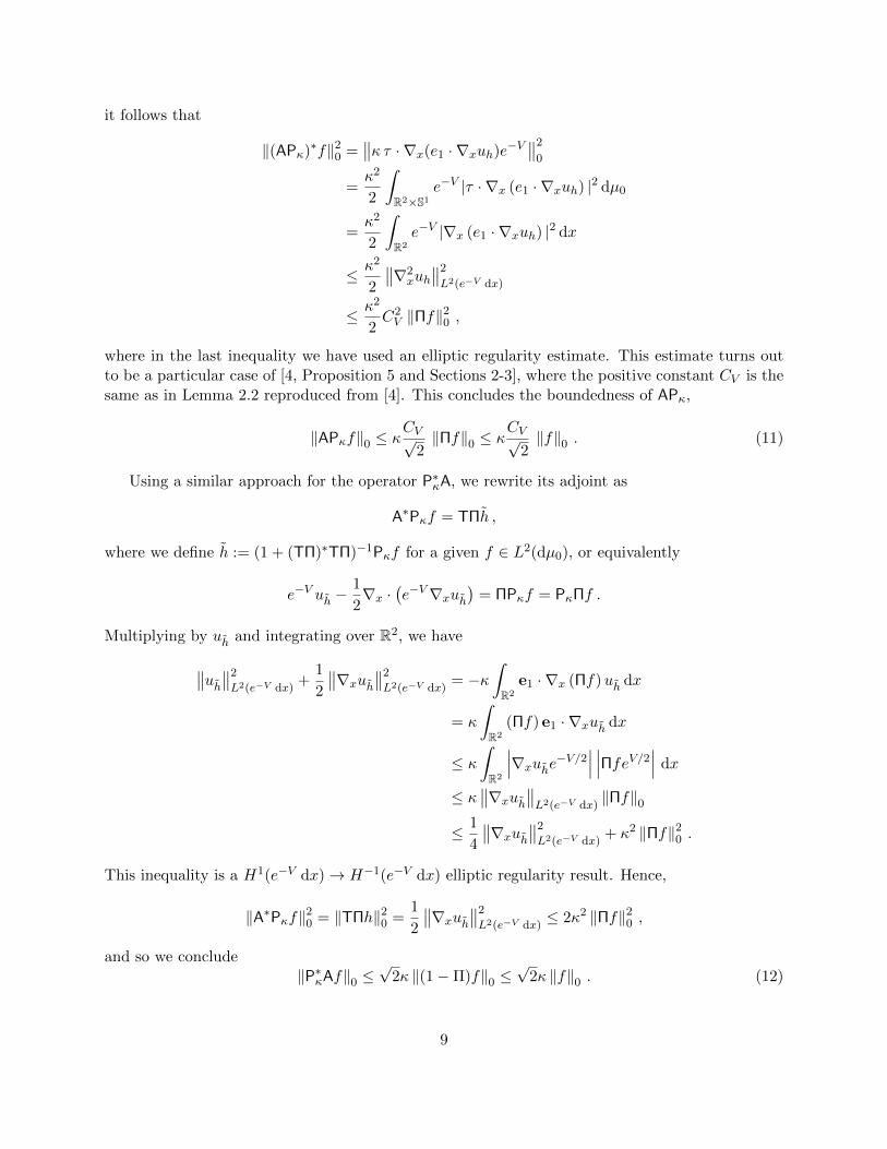
it follows that

‖(APκ)∗f‖20 =∥∥κ τ · ∇x(e1 · ∇xuh)e−V

∥∥2

0

=κ2

2

∫R2×S1

e−V |τ · ∇x (e1 · ∇xuh) |2 dµ0

=κ2

2

∫R2

e−V |∇x (e1 · ∇xuh) |2 dx

≤ κ2

2

∥∥∇2xuh∥∥2

L2(e−V dx)

≤ κ2

2C2V ‖Πf‖

20 ,

where in the last inequality we have used an elliptic regularity estimate. This estimate turns outto be a particular case of [4, Proposition 5 and Sections 2-3], where the positive constant CV is thesame as in Lemma 2.2 reproduced from [4]. This concludes the boundedness of APκ,

‖APκf‖0 ≤ κCV√

2‖Πf‖0 ≤ κ

CV√2‖f‖0 . (11)

Using a similar approach for the operator P∗κA, we rewrite its adjoint as

A∗Pκf = TΠh ,

where we define h := (1 + (TΠ)∗TΠ)−1Pκf for a given f ∈ L2(dµ0), or equivalently

e−V uh −1

2∇x ·

(e−V∇xuh

)= ΠPκf = PκΠf .

Multiplying by uh and integrating over R2, we have

∥∥uh∥∥2

L2(e−V dx)+

1

2

∥∥∇xuh∥∥2

L2(e−V dx)= −κ

∫R2

e1 · ∇x (Πf)uh dx

= κ

∫R2

(Πf) e1 · ∇xuh dx

≤ κ∫R2

∣∣∣∇xuhe−V/2∣∣∣ ∣∣∣ΠfeV/2∣∣∣ dx

≤ κ∥∥∇xuh∥∥L2(e−V dx)

‖Πf‖0

≤ 1

4

∥∥∇xuh∥∥2

L2(e−V dx)+ κ2 ‖Πf‖20 .

This inequality is a H1(e−V dx)→ H−1(e−V dx) elliptic regularity result. Hence,

‖A∗Pκf‖20 = ‖TΠh‖20 =1

2

∥∥∇xuh∥∥2

L2(e−V dx)≤ 2κ2 ‖Πf‖20 ,

and so we conclude‖P∗κAf‖0 ≤

√2κ ‖(1−Π)f‖0 ≤

√2κ ‖f‖0 . (12)

9

Combining (11) and (12), the entropy dissipation functional D1 is bounded by

D1[f ] ≤ κε1

(CV√

2+√

2

)‖f‖20 = 2κλ1 ‖f‖20,

where we defined λ1 := 12

(CV√

2+√

2)

.

# Step 3: Estimation of D2[f ].

Using integration by parts, we have

〈Pκf, f〉0 =κ

2

∫R2×S1

(e1 · ∇xV ) f2eVdx dα

2π.

The estimation of this term goes differently depending on the boundedness of ∇xV .If ∇xV is bounded, we write

D2[f ] ≤ |〈Pκf, f〉0| ≤κ

2‖∇xV ‖∞‖f‖20 =

κ

2‖∇xV ‖∞‖f‖2κ,

where we have used ‖f‖κ = ‖f‖0, since g ≡ 0.Assume now that |∇xV | → ∞ as |x| → ∞. Thanks to the choice of g, we have the estimate

D2[f ] ≤ |〈Pκf, f〉0| ≤κ

2

∫R2×S1

|∇xV |f2eVdx dα

2π≤ κ

2C3

∫R2×S1

f2gdx dα

2π, (13)

withC3 := sup

x∈R2

(|∇xV |eV g−1

),

which is finite by (H5).

# Step 4: Estimation of D3[f ].

We start by recalling that this estimate is only relevant when ∇xV is unbounded. Indeed, inthe opposite case, D3[f ] = 0 since g ≡ 0 by definition. By the identity∫

R2×S1Lκ(f)fg dx dα =

1

2

∫R2×S1

Lκ(g)f2 dx dα−D∫R2×S1

|∂αf |2 g dx dα

with Lκ as defined in (7), we have

D3[f ] ≤ κζ(

1

2

∫R2×S1

Lκ(g)f2 dx dα

2π

). (14)

Proposition 1.3 allows us to control the g-weighted L2-norm outside some fixed ball. More precisely,take R > 0 in (6) large enough s.t. |∇xV | ≥ 1 for all |x| > R, then∫

R2×S1Lκ(g)f2 dx dα

2π

≤∫S1

∫|x|<R

Lκ(g)f2 dx dα

2π− c

∫S1

∫|x|>R

|∇xV |f2gdx dα

2π

≤∫S1

∫|x|<R

((Lκ(g) + cg) e−V

)f2eV

dx dα

2π− c

∫R2×S1

f2gdx dα

2π

≤ C4(R)‖f‖20 − c∫R2×S1

f2gdx dα

2π, (15)

10

where C4(R) := sup|x|≤R(|Lκ(g) + cg|e−V

).

Remark 2.3. Observe here that one could take advantage of the growth of ∇xV by playing withthe cut-off parameter R and keeping track of min|x|≥R |∇xV | in the negative term. It could leadto more optimal constants but we chose instead to vary the parameter ζ in front of the coercivityweight g in the measure µκ for simplicity.

# Step 5: Putting the four previous steps together.

Combine the previous steps into

D0[f ] + D1[f ] ≤(ε1 −D) ‖(1− Π)f‖20 + ε1λ2 ‖(1− Π)f‖0 ‖Πf‖0

− ε1γ2

(‖Πf‖20 −M

2f

)+ 2κλ1 ‖f‖20

=− (D − ε1 − 2κλ1) ‖(1− Π)f‖20 + ε1λ2 ‖(1− Π)f‖0 ‖Πf‖0− (ε1γ2 − 2κλ1) ‖Πf‖20 + ε1γ2M

2f

≤−(D − ε1 − 2κλ1 −

ε1λ2b

2

)‖(1− Π)f‖20

−(ε1γ2 − 2κλ1 −

ε1λ2

2b

)‖Πf‖20 + ε1γ2M

2f

≤− 2ξ(κ)‖f‖20 + ε1γ2M2f ,

by Young’s inequality with the choice b = λ2/γ2, and where we used the fact that ‖(1 − Π)f‖20 +‖Πf‖20 = ‖f‖20. Here, ξ(κ) is explicit, and given by

ξ(κ) :=1

2min

{D − ε1

(1 +

λ22

2γ2

),ε1γ2

2

}− κλ1

=Dγ2

2

2(γ2

2 + 2γ2 + λ22

) − κλ1 ,

since the minimum in the first term is realised when the two arguments are equal, fixing ε1 =2Dγ2/

(γ2

2 + 2γ2 + λ22

). Note that this choice of ε1 satisfies ε1 < D and ε1 < 1. Choosing κ small

enough ensures ξ(κ) > 0. From this analysis we conclude

D0[f ] + D1[f ] ≤ −2ξ(κ)‖f‖20 + ε1γ2M2f . (16)

Let us now add the control of D2 + D3. If ∇xV is bounded, g ≡ 0 and D3 = 0:

d

dtG[f ] = D0[f ] + D1[f ] + D2[f ]

≤ − (4ξ(κ)− κ‖∇xV ‖∞)1

2‖f‖2κ + ε1γ2M

2f

≤ −γ1G[f ] + ε1γ2M2f

by the norm equivalence (9). Here, we defined

γ1 :=4ξ(κ)− κ‖∇xV ‖∞

1 + ε1> 0 .

11

When ∇xV is unbounded, (13)-(14)-(15)-(16) imply

d

dtG[f ] =D0[f ] + D1[f ] + D2[f ] + D3[f ]

≤− 2ξ(κ)‖f‖20 + ε1γ2M2f +

κ

2C3

∫R2×S1

f2gdx dα

2π

+κζ

2

(C4(R)‖f‖20 − c

∫R2×S1

f2gdx dα

2π

)=− 1

2(4ξ(κ)− κζC4(R)) ‖f‖20 −

κζ

2

(c− C3

ζ

)∫R2×S1

f2gdx dα

2π+ ε1γ2M

2f

≤− 1

2min

{4ξ(κ)− κζC4(R), c− C3

ζ

}‖f‖2κ + ε1γ2M

2f

≤− γ1 G[f ] + ε1γ2M2f

again by norm equivalence (9), and where we defined

γ1 :=1

1 + ε1min

{4ξ(κ)− κζC4(R), c− C3

ζ

}> 0 .

This requires ζ > 0 to be large enough, and the upper bound for κ should be chosen accordingly:

ζ >C3

c, 4ξ(κ)− κζC4(R) > 0 .

In order to maximise the rate of convergence to equilibrium given κ, D and V , one can optimiseγ1 over ζ whilst respecting the above constraints.

Remark 2.4. The condition γ1 > 0 translates into an explicit upper bound on κ. More precisely,we require ξ(κ) > κu/4 where u := ‖∇xV ‖∞ in the case of a bounded potential gradient, andu := ζC4(R) otherwise. This condition is satisfied for small enough κ:

0 ≤ κ < ε1γ2

(4λ1 + u)=

2Dγ22

(4λ1 + u)(γ22 + 2γ2 + λ2

2)

which also implies ξ(κ) > 0. Recall that Proposition 1.3 requires κ < 1/3 in the case of unboundedpotential gradients. These conditions provide a range of κ for which Proposition 2.1 holds.

3 The coercivity weight g

In this section, we define the function g in such a way that it allows us to control the loss of weightin the perturbation operator Pκ. When ∇xV is bounded, we do not need any extra weight sincethen we may control the perturbation thanks to the stationary weight eV , and so we set g ≡ 0 inthat case. When it is not, Proposition 1.3 provides a suitable weight function g by constructivemethods.

12

3.1 Proof of Proposition 1.3

The proof is strongly inspired from [12], however our weight is different since we work in an L2-framework rather than in an L1 one. Assuming ∇xV is unbounded, we seek a weight g of theform

g(x, α) = exp

(βV (x) + |∇xV (x)|Γ

(τ(α) · ∇xV (x)

|∇xV (x)|

)),

where the parameter β > 1 and the function Γ ∈ C1 ([−1, 1]), Γ > 0 are to be determined. Wedefine

Y (x, α) := τ(α) · ∇xV (x)

|∇xV (x)|, Y ⊥(x, α) := τ⊥(α) · ∇xV (x)

|∇xV (x)|,

and split the proof into four steps: 1) we rewrite statement (6) using the explicit expression of theweight g, 2) we simplify the obtained expression using assumption (H5), 3) we prove the equivalentstatement obtained in Step 2 by defining a suitable choice of Γ(·) and β, and 4) we demonstratethat it is indeed possible to choose suitable parameters for the calculations in Step 3 to hold, fixingexplicit expressions where possible.

# Step 1: Rewriting the weight estimate (6).

Applying the operator Lκ defined in (7) to g, we can compute explicitly

Lκ(g)

g=D

(|∇xV |∂ααΓ(Y ) + |∇xV |2|∂αΓ(Y )|2

)+ (τ(α) + κe1) · (β∇xV +∇x (|∇xV |Γ(Y )))

− |∇xV |2Y ⊥∂αΓ(Y )− |∇xV |Y .

Since∂αΓ = Y ⊥Γ′(Y ) and ∂ααΓ = ∂α

(Y ⊥Γ′(Y )

)= −Y Γ′(Y ) + |Y ⊥|2Γ′′(Y ) ,

we get

Lκ(g)

g=D

(|∇xV |

(−Y Γ′(Y ) + |Y ⊥|2Γ′′(Y )

)+ |∇xV |2|Y ⊥|2

(Γ′(Y )

)2)+ (τ(α) + κe1) · (β∇xV +∇x (|∇xV |Γ(Y )))

− |∇xV |2|Y ⊥|2Γ′(Y )− |∇xV |Y=(β − 1−DΓ′(Y ))|∇xV |Y + κβe1 · ∇xV + (τ(α) + κe1) · ∇x (|∇xV |Γ(Y ))

+ |Y ⊥|2(D|∇xV |Γ′′(Y ) + |∇xV |2

[D(Γ′(Y )

)2 − Γ′(Y )])

.

In order to see which Γ to choose, let us divide by |∇xV | and denote the diffusion and transportpart by

diff(x, α) := (τ(α) + κe1) · ∇x (|∇xV |Γ(Y ))

|∇xV |, tran(x) :=

e1 · ∇xV|∇xV |

.

Now, we can rewrite the statement of Proposition 1.3: we seek a positive constant c > 0 and aradius R > 0 such that for any α ∈ S1 and |x| > R,

(β − 1−DΓ′(Y ))Y + κβtran(x) + diff(x, α)

+ |Y ⊥|2(DΓ′′(Y ) + |∇xV |

[D(Γ′(Y )

)2 − Γ′(Y )])≤ −c .

13

To achieve this bound, note that |Y | ≤ 1 and |tran| ≤ 1 for all (x, α) ∈ R2 × S1.

# Step 2: Simplifying the weight estimate.

Further, the diffusion term diff(·) can be made arbitrarily small outside a sufficiently large ball.Indeed,

diff(x, α) = (τ + κe1) ·[Γ′ (Y )∇xY + Γ (Y )

∇x(|∇xV |)|∇xV |

],

and both |∇xY | and |∇x(|∇xV |)|/|∇xV | converge to zero as |x| → ∞ by assumption (H5), and Γis bounded. In other words, using the fact that the potential gradient is unbounded, it remains toshow that we can find constants γ > κβ > 0 and a radius r1 > 0 such that

∀|x| > r1, (β − 1−DΓ′)Y + |Y ⊥|2(DΓ′′ + |∇xV |

[D(Γ′)2 − Γ′

])≤ −γ . (17)

Then we can choose r2 > 0 such that

|x| > r2 =⇒ ∀α ∈ S1, diff(x, α) ≤ γ − κβ2

,

and we conclude for the statement of Proposition 1.3 with R := max{r1, r2} and c := (γ−κβ)/2 > 0.

# Step 3: Proof of the weight estimate.

Proving (17) can be done by an explicit construction. We define Γ′ ∈ C0([−1, 1]) piecewise,

Γ′(Y ) =

δ+ if Y > ε0 ,

δ+−δ−2ε0

(Y + ε0) + δ− if |Y | ≤ ε0 ,

δ− if Y < −ε0 ,

-1 +1−ε0 ε0

1Dδ+

δ−

Γ′(Y )

Y

Figure 1: Derivative of Γ

where 0 < δ− < δ+ < 1/D and ε0 ∈ (0, 1) are to be determined. With this choice of Γ′, we canensure that Γ is strictly positive in the interval [−1, 1]. Now, let us show that there exist suitablechoices of γ and β for the bound (17) to hold. More precisely, we choose a suitable β such that(β − 1)/D ∈ (δ−, δ+) and 0 < γ < γ, defining γ := ε0 (1 +Dδ+ − β) and γ := ε0 (β − 1−Dδ−).We split our analysis into cases:

• Assume Y > ε0. Then the LHS of (17) can be bounded as follows:

(β − 1−Dδ+)Y + δ+(Dδ+ − 1

)|∇xV ||Y ⊥|2 < (β − 1−Dδ+)ε0 = −γ .

• Assume Y < −ε0. Then the LHS of (17) can be bounded as follows:

(β − 1−Dδ−)Y + δ−(Dδ− − 1

)|∇xV ||Y ⊥|2 < −(β − 1−Dδ−)ε0 = −γ .

14

• Assume |Y | ≤ ε0. Since 1 = |Y |2 + |Y ⊥|2, we have |Y ⊥|2 ≥ 1− ε20. Further, setting

h = aY + b ∈ (δ−, δ+) , a :=δ+ − δ−

2ε0, b :=

δ+ + δ−

2,

we have Γ′ = h and Dh2 − h ≤ Dδ−(δ+ − 1/D). Now, using the fact that the potentialgradient is unbounded, we can find a radius r1 > 0 large enough such that for all |x| > r1,

D(δ+ − δ−)

2ε0−Dδ−

(1

D− δ+

)|∇xV | < −

2γ

(1− ε20).

Putting these estimates together, we obtain for |x| > r1:

(β − 1−Dh)Y + |Y ⊥|2(D(δ+ − δ−)

2ε0+ |∇xV |

[Dh2 − h

])≤ (β − 1−Dδ−)ε0 + |Y ⊥|2

(D(δ+ − δ−)

2ε0+ |∇xV |

[Dδ−

(δ+ − 1

D

)])≤ γ + (1− ε2

0)

(D(δ+ − δ−)

2ε0+ |∇xV |

[Dδ−

(δ+ − 1

D

)])≤ −γ .

# Step 4: Choice of parameters.

We now come back to the choice of δ−, δ+, ε0, β such that κβ < γ and 0 < γ < γ hold true.More precisely, these two constraints translate into the following bound on β:

1 +D

(δ+ + δ−

2

)< β <

(ε0

κ+ ε0

)(1 +Dδ+

). (18)

It is easy to see that this bound also implies 1 + Dδ− < β < 1 + Dδ+ as required. However, forthis to be possible we need to choose ε0 such that LHS < RHS, in other words,

κ

(2 +D (δ+ + δ−)

D (δ+ − δ−)

)< ε0 . (19)

Since ε0 has to be less than 1 and D(δ+− δ−)/(2 +D (δ+ + δ−)) < 1/3, this bound is only possibleif κ ∈ (0, 1/3); then it remains to choose 0 < δ− < δ+ < 1/D such that

κ <D (δ+ − δ−)

2 +D (δ+ + δ−)∈(

0,1

3

). (20)

To satisfy all these constraints, we make the choice of parameters (for κ < 1/3):

δ+ :=3(1 + κ)

4D, δ− :=

(1− 3κ)

4D.

Then (20) holds true, and we can fix ε0 ∈ (0, 1) to satisfy (19):

ε0 :=1

2

(1 + κ

(2 +D (δ+ + δ−)

D (δ+ − δ−)

))=

1

2

(1 + 9κ

1 + 3κ

).

Finally, we choose β satisfying (18) as follows:

β :=1

2

[1 +D

(δ+ + δ−

2

)+

(ε0

κ+ ε0

)(1 +Dδ+

)]=

3

4+

(1 + 9κ)(7 + 3κ)

8(6κ2 + 11κ+ 1)∈ (1, 2) .

15

4 Existence and uniqueness of a steady state

4.1 Existence of a C0-semigroup

The proof of the next theorem relies on the a priori estimates from Section 2.

Theorem 4.1. The linear operator Lκ : D(Lκ) → L2(dµκ) defined in (5) is the infinitesimalgenerator of a C0-semigroup (St)t≥0 on L2(dµκ).

Proof. Let us denote by L∗κ the adjoint of Lκ in L2(dµκ). Both domains D (Lκ) and D (L∗κ) containthe core C and are dense. The operator Lκ is closable in L2(dµκ). To see this, take a sequence(fn)n∈N ∈ D(Lκ) converging to zero in L2(dµκ) such that the sequence (Lκfn)n∈N converges to somelimit h ∈ L2(dµκ). Then for any test function ϕ ∈ C,⟨

ϕ , Lκfn⟩κ

=⟨L∗κϕ , fn

⟩κ→ 0 as n→∞ .

Since the left-hand side converges to⟨ϕ , h

⟩κ

for all ϕ ∈ C, we conclude h ≡ 0 a.e., and so Lκ

is closable. Similarly, L∗κ is closable. We denote by Lκ and L∗κ some closed extensions of Lκ andL∗κ, respectively. Lumer-Phillips Theorem in the form [16, Corollary 4.4] states that an operator Lgenerates a C0-semigroup if L is closed and both L and L∗ are dissipative. Since the core C is densein both D(Qκ) and D(Q∗κ), which in turn are both dense in L2(dµκ), then for any constant C > 0,Lκ − CId is dissipative if and only if L∗κ − CId is dissipative. Therefore, it remains to show thatLκ − CId is dissipative for some C > 0. Since the restriction of Lκ to C is Lκ, it is enough to provethat Lκ − CId is dissipative on C for some constant C > 0. The estimates in Section 2 show thatthere exists C > 0 s.t.

∀f ∈ C,⟨Lκf , f

⟩κ≤ C‖f‖2κ

for some explicit constant C > 0, which concludes the proof.

4.2 Proof of Theorem 1.4

Proposition 2.1 is the key ingredient to deduce existence of a unique steady state. The set

B :=

{f ∈ L2(dµκ) : G[f ] ≤ γ2

γ1, f ≥ 0, Mf = 1

}is convex and bounded in L2(dµκ) by the norm equivalence (9). By Theorem 4.1, the operator Lκgenerates a C0-semigroup (St)t≥0. Then let us show that B is invariant under the action of (St)t≥0.Integrating in time the hypocoercivity estimate (10) in Proposition 2.1 for any fin ∈ L2(dµκ) withmass 1, we obtain the bound

G[f(t)] ≤ G[fin]e−γ1t +γ2

γ1

(1− e−γ1t

),

and thus

∀ t > 0, G[f(t)] ≤ max

{G[fin],

γ2

γ1

}.

Since in addition, (St)t≥0 conserves mass and positivity, we conclude St(B) ⊂ B for all times.

16

Integrate again the hypocoercivity estimate (10) in Proposition 2.1, now for the difference oftwo solutions with same mass, to get

G[Stf − Sth] ≤ e−γ1tG[f − h]

for any t > 0 and f, h ∈ B. It follows by Banach’s fixed-point theorem that there exists a uniqueut ∈ B such that St(u

t) = ut for each t > 0. Let tn := 2−n, n ∈ N, and un := utn . ThenS2−n(un) = un, and by repeatedly applying the semigroup property,

∀ k ∈ N, ∀m ≤ n ∈ N, Sk2−m(un) = un . (21)

Let us prove that B is weakly compact in L2(dµκ). Consider a sequence (fn)n∈N ∈ B. It hasa cluster point f for the weak convergence since B is bounded in L2(dµκ), and the correspondingsubsequence is still denoted fn for simplicity. By lower semi-continuity of the equivalent norm G:

G[f ] ≤ lim infn→∞

G[fn] ≤ γ2/γ1 .

Further, since fn ≥ 0 for all n ∈ N, it follows that f ≥ 0 (the set of non-negative functions is astrongly closed convex set, hence weakly closed). It remains to show that the limit f has mass 1by preventing loss of mass at infinity. Use Cauchy-Schwarz’s inequality and the norm equivalence(9) to get for r > 0

(1 + κζ)

(∫|x|>r

Πfn dx

)2

≤

(∫|x|>r

∫S1f2n e

V dxdα

2π

)(∫|x|>r

∫S1e−V

dxdα

2π

)

+ κζ

(∫|x|>r

∫S1f2n g

dxdα

2π

)(∫|x|>r

∫S1g−1 dxdα

2π

)

≤ ‖fn‖2κ

(∫|x|>r

∫S1

(e−V + g−1

) dxdα

2π

)

≤(

2

1− ε1

)γ2

γ1

(∫|x|>r

∫S1

2e−Vdxdα

2π

).

This shows that

supn∈N

(∫|x|>r

Πfn dx

)

≤((

4

(1− ε1)(1 + κζ)

)(γ2

γ1

))1/2(∫|x|>r

∫S1e−V

dxdα

2π

)1/2

→ 0 as r →∞ ,

since∫R2×S1 e

−V dxdα2π = 1. Together with Mfn = 1 for all n ∈ N, it follows that Mf = 1. Hence

f ∈ B. The weak compactness of B implies the existence of a subsequence unj of un and a functionu ∈ B such that unj converges weakly to u in L2(dµκ). Letting nj →∞ in (21) implies that (sinceSt is a continuous operator)

∀m ∈ N, ∀ k ∈ N, Sk2−m(u) = u .

17

Finally the density of the dyadic rationals {k2−m : k ∈ N,m ∈ N} in (0,+∞) and continuity ofSt(u) in t for all u ∈ B imply that

∀ t ≥ 0, St(u) = u .

This shows the existence and uniqueness of a global stationary state Fκ := u ∈ B.

To complete the proof of Theorem 1.4, we apply the hypocoercivity estimate Proposition 2.1 tothe difference between a solution f ∈ L2(dµκ) and the unique stationary state of the same mass,MfFκ, to show exponential convergence to equilibrium in ‖ · ‖κ: first of all, we deduce from thecontraction estimate (10) that

G[f(t)−MfFκ] ≤ G[fin −MfFκ] e−γ1t ,

which allows then to estimate the difference to equilibrium in the L2(dµκ)-norm. Indeed, by normequivalence, we obtain

‖f(t)−MfFκ‖2κ ≤1 + ε1

1− ε1‖fin −MfFκ‖2κ e−γ1t .

Hence, we obtain (8) with rate of convergence λκ := γ1/2.

5 Concluding remarks

From our previous estimates, we have that G(Fk) is uniformly bounded in κ for κ sufficiently small.As a consequence, (Fκ)κ>0 is a relatively weakly compact family in L2(dµκ), and by uniqueness ofthe stationary state in the case κ = 0, we deduce that Fκ → F0 as κ→ 0. It could also be provedwith further work that the optimal (spectral gap) relaxation rate is continuous as κ→ 0.

Working in L2(dµκ) ⊂ L2(dµ0) we are treating the operator Lκ as a small perturbation of thecase κ = 0 with stationary conveyor belt. The natural space to investigate the convergence to Fκin the case κ > 0 however is L2

(F−1κ dx dα

). In this L2-space the transport operator T−Pκ is not

skew-symmetric and the collision operator Q is not self-adjoint, so the hypocoercivity method [5]cannot be applied. To get around this, one can split the operator Lκ differently into a transportand a collision part following the approach in [1]. More precisely, we can write Lκ = Q− T where Qf = ∂α

(D∂αf − ∂αFκ

Fκf),

Tf = (τ + κe1) · ∇xf − ∂α[(τ⊥ · ∇xV + ∂αFκ

Fκ

)f].

Then in L2(F−1κ dx dα

)the operator Q is symmetric and negative semi-definite, and the operator T

is skew-symmetric. Furthermore, the stationary state Fκ lies in the intersection of the kernels of thecollision and transport operators, i.e. Fκ ∈ Ker Q ∩ Ker T. The hypocoercivity approach requiresmicroscopic and macroscopic coercivity of Q and T. Which then requires as in [1] to control thebehaviour of the stationary state at infinity, i.e. for large enough |x|,

∀α ∈ S1, e−σ1V (x) ≤ Fκ(x, α) ≤ e−σ2V (x)

for some constants σ1, σ2 > 0. If true, this would be an important physical information on thestationary state, but we do not know how to prove it at now. Even with this information at hand,this approach requires that the existence of the stationary state is known a priori. The rate ofconvergence one obtains in this case may be different from the rate obtained here, and it is notclear which method yields the better rate as both are most likely not optimal.

18

Acknowledgments

EB is very grateful to the University of Cambridge for its sunny hospitality during the secondsemester of the academic year 2015-2016. EB and CM acknowledge the support of the ERC GrantMATKIT (ERC-2011-StG). FH acknowledges support from the Engineering and Physical SciencesResearch Council (UK) grant number EP/H023348/1 for the University of Cambridge Centre forDoctoral Training, the Cambridge Centre for Analysis. The authors are very grateful to the twoanonymous referees for very fruitful and detailed comments and remarks.

References

[1] V. Calvez, G. Raoul, and C. Schmeiser. Confinement by biased velocity jumps: aggregationof escherichia coli. Kinet. Relat. Models, 8(4):651–666, 2015.

[2] L. Desvillettes and C. Villani. On the trend to global equilibrium in spatially inhomogeneousentropy-dissipating systems: the linear Fokker-Planck equation. Comm. Pure Appl. Math.,54(1):1–42, 2001.

[3] L. Desvillettes and C. Villani. On the trend to global equilibrium for spatially inhomogeneouskinetic systems: the Boltzmann equation. Invent. Math., 159(2):245–316, 2005.

[4] J. Dolbeault, A. Klar, C. Mouhot, and C. Schmeiser. Exponential rate of convergence toequilibrium for a model describing fiber lay-down processes. Appl. Math. Res. Express. AMRX,(2):165–175, 2013.

[5] J. Dolbeault, C. Mouhot, and C. Schmeiser. Hypocoercivity for linear kinetic equations con-serving mass. Trans. Amer. Math. Soc., 367(6):3807–3828, 2015.

[6] T. Gotz, A. Klar, N. Marheineke, and R. Wegener. A stochastic model and associated Fokker-Planck equation for the fiber lay-down process in nonwoven production processes. SIAM J.Appl. Math., 67(6):1704–1717, 2007.

[7] M. Grothaus, A. Klar, J. Maringer, and P. Stilgenbauer. Geometry, mixing properties andhypocoercivity of a degenerate diffusion arising in technical textile industry. arXiv/1203.4502,2012.

[8] Y. Guo. The Landau equation in a periodic box. Comm. Math. Phys., 231(3):391–434, 2002.

[9] F. Herau and F. Nier. Isotropic hypoellipticity and trend to equilibrium for the Fokker-Planckequation with a high-degree potential. Arch. Ration. Mech. Anal., 171(2):151–218, 2004.

[10] A. Klar, J. Maringer, and R. Wegener. A 3D model for fiber lay-down in nonwoven productionprocesses. Math. Models Methods Appl. Sci., 22(9):1250020, 18, 2012.

[11] M. Kolb, M. Savov, and A. Wubker. Geometric ergodicity of a hypoelliptic diffusion modellingthe melt-spinning process of nonwoven materials. arXiv/1112.6159, 2011.

[12] M. Kolb, M. Savov, and A. Wubker. (Non-)ergodicity of a degenerate diffusion modeling thefiber lay down process. SIAM J. Math. Anal., 45(1):1–13, 2013.

19

[13] T.-P. Liu, T. Yang, and S.-H. Yu. Energy method for Boltzmann equation. Phys. D, 188(3-4):178–192, 2004.

[14] N. Marheineke and R. Wegener. Fiber dynamics in turbulent flows: general modeling frame-work. SIAM J. Appl. Math., 66(5):1703–1726 (electronic), 2006.

[15] N. Marheineke and R. Wegener. Fiber dynamics in turbulent flows: specific Taylor drag. SIAMJ. Appl. Math., 68(1):1–23 (electronic), 2007.

[16] A. Pazy. Semigroups of linear operators and applications to partial differential equations,volume 44 of Applied Mathematical Sciences. Springer-Verlag, New York, 1983.

[17] C. Villani. Hypocoercivity. Mem. Amer. Math. Soc., 202(950):iv+141, 2009.

20