Movement ecology of adfluvial bull trout (Salvelinus … ecology of adfluvial bull trout (Salvelinus confluentus) By Lee Frank Gordon Gutowsky A thesis submitted to the faculty of

Movement ecology of adfluvial bull trout (Salvelinus confluentus)

By

Lee Frank Gordon Gutowsky

A thesis submitted to the faculty of Graduate and Postdoctoral Affairs in partial

fulfillment of the requirements for the degree of Doctor of Philosophy in Biology

Carleton University

Ottawa, Ontario

©2014, Lee F.G. Gutowsky

ii

Dedication

To Victoria, who has accompanied and encouraged me through all of my graduate

studies. I also dedicate this thesis to my loving family and friends. Finally, in dedication

to my earliest and most influential academic mentors, Mrs. Millar and Mr. Hudson.

iii

Abstract

Organism movement can be explained by a combination of inter-related variables that are

derived from an individual’s internal state, environment, motion capacity, and navigation

capacity. Movement ecology can be used as a framework under which to test ecological

hypotheses across a variety of spatial and temporal scales. To reveal aspects of movement

ecology of free-ranging adfluvial bull trout (Salvelinus confluentus), I used acoustic

telemetry and tested hypotheses about thermal resource selection, diel vertical migration,

and size and sex-related effects on movement. I tagged 187 adult fish and monitored

these individuals for up to two years (2010-2012) in the ~ 425 km2 Kinbasket Reservoir,

BC. Correlates of movement included combinations of variables representing the internal

state (e.g., phenotypic traits including sex and body size), the external environment (e.g.,

temperature and diel period), and the navigation capacity (e.g., the way in which an

organism perceives and navigates its environment). Over the two-year period,

temperature experience was similar for all body sizes (~ 400-800 mm total length).

During summers, bull trout were predicted to experience temperatures that were within

~1°C of their lab-derived thermal optimum for metabolism and growth for juveniles. Bull

trout occupied temperatures between approximately 11-15°C and selected higher

temperatures as these temperatures became less available with the progression of summer

and autumn. Diel vertical migration (DVM) was evident, with the largest individuals

occupying the shallowest water. Significant DVM continued to occur during winter when

the thermal profile was presumably isothermal. Winter DVM, and a significant effect of

body size, indicated that multiple inter-related factors were responsible for vertical

movements. Body size and season were significant predictors of home range size, with

iv

the largest home ranges predicted during autumn and spring in fish greater than 700 mm

total length. A significant sex x body size interaction predicted horizontal movement such

that in a given month, large females moved significantly farther than large males and

small females, whereas there was no difference between large and small males. This

work provides novel insight into thermal resource selection, diel vertical migration, and

the correlates of horizontal movement. This research generates new information on the

movement ecology of adfluvial bull trout in a hydropower reservoir which is relevant to

understanding entrainment risk.

v

Acknowledgements

Special thanks to Philip Harrison and Eduardo Martins for their brilliant

contributions to our published manuscripts and for their openness and willingness to

share ideas and collaborate. Thanks greatly to my supervisor, Steve Cooke. Throughout

my time at Carleton Steve’s support, advice, and leadership was simply incredible.

Thanks to my Mike Power for sage advice. To those who helped in the field including

Sean Landsman, Jason Thiem, Jeff Nitychoruk, Mark Taylor, Juan Molina, Glenn

Crossin, David Patterson, Taylor Nettles, and Jayme Hills. To Phil and Jason who, while

in the field, nearly took a bullet for my thesis. Thanks to our boat captain and now friend,

Jamie Tippe. My field experience was incredible and much of this is owed to Jamie’s

great attitude, sense of humour, and dedication to conservation. Jake Brownscombe and

Tom Hossie who, regardless of the day of the week or time of day, were always keen to

converse about science. I cherish these conversations and look forward to many more.

Thanks to Alf Leake and Karen Bray for sharing valuable resources regarding Kinbasket

Reservoir. I would also like to thank Rick Chartraw for his hospitality at Kinbasket Lake

Resort. I would again like to thank my fiancé, Victoria, who was always eager to read

early drafts of my manuscripts and who continuously encouraged me to attend

conferences, workshops, and meetings for my own professional development.

vi

Co-authorship

Chapter 2: Thermal Resource selection in bull trout: temperature experience and

selection change with availability. Gutowsky, L. F. G, Harrison, P. M., Martins, E. G.,

Leake, A., Patterson, D. A., Zhu, D. Z., Power, M., Cooke, S. J.

While the work is my own, this research chapter is a collaborative effort among a

number of researchers. I came up with the original idea, performed all of the analyses,

and conducted all of the writing. Data were interpreted by LFGG, SJC, and MP. PMH,

EGM, DAP, and SJC were involved with field work. AL, DAP, MP, DZZ, and SJC

provided financial support. The manuscript is in the process of submission.

Chapter 3: Diel vertical migration hypotheses explain size-dependent behaviour in

bull trout. Gutowsky, L. F. G., Harrison, P. M., Martins, E. G., Leake, A., Patterson, D.

A., Power, M., Cooke S. J.

This study is my own yet there are a number of coauthors whose contributions

were invaluable to its completion. PMH, MP, and I generated the original idea to

examine diel vertical migration (DVM) in the context of DVM hypotheses. I performed

all of the analyses and conducted all of the writing. EGM provided feedback on the

statistics. PMH, EGM, DAP, and SJC were involved with the field work. AL, DAP, MP,

and SJC provided financial support. All co-authors provided feedback on the manuscript

which has been published with the following citation:

vii

Gutowsky, L. F. G., Harrison, P. M., E. G. Martins, A. Leake, Power, M., Cooke, S. J.

2013. Diel vertical migration hypotheses explain size-dependent behavior in a

freshwater piscivore. Anim. Behav. 86: 365-373.

Chapter 4: Sex and body size influence the spatial ecology of bull trout. Gutowsky,

L. F. G, Harrison, P. M., Martins, E. G., Leake, A., Patterson, D. A., Power, M., Cooke,

S. J.

Although the research is my own, this study could not have been completed

without the help of a number of coauthors. I generated the original idea for this paper,

performed all the analyses, and wrote the manuscript. PMH, EGM, DAP, and SJC were

present during the field season. AL, DAP, MP, and SJC provided financial support. All of

the authors provided valuable feedback on drafts of this manuscript which is currently in

its second round of revisions.

viii

Table of Contents

Dedication ....................................................................................................................... ii

Abstract .......................................................................................................................... iii

Acknowledgements ......................................................................................................... v

Co-authorship ................................................................................................................. vi

List of Tables .................................................................................................................. x

List of Figures ................................................................................................................ xi

Chapter 1: General Introduction ..................................................................................... 1

Bull trout ..................................................................................................................... 5

Study location ............................................................................................................. 9

Chapter 2: Thermal resource selection in bull trout: temperature experience and

selection change with availability ................................................................................. 16

Abstract ..................................................................................................................... 16

Introduction ............................................................................................................... 18

Methods..................................................................................................................... 21

Results ....................................................................................................................... 29

Discussion ................................................................................................................. 31

Tables ........................................................................................................................ 39

Figures....................................................................................................................... 42

Chapter 3: Diel vertical migration hypotheses explain size-dependent behaviour in bull

trout ............................................................................................................................... 46

Abstract ..................................................................................................................... 46

Introduction ............................................................................................................... 48

Methods..................................................................................................................... 50

Results ....................................................................................................................... 54

Discussion ................................................................................................................. 57

Tables ........................................................................................................................ 62

Figures....................................................................................................................... 65

Chapter 4: Sex and body size influences on the movement ecology of bull trout ........ 70

Abstract ..................................................................................................................... 70

Introduction ............................................................................................................... 72

ix

Methods..................................................................................................................... 75

Results ....................................................................................................................... 79

Discussion ................................................................................................................. 82

Tables ........................................................................................................................ 89

Figures....................................................................................................................... 91

Chapter 5: General Discussion...................................................................................... 95

The internal state ...................................................................................................... 96

Motion capacity ........................................................................................................ 97

Navigation capacity .................................................................................................. 99

External factors ....................................................................................................... 101

The movement path ................................................................................................. 102

A synthesis of the movement ecology of adfluvial bull trout ................................... 103

Biotelemetry and mixed-modelling for movement ecology ..................................... 108

Movement ecology and bull trout conservation ...................................................... 111

Research opportunities ........................................................................................... 112

Conclusion .............................................................................................................. 114

References ................................................................................................................... 116

x

List of Tables

Table 2.1- Model output for the generalized additive mixed models of temperature

experience (1) and thermal habitat selection (2). Test statistics are given from the F-

distribution for the GAMM component and t-distribution for the linear-mixed effects

components of the model. Random intercept variance in model 1 was 0.21 for fish ID.

Random intercept variance for model 2 was 0.35 for fish ID. Values of autocorrelation at

lag 1 (φ) for models 1 and 2 were 0.914 and 0.13, respectively........................................39

Table 2.2- The set of candidate models used to test temperature experience by bull trout

across two years (2010-2011). The lowest AIC indicates the best model. K is the number

of parameters......................................................................................................................40

Table 2.3- Standardized selection index (Bij) and average available thermal habitat (%) in

each temperature category. Bij was calculated for individual fish (i) per day (j) and taken

simply as the mean during the study period from 9 August – 24 October,

2010....................................................................................................................................41

Table 3.1- Summary of the observed data and number and size (mm total length) of

adfluvial bull trout detected according to diel period and season......................................62

Table 3.2- Generalized linear mixed-effects models (PQL estimation) with coefficient

estimates and P-values.......................................................................................................63

Table 4.1- Sample size by year, season, sex, and body size for the home range size and

horizontal movement

analyses..............................................................................................................................89

Table 4.2- Summary of the importance of individual terms, including a variance structure

(var) for the GLMM on home range size. Residual standard deviation for the random

effect in both the GLMM and GAMM were 0.552 and 52.68 respectively......................90

xi

List of Figures

Figure 1.1 - The general conceptual framework for movement ecology as adapted from

Nathan et al. (2008)............................................................................................................11

Figure 1.2 - An example of body-size extremes found in adfluvial bull trout angled from

Kinbasket Reservoir, BC. The large individual (a) is 850 mm total length whereas the

smaller individual (b) is 475 mm total length....................................................................12

Figure 1.3 - Kinbasket Reservoir viewed in the Kootenay-Rocky-Mountain region of

British Columbia. The photo is taken over pelagic habitat (approximate depth 60 m). The

Mica Dam can be seen in the background (approximate distance 10 km)........................13

Figure 1.4 - Kinbasket Reservoir with telemetry receiver and thermal logger locations.

Circles represent telemetry receiver locations. Grey circles with crosshairs represent

receivers that collected data for the two-year period. Black circles represent receivers that

were lost in the second year of the study period. The thermal logger chain and associated

receiver used in Chapter 2 are marked with a black star...................................................14

Figure 1.5 – The view from below the Mica Dam in the Kootenay-Rocky-Mountain

region of British Columbia. Approximate distance to the dam is 1 km............................15

Figure 2.1 - Temperature availability (%) for each thermal category between 9 August

and 24, October, 2010. Lines of best fit (± 95% confidence limits) are shown to illustrate

trends in availability...........................................................................................................42

Figure 2.2 - The smoother and 95% point-wise confidence limits from the top model to

predict daily bull trout thermal experience across years (2010-2012). The smoother is

highly significant (F = 13388, P < 0.0001) and illustrates seasonal changes across both

years. Degrees of freedom are taken from the model hat matrix and given parenthetically

in the y-axis........................................................................................................................43

Figure 2.3 - The predicted values (± 95% confidence limits) for bull trout temperature

experience in Kinbasket Reservoir from 21 June 2010 to 10 March 2012. Dates are

shown as continuous values from the beginning of the study period. The temperature

experience large fish (800 mm TL) are shown as a solid line demarcated by circles

whereas small fish (400 mm TL) are shown with a dashed line demarcated by squares.

The approximate timing of astronomical seasons is illustrated with vertical dashed

lines....................................................................................................................................44

Figure 2.4 - Smoothers and 95% point-wise confidence limits from the model to predict

bull trout thermal habitat selection, illustrating the change in thermal habitat availability

from 9 August to 24 October 24, 2010. Over time, thermal habitat availability decreases

to a point before increasing for temperatures between 11-13°C (F = 14.71, P < 0.0001).

xii

For temperatures between 13-15°C, availability is predicted to increases over time (F =

16.50, P < 0.001). Degrees of freedom are taken from the model hat matrix and given

parenthetically in the y-axis...............................................................................................45

Figure 3.1 - Observed data [depth (m)] by hour and season. Dashed vertical lines

represent the average sunrise or sunset and solid vertical lines represent the minimum and

maximum sunset and sunrise for a given period. Smoothing functions are modeled from

the expression y = s(hour, by season), where s is the smoothing term of the form cyclic

penalized cubic regression spline.......................................................................................65

Figure 3.2 - Observed data [Δ depth (m/detection period)] by hour and season. Dashed

vertical lines represent the average sunrise or sunset and solid vertical lines represent the

minimum and maximum sunset and sunrise for a given period. Smoothing functions are

modeled from the expression y = s(hour, by season), where s is the smoothing term of the

form cyclic penalized cubic regression spline...................................................................66

Figure. 3.3 - Model estimates of bull trout depth (m) by season, diel period (solid line =

night, dotted line = day), and body size (total length (mm)). Shaded regions represent

95% confidence limits for the day (light grey) and night (medium grey). Regions of

confidence limit overlap between day and night periods are emphasized in dark grey....67

Figure 3.4 - Model estimates of the probability that bull trout change depth by season,

diel period (solid line = night, dotted line = day), and body size (total length (mm)).

Shaded regions represent 95% confidence limits for the day (light grey) and night

(medium grey). Regions of confidence limit overlap between day and night periods are

emphasized in dark grey....................................................................................................68

Fig. 3.5 - Model estimates of change in depth for bull trout by season, diel period (solid

line = night, dotted line = day), and body size (total length (mm)). Shaded regions

represent 95% confidence limits for the day (light grey) and night (medium grey).

Regions of confidence limit overlap between day and night periods are emphasized in

dark grey............................................................................................................................69

Figure 4.1 - Proportion of individual bull trout detected in different areas of Kinbasket

Reservoir during the spring (i), summer (ii), fall (iii), and winter (iv) of the first year the

study (2010-2011). The total number of individuals detected by season was: spring, n =

121; summer, n = 131; fall, n = 156; winter, n = 146........................................................91

Figure 4.2 - GLMM predictions of adfluvial bull trout home range (mean km2 ± 95% CI)

by body size (total length, mm) and season in Kinbasket Reservoir, British Columbia...92

Figure 4.3 - GAMM predictions of the additive effects of male (i) and female (ii) on

adfluvial bull trout movement (mean km ± 95% CI) across two years in Kinbasket

Reservoir, British Columbia. The approximate significance of the smoother (Month) for

males was (P < 0.0001) and for females (P < 0.0001). Model degrees of freedom, shown

in the y-axis titles, are from the hat matrix of the model fit..............................................93

xiii

Figure 4.4 - Predicted large (800 mm TL) female (dashed line round marker), small (400

mm TL) female (dashed line square marker), large male (solid line triangle marker), and

small male (solid line diamond marker) bull trout horizontal movement (mean km ± 1

SE) across two years in Kinbasket Reservoir, British Columbia. For clarity, estimates are

shown with standard errors................................................................................................94

1

Chapter 1: General Introduction

“...most animals and plants keep to their proper homes, and do not needlessly wander

about; we see this even with migratory birds, which almost always return to the same

spot”.- Charles Darwin

Individual-level movement is a change in the spatial location of a whole organism

in time (Nathan et al. 2008; Schick et al. 2008). Taken collectively, the movement of

many individuals can illustrate generalized patterns for whole aggregations, populations,

communities, and meta-communities (Turchin 1998; Giuggioli and Bartumeus 2010;

Morales et al. 2010). As such, organism movement is useful to test hypotheses about

animal behaviour (Downes 2001; Busch and Mehner 2012), describe ecology (Bahr and

Shrimpton 2004; Pade et al. 2009), and to direct management and conservation activities

(Marshell et al. 2011; Barnett et al. 2013). In a recent review, Holyoak et al. (2008) found

that an average of approximately 2 600 peer-reviewed articles/year were published on

organism movement between 1997 and 2006. Given a growing recognition for its

importance (Holyoak et al. 2008; Schick et al. 2008), today movement ecology has its

own journal (Movement Ecology) and international symposium series (Symposium on

Animal Movement and the Environment, 2014) to feature and encourage research on

individual to meta-community movement.

The movement process can be broken into three basic states (internal, motion

capacity, navigation capacity) and external factors represented by all abiotic and biotic

2

elements in the environment (Nathan et al. 2008). The internal state accounts for the

physiological and psychological conditions that drive an individual to move. For this

state, organisms may move based on both proximate mechanisms and ultimate

evolutionary factors that would likely change throughout the organism’s lifetime, for

example across life stages and body sizes (Haskell et al. 2002; Eckert et al. 2008). An

individual’s motion capacity refers to its ability to self-propel (biomechanical aspects of

movement) or move with an external vector. Motion capacity asks the question “how to

move?” and is most commonly linked with external factors or used to describe movement

paths, e.g., seasonal variation in movement rate is observed but actual movement not

measured (Holyoak et al. 2008). An individual’s navigation capacity is the concept of

where and when to move, and accounts for the ability to orient in space and/or time.

Abiotic and biotic variables, which are stimulants that may influence whether an

organism moves, interact with all other components and result in the movement path

(changes in position over an individual’s lifetime, Nathan et al. 2008). Importantly, these

components are interrelated (Figure 1.1).

Most movement research contains objectives and hypotheses that address specific

components of the movement ecology framework (Holyoak et al. 2008; Nathan et al.

2008). By focusing on one or more components (e.g., the internal state and external

factors) and tracking multiple study subjects, movement can be used both to test specific

hypotheses and generalize movement (Morales et al. 2010). For example, external

temperature is critically important for controlling all internal physiological processes in

ectotherms (Bardach and Bjorklund 1957; Brett 1971; Angilletta et al. 2002). Thus,

3

movement is considered a function of both changing internal and external temperatures.

Hertz (1992) observed two sympatric lizard species (Anolis spp.) to test hypotheses about

thermal resource partitioning which also allowed the author to make general comments

about Anole movement ecology (e.g., shade-seeking behaviour). Ectotherms have also

been shown to make behavioural modifications (i.e., movement) according to body size,

light level, and the presence of predators and competitors (Pitt 1999; Hansson and

Hylander 2009; Mehner 2012). In addition to finding evidence of size-structured

zooplankton distribution, Hansson and Hylander (2009) clarified the mechanisms,

including sensory (navigation capacity), driving diel vertical migration (DVM) in

daphnids. These studies illustrate the interplay among multiple components in the

movement ecology framework and show how movement can be used to address

objectives, test hypotheses, and provide a general description of organism ecology.

For free-ranging animals, biotelemetry remains one of the best methods for

assessing movement (Cooke et al. 2004; Rutz and Hays 2009). By remotely tagging and

monitoring a number of focal individuals in their natural environments (passively or

actively, Rogers and White 2007), data can be collected over long periods of time and, by

using the appropriate analytical techniques, scaled-up to populations, communities, and

meta-communities (Cagnacci et al. 2010; Hebblewhite and Haydon 2010). Although most

studies focus on movement paths in relation to environmental factors (Holyoak et al.

2008), biotelemetry data can also be used to generate a response variable (e.g., rate of

movement) and can be paired with any number of potential covariates representing the

components of movement ecology. For example, telemetry data can be paired with data

4

on body size and sex (Wearmouth and Sims 2008), or individual personalities (Chapman

et al. 2011; Vardanis et al. 2011). Telemetry data can also be used to show alternative

behavioural modes (e.g., time spent foraging, Brownscome et al. 2013; flying vs wading,

Gutowsky et al. 2014; resident vs non-resident behaviour, Martins et al. 2014) and paired

with biologically relevant spatial and temporal data (e.g., seasons, Owen-Smith et al.

2010; Harrison et al. 2013) to be used in analyses.

Recent advances in computing speed and open-source statistical software (e.g.,

the R statistical environment, R Development Core Team, 2012) make it relatively easy

to apply appropriate statistical techniques, namely mixed-modelling, to analyse

biotelemetry data (Fieberg et al. 2010; Frair et al. 2010). In the context of the movement

ecology framework, mixed-modelling and biotelemetry are ideal for making generalized

inferences about movement. Biotelemetry data (e.g., space, time, acceleration) from

individually tagged animals can be spatially or temporally paired with any number of

explanatory variables (e.g., environmental temperature, light). Individual-level random

effects in mixed-models can be used to make generalized statements about a group of

individuals (Zuur et al. 2009). For example, Bestley et al. (2010) found the most

parsimonious model of southern bluefin tuna (Thunnus maccoyii) feeding success

(generated from individually tagged fish) included sea surface temperature, sea surface

colour anomaly, day of year, linearity index movement, and individual fish as a random

effect. Indeed, recent research has taken advantage of mixed-modelling and biotelemetry

to test hypotheses, illustrate complex ecological interactions, and generate novel insights

5

into the movement process of animals that are otherwise difficult to study in the wild

(e.g., Mandel et al. 2008; Harrison et al. 2013).

Bull trout

Within the genus Salvelinus, several species dominate the literature while others

have received relatively little attention (Baxter et al. 1999; Selong et al. 2001; Dunham et

al 2008; Kiser et al. 2010). Prior to 1978, government agencies in both Canada and the

USA paid little attention to bull trout (Salvelinus confluentus, Suckley, 1859) as it was

not considered a ‘real’ sport fish (McPhail and Baxter 1996). Over the past 30 years,

many bull trout populations have been in decline as a result of barriers to migration

(Rieman and McIntyre 1995; Schmetterling 2003), habitat degradation (Fraley and

Shepard 1989), overfishing (Johnston et al. 2007), and poor water quality (Baxter et al.

1999; Kiser et al. 2010). Historically, bull trout were found west of the Continental

Divide from northern California north through Washington State, Idaho, parts of

Montana, British Columbia, and the southeastern headwaters of the Yukon system

(McPhail and Baxter 1996). Today the species’ range has greatly contracted, leaving

populations extinct in several majour tributaries (Goetz 1989). In Canada, at least some

populations appear to be recovering from historical threats while most are considered still

in decline (COSEWIC 2012). Although bull trout are today recognized as important to

recreational and aboriginal fisheries (Martins et al. 2014), the species remains listed as

special concern or threatened in the USA and Canada (USFWS 1999; COSEWIC 2012).

6

Bull trout are a temperature-sensitive glacial relict charr that can exist in

populations with one of several life history strategies including resident, fluvial,

adfluvial, and anadromous (McPhail and Lindsey 1986; Dunham et al. 2008). Although

typically associated with lotic environments, bull trout are increasingly found in

reservoirs where rivers have been dammed to generate hydroelectricity (Mote et al.

2003). In reservoirs during autumn (AKA fall), mature adfluvial bull trout migrate from

the lake environment to cold-water streams to spawn (Fraley and Shepard 1989). Rather

than remain in stream habitat after spawning, adults return to the lake environment to

forage for prey (Gutowsky et al. 2011). Bull trout can sprint up to 2.3 m/s (Sfakiotakis et

al. 1999; Mesa et al. 2008) which allows them to capture energy-rich prey fishes

including kokanee salmon (Oncorhynchus nerka) and smaller bull trout (Steinhart and

Wurtsbaugh 1999; Beauchamp and Van Tassel 2001). The foraging strategy of bull trout

in human-made lakes results in a wide range of sizes and some of the largest attained

body sizes for the species (up to 100 cm total length, Goetz 1989; Pollard and Down

2001; Figure 1.2 a).

I propose three areas of research in which to test hypotheses and improve on the

current understanding of bull trout movement ecology. These areas of research are: 1)

thermal resource selection and temperature use; 2) diel vertical migration and; 3) home

range size and horizontal movement. 1) As apparently one of the most thermally-

sensitive salmonids (Selong et al. 2001; Dunham et al. 2003; Rieman et al. 2007; Jones et

al. 2013), adfluvial bull trout should be a good candidate for examining the relationship

between internal temperature and a changing thermal environment, e.g., across seasons or

7

as a thermocline shifts with the progression of summer into autumn. As temperature is an

exploitable resource for fish (Magnuson et al. 1979), temperature selection could be

examined as a function of its environmental availability (Arthur et al. 1996; Manly et al.

2002), which has not been well studied over short time series and in free-ranging fish.

Current information on free-swimming adfluvial bull trout temperature experience is

largely inconclusive due to low sample sizes (Howell et al. 2010). 2) Predation on

vertically migrating prey (i.e., kokanee, Levy 1990, 1991; Bevelhimer and Adams 1993)

and conspecifics (Wilhelm et al. 1999; Beauchamp and Van Tassell 2001) suggests that

bull trout might exhibit diel vertical migration as a means to locate prey and avoid

predation. Given the wide size range of individual bull trout found in reservoirs and the

species’ reputation for cannibalism, one could hypothesize size-related differences in diel

vertical migration (Busch and Mehner 2012). Size-related differences in diel vertical

migration have yet to be shown in piscivorous fish. In addition, it is not known whether

bull trout perform diel vertical migration, and seasonal swimming depth may provide an

explanation for seasonally-dependent entrainment risk (Martins et al. 2013; Martins et al.

2014). 3) Bull trout are sexually size-dimorphic (Nitychoruk et al. 2013) and given

enough data from a wide range of body sizes, one could test hypotheses about the effects

of yearly, seasonal, body size and sex-related differences in horizontal movement.

Additionally, the relationships between phenotypic traits and movement have been

investigated in riverine bull trout, e.g., home range size is not related to body size

(Schoby and Keeley 2011), while to my knowledge this relationship has yet to be

formally investigated in lacustrine populations.

8

Using adfluvial bull trout, biotelemetry, and mixed-modelling, my primary

objective is to test hypotheses about thermal resource selection, diel vertical migration,

and the internal factors related to horizontal movement and home range size. My

secondary objective is to synthesize the results and generate information about the

movement ecology of adfluvial bull trout. In my first research chapter, I focus on the

relationship between the internal temperature of bull trout and external environmental

temperature. I hypothesize that: i) bull trout thermal experience will be related to body

size and the astronomical seasons, and; ii) during the period of weak stratification (i.e.,

summer to autumn), external temperature selection will occur as the availability of

optimal external temperatures change. To date, I am not aware of biotelemetry-based

models to predict daily thermal resource selection by fish that occur in thermally

stratified systems. For my second research chapter, I explore internal and external factors

that could drive diel vertical migration in adfluvial bull trout. As a cold-water piscivore

that predates on vertically migrating prey and conspecifics, an interplay of factors

including time of year (external factor and navigation capacity), diel period (external

factors), and body size (phenotypic trait) are hypothesized to be important variables for

explaining diel vertical migration in bull trout. It is currently unknown whether body size

influences diel vertical migration in piscivores. For my final research chapter, I consider

how phenotypic traits and external factors influence the distribution of individuals, home

range size, and horizontal distance moved over two full years. Sex is not always

considered as an internal factor of movement ecology, despite mounting evidence of sex-

dependent movement (e.g., Hanson et al. 2008; Barnett et al. 2011). Here I hypothesize

that biotic factors are important determinants of seasonal home range size and movement.

9

Although not central to the hypotheses being tested, the work emanating from this thesis

also has the potential to contribute to bull trout management and conservation,

particularly in the context of hydropower entrainment risk (Martins et al. 2013).

Study location

Kinbasket Reservoir is located in the Kootenay-Rocky Mountain Region of

British Columbia, Canada (52◦ 8′ N, 118

◦ 28′ W; Figures 1.3 and 1.4). Here the Mica dam

was completed in 1978 as the first impoundment of the Columbia River which flows to

its drainage basin in the Pacific Ocean in the state of Washington, USA (Figure 1.5). At

high pool during summer and fall, Kinbasket is one of the largest lakes in British

Columbia, covering at least 425 km2. Dissolved oxygen in high (> 8 mg/L) throughout

the reservoir over much of the year and only drops below 0.5 mg/L in the summer below

60 m (Bray 2011). Water turbidity and conductivity in the reservoir vary as a result of the

many glacial and snowmelt streams that drain into the system. On average, turbidity is

low and at times the system is remarkably clear, e.g., 1% light penetration to 30 m in

October (Bray 2011). The reservoir is characterized by steep, rocky shorelines, sand,

rock, and mud substrates, and little vegetation. In August through to mid-October, the

reservoir typically has a gradual thermal gradient that reduces to 4°C at a depth of 60 m

(Bray 2011, 2012). Generally, no clearly defined surface mixed layer exists in the system

(Bray 2011). Temperatures in Kinbasket Reservoir are known to range from 2-15°C from

April to May and in places can reach 25°C at the surface in August and September (Bray

10

2012). Although maximum depths is approximately 190 m (Harrison et al. 2013), the

average depth is approximately 57 m (RL and L 2001).

Although there are concerns about entrainment at the Mica hydro dam (Martins et

al. 2013), Kinbasket Reservoir is considered a productive bull trout fishery (Gutowsky et

al. 2011). As bull trout can be found in a number of deep cold water hydropower

reservoirs such as Kinbasket (COSEWIC 2012), this is an ideal system in which to study

the movement ecology of adfluvial bull trout. Kinbasket Reservoir also contains native

populations of several species of piscivore including burbot (Lota lota), rainbow trout

(Oncorhynchus mykiss), and northern pike minnow (Ptychocheilus oregonensis).

Kokanee salmon were stocked in Kinbasket Reservoir (ca. 1980) with the intention of

increasing fisheries productivity (RL and L 2001). When available as forage, kokanee

salmon often become the principal prey for adfluvial bull trout (O. nerka, Steinhart and

Wurtsbaugh 1999, Sebastian and Johner 2011). Acoustic sonar and trawl-net surveys for

Kinbasket Reservoir kokanee are conducted over a short period in August when kokanee

are found at a uniform abundance (10-25 m depth) and a limited mix of size-classes (29-

70 mm fork length and 193-221 mm fork length, Sebastian and Johner 2011). Diatoms

(mainly Asterionella formosa) are the dominant primary producers, whereas cladocerans

and chironomids are the most abundant zooplankton and benthic organisms, respectively

(RL and L 2001; Bray 2012). Cladocerans are considered the preferred prey for kokanee

in Kinbasket (Bray 2012). The reservoir is oligotrophic, having low plankton biomass

and low rates of primary productivity (RL and L 2001; Bray 2012).

11

Figures

Figure 1.1 - The general conceptual framework for movement ecology as adapted from

Nathan et al. (2008).

12

Figure 1.2 - An example of body-size extremes found in adfluvial bull trout

angled from Kinbasket Reservoir, BC. The large individual (a) is 850 mm total

length whereas the smaller individual (b) is 475 mm total length.

(Photo credit: Philip Harrison)

(a)

(b)

13

Figure 1.3 - Kinbasket Reservoir viewed in the Kootenay-Rocky-Mountain region of

British Columbia. The photo is taken over pelagic habitat (approximate depth 60 m). The

Mica Dam can be seen in the background (approximate distance 10 km).

14

Figure 1.4 - Kinbasket Reservoir with telemetry receiver and thermal logger locations.

Circles represent telemetry receiver locations. Grey circles with crosshairs represent

receivers that collected data for the two-year period. Black circles represent receivers that

were lost in the second year of the study period. The thermal logger chain and associated

receiver used in Chapter 2 are marked with a black star.

15

Figure 1.5 - The view from below the Mica Dam in the Kootenay-Rocky-Mountain region of

British Columbia. Approximate distance to the dam is 1 km.

16

Chapter 2: Thermal resource selection in bull trout: temperature experience and

selection change with availability

Abstract

Resource selection is widely recognized to change with its availability. While

environmental temperature is accepted as an ecological resource for ectotherms, daily

thermal habitat changes are seldom considered in resource selection studies. Given that

ectotherms are known to change elevation (e.g., terrestrial organisms) or swimming-

depth (e.g., aquatic organisms) to thermoregulate, I hypothesized that a bull trout would

exhibit thermal resource selection as environmental temperature availability changes.

Furthermore, by including body size as a covariate, I was able to test the prediction that

larger fish would experience cooler temperatures than smaller conspecifics. To test the

hypothesis and prediction, I surgically implanted temperature-sensing acoustic telemetry

transmitters into 187 bull trout that swam freely for two years in Kinbasket Reservoir,

British Columbia. Next, I compared environmental temperature profiles and bull trout

temperature experience to generate resource selection indices from individual animals

during a period when the system develops a thermal gradient (i.e., summer to fall). Using

a generalized additive mixed model (GAMM) and an information theoretic approach, I

found clear seasonality in bull trout temperature experience across two years. Despite a

range of measured available temperatures (5-17°C), bull trout experienced remarkably

narrow range of temperatures (adj. R2 = 93.5%) that were close to lab-derived optimal

temperatures for growth in juveniles of this species (within 0.1°C in 2010 and within

0.8°C in 2011). Unlike the relationship between body size and temperature preference

17

often cited in laboratory and some field studies, I found a significant body size x day of

the year interaction where large fish (800 mm TL) experienced slightly warmer

temperatures than smaller conspecifics (450 mm TL, Δ <1°C). Using a GAMM to model

thermal resource selection, I found selection for a narrow range of temperatures as

availability for the highest temperature category (13-15°C) decreased with the

progression of summer into fall. The results illustrate the importance of temperature as an

ecological resource for bull trout and show how an ectotherm selects the thermal

environment as it changes within and between seasons. Given the narrow window of

temperatures in which bull trout thermoregulate, changing thermal regimes that result

from climate change will likely have an impact on the behaviour of this and similar

species. Through long-term monitoring programs, temperature and resource use in

thermally sensitive species may be a useful indicator of the impacts of environmental

temperature change as the climate continues to warm.

18

Introduction

Temperature strongly affects all aspects of ectotherm physiology and behaviour

(Brett 1971; Huey and Kingsolver 1989) and in the past few decades, ecologists have

recognized temperature as an ecological resource that can be accessed to maximize

fitness (Magnuson et al. 1979; Huey 1991; Angilletta et al. 2002; Sims 2003). In this

respect, rather than simply influencing behaviour and physiology, temperature is an

exploitable resource across space and time (Roughgarden et al. 1981; Tracy and Christian

1986; Dunham et al. 1989). In competitive environments where temperatures are

heterogeneous, thermal resource selection has physiological, ecological, and evolutionary

consequences (Huey 1991; Hertz et al. 1992; Angilletta et al. 2002). As such, thermal

experience, tolerance, and the concept of thermal habitat have been used to address a

number of important issues such as how climate change may affect physiology and

fitness (Pörtner and Farrell 2008; McCullough et al. 2009; Seebacher and Franklin 2012)

and thus influence the distribution of organisms (McMahon and Hays 2006), or other

ecological processes such as the outcome of competitive interactions under various

thermal regimes (Taniguchi and Nakano 2000).

Given that environmental temperature changes (e.g., across diel periods or

seasons) and temperature affect ectotherm behaviour and physiology, individuals should

move to regulate their body temperatures and obtain an optimum, e.g., metabolic or

behavioural (Magnuson et al. 1979; Angilleta et al. 2002). Where thermal gradients exist,

for example in stratified aquatic ecosystems (Wetzel 2001), aquatic ectotherms may

19

respond by changing their position in the water column (Cartamil et al. 2004; Sims et al.

2006). There are co-existing proximate and ultimate causes for such behaviour, including

thermoregulation as an important mechanism for maximizing bioenergetics efficiency

(Neverman and Wurtsbaugh 1994; Mehner 2012). For example, large pelagic salmonids

tend to occupy cooler, deeper water, presumably to reach an optimum for growth while

making trade-offs with a number of additional factors (Morita et al. 2010a; Jonsson and

Jonsson 2011). By predictably changing position in the water column, aquatic organisms

illustrate that depth offers a suite of habitat options (e.g., dissolved oxygen, prey, light

intensity) including thermal resources that can be accessed to thermoregulate. Although

temperature has been viewed as an ecological resource, few studies have addressed

thermal resource selection as availability changes (except see Plumb and Blanchfield

2009, Goyer et al. 2014) and none have generated and analysed a resource selection index

across daily changes in the thermal environment, such as those observed in stratified

lakes and seas.

Resource selection occurs when organisms use a particular type of resource

disproportionately in comparison to its availability (Johnson 1980). Generating inferences

about resource selection can be challenging, particularly when data are taken from

individuals with different numbers of observations over relatively short periods of time or

at small spatial scales and as resource availability changes (Arthur et al 1996; Manly et

al. 2002). The nature of such data will violate the assumption of independence,

potentially producing biased parameter estimates, and increasing the chances of making

type I errors (Legendre 1993; Lichstein et al. 2002; Zuur et al. 2009). Today, analytical

20

techniques exist to minimize the bias associated with autocorrelated data (e.g., mixed-

models, residual correlation structures, Markov-chain Monte Carlo simulations) without

resorting to measures such as data thinning (McNay and Bunnell 1994; Frair et al. 2004;

Gillies et al. 2006). These analytical techniques make it possible to draw inferences about

resource selection when availability changes across fine spatial and temporal scales

(Koper and Manseau 2009; Fieberg et al. 2010).

By using biotelemetry, temperature loggers and generalized mixed-models, I test

hypotheses on how free-ranging adfluvial bull trout (Salvelinus confluentus), a thermally

sensitive cold-water salmonid (Hillman and Essig 1998; Selong et al. 2001), selected

their thermal environment in Kinbasket Reservoir over a two-year period beginning in

2010. I used generalized additive mixed-models (GAMM) and model selection to

examine the effects of several putative covariates (sex, body size, and time of year) on

the temperature experience of bull trout. I focused on a three-month period of the year

when the system develops a thermal gradient and, by combining environmental

temperature data and data from individual animals, generated resource selection indices

to analyse using a GAMM. Specifically, I tested the hypotheses that: H1) bull trout

thermal experience will be related to body size and season resulting from size-specific

temperature preference and seasonal changes in available temperature, and; H2) during

the period of weak stratification, bull trout will select a small range of thermal habitat as

thermal habitat availability changes. For both hypotheses, I predict that when such

temperatures are available during summer and fall, large adult bull trout thermal

21

experience and selection will be markedly lower than the optimal temperature for growth

and metabolism in juveniles (~13°C; Selong et al. 2001; Elliot and Allonby 2013).

Methods

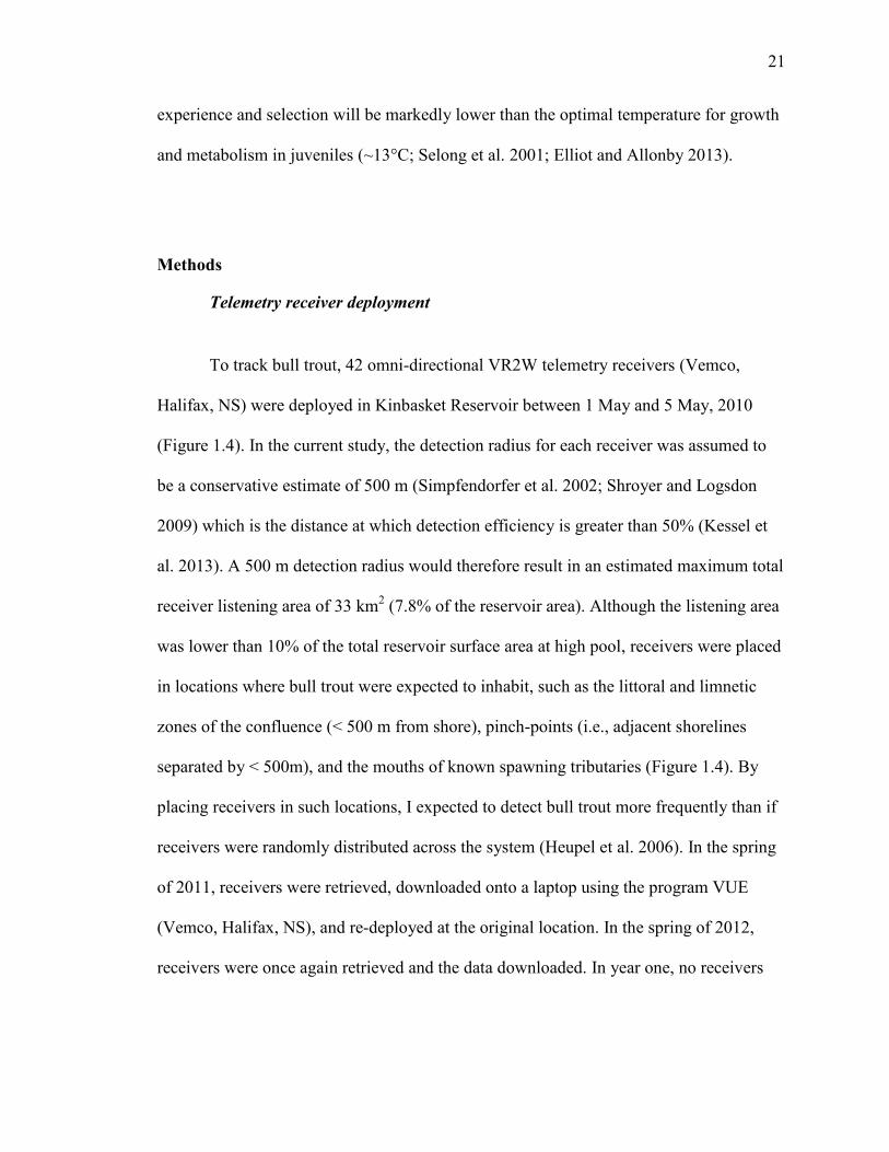
Telemetry receiver deployment

To track bull trout, 42 omni-directional VR2W telemetry receivers (Vemco,

Halifax, NS) were deployed in Kinbasket Reservoir between 1 May and 5 May, 2010

(Figure 1.4). In the current study, the detection radius for each receiver was assumed to

be a conservative estimate of 500 m (Simpfendorfer et al. 2002; Shroyer and Logsdon

2009) which is the distance at which detection efficiency is greater than 50% (Kessel et

al. 2013). A 500 m detection radius would therefore result in an estimated maximum total

receiver listening area of 33 km2 (7.8% of the reservoir area). Although the listening area

was lower than 10% of the total reservoir surface area at high pool, receivers were placed

in locations where bull trout were expected to inhabit, such as the littoral and limnetic

zones of the confluence (< 500 m from shore), pinch-points (i.e., adjacent shorelines

separated by < 500m), and the mouths of known spawning tributaries (Figure 1.4). By

placing receivers in such locations, I expected to detect bull trout more frequently than if

receivers were randomly distributed across the system (Heupel et al. 2006). In the spring

of 2011, receivers were retrieved, downloaded onto a laptop using the program VUE

(Vemco, Halifax, NS), and re-deployed at the original location. In the spring of 2012,

receivers were once again retrieved and the data downloaded. In year one, no receivers

22

were lost. In year two, five of the 42 receivers were lost, likely due to unusually low

water levels and spring-time ice movement.

Water temperature

Because the reservoir develops a thermal gradient for a short period of the year

(i.e., summer and fall) and maintains a steady surface elevation at the same time (Bray

2012), I focused the analysis of thermal habitat selection during this period which was

found to occur between approximately 9 August and 24 October, 2010. During low pool

in the spring of 2010, I deployed tidbit v2 thermister temperature loggers (Onset Hobo

Data Loggers - UTBI-001, accuracy ± 0.2°C, Bourne, MA) at two locations where water

temperatures were not affected by dam operations (Robertson et al. 2011), including in

the Columbia Reach and Canoe Reach. Three thermister loggers were suspended at

approximately 30 m intervals on each of the two receiver anchor ropes that were placed

in pelagic habitat (> 500 m from shore, e.g., Figure 1.3) with one additional logger

secured on shore where high pool water levels were projected to reach (during summer).

Data were collected at 1 hour intervals and converted into daily averages from August to

November, 2010. Loggers were retrieved the following spring when reservoir elevations

facilitated their recovery. Several thermal loggers failed to collect data from the Canoe

Reach, thus only temperature data from the Columbia Reach were used for the analysis of

thermal habitat selection (Figure 1.4).

Tagging

23

Adfluvial bull trout were sampled from 11 April to 25 May, 2010 by trolling near

the water surface (n = 122, Gutowsky et al. 2011). In summer, bull trout were captured by

angling at the mouths of known spawning tributaries (18 August to 9 September, 2010)

where fish congregate prior to spawning (n = 65). Upon capture, fish were placed in a

100 L cooler filled with lake water that was regularly replaced. Prior to surgery,

individual bull trout were then moved into another 100 L cooler that contained anesthetic

(40 mg/L; 1 part clove oil emulsified in 9 parts ethanol). Once anesthetized (characterized

by a loss of equilibrium and no response to squeezing the caudal peduncle), bull trout

were inverted and placed on a surgery table where a continuous supply of fresh water was

pumped through the mouth and across the gills. Total length (nearest mm) was measured

prior to surgery. For telemetry tag insertion and sex determination, a 3 cm long incision

was made posterior to the pelvic girdle along the midline of the fish following the

methods described by Wagner et al. (2011). Sex was determined by internal gonad

examination (males: small clear to white gonads; females: yellowish gonads containing

small to large eggs). A coded acoustic transmitter (model V13 TP; temperature data

transmissions every 2-6 minutes, accuracy ± 0.5°C) was inserted into the body cavity.

Incisions were closed using three simple interrupted stitches using 3/0 PDS-II absorbable

suture material (Ethicon Inc., Somerville, New Jersey). Prior to release, post-surgery fish

were allowed to fully recover in a bath of fresh water for ~30 minutes.

Tag temperature does not instantaneously reach equilibrium with the external

temperature (Negus and Bergstedt 2012). There is a latency time before the deep tissues

of fish reach thermal equilibrium with the ambient temperature, e.g., it can take 20

24

minutes for internal temperature to reach within 2°C of ambient temperature when fish

are exposed to a 15°C temperature change (Negus and Bergstedt 2012). Although bull

trout could swim between cooler and warmer temperatures without a detectable change in

core temperature, data in the current study were examined at a relatively course scale

(i.e., diel period) and therefore assumed representative of the average temperature

experience or selection for a given individual.

Data management and filtering

Temperature experience

Biotelemetry data from tagged bull trout were first filtered to remove false

detections and incomplete tag-to-receiver transmissions. The minimum number of

receiver detections per individual bull trout was set at two per receiver per 24 hour

period. Because surgical procedures were expected to affect behaviour for a short time

following surgery (Rogers and White 2007), analyses were only carried out on data

collected 7 days after tagging. The analysis only included detections that were recorded

after the final receiver was deployed in May, 2010. For the analysis of temperature

experience across two years, I calculated the average temperature recorded for each

fish/receiver/diel period (i.e., day/night). I arbitrarily selected a minimum of ≥ 20

detections/receiver to calculate the average temperature per diel period and individual.

Filtering ensured that transmitter detections were fish rather than code collisions or

environmental noise (summarized in Niezgoda et al. 2002) and decreased the total

number of observations, gathered across two years, to a reasonable number for statistical

25

analysis. Paired covariates included diel period (based on local sunset and sunrise times),

size (total length in mm), and sex. Data filtering and exploration were performed using

Microsoft Access and the R statistical environment (R Development Core Team 2012).

Thermal resource selection

Available thermal habitat was assessed during summer and fall by first generating

a line of best fit (3rd

-order polynomial, Parker et al. 1975) through the daily average

temperature collected by each thermal logger on the receiver rope in the Columbia Reach

(Figure 1.4). Based on the coefficients from each line of best fit, I estimated the

temperature (integers at 1°C intervals) at water depth , calculated the difference in water

depths for 2°C intervals, and converted these intervals into approximate percent of

available thermal habitat (see Appendix). Since there were only four thermal loggers for a

large volume of water, not all temperature profiles could be fitted with a 3rd

-order

polynomial. Nevertheless, I was able to estimate the vertical distribution of temperature

for 32 days between 9 August and 24 October, 2010.

Data were categorized into temperature bins of 2°C and counted as the number of

detections in a given bin per day (i) per individual (j) per habitat (k). Resource selection

was first assessed by examining whether an animal was found to use (1 = used, 0 = not

used) a given thermal habitat per day:

26

Where wijk is the selection index on the ith

day for the jth

individual for the kth

habitat, oijk is habitat use (1, 0), and lij is the proportion of available thermal habitat on the

ith

day. Indices can theoretically range between 0 and ∞.

To generate standardized resource selection indices, I first calculated wfijk as a

function of time spent at each thermal habitat such that a count of one detection was

equal to approximately two minutes (given the shortest possible tag transmission

interval). This allowed me to estimate the proportion of time spent in a given habitat

relevant to the total amount of time spent in that habitat on the ith

day by the jth

individual

for the kth

habitat. Based on the detection frequency (wfijk), I generated a standardized

selection index for each individual per day as:

∑

⁄

Where Bijk is the standardized selection index on the ith

day for the jth

individual

for the kth

habitat. Values of Bijk are constrained between zero and one where 1 represent

complete selection for a given temperature category on the ith

day and values close to 0

represent no selection.

Analyses


27

Temperature experience of the bull trout population was modelled across two

years using a generalized additive mixed-effects model (GAMM, Zuur et al. 2014). I used

Akaike Information Criteria to select the most parsimonious model from a set of

candidate models (Akaike 1974). The model for temperature experience contained the

number of days since beginning the study (continuous variable: day of the year since

January 1, 2010, abbreviate as “day”) as a smoother (Wood 2006, 2011) and fish ID as a

random factor. Candidate models (n = 18) contained one or more combinations of

covariates, including: sex, body size, diel period (day or night, based on sunset and

sunrise data), and a number of two-way interactions (Table 2.2). Models were estimated

using restricted maximum likelihood and error terms were assumed to follow a gamma

distribution to ensure fitted values were strictly positive. Models were fitted to the data

using the R packages “nlme” (Pinheiro et al. 2013) and “mgcv” (Wood 2006, 2011). I

validated the final models by examining for patterns in the normalized residuals and by

examining residual lag plots (Zuur et al. 2009). Despite the inclusion of random effects,

the model validation process identified residual autocorrelation. Models were therefore

further fitted with continuous autoregressive correlation structure on individual animals

(Zuur et al. 2009). Including a correlation structure and random effect allowed me to

model compound correlation between observations from the same animal and the

temporal correlation between all observations from the same animal and the irregularly

spaced number of days between observations since beginning the study (Zuur et al.

2009). Further model validation showed no significant residual autocorrelation. Finally,

plotting the Pearson residuals at each receiver coordinate indicated a random distribution

and therefore no clear evidence for spatial autocorrelation (Zuur et al. 2009).

28


I based the model of thermal resource selection on several recommendations from

the literature: 1) time must be included as the dimensional unit with which to quantify the

thermal environment as a resource (Roughgarden et al. 1981; Tracy and Christian 1986;

Dunham et al. 1989); 2) thermal availability is allowed to change with time (Arthur et al.

1996) and; 3) when individual is the level of replication, individual must be included as a

random factor (Gillies et al. 2006). Similar to the analysis of thermal experience, thermal

resource selection was modelled using a GAMM with animal ID as a random factor.

Given that initial data exploration indicated an abundance of zeros (87%, indicating no

use of a given thermal resource) for an analysis that included both selected and non-

selected thermal resource, I instead only analysed selection for thermal resources that

were experienced by bull trout. Although selection should be based on the range of

thermal habitats that were available (Tracy and Christian 1986; Bakken 1989: from Hertz

1992), models would not converge with such zero-inflation. Only unstandardized

selection indices (wijk) were examined across all available thermal habitats. Since there

was a small number of data available (n = 32), I only ran a simple model that included a

smoother for day of the year (by each thermal resource) and thermal habitat as a

categorical predictor. No model selection was performed. The intercept was allowed to

randomly vary for each individual fish. The response variable used was wijk. Although

wijk can theoretically vary between 0 and ∞, values of wijk during the current study varied

between 1.81 and 16.91. Due to serial autocorrelation, I included a CAR1 correlation

structure to model the dependency between residuals at different time points (Zuur et al.

29

2009). The model was estimated using restricted maximum likelihood and the error term

was assumed to follow a Gaussian distribution. The model of habitat selection was

assessed using the techniques described by Zuur et al. (2009). No serial autocorrelation

was observed after incorporating the correlation structure.

Results

After filtering the raw data, 17 422 temperature observations were available to

analyse the average temperature experience from 151 individuals (81% of tagged bull

trout). Males outnumbered females approximately 2:1 and the average size of males and

females was similar at 612 mm TL ± 91 SD and 622 mm TL ± 66 SD. Males contributed

only slightly more data (~55%) than females (~45%). For the analysis of thermal

resource selection, there was a high degree of variation within temperature categories and

availability of the upper most categories decreased with time (Figure 2.1). From 9 August

to 24 October 2010, bull trout experienced temperatures between 9°C and 15°C.

However, only one individual was detected in the temperature category of 9-11°C (once

in September) and was therefore removed from the analysis. The model of thermal

habitat selection therefore contained only two temperature categories (11-13°C and 13-

15°C) for which to examine how bull trout selected their thermal environment over time.


30

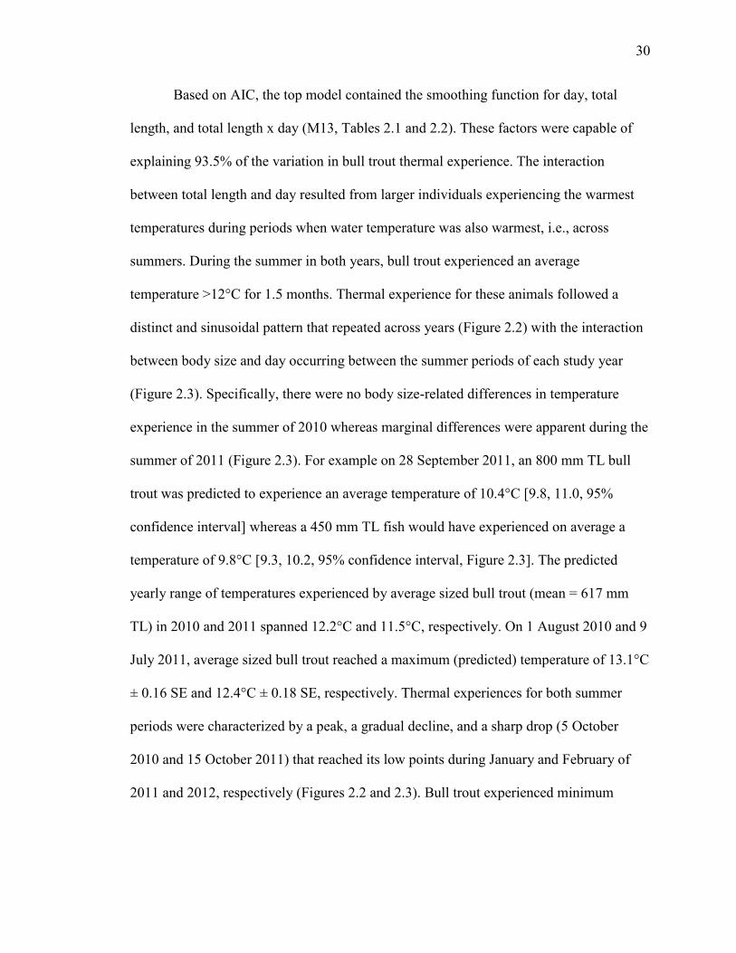
Based on AIC, the top model contained the smoothing function for day, total

length, and total length x day (M13, Tables 2.1 and 2.2). These factors were capable of

explaining 93.5% of the variation in bull trout thermal experience. The interaction

between total length and day resulted from larger individuals experiencing the warmest

temperatures during periods when water temperature was also warmest, i.e., across

summers. During the summer in both years, bull trout experienced an average

temperature >12°C for 1.5 months. Thermal experience for these animals followed a

distinct and sinusoidal pattern that repeated across years (Figure 2.2) with the interaction

between body size and day occurring between the summer periods of each study year

(Figure 2.3). Specifically, there were no body size-related differences in temperature

experience in the summer of 2010 whereas marginal differences were apparent during the

summer of 2011 (Figure 2.3). For example on 28 September 2011, an 800 mm TL bull

trout was predicted to experience an average temperature of 10.4°C [9.8, 11.0, 95%

confidence interval] whereas a 450 mm TL fish would have experienced on average a

temperature of 9.8°C [9.3, 10.2, 95% confidence interval, Figure 2.3]. The predicted

yearly range of temperatures experienced by average sized bull trout (mean = 617 mm

TL) in 2010 and 2011 spanned 12.2°C and 11.5°C, respectively. On 1 August 2010 and 9

July 2011, average sized bull trout reached a maximum (predicted) temperature of 13.1°C

± 0.16 SE and 12.4°C ± 0.18 SE, respectively. Thermal experiences for both summer

periods were characterized by a peak, a gradual decline, and a sharp drop (5 October

2010 and 15 October 2011) that reached its low points during January and February of

2011 and 2012, respectively (Figures 2.2 and 2.3). Bull trout experienced minimum

31

temperatures between 1°C and 2°C from January to April in 2010 and slightly warmer

minimum temperatures from January to April in 2011.


In the model of thermal resource selection, smoothers for both 11-13°C and 13-

15°C were highly significant (Table 1). Smoothers explained 60.5% of the variation in wij

(adjusted R2). Bull trout selected temperatures between 11°C and 13°C as availability

first decreased and later increased in late September and October (Figure 2.3).

Simultaneously, availability of warmer temperatures (13-15°C) decreased as bull trout

continued to select for these temperatures (Figures 2.1 and 2.3). The standardized

selection index (Bij), which included all temperature categories recorded during the

period from 9 August to 24 October 2010 (n = 505) and is here calculated as an average

across all fish and days, indicated that temperatures between 11-13°C were selected 1.6

times and 31 times more often than temperatures between 13-15°C and 9-11°C,

respectively. Despite their availability during the summer to fall period, temperature

categories below 9°C and those above 15°C were never selected on any of the days where

thermal resource availability data were calculated (Figures 2.3 and 2.4; Table 2.3).

Discussion

In addition to experiencing a narrow range of temperatures that were clearly

related to season (H1, Figure 2.2), adfluvial bull trout selected a small range of

32

temperature (11 to 15°C) during the period of weak thermal stratification and when

additional ambient temperatures are available in the water column. Although this species

has been shown to occupy a range of temperatures (Howell et al. 2010) and I do not

suggest bull trout never venture into warmer or cooler water, in Kinbasket Reservoir a

large number individuals showed a remarkably narrow thermal experience across two full

years (Figure 2.2). The average temperature experience was between 12°C and 13°C for

1.5 months in both years when warmer and cooler temperatures were available, perhaps

indicating temperature preference in wild bull trout. Maximum temperatures were

experienced during the peak of summer and minimums during a period when much of

system is covered in ice (Figure 2.3). Notably, thermal experience remained within a

narrow window during the period of weak stratification (when the greatest range of

temperatures would be available) and outside this period when temperatures would be

isothermal (Bray 2012). Indeed, confidence limit width may reflect the variability of

thermal habitat whereas mean estimates and the temperature selection analysis indicates

temperature preference as these animal swam freely in the system (Figure 2.3).

Theoretically, ectotherms should select temperatures that deliver physiologically

optimal conditions (Tracy and Christian 1986, Wildhaber and Crowder 1990, Sims et al.

2004). Adfluvial bull trout were expected to show a relationship between body size and

temperature such that larger individuals should experience, on average, colder

temperatures than smaller conspecifics (Morita et al. 2010a; Jonsson and Jonsson 2011;

Elliot and Allonby 2013). Laboratory experiments have rather consistently demonstrated

this relationship in young fish (e.g., age 0+ - 3+; Coutant 1997; Mccauley and Huggins

1979; Morita et al. 2010b; Elliot and Allonby 2013). However, for larger (i.e., adult)

33

specimens examined in the field, the relationship is not always as clear. Spigarelli et al.

(1983) found that while the upper preferred temperature for large wild riverine brown

trout was 1.5°C lower than the reported final preferendum for juveniles, body size was

not a significant covariate to explain central tendency of temperature experience. In the

current study, the average temperature for a large adfluvial bull trout remained below the

optimal temperature for juveniles and slightly above the average temperature experienced

by a conspecific of roughly half the size (Figure 2.3). Despite laboratory findings and

some field-based research, according to Jonsson and Jonsson (2011), there may be no

direct relationship between either the optimum temperature for growth or the temperature

for maximum growth efficiency and habitat selection by wild salmonids. In nature,

resource selection involves a complex suite of factors that may weight differently

according to a number of variables (e.g., phenotypic traits, environmental conditions) as

it does with diel vertical migration (Busch and Mehner et al. 2012). In Kinbasket

Reservoir, preferred temperatures may not be limiting, as the gradual thermocline covers

a wide range of temperatures across a range of depths (Bray 2011, 2012). Thus, smaller

individuals can maintain their preferred temperatures while remaining at deeper depths

than larger cannibalistic conspecifics (Beauchamp and Van Tessel 2001; In Chapter 3).

Again, in nature the relationships between temperature preference and body size may not

be as straightforward as in the laboratory (Jonsson and Jonsson 2011).

Bull trout occupied a narrow range of temperatures that changed with availability

when the reservoir contained a thermal gradient (H2, Figure 2.4). Behavioral

thermoregulation, which occurs when ectothermic animals actively maintain their body

34

temperature close to a defined target range where performance is maximized (Huey 1982;

Hertz et al. 1993; Diaz and Cabezas-Diaz 2004), is an important component of resource

selection in ectotherms (Cowles and Bogert 1944; Magnuson and Crowder 1979; Huey

1991; Reinert 1993). Analogous to terrestrial lizards that thermoregulate by moving

across different elevations (Hertz and Huey 1981; Adolph 1990), fishes exhibit

behavioural thermoregulation across depth gradients in pelagic habitat (Brett 1971;

Cartamil and Lowe; Jensen et al. 2006; Sims et al. 2006). Although thermal resource

availability along a vertical gradient is certainly not the only factor to consider when

assessing habitat selection (Plumb and Blanchfield 2009), two biologically reasonable

outcomes remain evident from the results of the current study. First, excluding the single

detection between 9-11°C, bull trout occupied only a relatively narrow window of

temperatures between 11 and 15°C that accounted for 41.6% of the available temperature

range from August to October, 2010 (H2, Table 2.3). Second, bull trout selected these

temperatures as availability fluctuated for the coolest temperature category (11-13°C) and

significantly decreased for the warmest category 13-15°C (H2, Figure 2.4). Given that fish

can detect relatively fine-scale changes in temperature (Brett 1971) and variables such as

wind, cloud cover, and rain will alter thermal resource availability on a daily basis

(Wetzel 2001), aquatic ectotherms ought to respond to daily changes in available thermal

resources while simultaneously accounting for additional abiotic and biotic factors. As

metabolically optimal water temperatures decrease in availability with the progression of

autumn, bull trout continue to select for these diminishing thermal resources (Figure 2.4).

35

While there may be a bioenergetic advantage to selecting a small range of

temperatures within a changing volume of thermal habitat, there are also costs associated

with selection, for example a trade-off with the likelihood of encountering prey

(Scheuerell and Schindler 2003). Behaviour is expected to vary spatially and temporally

as a result of trade-offs, e.g., thermal preference may be conditional on availability or the

presence of prey, predators, and competitors (Mysterud and Ims 1998; Downes 2001,

Godvik et al. 2009). For example, Downes (2001) found that garden skinks

(Lampropholis guichenoti) basked relatively infrequently in the presence of predator

scent, indicating a trade-off for safety over growth, size at maturity, and clutch mass later

in life. In the current study, the small sample size for thermal resource selection did not

permit the inclusion of additional variables that may identify trade-offs such as those

documented in diel vertically migrating organisms (Mehner 2012). Scheuerell and

Schindler (2003) provided evidence to suggest that juvenile sockeye minimized the ratio

of predation risk to foraging gain while performing diel vertical migration. In Kinbasket

Reservoir, optimal temperatures and adequate dissolved oxygen concentrations (>8

mg/L) is apparently not limiting across depths (Bray 2011, 2012; Chapter 3). Bull trout

diel vertical migration was hypothesized to result from trade-offs among feeding

opportunities, bioenergetics, and predator avoidance (Mehner 2012; Chapter 3), however

DVM appears to occur more of a result of diel period rather than temperature, i.e., DVM

occurs across a range of temperatures that change little during any given 24 hour period.

Given that temperature experience but not depth distribution is the same for large and

small bull trout, it follows that smaller individuals are occupying deeper darker water as

refuge from conspecific predators that are known for cannibalism under high population

36

densities (Wilhelm et al. 1999; Beauchamp and Van Tassell 2001; Chapter 3). Although

their density has not been measured, bull trout are considered abundant in Kinbasket

Reservoir (Gutowsky et al. 2011). While the current study presents evidence of thermal

resource selection across a thermal gradient, further research should determine how trade-

offs influence this apparent selection, e.g., the inclusion of additional covariates such as

diel period and body size (Mysterud and Ims 1998; Godvik et al. 2009).

Temperature is commonly used by governments to define habitat suitability for

both freshwater and marine fish species (Rosenfeld and Hatfield 2006; Bear et al. 2007;

Cheung et al. 2010). As global temperatures continue to rise, shifting thermal regimes

and climate patterns are affecting fish behaviour, physiology, and life history (Walther et

al. 2002; Munday et al. 2008; Robinson et al. 2009). While it is important to model

potential changes in thermal resource availability, the long-term physiological and

behavioural impacts of increased temperature requires further investigation in free-

ranging fish (Plumb and Blanchfield 2009; Elliot and Elliot 2010; Coutant 2012),

particularly given the apparent sensitivity and selectivity of threatened species such as

bull trout. Although climate and habitat simulation models are useful tools to project

habitat suitability (e.g., Jones et al. 2013), there is real value in acquiring temperature

data from wild animals (Cooke et al. 2004). In the current study, adfluvial bull trout

exhibited a narrow thermal experience across two years and showed selection for

temperatures between approximately 13-15°C during a period when the system contained

a thermal gradient (Figure 2.3). Combined with temperature experience data, similar but

longer-term investigations could illustrate how bull trout and other thermally sensitive

37

species modify their behavioural in response to their environment, including climate-

driven changes in the available thermal regime. It may be unclear exactly how a warming

climate will affect the amount of available thermal habitat for cold-water fish (In Plumb

and Banchfield 2009); however, climate change will almost certainly influence

behavioural thermoregulation (Casselman 2002; Coutant 2012, Wenger et al. 2013).

Given that temperature is a resource for pelagic fish and habitat characterization is

critical to the successful management of species at risk (Rosenfeld and Hatfeld 2006),

free-ranging thermally sensitive fish would be exceptional tools to both identify critical

thermal habitat and show how it changes as the climate warms.

Two years of telemetry data illustrated a narrow temperature experience and

thermal resource selection in a cold-water stenotherm. Contrary to my hypothesis, there

was no appreciable effect of body size on temperature experience in adfluvial bull trout.

These results require further investigation, for instance at finer temporal scales and in

relation to additional abiotic and biotic covariates (e.g., the presence of predators and

prey). While numerous studies have identified the importance of temperature on fish

behaviour and metabolism, resource selection has only rarely been examined in fishes

across different thermal regimes (Plumb and Blanchfield 2009; Pierce et al. 2013; Goyer

et al. 2014). Although not all fishes will be equally affected by climate warming (Somero

2010), many will experience behavioral modifications and physiological impairments

resulting from changes to environmental variables such as oxygen and temperature

(Pörtner and Knust 2007; Coutant 2012). Thermal experience and thermal resource

selection are particularly useful tools for identifying how thermally sensitive and already

38

threatened species might react to climate change. Based on these findings, longer-term

field-based data collection on thermal resource selection in thermally sensitive species is

a suitable method for projecting the impacts of climate change on cold-water fishes.

39

Tables

Table 2.1- Model output for the generalized additive mixed models of temperature

experience (1) and thermal habitat selection (2). Test statistics are given from the F-

distribution for the GAMM component and t-distribution for the linear-mixed effects

components of the model. Random intercept variance in model 1 was 0.21 for fish ID.

Random intercept variance for model 2 was 0.35 for fish ID. Values of autocorrelation at

lag 1 (φ) for models 1 and 2 were 0.914 and 0.13, respectively.

Model # response parameter DF test statistic P-value

1. Temperature

(°C) s(Day) 9.0 F = 10938 < 0.0001

TL 149 t = -0.676 0.500

TL:Day 17269 t = 2.38 0.017

2. wij s(Day of year):

11-13°C 3.24 F = 14.71 < 0.0001

s(Day of year):

13-15°C 1.00 F = 16.50 < 0.001

Temperature

Category 1.00 t = 5.53 < 0.0001

40

Table 2.2- The set of candidate models used to test temperature experience by bull trout across two years (2010-2012). The

number of parameters is given by K.

Model

Name Model K AIC

M13 y = s(DAY) + TL + TL:DAY 8 16906.6

M16 y = s(DAY) + TL + SEX + TL:Day 9 16909.1

M14 y = s(DAY) + SEX + TL:Day 8 16912.1

M11 y = s(DAY) + TL 7 16914.9

M17 y = s(DAY) 6 16916.5

M7 y = s(DAY) + SEX + TL 8 16917.1

M10 y = s(DAY) + SEX 7 16919.2

M0 y = s(DAY) + SEX + TL + DIEL + TL:DAY + DAY:SEX + TL:DIEL 12 16921.2

M2 y = s(DAY) + SEX + TL + DIEL + TL:DAY + TL:DIEL 11 16924.1

M1 y = s(DAY) + SEX + TL + DIEL + TL:DAY + DAY:SEX 11 16924.8

M4 y = s(DAY) + SEX + TL + DIEL + TL:DAY 10 16927.7

M15 y = s(DAY) + DIEL + TL:DAY 8 16928.1

M5 y = s(DAY) + SEX + TL + DIEL + TL:DIEL 10 16932.7

M9 y = s(DAY) + TL+ DIEL 8 16933.6

M12 y = s(DAY) + DIEL 7 16935.3

M8 y = s(DAY) + SEX + DIEL 8 16938.1

M3 y = s(DAY) + SEX + TL + DIEL + DAY:SEX + TL:DIEL NA

failed to

converge

M6 y = s(DAY) + SEX + TL + DIEL + DAY:SEX NA

failed to

converge

41

Table 2.3- Standardized selection index (Bij) and average available thermal habitat (%) in each temperature category. Bij was

calculated for individual fish (j) per day (i) and taken simply as the mean during the study period from 9 August – 24 October,

2010.

Temperature

Category (°C)

Mean Bij

SD Bij - 95%

CI

+ 95%

CI

n Zeros

(n)

%

Avail

SD

5-7 0 0 NA NA 121 121 30.73 5.37

7-9 0 0 NA NA 121 121 12.76 7.73

9-11 0.008 0.088 NA NA 121 120 12.78 7.12

11-13 0.5014 0.4564 0.415 0.588 107 38 25.95 14.15

13-15 0.3162 0.4104 0.169 0.463 30 14 15.65 15.02

15-17 0 0 NA NA 5 5 2.13 5.46

42

Figures

Figure 2.1 - Temperature availability (%) for each thermal category (e.g., 5-7°C) between 9 August and 24, October, 2010.

Lines of best fit (± 95% confidence limits) are shown to illustrate trends in availability.

43

Figure 2.2 - The smoother and 95% point-wise confidence limits from the top model to predict daily bull trout thermal

experience across years (2010-2012). The smoother is highly significant (F = 13388, P < 0.0001) and illustrates seasonal

changes across both years. Degrees of freedom are taken from the model hat matrix and given parenthetically in the y-axis.

Days since January 1, 2010

44

Figure 2.3 - The predicted values (± 95% confidence limits) for bull trout temperature experience in Kinbasket Reservoir from

21 June 2010 to 10 March 2012. The x-axis is days since January 1, 2010. The temperature experience large fish (800 mm TL)

are shown as a solid line demarcated by circles whereas small fish (400 mm TL) are shown with a dashed line demarcated by

squares. The approximate timing of astronomical seasons is illustrated with vertical dashed lines.

0

2

4

6

8

10

12

14

Tem

per

atu

re (

°C ±

95

% C

I)

Days since January 1, 2010

Summer

solstice

Autumnal

equinox

Summer

solstice

Winter

equinox

Vernal

equinox

Autumnal

equinox

Winter

equinox

200 400 600 800

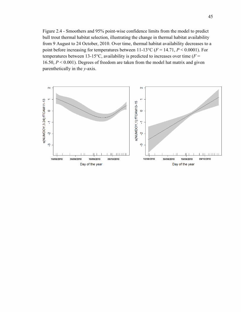
45

Figure 2.4 - Smoothers and 95% point-wise confidence limits from the model to predict

bull trout thermal habitat selection, illustrating the change in thermal habitat availability

from 9 August to 24 October, 2010. Over time, thermal habitat availability decreases to a

point before increasing for temperatures between 11-13°C (F = 14.71, P < 0.0001). For

temperatures between 13-15°C, availability is predicted to increases over time (F =

16.50, P < 0.001). Degrees of freedom are taken from the model hat matrix and given

parenthetically in the y-axis.

46

Chapter 3: Diel vertical migration hypotheses explain size-dependent behaviour in

bull trout

Abstract

In aquatic organisms, DVM is typically characterized as ascent at dusk and descent at

dawn. Often several hypotheses are required to explain the sensory-mechanisms and

ultimate causes of DVM. Currently, most of the research focused at the individual level

has identified DVM functions as a response to light, feeding opportunities, predator

avoidance, and bioenergetics in small planktivores. However, there are no studies

examining whether DVM hypotheses can explain and predict individual behavioural

characteristics in top-level predators. In this study, I hypothesized that bull trout, a cold-

water pelagic-cruising piscivore, will exhibit size-dependent, daily, and seasonal patterns

in DVM that are consistent with light levels (proximate trigger) and the feeding

opportunities, predator avoidance, and bioenergetics hypotheses. To test these

hypotheses, depth-sensing acoustic transmitters were implanted into 187 bull trout (358 -

881 mm total length) that were free-swimming for one year in Kinbasket Reservoir. I

found that bull trout were shallowest at night, deepest during the day, and exhibited clear

patterns of DVM across all seasons. In line with the predator avoidance hypothesis, large

and small bull trout occupied different depths in all seasons except the spring, while the

likelihood of depth change for large and small fish varied depending on season and diel

period. The greatest depth difference among large and small bull trout occurred in the

summer and less-so in autumn. In the summer, small bull trout remained at greater

average depths (~ 15 m) than larger fish (~7 m) regardless of diel period. The results of

47

this study indicate light as a proximate trigger and since there is no clear temperature-

related bioenergetic advantage to changing depths during winter, feeding opportunities

and predator avoidance are the most parsimonious DVM hypotheses to explain body-size

dependent behaviour in this top-level predator.

48

Introduction

In fishes, DVM is a behaviour that is typically characterized as ascent at dusk and

descent at dawn (Neilson and Perry 1990). Linked to a number of processes including

thermoregulation (Brill et al. 1999; Cartamil and Lowe 2004; Sims et al. 2006), habitat

selection (Pade et al. 2009; Plumb and Blanchfield 2009), and foraging (Sims et al. 2005;

Fox and Bellwood 2011), the functional triggers and adaptive drivers of DVM currently

explain patterns across daily and seasonal periods for planktivorous fish populations only

(e.g., Bevelhimer and Adams 2003; Gjelland et al. 2009; Quinn et al. 2012). Although

piscivores have been hypothesized to exhibit DVM in relation to prey species (Jensen et

al. 2006; Kahilainen et al. 2009), investigations of depth and vertical movement in

relation to the mechanisms (e.g., size-dependent behavior) thought to be responsible for

DVM remains scant and there are no studies on individual DVM patterns in piscivorous

fish.

Recently DVM has been related to both proximate triggers (i.e., sensory-motor

and genetic developmental mechanisms) and ultimate causes (i.e., behaviours shaped by

natural selection) (Mehner 2012). Proximate triggers include changes in light intensity

and, to a lesser extent, changes in hydrostatic pressure and responses to thermal gradients

(Levy 1990; Mehner 2012). Ultimate causes of DVM are hypothesized to be related to

bioenergetic efficiency, feeding opportunities, and predator avoidance behaviour (Mehner

2012). Evidence to support these hypotheses, whether functional or adaptive, is often

generated from observational studies which are the most appropriate means of obtaining

49

such information on migratory behavior in free-living animals. For example, Levy (1990)

used hydroacoustic sonar to infer that patterns of DVM in juvenile sockeye salmon

(Oncorhynchus nerka) were related to changes in light and thermoregulation. In fishes,

the most pervasive mechanism thought to reflect predator avoidance behaviour and prey

detection is individual body size. Again using hydroacoustics, small planktivorous fish

were shown to be either deeper (Levy 1991) or ascend earlier and descend later (Busch

and Mehner 2012) compared with large-sized conspecifics.

In this study I test DVM hypotheses across a wide size range (358 to 881 mm TL)

of adfluvial bull trout (Salvelinus confluentus) in Kinbasket Reservoir (Figure 1.4).

Adfluvial bull trout are an excellent candidate species because they: 1) possess a low

thermal tolerance (Selong et al. 2001); 2) primarily feed on vertically migrating kokanee

salmon (Levy 1991, Bevelhimer and Adams 1993); 3) exhibit intra- and interspecific

competitive behaviour (Beauchamp and Van Tassell 2001; Stewart et al. 2007); and iv)

are similar to other cold-water pelagic-cruising predators [e.g., coaster brook charr

(Salvelinus fontinalis), lake charr (Salvelinus namaycush)]. Although not studied in

Kinbasket Reservoir, it is well established that kokanee salmon may perform DVM in

part to prey on cladocerans that also perform DVM (Bevelhimer and Adams 1993;

Ringelberg 1999). Biotelemetry data were used to test hypotheses about DVM in bull

trout over an entire year. I hypothesized that putative factors related to DVM including

diel period (proximate trigger), season (temperature-related bioenergetics efficiency), and

body-size (feeding opportunities and predator avoidance) would give rise to predictable

patterns in depth distribution and vertical movement. Following the patterns observed in

50

other salmonids (e.g., Levy et al. 1990), I predicted that individuals would be shallowest

at night. Since bull trout are a cold-water species (Selong et al. 2001) and the reservoir

develops a thermal gradient (Bray 2012), bull trout were predicted to be deepest in the

summer and shallowest in the winter and spring. While it was not possible to directly test

individual interactions, any size-dependent depth distributions and vertical movements

were predicted to result from competition and cannibalism risk among bull trout

(Beauchamp and Van Tassell 2001).

Methods

The study location is described in Chapter 1 (Figure 1.4). In addition, VR2W

deployment, retrieval, and fish tagging followed similar procedures to those outlined in

Chapter 2. Testing my hypotheses for size-dependent DVM across seasons required only

a single year of data, thus only data from 2010 – 2011 were analyzed.

Database Management and Analysis

Biotelemetry data were sorted and stored in a Microsoft Access database. Bull

trout detections were considered for analysis after the final receiver was deployed on 5

May, 2010. As described in Chapter 2, detections that occurred within one week

following tagging of a particular fish were excluded from the analysis.

51

Seasons were delineated as: winter (January to March), spring (April to June),

summer (July to September), and autumn (October to December). The autumn

represented the reproductive period between the first observation of bull trout traversing

spawning tributary rapids (personal observation) to the end of the post-spawning period

and beginning of the coldest few months of the year (i.e., winter). Since it was impossible

to use traditional tools to measure diel patterns of light intensity (e.g., Secchi disk, Wetzel

2001), diel period was divided into day (> local sunrise and < local sunset) and night (>

sunset and < sunrise) for a given 24 hour period.

Patterns in DVM were assessed by examining the average depth and absolute

maximum change in depth (herein after referred to as vertical movement) by diel period,

season, and body size. For depth, detections were calculated as the average depth from a

minimum of 9 detections from each fish, per hour, and acoustic receiver ID (termed a

detection event). Such filtering ensured that transmitter detections represented fish rather

than code collisions or environmental noise (summarized in Niezgoda et al. 2002) while

also decreasing the total number of data points to reach model convergence in the R

statistical environment. In addition, filtering the data into hourly periods restricted the

maximum number of detections from each fish at each receiver to 19 (given the tag

transmission rate). Thus between 9 and 19 detections were used to calculate depth and

vertical movement for each filtered data point. Based on the time, date, and body size

measurement of each detection event, data were categorized into seasons, diel periods,

and hour of the day (for examining plots of the observed data). Vertical movement was

calculated as the detected absolute maximum change in depth during a detection event

52

and rounded to the nearest integer. Since only larger changes in depth were considered

biologically relevant, vertical movement was also assigned a “1” if movement was

detected (Δ depth ≥ 0.5 m) and “0” if movement was minimal or not detected (Δ depth <

0.5 m). To first check for continuous hourly patterns of vertical movement, plots of depth

and vertical movement from the filtered data were examined and fitted with smoothing

functions of the class cyclic penalized cubic regression spline (Wood 2000; Wood 2006).

Outliers from the filtered database were identified by examining Cleveland dot plots and

model residual plots (Zuur et al. 2009). Although the accuracy of all detections could not

be verified, outliers were documented as > 60 m when depth was the response variable.

The majority of recordings greater than 60 m were likely erroneous since this fish depth

was often greater than the actual water depth (measured by known reservoir elevation and

the receiver depth) at the time of detection. Therefore detections of > 60 m deep (n = 120,

< 0.01%) were removed from the analyses.

Model Type, Model Selection, and Model Validation

Depth distribution was modelled using a generalized linear mixed-effects model

(GLMM) that treated the response variable, fish depth, as a count (rounded to the nearest

integer), individual fish as a random factor (Pinheiro and Bates 2000), diel period and

season as fixed factors, and total length as a continuous covariate. The model of depth

distribution was used to answer the question: which of the putative factors are correlated

with bull trout depth distribution? Vertical activity was modeled to address two

questions: (i) which of the putative factors are associated with the likelihood that bull

53

trout change depth, and (ii) when bull trout change depth, which of the putative factors

are correlated with the magnitude of the depth change? To answer question (i), a binary

response variable (vertical movement = 1, no vertical movement = 0) was modeled as a

function of predictor variables (season, diel period, and body size), with individual fish as

a random factor. To answer question (ii), the magnitude of vertical activity was estimated

by subsetting the data (Δ depth ≥ 0.5 m) and treating the response as a count variable

(rounded to the nearest integer), individual fish as a random factor, diel period and season

as fixed-predictor variables, total length as a continuous covariate, and an offset variable

(log-elapsed time, Zuur et al. 2009) for the time between the shallowest and deepest

detections. The parameters of all models were estimated using penalized quasi-likelihood

(PQL, Bolker et al. 2009).

The best model was selected based on the number of factors that were highly

significant (p < 0.01) in the full models containing the available predictor variables and

two-way interactions (Zuur et al. 2009). The selection method was appropriate since

Akaike Information Criteria (AIC) scores are not widely available for GLMMs with PQL

estimation (Zuur et al. 2009) and because likelihood-based methods (e.g., AIC ranking)

are generally discouraged when using PQL estimation (Bolker et al. 2009). Two-way

interactions were considered as potentially biologically relevant, however three-way

interactions were not considered because they are often difficult to interpret, add

unnecessary complexity to models, and add little value to understanding the underlying

ecological relationships (Bolker et al. 2009; Zuur et al. 2009). Competitive interactions

between individuals could not be directly modelled given the limitations of the statistical

54

designs and biotelemetry equipment, however strong size-dependent effects on depth and

vertical movement were considered weak evidence for competitive interactions.

Autocorrelation was addressed by adding an autocorrelation moving-average correlation

structure to all models (corARMA, Pinheiro and Bates 2000). Q-Q plots and residual

plots were used to evaluate normality, heterocedasticity of residuals, and overdispersion

(models with Poisson response only). Spatial autocorrelation was checked by plotting the

size of the Pearson residuals at each receiver coordinate (Zuur et al. 2009). Residual size

was randomly distributed across receivers. An autocorrelation function (ACF) was used

to determine whether the moving-average correlation structure reduced autocorrelation

(Pinheiro et al. 2013). In all models the ACF plots showed the correlation structures to

reduce autocorrelation. Models were graphically validated following Pinheiro and Bates

(2000) and Zuur et al. (2009). Analyses and plots were done in R (version 2.15.3, R

Development Core Team 2012) using the packages MASS (Venables and Ripley 2002),

nlme (Pinheiro et al. 2013), and ggplot2 (Wickham 2009). Although highly significant P-

values were used to determine which model terms were retained, large degrees of

freedom warranted that effect sizes and a lack of confidence limit overlap be used to

indicate significant differences among groups.

Results

Filtering from the raw dataset (n = 1 309 115 detections) resulted in 27 372 depth

observations that were acquired from 171 fish (91% of tagged bull trout). Bull trout size

ranged from 358-881 mm TL and was well represented across diel periods and seasons

55

(Table 3.1). The observed data showed typical DVM patterns where bull trout descended

at dawn and ascended at dusk (Figure 3.1). This pattern was least pronounced in the

winter and spring and most pronounced in the summer and autumn (Figure 3.1). Vertical

activity appeared to increase at sunrise and decrease at sunset and was also observed to

vary across seasons (Figure 3.2).

To explain bull trout depth, the model containing all factors and two-way

interactions contained the greatest number of highly significant terms (Table 3.2, Figure

3.3). Bull trout were shallower during the night than in the day and depending on season,

small bull trout were estimated to be deeper than large bull trout (Figure 3.3). Results

from the model predictions indicated that fish between 480 mm and 640 mm (n = 72)

consistently showed significant differences in depth distribution between day and night

periods across seasons (Figure 3.3). During the winter, summer, and autumn, larger bull

trout tended to be shallower than smaller conspecifics. For example, a 400 mm bull trout

detected on a summer day was estimated to be at a depth of 15.3 m [12.9, 18.1, 95%

confidence interval] whereas a bull trout that was twice as long and detected during the

same period was estimated to be almost twice as shallow at 7.8 m [6.4, 9.4, 95%

confidence interval]. Overall, a typical bull trout (average TL= 590 mm TL) was deepest

during a summer day and shallowest during a winter or spring night (Figure 3.3).

To evaluate the probability that a bull trout changed depth during a detection

period, the most highly significant model contained all main effects and two-way

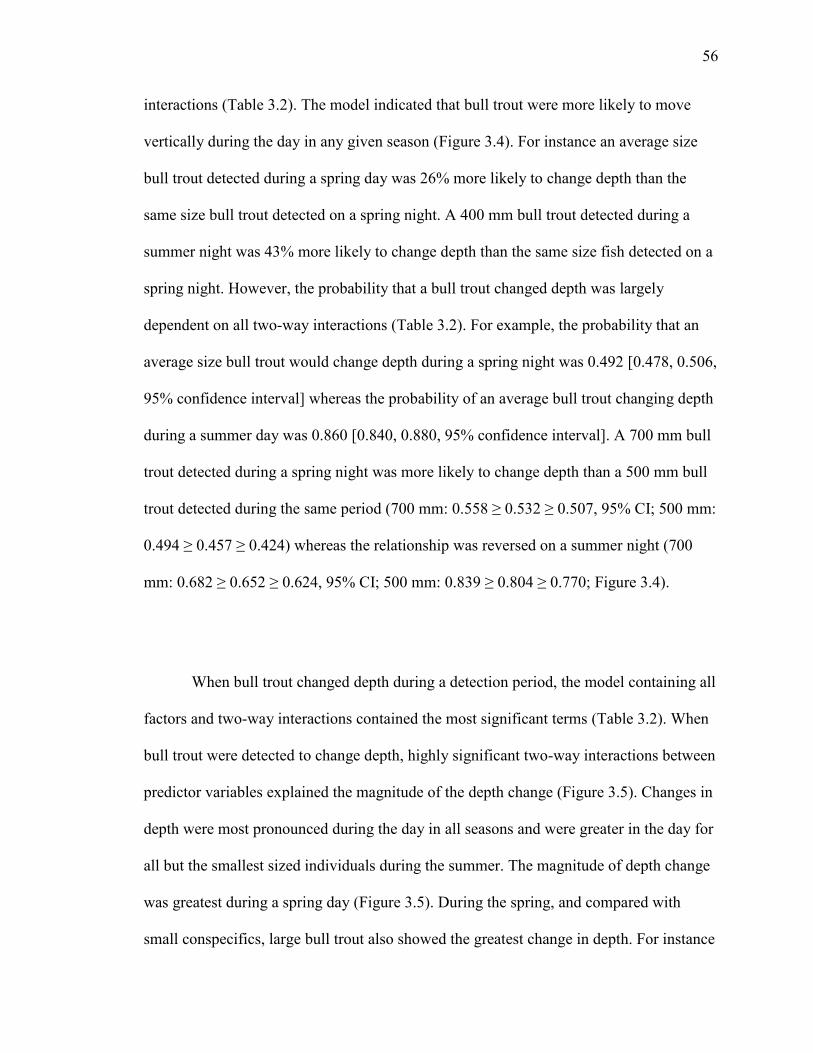
56

interactions (Table 3.2). The model indicated that bull trout were more likely to move

vertically during the day in any given season (Figure 3.4). For instance an average size

bull trout detected during a spring day was 26% more likely to change depth than the

same size bull trout detected on a spring night. A 400 mm bull trout detected during a

summer night was 43% more likely to change depth than the same size fish detected on a

spring night. However, the probability that a bull trout changed depth was largely

dependent on all two-way interactions (Table 3.2). For example, the probability that an

average size bull trout would change depth during a spring night was 0.492 [0.478, 0.506,

95% confidence interval] whereas the probability of an average bull trout changing depth

during a summer day was 0.860 [0.840, 0.880, 95% confidence interval]. A 700 mm bull

trout detected during a spring night was more likely to change depth than a 500 mm bull

trout detected during the same period (700 mm: 0.558 ≥ 0.532 ≥ 0.507, 95% CI; 500 mm:

0.494 ≥ 0.457 ≥ 0.424) whereas the relationship was reversed on a summer night (700

mm: 0.682 ≥ 0.652 ≥ 0.624, 95% CI; 500 mm: 0.839 ≥ 0.804 ≥ 0.770; Figure 3.4).

When bull trout changed depth during a detection period, the model containing all

factors and two-way interactions contained the most significant terms (Table 3.2). When

bull trout were detected to change depth, highly significant two-way interactions between

predictor variables explained the magnitude of the depth change (Figure 3.5). Changes in

depth were most pronounced during the day in all seasons and were greater in the day for

all but the smallest sized individuals during the summer. The magnitude of depth change

was greatest during a spring day (Figure 3.5). During the spring, and compared with

small conspecifics, large bull trout also showed the greatest change in depth. For instance

57

changes in depth on a spring day for an 800 mm bull trout were twice as great as the

depth changes made by 400 mm bull trout (6.56 ≥ 5.25 ≥ 4.20, 95% CI; 800 mm: 12.10 ≥

9.79 ≥ 7.91, 95% CI; Figure 3.5). In contrast to a spring day, large fish made less drastic

depth changes than smaller conspecifics in the night during the autumn (e.g. 400 mm:

5.67 ≥ 4.56 ≥ 3.68, 95% CI; 800 mm: 2.90 ≥ 2.30 ≥ 1.83, 95% CI; Figure 3.5).

Discussion

Depth distribution and vertical movement of piscivorous adfluvial bull trout in

Kinbasket Reservoir were related to diel, seasonal, and size related factors which is

consistent with the original predictions, i.e., individuals were shallowest at night and

deepest during summer. In addition, DVM continued to occur during winter. According

to the results, depth and vertical movement correspond with DVM hypotheses related to

light sensitivity, feeding opportunities, and predator avoidance behaviour, and less so

with the bioenergetics efficiency hypothesis.

While the averaged population-wide trends in adfluvial bull trout depth and

vertical movement may mask the more extreme behaviours of some individuals (e.g.,

Mehner and Kasprzak 2011; Busch and Mehner 2012), there was an overall shift in depth

and vertical movement in relation to light (Figures 3.1 and 3.2). Bull trout behaviour is

consistent with several empirical investigations that have linked DVM to light sensitivity,

predator avoidance and foraging efficiency (Levy et al. 1990; Sims et al. 2005; Hrabik et

al. 2006; Stockwell et al. 2010). DVM in adfluvial bull trout has not been previously

58

documented but likely has important consequences for prey behaviour. For instance, the

pursuit of coregonids by siscowet (Salvelinus namaycush) in Lake Superior has been

shown to alter coregonid vertical distribution and is suggested as the leading cause of

DVM in these fishes (Hrabik et al. 2006; Jensen et al. 2006). Kokanee salmon, a species

that is well documented for DVM (Levy 1990, 1991; Bevelhimer and Adams 1993;

Scheuerell and Schindler 2003), are found in numerous reservoirs (Crawford and Muir

2008) and are considered the principal prey for bull trout (up to 77% of diet, Steinhart

and Wurtsbaugh 1999; RL and L 2001). Rather than being strictly related to light levels,

water temperature, and prey detection efficiency (i.e., zooplankton), it is possible that

kokanee DVM, which continues to occur during winter (Steinhart and Wurtsbaugh 1999),

in part results from pursuing piscivores (Hrabik et al. 2006). Scheuerell and Schindler

(2003) found empirical evidence to suggest that juvenile sockeye salmon (anadromous

Oncorhynchus nerka) vertically migrated to exploit an antipredation window whereby

light levels allowed sockeye to forage while minimizing predator detection efficiency.

Juvenile sockeye inhabited depths where light levels are below the minimum irradiance

that maximizes a predator’s reactive distance while also maintaining spatial overlap with

zooplankton prey (Scheuerell and Schindler 2003; Busch and Mehner 2012).

Unfortunately, there is little available information on kokanee prey behavior and kokanee

depth distribution by size, diel period, and season in Kinbasket Reservoir. Despite the

lack of information in this system, diel shifts in depth and vertical movement indicate a

proximate response to light levels while the presence of vertically migrating prey may

provide the motivation (i.e., the feeding opportunities hypothesis) for these behavioural

patterns during crepuscular periods (Figures 3.1 and 3.2).

59

In most seasons, smaller individuals remained deeper than larger conspecifics

(Figure 3.3). There was no difference in depth among sizes in the spring and while the

maximum change in depth was not different across sizes during the summer and fall,

during day and night small-bodied fish were more likely to be active than larger fish

(Figure 3.4). Individual differences in DVM have not been previously identified across

body sizes in a piscivore. However, planktivorous fishes are known to exhibit body-size

related differences in behaviour that are linked to competitive interactions (Levy 1990;

Mehner and Kasprzak 2011). Busch and Meher (2012) found that the timing of ascent or

descent in coregonids spp. depended on both the time of day and body size of the

individual. Specifically, smaller coregonids migrated earlier than larger conspecifics,

which was hypothesized to be an adaptive response to balance increased feeding

opportunities with increased risk of predation. Clear behavioural differences are evident

between large and small individuals which has before only been shown in planktivore

DVM. However, alternative diel foraging strategies have been shown among species and

across sizes (Alanӓrӓ, et al. 2001; Harwood et al. 2002). For example, although not

specifically linked to DVM, individuals (either Arctic charr, Salvelinus alpinus, or

rainbow trout) with a low social status have been predicted to attain adequate growth by

feeding at night (Alanӓrӓ and Brӓnnӓs 1997) or may be forced into deeper water by

dominant (larger) individuals (McCauley et al. 1977). Competitive interactions, such as

those described in McCauley et al. (1977), are widely regarded as important for

regulating population structure and density in charr (Langeland et al. 1991; Nakano et al.

1998; Helland et al. 2011). Rainbow trout, which are sympatric with bull trout (Bray

2002; Westslope Fisheries 2005), possess a similar temperature for optimal growth (at

60

least for juveniles, 13.1°C, Bear et al. 2007), and may occupy the same lake habitat. In

addition, adfluvial rainbow trout migrate into spawning tributaries during the spring. In

the spring, the absence of rainbow trout would relieve competitive pressure and allow

small-bodied individual bull trout to more frequently inhabit shallow water (Figure 3.3).

Bull trout are widely considered aggressive and cannibalistic to the point where

cannibalism has been regarded as an important limiting factor of population size

(Wilhelm et al. 1999; Beauchamp and Van Tassell 2001). Although anecdotal, while

sampling our team observed a larger bull trout attempt to cannibalize a smaller angled

bull trout (591 mm TL, L. Gutowsky and P. Harrison, personal observations). I surmise

that during most seasons, the presence of both rainbow trout and large-bodied

cannibalistic bull trout near the surface has forced small-bodied individuals into deep

water refuge (i.e., into an antipredation window). Although there are no depth data for

rainbow trout in Kinbasket Reservoir, or the capacity to directly test competitive

interactions, size-dependent DVM and the ecology of these animals provide indirect

support for the predator avoidance hypothesis of DVM.

The deeper average depths recorded during the summer and fall (i.e., when a

thermal gradient is present) are consistent with the prediction that cold-water fishes with

a narrow thermal tolerance seek deeper water, on average, during the warmest periods of

the year. However, the average change in depth during a summer day was only 2 m

greater than during a winter day (Table 3.1), and the moderate temperatures in the

reservoir (Bray 2012) do not pose any direct thermal threat to bull trout survival (Selong

et al. 2001). Diel differences in depth use and vertical movement when the reservoir

61

shows no thermal gradient (i.e., winter and spring, Bray 2012) indicate that bioenergetic

requirements alone cannot explain DVM across seasons, as there is no bioenergetic

advantage to moving between deep and shallow water. While knowing the thermal

profile at each telemetry receiver would further explain the effect of temperature on

behavior, such data were unavailable. Despite the lack of receiver-specific temperature

data in the reservoir, the persistence of DVM behaviour in the winter and spring, modest

differences in vertical movements during the warmer summer months, and the presence

of bull trout at the surface throughout the diel period and across all seasons (Figure 3.1),

all suggest that processes other than thermal bioenergetic constraints, namely proximate

cues from light, feeding opportunities, and predator avoidance, are the primary drivers of

DVM in this system.

In studies of DVM there is typically no single unifying hypothesis to describe

patterns in behavior (Kahilainen et al. 2009; Jensen et al. 2011; Mehner 2012). In

adfluvial bull trout, several putative factors and their interactions indicated light as a

proximate trigger while behaviour among body sizes and seasons provided support for

the ultimate causes of DVM. In addition, the results presented here highlight the need to

consider animal behaviour hypotheses at the individual level.

62

Tables

Table 3.1- Summary of the observed data and number and size (mm total length) of adfluvial bull trout detected according to

diel period and season in Kinbasket Reservoir.

Season

(diel

period)

# of

bull

trout

average size

± SE (mm

TL)

size range

(mm TL)

Mean

observed

depth ± SE

(m)

Mean of

binary

response

Mean

Δdepth

(m)

Count

winter

day 111 587.3 ± 9.5 358-881 9.7 ± 0.13 0.55 3.6 ± 0.10 3604

night 109 586.2 ± 9.6 358-881 8.2 ± 0.06 0.41 1.0 ± 0.02 7814

spring

day 116 604.1 ± 8.8 434-881 6.1 ± 0.10 0.57 4.3 ± 0.12 3784

night 99 605.1 ± 9.4 434-881 5.4 ± 0.08 0.34

0.74 ±

0.04 2976

summer

day 86 613.8 ± 9.8 434-881 13.7 ± 0.16 0.78 5.7 ± 0.10 2969

night 80 615.8 ± 9.9 440-881 12.1 ± 0.17 0.64 2.5 ± 0.09 1863

autumn

day 106 591.1 ± 9.4 358-881 11.8 ± 0.28 0.69 5.8 ± 0.19 1637

night 101 592.6 ± 9.2 358-826 7.5 ± 0.13 0.52 1.5 ± 0.06 2725

63

Table 3.2- Generalized linear mixed-effects models (PQL estimation) with coefficient estimates and P-values.

Response model parameter value SE DF t-value P-value

Depth

distribution

Poisson

GLMM (Intercept) 2.398 .2469 27190 9.715 <.0001

Season-summer 1.004 .1563 27190 6.424 <.0001

Season-autumn .6986 .1602 27190 4.362 <.0001

Season-winter .7510 .1380 27190 5.444 <.0001

Diel-night -.4921 .3971 27190 -12.39 <.0001

Body size -.0009 .0004 169 -2.190 .0299

Season-summer:

diel-night .0542 .0173 27190 3.139

.0017

Season-autumn:

diel-night -.0965 .0198 27190 -4.884 <.0001

Season-winter:

diel-night .0611 .0159 27190 3.853 .0001

Diel-night:

Body size .0004 .0001 27190 6.539 <.0001

Season-summer:

Body size -.0008 .0003 27190 -3.106 .0019

Season-autumn:

Body size -.0009 .0003 27190 -3.158 .0016

Season-winter:

Body size -.0007 .0002 27190 -3.264 .0011

Vertical

Movement

Binomial

GLMM

(Intercept)

-.9082

.5727

27190

-1.586

.1128

Season-summer 3.782 .8332 27190 4.540 <.0001

Season-autumn 2.699 .7218 27190 3.739 .0002

Season-winter 1.023 .5671 27190 1.804 .0712

Diel-night .0259 .2672 27190 .0968 .9229

Body size -.0034 .0009 169 -3.641 .0015

Season-summer:

diel-night .3833 .1205 27190 3.179

.0015

Season-autumn:

diel-night .5483 .1201 27190 4.566 <.0001

64

Season-winter:

diel-night .4054 0.093 27190 4.376 <.0001

Diel-night:

Body size -.0020 .0004 27190 -4.606 <.0001

Season-summer:

Body size -.0052 .0013 27190 -3.918 .0001

Season-autumn:

Body size -.0042 .0011 27190 -3.623 .0003

Season-winter:

Body size -.0017 .0009 27190 -1.848 .0646

Vertical

Movement

Poisson

GLMM

(Intercept)

1.035

.2922

14269

3.541

.0004

Season-summer .9656 .2909 14269 3.319 .0009

Season-autumn 1.296 .3255 14269 3.981 .0001

Season-winter .8530 .2924 14269 2.918 .0035

Diel-night -.1474 .1728 14269 -.853 .3937

Body size .0016 .0009 168 3.305 .0012

Season-summer:

diel-night .3385 .0697 14269 4.856

<.0001

Season-autumn:

diel-night .0185 .0763 14269 .2428 .8082

Season-winter:

diel-night .0450 .0676 14269 .6658 .5056

Diel-night:

Body size -.0012 .0003 14269 -4.517 <.0001

Season-summer:

Body size -.0015 .0005 14269 -3.214 .0013

Season-autumn:

Body size -.0020 .0005 14269 -3.838 .0001

Season-winter:

Body size -.0015 .0005 14269 -3.272 .0011

65

Figures

Figure 3.1 - Observed data [depth (m)] by hour and season. Dashed vertical lines

represent the average sunrise or sunset and solid vertical lines represent the minimum and

maximum sunset and sunrise for a given period. Smoothing functions are modeled from

the expression y = s(hour, by season), where s is the smoothing term of the form cyclic

penalized cubic regression spline.

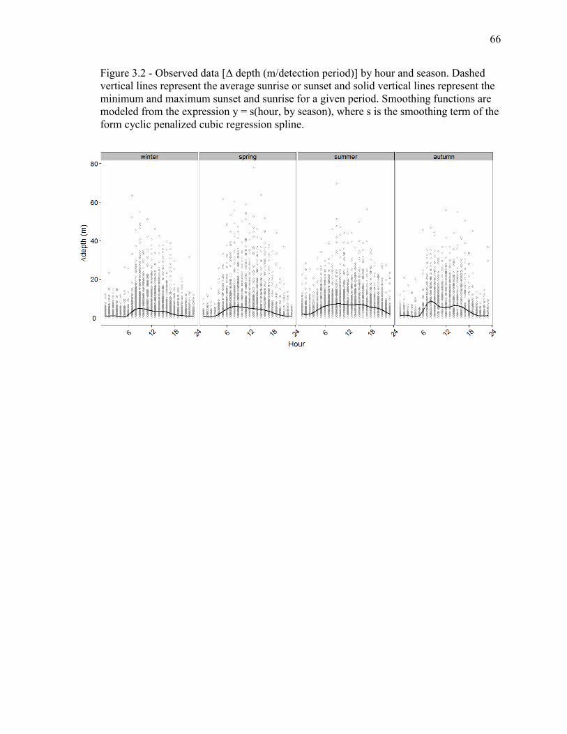
66

Figure 3.2 - Observed data [Δ depth (m/detection period)] by hour and season. Dashed

vertical lines represent the average sunrise or sunset and solid vertical lines represent the

minimum and maximum sunset and sunrise for a given period. Smoothing functions are

modeled from the expression y = s(hour, by season), where s is the smoothing term of the

form cyclic penalized cubic regression spline.

67

Figure 3.3 - Model estimates of bull trout depth (m) by season, diel period (solid line =

night, dotted line = day), and body size (total length (mm)). Shaded regions represent

95% confidence limits for the day (light grey) and night (medium grey). Regions of

confidence limit overlap between day and night periods are emphasized in dark grey.

68

Figure 3.4 - Model estimates of the probability that bull trout change depth by season,

diel period (solid line = night, dotted line = day), and body size (total length (mm)).

Shaded regions represent 95% confidence limits for the day (light grey) and night

(medium grey). Regions of confidence limit overlap between day and night periods are

emphasized in dark grey.

69

Figure 3.5 - Model estimates of change in depth for bull trout by season, diel period

(solid line = night, dotted line = day), and body size (total length (mm)). Shaded regions

represent 95% confidence limits for the day (light grey) and night (medium grey).

Regions of confidence limit overlap between day and night periods are emphasized in

dark grey.

70

Chapter 4: Sex and body size influences on the movement ecology of bull trout

Abstract

Animal movement occurs as a function of many factors including changing

environmental conditions (e.g., seasonality) and the internal state of the focal organism

(e.g., phenotypic traits). Identifying how these factors interact can reveal behavioral

patterns that would otherwise go undiscovered, especially for cryptic free-ranging

animals such as fish. From 2010 to 2012, I used acoustic biotelemetry to examine spatial

distribution, home range size, and total monthly displacement of 187 tagged adfluvial

adult bull trout in relation to several putative factors (year, season, month, body size, sex,

and interactions) in Kinbasket Reservoir. Given the wide range of body sizes, large

number of males and females, and two-year monitoring period, I aimed to reveal how the

movement of tagged fish was related to body size, sex, time of year, and possible two-

way interactions among these variables. Mixed models indicated home range size was

best predicted by body size and season; total monthly displacement was predicted by

month and a two-way interaction between sex and body size. Generally, bull trout

aggregated in a centralized location during winter when individuals occupied relatively

small home ranges (< 25 km2) and had small total monthly displacements. Conversely,

the fall was characterized by a broad distribution of individuals, relatively large home

ranges (> 35 km2), and large total monthly displacements. Bull trout were found to rarely

use the southern portion of the reservoir and the relatively aggregated distribution near

the hydro dam during winter further explains why bull trout entrainment risk is highest

during that period. Large females (~800 mm total length) had a total monthly

71

displacement of up to five times greater than females half their length whereas

movements between large and small males were not significantly different. Sex- and

body-size related differences in activity are attributed to greater reproductive energy

demands and resultant higher activity budgets of large females. This study illustrates

size- and sex related differences in activity outside of the reproductive season and offers

insights for the conservation of bull trout, which are imperiled throughout their range.

72

Introduction

Animal movement is defined as a change in the spatial location of an individual in

time (Nathan et al. 2008). Baseline movement data are a necessary component of wildlife

management (Caro 2007) and animal movement is increasingly investigated in the

ecological and behavioral science literature (Holyoak et al. 2008). While simply

following the movement paths of an animal can illustrate important ecological

information, analyzing the contribution of additional covariates, such as body size and

sex, can help elucidate otherwise overlooked patterns in behavior, such as movement in

the reproductive and non-reproductive periods (Barnett et al. 2011), sex- and size-based

habitat selection (Sims 2005; Laidre et al. 2013), and the consequences of intra- and

interspecific competition (Essington et al. 2000). Furthermore, internal-state factor

interactions are analogous to internal-state dynamics; a rarely discussed aspect of the

movement ecology framework (Nathan et al. 2008). Investigating behavioral

modifications in relation to phenotypic traits, internal-state factor interactions, and their

interactions with environment factors can be highly informative (e.g., Fryxell et al. 2008;

Delgado et al. 2010).

In freshwater and marine fishes, a number of examples exist where movement

patterns can be explained according to phenotype and environmental conditions (Hanson

et al. 2008; Wearmouth and Sims 2008). In Trinidadian guppies (Poecilia reticulata),

experiments have illustrated that predation risk largely drives sexual segregation between

habitats with differing degrees of predation pressure and harassment by the opposite sex

(Croft et al. 2004, 2006). In broadnose seven-gill sharks (Notorynchus cepedianus),

73

males and females exhibit substantial differences in the seasonal timing of migration and

total distance travelled (Barnett et al. 2011). During diel vertical migration, body-size can

have a considerable influence on the timing and range of movement in both prey and

predator fishes (Busch and Mehner 2012). In addition, phenotypic traits are increasingly

recognized as important factors to consider for conservation (e.g., Wearmouth and Sims

2008). However, simply investigating how movement differs among body sizes or

between sexes is challenging, particularly when studying free-ranging animals with large

home ranges.

Biotelemetry and biologging are effective methods to overcome the challenges of

studying free-ranging animals and make inferences about populations (Cooke et al. 2004;

Rutz and Hays 2009; Cagnacci et al. 2010; Hebblewhite and Haydon 2010). Often, high

equipment costs restrict biotelemetry studies to small sample sizes across a small size

range of individuals (to reduce possible unexplained variation associated with body size

on the response) while sex is indeterminable (e.g., species lack secondary sexual

characteristics) or simply ignored as a factor (Hanson et al. 2008). However, with a large

enough sample size and the ability to determine the sex of individuals, biotelemetry can

be used to estimate the influence of phenotypic traits on movement and behavior in wild

populations of fish (Eckert et al. 2008; Wearmouth and Sims 2008).

Here I use biotelemetry to investigate correlative factors of adfluvial bull trout

spatial ecology across multiple seasons in Kinbasket Reservoir. My central hypothesis

was that biotic factors are important determinants of seasonal home range size and

74

movement. I posited that patterns emerging from the influence of phenotypic traits would

provide insights into the movement ecology of free-ranging fishes, information on the

spatial ecology of adfluvial bull trout, and specific information relevant to bull trout in

Kinbasket Reservoir where the population is at risk of entrainment (Martins et al. 2013,

2014). For this study I tagged a wide size range (~350-880 mm total length, Figure 1.2)

of individuals with acoustic biotelemetry transmitters and collected data from these

animals after they travelled among an array of 42 biotelemetry receivers from 2010 to

2012. Mixed modelling and model selection were used to test the hypothesis about home

range size and horizontal movement (measured as total monthly displacement) in relation

to sex, body size, and time of year (season or month). Given that large bodied individuals

possess the capacity to swim at the highest speeds (Brett 1965; Ware 1987; Lightfoot and

Jones 1996), body size was predicted to be positively correlated with both home range

size and total monthly displacement. Given the species’ sensitivity to water temperature

(Selong et al. 2001), bull trout were predicted to have the smallest home ranges during

the warmest and coldest periods of the year, i.e., summer and winter. Reproductive

migrations and their preference for cool water were expected to result in large home

ranges and greater total monthly displacement in the fall months (Barnett and Paige

2013). Given that egg development is energetically costly compared with the cost of

producing sperm and a larger body size requires more energy intake (Gowan and Fausch

1996, Wootton 1998), I predicted large females would possess the largest home range

sizes and perform the greatest horizontal movement over the study period.

75

Methods

The study was conducted in Kinbasket Reservoir which is described in Chapter 1

(Figure 1.4). As described in Chapter 2, data were collected using a 42 omni-directional

VR2W receiver array that was originally deployed in the spring of 2010. Receivers were

retrieved, downloaded, and redeployed in the spring of 2011. Receivers were retrieved

again in the spring of 2012 and removed from the reservoir. Bull trout tagging procedures

are described in Chapter 2. To reiterate from the methods section in Chapter 2, no

receivers were lost in year one whereas in year two, five of the 42 receivers were lost.

Data management and filtering

Data were treated in the same way as in Chapter 2, where false detections and

incomplete tag-to-receiver transmissions were removed prior to analysis. Again, the

minimum number of receiver detections per individual bull trout was set at two per

receiver per 24 hour period. In addition, detections used were those recorded after the

final receiver was deployed in May, 2010. A final data filter was applied to eliminate

estimates from fish that were detected few times during a season (arbitrarily set to < 5

detections/season). Data filtering and exploration were conducted using Microsoft Access

and the R statistical environment (R Development Core Team 2012).

76

Analyses

Seasonal spatial distribution

Seasonal spatial distribution was quantified by assessing the percentage of tagged

bull trout that visited each receiver across Kinbasket Reservoir per season. Percentages

were used to account for an uneven total number of individuals detected per season.

Because receivers were irregularly spaced, the estimates were imported into ArcGIS 10.1

(Environmental Systems Research Institute, Redlands, CA), interpolated by ordinary

kriging, and clipped to a GIS layer of Kinbasket Reservoir. Similarities in the resultant

distribution maps were assessed using the fuzzy Kappa statistic (Hagen-Zanker et al.

2006; Hagen 2003). Fuzzy Kappa compares the similarity of overlaid map cells and their

neighbours where values range between zero (distinct) and one (identical). Average map

similarity was expected to be moderate to high (0.6-0.8; Landis and Koch 1977) between

same seasons during the two year study period. Statistics were generated using the Map

Comparison Kit software v3.2.3 (http://www.riks.nl/mck/index.php; Maastricht, The

Netherlands).

Home range size

For the analysis of home range size, data were examined at the seasonal level

where seasons included: spring (April-June), summer (July-September), fall (October-

December) and winter (January-March). Seasonal classifications roughly correspond to

http://www.riks.nl/mck/index.php

77

biologically meaningful periods for adfluvial bull trout, e.g., the fall is associated with

both reproductive migrations and spawning in lake tributaries (Nitychoruk et al. 2013).

The year variable was defined based on monitoring year (i.e., first monitoring year: May

2010 to April 2011; second monitoring year: May 2011 to April 2012). This classification

ensured that each year contained four seasons which facilitated analyses with factor

interactions (e.g., season x year). Individual bull trout home range size was calculated as

the 90% minimum convex polygons (MCP) from the R package “adehabitatHR”

(Calenge 2006). A minimum number of detections at multiple receivers are required to

calculate MCPs for an individual, thus a biologically meaningful broad-temporal

classification (i.e., season) ensured that a variety of individuals (i.e., wide range of sizes)

would be available for statistical analysis. Although other methods could be used (e.g.,

kernel Brownian bridges, Calenge 2006), MCPs are a simple and commonly used method

for estimating animal home range from acoustic telemetry data (IUNC 1994; Marshell et

al. 2011). In the current study, home range size was calculated as the maximum MCP (%)

that provided estimates for the greatest number of individuals (in this case 90% MCPs).

MCP home range size estimates were exported to ArcGIS 10.1, clipped to a Geographic

Information Systems (GIS) layer of the reservoir, and recalculated in km2. Home range

size was calculated for each individual by season and year.

Total monthly displacement

Distances between receivers were calculated in ArcGIS 10.1 and used to estimate

horizontal movement or, more accurately, the detected (i.e., minimum) total displacement

for each bull trout by month. Estimates based on this method are dependent on the total

78

number of detections. Since estimates almost certainly underestimate distances as time

scale is increased and do not account for tortuous movements between receivers

(Yamanaka and Richards 1993; Rowcliffe et al. 2012), monthly estimates were generated

to reduce the step size (Nathan et al. 2008) and examine total displacement at a scale

finer than season and year. Total monthly displacement was calculated using the R

package “V-Track” which is designed for calculating animal movement from

biotelemetry data (Campbell et al. 2012). To define residency at a receiver, the minimum

number of detections was set at two. Receiver residency for a bull trout was assumed to

be terminated when approximately 30 minutes elapsed between detections at the same

receiver or when the individual was recorded at a different receiver. The sum of the

detected monthly displacement by each bull trout was calculated for each month

(excluding April, 2010) for two years (n = 23).

Statistical modelling procedures

Bull trout home range size and total monthly displacement were analysed using a

GLMM and a GAMM, respectively. For the analysis of home range size, the model

selection procedure began with the full model that included year, season, and sex as

categorical factors, body size [total length (TL) in mm] as the continuous covariate, and

all two-way interactions. For the analysis of total monthly displacement, the model

selection procedure began with a full model that included month as a cyclic smoothing

function (Wood 2006, 2011) and sex, body size, and the sex x body size interaction. Both

models included fish ID as a random factor. Data exploration was performed using

79

standard tools including Cleveland dot plots (to identify outliers) and box and whisker

plots (to identify relationships between continuous and categorical variables) (Zuur et al.

2009). Home range size was log10 transformed to obtain normality. In addition, models

included a variance structure to incorporate heterogeneity in the categorical predictors

(Zuur et al. 2009). Models were fitted to the data using the R packages “nlme” (Pinheiro

et al. 2013) and “mgcv” (Wood 2006, 2011). To determine the most parsimonious model

for home range size, backwards model selection was performed using log-likelihood ratio

tests at α = 0.05. The final models were validated by examining autocorrelation plots and

by plotting the residuals against all variables, including those not retained in the final

model (Zuur et al. 2009). The R package “multcomp” was used to examine all pair-wise

comparisons between the considered categorical factors for home range size (Hothorn et

al. 2008).

Results

Data were logged on the telemetry receivers from May 2010 to May 2012,

yielding approximately 3.5 million bull trout detections. Body size ranged from 358 mm

TL to 881 mm TL with more males detected across all seasons and years (Table 4.1).

More than 20 individuals of each sex were available for analysis within any given season

over the two years (Table 4.1).

Seasonal spatial distribution

80

Between the two years, the fuzzy Kappa analyses showed that seasonal-spatial

distribution was moderately to highly similar (spring Yr1&Yr2 = 0.741; summer Yr1&Yr2 =

0.744; fall Yr1&Yr2 = 0.754; winter Yr1&Yr2 = 0.58). Qualitatively, spatial distribution in year

one varied by season with the greatest proportion of individuals detected in a relatively

small area at the confluence of the Canoe and Columbia reaches during winter and spring

(up to 84 tagged individuals in a 45 km2

area) and winter (up to 39 individuals in a 68

km2 area, Figure 4.1). In the summer, the greatest number of individuals (up to 44) was

detected in small areas near several named creeks in the Canoe Reach (Figure 4.1 ii).

Although the Columbia Reach represented a large portion of the reservoir surface area

during summer (~110 km2 or 26%), relatively few individuals (up to 16) were detected

here. During the fall, relatively large proportions (21-60%) of bull trout were detected

over a long stretch of the reservoir (~75 km) from the Canoe Reach south to the

Kinbasket River in the Columbia Reach (Figure 4.1 iii)). Despite tagging bull trout south

of the Bush Arm, the southern end of the Columbia Reach (Sullivan River south to the

Bush Arm) remained one of the least visited areas for bull trout across all seasons (Figure

4.1).

Home range size

Backwards-model selection indicated that season x year (L-ratio = 11.6, df = 7, P

= 0.11) and sex x body size (L-ratio = 1.44, df = 1, P = 0.23) did not significantly predict

adfluvial bull trout 90% MCP home range size (km2). The most parsimonious model of

bull trout home range size contained season and body size with no interactions (Table

4.2). Home range size was similar between winter and summer (z = 0.1, P = 0.99) and

81

spring and fall (z = 2.5, P > 0.05) whereas all other seasonal home range size

comparisons were significantly different (in all cases, P < 0.01). Large bull trout (765

mm TL) occupied the largest home range during the spring [mean: 46.0 km2, 34.4, 61.6,

95% confidence interval], whereas the smallest home ranges were estimated for small

bull trout (470 mm TL) during the summer and winter [meansummer: 13.6 km2, 10.0, 18.4,

95% confidence interval, and meanwinter: 13.4 km2, 9.6, 18.6, 95% confidence interval,

Figure 4.2].

Total monthly displacement

According to backwards model selection, the full model was the best model to

explain total monthly displacement (km) in bull trout (Table 4.2). The smoothing term,

coded as a numerical variable, was significant and showed patterns in total monthly

displacement across two years for male and female bull trout (♂: t = 8.66.8, P < 0.0001;

♀: t = 8.312.3, P < 0.0001, R2 = 8.7%, Figure 4.3). On average, large fish (800 mm TL)

moved greater distances than small fish (400 mm TL) in a given month; however the

difference was significant only among females (Figure 4.4). For females during a given

month, large fish were predicted to move as much as five times further than smaller

conspecifics (Figure 4.4). The predicted trend in movement indicated that total

displacement was greatest in the spring (May through June) and fall (October through

December) while the least total displacement occurred during the winter months (January

through March). Although patterns remained consistent across seasons for the two years,

the amplitude of these patterns across years was higher in the fall months for year one

than in year two, both for males and females (Figure 4.4). The average differences in

82

predicted monthly movement between years for the months of August through December

were 14.9 km ± 7.3 SD for small males, 23.1 km ± 5.7 SD for small females, 15.0 km ±

7.3 SD for large males, and 23.1 km ± 5.7 SD for large females.

Discussion

Biotic factors, namely sex and body size, were significant predictors of adfluvial

bull trout movement, however these factors did not explain home range size (Table 4.2).

In addition, there was a sex x body size interaction to explain horizontal movement over

time (Figure 4.4). This interaction is an overt example of internal-state dynamics from the

movement ecology framework (Nathan et al. 2008). The majority of work on organismal

movement simply documents movement or describes how it was influenced by the

environment (Holyoak et al. 2008). However, movement derives from a number of co-

occurring causes and mechanisms (Bennetts and Kitchens 2000; Long et al. 2008;

Mehner 2012), which may be further complicated by relationships within, for example,

the internal state of an organism. As illustrated here in adfluvial bull trout and in a

number of other species (e.g., bluefin tuna, Thunnus maccoyii; Bestley et al. 2010, elk,

Cervus elaphus, Fryxell et al. 2008, eagle owls, Bubo bubo, Delgado et al. 2010),

putative factors corresponding to the internal state and external factors predict where,

when and how often organisms move (Nathan et al. 2008).

Periodic changes in the abiotic and biotic environment (e.g., temperature) can

have a predictable set of outcomes for the behavior of ectotherms (e.g., Sims et al. 2001;

Morley et al. 2007; Kearney et al. 2009). Given that temperature is the master controlling

83

factor of fish physiology and behavior (Brett 1971), yearly, seasonal, and monthly

differences in temperature can have a significant influence on activity (Arendt et al. 2001;

Bestley et al. 2010). Behavior in free-ranging fish is commonly explained by seasonally

fluctuating environmental factors such as periodic changes in temperature (Sims et al.

2004), light (Schruell and Schindler 2003), and dissolved oxygen (Moreley et al. 2007).

In addition, it is increasingly apparent that fish movement can be context- (Dingemanse

et al. 2010; Sih et al. 2012) or personality-dependent. For example, reef populations of

golden-lined rabbit fish (Siganus lineatus) exhibit a different diel foraging strategy than a

population from a boulder-shoreline site (Fox and Bellwood 2011). In Kinbasket

Reservoir, individually tagged burbot were found to exhibit seasonally-dependent

movement that was repeatable for individuals independent of body size, e.g., individuals

that moved long distances in summer also did so during winter (Harrison et al. In Press).

Given that forage fish are generally less abundant in the spring compared to the

previous fall (Sogard 1997; Suski and Ridgeway 2009), the wide distribution, large home

range sizes, and relatively high activity of individual bull trout may be attributed to the

distribution of their prey (Figures 4.3 and 4.4). Adfluvial bull trout perform DVM and

exhibit their deepest swimming depths during summer, probably in response to warmer

surface temperatures (Chapter 3). Light attenuates quickly with depth and if large

horizontal movements do not result in increased encounters with prey, bull trout may

continue performing DVM to hunt during summer (i.e., when the reservoir develops a

thermal gradient, Bray 2012; Chapters 2 and 3) while only maintaining small home

ranges and embarking on limited horizontal movements. It is reasonable to predict that

84

the limited movement observed in summer is, in part, explained by bioenergetic

requirements of bull trout and the distribution of kokanee salmon prey which perform

diel vertical migration (Bevelhimer and Adams 1993; Vogel and Beauchamp 1999). In

fall, the high percentage of individuals detected across much of the reservoir, the large

total monthly displacement, and large home ranges (Figure 4.1, iii) are most easily

explained as a response to cooling water temperatures (i.e., bioenergetics efficiency), the

reproductive migratory behavior of prey (feeding opportunity hypothesis, Olmsted et al.

2001), and the fall reproductive migratory behavior of bull trout which is an adaptation of

charr and based on environmental cues (e.g., temperature and solar radiation, Dingle

1996). Home range size and displacement were minimal in winter, likely to conserve

energy while continuing to vertically migrate and feed on kokanee (Beauchamp and Van

Tassell 2001; Helland et al. 2011; Chapter 3).

Body size is a well-known predictor of home range size in mammals, birds,

reptiles, and for some species of fish (Reiss 1988; Minns 1995; Haskell et al. 2002;

Eckert et al. 2008). Large bull trout had the largest home ranges (~ 45.5 km2

during

spring), a pattern that corroborates with the positive relationship found between body size

and total monthly displacement (Figure 4.4). To my knowledge these are the first data to

describe adfluvial bull trout home range size. Unlike for adfluvial bull trout, fluvial

conspecifics have been shown to possess small home ranges with no effect of body size

(Schoby and Keeley 2011). It is likely that the distribution and abundance of food

resources in some bull trout rivers may not necessitate larger home ranges for large

individuals (i.e., optimal foraging theory, Werner and Hall 1974; Pyke 1984). Although

85

kokanee salmon are abundant in Kinbasket Reservoir, the larger size classes are rare and

dispersed (Sebastian and Johner 2011). However, contrary to my prediction, sex was not

a significant predictor of home range size (Table 4.2). Home range size is not always

different between the sexes (Norman and Jones 1984), and the relationships among sex,

body size, home range and movement tend not to be universal among fishes (Croft et al.

2003). The simplest interpretation of this relationship is that compared to male bull trout,

the average female moves more frequently within their home range. However, this

relationship is further complicated by the sex x body size interaction predicted in

horizontal movement.

Sexual-size dimorphism has consequences related to growth, activity, and

behavior both during and outside of the breeding season (e.g., Henderson et al. 2003;

Rennie et al. 2008; Nitychoruk et al. 2013). For example, Nitychoruk et al. (2013) found

seasonal and sex-related differences in body condition where the summer body condition

of adfluvial bull trout was relatively poor compared to that of the spring but that females

during the fall possessed better body condition than males during the same season. In the

current study, the magnitude of the total horizontal displacement was explained by a body

size x sex interaction in which only large females moved significantly farther than small

individuals of the same sex (Table 4.3; Figure 4.4). It should be noted, however, that only

a small amount of the variation was explained by the smoother for month (R2 = 8.7%).

Bahr and Shrimpton (2004) also reported a large variance in monthly movement for bull

trout across tributary systems in the Morice River watershed system, BC. Nevertheless,

assuming the relationship is biologically significant despite a low R2, one possible

86

explanation for the body size x sex interaction is an extension of the activity budget

hypothesis which has mainly been used to predict sexual segregation in sexually size-

dimorphic ungulates and marine animals including fish (Ruckstuhl 2007; Wearmouth and

Sims 2008). The hypothesis suggests that sexually size-dimorphic species exhibit sex-

based differences in energetic requirements, digestive efficiencies and possibly also

movement rates which result in the formation of single-sex groups (Rennie et al. 2008;

Wearmouth and Sims 2008). However, sex-based differences in activity can also exist

independent of body size. For example, similarly sized male and female small-spotted

catshark (Scyliorhinus canicula) have been shown to differ in activity, where females

exhibit more intense foraging behavior compared with males (Kimber et al. 2009). It is

reasonable to suggest that compared to similarly-sized males, the relatively high activity

in large-sized females is related to more intense foraging behaviour to accumulate the

greater energy required for female reproductive tissue development (Hendry and Berg

1999; Kimber et al. 2009; Yong and Grober 2014).

Body size is positively correlated with foraging time when large prey are rare and

given that gamete production is more costly for females than for males, females should

be foraging-time maximizers whereas male fish should theoretically minimize foraging

time (Schoener 1969; Hoffman 1983). In addition, the risk of predation for the largest

fish is probably minimal, thus increased activity would not result in a high cost to

survival (Werner and Anhold 1993). Although large males may prefer larger prey than

smaller individuals of the same sex, the difference in horizontal movement here is

marginal (Figure 4.4). To meet the energetic requirements associated with female

87

reproduction, large mature females may spend more time foraging while searching for

rare but optimally sized prey. While increased movement may be energetically costly and

risky (Werner and Anhold 1993), the benefits could include increased encounters with

optimally-sized prey (Werner and Hall 1974), better body condition (Nitychoruk et al.

2013), and increased energy for reproductive tissue development in females. Again

however, the adjusted R2 for the smoother is low, although not necessarily for biological

studies (Møller and Jennions 2002), and my predictions remain to be tested together in

the field.

Despite their conservation status, relatively little is known about bull trout spatial

ecology in reservoir systems where this species is widely found. Overall, the data

collected here in Kinbasket Reservoir were highly informative both as a means to

investigate hypotheses related to movement in free-ranging organisms and provide

information for the conservation of bull trout, which are imperiled throughout most of

their range. For example, winter activity has been shown to occur in other lacustrine bull

trout populations (Salow and Hostettler 2004; Dare 2006) and the spatial distribution in

Kinbasket Reservoir illustrates why entrainment risk is highest during this season

(Martins et al. 2013, 2014). Despite tagging 15% of the sample from tributaries at

southern part of the system, bull trout rarely used this location outside of the reproductive

period (Figure 4.1). The results from this research chapter could be useful for fisheries

managers who are considering mitigation or compensatory activities (e.g., spawning site

restoration) to offset entrainment-related losses (Martins et al. 2013).

88

In summary, by pairing biotelemetry data with temporal changes in the

environment and phenotypic traits, I found patterns in behavior that would otherwise go

unidentified in these free-ranging animals, e.g., internal-state dynamics (Nathan et al.

2008). I have suggested mechanisms that underlie the behaviors, however further

investigation is required. Given the sophisticated technology, statistical tools, and

software available to study the behavior of wild and cryptic animals such as fish, there

are ample opportunities to conduct similar research that could reveal information that is

pertinent to behavioral ecology, movement ecology, and species’ conservation.

89

Tables

Table 4.1- Sample size by year, season, sex, and body size for the home range size and

horizontal movement analyses of adfluvial bull trout in Kinbasket Reservoir.

Home range Horizontal movement

Count Range (TL mm) Count Range (TL mm)

Factor f m f m f m f m

2010-2011

spring 43 66 515-786 434-881 45 71 393-765 434-881

summer 35 48 393-741 440-881 62 84 358-786 434-881

fall 56 73 358-786 434-881 47 71 515-786 434-881

winter 45 65 393-786 362-881 53 75 393-786 362-881

2011-2012

spring 47 74 451-786 434-881 34 58 445-741 434-881

summer 21 51 467-741 434-881 36 60 465-786 434-881

fall 29 50 515-786 434-881 52 82 445-786 362-881

winter 29 32 515-786 434-881 35 46 501-786 434-881

90

Table 4.2- Summary of the importance of individual terms, including a variance structure (var) for the GLMM on home range

size. Residual standard deviation for the random effect in both the GLMM and GAMM were 0.566 and 52.68 respectively.

Model model term t-value L-ratio P-value

GLMM-

Home

range size Intercept 4.87 <.0001

Season 50.5 <.0001

TL 4.36 0.034

(var) 44.5 <.0001

GAMM-

Movement Intercept 1.64 0.139

TL 22.2 <.0001

Sex 10.2 0.007

Sex x TL 7.05 0.008

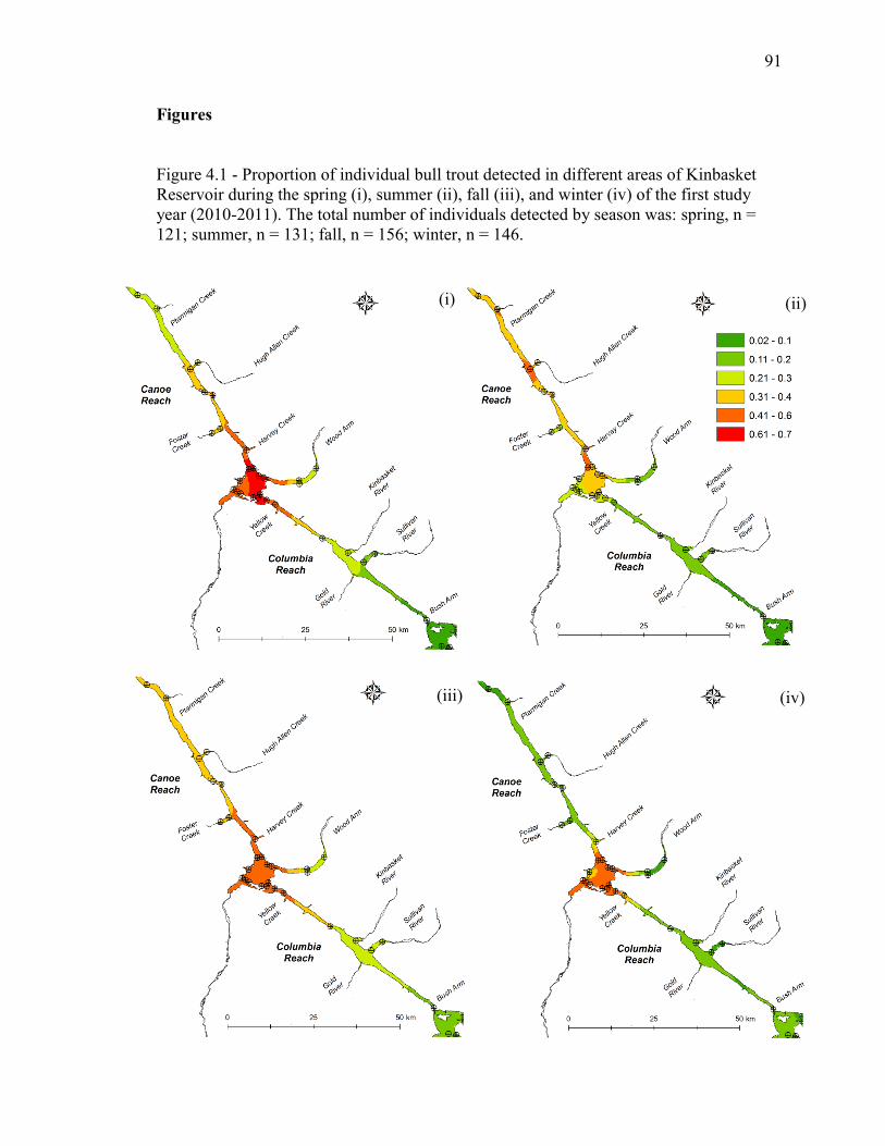
91

Figures

Figure 4.1 - Proportion of individual bull trout detected in different areas of Kinbasket

Reservoir during the spring (i), summer (ii), fall (iii), and winter (iv) of the first study

year (2010-2011). The total number of individuals detected by season was: spring, n =

121; summer, n = 131; fall, n = 156; winter, n = 146.

(iii) (iv)

(i) (ii)

92

Figure 4.2 - GLMM predictions of adfluvial bull trout home range size (mean km2 ± 95% confidence limits) by body

size (total length, mm) and season in Kinbasket Reservoir, British Columbia.

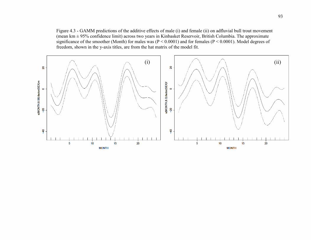
93

Figure 4.3 - GAMM predictions of the additive effects of male (i) and female (ii) on adfluvial bull trout movement

(mean km ± 95% confidence limit) across two years in Kinbasket Reservoir, British Columbia. The approximate

significance of the smoother (Month) for males was (P < 0.0001) and for females (P < 0.0001). Model degrees of

freedom, shown in the y-axis titles, are from the hat matrix of the model fit.

(i) (ii)

94

Figure 4.4 - Predicted large (800 mm TL) female (dashed line round marker), small (400 mm TL) female (dashed line

square marker), large male (solid line triangle marker), and small male (solid line diamond marker) adfluvial bull trout

horizontal movement (mean km ± 1 SE) across two years in Kinbasket Reservoir, British Columbia. For clarity,

estimates are shown with standard errors.

0

20

40

60

80

100

120

140M

ean

to

tal d

isp

lace

men

t

(km

± 1

SE)

95

Chapter 5: General Discussion

Adfluvial bull trout selected their thermal habitat as environmental temperature

availability changed, and phenotypic traits and environmental factors interacted to

explain the size (e.g., home range), shape (e.g., horizontal movement), and direction (e.g.,

diel vertical migration) of adfluvial bull trout movement in Kinbasket Reservoir. To

synthesize all of these findings, I will use the movement ecology framework and the

current literature on bull trout behaviour and movement. I will also discuss biotelemetry,

mixed-modelling, the implications for bull trout conservation, and several research

opportunities.

There are five basic questions in the movement ecology framework: (i) why

move? (ii) how to move? (iii) where and when to move? and (iv) what are the ecological

and evolutionary consequences of movement (Figure 1.1)? The acoustic telemetry system

and modern statistical techniques (discussed later) were appropriate methods for

addressing these questions and by collecting data on phenotypic traits and environmental

data, I could directly examine how the internal state, motion capacity, and navigation

capacity interacted with external factors to produce and influence movement. For

example, putative internal and external factors made it possible to hypothesize about

proximate drivers and ultimate causes responsible for diel vertical migration (Chapter 3).

In the following subsection I will discuss each component of the movement ecology

framework as it relates to the finding of my three research chapters.

96

The internal state

The internal state addresses the question, “why move?” and there are both

proximate and ultimate payoffs for choosing to move (Nathan et al. 2008). Thermal

resource selection, diel vertical migration, and homerange size were each affected by

variables that represented the internal state of tagged bull trout (i.e., phenotypic traits,

Delgado et al. 2010). Larger individuals were predicted to experience slightly but not

significantly warmer temperatures than smaller conspecifics (coefficients not shown but

see Table 2.1 and 2.2), swim at the shallowest depths, and possess larger home ranges. In

addition, larger females were predicted to move greater distances than smaller females.

According to these results, the choice to move is related to environmental temperature

and phenotypic traits. Indeed, the choice whether to move is possibly also related to the

distribution of predators and prey which individuals may choose to avoid or pursue based

on their internal state (e.g., body size). Additionally, larger individuals are at a decreased

risk of predation due to gape limitations of piscivorous predators (Wootton 1998),

although as discussed in Chapter 2, swimming at a particular depth does not directly

show that predation risk/feeding opportunities are the mechanisms that drive such

behaviour. Such a study would require a different approach (discussed later in the mixed-

modelling and future research opportunities sections). The interaction between body size

and sex illustrates internal-state dynamics across changing environmental conditions,

e.g., seasons (Nathan et al. 2008, Figure 1.1). This aspect of the movement ecology

framework is rarely discussed in the movement ecology literature. As with diel vertical

migration hypotheses, no single hypothesis/variable is sufficient to predict behaviour.

Instead, movement paths are generated from a dynamic interplay of variables that include

97

external factors, the internal state, the capacity to move, and the navigation capacity

(Nathan et al. 2008; Holyoak et al. 2008).

Motion capacity

The question of “how to move?” is largely related to the internal state and external

factors that drive how an organism moves. For instance, movement rate is influenced by

the internal state (body size) and external factors (competitors, in Chapter 3). In Chapter

4, home range size could be predicted by the internal state, navigation capacity, and the

external factors that underlie seasonal change. Horizontal distance moved was also shown

to differ seasonally and by the internal state and motion capacity, seasonal change

(external environment and navigation capacity), and phenotypic traits. Describing how an

organism moves (e.g., rate, magnitude, dispersal) in relation to, for example, external

factors is the most commonly made link in the movement ecology literature (Holyoak et

al. 2008). Not surprisingly, the link between motion capacity (e.g., home range size) and

the environment was common among my work in Kinbasket and among other research

on adfluvial bull trout movement (e.g., Brenkman et al. 2001; Wissmar and Craig 2004;

Watry and Scarneccia 2008; DuPont et al. 2011). For example, depending on sex and

body size, bull trout were estimated to make monthly movement ranging from

approximately 5-120 km/month (Figure 4.4). While their methods to calculate monthly

movement were different, Bahr and Shrimpton (2004) estimated a similar though slightly

smaller range of monthly distances moved (i.e., ~ 0-75 km/month) by bull trout in the

98

Morice River watershed in BC. Again, these estimates are completely dependent on the

step size (Rowcliffe et al. 2012) and I would suggest bull trout likely move far greater

distances, perhaps an order of magnitude, than estimated from the Kinbasket system.

Speaking strictly in terms of the biomechanical aspect of movement (e.g.,

Dickinson et al. 2000), bull trout use body caudal fin propulsion and a sub-carangiform

swimming mode (Sfakiotakis et al. 1999). Currently, literature on wild bull trout

swimming performance is limited to a small number of lab studies (Mesa et al. 2004;

Mesa et al. 2008). Additional data from the V-Track (Campbell et al. 2012) R package

used in Chapter 3 estimated that bull trout rate of movement between telemetry receivers

ranged between approximately 0.0001 m/s and 1.46 m/s. Given that these estimates are

based only on Euclidean distances and the time taken by a bull trout to appear at one

receiver from another, I chose not to include or model these data. Although some of these

values may be accurate approximations of wild bull trout swimming behaviour, whether

swimming performance was sustained, prolonged, or burst (Beamish 1978; Plaut 2001),

there is no way of knowing where and when fish made linear movements between

receivers. Here, values at the lower end suggest that bull trout took a curvilinear path

before reaching another receiver whereas values at the upper end of the V-Track

estimates were similar to slow sprints in this species (Mesa et al. 2008). In 2010, while

undertaking a side project on injury and immediate mortality of bull trout captured in the

spring troll fishery on Kinbasket Reservoir, fish regularly pursued minnow-plug lures at

speeds in excess of 1.5 ms-1

(Gutowsky et al. 2011). Interestingly though, “wild” bull

trout in the lab will not perform sprints in water temperatures of 6°C (Mesa et al. 2004)

99

yet wild bull trout in Kinbasket were captured by trolling at speed considered “sprints”

and at water temperatures of 2°C (Gutowsky et al. 2011). The field-based troll fishery

capture data and lab-based bull trout swimming performance data demonstrate that more

research is required on bull trout motion capacity.

In addition to locomotion through body-muscle contraction, bull trout may also

use their swim bladder to change swimming depth. In fishes, the swim bladder is air-

filled sac located in the coelomic cavity below the vertebral column (Holbrook and

Perera 2011). Bull trout have swim bladders that are connected to the mouth by the

pneumatic duct (i.e., physostomus). This allows for rapid inflation and deflation of the

organ. Among its functions, the swimbladder can be used to regulate buoyancy. Holbrook

and Perera (2011) suggested that physostomus fish use hydrostatic pressure to determine

their depth and, by regulating their swimbladder, remain neutrally buoyant. While little is

known about the energetic costs associated with hydrostatic pressure change (Speers-

Roesch et al. 2004) or the exact proximate function of swimbladder regulation for DVM

(Mehner 2012; Solberg and Kaartvedt 2014), it remains feasible that both swimming and

swimbladder regulation are operational modes of bull trout motion capacity.

Navigation capacity

Navigation capacity addresses the questions of where and when to move. The

choice of when and where to move is based on the goal (e.g., to attain food, mate, hide)

100

and an environmental assessment by the sensory systems (Bleckmann 1986; Dittman and

Quinn 1996; Hara and Zielinski 2006). In other words, navigation capacity largely

involves input from the internal state and external factors (Figure 1.1). Although sensory

mechanisms were not exclusively tested in adfluvial bull trout, the questions of where

and when to move were integrated and addressed in each research chapter. For example,

decreased availability of optimal temperatures for metabolism and growth is likely

responsible for changing thermal resource selection over time (Figure 2.4). Location in

the water column was related to diel period, season, and body size. Here, bull trout

movement largely relates to light levels that change over a 24 hour period. Location in

the reservoir (i.e., distribution) also appeared to be related to season and was repeatable

across years (Figure 4.1).

Throughout my research chapters, I discussed the likely underlying goals (i.e., of

bull trout) that led to the patterns observed in the telemetry data. For instance, bull trout

use sensory information from the environment to move to a depth where food is most

likely to be obtained (Chapter 3). DVM likely occurs in part because bull trout are

visually detecting prey (Henderson and Northcote 1985; Vogel and Beauchamp 1999;

Mazur and Beauchamp 2003; Muhlfeld et al. 2003). Additionally, individuals made

decisions based on their body size, with the largest individuals inhabiting the shallowest

water with presumably the most available light (Figure 3.3). Although reproductive

migrations were not observed in this research, individuals likely use water temperature,

flow, and chemical cues to commence migration and locate natal spawning grounds

(McPhail and Murray 1979; Fraley and Shepard 1989; Lucas and Baras 2000; Hodgson

101

and Quinn 2002). In winter, individuals congregated at the confluence of the Columbia

and Canoe Rivers. Here, temperature change and ice cover (e.g., changes in light levels)

may have resulted in this behaviour. Again, as indirectly demonstrated in the behaviour

of adfluvial bull trout, individuals use sensory input from their environment and input

from their internal state (Figure 1.1).

External factors

External factors represent all aspects of the abiotic and biotic environment.

External factors play a key role in determining the activity and behaviour of all organisms

(Holyoak et al. 2008). Given the apparent importance of temperature to cold-water

stenotherms such as bull trout (e.g., Jones et al. 2013), I investigated the relationship

between the amount of thermal habitat available and the temperature these animals

selected. Adfluvial bull trout did exhibit thermal resource selection as the external

temperature changed (Figure 2.4). In Chapter 3, I found that bull trout vertical movement

was strongly related to diel period. As with other salmonids (Levy 1990, 1991; Jensen et

al. 2006), activity was explained by light levels in the external environment. Additionally,

the same environmental variables influence vertical activity in burbot (Harrison et al.

2013). For bull trout, environmental factors (e.g., temperature, landscape features) are

often the primary focus of investigations regarding movement (e.g., Swanberg 1997;

Bahr and Shrimpton 2004; Muhlfeld and Marotz 2005; Howell et al. 2010). Similarly,

external factors were the most commonly investigated variable among our team’s

research on Kinbasket. In the literature on organismal movement, nearly 2/3 of all

102

research examines external factors only on the occurrence or frequency of movement

(Holyoak et al. 2008). As seen here in adfluvial bull trout, external factors, particularly

temperature, are important modifiers of ectotherms behaviour (Bardach and Bjorklund

1957; Brett 1971; Wieser 1973; Zug et al. 2001).

The movement path

As demonstrated in the movement ecology literature (e.g., Fryxell et al. 2008;

Mandel et al. 2008; Owen-Smith et al. 2010), movement paths are dependent on the scale

of study and may be illustrated as steps, phases, and the lifetime track (Nathan et al.

2008). Steps are based on the difference between two points in time given the spatial and

temporal scale of the study. Step length for temperature and depth was limited by the

transmission rate of the telemetry tags (2-6 minutes), thus the resolution was relatively

fine-scale for these studies. On the other hand, the analysis of homerange and horizontal

movement required large step lengths that spanned the distance between receivers. For

each study, movement-related questions were based largely on the step length and the

limitations of the technology.

While some empirical investigations show tracks by individuals (e.g., Bestley et

al. 2010), such movement paths are not always illustrated in studies of animal movement

(Holyoak et al. 2008). Among studies of adfluvial bull trout movement, actual individual

movement paths are not shown. In the Kinbasket system, individual movement paths

were not the focus of any investigation, rather questions more commonly involved

103

motion capacity while movement paths were implied and discussed. Indeed, with 187

individuals tagged in Kinbasket and a potential step length of 2-6 minutes for depth and

temperature detections across one year or more, it is unreasonable to plot and present all

of the individual movement paths. Instead, most of my investigations examined the fish

as collective group-level patterns in behaviour and movement that were associated with

motion capacity, navigation capacity, internal state, and external factors.

A synthesis of the movement ecology of adfluvial bull trout

Here I synthesize the movement ecology of adfluvial bull trout based on

seasonality. Seasonal movement regards questions about when to move while also

representing a period of environmental change, i.e., a change in external factors. Season

is commonly associated with organismal movement, particularly in fish. For instance,

reaction distances for salmonids such as lake trout (Salvelinus namaycush), rainbow trout

(Oncorhynchus mykiss), and cutthroat trout (Oncorhynchus clarki) are dependent on light

levels, the spectral properties of light, and turbidity (Henderson and Northcote 1985;

Vogel and Beauchamp 1999; Wetzel 2001), which are environmental variables that

change seasonally. While seasons span several months and as a predictor of movement

may only explain a portion of the total variation (e.g., vertical movement, Figures 3.2 and

3.5), seasons represent periods of abiotic and biotic change that are among the most

important variables for directing ectotherm behaviour (e.g., Young 1998; Nowak and

Quinn 2002; Deutsch et al. 2008). Although the cut-off points for astronomical season

does not necessarily correspond to all abiotic and biotic changes, astronomical season

104

was assumed to be a reasonable approximation of biologically significant changes in the

environment (Suski and Ridgeway 2009).

Winter

During winter, adfluvial bull trout experienced increasingly cold water up to a

minimum average between 1 and 2°C from January to April (Figure 2.3). These patterns

were evident in both 2010 and 2011. Despite the low temperatures and perhaps low-light

levels due to ice cover (data on ice cover were unavailable), bull trout continued to

exhibit diel-related patterns in movement including DVM and vertical movement

(Figures 3.1 and 3.4). Patterns in DVM and vertical movement remained size-dependent

where larger fish occupied shallower depths and performed greater depth changes.

Estimates of winter homerange size were similar to summer estimates (Figure 4.3) while

winter movement was low, especially for small males (Figure 4.4). However, large fish,

especially females, were estimated to make horizontal movements of at least 80

km/month during the winter (Figure 4.4). Winter activity has also been shown in bull

trout in Arrowrock Reservoir, Idaho (Salow and Hostettler 2004; Dare 2006), a small

alpine lake in the Canadian Rocky Mountains (Whilhelm et al. 1999), and in a study on

bull activity and entrainment in Kinbasket Reservoir (Martins et al. 2014). Most bull trout

in Kinbasket experienced cold winter water temperatures and performed vertical

movement behaviours in an area that spanned the confluence into both the Columbia and

Canoe Rivers (Figure 4.1). Wild adfluvial bull trout do pursue prey in 2°C water

(Gutowsky et al. 2011) and likely actively hunt during winter (Wilhelm et al.1999;

Beauchamp and Van Tessel 2001). This activity, both on a vertical and horizontal plane,

105

partly explains the relatively high likelihood of entrainment during the winter (Martins et

al. 2013).

Spring

Most adfluvial bull trout were sampled by trolling in the spring when these

animals are especially vulnerable to capture but resilient to angling induced stress and

immediate mortality (Gutowsky et al. 2011). Given the magnitude of vertical activity

(Figure 3.5), large home range sizes (Figure 4.2), and large monthly horizontal

movements (Figure 4.4), it appears that adfluvial bull trout are most active during spring.

Although bull trout performed vertical migrations in the spring, depth distribution was

not related to body size at this time (Figure 3.3). While I attribute this anomaly to the lack

of competition during spring, e.g., sympatric adfluvial rainbow trout spawn during spring,

additional research is required. More so than winter, individuals were concentrated in the

main basin of the reservoir (Fraley and Shepard 1989, DuPont 2011, Figure 4.1). The

congregation of bull trout likely results from a combination of factors including relatively

high flow, high nitrate, low conductivity, high water clarity in the confluence compared

with other areas of the reservoir (Bray 2011, 2012). Based on the large home ranges and

extensive horizontal movements in spring, it would appear that individuals patrolled the

confluence area at this time. While sampling during spring, our team witnessed sporadic

kokanee salmon activity near the surface. Kokanee are a preferred food source for bull

trout during spring (Beauchamp and Van Tessel 2001) and I expect that the abiotic

106

characteristics of the confluence are an attractant for numbers of kokanee and bull trout in

this reservoir.

Summer

As expected, adfluvial bull trout experienced the warmest temperatures during

summer. However, the average temperatures experienced were close to the optimal

temperatures for growth and metabolism in juveniles of this species (Figure 2.3). These

results are not consistent with the literature that shows final temperature preference

should be markedly lower in larger fish (Coutant 1977, Elliott and Allonby 2013 and

references therein). Contrary to using free-swimming fish, these studies are lab-based

where individuals are not subject to numerous external factors including access to shelter,

predators, and dispersed prey (Elliot and Allonby 2013). During summer, small bull trout

actually experienced cooler temperatures than larger conspecifics (Chapter 2). This may

indicate that adfluvial bull trout are balancing a trade-off between maximum growth

efficiency and predation risk depending on body size (Jonsson and Jonsson 2011; Mehner

et al. 2013; Chapter 2). As water temperatures began to cool in late-summer to early

autumn, bull trout selected water temperatures that were close to the optimal

temperatures for juvenile growth (Figure 2.4). Selection for such temperatures continued

as the availability of these temperatures declined. In Kinbasket during summer, bull trout

were observed to occupy average depths between to 10 and 20 m (Figure 3.1), suggesting

that diel vertical migration occurred approximately within the window of selected

temperatures and probably light levels. Bull trout made large vertical movements during

the summer and, for a given body size, were predicted to occupy some of the deepest

107

water, presumably to avoid intense summer UV light and surface temperatures that were

above their apparent temperature preference of approximately 12°C to 13°C (Figure 2.3).

Unlike in Lake Billy, Oregon, where adult adfluvial bull trout were only found in the

river during summer (Beauchamp and Van Tessel 2001), a large proportion of tagged

Kinbasket bull trout (70%, 131/187) were found most evenly distributed across the

reservoir where they possessed small home ranges and made small horizontal movements

during approximately the same time frame (Figures 4.1 and 4.4). In Kinbasket, at least

some individuals certainly spent time in the reservoir during summer where they selected

optimal water temperatures and performed DVM within a limited area. In summary, the

summer was the period when bull trout experienced the warmest temperatures, occupied

deep water, and made limited horizontal movements that were dependent on sex and

body size.

Autumn

In autumn, bull trout temperature experience dropped sharply (Figure 2.2) and as

the warmest temperatures became less available (Figure 2.1), thermal resource selection

increased for this temperature category (Figure 2.4). DVM continued to occur in the

autumn when the observed data reflected the most prominent patterns of descent at dawn

and ascent at dusk (Figure 3.1). Home range size and horizontal movement were

maximized during the autumn, presumably because at least some of the tagged

individuals had migrated into tributaries to reach spawning grounds, and because cooling

water temperatures led to increased activity (Figures 4.3). Kokanee salmon also spawn

during fall and it has been suggested that adfluvial bull trout may move into and out of

108

spawning tributaries to feed (Beauchamp and Van Tessel 2001; Barnett and Paige 2013).

The body condition for bull trout in Kinbasket is poor during the late-summer to early

autumn (Nitychoruk et al. 2013) and likely declines further after spawning (Mushens and

Post 1997; Wilhelm et al. 1999). Whereas the summer is a period of relative inactivity for

adfluvial bull trout, movement significantly increases during the autumn (DuPont et al.

2011). This remains true for bull trout in both lakes and rivers (Bahr and Shrimpton

2004). I suspect the increase in activity is likely for reproductive purposes and to build fat

stores for the winter. However, these hypotheses remain to be tested.

Biotelemetry and mixed-modelling for movement ecology

Biotelemetry

For the past 50 years biotelemetry has been a useful means of studying the

movement of free-ranging organisms (Stasko and Pincock 1977; Kephart 1980; Cooke et

al. 2004). For adfluvial bull trout, the characteristics of acoustic biotelemetry, namely its

ability to transmit signals in deep water (Heupel et al. 2006), rendered it the best system

for recording data on free-ranging individuals in Kinbasket Reservoir. Since the internal

application of transmitters required handling individuals, I was able to collect information

on phenotypic traits including body size and sex (e.g., Delgado et al. 2010). Once the

animal was released, the internal clock of the acoustic biotelemetry system made it

possible to align the times of relocations to external factors such the time of day, times

for sunset and sunrise, and astronomical season. Then, given the questions and

hypotheses, I could then pair explanatory variables (e.g., external factors) with a response

109

variable (e.g., a measure of motion capacity) and use mixed-modeling techniques and

model selection as a means to test hypotheses (Anderson et al. 2000).

Mixed-modelling and model selection to analyse movement data from

biotelemetry

By collecting data from multiple individuals and analysing data with mixed-

modelling techniques, I was able to use biotelemetry to make generalized inferences

about adfluvial bull trout (Giuggioli and Bartumeus 2010; Cooke et al. 2004). As

discussed in Chapter 4, biotelemetry data are well suited to mixed-modelling because

they are easily paired (spatially and temporally) with additional data about the

environment and the individual organism. A random intercept for each individual

assumes that observations from an individual are more alike to one another than to those

from another individual. Random effects have a certain mean and variance that can be

included in the model and thus allow for general statements about the group (e.g.,

population).

Once the appropriate fixed and random components have been identified (i.e., a

priori hypothesized biologically significant explanatory variables, Anderson et al. 2000),

telemetry data can be analysed using a model selection procedure. I used multiple

approaches to select the best model to explain adfluvial bull trout movement. For

instance, based on model P-values , backwards model selection, or an information

theoretic approach. The model selection procedure depends on the initial questions and

hypotheses. For example, in Chapter 4 I used backwards model selection to provide the

110

relative contribution of individual terms in the nested models, which was useful for

interpreting the biological importance of the hypothesized covariates of these models

(Zuur et al. 2009). Temperature experience data (Chapter 2) were analyzed using an

information theoretic approach, where all possible models were a priori assumed to

require a smoothing function for day. Models were then built up to a set of candidate

hypotheses (Burnham and Anderson 2002). The information theoretic approach was

useful because I was able to evaluate multiple non-nested models, quantify the relative

support for multiple models simultaneously, and if necessary, derive predictions that

account for model uncertainty using model averaging (Burnham and Anderson 2002;

Zuur et al. 2009).

While statistically significant variables may reveal the actual mechanism behind

movement, others may only illustrate a weak correlative relationship or be indirect

reflections of the actual underlying mechanisms. For example, size-dependence in diel

vertical migrations was speculated to be a result of predator-prey interactions that were

not measured. By modelling time in Chapter 2 and Chapter 4, I was able to illustrate

patterns that reflect the spatial and temporal coordinates of missing covariates, which can

also be identified in residual plots (Zuur et al. 2009; Cleasby and Nakagawa 2011; Field

et al. 2012). If patterns exist in the residuals, further extensions of modern mixed-

modelling packages (e.g., variance structures in nlme, Pinheiro et al. 2013) can be

included, e.g., to reduce any bias associated with heterogeneity. Alternatively, residual

patterns can indicate missing covariates (Zuur et al. 2009). Bull trout biotelemetry data

were often correlated in time or the levels of a particular predictor heterogeneous (e.g.,

111

season, Table 4.2) and thus required these extensions to improve model fit and reduce the

bias associated with a lack of data independence or heterogeneity. However, the results of

a mixed-model are only as good as the data. This was illustrated by the large differences

between adjusted R2 values in Chapter 2 and the model for horizontal movement in

Chapter 4. Although I suggest the poor fit by the smoother in Chapter 4 would have

likely improved with a smaller step size (e.g. daily rather than monthly measurements of

movement), there were too few receivers to generate such estimates. While biological

studies commonly report R2 values ranging from only 2.5-5.4% (Møller and Jennions

2002), the reasons for under fit and over fit data (R2 = 1) should be considered prior to

the interpretation of mixed-model results.

Movement ecology and bull trout conservation

In Kinbasket Reservoir, bull trout moved little during winter months and appear

to spend much of the winter and spring in the confluence of the Columbia and Canoe

Rivers (Figure 4.1). Despite limited activity in winter, the congregation of individuals

near the Mica generating station (near Mica Creek Townsite, Figure 4.1) supports

Martins et al. (2013, 2014) who demonstrated that winter is the period when bull trout are

most vulnerable to turbine entrainment through the Mica Dam (Figure 1.5); a process that

can lead to injury and mortality, significant losses to fish populations, and reduced

fisheries productivity. Furthermore, bull trout diel vertical migration, which was yet to be

described prior to Chapter 3, was supported by Martins et al. (2013) who also found

evidence of this behaviour. The results of Chapter 3 are directly relevant to bull trout

112

management as entrainment risk is likely related to swimming depth, time of year, and

turbine depth in other reservoir systems. Currently, the US Environmental Protection

Agency currently has regulations and guidelines to manage the entrainment of

endangered salmonid species in the Columbia River (Skalski et al. 2012). Similarly,

Canada is in the process of developing national guidelines to manage the impacts of

entrainment of fish at large and medium intakes (Chen and LeBlanc 2013). The current

research on Kinbasket adfluvial bull trout movement ecology draws a connection

between spatial ecology and the risks of entrainment to bull trout in this system. Our

work also provides an example for similar projects in systems across Canada. Here, our

team’s research on bull trout movement has provided direct and important contributions

to the species’ conservation, and perhaps to the development of national guidelines on

entrainment.

Research opportunities

Measuring temperature was particularly challenging in Kinbasket Reservoir.

Water levels fluctuate nearly 50 m during the course of a year (Martins et al. 2013) and

thermal loggers could only realistically be tethered to receiver anchor rope and shore

structures during low pool. In addition, it was financially unfeasible to attach thermal

loggers to every receiver anchor rope. Water temperature could only be calculated at one

or two locations in the reservoir and I did not have additional paired data to examine how

bull trout might select temperatures based on trade-offs with other factors that occur in

pelagic habitat. Based on my current finding, I would hypothesize that temperature and

light play the most important roles for determining the depth at which bull trout inhabit.

113

To ensure the data are continuous, an experiment to test this hypothesis would best be

carried out in an environment where receivers have full coverage of the available pelagic

habitat for bull trout, e.g., in a small lake (Wilhelm et al. 1999). Full coverage would

ensure that multiple individuals were detected during any given sampling interval and

that thermal data would be collected in three dimensions. The sampling interval for all

data would be hourly, though I would consider examining movement at multiple spatial

and temporal scales (Fryxell et al. 2008). In addition, I would hypothesize that lunar

period (Gaudreau and Boisclair 2000), body size, and sex may affect movement. Such a

study design would provide the opportunity to explore trade-offs that affect movement

behaviour at multiple spatial and temporal scales.

Prey distribution was hypothesized to affect the vertical migration of pelagic

piscivores, such as bull trout (Chapter 3). Part of the original proposal, resources for

kokanee behaviour and entrainment were reallocated to focus on bull trout and burbot

research (e.g., Harrison et al. 2013; Martins et al. 2012; Martins et al. 2014). However,

kokanee and bull trout movement could be studied simultaneously in Kinbasket. I would

recommend a study design that continues to monitor bull trout using acoustic telemetry

while acoustic sonar trawls are performed during the day and night to monitor the depth

distribution of kokanee. Since sonar can resolve different size classes of fish (Busch and

Mehner 2012), it would be possible to perform the first study on size-dependent diel

vertical migration simultaneously in predators and prey.

114

Unlike sex, body size is not fixed in bull trout. However, for modelling purposes,

body size was assumed to be fixed for bull trout over the study period. While it may be

reasonable to assume that the largest individuals grew little over this period, smaller

individuals probably grew faster (Wootton 1998). In addition, there is evidence that

males grow marginally faster (1 cm/year) than females (Stelfox 1997). Even moderate

changes in total length (e.g., 5 cm/year) for small bull trout could potentially modify

behaviour and if the patterns of size-dependent diel vertical migration and movement are

true, one would predict these to change according to growth. It is known that compared to

insectivorous bull trout, growth is relatively rapid for adfluvial bull trout that feed

primarily on kokanee salmon and whitefish (Donald and Alger 1993). If growth rate for

adfluvial bull trout in Kinbasket was known, statistical models could include a dynamic

measure of body size. However, currently data on bull trout growth rate are lacking for

Kinbasket Reservoir. Following methods to investigate growth of free-ranging fish (e.g.,

Gunckel et al. 2002; Stelfox 1997; Donald et al. 1993), future work could investigate how

movement is influenced by body size as it changes across time.

Conclusion

A large number of studies are incorporating a suite of movement ecology

components to make inferences about the movement of free-ranging animals (e.g.,

Fryxell et al. 2008; Maritz 2011; Hansen et al. 2013). Here I used biotelemetry and

mixed-modelling of adfluvial bull trout data to explicitly test hypotheses about thermal

resource selection, size-dependent diel vertical migration, and body size and sex related

115

influences on movement. The results from my research provided several novel insights

into resource selection, DVM, and how phenotypic traits are related to movement. These

insights could be applied in other studies and to other species, for instance temperature

selection as temperature availability changes is likely illustrated by other temperature-

sensitive organisms. Size-dependent DVM probably occurs in a variety of piscivorours

fishes. Additionally, research on Kinbasket adfluvial bull trout has added to the growing

number of studies that describe movement in this understudied migratory life history

form (e.g., Brenkman et al. 2001; Wissmar and Craig 2004; Barnett and Paige 2013)

while also providing relevant information for bull trout management and conservation.

Specifically, Kinbasket bull trout appear to rarely occupy areas surrounding the Bush

Arm (Figure 4.1). Thus efforts to either mitigate or compensate for entrainment related

losses ought to focus on locations that are more frequently inhabited by bull trout, for

example tributaries of the confluence and Hugh Allen Creek (Figure 4.1). To summarize,

the biotelemetry system and study design provided excellent means through which to test

hypotheses related to behaviour in free-ranging organisms whereas the movement

ecology framework provided a means to synthesize the findings and describe the

movement ecology of an important and relatively poorly understood species.

116

References

Adolph, S. C. 1990. Influences of behavioral thermoregulation on microhabitat use by

two Sceloporus lizards. Ecology 71: 315-327.

Akaike, H. 1974. A new look at the statistical model identification. Automatic Control,

IEEE Transactions 19: 716-723.

Alanӓrӓ, A., Brӓnnӓs, E. 1997. Diurnal and nocturnal feeding activity in Arctic char

(Salvelinus alpinus) and rainbow trout (Oncorhynchus mykiss). Can. J. Fish. Aquat.

Sci. 54: 2894-2900.

Alanӓrӓ A., Burns, M. D., Metcalfe, N. B. 2001. Intraspecific resource partitioning in

brown trout: the temporal distribution of foraging is determined by social rank. J

Anim. Ecol. 70: 980-986.

Anderson, D. R., Burnham, K. P., Thompson, W. L. (2000). Null hypothesis testing:

problems, prevalence, and an alternative. J. Wildl. Man. 64: 912-923.

Angilletta, M. J., Niewiarowski, P. H., Navas, C. A. 2002. The evolution of thermal

physiology in ectotherms. J. Therm. Biol. 27: 249-268.

Arendt, M.D., Lucy, J.A., Evans, D.A. 2001. Diel and seasonal activity patterns of adult

tautog, Tautoga onitis, in lower Chesapeake Bay, inferred from ultrasonic

telemetry. Environ. Biol. Fish. 62: 379-391.

Arthur, S. M., Manly, B. F. J., McDonald, L. L., Garner, G. W. 1996. Assessing habitat

selection when availability changes. Ecology 77: 215-227.

Bahr, M. A., Shrimpton, J. M. 2004. Spatial and quantitative patterns of movement in

large bull trout (Salvelinus confluentus) from a watershed in north‐western British

Columbia, Canada, are due to habitat selection and not differences in life

history. Ecol. Freshwat. Fish. 13: 294-304.

Bardach, J. E., Bjorklund, R. G. 1957. The temperature sensitivity of some American

freshwater fishes. Amer. Nat. 91: 233-251.

Barnett, A., Abrantes, K. G., Stevens, J. D., Semmens, J. M. 2011. Site fidelity and sex-

specific migration in a mobile apex predator: implications for conservation and

ecosystem dynamics. Anim. Behav. 81: 1039-1048.

Barnett, H. K., Paige, D. K. 2013. Movements by adfluvial bull trout during the spawning

season between lake and river habitats. Trans. Amer. Fish. Soc. 142: 876-883.

Baxter, C. V., Frissell, C. A., Hauer, F. R. 1999. Geomorphology, logging roads, and the

distribution of bull trout spawning in a forested river basin: implications for

management and conservation. Trans. Amer. Fish. Soc. 128: 854-867.

117

Beamish, F. W. H. 1978. Swimming capacity. In: Hoar, W. S., Randall, D. J. (Eds), Fish

Physiology (Vol. 7), New York: Academic Press. pp. 101–187.

Bear, E. A., McMahon, T. E., Zale, A. V. 2007. Comparative thermal requirements of

westslope cutthroat trout and rainbow trout: Implications for species interactions

and development of thermal protection standards. Trans. Amer. Fish. Soc. 136:

1113-1121.

Beauchamp, D., Van Tassell, J. 2001. Modeling seasonal trophic interactions of adfluvial

bull trout in Lake Billy Chinook, Oregon. Trans. Amer. Fish. Soc. 130: 204-216.

Bennetts, R. E., Kitchens, W. M. 2000. Factors influencing movement probabilities of a

nomadic food specialist: proximate foraging benefits or ultimate gains from

exploration? Oikos 91: 459-467.

Bestley, S., Patterson, T. A., Hindell, M. A., Gunn, J. S. 2010. Predicting feeding success

in a migratory predator: integrating telemetry, environmental, and modeling

techniques. Ecology 91: 2373-2384.

Bevelhimer, M. S., Adams, S. M. 1993. A Bioenergetics Analysis of Diel Vertical

Migration by Kokanee Salmon, Oncorhynchus nerka. Can. J. Fish. Aquat. Sci. 50:

2236-2349.

Bleckmann, H. 1986. Role of the lateral line in fish behaviour. In: Pitcher, T. J. (Eds),

The behaviour of teleost fishes. Springer US. pp. 177-202.

Bolker, B. M., Brooks, M. E., Clark, C. J., Geange, S. W., Poulsen, J. R., Stevens, M. H.

H., White, J. S. 2009. Generalized linear mixed models: a practical guide for

ecology and evolution. Trends Ecol. Evol. 24: 127-135.

Bray, K. 2012. Kinbasket and Revelstoke reservoirs ecological productivity monitoring.

Progress report year 3 (2010), CLBMON-3. BC Hydro, Burnaby, BC.

Bray, K. 2011. Kinbasket and Revelstoke reservoirs ecological productivity monitoring.

Progress report year 2 (2010), CLBMON-3, BC Hydro, Burnaby, BC.

Bray K. 2002. Fish derby summary- Shelter Bay, Nakusp, and Mica 1997-2001.

Columbia Basin Fish and Wildlife Compensation Program. Revelstoke, BC. 43 p.

Brenkman, S. J., Larson, G. L., Gresswell, R. E. 2001. Spawning migration of lacustrine-

adfluvial bull trout in a natural area. Trans. Amer. Fish. Soc. 130: 981-987.

Brett, J. R. 1971. Energetic responses of salmon to temperature. A study of some thermal

relations in physiology and ecology of sockeye salmon (Oncorhynchus nerka).

Amer. Zool. 11: 99-113.

118

Brett, J. R. 1965. The relation of size to rate of oxygen consumption and sustained

swimming speed of sockeye salmon (Oncorhynchus nerka). J. Fish. Res. Board

Can. 22: 1491-1501.

Brill, R., Block, B., Boggs, C., Bigelow, K., Freund, E., Marcinek, D. 1999. Horizontal

movements and depth distribution of large adult yellowfin tuna (Thunnus

albacares) near the Hawaiian Islands, recorded using ultrasonic telemetry:

implications for the physiological ecology of pelagic fishes. Mar. Biol. 133: 395-

408.

Brownscombe, J. W., Gutowsky, L. F. G., Danylchuk, A. J., Cooke, S. J. 2014. Foraging

behaviour and activity of a marine benthivorous fish estimated using tri-axial

accelerometer biologgers. Mar. Ecol. Prog. Ser. 505: 241-251.

Burnham, K. P., Anderson, D. R. 2002. Model selection and multimodel inference: a

practical information-theoretic approach. Springer.

Busch, S., Mehner, T. 2012. Size-dependent patterns of diel vertical migration: smaller

fish may benefit from faster ascent. Behav. Ecol. 23: 210-217.

Cagnacci, F., Boitani, L., Powell, R. A., Boyce, M. S. 2010. Animal ecology meets GPS-

based radiotelemetry: a perfect storm of opportunities and challenges. Phil. Trans.

R. Soc. B. 365: 2157-2162.

Calenge, C. 2006. The package adehabitat for the R software: a tool for the analysis of

space and habitat use by animals. Ecol. Model. 197: 516-519.

Campbell, H. A., Watts, M. E., Dwyer, R. G., Franklin, C. E. 2012. V-Track: software for

analysing and visualising animal movement from acoustic telemetry detections.

Mar. Freshwater. Res. 63: 815-820.

Caro, T. 2007. Behavior and conservation: a bridge too far? Trends Ecol. Evol. 22: 394-

400.

Casselman, J. M. 2002. Effects of temperature, global extremes, and climate change on

year-class production of warmwater, coolwater, and coldwater fishes in the Great

Lakes Basin. In: McGinn, N. A. (Eds), Fisheries in a Changing Climate. (Book

series) American Fisheries Society Symposium. 32: 39-59.

Cartamil, D., Lowe, C. 2004. Diel movement patterns of ocean sunfish Mola mola off

southern California. Mar. Ecol. Prog. Ser. 266: 245-253.

Chen, E., LeBlanc, P. 2013. Report of the June 27-28, 2013 workshop for the

development of national guidelines for managing impacts of entrainment and

impingement of fish at medium and large intakes. SENES Consultants. Report No.

350788.

119

Cheung, W. W., Lam, V. W., Sarmiento, J. L., Kearney, K., Watson, R. E. G., Zeller,

D., Pauly, D. 2010. Large‐scale redistribution of maximum fisheries catch potential

in the global ocean under climate change. Glob. Change Biol. 16: 24-35.

Cooke, S. J. 2008. Biotelemetry and biologging in endangered species research and

animal conservation: relevance to regional, national, and IUCN Red List threat

assessments. Endanger. Species Res. 4: 165-185.

Cooke, S. J., Hinch, S. G., Wikelski, M., Andrews, R. D., Kuchel, L. J., Wolcott, T. G.,

Butler, P. J. 2004. Biotelemetry: a mechanistic approach to ecology. Trends Ecol.

Evol. 19: 334-343.

COSEWIC, 2012. Assessment and status report on the Bull Trout Salvelinus confluentus

in Canada. Committee on the Status of Endangered Wildlife in Canada. Ottawa. iv

+ 103 pp.

Coutant, C. C. 2012. When is habitat limiting for striped bass? Three decades of testing

the temperature-oxygen squeeze hypothesis. Am. Fish. Soc. Symp. 80: 000-000.

Coutant, C. C. 1977. Compilation of temperature preference data. J. Fish. Res. Board.

Can. 34: 739-745.

Cowles, R. B., C. M. Bogert. 1944. A preliminary study of the thermal requirements of

desert reptiles. Bull. Am. Mus. Nat. Hist. 83: 265-296.

Crawford, S. S., Muir, A. M. 2008. Global introductions of salmon and trout in the genus

Oncorhynchus: 1870-2007. Rev. Fish. Biol. Fisheries 18: 313-334.

Croft, D. P., Morrell, L. J., Wade, A. S., Piyapong, C., Ioannou, C. C., Dyer, J. R. G.,

Chapman, B. B., Yan, W., Krause, J. 2006. Predation risk as a driving force for

sexual segregation: A cross-population comparison. Amer. Nat. 167: 867-878.

Croft, D. P., Botham, M. S., Krause, J. 2004. Is sexual segregation in the guppy, Poecilia

reticulata, consistent with the predation risk hypothesis? Environ. Biol. Fish. 71:

127-133.

Croft, D. P., Albanese, B., Arrowsmith, B. J., Botham, M., Webster, M., Krause, J. 2003.

Sex-biased movement in the guppy (Poecilia reticulata). Oecologia 137: 62-68.

Dare, M. R. 2006. Integration and application of radio telemetry data collected on a

mobile fish species: a synthesis of bull trout movement research. Project

Completion Report, Contract 143303G098. USDA Forest Service, Rocky Mountain

Research Station: Fort Collins, CO.

120

Delgado, M. D. M., Penteriani, V., Revilla, E., Nams, V. O. 2010. The effect of

phenotypic traits and external cues on natal dispersal movements. J. Anim.

Ecol. 79: 620-632.

Deutsch, C. A., Tewksbury, J. J., Huey, R. B., Sheldon, K. S., Ghalambor, C. K., Haak,

D. C., Martin, P. R. 2008. Impacts of climate warming on terrestrial ectotherms

across latitude. Proc. Natl. Acad. Sci. USA 105: 6668-6672.

Dickinson, M. H., Farley, C. T., Full, R. J., Koehl, M. A. R., Kram, R., Lehman, S. 2000.

How animals move: an integrative view. Science 288: 100-106.

Dingemanse, N. J., Kazem, A. J. N., Reale, D., Write, J. 2010 Behavioural reaction

norms: animal personality meets individuals plasticity. Trends Ecol. Evol. 25 :81-

89.

Dingle, H. 1996. Migration: The biology of life on the move. Oxford University Press,

Oxford.

Dittman, A. H., Quinn, T. P. 1996. Homing in Pacific salmon: mechanisms and

ecological basis. J. Exp. Biol. 199: 83-91.

Donald, D. B., Alger, D. J. 1993. Geographic distribution, species displacement, and

niche overlap for lake trout and bull trout in mountain lakes. Can. J. Zool. 71: 238-

247.

Donaldson, M. R., Arlinghaus, R., Hanson, K. C., Cooke, S. J. 2008. Enhancing catch‐and‐release science with biotelemetry. Fish Fish. 9: 79-105.

Downes, S. 2001. Trading heat and food for safety: costs of predator avoidance in a

lizard. Ecology 82: 2870-2881.

Dunham, J., Baxter, C., Fausch, K., Fredenberg, W., Kitano, S., Koizumi, I., Morita, K.,

Nakamura, T., Rieman, B., Savvaitova, K., Stanford, J., Taylor, E., Yamamoto, S.

2008. Evolution, ecology, and conservation of dolly varden, white-spotted char, and

bull trout. Fisheries 33: 537-550.

Dunham, J., Rieman, B., Chandler, G. 2003. Influences of temperature and environmental

variables on the distribution of bull trout within streams at the southern margin of

its range. N. Amer. J. Fish. Manage. 23: 894-904.

Dunham, A. E., Grant, B. W., Overall, K. L. 1989. Interfaces between biophysical and

physiological ecology and the population ecology of terrestrial vertebrate

ectotherms. Physiol. Zool. 62: 335-355.

DuPont, J. M., Brown, R. S., Geist, D. R. 2007. Unique allacustrine migration patterns of

a bull trout population in the Pend Oreille River drainage, Idaho. N. Amer J. Fish

Manage. 27: 1268-1275.

121

Eckert, S. A., Moore, J. E., Dunn, D. C., van Buiten, R. S., Eckert, K. L., Halpin, P.

2008. Modeling loggerhead turtle movement in the Mediterranean: importance of

body size and oceanography. Ecol. Appl. 18: 290-308.

Elliot, J. M., Allonby, J. D. 2013. An experimental study of ontogenetic and seasonal

changes in the temperature preference of unfed and fed brown trout, Salmo trutta.

Freshwater Biol. 58: 1840-1848.

Elliott, J. M., Elliot, J. A. 2010. Temperature requirments of Atlantic salmon Salmo salar,

brown trout Salmo trutta and Arctic charr Salvelinus alpinus: predicting the effects

of climate change. J. Fish Biol. 77: 1793-1817.

Essington, T. E., Quinn, T. P., Ewert, V. E. 2000. Intra- and inter-specific competition

and the reproductive success of sympatric Pacific salmon. Can. J. Fish. Aquat. Sci.

57: 205-213.

Ficke, A. D., Myrick, C. A., Hansen, L. J. 2007. Potential impacts of global climate

change on freshwater fisheries. Rev. Fish Biol. Fish. 17: 581-613.

Fieberg, J., Matthiopoulos, J., Hebblewhite, M., Boyce, M. S., Frair. J. L. 2010.

Correlation and studies of habitat selection: problem, red herring or opportunity?

Phil. Trans. R. Soc. B. 365: 2233-2244.

Field, A., Miles, J., Field, Z. 2012. Discovering statistics using R. Sage publications.

Frair, J. L., Fieberg, J., Hebblewhite, M., Cagnacci, F., DeCesare, N. J., and Pedrotti, L.

2010. Resolving issues of imprecise and habitat-biased locations in ecological

analyses using GPS telemetry data. Phil. Trans. R. Soc. B. 365: 2187-2200.

Frair, J. L., Nielsen, S. E., Merrill, E. H., Lele, S. R., Boyce, M. S., Munro, R. H. M.,

Stenhouse, G. B., Beyer, H. L. 2004. Removing GPS collar bias in habitat selection

studies. J. App. Ecol. 41: 201-212.

Fraley, J. J., Shepard B. B. 1989. Life history, ecology and population status of migratory

bull trout (Salvelinus confluentus) in the Flathead Lake and river system, Montana.

Northwest Sci. 63: 133–143.

Fox, R., Bellwood, D. R. 2011. Unconstrained by the clock? Plasticity of diel activity

rhythm in a tropical reef fish, Siganus lineatus. Funct. Ecol. 25: 1096-1105.

Fryxell, J. M., Hazell, M., Börger, L., Dalziel, B. D., Haydon, D. T., Morales, J. M.,

McIntosh T, Rosatte, R. C. 2008. Multiple movement modes by large herbivores at

multiple spatiotemporal scales. Proc. Natl. Acad. Sci. USA 105: 19114-19119.

122

Gaudreau, N., Boisclair, D. 2000. Influence of moon phase on acoustic estimates of the

abundance of fish performing daily horizontal migration in a small oligotrophic

lake. Can. J. Fish. Aquat. Sci. 57: 581-590.

Gillies, C. S., Hebblewhite, M., Nielsen, S. E., Krawchuk, M. A., Aldridge, C. L., Frair,

J. L., Saher, D. J., Stevens, C. E., Jerde, C. L. 2006. Application of random effects

to the study of resource selection by animals. J. Anim. Ecol. 75: 887-898.

Gjelland, K. O., Bohn, T., Horne, J. K., Jensvoll, I., Knudsen, F. R., Amundsen, P. 2009.

Planktivore vertical migration and shoaling under a subarctic light regime. Can. J.

Fish. Aquat. Sci. 66: 525-539.

Godvik, I. M. Loe, R. L. E., Vik, J. O., Veiberg, V., Langvatn, R., Mysterud, A. 2009.

Temporal scales, trade-offs, and functional responses in red deer habitat selection.

Ecology 90: 699-710.

Goetz, F. 1989. Biology of the bull trout, a literature review. U.S. Dep. Agric. For. Serv.,

Willamette National Forest, Eugene, Oreg. 53 p.

Gowan, C., Fausch, K. D. 1996. Mobile brook trout in two high-elevation Colorado

streams: re-evaluating the concept of restricted movement. Can. J. Fish. Aquat. Sci.

53: 1370-1381.

Gowan, C., Young, M. K., Fausch, K. D., Riley, S.C. 1994. Restricted movement in

resident stream salmonids: a paradigm lost? Can. J. Fish. Aquat. Sci. 51: 2626-

2637.

Goyer, K., Bertolo, A., Pepino, M., Magnan, P. 2014. Effects of lake warming on

behavioural thermoregulatory tactics in a cold-water stenothermic fish. PLoS ONE

9: e92514.

Gutowsky, L. F. G., Harrison, P. M., Martins, E. G., Leake, A., Power, M., Cooke, S.J.

2013. Diel vertical migration hypotheses explain size-dependent behavior in a

freshwater piscivore. Anim. Behav. 86: 365-373.

Gutowsky, L. F. G., Harrison, P. M., Power, M., Cooke, S. J. 2011. Injury and immediate

mortality associated with recreational troll capture of bull trout (Salvelinus

confluentus) in a reservoir in the Kootenay-Rocky Mountain region of British

Columbia. Fish. Res. 109: 379-383.

Gutowsky, S. E., Gutowsky, L. F. G., Jonsen, I. D., Leonard, M. L., Naughton, M. B.,

Romano, M. D., Shaffer, S. A. 2014. Daily activity budgets reveal a quasi-flightless

stage during non-breeding in Hawaiian albatrosses. Move. Ecol. 2: 23.

Hagen, A. 2003. Fuzzy set approach to assessing similarity of categorical maps. Int. J.

Georgr. Inf. Sci. 17: 235-249.

123

Hagen-Zanker, A., Engelen, G., Hurkens, J., Vanhout, R., Uljee, I. 2006. Map

Comparison Kit 3: User Manual. Maastricht: Research Institute for Knowledge

Systems.

Hansen, A. G., Beauchamp, D. A., Baldwin, C. M. 2013. Environmental constraints on

piscivory: insights from linking ultrasonic telemetry to a visual foraging model for

Cutthroat Trout. Trans. Amer. Fish. Soc. 142: 300-316.

Hanson, K. C., Gravel, M. A., Graham, A., Shoji, A., Cooke, S. J. 2008 Sexual variation

in fisheries research and management: when does sex matter? Rev. Fish. Sci. 16:

421-436.

Hansson, L. A., Hylander, S. 2009. Size-structured risk assessments govern Daphnia

migration. Proc. R. Soc. Biol. Sci. B. 276: 331-336.

Hara, T. J., Zielinski, B. 2006. Sensory Systems Neuroscience. In: Farrell, A. P., Crauner,

C. J. (Eds), Fish Physiology (Vol. 25). Academic Press. San Diego, CA. p. 536.

Harrison, P. M., Gutowsky, L. F. G., Martins, E. G., Patterson, D. A., Cooke, S. J.,

Power, M. 2014. Personality-dependent spatial ecology occurs independently from

dispersal in wild Lota lota. Behav. Ecol. doi: 10.1093/beheco/aru216.

Harrison, P. M., Gutowsky, L. F. G., Martins, E. G., Patterson, D. A., Leake, A., Cooke,

S. J., and Power, M. 2013. Diel vertical migration of adult burbot: a dynamic trade-

off among feeding opportunity, predation avoidance, and bioenergetic gain. Can. J.

Fish. Aquat. Sci. 70: 1765-1774.

Haskell, J. P., Ritchie, M. E., Olff, H. 2002. Fractal geometry predicts varying body size

scaling relationships for mammal and bird home ranges. Nature 418: 527–530.

Harwood, A. J., Armstron, J. D., Griffiths, S. W., Metcalfe, N. B. 2002. Sympatric

association influences within-species dominance relations among juvenile Atlantic

salmon and brown trout. Anim. Behav. 64: 85-95.

Hebblewhite, M., Haydon, D. T. 2010. Distinguishing technology from biology: a critical

review of the use of GPS telemetry data in ecology. Phil. Trans. R. Soc. B. 365:

2303-2312.

Helland, I. P., Finstad, A. G., Forseth, T., Hesthagen, T., Ugedal, O. 2011. Ice-cover

effects on competitive interactions between two fish species. J. Anim. Ecol. 80:

539-547.

Henderson, B. A., Collins, N., Morgan, G. E., Vaillancourt, A. 2003 Sexual size

dimorphism of walleye (Stizostedion vitreum vitreum). Can. J. Fish. Aquat. Sci. 60:

1345-1352.

124

Henderson, M. A., Northcote, T. G. 1985. Visual prey detection and foraging in

sympatric cutthroat trout (Salmo clarki clarki) and dolly varden (Salvelinus malma).

Can. J. Fish. Aquat. Sci. 42: 785-790.

Hendry, A. P., Berg, O. K. 1999. Secondary sexual characters, energy use, senescence

and the cost of reproduction in sockeye salmon. Can. J. Fish. Aquat. Sci. 77: 1663-

1675

Hertz, P. E. 1992. Evaluating thermal resource partitioning by sympatric lizards Anolis

cooki and A. cristatellus: a field test using null hypotheses. Oecologia 90: 127-136.

Heupel, M. R., Semmens, J. M., Hobday, A. J. 2006. Automated acoustic tracking of

aquatic animals: scales, design and deployment of listening station arrays. Mar.

Fresh. Res. 57: 1-13.

Hillman, T. W., Essig, D. 1998. Review of bull trout temperature requirements: a

response to the EPA bull trout temperature rule. Prepared for Idaho Division of

Environmental Quality, Boise, Id. Prepared by BioAnalysts Inc. Boise, Id. pp. 41 +

appends.

Hodgson, S., Quinn, T. P. 2002. The timing of adult sockeye salmon migration into fresh

water: adaptations by populations to prevailing thermal regimes. Can. J. Zool. 80:

542-555.

Hoffman, S. G. 1983. Sex-related foraging behavior in sequentially hermaphroditic

hogfishes (Bodianus spp.). Ecology 64: 798-808.

Holbrook, R. I., de Perera, T. B. 2011. Fish navigation in the vertical dimension: can fish

use hydrostatic pressure to determine depth? Fish. Fish. 12: 370-379.

Holyoak, M., Casagrandi, R, Nathan, R.,Revilla, E., Spiegel, O. 2008. Trends and

missing parts in the study of movement ecology. PNAS. 105: 19060-19065.

Howell, P. J., Dunham, J. B., Sankovich, P. M. 2010. Relationships between water

temperatures and upstream migration, cold water refuge use, and spawning of adult

bull trout from the Lostine River, Oregon, USA. Ecol. Fresh. Fish. 19: 96-106.

Hrabik, T. R., Jensen, O. P., Martell, S. J. D., Walters, C. J., Kitchell, J. F. 2006. Diel

vertical migration in the Lake Superior pelagic community. I. Changes in vertical

migration of coregonids in response to varying predation risk. Can. J. Fish. Aquat.

Sci. 63: 2286-2295.

Huey, R. B. 1991. Physiological consequences of habitat selection. Amer. Nat. 137: S91-

S115.

Huey, R. B., Kingsolver, J. G. 1989. Evolution of thermal sensitivity of ectotherm

performance. Trends Ecol. Evol. 4: 131-135.

125

Huey, R. B. 1982. Temperature, physiology, and the ecology of reptiles. In: Gans, C.,

Pough, F. H. (Eds), Biology of the Reptilia (Vol. 12). Academic Press, London. pp

25-91.

Jensen, O. P., Hansson, S., Didrikas, T., Stockwell, J. D., Hrabik, T. R., Axenrot, T.,

Kitchell, J. F. 2011. Foraging, bioenergetic and predation constraints on diel

vertical migration: field observations and modelling of reverse migration by young-

of-the-year herring Clupea harengus. J. Fish. Biol. 78:449-465.

Jensen, O. P., Hrabik, T. R., Martell, S. J., Walters, C. J., Kitchell, J. F. 2006. Diel

vertical migration in the Lake Superior pelagic community. II. Modeling trade-offs at

an intermediate trophic level. Can. J. Fish. Aquat. Sci. 63: 2296-2307.

Johnson, D. H. 1980. The comparison of usage and availability measurements for

evaluating resource preference. Ecology 61: 65-71.

Johnston, F. D., Post, J. R., Mushens, C. J., Stelfox, J. D., Paul, A. J., Lajeunesse, B.

2007. The demography of recovery of an overexploited bull trout, Salvelinus

confluentus, population. Can. J. Fish. Aquat. Sci. 64: 113-126.

Jones, L. A., Muhlfeld, C. C., Marshall, L. A., McGlynn, B. L., Kershner, J. L. 2013.

Estimating thermal regimes of bull trout and assessing the potential effects of

climate warming on critical habitats. River Res. Appl. 30: 204-216.

Jonsson, B. Jonsson, N. 2011. Ecology of Atlantic salmon and brown trout. Habitat as a

template for life histories. Springer, Bordrecht.

Kahilainen, K. K., Malinen, T., Lehtonen, H. 2009. Polar light regime and piscivory

govern diel vertical migrations of planktivorous fish and zooplankton in a subarctic

lake. Ecol. Freshwat. Fish. 18: 481-490.

Kearney, M., Shine, R., Porter, W. P. 2009. The potential for behavioral thermoregulation

to buffer “cold-blooded” animals against climate warming. Proc. Natl. Acad. Sci.

USA 106: 3835-3840.

Kephart, D. G. 1980. Inexpensive telemetry techniques for reptiles. J. Herpetol. 285-290.

Kessel, S. T., Cooke, S. J., Heupel, M. R., Hussey, N. E., Simpfendorfer, C. A., Vagle,

S., Fisk, A. T. 2013. A review of detection range testing in aquatic passive acoustic

telemetry studies. Rev. Fish. Biol. Fisheries 24: 199-218.

Kimber, J. A., Sims, D. W., Bellamy, P. H., Gill, A. B. 2009. Male-female interactions

affect foraging behaviour within groups of small-spotted catshark, Scyliorhinus

canicula. Anim. Behav. 77: 1435-1440.

126

Kiser, T., Hansen, J., Kennedy, B. 2010. Impacts and pathways of mine contaminants to

bull trout (Salvelinus confluentus) in an Idaho watershed. Arch. Environ. Contam.

Tox. 59: 301-311.

Koper, N., Manseau, M. 2009. Generalized estimating equations and generalized linear

mixed-effects models for modeling resource selection. J. Appl. Ecol. 46: 590-599.

Laidre, K. L., Born, E. W., Gurarie, E., Wiig, O., Dietz, R., Stern, H. 2013. Females roam

while males patrol: divergence in breeding season movements of pack-ice polar

bears (Ursus maritimus). Proc. R. Soc. Biol. Sci. B. 280: 20122371.

Landis, J. R., Koch, G. G. 1977. The measurement of observer agreement for categorical

data. Biometrics. 33: 159-74.

Langeland, A., L’abée-lund, J. H., Jonsson, B., Jonsson, N. 1991. Resource partitioning

and niche shift in arctic charr (Salvelinus alpinus) and brown trout (Salmo trutta). J.

Anim. Ecol. 60: 895-912.

Legendre, P. 1993. Spatial autocorrelation: trouble or new paradigm? Ecology 74: 1659-

1673.

Levy, D. A. 1991. Acoustic analysis of diel vertical migration behavior of Mysis relicta

and kokanee (Oncorhynchus nerka) within Okanagan Lake, British Columbia. Can.

J. Fish. Aquat. Sci. 48: 67-72.

Levy, D. A. 1990. Sensory mechanism and selective advantage for diel vertical migration

in juvenile sockeye salmon, Oncorhynchus nerka. Can. J. Fish. Aquat. Sci. 47:

1796-1802.

Lichstein, J. W., Simons, T. R., Shriner, S. A., Franzreb, K. E. 2002. Spatial

autocorrelation and autoregressive models in ecology. Ecol. Monogr. 72: 445-463.

Lightfoot, G. W., Jones, N. V. 1996. The relationship between the size of 0+ roach,

Rutilus rutilus, their swimming capabilities, and distribution in an English river.

Folia Zool. 45: 355-360.

Long, E. S., Diefenbach, D. R., Rosenberry, C. S., Wallingford, B. D. 2008. Multiple

proximate and ultimate causes of natal dispersal in white-tailed deer. Behav. Ecol.

19: 1235-1242.

Lucas, M. C., Baras, E., Thom, T. J., Duncan, A., Slavík, O. 2001. Migration of

freshwater fishes (Vol. 47). Oxford: Blackwell Science.

Magnuson, J. J., Crowder, L. B., Medvick, P. A. 1979. Temperature as an ecological

resource. Amer. Zool. 19: 331-343.

127

Mandel, J. T., Bildstein, K. L., Bohrer, G., Winkler, D. W. 2008. Movement ecology of

migration in turkey vultures. Proc. Natl. Acad. Sci. USA 105: 19102-19107.

Manly, B. F. J., McDonald, L. L., Thomas, D. L., McDonald, T. L., Erickson, T. L. 2002.

Resource selection by animals: statistical analysis and design for field studies, 2nd

Edition. Kluwer Academic Publishers, Boston, MA.

Maritz, B. 2011. Ecology of the Namaqua Dwarf Adder, Bitis schneideri. Doctoral

dissertation, Faculty of Science, University of the Witwatersrand.

Marshell, A., Mills, J. S., Rhodes, K. L., McIlwain, J. 2011. Passive acoustic telemetry

reveals highly variable home range and movement patterns among unicornfish

within a marine reserve. Coral Reefs 30: 631-642.

Martins, E. G., Gutowsky, L. F. G., Harrison, P. M., Mills-Fleming, J. E., Jonsen, I. D.,

Zhu, D. Z., Leake, A., Patterson, D. A., Power, M., Cooke, S. J. 2014. Behavioral

attributes of entrainment risk for adult resident fish in a hydropower reservoir.

Anim. Biotel. 2: 13.

Martins, E. G., Gutowsky, L. F. G., Harrison, P. M., Patterson, D. A., Power, M., Zhu,

D., Leake, A., Cooke, S. J. 2013. Forebay use and entrainment rates of resident

adult fish in a large hydropower reservoir. Aquat. Biol. 19: 253-263.

Mazur, M. M., Beauchamp, D. A. 2003. A comparison of visual prey detection among

species of piscivorous salmonids: effects of light and low turbidities. Environ. Biol.

Fish. 67: 397-405.

McCauley, R. W., Huggins, N. W. 1979. Ontogenetic and non-thermal seasonal effects

on thermal preferenda of fish. Amer. Zool. 19: 267-271.

McCauley, R. W., Elliot, J. R., Read, L. A. A. 1977. Influence of acclimation temperature

on preferred temperature in the rainbow trout (Salmo gairdneri). Trans. Am. Fish.

Soc. 106: 362-365.

McCullough, D. A., Bartholow, J. M., Jager, H. I., Beschta, R. L., Cheslak, E. F., Deas,

M. L., Ebersole, J. L., Foott, J. S., Johnson, S. L., Marine, K. R., Mesa, M. G.,

Petersen, J. H., Souchon, Y., Tiffan, K. F., Wurtsbaugh, W. A. 2009. Research in

thermal biology: burning questions for coldwater stream fishes. Rev. Fish. Sci. 17:

90-115.

McMahon, C. R., Hays, G. C. 2006. Thermal niche, large-scale movements and

implications of climate change for a critically endangered marine vertebrate.

Global. Change. Biol. 12: 1330-1338.

McNay, R. S., Bunnell, F. L. 1994. Characterizing independence of observations in

movements of Columbian black-tailed deer. J. Wildl. Manage. 58: 422-429.

128

McPhail, J. D., Baxter, J. S. 1996. A review of bull trout (Salvelinus confluentus) life-

history and habitat use in relation to compensation and improvement opportunities.

Department of Zoology, University of British Columbia, Vancouver Canada.

Fisheries Management Report No. 104.

McPhail, J. D., Lindsey, C. C. 1986. Zoogeography of the freshwater fishes of Cascadia

(the Columbia system and rivers north to the Stikine). In Hocutt C. H., E. O.,

Wildey (Eds) The zoogeography of North American freshwater fishes, Chichester,

Wiley, pp. 615-637.

McPhail, J. D., Murray, C. B. 1979. Early life-history and ecology of Dolly Varden

(Salvelimus Malma) in the Upper Arrow lakes. Report for BC Hydro and the

Ministry of Environment, Fisheries Branch, Nelson, B.C.

Mehner, T. 2012. Diel vertical migration of freshwater fishes - proximate triggers,

ultimate causes and research perspectives. Freshwat. Biol. 57: 1342-1359.

Mesa, M. G., Phelps, J., Weiland, L. K. 2008. Sprint swimming performance of wild bull

trout (Salvelinus confluentus). Northwest Sci. 82: 1-6.

Mesa, M. G., Welland, L. K., Zydlewski, G. B. 2004. Critical swimming speeds of wild

bull trout. Northwest Sci. 78: 59-65.

Minns, C. K. 1995. Allometry of home range size in lake and river fishes.Can. J. Fish.

Aquat. Sci 52: 1499-1508.

Møller, A. P., Jennions, M. D. 2002. How much variance can be explained by ecologists

and evolutionary biologists? Oecologia 132: 492-500.

Morales, J. M., Moorcroft, P. R., Matthiopoulos, J., Frair, J. L., Kie, J. G., Powell, R. A.,

Merrill, E. H., Haydon, D. T. 2010. Building the bridge between animal movement

and population dynamics. Phil. Trans. R. Soc. B. 365: 2289-2301.

Morita, K., Fukuwaka, M., Tanimata, N., Yamaura, O. 2010a. Size-dependent thermal

preferences in a pelagic fish. Oikos 119: 1265-1272.

Morita, K., Fukuwaka, M., Tanimata, N. 2010b. Age-related thermal habitat use by

Pacific salmon Oncorhynchus spp. J. Fish. Biol. 77: 1024-1029.

Morley, S. A., Peck, L. S., Miller, A. J., Pörtner, H. O. 2007. Hypoxia tolerance

associated with activity reduction is a key adaptation for Laternula elliptica

seasonal energetics. Oecologia 153: 29-36.

Mote, P. W., Parson, E. A., Hamlet, A. F., Keeton, W. S., Lettenmaier, D., Mantua, N.,

Miles, E.L., Peterson, D.W., Peterson, D.L., Slaughter, R., Snover, A. K. 2003.

129

Preparing for climatic change: the water, salmon, and forests of the Pacific

Northwest. Climatic Change 61: 45-88.

Muhlfeld, C. C., Marotz, B. 2005. Seasonal movement and habitat use by subadult bull

trout in the upper Flathead River system, Montana. N. Amer. J. Fish. Manage. 25:

797-810.

Muhlfeld, C.C., Glutting, S., Hunt, R., Daniels, D., Marotz, B. 2003. Winter diel habitat

use and movement by subadult bull trout in the upper Flathead River, Montana. N.

Amer. J. Fish. Manage. 23: 163-171.

Mushens, C. J., Post, J. R. 1997. Population dynamics of the Lower Kananaskis Lake bull

trout: 1996 progress report. University of Calgary, Department of Biological

Sciences, Calgary, Alberta.

Mysterud, A., Ims, R. A. 1998. Functional responses in habitat use: availability

influences relative use in trade-off situations. Ecology 79: 1435-1441.

Nakano, S., Kitano, S., Nakai, K., Fausch, K. D. 1998. Competitive interactions for

foraging microhabitat among introduced brook charr, Salvelinus fontanalis, and

native bull charr, S. confluentus, and westslope cutthroat trout, Oncorynchus clarki

lewisi, in a Montana stream. Environ. Biol. Fish. 52: 345-355.

Nathan, R., Getz, W. M., Revilla, E., Holyoak, M., Kadmon, R., Saltz, D., Smouse, P. E.

2008. A movement ecology paradigm for unifying organismal movement research.

Proc. Natl. Acad. Sci. USA 105: 19052-19059.

Neilson, J., Perry, R. I. 1990. Diel vertical migration of fishes: an obligate or facultative

process. Adv. Mar. Biol. 26:115-168.

Neverman, D. Wurtsbaugh, W. A. 1994. The thermoregulatory function of diel vertical

migration for a juvenile fish, Cottus extensus. Oecologia 98: 247-256.

Niezgoda, G., Benfield, M., Sisak, M., Anson, P. 2002. Tracking acoustic transmitters by

code division multiple access (CDMA)-based telemetry. Hydrobiologia 483: 275-

286.

Nitychoruk, J. M., Gutowsky, L. F. G, Harrison, P. M., Hossie, T. J., Power, M., Cooke,

S. J. 2013. Sexual and seasonal dimorphism in adult adfluvial bull trout (Salvelinus

confluentus). Can. J. Zool. 91: 480-488.

Norman, M. D., Jones, G. P. 1984. Determinants of territory size in the pomacentrid reef

fish, Parma victoriae. Oecologia 61:60-69.

130

Olmsted, W. R., den Biesen, D., Birch, G. J. 2001. Migration timing and abundance

trends in an adfluvial bull trout population in Kootenay Lake, British Columbia. In

Brewin, M. K., Paul, A. J., Monita, M. (Eds), Bull trout II conference proceedings.

Trout Unlimited Canada, Calgary, Alberta. pp 159-166.

Pade, N. G., Queiroz, N., Humphries, N. E., Witt, M. J., Jones, C. S., Noble, L. R., Sims,

D. W. 2009. First results from satellite-linked archival tagging of porbeagle shark,

Lamna nasus: Area fidelity, wider-scale movements and plasticity in diel depth

changes. J. Exp. Mar. Biol. Ecol. 370: 64-74.

Parker, F. L., Benedict, B. A. Tsai, C. 1975. Evaluation of mathematical models for

temperature prediction in deep reservoirs. National Environmental Research Center

Office of Research and Development. U. S. Environmental Protection Agency.

Corvallis, Oregon. No. 97330.

Peredes R., Jones, I. J., Boness, D. J., Tremblay, Y., Renner, M. 2008. Sex-specific

differences in diving behavior of two sympatric Alcini species: thick-billed murres

and razorbills. Can. J. Zool. 86: 610-622.

Pierce, R. B., Carlson, A. J., Carlson, B. M. 2013. Depths and thermal habitat used by

large versus small northern pike in three Minnesota Lakes. Trans. Amer. Fish. Soc.

142: 1629-1639.

Pinheiro, J., Bates, D., DebRov, S., Sarkar, D., R Development Core Team. 2013. nlme:

Linear and Nonlinear Mixed Effects Models. R package version 3.1-117. Vienna: R

Foundation for Statistical Computing.

Pinheiro, J. C., Bates, D. M. 2000. Mixed-effects Models in S and S-plus. New

York:Springer-Verlag.

Pitt, W. C. 1999. Effects of multiple vertebrate predators on grasshopper habitat

selection: trade-offs due to predation risk, foraging, and thermoregulation. Evol.

Ecol. 13: 499-515.

Plaut, I. 2001. Critical swimming speed: its ecological relevance. Comp. Biochem.

Physiol. A. Mol. Integr. Physiol. 131: 41-50.

Plumb, J. M., Blanchfield, P. J. 2009. Performance of temperature and dissolved oxygen

criteria to predict habitat use by lake trout (Salvelinus namaycush). Can. J. Fish.

Aquat. Sci. 66: 2011-2023.

Pollard, S. M., Down, T. 2001. Bull Trout in British Columbia - A provincial perspective

on status, management and protection. In Brewin, M. K., Paul, A. J., Monita, M.

(Eds), Bull Trout II Conf. Proc. Trout Unlimited Canada, Calgary, Alta. pp. 207-

214.

131

Pörtner, H. O., Farrell, A. P. 2008. Physiology and climate change. Science 322: 690-

692.

Pörtner, H. O., Knust, R. 2007. Climate change affects marine fishes through the oxygen

limitation of thermal tolerance. Science 315: 95-97.

Pyke, G. H. 1984. Optimal foraging theory : A critical review. Annu. Rev. Ecol. Syst. 15:

523-575

Quinn, T. P., Sergeant, C. J., Beaudreau, A. H., Beauchamp, D. A. 2012. Spatial and

temporal patterns of vertical distribution for three planktivorous fishes in Lake

Washington. Ecol. Freshwat. Fish. 21: 337-348.

Quinn, T. P., Foote, C. J. 1994. The effects of body size and sexual dimorphism on the

reproductive behaviour of sockeye salmon, Oncorhynchus nerka. Anim. Behav. 48:

751-761.

R Development Core Team. 2012. R: a language environment for statistical computing.

version 2.15.3.

Rennie, M. D., Purchase, C. F., Lester, N., Collins, N. C., Shuter, B. J., Abrams, P. A.

2008. Lazy males? Bioenergetic differences in energy acquisition and metabolism

help to explain sexual size dimorphism in percids. J. Anim. Ecol. 77: 916-926.

Reinert, H. K. 1993. Habitat selection in snakes. In: Seigel, R. A., Collins, J. T. (Eds),

Snakes: ecology and behaviour. McGraw-Hill, pp. 201-240.

Rieman, B. E., Isaak, D., Adams, S., Horan, D., Nagel, D., Luce, C., Myers, D. 2007.

Anticipated climate warming effects on bull trout habitats and populations across

the interior Columbia River basin. Trans. Amer. Fish. Soc. 136: 1552-1565.

Reiss, M. 1988. Scaling of home range size: body size, metabolic needs and

ecology. Trends Ecol. Evol. 3: 85-86.

RL and L, Environmental Services Ltd. 2001. Environmental information review and

data gap analysis (Vol. 1 and 2). Report prepared for BC Hydro water use plans by

R.L. and L. Environmental Services Ltd.

Robertson, C. B., Langford, M. T., Zhu, D. Z., Leake. A. 2011. Reservoir thermal

structure and its effect on hydropower operation induced fish entrainment. Proc.,

World Environmental and Water Resources Congress, ASCE. Palm Springs,

California. May 22-26, 2011. 10 p.

Robinson, R. A., Crisk, H. Q. P., Learmonth, J. A., Maclean, I. M. D., Thomas, C. D.,

Bairlein, F., Forchhammer, M. C., Francis, C. M., Gill, J. A., Godley, B. J.,

132

Harwood, J., Hays, G. C., Huntley, B., Hutson, A. M., Pierce, G. J., Rehfisch, M.

M., Sims, D. W., Santos, M. B., Sparks, T. H., Stroud, D. A., Visser, M. E. 2009.

Travelling through a warming world: climate change and migratory species.

Endanger. Species Res. 7: 87-99.

Rogers, K. B., White, G. C. 2007. Analysis of Movement and Habitat Use from

Telemetry Data. In: Guy, C., Brown, M. (Eds), Analysis and interpretation of

freshwater fisheries data. Bethesda, Maryland: American Fisheries Society. pp 625-

676.

Rosenfeld, S. R., Hatfield, T. 2006. Information needs for assessing critical habitat of

freshwater fish. Can. J. Fish. Aquat. Sci. 63: 683–698.

Roughgarden, J., Porter, W., Heckel, D. 1981. Resource partitioning of space and its

relationship to body temperatures in Anolis lizard populations. Oecologia 50: 256-

264.

Rowcliffe, J. M., Carbone, C., Kays, R., Kranstauber, B., Jansen, P. A. 2012. Bias in

estimating animal travel distance: the effect of sampling frequency. Methods Ecol.

Evol. 3: 653-662.

Ruckstuhl, K. E. 2007. Sexual segregation in vertebrates: proximate and ultimate causes.

Integr. Comp. Biol. 47: 245-257.

Rutz, C., Hays, G. C. 2009. New frontiers in biologging science. Biol. letters 5: 289-292.

Salow, T., Hostettler, L. 2004. Movement and mortality patterns of adult adfluvial bull

trout (Salvelinus confluentus) in the Boise River Basin, Idaho. Summary report

submitted to the Arrowrock Bull Trout Advisory Group. U.S. Bureau of

Reclamation, Snake River Area Office. Boise, Idaho.

Scheuerell, M. D., Schindler, D. E. 2003. Diel vertical migration by juvenile sockeye

salmon: empirical evidence for the antipredation window. Ecology 84: 1713-1720.

Schick, R. S., Loarie, S. R., Colchero, F., Best, B. D., Boustany, A., Conde, D. A.,

Halpin, P. N., Joppa, L. N., McClellan, C. M., Clark, J. S. 2008. Understanding

movement data and movement processes: current and emerging directions. Ecol.

Lett. 11: 1338-1350.

Schmetterling, D. A. 2003. Reconnecting a fragmented river: movements of westslope

cutthroat trout and bull trout after transport upstream of Milltown Dam, Montana.

N. Amer. J. Fish Manage. 23: 721-731.

Schoby, G. P., eeley, E. R. 2011. Home range size and foraging ecology of bull trout and

westslope cutthroat trout in the upper Salmon River Basin, Idaho. Trans. Amer.

Fish. Soc. 140: 636-645.

133

Schoener, T. W. 1969 Models for optimal size for solitary predators. Amer. Nat.

103:277-313.

Sebastian, D., Johner, D. 2011. Columbia river project water use plan: Kinbasket and

Revelstoke Reservoirs kokanee population monitoring. Progress report Year 3.

2010. Prepared for BC Hydro, water license requirements. Study No. CLBMON-2.

Burnaby, British Columbia: BC Hydro.

Seebacher, F., Franklin, C. E. 2012. Determining environmental causes of biological

effects: the need for a mechanistic physiological dimension in conservation

biology. Phil. Trans. R. Soc. B. 367: 1607-1614.

Selong, J. H., McMahon, T. E., Zale, A. V., Barrows, F. T. 2001. Effect of temperature

on growth and survival of bull trout, with application of an improved method for

determining thermal tolerance in fishes. Trans. Amer. Fish. Soc. 130: 1026-1037.

Shroyer, S. M., Logsdon, D. E. 2009. Detection distances of selected radio and acoustic

tags in Minnesota Lakes and Rivers. N. Amer. J. Fish. Manage. 29: 876-884.

Sfakiotakis, M., Lane, D. M., Davies, J. B. C. 1999. Review of fish swimming modes for

aquatic locomotion. IEEE J. Ocean. Eng. 24: 237-252.

Sih, A., Cote, J., Evans, M., Fogarty, S., Pruitt, J. 2012. Ecological implications of

behavioural syndromes. Ecol. Lett. 15:278-289.

Simpfendorfer, C. A., Heupel, M. R., Hueter, R. E. 2002. Estimation of short-term

centers of activity from an array of omnidirectional hydrophones and its use in

studying animal movements. Can. J. Fish. Aquat. Sci. 59: 23-32.

Sims, D. W., Wearmouth, V., Southhall, E., Hill, J., Moore, P., Rawlinson, K.

Hutchinson, N., Budd, G., Righton, D., Mecalfe, J., Nash, J. P., Morritt, D. 2006.

Hunt warm, rest cool: bioenergetic strategy underlying diel vertical migration of a

benthic shark. J. Anim. Ecol. 76: 176-190.

Sims, D. W., Southall, E. J., Tarling, G. A., Metcalfe, J. D. 2005. Habitat-specific normal

and reverse diel vertical migration in the plankton-feeding basking shark. J. Anim.

Ecol. 74: 755-761.

Sims, D. W., Wearmouth, V. J., Genner, M. J., Southward, A. J., Hawkins, S. J. 2004.

Low-temperature-driven early spawning migration of a temperate marine fish. J.

Anim. Ecol. 73: 33-341.

Sims, D. W. 2003. Tractable models for testing theories about natural strategies: foraging

behaviour and habitat selection of free-ranging sharks. J. Fish Biol. 63: 53-73.

134

Sims, D. W., Genner, M. J., Southward, A. J., Hawkins, S. J. 2001. Timing of squid

migration reflects North Atlantic climate variability. Proc. R. Soc. Biol. Sci. B. 268:

2607-2611.

Shroyer S. M., Logsdon, D. E. 2009. Detection distances of selected radio and acoustic

tags in Minnesota Lakes and Rivers. N. Amer J Fish Man 29:876-884.

Skalski, J. R., Steig T.W., Hemstrom, S.L. 2012. Assessing compliance with fish survival

standards: a case study at Rock Island Dam, Washington. Environmental Science

and Policy 18: 45-51.

Sogard, S. M. 1997. Size-selective mortality in the juvenile stage of teleost fishes: a

review. Bull. Mar. Sci. 60: 1129-1157.

Solberg, I., Kaartvedt, S. 2014. Surfacing behavior and gas release of the physostome

sprat (Sprattus sprattus) in ice-free and ice-covered waters. Mar. Biol. 161: 285-

296.

Somero, G. N. 2010. The physiology of climate change: how potentials for

acclimatization and genetic adaptation will determine ‘winners’ and ‘losers’. J.

Exp. Biol. 213: 912-920.

Speers-Roesch, B., Lingwood, D., Don Stevens, E. 2004. Effects of Temperature and

Hydrostatic Pressure on Routine Oxygen Uptake of the Bloater (Coregonus hoyi) J.

Great. Lakes. Res. 30: 70-81.

Spigarelli, S. A., Thommes, M. M., Prepejchal, W., Goldstein, R. M. 1983. Selected

temperatures and thermal experience of brown trout, Salmo trutta, in a steep

thermal gradient in nature. Env. Biol. Fish. 8: 137-149.

Stasko, A. B., Pincock, D. G. 1977. Review of underwater biotelemetry, with emphasis

on ultrasonic techniques. J. Fish. Res. Board Can. 34: 1261-1285.

Steinhart, G., Wurtsbaugh, W. 1999. Under-ice diel vertical migrations of Oncorhynchus

nerka and their zooplankton prey. Can. J. Fish. Aquat. Sci. 56: 152-161.

Stelfox, J. D. 1997. Seasonal movements, growth, survival and population status of the

adfluvial bull trout population in Lower Kananaskis Lake, Alberta. In Mackay, W.

C., Brewin, M. K., Monita, M. (Eds), Friends of the Bull Trout Conference

Proceedings. Bull Trout Task Force (Alberta), c/o Trout Unlimited Canada,

Calgary, Alta. pp. 309-316.

Stenseth, N. C., Lidicker Jr., W. Z. 1992. The study of dispersal: A conceptual guide. In

Stenseth, N. C., Lidicker Jr., W. Z. (Eds), Animal dispersal: Small mammals as a

model. London: Chapman and Hall. pp 5-20.

Stewart, D. B., Mochnacz, N. J., Sawatzky, C. D., Carmichael, T. J., Reist, J. D. 2007.

Fish diets and food webs in the Northwest Territories: bull trout (Salvelinus

135

confluentus). Canadian Manuscript Report of Fisheries and Aquatic Sciences.

Report number 2800. Winnipeg, MB. 26 p.

Stockwell, J. D., Hrabik, T. R., Jensen, O. P., Yule, D. L., Balge, M. 2010. Empirical

evaluation of predator-driven diel vertical migration in Lake Superior. Can. J. Fish.

Aquat. Sci. 67: 473-485.

Suski, C. D., Ridgway, M. S. 2009. Winter biology of centrarchid fishes. In: Cooke, S. J.,

Philipp, D. (Eds), Centrarchid Fishes: Diversity, Biology and Conservation. Wiley-

Blackwell, John Wiley and Sons, West Sussex, U.K., pp 264-292.

Swanberg, T. R. 1997. Movements of and habitat use by fluvial bull trout in the

Blackfoot River, Montana. Transactions of the American Fisheries Society 126: 735-

746.

Taniguchi, Y., Nakano, S. 2000. Condition-specific competition: implications for the

altitudinal distribution of stream fishes. Ecology 81: 2027-2039.

Tracy, C. R., Christian, K. A. 1986. Ecological relations among space, time, and thermal

niche axes. Ecology 67: 609-615.

U.S. Fish and Wildlife Service. 1999. Determination of threatened status for bull trout in

the coterminous United States. Final Rule. 50 CFR Part 17.

Vardanis, Y., Klaassen, R. H. G., Strandberg, R., Alerstam, T. 2011. Individuality in bird

migration: routes and timing. Biol. Lett. 7: 502-505.

Venables, W. N., Ripley, B. D. 2002. Modern applied statistics with S, 4th

edition.

Springer, New York.

Vogel, J. L., Beauchamp, D. A. 1999. Effects of light, prey size, and turbidity on reaction

distances of lake trout (Salvelinus namaycush) to salmonid prey. Can. J. Fish.

Aquat. Sci. 56: 1293-1297.

Wagner, G. N., Cooke, S. J., Brown, R. S., Deters, K. A. 2011. Surgical implantation

techniques for electronic tags in fish. Rev. Fish Biol. Fish. 21: 71-81.

Walther, G. R., Post, E., Convey, P., Menzel, A., Parmesan, C., Beebee, T. J. C.,

Fromentin, J. M., Hoegh-Guldberg, O., Bairlein, F. 2002. Ecological responses to

recent climate change. Ecology 436: 389-395.

Ware, D. M. 1978. Bioenergetics of pelagic fish: theoretical change in swimming speed

and ration with body size. J. Fish. Res. Board Can. 35: 220-228.

Watry, C. B., Scarnecchia, D. L. 2008. Adfluvial and fluvial life history variations and

migratory patterns of a relict charr, Salvelinus confluentus, stock in west-central

Idaho, USA. Ecol. Freshwat. Fish. 17: 231-243.

136

Wearmouth, V. J., Sims, D. W. 2008. Sexual segregation in marine fish, reptiles birds

and mammals: Behavior patterns, mechanisms and conservation implications. Adv.

Mar. Biol. 54: 107-170.

Wenger, S. J., Som, N. A., Dauwalter, D. C., Isaak, D. J., Neville, H. M., Luce, C. H.,

Dunham, J. B., Young, M. K., Fausch, K. D., Rieman, B. E. 2013. Probabilistic

accounting of uncertainty in forecasts of species distributions under climate change.

Global Change Biol. 19: 3343-3354.

Werner, E. E., Anholt, B. R. 1993. Ecological consequences of the trade-off between

growth and mortality rates mediated by foraging activity. Amer. Nat. 142: 242-272.

Werner, E. E., Hall, D. J. 1974 Optimal foraging and the size selection of prey by the

bluegill sunfish. Ecology 55: 1042-1052.

Westslope Fisheries Ltd. 2005. Ecological risk assessment for proposed white sturgeon

stocking of Kinbasket Reservoir, B.C. Prepared for the Upper Columbia White

Sturgeon Recovery Initiative. Nelson, BC. pp. 37.

Wetzel, R. G. 2001. Limnology: Lake and river ecosystems, 3rd edition. Elsevier

Academic Press, San Diego, California.

Wickham, H. 2009. ggplot2: elegant graphics for data analysis. Springer. New York.

Wieser, W. (Eds). 1973. Effects of temperature on ectothermic organisms. Berlin

Heidelberg New York: Springer.

Wildhaber, M. L., Crowder, L. B. 1990. Testing a bio-energetics-based habitat choice

model: bluegill (Lepomis macrochirus) responses to food availability and

temperature. Can. J. Fish. Aquat. Sci. 47: 1664-1671.

Wilhelm, F. M., Parker, B. R., Schindler, D. W., Donald, D. B. 1999. Seasonal food

habits of bull trout from a small alpine lake in the Canadian Rocky Mountains.

Trans. Amer. Fish. Soc. 128: 1176-1192.

Wissmar, R. C., Craig, S. D. 2004. Factors affecting habitat selection by a small

spawning charr population, bull trout, Salvelinus confluentus: implications for

recovery of an endangered species. Fish. Manage. Ecol. 11: 23-31.

Wood, S. N. 2011. Fast stable restricted maximum likelihood and marginal likelihood

estimation of semi-parametric generalized linear models. J. R. Stat. Soc. B. 73: 3-

36.

Wood, S. N. 2006. Generalized Additive Models: an Introduction with R. Boca Raton,

Florida: Chapman and Hall/CRC.

137

Wood, S. N. 2000. Modelling and smoothing parameter estimation with multiple

quadratic penalties. J. Roy. Statist. Soc. B. 62: 413-428.

Wootton, R. 1998. Ecology of teleost fishes, 1st edition. Kluwer Academic Publisher,

Dordrecht, Netherlands.

Yamanaka, K. L., Richards, L. J. 1993. Movements of transplanted lingcod, Ophiodon

elongatus, determined by ultrasonic telemetry. Fish. Bull. 91: 582-587.

Yong, L., Grober, M. 2014. Sex differences in the energetic content of reproductive

tissues in Blackeye goby, Rhinogobiops nicholsii. Environ. Biol. Fish. 97: 321-328.

Zug, G. R., Vitt, L. J., Caldwell, J. P. 2001. Herpetology: an introductory biology of

amphibians and reptiles. Academic Press.

Zuur, A. F., Saveliev, A. A., Ieno, E. N. 2014. A beginner’s guide to generalized additive

mixed models with R, 1st Edition. Highland Statistics, Ltd.

Zuur, A. F., Ieno, E. N., Walker, N., Saveliev, A. A., Smith, G. M. 2009. Mixed effects

models and extensions in ecology with R. New York: Springer.

Documents

Movement ecology of adfluvial bull trout (Salvelinus … ecology of adfluvial bull trout (Salvelinus confluentus) By Lee Frank Gordon Gutowsky A thesis submitted to the faculty of