Embed Size (px)
Citation preview
MOtoNMSMatlab MOtion data elaboration TOolbox
for NeuroMusculoSkeletal applications
User Manualversion 1.1
Alice MantoanBioengineering of Human Movement Laboratory
Department of Information EngineeringUniversity of [email protected]
Monica ReggianiRehabilitation Engineering Research GroupDepartment of Management and Engineering
University of [email protected]

Table of ContentsTable of ContentsRedistribution: Terms and ConditionsIntroductionGetting Started
Architecture OverviewSupported Applications: OpenSim and CEINMSInstallation
DownloadRequirements
Folders: organize your workCode OrganizationData Organization
Acquisition Interface: describing your dataWarningsHow to run the programSetup files
LaboratoryMarkers ProtocolsEMGs Protocols
C3DtoMAT: from C3D to MATLAB formatWarningsHow to run the program
Data Processing: elaborate your dynamic trialsMarkers and Ground Reaction Forces ElaborationEMG ProcessingElaboration Interface: configure your elaborationAnalysis Window DefinitionWarningsHow to run the programSetup files
EMGs LabelsStatic Elaboration: process your static trials
Static Interface: configure your elaborationWarningsHow to run the programSetup Files
Joint Center Computation MethodsError Messages

Appendix A: Setup FilesAcquisition InterfaceData ProcessingStatic Elaboration
Appendix B: Validation of Setup and Configuration FilesAppendix C: Revision History
Redistribution: Terms and ConditionsCopyright © 2012-2014 A. Mantoan, M. Reggiani
MOtoNMS is free software: you can distributed it and/or modify it under the terms of the GNU General Public License as published by the Free Software Foundation, either version 3 of the License, or (at your option) any later version.
MOtoNMS is distributed in the hope that it will be useful, but WITHOUT ANY WARRANTY; without even the implied warranty of MERCHANTABILITY or FITNESS FOR A PARTICULAR PURPOSE. See the GNU General Public License for more details.
You should have received a copy of the GNU General Public License along with MOtoNMS. If not see the GNU homepage.
The present user manual is under license cc by-sa, meaning Attribution Share Alike. You can visit the creative commons page to get more information.
The latest version of this manual is available here: https://docs.google.com/document/d/1Hs-lThX2YY6dtf2mX273wystP_ETcHbwA-M8cpiXGLY/pub (short url: http://goo.gl/Ukrw5B )

IntroductionMOtoNMS (matlab MOtion data elaboration TOolbox for NeuroMusculoSkeletal applications) is a freely available toolbox that aims at providing a complete tool for post-processing of movement data for their use in neuromusculoskeletal software. MOtoNMS has been design to be flexible and highly configurable, to satisfy the requests of different research groups. Users can easily setup their own laboratory and processing procedures, without constraints in instruments, software, protocols, and methodologies, everything without change in the MATLAB code.
MOtoNMS also improves the data organization, providing a clear structure of input data and automatically generating output directories.
The authors’ hope is that MOtoNMS may be useful to the research community, reducing the gap between experimental data from motion analysis and musculoskeletal simulation software, and uniforming data processing methods across laboratories.
Please help us in maintaining and updating the toolbox: provide feedback, comments, suggestions, new modules through the simtk.org web page: https://simtk.org/home/motonms or send an email to Alice Mantoan: [email protected]

Getting StartedThis section introduces MOtoNMS architecture and how to setup the software on the computer.
Architecture OverviewMOtoNMS tries to clearly separate data processing from configuration of the execution. This guarantees high configurability, flexibility, and a user friendly toolbox not requiring a deep confidence with MATLAB for its use. MOtoNMS has three main processing steps (Fig. 1 - orange boxes): (1) C3DtoMAT, (2) Data Processing, and (3) Static Elaboration. Briefly, objectives of the three main blocks are:
➢ C3DtoMAT: retrieves data from the input C3D files and store them in organized MATLAB structures;
➢ Data Processing: works on dynamic trials processing markers trajectories, ground reaction forces, and EMG signals and producing OpenSim files (.trc and .mot format);
➢ Static Elaboration: processes static trials, computes joint centers, and stores markers trajectories in the corresponding .trc file.
MOtoNMS configuration goes through user-friendly Matlab interfaces (Fig. 1 - blue boxes), that create three different XML configuration files with the parameters required as input by the processing steps (Fig. 1):
➢ acquisition.xmlcreated by Acquisition Interface. Each data set must include an acquisition.xmlfile. It gathers all information describing the acquisition session as the number of force plates, coordinate system orientations, marker sets, and EMG setups (refer to Acquisition Interface for details).
➢ elaboration.xmlcreated by Elaboration Interface. This XML file includes all the parameters that define the data processing. Examples of these parameters are the identifiers of the trials to be processed, the cutoff frequencies for filtering the different input data, the list of markers to be written in the .trc files, and the method for gait event detection (refer to Elaboration Interface: configure your elaboration for details).

➢ static.xml created by Static Interface. This XML file defines the parameters for the static elaboration part (refer to Static Interface: configure your elaboration for details).
All the files are encoded using the XML language. We have chosen this language for its suitability in encoding information. XML files are easily readable but their editing might be complex, therefore MOtoNMS provides user-friendly MATLAB interfaces that creates these configuration files according to the proper semantic. Indeed, XML files must respect the syntax of a grammar defined in XML Schema (XSD) files (see Appendix B: Validation of Setup and Configuration Files for details on XML files validation).
Figure 1. MOtoNMS overview schema.
Supported Applications: OpenSim and CEINMS MOtoNMS has been design to support different output file formats and to be able to integrate several musculoskeletal applications. Current version of MOtoNMS already supports OpenSim (https://simtk.org/home/opensim) and CEINMS

(https://simtk.org/home/ceinms).
MOtoNMS processes data collected with different gait instrumentations and produces input files for OpenSim (.trc and .mot, standard OpenSim file formats). When available, EMG signals are also processed and exported in a text format compatible with the CEINMS toolbox (https://simtk.org/home/ceinms), but easily suitable for other applications.
InstallationDownloadMOtoNMS is released under GNU General Public Licence v. 3 or any later version. The latest versions of the software will be uploaded on the project webpage at the SimTK.org website (https://simtk.org/home/motonms).
Requirements
MOtoNMS requires one of the following software for the C3D2MAT part:
● C3Dserver (http://www.c3dserver.com/), which works only with Matlab 32bit and in Windows.
● b-tk Biomechanical Toolkit (https://code.google.com/p/b-tk/). You can download the BTK version for your system from the BTK project site: https://code.google.com/p/b-tk/wiki/MatlabBinaries. You also need to add the correct BTK folder to the path of Matlab. Type the command help btkin the Matlab’s command window to verify that BTK is loaded in MATLAB. You should see the main documentation for the BTK toolbox. If it is not the case, check the path that you add to the list of the directories loaded by MATLAB to register the BTK toolbox.
You can choose to install either C3Dserver or BTK. According to your choice, you must use the corresponding C3D2MAT implementation, with C3Dserver (C3D2MAT_c3dserver) or with BTK (C3D2MAT_btk).
Laboratory requirements:
● Data collected with a motion capture and force plate system must be labeled and then exported as a C3D file, which is the input format for MOtoNMS. Markers’ labels MUST not include spaces (e.g. ‘LLM’ and not ‘L LM’) and duplicates of marker labels are NOT acceptable in the same markerset.

Folders: organize your workBefore starting with the description of MOtoNMS components, let’s have a look to MOtoNMS code structure and how to organize your experimental data folders.
Code OrganizationFig. 2 shows MOtoNMS code structure. It is organized in three parts:
➢ Source Code (MOtoNMS/src/) directories include MOtoNMS code. Functions are organized in several directories reflecting the main parts of the toolbox, that will be described in the next chapters: Acquisition Interface (Fig. 1 - blue box) and C3D2MAT, Data Processing and Static Elaboration (Fig. 1 - orange boxes). Two implementations for C3D2MAT are available, each one using a different tool (C3Dserver and BTK) to access C3D files. A folder (src/shared) is also dedicated to group MATLAB functions common to more than one processing step.
➢ Setup Files (MOtoNMS/SetupFiles/) directory that includes files describing the laboratory setup, markers and EMG protocols, EMG output labels depending on the final application (see Setup Files in Data Processing) and information for join center computation methods (see Setup Files in Static Elaboration). Their organization in folders matches the source code structure. Several setup files are already available in the toolbox distribution (Appendix B: Validation of Setup and Configuration Files) and are often used as examples in the manual. If you need to create new ones, refer to the Setup Files sections in each chapter as a reference for their editing.
➢ Licences (MOtoNMS/Licenses/) directory which includes Licenses for tools used by MOtoNMS and developed by other authors.
The following chapters of the manual describe in details each part of MOtoNMS: its objectives, how it works, configuration files involved, and required setup files.
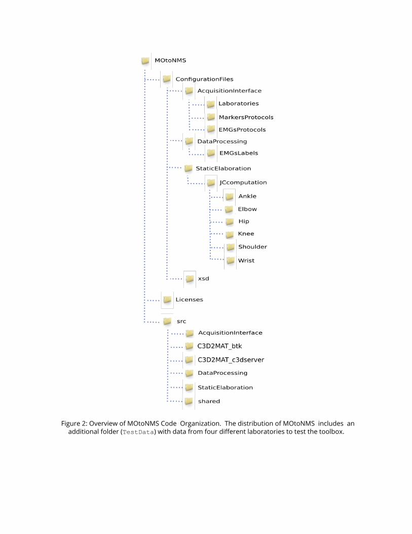
Figure 2: Overview of MOtoNMS Code Organization. The distribution of MOtoNMS includes an additional folder (TestData) with data from four different laboratories to test the toolbox.

Data OrganizationAn additional advantage of MOtoNMS is that it helps in keeping your experimental data folder well organized. Data storage is a common and important issue, especially when large amount of data are involved or when the collaboration among research teams leads to sharing of data sets and results.Thus, we have decided to force some simple rules in the storage of collected data. This allow an automatic generation of output directories with a well defined structure. Therefore, the use of MOtoNMS forces the arrangement of the processed data sets with the same structure, facilitating the retrieval of information and results and the sharing of your work with other research teams.
The only real rule that you have to follow is to place the folders of your collected data in a folder called InputData.We then encourage users to create a different folder for each acquisition, named with the date when data were collected. These folders should then be stored in another folder named with the subject identifier. Fig. 3 shows a representation of how MOtoNMS suggests to organize the data set: in black is the path of data from a single acquisition session. Inside the folder, together with the expected C3D files, you must include the acquisition.xmlfile (Fig. 3 - red) that fully describe the collected data (see Acquisition Interface).The execution of MOtoNMS automatically creates new folders (Fig. 3 - green). The new path for the output folder is created based on the input file path just replacing InputData with ElaboratedData (Ex: MyData\ElaboratedData\subjectXXX\ YearMonthDay\). Then the execution of the different tools create new subdirectories. C3D2MAT extracts data from the C3D files and stores them in mat format in the subfolder sessionData (MyData\ElaboratedData\subjectXXX\ YearMonthDay\sessionData\). staticElaborations subfolder stores the output of Static Elaboration executions. Finally the results of the multiple executions of Data Processing, with different configurations for the same input data, are stored in different subfolders, each one named with an identifier chosen by the user through the user interface (Elaboration Interface: configure your elaboration).
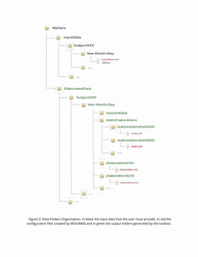
Figure 3: Data Folders Organization. In black the input data that the user must provide. In red the configuration files created by MOtoNMS and in green the output folders generated by the toolbox.

Acquisition Interface: describing your dataDuring this step a graphical user interface (GUI) will follow you in the creation of a file describing the acquisition session (acquisition.xml). This file must be created and included in the folder with the C3D data before running the next steps (Fig. 3). Furthermore, acquisition.xmlhelps when the data are shared with other researchers as they can easily figure out all the details about the acquisition session.Most of the procedure is quite simple to understand. You will go through a sequence of questions about the tracked subjects, people that collected the data, marker and EMG protocol, laboratory characteristics, etc. The only tricky thing to understand is about the prefilled setup files. Information about the laboratory setup, markers and EMG protocols are usually common to several acquisitions. Therefore, instead of writing again and again the same values for each acquisition, these data are stored in setup files that can be selected with the GUI (Fig. 4). Thus, before running the Acquisition Interface you need to have already all the necessary setup files. A few examples are available in the directories:
➢ MOtoNMS\SetupFiles\AcquisitionInterface\Laboratories (Laboratory Configurations)
➢ MOtoNMS\SetupFiles\AcquisitionInterface\MarkersProtocols(Markers Protocols)
➢ MOtoNMS\SetupFiles\AcquisitionInterface\EMGsProtocols (EMG Protocols).
If you need setup files which are not already in these folders, you can add your own setup files to these directories following the instruction provided in the sections Setup Files of the proper chapter.
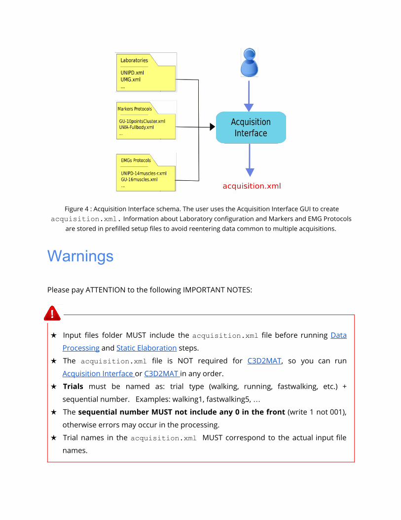
Figure 4 : Acquisition Interface schema. The user uses the Acquisition Interface GUI to create acquisition.xml. Information about Laboratory configuration and Markers and EMG Protocols
are stored in prefilled setup files to avoid reentering data common to multiple acquisitions.
Warnings
Please pay ATTENTION to the following IMPORTANT NOTES:
★ Input files folder MUST include the acquisition.xmlfile before running Data
Processing and Static Elaboration steps.
★ The acquisition.xml file is NOT required for C3D2MAT, so you can run
Acquisition Interface or C3D2MAT in any order.
★ Trials must be named as: trial type (walking, running, fastwalking, etc.) +
sequential number. Examples: walking1, fastwalking5, …
★ The sequential number MUST not include any 0 in the front (write 1 not 001),
otherwise errors may occur in the processing.
★ Trial names in the acquisition.xml MUST correspond to the actual input file
names.

★ Gait trials gathered along the negative direction of motion are not currently
supported: they may be processed without errors, but the results will not be
correct.
How to run the program
1. Set Matlab path to src\AcquisitionInterface folder
2. Run mainAcquisitionInterface.m3. Fill in the required information
mainAcquisitionInterface.m calls AcquisitionInterface.m, the core program.
Output: acquisition.xml file (saved in the input data folder).
At the beginning, the graphical interface asks if the user wants to reload an acquisition.xml file. This is a useful functionality when the user wants to start with information stored in a file already available.The resulting XML file is considered valid only when all the information are included (Appendix B: Validation of Setup and Configuration Files). However, mainAcquisitionInterface.monly requires the data which are mandatory for the following processing allowing to skip some information.
Setup filesThe following files speed up the process of compiling the acquisition.xml file that describes your acquisition session. If MOtoNMS has been already used in your laboratory to collect data with EMG and marker protocols do not go further: someone else should have already created these files. If you are not lucky and you have to write your own setup files, do not be scared: it is a simple procedure if you carefully follow the description in the next sections. Additionally, once you are done, you can check that the final XML file respect the required syntax with the validation procedure (see Appendix B: Validation of Setup and Configuration Files).

Laboratory
This XML file describes the characteristics of the laboratory where data are collected. It has been introduced to avoid re-entering same data for each acquisition carried on in the laboratory. Its name should uniquely identify the laboratory to whom it refers. Therefore, the best choice is to use a combination of laboratory name, department, university.
The following information must be included (Lst. 1):
1. Orientation of the coordinate system (<CoordinateSystemOrientation>tag, Lst.1, line 4)The coordinate system orientation refers to the global or laboratory coordinate system. We used the following convention:
- 1st axis: direction of motion- 2nd axis: vertical axis- 3rd axis: right hand rule
with the assumption that the 1st axis has the same verse of OpenSim 1st axis, i.e. it should be the positive direction of motion (Fig. 5). This convention requires that for any combination of the three axes (e.g. YZX, XZY, YXZ, etc...), the first axis must always be the direction of motion in your lab, the second one your vertical axis, and the last the one results from the right hand rule (Fig. 5) . The adopted convention follows ISB recommendation . Lst. 1 line 4 shows an example of definition of coordinate system 1
orientation.
Fig. 5 Convention for Coordinate System Orientation: example of interpretation.
Current version of MOtoNMS only manages data collected along the positive direction of motion. Gait trials gathered along the negative direction of motion may be processed without any output error, but the results will not be correct.
2. Type of force platforms (<Type> tag, Lst. 1 lines 10 and 22)Force platform (FP) type must be indicated because it influences output data (refer to The C3D File Format User Guide, by Motion Lab Systems, pag. 88
1 Ge Wu and Peter R. Cavanagh, ISB Recommendation for standardization of kinematic data in the reporting, Vol. 28 No. 10. pp. 1257-1261, 1995

http://www.projects.science.uu.nl/umpm/c3dformat_ug.pdf and to your force platform manual). MOtoNMS recognizes and processes data from force platforms of type 1, 2, 3, and 4. Each plaform returns different data as shown in the following:
● type 1: [Fx Fy Fz Px Py Mz ]
● type 2 and 4: [Fx Fy Fz Mx My Mz]
● type 3: [Fx12 Fx34 Fy14 Fy23 Fz1 Fz2 Fz3 Fz4]
where F are the measured reaction forces, M the moments, and P the center of pressure (CoP) along the three directions. Numbers in type 3 platform refers to the sensors (refer to the C3D File Format User Guide for additional information).
If your force platform includes a plate pad on the surface you need to correct CoP computation (please refer to http://www.kwon3d.com/theory/grf/pad.html for additional information). Future version of MOtoNMS will include this functionality. Please contact the authors if you need it earlier.
3. Rotation between the force platform and the global coordinates (<FPtoGlobalRotations> tag, Lst. 1, lines 12-17 and 24-33)
It is well known that each FP has its own coordinate system (Fig. 6) and that C3D files store FP data in the corresponding FP coordinate system. Therefore, the configuration file about the laboratory must provide also the transformation to rotate each FP reference system to the global one (Lst. 1, lines 12-17 and 24-33).
Figure 6: Bertec Plate Coordinate System ( from Bertec Force Plates Manual, version 1.0.0, March 2012,
http://bertec.com/uploads/pdfs/manuals/Force%20Plate%20Manual.pdf).
Lst. 1 shows an example on how to configure two Bertec force platforms. Their relative position and coordinate systems is shown in Fig. 6. Lines 12-17 (FP 1) and 24-33 (FP 2) list the required rotations. When more than one rotation is required, they are listed in

sequence and estimated around moving axes (lines 24-33).
Figure 7: FP and global coordinate systems orientation of UNIPD Laboratory.
1<Laboratory xmlns:xsi="http://www.w3.org/2001/XMLSchemainstance"> <Name>UNIPD</Name>3 <MotionCaptureSystem>BTS</MotionCaptureSystem>4 <CoordinateSystemOrientation>ZYX</CoordinateSystemOrientation> <NumberOfForcePlatforms>2</NumberOfForcePlatforms> <ForcePlatformsList> <ForcePlatform> <ID>1</ID> <Brand>Bertec</Brand>10 <Type>1</Type> <FrameRate>960</FrameRate>12 <FPtoGlobalRotations> <Rot> <Axis>X</Axis> <Degrees>90</Degrees> </Rot>17 </FPtoGlobalRotations> </ForcePlatform> <ForcePlatform>20 <ID>2</ID> <Brand>Bertec</Brand>22 <Type>1</Type> <FrameRate>960</FrameRate>24 <FPtoGlobalRotations> <Rot> <Axis>X</Axis> <Degrees>90</Degrees>

</Rot> <Rot> <Axis>Y</Axis> <Degrees>180</Degrees> </Rot>33 </FPtoGlobalRotations> </ForcePlatform> </ForcePlatformsList> </Laboratory>
Listing 1: An example of an XML file with information about the laboratory (available atSetupFiles\AcquisitionInterface\Laboratories\UNIPD.xml ).
Markers Protocols
Each marker protocol must be defined in a separate XML file. Lst. 2 shows an example where markers set for both Static (<MarkersSetStaticTrials> tag, line 3) and Dynamic Trials (<MarkersSetDynamicTrials>tag, line 4) are defined. Names of the markers must correspond to the labels used to identify the markers in the C3D files.The labels of the markers cannot include spaces as this would prevent the creation of this configuration file.
<MarkersProtocol>2 <Name>UWAFullbody</Name> <MarkersSetStaticTrials>LASI RASI LPSI RPSI … </MarkersSetStaticTrials>4 <MarkersSetDynamicTrials>C7 RACR LPSI RPSH … </MarkersSetDynamicTrials> </MarkersProtocol>
Listing 2: An example of an XML file with information about the marker protocols (available at SetupFiles\AcquisitionInterface\MarkersProtocols\UWAFullbody.xml )
EMGs Protocols
EMG protocol must be defined in an XML file. Lst. 3 shows an example including information about the name of the protocol (line 2), the list of the muscles (lines 3-10) and the instrumented leg (line 11). Muscles names (Lst. 3, lines 4-8) MUST be those assigned during the acquisition session and, therefore, must agree with labels in the C3D files.
<EMGsProtocol> <Name>UWA16musclesr</Name>

<MuscleList>4 <Muscle>Vast Lat</Muscle>
<Muscle>Gluet Max</Muscle> <Muscle>Gluet Med</Muscle> <Muscle>TFL</Muscle>
8 <Muscle>Sart</Muscle> ..... </MuscleList>11 <InstrumentedLeg>Right</InstrumentedLeg> </EMGsProtocol>
Listing 3: An example of an XML file with information about the EMG protocol (available at SetupFiles\AcquisitionInterface\EMGsProtocols\UWA16musclesr.xml).
The instrumented leg must always be defined when EMG data are collected. Depending on the leg with EMG sensors its value will be Right, Left, Both, None. These are the only acceptable strings. When EMG signals are not collected during the acquisition session, this configuration file is not required, and the user just sets at 0 the number of EMG systems on the Acquisition Interface GUI (Fig. 8).
Figure 8: Acquisition Interface: how to set the Number of EMGs System used during the acquisition.

C3DtoMAT: from C3D to MATLAB formatThis step retrieves data from the input C3D files and store them in organized MATLAB structures (.mat files). This avoid to have continuous accesses to C3D files, which are computationally expensive and redundant. Setup and configuration files are not required in this step.C3D2MAT only requires to specify the input file path. If not already available, it generates corresponding folders for the elaborated data (Folders: organize your work, MyData\ElaboratedData\subjectXXX\YearMonthDay\) and then converts all the data in mat format and stored them in the sessionData folder (MyData\ElaboratedData\subjectXXX\YearMonthDay\sessionData\). For each trial (i.e. C3D file in the input folder), a new subfolder is created with Markers (Markers.mat) , Force Platform Data (FPdata.mat) and all data stored in the analog channels (AnalogData.mat). When C3D files include events, they are converted and stored as well (Events.mat). You can add events to your C3D files using Mokka, a freely available software for biomechanical data analysis (http://b-tk.googlecode.com/svn/web/mokka/index.html), which supports many different file formats and allows to write on C3D files with a very user-friendly interface. Information common to all the trials of the session are saved in the sessionData folder. This includes markers labels of dynamic trials (dMLabels.mat), analog data labels (AnalogDataLabels.mat), force platform information (ForcePlatformInfo.mat), rates (Rates.mat), and the trials list (trialsName.mat). If any inconsistency is found, it is pointed out in the MATLAB Command Window.
Two implementations for C3D2MAT are available, one using C3Dserver software and one exploiting BTK. They return the same results, but are based on two different tools to access C3D files. You can choose among the two alternatives according to your system requirements (refer to Installation).

WarningsPlease pay ATTENTION to the following IMPORTANT NOTES:
★ Input files folder MUST be inside a folder named InputData (Folders:
organize your work).
★ The execution of C3D2MAT does not overwrite information common to the
acquisition session, i.e. that must be the same for all trials collected during an
acquisition, as trialsName.mat, Rates.mat, dMLabels, AnalogDataLabels.mat, ForcePlatformsInfo.mat. Cancel the
sessionData folder before running again the program if you add trials or
modify your data set.
★ Different events MUST have different name (Analysis Window Definition,
WindowFromC3D).
★ Events for foot strike and foot off must identify frames with non-zero force
values (Analysis Window Definition, StanceOnFPfromC3D).
★ If you are using C3D2MAT_c3dserver, remember to install C3Dserver
software (Installation) and that it works only on Matlab 32 bit.
★ If you are using C3D2MAT_btk, remember to download the correct BTK
version for your system and to add it to the path of MATLAB. Type the
command help btkin the Matlab’s command window to verify that BTK is
loaded in MATLAB (Installation).
★ Data gathered using FP of type 4 are stored in the C3D files in V
(http://www.c3d.org/pdf/c3dformat_ug.pdf). C3D2MAT retrieves and directly
converts force data in N and N*mm or N*m (according to the used distance
unit). Be aware that the scale of results saved in FPdata.mat does not match
with the one you see in the input C3D files.
★ C3D files storing data gathered with FPs of type 4 must include information
about the corresponding FP calibration matrix. This is required to convert
force data from V to N and N*mm or N*m.

How to run the program
1. Set Matlab path on src\C3D2MAT_btk (or C3D2MAT_c3dserver) folder
2. Run C3D2MAT.m3. Select your C3D input data folder
Output: data from C3D files in the specified data folder are converted and saved in mat format.

Data Processing: elaborate your dynamic trialsStarting from motion data stored as MATLAB structures by C3DtoMAT, Data Processing (Fig. 9) produces .trc and .mot files for OpenSim, storing respectively markers and forces information. When collected, it also processes EMG signals. Data Processing is only responsible for handling dynamic trials, static trials are managed by Static Elaboration.
Markers and Ground Reaction Forces ElaborationThis section provides a description of the elaboration steps for marker trajectories and ground reaction forces (Fig. 9 - left column). At first, markers trajectories undergo piecewise cubic interpolation to fill any possible gap; a text file (InterpolationNote.txt) with information about the procedure is also saved. Interpolation is executed in the range between the first and last frames where marker occurs, while the values outside this range are set to zero. The Analog Data Splitting step (Fig. 9) handles GRF data generated by the most common force plate types (http://www.projects.science.uu.nl/umpm/c3dformat_ug.pdf). First, the plate moments and centers of pressure are computed with different procedure depending on the FP type and its output. Then, the pre-processed marker data and raw GRFs are filtered with a zero-lag second order low pass butterworth filter at customizable cut-off frequencies (Elaboration Interface: configure your elaboration). The analysis window definition sub-block (Fig. 9) selects the portion of the data to be processed. Different methods are available and described in a dedicated section (Analysis WIndow Definition).At this step, plots of the computed values (i.e., raw EMG, envelopes, and raw and filtered forces, CoP, and moments) are stored for offline visual inspection.Processed GRFs are used to compute free torques based on filtered forces, moments and CoP for the selected frames. Finally, marker and GRF data are projected from laboratory or FP reference system to the global reference system of the selected musculoskeletal application, i.e. OpenSim. Required rotations depend in the laboratory setup described in the Laboratory setup file.

Figure 9: Flowchart of steps in the Data Processing part.

EMG ProcessingWhen available, EMG signals are also processed for EMG-driven neuromusculoskeletal applications. Currently, MOtoNMS supports CEINMS input format (https://simtk.org/home/ceinms) but the text file can be easily adapted to other applications. A subset of all the acquired muscles can be selected. Maximum value for each EMG signal is estimated from one or more trials defined by the user: when available, a trial of maximal voluntary isometric contraction can be used, as well as a subset of the input trials. Envelopes for the EMGs are computed and then normalized with their estimated maximum value. Obtained normalized envelopes are stored in a text file (emg.txt) according to CEINMS input file format (https://simtk.org/home/ceinms), with output labels that can be defined by the user (for details refer to Setup Files in this chapter).
Elaboration Interface: configure your elaborationThe execution of Data Processing block is univocally defined by a set of parameters selected by the user. All these parameters are saved in the elaboration.xml configuration file (Lst. 4), which guarantees the high configurability and the fully reproducibility of the toolbox behavior.This configuration file can be obtained running a user-friendly graphical interface (GUI). The first thing the GUI will ask is to select the input data folder and next to enter an identificator for the current elaboration (Fig. 10). The identificator will be used to name a new folder in ElaboratedData storing the results of this elaboration (e.g. elaboration01ID and elaboration02ID in Fig. 3, Folders: organize your work).
Figure 10 : Elaboration Interface: setting the Elaboration Identificator.
Then, the GUI will ask you the parameters required for the elaboration, which are briefly described in the following:
● Trials to be processed: a subset of the C3D files in the input folder
● Cutoff frequency for markers filtering specified for each trial type (walking,
running,...) (Optional)
● Cutoff frequency for force filtering specified for each trial type (walking, running,..)
(Optional)
● Cutoff frequency for CoP filtering depending on FP type (Optional)
● Analysis Window Computation method, with its own parameters (offset, C3D
events labels, frames for the manual method). Available methods are further
described in a dedicated section (Analysis Window Definition)
● List of markers to be written in .trc file
When EMG data are available:
● Trials for the computation of the maximum value of EMG signals
● Muscles to be considered in the processing (a subset of the acquired EMGs).
● EMG output labels. Different application names EMG signals differently. To avoid
typing output labels several times, translation between EMG protocol labels (in
C3D files) and application labels is stored in a setup file (see EMGs Labels) that
can be selected from the GUI.
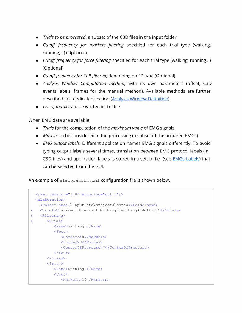
An example of elaboration.xml configuration file is shown below.
<?xml version="1.0" encoding="utf8"?> <elaboration> <FolderName>.\InputData\subjectX\dateX</FolderName>4 <Trials>Walking1 Running1 Walking3 Walking4 Walking5</Trials>5 <Filtering>6 <Trial> <Name>Walking1</Name> <Fcut> <Markers>8</Markers> <Forces>8</Forces> <CenterOfPressure>7</CenterOfPressure> </Fcut> </Trial> <Trial> <Name>Running1</Name> <Fcut> <Markers>10</Markers>

<Forces>10</Forces> <CenterOfPressure>7</CenterOfPressure> </Fcut> </Trial> .... </Filtering>
25 <WindowSelectionProcedure>26 <StanceOnFPfromC3D> <Leg>Right</Leg>28 <LabelForHeelStrike>Foot Strike</LabelForHeelStrike> <LabelForToeOff>Foot Off</LabelForToeOff>30 <Offset>20</Offset> </StanceOnFPfromC3D> </WindowSelectionProcedure>
34 <Markers>C7 RA LA L5 RPSIS LPSIS RASIS LASIS RGT LGT RLE ... </Markers>
36 <EMGMaxTrials>Walking1 Walking2 Walking3 Walking4</EMGMaxTrials>
38 <EMGsSelection> <EMGSet>UNIPDCEINMS</EMGSet> <EMGs> <EMG> <OutputLabel>addmag_r</OutputLabel> <C3DLabel>Right Adductor Longus</C3DLabel> </EMG> ... </EMGs> </EMGsSelection>49 <EMGOffset>0.2</EMGOffset> </elaboration>
Listing 4: Example of an elaboration.xml
The only parameter that cannot be modified by the GUI is the EMGOffset(Lst. 4, line 49). MOtoNMS stores the EMG values starting EMGOffsetsecond before the initial frame. While MOtoNMS has not been designed to synchronize markers, ground reaction forces and EMGs, it accounts for the need of follow-up applications to deal with the electromechanical delay of muscles providing EMG data from an anterior offset in time. Default value is set to 0.2 seconds. This setting does not allow to define analysis windows starting at the first frame. If you do not need to consider the electromechanical delay in your research, you can manually set EMGOffsetto 0 in your elaboration.xml file. This also enables the elaboration of data from the first frame.

Analysis Window Definition
Different methods to define the analysis window are available. If events are stored in C3D files, they may be selected as start and end frames of the analysis, otherwise desired frames can be inserted manually. An automatic detection of gait events is also possible based on a thresholding algorithm based on force plate data . The following 2
explains the available methods with additional details.
ComputeStancePhase: automatic detection of stance phase using a thresholding algorithm based on force plate data. This method needs only to know the leg of the stance. When only one leg is instrumented (see EMGs Protocols), this information can be automatically obtained from the acquisition.xml file. When both legs are instrumented, the user is asked to indicate the leg he/she wants to consider. Once that the leg is defined, the stance phase is selected based on force data from the FP struck by this leg (Lst. 5, line 3). It is also possible to add an offset to the stance phase such that the analysis window will start offset frames before the heel strike and end offset frames after the toe off (Lst. 5, line 2).
1 <ComputeStancePhase> <Offset>20</Offset>3 <Leg>Right</Leg> </ComputeStancePhase>
Listing 5: Example of ComputeStancePhase tag in an elaboration.xml file
StanceOnFPfromC3D: method for the selection of analysis window based on events stored in C3D files. It looks for the windows defined by the selected events and chooses the one when the instrumented leg struck the force plate. Events must be specified by the user and correspond to the label used in the C3D files (Elaboration Interface: configure your elaboration). Instrumented leg can be selected from the EMG protocol (EMGs Protocols, Lst. 3, line 11) or defined by the user when both limbs are instrumented.Events must precisely define the stance window: MOtoNMS checks force platform values to ensure the validity of the events on the C3D files and errors may be raised. Finally, this method allows to add an offset to the selected events to consider a wider analysis window (Lst. 6, line 5).
2 Rueterbories J et al., Medical Engineering & Physics 32: 545-552, 2010
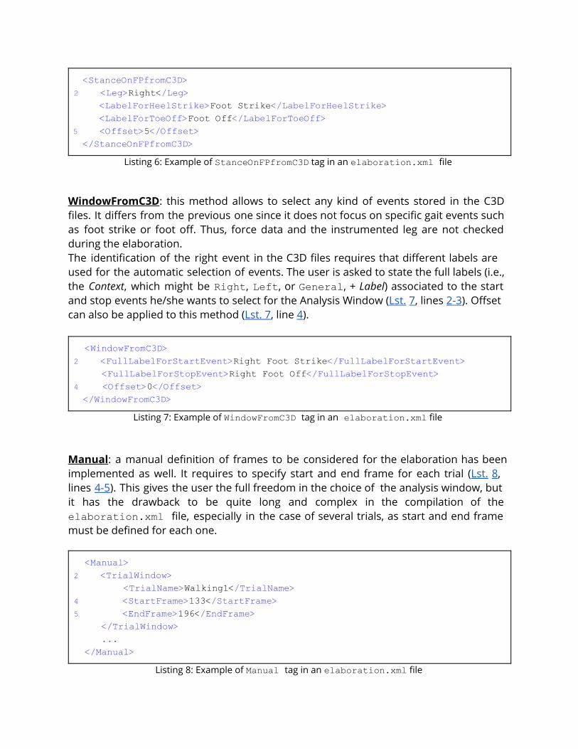
<StanceOnFPfromC3D>2 <Leg>Right</Leg> <LabelForHeelStrike>Foot Strike</LabelForHeelStrike> <LabelForToeOff>Foot Off</LabelForToeOff>5 <Offset>5</Offset> </StanceOnFPfromC3D>
Listing 6: Example of StanceOnFPfromC3D tag in an elaboration.xml file
WindowFromC3D: this method allows to select any kind of events stored in the C3D files. It differs from the previous one since it does not focus on specific gait events such as foot strike or foot off. Thus, force data and the instrumented leg are not checked during the elaboration. The identification of the right event in the C3D files requires that different labels are used for the automatic selection of events. The user is asked to state the full labels (i.e., the Context, which might be Right, Left, or General, + Label) associated to the start and stop events he/she wants to select for the Analysis Window (Lst. 7, lines 2-3). Offset can also be applied to this method (Lst. 7, line 4).
<WindowFromC3D>2 <FullLabelForStartEvent>Right Foot Strike</FullLabelForStartEvent> <FullLabelForStopEvent>Right Foot Off</FullLabelForStopEvent>4 <Offset>0</Offset> </WindowFromC3D>
Listing 7: Example of WindowFromC3D tag in an elaboration.xml file
Manual: a manual definition of frames to be considered for the elaboration has been implemented as well. It requires to specify start and end frame for each trial (Lst. 8, lines 4-5). This gives the user the full freedom in the choice of the analysis window, but it has the drawback to be quite long and complex in the compilation of the elaboration.xml file, especially in the case of several trials, as start and end frame must be defined for each one.
<Manual>2 <TrialWindow> <TrialName>Walking1</TrialName>4 <StartFrame>133</StartFrame>5 <EndFrame>196</EndFrame> </TrialWindow> ... </Manual>
Listing 8: Example of Manual tag in an elaboration.xml file
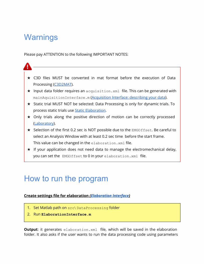
Warnings
Please pay ATTENTION to the following IMPORTANT NOTES:
★ C3D files MUST be converted in mat format before the execution of Data
Processing (C3D2MAT).
★ Input data folder requires an acquisition.xml file. This can be generated with
mainAquisitionInterface.m (Acquisition Interface: describing your data).
★ Static trial MUST NOT be selected: Data Processing is only for dynamic trials. To
process static trials use Static Elaboration.
★ Only trials along the positive direction of motion can be correctly processed
(Laboratory).
★ Selection of the first 0.2 sec is NOT possible due to the EMGOffset. Be careful to
select an Analysis Window with at least 0.2 sec time before the start frame.
This value can be changed in the elaboration.xml file.
★ If your application does not need data to manage the electromechanical delay,
you can set the EMGOffset to 0 in your elaboration.xml file.
How to run the program
Create settings file for elaboration (Elaboration Interface)
1. Set Matlab path on src\DataProcessing folder
2. Run ElaborationInterface.m
Output: it generates elaboration.xml file, which will be saved in the elaboration folder. It also asks if the user wants to run the data processing code using parameters
from the elaboration.xml file just created.
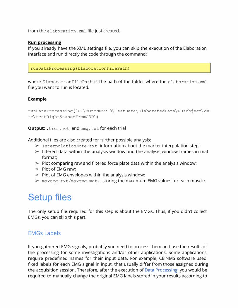
Run processingIf you already have the XML settings file, you can skip the execution of the Elaboration Interface and run directly the code through the command:
runDataProcessing(ElaborationFilePath)
where ElaborationFilePathis the path of the folder where the elaboration.xml file you want to run is located.
Example
runDataProcessing(‘C:\MOtoNMSv10\TestData\ElaboratedData\GUsubject\date\testRightStanceFromC3D’)
Output: .trc, .mot, and emg.txt for each trial
Additional files are also created for further possible analysis:➢ InterpolationNote.txt information about the marker interpolation step;➢ filtered data within the analysis window and the analysis window frames in mat
format; ➢ Plot comparing raw and filtered force plate data within the analysis window;➢ Plot of EMG raw; ➢ Plot of EMG envelopes within the analysis window;➢ maxemg.txt/maxemg.mat, storing the maximum EMG values for each muscle.
Setup filesThe only setup file required for this step is about the EMGs. Thus, if you didn’t collect EMGs, you can skip this part.
EMGs Labels
If you gathered EMG signals, probably you need to process them and use the results of the processing for some investigations and/or other applications. Some applications require predefined names for their input data. For example, CEINMS software used fixed labels for each EMG signal in input, that usually differ from those assigned during the acquisition session. Therefore, after the execution of Data Processing, you would be required to manually change the original EMG labels stored in your results according to

the needs of CEINMS or any other application you want to use. MOtoNMS allows you to avoid this tedious manual process, and does it for you. The toolbox can save results changing EMG labels coming from the acquisition (stored in the C3D files) in those desidered by the user. You just have to specify the labels you need in your results, and the emg.txt output file will be saved using them.However, you are not asked to input this information, usually common for a set of elaboration, each time you are running the Elaboration Interface GUI. It would be time consuming, boring and therefore error prone, especially considering the number of EMG signals that can be acquired during an acquisition. Instead, this association between EMG labels stored in C3D files and those required for an application is defined in a XML setup file, that can be selected through the GUI.This file MUST be saved in SetupFiles\DataProcessing\EMGsLabels\and named with the sequence of EMG protocol and application names. (e.g., UWACEINMS.xml). The name stands for the EMG labels collected in a certain laboratory that must be translated in those required for a certain application.An example of how to compile it is shown in Lst. 9. You have to manually edit this file but it is fairly easy and you can check your file with respect to the required syntax with the validation procedure (see Appendix B: Validation of Setup and Configuration Files).
<EMGSet>2 <EMG>3 <OutputLabel>addmag_r</OutputLabel>4 <C3DLabel>Add Magnus</C3DLabel> </EMG> <EMG> <OutputLabel>bicfemlh_r</OutputLabel> <C3DLabel>Biceps Fem</C3DLabel> </EMG> .......
</EMGSet>Listing 9: Example of setup file for EMG processing:
SetupFiles\DataProcessing\EMGsLabels\UWACEINMS.xml

Static Elaboration: process your static trialsOpenSim requires static trials for the scaling procedure (http://simtk-confluence.stanford.edu:8080/display/OpenSim/Getting+Started+with+Scaling). The objective of the elaboration of these trials is to produce for each static trial a markers trajectories file (.trc), optimized for the Scaling in OpenSim.Starting from the mat structures created by C3D2MAT, Static Elaboration apply the same filter procedure used in Data Processing. The main step is then joint centers (JC) estimation. These are points required to improve the accuracy of the OpenSim scaling procedure.In the current toolbox version, methods for hip (HJC), knee (KJC), ankle (AJC), elbow (EJC), shoulder (SJC) and wrist (WJC) joint centers computation are available. More specifically, HJC can be assessed exploiting Harrington , while the others can be 3
computed as the mid points between anatomical landmarks specified in the corresponding setup files (Setup Files). However, the structure of the software intentionally allows an easy integration of other algorithms for both lower and upper limbs joints. The resulting trajectories are then added to the markers list defined by the user (Static Interface: configure your elaboration). The updated list is finally rotated into OpenSim reference system and stored in the output .trc file.
Static Interface: configure your elaborationAs Data Processing (Elaboration Interface: configure your elaboration), the execution of the Static Elaboration block is fully defined by a set of parameters selected by the user.All these parameters are enclosed in the static.xmlconfiguration file (Lst. 10), which can be obtained running a graphical user interface.The GUI will ask first to select the input data folder and next to enter an identifier for the current elaboration. The identifier will be used to name the new folder storing the results of this elaboration (e.g. staticelaboration01ID, staticelaboration02ID in Fig. 3, Folders: organize your work). As shown in Fig. 3, all static elaborations are grouped in the staticElaborationfolder to avoid confusion with the output folders of Data Processing.Then, the GUI will ask the user the parameters required for the elaboration, which are briefly described in the following:
3 Harrington ME, et al., Journal of Biomechanics,Biomechanics 40:595–602, 2007

● Static trial to be processed
● Cutoff frequency for markers filtering (Optional)
● Joints for center computation
● Methods for the computation of the joint centers, which are defined selecting the
corresponding setup file (Setup Files)
● List of markers to be written in .trc file
An example of static.xml configuration file is shown in Lst. 10. Before going into details about this file we need to give you some additional information about JC computation. Different methods for the computation of the different JC may require different input data. Usually these input data includes the markers position during the static acquisition. However, different marker protocols use different labels to identify the same body landmark. Thus, it is necessary to define the connection between the marker required by a method (i.e. the left and right anterior and posterior superior iliac spine for the Harrington method) and their names according to the markers protocol used for the data collection. As it would be too complex and error prone to do it for each elaboration, this information is stored in a setup file (see Setup Files in this chapter), one for each JC computational method. Each file describes how the landmarks of interested are named in different marker protocols. A user can add new protocols to the file when required.
Static Elaboration retrieved from the Setup File of the selected JC computation method the marker labels in the marker protocol used in the static trial selected for the processing and save them in the static.xml file (Lst. 10, lines 12-16, 24-28 and 36-39). The list of markers to be stored in the .trc file (Lst. 10, line 44) MUST NOT include the estimated JC labels, as it will be automatically updated.
<?xml version="1.0" encoding="utf8"?> <static> <FolderName>.\InputData\MassSart\2010\</FolderName>4 <TrialName>Static1</TrialName>5 <Fcut>8</Fcut>6 <JCcomputation> <Joint> <Name>Ankle</Name>9 <Method>AJCMidPoint</Method>10 <Input> <MarkerNames> <Marker>LLMAL</Marker> <Marker>RLMAL</Marker> <Marker>LMMAL</Marker>

<Marker>RMMAL</Marker> </MarkerNames> </Input> </Joint>19 <Joint> <Name>Hip</Name> <Method>HJCHarrington</Method> <Input> <MarkerNames> <Marker>LASI</Marker> <Marker>RASI</Marker> <Marker>LPSI</Marker> <Marker>RPSI</Marker> </MarkerNames> </Input> </Joint>31 <Joint> <Name>Knee</Name> <Method>KJCMidPoint</Method> <Input> <MarkerNames> <Marker>LeLFC</Marker> <Marker>RiLFC</Marker> <Marker>LeMFC</Marker> <Marker>RiMFC</Marker> </MarkerNames> </Input> </Joint> </JCcomputation>44 <trcMarkers>C7 CLAV LACR LASH LPSH LUA1 LUA2 LUA3 ....</trcMarkers> </static>
Listing 10: Example of a static.xml
Warnings Please pay ATTENTION to the following IMPORTANT NOTES:
★ For any JC computation method, a setup file MUST be predefined (see Setup
Files).
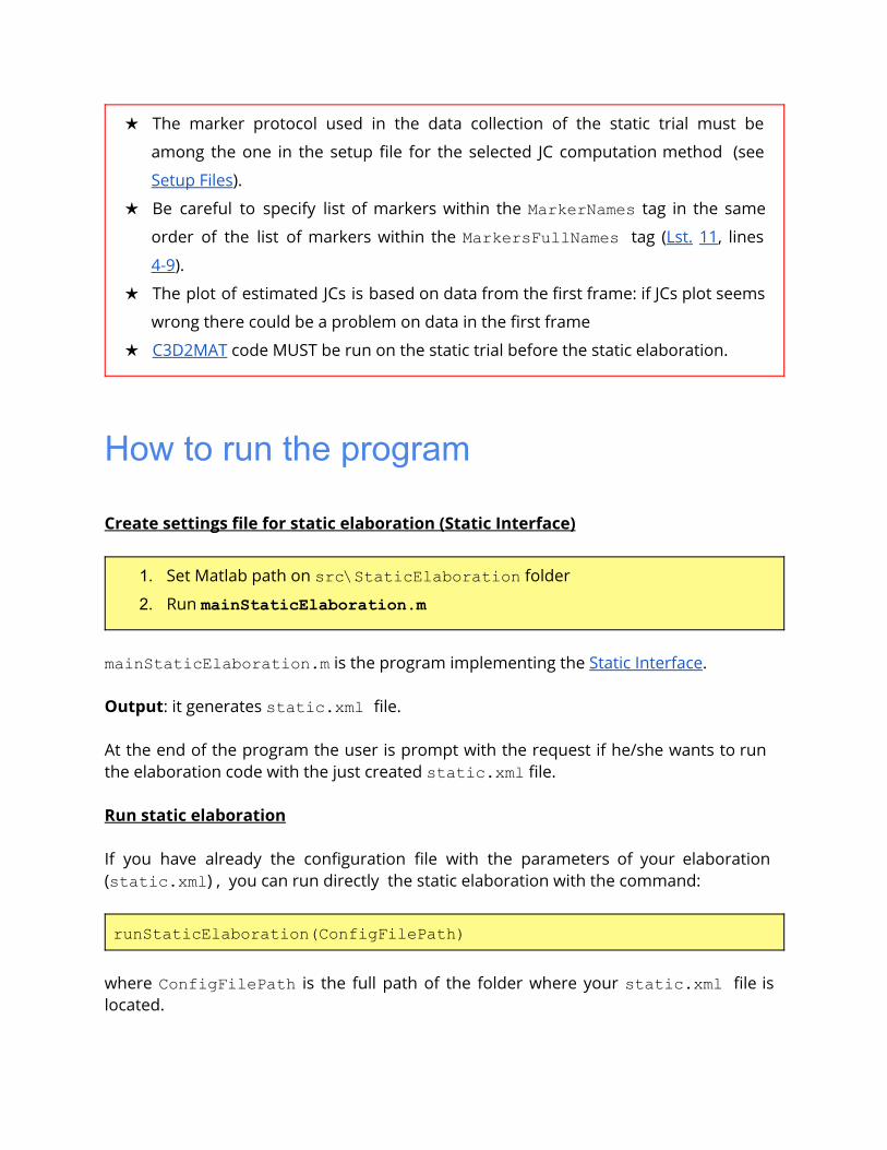
★ The marker protocol used in the data collection of the static trial must be
among the one in the setup file for the selected JC computation method (see
Setup Files).
★ Be careful to specify list of markers within the MarkerNamestag in the same
order of the list of markers within the MarkersFullNames tag (Lst. 11, lines
4-9).
★ The plot of estimated JCs is based on data from the first frame: if JCs plot seems
wrong there could be a problem on data in the first frame
★ C3D2MAT code MUST be run on the static trial before the static elaboration.
How to run the program
Create settings file for static elaboration (Static Interface)
1. Set Matlab path on src\StaticElaboration folder
2. Run mainStaticElaboration.m
mainStaticElaboration.m is the program implementing the Static Interface.
Output: it generates static.xml file.
At the end of the program the user is prompt with the request if he/she wants to run the elaboration code with the just created static.xml file.
Run static elaboration
If you have already the configuration file with the parameters of your elaboration (static.xml) , you can run directly the static elaboration with the command:
runStaticElaboration(ConfigFilePath)
where ConfigFilePathis the full path of the folder where your static.xml file is located.
Output: static.trc, with the processed markers trajectories and the computed JC
Additional files are also generated to help in validation of obtained results:➢ computed joint centers coordinate in .mat format➢ plot of estimated JCs
Setup FilesThe main information that the user have to define for a static elaboration is the joint centers he/she is interested in computing, the methods to be used for their computation and the parameters each method requires. The last one might be very long and error prone to be edited at each elaboration, so we decided that it would be easier to enclose this parameters in a setup file. The Static Interface will thus ask you to select a setup file for each JC computation. The following explains how to fill these setup files.
Joint Center Computation Methods
Each implemented JC computation method requires a file that list how the required input markers are labelled in each marker protocol. This file MUST be saved in SetupFiles\StaticElaboration\JCcomputation\ within the folder of the corresponding joint, as shown in Fig. 11. While not mandatory, our suggestion is to name the file with the acronym of the joint name followed by the identifier of the JC computation method. When only a method is available for a joint, the Static Interface will not ask to choose the setup file and select the only one available in the folder.
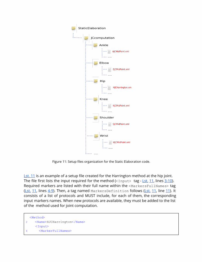
Figure 11: Setup files organization for the Static Elaboration code.
Lst. 11 is an example of a setup file created for the Harrington method at the hip joint. The file first lists the input required for the method (<Input> tag - Lst. 11, lines 3-10). Required markers are listed with their full name within the <MarkersFullNames>tag (Lst. 11, lines 4-9). Then, a tag named MarkersDefinitionfollows (Lst. 11, line 11). It consists of a list of protocols and MUST include, for each of them, the corresponding input markers names. When new protocols are available, they must be added to the list of the method used for joint computation.
<Method>2 <Name>HJCHarrington</Name> <Input>4 <MarkerFullNames>

<Marker>Left Anterior Superior Iliac Spine</Marker> <Marker>Right Anterior Superior Iliac Spine</Marker> <Marker>Left Posterior Superior Iliac Spine</Marker> <Marker>Right Posterior Superior Iliac Spine</Marker> </MarkerFullNames> </Input>11 <MarkersDefinition>12 <Protocol>
<Name>UWAFullbody</Name> <MarkerNames>
15 <Marker>LASI</Marker> <Marker>RASI</Marker> <Marker>LPSI</Marker> <Marker>RPSI</Marker>
</MarkerNames> </Protocol>
21 <Protocol> <Name>UNIPDALclusters</Name>
<MarkerNames> <Marker>LASIS</Marker> <Marker>RASIS</Marker> <Marker>LPSIS</Marker> <Marker>RPSIS</Marker> </MarkerNames> </Protocol> ... 30 </MarkersDefinition> </Method>
Listing 11: Example of setup file for the Harrington method: SetupFiles\StaticElaboration\JCcomputation\Hip\HJCHarrington.xml

Error MessagesA complete section dedicated to handled error messages will be available in the next version of this User Manual.Meanwhile, for any doubt or problem, please write an email to Alice Mantoan, [email protected]

Appendix A: Setup FilesThis appendix lists the setup files already available in MOtoNMS distribution. They are stored in MOtoNMS\SetupFiles\ folder (Fig. 2 Code Organization). They are selected by the users through the GUIs to create the configuration files (acquisition.xml, elaboration.xml and static.xml) required for processing.
Acquisition Interface Laboratories
● UNIPD.xml● UMG.xml● GU.xml● UWA.xml
Markers Protocols● UNIPDALclusters.xml● GU10pointsCluster.xml● UMGOpenSim.xml● UWAFullbody.xml
EMGs Protocols● UNIPD14musclesr.xml● GU16muscles.xml● UWA16musclesr.xml
Data Processing EMGsLabels
● UNIPDCEINMS.xml● GUCEINMS.xml● UWACEINMS.xml
Static Elaboration JCcomputation
Ankle● AJCMidPoint.xml
Elbow● EJCMidPoint.xml

Hip
● HJCHarrington.xml
Knee● KJCMidPoint.xml
Shoulder● SJCMidPoint.xml
Wrist● WJCMidPoint.xml

Appendix B: Validation of Setup and Configuration FilesThis section is only for people that needs to create new setup files, or want to manually change their configuration files. Please, try to use the graphical user interfaces and avoid playing directly with the XML configuration files. It took us a lot of time to implement them, therefore make us happy and use them :).
The only real reason to play directly with the XML files is when you start doing something new: (1) setup a new laboratory, or a new protocol either for (2) EMGs or (3) makers or (4) you need different output labels for your processed EMGs, or maybe you want to introduce a new way to (5) compute joint center. In all these case, you need to manually create new setup files.
Usually these XML files are really simple and you can copy one already available and easily understand what you need to change. But when you are done, it is a good practice to check the syntax of your XML file against the grammar. Again, as it took us quite a lot to develop a grammar for each possible XML file, please make us happy and use it. Additionally, this is also really helpful for you as you can be sure that your file is syntactically correct and ready to be used in MOtoNMS. Indeed, errors in editing the setup files result in execution errors when running the source code; these may not be easy to understand if you are not an expert of MATLAB language and MOtoNMS behavior.
There are many possible tools that you can use. We just suggest a couple of the easiest to be used because everything is online and you do not have to install anything on your computer.
Choose one of the following links: http://www.freeformatter.com/xml-validator-xsd.html http://www.corefiling.com/opensource/schemaValidate.html
and upload your XML file and the corresponding XML Schema (the .xsd file).The following tables are listing the XML Schema for each type of XML setup and configuration files that you find in MOtoNMS.
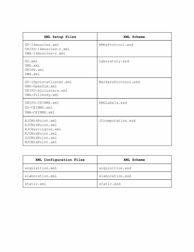
XML Setup Files XML SchemeGU16muscles.xmlUNIPD14musclesr.xmlUWA16musclesr.xml
EMGsProtocol.xsd
GU.xmlUMG.xmlUNIPD.xmlUWA.xml
Laboratory.xsd
GU10pointsCluster.xmlUMGOpenSim.xmlUNIPDALclusters.xmlUWAFullbody.xml
MarkersProtocol.xsd
UNIPDCEINMS.xmlGUCEINMS.xmlUWACEINMS.xml
EMGLabels.xsd
AJCMidPoint.xmlEJCMidPoint.xmlHJCHarrington.xmlKJCMidPoint.xmlSJCMidPoint.xmlWJCMidPoint.xml
JCcomputation.xsd
XML Configuration Files XML Schemeacquisition.xml acquisition.xsd
elaboration.xml elaboration.xsd
static.xml static.xsd

Appendix C: Revision Historyv. 1.0 (February 17, 2014)
Initial Release
v. 1.1 (March 11, 2014)
Added Features EMG selection based on Analog Labels from each C3D input file Added shoulder, elbow, and wrists JC, and setup files for Griffith University markerset Implemented C3D2MAT processing step using BTK to avoid C3Dserver platform constrain (Matlab 32 bit on Windows)
Restructuring Added src/shared folder to store functions common to several steps
Other Changes Added memory of last path when selecting files from graphical user interfaces (GUIs) Removed warning messages caused by the lack of subject's first and last names when loading a predefined acquisition.xml
Bug Fixes When running a predefined elaboration.xml, the GUIs asked for a new elaboration identifier that won't be used. Modified popup order in Elaboration and Static Interface: now user is asked to choose what to do (set a new elaboration, load and modify an old one or run one previously defined), and only after to insert the new elaboration identifier if it is the case.