Motion Estimation I - courses.cs.washington.edu · 5/9/2011 1 Motion Estimation (I) Ce Liu [email protected] Microsoft Research New England We live in a moving world • Perceiving,

5/9/2011

1

Motion Estimation (I)

Ce Liu

[email protected]

Microsoft Research New England

We live in a moving world

• Perceiving, understanding and predicting motion is an important part of our daily lives

Motion estimation: a core problem of computer vision

• Related topics: – Image correspondence, image registration, image matching, image

alignment, …

• Applications

– Video enhancement: stabilization, denoising, super resolution

– 3D reconstruction: structure from motion (SFM)

– Video segmentation

– Tracking/recognition

– Advanced video editing

Contents (today)

• Motion perception

• Motion representation

• Parametric motion: Lucas-Kanade

• Dense optical flow: Horn-Schunck

• Robust estimation

• Applications (1)

5/9/2011

2

Readings

• Rick’s book: Chapter 8

• Ce Liu’s PhD thesis (Appendix A & B)

• S. Baker and I. Matthews. Lucas-Kanade 20 years on: a unifying framework. IJCV 2004

• Horn-Schunck (wikipedia)

• A. Bruhn, J. Weickert, C. Schnorr. Lucas/Kanade meets Horn/Schunk: combining local and global optical flow methods. IJCV 2005

Contents







Seeing motion from a static picture?

http://www.ritsumei.ac.jp/~akitaoka/index-e.html

More examples

5/9/2011

3

How is this possible?

• The true mechanism is to be revealed

• FMRI data suggest that illusion is related to some component of eye movements

• We don’t expect computer vision to “see” motion from these stimuli, yet

What do you see?

In fact, … The cause of motion

• Three factors in imaging process – Light

– Object

– Camera

• Varying either of them causes motion – Static camera, moving objects (surveillance)

– Moving camera, static scene (3D capture)

– Moving camera, moving scene (sports, movie)

– Static camera, moving objects, moving light (time lapse)

5/9/2011

4

Motion scenarios (priors)

Static camera, moving scene Moving camera, static scene

Moving camera, moving scene Static camera, moving scene, moving light

We still don’t touch these areas

Motion analysis: human vs. computer

• Challenges of motion estimation – Geometry: shapeless objects

– Reflectance: transparency, shadow, reflection

– Lighting: fast moving light sources

– Sensor: motion blur, noise

• Key: motion representation – Ideally, solve the inverse rendering problem for a video sequence

• Intractable!

– Practically, we make strong assumptions

• Geometry: rigid or slow deforming objects

• Reflectance: opaque, Lambertian surface

• Lighting: fixed or slow changing

• Sensor: no motion blur, low-noise

Contents







5/9/2011

5

Parametric motion

• Mapping: 𝑥1, 𝑦1 → (𝑥2, 𝑦2) – (𝑥1, 𝑦1): point in frame 1

– (𝑥2, 𝑦2): corresponding point in frame 2

• Global parametric motion: 𝑥2, 𝑦2 = 𝑓(𝑥1, 𝑦1; 𝜃)

• Forms of parametric motion

– Translation: 𝑥2𝑦2=𝑥1 + 𝑎𝑦1 + 𝑏

– Similarity: 𝑥2𝑦2= 𝑠

cos 𝛼 sin 𝛼

− sin 𝛼 cos 𝛼

𝑥1 + 𝑎𝑦1 + 𝑏

– Affine: 𝑥2𝑦2=𝑎𝑥1 + 𝑏𝑦1 + 𝑐𝑑𝑥1 + 𝑒𝑦1 + 𝑓

– Homography: 𝑥2𝑦2=1

𝑧

𝑎𝑥1 + 𝑏𝑦1 + 𝑐𝑑𝑥1 + 𝑒𝑦1 + 𝑓

, 𝑧 = 𝑔𝑥1 + 𝑕𝑦1 + 𝑖

Parametric motion forms

Translation

Homography

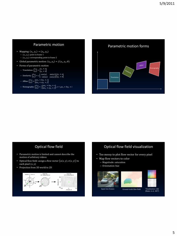
Optical flow field

• Parametric motion is limited and cannot describe the motion of arbitrary videos

• Optical flow field: assign a flow vector 𝑢 𝑥, 𝑦 , 𝑣 𝑥, 𝑦 to

each pixel (𝑥, 𝑦)

• Projection from 3D world to 2D

Optical flow field visualization

• Too messy to plot flow vector for every pixel

• Map flow vectors to color

– Magnitude: saturation

– Orientation: hue

Ground-truth flow field Visualization code

[Baker et al. 2007]

Input two frames

5/9/2011

6

Matching criterion

• Brightness constancy assumption

𝐼1 𝑥, 𝑦 = 𝐼2 𝑥 + 𝑢, 𝑦 + 𝑣 + 𝑛

𝑛 ∼ 𝑁 0, 𝜎2

• Noise 𝑛

• Matching criteria – What’s invariant between two images?

• Brightness, gradients, phase, other features…

– Distance metric (L2, robust functions)

𝐸 𝑢, 𝑣 = 𝐼1 𝑥, 𝑦 − 𝐼2 𝑥 + 𝑢, 𝑦 + 𝑣2

𝑥,𝑦

– Correlation, normalized cross correlation (NCC)

Contents







Problem definition: optical flow

How to estimate pixel motion from image H to image I?

• Solve pixel correspondence problem

– given a pixel in H, look for nearby pixels of the same color in I

Key assumptions

• color constancy: a point in H looks the same in I

– For grayscale images, this is brightness constancy

• small motion: points do not move very far

This is called the optical flow problem

Optical flow constraints (grayscale images)

Let’s look at these constraints more closely

• brightness constancy: Q: what’s the equation?

• small motion: (u and v are less than 1 pixel)

– suppose we take the Taylor series expansion of I:

5/9/2011

7

Optical flow equation

Combining these two equations

Optical flow equation

Combining these two equations

In the limit as u and v go to zero, this becomes exact

Lucas-Kanade flow

How to get more equations for a pixel?

• Basic idea: impose additional constraints

– most common is to assume that the flow field is smooth locally

– one method: pretend the pixel’s neighbors have the same (u,v)

» If we use a 5x5 window, that gives us 25 equations per pixel!

RGB version

How to get more equations for a pixel?

• Basic idea: impose additional constraints

– most common is to assume that the flow field is smooth locally

– one method: pretend the pixel’s neighbors have the same (u,v)

» If we use a 5x5 window, that gives us 25*3 equations per pixel!

5/9/2011

8

Lucas-Kanade flow

Prob: we have more equations than unknowns

• The summations are over all pixels in the K x K window

• This technique was first proposed by Lucas & Kanade (1981)

Solution: solve least squares problem

• minimum least squares solution given by solution (in d) of:

Conditions for solvability

• Optimal (u, v) satisfies Lucas-Kanade equation

When is This Solvable? • ATA should be invertible

• ATA should not be too small due to noise

– eigenvalues l1 and l2 of ATA should not be too small

• ATA should be well-conditioned

– l1/ l2 should not be too large (l1 = larger eigenvalue)

Does this look familiar? • ATA is the Harris matrix

Observation

This is a two image problem BUT • Can measure sensitivity by just looking at one of the images!

• This tells us which pixels are easy to track, which are hard

– very useful for feature tracking...

Errors in Lucas-Kanade

What are the potential causes of errors in this procedure?

• Suppose ATA is easily invertible

• Suppose there is not much noise in the image

When our assumptions are violated

• Brightness constancy is not satisfied

• The motion is not small

• A point does not move like its neighbors

– window size is too large

– what is the ideal window size?

5/9/2011

9

• Can solve using Newton’s method

– Also known as Newton-Raphson method

– For more on Newton-Raphson, see (first four pages)

» http://www.ulib.org/webRoot/Books/Numerical_Recipes/bookcpdf/c9-4.pdf

• Lucas-Kanade method does one iteration of Newton’s method

– Better results are obtained via more iterations

Improving accuracy

Recall our small motion assumption

This is not exact

• To do better, we need to add higher order terms back in:

This is a polynomial root finding problem

1D case

on board

Iterative Refinement

Iterative Lucas-Kanade Algorithm 1. Estimate velocity at each pixel by solving Lucas-Kanade equations

2. Warp H towards I using the estimated flow field

- use image warping techniques

3. Repeat until convergence

Coarse-to-fine refinement

• Lucas-Kanade is a greedy algorithm that converges to local minimum

• Initialization is crucial: if initialized with zero, then the underlying motion must be small

• If underlying transform is significant, then coarse-to-fine is a must

Smooth & down-sampling

(𝑢2, 𝑣2)

(𝑢1, 𝑣1)

(𝑢, 𝑣)

× 2

× 2

Example

Flow visualization

Coarse-to-fine LK with median filtering

Coarse-to-fine LK Input two frames

http://www.ulib.org/webRoot/Books/Numerical_Recipes/bookcpdf/c9-4.pdf



5/9/2011

10

Contents







Motion ambiguities

• When will the Lucas-Kanade algorithm fail?

𝑑𝑢𝑑𝑣= −𝐈𝑥𝑇𝐈𝑥 𝐈𝑥

𝑇𝐈𝑦

𝐈𝑥𝑇𝐈𝑦 𝐈𝑦

𝑇𝐈𝑦

−1𝐈𝑥𝑇𝐈𝑡𝐈𝑦𝑇𝐈𝑥

• The inverse may not exist!!!

• How? – All the derivatives are zero: flat regions

– X- and y-derivatives are linearly correlated: lines

Aperture problem

Corners Lines Flat regions

Aperture problem

http://www.123opticalillusions.com/pages/barber_pole.php

http://www.123opticalillusions.com/pages/barber_pole.php

5/9/2011

11

Dense optical flow with spatial regularity

• Local motion is inherently ambiguous – Corners: definite, no ambiguity (but can be misleading)

– Lines: definite along the normal, ambiguous along the tangent

– Flat regions: totally ambiguous

• Solution: imposing spatial smoothness to the flow field – Adjacent pixels should move together as much as possible

• Horn & Schunck equation

𝑢, 𝑣 = argmin 𝐼𝑥𝑢 + 𝐼𝑦𝑣 + 𝐼𝑡2+ 𝛼 𝛻𝑢 2 + 𝛻𝑣 2 𝑑𝑥𝑑𝑦

– 𝛻𝑢 2 =𝜕𝑢

𝜕𝑥

2+𝜕𝑢

𝜕𝑦

2= 𝑢𝑥2 + 𝑢𝑦

2

– 𝛼: smoothness coefficient

Example

Flow visualization


Coarse-to-fine LK

Input two frames

Horn-Schunck

Continuous Markov Random Fields

• Horn-Schunck started 30 years of research on continuous Markov random fields – Optical flow estimation

– Image reconstruction, e.g. denoising, super resolution

– Shape from shading, inverse rendering problems

– Natural image priors

• Why continuous? – Image signals are differentiable

– More complicated spatial relationships

• Fast solvers – Multi-grid

– Preconditioned conjugate gradient

– FFT + annealing

Contents







5/9/2011

12

Spatial regularity

• Horn-Schunck is a Gaussian Markov random field (GMRF)

𝐼𝑥𝑢 + 𝐼𝑦𝑣 + 𝐼𝑡2+ 𝛼 𝛻𝑢 2 + 𝛻𝑣 2 𝑑𝑥𝑑𝑦

• Spatial over-smoothness is caused by the quadratic smoothness term

• Nevertheless, real optical flow fields are sparse!

𝑢 𝑢𝑥 𝑢𝑦

𝑣 𝑣𝑥 𝑣𝑦

Data term

• Horn-Schunck is a Gaussian Markov random field (GMRF)

𝐼𝑥𝑢 + 𝐼𝑦𝑣 + 𝐼𝑡2+ 𝛼 𝛻𝑢 2 + 𝛻𝑣 2 𝑑𝑥𝑑𝑦

• Quadratic data term implies Gaussian white noise

• Nevertheless, the difference between two corresponded pixels is caused by – Noise (majority)

– Occlusion

– Compression error

– Lighting change

– …

• The error function needs to account for these factors

Typical error functions

-2 -1.5 -1 -0.5 0 0.5 1 1.5 20

0.5

1

1.5

2

2.5

3

-2 -1.5 -1 -0.5 0 0.5 1 1.5 20

0.5

1

1.5

2

2.5

3

-2 -1.5 -1 -0.5 0 0.5 1 1.5 20

0.5

1

1.5

2

2.5

3

-2 -1.5 -1 -0.5 0 0.5 1 1.5 20

0.5

1

1.5

2

2.5

3

L2 norm 𝜌 𝑧 = 𝑧2

L1 norm 𝜌 𝑧 = |𝑧|

Truncated L1 norm 𝜌 𝑧 = min ( 𝑧 , 𝜂)

Lorentzian 𝜌 𝑧 = log (1 + 𝛾𝑧2)

Robust statistics

• Traditional L2 norm: only noise, no outlier

• Example: estimate the average of 0.95, 1.04, 0.91, 1.02, 1.10, 20.01

• Estimate with minimum error

𝑧∗ = argmin𝑧 𝜌 𝑧 − 𝑧𝑖𝑖

– L2 norm: 𝑧∗ = 4.172

– L1 norm: 𝑧∗ = 1.038

– Truncated L1: 𝑧∗ = 1.0296

– Lorentzian: 𝑧∗ = 1.0147

-2 -1.5 -1 -0.5 0 0.5 1 1.5 20

0.5

1

1.5

2

2.5

3

L2 norm 𝜌 𝑧 = 𝑧2

-2 -1.5 -1 -0.5 0 0.5 1 1.5 20

0.5

1

1.5

2

2.5

3

L1 norm 𝜌 𝑧 = |𝑧|

-2 -1.5 -1 -0.5 0 0.5 1 1.5 20

0.5

1

1.5

2

2.5

3

Truncated L1 norm 𝜌 𝑧 = min ( 𝑧 , 𝜂)

-2 -1.5 -1 -0.5 0 0.5 1 1.5 20

0.5

1

1.5

2

2.5

3

Lorentzian 𝜌 𝑧 = log (1+ 𝛾𝑧2)

5/9/2011

13

The family of robust power functions

• Can we directly use L1 norm 𝜓 𝑧 = 𝑧 ? – Derivative is not continuous

• Alternative forms

– L1 norm: 𝜓 𝑧2 = 𝑧2 + 𝜀2

– Sub L1: 𝜓 𝑧2; 𝜂 = 𝑧2 + 𝜀2 𝜂 , 𝜂 < 0.5

-1 -0.8 -0.6 -0.4 -0.2 0 0.2 0.4 0.6 0.8 10

0.2

0.4

0.6

0.8

1

1.2

-1 -0.8 -0.6 -0.4 -0.2 0 0.2 0.4 0.6 0.8 10

0.2

0.4

0.6

0.8

1

1.2

|𝑧|

𝑧2 + 𝜀2

𝜂 = 0.5 𝜂 = 0.4 𝜂 = 0.3 𝜂 = 0.2

Example

Flow visualization


Input two frames

Horn-Schunck

Robust optical flow

Layer representation

• Optical flow field is able to model complicated motion

• Different angle: a video sequence can be a composite of several moving layers

• Layers have been widely used

– Adobe Photoshop

– Adobe After Effect

• Compositing is straightforward, but inference is hard

Wang & Adelson, 1994

55

Wang & Adelson, 1994

• Strategy – Obtaining dense optical flow field

– Divide a frame into non-overlapping regions and fit affine motion for each region

– Cluster affine motions by k-means clustering

– Region assignment by hypothesis testing

– Region splitter: disconnected regions are separated

56

5/9/2011

14

Results

Optical flow field Clustering to affine regions Clustering with error metric

Three layers with affine motion superimposed

Reconstructed background layer

Flower garden

57

Contents







Video stabilization Video denoising

5/9/2011

15

Video super resolution Summary

• Lucas-Kanade – Parametric motion

– Dense flow field (with median filtering)

• Horn-Schunck – Gaussian Markov random field

– Euler-Lagrange

• Robust flow estimation – Robust function

• Account for outliers in the data term

• Encourage piecewise smoothness

Documents

Motion Estimation I - courses.cs.washington.edu · 5/9/2011 1 Motion Estimation (I) Ce Liu [email protected] Microsoft Research New England We live in a moving world • Perceiving,