01.13.Hierarchical Model-based Motion Estimation

8/14/2019 01.13.Hierarchical Model-based Motion Estimation

http://slidepdf.com/reader/full/0113hierarchical-model-based-motion-estimation 1/16



-

238

[8] and the advantagesof using parametric models within such a framework have alsobeen discussedn [5].

Arguments for useof hierarchical (i.e. pyramid based)estimation techniques or mo.tion estimation have usually focused on issuesof computational efficiency.A matching

process hat must accommodate arge displacementscan be very expensive o compute.Simple intuition suggestshat if large displacementsca^n e computed using low resolu-tion image information great savings n computation will be achieved.Higher resolutioninformation can then be used to improve the accuracy of displacementestimation byincrementally estimating small displacements see, or example,[2]).However, t can alsobe a.rgued hat it is not only efficient, o ignorehigh resolution image nformation whencomputing large displacements,n a sense t is necessaryo do so. This is becauseofaliasingof high spatial frequency componentsundergoinglarge motion. Aliasing is thesourceof falsematches n correspondence olutionsor (equivalently) ocal minima in theobjective function used or minimization. Minimization or matching in a multiresolutionframework helps to eliminate problems of this type. Another way of expressing his isto say that many sourcesof non-convexity hat complicate the matching processare notstable with respectto scale.

With only a few exceptions([5, 9J),much of this work has concentratedon using asmall family of "generic" motion models within the hiera,rchicalestimation framework.Such models nvolve the useof some ype of a smoothnessconstraint (sometimesallow-ing for discontinuities) o constrainthe estimation processat image ocations containinglittle or no image structure. However,as noted above,the arguments or use of a mul-tiresolution, hierarchical approach apply equally to more structured models of imagemotion.

In this paper, we describea variety of motion models used within the samehierar-

chical framework. Thesemodelsprovide powerful constraintson the estimation processand their use within the hierarchicalestimation framework leadsto increasedaccuracy,robustnessand efficiency.We outline the implementation of four new modelsand presentresults usingreal images.

L.2 Motion Models

Becauseoptical flow computation is an underconstrainedproblem, all motion estimationalgorithms involve additional assumpti'ons bout the structure of the motion computed.In many cases,however, his assumption s not expressedexplicitly as such, rather it ispresentedas a regularization erm in an objectivefunction

[14,16] or describedprimarily

as a computational sbue[18,4, 2, 20J.Previous work involving explicitly model-basedmotion estimation includes direct

methods 1L7,217,13]as well as methods or estimation under restrictedconditions [7,9J.The first classof methods usesa global egomotion constraint while those in the secondclassof methodsrely on parametric motion models within local regions.The description"direct methods" actually appliesequally to both types.

With respect o motion models, hesealgorithms can be divided into three categories:(i) fully parametric, (ii) quasi-parametric,and (iii) non-parametric. Fully parametricmodels describe he motion of individual pixels within a region in terms of a parametricform. These include affine and quadratic flow fields. Quasi-parametricmodels involve

representing he motion of a pixel as a combination of a parametric componentthat isvalid for the entire region and a local component which variesfrom pixei to pixel. F'orinstance, he rigid motion modelbelongs o this class: he egomotionpararneters onstrainthe local flow vector to lie alonga specific ine, while the local depth valuedetermines he



239

exact value of the flow vector at eachpixel. By non-parametric models, we mean those

such as are commonly used in optical flow computation, i.e. those involving the use of

some type of a smoothnessor uniformity constraint.

A parallel taxonomy of motion modelscan be constructed by considering ocal models

that constrain the motion in the neighborhoodof a pixel and global models hat describe

the motion over the entire visual field. This distinction becomesespeciallyuseful n a^na.lyzing hiera,rchical pproacheswherethe meaning of "local" changesas the computation

moves hrough the multiresolution hierarchy. n this scheme ully parametric modelsare

global models, non-parametric modelssuchas smoothnessor uniformity of displacement

are local models, and quasi-parametricmodels nvolve both a global and a local model.

The rea^sonor describing motion models n this way is that it clarifies the relationship

between different approachesand allows consideration of the range of possibilities in

choosing a model appropriate to a given situation. Purely global (or fully parametric)

models in essencerivially imply a local model so no choice s possible.However, n the

ca^se f quasi-or non-parametric models, he local model can be more or less complex.

Also, it makesclea,r hat by varying the sizeof local neighborhoods,t is possible o move

continuously from a partially or purely local model to a purely global one.

The reasons or choosingone model or a.notherare generallyquite intuitive, though

the exact choice of model is not always easy to make in a rigorous way. In general,

parametric models constrain the local motion more strongly than the less parametric

ones. A small number of parameters(e.g., six in the ca.se f a,ffine low) are sufficient

to completely specify the flow vector at every point within their region of applicability.

However, they tend to be applicable only within local regions, and in many casesare

approximations to the actual flow field within those regions (although they may be very

good approximations). From the point of view of motion estimation, such models allow

the preciseestimation of motion at locationscontaining no imagestructure, providedthe

region contains at least a few locationswith significant imagestructure.

Quasi-parametric models constrain the flow field less, but neverthelessconstrain it

to some degree. For instance, for rigidly moving objects under perspectiveprojection,

the rigid motion pa.rameters sameas the egomotion paxarneters n the caseof observer

motion), constrain the flow vector at eachpoint to lie along a line in the velocity space.

One dirnensional mage structure (e.g.,a,nedge) s generallysufficient to preciselyesti-

mate the motion of that point. These models tend to be applicableover a wide region

in the image, perhaps even the entire image. If the local structure of the scenecan be

further parametrized (".9., planar surfacesunder rigid motion), the model becomes ullyparametric within the region.

Non-parametric models require local image structure that is two-dimensional (e.g.,corner points, textured areas). However, with the use of a smoothnessconstraint it is

usually possible o 'frll-in" where there is inadequate ocal information. The estimationprocess s typically more computationally expensive han the other two ca.ses. hesemodels are more generally applicable (not requiring parametrizable scene structure ormotion) than the other two classes.

1.3 Paper Organization

The remainder of the paper consistsof an overview of the hierarchicalmotion estimationframework, a description of each of the four models and their application to specificexamples,and a discussionof the overall approachand its applications.



' 240

2 Hierarchical Motion Estimation

Figure 1 describes he hierarchicalmotion estimation framework. The basiccomponents

of tnis frameworkare: (i) pyramid construction, (ii) motion estimation, (iii) imagewarp-ing, and (iv) coarse-to-fine efinement.

There are a number of ways to construct the image pyramids. Our implementation

uses the Laplacian pyramid described n [6], which involvessimple local computations

and providesthe necessary patial-frequencydecomposition.

The motion estimator variesaccording o the model. In all cases, owever, he estima-

tion processnvolvesSSDminimization, but insteadof performinga discretesearch such

." in [l]), Gauss-Newtonminimization is employed n a refinement process.The basic

*rr*piion behind SSD minimization is intensity constancy. s appliedto the Laplacian

pyramid images.Thus,

f ( * , t )= / (* - . t (x ) , t - 1)

where* = (r,y) denotes he spatial magepositionof a point, f the (Laplacianpyramid)

image ntensity and u(*) - (u(o,a),a(x,y)) denotes he imagevelocity at that point.

the SSDerror measure or estimating the flow field within a region is:

r({.'}) - t (/(*,t)- /(x - rr(*),t L))'x

wherethe sum is computedoverall the points within the regionand {.t} it used o denote

the entire flow field within that region. In general his error (which is actually the sum

of individual errors) is not quadratic in terms of the unknown quantities {t}, be_cause

of the complex pu,[1gtttof intensity variations. Hence, we typically have a non-linear

minimization problem at hand-

Note that the basicstructure of the problem is independentof the choiceof a motion

model. The model is in essencea statement about the function t(x). To make this

explicit, we can write,

u(x) = u(x;p-), (2)

wherepr,. is a vector representing he model parameters.

A standa,rdnumerical approach for solving such a problem is to apply Newton's

method. Ilowever, or errorswhich are sum of squaresa good approximation to Newton's

method is the Gauss-Newtonmethod, which usesa first order expansionof the individual

error quantities beforesquaring. f {u}; current estimate of the flow field during the fth

iteration, the incrementalestimate {6u} can be obtained by minimizing the quadratic

error measure

a({6u}) I @I+ v/. 6u(x))2,x

where

A/(x) - f(*, t ) - / (* - ur(x) t - L),

that is the differencebetweenthe two imagesat correspondingpixels, after taking the

current estimate nto account.

As such, he minimization problem described n Equation 3 is underconstrained.Thedifferent motion models constrain the flow field in difierent ways.When these a,reused

to describe he flow field, the estimation problem can be refiormulatedn terms of the un-

known (incremental)model parameters.The detailsof thesereformulationsare described

o the individual motion models,

(1 )

(3)



241

The third component, mage warping, is achievedby using the current valuesof the

model parameters o compute"a low fiefi', and then using this flow field to warp I(t - L)

towards I(f),which is usedas the referencemage.Our current warping algorithm uses

bilinear interpolation.The warped mage(as against,he originalsecond mage) s then

used for the computation of thl error AI for further estimation2. The spatial gradient

v.[ computationsa,rebasedon the referencemage.The final component,coarse-to-fineefinement,propagates he current motion esti-

mates from one evel to the next levelwherethey are then used as initial estimates' For

the parametric componentof the model, this is easy;the valuesof the parametersare

simply transmitted to the next level. However,when a local model is also used, that

information is typically in the form of a dense mage(or images)-<.g., a flow field or a

depth map. Thislmug" 1o, images)must be propagatedvia a pyramid expansionopera-

tion as described n toj. rt" gloial'parameters n combinationwith the local information

can then be used to generat-ehe flo* field necessaryo perform the initial warping at

this next level.

3 Motion Models

3.1 Affine Flow

The Model: when the distancebetweenthe backgroundsurfaces

large, it is usually possible o approximate he motion of the surface

formation:

u ( r , y ) = o r * o , z t + a s Y

a(x,y) -- a4 * asx * aaU

Using vector notation this can be rewritten as follows:

u(x) - X(x)a

wherea denoteshe vector orrozragra1tas,aa)T,d

and the camera is

as an affine trans-

(4)

(5)

X(x) =

Thus, the motion of the entire region is completelyspecifiedby the parametervector a,

which is the unknownquantity that needs o be estimated'

The Estimation Algorithm: Let a; denote he current estimate of the affine param-

eters. After using the flow field representedby theseparameters n the warping step, an

incremental estimate da can be determined.To achieve his, we inserf the parametric

form of 6u into Equation 3, and obtain an error measure hat is a function of 6a'

E(6a) I (aI +(v/)rx 6u)'x

Minimizing this error with respect o 6a leads o the equation:

-I x"(v/)(^I).

I t ' y 000 lL00 0 t x Y

I x'(v/Xv/)'x] 6a=

(6)

(i)

2 We have avoided

point.

usrng the standard notation It in order to avoid any confusion about this



242

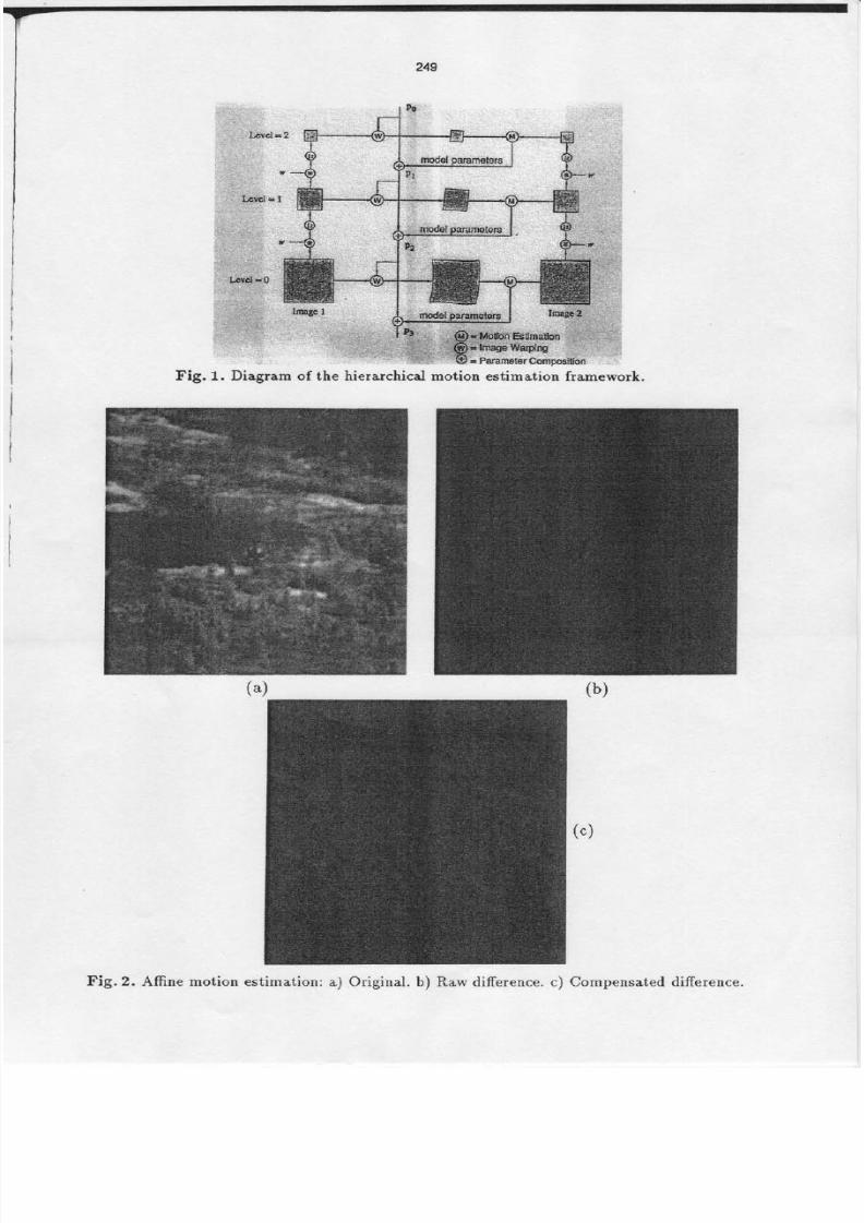
Experiments with the affine motion model: To demonstrate use of the affine flow

model, we show its performanceon an aerial image sequence.A frame of the original

sequence s shown in Figure 2a and the unprocesseddifferencebetween two frames of

this sequences shown in rigure 2b. Figure 2c showsthe result of estimating an affi'ne

transformation usingthe hierarchicalwarpmotion approach,and then usingthis to com-

pensate for cameramotion induced flow. Although the terrain is not perfectly flat, we

still obtain encouragingcompensation esults. In this examplethe simple difierencebe-

tween the comp"orJt"J and original image s sufficient to detect and locate a helicopter

in the image.We use extensionsof the approach, ike integration of compensateddiffer-

ence magesover time, to detect smallerobjects moving more slowly with respectto the

background.

3.2 Planar Surface Flow

The Model: It is generallyknown that the instantaneousmotion of a planar surface

undergoingrigid *otion can be describedas a secondorder function of imagecoordinates

involving eight independentparameters e.g.,see 15]): n this sectionwe providea brief

derivation of this descriptiona,ndmakesomeobservationsconcerning ts estimation'

We begin by observing hat the imagemotion inducedby " rigidly moving object (in

this casea plane)' can be written as:

u(x)fuo(*)t*B(x)c.r

whereZ(*)is the distance rom the cameraof the point (i.e.,depth) whose mageposition

is(x)' and

A(*) = [-J o"lL o -f aJ

(8)

B(x) =

The A and the B matrices dependonly on the image positions and the focal length f

and not on the unknowns:t, tle translation vector, c, the angular velocity vector, and

Z .

A planar surfacecan be describedby the equation

k t X * k z Y * k s Z = l

to the surfaceslant, tilt, and the distance of the plane from

coordinate system (in this case,the camera origin). Dividing

| @il/f -(f + *\lf v ILtr+ f) lr -@v)lr -x) '

(e)

where (kt,kr,lca) relate

the origin of the chose

throughout by Z, we get

t =k++k,I*kg.

using k to denote he vector tc1kz,ks) and r to denote he vector(*lf ,vlf ,1 ) we obtain

z(*)

Substituting this into Equation 8 gives

- r(x)"k.

(10)u(x) = (A(x)t) (r(x)"k) + B(x)r.r



f

243

This flow field is quadratic in (x) and can be written also as

u(x) - a1* a2x* aey azxz asxy

o(x) - &4* asc* aaU azxU aeUz (11 )

where he 8 coefficients41,...,og) are functionsof the motion paramters ,cl and thesurfaceparmetersk. Since his 8-parameter orm is rather well-known (e.g.,see [15])we

omit its details.

If the egomotionparametersare known, hen the three parametervector k can be usedto represent he motion of the pla^nar urface.Otherwisethe 8-parameter representationcan be used. In either case, he flow field is a linear in the unknown pa,rameters.

The problem of estimating pla^nar urfacemotion has been has been extensivelystud-ied before[21,1, 23]. n particular, Negahdaripour nd Horn [21]suggest terative meth-ods for estimating the motion and the surfaceparameters,a"swell as amethod of estimat-ing the 8 parametersand then decomposinghem into the five rigid motion parameters

the three surfaceparameters n closed orm. Besides he embeddingof thesecomputations

within the hierarchicalestimation framework,we also take a slightly different, approachto the problem.

We assume hat the rigid motion parametersare already known or can be estimated(".9., seeSection3.3 below).Then, the problem reduces o that of estimating he threesurfaceparametersk. There are severalpractical reasons o prefer this approach:First, inmany situations the rigid motion model may be more globally applicable han the planarsurfacemodel, and can be estimated using nformation from all the surfacesundergoingthe samerigid motion. Second,unless he region of interest subtends a significant fieldof view, the second order components of the flow field will be small, and hence theestimationof the eight parameterswill be inaccurateand the processmay be unstable.On the other hand, he informationconcerning he threeparameters is contained n thefirst order componentsof the flow field, and (if the rigid motion parametersare known)their estimation will be more accurateand stable.

The Estirnation Algorithm: Let ki denote the current estimate of the surface pa-rameters,and let t and cudenote the motion parameters.Theseparametersare used toconstruct an initial flow field that is used n the warping step. The residual nformationis then used to determine an incrementalestimate 6k.

By substituting the parametric orm of 6u

6 u = u - u 0

= (A(x)t) (r(x)"(ko + 6k)) * B(x)c., (a(*)t) (r(x)"ko) + B(x)c.,

- (A(x)t) r(x)"6k (12)

in Equation 3, we can obtain the incrementalestimate 6k as the vector that minirnizes:

E(6k) I( @t+ (vD"(n )r"ar)2x

Minimizing this error leads o the equation:

r,[I

"(rtA"Xv/)(v/)'(At)r")] ru = -I "(t'A"Xv/)aI

This equation can be solved o obtain the incemental estimate dk.

(13)

(14)



244

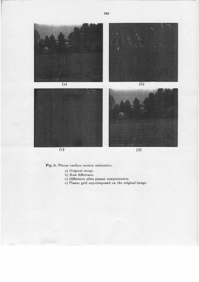
Experiments with the planar surface motion model: We demonstrate he appli-

cation of the planar ,,rrf*" model using images rom an outdoor sequence. ne of the

input images s shown in Figure 3a, u"a trt" differencebetween both input images s

shown in Figure Bb. After esiimating the cameramotion between the imagesusing the

algorithm described n SectionJ.3, i" opplied the plana,rsurfaceestimationalgorithm

to a manually selected magewindow placed roughly over a regionon the ground plane'

Theseparameterswere hen used o warp the second rame towardsthe first (this process

should align the ground plane alone).The difierencebetween his warped imageand the

original image , Jho*r, in rigu. e lc'.The figure showscompensationof the ground plane

motion, leavingresidualpuru,Ilr*motion of tle treesand other objects n the background'

Finally, in order to demonstrate he plane-fit,we graphicallyprojected a rectangulargrid

onto that prane.This is shownsuperimposedon the input image n Figure 3d.

3.3 Rigid BodY Model

The Model: The motion of arbitrary surfacesundergoingrigid mo_tion annot usually

be describedby a singleglobalmodel.We can howevermakeuseof the global rigid bgat

model if we combine t with a local model of the surface. n this section, we provide a

brief derivation of the global and the local models. Hanna [12] providesfurther details

and results, and also dkcribes how the local and global models interact at corner-like

and edge-like magestructures.

As described n Section8.2, the image motion induced by a rigidity moving object

can be written as:

'(x)=fun(*)t*B(x)c.,

(15)

where z(*) is the distance rom the cameraof the point (i.e., its depth), whose mage

position is (x), and

A(*)[-ot,X]

B(x) -

The A and the B matrices dependonly on the imagepositionsand the focal length

f and not on the unknowns: , th; translation vector, c.r he angula,r elocity vector, and

Z . Eqaalion lb relatesthe parametersof the global model, c.rand t, with pa'rametersof

the local scene tructure, Z(x)'

A local model we use s the frontal-planarmodel, which means hat over a local image

patch, we assume hat z(*) is constant.An alternative model uses he assumption hat

bZ 1*1-the differencebetweena previousestimate and a refined estimate-is constant

over each ocal imagePatch.We refinethe local and globalmodels n turn using nitial estimatesof the local struc-

ture parameterc,z(x), and the globat rigid body paiameters @and t. This local/global

refinement is iterated several imes'

The Estimation Algorithm: Let the current estimates be denoted as Z;(Ill.*l :"d

cr.r;. s in the other models,we can use the model parameters o construct an initialflow

field, ,i(*), which is used o warp oneof the imag" fru*"r towardsthe next. The residual

error between the warped image and the originJ imageto which it is warped is used to

| @illf -u2 +,\lf v IL(r'+ v2)lf -@v)lf -x l



245

refine the parametersof the local and globalmodels.We now showhow these modelsarerefined.

We begin by writing equation 15 n an incremental orm so that

du(x) jft.A(x)t*B(x)..,#A(x)ts -B(x)c.,s

Inserting the parametric form of du into Equation 3 we obtain the pixel-wiseerror as

E(t,u,Lf (x))= (at + (vr)"N/z(x) + (v|rBu - (vr)" Ari/zi(x) (v4"B r,)'(17)

To refine he local models,weassumehat L/Z(x) is constantover5 x 5 imagepatchescentered on each image pixel. We then algebraically solve for this Z both in order toestimate its current value, and to eliminate it from the global error measure.Considerthe local component of the error measure,

Eto"ot I E(t ,w, I /Z(x)) .5 x E

Differentiating quation17with respect o I/Z(x) andsetting he result o zero,weget

L/z(x)-- Ibxs(VI)"At (4/ - gz/)rAtilzd(x),+ (V/)"gc.t (v l)r3,w;) t1(

Du*u((vr;r6*' '

' \ ' ' (19)

To refine the global model, we minimize the error in Equation L7 summed over the

entire image:

Estobatt

E(t ,u, I /Z(x)) .

Image

We insert the expression or | / Z (x) given in Equation L9-not the current numeri,cal

aalue of the local parameter-into Equation 20. The result is an expression or Eilobarthat is non-quadratic in t but quadratic in c.r We recoverrefined estimatesof t a,ndc.r

by performing one Gauss-Newtonminimization step using the previousestimatesof theglobal parameters, i and arg,as starting values.Expressionsa,reevaluated numericallya t t ; a n d u ) = u ) i .

We then repeat the estimation algorithm several imes at each mage resolution.

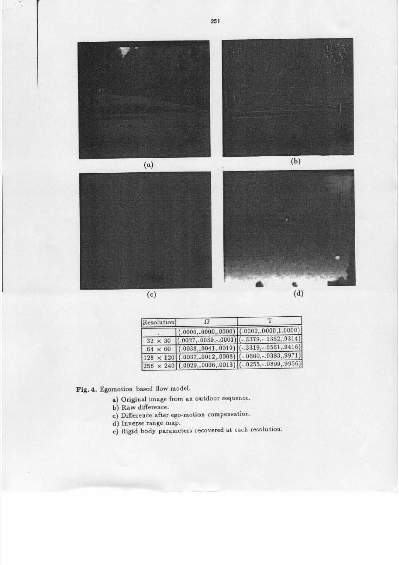
Experiments with the rigid body motion model: We have chosenan outdoor scene

to demonstrate the rigid body motion model. Figure 4a shows one of the input images,

and Figure 4b shows the differencebetween the two input images.The algorithm wasperfiormedbeginning at level

3(subsampledby u factor of

8)of a Laplacianpyramid. The

local surface parametercIf Z(x) were all initialized to zero, and the rigid-body motionparameterswere nitialized o t0 = (0,0, 1)T and u)= (0,0,0)t.The modelparameterswere refined 10 times at each image resolution. Figure 4c shows the difierence image

between he second mage and the first image after being warpedusing he final estimates

of the rigid-body motion parametersand the local surfaceparameters.Figure 4d shows

an image of the recovered ocal surfaceparameterc f Z(x) such that bright points are

nea,rer he camera than dark points. The recovered nverseranges are plausible almost

everywhere,except at the image border and near the recovered ocus of expansion.The

bright dot at the bottom right hand side of the inverse ange map corresponds o a leaf

in the original image that is blowing acoss the ground towa"rds he camera.Figure 4e

(16)

(18)

(20)



246

shows a table of rigid-body motion parameters that were recovered at the end of each

resolution of analysis.

More experimental results and a detailed discussion of the algorithm's performance

on va.rious types of scenes can be found in [12].

3.4 General Flow Fields

The Modeh Unconstrainedgeneral low fields are typically not describedby any globalparametric model. Different local modelshavebeen used to facilitate the estimation pro-

cess,ncluding constant low within a local window and locally smoothor continuous low.

The former facilitates direct local estimation [18,20], whereas he latter model requires

iterative relaxation techniques 16] tt is also not uncommon to use the combination of

these wo types of local models ".g., [3, 10]).The local model chosenhere s constant flow within 5 x 5 pixel windows at each evel

of the pyramid. This is the sarnemodel as used by Lucas and Kanade [18]but here it is

embeddedas a local model within the hiera,rchicalestimation framework.

The Estirnation Algorithm: Assume that we have an approximate flow field fromprevious evels (or previous terations at the same evel). Assuming that the incremental

flow vector 6u is constant within the 5 x 5 window, Equation 3 can be written as

E(6u) f{a I +vfr6') 'x

where the sum is taken within the 5 x 5 window. Minimizing this error with respect o

6u leads o the equation,

[Itotxvo'] 6u--I vIAI. (22)

(2r)

We make some observationsconcerning he singularities of this relationship. If the sum-*ittg window consists of a singleelement, the 2 x 2 matrix on the left-hand-side s anouter product of a 2 x I vector and hence has a rank of atmost unity. In our case,whenthe sum*ittg window consistsof 25 points, the rank of the matrix on the left-hand-sidewill be two unless he directionsof the gradientvectorsV.I everywherewithin the windowcoincide.This situation is the generalcaseof the aperlure effect.

In our implementation of this technique, he flow estimate at eachpoint is obtainedbyusing a 5 x 5 windows centeredaround that point. This amounts to assuming mplicitly

that the flow field variessmoothly over the image.

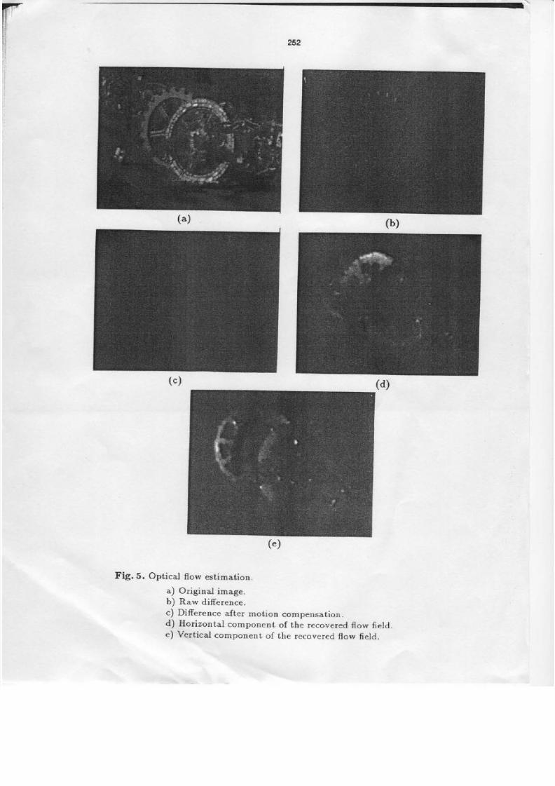
Experiments with the general flow model: We demonstrate he general low algo-rithm on an image sequence ontaining several ndependently moving objects, a case orwhich the other motion models describedhere are not applicable. Figure 5a shows one

image of the original sequence.Figure 5b showsthe difference between the two framesthat wereused o compute mage low. Figure 5c shows ittle differencebetween he com-pensated mage and the other original image. Figure 5d shows he horizontal componentof the computed flow field, and figure 5e shows he vertical component. In local imageregionswhere image structure is well-defined,and where the local image motion is sim-

ple, the recoveredmotion estimates appear plausible. Errors predictably occur howeverat motion bounda^ries. rrors alsooccur in image regionswherethe local image structure

is not well-defined like someparts of the road), but for the same rea"son, ucherrors do

not appear as ntensity errors in the compensateddifference mage.



247

4 Discussron

Thus far, we havedescribeda hierarchical ramework for the estimation of imagemotionbetweentwo imagesusing va^riousmodels.Our motivation was to generalize le notionof direct estimation to

model-basedestimation and unify a diverseset of model-basedestimation algorithms nto a single ramework.The frameworkalsosupportsthe combineduse of parametric globalmodels and local models which typically representsometype ofa smoothnessor local uniformity assumption.

One of the unifying aspectsof the framework is that the same objective function(SSD) is usedfor all models,but the minimization is performedwith respect to differentparameters.As noted in the introduction, this is enabledby viewingall theseproblemsfrom the perspectiveof image registration.

It is interesting to contrast this perspective(of model-based mageregistration) withsome of the more traditional approaches o motion analysis.One such approach is tocompute image low fields, which involvescombining the local brightness constraint withsomesort of a global smoothnessa^ssumption,nd then interpret them usingappropriatemotion models.In contrast, the approach aken here is to use the motion models toconstrain the flow field computation. The obvious benefit of this is that the resultingflow fields may generallybe expected to be more consistent with models than generalsmooth flow fields.Note, however, hat the frameworkalso ncludesgeneral *ooih flowfield techniques,which can be used f the motion model s unkno*n.

In the caseof models hat are not fully parametric, ocal image nformation is usedtodetermine ocal image/scene roperties(e.g., he local rangevalue).However, he accu-racy of thesecan only be as good as the available ocal image nformation. For example,in homogeneous reasof the scene, t may be possible o achieveperfect registration even

if the surfacerange estimates (and the corresponding ocal flow vectorsf are incorrect.However, n the presenceof significant image structures, these local estimates may beexpected o be accurate.On the other hand, the accuracyof the globalparameters e.g.,the rigid motion parameters) dependsonly on having sufficient and sufficiently diverselocal information across he entire region.Hence, t may be possible o obtain reliableestimatesof theseglobal parameters,even though estimated local inf,ormationmay notbe reliable everywherewithin the region.For fully parametric models, his problem doesnot exist.

The image registration problem addressedn this paper occurs in a wide range ofimage processingapplications, far beyond the usual ones considered n computer vision(".9., navigationand imageunderstanding).These nclude magecompression ia

motioncompensatedencoding,spatiotemporal analysisof remote sensing ype of images, magedatabase ndexing and retrieval, and possibly object recognition. On" way to state thisgeneralproblem is as that of recovering he coordinatesystem that relate two imagesofa scene aken from two different viewpoints. In this sense, he framework proporuJ h"r"unifiesmotion analysisacross hesediferent applicationsas well.

Acknowledgements: M*y individuals havecontributed to the ideas and results pre-sentedhere.These nclude Peter Burt and LeonidOliker from the David SarnoffResearchCenter, and ShmuelPeleg rom HebrewUniversity.



248

References

1. G. Adiv. Determining three-dimensionalmotion and structure from optical flow generated

by severarmoving objects IEEE Trans. on pattern Anorysis and Machine Intelligence,

2 .

3 .

4.

?( ):384-401,JulY1985-

p. Anandan. A unified perspectiveon computational techniques or the measurementof

visual motion. rn Internationarconferenceon computer vision, pages zl9-230, London,

May 1987.p. Anandan. A computational framework and an algorithm for the measurementof visual

motion. International Journalo! computer vision,2z283-3L0, 1989'

J. R. Bergen and E. H. Adersoo. Hi.rarchicar, computationaly efrcient motion estimation

algori thm.J. Opt. Soc.Am' A',4:35,1987'

s. lt;:';;;, ;1. ir"rr,'ii. Hinsorani,lnds. pereg.computing wo motions rom three

- l - - T^ -^ - T \^^o - l ' o . 1 OOf)

;;;;"ii"i)rr)r""t;;;' c;;i;"ce on computer vision,osaka,Japan,December ee0'_ - . r ^ T t r 1 Efall les. lll rt

6. p. J. Burt and E. H. Adelson. The raprr.ino pyramid as a compact image code. IEEE

Transactions n c ommunication, 1:532-540,1983.

Tt 5,ol'

/d!a e

Awl;. #""rrJ;."b;;:;-;;;;kfi.,oi*, a movingcamera,an apprication f dvnamicmotion

. f 1 t A l f , ^ - ^ L' l

oQ o

;;il: i"'ioii i";i;;;o\n visuarMotion,ases -12, r-vine,A, March1e8e-- - : - ^ l ^ 1 i - - ^ ^ r n h a n a n

LItCLIJDrD. - r r1

g. p.J. Burt, R. llingorani, and R. J. Kolczynski. Mechanisms for isolating component pat-I r : ^ ^ . - l i f ^+ : ^ ^

terns in the sequential analysisof multipre motion. rn IEEE workshop on visual Motion,

pages187-193,Princeton,NJ , October1991'

g. stefan carlsson. object detection using model basedprediction and motion parallax' In

stockholmworkshop n computationaluision,stockholm, sweden,August 1989'

J. Dengler. Locar motion estimationwith the dynamic pyramid. rn Pgrarnidal ystemsor

,o*pul", aision,pages 89-298,Maratea, Italy' May 1986'

w. Enkelmann. Investigationsof multigrid algorithmsfor estimation of optical flow fields n

imagesequences.ComJuter Vision, Giaphics,and mageProcessing 339:150-L77'1988'

K. J. Hanna. Direct multi-resolution estimation of ego-motion and structure from motion'

ln Workshopon Visual Motion'pages156-162,Princeton, NJ, October 1991'| . ,Tt^^l

13. :: ri:"i5't;:;':rir**i.";il;;;e and *oiioo rrommultiple rames'TechnicalReport

1190,MIT AI LAB, Cambridge,MA, 1990'

E. C. Hildreth The Messureme,nt! visual Motion' The MIT Press'1983'

B .K.P. I l o rn .RobotV is ion , .MITPress ,Cambr idge,MA,1986.

B. K. p. Horn and B. G. Schunck.Determiningoptical flow. Artificial Inteuigence,r7:L85-

203,1981.

17. B. K. p. Horn and E. J. weldon. Direct methods for recoveringmotion. International

Journal f ComputerVision,2(1):51-76'June 1988'

1g. B.D. Lucasand T. Kanade.'Ao

'it"r.tiveimage registration echniquewith an application

to stereovision. In Image JnderstsndingWorkshop' ages121-130,1-991'

l: il=jfit;'*. s;"ilil:;;J i: K;";J;. Karman'ftt"'-u.'ed lgorithmsorestimatingr l f :9. L. Matthtes, K. SzensKl' ar

depth from image-sequences. rn International conference on computer vision, pages 199-

213,TamPa,FL, 1988'

zo. H. H. Nagel. Displacementvectors derived from secondorder intensity variations in in-

tensity sequences. computer vision, Pattern reognition and mage Ptocessing,2T:85-ll7

1983.

zr. s. Negahdaripour and B.K.p. Ilorn. Direct passivenavigation. IEEE Trans. on Pattern

Analysisand Machine ntelligence, (1):168-1?6,January 1987'

22. A. Singh. An estimation theoretic framework for image-flowcomputation. ln International

Confeience n Computer Vision,Osaka,Japan' November1990'

;:#:ffiff;;;?:w;;:'b;;;;;; ""i"ii.n, neighborhooderormationndgrobar. - L , / e \ . o <

image flow: planar surfaces in motion . International Joirnal of RoboticsReseotch,4(3):95-

10.

1 1 .

12.

14.

15 .

16 .

23.

108,Fall 1985.



Fig. 1. framework.iagram of the hierarchical motion estimation

Fig.2. Affine motion estimation: a) Original. b) Raw difference. c) Compensated difference.



Fig.3. Planar surface motion estimation.

a) Original image.

b) Raw diference.

.) Diff"r"nce after planar compensation.c) Planar grid superimposed on the original image.



&(a)

(.oooo,.ooo0,.oooo).0000, .0000,1.0000)

3 2 x 3 0 .0027,.0039,-.0001-.3379,- .152, .9314)

6 4 x 6 0 (.0038, .0041, .0019-.33 9,- .0561, .94)

128 x 120 (.003?, .0012, .0008).oooo,-.0383,.9971)

256 x 240 (.oozg,.oo06,.oo13).0255,- .0899, .9956)

Fig.4. Egomotion based flow model'

a) Original image from an outdoor sequence'

b) Raw difference.

c) Difference after ego-motion compensation'

d) Inverse range map.

"j nigia body parameters recovered at each resolution.



252

(d)

(" ) (b)

(")

(" )

Fig.5. Optical f low estimation.

a) Original image.

b) Raw diference.

c) Difference after motion compensation.d) Horizontal component of th e recovered lo w fielcl.

e) Vertical component of the recovered florv field.

Documents

01.13.Hierarchical Model-based Motion Estimation