MOTION CONTROLAPPLICATION NOTES

BALDOR ELECTRIC COMPANY

MN1200

Page 1

Application Notes

TABLE OF CONTENTS

BASICS OF MOTION . . . . . . . . . . . . . 13

CONVERSION TABLES. . . . . . . . . . . 26

DRIVE TECHNOLOGY . . . . . . . . . . . 1

INERTIA MATCHING . . . . . . . . . . . . 22

IS IT DC OR AC BRUSHLESS?. . . . . 17

MATCHED PERFORMANCE . . . . . . 11

MECHANICS . . . . . . . . . . . . . . . . . . . . 7

Page 2

Application Notes

Page 3

Application Notes

Drive Technology

The following explores the world of drives, and explainswhere each is best used.

There are inverter, vector, servo, and now linear drive technologies available. What type of technol-ogy should be considered depends upon the application needs.

Inverter Drives

Inverter techniques are used to control an induction motor. These use either six-step techniques orsynthesize a sinusoidal waveform. The frequency of the generated waveform controls motor speed.

This control, with a standard AC induction motor, would provide a speed regulation (limited tothe slip of the motor) of approximately 1.5-3 percent of base speed. The low-end controllable speedwill start about 300 rpm. From there, constant torque can be provided to base speed with constanthorsepower to 1.5 times base speed.

Some advantages of inverter drives include low initial cost due to simplicity of motor design, relia-bility, and ease of use. Design specifications include peak overload capacity of 150-200%, controlledreversing, pre-set speeds, and programmable I/O’s to mention a few.

This technology works well for many adjustable-speed applications, such as centrifugal fans,conveyors, pumps, mixers, and packaging equipment.

Vector Drives

Vector control technology primarily uses a PWM synthesized sinusoidal waveform to controlmotor speed. An induction motor can be controlled by vector control technology. The only require-ment is that an appropriate feedback device, such as an encoder, be used.

These controls can provide tighter speed regulation approaching 0.01 percent of set speed.Controllable speed ranges from zero speed to about 5 times base speed are attainable. The constanthorsepower range will be about 3.5 times the base speed.

In order to provide the most reliable and efficient package for the application, the vector motorshould be designed with a high-efficient winding, an efficient lamination design, and high-temper-ature insulation materials. The electrical winding must be protected against high dv/dt rates (shortrise time pulses) and voltage reflections which will degrade the electrical winding life. Spike resis-tant wire has been designed for motors controlled by inverters and vectors. The additional protec-tion , which this wire provides, results in longer motor life, reduced down time, and better overallvalue. All Baldor motors include the above features, designed in as standard.

If the application has high inertial loads, a line regeneration (“line regen”) vector control should beconsidered. “Line regen” controls save energy by returning the energy (power generated by themotor) back to the incoming power line. Additionally, since these designs operate near unitypower factor, they result in additional energy savings.

Advantages of vector drive technology includes low initial cost, reliability, capability of ratedtorque to zero speed, precise speed control, long life, constant horsepower output above ratedspeed, and such programmable features as controlling acceleration/deceleration time, and tuningof the control.

Page 4

Application Notes

Vector drives are used in high-performance adjustable-speed applications, machine tool spindles,and industrial test stands just to mention a few applications. Line regen units are used in winders,hoist/crane, presses, HVAC, and other applications. For positioning applications, vector drives areused with existing programmable position controllers.

DC Servo Drives

In the world of servos, there are DC servos and brushless servos. The brushless servos are termed,by manufacturers, as either DC or AC.

The DC servo package takes AC power in, and converts it to DC. The amount of DC output appliedto the motor is directly proportional to the desired operating motor speed. The performanceprovided by DC servos may be considered as “traditional”, and comparable to vector technologywhen used with a positioning package.

Advantages of DC servos include proven reliability and well known technology (they have beenaround forever). In positioning applications, and in comparison to vectors, DC servos come in asmaller package size and provide lower inertia, which translates to faster acceleration (gets intoposition faster). When used within the designed capability range, the DC servo motor, with itsbrush design, provides a long adequate life for many applications.

DC servos are used in machine tool, factory automation, packaging, woodworking, and manyother applications.

Brushless Servo Drives

As indicated, brushless servos are available as either DC brushless or AC brushless. The feedbackdevice determines whether it is considered DC or AC, since this dictates the control scheme. Thefeedback device may be either Hall sensors, encoders, or resolvers.

With Hall sensor feedback, the three-phase brushless motor is powered by energizing two of thethree motor windings at a time. There are six different commutation sections for one mechanicalrevolution, and within each commutation section, a DC level of power is applied. The amount ofDC applied is directly proportional to the desired operating motor speed. Thus the term “DCbrushless”.

Encoder feedback is used when position data is required in the application. Some encoders areavailable with Hall outputs. Again, the Hall signals are used for commutation of the brushlessmotor.

With resolver feedback, a sinusoidal waveform is applied on the motor windings. Thus the term“AC brushless”. The advantage of this technology is that, for the same torque (compared to “DCbrushless”), the “AC brushless” will require less current. Therefore a smaller drive may often beused in the application. This becomes possible since the motor has a three phase sinusoidalwinding being powered by a three phase sinusoidal current waveform.

Advantages of brushless technology include higher speed capability, higher torques in a smallerpackage, much lower inertia (thus much faster acceleration capability), and of course, long reliablemaintenance free life in the application. These drives provide good low speed operation down tozero speed. Brushless controls are available with auto-tuning capability.

Brushless drives are used in robotics, packaging, electronic assembly, semiconductor equipment,textile, and any cutting, printing or labeling which may even be performed on a moving web.Many other applications of course exist.

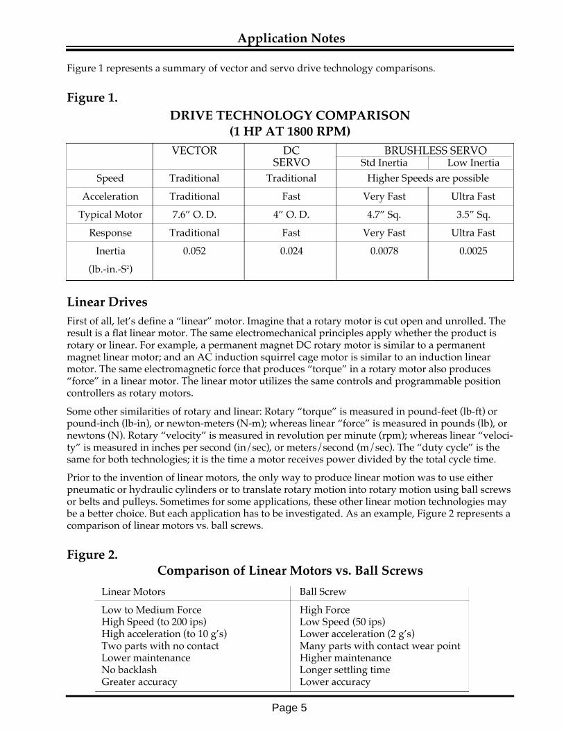
Figure 1 represents a summary of vector and servo drive technology comparisons.

Figure 1.

Linear Drives

First of all, let’s define a “linear” motor. Imagine that a rotary motor is cut open and unrolled. Theresult is a flat linear motor. The same electromechanical principles apply whether the product isrotary or linear. For example, a permanent magnet DC rotary motor is similar to a permanentmagnet linear motor; and an AC induction squirrel cage motor is similar to an induction linearmotor. The same electromagnetic force that produces “torque” in a rotary motor also produces“force” in a linear motor. The linear motor utilizes the same controls and programmable positioncontrollers as rotary motors.

Some other similarities of rotary and linear: Rotary “torque” is measured in pound-feet (lb-ft) orpound-inch (lb-in), or newton-meters (N-m); whereas linear “force” is measured in pounds (lb), ornewtons (N). Rotary “velocity” is measured in revolution per minute (rpm); whereas linear “veloci-ty” is measured in inches per second (in/sec), or meters/second (m/sec). The “duty cycle” is thesame for both technologies; it is the time a motor receives power divided by the total cycle time.

Prior to the invention of linear motors, the only way to produce linear motion was to use eitherpneumatic or hydraulic cylinders or to translate rotary motion into rotary motion using ball screwsor belts and pulleys. Sometimes for some applications, these other linear motion technologies maybe a better choice. But each application has to be investigated. As an example, Figure 2 represents acomparison of linear motors vs. ball screws.

Figure 2.Comparison of Linear Motors vs. Ball Screws

Page 5

Application Notes

DRIVE TECHNOLOGY COMPARISON(1 HP AT 1800 RPM)

VECTOR DC BRUSHLESS SERVOSERVO Std Inertia Low Inertia

Speed Traditional Traditional Higher Speeds are possible

Acceleration Traditional Fast Very Fast Ultra Fast

Typical Motor 7.6” O. D. 4” O. D. 4.7” Sq. 3.5” Sq.

Response Traditional Fast Very Fast Ultra Fast

Inertia 0.052 0.024 0.0078 0.0025

(lb.-in.-S2)

Linear Motors Ball Screw

Low to Medium Force High ForceHigh Speed (to 200 ips) Low Speed (50 ips)High acceleration (to 10 g’s) Lower acceleration (2 g’s)Two parts with no contact Many parts with contact wear pointLower maintenance Higher maintenanceNo backlash Longer settling timeGreater accuracy Lower accuracy

Page 6

Application Notes

Advantages of linear motors include high acceleration (up to 10 g’s), low speed (0.0001inch/second) and high speed (100 inch/second) capability, small strokes (0.01 inch) and longstrokes (excess of 25 feet), and sub-micron position accuracy (with appropriate feedback device).Only one moving part leads to simplicity and high reliability, with no backlash and very high stiff-ness. The non-contact parts reduce wear leading to long life and reduction in maintenance.

Linear drives are used in semiconductor, material handling, robotics, medical, people movers, andpackaging just to indicate a few applications.

Conclusion

For proper sizing and selection, an applications’ speed (and speed range), inertia (and inertiamatching) and acceleration (relates to overload or peak capacity), and package size (relates tosmaller, lighter motor in some technologies), all should be reviewed.

Page 7

Application Notes

Mechanics

This application note presents formulas for calculatingreflected load parameters.

The mechanical systems used in motion control applications can be divided into four basiccategories: direct, gear, belt-pulley and leadscrew. Reflecting parameters back to the motor shafteases the calculations necessary for sizing and selecting.

Cylinder Inertia

The first formula is for calculating the inertia of a cylinder. This is important since many mechani-cal components can be calculated using this formula.

The inertia of a solid cylinder can be calculated if either the weight and radius, or the density andradius and length are known.

The inertia of a hollow cylinder can be calculated if the weight and radius are known, or the densi-ty and radius and length are known.

For known weight and radius: JL = 1 W r2

2 g

For known density, radius and length: JL = 1 πlpr4

2 g

Where: JL = inertia (lb-in-s2)W = weight (lb)r = radius (in)l = length (in)p = density of material (lb/in3)g = gravitational constant (386 in/s2)

For known weight and radius: JL = 1 W (ro2 + ri

2)2 g

For known density, radius and length: JL = π lp (ro4 - ri

4)2 g

Where: JL = inertia (lb-in-s2)W = weight (lb)ro = outside radius (in)ri = inside radius (in)l = length (in)p = density of material (lb/in3)g = gravitational constant (386 in/s2)

Page 8

Application Notes

The inertia of complex concentric rotating parts is calculated by breaking the part up into simplerotating cylinders, calculating their individual inertia, and adding them together.

Direct Drive

For direct drive loads, there are no mechanical linkages.

Speed: WM = WL

Inertia: JT = JL + JM

Torque: TL = T’

Where: WM = motor speed (rpm)WL = load speed (rpm)JT = total system inertia (lb-in-s2)JL = load inertia (lb-in-s2)JM = motor inertia (lb-in-s2)TL = load torque at motor shaft (lb-in)T’ = load torque (lb-in)

J = J1 + J2 + J3

Total

Material Densities

Material lb/in3

Aluminum 0.096Brass 0.300Bronze 0.295Copper 0.322Steel (cold rolled) 0.280Plastic 0.040

Page 9

Application Notes

Gear

Loads in a gear application have to be reflected back to the motor shaft by the gear ratio, or the gearratio squared. The inertia of the gears have to be included in the calculations. Gear inertia may becalculated using the formula for cylinder.

Belt and Pulley

The load parameters have to be reflected back to the motor shaft. Although a belt and pulleyarrangement is shown, it can also be a rack and pinion, or timing belt and pulley, or chain andsprocket. The inertia of the pulleys, sprockets, or pinions must be included.

Speed: WM = WL (NL/NM)

Inertia: JT = (NM/NL)2 (JL + JNL) + JM + JNM

Torque: TL = T’ (NM/NL)

Where: WM = motor speed (rpm)WL = load speed (rpm)NM = number of motor gear teethNL = number of load gear teethTL = load torque at motor shaft (lb-in)T’ = load torque (lb-in) - not reflectedJT = total system inertia (lb-in-s2)JL = load inertia (lb-in-s2)JM = motor inertia (lb-in-s2)JNM = motor gear inertia (lb-in-s2)JNL = load gear inertia (lb-in-s2)

Speed: WM = 1 VL

2π r

Inertia: JT = W r2 + JP1 + JP2 + JM

g

Torque: TL = FFr + FLr

Where: WM = motor speed (rpm)VL = linear load speed (inch/min)r = pulley radius (in)TL = load torque reflected to motor shaft (lb-in)TF = friction torque (lb-in)FL = load force (lb)JT = total system inertia (lb-in-s2)JM = motor inertia (lb-in-s2)JP = pulley inertia (lb-in-s2)W = load weight including belt (lb)FF = frictional force (lb)g = gravitational constant (386 in/s2)

Page 10

Application Notes

Leadscrew

The load has to be reflected back to the motor shaft. The leadscrew inertia has to be included (canuse the formula for inertia of a cylinder). If preloading is used the torque must be included since itmay be significant.

Speed: WM = VLP

LoadTorques: TL = 1 FL + 1 FPF x 0.2

2π pe 2π p

Friction TF = 1 µW cos o + W sin oTorques: 2π pe

Inertia: JT = W ( 1 )2 1 + JLS + JM

g 2πp e

Where: WM = motor speed (rpm)VL = linear load speed (in/min)p = lead screw pitch (revs/in)e = lead screw efficiencyTL = load torque at motor shaft (lb-in)TF = friction torque (lb-in)FL = load force (lb)FPF = preload force (lb)JT = total system inertia (lb-in-s2)JM = motor inertia (lb-in-s2)JLS = lead screw inertia (lb-in-s2)W = load weight (lb)FF = frictional force (lb)µ = coefficient of frictiong = gravitational constant (386 in/s2)

Typical Efficiencies

Type Efficiency

Ball-nut 0.90

Acme with plastic nut 0.65

Acme with metal nut 0.40

Coefficient of Friction

Material Coefficient

Steel on steel 0.580

Steel on steel (lubricated 0.150

Teflon on steel 0.040

Ball bushing 0.003

Page 11

Application Notes

Matched PerformanceTM

The information in this application note explains how toread the speed-torque curves.

Baldor provides “matched performanceTM”curves to simplify the process of selecting both a motorand control for a specific application.

Curves

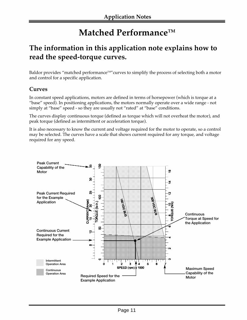
In constant speed applications, motors are defined in terms of horsepower (which is torque at a“base” speed). In positioning applications, the motors normally operate over a wide range - notsimply at “base” speed - so they are usually not “rated” at “base” conditions.

The curves display continuous torque (defined as torque which will not overheat the motor), andpeak torque (defined as intermittent or acceleration torque).

It is also necessary to know the current and voltage required for the motor to operate, so a controlmay be selected. The curves have a scale that shows current required for any torque, and voltagerequired for any speed.

Peak CurrentCapability of theMotor

Peak Current Requiredfor the ExampleApplication

Continuous CurrentRequired for theExample Application

Continuous Operation Area

Continuous Torque at Speed forthe Application

Maximum SpeedCapability of theMotorRequired Speed for the

Example Application

Intermittent Operation Area

Page 12

Application Notes

Example

An application requires a continuous torque of 30 lb-in at a speed of 3750 RPM. The peak torquerequired for acceleration is 80 lb-in.

The curve shows a motor which will work in this application. The bus voltage required is 300 VDC.The continuous and peak currents required are 7 and 18 amps.

A control is selected which can deliver this amount of current or more. The literature wouldindicate the closest control would deliver 10 amps continuous and 20 amps peak with a 230 VACinput (300 VDC bus).

Data Tables

The motor’s voltage constant (back-emf) and torque constant are “cold” values (25°C); the continu-ous stall torque and current are “hot” values (155°C). The temperature coefficient factor between“cold” and “hot” is 0.95 for rare earth motors, and 0.85 for ferrite.

The following will show you how to easily determine theright motor and control for any electromechanicalpositioning application.

Once the mechanics of the appli-cation have been analyzed, andthe friction and inertia of theload are known, the next step isto determine the torque levelsrequired. Then, a motor can beselected to deliver the torqueand the control sized to powerthe motor. If friction and inertiaare not properly determined, themotion system will either taketoo long to position the load, itwill burn out, or it will be unnec-essarily costly.

Motion Control

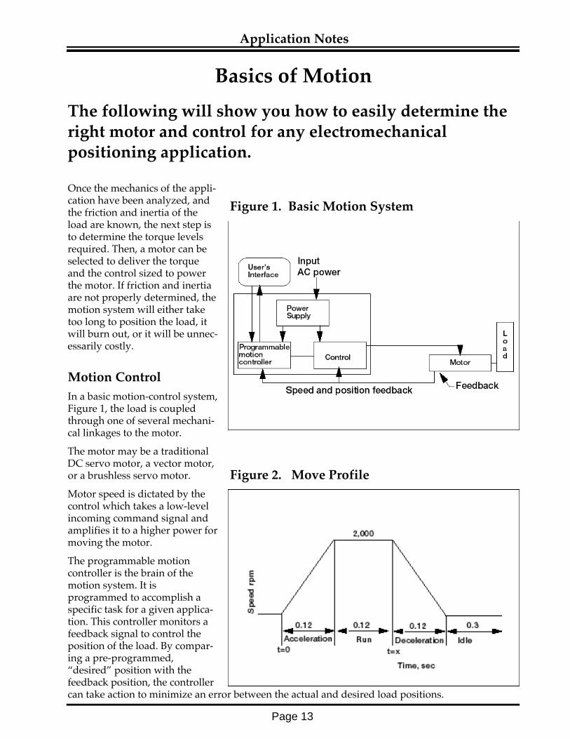
In a basic motion-control system,Figure 1, the load is coupledthrough one of several mechani-cal linkages to the motor.

The motor may be a traditionalDC servo motor, a vector motor,or a brushless servo motor.

Motor speed is dictated by thecontrol which takes a low-levelincoming command signal andamplifies it to a higher power formoving the motor.

The programmable motioncontroller is the brain of themotion system. It isprogrammed to accomplish aspecific task for a given applica-tion. This controller monitors afeedback signal to control theposition of the load. By compar-ing a pre-programmed,“desired” position with thefeedback position, the controllercan take action to minimize an error between the actual and desired load positions.

Page 13

Application Notes

Basics of Motion

Figure 1. Basic Motion System

Figure 2. Move Profile

Movement Profile

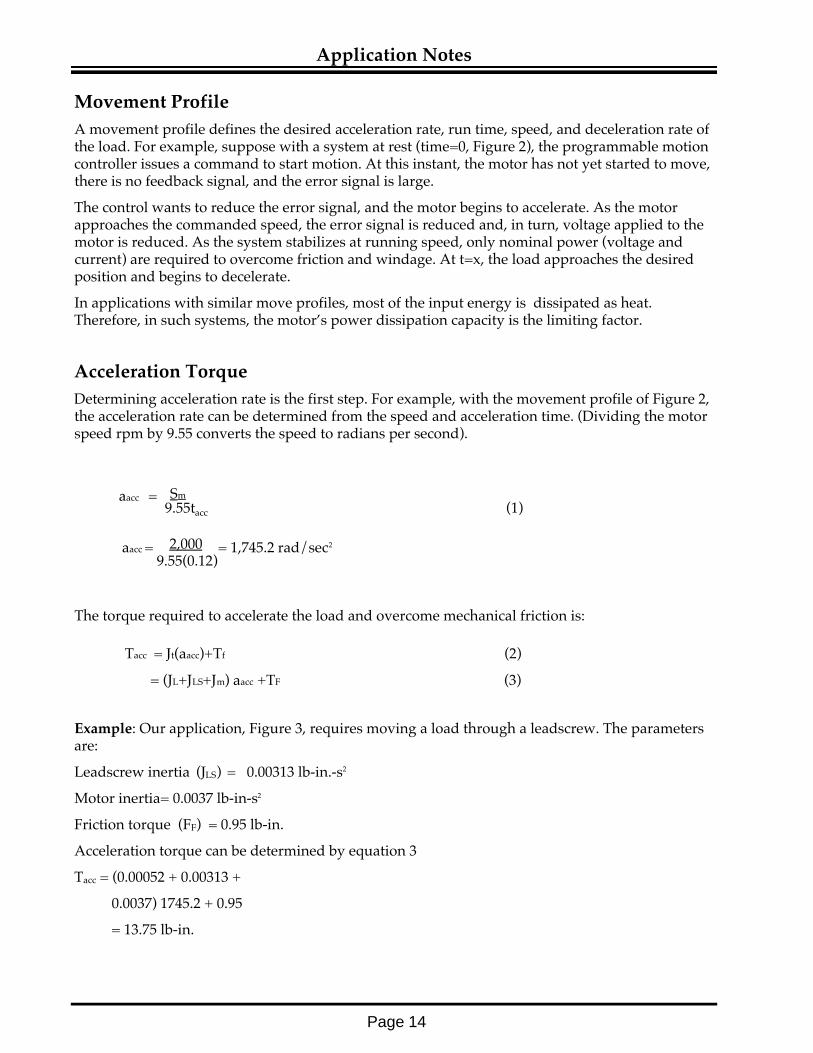
A movement profile defines the desired acceleration rate, run time, speed, and deceleration rate ofthe load. For example, suppose with a system at rest (time=0, Figure 2), the programmable motioncontroller issues a command to start motion. At this instant, the motor has not yet started to move,there is no feedback signal, and the error signal is large.

The control wants to reduce the error signal, and the motor begins to accelerate. As the motorapproaches the commanded speed, the error signal is reduced and, in turn, voltage applied to themotor is reduced. As the system stabilizes at running speed, only nominal power (voltage andcurrent) are required to overcome friction and windage. At t=x, the load approaches the desiredposition and begins to decelerate.

In applications with similar move profiles, most of the input energy is dissipated as heat.Therefore, in such systems, the motor’s power dissipation capacity is the limiting factor.

Acceleration Torque

Determining acceleration rate is the first step. For example, with the movement profile of Figure 2,the acceleration rate can be determined from the speed and acceleration time. (Dividing the motorspeed rpm by 9.55 converts the speed to radians per second).

The torque required to accelerate the load and overcome mechanical friction is:

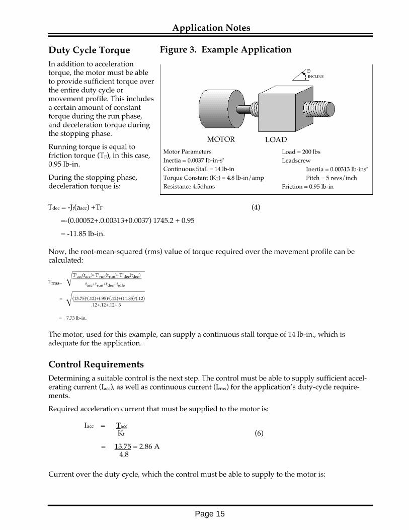
Example: Our application, Figure 3, requires moving a load through a leadscrew. The parametersare:

Leadscrew inertia (JLS) = 0.00313 lb-in.-s2

Motor inertia= 0.0037 lb-in-s2

Friction torque (FF) = 0.95 lb-in.

Acceleration torque can be determined by equation 3

Tacc = (0.00052 + 0.00313 +

0.0037) 1745.2 + 0.95

= 13.75 lb-in.

Page 14

Application Notes

2,000aacc = 9.55(0.12)

= 1,745.2 rad/sec2

Tacc = Jt(aacc)+Tf (2)

= (JL+JLS+Jm) aacc +TF (3)

Smaacc = 9.55tacc (1)

Duty Cycle Torque

In addition to accelerationtorque, the motor must be ableto provide sufficient torque overthe entire duty cycle ormovement profile. This includesa certain amount of constanttorque during the run phase,and deceleration torque duringthe stopping phase.

Running torque is equal tofriction torque (TF), in this case,0.95 lb-in.

During the stopping phase,deceleration torque is:

Now, the root-mean-squared (rms) value of torque required over the movement profile can becalculated:

The motor, used for this example, can supply a continuous stall torque of 14 lb-in., which isadequate for the application.

Control Requirements

Determining a suitable control is the next step. The control must be able to supply sufficient accel-erating current (Iacc), as well as continuous current (Irms) for the application’s duty-cycle require-ments.

Required acceleration current that must be supplied to the motor is:

Current over the duty cycle, which the control must be able to supply to the motor is:

Tdec = -Jt(aacc) +TF (4)

=-(0.00052+.0.00313+0.0037) 1745.2 + 0.95

= -11.85 lb-in.

Page 15

Application Notes

Iacc = Tacc

Kt (6)

= 13.75 = 2.86 A 4.8

Figure 3. Example Application

Trms=

T2acc(tacc)+T2

run(trun)+T2dec(tdec)

tacc+trun+tdec+tidle

= (13.75)2(.12)+(.95)2(.12)+(11.85)2(.12).12+.12+.12+.3

= 7.73 lb-in.

ÎãããããããããÎããããããããã

Motor Parameters

Inertia = 0.0037 lb-in-s2

Continuous Stall = 14 lb-in

Torque Constant (KT) = 4.8 lb-in/amp

Resistance 4.5ohms

Load = 200 lbs

Leadscrew

Inertia = 0.00313 lb-ins2

Pitch = 5 revs/inch

Friction = 0.95 lb-in

Page 16

Application Notes

Power RequirementsThe control must supply sufficient power for both the acceleration portion of the movement profile,as well as for the duty-cycle requirements. The two aspects of power requirements include (1)power to move the load, Pdel, and (2) power losses dissipated in the motor, Pdiss.

Power delivered to move the load is:

Power dissipated in the motor is a function of the motor current. Thus, during acceleration, thevalue depends on the acceleration current (Iacc); and while running, it is a function of the rmscurrent (Irms). Therefore, the appropriate value is used for “I” in the following equation.

Pdiss = I2 (Rm) (9)

The sum of these Pdel and Pdiss determine total power requirements.

Example: Power required during the acceleration portion of the movement profile can be obtainedby substituting in equations 8 and 9:

Note: the factor of 1.5 in the Pdiss calculation is a factor used to make the motor’s winding resistance“hot”. This is assuming the winding is at 155° C.

Continuous power required for the duty cycle is:

In Summary

The control selected must be capable of delivering an acceleration current of 2.86 A, and a continu-ous current of 1.61 A. The power requirement calls for peak power of 380.7 W and continuouspower of 200.4 W.

To aid in selecting, computer software programs are available to perform the iterative calculationsnecessary to obtain the optimum motor and control.

Pdel= T(Sm) (746)63,025 (8)

TrmsIrms = Kt

(7)

= 7.73 = 1.61 A4.8

13.75(2,000)Pdel= 63025

(746)=325.5 W

Pdiss = (2.86)2(4.5)(1.5)=55.2 W

P = Pdel + Pdiss

= 325.5 + 55.2 = 380.7 W

Pdel = 7.73(2,000) (746) = 182.9 W63025

Pdiss = (1.61)2 (4.5) (1.5) = 17.5 W

P = 182.9 + 17.5 = 200.4 W

Page 17

Application Notes

Is It DC or AC Brushless

The brushless motor can be driven by either a DC controlor an AC control. However the torque developed by thepackage is different.The torque developed by a brushless motor depends on the control technology used. The samemotor can be driven by either a DC control or an AC control scheme. However, the torque devel-oped by the package is different. The following will cover the sine-emf motor when driven bydifferent methods, and results attained.

Brushless Motors

The winding distribution of a brushless motor issinusoidal, and as shown in Figure 1, the result-ing torque generated is a function of the shaftangular position. Thus current into a windinggenerates a torque which is described by:

where T is the instantaneous torque, TPK or T isthe peak value of torque, and φ is the electricalangle of the shaft. The electrical angle is differentthan the mechanical angle, and these are relatedby:

angle elect = N x angle mech (2)2

where N is the number of poles.

In a three phase system, the windings are shiftedby 120 electrical degrees, and the equationsdescribing torque per winding are:

Energizing winding R while rotor is at a positionof 30 elect degrees (see Figure 2) will result in atorque being developed forcing the shaft torotate. The shaft will rotate to the 180° (elect)position and stop. However, if when the shaft isat the 150° (elect) position, the current isremoved from winding R and applied towinding T, the shaft will continue to rotate. If

^

Figure 1. Sinusoidal - EMF Motor

Figure 2. Energizing SinusoidalEMF Motor

T = Tpk x Sin (electrical angle) (1)

T = T x Sin (ø)^

Tr = T x Sin φ (3)

Ts = T x Sin (φ+120°) (4)

TT = T x Sin (φ+240°) (5)^

^

^

Page 18

Application Notes

this process is repeated (i.e. current is removed from winding T at 270° and applied to winding S)the shaft will continue to rotate. By continuation of the scheme, rotation is continued.

DC Control

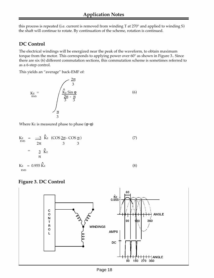
The electrical windings will be energized near the peak of the waveform, to obtain maximumtorque from the motor. This corresponds to applying power over 60° as shown in Figure 3.. Sincethere are six (6) different commutation sections, this commutation scheme is sometimes referred toas a 6-step control.

This yields an “average” back-EMF of:

2π3

KE = KE Sin φ (6)RMS 2π - π

3 3

π3

KE = —3 KE (COS 2π - COS π ) (7)RMS

2π 3 3

= 3 KE

π

KE = 0.955 KE (8)RMS

Where KE is measured phase to phase (φ−φ)

^

^

^

^

Figure 3. DC Control

Page 19

Application Notes

Thus, the expression for torque, with a floating neutral, becomes:

T = KTI (9)

T = 0.955 KEφφ I (Torque in N-m, KE in v/r/s) (10)

The back-EMF or voltage constant is measured phase to phase, and current is the DC level thru thewinding.

With the commutation scheme above, the maximum torque developed occurs at 60°, and is:

TMAX = T (sin(60)-sin(300)) (11)

= T x 1.73

The minimum torque is:

TMIN = T x 1.5 (12)

Therefore, theoretical torque ripple in this situation is:

% = MAX - MIN = 1.73 - 1.5 = 13.2% (13)MAX 1.73

Torque ripple depends on the control scheme, and it has to be designed to acceptable applicationtolerances.

AC Control

The application of a sinusoidal current:

I = I x (Sin φ + φ phase) (14)

is applied to all three windings (see Figure 4), which are sinusoidal:

KT = KTφ sin φ (15)

When energizing all three windings, the output torque developed is then equal to the sum of thetorques in all three windings:

TM = TR + TS + TT (16)

^

^

^

^

Figure 4. AC Control

^

Page 20

Application Notes

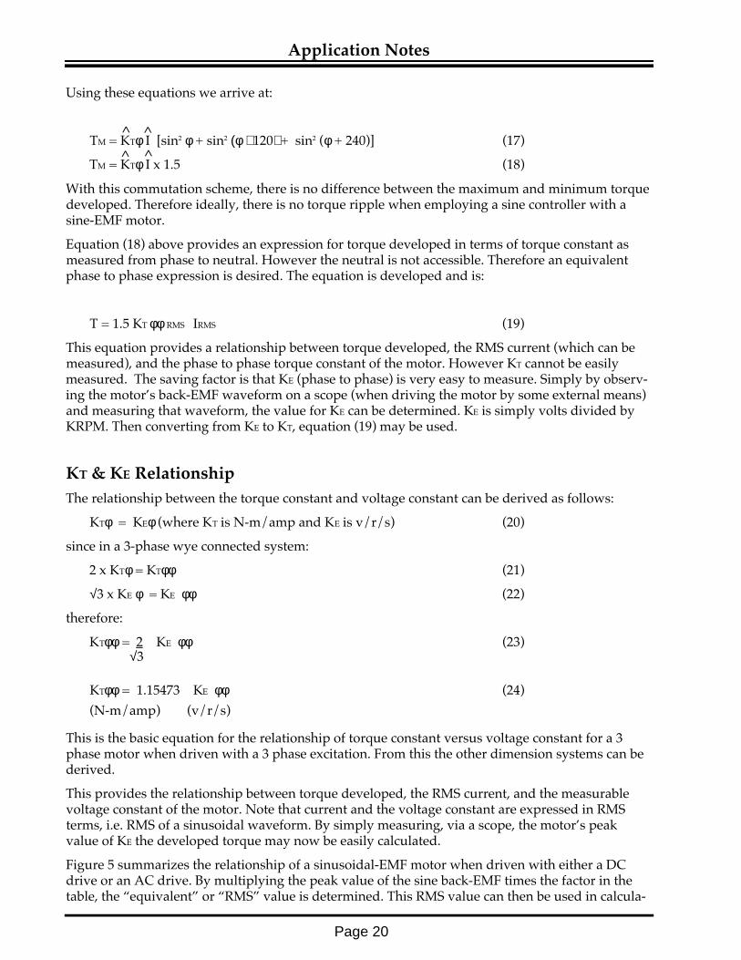
Using these equations we arrive at:

TM = KTφ I [sin2 φ + sin2 (φ +120) + sin2 (φ + 240)] (17)

TM = KTφ I x 1.5 (18)

With this commutation scheme, there is no difference between the maximum and minimum torquedeveloped. Therefore ideally, there is no torque ripple when employing a sine controller with asine-EMF motor.

Equation (18) above provides an expression for torque developed in terms of torque constant asmeasured from phase to neutral. However the neutral is not accessible. Therefore an equivalentphase to phase expression is desired. The equation is developed and is:

T = 1.5 KT φφ RMS IRMS (19)

This equation provides a relationship between torque developed, the RMS current (which can bemeasured), and the phase to phase torque constant of the motor. However KT cannot be easilymeasured. The saving factor is that KE (phase to phase) is very easy to measure. Simply by observ-ing the motor’s back-EMF waveform on a scope (when driving the motor by some external means)and measuring that waveform, the value for KE can be determined. KE is simply volts divided byKRPM. Then converting from KE to KT, equation (19) may be used.

KT & KE Relationship

The relationship between the torque constant and voltage constant can be derived as follows:

KTφ = KEφ (where KT is N-m/amp and KE is v/r/s) (20)

since in a 3-phase wye connected system:

2 x KTφ = KTφφ (21)

√3 x KE φ = KE φφ (22)

therefore:

KTφφ = 2 KE φφ (23) √3

KTφφ = 1.15473 KE φφ (24)

(N-m/amp) (v/r/s)

This is the basic equation for the relationship of torque constant versus voltage constant for a 3phase motor when driven with a 3 phase excitation. From this the other dimension systems can bederived.

This provides the relationship between torque developed, the RMS current, and the measurablevoltage constant of the motor. Note that current and the voltage constant are expressed in RMSterms, i.e. RMS of a sinusoidal waveform. By simply measuring, via a scope, the motor’s peakvalue of KE the developed torque may now be easily calculated.

Figure 5 summarizes the relationship of a sinusoidal-EMF motor when driven with either a DCdrive or an AC drive. By multiplying the peak value of the sine back-EMF times the factor in thetable, the “equivalent” or “RMS” value is determined. This RMS value can then be used in calcula-

^ ^

^ ^

Page 21

Application Notes

tions and current is calculated from the relationship:

T = KT I

where KT is the torque constant from Figure 5.

As an example, suppose you measure the sinusoidal waveform as 75 V/KRPM peak.

For a DC drive, the equivalent voltage constant is 71.2 V/KRPM; the torque constant would be 96.3oz-in/amp; and the current required to develop 180 lb-in of torque is:

T = KTI

180 = 96.3 I (Note: Divide 96.3 oz-in/amp by 16 to obtain lb-in/amp)16

or I= 29.9 amps

For an AC drive, the equivalent voltage constant is 53 V/KRPM; the torque constant would be124.2 oz-in/amps; and the current required to develop 180 lb-in of torque is:

T = KTI

180 = 124.2 I16

or I = 23 amps

Conclusion

Torques developed by the brushless motor depends upon the control technology used. An easyway to determine the type of control is to look at the feedback scheme. The DC control typicallyuses Hall sensors for feedback, where the AC control typically uses resolvers.

Voltage constant is measured as V/KRPM peak (phase to phase). The RMS values are determinedby multiplying by the value in the table:

English Metric

For DC drive KE 0.95 V/KRPM 0.009076 v/r/s

KT 1.285 oz-in/amp 0.009076 N-m/amp

For Sine drive KE 0.707 V/KRPM 0.006754 v/r/s

KT 1.656 oz-in/amp 0.011698 N-m/amp

Figure 5. Relationship between KE and KT for a brushless motor whendriven with a DC control versus an AC control

Page 22

Application Notes

Consider matching load and motor inertia. The followingpresents some points to consider.

System performance depends upon the load and motor coupling, and the ratio selected. Thesedetermine response, mechanical resonance, and power dissipated.

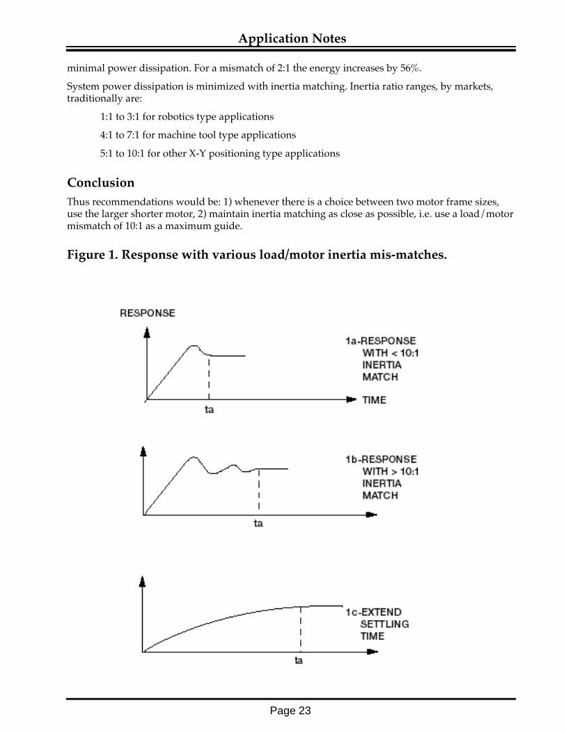
Response

Typical system response with “relatively good inertial matching” is shown in Figure 1. As the loadto motor mismatch is increased, oscillations occur, and it takes longer to settle in position(Figure 1b).

The fix, to prevent oscillation and overshooting, is to lower the gain and extend the settling time(Figure 1c). This leads to lower accelerations and slower positioning. This approach may not beacceptable for some applications.

Special loop compensation, of course, can be designed. This would allow handling of higherinertial mis-matches. However, this leads to highly custom designs and now standard off the shelfcontrols cannot be used.

Mechanical Resonance

Analyzing the transfer function of the load, motor shaft, and feedback device, the resultantequation is:

Where JL is the load inertia, JM is the motor inertia, and K is the transmission stiffness.

This equation provides the frequency of the mechanical resonance. It points out that the torsionalresonance 1) depends upon the load and motor coupling, i.e. the transmission stiffness and 2) thefrequency point is lower for high inertia loads.

For the best response, this resonant point should be outside the system bandwidth. It is typical tohave the resonant frequency 5-10 times the servo loop bandwidth due to rise time requirements.

The easiest, quickest, and least expensive method is to use gearing, or a larger motor (with moreinertia) to improve the inertia ratio.

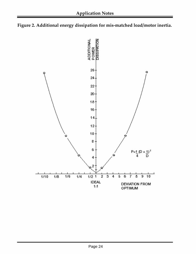
Power Dissipation

Analyzing the equation for energy dissipation for optimum versus non-optimum ratios, the resul-tant analysis is plotted in Figure 2. This show the amount of additional system energy dissipated asmis-match increases. It indirectly also reveals the additional current required (by the square root).

The plot reveals that a small deviation from optimum is not critical, however, as the deviationincreases, the penalty becomes increasingly severe. As can be seen, the ratio of 1:1 provides for

Inertia Matching

Îããããf = 1 (JL + JM) K2π JLJM

Page 23

Application Notes

minimal power dissipation. For a mismatch of 2:1 the energy increases by 56%.

System power dissipation is minimized with inertia matching. Inertia ratio ranges, by markets,traditionally are:

1:1 to 3:1 for robotics type applications

4:1 to 7:1 for machine tool type applications

5:1 to 10:1 for other X-Y positioning type applications

Conclusion

Thus recommendations would be: 1) whenever there is a choice between two motor frame sizes,use the larger shorter motor, 2) maintain inertia matching as close as possible, i.e. use a load/motormismatch of 10:1 as a maximum guide.

Figure 1. Response with various load/motor inertia mis-matches.

Page 24

Application Notes

Figure 2. Additional energy dissipation for mis-matched load/motor inertia.

Page 25

Application Notes

Conversion Tables

Rotary inertia (To convert from A to B, multiply by entry in table)

Conversion Tables

Torque (To convert from A to B, multiply by entry in table)

B lb-ft-s2

A or

gm-cm2 oz-in2 gm-cm-s2 kg-cm2 lb-in2 oz-in-s2 lb-ft2 Kg-cm-s2 lb-in-s2 slug-ft2

gm-cm2 1 5.46x10-3 1.01x10-3 10-3 3.417x10-4 1.41x10-5 2.37x10-6 1.01x10-6 8.85x10-7 7.37x10-8

oz-in2 182.9 1 0.186 0.182 0.0625 2.59x10-3 4.34x10-4 1.86x10-4 1.61x10-4 1.34x10-5

gm-cm-s2 980.6 5.36 1 0.9806 0.335 1.38x10-2 2.32x10-3 10-3 8.67x10-4 7.23x10-5

Kg-cm2 1000 5.46 1.019 1 0.3417 1.41x10-2 2.37x10-3 1.019x10-3 8.85x10-4 7.37x10-5

lb-in2 2.92x103 16 2.984 2.926 1 4.14x10-2 6.94x10-3 2.98x10-3 2.59x10-3 2.15x10-4

oz-in-s2 7.06x104 386.08 72 70.615 24.13 1 0.1675 7.20x10-2 6.25x10-2 5.20x10-3

lb-ft2 4.21x105 2304 429.71 421.40 144 5.967 1 0.4297 0.3729 3.10x10-2

Kg-cm-s2 9.8x105 5.36x103 1000 980.66 335.1 13.887 2.327 1 0.8679 7.23x10-2

lb-in-s2 1.129x106 6.177x103 1.152x103 1.129x103 386.08 16 2.681 1.152 1 8.33x10-2

lb-ft-s2

or 1.355x107 7.41x104 1.38x104 1.35x104 4.63x103 192 32.17 13.825 12 1

slug-ft2

B

A dyne-cm gm-cm oz-in kg-cm lb-in Newton-m lb-ft Kg-cm

dyne-cm 1 1.019x10-3 1.416x10-5 1.0197x10-6 8.850x10-7 10-7 7.375x10-8 1.019x10-8

gm-cm 980.65 1 1.388x10-2 10-3 8.679x10-4 9.806x10-5 7.233x10-5 10-5

oz-in 7.061x104 72.007 1 7.200x10-2 6.25x10-2 7.061x10-3 5.208x10-3 7.200x10-4

Kg-cm 9.806X105 1000 13.877 1 0.8679 9.806X10-2 7.233X10-2 10-2

lb-in 1.129x106 1.152x103 16 1.152 1 0.112 8.333x10-2 1.152x10-2

Newton-m 107 1.019x104 141.612 10.197 8.850 1 0.737 0.101

lb-ft 1.355x107 1.382x104 192 13.825 12 1.355 1 0.138

Kg-m 9.806x107 105 1.388x103 100 86.796 9.806 7.233 1

Page 26

Application Notes

Conversion Tables

Multiply By To Obtain

Length

Angstrom units 3.937 x 10-9 in.cm 0.3937 in.ft 0.30480 min. (U.S.) 2.5400058 cmin. (British) 0.9999972 in. (U.S.)m 1010 Angstrom unitsm 3.280833 ftm 39.37 in.m 1.09361 ydm 6.2137 x 10-4 miles (U.S. statute)yd 0.91440 m

miles (U.S. statute) 5,280 ft

Area

cir mils 7.854 x 10-7 in.2

cm2 1.07639 x 10-3 ft 2

cm2 0.15499969 in.2

ft2 0.092903 m2

ft2 929.0341 cm2

in.2 6.4516258 cm2

Volume

cm3 3.531445 x 10-5 ft3

cm3 2.6417 x 10-4 gal (U.S.)cm3 0.033814 oz (U.S. fluid)ft3 (British) 0.9999916 ft3

ft3 (U.S.) 28.31625 L (liter)m3 264.17 gal (U.S.)gal (British) 4,516.086 cm3

gal (British) 1.20094 gal (U.S.)gal (U.S.) 0.13368 ft3 (U.S.)gal (U.S.) 231 in.3

gal (U.S.) 3.78533 L (liter)gal (U.S.) 128 oz (U.S. fluid)oz (U.S. fluid) 29.5737 cm3

oz (U.S. fluid) 1.80469 in.3

yd3 0.76456 m3

yd3 (British) 0.76455 m3

Plane Angle

radian 57.29578 deg

Weight

Dynes 2.24809 x 10-6 lbkg 35.2740 oz (avoirdupois)kg 2.20462 lbkg 0.001 tons (metric)kg 0.0011023 tons (short)oz (avoirdupois) 28.349527 gramstons (long) 1,106 kgtons (long) 2,240 lbtons (metric) 1,000 kgtons (metric) 2,204.6 lbtons (short) 2,000 lb

Page 27

Application Notes

Page 28

Application Notes

BALDOR ELECTRIC COMPANYP. O. BOX 2400

Fort Smith, Arkansas 72901-2400(501) 646-4711

Fax (501) 648-5792www.baldor.com

Printed in U.S.A.2/99 FARR 5000

© 99 Baldor Electric CompanyMN1200