Embed Size (px)
Citation preview

More repeated measures

More complex repeated measures
• As with our between groups ANOVA, we can also have more than one repeated measures factor
• 2-way repeated measures
Two way repeated measures
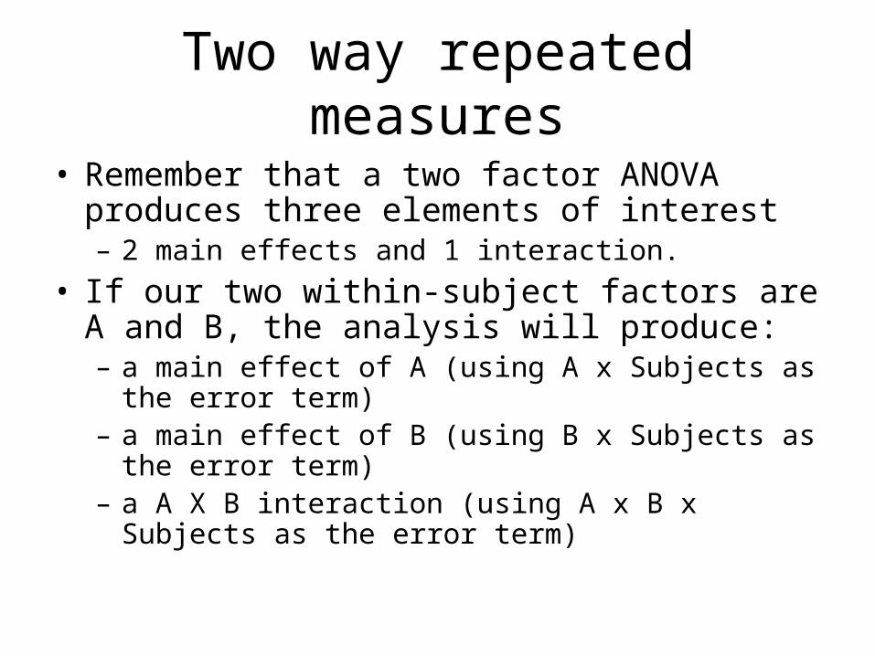
• Remember that a two factor ANOVA produces three elements of interest– 2 main effects and 1 interaction.
• If our two within-subject factors are A and B, the analysis will produce:– a main effect of A (using A x Subjects as the error
term)– a main effect of B (using B x Subjects as the error
term)– a A X B interaction (using A x B x Subjects as the
error term)

Example
• An experiment designed to look at the effects of therapy on self-esteem
• Subjects self-esteem measures
• 5 subjects
• One within-subject effect with 4 levels (weeks 1-4)
• Another with 2 levels (wait,therapy)

Baseline Therapy
1 2 3 4 1 2 3 4
3 5 9 6 5 6 11 7
7 11 12 11 10 12 18 15
9 13 14 12 10 15 15 14
4 8 11 7 6 9 13 9
1 3 5 4 3 5 9 7
Data
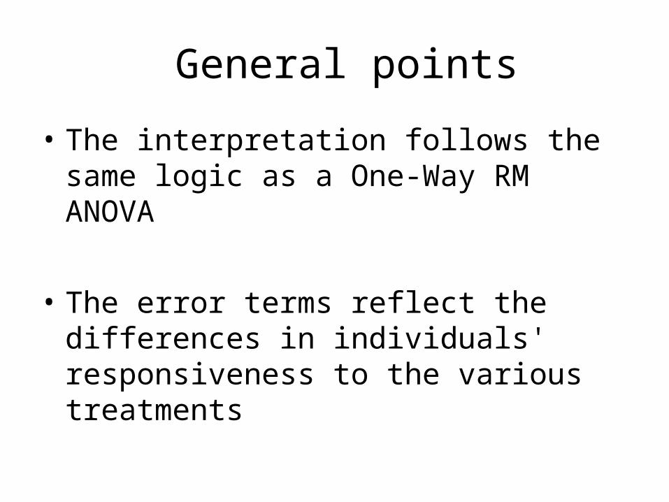
• The interpretation follows the same logic as a One-Way RM ANOVA
• The error terms reflect the differences in individuals' responsiveness to the various treatments
General points

Partitioning the effects
• Recall from the one-way RM design that our error term was a reflection of how different subjects respond differently to different treatments – Treatment X subject interaction
• The variance within people was a combination of the treatment effect, the interaction w/ subjects, and random error
• The error term in that situation contained both the interaction effects and random error
Partitioning the effects
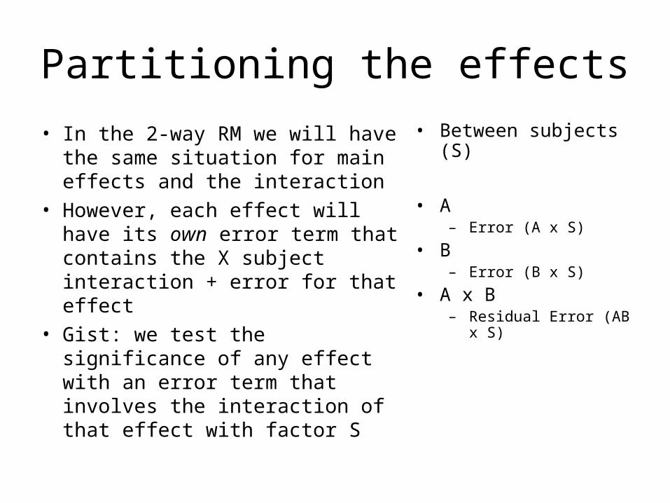
• In the 2-way RM we will have the same situation for main effects and the interaction
• However, each effect will have its own error term that contains the X subject interaction + error for that effect
• Gist: we test the significance of any effect with an error term that involves the interaction of that effect with factor S
• Between subjects (S)
• A– Error (A x S)
• B– Error (B x S)
• A x B– Residual Error (AB x S)
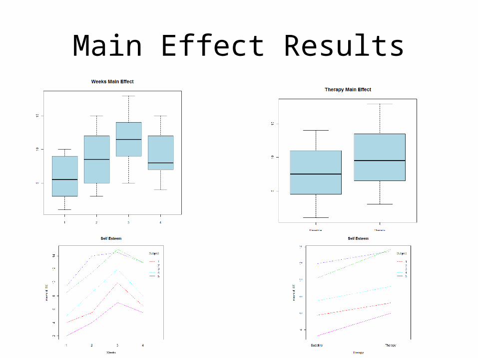
Main Effect Results

Interaction Results
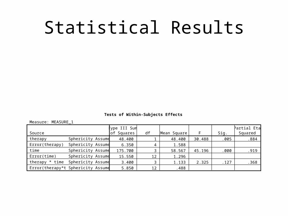
Statistical Results
Tests of Within-Subjects Effects
Measure: MEASURE_1
48.400 1 48.400 30.488 .005 .884
6.350 4 1.588
175.700 3 58.567 45.196 .000 .919
15.550 12 1.296
3.400 3 1.133 2.325 .127 .368
5.850 12 .488
Sphericity Assumed
Sphericity Assumed
Sphericity Assumed
Sphericity Assumed
Sphericity Assumed
Sphericity Assumed
Sourcetherapy
Error(therapy)
time
Error(time)
therapy * time
Error(therapy*time)
Type III Sumof Squares df Mean Square F Sig.
Partial EtaSquared
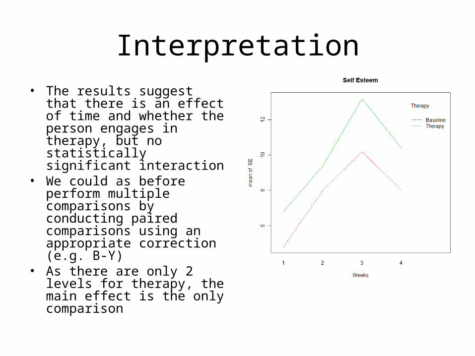
Interpretation• The results suggest that there
is an effect of time and whether the person engages in therapy, but no statistically significant interaction
• We could as before perform multiple comparisons by conducting paired comparisons using an appropriate correction (e.g. B-Y)
• As there are only 2 levels for therapy, the main effect is the only comparison

Interpretation
• Technically, a significant interaction is not required to test for simple effects– Plus in this case we had an interesting effect size for
the interaction anyway• Note that this is for demonstration only, with
main effects both significant and non significant interaction you should not perform simple effects analysis– But even that suggestion is based on p-values so…
• The error term will be the interaction of the effect X subject at the particular level for the other within subjects factor (e.g. A x S at B1)

Simple Effects
Pairwise Comparisons
Measure: MEASURE_1
-2.000* .316 .003 -2.878 -1.122
2.000* .316 .003 1.122 2.878
-1.400* .245 .005 -2.080 -.720
1.400* .245 .005 .720 2.080
-3.000* .894 .028 -5.483 -.517
3.000* .894 .028 .517 5.483
-2.400* .510 .009 -3.816 -.984
2.400* .510 .009 .984 3.816
(J) therapy2
1
2
1
2
1
2
1
(I) therapy1
2
1
2
1
2
1
2
time1
2
3
4
MeanDifference
(I-J) Std. Error Sig.a
Lower Bound Upper Bound
95% Confidence Interval forDifference
a
Based on estimated marginal means
The mean difference is significant at the .05 level.*.
Adjustment for multiple comparisons: Least Significant Difference (equivalent to no adjustments).a.
Pairwise Comparisons
Measure: MEASURE_1
-3.200* .490 .003 -4.560 -1.840
-5.400* .510 .000 -6.816 -3.984
-3.200* .200 .000 -3.755 -2.645
3.200* .490 .003 1.840 4.560
-2.200* .583 .020 -3.819 -.581
.000 .447 1.000 -1.242 1.242
5.400* .510 .000 3.984 6.816
2.200* .583 .020 .581 3.819
2.200* .583 .020 .581 3.819
3.200* .200 .000 2.645 3.755
.000 .447 1.000 -1.242 1.242
-2.200* .583 .020 -3.819 -.581
-2.600* .678 .019 -4.483 -.717
-6.400* .510 .000 -7.816 -4.984
-3.600* .510 .002 -5.016 -2.184
2.600* .678 .019 .717 4.483
-3.800* 1.020 .020 -6.631 -.969
-1.000 .707 .230 -2.963 .963
6.400* .510 .000 4.984 7.816
3.800* 1.020 .020 .969 6.631
2.800* .583 .009 1.181 4.419
3.600* .510 .002 2.184 5.016
1.000 .707 .230 -.963 2.963
-2.800* .583 .009 -4.419 -1.181
(J) time2
3
4
1
3
4
1
2
4
1
2
3
2
3
4
1
3
4
1
2
4
1
2
3
(I) time1
2
3
4
1
2
3
4
therapy1
2
MeanDifference
(I-J) Std. Error Sig.a
Lower Bound Upper Bound
95% Confidence Interval forDifference
a
Based on estimated marginal means
The mean difference is significant at the .05 level.*.
Adjustment for multiple comparisons: Least Significant Difference (equivalent to noadjustments).
a.
Another example
• Habituation in mice• Habituation represents the simplest form of learning
– Decline in the tendency to respond to stimuli that have become familiar due to repeated exposure
• For example, a sudden noise may initially elicit reaction, but if we hear it repeatedly, we gradually get use to it so that we are less startled the second time we hear it and eventually just ignore it
• If stimulus is withheld for some period following habituation, the response will recover– Extinction and return

Meces
• Mice were placed in a chamber and presented with a startle tone for 50 trials, and startle response was recorded
• Then they were given a 30 minute break and run again
• Data broken down into 5 blocks of 10 trials each for each session, and it is the blocks that will be analyzed
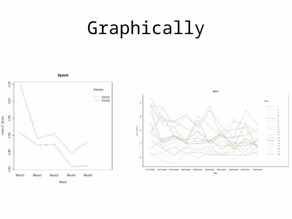
Graphically
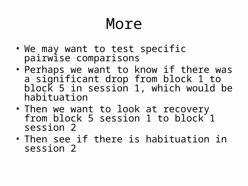
More
• We may want to test specific pairwise comparisons
• Perhaps we want to know if there was a significant drop from block 1 to block 5 in session 1, which would be habituation
• Then we want to look at recovery from block 5 session 1 to block 1 session 2
• Then see if there is habituation in session 2
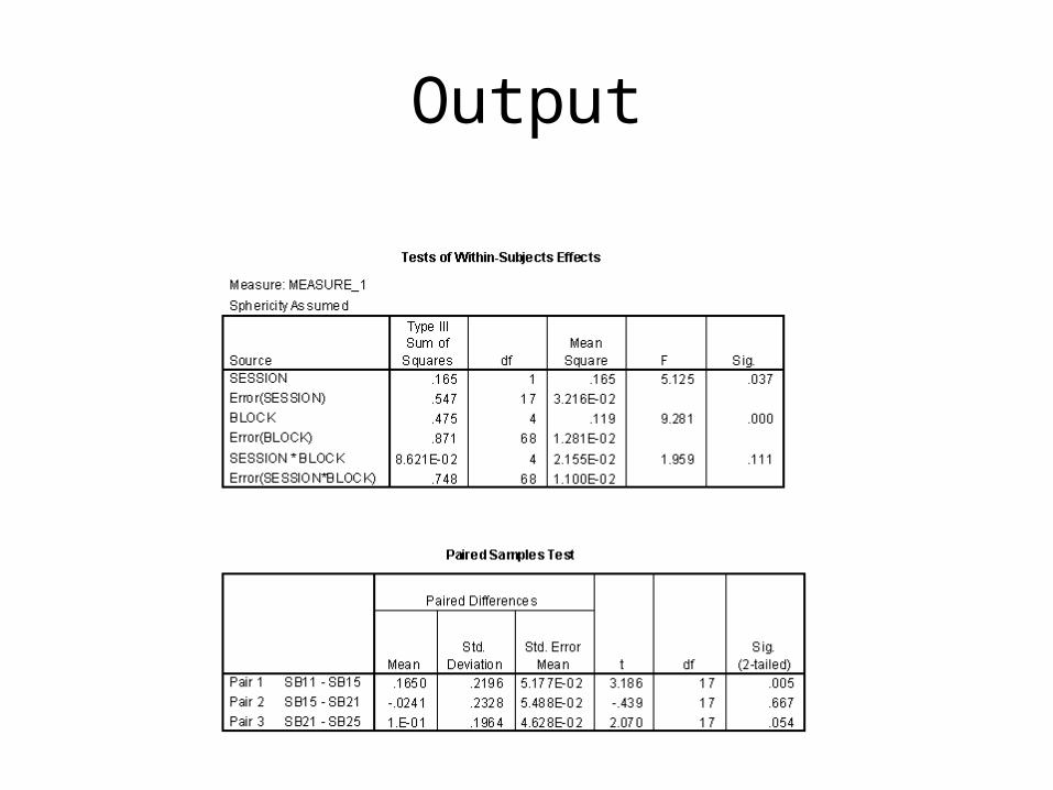
Output

Contrasts
• Perhaps instead we wanted to test a specific type of contrast– Recall difference, repeated, helmert etc.
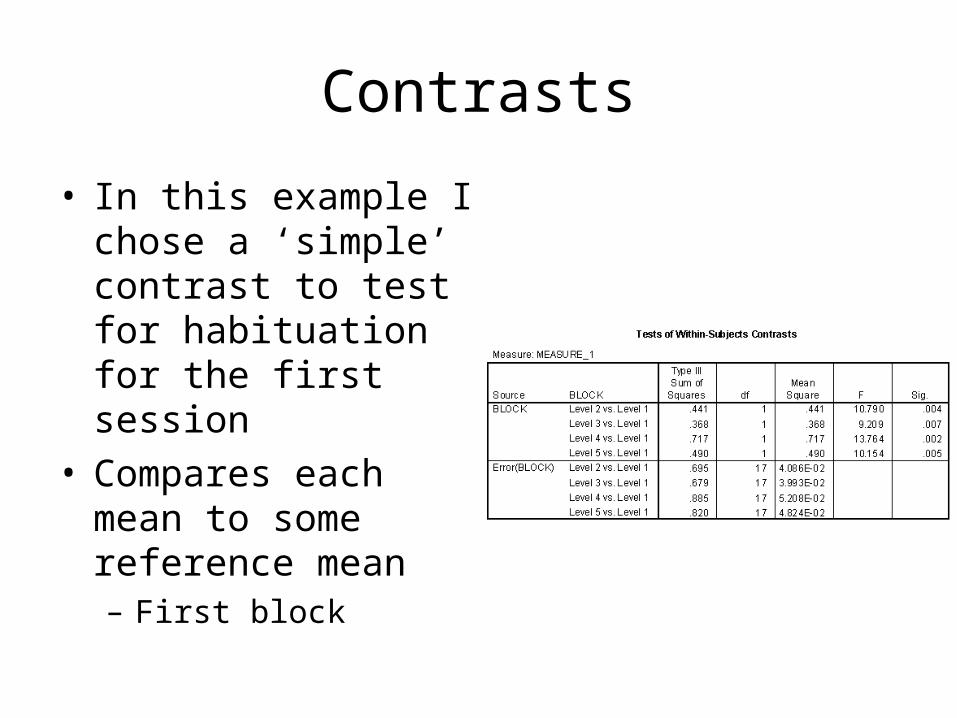
Contrasts
• In this example I chose a ‘simple’ contrast to test for habituation for the first session
• Compares each mean to some reference mean – First block
More complex
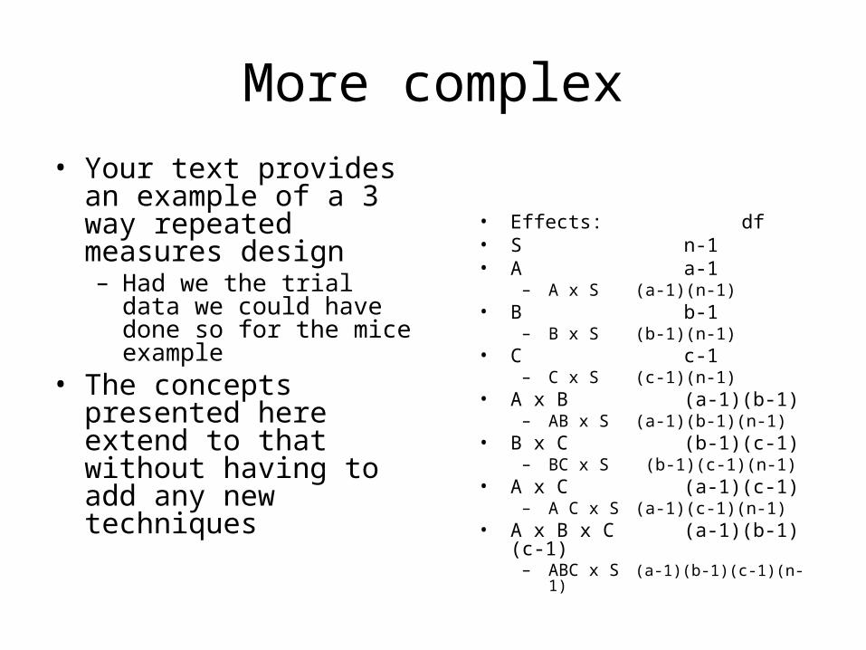
• Your text provides an example of a 3 way repeated measures design– Had we the trial data we
could have done so for the mice example
• The concepts presented here extend to that without having to add any new techniques
• Effects: df• S n-1• A a-1
– A x S (a-1)(n-1)• B b-1
– B x S (b-1)(n-1)• C c-1
– C x S (c-1)(n-1)• A x B (a-1)(b-1)
– AB x S (a-1)(b-1)(n-1)• B x C (b-1)(c-1)
– BC x S (b-1)(c-1)(n-1)• A x C (a-1)(c-1)
– A C x S (a-1)(c-1)(n-1)• A x B x C (a-1)(b-1)(c-1)
– ABC x S (a-1)(b-1)(c-1)(n-1)
Appendix
Data setup
• Now setting up the data in SPSS follows the same general system – Each row representing a single subject
• The analysis itself is run in the same way as a One-Way RM design, except now we specify 2 factors. [Analyze General Linear Model Repeated Measures]
SPSS simple effects
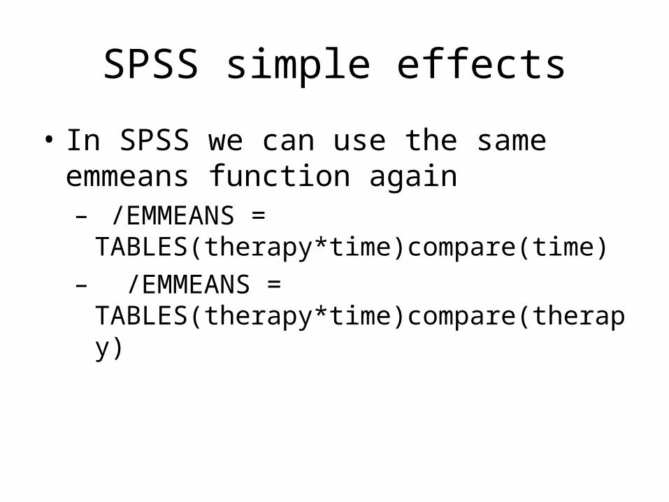
• In SPSS we can use the same emmeans function again– /EMMEANS =
TABLES(therapy*time)compare(time)– /EMMEANS =
TABLES(therapy*time)compare(therapy)

Mice example in SPSS