Monomethylamine–water vapour absorption refrigeration system

www.elsevier.com/locate/apthermeng

Applied Thermal Engineering 25 (2005) 867–876

Monomethylamine–water vapour absorptionrefrigeration system

R.J. Romero a,*, Luis Guillen b, I. Pilatowsky c

a Centro de Investigacion en Ingenierıa y Ciencias Aplicadas, UAEM, Av. Universidad 1001, Chamilpa,

CP 62210 Cuernavaca, Morelos, Mexicob Posgrado en Ingenierıa—Area Energıa, UNAM, apartado postal 34, 62580 Temixco, Morelos, Mexico

c Centro de Investigacion en Energıa, UNAM, apartado postal 34, 62580 Temixco, Morelos, Mexico

Received 30 September 2003; accepted 19 August 2004

Abstract

Thermodynamic equations for the performance evaluation of the monomethylamine–water vapour

absorption refrigeration system have been obtained, analysed and reported in this paper. These equationshave been derived from experimental data with a good agreement with the expected values and have been

expressed in polynomial form. These equations were utilized on the energy and mass balances for obtaining

the coefficient of performance (COP) with this pair and compared with the ammonia–water absorption sys-

tem. It has been observed that this refrigerant–absorbent pair has a greater coefficient of performance at

low generation temperatures and moderate condenser, absorber and evaporator temperatures.

� 2004 Published by Elsevier Ltd.

Keywords: Monomethylamine water solutions; Absorption refrigeration cycle; Thermodynamic equations

1. Introduction

In absorption refrigeration cycles it is very important to select the appropriate absorbent–refrigerant pair. Many promising combinations have been proposed [6]. Evaluation of potential

1359-4311/$ - see front matter � 2004 Published by Elsevier Ltd.

doi:10.1016/j.applthermaleng.2004.08.007

* Corresponding author.

E-mail address: [email protected] (R.J. Romero).

mailto:[email protected]

Nomenclature

COP coefficient of performance (dimensionless)CP specific heat (kJkg�1�C�1)h specific enthalpy (kJkg�1)m mass flow rate (kgh�1)P pressure (atm)Q heat flow rate (kJh�1)T temperature (K)Tr relative temperature (�C)X weight concentration (%)

SubscriptsA absorberC condenserE evaporatorSHE solution heat exchangerG generatorL liquidR rectifierS concentrated solutionSat saturatedShe superheatedV vapourW diluted solution

868 R.J. Romero et al. / Applied Thermal Engineering 25 (2005) 867–876

working fluid for the absorption cycle is a problem because of a lack of published thermodynamicdata. The ideal absorbent–refrigerant pair does not exist, all possible combinations present advan-tages and disadvantages. Nevertheless, it is recommended to keep the pressure in the system at thelowest possible level to achieve low generating temperatures. The most widely used fluid pairs areammonia–water and lithium bromide–water. Among different options of refrigerants that can beused, monomethylamine can be combined with liquid absorbents, such as water, thiocyanates, etc.

The vapour pressures and generating temperature data of the monomethylamine–water solu-tions show that it is possible to use low temperature thermal energy sources such as solar, geother-mal, industrial and commercial waste heat [2,1,4].

The derivate state equations obtained from experimental data are the main contribution of thispaper, which can be used for absorption refrigeration cycle thermodynamic calculations.

In this work, thermodynamic data, such as the vapour pressure, liquid and vapour saturatedenthalpy and superheated vapour enthalpy of pure monomethylamine have been shown [5] andvapour pressure, liquid and vapour enthalpy of monomethylamine–water solutions have beenexpressed in a polynomial form. The state equations for monomethylamine–water solutions werederived from pressure–concentration–temperature and enthalpy–concentration diagrams [1,7]

R.J. Romero et al. / Applied Thermal Engineering 25 (2005) 867–876 869

together with the corresponding state equations previously reported [3] with a good agreementwith the experimental results.

2. Single-stage absorption refrigeration cycle

2.1. Description

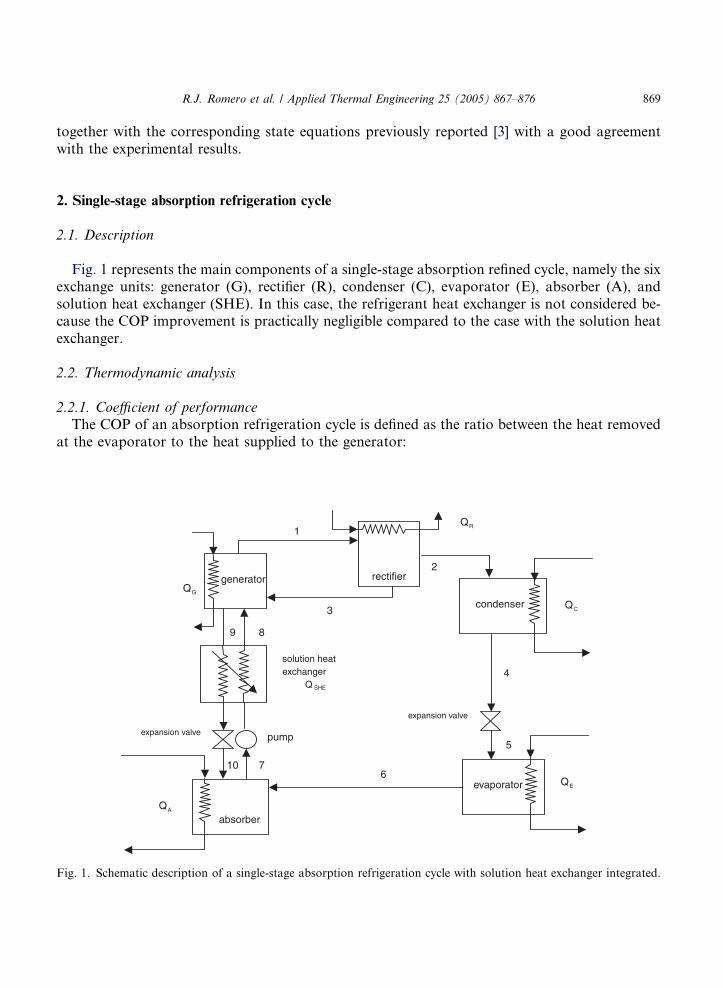
Fig. 1 represents the main components of a single-stage absorption refined cycle, namely the sixexchange units: generator (G), rectifier (R), condenser (C), evaporator (E), absorber (A), andsolution heat exchanger (SHE). In this case, the refrigerant heat exchanger is not considered be-cause the COP improvement is practically negligible compared to the case with the solution heatexchanger.

2.2. Thermodynamic analysis

2.2.1. Coefficient of performanceThe COP of an absorption refrigeration cycle is defined as the ratio between the heat removed

at the evaporator to the heat supplied to the generator:

QR1

rectifiergenerator2

QG

condenser QC3

9 8

solution heat exchanger

Q4

expansion valve

expansion valve

pump5

10 7

evaporator6

QE

absorberQA

SHE

Fig. 1. Schematic description of a single-stage absorption refrigeration cycle with solution heat exchanger integrated.


COP ¼ QE

QG

ð1Þ

The theoretical calculations of COP have been performed with the known values of generator,absorber, condenser, evaporator and rectifier temperatures and some basic assumptions areestablished:

(1) The temperature of the condenser, evaporator, absorber, generator and rectifier is uniformthroughout the components.

(2) The refrigerant vapour is in thermodynamic equilibrium with the concentrated solutionentering from the absorber and diluted solution leaving the generator.

(3) The diluted solution leaving the generator is at the same temperature and concentration atthe generator and it is in thermodynamic equilibrium.

(4) The refrigerant fraction leaving the generator can be considered as vapour whose concentra-tion is less that 1.

(5) Considered perfect rectification of vapour leaving the rectifier and the refrigerant vapour isassumed to be in the pure state.

(6) The concentrated solution leaving the rectifier to the generator is saturated liquid at the tem-perature and concentration of the rectifier.

(7) The concentrated solution leaving the absorber is saturated liquid at the temperature andconcentration that are the same in the absorber.

(8) The effectiveness of the heat exchangers is also assumed to be known.(9) The heat losses to ambient, the pressure drops and the work required and the temperature

rise due to heat rejected by the pump solution were assumed to be negligible.(10) As the same cooling medium is used, the absorber and condenser temperatures are assumed

to have the same value.(11) The heat exchanger efficiency gEX is assumed to be 70% [3].

2.2.2. AnalysisThe main equations used for calculation of the mass and energy balance for each component

of the refrigeration cycle within the above assumptions and referring to Fig. 1 are the following:

(1) Generator

QG ¼ m1h1 þ m9h9 � m8h8 � m3h3 ð2Þ
(2) Rectifier
QR ¼ m2h2 þ m3h3 � m1h1 ð3Þ
(3) Condenser
QC ¼ m4h4 � m2h2 ð4Þ
(4) Evaporator
QE ¼ m6h6 þ m5h5 ð5Þ


(5) Absorber

QA ¼ m7h7 þ m6h6 � m10h10 ð6Þ
(6) Solution heat exchanger
QSHE ¼ mW h8 � h7ð Þ ¼ mS h10 � h9ð Þ ð7Þ

2.2.3. Equations for thermodynamic properties2.2.3.1. Monomethylamine–water solutions equations. The experimental data were obtained from apressure range of 0.2 to 8.4 atm and �26 �C to 150�C, for all of the concentration range.

Pressure–concentration–temperature equation

P ¼ ae½bð�1=TÞ� ð8Þ
where
a ¼ f ðxÞ ¼X6

i¼0

aixi ð9Þ

and

b ¼ f ðxÞ ¼X3

i¼0

bixi ð10Þ

Coefficients for Eq. (9)

a0 = 786,778.05
a1 = �1,844,610.00 a2 = 562,720.14 a3 = 1.752200.00 a4 = �1,124,410.00

b0 = 5054.24
b1 = �2694.00 b2 = �1409.40 b3 = 2186.33
Vapour enthalpy

hV ¼ f ðxVÞ ¼ 4:1868X2

i¼0

cixiV ð11Þ

cðiÞ ¼ f ðP Þ ¼ dði; 0Þ þ dði; 1ÞP þ dði; 2ÞP 2 ð12Þ


d(0,0) = 628.78226
d(0,1) = �3.08167 d(0,2) = �0.00688 d(1,0) = 9.07855 d(1,1) = �0.01875 d(1,2) = 0.0000179439 d(2,0) = �0.56553 d(2,1) = 0.00144 d(2,2) = �2.84255E�07


Liquid enthalpy

Coeffi

hL ¼ f ðxLÞ ¼X6

i¼0

eðiÞxiL ð13Þ

in this equation, each e(i) coefficient must be calculated by the next correlation.

eðiÞ ¼ f ðT Þ ¼X6

j¼0

f ði; jÞTrj ð14Þ

cients for Eq. (14)

f(0,0) = 0.46384
f(1,0) = �0.87087 f(2,0) = �0.03016 f(3,0) = 0.00265 f(4,0) = �0.000060575 f(5,0) = 7.10325E�07 f(6,0) = �3.65449E�09 f(0,1) = 0.99636 f(1,1) = 0.02883 f(2,1) = �0.00239 f(3,1) = 7.20938E�05 f(4,1) = �1.01432E�06 f(5,1) = 6.25913E�09 f(6,1) = �1.05388E�11 f(0,2) = 0.00152 f(1,2) = �0.00069062 f(2,2) = 7.92131E�05 f(3,2) = �4.46748E�06 f(4,2) = 1.35161E�07 f(5,2) = �2.09847E�09 f(6,2) = 1.29714E�11 f(0,3) = �2.74545E�06 f(1,3) = �9.2258E�06 f(2,3) = 6.22817E�07 f(3,3) = �1.50223E�09 f(4,3) = �6.78505E�10 f(5,3) = 1.72135E�11 f(6,3) = �1.28729E�13 f(0,4) = �6.20206E�07 f(1,4) = 3.59394E�07 f(2,4) = �3.64231E�08 f(3,4) = 1.89392E�09 f(4,4) = �5.62633E�11 f(5,4) = 8.82903E�13 f(6,4) = �5.54129E�15 f(0,5) = 7.02407E�09 f(1,5) = �3.22044E�09 f(2,5) = 3.78385E�10 f(3,5) = �2.4713E�11 f(4,5) = 8.64566E�13 f(5,5) = �1.48831E�14 f(6,5) = 9.79809E�17 f(0,6) = �2.17536E�11 f(1,6) = 9.52048E�12 f(2,6) = �1.26477E�12 f(3,6) = 9.33127E�14 f(4,6) = �3.49466E�15 f(5,6) = 6.22654E�17 f(6,6) = �4.17075E�19
Monomethylamine–water vapour auxiliary equations

In order to calculate the vapor enthalpy as a function of leaving generator liquid concentra-tion, the following auxillary equation is proposed:

haux ¼ f ðxLÞ ¼X4

i¼0

gixiL ð15Þ

where:

gðiÞ ¼ f ðP Þ ¼ jðiÞ þ kðiÞeð�P=rsnðiÞÞ ð16Þ


j(0) = 676.12113
j(1) = �16.99847 j(2) = 0.28229 j(3) = �0.00182 j(4) = 1.59E�06 k(0) = �49.15441 k(1) = �11.41086 k(2) = 0.49219 k(3) = �0.00712 k(4) = 3.51E�05 rsn(0) = 1.51881 rsn(1) = 4.45503 rsn(2) = 4.35334 rsn(3) = 4.99016 rsn(4) = 6.29341


2.2.3.2. Monomethylamine refrigerant equations [5]. Vapour pressure

Coeffi

LnP ¼ A0 þA1

Tð17Þ


A0 = 11.34186

cients for Eq. (19)

A1 = �3006.263

Enthalpy of saturated liquid

hL ¼ D0 þ D1T þ D2T 2 ð18Þ


D0 = �18.33748
D1 = 72.50143 D2 = 0.001295105
Enthalpy of saturated vapour

hV ¼ F 0 þ F 1T þ F 2T 2 ð19Þ

F0 = 175.819
F1 = 0.4883584 F2 = �0.002264305
Enthalpy of superheated vapour

hVShe ¼ hV þ CPShe T She � T Sð Þ ð20Þ

3. Results

Fig. 2 shows experimental and calculated data with Eq. (8). This equation shows a good agree-ment for temperatures from �26 �C to 150 �C, weight concentrations between 0% and 100% andpressures from 0.2 to 8.4atm.

Fig. 3 presents the experimental and calculated data with Eq. (13), which shows a good agree-ment for the following range: weight concentrations between 0% and 60% and temperatures from�40�C to 120 �C. As can be seen at T = 140 �C, the equation shows a good agreement for 40%weight concentration or lower.

Fig. 4 shows that the COP values increase sharply until a maximum value is reached and afterthat the value diminishes smoothly on increasing the generation temperature and it also dimin-ishes on increasing the condensation and absorption temperatures. In the case of the ammo-nia–water solutions, the values of the COP are higher for generation temperatures above 80�Ccorresponding to TC = TA = 30�C and TG above 97 �C for temperatures of TC = TA = 40 �C.However, for generator temperatures between 60 and 83�C the monomethylamine–water

0.0001

0.001

0.01

0.1

1

10

100

_40 _20 0 20 40 60 80 100 120 140 160 180

Temperature T, (˚C)

Pre

ssu

re P

, (at

m)

x = 0 %x = 10 %x = 20 %x = 30 %x = 40 %x = 50 %x = 60 %x = 65 %

x = 100 %

Fig. 2. Vapour–pressure against temperature, comparison of experimental and calculated data with the equations

shown in this work.

–300

–200

–100

0

100

200

300

400

500

600

700

0 10 20 30 40 50 60

Weigth concentration, x (%w)

En

thal

py,

h (

kJ k

g-1

)

T = 140 ˚CT = 120 ˚CT = 100 ˚CT = 80 ˚CT = 60 ˚CT = 40 ˚CT = 20 ˚CT = 0 ˚CT = –20 ˚CT = –40 ˚C

Fig. 3. Enthalpy against concentration, comparison between experimental and calculated data.


0.00

0.10

0.20

0.30

0.40

0.50

0.60

0 20 40 60 80 100 120 140 160 180 200TG (°C)

CO

P (d

imen

sion

less

)

monomethylamine - water

ammonia - water

TC = 35 °C TC = 40 °C

TC = 30 °C

TC = 40 °C

TC = 30 °C

Fig. 4. Coefficient of performance COP for monomethylamine–water and ammonia–water solutions as a function of

generator temperature at three different absorber and condenser temperatures (25, 30 and 35 �C for monomethylamine–

water and 30, 40 �C for ammonia–water).


solutions have high values of COP, which makes possible the use of sources of low enthalpy, assolar energy, industrial waste heat, among others.

Fig. 3 shows a good correlation among the experimental values (marks) and the values obtainedwith the equations that are presented in this work (continuous lines); for this reason these equa-tions can be considered valid in the mentioned ranges.

It can be observed that the higher values of COP for the monomethylamine–water system isfound in a short range of generation temperatures between 63 and 80�C, with COP values from0.35 to 0.51, these are bigger than the corresponding ones in the ammonia–water system.

4. Discussion

With the correlated equations for pressure vapour and enthalpy for monomethylamine–watersolutions the energy balance was calculated and the COP was computed. These equations allowthe comparison of this pair with the ammonia–water system.

The monomethylamine–water system was computed in the temperature range from 60 to 100 �Cfor a range from 30 to 40�C of condensation temperature. With the proposed equations, the cal-culations of the COP for the monomethylamine–water system were carried out and these werecompared with the simulation under similar conditions with the ammonia–water system.


The ammonia–water system has a higher COP at higher temperatures and it declines as wellwhen the generation temperature increases.

5. Conclusion

The monomethylamine–water system is a good potential pair for refrigeration cycles forabsorption which can be operated at lower generation temperatures that allow the use of heatsources like solar, geothermal, industrial waste or others.

An additional advantage of the monomethylamine–water system is the lower vapour requiredpressures. This capability would allow slighter devices to require smaller wall thickness in thecomponents of the system.

Due to the normal boiling point of the monomethylamine (�6 �C) and to avoid vacuum oper-ation problems, this system can be used for air conditioning and product conservation purposes.

Acknowledgment

The author wishes to recognize the partial support for this research to UAEMOR-PTC-73project.

References

[1] E.A. Bonauguri, A. Bonfanti, V. Gurdjian, Gemische von CH3NH2 und H2O, Forschungen (Ricerche), No. 2,

Beihettz zu No. 5 der Zeitschrift, La Thermotecnica, 1954.

[2] W.A. Felsing, P.H. Wohlford, The heats of solution of gaseous methylamine, J. Am. Chem. Soc. 54 (1932) 1442–

1445.

[3] I. Pilatowsky, W. Rivera, R. Best, State equations for monomethylamine–water solutions, derived from equilibrium

diagrams, Non published internal report, No. LES 94-0504-104, Energy Solar Laboratory, IIM-UNAM, Temixco,

Morelos, Mexico, 1994.

[4] J.P. Roberson, C.Y. Lee, R.G. Squires, L.F. Albright, Vapour pressure of ammonia and monomethylamine in

solutions for absorption refrigeration systems, ASHRAE Trans. 72 (1) (1966) 198–208.

[5] K.P. Tyagi, Methylamine–sodium thiocyanate vapour absorption refrigeration, Heat Recov. Syst. & CHP 12 (3)

(1992) 283.

[6] K.P. Tyagi, Comparison of binary mixtures for absorption refrigeration systems, Heat Recov. Syst. 3 (1983) 421.

[7] T. Uemura, Y. Higuchi, S. Hasaba, Studies on the monomethylamine–water absorption refrigerating machine,

Refrigeration 42 (471) (1967) 2–13.

Documents

Monomethylamine–water vapour absorption refrigeration system