Embed Size (px)
Citation preview
ISSN 1612-6793Nr. ZFI-BM-2016-19
Master’s Thesissubmitted in partial fulfilment of the
requirements for the course “Applied Computer Science”
Monitoring Mechanism Design for a DistributedReconfigurable Onboard Computer
Tanyalak Vatinvises
Institute of Computer Science
Bachelor’s and Master’s Thesesof the Center for Computational Sciences
at the Georg-August-Universität Göttingen
15. August 2016


Georg-August-Universität GöttingenInstitute of Computer Science
Goldschmidtstraße 737077 GöttingenGermany
T +49 (551) 39-172000t +49 (551) 39-14403B [email protected] www.informatik.uni-goettingen.de
First Supervisor: Prof. Dr. Ramin Yahyapour, Georg-August-Universität GöttingenSecond Supervisor: Dr. rer.nat. Andreas Gerndt, German Aerospace Center (DLR)

I hereby declare that I have written this thesis independently without any help from others andwithout the use of documents or aids other than those stated. I have mentioned all used sourcesand cited them correctly according to established academic citation rules.
Göttingen, 15. August 2016
v
AbstractThe Onboard Computer - Next Generation (OBC-NG) project is initiated by the German Aerospace Center(DLR) to develop a distributed and reconfigurable onboard computer of Commercial off-the-shelf (COTS)components. Its goal is to utilize the higher computational power of COTS components and to maintainhigh system reliability, which is required for spacecraft. However, COTS have a lower robustness than thetraditional space-qualified components and therefore a higher probability of failures. Thus, a monitoringsystem is indispensable. This thesis focuses on the design of a monitoring system, to evaluate the healthstatus of the distributed components. It shall detect failures before any corrective action, e.g. migrating thetasks to the other functioning components, can be triggered.
Different monitoring techniques have different trade-offs, in terms of monitoring efficiency and monitoringoverhead. Initially, various monitoring concepts are investigated, in order to qualitatively analyze theirtrade-offs and designs. Three monitoring mechanisms, PULL, PUSH and PUSH-PULL, are selected andmodeled. Afterwards, the models are simulated on the discrete event simulator OMNeT++ and tested underdifferent environment as well as monitoring mechanism settings. The simulation results, which representa quantitative investigation of the designed monitoring mechanisms, are used to evaluate and comparethem. The derived verdicts are used to identify the most suitable mechanism and settings for the OBC-NGsystem. The results show that PUSH mechanism is more suitable for OBC-NG system than the currentlyimplemented PULL mechanism.

Contents
1 Introduction 11.1 Motivation and Problem Statement . . . . . . . . . . . . . . . . . . . . . . . . . . . . 11.2 Purpose and Goals . . . . . . . . . . . . . . . . . . . . . . . . . . . . . . . . . . . . . 21.3 Task . . . . . . . . . . . . . . . . . . . . . . . . . . . . . . . . . . . . . . . . . . . . . . 3
1.3.1 Research Phase . . . . . . . . . . . . . . . . . . . . . . . . . . . . . . . . . . . 31.3.2 Design Phase . . . . . . . . . . . . . . . . . . . . . . . . . . . . . . . . . . . . 31.3.3 Simulation and Implementation Phase . . . . . . . . . . . . . . . . . . . . . . 31.3.4 Evaluation Phase . . . . . . . . . . . . . . . . . . . . . . . . . . . . . . . . . . 3
1.4 Chapter Overview . . . . . . . . . . . . . . . . . . . . . . . . . . . . . . . . . . . . . 3
2 Background 52.1 Onboard Computer Next Generation: OBC-NG . . . . . . . . . . . . . . . . . . . . . 5
2.1.1 System Architecture . . . . . . . . . . . . . . . . . . . . . . . . . . . . . . . . 52.1.2 Middleware . . . . . . . . . . . . . . . . . . . . . . . . . . . . . . . . . . . . . 72.1.3 SpaceWire . . . . . . . . . . . . . . . . . . . . . . . . . . . . . . . . . . . . . . 10
2.2 Distributed System Design . . . . . . . . . . . . . . . . . . . . . . . . . . . . . . . . . 112.2.1 Reliability . . . . . . . . . . . . . . . . . . . . . . . . . . . . . . . . . . . . . . 112.2.2 Availability . . . . . . . . . . . . . . . . . . . . . . . . . . . . . . . . . . . . . 122.2.3 Redundancy . . . . . . . . . . . . . . . . . . . . . . . . . . . . . . . . . . . . . 132.2.4 Threats . . . . . . . . . . . . . . . . . . . . . . . . . . . . . . . . . . . . . . . . 132.2.5 Design Validation: Fault Injection . . . . . . . . . . . . . . . . . . . . . . . . 15
2.3 Monitoring . . . . . . . . . . . . . . . . . . . . . . . . . . . . . . . . . . . . . . . . . . 152.3.1 Monitoring Mechanism Classifications . . . . . . . . . . . . . . . . . . . . . 152.3.2 Fundamental Problems of Distributed System Monitoring . . . . . . . . . . 17
2.4 Related Work . . . . . . . . . . . . . . . . . . . . . . . . . . . . . . . . . . . . . . . . 182.4.1 Traditional Heartbeat Monitoring . . . . . . . . . . . . . . . . . . . . . . . . 182.4.2 Hybrid Heartbeat Monitoring . . . . . . . . . . . . . . . . . . . . . . . . . . . 192.4.3 Dynamic Heartbeat . . . . . . . . . . . . . . . . . . . . . . . . . . . . . . . . . 20
vii
viii CONTENTS
3 Design of OBC-NG Monitoring 233.1 OBC-NG Monitoring Requirements . . . . . . . . . . . . . . . . . . . . . . . . . . . 23
3.1.1 Reliability and Redundancy in Monitoring System . . . . . . . . . . . . . . . 233.1.2 Availability and MTTR . . . . . . . . . . . . . . . . . . . . . . . . . . . . . . . 243.1.3 Avoiding Incorrect Judgement . . . . . . . . . . . . . . . . . . . . . . . . . . 243.1.4 Reducing Monitoring Cost . . . . . . . . . . . . . . . . . . . . . . . . . . . . 25
3.2 Monitoring Mechanisms Concepts . . . . . . . . . . . . . . . . . . . . . . . . . . . . 253.2.1 Current Monitoring Mechanism: PULL Mechanism . . . . . . . . . . . . . . 253.2.2 Alternative 1: PUSH Mechanism . . . . . . . . . . . . . . . . . . . . . . . . . 263.2.3 Alternative 2: PUSH-PULL Hybrid Mechanism . . . . . . . . . . . . . . . . 27
3.3 Monitoring Mechanism Settings . . . . . . . . . . . . . . . . . . . . . . . . . . . . . 273.3.1 Number of Observers . . . . . . . . . . . . . . . . . . . . . . . . . . . . . . . 273.3.2 Heartbeat Interval . . . . . . . . . . . . . . . . . . . . . . . . . . . . . . . . . 273.3.3 Resend Mechanism . . . . . . . . . . . . . . . . . . . . . . . . . . . . . . . . . 28
4 Simulation Specification and Implementation 314.1 Simulation Tool: OMNeT++ . . . . . . . . . . . . . . . . . . . . . . . . . . . . . . . . 31
4.1.1 OMNeT++ Components Specifications . . . . . . . . . . . . . . . . . . . . . 324.1.2 OMNeT++ User Interfaces . . . . . . . . . . . . . . . . . . . . . . . . . . . . . 324.1.3 Output Formats and Types . . . . . . . . . . . . . . . . . . . . . . . . . . . . 32
4.2 Simulation Objectives . . . . . . . . . . . . . . . . . . . . . . . . . . . . . . . . . . . . 334.3 Performance Indicators . . . . . . . . . . . . . . . . . . . . . . . . . . . . . . . . . . . 33
4.3.1 Monitoring Overhead . . . . . . . . . . . . . . . . . . . . . . . . . . . . . . . 334.3.2 Fault Response Time . . . . . . . . . . . . . . . . . . . . . . . . . . . . . . . . 334.3.3 Monitoring System Stability . . . . . . . . . . . . . . . . . . . . . . . . . . . . 33
4.4 OBC-NG System Simulation . . . . . . . . . . . . . . . . . . . . . . . . . . . . . . . . 344.4.1 Manager Submodule . . . . . . . . . . . . . . . . . . . . . . . . . . . . . . . . 354.4.2 Application Submodule . . . . . . . . . . . . . . . . . . . . . . . . . . . . . . 364.4.3 Routing Submodule . . . . . . . . . . . . . . . . . . . . . . . . . . . . . . . . 374.4.4 Queue Submodule . . . . . . . . . . . . . . . . . . . . . . . . . . . . . . . . . 374.4.5 Packets . . . . . . . . . . . . . . . . . . . . . . . . . . . . . . . . . . . . . . . . 38
4.5 Monitoring Mechanisms Simulation . . . . . . . . . . . . . . . . . . . . . . . . . . . 384.5.1 PULL Model Simulation . . . . . . . . . . . . . . . . . . . . . . . . . . . . . . 384.5.2 PUSH Model Simulation . . . . . . . . . . . . . . . . . . . . . . . . . . . . . . 404.5.3 PUSH-PULL Hybrid Model Simulation . . . . . . . . . . . . . . . . . . . . . 41
4.6 Monitoring Mechanism Settings Simulation . . . . . . . . . . . . . . . . . . . . . . . 424.6.1 Number of Observers . . . . . . . . . . . . . . . . . . . . . . . . . . . . . . . 424.6.2 Mechanism Setting: Static Heartbeat Interval . . . . . . . . . . . . . . . . . . 424.6.3 Mechanism Setting: Dynamic Heartbeat Interval . . . . . . . . . . . . . . . . 43
CONTENTS ix
4.7 Environment Settings Simulation . . . . . . . . . . . . . . . . . . . . . . . . . . . . . 434.7.1 Fault Injection: Node Failure . . . . . . . . . . . . . . . . . . . . . . . . . . . 434.7.2 Network Traffic Simulation . . . . . . . . . . . . . . . . . . . . . . . . . . . . 44
4.8 Simulation Execution . . . . . . . . . . . . . . . . . . . . . . . . . . . . . . . . . . . . 444.8.1 Input Specifications . . . . . . . . . . . . . . . . . . . . . . . . . . . . . . . . 454.8.2 Automated Tests . . . . . . . . . . . . . . . . . . . . . . . . . . . . . . . . . . 45
4.9 Test Suites . . . . . . . . . . . . . . . . . . . . . . . . . . . . . . . . . . . . . . . . . . 45
5 Simulation Results and Evaluation 515.1 Test Results . . . . . . . . . . . . . . . . . . . . . . . . . . . . . . . . . . . . . . . . . 515.2 Result Evaluation . . . . . . . . . . . . . . . . . . . . . . . . . . . . . . . . . . . . . . 67
5.2.1 Monitoring Overhead . . . . . . . . . . . . . . . . . . . . . . . . . . . . . . . 675.2.2 Fault Response Time . . . . . . . . . . . . . . . . . . . . . . . . . . . . . . . . 675.2.3 Monitoring System Stability . . . . . . . . . . . . . . . . . . . . . . . . . . . . 68
6 Conclusion and Future Work 716.1 Final Results . . . . . . . . . . . . . . . . . . . . . . . . . . . . . . . . . . . . . . . . . 716.2 Future Work . . . . . . . . . . . . . . . . . . . . . . . . . . . . . . . . . . . . . . . . . 72
Bibliography 77
A Appendix Table 79A.1 Test Suite 5 Results . . . . . . . . . . . . . . . . . . . . . . . . . . . . . . . . . . . . . 79

List of Figures
2.1 An example of OBC-NG system [2] . . . . . . . . . . . . . . . . . . . . . . . . . . . . 62.2 Monitoring service of different types of nodes . . . . . . . . . . . . . . . . . . . . . 62.3 Basic software architecture of OBC-NG [2] . . . . . . . . . . . . . . . . . . . . . . . . 72.4 Structure of the OBC-NG middleware [2] . . . . . . . . . . . . . . . . . . . . . . . . 82.5 An example of a decision graph [2] . . . . . . . . . . . . . . . . . . . . . . . . . . . . 92.6 Structure of OBC-NG network layer [2] . . . . . . . . . . . . . . . . . . . . . . . . . 92.7 SpaceWire packet format [3] . . . . . . . . . . . . . . . . . . . . . . . . . . . . . . . . 112.8 Relationship between MTTF, MTTR, and MTBF [4] . . . . . . . . . . . . . . . . . . 122.9 Failure, Error and Fault [4] . . . . . . . . . . . . . . . . . . . . . . . . . . . . . . . . . 142.10 The Bathtub failure rate curve [5] . . . . . . . . . . . . . . . . . . . . . . . . . . . . . 142.11 The processes of basic monitoring [6] . . . . . . . . . . . . . . . . . . . . . . . . . . . 152.12 Heartbeat flow in Microsoft operation manager [7] . . . . . . . . . . . . . . . . . . . 192.13 Heartbeat self-test and mutual detection [8] . . . . . . . . . . . . . . . . . . . . . . . 21
3.1 MTTR components in OBC-NG . . . . . . . . . . . . . . . . . . . . . . . . . . . . . . 243.2 Heartbeat flows in PULL mechanism . . . . . . . . . . . . . . . . . . . . . . . . . . . 263.3 Heartbeat flows in PUSH mechanism . . . . . . . . . . . . . . . . . . . . . . . . . . 263.4 Resend mechanism with resend timeout and resend threshold . . . . . . . . . . . . 29
4.1 OBC-NG system simulation on OMNeT++ . . . . . . . . . . . . . . . . . . . . . . . 344.2 Structure of OBC-NG node on OMNeT++ . . . . . . . . . . . . . . . . . . . . . . . . 354.3 Channel settings in NED file . . . . . . . . . . . . . . . . . . . . . . . . . . . . . . . . 354.4 Routing and connections . . . . . . . . . . . . . . . . . . . . . . . . . . . . . . . . . . 374.5 The structure of an OBC-NG packet and a simulated packet . . . . . . . . . . . . . 384.6 Monitoring design with PULL mechanism . . . . . . . . . . . . . . . . . . . . . . . 394.7 Monitoring design with PUSH mechanism . . . . . . . . . . . . . . . . . . . . . . . 414.8 Monitoring design with PUSH-PULL hybrid mechanism . . . . . . . . . . . . . . . 424.9 Application packet flows . . . . . . . . . . . . . . . . . . . . . . . . . . . . . . . . . . 44
xi
xii LIST OF FIGURES
5.1 Number of monitoring messages sent per node in different monitoring mechanismsand settings . . . . . . . . . . . . . . . . . . . . . . . . . . . . . . . . . . . . . . . . . 52
5.2 Fault response time of PULL and PUSH mechanisms when different nodes fail . . 535.3 An example of random fault injection time of 2000 simulation runs . . . . . . . . . 555.4 Fault response time and number of occurrences of PULL mechanism . . . . . . . . 565.5 Fault response time and number of occurrences of PUSH mechanism . . . . . . . . 565.6 Fault response time and number of occurrences of PUSH-PULL mechanism . . . . 575.7 Application packet size and end simulation time of PULL mechanism with 100 ms
HB interval . . . . . . . . . . . . . . . . . . . . . . . . . . . . . . . . . . . . . . . . . . 595.8 Application packet size and end simulation time of PULL mechanism with packet
factor of 80 bytes . . . . . . . . . . . . . . . . . . . . . . . . . . . . . . . . . . . . . . 605.9 Application packet size and end simulation time of PUSH mechanism with packet
factor of 80 bytes . . . . . . . . . . . . . . . . . . . . . . . . . . . . . . . . . . . . . . 605.10 Application packet size and end simulation time of PUSH-PULL hybrid mechanism
with packet factor of 80 bytes . . . . . . . . . . . . . . . . . . . . . . . . . . . . . . . 615.11 Application packet size and end simulation time of PULL mechanism . . . . . . . 625.12 Application packet size and end simulation time of PUSH mechanism . . . . . . . 625.13 End simulation time of PUSH mechanism with the application packet size over 1.05
MB . . . . . . . . . . . . . . . . . . . . . . . . . . . . . . . . . . . . . . . . . . . . . . 635.14 Application packet size and end simulation time of PUSH-PULL hybrid mechanism 64
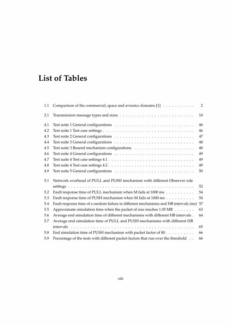
List of Tables
1.1 Comparison of the commercial, space and avionics domains [1] . . . . . . . . . . . 2
2.1 Transmission message types and sizes . . . . . . . . . . . . . . . . . . . . . . . . . . 10
4.1 Test suite 1 General configurations . . . . . . . . . . . . . . . . . . . . . . . . . . . . 464.2 Test suite 1 Test case settings . . . . . . . . . . . . . . . . . . . . . . . . . . . . . . . . 464.3 Test suite 2 General configurations . . . . . . . . . . . . . . . . . . . . . . . . . . . . 474.4 Test suite 3 General configurations . . . . . . . . . . . . . . . . . . . . . . . . . . . . 484.5 Test suite 3 Resend mechanism configurations . . . . . . . . . . . . . . . . . . . . . 484.6 Test suite 4 General configurations . . . . . . . . . . . . . . . . . . . . . . . . . . . . 494.7 Test suite 4 Test case settings 4.1 . . . . . . . . . . . . . . . . . . . . . . . . . . . . . . 494.8 Test suite 4 Test case settings 4.2 . . . . . . . . . . . . . . . . . . . . . . . . . . . . . . 494.9 Test suite 5 General configurations . . . . . . . . . . . . . . . . . . . . . . . . . . . . 50
5.1 Network overhead of PULL and PUSH mechanism with different Observer rolesettings . . . . . . . . . . . . . . . . . . . . . . . . . . . . . . . . . . . . . . . . . . . . 52
5.2 Fault response time of PULL mechanism when M fails at 1000 ms . . . . . . . . . . 545.3 Fault response time of PUSH mechanism when M fails at 1000 ms . . . . . . . . . . 545.4 Fault response time of a random failure in different mechanisms and HB intervals (ms) 575.5 Approximate simulation time when the packet of size reaches 1.05 MB . . . . . . . 635.6 Average end simulation time of different mechanisms with different HB intervals . 645.7 Average end simulation time of PULL and PUSH mechanisms with different HB
intervals . . . . . . . . . . . . . . . . . . . . . . . . . . . . . . . . . . . . . . . . . . . 655.8 End simulation time of PUSH mechanism with packet factor of 80 . . . . . . . . . . 665.9 Percentage of the tests with different packet factors that run over the threshold . . 66
xiii

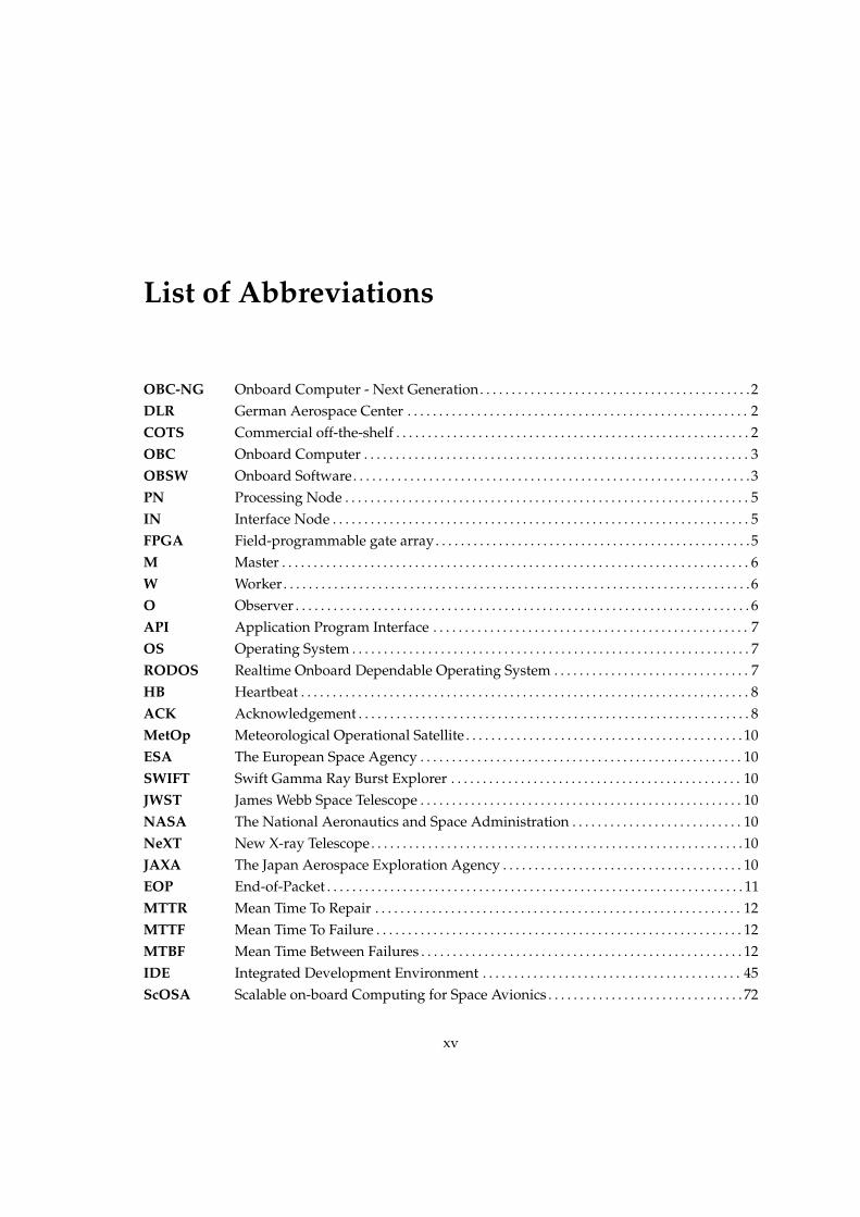
List of Abbreviations
OBC-NG Onboard Computer - Next Generation. . . . . . . . . . . . . . . . . . . . . . . . . . . . . . . . . . . . . . . . . . .2DLR German Aerospace Center . . . . . . . . . . . . . . . . . . . . . . . . . . . . . . . . . . . . . . . . . . . . . . . . . . . . . . 2COTS Commercial off-the-shelf . . . . . . . . . . . . . . . . . . . . . . . . . . . . . . . . . . . . . . . . . . . . . . . . . . . . . . . . 2OBC Onboard Computer . . . . . . . . . . . . . . . . . . . . . . . . . . . . . . . . . . . . . . . . . . . . . . . . . . . . . . . . . . . . . 3OBSW Onboard Software. . . . . . . . . . . . . . . . . . . . . . . . . . . . . . . . . . . . . . . . . . . . . . . . . . . . . . . . . . . . . . .3PN Processing Node . . . . . . . . . . . . . . . . . . . . . . . . . . . . . . . . . . . . . . . . . . . . . . . . . . . . . . . . . . . . . . . . 5IN Interface Node . . . . . . . . . . . . . . . . . . . . . . . . . . . . . . . . . . . . . . . . . . . . . . . . . . . . . . . . . . . . . . . . . . 5FPGA Field-programmable gate array. . . . . . . . . . . . . . . . . . . . . . . . . . . . . . . . . . . . . . . . . . . . . . . . . .5M Master . . . . . . . . . . . . . . . . . . . . . . . . . . . . . . . . . . . . . . . . . . . . . . . . . . . . . . . . . . . . . . . . . . . . . . . . . . 6W Worker. . . . . . . . . . . . . . . . . . . . . . . . . . . . . . . . . . . . . . . . . . . . . . . . . . . . . . . . . . . . . . . . . . . . . . . . . .6O Observer . . . . . . . . . . . . . . . . . . . . . . . . . . . . . . . . . . . . . . . . . . . . . . . . . . . . . . . . . . . . . . . . . . . . . . . . 6API Application Program Interface . . . . . . . . . . . . . . . . . . . . . . . . . . . . . . . . . . . . . . . . . . . . . . . . . . 7OS Operating System . . . . . . . . . . . . . . . . . . . . . . . . . . . . . . . . . . . . . . . . . . . . . . . . . . . . . . . . . . . . . . . 7RODOS Realtime Onboard Dependable Operating System . . . . . . . . . . . . . . . . . . . . . . . . . . . . . . . 7HB Heartbeat . . . . . . . . . . . . . . . . . . . . . . . . . . . . . . . . . . . . . . . . . . . . . . . . . . . . . . . . . . . . . . . . . . . . . . . 8ACK Acknowledgement . . . . . . . . . . . . . . . . . . . . . . . . . . . . . . . . . . . . . . . . . . . . . . . . . . . . . . . . . . . . . . 8MetOp Meteorological Operational Satellite . . . . . . . . . . . . . . . . . . . . . . . . . . . . . . . . . . . . . . . . . . . . 10ESA The European Space Agency . . . . . . . . . . . . . . . . . . . . . . . . . . . . . . . . . . . . . . . . . . . . . . . . . . . 10SWIFT Swift Gamma Ray Burst Explorer . . . . . . . . . . . . . . . . . . . . . . . . . . . . . . . . . . . . . . . . . . . . . . 10JWST James Webb Space Telescope . . . . . . . . . . . . . . . . . . . . . . . . . . . . . . . . . . . . . . . . . . . . . . . . . . . 10NASA The National Aeronautics and Space Administration . . . . . . . . . . . . . . . . . . . . . . . . . . . 10NeXT New X-ray Telescope. . . . . . . . . . . . . . . . . . . . . . . . . . . . . . . . . . . . . . . . . . . . . . . . . . . . . . . . . . .10JAXA The Japan Aerospace Exploration Agency . . . . . . . . . . . . . . . . . . . . . . . . . . . . . . . . . . . . . . 10EOP End-of-Packet . . . . . . . . . . . . . . . . . . . . . . . . . . . . . . . . . . . . . . . . . . . . . . . . . . . . . . . . . . . . . . . . . . 11MTTR Mean Time To Repair . . . . . . . . . . . . . . . . . . . . . . . . . . . . . . . . . . . . . . . . . . . . . . . . . . . . . . . . . . 12MTTF Mean Time To Failure . . . . . . . . . . . . . . . . . . . . . . . . . . . . . . . . . . . . . . . . . . . . . . . . . . . . . . . . . . 12MTBF Mean Time Between Failures . . . . . . . . . . . . . . . . . . . . . . . . . . . . . . . . . . . . . . . . . . . . . . . . . . . 12IDE Integrated Development Environment . . . . . . . . . . . . . . . . . . . . . . . . . . . . . . . . . . . . . . . . . 45ScOSA Scalable on-board Computing for Space Avionics . . . . . . . . . . . . . . . . . . . . . . . . . . . . . . . 72
xv

Chapter 1
Introduction
The goal of this chapter is to provide an introduction to the topic, and to discuss the motivations aswell as problem statement of this work. The purpose and goals are explained, along with the taskdetails. The chapter is finalized with the chapter overview.
1.1 Motivation and Problem Statement
As human explore deeper into the space, the complexity of the spacecraft design increases dra-matically. The size and the amount of collected data grow because better sensors with higherresolution are used and mission periods are getting longer. However, deep space missions have thelimitation of low telemetry bandwidths and long propagation delays between spacecraft systemand ground control [9]. The bandwidth limits the amount of data to be transmitted and thereforethe preprocessing of data before transmitting is required. Long command delay, which is causedby the communication latency, is another issue to be concerned of because todays’ space system isbecoming more autonomous and requires faster reaction time [1]. Rosetta spacecraft and its roboticcomet lander, Philae, is a good example for this requirement, since it requires onboard processingof optical data for navigation as well as for reducing and filtering images before transferring toground [10].
1
2 CHAPTER 1. INTRODUCTION
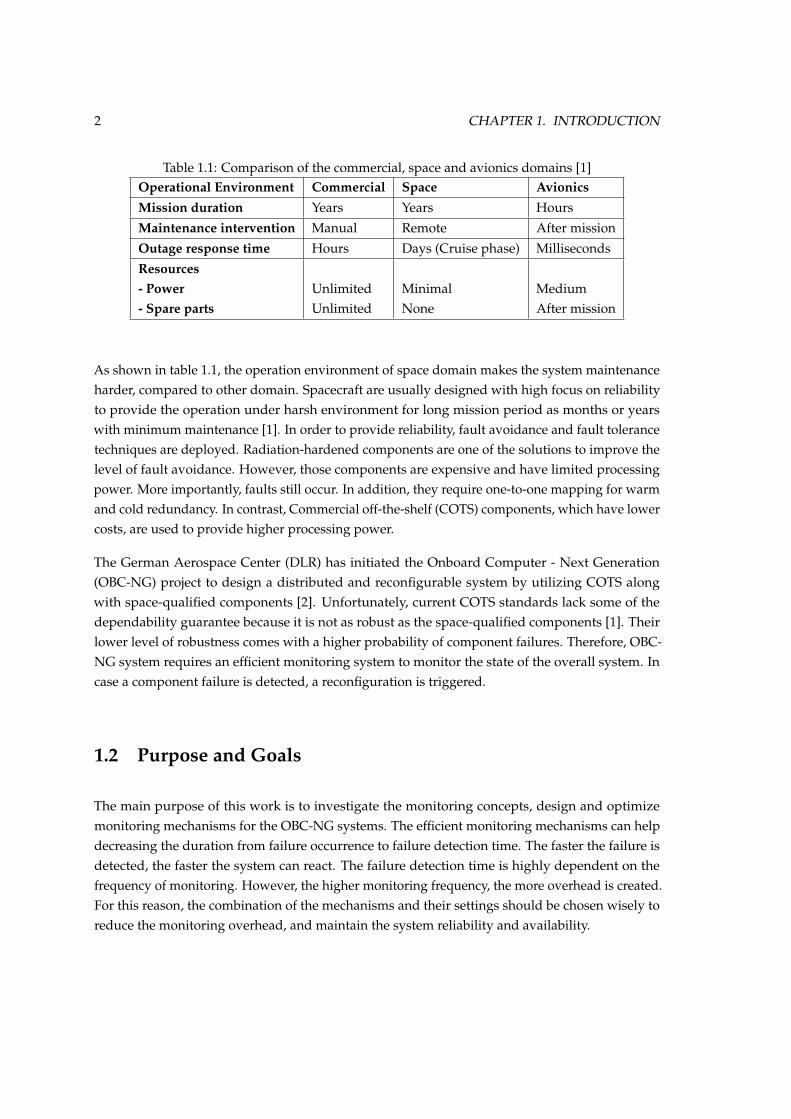
Table 1.1: Comparison of the commercial, space and avionics domains [1]Operational Environment Commercial Space AvionicsMission duration Years Years HoursMaintenance intervention Manual Remote After missionOutage response time Hours Days (Cruise phase) MillisecondsResources- Power- Spare parts
UnlimitedUnlimited
MinimalNone
MediumAfter mission
As shown in table 1.1, the operation environment of space domain makes the system maintenanceharder, compared to other domain. Spacecraft are usually designed with high focus on reliabilityto provide the operation under harsh environment for long mission period as months or yearswith minimum maintenance [1]. In order to provide reliability, fault avoidance and fault tolerancetechniques are deployed. Radiation-hardened components are one of the solutions to improve thelevel of fault avoidance. However, those components are expensive and have limited processingpower. More importantly, faults still occur. In addition, they require one-to-one mapping for warmand cold redundancy. In contrast, Commercial off-the-shelf (COTS) components, which have lowercosts, are used to provide higher processing power.
The German Aerospace Center (DLR) has initiated the Onboard Computer - Next Generation(OBC-NG) project to design a distributed and reconfigurable system by utilizing COTS alongwith space-qualified components [2]. Unfortunately, current COTS standards lack some of thedependability guarantee because it is not as robust as the space-qualified components [1]. Theirlower level of robustness comes with a higher probability of component failures. Therefore, OBC-NG system requires an efficient monitoring system to monitor the state of the overall system. Incase a component failure is detected, a reconfiguration is triggered.
1.2 Purpose and Goals
The main purpose of this work is to investigate the monitoring concepts, design and optimizemonitoring mechanisms for the OBC-NG systems. The efficient monitoring mechanisms can helpdecreasing the duration from failure occurrence to failure detection time. The faster the failure isdetected, the faster the system can react. The failure detection time is highly dependent on thefrequency of monitoring. However, the higher monitoring frequency, the more overhead is created.For this reason, the combination of the mechanisms and their settings should be chosen wisely toreduce the monitoring overhead, and maintain the system reliability and availability.
1.3. TASK 3
1.3 Task
The task is divided into four phases: Research, Design, Simulation and Implementation, as well asEvaluation Phase.
1.3.1 Research Phase
In research phase, Onboard Computer (OBC), Onboard Software (OBSW) and spacecraft systemfundamentals are investigated. The requirements of the OBC-NG system are analyzed. Variousmonitoring concepts and mechanisms, which are used in different applications of distributedsystems, are collected to analyze their advantages and disadvantages as a qualitative trade-offanalysis.
1.3.2 Design Phase
Base on the gained knowledge from the previous phase. The monitoring concepts are chosen andmodeled along with their settings. In addition, the environment settings are defined in order totest the model in the next phase.
1.3.3 Simulation and Implementation Phase
In this phase, the OBC-NG system is simulated on a discrete event simulator: OMNeT++. Themonitoring models are implemented and simulated to evaluate their efficiency and measure theircommunication overhead. The models are also tested under different scenarios to compare theirmonitoring efficiency.
1.3.4 Evaluation Phase
The test results from the previous phase are evaluated according to the specified criteria, such asmonitoring overhead and fault response time. At the end of this phase, the suitable monitoringmechanisms and their settings, e.g. monitoring frequency and number of observers needed, aredetermined in the simulation results analysis.
1.4 Chapter Overview
The structure of this report is as follows: After a brief introduction in this chapter, chapter 2provides more detailed information of distributed systems and spacecraft design and gives an

4 CHAPTER 1. INTRODUCTION
overview of monitoring. In addition, various monitoring mechanisms are investigated in therelated work section. Chapter 3 presents the monitoring requirements and the design concepts.The details about simulation and implementation are explained in chapter 4. Chapter 5 presentsthe simulation results and their evaluation. Finally, chapter 6 concludes the work and provides afuture outlook.
Chapter 2
Background
This chapter contains the basic information for the following chapters. It introduces the concepts,structure and functionality of the OBC-NG system in section 2.1. In section 2.2, the fundamentalsof the distributed systems design are explained. Afterwards, the basic concepts of monitoringare described in section 2.3. Finally, the monitoring approaches are investigated at the end of thechapter in the related work, section 2.4.
2.1 Onboard Computer Next Generation: OBC-NG
This section begins with the overview of the OBC-NG system architecture and software architecturewith the focus on the Middleware layer and its functionality and finally emphasizes its monitoringand monitoring-related functionality.
2.1.1 System Architecture
OBC-NG Nodes
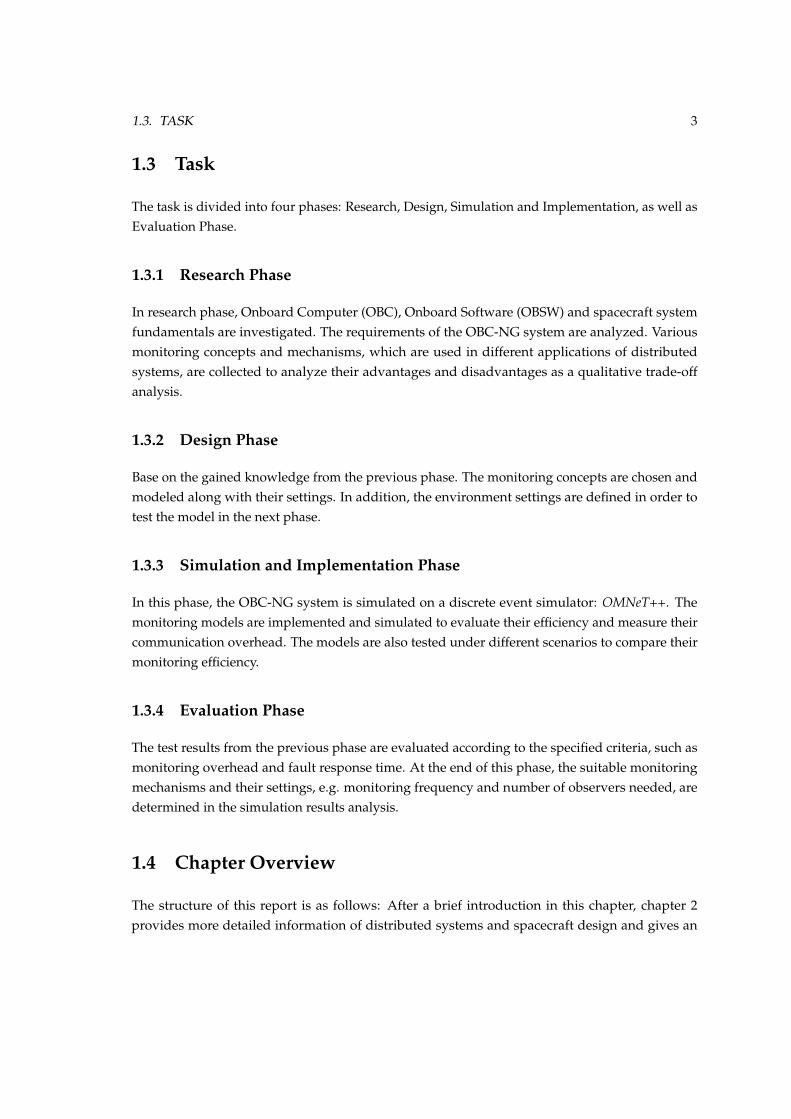
Figure 2.1 shows an example of OBC-NG system architecture with different types of nodes con-nected with point-to-point links. The first type, Processing Node (PN), provides the computingresource for processing data and managing the system. The hardware of a PN consists of MainProcessing Unit, router and optional coprocessor e.g. Field-programmable gate array (FPGA). Thesecond type is Interface Node (IN). Its hardware components consist of microcontroller, router,interfaces to periphery and mass storage. It is used to connect the PNs with the peripheries. If itconnects to mass-memory, it has the role of Storage and if it connects to sensors or actuators, it hasthe role of Interface [11].
5
6 CHAPTER 2. BACKGROUND
Figure 2.1: An example of OBC-NG system [2]
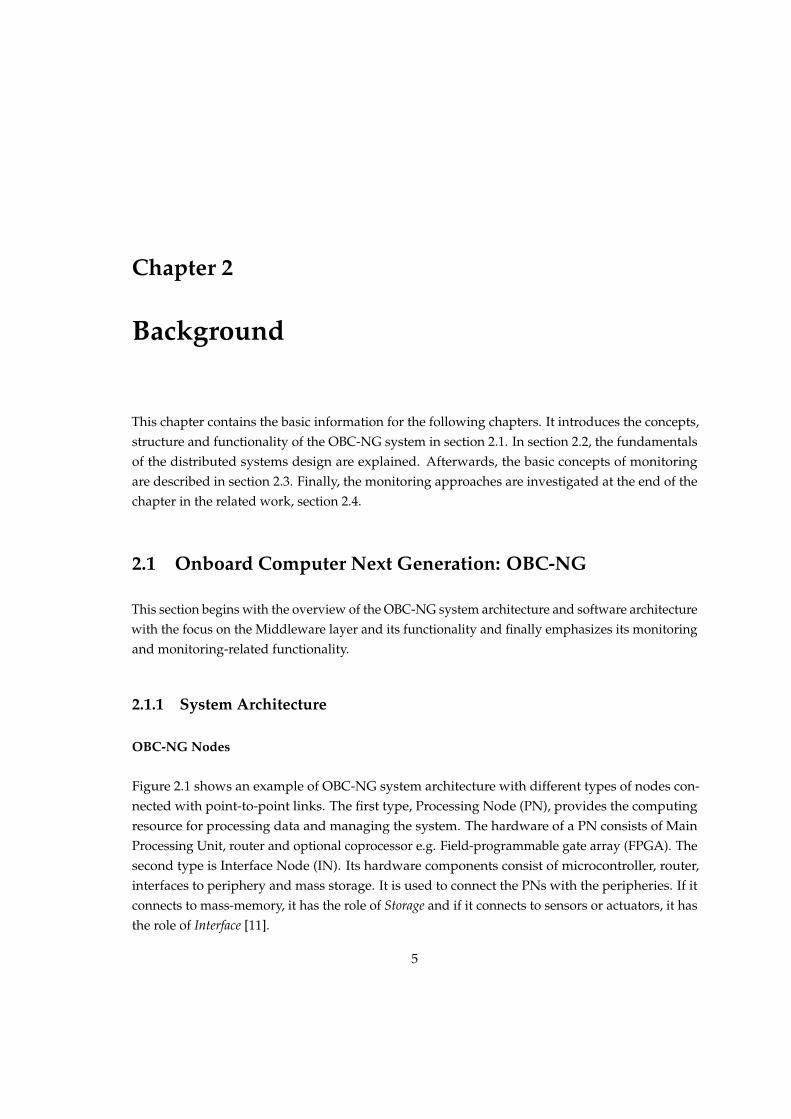
Peng et al. explained the roles of the PNs as following. The roles of the Master (M) are controllingand monitoring the other nodes and distributing the tasks. Observers (Os) have the role ofmonitoring the Master and higher priority Observer(s) as shown in figure 2.2. The PNs, whichhave no management functions of monitoring and managing the tasks, are Workers (Ws). Theyperform the data processing tasks assigned by the Master [11]. The roles can be assigned andre-assigned to the chosen nodes during system runtime because of the reconfigurable characteristicof OBC-NG nodes. Moreover, more than one role can be assigned to a single node. For example,the Master can also be assigned to perform other tasks along with the management roles. However,two management roles, i.e. Master and Observer, or two Observers, cannot be assigned on thesame node because if the node fails, the management roles will not be able to detect each other’sfailure.
Figure 2.2: Monitoring service of different types of nodes
2.1. ONBOARD COMPUTER NEXT GENERATION: OBC-NG 7
Software Architecture
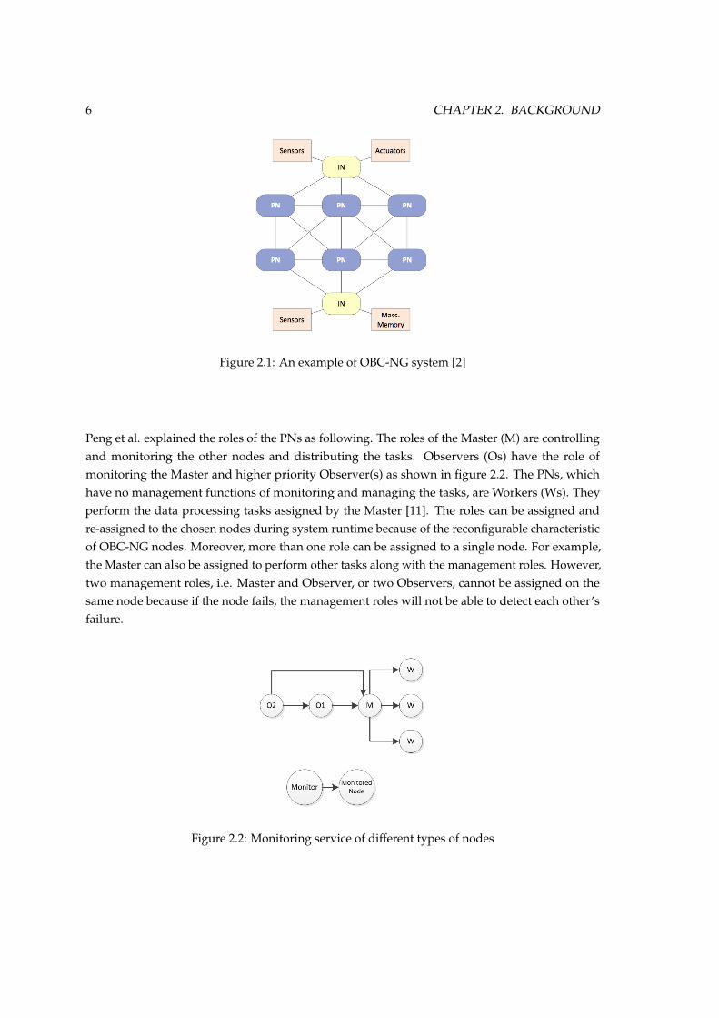
Figure 2.3 shows the OBC-NG software architecture, which is the three layers on top of hardwarelayer. Our focus is on the Middleware layer, which is between the Application layer and the OperatingSystem layer. It offers an Application Program Interface (API) for developing applications andmanagement, monitoring and reconfiguration of application tasks [2]. For the Operating System(OS), DLR has chosen two OS for OBC-NG project for different purposes; Linux for complexapplications and Realtime Onboard Dependable Operating System (RODOS) for time-criticalapplications [2].
Figure 2.3: Basic software architecture of OBC-NG [2]
2.1.2 Middleware
OBC-NG middleware consists of API, Tasking Framework, Management and Network Protocollayer as can be seen in the figure 2.4 below [2]. The API layer provides the communication serviceand passes messages to be handled by the Tasking Framework. The OBC-NG applications run astasks within the Tasking Framework. The services, which are related to the monitoring systemdesign, are monitoring and reconfiguration services in the Management layer and the communicationservices in Network protocol layer. All middleware services are provided using message-triggeredand event-triggered mechanisms [2].
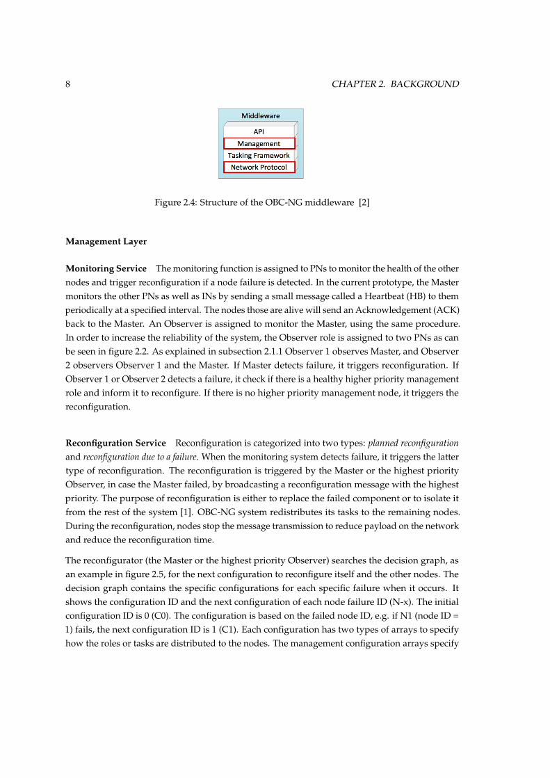
8 CHAPTER 2. BACKGROUND
Figure 2.4: Structure of the OBC-NG middleware [2]
Management Layer
Monitoring Service The monitoring function is assigned to PNs to monitor the health of the othernodes and trigger reconfiguration if a node failure is detected. In the current prototype, the Mastermonitors the other PNs as well as INs by sending a small message called a Heartbeat (HB) to themperiodically at a specified interval. The nodes those are alive will send an Acknowledgement (ACK)back to the Master. An Observer is assigned to monitor the Master, using the same procedure.In order to increase the reliability of the system, the Observer role is assigned to two PNs as canbe seen in figure 2.2. As explained in subsection 2.1.1 Observer 1 observes Master, and Observer2 observers Observer 1 and the Master. If Master detects failure, it triggers reconfiguration. IfObserver 1 or Observer 2 detects a failure, it check if there is a healthy higher priority managementrole and inform it to reconfigure. If there is no higher priority management node, it triggers thereconfiguration.
Reconfiguration Service Reconfiguration is categorized into two types: planned reconfigurationand reconfiguration due to a failure. When the monitoring system detects failure, it triggers the lattertype of reconfiguration. The reconfiguration is triggered by the Master or the highest priorityObserver, in case the Master failed, by broadcasting a reconfiguration message with the highestpriority. The purpose of reconfiguration is either to replace the failed component or to isolate itfrom the rest of the system [1]. OBC-NG system redistributes its tasks to the remaining nodes.During the reconfiguration, nodes stop the message transmission to reduce payload on the networkand reduce the reconfiguration time.
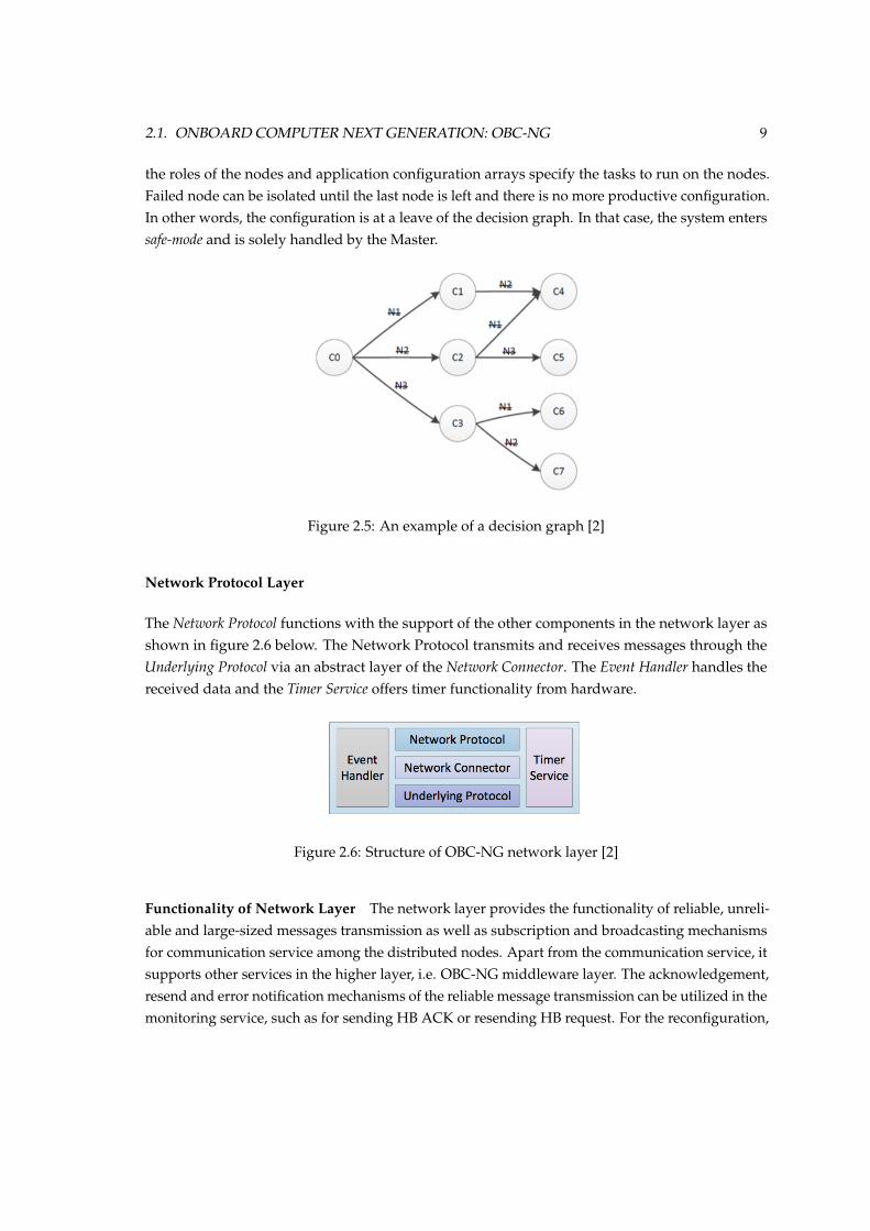
The reconfigurator (the Master or the highest priority Observer) searches the decision graph, asan example in figure 2.5, for the next configuration to reconfigure itself and the other nodes. Thedecision graph contains the specific configurations for each specific failure when it occurs. Itshows the configuration ID and the next configuration of each node failure ID (N-x). The initialconfiguration ID is 0 (C0). The configuration is based on the failed node ID, e.g. if N1 (node ID =1) fails, the next configuration ID is 1 (C1). Each configuration has two types of arrays to specifyhow the roles or tasks are distributed to the nodes. The management configuration arrays specify
2.1. ONBOARD COMPUTER NEXT GENERATION: OBC-NG 9
the roles of the nodes and application configuration arrays specify the tasks to run on the nodes.Failed node can be isolated until the last node is left and there is no more productive configuration.In other words, the configuration is at a leave of the decision graph. In that case, the system enterssafe-mode and is solely handled by the Master.
Figure 2.5: An example of a decision graph [2]
Network Protocol Layer
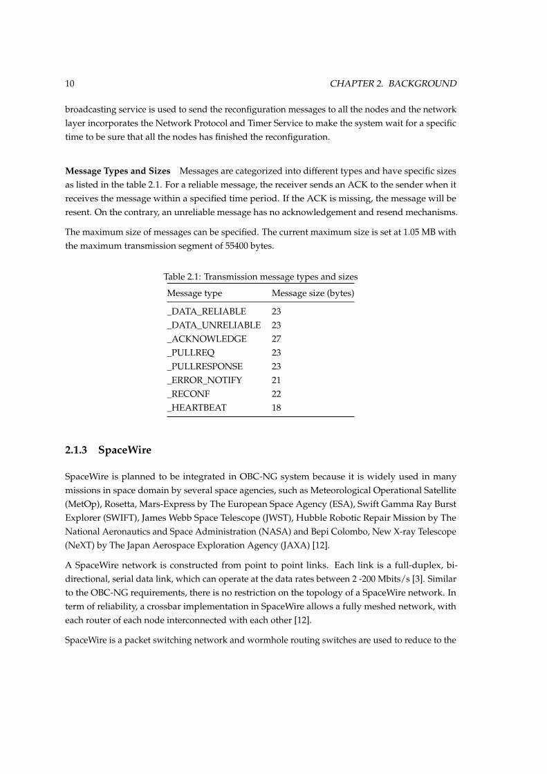
The Network Protocol functions with the support of the other components in the network layer asshown in figure 2.6 below. The Network Protocol transmits and receives messages through theUnderlying Protocol via an abstract layer of the Network Connector. The Event Handler handles thereceived data and the Timer Service offers timer functionality from hardware.
Figure 2.6: Structure of OBC-NG network layer [2]
Functionality of Network Layer The network layer provides the functionality of reliable, unreli-able and large-sized messages transmission as well as subscription and broadcasting mechanismsfor communication service among the distributed nodes. Apart from the communication service, itsupports other services in the higher layer, i.e. OBC-NG middleware layer. The acknowledgement,resend and error notification mechanisms of the reliable message transmission can be utilized in themonitoring service, such as for sending HB ACK or resending HB request. For the reconfiguration,
10 CHAPTER 2. BACKGROUND
broadcasting service is used to send the reconfiguration messages to all the nodes and the networklayer incorporates the Network Protocol and Timer Service to make the system wait for a specifictime to be sure that all the nodes has finished the reconfiguration.
Message Types and Sizes Messages are categorized into different types and have specific sizesas listed in the table 2.1. For a reliable message, the receiver sends an ACK to the sender when itreceives the message within a specified time period. If the ACK is missing, the message will beresent. On the contrary, an unreliable message has no acknowledgement and resend mechanisms.
The maximum size of messages can be specified. The current maximum size is set at 1.05 MB withthe maximum transmission segment of 55400 bytes.
Table 2.1: Transmission message types and sizes
Message type Message size (bytes)
_DATA_RELIABLE 23_DATA_UNRELIABLE 23_ACKNOWLEDGE 27_PULLREQ 23_PULLRESPONSE 23_ERROR_NOTIFY 21_RECONF 22_HEARTBEAT 18
2.1.3 SpaceWire
SpaceWire is planned to be integrated in OBC-NG system because it is widely used in manymissions in space domain by several space agencies, such as Meteorological Operational Satellite(MetOp), Rosetta, Mars-Express by The European Space Agency (ESA), Swift Gamma Ray BurstExplorer (SWIFT), James Webb Space Telescope (JWST), Hubble Robotic Repair Mission by TheNational Aeronautics and Space Administration (NASA) and Bepi Colombo, New X-ray Telescope(NeXT) by The Japan Aerospace Exploration Agency (JAXA) [12].
A SpaceWire network is constructed from point to point links. Each link is a full-duplex, bi-directional, serial data link, which can operate at the data rates between 2 -200 Mbits/s [3]. Similarto the OBC-NG requirements, there is no restriction on the topology of a SpaceWire network. Interm of reliability, a crossbar implementation in SpaceWire allows a fully meshed network, witheach router of each node interconnected with each other [12].
SpaceWire is a packet switching network and wormhole routing switches are used to reduce to the
2.2. DISTRIBUTED SYSTEM DESIGN 11
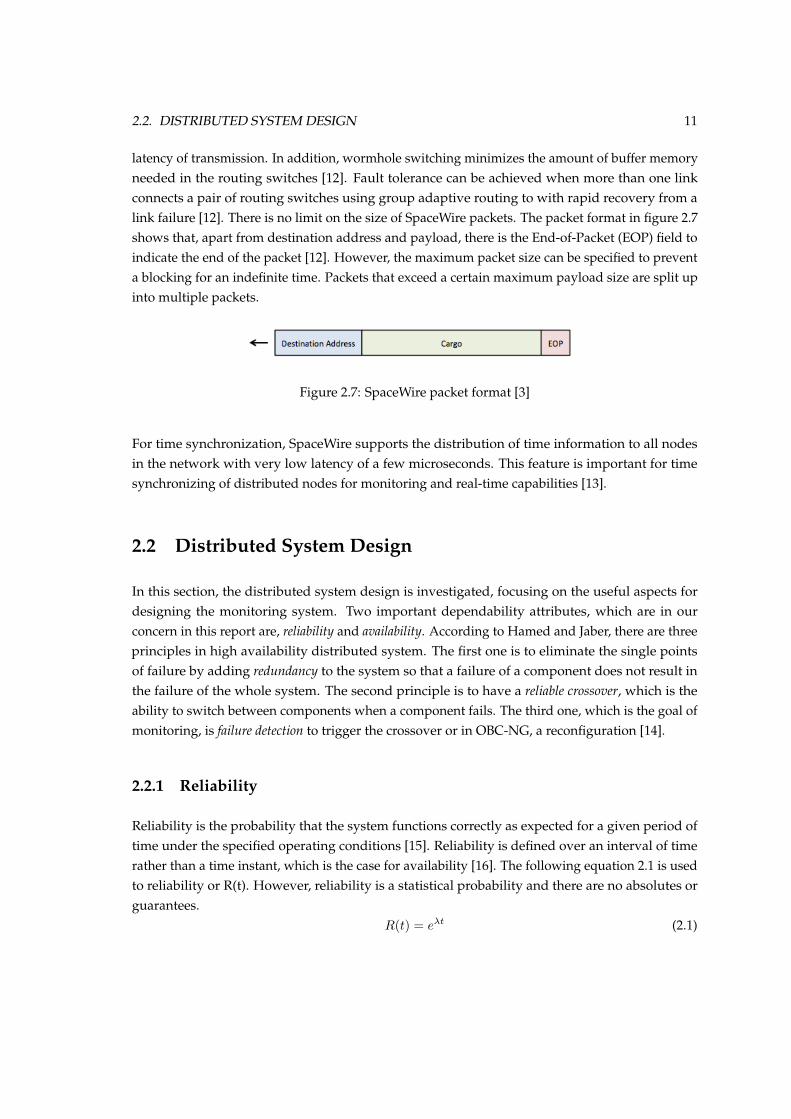
latency of transmission. In addition, wormhole switching minimizes the amount of buffer memoryneeded in the routing switches [12]. Fault tolerance can be achieved when more than one linkconnects a pair of routing switches using group adaptive routing to with rapid recovery from alink failure [12]. There is no limit on the size of SpaceWire packets. The packet format in figure 2.7shows that, apart from destination address and payload, there is the End-of-Packet (EOP) field toindicate the end of the packet [12]. However, the maximum packet size can be specified to preventa blocking for an indefinite time. Packets that exceed a certain maximum payload size are split upinto multiple packets.
Figure 2.7: SpaceWire packet format [3]
For time synchronization, SpaceWire supports the distribution of time information to all nodesin the network with very low latency of a few microseconds. This feature is important for timesynchronizing of distributed nodes for monitoring and real-time capabilities [13].
2.2 Distributed System Design
In this section, the distributed system design is investigated, focusing on the useful aspects fordesigning the monitoring system. Two important dependability attributes, which are in ourconcern in this report are, reliability and availability. According to Hamed and Jaber, there are threeprinciples in high availability distributed system. The first one is to eliminate the single pointsof failure by adding redundancy to the system so that a failure of a component does not result inthe failure of the whole system. The second principle is to have a reliable crossover, which is theability to switch between components when a component fails. The third one, which is the goal ofmonitoring, is failure detection to trigger the crossover or in OBC-NG, a reconfiguration [14].
2.2.1 Reliability
Reliability is the probability that the system functions correctly as expected for a given period oftime under the specified operating conditions [15]. Reliability is defined over an interval of timerather than a time instant, which is the case for availability [16]. The following equation 2.1 is usedto reliability or R(t). However, reliability is a statistical probability and there are no absolutes orguarantees.
R(t) = e�t (2.1)
12 CHAPTER 2. BACKGROUND
t is the mission time, or the time the system must execute without an outage� is the constant failure rate over time (failures/hour)
2.2.2 Availability
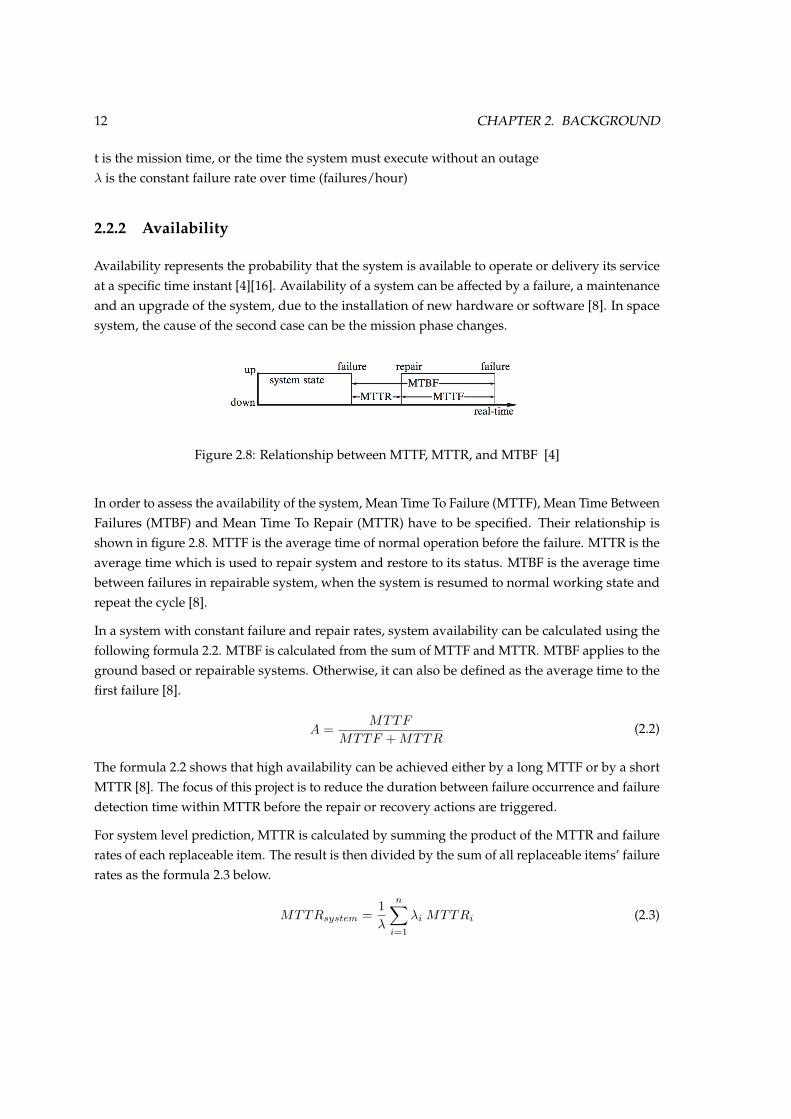
Availability represents the probability that the system is available to operate or delivery its serviceat a specific time instant [4][16]. Availability of a system can be affected by a failure, a maintenanceand an upgrade of the system, due to the installation of new hardware or software [8]. In spacesystem, the cause of the second case can be the mission phase changes.
Figure 2.8: Relationship between MTTF, MTTR, and MTBF [4]
In order to assess the availability of the system, Mean Time To Failure (MTTF), Mean Time BetweenFailures (MTBF) and Mean Time To Repair (MTTR) have to be specified. Their relationship isshown in figure 2.8. MTTF is the average time of normal operation before the failure. MTTR is theaverage time which is used to repair system and restore to its status. MTBF is the average timebetween failures in repairable system, when the system is resumed to normal working state andrepeat the cycle [8].
In a system with constant failure and repair rates, system availability can be calculated using thefollowing formula 2.2. MTBF is calculated from the sum of MTTF and MTTR. MTBF applies to theground based or repairable systems. Otherwise, it can also be defined as the average time to thefirst failure [8].
A =MTTF
MTTF +MTTR(2.2)
The formula 2.2 shows that high availability can be achieved either by a long MTTF or by a shortMTTR [8]. The focus of this project is to reduce the duration between failure occurrence and failuredetection time within MTTR before the repair or recovery actions are triggered.
For system level prediction, MTTR is calculated by summing the product of the MTTR and failurerates of each replaceable item. The result is then divided by the sum of all replaceable items’ failurerates as the formula 2.3 below.
MTTRsystem =1
�
nX
i=1
�i MTTRi (2.3)
2.2. DISTRIBUTED SYSTEM DESIGN 13
� is the constant failure rate over time (failures/hour)�i is the constant failure rate over time of the ith item to be repaired (failures/hour)
� =nX
i=1
�i (2.4)
2.2.3 Redundancy
Redundancy is duplication of components or repetition of operations to provide alternativefunctional channels in case of failure [17]. It can be specified into structural redundancy, which isreferred as a hardware method [16] and functional redundancy, which is achieved by a softwaremethod. Functional redundancy is a system design and operations characteristic that allowsthe system to respond to component failures in a way that it is sufficient to meet the missionrequirements [15].
Azambuja et al. categorized redundancy into time and space redundancy. Time redundancy uses theoutputs generated by the same component(s) by comparing the values at two different momentsin time, separated by a fixed delay [18]. For Space redundancy, the outputs generated by differentcomponents at the same time are compared. If there is a mismatch, the failure is detected [19].
For the monitoring design, the redundancy concept will be used to determine the number ofObservers. Hamed and Jaber explained about redundancy simulation in their work with N-xcriteria. N is the total number of components in the system. x represents the number of componentsused to stress the system. The (N-1) criteria means the model is stressed by evaluating performancewith all possible combinations where one machine fails. The (N-2) criteria means the modelis stressed by evaluating performance with all possible combinations where two machines failsimultaneously [14].
2.2.4 Threats
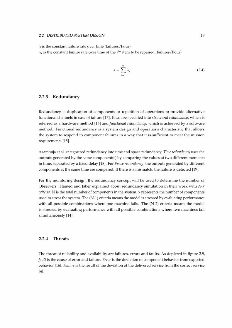
The threat of reliability and availability are failures, errors and faults. As depicted in figure 2.9,fault is the cause of error and failure. Error is the deviation of component behavior from expectedbehavior [16]. Failure is the result of the deviation of the delivered service from the correct service[4].
14 CHAPTER 2. BACKGROUND
Figure 2.9: Failure, Error and Fault [4]
Failure Rate
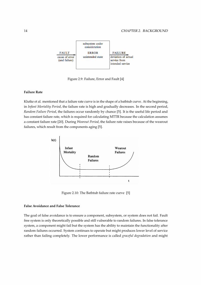
Klutke et al. mentioned that a failure rate curve is in the shape of a bathtub curve. At the beginning,in Infant Mortality Period, the failure rate is high and gradually decreases. In the second period,Random Failure Period, the failures occur randomly by chance [5]. It is the useful life period andhas constant failure rate, which is required for calculating MTTR because the calculation assumesa constant failure rate [20]. During Wearout Period, the failure rate raises because of the wearoutfailures, which result from the components aging [5].
Figure 2.10: The Bathtub failure rate curve [5]
False Avoidance and False Tolerance
The goal of false avoidance is to ensure a component, subsystem, or system does not fail. Faultfree system is only theoretically possible and still vulnerable to random failures. In false tolerancesystem, a component might fail but the system has the ability to maintain the functionality afterrandom failures occurred. System continues to operate but might produces lower level of servicerather than failing completely. The lower performance is called graceful degradation and might
2.3. MONITORING 15
be because some failed components are switched off in reconfiguration process [1]. The mostimportant method supporting fault tolerance is redundancy.
2.2.5 Design Validation: Fault Injection
Fault injection technique is used to evaluate the efficiency of error detection techniques and assessthe fault tolerant systems. Its goal is validate the design with respect to reliability [16]. This reportfocuses on the simulation-based fault injection. Fault injection at random time on random nodewill be simulated to represent the random failure in the useful period of the failure rate curve.
2.3 Monitoring
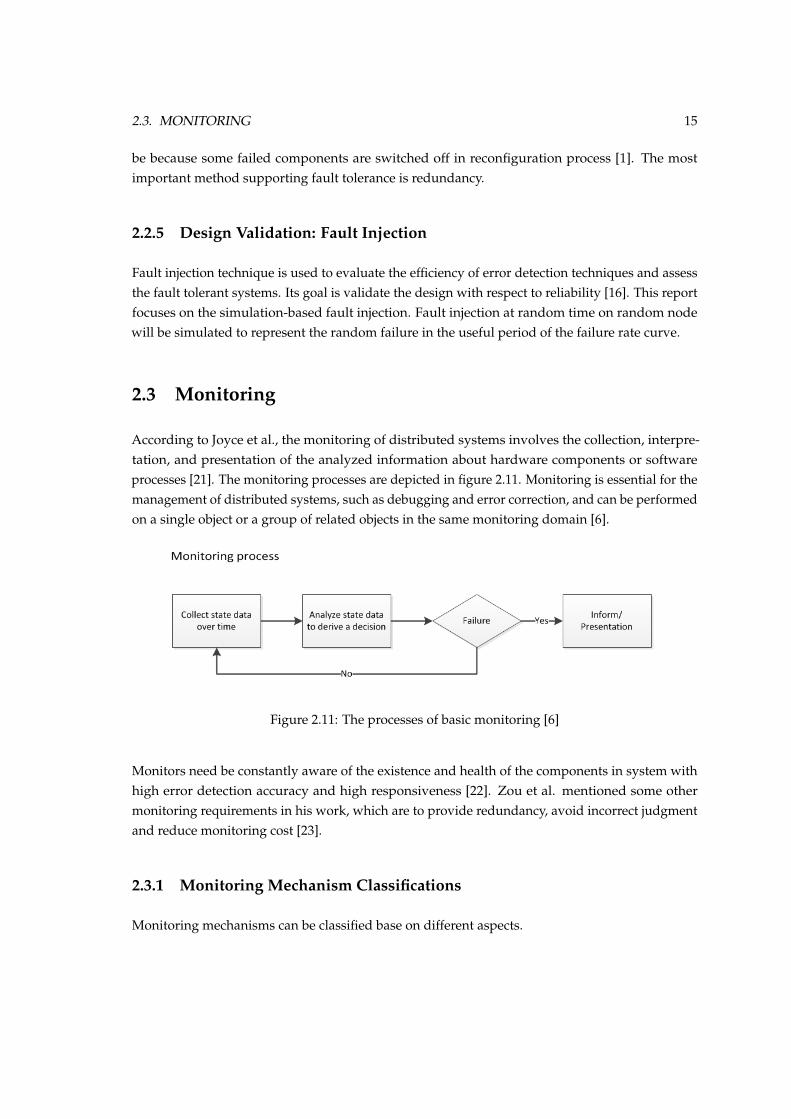
According to Joyce et al., the monitoring of distributed systems involves the collection, interpre-tation, and presentation of the analyzed information about hardware components or softwareprocesses [21]. The monitoring processes are depicted in figure 2.11. Monitoring is essential for themanagement of distributed systems, such as debugging and error correction, and can be performedon a single object or a group of related objects in the same monitoring domain [6].
Figure 2.11: The processes of basic monitoring [6]
Monitors need be constantly aware of the existence and health of the components in system withhigh error detection accuracy and high responsiveness [22]. Zou et al. mentioned some othermonitoring requirements in his work, which are to provide redundancy, avoid incorrect judgmentand reduce monitoring cost [23].
2.3.1 Monitoring Mechanism Classifications
Monitoring mechanisms can be classified base on different aspects.
16 CHAPTER 2. BACKGROUND
Base on how a failure is detected, monitoring mechanisms can be categorized into two categories.In active monitoring, sensors continuously send a small-sized message to show that it is aliveto its control center. In this case, it is an implicit detection because the control centers sense thecommunication from the sensors and a missing alive-message after a predetermined timeoutimplies failure. The control center has an overview of the health its sensors. In passive monitoring,control center expects no message from sensors unless there is something wrong. This is an explicitdetection, in which the monitored sensors are able to detect failures and send an alarm to controlcenter [22].
Base on which kind of monitoring information is obtained, monitoring can be classified intotime-driven monitoring and event-driven monitoring. Time-driven monitoring is based on acquiringperiodic health status information to provide an instantaneous view of the behavior of an object ora group of objects. The status of an object has a duration in time. For example, a node is alive for aspecific duration. Event-driven monitoring is based on obtaining information about the occurrenceof specific events, which provide a dynamic view of system activity, as only information about thechanges in the system are collected. An event is an atomic entity that reflects a change in the statusof an object and occurs instantaneously. For example, message sent, counter reach threshold [6].
Alternatively, monitoring mechanisms can be categorized base on error detection domain. In theDesign Principles for Distributed Embedded Applications by Hermann Kopetz, he explained thata real-time operating system must support error detection both temporal domain and value domain[4]. One of the methods to achieve these requirements is to use the watchdogs. Temporal domainis used to detect the failure of fail-silent nodes. These nodes have self-checking mechanism andeither function correctly or stop functioning and produce no results after they detect an internalfailure. [24]. A standard technique is the provision of a watchdog signal (heartbeat) that must beperiodically produced by the operating system of the node. If the node has access to the globaltime, the watchdog signal should be produced periodically at known absolute points in time. Anoutside observer can detect the failure of the node as soon as the watchdog signal disappears. Incontrast to temporal domain, for the value domain error detection, challenge-response protocol isexecuted by the error detector node. It provides an input pattern to the node and expects a definedresponse pattern within a specified time interval. The functional units required for computingthe response are checked and if the response pattern deviates from the expected result, an error isdetected.
A failure in the system can be detected at different levels of granularity. The current OBC-NGimplementation it is on node level. When a heartbeat of a node is missing, all the tasks are migratedto other nodes [2]. Theoretically, the detection could be done in a finer grained level, i.e., task levelor subnode level such as FPGA, embedded GPU. When there is a failure, all the tasks will not bemigrated to new node but only the specific task will be moved. Consequently, fewer tasks will beinterrupted and less bandwidth will be needed.
2.3. MONITORING 17
2.3.2 Fundamental Problems of Distributed System Monitoring
There are a number of fundamental problems associate with the monitoring of distributed systems.The efficiency of the system can be affected by monitoring system and vice versa.
The effects of overall system on monitoring system
As stated by Mansouri and Sloman, in distributed system, it is difficult to obtain a global view ofall the system components because of the transmission delay. The transferred monitoring messagesfrom source may already become out of date when it arrives its destination. Moreover, in themonitoring system that the sequence of information is important, time synchronization to providethe mean of determining the ordering is necessary [6].
Another issue they mentioned is, the amount of monitoring information generated in a large systemcan overburden the monitor and therefore, filtering and processing of monitoring information isnecessary. Moreover, as the monitoring system shares the resource with the observed system, ifthey compete for the resources, the monitoring behavior may alter and affects monitoring result[6].
The effects of monitoring system on overall system
The monitoring system could affect the overall system because of the resource sharing as well.Monitoring creates overhead and also requires processing power, communication bandwidth andmemory. It increases the application’s executing, workload on the Master and Observer nodes.Thus, excessive monitoring leads affects system performance [6].
In Wan et al.’s study about heartbeat cycle effect on the high availability performance dual-controller RAID system, the system contains main and passive controller. An unsuitable heartbeatcycle leads to wrong fault interpretation of controller status and wrong takeover. They mentionedthat, if the heartbeat cycle is relative short if read and write request is still in the wait queue ofthe master controller, the system interpret that main controller has failed. The master control willstart the takeover procedures and transfer request to passive controller. This transfer process takestime and greatly increases the system response time to the request. The delayed heartbeat leads towrong fault takeover when the system works normally. In addition, the frequency of heartbeatcycle adjustment should also be in consideration when design because it is proved in their workthat the frequent changes of heartbeat cycle results could affect the performance of monitoredsystem [8].
18 CHAPTER 2. BACKGROUND
2.4 Related Work
Several monitoring techniques from the previous subsection implement the heartbeat monitoringand watchdog mechanism. Heartbeat is categorized as an active and implicit monitoring becausethe monitoring messages are sent and sensed continuously and the missing of the messages impliesfailure. The advantages of heartbeat mechanism are, it only needs to maintain few states, lowmanagement is required and overhead on the system is low [22]. Zou et al. have categorizedheartbeat monitoring into traditional and hybrid heartbeat monitoring.
2.4.1 Traditional Heartbeat Monitoring
In traditional heartbeat monitoring, the heartbeat monitor adopts a model which could be PULLor PUSH models depending on different status realization patterns and which component initiatesthe monitoring message [23][25].
PULL model
Rachuri et al. explained that PULL has the concept of querying. The monitor node queries forthe required information on need basis. This is the advantage of PULL because it can be used torequest a specific data at anytime. However, if the query rate is depending on the rate of eventoccurrences because the mechanism is not efficient when query rate is low and event occurrence ishigh [26].
In term of failure detection, detection nodes in PULL model send request message to detected node.After detected nodes receive the message, they passively send response message back. Therefore,there are two way of transmission and with the same monitoring rate, the communication cost ishigher monitoring model with one way communication [23].
In summary, PULL model can be implemented in monitoring system on need basis or periodically.The current monitoring system design of OBC-NG uses PULL model for periodically monitoringnode’s health status.
PUSH model
PUSH model has the concept of continuous collection and is useful in the system where continuoussensing is required. In monitoring system, monitored node periodically sending its status tothe monitor [23]. It needs only half of the amount of messages for equivalent failure detectionefficiency because it is pushing one way [25]. However, the period and data to be sent have to bepredetermined. Therefore, it cannot be used to request specific information.
2.4. RELATED WORK 19
2.4.2 Hybrid Heartbeat Monitoring
PUSH-PULL Hybrid model
In hybrid heartbeat monitoring, the advantages of the two models can be combined. PUSH modelhas high consistency but lower efficiency, while PULL model has lower consistency but higherefficiency (if PULL model is used on need basis). The switch between PUSH and PULL styles canbe according to user requirements and resource status [27].
Zuo et al. combines these two by setting the period of PULL higher than PUSH. If the monitorreceives PUSH heartbeat messages within the specific period, the timer gets into next period.Otherwise, monitor activates the timer and adopts PULL model to detect the monitored node if itis invalid or not. If the monitor does not receive PULL response in time, the module is judged asinvalid [23].
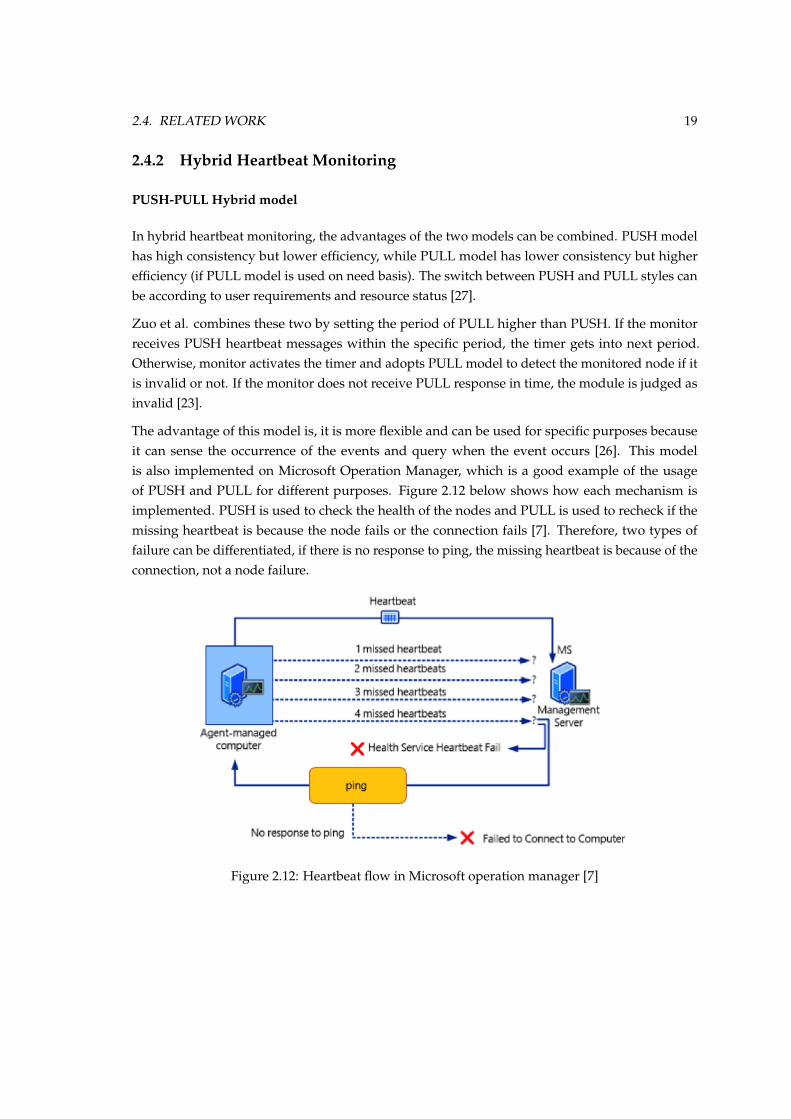
The advantage of this model is, it is more flexible and can be used for specific purposes becauseit can sense the occurrence of the events and query when the event occurs [26]. This modelis also implemented on Microsoft Operation Manager, which is a good example of the usageof PUSH and PULL for different purposes. Figure 2.12 below shows how each mechanism isimplemented. PUSH is used to check the health of the nodes and PULL is used to recheck if themissing heartbeat is because the node fails or the connection fails [7]. Therefore, two types offailure can be differentiated, if there is no response to ping, the missing heartbeat is because of theconnection, not a node failure.
Figure 2.12: Heartbeat flow in Microsoft operation manager [7]
20 CHAPTER 2. BACKGROUND
In summary, PUSH-PULL hybrid mechanism can be used for different purposes. First PUSH isused to periodically sending heartbeat to the monitor and detecting failure. When a failure isdetected, PULL can be used after a missing push heartbeat is detected for retrieving diagnosticinformation, such as request the state from specific node, or check the network connection. PULLcan also be used in the resend mechanism for requesting heartbeat to confirm the invalidity orfailure of the node.
PULL-PUSH Hybrid model
On the other hand, Zhao also mentioned PULL-PUSH hybrid model, where both consumers andsuppliers are passive. There is an event channel, which actively requests from the suppliers andpasses the response to the consumers. This model gives the channel more control on how tocoordinate the components because PULL and PUSH can be executed with various frequencies oneach component [28].
Summary of Monitoring Models
In summary, PULL mechanisms have two ways of communications, which increase networkoverhead if the querying frequency is high. Therefore, PULL is more suitable for querying data onneed basis as it can be used to request a specific data at anytime.
In contrast, PUSH is useful when continuous sensing is required but the data sent is predeterminedand fixed. It is suitable for checking the health status of the nodes since the message sent can bepredetermined as heartbeat without any system details.
PUSH-PULL hybrid model can be used to differentiate two types of failures, such as node failureand network failure. In addition, it can be used to confirm the invalidity or failure of the node.PULL-PUSH hybrid model has passive consumers and producers but the model requires an eventchannel.
2.4.3 Dynamic Heartbeat
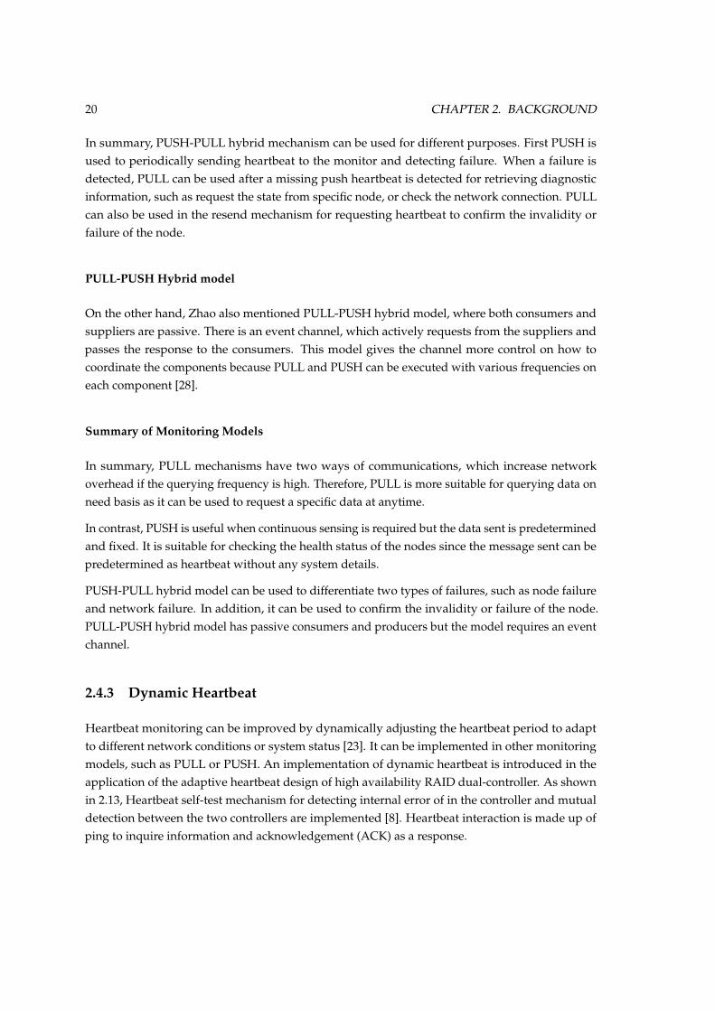
Heartbeat monitoring can be improved by dynamically adjusting the heartbeat period to adaptto different network conditions or system status [23]. It can be implemented in other monitoringmodels, such as PULL or PUSH. An implementation of dynamic heartbeat is introduced in theapplication of the adaptive heartbeat design of high availability RAID dual-controller. As shownin 2.13, Heartbeat self-test mechanism for detecting internal error of in the controller and mutualdetection between the two controllers are implemented [8]. Heartbeat interaction is made up ofping to inquire information and acknowledgement (ACK) as a response.
2.4. RELATED WORK 21
Figure 2.13: Heartbeat self-test and mutual detection [8]
For dynamic heartbeat, the mechanism called Grade-Heartbeat is implemented to allow the controllerto adapt its heartbeat interval using real-time monitoring module to monitor the read and writerequests frequency. Heartbeat interval is set dynamically according to the previous 20 requestsinterval time. Their experiment also shows that frequent changes in heartbeat interval result in thedecline of overall system performance [8].

Chapter 3
Design of OBC-NG Monitoring
This chapter is divided into three sections. Section 3.1 presents the OBC-NG monitoring require-ments. The monitoring concepts from the related work are analyzed in section 3.2. Finally, themechanism settings are listed and explained in section 3.3.
3.1 OBC-NG Monitoring Requirements
General monitoring requirements and fundamental problems of distributed system monitoringare considered along with the OBC-NG’s specific requirements and combined into the OBC-NG monitoring system requirements. These requirements are used to specify the performanceindicators in the next chapter.
3.1.1 Reliability and Redundancy in Monitoring System
For the reliability, OBC-NG system requires at least one node to always be responsive to groundcommand at all times. Therefore, we need to make sure that there is always a node assigned as aMaster in the system. In the system with only one Observer, if the Master fails and the Observerfails later before the detection, the Master’s failure will never be discovered and reconfigurationwill never be triggered. Consequently, no node has the Master role and the remaining Workernodes in the system are not monitored. In contrast, if there are two Observers and one of theObservers fails at the same time as Master, the failure will be detected by the other Observer andreconfiguration will be triggered. Therefore, redundancy is required to provide the reliability.
23
24 CHAPTER 3. DESIGN OF OBC-NG MONITORING
3.1.2 Availability and MTTR
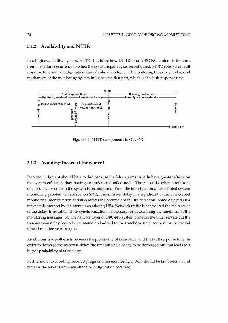
In a high availability system, MTTR should be low. MTTR of an OBC-NG system is the timefrom the failure occurrence to when the system repaired, i.e. reconfigured. MTTR consists of faultresponse time and reconfiguration time. As shown in figure 3.1, monitoring frequency and resendmechanism of the monitoring system influence the first part, which is the fault response time.
Figure 3.1: MTTR components in OBC-NG
3.1.3 Avoiding Incorrect Judgement
Incorrect judgment should be avoided because the false alarms usually have greater effects onthe system efficiency than having an undetected failed node. The reason is, when a failure isdetected, every node in the system is reconfigured. From the investigation of distributed systemmonitoring problems in subsection 2.3.2, transmission delay is a significant cause of incorrectmonitoring interpretation and also affects the accuracy of failure detection. Some delayed HBsmaybe misinterpret by the monitor as missing HBs. Network traffic is considered the main causeof the delay. In addition, clock synchronization is necessary for determining the timeliness of themonitoring messages [6]. The network layer of OBC-NG system provides the timer service but thetransmission delay has to be estimated and added to the watchdog timer to monitor the arrivaltime of monitoring messages.
An obvious trade-off exists between the probability of false alarm and the fault response time. Inorder to decrease the response delay, the timeout value needs to be decreased but that leads to ahigher probability of false alarm.
Furthermore, to avoiding incorrect judgment, the monitoring system should be fault tolerant andremains the level of accuracy after a reconfiguration occurred.
3.2. MONITORING MECHANISMS CONCEPTS 25
3.1.4 Reducing Monitoring Cost
The monitoring system should not create too much overhead that it affects the efficiency of otherapplications in the system. The number and size of monitoring messages and bandwidth usageshould be measured and compared with the overall bandwidth. The smaller the monitoringmessages, the less data has to be processed. Consequently, the CPU time and the memoryconsumption are reduced.
3.2 Monitoring Mechanisms Concepts
This section introduces the currently implemented monitoring mechanism and the other alterna-tives collected from section 2.4. The PULL, PUSH and PUSH-PULL hybrid models are analyzedwith the same monitoring roles of Master and Observers as the currently implemented model.PULL is chosen because it is used in the current monitoring system of OBC-NG. PUSH is chosenbecause it is suitable for continuous sensing, which is required for nodes’ health status monitoring.PUSH-PULL is chosen to utilize PUSH for monitoring and PULL for requesting PULL HB whena PUSH HB is missing. On the other hand, for PULL-PUSH mechanism is not chosen because itrequires an event channel and therefore, it is not suitable for point-to-point topology of OBC-NG.In addition, if PULL response is missing, PUSH cannot be used for requesting a HB in resendingmechanism.
The OBC-NG system has a Master serving as the monitor of the other nodes and two Observers asthe monitors of the Master, as mentioned in the monitoring service subsection. In this section, theMaster or an Observer is referred to as a monitor.
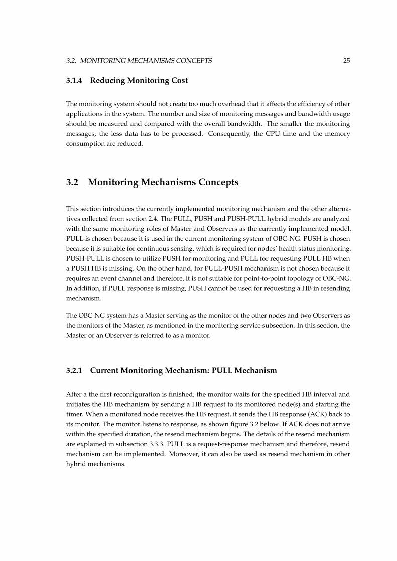
3.2.1 Current Monitoring Mechanism: PULL Mechanism
After a the first reconfiguration is finished, the monitor waits for the specified HB interval andinitiates the HB mechanism by sending a HB request to its monitored node(s) and starting thetimer. When a monitored node receives the HB request, it sends the HB response (ACK) back toits monitor. The monitor listens to response, as shown figure 3.2 below. If ACK does not arrivewithin the specified duration, the resend mechanism begins. The details of the resend mechanismare explained in subsection 3.3.3. PULL is a request-response mechanism and therefore, resendmechanism can be implemented. Moreover, it can also be used as resend mechanism in otherhybrid mechanisms.
26 CHAPTER 3. DESIGN OF OBC-NG MONITORING
Figure 3.2: Heartbeat flows in PULL mechanism
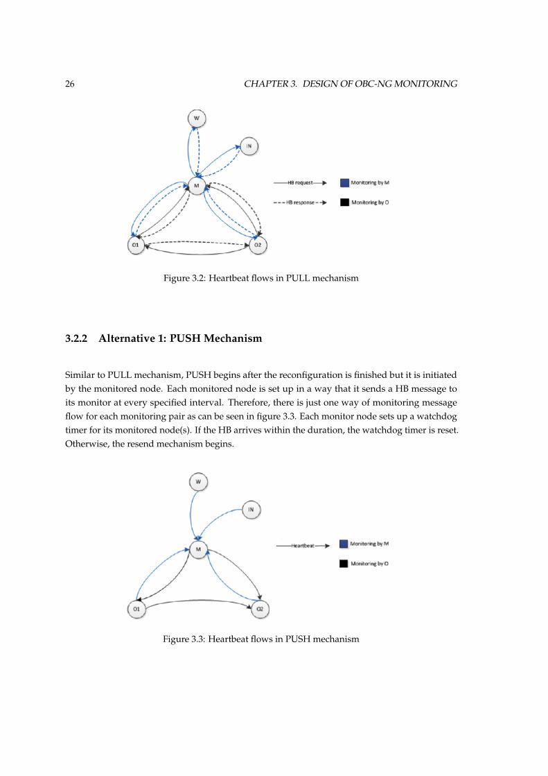
3.2.2 Alternative 1: PUSH Mechanism
Similar to PULL mechanism, PUSH begins after the reconfiguration is finished but it is initiatedby the monitored node. Each monitored node is set up in a way that it sends a HB message toits monitor at every specified interval. Therefore, there is just one way of monitoring messageflow for each monitoring pair as can be seen in figure 3.3. Each monitor node sets up a watchdogtimer for its monitored node(s). If the HB arrives within the duration, the watchdog timer is reset.Otherwise, the resend mechanism begins.
Figure 3.3: Heartbeat flows in PUSH mechanism
3.3. MONITORING MECHANISM SETTINGS 27
3.2.3 Alternative 2: PUSH-PULL Hybrid Mechanism
PUSH and PULL mechanisms are combined to allow the implementation of the resend mechanisminto the PUSH model. Before the monitor senses a missing HB, the HB mechanism is the sameas PUSH in the previous subsection. After the first missing HB is sensed, the monitor waitsfor a specific time duration, then switch to PULL mechanism, in which monitors start sendingHB requests and wait for the responses. Afterwards, if there is no HB response, PULL resendmechanism begins.
3.3 Monitoring Mechanism Settings
3.3.1 Number of Observers
Number of Observers is determined by the assumption of the simultaneously failure occurrences.In a system with the mechanism setting of with one Observer, maximum number of monitors thatcan fail simultaneously is one (The M or an O). In the design, it is assumed that the maximumnumber of failures that could happen at the same time is two. Therefore, the redundancy conceptof N-x criteria from section 2.2.3 is implemented on the monitoring system to specify the number ofmonitors in the system and measure the monitoring performance. N is the total number of man-agement roles (The M and Os) and x is the number of monitor nodes that can fail simultaneouslyand can be detected. If there are two Observers, N = 3 (two Os and one M) and x = 2, and two ofthem can fail at the same time.
3.3.2 Heartbeat Interval
HB interval effects the fault response time and the monitoring overhead. When a failure occurs,the monitoring system detects it at the next missing HB, then waits until the timeout and startsresend mechanism. HB interval is the duration between two HBs. The larger HB interval causesless monitoring overhead but increases detection time. The smaller HB interval causes higheroverhead but the missing HB is detected faster because the HB is checked more often and thedifference between failure occurrence and the next HB is lower. However, the higher numberof HBs is expected, the higher chance of a missing HB. One possible solution is to increase thereconfiguration timeout, which is the duration between when a missing HB is detected and whena reconfiguration starts. If the duration is over without receiving a HB, then the reconfigurationcan be triggered.
28 CHAPTER 3. DESIGN OF OBC-NG MONITORING
Static Heartbeat Interval
In static HB interval setting, every node periodically sends HBs at the same interval. The advantageof this setting is, it has less synchronization problem but the disadvantage is, it is not adjustable tothe amount of network traffic. The baseline of HB interval is set at 200 ms and the intervals of 100,500, 1000 ms are chosen to be tested and compared with the baseline.
Dynamic Heartbeat Interval
There are two options of adjusting the HB interval for dynamic HB mechanism. One option is todetermine if there is a congestion or high traffic in the network by measuring the network, andreadjust the HB interval accordingly. Another option is, to calculate the new HB timeout at themonitor according to the previous PULL HB response or PUSH HB arrival time.
3.3.3 Resend Mechanism
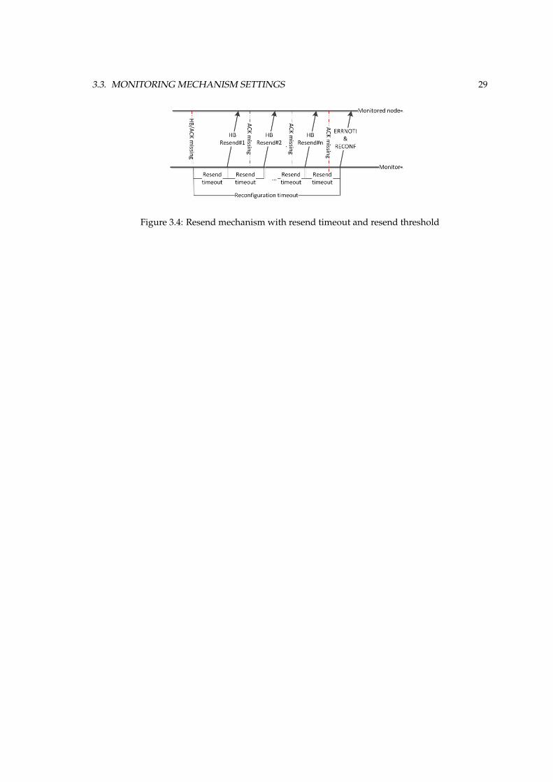
Resend mechanism affects the fault response time and detection accuracy. It contains two values,resend timeout and resend threshold, as seen in figure 3.4. Resend timeout is the duration from whena missing HB is expected to when a HB request is resent. Resend threshold is the maximum countsof resending HBs (n). If the threshold is reached and there is no response from the monitorednode, the reconfiguration will be initiated. Resend threshold is only implemented in the resendmechanism of PULL and PUSH-PULL model, when the mechanism switches to PULL becausePULL HB is a reliable message. As mentioned in subsection 2.1.2, if there is no ACK for the reliablemessage from the receiver, the message or in this case, a PULL HB, will be resent.
In PUSH mechanism, HB is an unreliable message and is initiated from the monitored node, thusthe monitor cannot resend HB request. However, resend timeout can be used in PUSH mechanismby setting resend threshold as 0, consequently, the resend timeout will be used as a reconfigurationtimeout. Reconfiguration timeout is the duration from the start of the first resend timeout until theend of the last one. In other words, it is the duration from the detection of a missing monitoringmessage to the reconfiguration.
3.3. MONITORING MECHANISM SETTINGS 29
Figure 3.4: Resend mechanism with resend timeout and resend threshold

Chapter 4
Simulation Specification and Implementa-tion
This chapter shows the simulation specifications of monitoring models, which are designed in theprevious chapter. It begins in section 4.1 with the introduction to OMNeT++, which is the simu-lation tool used for implementing and testing the models. Afterwards, the simulation objectivesand the performance indicators are explained in section 4.2 and 4.3. The details of how OBC-NGsystem is simulated are shown in section 4.4. Section 4.5 presents the implementation of monitor-ing mechanisms on OBC-NG system. The mechanism and environment settings simulation areexplained in section 4.6 and 4.7. Section 4.8 describes how to the simulations are executed. Finally,the five test suites, which combine each monitoring mechanism, its settings and environmentsettings, are explained in the last section.
4.1 Simulation Tool: OMNeT++
OMNeT++ is an object-oriented discrete event network simulation framework. It is not a simulatorbut it provides infrastructure, libraries and frameworks for the simulation. Its modular architecturedivides the network models into modular and reusable components. Each active component in thesimulation model is called a simple module, which is a basic unit of other compound modules andmodels. The modules are connected via a channel [29]. In addition, it also uses message-triggeredand event-triggered mechanisms as OBC-NG middleware as mention in subsection 2.1.2.
The main functions of the class cSimpleModule are initialize and handleMessage. The first oneis invoked by the simulation kernel once at the beginning and the second one at each messagearrival. Messages, packets and events are all represented by cMessage objects. Most models needto schedule future events in order to implement timers, timeouts, and delays. It can be done insimple module by sending a self-message to itself. After the self-message is sent or scheduled, it will
31
32 CHAPTER 4. SIMULATION SPECIFICATION AND IMPLEMENTATION
be held by the simulation kernel until the schedule time is reached then the message is deliveredto the modules via handleMessage [29]. Since the simulation kernel is event based, the event can bescheduled at different points in real time to the same simulation time. When the simulation time isreached, it is seen as the events are executed in parallel.
4.1.1 OMNeT++ Components Specifications
The behaviors and designs of the components are specified in different types of files [30].
• .ned file: NED or Network Description is a high-level language that describes the structure ofthe modules at every level, from simple module to a model. It also describes the parameters,gates, and network topology of the model.
• .cc file: The file contains the behaviors of each module, which are specified in C++ language.
• .msg file: The communication between module is via messages. Message Definitions file isfor defining various types of message or packet and specifying data fields. OMNeT++ willtranslate message definitions into C++ classes.
• .ini file or a configuration file contains the configurations of the model and different parame-ters of each simulation run.
4.1.2 OMNeT++ User Interfaces
The simulations can be run using Tkenv or Cmdenv user interfaces. Tkenv is a GUI toolkitand graphical simulation environment, which links into simulation executables for graphicalinteractive simulation execution. It is very useful for model development and verification. Cmdenvis a command-line user interface for batch execution. It can be used to execute many runs by onecommand [29].
4.1.3 Output Formats and Types
The output of simulation can be recorded as vector or scalar. Vector output is recorded duringthe simulation into output vector file (.vec). The scalar values are collected during the simulationin a variable and recorded at the end of the simulation in output scalar file (.sca). Moreover, ifthe simulation is run with record event log option, the sequence chart is produced and storedin event log file (.elog). It contains the graphical view of modules, events and messages sequenceand transmission duration. The first three types of output files can be exported as Scalable VectorGraphics file (.svg) [30].
4.2. SIMULATION OBJECTIVES 33
4.2 Simulation Objectives
Two main objectives of the simulation are to evaluate the monitoring efficiency and to measure theoverhead of different monitoring mechanisms and their settings. They are tested under differentenvironment settings, i.e. high network load and node failures. Fault injection is simulated inorder to see how fast the monitoring system reacts when different type of nodes fail at differentfault injection time. The outcomes of simulation are used to evaluate different monitoring designoptions for OBC-NG system.
4.3 Performance Indicators
Performance indicators are used to measure the efficiency of the monitoring models. They arechosen according to the OBC-NG monitoring requirements from section 3.1 to prevent the funda-mental problems of distributed system monitoring, which are previously presented in subsection2.3.2.
4.3.1 Monitoring Overhead
An efficient monitoring system should create as low overhead as possible. The bandwidth con-sumption is measured to specify the communication overhead and the total number of monitoringmessages sent from each node to measure the workload on different roles. Both HB and ACKare measured over the simulation time. CPU overhead is not simulated because in the currentimplementation, every node in the network is COTS component and therefore it is assumed thatthe computing power is sufficient.
4.3.2 Fault Response Time
Fault response time in this work is the duration between fault injection time and when the re-maining healthy nodes receive reconfiguration messages. It is right before the reconfigurationmechanism starts and the nodes handle the reconfiguration messages. At the end of each simula-tion, the difference between the simulation times of those two events is recorded.
4.3.3 Monitoring System Stability
Monitoring system stability is the ability to avoid incorrect judgment and running into a wrongconfiguration, when there is high network load in the system. The system starts up in the initialconfiguration with configuration ID = 0. In the test without node failure, the reconfiguration
34 CHAPTER 4. SIMULATION SPECIFICATION AND IMPLEMENTATION
should not be triggered. If the monitor searches the decision graph for the next configuration andtries to initiate reconfiguration by sending reconfiguration message with configuration ID 6= 0, thetimestamp is recorded and endSimulation function is called.
4.4 OBC-NG System Simulation
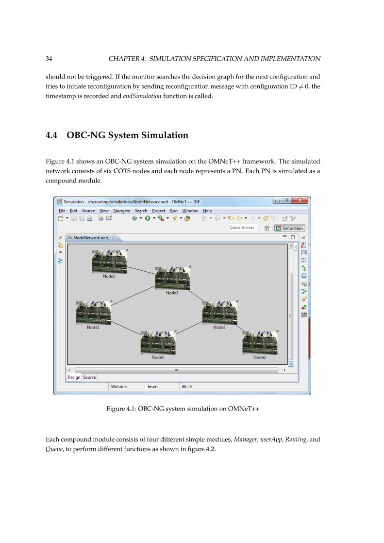
Figure 4.1 shows an OBC-NG system simulation on the OMNeT++ framework. The simulatednetwork consists of six COTS nodes and each node represents a PN. Each PN is simulated as acompound module.
Figure 4.1: OBC-NG system simulation on OMNeT++
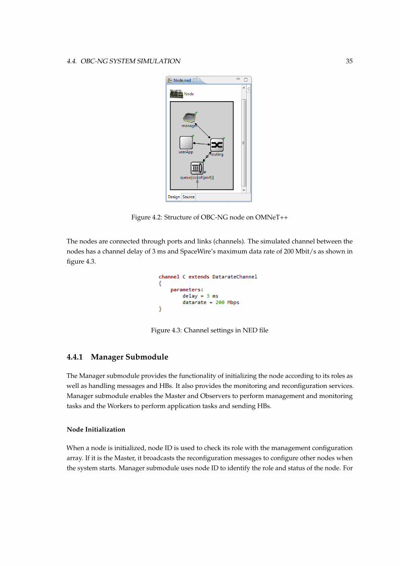
Each compound module consists of four different simple modules, Manager, userApp, Routing, andQueue, to perform different functions as shown in figure 4.2.
4.4. OBC-NG SYSTEM SIMULATION 35
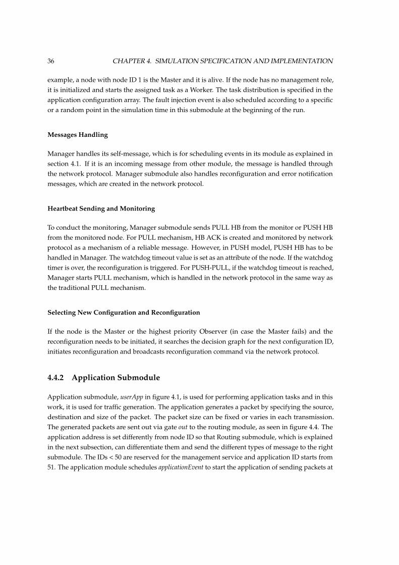
Figure 4.2: Structure of OBC-NG node on OMNeT++
The nodes are connected through ports and links (channels). The simulated channel between thenodes has a channel delay of 3 ms and SpaceWire’s maximum data rate of 200 Mbit/s as shown infigure 4.3.
Figure 4.3: Channel settings in NED file
4.4.1 Manager Submodule
The Manager submodule provides the functionality of initializing the node according to its roles aswell as handling messages and HBs. It also provides the monitoring and reconfiguration services.Manager submodule enables the Master and Observers to perform management and monitoringtasks and the Workers to perform application tasks and sending HBs.
Node Initialization
When a node is initialized, node ID is used to check its role with the management configurationarray. If it is the Master, it broadcasts the reconfiguration messages to configure other nodes whenthe system starts. Manager submodule uses node ID to identify the role and status of the node. For
36 CHAPTER 4. SIMULATION SPECIFICATION AND IMPLEMENTATION
example, a node with node ID 1 is the Master and it is alive. If the node has no management role,it is initialized and starts the assigned task as a Worker. The task distribution is specified in theapplication configuration array. The fault injection event is also scheduled according to a specificor a random point in the simulation time in this submodule at the beginning of the run.
Messages Handling
Manager handles its self-message, which is for scheduling events in its module as explained insection 4.1. If it is an incoming message from other module, the message is handled throughthe network protocol. Manager submodule also handles reconfiguration and error notificationmessages, which are created in the network protocol.
Heartbeat Sending and Monitoring
To conduct the monitoring, Manager submodule sends PULL HB from the monitor or PUSH HBfrom the monitored node. For PULL mechanism, HB ACK is created and monitored by networkprotocol as a mechanism of a reliable message. However, in PUSH model, PUSH HB has to behandled in Manager. The watchdog timeout value is set as an attribute of the node. If the watchdogtimer is over, the reconfiguration is triggered. For PUSH-PULL, if the watchdog timeout is reached,Manager starts PULL mechanism, which is handled in the network protocol in the same way asthe traditional PULL mechanism.
Selecting New Configuration and Reconfiguration
If the node is the Master or the highest priority Observer (in case the Master fails) and thereconfiguration needs to be initiated, it searches the decision graph for the next configuration ID,initiates reconfiguration and broadcasts reconfiguration command via the network protocol.
4.4.2 Application Submodule
Application submodule, userApp in figure 4.1, is used for performing application tasks and in thiswork, it is used for traffic generation. The application generates a packet by specifying the source,destination and size of the packet. The packet size can be fixed or varies in each transmission.The generated packets are sent out via gate out to the routing module, as seen in figure 4.4. Theapplication address is set differently from node ID so that Routing submodule, which is explainedin the next subsection, can differentiate them and send the different types of message to the rightsubmodule. The IDs < 50 are reserved for the management service and application ID starts from51. The application module schedules applicationEvent to start the application of sending packets at
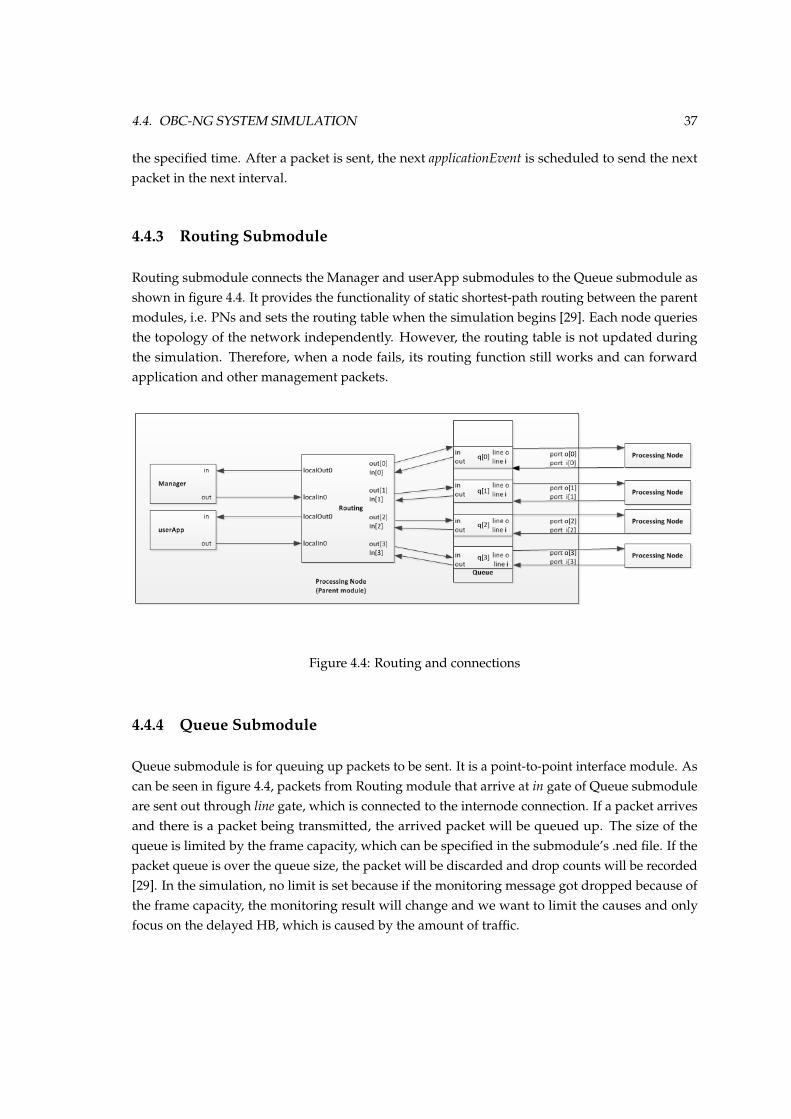
4.4. OBC-NG SYSTEM SIMULATION 37
the specified time. After a packet is sent, the next applicationEvent is scheduled to send the nextpacket in the next interval.
4.4.3 Routing Submodule
Routing submodule connects the Manager and userApp submodules to the Queue submodule asshown in figure 4.4. It provides the functionality of static shortest-path routing between the parentmodules, i.e. PNs and sets the routing table when the simulation begins [29]. Each node queriesthe topology of the network independently. However, the routing table is not updated duringthe simulation. Therefore, when a node fails, its routing function still works and can forwardapplication and other management packets.
Figure 4.4: Routing and connections
4.4.4 Queue Submodule
Queue submodule is for queuing up packets to be sent. It is a point-to-point interface module. Ascan be seen in figure 4.4, packets from Routing module that arrive at in gate of Queue submoduleare sent out through line gate, which is connected to the internode connection. If a packet arrivesand there is a packet being transmitted, the arrived packet will be queued up. The size of thequeue is limited by the frame capacity, which can be specified in the submodule’s .ned file. If thepacket queue is over the queue size, the packet will be discarded and drop counts will be recorded[29]. In the simulation, no limit is set because if the monitoring message got dropped because ofthe frame capacity, the monitoring result will change and we want to limit the causes and onlyfocus on the delayed HB, which is caused by the amount of traffic.
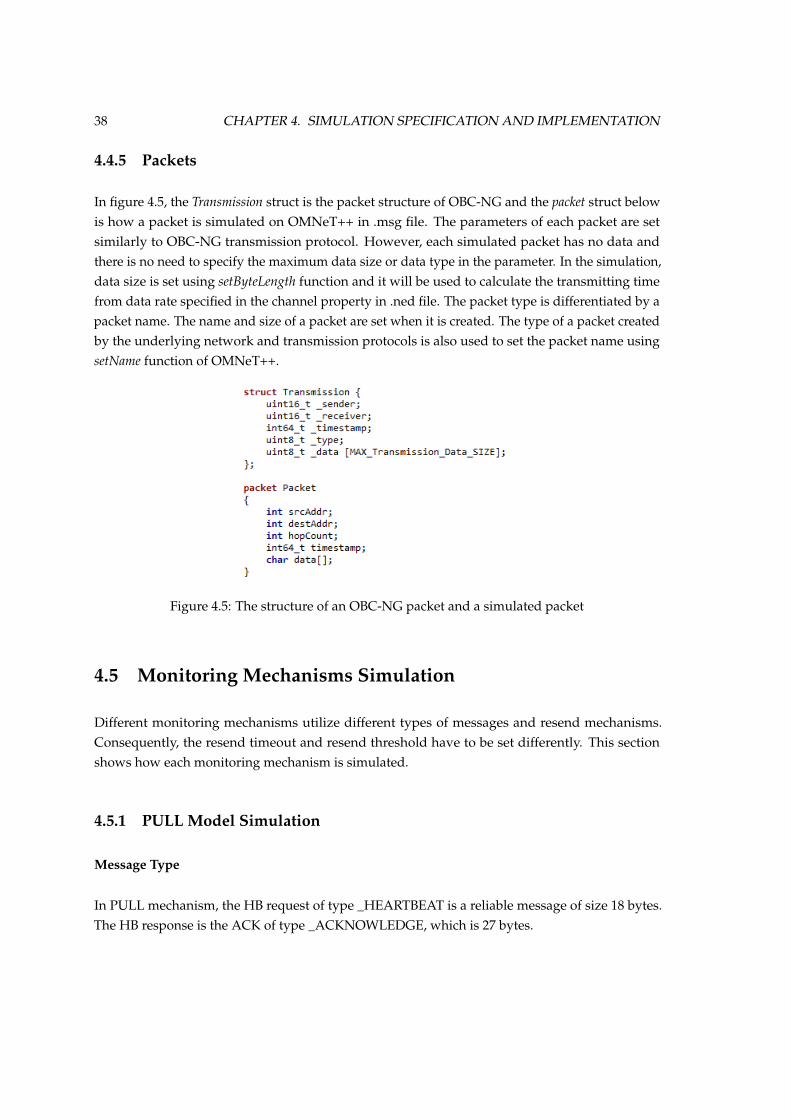
38 CHAPTER 4. SIMULATION SPECIFICATION AND IMPLEMENTATION
4.4.5 Packets
In figure 4.5, the Transmission struct is the packet structure of OBC-NG and the packet struct belowis how a packet is simulated on OMNeT++ in .msg file. The parameters of each packet are setsimilarly to OBC-NG transmission protocol. However, each simulated packet has no data andthere is no need to specify the maximum data size or data type in the parameter. In the simulation,data size is set using setByteLength function and it will be used to calculate the transmitting timefrom data rate specified in the channel property in .ned file. The packet type is differentiated by apacket name. The name and size of a packet are set when it is created. The type of a packet createdby the underlying network and transmission protocols is also used to set the packet name usingsetName function of OMNeT++.
Figure 4.5: The structure of an OBC-NG packet and a simulated packet
4.5 Monitoring Mechanisms Simulation
Different monitoring mechanisms utilize different types of messages and resend mechanisms.Consequently, the resend timeout and resend threshold have to be set differently. This sectionshows how each monitoring mechanism is simulated.
4.5.1 PULL Model Simulation
Message Type
In PULL mechanism, the HB request of type _HEARTBEAT is a reliable message of size 18 bytes.The HB response is the ACK of type _ACKNOWLEDGE, which is 27 bytes.
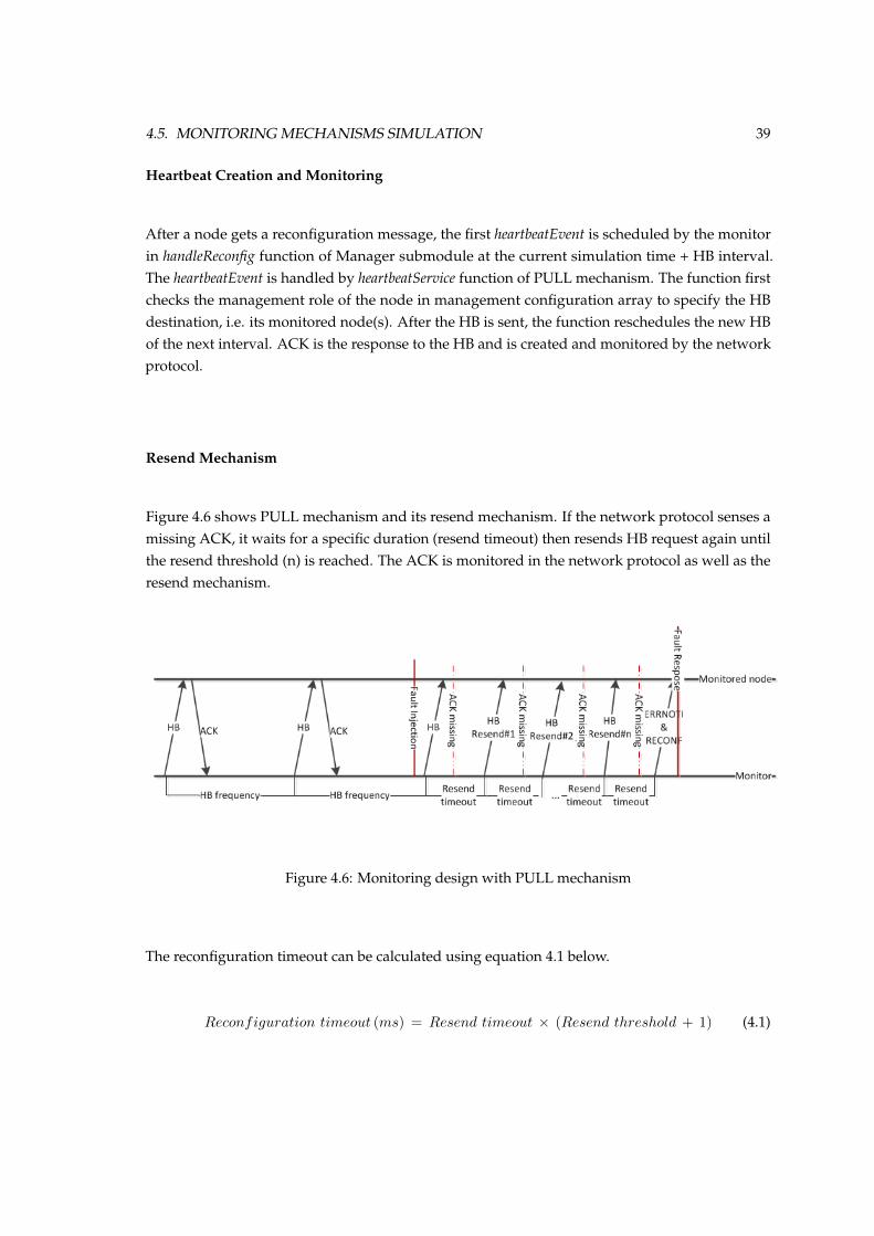
4.5. MONITORING MECHANISMS SIMULATION 39
Heartbeat Creation and Monitoring
After a node gets a reconfiguration message, the first heartbeatEvent is scheduled by the monitorin handleReconfig function of Manager submodule at the current simulation time + HB interval.The heartbeatEvent is handled by heartbeatService function of PULL mechanism. The function firstchecks the management role of the node in management configuration array to specify the HBdestination, i.e. its monitored node(s). After the HB is sent, the function reschedules the new HBof the next interval. ACK is the response to the HB and is created and monitored by the networkprotocol.
Resend Mechanism
Figure 4.6 shows PULL mechanism and its resend mechanism. If the network protocol senses amissing ACK, it waits for a specific duration (resend timeout) then resends HB request again untilthe resend threshold (n) is reached. The ACK is monitored in the network protocol as well as theresend mechanism.
Figure 4.6: Monitoring design with PULL mechanism
The reconfiguration timeout can be calculated using equation 4.1 below.
Reconfiguration timeout (ms) = Resend timeout ⇥ (Resend threshold + 1) (4.1)
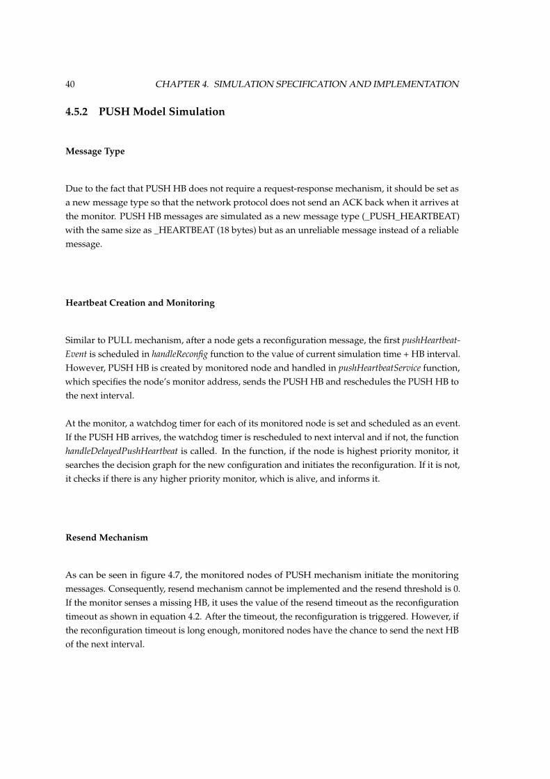
40 CHAPTER 4. SIMULATION SPECIFICATION AND IMPLEMENTATION
4.5.2 PUSH Model Simulation
Message Type
Due to the fact that PUSH HB does not require a request-response mechanism, it should be set asa new message type so that the network protocol does not send an ACK back when it arrives atthe monitor. PUSH HB messages are simulated as a new message type (_PUSH_HEARTBEAT)with the same size as _HEARTBEAT (18 bytes) but as an unreliable message instead of a reliablemessage.
Heartbeat Creation and Monitoring
Similar to PULL mechanism, after a node gets a reconfiguration message, the first pushHeartbeat-Event is scheduled in handleReconfig function to the value of current simulation time + HB interval.However, PUSH HB is created by monitored node and handled in pushHeartbeatService function,which specifies the node’s monitor address, sends the PUSH HB and reschedules the PUSH HB tothe next interval.
At the monitor, a watchdog timer for each of its monitored node is set and scheduled as an event.If the PUSH HB arrives, the watchdog timer is rescheduled to next interval and if not, the functionhandleDelayedPushHeartbeat is called. In the function, if the node is highest priority monitor, itsearches the decision graph for the new configuration and initiates the reconfiguration. If it is not,it checks if there is any higher priority monitor, which is alive, and informs it.
Resend Mechanism
As can be seen in figure 4.7, the monitored nodes of PUSH mechanism initiate the monitoringmessages. Consequently, resend mechanism cannot be implemented and the resend threshold is 0.If the monitor senses a missing HB, it uses the value of the resend timeout as the reconfigurationtimeout as shown in equation 4.2. After the timeout, the reconfiguration is triggered. However, ifthe reconfiguration timeout is long enough, monitored nodes have the chance to send the next HBof the next interval.
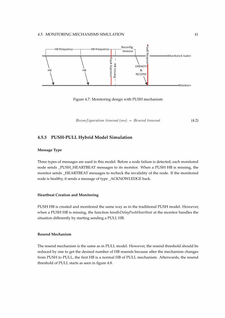
4.5. MONITORING MECHANISMS SIMULATION 41
Figure 4.7: Monitoring design with PUSH mechanism
Reconfiguration timeout (ms) = Resend timeout (4.2)
4.5.3 PUSH-PULL Hybrid Model Simulation
Message Type
Three types of messages are used in this model. Before a node failure is detected, each monitorednode sends _PUSH_HEARTBEAT messages to its monitor. When a PUSH HB is missing, themonitor sends _HEARTBEAT messages to recheck the invalidity of the node. If the monitorednode is healthy, it sends a message of type _ACKNOWLEDGE back.
Heartbeat Creation and Monitoring
PUSH HB is created and monitored the same way as in the traditional PUSH model. However,when a PUSH HB is missing, the function handleDelayPushHeartbeat at the monitor handles thesituation differently by starting sending a PULL HB.
Resend Mechanism
The resend mechanism is the same as in PULL model. However, the resend threshold should bereduced by one to get the desired number of HB resends because after the mechanism changesfrom PUSH to PULL, the first HB is a normal HB of PULL mechanism. Afterwards, the resendthreshold of PULL starts as seen in figure 4.8.
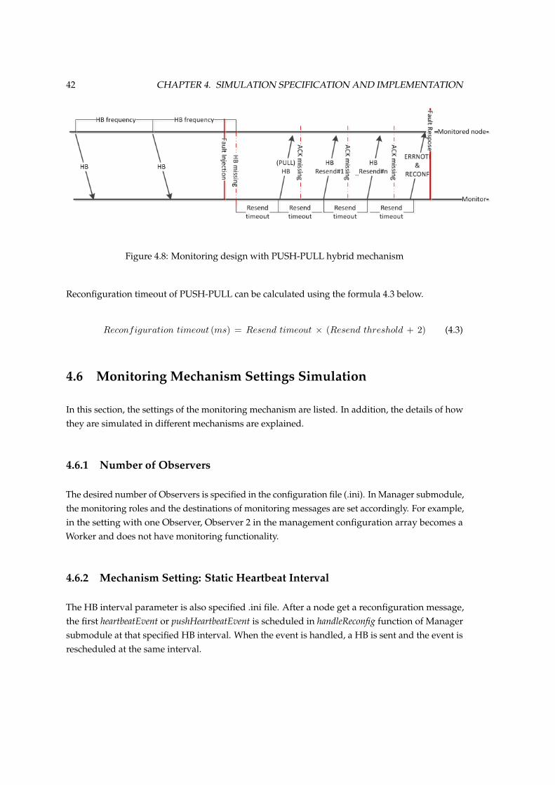
42 CHAPTER 4. SIMULATION SPECIFICATION AND IMPLEMENTATION
Figure 4.8: Monitoring design with PUSH-PULL hybrid mechanism
Reconfiguration timeout of PUSH-PULL can be calculated using the formula 4.3 below.
Reconfiguration timeout (ms) = Resend timeout ⇥ (Resend threshold + 2) (4.3)
4.6 Monitoring Mechanism Settings Simulation
In this section, the settings of the monitoring mechanism are listed. In addition, the details of howthey are simulated in different mechanisms are explained.
4.6.1 Number of Observers
The desired number of Observers is specified in the configuration file (.ini). In Manager submodule,the monitoring roles and the destinations of monitoring messages are set accordingly. For example,in the setting with one Observer, Observer 2 in the management configuration array becomes aWorker and does not have monitoring functionality.
4.6.2 Mechanism Setting: Static Heartbeat Interval
The HB interval parameter is also specified .ini file. After a node get a reconfiguration message,the first heartbeatEvent or pushHeartbeatEvent is scheduled in handleReconfig function of Managersubmodule at that specified HB interval. When the event is handled, a HB is sent and the event isrescheduled at the same interval.
4.7. ENVIRONMENT SETTINGS SIMULATION 43
4.6.3 Mechanism Setting: Dynamic Heartbeat Interval
There are two options of simulating dynamic HB. The first approach is to measure network trafficand adjust HB interval accordingly. In PULL mechanism, the monitor changes the interval ofthe HB request, and in PUSH, the monitor sends a message to the monitored node to change theinterval of the next HB to prevent the synchronization issue. The monitor node itself changes theduration of the watchdog timer to prepare itself for the new interval. The disadvantage of thisapproach is, the change occurs at the next HB interval and it might be too late to adapt to thenetwork traffic.
Another approach is to adjust the watchdog timer according to the previous HB arrival. The newwatchdog timer is set when the HB arrives. The simulation times of the previous and the currentHB arrivals are recorded. The difference between these two values is added with a slack time tocalculate a new watchdog timer. The slack time is calculated using the equation 4.4 below. Theslack factor makes the next interval slightly larger than the actual difference of the HB arrivals toprepare for higher network traffic. In this case, the monitor can sense the traffic and adjust thewatchdog timer accordingly.
Slack time (ms) = (simulation time of currentHB arrival� previousHB arrival)⇥ slack factor
(4.4)
4.7 Environment Settings Simulation
4.7.1 Fault Injection: Node Failure
Node failure is simulated by scheduling a faultInjectionEvent, which is handled by the chosennode at the scheduled time. At the chosen node, its isAlive status is updated to false and it willstop sending HBs. On Tkenv GUI, the node is labeled as dead. The purpose of fault injection ismeasuring fault response time of each mechanism.
In the design, a random failure is injected in each simulation randomly because random failureswith constant failure rate are used for calculating MTTR. The duration between fault injection andfault response time of each mechanism is recorded. However, a fault is supposed to be detectedwithin the simulation time (5000 ms) so that the fault response time can be recorded. Therefore,the failures are random in the range of 0 - 4000 ms to make sure that they will be detected in everyHB interval setting.
The random function rand is used with the seed of wall-clock time, which is specified in srandfunction as srand(time(NULL)). It is used to generate random number for fault injection time and
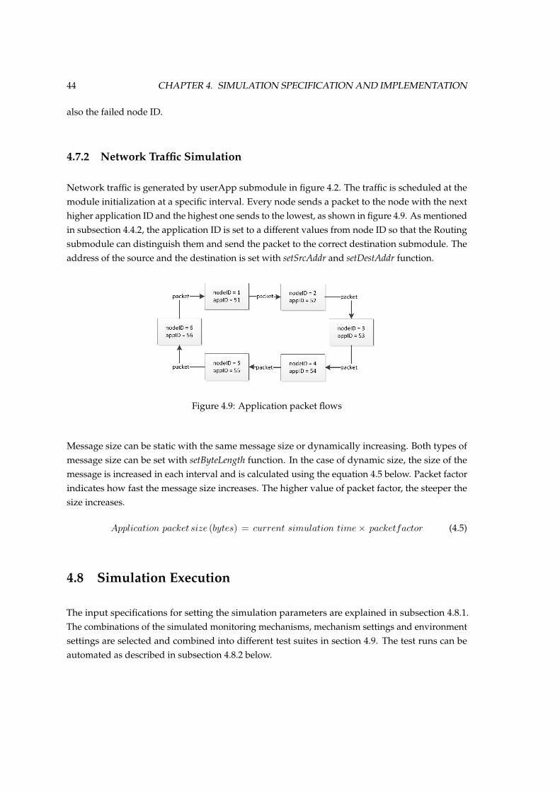
44 CHAPTER 4. SIMULATION SPECIFICATION AND IMPLEMENTATION
also the failed node ID.
4.7.2 Network Traffic Simulation
Network traffic is generated by userApp submodule in figure 4.2. The traffic is scheduled at themodule initialization at a specific interval. Every node sends a packet to the node with the nexthigher application ID and the highest one sends to the lowest, as shown in figure 4.9. As mentionedin subsection 4.4.2, the application ID is set to a different values from node ID so that the Routingsubmodule can distinguish them and send the packet to the correct destination submodule. Theaddress of the source and the destination is set with setSrcAddr and setDestAddr function.
Figure 4.9: Application packet flows
Message size can be static with the same message size or dynamically increasing. Both types ofmessage size can be set with setByteLength function. In the case of dynamic size, the size of themessage is increased in each interval and is calculated using the equation 4.5 below. Packet factorindicates how fast the message size increases. The higher value of packet factor, the steeper thesize increases.
Application packet size (bytes) = current simulation time⇥ packetfactor (4.5)
4.8 Simulation Execution
The input specifications for setting the simulation parameters are explained in subsection 4.8.1.The combinations of the simulated monitoring mechanisms, mechanism settings and environmentsettings are selected and combined into different test suites in section 4.9. The test runs can beautomated as described in subsection 4.8.2 below.
4.9. TEST SUITES 45
4.8.1 Input Specifications
Most test settings are specified as parameter values or seeds in the configuration file (.ini). However,the resend threshold and resend timeout are specified as macros since the resend mechanism isprovided by the underlying network protocol, not an OMNeT++ module.
4.8.2 Automated Tests
Instead of executing each test case manually, automated tests can be performed to execute everytest case in each test suite. The parameter values of each test case settings can be specifiedin the configuration file. Then change the run configurations in the Integrated DevelopmentEnvironment (IDE) to command line and change run number to * to run all the test cases withevery parameter combinations.
4.9 Test Suites
The monitoring system testing is divided into five test suites according to the test objectives. Thefirst test suite compares the monitoring overhead and the fault response time of the PULL andPUSH mechanisms without the resend mechanism. The second test suite aims to compare thesettings with different number of Observers. The third and fourth test suites test the monitoringmodels under different environment settings, i.e. fault injection and network traffic. Finally, thefifth test suite verifies the dynamic HB mechanism.
Test suite 1: Monitoring Mechanisms and Observer Roles
General Purpose
This test aims to compare PULL and PUSH mechanisms without resend mechanism by usingthe same mechanism settings. Different monitoring roles of the Observers are also tested. Theevaluation focuses on the monitoring overhead, workload of each role, and fault response time.

46 CHAPTER 4. SIMULATION SPECIFICATION AND IMPLEMENTATION
General Configurations
Table 4.1: Test suite 1 General configurations
Mechanism PULL, PUSH
Number of Observers (nodes) 2
Heartbeat interval (ms) Static: every 200
Reconfiguration timeout (ms) 30
Resend threshold (times) 0
Node failures See the test case settings below
Application traffic None
Simulation time limit (ms) 5000
Test case settings
Table 4.2: Test suite 1 Test case settings
TestID Node failure Test details
1.1.10 node failure
Observer role setting 1: O2 Observes M and O11.1.2 Observer role setting 2: O2 Observes only O11.2 1 node failure Each role fails at 1000 ms
Test Suite 2: Number of Observers
General Purpose
In the previous test, the default number of Observers (two nodes) is tested with different Observerrole settings. The chosen setting is used in this test and the following tests. The goal of this test isto compare fault response time of the settings with different number of Observers when the Masterfails.
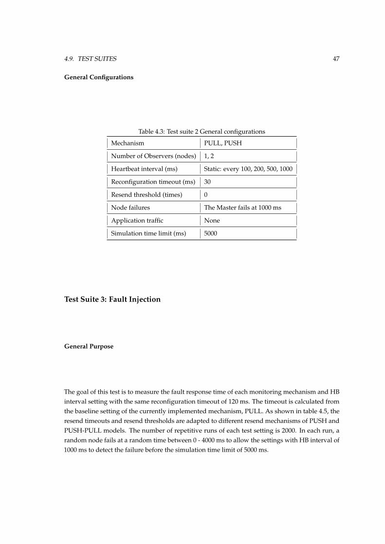
4.9. TEST SUITES 47
General Configurations
Table 4.3: Test suite 2 General configurations
Mechanism PULL, PUSH
Number of Observers (nodes) 1, 2
Heartbeat interval (ms) Static: every 100, 200, 500, 1000
Reconfiguration timeout (ms) 30
Resend threshold (times) 0
Node failures The Master fails at 1000 ms
Application traffic None
Simulation time limit (ms) 5000
Test Suite 3: Fault Injection
General Purpose
The goal of this test is to measure the fault response time of each monitoring mechanism and HBinterval setting with the same reconfiguration timeout of 120 ms. The timeout is calculated fromthe baseline setting of the currently implemented mechanism, PULL. As shown in table 4.5, theresend timeouts and resend thresholds are adapted to different resend mechanisms of PUSH andPUSH-PULL models. The number of repetitive runs of each test setting is 2000. In each run, arandom node fails at a random time between 0 - 4000 ms to allow the settings with HB interval of1000 ms to detect the failure before the simulation time limit of 5000 ms.
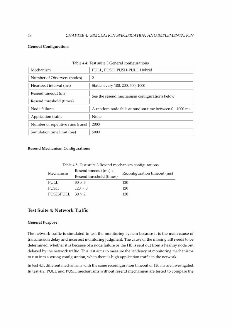
48 CHAPTER 4. SIMULATION SPECIFICATION AND IMPLEMENTATION
General Configurations
Table 4.4: Test suite 3 General configurations
Mechanism PULL, PUSH, PUSH-PULL Hybrid
Number of Observers (nodes) 2
Heartbeat interval (ms) Static: every 100, 200, 500, 1000
Resend timeout (ms)See the resend mechanism configurations below
Resend threshold (times)
Node failures A random node fails at random time between 0 - 4000 ms
Application traffic None
Number of repetitive runs (runs) 2000
Simulation time limit (ms) 5000
Resend Mechanism Configurations
Table 4.5: Test suite 3 Resend mechanism configurations
MechanismResend timeout (ms) xResend threshold (times)
Reconfiguration timeout (ms)
PULL 30 ⇥ 3 120PUSH 120 ⇥ 0 120PUSH-PULL 30 ⇥ 2 120
Test Suite 4: Network Traffic
General Purpose
The network traffic is simulated to test the monitoring system because it is the main cause oftransmission delay and incorrect monitoring judgment. The cause of the missing HB needs to bedetermined, whether it is because of a node failure or the HB is sent out from a healthy node butdelayed by the network traffic. This test aims to measure the tendency of monitoring mechanismsto run into a wrong configuration, when there is high application traffic in the network.
In test 4.1, different mechanisms with the same reconfiguration timeout of 120 ms are investigated.In test 4.2, PULL and PUSH mechanisms without resend mechanism are tested to compare the
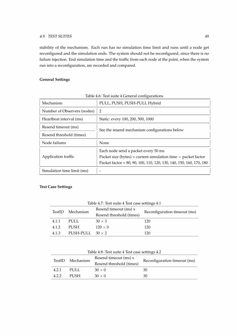
4.9. TEST SUITES 49
stability of the mechanism. Each run has no simulation time limit and runs until a node getreconfigured and the simulation ends. The system should not be reconfigured, since there is nofailure injection. End simulation time and the traffic from each node at the point, when the systemrun into a reconfiguration, are recorded and compared.
General Settings
Table 4.6: Test suite 4 General configurations
Mechanism PULL, PUSH, PUSH-PULL Hybrid
Number of Observers (nodes) 2
Heartbeat interval (ms) Static: every 100, 200, 500, 1000
Resend timeout (ms)See the resend mechanism configurations below
Resend threshold (times)
Node failures None
Application trafficEach node send a packet every 50 msPacket size (bytes) = current simulation time ⇥ packet factorPacket factor = 80, 90, 100, 110, 120, 130, 140, 150, 160, 170, 180
Simulation time limit (ms) -
Test Case Settings
Table 4.7: Test suite 4 Test case settings 4.1
TestID MechanismResend timeout (ms) xResend threshold (times)
Reconfiguration timeout (ms)
4.1.1 PULL 30 ⇥ 3 1204.1.2 PUSH 120 ⇥ 0 1204.1.3 PUSH-PULL 30 ⇥ 2 120
Table 4.8: Test suite 4 Test case settings 4.2
TestID MechanismResend timeout (ms) xResend threshold (times)
Reconfiguration timeout (ms)
4.2.1 PULL 30 ⇥ 0 304.2.2 PUSH 30 ⇥ 0 30
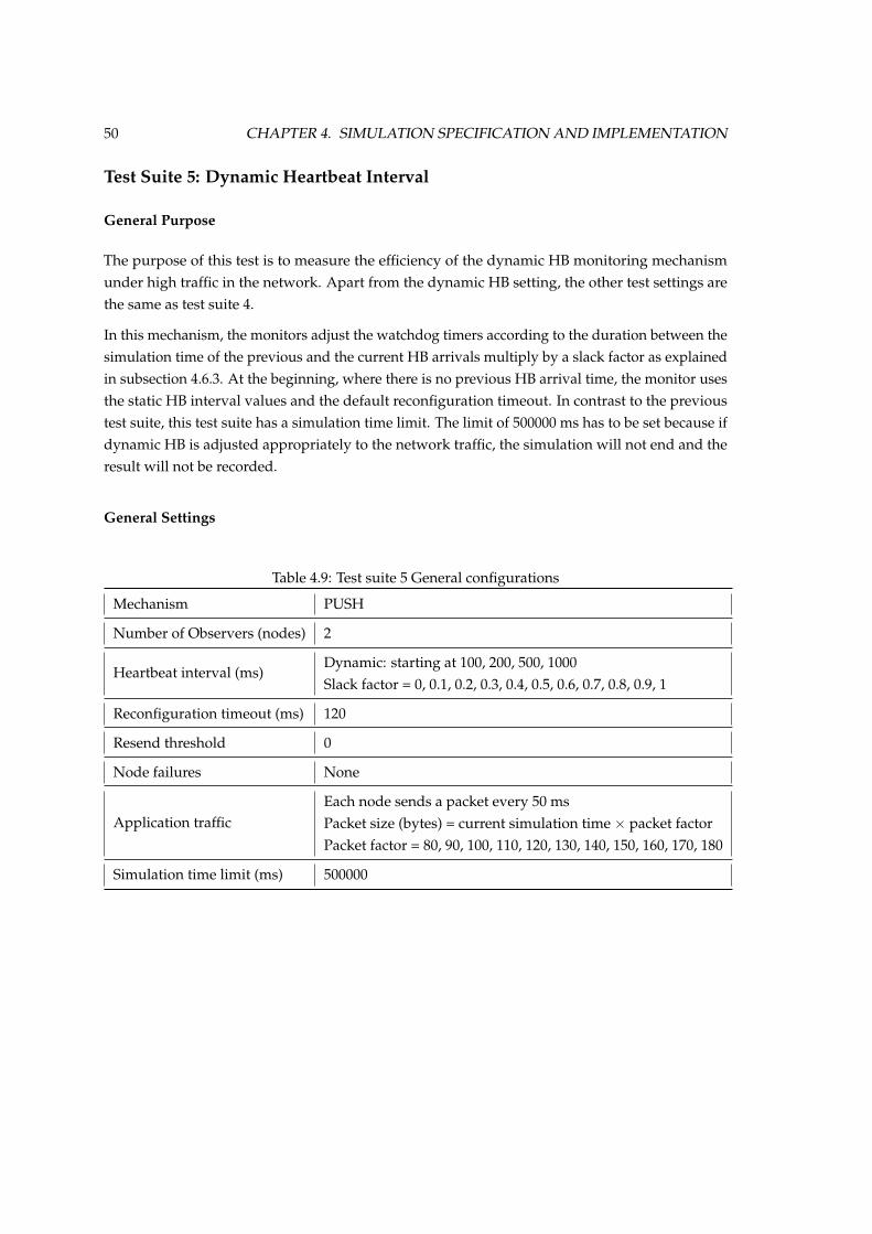
50 CHAPTER 4. SIMULATION SPECIFICATION AND IMPLEMENTATION
Test Suite 5: Dynamic Heartbeat Interval
General Purpose
The purpose of this test is to measure the efficiency of the dynamic HB monitoring mechanismunder high traffic in the network. Apart from the dynamic HB setting, the other test settings arethe same as test suite 4.
In this mechanism, the monitors adjust the watchdog timers according to the duration between thesimulation time of the previous and the current HB arrivals multiply by a slack factor as explainedin subsection 4.6.3. At the beginning, where there is no previous HB arrival time, the monitor usesthe static HB interval values and the default reconfiguration timeout. In contrast to the previoustest suite, this test suite has a simulation time limit. The limit of 500000 ms has to be set because ifdynamic HB is adjusted appropriately to the network traffic, the simulation will not end and theresult will not be recorded.
General Settings
Table 4.9: Test suite 5 General configurations
Mechanism PUSH
Number of Observers (nodes) 2
Heartbeat interval (ms)Dynamic: starting at 100, 200, 500, 1000Slack factor = 0, 0.1, 0.2, 0.3, 0.4, 0.5, 0.6, 0.7, 0.8, 0.9, 1
Reconfiguration timeout (ms) 120
Resend threshold 0
Node failures None
Application trafficEach node sends a packet every 50 msPacket size (bytes) = current simulation time ⇥ packet factorPacket factor = 80, 90, 100, 110, 120, 130, 140, 150, 160, 170, 180
Simulation time limit (ms) 500000
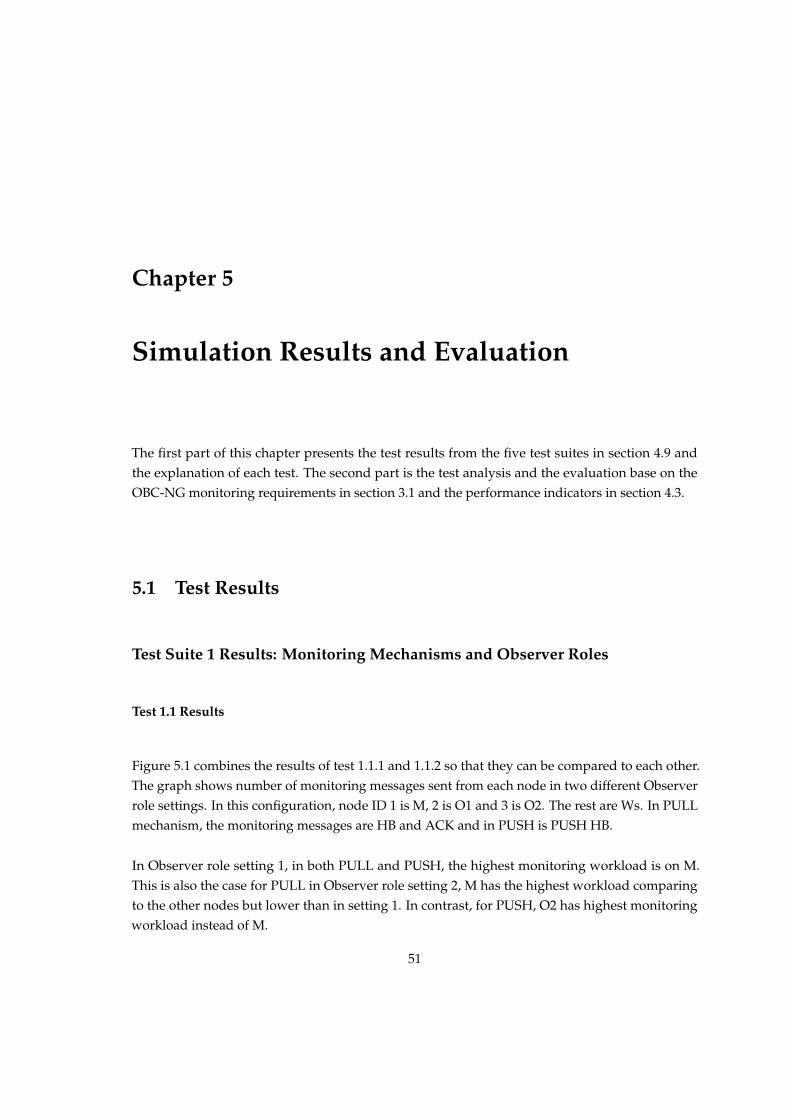
Chapter 5
Simulation Results and Evaluation
The first part of this chapter presents the test results from the five test suites in section 4.9 andthe explanation of each test. The second part is the test analysis and the evaluation base on theOBC-NG monitoring requirements in section 3.1 and the performance indicators in section 4.3.
5.1 Test Results
Test Suite 1 Results: Monitoring Mechanisms and Observer Roles
Test 1.1 Results
Figure 5.1 combines the results of test 1.1.1 and 1.1.2 so that they can be compared to each other.The graph shows number of monitoring messages sent from each node in two different Observerrole settings. In this configuration, node ID 1 is M, 2 is O1 and 3 is O2. The rest are Ws. In PULLmechanism, the monitoring messages are HB and ACK and in PUSH is PUSH HB.
In Observer role setting 1, in both PULL and PUSH, the highest monitoring workload is on M.This is also the case for PULL in Observer role setting 2, M has the highest workload comparingto the other nodes but lower than in setting 1. In contrast, for PUSH, O2 has highest monitoringworkload instead of M.
51
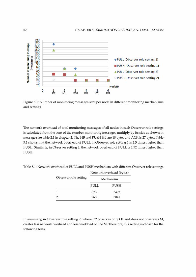
52 CHAPTER 5. SIMULATION RESULTS AND EVALUATION
Figure 5.1: Number of monitoring messages sent per node in different monitoring mechanismsand settings
The network overhead of total monitoring messages of all nodes in each Observer role settingsis calculated from the sum of the number monitoring messages multiply by its size as shown inmessage size table 2.1 in chapter 2. The HB and PUSH HB are 18 bytes and ACK is 27 bytes. Table5.1 shows that the network overhead of PULL in Observer role setting 1 is 2.5 times higher thanPUSH. Similarly, in Observer setting 2, the network overhead of PULL is 2.52 times higher thanPUSH.
Table 5.1: Network overhead of PULL and PUSH mechanism with different Observer role settings
Observer role settingNetwork overhead (bytes)
Mechanism
PULL PUSH
1 8730 34922 7650 3041
In summary, in Observer role setting 2, where O2 observes only O1 and does not observers M,creates less network overhead and less workload on the M. Therefore, this setting is chosen for thefollowing tests.
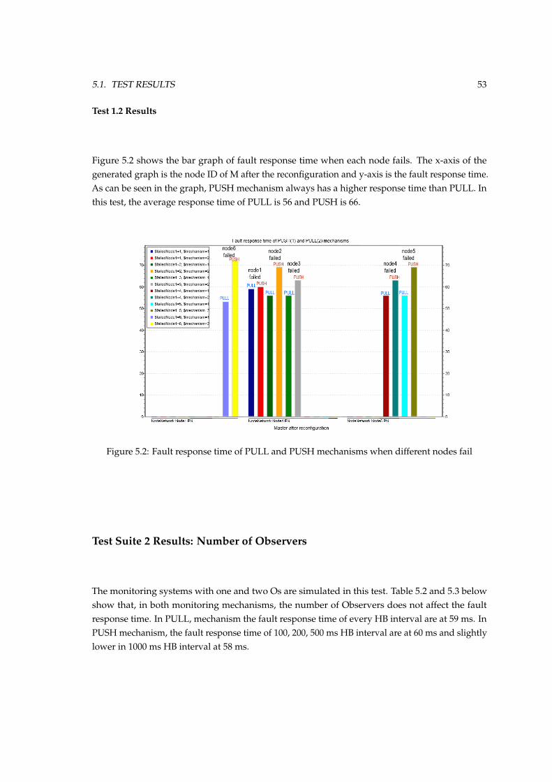
5.1. TEST RESULTS 53
Test 1.2 Results
Figure 5.2 shows the bar graph of fault response time when each node fails. The x-axis of thegenerated graph is the node ID of M after the reconfiguration and y-axis is the fault response time.As can be seen in the graph, PUSH mechanism always has a higher response time than PULL. Inthis test, the average response time of PULL is 56 and PUSH is 66.
Figure 5.2: Fault response time of PULL and PUSH mechanisms when different nodes fail
Test Suite 2 Results: Number of Observers
The monitoring systems with one and two Os are simulated in this test. Table 5.2 and 5.3 belowshow that, in both monitoring mechanisms, the number of Observers does not affect the faultresponse time. In PULL, mechanism the fault response time of every HB interval are at 59 ms. InPUSH mechanism, the fault response time of 100, 200, 500 ms HB interval are at 60 ms and slightlylower in 1000 ms HB interval at 58 ms.
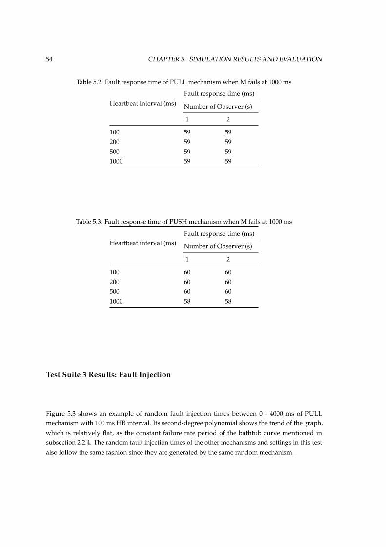
54 CHAPTER 5. SIMULATION RESULTS AND EVALUATION
Table 5.2: Fault response time of PULL mechanism when M fails at 1000 ms
Heartbeat interval (ms)Fault response time (ms)
Number of Observer (s)
1 2
100 59 59200 59 59500 59 591000 59 59
Table 5.3: Fault response time of PUSH mechanism when M fails at 1000 ms
Heartbeat interval (ms)Fault response time (ms)
Number of Observer (s)
1 2
100 60 60200 60 60500 60 601000 58 58
Test Suite 3 Results: Fault Injection
Figure 5.3 shows an example of random fault injection times between 0 - 4000 ms of PULLmechanism with 100 ms HB interval. Its second-degree polynomial shows the trend of the graph,which is relatively flat, as the constant failure rate period of the bathtub curve mentioned insubsection 2.2.4. The random fault injection times of the other mechanisms and settings in this testalso follow the same fashion since they are generated by the same random mechanism.
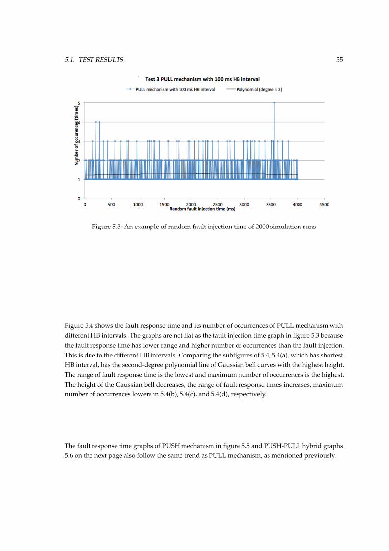
5.1. TEST RESULTS 55
Figure 5.3: An example of random fault injection time of 2000 simulation runs
Figure 5.4 shows the fault response time and its number of occurrences of PULL mechanism withdifferent HB intervals. The graphs are not flat as the fault injection time graph in figure 5.3 becausethe fault response time has lower range and higher number of occurrences than the fault injection.This is due to the different HB intervals. Comparing the subfigures of 5.4, 5.4(a), which has shortestHB interval, has the second-degree polynomial line of Gaussian bell curves with the highest height.The range of fault response time is the lowest and maximum number of occurrences is the highest.The height of the Gaussian bell decreases, the range of fault response times increases, maximumnumber of occurrences lowers in 5.4(b), 5.4(c), and 5.4(d), respectively.
The fault response time graphs of PUSH mechanism in figure 5.5 and PUSH-PULL hybrid graphs5.6 on the next page also follow the same trend as PULL mechanism, as mentioned previously.
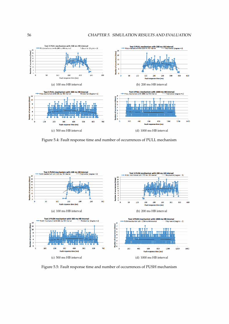
56 CHAPTER 5. SIMULATION RESULTS AND EVALUATION
(a) 100 ms HB interval (b) 200 ms HB interval
(c) 500 ms HB interval (d) 1000 ms HB interval
Figure 5.4: Fault response time and number of occurrences of PULL mechanism
(a) 100 ms HB interval (b) 200 ms HB interval
(c) 500 ms HB interval (d) 1000 ms HB interval
Figure 5.5: Fault response time and number of occurrences of PUSH mechanism
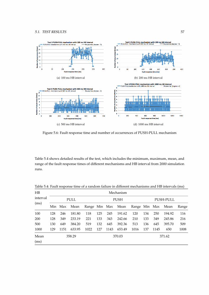
5.1. TEST RESULTS 57
(a) 100 ms HB interval (b) 200 ms HB interval
(c) 500 ms HB interval (d) 1000 ms HB interval
Figure 5.6: Fault response time and number of occurrences of PUSH-PULL mechanism
Table 5.4 shows detailed results of the test, which includes the minimum, maximum, mean, andrange of the fault response times of different mechanisms and HB interval from 2000 simulationruns.
Table 5.4: Fault response time of a random failure in different mechanisms and HB intervals (ms)
HBinterval(ms)
Mechanism
PULL PUSH PUSH-PULL
Min Max Mean Range Min Max Mean Range Min Max Mean Range
100 128 246 181.80 118 125 245 191.62 120 134 250 194.92 116200 128 349 233.19 221 133 343 242.66 210 133 349 245.86 216500 130 649 384.20 519 132 645 392.36 513 136 645 395.70 5091000 129 1151 633.95 1022 127 1143 653.49 1016 137 1145 650 1008
Mean(ms)
358.29 370.03 371.62
58 CHAPTER 5. SIMULATION RESULTS AND EVALUATION
Minimum Value
The minimum fault response time values of all mechanisms are between 128 -137 ms, which areslightly higher than the reconfiguration timeout (120 ms). This is because of there is the networklatency of transferring HB, ACK, error notification and reconfiguration messages. From the test,PUSH-PULL has the highest minimum fault response time. The minimum fault response time iscreated when the fault is injected right before the ACK or PUSH HB from the monitored node issupposed to be sent out.
Maximum Value
From the observation of minimum fault response time, the assumption of the maximum faultresponse time is, it is created when the fault is injected right after the ACK or PUSH HB from themonitored node is sent. The expected fault response time is at the value of the full HB interval+ reconfiguration timeout + some network latency as mentioned in minimum value analysis.However, the maximum values are 8 - 22 ms higher than the expected value. This is because, at thebeginning of the simulation, nodes start the setting the timeout to send the first HB after the firstreconfiguration is finished. Thus, if the failure is injected before the node finishes setting up, ittakes longer to be detected since it has longer duration until the first ACK/PUSH HB is expected.
Range
The difference between the fault detection time ranges of each HB interval in the same mechanismis the approximate value of the HB interval.
Mean
The mean values of fault response time from the lowest to highest are of PULL, PUSH andPUSH-PULL mechanism. PULL and PUSH have bigger differences than PUSH and PUSH-PULL.
Test Suite 4 Results: Network Traffic
Test 4.1 Results
In figure 5.7, the message size and end simulation time of PULL mechanism with HB intervalof 100 ms is shown to illustrate the application packets generation of the setting, which is thesame as to the other HB interval settings. Each point on the line is, where an application packetis created, starting from the simulation time of 50 ms. The steepest line has the highest packetbyte factor, as the message size gets larger faster and the line is shorter because it also runs into a
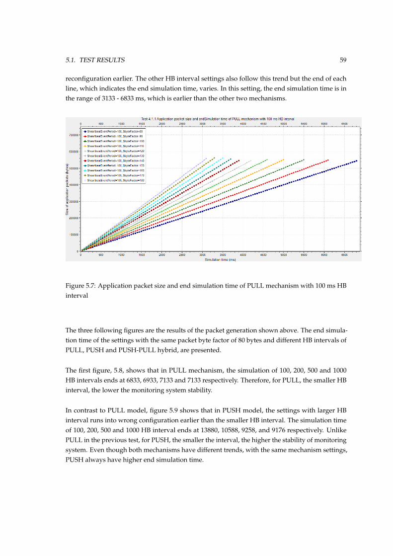
5.1. TEST RESULTS 59
reconfiguration earlier. The other HB interval settings also follow this trend but the end of eachline, which indicates the end simulation time, varies. In this setting, the end simulation time is inthe range of 3133 - 6833 ms, which is earlier than the other two mechanisms.
Figure 5.7: Application packet size and end simulation time of PULL mechanism with 100 ms HBinterval
The three following figures are the results of the packet generation shown above. The end simula-tion time of the settings with the same packet byte factor of 80 bytes and different HB intervals ofPULL, PUSH and PUSH-PULL hybrid, are presented.
The first figure, 5.8, shows that in PULL mechanism, the simulation of 100, 200, 500 and 1000HB intervals ends at 6833, 6933, 7133 and 7133 respectively. Therefore, for PULL, the smaller HBinterval, the lower the monitoring system stability.
In contrast to PULL model, figure 5.9 shows that in PUSH model, the settings with larger HBinterval runs into wrong configuration earlier than the smaller HB interval. The simulation timeof 100, 200, 500 and 1000 HB interval ends at 13880, 10588, 9258, and 9176 respectively. UnlikePULL in the previous test, for PUSH, the smaller the interval, the higher the stability of monitoringsystem. Even though both mechanisms have different trends, with the same mechanism settings,PUSH always have higher end simulation time.
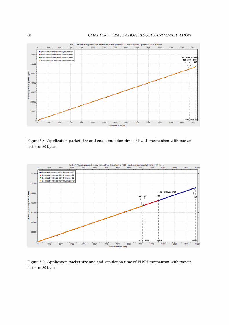
60 CHAPTER 5. SIMULATION RESULTS AND EVALUATION
Figure 5.8: Application packet size and end simulation time of PULL mechanism with packetfactor of 80 bytes
Figure 5.9: Application packet size and end simulation time of PUSH mechanism with packetfactor of 80 bytes
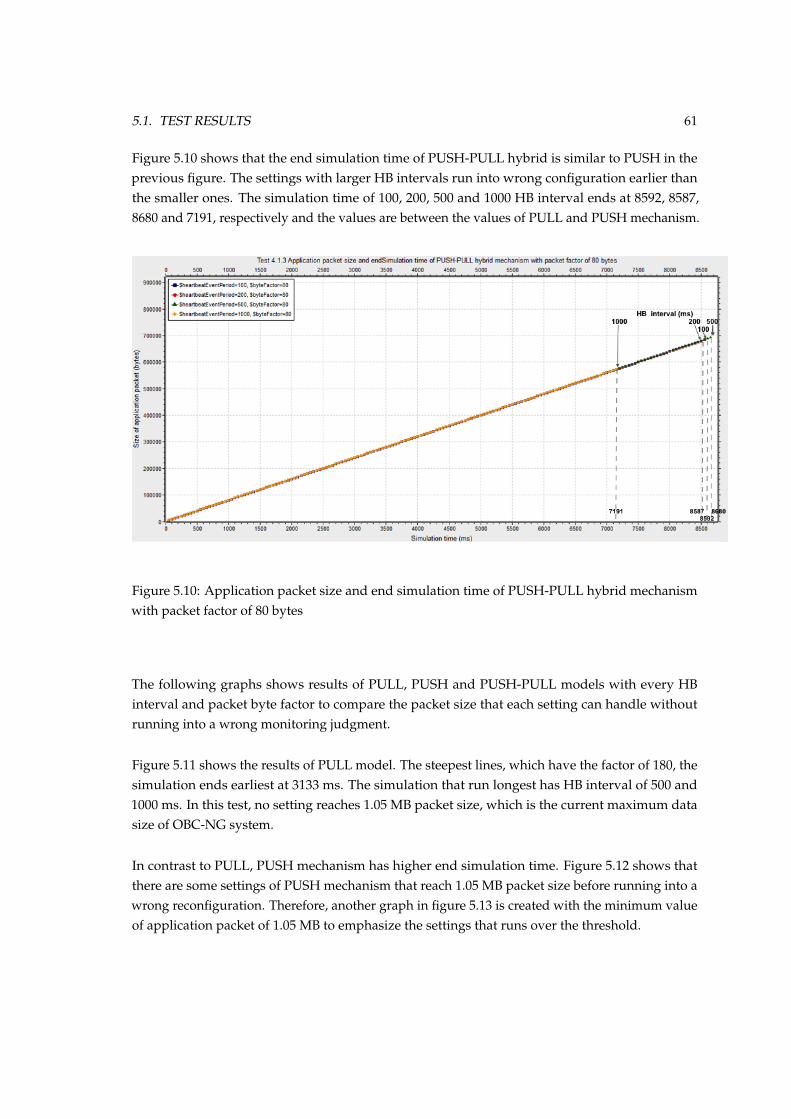
5.1. TEST RESULTS 61
Figure 5.10 shows that the end simulation time of PUSH-PULL hybrid is similar to PUSH in theprevious figure. The settings with larger HB intervals run into wrong configuration earlier thanthe smaller ones. The simulation time of 100, 200, 500 and 1000 HB interval ends at 8592, 8587,8680 and 7191, respectively and the values are between the values of PULL and PUSH mechanism.
Figure 5.10: Application packet size and end simulation time of PUSH-PULL hybrid mechanismwith packet factor of 80 bytes
The following graphs shows results of PULL, PUSH and PUSH-PULL models with every HBinterval and packet byte factor to compare the packet size that each setting can handle withoutrunning into a wrong monitoring judgment.
Figure 5.11 shows the results of PULL model. The steepest lines, which have the factor of 180, thesimulation ends earliest at 3133 ms. The simulation that run longest has HB interval of 500 and1000 ms. In this test, no setting reaches 1.05 MB packet size, which is the current maximum datasize of OBC-NG system.
In contrast to PULL, PUSH mechanism has higher end simulation time. Figure 5.12 shows thatthere are some settings of PUSH mechanism that reach 1.05 MB packet size before running into awrong reconfiguration. Therefore, another graph in figure 5.13 is created with the minimum valueof application packet of 1.05 MB to emphasize the settings that runs over the threshold.
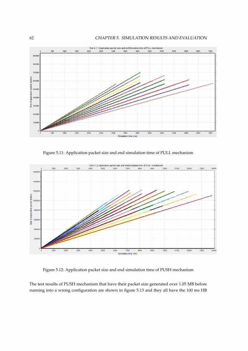
62 CHAPTER 5. SIMULATION RESULTS AND EVALUATION
Figure 5.11: Application packet size and end simulation time of PULL mechanism
Figure 5.12: Application packet size and end simulation time of PUSH mechanism
The test results of PUSH mechanism that have their packet size generated over 1.05 MB beforerunning into a wrong configuration are shown in figure 5.13 and they all have the 100 ms HB
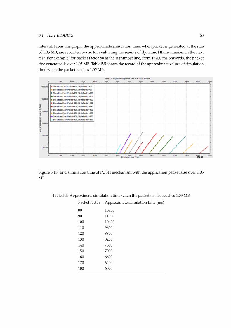
5.1. TEST RESULTS 63
interval. From this graph, the approximate simulation time, when packet is generated at the sizeof 1.05 MB, are recorded to use for evaluating the results of dynamic HB mechanism in the nexttest. For example, for packet factor 80 at the rightmost line, from 13200 ms onwards, the packetsize generated is over 1.05 MB. Table 5.5 shows the record of the approximate values of simulationtime when the packet reaches 1.05 MB.
Figure 5.13: End simulation time of PUSH mechanism with the application packet size over 1.05MB
Table 5.5: Approximate simulation time when the packet of size reaches 1.05 MB
Packet factor Approximate simulation time (ms)
80 1320090 11900100 10600110 9600120 8800130 8200140 7600150 7000160 6600170 6200180 6000
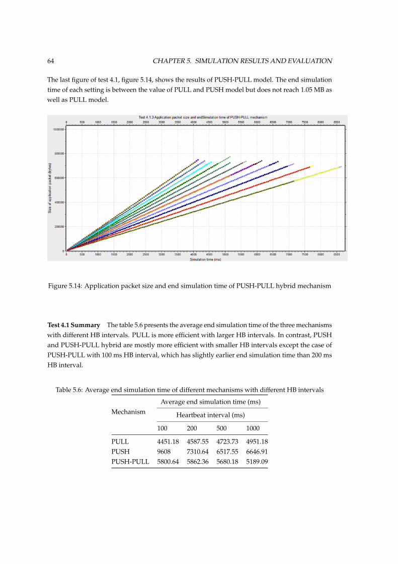
64 CHAPTER 5. SIMULATION RESULTS AND EVALUATION
The last figure of test 4.1, figure 5.14, shows the results of PUSH-PULL model. The end simulationtime of each setting is between the value of PULL and PUSH model but does not reach 1.05 MB aswell as PULL model.
Figure 5.14: Application packet size and end simulation time of PUSH-PULL hybrid mechanism
Test 4.1 Summary The table 5.6 presents the average end simulation time of the three mechanismswith different HB intervals. PULL is more efficient with larger HB intervals. In contrast, PUSHand PUSH-PULL hybrid are mostly more efficient with smaller HB intervals except the case ofPUSH-PULL with 100 ms HB interval, which has slightly earlier end simulation time than 200 msHB interval.
Table 5.6: Average end simulation time of different mechanisms with different HB intervals
MechanismAverage end simulation time (ms)
Heartbeat interval (ms)
100 200 500 1000
PULL 4451.18 4587.55 4723.73 4951.18PUSH 9608 7310.64 6517.55 6646.91PUSH-PULL 5800.64 5862.36 5680.18 5189.09
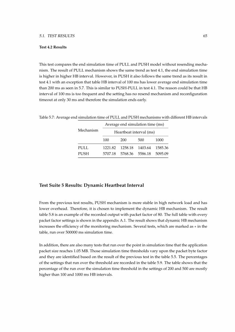
5.1. TEST RESULTS 65
Test 4.2 Results
This test compares the end simulation time of PULL and PUSH model without resending mecha-nism. The result of PULL mechanism shows the same trend as test 4.1, the end simulation timeis higher in higher HB interval. However, in PUSH it also follows the same trend as its result intest 4.1 with an exception that table HB interval of 100 ms has lower average end simulation timethan 200 ms as seen in 5.7. This is similar to PUSH-PULL in test 4.1. The reason could be that HBinterval of 100 ms is too frequent and the setting has no resend mechanism and reconfigurationtimeout at only 30 ms and therefore the simulation ends early.
Table 5.7: Average end simulation time of PULL and PUSH mechanisms with different HB intervals
MechanismAverage end simulation time (ms)
Heartbeat interval (ms)
100 200 500 1000
PULL 1221.82 1258.18 1403.64 1585.36PUSH 5707.18 5768.36 5586.18 5095.09
Test Suite 5 Results: Dynamic Heartbeat Interval
From the previous test results, PUSH mechanism is more stable in high network load and haslower overhead. Therefore, it is chosen to implement the dynamic HB mechanism. The resulttable 5.8 is an example of the recorded output with packet factor of 80. The full table with everypacket factor settings is shown in the appendix A.1. The result shows that dynamic HB mechanismincreases the efficiency of the monitoring mechanism. Several tests, which are marked as ⇤ in thetable, run over 500000 ms simulation time.
In addition, there are also many tests that run over the point in simulation time that the applicationpacket size reaches 1.05 MB. Those simulation time thresholds vary upon the packet byte factorand they are identified based on the result of the previous test in the table 5.5. The percentagesof the settings that run over the threshold are recorded in the table 5.9. The table shows that thepercentage of the run over the simulation time threshold in the settings of 200 and 500 are mostlyhigher than 100 and 1000 ms HB intervals.
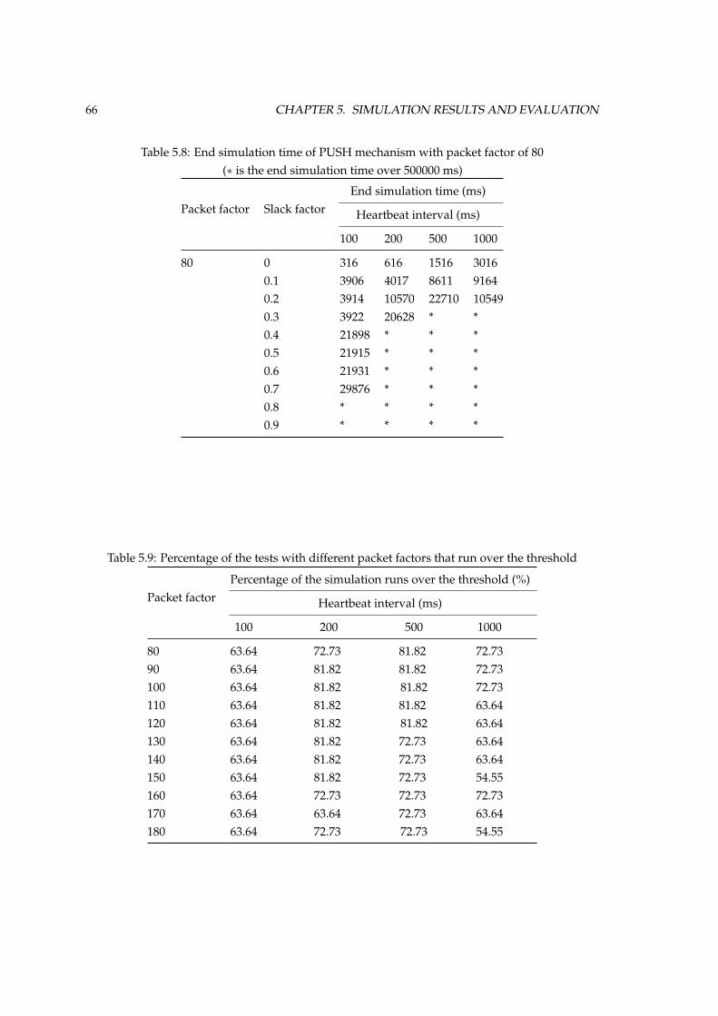
66 CHAPTER 5. SIMULATION RESULTS AND EVALUATION
Table 5.8: End simulation time of PUSH mechanism with packet factor of 80(⇤ is the end simulation time over 500000 ms)
Packet factor Slack factorEnd simulation time (ms)
Heartbeat interval (ms)
100 200 500 1000
80 0 316 616 1516 30160.1 3906 4017 8611 91640.2 3914 10570 22710 105490.3 3922 20628 * *0.4 21898 * * *0.5 21915 * * *0.6 21931 * * *0.7 29876 * * *0.8 * * * *0.9 * * * *
Table 5.9: Percentage of the tests with different packet factors that run over the threshold
Packet factorPercentage of the simulation runs over the threshold (%)
Heartbeat interval (ms)
100 200 500 1000
80 63.64 72.73 81.82 72.7390 63.64 81.82 81.82 72.73100 63.64 81.82 81.82 72.73110 63.64 81.82 81.82 63.64120 63.64 81.82 81.82 63.64130 63.64 81.82 72.73 63.64140 63.64 81.82 72.73 63.64150 63.64 81.82 72.73 54.55160 63.64 72.73 72.73 72.73170 63.64 63.64 72.73 63.64180 63.64 72.73 72.73 54.55
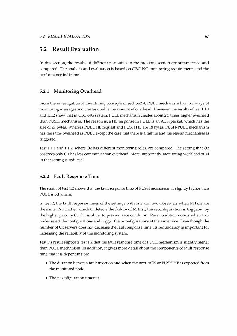
5.2. RESULT EVALUATION 67
5.2 Result Evaluation
In this section, the results of different test suites in the previous section are summarized andcompared. The analysis and evaluation is based on OBC-NG monitoring requirements and theperformance indicators.
5.2.1 Monitoring Overhead
From the investigation of monitoring concepts in section2.4, PULL mechanism has two ways ofmonitoring messages and creates double the amount of overhead. However, the results of test 1.1.1and 1.1.2 show that in OBC-NG system, PULL mechanism creates about 2.5 times higher overheadthan PUSH mechanism. The reason is, a HB response in PULL is an ACK packet, which has thesize of 27 bytes. Whereas PULL HB request and PUSH HB are 18 bytes. PUSH-PULL mechanismhas the same overhead as PULL except the case that there is a failure and the resend mechanism istriggered.
Test 1.1.1 and 1.1.2, where O2 has different monitoring roles, are compared. The setting that O2observes only O1 has less communication overhead. More importantly, monitoring workload of Min that setting is reduced.
5.2.2 Fault Response Time
The result of test 1.2 shows that the fault response time of PUSH mechanism is slightly higher thanPULL mechanism.
In test 2, the fault response times of the settings with one and two Observers when M fails arethe same. No matter which O detects the failure of M first, the reconfiguration is triggered bythe higher priority O, if it is alive, to prevent race condition. Race condition occurs when twonodes select the configurations and trigger the reconfigurations at the same time. Even though thenumber of Observers does not decrease the fault response time, its redundancy is important forincreasing the reliability of the monitoring system.
Test 3’s result supports test 1.2 that the fault response time of PUSH mechanism is slightly higherthan PULL mechanism. In addition, it gives more detail about the components of fault responsetime that it is depending on:
• The duration between fault injection and when the next ACK or PUSH HB is expected fromthe monitored node.
• The reconfiguration timeout
68 CHAPTER 5. SIMULATION RESULTS AND EVALUATION
• Network latency to deliver the reconfiguration, error notification, HB and ACK messages.This is depending on the number of hops between the monitor and the monitored node.
Minimum value of fault response time is from the case that the fault injection occurs right at thetime when a HB or an ACK is expected to be sent out. Therefore, the value is the reconfigurationtimeout plus the network latency. Maximum value, however, includes the time from the failure tothe first reconfiguration is finished if the failure occur before it is finished. The duration is added tothe value of full HB interval + reconfiguration timeout + network latency, which is the case whenfault injection occurs right after the time a HB or an ACK is sent. The range between maximumand minimum varies upon the HB interval.
Heartbeat Interval and Reconfiguration Timeout The settings with smaller HB interval, whichhave higher HB frequency, allow the missing HB to be detected earlier. The reconfiguration timeoutneeds to be set up to make sure the monitored node has failed to sent a HB. If the reconfigurationtimeout is too short, the risk of misinterpreting a delayed HB as a node failure is higher. However,if the reconfiguration timeout is longer, the fault response time increases.
However, small HB intervals are not suitable for PULL mechanism since the monitoring messagesare in two ways (request and response) so it has higher risk of losing one of the messages.
The previous assumption of PUSH mechanism was that the resend mechanism cannot be imple-mented and in order to implement it, the monitoring systems have to switch to PULL mechanism.However, the HB interval and reconfiguration timeout of PUSH mechanism can be set up in a waythat it waits for the same amount of PUSH HB as the resend threshold. For example, with 100 msHB interval, and 400 ms reconfiguration timeout. After a missing HB, the monitored node passesthree HB intervals before the reconfiguration is triggered.
5.2.3 Monitoring System Stability
In test 4, network traffic is generated to test the monitoring system stability. For static HB interval,different mechanisms with the same reconfiguration timeout of 120 ms have different the endsimulation time. The result of test 4.1 shows that PULL tends to run into a wrong configurationand end the simulation earliest because of its two ways of communication. PUSH mechanism hasthe higher end simulation time because it has one way of monitoring message and PUSH-PULLis in the middle because in the end, PULL is implemented as a resend mechanism. To analyzethe mechanisms, PULL and PUSH mechanism without resend mechanisms are simulated in test4.2 and the results confirm that PUSH mechanism is more stable than PULL, when there is highnetwork load.
HB interval settings affect the stability differently. From test 4.1 and 4.2, PULL is more stable withthe larger HB intervals and PUSH is more stable with the smaller intervals.

5.2. RESULT EVALUATION 69
The results of dynamic HB interval mechanism in test 5 show that it increases the stability of everymechanism settings. However, 100 and 1000 ms HB interval shows lower efficiency than 200 and500. The result of 100 ms HB interval supports the observation grade-heartbeat (dynamic HB)experiment in subsection 2.4.3 that, frequent changes in HB interval result in the decline of themonitoring system efficiency. In the case of 1000 ms HB interval, the adjustment is not frequentenough when packet factor is high and the application packet size increases steeply.

Chapter 6
Conclusion and Future Work
In this work, various monitoring mechanisms of distributed system are investigated to designthe monitoring system of OBC-NG. Three mechanisms, PULL, PUSH and PUSH-PULL hybrid,are chosen to be tested and analyzed to find the one that has high efficiency, low overhead andhigh stability. The monitoring mechanism testing is divided into five test suites and the concludedresults are shown in section 6.1. Finally, section 6.2 presents the future outlook how the designsand the results could be used for the further development of the OBC-NG system.
6.1 Final Results
Monitoring Mechanism
PULL, PUSH and PUSH-PULL mechanisms are tested with different mechanism settings andenvironment settings to compare the monitoring efficiency, overhead and stability. The monitoringmodels have been evaluated base on the OBC-NG monitoring requirements.
The monitoring mechanisms and mechanism settings have been analyzed as follows: The currentlyimplemented model of PULL has the highest monitoring workload on M and the highest networkoverhead. Adjusting the role of Observer setting decreases the workload on the M, but themonitoring network load is still higher than in the other two mechanisms.
PUSH mechanism has the lowest monitoring overhead, 2.5 times lower than PULL. Its faultresponse time is slightly higher than PULL but it has a lot higher stability of the monitoring, whenthere is high network load.
71
72 CHAPTER 6. CONCLUSION AND FUTURE WORK
Mechanism Settings
The higher number of Observers does not affect the fault response time but the reliability. TheHB interval should be set differently according to the mechanism. Larger HB intervals are moreefficient in PULL model and smaller intervals are better in PUSH and PUSH-PULL models. Theresults show the range of the fault response time of each HB interval. However, the exact valueof a HB interval should be mission-specifically configured, using the range of the fault responsetime measured from the test and in the mission requirements. Lastly, the higher reconfigurationtimeout decreases the probability of false monitoring judgment without the requirement of resendmechanism.
Dynamic Heartbeat Mechanism
Base on the test results mentioned above, PUSH has been chosen for implementing dynamic HBmechanism. The mechanism increases the stability of every HB interval setting and decreasesthe false monitoring judgment. However, the default value of HB interval at the beginning andthe slack factor, to calculate the next interval, are important. If the HB interval is too short, themonitoring efficiency decreases because the frequency of the HB interval adjustments is high. Incontrast to that, if the HB interval is too long, the HB interval adjustments are not frequent enough,in case of high network traffic in the system. Therefore, the HB frequency and slack factor shouldbe chosen base on the maximum size of packets and the assumption of the frequency of applicationpackets.
6.2 Future Work
In the future, PUSH mechanism, which is selected in the final results as the most efficient mecha-nism can be integrated in the Scalable on-board Computing for Space Avionics (ScOSA) project.This project is the successor of the OBC-NG and has similar design. It is also a distributed, scalablesystem with interconnected nodes, whereas nodes can be COTS as well as radiation-hardenedcomponents.
The traffic sensing mechanism of PUSH dynamic HB, which is used for adjusting the watchdogtimer, implicitly informs the M about the current traffic load on the network. This enables the M toinform other W nodes that they shall prioritize their output on the network. To derive a correctverdict, the M needs to be positioned near or in the center of the network.
Heartbeat monitoring used in this work is a mechanism for implicit monitoring and the failureis detected by the monitor. In the future, explicit monitoring can be integrated in the form of anagent-based system, in which an application can use an agent service on the node to inform the M
6.2. FUTURE WORK 73
and the monitoring system about a certain inconsistency. The M and the monitoring system thenmight have more time to evaluate the system health and to react in case required.
Moreover, the functionality of the monitor can be increased to evaluate the system health status,in case a missing HB or other negative symptoms are sensed. After a missing HB, during thereconfiguration timeout, the monitor has the possibility to prepare itself and the other nodes into apre-reconfiguration state. Tasks, such as searching for the next configuration in the decision tree andthe pre-distribution of checkpoint values for warm redundancy, can be conducted.
When a reconfiguration has to be triggered, the current mechanism reconfigures the entire systemincluding the healthy nodes. In the future, partial reconfiguration can be designed to isolate thefailed node and redistributing its tasks without interrupting the tasks of the healthy nodes.
Furthermore, monitoring can be conducted in a finer grained level, such as task level, instead ofnode level. When a failure occurs, a specific task is migrated to another node instead of migratingall the tasks. This requires a more detailed knowledge of the monitoring system, regarding thefaults, which can be provided by a more sophisticated error messaging.

Bibliography
[1] D. P. Siewiorek and P. Narasimhan, “Fault-tolerant architectures for space and avionicsapplications,” electrical and Computer Engineering Department Carnegie Mellon University.
[2] D. Lüdtke, K. Westerdorff, K. Stohlmann, A. Börner, O. Maibaum, T.Peng, B. Weps, G. Fey,and A. Gerndt, “OBC-NG: Towards a reconfigurable on-board computing architecture forspacecraft,” in 2014 IEEE Aerospace Conference, 2014, pp. 1–13.
[3] S. Parkes, SpaceWire User’s Guide. STAR-Dundee Limited, 2012.
[4] H. Kopetz, Real-Time Systems Design Principles for Distributed Embedded Applications, 2nd ed.Springer US, 2011.
[5] G. A. Klutke, P. C. Kiessler, and M. A. Wortman, “A critical look at the bathtub curve,” IEEETransactions on Reliability, vol. 52, no. 1, pp. 125–129, March 2003.
[6] M. Mansouri-Samani and M. Sloman, “Network and distributed systems management,”M. Sloman, Ed. Boston, MA, USA: Addison-Wesley Longman Publishing Co.,Inc., 1994, ch. Monitoring Distributed Systems, pp. 303–347. [Online]. Available:http://dl.acm.org/citation.cfm?id=184430.184469
[7] M. Technet. (2016) How heartbeats work in operations manager. [Online]. Available:https://technet.microsoft.com/en-us/library/hh212798.aspx
[8] Y. Wan, D. Feng, T. Yang, Z. Deng, and L. Liu, “The adaptive heartbeat design of highavailability raid dual-controller,” in Multimedia and Ubiquitous Engineering, 2008. MUE 2008.International Conference on, April 2008, pp. 45–50.
[9] S. W. Heinen, S. Reid, “Automation through on-board control procedures: Operationalconcepts and tools,” american Institute of Aeronautics and Astronautics.
[10] M. Lauer, U. Herfort, D. Hocken, and S. Kielbassa, “Optical measurements for the flybynavigation of rosetta at asteroid steins,” in Proceedings 21st International Symposium on SpaceFlight Dynamics–21st ISSFD. Toulouse, France, 2009.
75
76 BIBLIOGRAPHY
[11] T. Peng, K. Höflinger, B. Weps, O. Maibaum, K. Schwenk, D. Lüdtke, and A. Gerndt, “AComponent-Based Middleware for a Reliable Distributed and Reconfigurable SpacecraftOnboard Computer,” in 35th Symposium on Reliable Distributed Systems (SRDS).
[12] S. M. Parkes and P. Armbruster, “Spacewire: a spacecraft onboard network for real-timecommunications,” in 14th IEEE-NPSS Real Time Conference, 2005., June 2005, pp. 6–10.
[13] S. Parkes, Supporting SpaceWire Applications, STAR-Dundee Ltd, School of Computing, Univer-sity of Dundee Dundee, DD1 4HN, Scotland, UK.
[14] A. Hamed and K. Jaber, “Analysis of quality of service in cloud storage systems,” IJFCSTInternational Journal in Foundations of Computer Science Technology, vol. 4, no. 6, p. 71–77, 2014.
[15] S. Kapurch, NASA Systems Engineering Handbook. DIANE Publishing Company, 2010.[Online]. Available: https://books.google.de/books?id=2CDrawe5AvEC
[16] M. Kooli and G. D. Natale, “A survey on simulation-based fault injection tools for complexsystems,” in Design Technology of Integrated Systems In Nanoscale Era (DTIS), 2014 9th IEEEInternational Conference On, May 2014, pp. 1–6.
[17] I. Eusgeld, F. Freiling, and R. Reussner, Dependability Metrics: GI-Dagstuhl ResearchSeminar, Dagstuhl Castle, Germany, October 5 - November 1, 2005, Advanced Lectures, ser.Lecture Notes in Computer Science. Springer Berlin Heidelberg, 2008. [Online]. Available:https://books.google.de/books?id=HX5rCQAAQBAJ
[18] J. Azambuja, F. Kastensmidt, and J. Becker, Hybrid Fault Tolerance Techniques to Detect TransientFaults in Embedded Processors, ser. SpringerLink : Bücher. Springer International Publishing,2014. [Online]. Available: https://books.google.de/books?id=b1clBAAAQBAJ
[19] D.-M. Kwai and B. Parhami, “Fault-tolerant processor arrays using space and time redun-dancy,” in Algorithms amp; Architectures for Parallel Processing, 1996. ICAPP 96. 1996 IEEESecond International Conference on, Jun 1996, pp. 303–310.
[20] NASA. Mean time to repair predictions. [Online]. Available: http://llis.nasa.gov/lesson/840
[21] J. Joyce, G. Lomow, K. Slind, and B. Unger, “Monitoring distributed systems,” ACMTrans. Comput. Syst., vol. 5, no. 2, pp. 121–150, Mar. 1987. [Online]. Available:http://doi.acm.org/10.1145/13677.22723
[22] C.-f. Hsin and M. Liu, “A distributed monitoring mechanism for wireless sensor networks,”in Proceedings of the 1st ACM Workshop on Wireless Security, ser. WiSE ’02. New York, NY,USA: ACM, 2002, pp. 57–66. [Online]. Available: http://doi.acm.org/10.1145/570681.570688
[23] J. X. Zou, Z. Q. Zhang, and H. B. Xu, “Design of heartbeat invalidation detecting mecha-nism in triple module redundant multi-machine system,” in 2009 IEEE Circuits and SystemsInternational Conference on Testing and Diagnosis, April 2009, pp. 1–4.
BIBLIOGRAPHY 77
[24] F. V. Brasileiro, P. D. Ezhilchelvan, S. K. Shrivastava, N. A. Speirs, and S. Tao, “Implementingfail-silent nodes for distributed systems,” IEEE Transactions on Computers, vol. 45, no. 11, pp.1226–1238, Nov 1996.
[25] B. Satzger, A. Pietzowski, W. Trumler, and T. Ungerer, “A lazy monitoring approach forheartbeat-style failure detectors,” in Availability, Reliability and Security, 2008. ARES 08. ThirdInternational Conference on, March 2008, pp. 404–409.
[26] K. Rachuri, A. A. Franklin, and C. S. R. Murthy, Coverage Based Expanding Ring Search forDense Wireless Sensor Networks. Berlin, Heidelberg: Springer Berlin Heidelberg, 2008, pp.245–256. [Online]. Available: http://dx.doi.org/10.1007/978-3-540-89894-8_24
[27] H. Huang and L. Wang, “P amp;p: A combined push-pull model for resource monitoring incloud computing environment,” in 2010 IEEE 3rd International Conference on Cloud Computing,July 2010, pp. 260–267.
[28] Y. Zhao, “A model of computation with push and pull processing,” Technical MemorandumElectronics Research Laboratory University of California at Berkeley, dec 2003.
[29] A. Vargas, “Omnet++ user guide version 4.6,” 2014.
[30] A. Varga and R. Hornig, “An overview of the omnet++ simulation environment,”in Proceedings of the 1st International Conference on Simulation Tools and Techniquesfor Communications, Networks and Systems & Workshops, ser. Simutools ’08. ICST,Brussels, Belgium, Belgium: ICST (Institute for Computer Sciences, Social-Informaticsand Telecommunications Engineering), 2008, pp. 60:1–60:10. [Online]. Available: http://dl.acm.org/citation.cfm?id=1416222.1416290

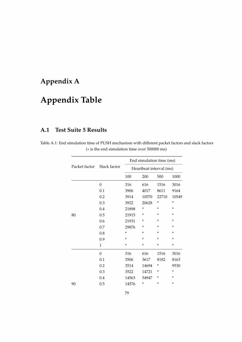
Appendix A
Appendix Table
A.1 Test Suite 5 Results
Table A.1: End simulation time of PUSH mechanism with different packet factors and slack factors(⇤ is the end simulation time over 500000 ms)
Packet factor Slack factorEnd simulation time (ms)
Heartbeat interval (ms)
100 200 500 1000
80
0 316 616 1516 30160.1 3906 4017 8611 91640.2 3914 10570 22710 105490.3 3922 20628 * *0.4 21898 * * *0.5 21915 * * *0.6 21931 * * *0.7 29876 * * *0.8 * * * *0.9 * * * *1 * * * *
90
0 316 616 1516 30160.1 3506 3617 8182 81630.2 3514 14694 * 95300.3 3522 14721 * *0.4 14563 54947 * *0.5 14576 * * *
79
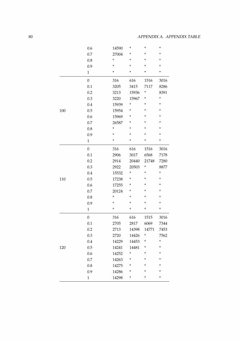
80 APPENDIX A. APPENDIX TABLE
0.6 14590 * * *0.7 27004 * * *0.8 * * * *0.9 * * * *1 * * * *
100
0 316 616 1516 30160.1 3205 3415 7117 82860.2 3213 15936 * 83910.3 3220 15967 * *0.4 15939 * * *0.5 15954 * * *0.6 15969 * * *0.7 26587 * * *0.8 * * * *0.9 * * * *1 * * * *
110
0 316 616 1516 30160.1 2906 3017 6568 71780.2 2914 20440 21748 72800.3 2922 20503 * 88770.4 15532 * * *0.5 17238 * * *0.6 17255 * * *0.7 20124 * * *0.8 * * * *0.9 * * * *1 * * * *
120
0 316 616 1515 30160.1 2705 2817 6069 73440.2 2713 14398 14771 74530.3 2720 14426 * 75620.4 14229 14453 * *0.5 14241 14481 * *0.6 14252 * * *0.7 14263 * * *0.8 14275 * * *0.9 14286 * * *1 14298 * * *
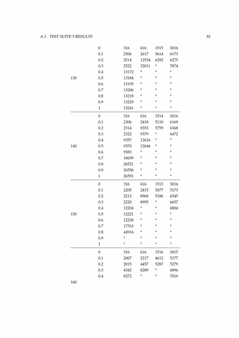
A.1. TEST SUITE 5 RESULTS 81
130
0 316 616 1515 30160.1 2506 2617 5614 61730.2 2514 12534 6292 62750.3 2522 32011 * 78740.4 13172 * * *0.5 13184 * * *0.6 13195 * * *0.7 13206 * * *0.8 13218 * * *0.9 13229 * * *1 13241 * * *
140
0 316 616 1514 30160.1 2306 2418 5110 61690.2 2314 9353 5759 63680.3 2322 9379 * 64720.4 9357 12616 * *0.5 9370 12644 * *0.6 9383 * * *0.7 18659 * * *0.8 26521 * * *0.9 26556 * * *1 26591 * * *
150
0 316 616 1513 30160.1 2205 2415 5077 51730.2 2213 8968 5186 65450.3 2220 8995 * 66570.4 12204 * * 68040.5 12221 * * *0.6 12238 * * *0.7 17763 * * *0.8 44916 * * *0.9 * * * *1 * * * *
160
0 316 616 1516 30150.1 2007 2217 4612 51770.2 2015 4457 5287 52790.3 4342 8289 * 68960.4 8272 * * 7019
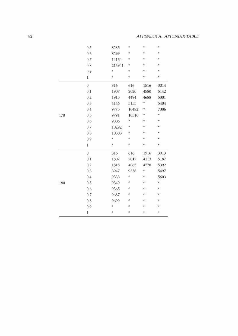
82 APPENDIX A. APPENDIX TABLE
0.5 8285 * * *0.6 8299 * * *0.7 14134 * * *0.8 213941 * * *0.9 * * * *1 * * * *
170
0 316 616 1516 30140.1 1907 2020 4580 51420.2 1915 4494 4688 53010.3 4146 5155 * 54040.4 9775 10482 * 73860.5 9791 10510 * *0.6 9806 * * *0.7 10292 * * *0.8 10303 * * *0.9 * * * *1 * * * *
180
0 316 616 1516 30130.1 1807 2017 4113 51870.2 1815 4065 4778 53920.3 3947 9358 * 54970.4 9333 * * 56030.5 9349 * * *0.6 9365 * * *0.7 9687 * * *0.8 9699 * * *0.9 * * * *1 * * * *