Embed Size (px)
Citation preview
Monitoring in the Ahupua‘a
Michael Tomlinson
Department of Oceanography
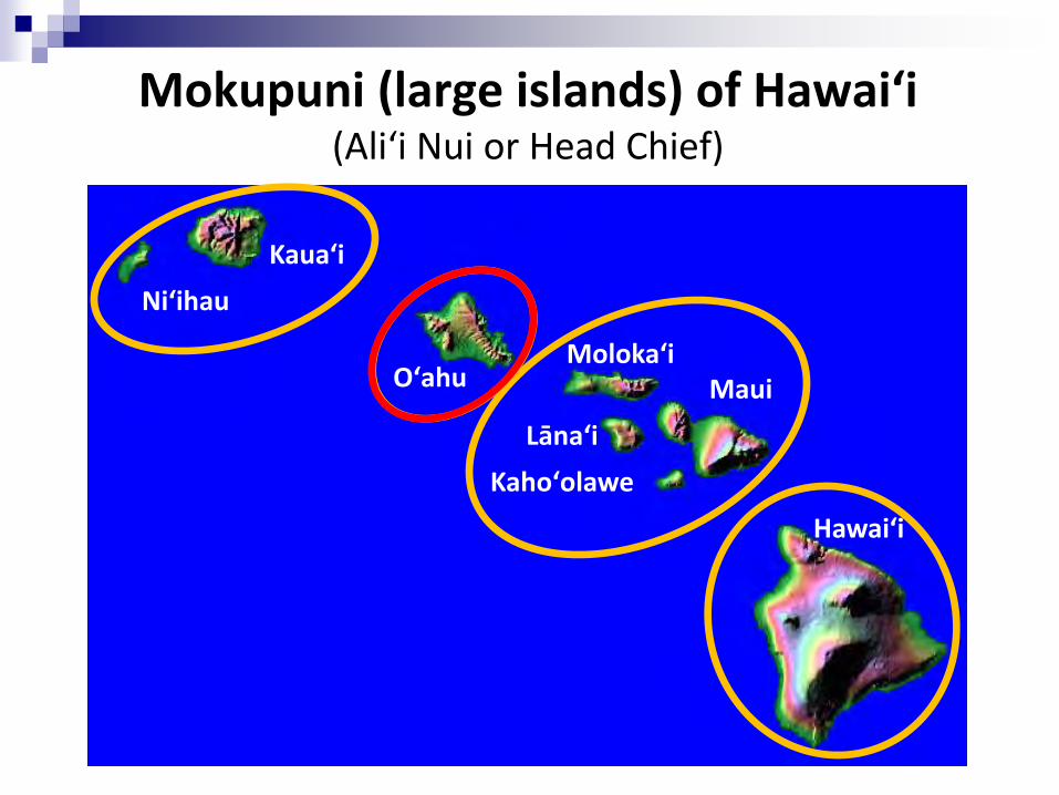
Mokupuni (large islands) of Hawaiʻi (Aliʻi Nui or Head Chief)
Kauaʻi
Niʻihau
Kahoʻolawe
Lānaʻi
Molokaʻi Maui
Hawaiʻi
Oʻahu
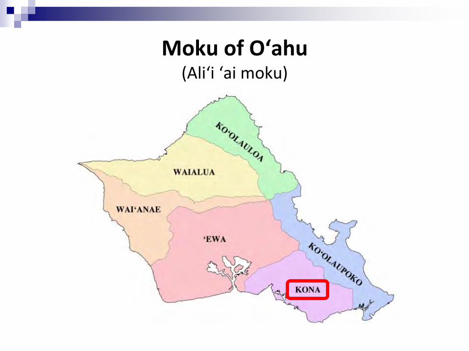
Moku of Oʻahu (Aliʻi ʻai moku)
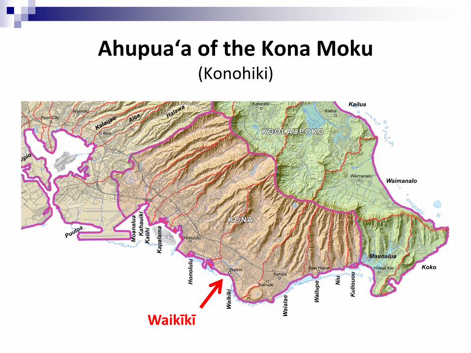
Ahupuaʻa of the Kona Moku (Konohiki)
Waikīkī
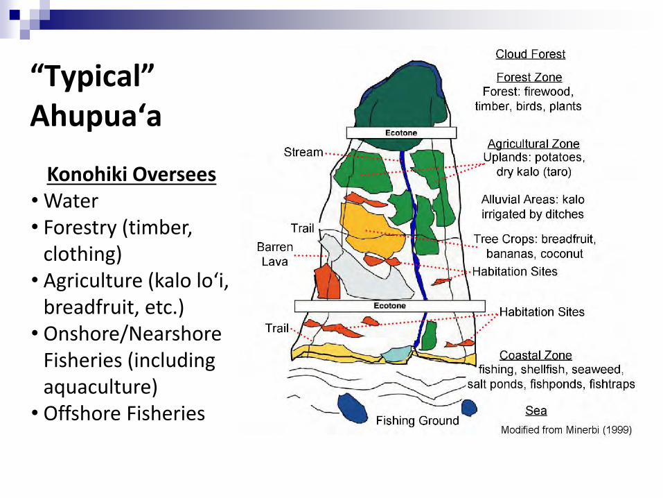
“Typical” Ahupua‘a
Konohiki Oversees • Water • Forestry (timber,
clothing) • Agriculture (kalo loʻi,
breadfruit, etc.) • Onshore/Nearshore
Fisheries (including aquaculture)
• Offshore Fisheries
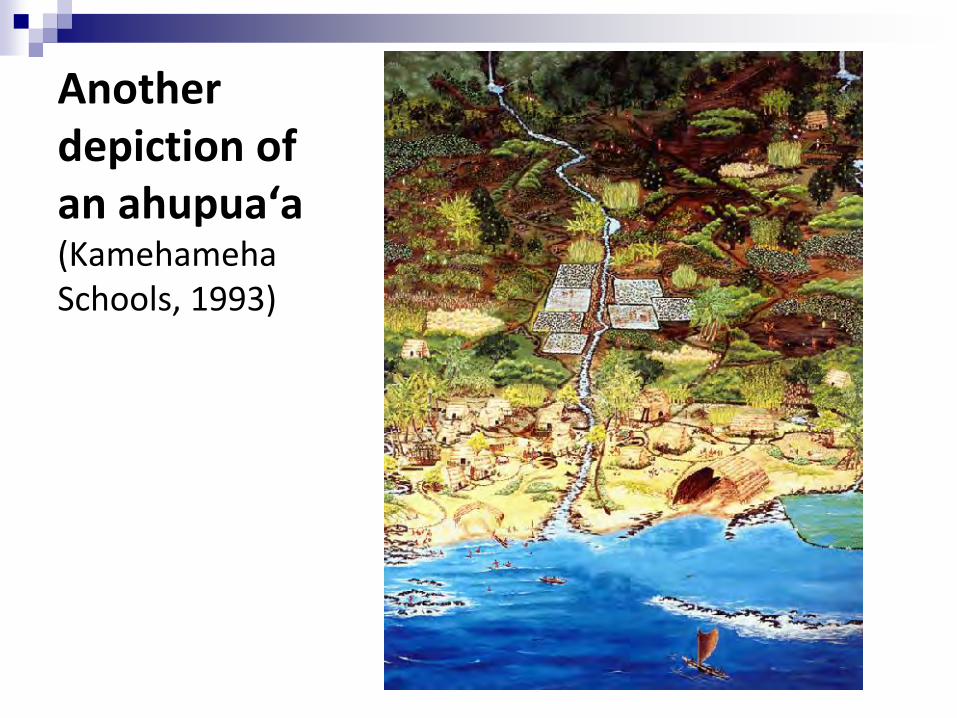
Another depiction of an ahupuaʻa (Kamehameha Schools, 1993)
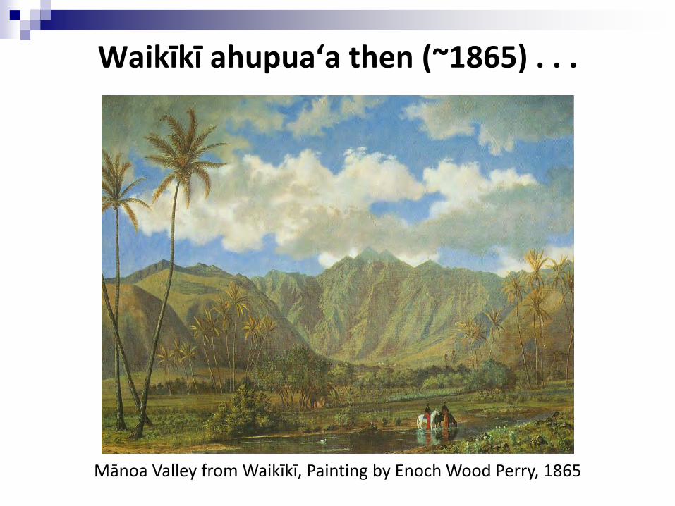
Waikīkī ahupuaʻa then (~1865) . . .
Mānoa Valley from Waikīkī, Painting by Enoch Wood Perry, 1865
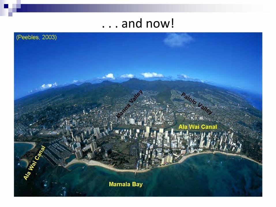
. . . and now!
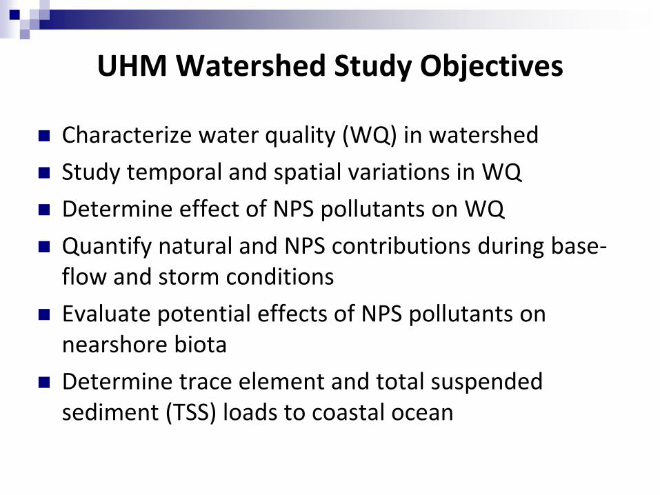
Characterize water quality (WQ) in watershed
Study temporal and spatial variations in WQ
Determine effect of NPS pollutants on WQ
Quantify natural and NPS contributions during base-flow and storm conditions
Evaluate potential effects of NPS pollutants on nearshore biota
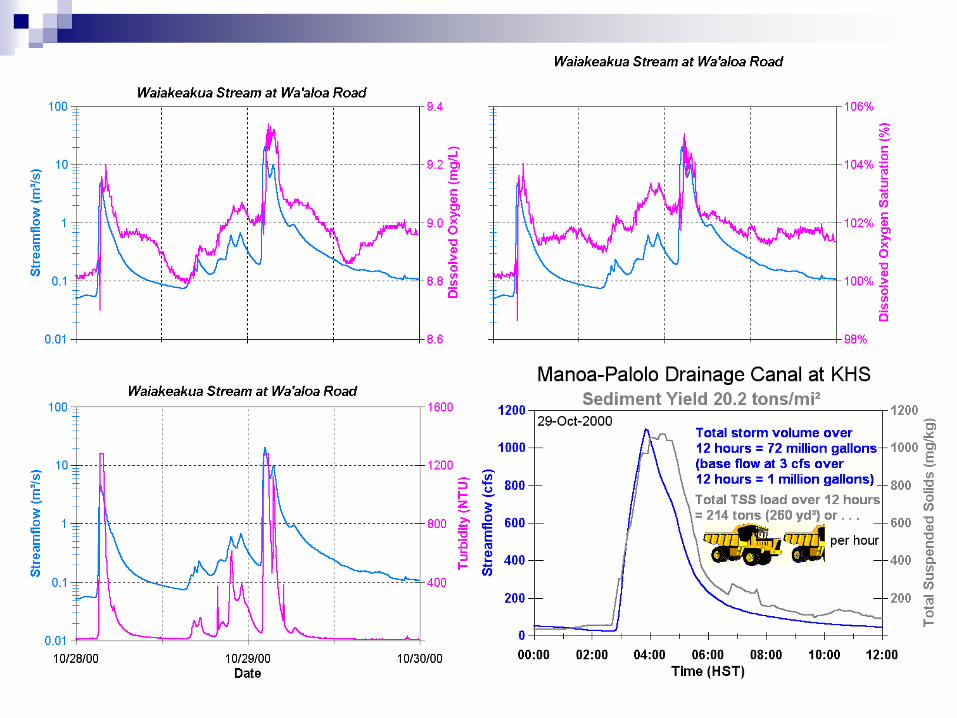
Determine trace element and total suspended sediment (TSS) loads to coastal ocean
UHM Watershed Study Objectives
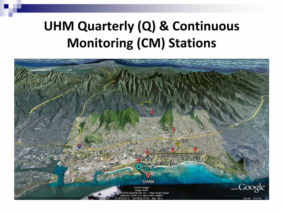
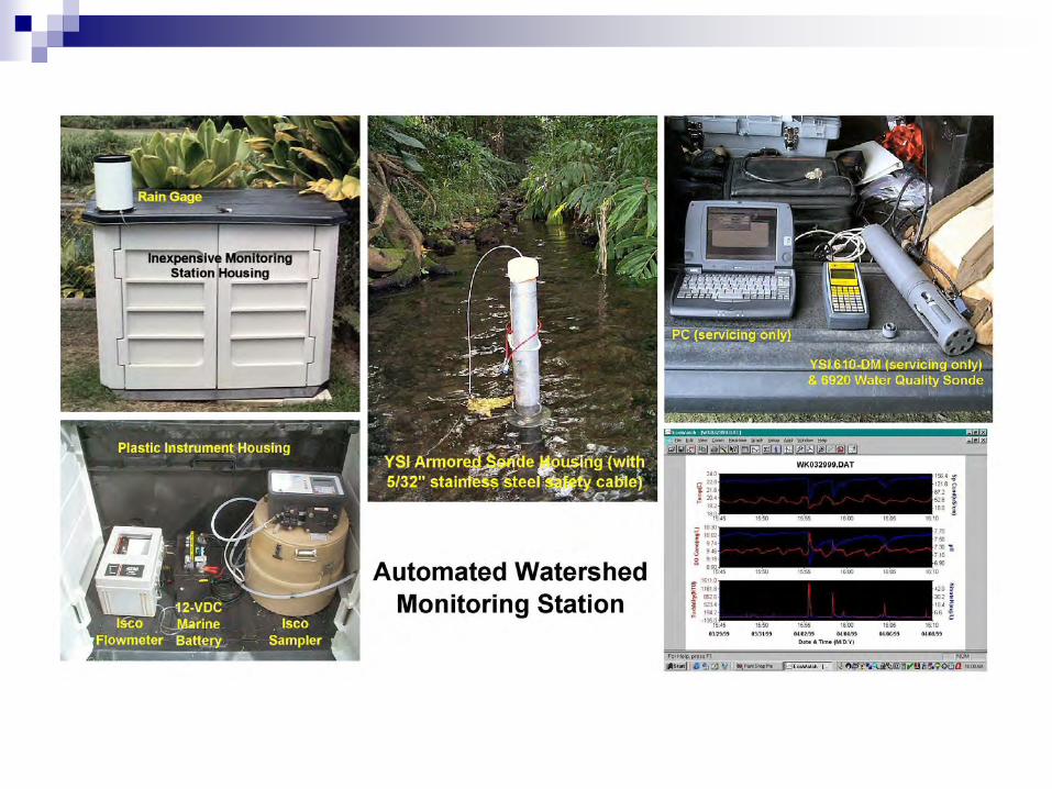
UHM Quarterly (Q) & Continuous Monitoring (CM) Stations
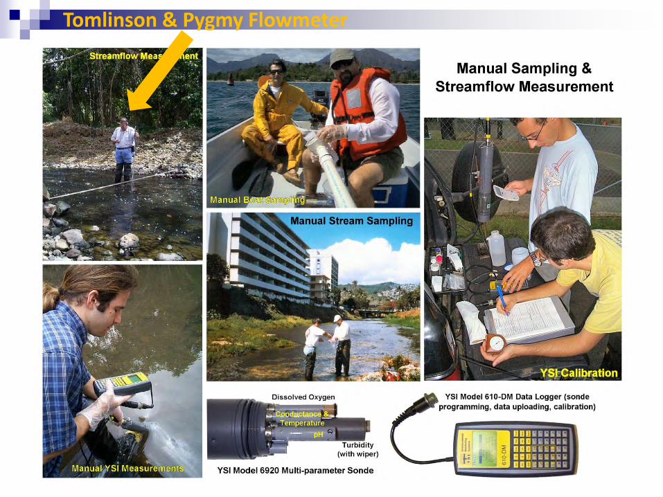
Tomlinson & Pygmy Flowmeter
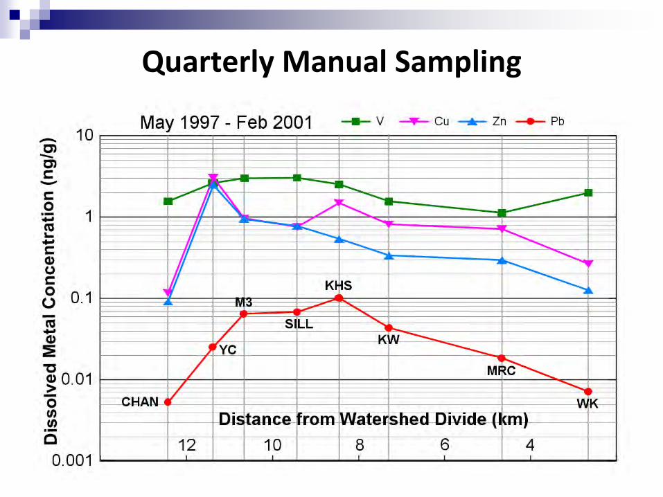
Quarterly Manual Sampling
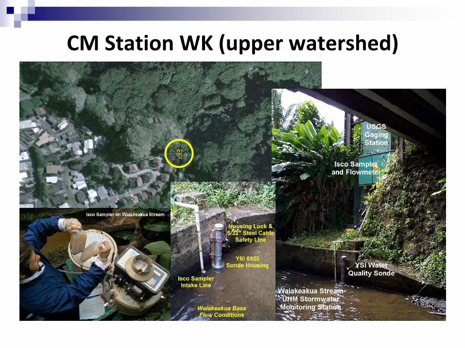
CM Station WK (upper watershed)
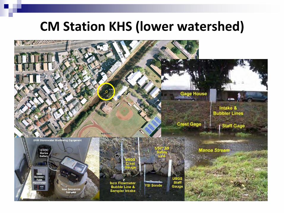
CM Station KHS (lower watershed)
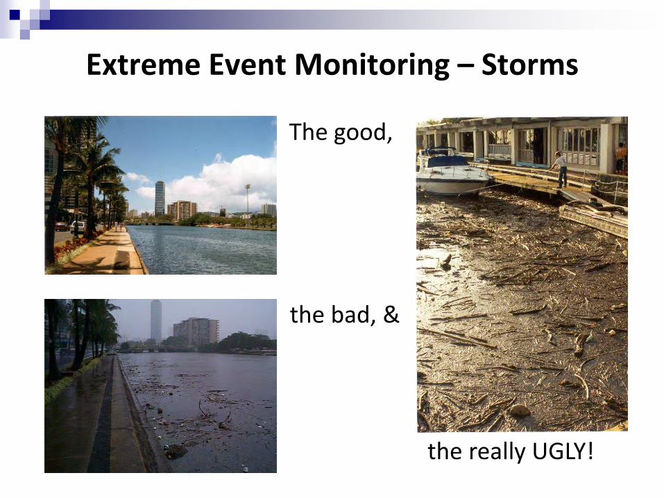
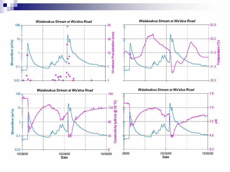
Extreme Event Monitoring – Storms
The good,
the bad, &
the really UGLY!
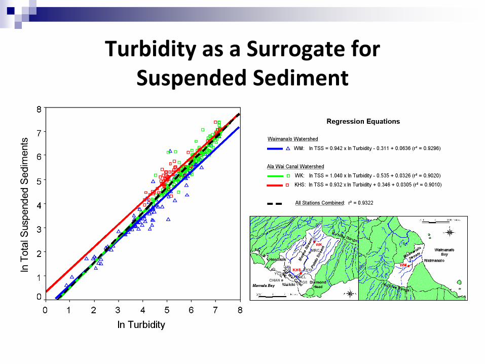
Turbidity as a Surrogate for Suspended Sediment
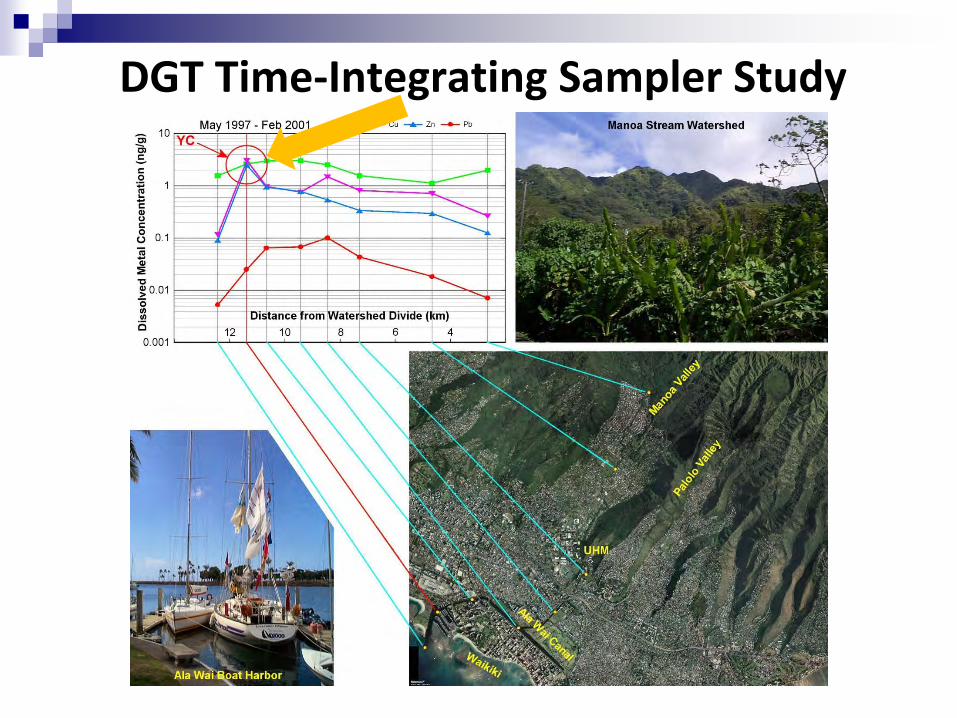
DGT Time-Integrating Sampler Study
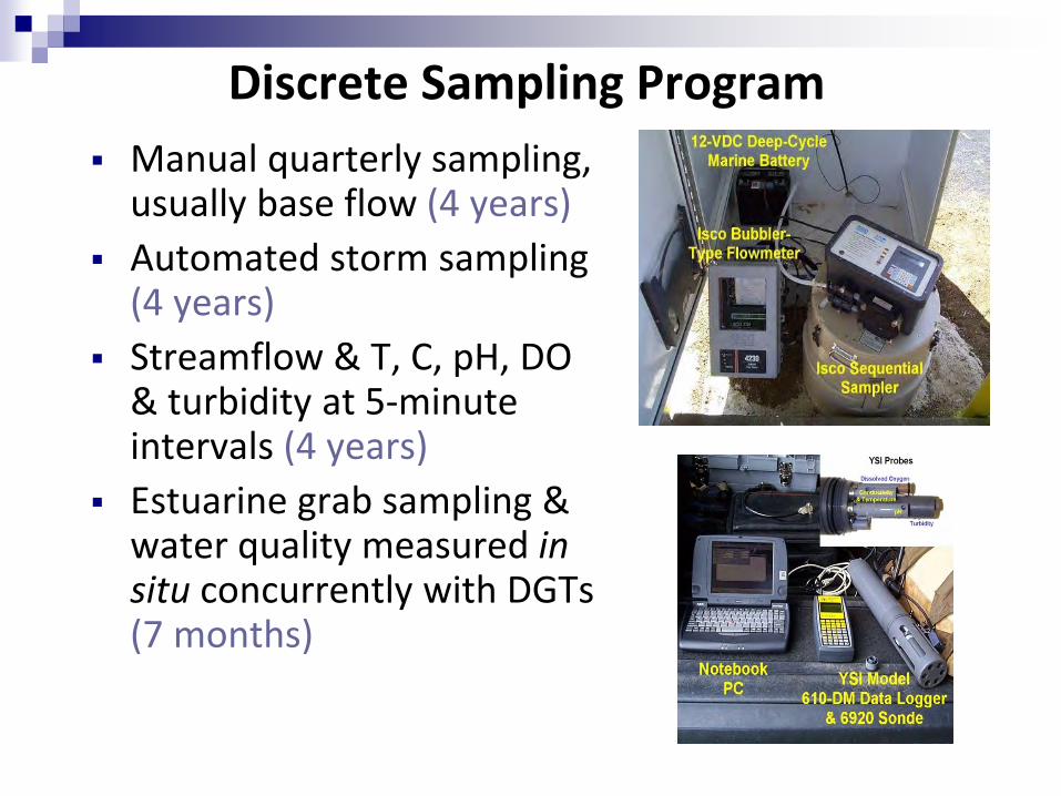
Discrete Sampling Program
Manual quarterly sampling, usually base flow (4 years)
Automated storm sampling (4 years)
Streamflow & T, C, pH, DO & turbidity at 5-minute intervals (4 years)
Estuarine grab sampling & water quality measured in situ concurrently with DGTs (7 months)
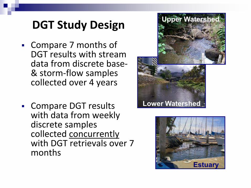
DGT Study Design
Compare 7 months of DGT results with stream data from discrete base- & storm-flow samples collected over 4 years
Compare DGT results with data from weekly discrete samples collected concurrently with DGT retrievals over 7 months
Estuary
Lower Watershed
Upper Watershed
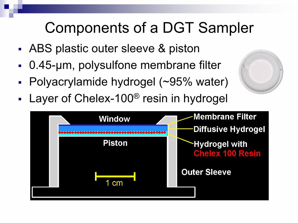
Components of a DGT Sampler ABS plastic outer sleeve & piston 0.45-µm, polysulfone membrane filter Polyacrylamide hydrogel (~95% water) Layer of Chelex-100® resin in hydrogel
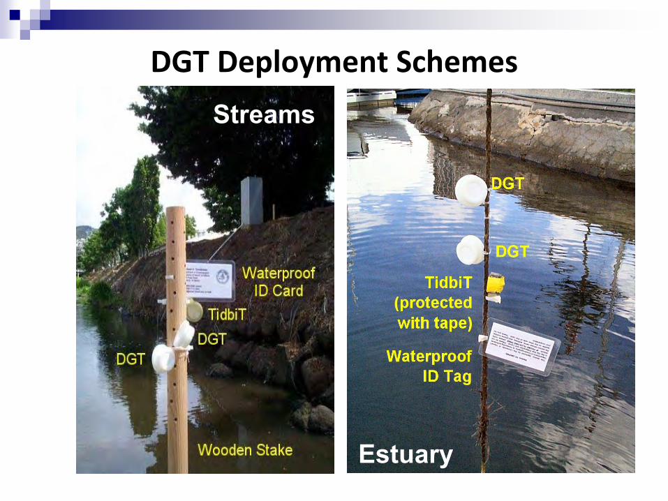
DGT Deployment Schemes
Estuary
Streams
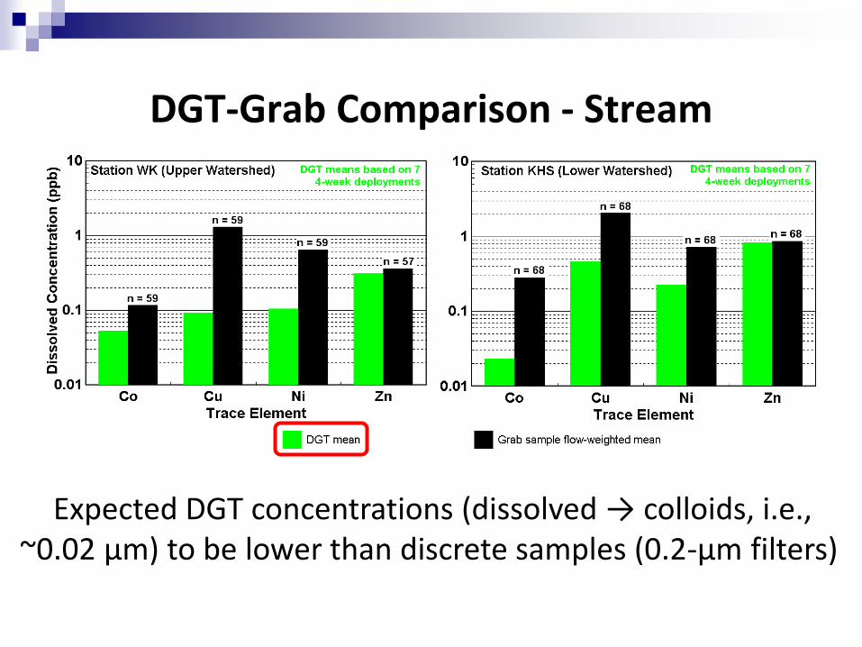
DGT-Grab Comparison - Stream
Expected DGT concentrations (dissolved → colloids, i.e., ~0.02 µm) to be lower than discrete samples (0.2-µm filters)
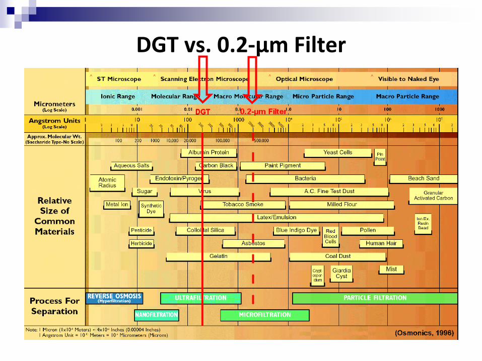
DGT vs. 0.2-µm Filter
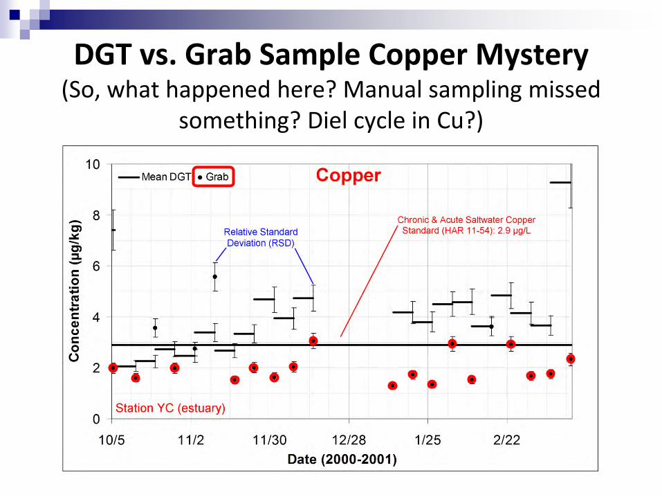
DGT vs. Grab Sample Copper Mystery (So, what happened here? Manual sampling missed
something? Diel cycle in Cu?)
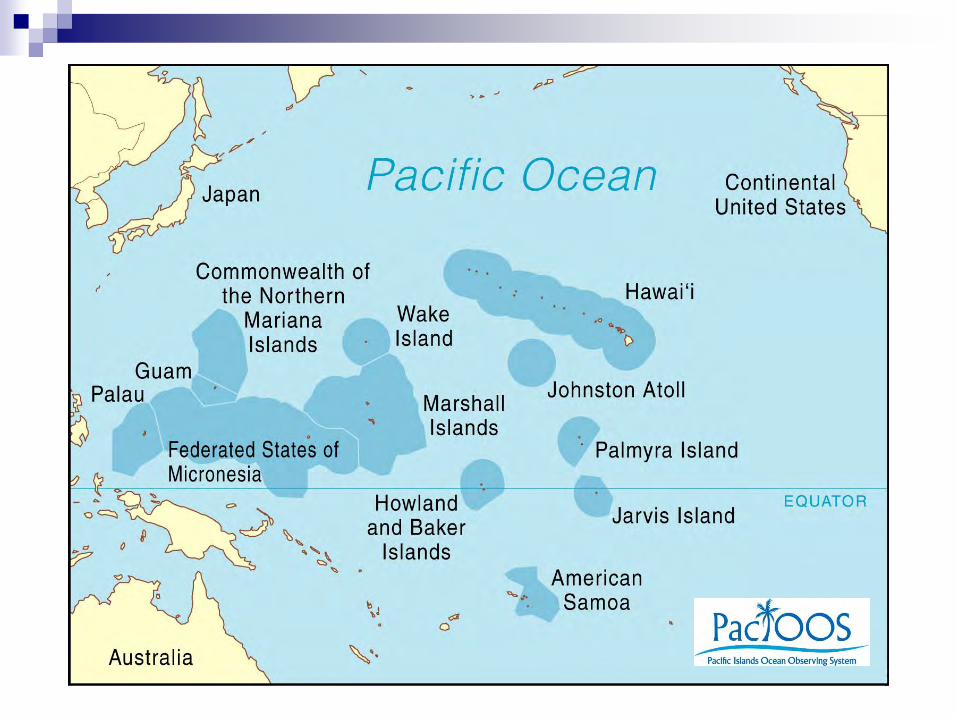
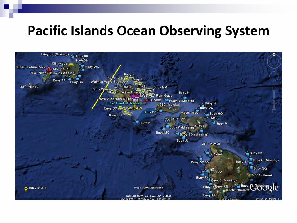
Pacific Islands Ocean Observing System
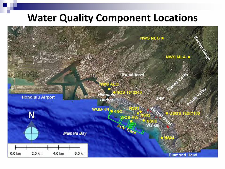
Water Quality Component Locations
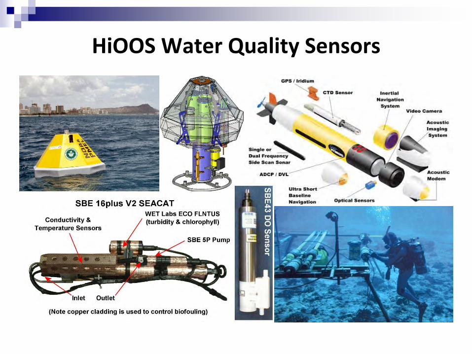
HiOOS Water Quality Sensors
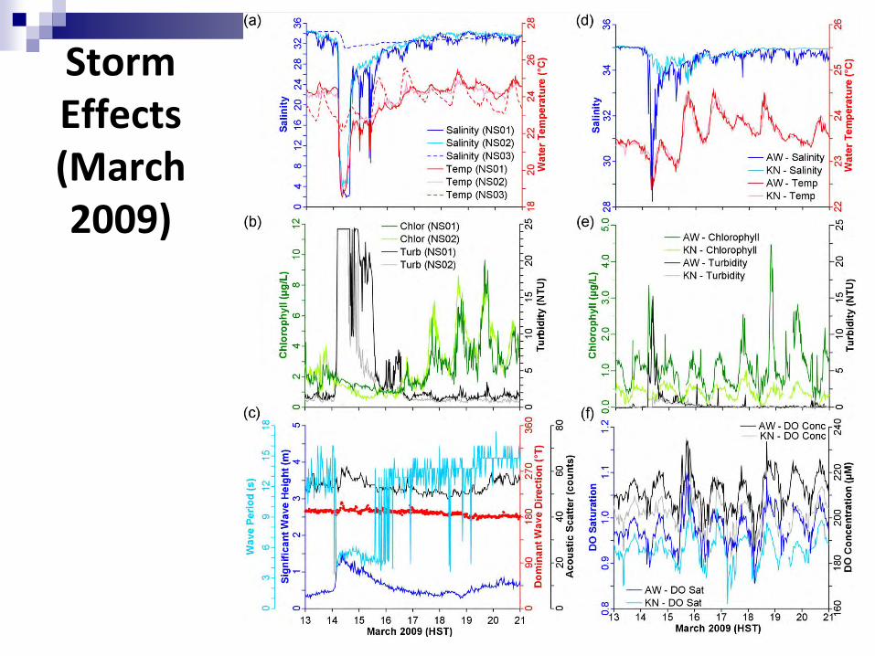
Storm Effects (March 2009)
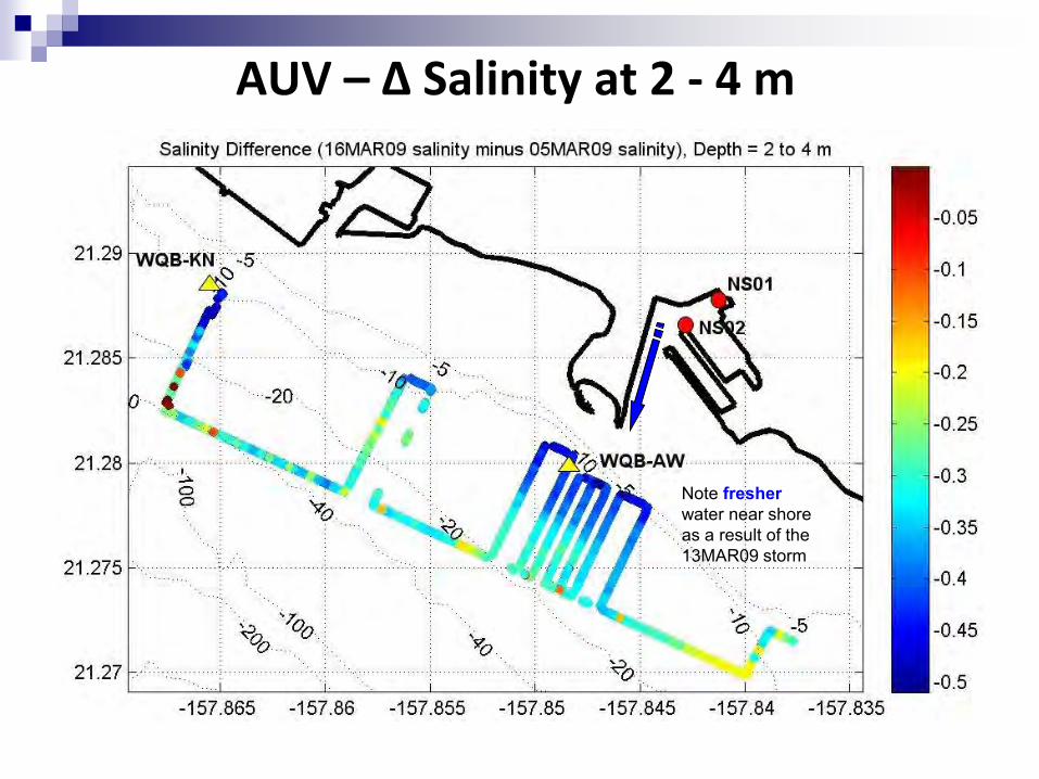
AUV – Δ Salinity at 2 - 4 m
Note fresher water near shore as a result of the 13MAR09 storm
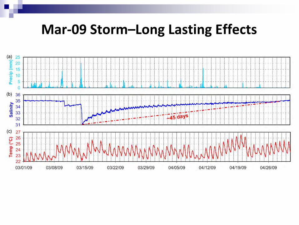
Mar-09 Storm–Long Lasting Effects
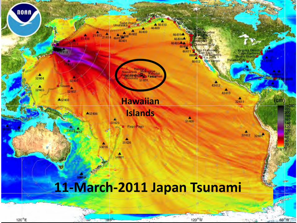
11-March-2011 Japan Tsunami
Hawaiian Islands
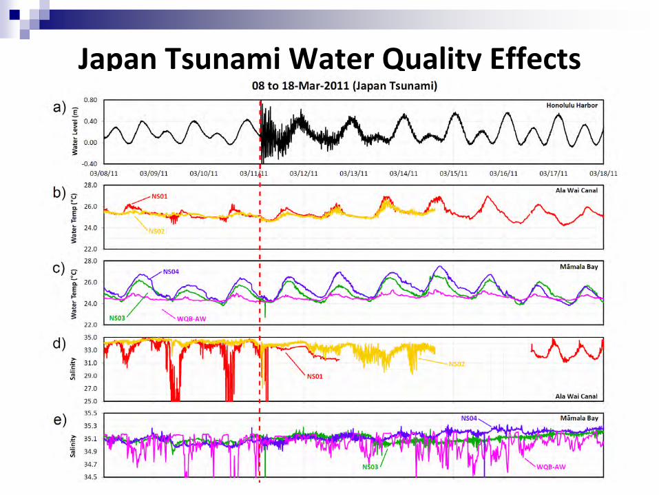
Japan Tsunami Water Quality Effects
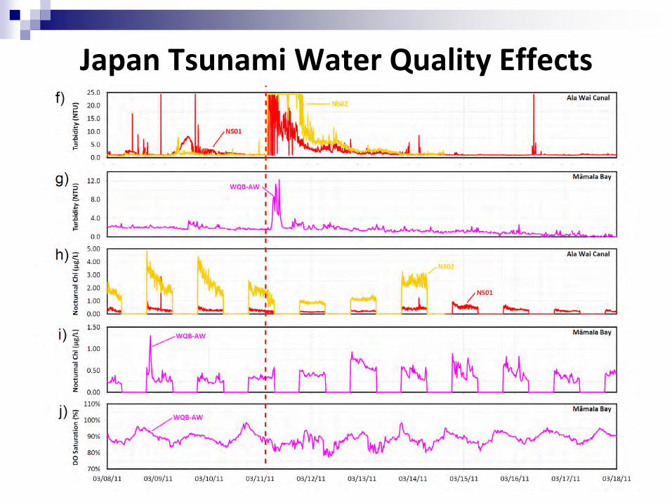
Japan Tsunami Water Quality Effects
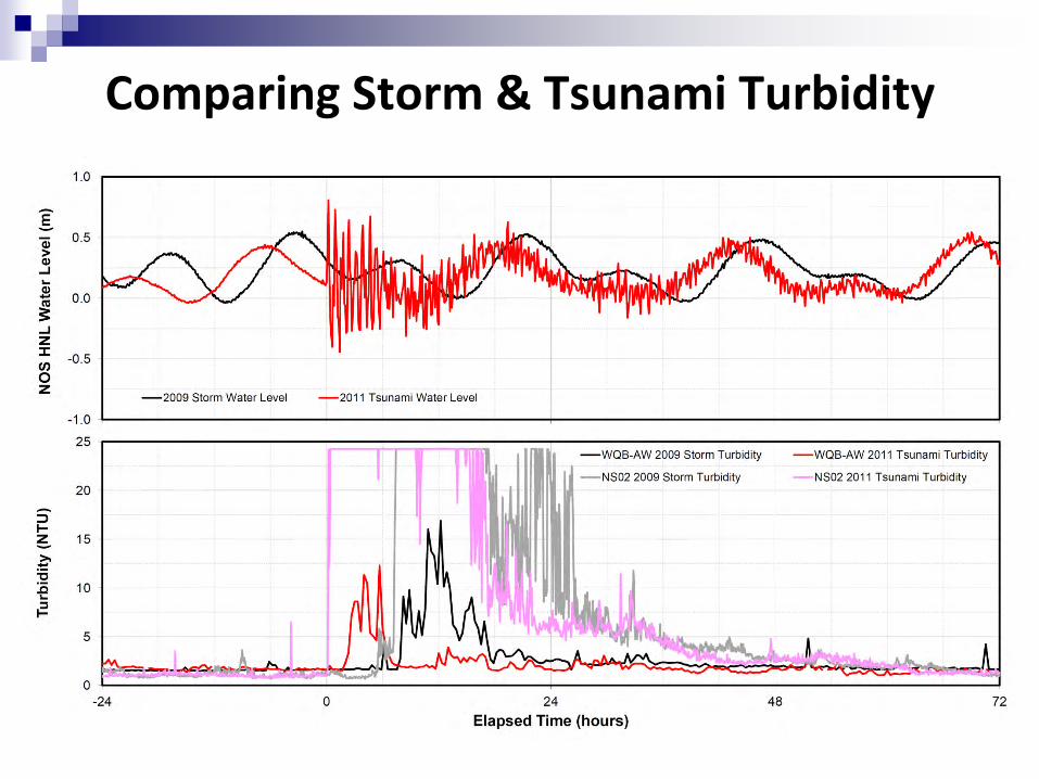
Comparing Storm & Tsunami Turbidity
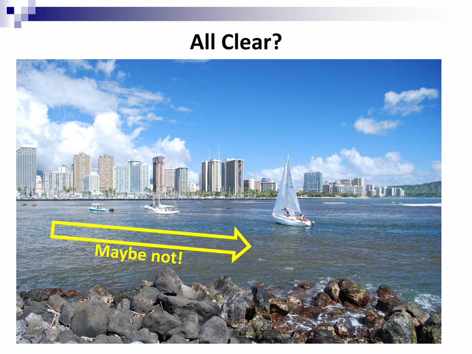
All Clear?
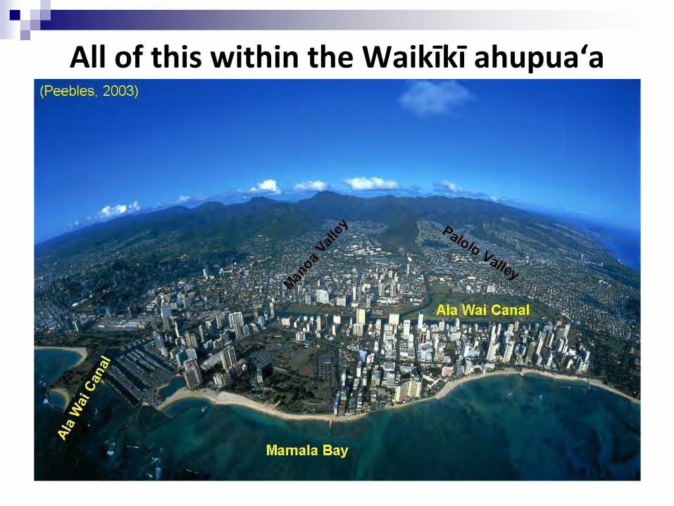
All of this within the Waikīkī ahupuaʻa
Mahalo! Questions?
Michael Tomlinson UHM Oceanography, Flagstaff, AZ 86004
928-266-2236, [email protected]

For attending the 2014 AIPG & AHS National Conference!
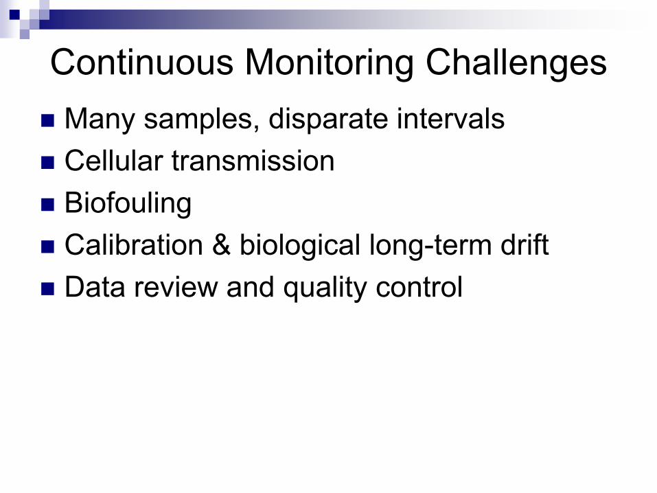
Continuous Monitoring Challenges Many samples, disparate intervals Cellular transmission Biofouling Calibration & biological long-term drift Data review and quality control
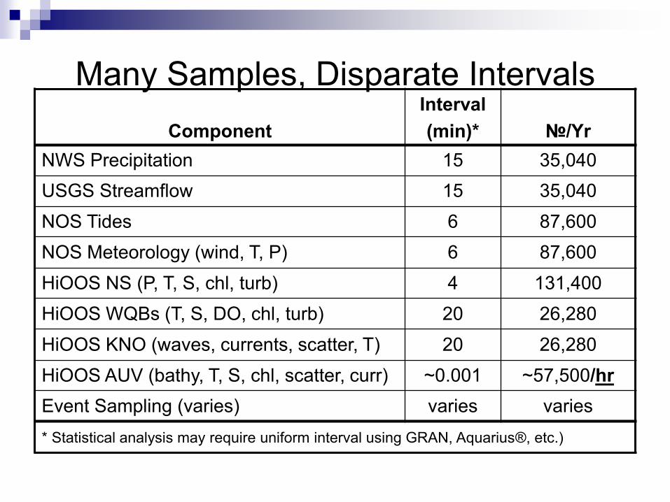
Many Samples, Disparate Intervals Component
Interval (min)* №/Yr
NWS Precipitation 15 35,040 USGS Streamflow 15 35,040 NOS Tides 6 87,600 NOS Meteorology (wind, T, P) 6 87,600 HiOOS NS (P, T, S, chl, turb) 4 131,400 HiOOS WQBs (T, S, DO, chl, turb) 20 26,280 HiOOS KNO (waves, currents, scatter, T) 20 26,280 HiOOS AUV (bathy, T, S, chl, scatter, curr) ~0.001 ~57,500/hr Event Sampling (varies) varies varies * Statistical analysis may require uniform interval using GRAN, Aquarius®, etc.)
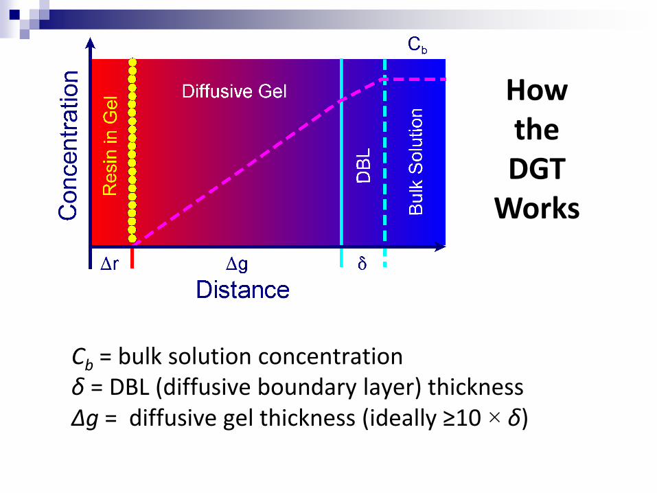
Cb = bulk solution concentration δ = DBL (diffusive boundary layer) thickness Δg = diffusive gel thickness (ideally ≥10 × δ)
How the DGT
Works
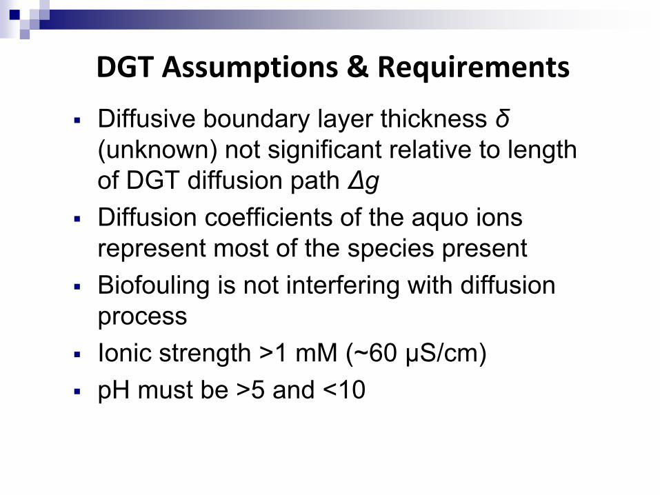
DGT Assumptions & Requirements
Diffusive boundary layer thickness δ (unknown) not significant relative to length of DGT diffusion path Δg
Diffusion coefficients of the aquo ions represent most of the species present
Biofouling is not interfering with diffusion process
Ionic strength >1 mM (~60 µS/cm) pH must be >5 and <10
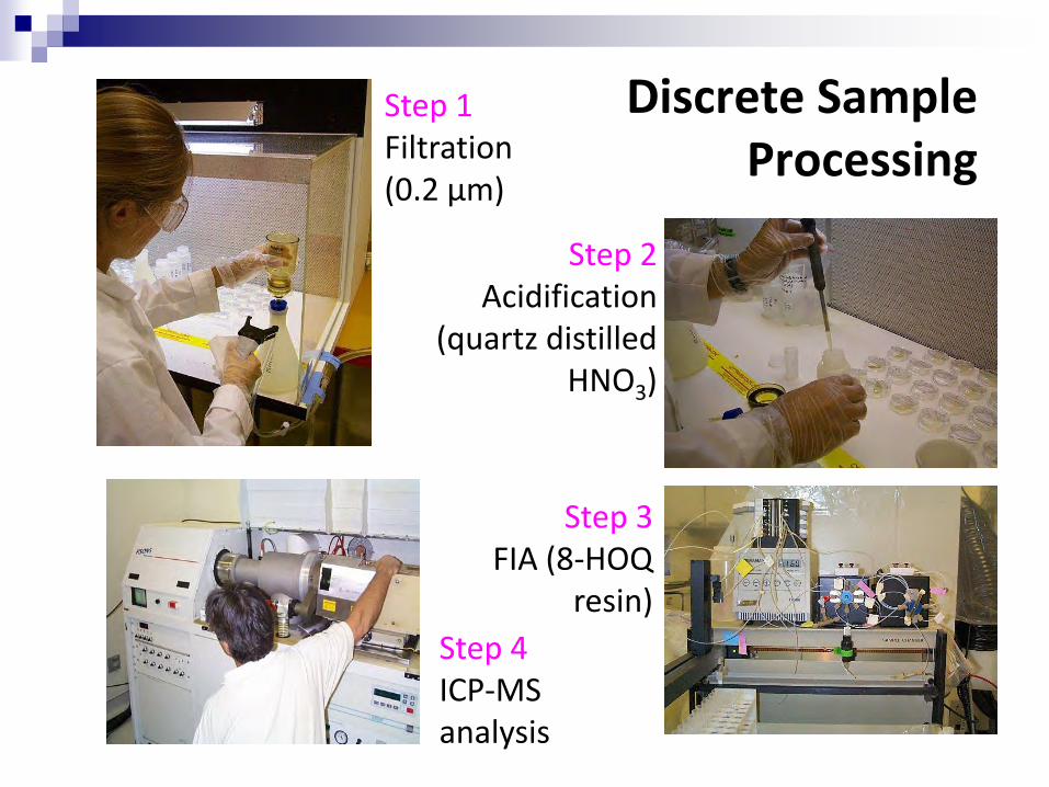
Discrete Sample Processing
Step 1 Filtration (0.2 µm)
Step 2 Acidification
(quartz distilled HNO3)
Step 3 FIA (8-HOQ
resin)
Step 4 ICP-MS analysis
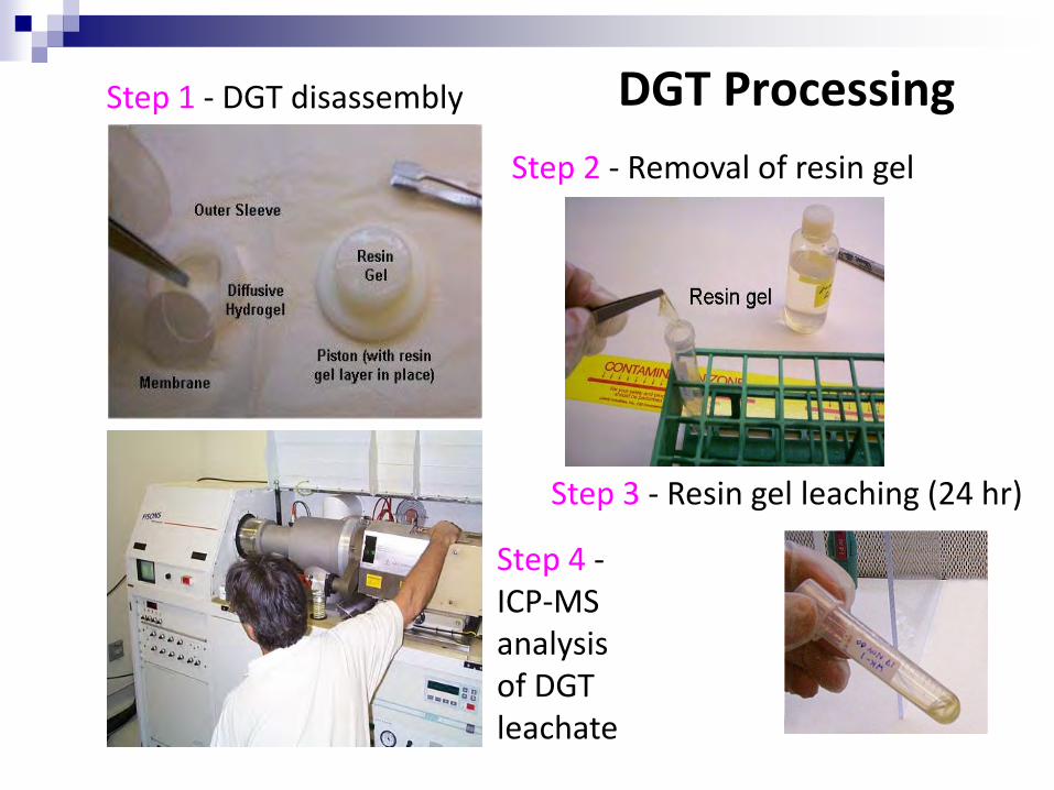
DGT Processing Step 1 - DGT disassembly
Step 2 - Removal of resin gel
Step 3 - Resin gel leaching (24 hr)
Step 4 - ICP-MS analysis of DGT leachate
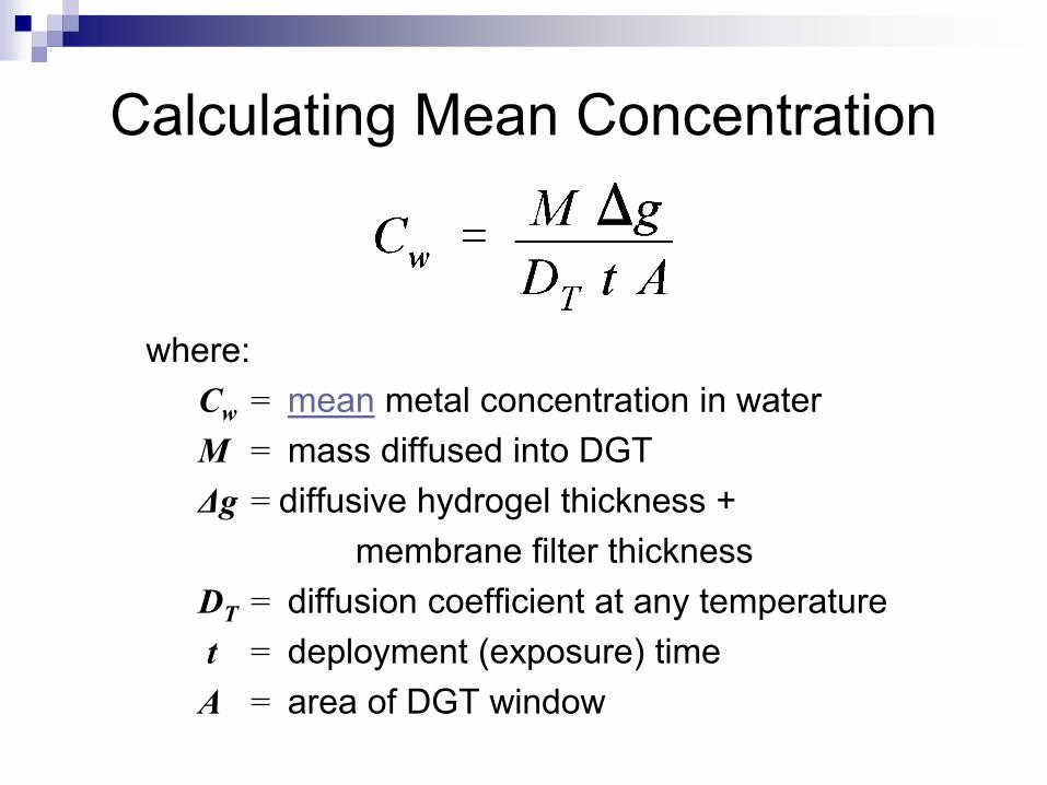
Calculating Mean Concentration
where: Cw = mean metal concentration in water M = mass diffused into DGT Δg = diffusive hydrogel thickness + membrane filter thickness DT = diffusion coefficient at any temperature t = deployment (exposure) time A = area of DGT window
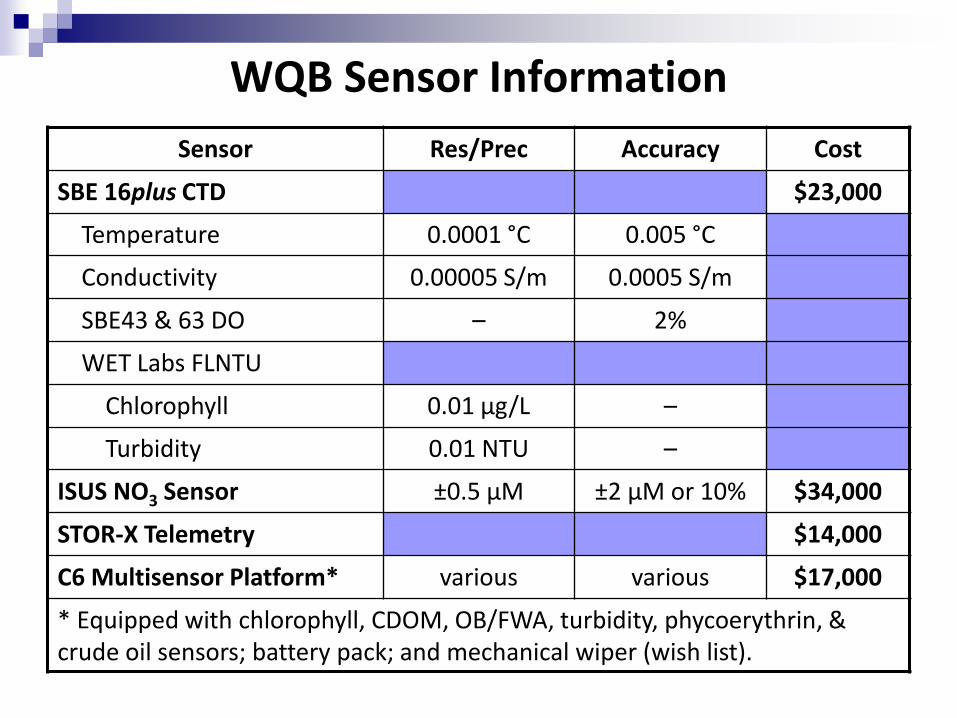
WQB Sensor Information
Sensor Res/Prec Accuracy Cost
SBE 16plus CTD $23,000
Temperature 0.0001 °C 0.005 °C
Conductivity 0.00005 S/m 0.0005 S/m
SBE43 & 63 DO – 2%
WET Labs FLNTU
Chlorophyll 0.01 µg/L –
Turbidity 0.01 NTU –
ISUS NO3 Sensor ±0.5 µM ±2 µM or 10% $34,000
STOR-X Telemetry $14,000
C6 Multisensor Platform* various various $17,000
* Equipped with chlorophyll, CDOM, OB/FWA, turbidity, phycoerythrin, & crude oil sensors; battery pack; and mechanical wiper (wish list).


![Kurzpräsentation über S-Monitoring Konzept und Produkte [DE]](https://img.dokumen.tips/doc/110x75/559ea42d1a28abff618b4789/kurzpraesentation-ueber-s-monitoring-konzept-und-produkte-de.jpg)