Embed Size (px)
Citation preview

Monitoring and Evaluating Nonpoint Source Watershed Projects Chapter 2
2-1
2 Nonpoint Source Monitoring Objectives and Basic Designs By S.A. Dressing, D.W. Meals, J.B. Harcum, and J. Spooner
Water quality monitoring is performed to support a wide range of programs. National-level monitoring with continuous water-quality monitors is performed by the USGS, for example, to assess the quality of the Nation’s surface waters (Wagner et al. 2006). Studies of large basins such as the Mississippi River Basin and Great Lakes Basin are designed to assess the general condition of waterbodies, track the health of fisheries, identify the causes and sources of designated beneficial use support impairments, and aid in the design of programs and projects to solve identified problems. EPA, states, and tribes conduct a series of surveys of the nation's aquatic resources that can also be used to track changes in condition over time. Each year the survey focuses on a different aquatic resource (i.e., rivers and streams, lakes, wetlands, or coastal waters) to yield unbiased estimates of the condition of the whole water resource being studied.1 Monitoring of smaller watersheds is done for a number of purposes, including assessing local water quality problems, developing watershed plans to address current and prevent future problems, and educating the public about the water environment. Monitoring of individual practices or BMPs is typically carried out to determine the effectiveness of the particular practices, provide data for the development or validation of watershed modeling tools, document efforts to address watershed-scale problems, and inform stakeholders.
2.1 Monitoring Objectives Monitoring is an information gathering exercise that is intended to generate data that serve management decision-making needs (USEPA 2003a). The formulation of clear monitoring objectives is an essential first step in developing an efficient and effective monitoring plan. Monitoring supports a range of water quality management objectives including establishing water quality standards, determining water quality status and trends, identifying impaired waters, identifying causes and sources of water quality problems, and evaluating program effectiveness. Specific objectives appropriate for NPS monitoring plans include:
Identify water quality problems, use impairments, causes, and pollutant sources.
Develop TMDLS and load or wasteload allocations.
Analyze trends.
Assess the effectiveness of BMPs or watershed projects.
Assess permit compliance.
Validate or calibrate models.
Conduct research.
1 http://water.epa.gov/type/watersheds/monitoring/aquaticsurvey_index.cfm
Monitoring and Evaluating Nonpoint Source Watershed Projects Chapter 2
2-2
Overview of Steps in Monitoring Design 1. Identify problem(s) 2. Form objectives 3. Design experiment 4. Select scale 5. Select variables 6. Choose sample type 7. Locate stations 8. Determine sampling frequency 9. Design stations 10. Define collection/analysis methods 11. Define land use monitoring 12. Design data management
(USDA-NRCS 2003)
All monitoring programs should be designed to answer questions. The design process begins with identifying the problem and setting objectives that pose the questions. Then an experimental design appropriate to those objectives is selected and decisions related to sample type, sampling locations, which variables to monitor, and how to collect and analyze the samples that need to be made. Because the purpose of NPS monitoring is often to evaluate practice effectiveness and programs taking place on the land, land use and land management monitoring is an integral part of the overall effort. Finally, management and analysis of data gathered through the monitoring program must also be incorporated.
The specific steps essential in designing a monitoring program to meet objectives are discussed in detail in this chapter and chapter 3.
EPA and states need comprehensive water quality monitoring and assessment information to help set levels of protection in water quality standards. This information will also help to identify emerging problem areas or areas that need additional regulatory and non-regulatory actions to support water quality management decisions such as TMDLs, NPDES permit limits, enforcement, and NPS management (USEPA 2003a). Statewide monitoring to assess the degree to which designated beneficial uses (e.g., drinking, swimming, aquatic life) are supported is an essential component of efforts to achieve CWA goals. For example, CWA §106(e)(1) and 40 CFR Part 35.168(a) provide that EPA award Section 106 funds to a state only if the state has provided for or is carrying out the establishment and operation of appropriate devices, methods, systems and procedures necessary to monitor and to compile and analyze data on the quality of its navigable waters. States must also update the data in the Section 305(b) report.
In accordance with EPA water quality standards regulations, states designate uses for each waterbody or waterbody segment and establish criteria (e.g., dissolved oxygen [DO] levels, temperature, metals concentrations) that must be met through their water quality standards programs. Monitoring of the criteria parameters is then performed to assess whether the criteria are being met (USEPA 2003b). Biological monitoring of aquatic systems has been increasingly used to assess aquatic life use support.
Because of the magnitude of the task, states generally monitor portions of the state on a rotating basis (USEPA 2011). Ohio, for example, has a 15-year plan for monitoring all 8-digit HUCs in the state (OEPA 2013). Each year Ohio EPA collects data from streams and rivers in five to seven different areas of the state. A total of 400 to 450 sampling sites are examined, and each site is visited more than once per year. During these studies, Ohio EPA technicians collect chemical samples, examine and count fish and aquatic insects, and take measurements of the stream. There are three major objectives for the studies:
Determine how the stream is doing compared to goals assigned in the Ohio Water Quality Standards;
Determine if the goals assigned to the river or stream are appropriate and attainable; and
Determine if the stream’s condition has changed since the last time the stream was monitored.

Monitoring and Evaluating Nonpoint Source Watershed Projects Chapter 2
2-3
The findings of each biological and water quality study can be used in Ohio EPA regulatory actions. The results are incorporated into Water Quality Permit Support Documents, State Water Quality Management Plans, and the Ohio Nonpoint Source Assessment. This information also provides the basis for the Integrated Water Quality Monitoring and Assessment Report – a biennial statewide report on the condition of Ohio’s waters and the list of impaired and threatened waters required by sections 303(d) and 305(b) of the Clean Water Act.
The growing linkage between the national NPS and TMDL programs has resulted in a greater emphasis on estimating pollutant loads (USEPA 2003b). Specific considerations and recommendations for monitoring to estimate pollutant loads are presented in section 3.8. Development of load-duration curves has become an important step in developing TMDLs for many watersheds, and this topic is addressed in detail in section 8.9.4.
Well-formulated monitoring objectives drive the rest of the monitoring study design and are critical to a successful monitoring project (USDA-NRCS 2003). It is also important that monitoring objectives are directly linked to overall program or project objectives that depend on the monitoring data. Table 2-1 illustrates this important linkage between program and monitoring objectives.
Table 2-1. Complementary program and monitoring objectives Program Objective Complementary Monitoring Objective Reduce annual P loading to lake by at least 15 percent in 5 years with nutrient management
Measure changes in annual P loading to lake and link to management actions
Reduce E. coli load to stream to meet water quality standards in 3 years
Measure changes in compliance with water quality standard for E. coli
A good example to illustrate the development of program goals, supporting monitoring goals, and specific monitoring designs is the USGS National Water-Quality Assessment Program (NAWQA). NAWQA was designed to assess the status and trends in the nation's ground- and surface-water resources and to link the status and trends with an understanding of the natural and human factors that affect water quality (Gilliom et al., 1995). The study design balanced the unique assessment requirements of individual hydrologic systems with a nationally consistent design structure that incorporated a multi-scale, interdisciplinary approach. The Occurrence and Distribution Assessment, the most important component of the first intensive study phase in each of the NAWQA study units, was intended to characterize, in a nationally consistent manner, the broad-scale geographic and seasonal distributions of water-quality conditions in relation to major contaminant sources and background conditions. General goals for study-units were:
Identify the occurrence of water quality conditions that are significant issues.
Characterize the broad-scale geographic and seasonal distribution of a wide range of water quality conditions in relation to natural factors and human activities.
Evaluate study-unit priorities and required study approaches for effectively assessing long-term trends and changes.
Evaluate geographical and seasonal distribution in greater detail and in relation to the sources, transport, fate and effects of contaminants for water quality conditions of greatest importance. Determine the priorities and design for follow-up case studies.

Monitoring and Evaluating Nonpoint Source Watershed Projects Chapter 2
2-4
USGS developed a study design to address each of the above goals for stream monitoring, employing three interrelated components: water-column, bed sediment and tissue, and ecological studies. Ecological studies incorporate three strategies:
Fixed-Site Reach Assessments provide nationally consistent ecological information at water column sites as part of an integrated physical, chemical, and biological assessment of water quality.
Intensive Ecological Assessments assess spatial and temporal variability associated with biological communities and habitat characteristics.
Ecological Synoptic Studies provide improved spatial resolution of selected ecological characteristics in relation to land uses, contaminant sources, and habitat conditions.
While the NAWQA program is an exceptionally large monitoring program in both scope and scale, the approach of linking monitoring to program goals and developing clear and specific monitoring goals and objectives to drive monitoring program design is applicable to most if not all monitoring efforts.
2.2 Fundamentals of Good Monitoring Water quality monitoring is a complex and demanding enterprise. Conducted well, monitoring can provide fundamental information about the water resource and its impairments. Monitoring data can allow managers to document changes through time, show response to NPS pollution reduction practices and programs, and confirm achievement of management objectives. Conducted poorly, monitoring can fail to meet objectives, create confusion, leave critical questions unanswered and waste time and money. It is essential that monitoring be designed to meet project and program objectives efficiently. The purpose of this section is to present key elements of good monitoring design and execution.
2.2.1 Understand the System When little is known about a watershed, monitoring may be used to assess the problem. For this purpose, monitoring requires a fairly general approach, e.g., reconnaissance or synoptic sampling (see section 2.4.2.1). When designing a monitoring program to assess a response to nonpoint source control programs, a thorough understanding of the system (e.g., a farm, an urban catchment, or a rural watershed) is required. An early step in watershed planning and management is characterization of the watershed, which includes topography, geology, climate, soils, hydrology, biota, land use, infrastructure, and cultural resources (USEPA 2008b). This is essential information about the system and will assist in the design of the monitoring system. The first of EPA’s Nine Key Elements of watershed restoration plans requires identification of the causes of impairment and the sources of pollutants that will need to be controlled to achieve the goals of the watershed plan (USEPA 2008b). Basic questions that should be addressed when characterizing a watershed include:
What are the critical water quality impairments or threats?
What are the key pollutants involved?
What are the sources of these pollutants?
How are pollutants transported through the watershed?
What are the most important drivers of pollutant generation and delivery?

Monitoring and Evaluating Nonpoint Source Watershed Projects Chapter 2
2-5
2.2.1.1 Causes and Sources Decisions on where, when, and how often to sample, what to measure, and other elements of monitoring design depend on knowledge of the watershed being monitored. The source of pollutants is an obvious issue. For example, suspended sediment exported from a watershed may arise from upland erosion from agricultural fields, streambank and streambed erosion, or a combination of both. Knowledge of the source of suspended sediment measured at the watershed outlet is essential to designing a system to monitor watershed response to implementation of erosion control measures (as well as in selection of the appropriate control measures). In Minnesota, for example, Sekely et al. (2002) estimated that streambank sources accounted for 31 percent to 44 percent of the suspended sediment load at the mouth of the Blue Earth River. Allmendinger et al. (2007) reported that upland sediment production and sediment from enlargement of stream channels were approximately equal sources of sediment yield in an urbanizing watershed in Maryland. Unusually high mean NO3-N concentrations (about 5 mg/l in the major tributaries) in watersheds that drain into the western and central basins of Lake Erie are thought to reflect the extensive use of tile drainage systems in the region (Baker 1988).
Indicator bacteria like fecal coliform or E. coli commonly cause impairment of recreation and shellfish harvesting in U.S. waters. These organisms can arise from numerous sources in a watershed, including wildlife, livestock, pets, and human wastes. It is essential to know the source(s) of these organisms both to apply the right control measures and to monitor response to control programs. For example, in the Oak Creek Canyon (AZ) NNPSMP project seasonal increases in fecal indicator bacteria were initially believed to originate primarily from poor sanitation practices by recreational users and a lack of adequate restroom facilities (Donald et al. 1998). Bacteriological water quality failed to improve after sanitation BMPs were installed, however, and analysis of fecal coliform levels in sediments versus those in the water column led to the conclusion that resuspension of contaminated sediments by recreational users and major storm events was the major cause of water quality violations. While sediment was identified as the major reservoir of bacteria, this analysis fell short of identifying the primary source(s) of the bacteria found in the sediment. DNA fingerprinting was used to determine the relative contributions of human, livestock, and wildlife sources, resulting in the finding that wildlife contributed a greater share of fecal pollution than humans. Still, at the conclusion of the NNPSMP project questions remained regarding the major sources of fecal contamination in the watershed (Donald et al. 1998, Spooner et al. 2011). A subsequent study by Poff and Tecle (2002) suggested that domesticated and wild animals, residential homes (septic systems), and business establishments were probably greater sources of E. coli than recreational visitors. Monitoring and BMP implementation have continued in the Oak Creek watershed, with establishment of a TMDL for E. coli in 2010 and completion of a watershed implementation plan in 2012 (OCWC 2012). Implementation efforts are now focused on education and outreach as the top priority, followed by septic systems, stormwater, recreation, and agriculture (OCWC 2012). Continued uncertainty regarding sources of fecal pollution is reflected by plan recommendations for additional monitoring of Oak Creek sediment to identify E. coli sediment reservoir hot spots and locate up-gradient sources of E. coli.
2.2.1.2 Pollutant Transport It is absolutely critical to understand the mode of pollutant transport through the watershed from source to receiving water before setting up a monitoring system. Particulate pollutants, such as sediment and attached substances, generally move in surface waters. Monitoring for sediment or particulate phosphorus is generally best focused on surface runoff and streamflow. Dissolved pollutants, like nitrate-nitrogen (NO3-N), are transported in both surface and ground waters. The relative importance of these distinct pathways needs to be understood to decide where and when to sample. For example in the Chesapeake Bay watershed, it is estimated that 40 percent of the annual N load to the Bay is delivered by groundwater

Monitoring and Evaluating Nonpoint Source Watershed Projects Chapter 2
2-6
(STAC 2005). As much as 80 percent of annual export of NO3-N, sulfate (SO -24 ), and chloride (Cl-1) from
small Iowa watersheds occurred in baseflow (Schilling 2002).
In many cases, additional details regarding pollutant pathways must be understood to fine tune monitoring plans. For example, decisions on whether to focus on high-flow events (e.g., for particulate pollutants delivered episodically in surface runoff or storm flows) or base flows (e.g., for dissolved pollutants that tend to be delivered continuously via ground water) require an understanding of how pollutants move through the system. The Warner Creek (MD) NNPSMP discovered that base flow contributed 76 percent of total streamflow and that subsurface flow, including a substantial portion from outside the surface watershed boundaries, was the major pathway for transport of NO3-N to the stream (Shirmohammadi et al. 1997, Shirmohammadi and Montas 2004). This complex hydrology contributed to the failure of an above/below monitoring design for this project.
The timing of sampling during storm events can also be informed by knowledge of pollutant pathways. For example, analysis of long-term data collected in the Lake Erie basin showed that peak concentrations of particulate and soluble pollutants occurred during different parts of the storm hydrograph (Baker et al. 1985, Baker 1988). TP and sediment concentrations reached their peak early in the runoff event before peak discharge, and decreased faster than the discharge decreased. The TP concentration did not decline as rapidly as the sediment concentration due to the presence of soluble P and an increasing ratio of particulate P to sediment as the sediment concentration decreased. The atrazine concentration pattern followed the hydrograph very closely, indicating movement off the fields with surface runoff water. Nitrate (NO3) increased during the falling limb of the hydrograph due to tile drainage and interflow.
2.2.1.3 Seasonality Seasonal patterns are often critical factors in monitoring design because NPS pollution is highly weather-driven. In northern regions, snowmelt and spring rains are often the dominant hydrologic feature of the annual cycle and a majority of the annual pollutant load may be delivered in a few weeks. A seven-year study on corn-cropped watersheds in southwestern Iowa, for example, showed that most of the average annual total N and P losses occurred during the fertilizer application, seedbed preparation, and crop establishment period from April through June (Alberts et al. 1978). February accounted for 23 percent of the total P load in a two-year study in the Clear Lake watershed in Iowa, indicating that the snowmelt period is a time of significant P loss from fields (Klatt et al. 2003). In Wisconsin, Stuntebeck et al. (2008) stated that it was critical that agricultural NPS monitoring take place year-round to fully characterize sediment and nutrient losses throughout the year rather than just during the growing season.
For herbicides such as atrazine, losses from agricultural fields in humid areas are highly episodic, with the majority of annual losses occurring in transient storm events soon after herbicide application. In a comparative study of agricultural watersheds in different climatic regions, Domagalski et al. (2007) found that stormwater runoff after application was the primary determinant of pesticide loads in humid environments. A significant portion of the load of some pesticide degradation products, however, can be transported under base-flow conditions in humid environments. In such cases, a monitoring effort would need to reliably monitor short, intense and unpredictable events during specific seasons, depending on both seasonal and agronomic factors. Sampling of base flow would be needed to track degradation products. The same comparative study, however, found that irrigation practices and timing of chemical use greatly affected pesticide transport in the semiarid basins, suggesting a monitoring effort that would need to be focused on irrigation events in these regions.

Monitoring and Evaluating Nonpoint Source Watershed Projects Chapter 2
2-7
The importance of characterizing seasonality depends on the specific program and monitoring objectives. In cases where available water quality data are not sufficient to assess seasonality in a specific watershed, it may be necessary to perform seasonal synoptic surveys (see section 2.4.2.1), collect year-round samples initially, or rely on watershed modeling to better define seasonality and facilitate fine-tuning of the monitoring design.
2.2.1.4 Water Resource Considerations Each type of water resource—rivers and streams; lakes, reservoirs, and ponds; wetlands; estuaries; coastal shoreline waters; and ground water—possesses unique hydrologic and biological features that must be considered in the design of a monitoring program. All water resource types exhibit both temporal (long- and short-term) and spatial (small- and large-scale) variability. For example, suspended sediment concentrations vary with depth and location in reservoirs; salinity concentrations in estuaries vary vertically and horizontally, as well as temporally as they are affected by relatively light fresh water flowing over heavier salt water; and ground water quality varies with soil and aquifer type and geozone. Placement of monitoring stations and the timing and duration of sampling are affected by consideration of these and other sources of variability.
2.2.1.4.1 Rivers and Streams Streams can be classified at various levels of detail using a number of criteria (e.g., Montgomery and Buffington 1997, Rosgen and Silvey 1996), but streams can also be lumped for monitoring considerations into two major groups – intermittent and perennial – based simply on general flow characteristics. Clearly, water quality sampling cannot be conducted in intermittent streams when they do not have flow; however, the ability to measure and sample intermittent flows when they do occur is often critical and usually challenging. Year-to-year variations in precipitation can have major impacts on flow duration and frequency, pollutant loads, and water quality in intermittent streams. Flow in perennial streams and rivers is also affected by seasonal rainfall and snowfall patterns, reservoir discharge management, and irrigation management. Pollutant loads and concentrations, in turn, are affected by these patterns as the highest concentrations of suspended sediment and nutrients often occur during spring runoff, winter thaws, or intense rainstorms.
Because good flow measurement is essential to estimating pollutant loads, it is also important to understand spatial flow patterns in the monitored stream or river. Water velocities vary both horizontally (e.g., outside vs. inside meander bends) and vertically with depth (USDA-NRCS 2003, Meals and Dressing 2008). In addition, the complexity of currents at obstructions and points of constriction (e.g., bridges) makes them poor monitoring sites (Meals and Dressing 2008). Rudimentary stream classification can be very helpful in predicting a river's behavior from its appearance, which, in turn, can be useful in identifying locations for fixed sampling stations. Flow measurement is discussed in greater detail in section 3.1.3.1.
Flow patterns often play a significant role in determining the variability of water quality, both within a stream cross-section and throughout a stream reach. Figure 2-1 illustrates the relationship between pollutant concentrations and the vertical variability of stream velocity (Brakensiek et al. 1979). The effects of tributary flows must be considered when designing a stream or river monitoring program. Such flows can add pollutant loads, dilute pollutant loads, and create horizontal gradients. In some cases mixing below tributary junctions might be incomplete, with tributary flow primarily following one bank or forming spatially and temporally persistent plumes or bands (Sommer et al. 2008). If a representative sample of a river is required, it is important to select a sampling point where the flow is uniform and well-mixed, without sharp flow variations or distinct tributary inflow plumes. If more detail is required,

Monitoring and Evaluating Nonpoint Source Watershed Projects Chapter 2
2-8
segmentation of a stream into fairly homogeneous segments prior to monitoring might be necessary, with one to several monitoring stations located in each segment (Coffey et al. 1993). When dividing a stream into homogeneous segments, both land use and drainage area should be considered because both affect the quantity and quality of flows.
Figure 2-1. Vertical sediment concentration and flow velocity distribution in a typical stream cross section (after Brakensiek et al. 1979)
Vertical variability is particularly important during runoff events and in slow-moving streams because suspended solids, dissolved oxygen (DO), and algal productivity can vary substantially with depth (Figure 2-2) (Brakensiek et al. 1979). Levels of contaminants in bed sediment also vary horizontally and vertically, as deposition and scouring are strongly influenced by water velocity.
Biological communities in stream systems vary with a number of factors including landscape position, type of substrate, light, water temperature, current velocity, and amount and type of aquatic and riparian vegetation. Monitoring of aquatic communities is discussed in chapter 4.

Monitoring and Evaluating Nonpoint Source Watershed Projects Chapter 2
2-9
Figure 2-2. Schematic diagram of stream vertical showing position of sediment load terms (after Brakensiek et al. 1979)
2.2.1.4.2 Lakes, Reservoirs, and Ponds Lakes are defined here as natural standing or slow-moving bodies of water. Reservoirs are considered to be human-made lakes typically created by impounding a river or stream. Ponds can be either natural or human-made, and are generally much smaller and shallower than lakes. The following discussion focuses primarily on lakes and reservoirs with lake referring to both types of water bodies.
Lakes are more than simple bowls of water. The physical, chemical, and biological characteristics of lakes vary horizontally, vertically, seasonally, and throughout the day. In addition, reservoirs can exhibit characteristics of both rivers and lakes, with the upstream section more river-like and downstream areas near the dam more lake-like. The balance between river and lake characteristics can vary widely among reservoirs with some more river-lake throughout. This variability must be understood and considered when designing a lake monitoring program.
Hydrology and geomorphology are strong determinants of the physical, chemical, and biological characteristics of lakes (Wetzel 1975). Lakes can be classified based on how water enters and exits the lake: seepage lakes, spring lakes, groundwater drained lakes, drainage lakes, and impoundments (WAL 2009). Knowledge of the primary sources of water and the presence or absence of inlets and outlets is essential to determining options for an effective monitoring plan.
Lake shape has major implications for monitoring design. Lakes and ponds with simple, rounded shapes may tend to be well-mixed at most times and might require only a single sampling station to provide an accurate representation of water quality. Lakes with complex interconnected basins or with dendritic shapes like reservoirs tend to exhibit significant spatial variability as mixing is inhibited; such lakes may require numerous sampling stations to represent more uneven water quality characteristics (USEPA
Monitoring and Evaluating Nonpoint Source Watershed Projects Chapter 2
2-10
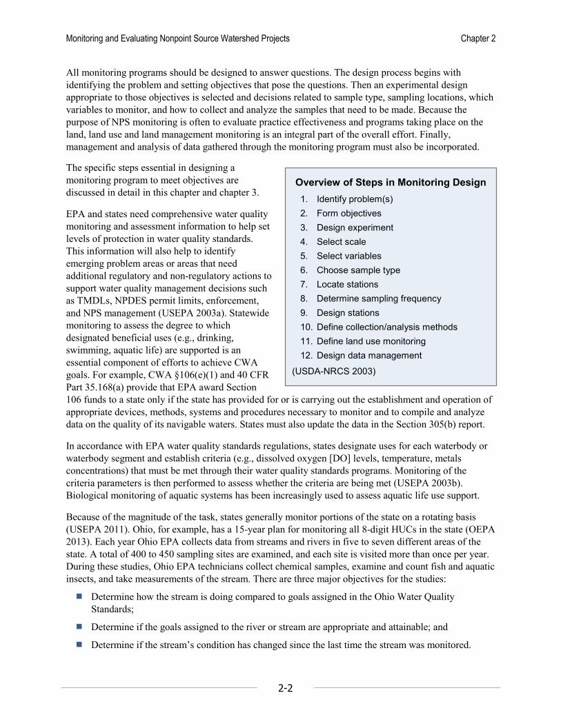
1990). In Lake Champlain (VT-NY-Quebec) for example, the lake’s complex geometry of bays, islands, and bathymetry generally divide the lake into five distinct regions for monitoring (Figure 2-3).
Figure 2-3. Map of water quality monitoring stations in Lake Champlain lake regions (Lake Champlain Basin Program)

Monitoring and Evaluating Nonpoint Source Watershed Projects Chapter 2
2-11
Tributary inflows and effluent discharge points also contribute to horizontal variations in lake water quality. Localized inputs of large water and/or pollutant loads – e.g., suspended sediment from a large tributary river basin draining agricultural land or a nutrient load from a WWTP – can influence localized water quality, especially in a confined bay. Locations of such discharges are key factors in placing monitoring stations – either to deliberately sample them to represent important localized impairments or distinct components of total lake inputs, or to deliberately avoid them as unrepresentative of the broad lake, depending on program objectives.
Vertical variability in lakes can affect water quality and consequently monitoring design choices. Uniformly shallow lakes such as Grand Lake St. Marys in Ohio (GLWWA 2009) tend to be well-mixed vertically and have extensive photic zones, yielding a fairly homogeneous water column that can be effectively sampled at a single depth. Deeper lakes tend to stratify seasonally because of the temperature-density properties of water (Figure 2-4). Vertical stratification in lakes and reservoirs depends largely on depth, temperature, and seasonality, all of which should be included as covariates when monitoring lakes. When stratification is strong, the upper waters (epilimnion) may exhibit water quality characteristics (e.g., warm temperatures, high DO, low dissolved P) very different from those of the lower waters (hypolimnion) (e.g., cold temperatures, low DO, high dissolved P) because the two layers do not mix readily for long periods of time. This stratification breaks down in many lakes during fall and spring, when the water column mixes due to wind (turnover) and water quality is more uniform vertically. Depending on study objectives (e.g., monitoring algae populations in the epilimnion or measuring oxygen depletion in the hypolimnion), monitoring at different points with depth during periods of peak stratification may be appropriate. Alternatively, sampling during the periods when the water column is completely mixed (e.g., at spring or fall turnover) may yield information on the general character of the lake for that year. Some mass-balance lake P models, for example, use P concentration at spring turnover to represent the overall nutrient status of the lake.
Vertical variability is also important in lake biological monitoring. Chlorophyll levels and phytoplankton populations are naturally concentrated in the upper waters where sunlight can penetrate (the photic zone). However, zooplankton are mobile and show diurnal vertical migrations, moving up in the water column at night to feed and down during the day to avoid predators (Lampert 1989, Stich and Lampert 1981, Zaret and Suffern 1976).
Lake currents (primarily wind and inflow-driven) influence the dispersal of pollutants in a lake. In a reservoir, pollutant concentrations may exhibit a longitudinal gradient as circulation is dominated by inflow from the main tributary and outflow at the dam. Conditions in small embayments can be very different from conditions in open water. These conditions are due to circulation patterns caused by prevailing winds if currents tend to retain pollutants in the bay and inhibit mixing with the main lake waters.
Finally, sediment/water interactions exert strong controls on some pollutant dynamics in lakes. Concentrations of pollutants like P or toxic compounds that are strongly adsorbed to sediment particles can vary across the lakebed as sediments delivered from large tributary river basins settle around tributary mouths or are moved by currents into deeper lake regions. These dynamics may lead to hot-spots of high sediment pollutant levels that could be important for biological monitoring. In some cases, bottom sediments store pollutants like P for long periods as particles settle out over time or even sorb P from the water. In other cases, (especially where bottom waters are low in oxygen), P and other pollutants can be released from lake sediments to add to the lake pollutant load. Consequently, sediment remediation is sometimes part of efforts to reduce in-lake P concentrations, e.g., dredging (GLWWA 2009) or alum treatment (Welch and Cook 1999).

Monitoring and Evaluating Nonpoint Source Watershed Projects Chapter 2
2-12
Figure 2-4. Thermally stratified lake in mid-summer (USEPA 1990). Curved solid line is water temperature. Open circles are DO in an unproductive (oligotrophic) lake and solid circles are DO in a productive (eutrophic) lake.
2.2.1.4.3 Wetlands Since 1979, the Fish and Wildlife Service’s definition of a “wetland” has been accepted as a standard for purposes of collecting information on the location, characteristics, extent, and condition of wetlands (Tiner 2002):
Wetlands are lands transitional between terrestrial and aquatic systems where the water table is usually at or near the surface or the land is covered by shallow water. For purposes of this classification wetlands must have one or more of the following three attributes: 1) at least periodically, the land supports predominantly hydrophytes (plants adapted to grow in water or hydric soils); 2) the substrate is predominantly undrained hydric soil (waterlogged or flooded soils); and 3) the substrate is nonsoil and is saturated with water or covered by shallow water at some time during the growing season of each year.”
Monitoring and Evaluating Nonpoint Source Watershed Projects Chapter 2
2-13
Three factors (hydrology, the presence of hydric soils, and the presence of hydrophytic vegetation) largely determine the characteristics of wetlands, but hydrology is considered the master variable of wetland ecosystems, driving the development of wetland soils and leading to the development of the biotic communities (USEPA 2004). All three factors, however, serve as the foundation of any wetland condition assessment method.
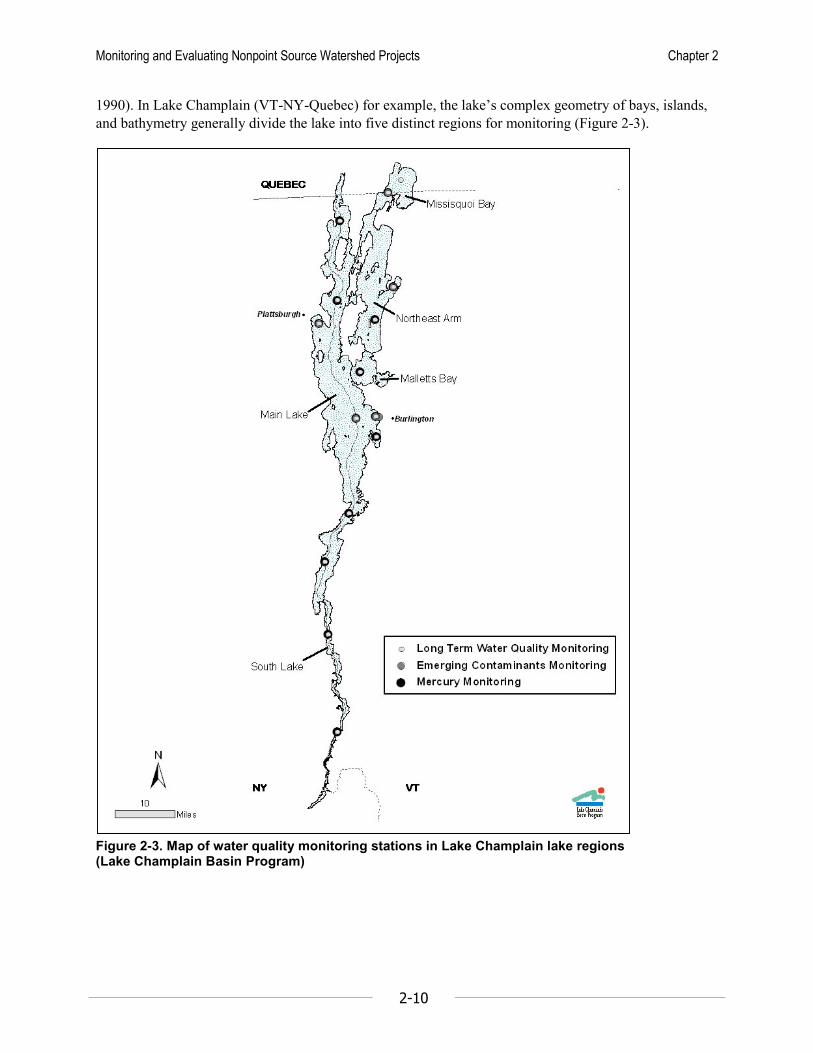
Wetlands can occur at numerous landscape positions (Figure 2-5) and are often classified according to differences in hydrologic conditions (source of water, hydroperiod, hydrodynamics), vegetation (emergent, shrub-scrub), topography (depressional, riverine), and to a lesser degree, soils (muck, peat, unconsolidated) (USEPA 2004). Within the context of assessing wetland condition, classification is intended to reduce variability within a class and enable more sensitivity in detecting differences among impacted and impaired wetlands within the same classification. Different classes of wetlands may be subject to different stressors and may vary in their relative susceptibility to particular stressors.
Figure 2-5. Wetlands and waterways of the Inland Bays watershed (DE CIB n.d.)
Due to the tremendous diversity among natural wetlands, a wetland monitoring program needs to be based on a specific wetland’s attributes. Strategies for designing an effective monitoring program build from a hierarchy of three levels that vary in intensity and scale, ranging from broad, landscape-scale assessments (Level 1), to rapid field methods (Level 2), to intensive biological and physico-chemical

Monitoring and Evaluating Nonpoint Source Watershed Projects Chapter 2
2-14
measures at Level 3 (USEPA 2004). One of the key considerations for wetlands monitoring is definition of the assessment area, whether it is the entire wetland or a portion of the wetland. Rapid assessment procedures have been shown to be sensitive tools to assess anthropogenic impacts to wetland ecosystems, and can therefore be used to evaluate best management practices, to assess restoration and mitigation projects, to prioritize wetland related resource management decisions, and to establish aquatic life use standards for wetlands.
USEPA’s 2006 Application of Elements of a State Water Monitoring and Assessment Program for Wetlands provides states with information to plan a wetland monitoring program and includes a discussion of the selection of indicators and metrics that reflect the unique characteristics of wetlands and their response to human-induced disturbance (USEPA 2006a). Several “modules” have been developed by EPA to support development of biological assessment methods to evaluate the overall condition and nutrient enrichment of wetlands (USEPA 2002b). These modules can be found at http://water.epa.gov/scitech/swguidance/standards/criteria/nutrients/wetlands/index.cfm.
Finally, because they are so biologically productive, wetlands tend to cycle sediment, nutrients, and other pollutants very actively among physical (e.g., sediment), chemical (e.g., water column), and biological (e.g., vegetation) compartments. Therefore, in a wetland monitoring program it may be important to look at each of these compartments, not treat the wetland as a simple input-output box. Moreover, because vegetation is a key element of wetland systems, seasonality of vegetation growth and senescence may be an important driver for nutrient cycling and therefore for monitoring design (USEPA 2002a).
2.2.1.4.4 Estuaries Estuaries differ from freshwater bodies largely due to the mixing of fresh water with salt water and the influence of tides on the spatial and temporal variability of chemical, physical, and biological characteristics. Incoming tides affect estuaries by pushing salt water shoreward while fresh water is entering from freshwater systems (Figure 2-6). Fresh water is lighter, so it flows over the top of salt water, while the tide forces the salt water shoreward and under the inflowing fresh water. Outgoing tides pull the entire water mass toward the ocean, and the freshwater input fills the gap left by the receding submerged salt water. These processes affect daily and seasonal salinity distributions.
Figure 2-6. Mixing of salt water and fresh water in an estuary (after CBP 1995)

Monitoring and Evaluating Nonpoint Source Watershed Projects Chapter 2
2-15
Because of the dynamic interaction of fresh water and salt water, pollutants are not flushed out from estuaries in the same manner as they are in most stream systems. Instead, an estuary often has a lengthy retention period (Ohrel and Register 2006). Consequently, waterborne pollutants, along with contaminated sediment, may remain in the estuary for a long time, magnifying their potential to adversely affect the estuary’s plants and animals. This retention period also introduces a lag time that must be factored into monitoring plans intended to measure improvements resulting from restoration or improved land management.
The unique characteristics of each estuary must be recognized and understood when developing a monitoring plan because of their impact on estuarine hydrology, chemistry, and biology. Basin shape, mouth width, depth, area, tidal range, surrounding topography, and regional climate all play important roles in determining the nature of an estuary (Ohler and Register 2006). The earth’s rotation (Coriolis effect), barometric pressure, and bathymetry (submerged sills and banks, islands) affect circulation and spatial variability in estuaries. For example, Puget Sound’s complex circulation pattern is driven by tidal currents, the surface outflow of freshwater from Puget Sound rivers, the deep inflow of saltwater from the ocean, wind strength and direction, and underwater sills (Gaydos 2009).
Freshwater inflow is a major determinant of the physical, chemical, and biological characteristics of most estuaries. It affects the concentration and retention of pollutants, the distribution of salinity, and the stratification of fresh water and salt water (NOAA 1990). These freshwater inputs typically vary seasonally. For example, Figure 2-7 shows how salinity in the Chesapeake Bay is generally higher in fall and lower in spring due to spring runoff (CBP 1995). Salinity and other characteristics of estuaries may also vary spatially due to the location of freshwater inflows. The temporal variability of estuary condition is also influenced by factors other than freshwater inputs. For example, temperature profiles vary seasonally, and tidal cycles can affect the mixing of fresh and salt waters and the position of the fresh water-salt water interface.

Monitoring and Evaluating Nonpoint Source Watershed Projects Chapter 2
2-16
Figure 2-7. Salinity in the fall and spring in the Chesapeake Bay (CBF n.d.)
2.2.1.4.5 Nearshore Waters The interplay of wind, waves, currents, tides, upwelling, tributaries, and human influences control water quality – and monitoring requirements – in nearshore waters. For the purposes of this guidance, nearshore waters include an indefinite zone extending away from shore, beyond the breaker zone (USEPA 1998); the term applies to both coastal waters and large freshwater bodies such as the Great Lakes. Wind and tides are the primary sources of energy in the coastal nearshore, and waves generated by the wind are largely responsible for currents (SIO 2003). These waves also have a central role in the transport and deposition of coastal sediments as well as the dispersion of pollutants and nutrients.
Upwelling brings cold, nutrient-rich waters to the surface, encouraging biological growth (Gaines and Airame 2010). Upwelling is extremely variable in space and time, depending on factors such as the strength and direction of the winds and the topography of the coastline (Gaines and Airame 2010). The spread of upwelled water down the coast of southern California can vary from a relatively narrow band near the coastline to enormous filaments extending hundreds of miles from shore. Upwelling on the east coast of Florida has been shown to be so dependent on the prevailing winds that it ceases as soon as the driving force is terminated (Taylor and Stewart 1959). Upwelling also occurs in the Great Lakes (Blanton 1975, Plattner et al. 2006). For the period 1992-2000, the magnitude of upwelling events observed in the southern basin of Lake Michigan tended to be greater than in the northern basin because the southern lake surface is typically warmer than in the north, while the temperature of the hypolimnion is more balanced

Monitoring and Evaluating Nonpoint Source Watershed Projects Chapter 2
2-17
over the extent of the lake (Plattner et al. 2006). In Lake Ontario, upwellings caused rapid shifts in the nearshore species composition of zooplankton and may be a mechanism for transport of certain diatom species to the epilimnion from hypolimnetic waters (Haffner et al. 1984).
Nearshore currents and pollutant transport are also affected by tributaries and human-made structures. Tributaries introduce fresh water to coastal waters and have varying potential to alter nearshore currents depending on factors such as tide stage, wind conditions, and tributary flow rate. Headlands (narrow strips of land that extend seaward), breakwaters (barriers built into the water to break the force of waves), and piers can influence the circulation pattern and alter the direction of nearshore currents (SIO 2003). For example, an obstruction on the down-current side of a linear beach will cause a pronounced rip current to extend seaward.
Current patterns must be sufficiently understood to determine the best locations for monitoring and to establish pollutant pathways and the likely relationships between land-based activities and nearshore water quality. Because circulation and pollutant transport is so variable in nearshore areas, designing monitoring plans based on assumptions about current patterns is not recommended. For example, a study of nearshore coastal circulation at the mouth of the Kennebunk River in Maine showed that currents did not carry river water directly to a local beach as expected (Slovinsky 2008); instead, river outflow extended much farther offshore from the beach. Because the current system of nearshore waters drives the relationship between land-based pollutant sources and receiving water quality, monitoring should include provisions to track variables needed to characterize the current sufficiently to aid interpretation of other chemical, biological, and physical data that are generated. Basic data on salinity, water temperature, and depth are often essential to identify the source of the sampled water and characterizing current patterns. The NOAA (U.S. Department of Commerce, National Oceanic and Atmospheric Administration) Great Lakes Coastal Forecasting System forecasts surface currents, winds, water temperature, and water level displacement, information that could be useful for sampling on any given date (GLERL 2011).
EPA, through its new Beaches Environmental Assessment, Closure and Health (BEACH) Program, is working with state, tribal, and local governmental partners to make nearshore water quality information available to the public. The BEACH Program provides a framework for local governments to develop equally protective and consistent programs across the country for monitoring the nearshore water quality along beaches and posting warnings or closing beaches when pollutant levels are too high. More information on this program can be found at http://water.epa.gov/type/oceb/beaches/beaches_index.cfm.
Note that because nearshore areas tend to be subject to heavy human use (e.g., swimming, boating, shellfish production), special water quality criteria and standards may apply. Fecal bacterial criteria for shellfish production, for example, tend to be far more restrictive than criteria for contact recreation. Such criteria may require special monitoring programs.
2.2.1.4.6 Ground Water Ground water is the source of much of the Nation’s streamflow, and ground water discharges often sustain water levels in lakes and wetlands, particularly during dry periods (Taylor and Alley 2001). The fact that the presence, quantity, and movement of ground water are not readily observable presents special challenges for monitoring design.
Ground water occurs in two general types of aquifers – confined and unconfined. Unconfined (water table) aquifers are in direct contact with the atmosphere through the soil and the elevation of the water table surface (i.e., depth to ground water). They fluctuate freely in response to changes in recharge and discharge (Figure 2-8). Confined (artesian) aquifers are separated from the atmosphere by an

Monitoring and Evaluating Nonpoint Source Watershed Projects Chapter 2
2-18
impermeable layer (USDA-NRCS 2003) and may be under pressure that results in a flowing (artesian) well if drilled into the aquifer. Perched water is held above the water table by an impermeable or slowly permeable layer below and is often the source of springs.
Figure 2-8. Basic aquifer types
Ground water levels are controlled by the balance among aquifer recharge, storage, and discharge (Taylor and Alley 2001). This balance is affected by characteristics (e.g., porosity, permeability, and thickness) of the rocks or sediments that compose the aquifer, as well as climatic and hydrologic factors (e.g., the timing and amount of precipitation, discharge to surface-water bodies, and evapotranspiration). Ground water moves along a hydraulic gradient from locations of higher hydraulic head to locations of lower hydraulic head. The rate of ground water movement depends not only on hydraulic head but also on the hydraulic conductivity (permeability) of the aquifer material; movement may be as rapid as 50 – 1000 m/day in a coarse gravel aquifer or as slow as 0.001 – 0.1 m/day in a silt and clay formation. The direction of ground water movement is not always obvious and not always consistent with the land surface topography. Patterns of ground water movement must be determined in the field (usually by measuring hydrologic head in numerous positions across a wide area) before determining sampling locations.
Ground water quality is influenced by a range of factors including aquifer type, native geology, precipitation patterns, flow patterns, land use, pollutant sources, and pollutant characteristics such as density and solubility (Scalf et al. 1981). Naturally, these factors can vary widely, even within a small region. A study of two adjacent Maryland watersheds with similar topography, land use and soils found that N yields differed significantly, largely due to the different characteristics of the aquifer underlying the watersheds (Bachman et al. 2002).
A special case of ground water systems is karst topography. Karst is a geologic condition shaped by the dissolution of channels or layers of soluble bedrock due to the movement of water. Karst regions typically display such surface features as sinkholes and disappearing streams and may be underlain by extensive cave systems. Aquifers in karst terrains are very sensitive to contamination because direct and rapid connections exist between the land surface and ground water, via the dissolution channels. Sinkholes are,

Monitoring and Evaluating Nonpoint Source Watershed Projects Chapter 2
2-19
for example, potentially direct pathways for sediment and chemicals to enter ground water without filtration through the soil. Karst systems present special challenges for ground water monitoring efforts, as sources of aquifer contamination may be widely dispersed and difficult to map.
The uncertainties regarding ground water flow patterns and the composition of underground materials, coupled with seasonal patterns and the interplay of surface water and ground water, require that basic knowledge of the particular ground water system under study be obtained before a monitoring program is designed or initiated.
Regional or statewide ground water level recording and water quality monitoring networks are common across the nation, especially in regions where ground water is a primary source of drinking and irrigation water (FACWI 2013). These networks often detect contaminants via well monitoring and model contaminant transport based on ground-water level data. Watershed-level monitoring of ground water, however, is still relatively rare despite the frequently important interaction between ground water and surface water. The interaction of surface water and ground water can be considered from the perspective of surface water recharging ground water or ground water discharging to a stream or lake (Goodman et al. 1996). The former is important when determining the impact of surface water on a ground water resource, whereas the latter should be a key element of monitoring when ground water comprises a significant portion of the water or contaminant budget of the surface water body (e.g., Schilling and Wolter 2001, Schilling 2002). When conducted well, ground water monitoring data, coupled with agricultural and land use data, can develop convincing evidence of the response of ground water quality to changes in agricultural management (e.g., Exner et al. 2010).
While the collection and analysis of groundwater data are not addressed in detail here, it is important that the role of subsurface waters be factored into watershed-scale and field-scale monitoring efforts described in this guidance. Several guidance documents are available for those seeking additional details regarding ground water monitoring, including guidance on construction of monitoring wells and sampling procedures (Scalf et al. 1981, Wilde 2006). The USGS has produced a series of groundwater technical procedures documents (GWPDs) that describe measurement and data-handling procedures commonly used by the agency in its groundwater monitoring activities (Cunningham and Schalk 2011). These procedures address groundwater-site establishment, well maintenance, water-level measurements; groundwater-discharge measurements, and single-well aquifer tests. In addition, guidance specific to monitoring ground water in NPS studies was developed based on experiences in the Rural Clean Water Program (Goodman et al. 1996).
Ground water monitoring is performed for a number of purposes, including:
To characterize background water quality.
To determine the ground water component of a hydrologic/chemical budget for a surface waterbody.
To document the impact of a polluting activity.
To identify trends and variations in water quality.
To determine the effectiveness of BMPs.
Successful ground water monitoring design begins with a good understanding of the ground water system and the establishment of specific monitoring objectives. Ground water monitoring often requires a two-stage approach in which the first stage is a hydrogeologic survey to determine ground water surface

Monitoring and Evaluating Nonpoint Source Watershed Projects Chapter 2
elevations and flow rates and directions. First-stage surveys require numerous sampling stations because aquifer water quality can vary considerably with depth and location (Figure 2-9). Ground water level data can be used to determine ground water flow patterns as shown in Figure 2-10 (Winter et al. 1998).
Figure 2-9. NO3 concentration versus depth to water table (after Rich 2001)
Figure 2-10. Determining ground water flow patterns (Winter et al 1998)
2-20

Monitoring and Evaluating Nonpoint Source Watershed Projects Chapter 2
2-21
The second stage is an investigation of water quality, with stations selected based on monitoring objectives and the results of the first stage (Goodman et al. 1996, USDA-NRCS 2003). Sampling locations can and should be guided by knowledge of the hydraulic gradient, but the heterogeneous nature of surbsurface environments makes appropriate location of sampling points a complicated and unpredictable task (Scalf et al. 1981). Several sampling locations and sampling from multiple depths may be required to characterize ground water and determine contaminant pathways (Goodman et al. 1996). Ground water investigations in South Dakota, for example, have shown that nested wells may be necessary for adequate examination of shallow aquifer water quality (SDDENR 2001).
In some cases it may be necessary to sample the unsaturated zone to get a true picture of the threat to ground water (Scalf et al. 1981, Goodman et al. 1996). In addition, long-term water level measurements may be needed to show how contaminants are transported from their sources through the groundwater system (Taylor and Alley 2001). It may even be possible to establish relationships between water levels and contaminant concentrations, possibly indicating patterns associated with seasons or rainfall-events.
Because ground water monitoring is both complex and expensive, sophisticated geostatistical techniques (e.g. Chiles and Delfiner 1999, Lee et al. 2005) are increasingly used both to build conceptual hydrogeological models of ground water flow, quality, and contamination and to assess health and environmental risk based on observed sample data (EPA Victoria 2006). Thus, modeling and spatial analysis can be useful in designing ground water monitoring programs and in organizing and interpreting results.
2.2.1.5 Climate Climate is one of the principal determinants of the basic structure of a monitoring program. The frequency, intensity, and duration of runoff-producing storm events affect sampling frequency and duration, equipment selection, automatic sampler programming, and many other elements of a monitoring program. Freezing conditions can have immense impact on the duration of the sampling season, the design and cost of permanent sampling stations, and the operation and maintenance of sampling equipment. Droughts and floods can be fatal to monitoring programs that have no budget flexibility, and the lag time between BMP implementation and measurable water quality impacts can be changed drastically by persistent changes in weather patterns.
Average precipitation patterns and the resulting average flow conditions are typically used to establish sampling frequencies, the relative emphasis on base-flow and storm-event sampling, the location of biological monitoring sites, and the design and siting of flow gaging stations. Precipitation patterns over any given study period, however, can vary significantly from long-term averages, as evidenced by a seven-year study in Illinois in which annual precipitation was lower than the long-term average in all but one year (Algoazany et al. 2007). An analysis of precipitation in the Minnesota River Basin for the period 1891-2003 showed a slightly increasing trend, with annual totals ranging from well under 400 mm to well above 900 mm (Johnson et al. 2009). In a runoff study on a dairy in the Cannonsville Reservoir watershed in New York, seven of the eight highest event flows occurred in the post-BMP period despite the fact that the pre- and post-BMP study periods exhibited similar scales and frequencies of precipitation and event flow volume (Bishop et al. 2005). Short-term and long-term drought greatly influenced runoff events in an 11-year study in Georgia (Endale et al. 2011). During the 86 months with below-average rainfall there were only 20 runoff events, compared to 54 runoff events during the 46 months with average or greater rainfall.

Monitoring and Evaluating Nonpoint Source Watershed Projects Chapter 2
2-22
Monitoring program managers must plan for a wide range of flow conditions, but flow is not the only important consideration when designing a monitoring program. Climatic variability can also influence aquatic organisms and land treatment programs. For example, the growth and development of riparian buffers is dependent on adequate precipitation. No monitoring program can be designed to handle all of the potential impacts of climatic variability, but all monitoring programs should be designed to account for a foreseeable range of conditions. Design concerns can range from determining the size of a flume required to measure edge-of-field runoff to planning budgets and time frames to allow the capture of a sufficient number of high-flow events.
2.2.1.6 Soils, Geology and Topography Soils, geology, and topography are local or regional features that must be considered in monitoring program design (MacDonald et al. 1991). These characteristics influence the hydrologic budget, potential suspended sediment loading from erosion, background levels of nutrients and dissolved ions in ground and surface waters, and other factors that drive monitoring program design.
The importance of soil groups is illustrated by a Pennsylvania study in which runoff was monitored from two contrasting hillslope soil groups (colluvial and residual) that differed in subsurface morphological characteristics such as the presence of a fragipan, the clay content of argillic horizons, and drainage class (Needelman et al. 2004). Results showed greater runoff from the four colluvial sites for all significant events, and overall runoff yields were also greater from the colluvial sites (average of 2.4 percent) than from the two residual soil sites (average of 0.01 percent).
A study of an agricultural watershed in the coastal plain of Maryland showed the importance of near-stream geomorphology and subsurface geology in determining riparian zone function and delivery of NO3
to streams (Böhlke et al. 2007). Stream NO3 levels were higher during high flow conditions when much of the groundwater passed rapidly across the riparian zone in a shallow, oxic aquifer wedge and higher during low flow conditions when stream discharge was dominated by upwelling from the deeper, denitrified parts of the aquifer.
Slope must also be factored into the design of a monitoring program because slope and slope length affect the rate and duration of runoff from a watershed, rate of erosion, depth of soil (steep slopes often have less soil overlying the bedrock), and stream characteristics. Slope also affects the likelihood of landslides and debris flow, erosional processes, and weathering rates.
2.2.2 Monitor Source Activities NPS pollution is highly variable and is generated by activities on the land that vary in location, intensity, and duration. To make the connection between pollutant sources and water quality observed through monitoring, it is also necessary to monitor the activities on the land that generate NPS pollutants. In the context of linking cause and effect, water quality monitoring data represent the effect, while source activities represent a major component of the cause. Put another way, to fully understand NPS pollution, we must measure both the dependent variables (water quality) and the independent variables (source activities).
In practice, monitoring pollutant source activities usually translates to land use and land management monitoring. This means more than taking a static picture of land use/land cover in a watershed from a satellite image (although that may be very useful for establishing a baseline condition). It means monitoring dynamic pollutant-generating activities in time and space. Examples of NPS pollutant types and common corresponding source activities to be monitored are shown in Table 2-2.

Monitoring and Evaluating Nonpoint Source Watershed Projects Chapter 2
2-23
Table 2-2. Selected NPS pollutants and watershed source activities to monitor NPS Pollutant Type Potential Variables to Monitor Suspended sediment (field erosion)
Cropland tillage, planting, harvesting, erosion control BMPs, precipitation.
Suspended sediment (streambank erosion)
Streamflow, stream morphometry, riparian condition, precipitation.
Phosphorus Manure applications, livestock populations, manure and fertilizer management, soil test P. Nitrogen Fertilizer applications, legume cropping, manure and fertilizer management, groundwater
movement. Crop herbicides Herbicide application rates and timing, precipitation Pathogens Livestock populations, grazing practices, riparian condition, pasture fencing, manure land
application practices. Pet populations, wildlife/waterfowl activity, septic system maintenance/failure, sewer maintenance, illicit discharge/connections.
Salt Amount and timing of road salt used for deicing. Road salt contract amounts. Miles and locations of roads salted. Irrigation return flows.
Heavy metals Vehicle traffic, highway infrastructure, street sweeping, stormwater management structures and activities.
Stormwater flow Impervious cover, stormwater management facilities, precipitation.
The practice of source activity monitoring is discussed in more detail in section 3.7 of this guidance.
2.2.3 Critical Details Execution of a monitoring plan requires careful attention to some critical details, as the following discussion reveals.
2.2.3.1 Logistics Logistics are defined here as matters concerning the management of the flow of materials, information or other resources from the point of origin to the point of use to meet the requirements of an enterprise. In water quality monitoring, logistics refers specifically to supporting the basic functions of data collection.
Supplying power to field stations.
Ensuring access to sampling locations for sample collection and field measurements.
Delivering, maintaining, and retrieving equipment, instruments, and supplies to and from the sampling sites.
Providing communications and data links between a base and remote sampling stations.
Having available, well-trained, and on-call field personnel.
Traveling to and from sampling stations.
Delivering samples to the laboratory on time and under appropriate chain of custody.
All of these elements must be addressed in the process of developing a monitoring plan. If necessary, how will power (direct AC, solar, or battery) be supplied? Can desired sampling locations be accessed legally and safely under the range of expected conditions (e.g., high flow, inclement weather)? If structures or shelters are necessary, can the property owner’s and municipality’s permission be obtained? What is the time and cost involved in traveling to and from a network of sampling locations? Is electronic

Monitoring and Evaluating Nonpoint Source Watershed Projects Chapter 2
2-24
communication between stations and a base (if desired) possible, considering distance and topography? Can samples be delivered to the laboratory within the limits of required holding times?
These and other practical questions of how to carry out the physical tasks of monitoring need to be considered in the planning stage. Some practical guidance for addressing such logistical issues is presented by Harmel et al. (2006).
2.2.3.2 Quality Assurance/Quality Control and the Quality Assurance Project Plan (QAPP)
Data collected by a monitoring program must be of sufficient quality and quantity – with respect to accuracy, precision, and completeness – to meet project objectives. Provisions for ensuring data quality must be made during the monitoring design process, not after a plan is underway. These provisions fall into two main categories. Quality control (QC) refers to a system of technical procedures developed and implemented to produce measurements of requisite quality. QC activities typically include the collection and analysis of blank, duplicate and spiked samples, analysis of standard reference materials, and inspection/calibration/maintenance of instruments and equipment. Quality assurance (QA) is an integrated system of management procedures and activities to verify that the QC system is operating within acceptable limits and to evaluate and verify the quality of data collected. A QA system addresses the roles and responsibilities of monitoring staff, required staff skills and training, tracks sample custody, sets data quality objectives and procedures for data validation, and monitors QC activities, including actions taken to correct problems. In general, each organization that conducts monitoring should ensure that the appropriate QA/QC measures are followed, but may vary among funding organizations.
All organizations conducting environmental programs funded by EPA are required to establish and implement a quality system, a structured system that describes the policies and procedures for ensuring that work processes, products, or services satisfy stated expectations or specifications (USEPA 2001). EPA also requires that all environmental data used in decision making be supported by an approved Quality Assurance Project Plan (QAPP) which documents the planning, implementation, and assessment procedures for a particular project, as well as any specific quality assurance and quality control activities (USEPA 2008b). The purpose of the QAPP is to document planning results for environmental data operations and to provide a project-specific “blueprint” for obtaining the type and quality of environmental data needed for a specific decision or use. In most monitoring programs, an approved QAPP is required before data collection can begin; even in cases where a QAPP is not specifically required, such a document is a valuable resource for documenting consistent monitoring procedures, and therefore useful to prepare even if not required. Quality control, quality assurance and the QAPP process are discussed in detail in chapter 8.
Other agencies including the United States Geological Survey (USGS) have issued guidance and requirements regarding data quality (Wilde 2005). Every USGS study requires a sampling and analysis plan (SAP) and a quality-assurance plan (QAP) that include a description of the objectives, purpose, and scope of the study and its data-quality requirements. In addition, each USGS Water Science Center develops general quality-assurance plans that articulate its policies, responsibilities, and protocols. Specific guidance on obtaining representative samples can be found in USGS’s National Field Manual (Wilde 2006). USGS quality control procedures emphasize generating information on bias and variability because of their importance in proper and scientifically defensible interpretation of collected data.

Monitoring and Evaluating Nonpoint Source Watershed Projects Chapter 2
2-25
2.2.3.3 Data Management and Record-keeping Even short-term monitoring efforts may generate tremendous quantities of data. A system for managing that data stream must be included in an overall monitoring plan. Poorly recorded, misunderstood or even lost data represent an irretrievable loss of information, a waste of resources, and a threat to program objectives. Poor data management can also make the task of data analysis and interpretation more difficult and challenging than necessary.
Good data management begins in the field, where a clear identification system is required to correctly attribute data to their source. Field log sheets or notebooks are valuable tools for initial recording of field data, sample identification and observations that may represent critical knowledge later. A good field log can also serve as a guide or checklist for the field technician.
Chain of custody records are essential where litigation is involved, but also useful for simply tracking delivery of samples to the lab. It is also important to document assignment of lab sample numbers and their correspondence to field identification codes.
The process and schedule of data reporting from the laboratory should be outlined and agreed upon. Timely reporting of data from the lab is essential in providing feedback to the monitoring and land treatment program.
A good data management system should be implemented in a simple, consistent format (e.g., a spreadsheet or a database form) that can accept both manually transcribed data (such as those from field logs or lab data reports) and data already in electronic form (such as downloads from field instruments or data loggers). Electronic data formats should be designed to be consistent with formats used for later analysis (e.g., in a statistics package or uploads to STORET) to avoid the cost and potential errors of transcribing data from one format to another.
Data validation and error checking are essential and should be performed at an early stage. Validation involves checking for correct transcription between data sources and data storage (e.g., between field logs and electronic spreadsheets), checking for typographic errors, looking for extreme or impossible values, and ensuring that all required data have been included. Validation should be performed on 100 percent of the data, not just a spot-check. It is very important that validation be performed early in the process, as it is costly and frustrating to have to repeat data analysis and presentation if errors are discovered late in the process.
Data storage is also an important consideration. Paper records such as field logs or lab data reports should be archived and perhaps scanned for electronic storage. Both original data and data derived from calculations, analysis or other manipulations should be stored. Maintain a metadata file to record important information about the data and the monitoring program, QA/QC results, exceptions or unusual occurrences, and any other important monitoring records. If data are stored in a national repository, such as STORET, download the data and make sure they are identical to the data on your desktop. Electronic data forms should be stored redundantly and protected with frequent backups. For long-term archiving, select the storage medium carefully. Data from a 1985 project stored on 5.25 inch (in) floppy disks may be nearly impossible to access in 2015; data recorded on a CD today may be unreadable in the future.
2.2.3.4 Roles and Responsibilities Most monitoring programs involve cooperation among several different agencies, offices or individuals. For example, a watershed project might include funding (USEPA), planning and implementation of BMPs (USDA-NRCS, Soil and Water Conservation Districts), flow measurement (USGS), water

Monitoring and Evaluating Nonpoint Source Watershed Projects Chapter 2
2-26
chemistry sampling and analysis (Health Department), and biomonitoring (state environmental agency). Even within a single activity, such as water chemistry monitoring, different individuals like field technicians, laboratory analysts and graduate students may play different roles. A good monitoring plan needs to specify the roles and responsibility of each participating entity and individual so that all monitoring tasks can be accomplished smoothly. Perhaps even more important, a mechanism for coordinating among the variety of agency and individual roles and responsibilities should be established from the start. Strong leadership from an overall project director/coordinator can facilitate good cooperation among a project team. In addition, frequent contact, progress reports, and regular meetings among all project participants have been shown to be key ingredients for effective coordination.
2.2.3.5 Review of Monitoring Proposals Monitoring plans may be developed and reviewed under a variety of different templates or formats. Whether for an internal check for completeness or for an external review in an approval process (e.g., for state Section 319 funding), it is often useful to step back from the details and review the contents of a monitoring plan to make sure that all necessary elements have been considered and addressed. Experience of NPS monitoring efforts across the country suggests that confirmation of the following elements is useful in review of monitoring plans:
Watershed Identification and Characterization
• Descriptive information on physiographic setting, water resources, land use/management
• Identification of stakeholders and project participants
Problem Identification
• Clear identification of water quality problem(s)
• Documentation of impairment(s) and supporting data
• Known or suspected causes and supporting data
• Known or suspected sources of pollutants and supporting data
Project Goals and Objectives
• Quantitative goals for water quality – Tied to impairment, restoration of use(s) – Including estimated load reductions as appropriate
• Quantitative goals for land treatment implementation
Land Treatment(s) to be Implemented
• Identify critical areas and measures to be implemented
• Justification for specific practices selected
• Schedule and interim milestones/indicators of progress
• Availability of funds, personnel, and other resources
Monitoring Plan
• Water quality – Design – Variables

Monitoring and Evaluating Nonpoint Source Watershed Projects Chapter 2
2-27
– Locations – Frequency and duration – Sample collection and analysis
• Land use/land treatment – process and responsibility
• Availability of funds, personnel, and facilities
Data Management and Analysis
Administration/Management/Coordination
Reporting, Communication, Stakeholder Involvement
Timetable and List of Deliverables
Budget
Note that this checklist addresses several elements such as those associated with land treatment that may seem to be outside the immediate realm of water quality monitoring, but these must also be considered and coordinated with other project activities.
2.2.4 Feedback Although implementation of BMPs on the landscape and monitoring water quality at various locations in the watershed may seem to be separate activities that can proceed independently, successful NPS watershed projects require effective coordination and collaboration among all activities. It is therefore important to facilitate feedback of data and other information among different components of a watershed project. For example, water quality monitoring staff should know where and when BMPs are implemented in the watershed, and land treatment implementation should be guided by water quality data where possible. Even within the monitoring program, it can be critical for biomonitoring staff to know the results of water chemistry monitoring to fully understand what they observe in the biotic community.
Feedback mechanisms should be built into a watershed project from the beginning, not left to chance or put off to the final project report. Frequent examination, presentation and discussion of monitoring data will keep all project participants informed. Regular review of field data and observations can provide evidence of events or conditions in the watershed that reveal small problems before they become large. Similarly, frequent examination of laboratory results can show evidence of analytical or QA/QC problems before they result in major data loss. Feedback between water quality monitoring and land treatment personnel can help fine tune BMP implementation to known water quality problems and can provide land-based data to improve understanding of observed patterns in water quality.
Feedback can be generated by requiring frequent reports (e.g., monthly) and meetings for all project participants. The reports and meetings can be brief and follow a simple formula, but by requiring all sectors to periodically compile, examine and present their data, feedback among all data streams can be guaranteed.
2.2.5 Limitations of Monitoring In practice, monitoring does not always answer all of the questions or achieve all of the objectives because:
Available resources may fall short of estimated costs.
Monitoring and Evaluating Nonpoint Source Watershed Projects Chapter 2
2-28
A large number of different situations/scenarios create too many alternatives to evaluate cost-effectively.
Socio-economic factors may require modification of monitoring or land treatment plans.
Watershed size, access or other features impose significant logistical limitations.
Water quality conditions (e.g., range of flows) are too variable to effectively monitor.
Appropriate data quality cannot be achieved (e.g., volunteer monitoring).
The actual desired response to treatment cannot be monitored due to flooding or other physical changes in the resource.
The magnitude of change expected to result from treatment, especially in context of background levels or contributions from other uncontrolled sources, is small.
Lag time between land treatment and water quality response exceeds the duration of monitoring.
Random or catastrophic events (e.g., intense storms or chemical spills) overwhelm response to treatment.
In principle, if a project cannot afford monitoring that can be reasonably expected to achieve objectives within the design parameters, it is recommended to forgo the inadequate monitoring that will not serve project needs but will drain budget resources. It may be possible to narrow the monitoring objectives, reduce the required precision, or reduce the scope of the monitoring effort to stay within budget, but such compromises must be made within the context of designing a plan that will meet stated objectives that help the project meet its goals. Modeling may be an effective alternative, especially when numerous alternative scenarios must be considered. However, note that proper model application (including calibration and validation) requires some data and considerable resources. See section 6.3 for ideas on how to integrate monitoring and modeling.
2.3 Monitoring Scale Selection
2.3.1 General Considerations The scale of a monitoring plan is the size of the area to be monitored, a spatial consideration. Selection of the appropriate scale depends on the study objectives, study duration, type of water resource monitored, the complexity of the project, and available resources (USDA-NRCS 2003). Monitoring scale is generally locked in with the selection of monitoring design.
The choice of scale affects monitoring costs, duration and logistics. The ability to isolate the factors of interest (e.g., BMP effectiveness, transport pathways) generally increases as scale decreases, but the transferability of results generally decreases as scale decreases. Monitoring a set of 1 x 3 m plots, for example, may yield good data on how cover crops reduce soil loss, but such data are very difficult to extrapolate to a watershed-scale because small plots do not always reflect field-scale runoff processes or watershed-scale transport and delivery processes. Analysis of long-term data collected in the Lake Erie basin showed that watershed size had a much greater effect on concentration patterns than on unit area loadings (Baker 1988). The greatest effect was on peak concentrations; as watershed size decreased, peak concentrations of sediments, nutrients, and pesticides increased (Baker et al. 1985, Baker 1988). Pollutant concentrations returned to baseline levels more quickly in smaller watersheds and streams. It was also determined that increasing proportions of the annual load occur in decreasing proportions of time as watersheds become smaller, but that the high rates of export from small watersheds are distributed into

Monitoring and Evaluating Nonpoint Source Watershed Projects Chapter 2
2-29
larger numbers of individual events compared to larger watersheds. Because of these occurrences, it takes more sampling effort to accurately measure the loads from a smaller watershed, and the likelihood of missing high export rate events is greater (Baker 1988).
2.3.2 Options Monitoring can be performed at scales ranging from national to single points, but the primary options for the types of NPS monitoring studies addressed in detail by this guidance are the watershed and BMP scales, the latter of which includes field and plot studies described by USDA-NRCS (2003). National and statewide (or regional) monitoring scales are only briefly touched upon here, and point-scale sampling is addressed primarily for explanatory variables. In fact, the data collected from point-scale sampling performed in support of the types of monitoring described in this guidance will generally be extrapolated to larger scales. For example, precipitation data collected at a single point may be applied to a rooftop to estimate flow volume handled by a green roof, or used to represent precipitation in either or both drainage areas in an above/below design. Soil samples collected at single points in a field may be combined for analysis to represent average conditions or analyzed separately with results interpolated to represent varying conditions for plot or field stations. Soils and precipitation data are generally used as explanatory variables in the statistical approaches discussed in chapter 7.
2.3.2.1 Statewide or regional Statewide monitoring designs generally emphasize larger streams and rivers, public lakes, and the outlets of watersheds. States usually locate some of their monitoring at sites gaged by the USGS to take advantage of the flow data. Some monitoring stations at key locations are equipped with automatic samplers or sondes for continuous monitoring, but cost and logistical constraints limit most monitoring efforts to the collection of grab samples, a few field measurements (e.g., temperature, DO, conductivity), and biological and habitat monitoring. With the exception of the few stations with automatic or continuous sampling, monitoring frequencies are generally low.
Statewide monitoring associated with NPS pollution is generally designed to assess current conditions. It is unlikely that most statewide monitoring efforts can support trend analysis because of the strict requirements (e.g., no breaks in the data, consistent methods over time, collection land use and other covariate data) and the difficulty states have committing to consistent long-term monitoring efforts. Recognizing this and related limitations, Congress in 2005 began appropriating additional funds within Section 106 grants for an initiative to enhance monitoring programs and provide statistically-valid reports on water conditions (USEPA 2006b). In 2008, EPA amended its guidelines for this initiative to provide incentives for states to implement state-wide statistically-valid monitoring surveys (USEPA 2008a).
2.3.2.2 Watershed Watershed-level monitoring for NPS assessments and the evaluation of project effectiveness has evolved over the years as lessons have been learned from such programs as the Rural Clean Water Program (USEPA 1993a), ACP-Special Water Quality Projects (Davenport 1984), Model Implementation Program (NCSU and Harbridge House 1983), Nationwide Urban Runoff Program (USEPA 1983), and the Section 319 National NPS Monitoring Program (Tetra Tech n.d.). The current emphasis on Total Maximum Daily Loads (TMDL)s has changed watershed-level monitoring even further by placing a greater focus on estimating the pollutant loads from each source category in the watershed, setting numeric targets for pollutant load reductions at a watershed level, and linking NPS and point source control efforts (USEPA 2012a).

Monitoring and Evaluating Nonpoint Source Watershed Projects Chapter 2
2-30
Watershed-level monitoring can be triggered by findings from state-level monitoring, but is even more likely to develop from local stakeholder efforts to identify and solve problems that they care about (USEPA 2012b). Infrequent grab samples, basic chemical and physical parameters, and rapid assessments of aquatic biology conditions typically constitute the monitoring performed prior to or in the initial stages of a watershed project (USEPA 2008b). Flow data are generally lacking unless the watershed has a USGS gaging station, and monitoring stations are usually located where convenient for sampling, a situation that can bias results.
As watershed projects evolve, the monitoring approach should change to address project goals (USEPA 2008b). Initial efforts generally focus on refining the problem definition, including characterizing the water quality problem better, determining the major sources and causes of the problem, and providing data to aid in the design of a plan to solve the problems. Monitoring during this phase of a watershed project may include a synoptic survey, tests for toxicity, flow measurements at various points in the watershed to support a load analysis, detailed habitat assessments, and higher level biological assessments. Land use mapping, investigation of permitted discharger reports, and windshield surveys may also take place to better characterize sources. Most of the monitoring during this phase of a watershed project is short-term, with one or two sampling events at most. In rare cases, projects may install “permanent” monitoring stations and factor long-term monitoring considerations into the short-term effort. Such projects should ensure that all design requirements for long-term monitoring can be met, however, before monitoring begins.
Watershed-level monitoring, as described in this guidance, typically begins after a watershed project secures funding to address the identified problems. All too often project implementation begins before or simultaneously with monitoring, complicating efforts to assess the effectiveness of the project. The watershed monitoring plan should be coupled with and complementary to the watershed project or management plan (USDA-NRCS 2003). Depending on the specific objectives, the size and characteristics of the watershed, and the parameters of concern, watershed-level monitoring can take various forms. A key difference between watershed- and state-level monitoring is the narrowing of focus and increased intensity of watershed-level monitoring. Because the questions to be addressed by monitoring are more specific at the watershed level, each watershed monitoring effort is unique.
Watershed-level monitoring to assess project effectiveness generally requires a control condition to serve as a benchmark. This is not unlike the use of reference conditions for biological monitoring, but whereas reference conditions are generally sought in areas with minimal human impact (see chapter 4), the control conditions for watershed-level monitoring are usually found within or very near to the watershed being treated. In some cases, watershed projects will have relatively pristine conditions that serve as the control, but usually the control is an upstream area or a paired watershed within a short drive of the treatment watershed. Data from the control are used to isolate the effects of the BMP implementation in the study or treated area. This type of monitoring is not generally performed in statewide monitoring programs.
Another approach used at the watershed level is long-term trend monitoring at a single station where there is no control condition to serve as a benchmark. As described in section 2.4.2.5 and noted above for statewide monitoring, this approach has a relatively high risk of failure because the requirements of the method are difficult to satisfy over the long term. When performed at the watershed level, rather than the statewide level, however, the risk of failure can be reduced because more frequent sampling is done (e.g., once per two weeks) and the timeframe for demonstrating results is shortened. Still, the risk of failure with this approach remains generally greater than for designs using controls because the timeframe for monitoring at the watershed level can still be on the order of a decade.

Monitoring and Evaluating Nonpoint Source Watershed Projects Chapter 2
2-31
One of the biggest challenges at this scale is to determine when a watershed is too large for successful monitoring (USDA-NRCS 2003). The upper limit on watershed size will depend on the monitoring objectives. For trend analysis, there may be no upper size limit if monitoring will continue for decades. If the goal is to attribute trends to changes in land use or land management, the cost of tracking such information at a sufficient level of detail may be prohibitive for extremely large watersheds that cover 100,000 acres or more (~40,500 ha).
Problem assessment can be done at various levels of detail for various purposes. If the assessment is to form the basis for an action plan that will require the obligation of substantial resources, it may be wise to limit the monitored watershed size to 50,000 acres (~20,200 ha) or less (i.e., the HUC-12 level). If, for example, the watershed or basin plan is for an area of 500,000 acres (~202,000 ha), monitoring would be performed at ten subwatersheds of 50,000 acres each. Watersheds larger than 50,000 acres are considered very large and may be inappropriate for assessment monitoring because of their likely heterogeneity in land uses (USDA-NRCS 2003).
Pollutant load measurement can be performed at watersheds of any size, but attribution of those loads to specific sources or source categories becomes more difficult for large watersheds. A limit of 50,000 acres may be appropriate for load estimation within the context of watershed plans or TMDLs where load and wasteload allocations will be made. The exact size limit for any situation will depend on a wide range of factors including whether or not watershed modeling is part of the effort.
The appropriate watershed size for evaluating watershed projects is probably 25,000 acres (~10,000 ha) or less based on experiences in the NNMP and RCWP. The actual size depends on a number of factors including average annual precipitation, the type and degree of use impairment, lag time, study duration, the potential for making improvements with BMPs, the number and location of monitoring stations, and sample type and frequency.
In comparison to statewide monitoring, watershed-level monitoring generally involves a shorter timeframe (3-10 years), fewer stations, more frequent sampling of both storm events and base flow, and a targeted and unique set of monitoring variables. Flow is usually measured in watershed-level monitoring. Due to automation of monitoring stations, primarily to monitor storm events, the annual cost per monitoring station is generally greater than routine grab sampling programs. On the other hand, biological data are typically collected only once or twice per year, and as a result, the timeframe for demonstrating results is quite dependent on the specific problem identified and the treatment plan designed to solve the problem. Where stream and habitat restoration has been done in watershed projects, biological monitoring has often been successful in documenting benefits, but in the various, long-term, watershed-based NPS monitoring programs listed above (e.g., Rural Clean Water Program), there have been very few instances where biological monitoring has demonstrated the effectiveness of watershed projects that did not involve such in-stream work. As a result, this guidance recommends that biological monitoring be coupled with physical/chemical monitoring of the stressors targeted in watershed projects.
2.3.2.3 BMP or practice Monitoring at the BMP level is generally the most intensive of the levels described here. The scale for BMP monitoring can vary from plot studies to the inflow and outflow of a multi-acre constructed wetland to the influent and effluent of a manufactured stormwater treatment device. Monitoring variables are selected based upon the specific sources treated by the BMP, including such possibilities as metals and organic chemicals in an urban setting; bacteria and BOD near shellfish beds or livestock operations;

Monitoring and Evaluating Nonpoint Source Watershed Projects Chapter 2
2-32
nutrients and sediment on cropland; temperature, DO, and biological communities for a stream restoration; and pH in abandoned coal mining areas. Flow needs to be monitored in most BMP studies.
BMP-level monitoring is generally storm-event driven, with little or no base-flow sampling. Exceptions include monitoring of constructed wetlands or wet ponds where it is essential that time-of-travel is assessed to provide for “matching” inflow and outflow samples to estimate pollutant removals. In addition, monitoring of stream restoration often includes both storm events and base flow. Each condition presents a different combination of stressors on the biological community that is typically monitored for such projects.
While sampling is frequent and the schedule hectic, the duration of BMP-level monitoring is usually short, typically ranging from one to two years to no more than five years. Paired studies, random block designs and similar research-type study designs are often used when inflow-outflow monitoring is not possible. The intent of these studies is to eliminate all factors other than the BMP itself, so samples are collected as close as possible to the BMP.
Composite samples are collected in many BMP studies, but because it is often desirable to assess contaminant levels at different stages of the hydrograph, BMP studies may include analysis of several samples per storm event. BMP monitoring is often more expensive per site than either statewide or watershed monitoring.
2.3.2.3.1 Plot The plot scale is generally used in monitoring designs that feature replication, particularly for research objectives. This scale is not appropriate for problem assessment, pollutant load estimation, or trend analysis but can be used for preliminary assessment of the effectiveness of BMPs.
Monitoring at this scale will focus on storm-event monitoring, generally requiring automatic samplers, continuous flow measurement, and considerable annual expense. Rainfall simulation is often used at this scale to control study conditions. Monitoring duration is generally less than three years (USDA-NRCS 2003).
2.3.2.3.2 Field Field scale study units are larger than individual plots but can vary considerably in size (USDA-NRCS 2003). Field scale studies in urban settings include parking lots, rooftops and street segments. In agricultural settings, field scale studies include cropland field segments, paddocks and barnyards. A key characteristic of most field studies is that samples are taken from episodic runoff, not from waterbodies.
Monitoring at the field scale is useful for the following objectives:
Problem assessment, especially source characterization.
Load allocations.
BMP effectiveness.
Field scale monitoring is not recommended for trend analysis or determining the effectiveness of watershed projects.
Monitoring at this scale is usually completed in less than five years, and studies of individual BMPs can be completed in three years or less. Sampling is typically focused on storm events, with either discrete or

Monitoring and Evaluating Nonpoint Source Watershed Projects Chapter 2
2-33
composite sampling depending on the specific needs of the study. Flow measurement is essential to most field scale monitoring plans.
2.3.2.4 Summary Table 2-3 matches monitoring objectives with the appropriate monitoring scale. The best scales for assessing BMP effectiveness are plot and field, whereas the watershed scale is best for evaluating watershed projects. Both field and watershed scales can be useful for problem assessment and load estimation, whereas the watershed scale is generally best for trend analysis.
Table 2-3. Monitoring scale as a function of objective
Scale
Objective
Problem Assessment TMDL Loads Trends
BMP Effectiveness
Watershed Project
Evaluation Plot Χ Field Χ Χ Χ Watershed Χ Χ Χ Χ
2.4 Monitoring Design Selection
2.4.1 General Considerations As discussed above, monitoring objectives drive decisions on the details of a monitoring program. There are several experimental designs that can be applied to meet monitoring objectives, and some of the choices are obvious. All else being equal, the monitoring design selected should be the one that best matches available resources and presents the fewest logistical obstacles. Although this may seem obvious, it is important that monitoring design be determined before monitoring begins to ensure that suitable data are collected to meet monitoring objectives. Our discussion addresses monitoring design as a direct function of monitoring objective, modeled after guidance developed for agricultural monitoring projects (USDA-NRCS 2003).
2.4.2 Design Options The design options discussed in this section are:
Reconnaissance or synoptic
Plot
Paired
Single watershed before/after
Single-station long-term trend
Above/below
Side-by-side
Multiple
Input/output

Monitoring and Evaluating Nonpoint Source Watershed Projects Chapter 2
2-34
All of the above designs are targeted designs, which are the most common type of design used to evaluate BMPs or plan and evaluate watershed projects. With the exception of the input/output design, all of the designs are applicable to biological monitoring; however, the discussions that follow focus on the measurement of chemical and physical parameters via in-stream measurements and the collection of water samples. Chapter 4 provides more discussion on biological monitoring and provides some discussion on probabilistic designs, which are particularly useful for providing unbiased assessments of conditions in a waterbody or across a large geographic area. Section 2.5 of the 1997 guidance (USEPA 1997) also provides a detailed discussion of probabilistic monitoring designs. Detailed discussions of statistical tests recommended for each design can be found in chapter 7.
2.4.2.1 Reconnaissance or Synoptic Reconnaissance or synoptic studies are designed to provide a preliminary, low-cost overview or summary of water quality conditions in the area of interest. Reconnaissance surveys are often used to (USDA-NRCS 2003):
Determine the magnitude and extent of a problem.
Obtain preliminary data where none exist.
Target critical areas.
Data collected from reconnaissance surveys are generally used in the problem assessment and planning phases of watershed projects but can also be used to help design projects to evaluate BMPs. Reconnaissance surveys typically involve a relatively large number of sampling sites distributed across the study area, low sampling frequencies (e.g., one or two samples at each site for high/low flow or seasons), a core set of common monitoring variables with or without additional variables (e.g., pesticide scans) selected based on knowledge of specific problems or sources, and a short study duration (e.g., completed in under 12 months) (Figure 2-11). A common strategy is to sample significant tributaries, longitudinally along primary streams, and at locations indicative of selected land uses (including undisturbed).
Permanent monitoring stations are not installed for reconnaissance surveys and grab sampling is typically used. Integrated grab samples, sediment samples, the use of multi-parameter probes, and instantaneous flow measurements may be part of the sampling scheme depending upon the purpose of the study.
Because sample sizes are generally small, statistical analyses are not usually performed on reconnaissance data. Instead, it is common to gather all potentially useful data on water quality and land use and management, summarize the data in graphic or tabular form, and then interpret the data using best professional judgment. For example, pollutant concentrations can be plotted against water quality criteria to identify potential problem areas. Water chemistry data might be examined to see where pollutant concentrations are highest and lowest and whether any patterns might exist along the course of a stream or in tandem with patterns found in biological monitoring data. By superimposing water quality data summaries on top of a land use map, it may be possible to identify critical areas where BMPs are needed, particularly in cases where information has also been gained from visual surveys.

Monitoring and Evaluating Nonpoint Source Watershed Projects Chapter 2
2-35
Figure 2-11. Reconnaissance sampling design
2.4.2.2 Plot Plot studies are often used to:
Assess soil conditions including nutrient levels.
Assess pollutant transport pathways.
Determine the effects of BMPs on pollutant transport.
Plot studies are typically used in research and are sometimes established to provide information that is important to a broader watershed study. For example, the effectiveness of agricultural drainage water management practices, which is important to the broader Mississippi River Basin nutrient management effort (MRGOMWNTF 2008), could be addressed with plot studies. The ability of catch or cover crops to reduce N loading to the Chesapeake Bay is another example of a research question that could be addressed with plot studies. Findings from the plot studies could be incorporated into planning and modeling efforts for the large basins.
Nonpoint source plot studies typically employ a randomized complete block design or other, more complicated statistical design such as the Latin square and split-plot designs, or a factorial arrangement of treatments (USDA-NRCS 2003). Blocking is the arranging of study plots in groups (blocks) that are similar to one another (e.g., slope, soils, pavement type). The blocking factor is generally a source of variability that is not of primary interest to the investigator. The study plots within each block include a control and a treatment that is of primary interest such as different levels or forms of nutrient application, different cover crops, different levels of crop residue, or different street sweeping frequency. Each set of

Monitoring and Evaluating Nonpoint Source Watershed Projects Chapter 2
2-36
treatments is generally replicated at least three times, and each block is considered a replicate. The number of plots required for the study is:
Plots = t×b
Where t = number of treatments including the control b = number or blocks
Data from plot studies are typically analyzed using analysis of variance methods which are described both in chapter 7 and in chapter 4 of the 1997 guidance.
Plot studies using randomized complete block designs are common in the literature (Lentz and Lehrsch 2010, Wilson et al., 2010). Runoff plot studies usually require construction of permanent monitoring stations equipped with weather stations, automatic sampling equipment, and continuous flow measurement devices. In some cases remote access is provided. Samplers may be programmed to collect either discrete samples over the course of individual storm events or composite samples. Sampling is intensive and storm-event based, but studies are generally completed in three or fewer years.
Advantages of plot studies include the use of replicates and tight experimental control, but the results of plot studies are not generally widely transferrable (USDA-NRCS 2003).
2.4.2.3 Paired Paired-watershed design is the most powerful design option that is used with any frequency to evaluate the impacts of BMPs or projects (USDA-NRCS 2003, USEPA 1993b, Hewlett and Pienaar 1973). It has been used with success in a number of Section 319 NNMP projects, including Jordan Cove, CT (Clausen 2007) and Morro Bay, CA (CCRWQCB and CPSU 2003). The basic design requires two watersheds (treatment and control) and two time periods (calibration and treatment) as illustrated in Figure 2-12, but the design can include more than one treatment watershed. The discussion here is limited to a two-watershed design. Paired samples are collected from both watersheds during the calibration period and regression analysis is used to test for a relationship between the paired samples (USEPA 1993b). After the calibration period relationship is established, BMPs are implemented in the treatment watershed, paired samples are collected, and a new relationship is established between paired samples collected during the treatment period. At the end of the treatment period, the significance of the effect of the BMPs is determined using analysis of covariance (see section 7.8.2). A helpful narrated video describing the paired-watershed design can be found at the Jordan Cove, CT project website (Dietz 2006).
A variation on the paired-watershed design is the nested-paired-watershed design in which both monitoring stations are located in the same watershed (Hewlett and Pienaar 1973). In this design, it is preferred that the upper sub-watershed is used as the control, and the lower portion of the watershed is treated. This alignment will reduce the chances that the treatment basin will influence the control as the treatment effect passes through it (Hewlett and Pienaar 1973). The nested-paired watershed design is essentially equivalent to the above/below-before/after design described in section 2.4.2.6.
Selection of Paired Watersheds • Similar size and location • Similar slope, soils, and land cover • Similar runoff and base flow patterns • Similar relationships between
monitored variables and flow • Ability to control and document land
use and land treatment in both watersheds

Monitoring and Evaluating Nonpoint Source Watershed Projects Chapter 2
2-37
The first step in establishing a paired study is the selection of two watersheds or study areas that are likely to have qualitatively similar responses to precipitation events. This means that both watersheds will generally have runoff when it rains, base or no flow in the absence of runoff events, and a relationship between the concentrations of measured variables and flow. If these general responses to precipitation patterns differ significantly, good calibration may not be possible. Several attempts at paired studies have failed because the watersheds could not be calibrated. Choosing watersheds that are similar in size, slope, location, soils and land cover will increase the chances of selecting a good pair (USEPA 1993b).
Figure 2-12. Paired sampling design
Note that the control watershed can either be in a similar impaired condition as the treatment watershed or in the improved condition desired for the treatment watershed. In the first case, the expected result is that conditions in the treated watershed get better than in the control watershed, whereas in the second case the expected result is that conditions in the treated watershed become more like those in the control watershed. In VT, for example, Meals (2001) successfully used a highly-impaired agricultural watershed as a control, measuring the beneficial effects of treatment against that watershed. The essential characteristic of a control watershed is that it does not receive BMP treatment during the life of the monitoring project.
After a suitable pair is found, the next important hurdle is to ensure that land use and land treatment activities at both watersheds can be documented and controlled through study’s duration. Too often investigators have achieved control over the “treatment” watershed without securing equivalent control over the “control” watershed, only to find that activities in the control watershed (e.g., housing developments springing up on cropland or voluntary adoption of the BMPs under study) have compromised the study.

Monitoring and Evaluating Nonpoint Source Watershed Projects Chapter 2
2-38
The New York NNMP project successfully paired a dairy farm watershed with a forested watershed, but concluded that it was important to include matched measurements of flow volumes, and farm watershed measurements of event peak flow and event flow rate to account for inherent differences in watershed characteristics and hydrologic response in the analysis of P load data (Bishop et al. 2005). A forested watershed was selected as the control watershed because no significant changes were expected, as opposed to a farmed watershed where operational practices could be modified or the farm could go out of business during the 8-year study period.
Monitoring for paired studies can range from biological monitoring to grab sampling to automated sampling with permanent monitoring stations. Given the difficulty associated with orchestrating paired studies at the watershed scale, it is recommended that higher-level biological and/or automated sampling be performed to ensure collection of robust datasets. Well-designed paired studies can generally be completed in five to seven years. Projects can be extended or even interrupted in cases where BMP implementation is a lengthy process.
Advantages of this design for evaluating the effectiveness of BMPs and projects include control for hydrologic variation and inherent watershed differences and the potential for clear attribution of water quality response to the BMPs. It is also possible to examine the magnitude of the treatment effect for large versus small events or baseflow conditions, but this study requires adequate sample sizes for each data subset (Lewis 2006). Further, as demonstrated by the New York NNMP project, water quality monitoring can be suspended during BMP implementation without compromising the study design (Bishop et al. 2005). This can help address the problem of diluting the overall effect of treatment by lumping together data collected during the treatment implementation with post-treatment data (Lewis 2006). Land management tracking in both the control and treatment watersheds is recommended during BMP implementation to aid in data interpretation after water quality monitoring is resumed. Depending on the location of monitoring stations, pollutant loads estimated from paired studies could be used to support TMDLs.
Based on the NNMP experience, the greatest practical disadvantage of the paired design is the difficulty finding pairs, particularly at the watershed scale. Even when pairs are found, it is often difficult to control both watersheds, so land use and land management changes occur where and when needed to support the study. This challenge becomes even greater if multiple treatment watersheds are included in the design. A disadvantage of paired studies versus multiple-watershed studies is the conclusions pertain only to the specific watersheds and treatments tested; there is generally no practical ability to predict effectiveness of the treatments or differing levels of treatment in other watersheds from the same population (Lewis 2006). This disadvantage is because descriptors of the treatment (e.g., percent impervious area or percent of cropland in no-till) are generally not included in the statistical model tested.
2.4.2.4 Single Watershed Before/After In this design, a single monitoring station is located at the outlet of the study area. Sampling is performed before and after the implementation of BMPs. In watersheds subject to TMDLs, this design may be considered to measure pollutant loads before and after implementation of the TMDL to determine if loads have been reduced or TMDL load targets achieved. Typically the investigator is expecting to detect step changes in the target parameter with the monitoring program.
This design is not recommended for BMP effectiveness studies because there are no control stations (as in the paired design described earlier); and BMP effectiveness cannot easily be distinguished from other confounding effects (USDA-NRCS 2003). For example, if the “before” years are relatively dry and the
Monitoring and Evaluating Nonpoint Source Watershed Projects Chapter 2
2-39
“after” years are relatively wet or vice-versa, the differences in water quality and loads could be due to differences in weather rather than the effects of implemented BMPs. Generally, this design does not collect data that can be used to directly separate the effects of the BMPs from those of climate and is therefore a poor choice for assessing the effectiveness of BMPs or watershed projects. However, in the case of TMDLs, it would remain possible to compare measured loads versus target loads to see if goals have been achieved although attributing success or failure to TMDL implementation would be difficult. A possible exception would be the fortunate situation where water quality improved and pollutant loads were reduced despite increased runoff during the “after” years.
While this design is generally not recommended for BMP effectiveness studies, analysis of covariance (see section 7.8.2) can be used to provide some indication of BMP effects (USDA-NRCS 2003). Under this approach, a water quality variable could be related to a climate variable such as precipitation using a method described by Striffler (1965). A change in this relationship could be attributed to the BMP, but there would be no direct estimate of reduction of the water quality variable of interest. This approach would require a longer calibration period and results are not transferable to other areas (USDA-NRCS 2003).
Depending upon the study purposes, single watershed designs may or may not require construction of permanent monitoring stations, weather stations, automatic sampling equipment or continuous flow measurement devices. For some applications, grab samples will be sufficient, whereas composite sampling with automatic samplers will usually be needed in applications that require pollutant load estimation.
2.4.2.5 Single-Station Long-Term Trend This design has been a staple of water quality monitoring for decades and can be used to determine changes in water quality or pollutant loads over time. Single-station trend monitoring generally cannot be used to determine if BMPs improve water quality unless a very long water quality and concurrent land use/treatment monitoring program can be sustained.
Trend monitoring is similar to single watershed before/after monitoring except that there is no planned before/after period and the study duration is expected to be much longer (decades versus years). Advantages of this design include the single monitoring station, wide applicability, and the ability to account for lengthy lag times (see section 6.4) and gradual implementation of BMPs (USDA-NRCS 2003). Because of the expected longer study durations, additional considerations may be necessary due to major land use changes and data gaps; long-term commitment of resources; consistency in sampling and analytical methods over time; and tracking land use, land treatment, precipitation, and flow.
Simple statistical analyses can be used to detect trends; however, they do not indicate why the trend exists. Adjusting the trend data set for hydrologic influences can help in that regard. For example, using streamflow as an explanatory variable, it was possible to document a statistically significant reduction in sediment and TP load in Willow Creek, Michigan, storm runoff over the eight years of monitoring (Suppnick 1999). These reductions were then correlated with the percent of land in no-till.
See Meals et al. (2011) and chapter 7 for additional information on trend analysis.
2.4.2.6 Above/Below Above/below monitoring has been used with success to assess the water quality impact of isolated sources and determine the effectiveness of BMPs at isolated sources.
In this method, design stations are located upstream (or up-gradient) and downstream (or down-gradient) of the area or source that will be treated with BMPs (Figure 2-13). When used in the planning phase of a

Monitoring and Evaluating Nonpoint Source Watershed Projects Chapter 2
2-40
watershed project, grab samples and instantaneous flow measurements for one or two sampling events may be sufficient, but in most cases permanent monitoring stations are constructed and equipped with automatic sampling equipment, continuous flow measurement devices, and sometimes remote access. Depending on study objectives and flow conditions, samplers could be programmed to collect discrete samples over the course of individual storm events, weekly composite samples, or some other variant. Weather stations are usually included, but one station is often sufficient for both sampling sites. Study duration for evaluating BMP effectiveness is generally three to five years, but potentially longer for larger areas with multiple sources treated with a range of BMPs.
Samples are “paired” in this design, with the intent to sample the same unit of water when it is above and then below the study area. If monitoring is performed both before and after the BMPs are implemented (above/below-before/after design), this design becomes equivalent to a nested-paired-watershed design and can be treated statistically as if it were a paired-watershed design (see 2.4.2.3).
Figure 2-13. Above/below sampling design
Advantages of this design include:
It is widely applicable.
It is not as vulnerable to climate variability as the single watershed design.
It is useful for isolating critical areas in the watershed.
It can use the same statistical procedures (e.g., analysis of covariance) as a paired-watershed design because monitoring is performed before and after BMP implementation.
Load measurements can be useful in TMDL watersheds depending on station location.
A significant disadvantage of this design is the potential for upstream conditions (e.g., high stream temperatures or pollutant concentrations) to overwhelm downstream conditions, masking both the inputs of the isolated source or area and the effects of the implemented BMPs. This risk can be addressed by ensuring the isolated area contributes substantially to the downstream flow, but this may not be feasible without

Monitoring and Evaluating Nonpoint Source Watershed Projects Chapter 2
2-41
sacrificing the extent of the area is isolated. It is recommended that a reconnaissance effort be undertaken with sampling at both low flow and high flow conditions to see if the site is suitable for this design.
Other disadvantages include the possibility that inherent differences between the two stations (e.g., geology) or interactions between the BMPs and the watershed could be causing the measured differences in water quality (USDA-NRCS 2003). Monitoring before and after BMP implementation can help to address these issues. Absent complete knowledge of the interaction between subsurface and stream flows, there is always the risk that unsuspected sources are impacting downstream water quality as was found in the Maryland Section 319 National NPS Monitoring Program (NNMP) project where it was determined that ammonia from the upper portion of the watershed passed through nitrifying zones and was converted to NO3, thus elevating NO3 levels at the outlet of the watershed (Shirmohamadi et al. 1997, Shirmohammadi and Montas 2004). A major ramification of this discovery was that nutrient management had to be added to dairy manure management and stream fencing both as a BMP needed to solve the nutrient problems in the watershed and as a factor influencing stream N levels.
2.4.2.7 Side-by-Side Before/After Monitoring watersheds that are adjacent to each other without calibrating paired samples before treatment is equivalent to having two separate single-watershed studies as described under section 2.4.2.4. This design is not recommended for evaluation of BMPs or watershed projects because it is highly likely that there will be no way to distinguish among causal factors such as BMPs or land treatment, inherent watershed differences, or an interaction between BMPs and watershed differences (USDA-NRCS 2003).
2.4.2.8 Multiple Where resources allow, monitoring of multiple watersheds (or fields) may be used to demonstrate the effectiveness of BMPs (USDA-NRCS 2003). This design requires that more than two watersheds are selected for monitoring within the geographic area of interest. Two different treatments and perhaps a control are replicated across the monitored watersheds in roughly equal numbers. Treatments may already be in place when the study begins or may be implemented after a pre-treatment monitoring period. An effective design would typically include monitoring over several years.
One advantage of using this approach with a large number of monitored watersheds (e.g., 10 or more) is that variability among watersheds can be estimated. Furthermore, observing water quality changes of similar direction and magnitude occurring with land treatment changes across several watersheds serves to substantiate the evidence for BMP effectiveness and robustness of the BMP over a range of watershed conditions. A major problem with this design is the practical limitations and cost associated with controlling and monitoring many watersheds or fields. It is possible, however, that the increased annual sample size associated with the inclusion of multiple watersheds could reduce the overall timeframe for monitoring.
Lewis (2006) describes a multiple-watershed approach in which 3 of 13 watersheds are used as controls, 5 are fully treated, and 5 are partially treated. He argues that this design has a significant advantage over paired-watershed studies in that it allows for prediction under different conditions or treatment levels, whereas prediction based on paired-watershed study results requires the assumed treatments are identical to the treatments used in the study.
2.4.2.9 Input/Output Input/output design is used to evaluate the effects of individual BMPs on water quality. It is not generally useful for any of the other objectives addressed in this guidance.
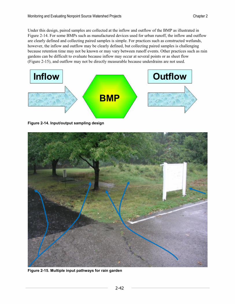
Monitoring and Evaluating Nonpoint Source Watershed Projects Chapter 2
2-42
Under this design, paired samples are collected at the inflow and outflow of the BMP as illustrated in Figure 2-14. For some BMPs such as manufactured devices used for urban runoff, the inflow and outflow are clearly defined and collecting paired samples is simple. For practices such as constructed wetlands, however, the inflow and outflow may be clearly defined, but collecting paired samples is challenging because retention time may not be known or may vary between runoff events. Other practices such as rain gardens can be difficult to evaluate because inflow may occur at several points or as sheet flow (Figure 2-15), and outflow may not be directly measurable because underdrains are not used.
Figure 2-14. Input/output sampling design
Figure 2-15. Multiple input pathways for rain garden

Monitoring and Evaluating Nonpoint Source Watershed Projects Chapter 2
2-43
Most sampling under this design will be storm-event based. Grab or automatic samples can be taken depending upon the specific practice evaluated, and either discrete or composite samples could be appropriate based upon specific study objectives. Flow measurements are essential to most BMP evaluations because performance usually varies with both flow rate and influent pollutant concentration.
With the exception of larger practices such as constructed wetlands and animal waste management systems, the possibility of having replicates and controls is an advantage of this design. No calibration period is required for inflow/outflow studies and measured pollutant reductions can be clearly attributed to the practice. A disadvantage of this design is the likelihood that results may not be widely transferable, but the relevance of this disadvantage will vary depending on the practice and study specifics. For example it may be possible to evaluate a manufactured urban stormwater device over a wide range of flow and influent concentrations at a single location, resulting in fairly widespread applicability.
Statistical methods commonly used for input-output studies are described in chapter 7 and include the paired t-test, nonparametric t-tests and the calculation of pollutant removal efficiencies. The effluent probability method is described in section 7.7.2.
2.4.2.10 Summary Table 2-4 matches monitoring objectives with appropriate monitoring designs. Reconnaissance is best for the assessment phase of a watershed project, but above/below monitoring can also be helpful in providing information about the isolated source or area. The paired, above/below-before/after, plot, and input/output designs are generally the best designs for evaluating the effectiveness of BMPs or watershed projects. All but reconnaissance, plot, and input/output monitoring can provide useful load estimation in support of TMDLs if flow and the relevant variables are monitored. Not surprisingly, the trend design is the best for trend detection.
Some monitoring designs can be used for more than one objective depending upon the location of monitoring stations, the schedule for BMP implementation, and the duration of the monitoring program. Both the single watershed and side-by-side watershed designs could be used for trend detection if monitoring is continued in a consistent manner over a longer than planned timeframe. It may be wise to actually plan for an extension of monitoring duration for trend detection under these two designs if they fail to yield results under a before/after monitoring design. Even above/below and paired designs could be extended for trend detection but the cost associated with continued monitoring over a longer timeframe would be very high; an alternative would be to consider extended monitoring for only the downstream (for above/below) or treatment (for paired) stations with some reduction in the set of monitoring variables or monitoring frequency to reduce costs. Any changes in monitoring frequency, however, would be contingent upon the ability to meet the requirement of consistent methods throughout a trend study.

Monitoring and Evaluating Nonpoint Source Watershed Projects Chapter 2
2-44
Table 2-4. Monitoring design as a function of objective
Design Short Description Variations
Objective
Prob
lem
Asse
ssm
ent
TMDL
Loa
ds
Tren
ds
BMP
or P
rojec
t Ef
fect
ivene
ss
Reconnaissance Multiple sites distributed across study area and monitored for a short duration (<12 months)
X
Plot Traditional research study design with varying treatments (BMPs) replicated in randomized block design
X
Paired Treatment and control watersheds monitored during a control and treatment period
Variation: nested-paired watershed—monitoring stations are in the same watershed
X X
Single watershed before/after
Single station at study area outlet monitored before and after BMP implementation
X X
Single-station long-term trend
Single station at study area outlet monitored before and after BMP implementation
Same as single watershed before/after without BMP implementation
X X
Above/below-(before/after)
Stations, with paired sampling, located upstream (up-gradient) and downstream (down-gradient) of BMP
Same as nested-paired-watershed design if sampled before and after BMP implementation
X X X
Side-by-side before/after
Same as single watershed since there are no calibrating paired samples
X X
Multiple Multiple watersheds monitored in two or more groups: treatment and control
X
Input/output Stations located at the input and output of an individual BMP
X
2.5 References ADEQ (Arizona Department of Environmental Quality). 2010. Oak Creek and Spring Creek Verde River
watershed total maximum daily loads for Escherichia coliform. Open File Report 10-01, Arizona Department of Environmental Quality. Accessed January 26, 2016.
Alberts, E.E., G. E. Schuman and R.E. Burwell. 1978. Seasonal runoff losses of nitrogen and phosphorus from Missouri Valley loess watersheds. Journal of Environmental Quality 7(2):203-208.
Algoazany, A.S., P.K. Kalita, G.F. Czapar, and J.K. Mitchell. 2007. Phosphorus transport through subsurface drainage and surface runoff from a flat watershed in east central Illinois, USA. Journal of Environmental Quality 36:681–693.

Monitoring and Evaluating Nonpoint Source Watershed Projects Chapter 2
2-45
Allmendinger, N.E., J.E. Pizzuto, G.E. Moglen, and M. Lewicki. 2007. A sediment budget for an urbanizing watershed, 1951-1996, Montgomery County, Maryland, U.S.A. Journal of the American Water Resources Association 43(6):1483-1498.
Bachman, L.J., D.E. Krantz, and J. Böhlke. 2002. Hydrogeologic Framework, Ground-Water Geochemistry, and Assessment of Nitrogen Yield from Base Flow in Two Agricultural Watersheds, Kent County, Maryland. EPA/600/R-02/008. U.S. Environmental Protection Agency, Office of Research and Development, Cincinnati, OH. Accessed January 26, 2016. http://water.usgs.gov/nrp/proj.bib/Publications/2002/bachman_krantz_etal_2002.pdf.
Baker, D.B. 1988. Sediment, Nutrient, and Pesticide Transport in Selected Lower Great Lakes Tributaries. EPA-905/4-88-001. Great Lakes National Program Office Report No. 1. Prepared for U.S. Environmental Protection Agency, Chicago, Illinois, by Heidelberg College, Water Quality Laboratory, Tiffin, OH.
Baker, D.B., K.A. Krieger, R.P. Richards, J.W. Kramer. 1985. Effects of Intensive Agricultural Land Use on Regional Water Quality in Northwestern Ohio. In Proceedings of Perspectives on Nonpoint Source Pollution, A National Conference, Kansas City, MO, May 19-22, 1985. EPA 440/5-85-001, U.S. Environmental Protection Agency, Office of Water Regulations and Standards, Washington, DC.
Bishop, P.L., W.D. Hively, J.R. Stedinger, M.R. Rafferty, J.L. Lojpersberger, and J.A. Bloomfield. 2005. Multivariate analysis of paired watershed data to evaluate agricultural best management practice effects on stream water phosphorus. Journal of Environmental Quality 34:1087–1101.
Blanton, J.O. 1975. Nearshore lake currents measured during upwelling and downwelling of the thermocline in Lake Ontario. Journal of Physical Oceanography 5:111–124.
Böhlke, J.K., M.E. O’Connell, and K.L. Prestegaard. 2007. Ground water stratification and delivery of nitrate to an incised stream under varying flow conditions. Journal of Environmental Quality 36:664-680.
Brakensiek, D.L., H.B. Osborn, and W.J. Rawls. 1979. Field Manual for Research in Agricultural Hydrology. Agriculture Handbook No. 224. U.S. Department of Agriculture, Science and Education Administration, Washington, DC.
CBF (Chesapeake Bay Foundation). n.d. Spring and Fall Salinity Levels. Chesapeake Bay Foundation. Annapolis, MD. Accessed January 26, 2016.
CBP (Chesapeake Bay Program). 1995. Chesapeake Bay: Introduction to an Ecosystem. Chesapeake Bay Program, Annapolis, MD.
CCRWQCB (Central Coast Regional Water Quality Control Board) and CPSU (California Polytechnic State University). 2003. Morro Bay National Monitoring Program: Nonpoint Source Pollution and Treatment Measure Evaluation for the Morro Bay Watershed 1992-2002 Final Report. Prepared for U.S. Environmental Protection Agency, by Central Coast Regional Water Quality Control Board and California Polytechnic State University – San Luis Obispo, CA. Accessed February 10, 2016. http://www.elkhornsloughctp.org/uploads/files/1149032089MorroBayEstuaryProgram.pdf.

Monitoring and Evaluating Nonpoint Source Watershed Projects Chapter 2
2-46
Chiles, J-P. and P. Delfiner. 1999. Geostatistics, Modeling Spatial Uncertainty. John Wiley, New York.
Clausen, J.C. 2007. Jordan Cove Watershed Project Final Report. University of Connecticut, College of Agriculture and Natural Resources, Department of Natural Resources Management and Engineering. Accessed January 8, 2016. http://jordancove.uconn.edu/jordan_cove/publications/final_report.pdf.
Coffey, S.W., J. Spooner, and M.D. Smolen. 1993. The Nonpoint Source Manager's Guide to Water Quality and Land Treatment Monitoring. North Carolina State University, Department of Biological and Agricultural Engineering, NCSU Water Quality Group, Raleigh, NC.
Cunningham, W.L., and C.W. Schalk, comps. 2011. Groundwater Technical Procedures of the U.S. Geological Survey. Techniques and Methods 1–A1. U.S. Geological Survey, Reston, VA. Accessed January 26, 2016. http://pubs.usgs.gov/tm/1a1/pdf/tm1-a1.pdf.
Davenport, T.E. 1984. Comprehensive monitoring and evaluation of the Blue Creek watershed. Lake and Reservoir Management 1(1):570-573.
DE CIB (Delaware Center for the Inland Bays). n.d. Wetlands and Waterways of the Inland Bays Watershed. Delaware Center for the Inland Bays, Rehoboth Beach, DE.
Dietz, M. 2006. Automated Introduction to the Paired Watershed Approach for Jordan Cove, Jordan Cove Urban Watershed Project. University of Connecticut, College of Agriculture and Natural Resources, Storrs, CT. Accessed January 26, 2016. http://jordancove.uconn.edu/jordan_cove/study_design.html.
Domagalski, J.L., S. Ator, R. Coupe, K .McCarthy, D. Lampe, M. Sandstrom and N. Baker. 2007. Comparative study of transport processes of nitrogen, phosphorus, and herbicides to streams in five agricultural basins, USA. Journal of Environmental Quality 37(3):1158-1169.
Donald, R., G. Southam, R. Foust, R. Rottach, and B.D. Burch. 1998. The Oak Creek Canyon Section 319(h) National Monitoring Project Final Report January, 1994-June, 1998. Prepared for U.S. Environmental Protection Agency, by Arizona Department of Environmental Quality. Northern Arizona University, Flagstaff, AZ.
Endale, D.M., D.S. Fisher, L.B. Owens, M.B. Jenkins, H.H. Schomberg, C.L. Tebes-Stevens, and J.V. Bonta. 2011. Runoff water quality during drought in a zero-order Georgia piedmont pasture: nitrogen and total organic carbon. Journal of Environmental Quality 40:969–979.
EPA (Environmental Protection Agency) Victoria. 2006. Hydrogeological Assessment (Groundwater Quality) Guidelines. Publication 668, ISBN 0 7306 7658 7. Environmental Protection Agency Victoria, Southbank, Victoria, Australia. Accessed January 26, 2016. http://www.epa.vic.gov.au/~/media/Publications/668.pdf.
Exner, M.E., H. Perea-Estrada, and R.F. Spalding. 2010. Long-term response of groundwater nitrate concentrations to management regulations in Nebraska’s Central Platte Valley. The Scientific World Journal 10:286-297.

Monitoring and Evaluating Nonpoint Source Watershed Projects Chapter 2
2-47
FACWI (Federal Advisory Committee on Water Information). 2013. A National Framework for Ground-Water Monitoring in the United States. The Subcommittee on Ground Water of the Federal Advisory Committee on Water Information. Accessed January 26, 2016. http://acwi.gov/sogw/ngwmn_framework_report_july2013.pdf.
Gaines, S. and S. Airame. 2010. Upwelling. Ocean Explorer. U.S. Department of Commerce, National Oceanic and Atmospheric Administration. Accessed January 26, 2016. http://oceanexplorer.noaa.gov/explorations/02quest/background/upwelling/upwelling.html.
Gaydos, J. 2009. Puget Sound Natural Resources Overview. In Puget Sound and a National Ocean Policy, The Ocean Foundation, Seattle, WA August 24, 2009. Accessed January 26, 2016. http://www.seadocsociety.org/files/pdfs/Gaydos-Presentation-Seattle-Ocean-Foundation-Mtg-Aug-09.pdf.
Gilliom, R.J., W.M. Alley, and M.E. Gurtz. 1995. Design of the National Water-Quality Assessment Program: Occurrence and Distribution of Water-Quality Conditions. Circular 1112. U.S. Geological Survey. Accessed January 26, 2016. http://pubs.usgs.gov/circ/circ1112/.
GLERL (Great Lakes Environmental Research Laboratory). 2011. Great Lakes Coastal Forecasting System. National Oceanic and Atmospheric Administration, Great Lakes Environmental Research Laboratory, Ann Arbor, MI. Accessed January 26, 2016. http://www.glerl.noaa.gov/res/glcfs/.
GLWWA (Grand Lake/Wabash Watershed Alliance). 2009. Grand Lake St. Marys/Wabash River Watershed Action Plan. Grand Lake/Wabash Watershed Alliance, Celina, OH. Accessed April 22, 2016. https://water.ohiodnr.gov/portals/soilwater/downloads/wap/Wabash.pdf.
Goodman, J., D. German, and J. Bischoff. 1996. Ground Water Monitoring – a Guide to Monitoring for Agricultural Nonpoint Source Pollution Projects. South Dakota Department of Environment and Natural Resources, Pierre, SD. Accessed April 22, 2016. https://archive.org/details/CAT10819301.
Haffner, G.D., M.L. Yallop, P.D.N. Hebert, and M. Griffiths. 1984. Ecological significance of upwelling events in Lake Ontario. Journal of Great Lakes Research 10(1):28-37.
Harmel, R.D., K.W. King, B.E. Haggard, D.G. Wren, and J.M. Sheridan. 2006. Practical guidance for discharge and water quality collection in small watersheds. Transactions of the American Society of Agricultural and Biological Engineers 49(4):937-948.
Hewlett, J.D. and L. Pienaar. 1973. Design and Analysis of the Catchment Experiment, In Proceedings of a Symposium on Use of Small Watersheds in Determining Effects of Forest Land Use on Water Quality, ed. E. H. White, University of Kentucky, Lexington, KY, May 22-23, 1973. Accessed January 26, 2016. http://coweeta.uga.edu/publications/hewlett_73_catachment.pdf.
Johnson, H.O., S.C. Gupta, A.V. Vecchia, and F. Zvomuya. 2009. Assessment of water quality trends in the Minnesota River using non-parametric and parametric methods. Journal of Environmental Quality 38:1018–1030.
Klatt, J.G., A.P. Mallarino, J.A. Downing, J.A. Kopaska and D.J. Wittry. 2003. Soil phosphorus, management practices, and their relationship to phosphorus delivery in the Iowa Clear Lake agricultural watershed. Journal of Environmental Quality 32(6):2140-2149.
Monitoring and Evaluating Nonpoint Source Watershed Projects Chapter 2
2-48
Lampert, W. 1989. The adaptive significance of diel vertical migration of zooplankton. Functional Ecology 3:21-27.
Lee, S-J., M.L. Serre, and G. Christakos. 2005. Bayesian maximum entropy mapping of arsenic using pH-arsenic empirical laws. ESE Research Notes 2(1):8-15. University of North Carolina, Department of Environmental Sciences and Engineering, Chapel Hill.
Lentz, R.D. and G. A. Lehrsch. 2010. Nutrients in runoff from a furrow-irrigated field after incorporating inorganic fertilizer or manure. Journal of Environmental Quality 39(4):1402-1415.
Lewis, J. 2006. Fixed and Mixed-Effects Models for Multi-Watershed Experiments. Pacific Southwest Research Station, U.S. Forest Service, Arcata, CA. Accessed March 24, 2016. http://www.fs.fed.us/psw/publications/4351/Lewis06.pdf.
MacDonald, L.H., A.W. Smart, and R.C. Wissmar. 1991. Monitoring Guidelines to Evaluate Effects of Forestry Activities on Streams in the Pacific Northwest and Alaska. EPA/910/9-91-001. U.S. Environmental Protection Agency, Region 10, Seattle, WA.
Meals, D.W. 2001. Lake Champlain Basin Agricultural Watersheds Section 319 National Monitoring Program Project, Final Project Report: May, 1994-September, 2000. Vermont Department of Environmental Conservation, Waterbury, VT.
Meals, D.W. and S.A. Dressing. 2008. Surface Water Flow Measurement for Water Quality Monitoring Projects. Tech Notes #9, September 2013. Prepared for U.S. Environmental Protection Agency, by Tetra Tech, Inc., Fairfax, VA. Accessed March 16, 2016. https://www.epa.gov/polluted-runoff-nonpoint-source-pollution/nonpoint-source-monitoring-technical-notes.
Meals, D.W., J. Spooner, S.A. Dressing, and J.B. Harcum. 2011. Statistical Analysis for Monotonic Trends, Tech Notes #6, September 2011. Prepared for U.S. Environmental Protection Agency, by Tetra Tech, Inc., Fairfax, VA. Accessed March 16, 2016. https://www.epa.gov/polluted-runoff-nonpoint-source-pollution/nonpoint-source-monitoring-technical-notes.
Montgomery, D.R. and J.M. Buffington. 1997. Channel-reach morphology in mountain drainage basins. Geological Society of America Bulletin 109: 596-611
MRGOMWNTF (Mississippi River/Gulf of Mexico Watershed Nutrient Task Force). 2008. Gulf Hypoxia Action Plan 2008. Mississippi River/Gulf of Mexico Watershed Nutrient Task Force. Accessed January 26, 2016. http://www.epa.gov/ms-htf/gulf-hypoxia-action-plan-2008.
NCSU (North Carolina State University) and Harbridge House. 1983. The Model Implementation Program: Lessons Learned From Agricultural Water Quality Projects. National Water Quality Evaluation Project at North Carolina State University and Harbridge House, Inc. Prepared for USDA and USEPA, Washington, DC.
Needelman, B.A., W.J. Gburek, G.W. Petersen, A.N. Sharpley, and P.J.A. Kleinman. 2004. Surface runoff along two agricultural hillslopes with contrasting soils. Soil Science Society of America Journal 68:914–923.
NOAA (National Oceanic and Atmospheric Administration). 1990. Estuaries of the United States: Vital Statistics of a National Resource Base. National Oceanic and Atmospheric Administration, Silver Spring, MD.

Monitoring and Evaluating Nonpoint Source Watershed Projects Chapter 2
2-49
OCWC (Oak Creek Watershed Council). 2012. Improvement Plan for the Oak Creek Watershed, Arizona. Prepared for Arizona Department of Environmental Quality, by Oak Creek Watershed Council, Sedona, AZ. Accessed April 22, 2016.
OEPA (Ohio Environmental Protection Agency). 2013. Statewide Biological and Water Quality Monitoring and Assessment. Ohio Environmental Protection Agency, Division of Surface Water, Columbus, OH. Accessed April 22, 2016. http://www.epa.state.oh.us/dsw/bioassess/ohstrat.aspx.
Ohrel, R.L. Jr. and K.M. Register. 2006. Volunteer Estuary Monitoring - a Methods Manual, Second Edition. The Ocean Conservancy, Washington, DC. Accessed January 27, 2016.
Plattner, S., D.M. Mason, G.A. Leshkevich, D.J. Schwab, and E.S. Rutherford. 2006. Classifying and forecasting coastal upwellings in Lake Michigan using satellite derived temperature images and buoy data. Journal of Great Lakes Research 32:63–76.
Poff, B. and A. Tecle. 2002. Bacteriological Water Quality Trend Analysis in Oak Creek Canyon, Arizona. In Ground Water/Surface Water Interactions, ed. J.F. Kenny, AWRA (American Water Resources Association) Specialty Summer Conference, Keystone, CO, July 1-3, 2002, pp. 431-436. Accessed April 22, 2016.
Rich. T. 2001. Results of Monitoring from 1989 through 1997 for the Statewide Ground Water Quality Monitoring Network. Open-File Report 89-UR. Prepared for South Dakota Department of Environmental and Natural Resources, by University of South Dakota, Akeley-Lawrence Science Center Science Center, Vermillion, SD. Accessed April 22, 2016. http://www.sdgs.usd.edu/pubs/pdf/UR-89%20-%20text.pdf.
Rosgen, D.L. and H.L. Silvey. 1996. Applied River Morphology. Wildland Hydrology Books, Fort Collins, CO.
Scalf, M.R., J.F. McNabb, W.J. Dunlap, R.L. Cosby, and J.S. Fryberger. 1981. Manual of Ground-Water Quality Sampling Procedures. U.S. Environmental Protection Agency, Office of Research and Development, Robert S. Kerr Environmental Research Laboratory, Ada, OK.
Schilling, K.E. 2002. Chemical transport from paired agricultural and restored prairie watersheds. Journal of Environmental Quality 31(4):1184-1193.
Schilling, K.E. and C.F. Wolter. 2001. Contribution of baseflow to nonpoint source pollution loads in an agricultural watershed. Ground Water 39(1):49-58.
SDDENR (South Dakota Department of Environment and Natural Resources). 2001. South Dakota’s Ground Water Quality Monitoring Network Project Completion Report: Section 319 Nonpoint Source Pollution Program. Prepared for U.S. Environmental Protection Agency, by South Dakota Department of Environment and Natural Resources, Division of Financial and Technical, Assistance, Geological Survey Program. Accessed April 22, 2016. http://denr.sd.gov/dfta/wp/Documents/GroundWaterMonitoring.pdf.
Sekely, A.C., D.J. Mulla, and D.W. Bauer. 2002. Streambank slumping and its contribution to the phosphorus and suspended sediment loads of the Blue Earth River, Minnesota. Journal of Soil and Water Conservation 57(5):243-250.

Monitoring and Evaluating Nonpoint Source Watershed Projects Chapter 2
2-50
Shirmohammadi, A., K.S. Yoon, and W.L. Magette. 1997. Water quality in mixed land-use watershed – Piedmont Region in Maryland. Transactions of the American Society of Agricultural Engineers 40(6):1563-1572.
Shirmohamadi, A. and H. Montas. 2004. Modeling and Monitoring the Hydrologic and Water Quality Response of the Mixed Land Use Basin FFY 03 Annual Report. University of Maryland, Department of Biological Resources Engineering, College Park, MD.
SIO (Scripps Institution of Oceanography). 2003. Waves, Nearshore Currents, and Tides. Coastal Morphology Group, Scripps Institution of Oceanography and the Kavli Institute. Accessed January 28, 2016. http://coastalchange.ucsd.edu/st3_basics/waves.html.
Slovinsky, P.A.. 2008. Coastal Circulation in the Vicinity of the Kennebunk River and Goochs Beach. Maine Geological Survey, Augusta, ME. Accessed April 22, 2016. http://www.maine.gov/dacf/mgs/explore/marine/sites/may08.pdf.
Sommer, T.R., W.C. Harrell, and T.J. Swift. 2008. Extreme hydrologic banding in a large-river floodplain, California, U.S.A., Hydrobiologia 598:409-415.
Spooner, J., L.A. Szpir, D.E. Line, D. Meals, G.L Grabow, D.L. Osmond and C. Smith. 2011. 2011 Summary Report: Section 319 National Monitoring Program Projects, National Nonpoint Source Watershed Project Studies. North Carolina State University, Biological and Agricultural Engineering Department, NCSU Water Quality Group, Raleigh, NC. Accessed March 15, 2016. http://www.bae.ncsu.edu/programs/extension/wqg/319monitoring/toc.html.
STAC (Scientific and Technical Advisory Committee). 2005. Understanding “Lag Times” Affecting the Improvement of Water Quality in the Chesapeake Bay. STAC Publ. 05–001. Chesapeake Bay Program, Edgewater, MD. Accessed January 27, 2016.
Stich, H. and W. Lampert. 1981. Predator evasion as an explanation of diurnal vertical migration by zooplankton. Nature 293(1):396-398.
Striffler, W.D. 1965. The selection of experimental watersheds and methods in disturbed forest areas. In IASH Symposium of Budapest 1965 - Representative and Experimental Basins, Publication No. 66, pp. 464-473, International Association of Hydrological Sciences. Accessed April 22, 2016. http://hydrologie.org/redbooks/a066/iahs_066_0464.pdf.
Stuntebeck, T.D., Komiskey, M.J., Owens, D.W., and Hall, D.W. 2008. Methods of Data Collection, Sample Processing, and Data Analysis for Edge-of-Field, Streamgaging, Subsurface-Tile, and Meteorological Stations at Discovery Farms and Pioneer Farm in Wisconsin, 2001–7. Open-File Report 2008–1015. U.S. Geological Survey, Reston, VA. Accessed April 22, 2016. http://pubs.usgs.gov/of/2008/1015/pdf/ofr2008-1015.pdf.
Suppnick, J. 1999. Water Chemistry Trend Monitoring in Sycamore Creek and Haines Drain, Ingham County, Michigan 1990-1997. Staff report MI/DEQ/SWQD-99-085. Michigan Department of Environmental Quality, Surface Water Quality Division. Accessed April 29, 2016. https://www.epa.gov/polluted-runoff-nonpoint-source-pollution/monitoring-and-evaluating-nonpoint-source-watershed.
Monitoring and Evaluating Nonpoint Source Watershed Projects Chapter 2
2-51
Taylor, C.B. and H.B. Stewart. 1959. Summer upwelling along the east coast of Florida. Journal of Geophysical Research 64(1): 33-40.
Taylor, C.J. and W.M. Alley. 2001. Ground-Water-Level Monitoring and the Importance of Long-Term Water-Level Data. Circular 1217, U.S. Geological Survey, Denver. CO. Accessed January 28, 2016. http://pubs.usgs.gov/circ/circ1217/pdf/circular1217.pdf.
Tetra Tech. n.d. Section 319 National Monitoring Program Projects Lessons Learned. Prepared for U.S. Environmental Protection Agency, by Tetra Tech, Inc., Fairfax, VA. Accessed April 29, 2016. https://www.epa.gov/polluted-runoff-nonpoint-source-pollution/monitoring-and-evaluating-nonpoint-source-watershed.
Tiner, R.W. 2002. In Search of Swampland – A Wetland Sourcebook and Field Guide. Rutgers University Press, New Brunswick.
USDA-NRCS (U.S. Department of Agriculture-Natural Resources Conservation Service). 2003. National Water Quality Handbook. 450–VI–NWQH. U.S. Department of Agriculture, Natural Resources Conservation Service, Washington, DC. Accessed January 29, 2016. http://www.nrcs.usda.gov/Internet/FSE_DOCUMENTS/stelprdb1044775.pdf.
USEPA (U.S. Environmental Protection Agency). 1983. Results of the Nationwide Urban Runoff Program: Volume 1 - Final Report. U.S. Environmental Protection Agency, Office of Water, Washington, DC. Accessed January 28, 2016. http://www.epa.gov/npdes/pubs/sw_nurp_vol_1_finalreport.pdf.
USEPA (U.S. Environmental Protection Agency). 1990. The Lake and Reservoir Restoration Guidance Manual. EPA-440/4-90-006. U.S. Environmental Protection Agency, Office of Water, Washington, DC.
USEPA (U.S. Environmental Protection Agency). 1993a. Evaluation of the Experimental Rural Clean Water Program. EPA-841-R-93-005. U.S. Environmental Protection Agency, Office of Wetlands, Oceans, and Watersheds, Washington, DC.
USEPA (U.S. Environmental Protection Agency). 1993b. Paired Watershed Study Design. EPA 841-F-93-009. U.S. Environmental Protection Agency, Washington, DC.
USEPA (U.S. Environmental Protection Agency). 1997. Monitoring Guidance for Determining the Effectiveness of Nonpoint Source Controls. EPA 841-B-96-004. U.S. Environmental Protection Agency, Office of Water, Washington, DC. Accessed March 16, 2016. https://www.epa.gov/polluted-runoff-nonpoint-source-pollution/monitoring-guidance-determining-effectiveness-nonpoint.
USEPA (U.S. Environmental Protection Agency). 1998. Nearshore Waters and Your Coastal Watershed. EPA 842-F-98-007. U.S. Environmental Protection Agency, Washington, DC. Accessed January 28, 2016.
USEPA (U.S. Environmental Protection Agency). 2001. EPA Requirements for Quality Assurance Project Plans, EPA QA/R-5. EPA 240/B-01/003. U.S. Environmental Protection Agency, Office of Environmental Information. Washington, DC.
Monitoring and Evaluating Nonpoint Source Watershed Projects Chapter 2
2-52
USEPA (U.S. Environmental Protection Agency). 2002a. Methods for Evaluating Wetland Condition: #16 Vegetation-Based Indicators of Wetland Nutrient Enrichment. EPA-822-R-02-024. U.S. Environmental Protection Agency, Office of Water, Washington, DC. Accessed January 15, 2016. http://www.epa.gov/sites/production/files/documents/wetlands_16indicators.pdf.
USEPA (U.S. Environmental Protection Agency). 2002b. Methods for Evaluating Wetland Condition: Study Design for Monitoring Wetlands. EPA-822-R-02-015.U.S. Environmental Protection Agency, Office of Water, Washington, DC.
USEPA (U.S. Environmental Protection Agency). 2003a. Elements of a State Water Monitoring and Assessment Program. EPA 841-B-03-003. U.S. Environmental Protection Agency, Office of Water, Office of Wetlands, Oceans and Watersheds, Assessment and Watershed Protection Division, Washington, DC. Accessed January 28, 2016.
USEPA (U.S. Environmental Protection Agency). 2003b. Guidance for 2004 Assessment, Listing and Reporting Requirements Pursuant to Sections 303(d) and 305(b) of the Clean Water Act, July 21, 2003. United States Environmental Protection Agency, Office of Water, Office of Wetlands, Oceans, and Watersheds, Assessment and Watershed Protection Division, Watershed Branch, Washington, DC. Accessed January 28, 2016.
USEPA (U.S. Environmental Protection Agency). 2004. Review of Rapid Assessment Methods for Assessing Wetland Condition. EPA/620/R-04/009. U.S. Environmental Protection Agency, National Health and Environmental Effects Laboratory, Corvallis, OR.
USEPA (U.S. Environmental Protection Agency). 2006a. Application of Elements of a State Water Monitoring and Assessment Program For Wetlands. U.S. Environmental Protection Agency, Office of Water, Office of Wetlands, Oceans, and Watersheds, Wetlands Division, Washington, DC.
USEPA (U.S. Environmental Protection Agency). 2006b. Guidelines for the Award of Monitoring Initiative Funds under Section 106 Grants to States, Interstate Agencies, and Tribes. U.S. Environmental Protection Agency, Washington, DC. Federal Register, March 29, 2006, 71:15718-15724. Accessed January 28, 2016. https://federalregister.gov/a/E6-4585.
USEPA (U.S. Environmental Protection Agency). 2008a. Amendment to the Guidelines for the Award ofMonitoring Initiative Funds under Section 106 Grants to States, Interstate Agencies, and Tribes. U.S. Environmental Protection Agency, Washington, DC. Federal Register, July 17, 2008, 73:41069-41076. Accessed January 28, 2016. https://federalregister.gov/a/E8-16385.
USEPA (U.S. Environmental Protection Agency). 2008b. Handbook for Developing Watershed Plans to Restore and Protect Our Waters. EPA 841-B-08-002. U.S. Environmental Protection Agency, Office of Water, Washington, DC. Accessed February 10, 2016. http://www.epa.gov/polluted-runoff-nonpoint-source-pollution/handbook-developing-watershed-plans-restore-and-protect.
USEPA (U.S. Environmental Protection Agency). 2011. Aquatic Resource Monitoring - Frequently Asked Questions - Survey Sampling. U.S. Environmental Protection Agency, Office of Research and Development, National Health and Environmental Effects Research Laboratory, Western Ecology Division, Corvallis, OR. Accessed January 28, 2016. http://archive.epa.gov/nheerl/arm/web/html/designfaqs.html.
Monitoring and Evaluating Nonpoint Source Watershed Projects Chapter 2
2-53
USEPA (U.S. Environmental Protection Agency). 2012a. EPA Program Guidance. U.S. Environmental Protection Agency, Washington, DC. Accessed January 28, 2016. http://water.epa.gov/lawsregs/lawsguidance/cwa/tmdl/guidance.cfm#program.
USEPA (U.S. Environmental Protection Agency). 2012b. Starting Out in Volunteer Monitoring. EPA 941-F002-004. U.S. Environmental Protection Agency, Office of Water, Washington, DC. Accessed January 28, 2016.
Wagner, R.J., R.W. Boulger, Jr., C.J. Oblinger, and B.A. Smith. 2006. Guidelines and Standard Procedures for Continuous Water-Quality Monitors—Station Operation, Record Computation, and Data Reporting. Techniques and Methods 1–D3. U.S. Geological Survey, Reston, VA. Accessed January 28, 2016. http://pubs.usgs.gov/tm/2006/tm1D3/.
WAL (Wisconsin Association of Lakes). 2009. Lake Types: How Does Water Get into Your Lake? Wisconsin Association of Lakes, Madison, WI. Accessed January 28, 2016. http://www.wisconsinlakes.org/index.php/the-science-of-lakes/21-lake-types.
Welch, E.B. and G.D. Cooke. 1999. Effectiveness and longevity of phosphorus inactivation with alum. Journal of Lake and Reservoir Management 15:5-27.
Wetzel, R.G. 1975. Limnology. W.B. Saunders Company, Philadelphia, PA.
Wilde, F.D. 2005. Preparations for Water Sampling. Book 9, Chapter A1 in Techniques of Water-Resources Investigations. U.S. Geological Survey, Reston, VA. Accessed January 28, 2016. http://pubs.water.usgs.gov/twri9A1/.
Wilde, F.D., ed. 2006. Collection of Water Samples (Version 2.0). Book 9, Chapter A4 in Techniques of Water-Resources Investigations. U.S. Geological Survey, Reston, VA. Accessed January 28, 2016. http://pubs.water.usgs.gov/twri9A4/.
Wilson, M.L., C.J. Rosen, and J.F. Moncrief. 2010. Effects of polymer-coated urea on nitrate leaching and nitrogen uptake by potato. Journal of Environmental Quality 39: 2: 492-499.
Winter, T.C., J.W. Harvey, O.L. Franke, and W.M. Alley. 1998. Ground Water and Surface Water a Single Resource. Circular 1139. U.S. Geological Survey, Denver. Accessed January 28, 2016. http://pubs.usgs.gov/circ/circ1139/index.html.
Zaret, T.M. and J.S. Suffern. 1976. Vertical migration in zooplankton as a predator avoidance mechanism. Limnology and Oceanography 21(6):804-813.

Monitoring and Evaluating Nonpoint Source Watershed Projects Chapter 2
2 -54
This page intentionally left blank.