Embed Size (px)
Citation preview

Money Stock Control
ALBERT E. BURGER*
The Federal Reserve stated in 1960, when it began publishing aseparate and distinct money stock series, that:
The amount of money in existence and changes in this amount influ-ence the course of economic developments ....
The Federal Reserve Syste,n has priznary responsibility for regulatingthe total volume of money available to meet the pubhc s demands..
Over the next 10 years a major controversy developed overwhether the Federal Reserve recognized or placed enough emphasison its responsibility for controlling the growth of the money stock.The related question of which operating strategy to follow in con-trolling the money stock was pushed to the background.
Economists can argue at great lengths over the extent to which theFederal Reserve tried to control money in the past. However, onething is clear: since early 1970, the Federal Open Market Committee(FOMC) has moved in several stages to a position of placing moreemphasis on controlling the money stock, relative to other objec-tives, than had previously been the case. Along with this move, therehave been increased scrutiny of the current operating strategy and ananalysis of the problems involved in controlling growth rates ofmonetary aggregates.
In the spring of 1969 Chairman Martin appointed a subcommitteewithin the Federal Reserve under the leadership of GovernorSherman Maisel to study means of improving open market opera-tions. The Maisel Committee focused on the problem that, if moneymarket conditions are the primary target of open market operations,then the FOMC has no clear and definite way of giving instructionsto the Manager of the System Open Market Account. The Com-mittee’s primary concern was more with improving the performance
*Economist, Federal Reserve Bank of St. LouisThe author wishes to express his appreciation to Robert Rasche and Anatol Balbach for
their many comments on this subject. The author also acknowledges the valuable technical,programming, and editorial assistance of Marie Wahlig and Mary Thoenen. The proceduresand conclusions are the responsibility of the author.
I"A New Measure of the Money Supply," Federal Reserve Bultetin (October 1960), p.1102.
33

34 CONTROLLING MONETARY AGGREGATES II
of open market operations to accomplish the FOMC’s goals, ratherthan with the technical aspects of open market operations,x One ofthese studies, "Short-Run Targets for Open Market Operations,"prepared by Richard G. Davis, dealt primarily with the short-runoperating procedures. The series of studies prepared for the MaiselCommittee was published by the Federal Reserve in 1971.~ Sincethat time there has been considerable additional research and dis-cussion within the Federal Reserve System on the problem ofcontrolling monetary aggregates.
In this paper, the control of one monetary aggregate, the moneystock, is considered. It is assumed that the Federal Open MarketCommittee has chosen a growth path for the money stock it expectsto be consistent with its policy objectives for output, employment,and prices. All the problems relating to how the growth path waschosen are ignored. The control problem is to use open marketoperations to achieve that growth path for money. This involvespredicting the effects of open market operations on the moneystock. Because of information lags and random weekly fluctuationsin money, the Federal Reserve does not aim open market operationsdirectly at the money stock, but picks an operating target inter-mediate between open market operations and the money stock. Thetwo main candidates for this operating target have been the Federalfunds rate and some reserve aggregate.
A general reserve aggregate-multiplier approach is used to derive acontrol procedure the FOMC could use to achieve a desired growthpath for money. The connecting link between the reserve aggregate,be it total reserves, nonborrowed reserves, the monetary base, orsome variant of these, and the money stock is called a multiplier. Themoney stock control procedure involves predicting the effect on themoney stock of setting the reserve aggregate at a given value. Theform of the control procedure developed in this article is quitegeneral and could also be applied to the problem of controlling otheraggregates such as M2 or bank credit.
This is not the only approach that could be taken to the problemof controlling the money stock. Other economists within the FederalReserve have attacked the problem from a different approach. The
2Andrew F. Brimmer, "The Political Economy of Money: Evolution and Impact ofMonetarism in the Federal Reserve System," American Economic Review (May 1972), p.350.
30pen Market Policies and Operating Procedures -- Staff Studies (Washington, D.C.:Board of Governors of the Federal Reserve System, 1971).

MONEY STOCK CONTROL BURGER 35
method developed in this paper, however, provides a frameworkwithin which several aspects of money stock control can be analyzed,and perhaps, most importantly, provides a minimum standard ofcontrol against which other proposed methods can be compared.4
The determination of the money stock is summarized in amultiplier-base expression of the following form:5
M1 = mB
where"M1’’ is the money stock (de~nand deposits plus currency heldby the nonbank public), "B" is the net source base, and "m" is themoney multiplier. The net source base (B) can be controlled byFederal Reserve open market operations. Sometimes this baseconcept is referred to as the nonborrowed base to denote that mem-ber bank borrowings are excluded. The net source base is taken asthe control variable in the procedure set forth in this article. In itsday-to-day operations this would be the variable toward which theDesk would primarily direct its open market operations.6 It isassumed that, using open market operations, the Desk can set the netsource base at the value it desires for a monthly period.
On a daily basis, the Federal Reserve has information on the valueof the previous day’s net source base. This information comes fromtotaling the sources of the base, as shown in Table I. Special care
james Pierce and Thomas Thomson have also studied, the probl(m, with their monthlymoney market model using the Federal funds rate as the control variable. Richard Davis hasused a reduced form relationship that takes the demand deposit component of the moneystock as the variable to be explained. His reduced form equation includes nonborrowedreserves (or alternatively the Federal funds rate), business sales, Government deposits and avariable to capture the effects of Regulation Q. See James L. Pierce and Thomas D.Thomson, "Some Issues in Controlling the Stock of Money," pp. 115-136 in this volume.
5Tbe specific procedure presented in this paper is designed within the framework of anon-linear money supply hypothesis developed by Karl Brunner and Allan Meltzer:
m = l+k(r-b) (l+t+d)+k
where k, t, and d, respectively, are the ratios of currency held by the public, time deposits,and U.S. Government demand deposits at commercial banks to the demand deposit com-ponent of the money stock.
The variables r and b, respectively, are the ratios of bank reserves and member bankborrowings to commercial bank deposit liabilities (excluding interbank deposits). See KarlBrunner and Allan H. Meltzer, "Liquidity Traps for Money, Bank Credit, and InterestRates," Journal of Political Economy (January]February 1968), pp. 1-37, and Albert E.Burger, The Money Supply Process {Belmont, California: Wadsworth, 1971).
6The Manager of the System Open Market Account may be referred to as the "AccountManager" or the "Desk," meaning the Trading Desk of the New York Federal Reserve Bank.

SOURCES AND USES OF THE NET SOURCE BASE,THE SOURCE BASE,
AND THE MONETARY BASE, JANUARY 1970~(mialions of dollars)
Sources
Federal Reserve holdings ofGovernment securities $56,346
Federal Reserve floa’~ 3,442Gold stock plus special
drawing rightsTreasury currency outstanding 6,856Other Federal Reserve assetsLess:
Treasury cash holdings 655Treasury deposits at Fed-
eral Reserve BanksForeign deposits at Fed-
eral Reserve Banks 170:Other deposits at Federa! Reserve plus
Federal Reserve liabilities and capital 2,686Equals:
N ET SO U RCE- BASE $75,337Plus:
Federa! Reserve discountsand advances 965
Equals:Source base $76,302
Plus:Reserve adjustment 3,172
Equals:Monetary base $79,474
*Data are not seasonally adjusted.
Member bank deposits atFederal Reserve Banks lessdiscounts and advances $22,615
Currency held by banks 6,622Currency held by the public 46,100
Equals:NET SOURCE BASE $75,337
P~us:Federal Reserve discounts
and advances 955Equals:
Source base $76,302P~us:
Reserve adjustment 3,172Equals:
Monetary base $79,474

MONEYSTOCKCONTROL BURGER 37
should be taken to distinguish between the sources and uses of thebase. To get its bearings on the base, the Desk does not have toestimate excess reserves and currency. This would be the case only ifthe Manager of the System Open Market Account had to rely solelyon information about the uses of the base. By collecting the data onthe sources of the base, which come from the books of the FederalReserve and the Treasury, a closer estimate can be obtained on ashort-run basis.
The money multiplier (m) is the connecting link between the netsource base and money stock. Changes in the multiplier reflect port-folio decisions by banks and the public, Treasury actions, andFederal Reserve policy actions such as changes in reserve require-ments and the discount rate. The multiplier is not constant. There-fore, under this proposed procedure, the Federal Reserve mustestimate the multiplier to determine how much base to supply toachieve a desired path for the money stock.
Forecasting the Money Multiplier
The procedure used to forecast the money multiplier was set up torequire a minimum amount of forecasted information. If some of theinputs into the multiplier forecasting process must be predicted,additional sources of error are added. The procedure used in thispaper takes as inputs only those variables that the Federal Reservecould be assumed to know without error. In essence, this is a verymechanical method that does not attempt to incorporate any infor-mation the Federal Reserve might have about expected movementsof key factors such as Treasury deposits in the forecast month.Therefore, the results of the procedure should not be viewed as anindication of the best control the Federal Reserve could attain.Instead, they provide a standard against which other procedurescould be evaluated. Any alternative procedure should be able toperform at least as well as this simple, mechanical method.
A not seasonally adjusted M1 multiplier is forecast. The regressionequation used to forecast the money multiplier uses the lagged3-month moving average of past values of the multiplier (mr-1 + mr_2+ m 3)/3, the lagged percentage change in the market yield ont-3-month Treasury bills [TBt.1 - TBt.2]/TBt.2, and seasonal dummyvariables.
The coefficients used to forecast each month’s multiplier areestimated by least squares using the previous 36 months’ observa-tions. Each month the coefficients are re-estimated by adding the

38 CONTROLMNG MONETARY AGGREGATESII
most recent month and dropping the first month of the previous 36observations. In making the forecasts 0ut_1 term is added, whereis the lagged value of ~he error in the estimate of the money mufti-plier and p is the correlation coefficient for consecutive error termsin the equation during the sample period.7 This procedure is anextension of the procedure used in an article co-authored with LionelKNish and Christopher Babb.8 ’The major modification is to removethe reserve adjustment magnitude and include the lagged percentagechange in the Treasury bill rate.
Variables that may have an important influence on the value ofthe multiplier are excluded by the criterion used to restrict the set ofeligible regressors. The influences of these variables are impounded inthe error term, and the question may arise as to whether their exclu-sion is likely to seriously bias the estimated coefficients of theincluded variables. One important excluded effect is contempor-aneous changes in interest rates. The method for forecasting themoney multiplier takes into account only the lagged effects ofchanges in interest rates on the multiplier. Open market operations inthe current month influence interest rates in the current month, andthis impact effect on the multiplier is not included in the forecastingprocedure. If the impact or current month interest rate effects ofopen market operations on the multiplier are substantial, then animprovement in forecasting might result from including projectionsof interest rates in the forecasted month. However, since theseimpact interest rate effects on the money multiplier appear to besmall, and projecting interest rates involves an unknown error, onlylagged interest rate effects were included.9
7Rho is estimated as 1- 2~-~, where DW is the Durbin-Watson statistic. The absolute meanvalue of p over the 1964-71 period was .47, no value of p exceeds .75 and only 27 of the 96values of p exceed .60.
8Albert E. Burger, Lionel Kalish III and Christopher T. Babb, "Money Stock Control andIts Implications for Monetary Policy," Federal Reserve Bank of St. Louis Review (October1971), pp. 6-22, available as Reprint :pp 72.
9Robert H. Rasche has surveyed the empirical evidence on interest sensitivity of themoney multiplier, beginning with studies by Teigen, DeLeeuw, Goldfeld and Kane, andBrunner and Meltzer and ending with recent evidence provided by the Federal Reserve-M.I.T.-Pennsylvania econometric model and a financial market model by Thomson andPierce. Rasche concludes that the accumulated empirical evidence indicates that the interestelasticity of the money supply relationship during the sample period of these studies appearsto be extremely low, with the impact elasticity in the range of 0.10 to 0.15. Hence theshort-run feedback effects tlu’ough interest rate changes wifich would be generated by policychanges in reserve aggregates m’e weak and should cause little difficulty for controlling themoney stock through control of a reserve aggregate. See Robert H. Rasche, "A Review ofEmpirical Studies of the Money Supply Mechanism," Federal Reserve Bank of St. LouisReview (July 1972), pp. 11-19.

MONEY STOCK CONTROL BURGER 39
Two other effects are changes in Treasury deposits in the currentmonth and reserve requirement changes. Changes in Treasurybalances are primarily determined by current tax receipts andexpenditures of the Government and are probably uncorrelated withthe regressors used to estimate the multiplier. Reserve requirementchanges are infrequent and it is unlikely there is significant correla-tion between them and the regressors. One excluded variable thatcould bias the coefficients is Regulation Q ceiling rates. There couldbe a sizeable correlation between a variable capturing the effect ofRegulation Q and the lagged 3-month average of the multiplier whenthe ceiling rate is effective. The basic problem is the appropriatemeans of specifying the effect of Regulation Q. A varied selection ofcandidates was tried in the research for this paper, but at present nosatisfactory proxy has been developed.
Simulating the Control Procedure
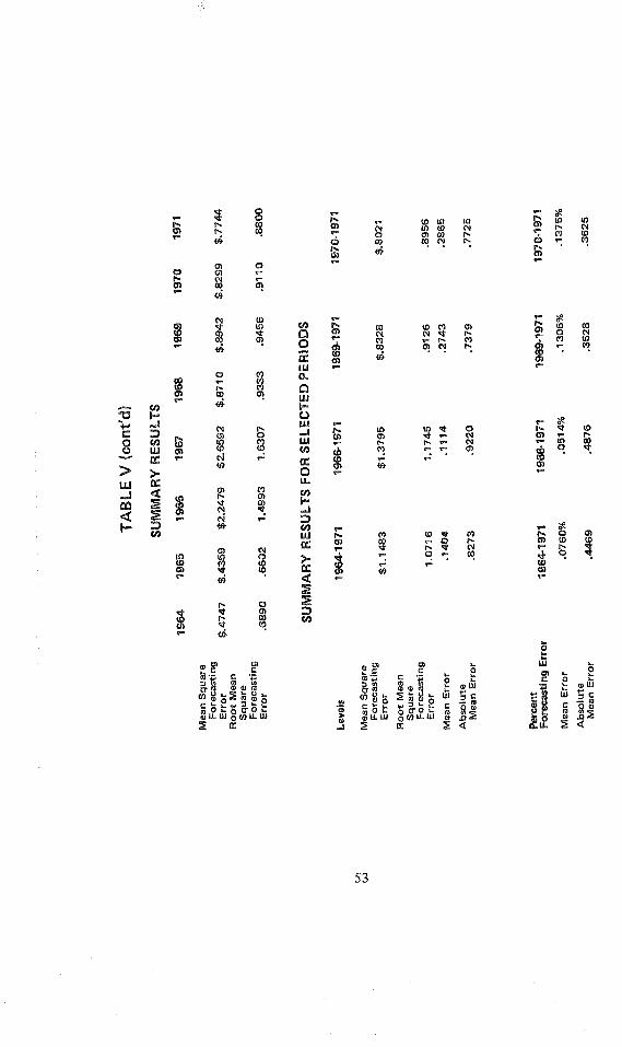
The results of simulating this procedure over the 8-year period1964-71 are presented in Table V at the end of the article. Since noforecasting errors are involved in the independent variables, theresults of these simulations indicate how well the procedure wouldhave worked over the 1964-71 period. When comparing these resultswith results from other methods, care must be taken to determinewhether any of the variables used in the alternative procedures mustbe forecast. For example, an alternative which stresses the demandfor money might include income or some proxy such as businesssales in the forecasting period as an independent variable. If simula-tions of this type of procedure use actual values for income or itsproxy, the errors will be biased downward to the extent that fore-casting errors for income have not been taken into consideration.
The results in Table V were generated in the following manner:the forecasted not seasonally adjusted money multiplier was multi-plied by the actual not seasonally adjusted net source base to obtainnot seasonally adjusted money (NSAM).1° Then NSAM was multi-plied by the implicit seasonal factor for that month to obtain the
10In the previous article, Burger, Kalish, Babb, "Money Stock Control and Its Implica-tions for Monetary Policy," a desired growth path for M1 was chosen. Then, the moneymultiplier was forecast and the net source base was set to achieve the desired M1. Thecontrolled M1 was computed by multiplying the actual (historical) multiplier by the con-trolled value ~of the net source base. Errors were computed by comparing controlled anddesired M1. In this article the net source base is set at its actual (historical) values. Themoney stock the FOMC would have expected, given the forecasts of the money multiplier,is computed by multiplying the forecasted multiplier by the actual net source base. Errorsare computed by comparing thig projected value of M1 with actual (historical) M1.

4O CONTROLLING MONETARY AGGREGATES II
seasonally adjusted money stock. The regression equation used toforecast the multiplier was estimated using not seasonally adjusteddata, and the implicit seasonal factor was computed by dividingactual seasonally adjusted money by actual not seasonally adjustedmoney. There is a different regression equation used to obtain thecoefficients to forecast each month, hence, 96 regression equations.Therefore, the results of these equations are not reported. The resultsfor January 1970 are reported in Table II to illustrate the procedureand to aid in reproducing the results.11
The example in Table II may be analyzed in the following manner.Using the forecasting procedure, the Federal Reserve would haveforecast the January 1970 money multiplier to be 2.80095. Hence, ifthey had set the NSA net source base at $75.337 billion, then theywould have expected seasonally adjusted money to equal $205.126billion. The NSA net source base was $75.337 (see Table I) andactual money was $205.500 billion. Therefore, using this procedurewould have resulted in underestimating the effect of their actions by$374 million.
There are several ways of evaluating the simulation resultsreported in Table V. One approach is to look at the monthly errorsand compute the mean square forecasting error, root mean-squareforecasting error, and mean and absolute mean forecasting errors. Asshown at the end of Table V, the root mean square monthly fore-casting error over the whole period is $1.07 billion, the absolutemean percent forecasting error is 0.45 percent.12 The mean fore-casting error is $140 million and the mean percent forecasting erroris 0.1 percent, which indicate that the procedure, on average, doesnot substantially over-or underestimate the money stock associatedwith a set value of the net source base.
A sharp distinction must be made between forecasting money onemonth in advance and controlling money. The evaluation of theperformance of a money stock control procedure should not bebased solely on monthly errors. For example, a half a percent errorin one month, converted to an annual rate becomes a 6 percent error.
llThe mean value of the coefficient on the lagged B-month moving average of themultiplier is .8867, and is significant in all regressions as indicated by a range of t-values ofapproximately 5 to 15. The coefficient on the lagged percent change in the Treasury billrote is generally insignificant in the first 4½ years of the sample period and generallysignificant in regressions used to estimate coefficients for forecasting the last 3½ years, thisfinal period having a mean value of. 1128.
12The percent forecasting error for each month is forecasted minus actual money dividedby actual multiplied by 100.

MONEY STOCK CONTROL BURGER 41
TABLE |1
EXAMPLE OF THE PROCEDURE USED TOFORECAST THE MONEY STOCK
Period: January 1970
Regression equation based on 36 months ended December 1969:1
m = 0.79566 + 0.72002 19lAY + 0.11888 TB(5.06) (2.70)
+ ,00932 DI R2= ,87SE = .01170
MAY = lagged 3-month moving average of the money multiplierTB = lagged percent change in Treasury bill rateDi = seasonal dummy for January
Data used to forecast January 1970 multiplier:
MAY = 2.77206 = average of October-December, 1969TB = 0.07873p = 0.4836put_1 = --0.00933
Forecast of the multiplier:
2.80095 = 0.79566 + (0.72002) (2.77206) + (0.11888)(0.07873) + 0.00932 - 0.00933
Forecast of seasonally adjusted money:
Actual net source base (NSA) for January 1970 = $76,337Forecasted not seasonally adjusted money = ($75.337) (2,80095)
= $211.015
Seasonal factor- Actual SA Money 205,500 0.97209Actual NSA Money 211
Forecasted seasonally adjusted money = ($211o015) (0,97209)= $205.126
Forecasted minus actual seasonally adjusted money = $205.126 -- $205.500=
1The equation was estimated by least squares using not seasonally adjusted data.Numbers in parentheses are t-values.
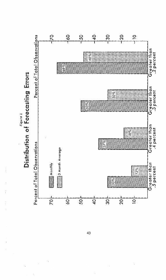
This does not necessarily imply that using this method would resultin that magnitude of error over a relevant control period. Errors donot tend to accumulate, and positive errors are offset by negativeones. Computing consecutive 3-month moving averages of forecastedand actual money over the 1964-71 period results in a mean percenterror of .07 percent and an absolute mean percent error of .31

42 CONTROLLING MONETARY AGGREGATES I[
percent. A comparison of errors for 3-month moving averages withmonthly errors is presented in Figure I. Only 12 percent of the totalerrors for 3-month moving averages are greater in absolute value than0.5 percent, compared to 28 percent of the monthly errors. Theseresults also support the conjecture that over a relevant control periodthis simple control procedure would result in relatively .close controlover the money stock. In other words, if the desired level of themoney stock can be expressed as an average for a 3-month period theprocedure should permit its achievement with only small errors.
Another means of analyzing the effectiveness of the controlprocedure is to compare the expected growth rates of the moneystock resulting from simulating the control procedure with actualgrowth rates of the money stock. The simulated monthly values ofthe money stock are what the FOMC would have expected fromsetting the net source base at its historical values if it had been usingthis procedure to forecast the money multiplier.
In this way, an analysis can be made of the effectiveness of thecontrol procedure at times when there were marked reversals in thegrowth rate of the money stock. During the period 1964-71 therewere at least 6 marked changes in the growth rate of the moneystock. Table III presents a comparison of actual growth rates ofmoney and the growth rates that the FOMC would have expected ifit had been using the control procedure over these periods.
For example, beginning in mid-1966 the growth rate of moneyslowed markedly. By setting the net source base at its historicalvalues, the FOMC would have expected, given the forecasts of themoney multiplier, that the money stock would have grown at a 1.1percent annual rate from the average of 3 months ended May 1966to the average of 3 months ended December 1966. The actual growthrate of the money stock over this same period was 0.2 percent. Inearly 1967 the FOMC moved to a much more expansionary policy.Simulating the control procedure results in an expected growth rateof the money stock of 7.1 percent from the average of 3 monthsended December 1966 to the average of 3 months ended January1969. The actual growth rate of money associated with setting thenet source base at its historical values was 7.2 percent over thisperiod.
Dis
tribu
tion
Per
cen~
of T
otal
Obs
erva
tions
Fig
ure
~
Fore
cast
ing
~:rr
ors
Pe
rce
n’t
of
To~a
~ O
bse
rva
tion
s
7O
6O 5O 4O 3O
2O 10
~ M
on
thly
~3
Mo
n~
’h A
ve
rag
e
Gre
ate
r th
an
.5 p
erce
n’~
- 70
- 60
- 50
- 40
- 30
- 20
- 10

44 CONTROLLING MONETARY AGGREGATES II
Federal Reserve Induced Impediments to Money Stock Control
The 1964-71 period presented an especially difficult period formoney stock control. A significant part of this difficulty was intro-duced by Federal Reserve actions. During this 8-year period therewere several major reversals in the direction of the influence ofFederal Reserve policy actions on the money stock.13 In addition,reserve requirements were changed 7 times and lagged reserverequirements were introduced in this period. The Federal Reservealso permitted Regulation Q ceiling rates to frequently restrain banksfrom responding in a competitive manner to changes in marketrates.14
The money stock control procedure developed in this article is notdesigned to capture the initial effects of these actions by the FederalReserve. Because a lagged 3-month moving average of the multiplieris used, a sharp reversal of policy may cause a change in the moneymultiplier that is not immediately captured by the procedure used toforecast the multiplier. For example, at times of sharp reversals inthe growth rate of the money stock relatively larger forecastingerrors occur. After mid-1966 the forecasting procedure substantiallyoverestimates the multiplier, and the opposite occurs in early 1967.Also, a similar tendency seems to have been in effect in 1971 aserrors tended to be negative in the first half of the year and positivein the second half. The exact size and direction of this effect dependsupon a number of factors; however, given the characteristics of theprocedure used to forecast the multiplier, it does seem likely that asubstantial change in the thrust of open market policy on the moneystock will introduce additional problems for accurately predictingthe initial influence of open market actions on the money stock.
The results shown in Table III and discussed at the end of theprevious section, however, show that the FOMC could quite accu-rately engineer sharp changes in the growth path of money over a
13Policy actions resulted in an acceleration of the base from late 1965 through mid-1966followed by a deceleration of the base through the end of 1966. This was followed by arenewed acceleration during 1967-68, followed by a deceleration in 1969, then a more rapidgrowth in 1970. A rapid acceleration in the growth rate of the base over the first half of1971 again was followed by a rapid deceleration in the second half of 1971.
14The secondary market yield on large 6-month CDs exceeded the Regulation Q ceilingrate in the 8-month period from June 1966 through January 1967, the 9-month period fromNovember 1967 through July 1968, and the 24-month period from November 1968 throughOctober 1970.

MONEY STOCK CONTROL BURGER 45
TABLE I|lACTUAL COMPARED TO EXPECTED RATES OF MONEY GROWTH1
Actual Growth Growth Rate ~of Money E×pec~dPeriod Rate of Money2 Using the Control Procedure:3
3 months ended 5/66 to3 months ended 12/66 0.2% 1.1%
3 months ended 12/66 to3 months ended 1/69 7.2 7.1
3 monthb endbd 4/69 to3 months ended 2/70 3.4 3.7
3 months ended 2/70 to3 month~ ended 12/70 5;4 5.0
3 months ended 12/70 to3 months ended 7/71 9.4 9.5
3 months ended 7/71 to3 months ended 12/71 :2.4 3.2
1periods were chosen on the basis of a significant change in the growth rate ofthe money stock.
2Simple annual rates.
3Computed by comparing 3-month average of actual money in the initial periodto 3-month average of forecasted money in the terminal period.
longer period of time. The same results point out that, in the initialstages of a marked change in the desired growth path of money, theFOMC should not abandon the procedure just because initially itresults in larger than average monthly errors. However, given thatpolicymakers are also concerned with the possibility of large move-ments in short-term interest rates, large monthly errors may makethe task of returning to the desired money stock path more difficult.The author conjectures that most methods for predicting the influ-ence of open market operations on the money stock Would tend toshow relatively larger errors at times when the target growth ofmoney is markedly changed. Again, the point should be emphasizedthat it is the performance of the procedure over a period of severalmonths that is crucial.
With regard to reserve requirements, there is clear evidence thatreserve requirement changes create substantial difficulties for pre-dicting the growth path of money with this technique. The root

46 CONTROLLING MONETARY AGGREGATES II
mean square forecasting error for months when reserve requirementswere changed and the following month1 ~ is about 63 percent largerthan for the whole sample period, $1.74 billion compared to $1.07billion.
If reserve requirements are raised the money multiplier is de-creased and hence the money stock resulting from simulating thisprocedure would be expected to exceed actual money, resulting inpositive errors. In July and September 1966 reserve requirementswere raised and the period July-October 1966 encompasses someof the largest positive forecasting errors of the sample period. Like-wise, large positive forecasting errors occur following the raising ofreserve requirements in mid-January 1968 and in mid-April 1969.Several of the largest negative forecasting errors followed lowering ofreserve requirements in March 1967 and in October 1970.
Although the exact magnitude of the influence of Regulation .Qceilings is difficult to isolate empirically, it can be conjectured fromtheoretical analysis that this regulatory policy added to errors inmoney stock control. For example, as market interest rates riseabove Regulation Q ceiling rates, this results in a marked reversal inthe gxowth of time deposits, hence reducing the amount of reservesabsorbed by time deposits and therefore influencing the growth ofthe money stock.
Comparison of RPDs and the Net Source Base as Operating Targets
Prior to i972, a key element of open market strategy had been useof a configuration of measures of money market conditions as anoperating guide for the Manager of the System Open MarketAccount. At the start of 1972 the Federal Open Market Committeebegan a series of steps that moved open market operating strategydecidedly closer to a reserve aggregate approach. At the January 11FOMC meeting, it was decided that:
In the interest of assuring the provision of reserves needed for adequategrowth in monetary aggregates, the Committee decided that in the
15Most reserve requirement changes occurred in the middle of a month. Hence, theirpotential influence carried over to the following month. The dates of reserve requirementchanges and the amount of reserves released or absorbed are as follows: July 1966 ($420million), September 1966 ($445 million), March 1967 (-$850 million), January 1968($550 million), April 1969 ($660 million), October 1969 -- introduction of a I0 percentmarginal reserve requirement on certain foreign borrowings by banks ($400 million),October 1970 (--$500 million).

MONEYSTOCK CONTROL BURGER 47
period until its next meeting open market operations, while continuingto take appropriate account of conditions in the money market, shouldbe guided more by the course of total reserves than had been customary
16in the past.
At the February 15 meeting, the FOMC modified its reserve aggre-gate target from total member bank reserves to reserves available tosupport private nonbank deposits (RPDs) - defined specifically astotal member bank reserves less those required to support Govern-ment and net interbank deposits.17 "This measure was consideredpreferable to total reserves because short-run fluctuations in Govern-ment and interbank deposits are sometimes large and difficult topredict and usually are not of major significance for policy. It wasdeemed appropriate for System open market operations normally toaccommodate such changes in Government and interbankdeposits.,,1 8
The move toward guiding open market operations more by anRPD target than an interest rate target is a major constructivedevelopment, especially to those individuals who emphasize theSystem’s role in controlling the growth of the money stock. How-ever, RPDs are only one among several reserve aggregates that mightserve the same purpose. In choosing a reserve aggregate as an opera-ting target for controlling money it seems desirable to pick one that(1) has the most predictable relationships to money stock and (2) iseasiest for the Desk to track in its day-to-day operations. The firstcriterion concerns picking the target path for the reserve aggregate.The second criterion concerns how well the Desk can stay on thatpath.19
16"Record of Policy Actions of the Federal Open Market Committee," Federal ReserveBulleth~ (April 1972), p. 394.
17Deposits subject to reserve requirements include all time and savings deposits, and netdemand deposits which are defined as total demand deposits less cash items in process ofcollection and demand balances due from domestic commercial banks. Net interbankdemand deposits include all demand deposits due to domestic and foreign commercial banksand due to mutual savings banks, less demand balances due fi’om domestic commercialbanks. In the April 1972 revision of the reserve series, net interbank deposits were revised toreflect the netting of a portion of cash items in process of collection against interbankdeposits. Formerly, all cash items were netted against other private demand deposits.
18"Record of Policy Actions of the Federal Open Market Committee," Federal ReserveBulletin (May 1972), p. 459.
19See Charlotte E. Ruebling, "RPDs and Other Reserve Operating Targets," FederalReserve Bank of St. Louis Review (August 1972), pp. 2-7.

48 CONTROLLING MONETARY AGGREGATES I1Choosing the Growth Path for an Operating Target -- Although
the Federal Reserve has not made public the method used inselecting the RPD path, there are at least two ways this path could bechosen. One approach would be to predict the RPD-money stockmultiplier, a procedure very similar to the one discussed in thispaper. The simulation of this money stock control procedure wasrepeated wherein an RPD-money multiplier was predicted in thesame manner as a base-money multiplier. Not seasonally adjustedRPDs were used as the control variable instead of not seasonallyadjusted net source base. The results with RPDs were substantiallyworse. For example, the root mean square forecasting error formoney over the 1964-71 period was $1.60 billion using RPDs, com-pared to $1.07 billion with the net source base as the controlvariable.20
An alternative procedure stresses that RPDs are reserves used tosupport private member bank deposits, one component of which,member bank private demand deposits, is a part of the money stock.This alternative first takes a projected value for GNP over the fore-casting horizon. It then assumes that the effect of alternative growthrates of money on financial conditions could be worked out withoutany effects on GNP during the forecasting period. A relationshipbetween M1 and interest rates is then developed, and this relation-ship, along with other factors, is used to project a pattern of memberbank time, demand, government, and interbank deposits.21 Fromthese results a growth path for RPDs could then be developed.
RPDs can be expressed:
RPDs = TR - rDG - rDIB = rD + rtT + ER
where TR = total member bank reserves
DG = member bank U.S. Government demand deposits
DIB = member bank net interbank demand deposits
20The root mean square forecasting error and absolute mean forecasting error respec-tively using not seasonally adjusted RPDs as the control variable for selected periods are:1964-71 ($1.60, $1.16), 1966-71 ($3.a0, $1.39), 1969-71 ($8.45, $1.44), 1970-71 ($2.13,$1.20). These results may be compared to the results reported at the end of Table V.
21 For a discussion of this type of procedure see Stephen FL Axilrod and Darwin L. Beck,"Role of Projections and Data Evaluation with Monetary Aggregates as Policy Targets," inthis volume.

MONEY STOCK CONTROL BURGER
D = member bank private demand deposits
49
T = member bank time deposits
ER = excess reserves
r = reserve requirement against DG, D, DIB
rt = reserve requirement against time deposits
Therefore, to select a path for RPDs consistent with the memberbank demand deposit component of the money stock (D), which,given the projected paths of the currency and nonmember bankdeposit components of the money stock, would result in the des~iredmoney stock growth, requires that the Federal Reserve estimate thepath of time deposits (T) and member bank excess reserves (ER). Atpresent there is no means to evaluate how accurately the FederalReserve can make forecasts of the currency, nonmember bankdeposit component of the money stock, member bank time depositsand excess reserves.
Predicting the relationship between any reserve aggregate and themoney stock involves explicitly or implicitly predicting a multiplierrelationship. Therefore, some evidence on the stability of the overallrelationship between RPDs, other reserve aggregates and money canbe obtained by comparing the stability of the multiplier relation-ships. In Table IV rega’essions using the appropriate reserve aggregatemultiplier as the dependent variable and the 3-month moving averageof past values of the multiplier and the lagged percent change in theTreasury bill rate as independent variables are presented. Since RPDs,nonborrowed reserves, and total reserves include only member bankreserves and exclude currency, these multipliers were comPUted onthe basis of the member bank deposit component of the moneystockfl ~ The base-money multipliers were computed on the basis ofthe total money stock.
All equations were run with seasonally adjusted data. The depen-dent variables in the regression equations are not the same, hence theR2 cannot be used to compare the relative performance of theequations. Therefore, the coefficient of variation - the ratio of the
22Other private member bank demand deposits were used for the member bank com-ponent of the money stock. Other private member bank demand deposits are defined asmember bank demand deposits subject to reserve requirements less member bank demanddeposits due to the U.S, Government and net interbank demand deposits.

TABLE IV
COMPARISON OF THE PREDICTABILITY OF RESERVE AGGREGATEMULTIPLIERS: MONTHLY DATA 1966-1971~
Coefficient ofVariation
Demand Deposits/RP D: 0,32393 + 0,93034 MAY + 0,01002 TB(25,1B) (,13) R2 = ,90
SE = ,04141mean = 4,846 .00855
Demand Deposits/NonborrowedReserves; 0,36433 + 0,91707 MAV + 0,20899 TB
(18.51) (2.26) R2 =,84SE =.04977
mean = 4.542 .01096
Demand Deposits/Total MemberBank Reserves: 0.46849 + 0.89213 MAV + 0.03163 TB
(17.39) (.36) R2 = .81SE = .04753
mean = 4.436 .01071
M1/Net Source Base: 0.23630 + 0.91301 MAV + 0.08248 TB(20,55) (3.16) R2 = .87
SE = .01367mean = 2.762 .00495
M1/Source Base: 0.28572 + 0.89436 MAV + 0.04446 TB(18.25) (1.66) R2 = .84
SE = .01393mean = 2.738 .00509
M1/Monetary Base: 0,28481 + 0,88936 MAV + 0,06311 TB(14,66) (3,42) R2 =.,77
SE = ,00996mean = 2,~82 .00386
*Demand deposits used in the reserve multipliers are the member bank demand deposit componentof the money stock. All seasonally adjusted data are used. Numbers in parentheses are t-values. TB isthe lagged percent change in the Treasury bill rate, MAV is the lagged 3-month moving average of themultiplier. The coefficient of variation was computed by dividing the standard error by the mean ofthe dependent variable.
5O

Date
1964 JFMAMJJASOND
TABLE VRESULTS OF SIMULATING THE MONEY
STOCK CONTROL PROCEDURE 1964-1971
Forecasted Actual Forecasted Actual Forecasted
NSA NSA SA SA IVlinus
Multiplier Multiplier MoneV Money Actual(billions of dollars)
2.9492.9242.8852.9062.8512.8352.81 62.8282.8502.8732.8962.885
2.943 $154.409 $154.100 $.309
2.906 155.470 154.500 .970
2.871 155.772 155.000 .772
2.896 155.714 155,200 .514
2,836 156.708 155.900 .808
2.823 157.055 156.400 .655
2.832 156.573 157.500 --.927
2.834 158.072 158.400 --.328
2.850 159.096 159.100 --,004
2.871 159.851 159,700 ,151
2.873 161.573 160.300 1.273
2.879 160.829 160.500 .329
1965 J 2.925 2.921 161.113 160.900 .213
F 2.888 2.869 162.308 161.200 1.108
M 2.848 2.852 161.473 161.700 --.227
A 2.878 2.882 161.759 162,000 --,241
M 2.822 2.807 163,111 162.200 ,911
j 2.801 2,813 162,403 163,100 --.697
j 2,805 2.805 163.663 163.700 --.037
A 2.802 2.803 164.149 164,200 --.051
S 2.816 2.836 164.001 165.200 --1.199
O 2.847 2.848 166.326 166.400 --.074
N 2.866 2.848 167.919 166.900 1.019
D 2.865 2.861 168.217 168.000 ,217
1966 J 2,902 2.903 169.122 169.200 --.078
F 2.861 2.850 170,374 169.700 .674
M 2.834 2.850 169.544 170.500 --.956
A 2.866 2.886 170.520 171.700 --1.180
M 2.813 2.805 172.023 171.500 .523
j 2.812 2.819 171.245 171.700 --.455
j 2.814 2.763 174.146 171.000 3.146
A 2.802 2.765 173.405 171.100 2.305
S 2.804 2.779 173.421 171.900 1.521
O 2.792 2.778 172.215 171.400 .815
N 2.807 2.769 173.502 171.200 2.302
D 2.774 2.782 171.210 171.700 --.490
2.8162.7272.7032.7452.6872.7182.7172.7382.7722.7792.7772.790
1967 JFMAMJJASOND
2.785 173.290 171.400 1.890
2.734 172.748 173.200 --.452
2.753 171.626 174.800 --3.174
2.774 172.289 174.100 --1.811
2.726 173.301 175.800 --2.499
2.753 175.085 177,300 --2.215
2.741 177.084 178.700 --1.616
2.746 179.222 179.800 --.578
2.763 181.488 180.900 .588
2.771 182.198 181.700 .498
2.774 182.593 182.400 .193
2.793 182.872 183.100 --.228
PercentForecasting
Error1
0.2%0.60.50.30.50.4
--0.6--0.200.10,80.2
0.10.7
--0.1--0.1
0.6--0.4
00
--0.700.60.1
00.4
--0.6--0.7
0.3--0.3
1.81.30.90.51.3
--0.3
1.1--0.3--1.8--1.0--1.4--1.2--0.9--0.3
0.30.30.1
--0.1
5]

TABLE V (cont’d)
Date
Forecasted Actual Forecasted Actual ForecastedNSA NSA SA SA MinusMultiplier Multiplier Money Money Actual(billions of dollars)
1968 2.826 2.8112.767 2,7462.757 2.7552.787 2.7942.725 2,7492.764 2.7662.737 2.7522.746 2.7402.769 2,7642.779 2.7622.771 2.7812.797 2.812
1969 J 2.8~1 2.833F 2.783 2.784M 2.797 2.802A 2.832 2.834M 2.783 2.749J 2,776 2.783J 2.767 2.784A 2.760 2.753S 2.774 2.774q 2.773 2,776N 2.773 2.764D 2.794 2.776
1970 J 2.801 2.806F 2.745 2.736M 2.748 2.757A 2.787 2.777M 2.725 2.715J 2.755 2,736J 2.728 2.732A 2.709 2.700S 2.734 2.7090 2.714 2.725N 2.722 2.732D 2.741 2.744
$184.870 $183.900 $ .970186.351 184.900 1.451186.003 185.900 .103186.089 186.600 --.511186.888 188.500 --1.612189.922 190.100 --.178190.322 191.400 --1.078192.960 192.500 .460193.727 193.400 .327195.518 194.300 1,218195.289 196.000 --.711196.383 197.400 --1.017
198.937 198.400 .537199.432 199.500 --.068199,909 200.300 --,391200.867 201.000 --.133203.870 201.400 2.470201.692 202.200 --.508201.666 202.900 --1.234202.933 202.400 ,533202,746 202.700 .046203.022 203.200 --.178204.133 203.500 .633204.991 203.700 1.291
205,126 205.500 --.374205.371 204.700 .671206.048 206.700 --.652209,043 208.300 .743209,750 209.000 .750210.799 209.400 1.399210.027 210.300 --.273212.295 211.600 .695214.761 212.800 1.961212.179 213.100 --.921212,852 213.600 --.748214.553 214.800 --.247
1971 J 2.766 2.741 217.184 216.300 1.884F 2.687 2.690 217.425 217.700 --.275M 2.696 2.705 218.929 219.700 --.771A 2.730 2.732 221,044 221.200 --.156M 2,690 2.679 224.688 223.800 .888J 2.705 2,718 224.401 225.500 --1.099J 2.722 2.714 228,057 227.400 .657A 2.699 2,703 227.683 228.000 --.317S 2.707 2.697 228.426 227.600 .826O 2.711 2.699 228.705 227.700 1.005N 2.710 2.700 228.505 227.700 .805D 2,720 2.715 228.624 228.200 .424
1Forecasted minus actual --: actual x 100.
PercentForecasting
ErrOr I
0.5%0.80.1
-0.3-0.9-0.1-0.6
0.20.20.6
-0.4-0.6
0.30
-0~2--0.1
!.2--0.3--0.6
0.30
--0.10.30.6
--0.20.3
--0.30.40.40.7
--0.10.30.9
--0.4--0.4--0.1
0.9--0.1--0.4--0.1
0.4--0.5
0.3--0.1
0.40.40.40.2
52
TAB
LE V
(con
t’d}
SU
MM
AR
Y R
ES
ULT
S
96
43
96
51
96
61
96
71
96
81
96
919
7G1
97
1
Me
an
Sq
ua
reF
orec
asti
ngE
rro
r$
.47
47
$.4
35
9$
2.2
47
9$
2.6
59
2$
.87
10
$.8
94
2$
.82
99
Ro
ot
Me
an
Sq
ua
reF
ore
cast
i ng
Err
or
.68
90
.66
02
1.4
99
31
.63
07
.93
33
,94
56
.91
10
.88
00
Leve
ls
Me
an
Sq
ua
reF
ore
cast
ing
Err
or
Ro
ot M
ea
n~
qu
are
Fo
reca
stin
gE
rro
r
Me
an
Err
or
Ab
solu
teM
ea
n E
rro
r
SU
MM
AR
Y R
ES
UL
TS
FO
R S
EL
EC
TE
D P
ER
IOD
S
196~
1971
I966
-197
119
69-1
971
$1
.14
83
$1
.37
95
$.8
32
8$
.80
21
1.0
71
61
,17
45
.91
26
.89
56
.82
73
.92
20
.73
79
.77
25
Perc
ent
Fore
cast
ing
Erro
r
Me
an
Err
or
Ab
solu
teM
ea
n E
rro
r
.07
60
%.0
51
4%
.13
06
%.1
37
5%
.z~
69
.z~
76
.35
28
.36
25

54 CONTROLLING MONETARY AGGREGATES I1standard error to the mean of the dependent variable - is reportedfor each equation. The results in Table IV do not provide any basisfor a conjecture that past data provide evidence for a more stablerelation between RPDs and money stock than between the netsource base and money stock. The coefficients of variation show thatthe standard error of estimate is much larger relative to the mean ofthe RPD-member bank demand deposit multiplier than for the netsource base-money stock multiplierfl3 Also, using RPDs to controlmoney would require estimating the currency and nonmember bankcomponent of the money stock, which would add additional errorsto the process of picking the appropriate RPD path. The t-values onthe coefficients of the lagged 3-month moving averages of the multi-pliers indicates that the net source base-money stock multiplier isapproximately as stable relative to its 3-month moving average as theRPD-member bank demand deposit multiplier.
These results are not conclusive evidence on the relative predict-ability of base-money relationships versus RPD-money relationships.There may exist a method of relative RPDs to money which .pastevidence indicates would have permitted the Federal Reserve to havemore accurately predicted the effect of an RPD target on moneythan the results in this paper indicate for a base target. Also, theremay be other money stock control procedures in which both the netsource base and RPDs perform better.
Tracking the Operating Target - The second criterion concernsthe information required by the Desk to track its reserve aggregateon a daily basis. RPDs require information that would appear to beconsiderably more difficult to project than the net source base data.Referring back to the formula for RPDs on page 48, it can be seenthat the following have to be estimated to track RPDs: Governmentdemand deposits, interbank demand deposits, member bank borrow-ings, currency demands of the public and nonmember banks, andfloat.24 Referring back to Table I, it can be seen that all the data for
23These results are not specific to the 1966-71 period. An analysis of the 1964-71 periodand 3-year subperiods within the 1966-71 period show that consistently the coefficient ofvariation for the RPD multiplier is about twice as great as that for the net source basemultiplier.
24Richard G. Davis discusses the characteristics of short-run operating targets in "Short-Run Targets for Open Market Operations," Open Market Policies and Operating Procedures- Staff Studies (Washington, D.C.: Board of Governors of the Federal Reserve System,1971) pp. 37-69. He points out additional difficulties that may arise when, in addition tothe operating transactions, behavior of factors such as Treasury deposits at commercialbanks must be forecast and other factors such as member bank borrowing and excessreserves, which are functionally related to open market operations, must be forecast.

MONEY STOCK CONTROL BURGER 55
tracking the net source base comes from the daily records of theFederal Reserve and the Treasury. The most troublesome componenton a daily basis, which is common both to RPDs and net source base,would be Federal Reserve float.2 5
Conclusions
A simple procedure for determining the effect on the money stockof setting the net source base at a given value was presented. Thisproposed method was not intended to be the definitive answer to themoney stock control problem. It does, however, provide a usefulframework within which several aspects of money stock control canbe analyzed.
The results of simulating the procedure over an 8-year periodsuggest that, using a method for forecasting the net source base-money multiplier which relies only on past, known data, the FederalOpen Market Committee could exercise close control over thegrowth of the money stock. The simulation results indicate thaterrors resulting from using this method to determine the effect onthe money stock of setting the net source base at a given value donot tend to accumulate, signifying that use of this procedure wouldnot result in "loss of control over money" for a prolonged period.An analysis of errors for 3-month moving averages and periods ofmarked shifts in policy support the conclusion that the growth of themoney stock could be set at about the rate desired by the FederalOpen Market Committee.
25proposed changes in the Federal Reserve’s check collection procedures are expected toreduce substantially the average level of Federal Reserve float, from about $3 billion toaround $1 billion. The only sizeable component that would remain would be transportationfloat. One would expect that even this component would be predictable, within limits, bymonitoring such factors as weather conditions and rail or truck strikes. For a discussion ofthis change, see "Recent Regulatory Changes in Reserve Requirements and CheckCollection," Federal Reserve Bulletin (July 1972), pp. 626-630.

DISCUSSION
JAMES S. DUESENBERRY*
When one comes upon a paper like this, one always has a basicdecision to make. This is essentially a statistical exercise, and onemust decide whether to go for statistical nit-picking or for the bigpicture. When I was Mr. Burger’s age, I went in enthusiastically forthe nit-picking, but as age overcomes me, I become more and moreof a big-picture man and more and more vague. I remember JohnWilliams, whom some of you know, made a great reputation forwisdom with one line. Whatever anybody ever said, he alwaysresponded, "It’s more complicated than that." That will be mymessage.
Burger’s Forecasting Formula
One statistical point, I think, is worth mentioning. Mr. Burger’spaper begins with the calculation of a familiar formula about therelationship between M1 and his net source base. This involves theratio of currency to demand deposits, the ratio of time deposits t6demand deposits, and the average demand deposit reserve ratio. Thelast ratio turns out, of course, to depend on the member-bank shareof deposits and the composition of deposits by class of bank. Finallyhe has to include the ratio of borrowings to deposits. One ratheranticipates, after he has put that formula down, that the procedurefor predicting the money supply or the money multiplier will be toanalyze the determinants of each one of those ratios and then putthem all together. And just a glance at that formula will show thatthat would be a very, very complicated kind of operation. Instead of
*Professor of Economics, Harvard University, and Chairman of the Board of Directors ofthe Federal Reserve Bank of Boston.
56

DISCUSSION DUESENBERR Y 57
that, Mr. Burger proceeds with a formula which is much simpler, inwhich there is very little direct connection between any of thoseratios which appear in the multiplier formula and the outcome. Wehave to think a bit about what exactly he has done here from astatistical point of view. It is, of course, another reduced form. Hehas created a forecasting formula which is not an attempt to analyzethe structure of the underlying system but rather to exploit - I thinkquite ingeniously - the statistical properties of the underlying world.His formula is one which is arranged so that it can pick up trends inthe money multiplier, and do so xn such a way that the trend can bestronger or weaker or even, in principle, change direction. I do notknow if it ever did change direction in the historical period covered.The trend depends very largely on the difference between theconstant term and some number multiplied by the lag multiplier andthat difference can be either positive or negative depending on therelative magnitudes of those two variables. So first, he can have a lotof flexibility in reflecting on the trend over the last three years,which helps considerably. Secondly, he has an interest-rate variableand thereby picks up net effects of interest-rate movements on thiswhole constellation of ratios. For example, the interest rate is pre-sumably associated with the time deposit/demand deposit ratio.Instead of trying to estimate the interest-rate effects on the ratiosone at a time and put them back together, he just boils them into asingle item. Finally, he has a correction for the fact that there wouldbe error runs if he did not have an auto-regressive corrector. But heincludes a term to eliminate that. This means the formula will workto the extent that the structure changes slowly and retains the statis-tical properties which it had in the past.
I think that is a very ingenious way to put together a practicalforecasting formula. One might think that going at it structurallywould be better and that is true, in principle. If you know exactlywhat the right structure is - just which variables come in in justwhich way, then you would always do better to use the structuralapproach. But if you make one mistake in specifying that structure,it may turn out that you will do better with this kind of forecastingformula than you would with an apparently more analyticalapproach. I think it is all to the good and really very important for usto use these approaches in parallel; that is, to get the best dirtyforecasting formula that we can, and at the same time to be workingon the analytical structure so that we make sure that we have all therelevant variables somewhere represented in that forecast. These arenot competitive, but complementary, approaches.

58
Randomness
CONTROLLING MONETARY AGGREGATES II
Now the real message from this paper is partly about the power ofaveraging and partly about the statistical properties of the changes inthe multiplier. What the paper really says is that the "randomness" inthe system partly has serial correlation; a random error in onedirection will be there partly the next time and you can takeadvantage of that. It also says that the random error which is nottaken into account in that way is fairly large in terms of one-monthobservations which when multiplied by 12 may look rather frighten-ing. But the second part of the message is that if you are content toaverage over six months, or even three months, then even a rathersimple prediction formula will produce fairly modest errors.
The significance of that observation, of course, depends on thesignificance of short-run movements in the monetary variables. Youmight live in a world where every month’s movement was terriblysignificant and would cause a quick action someplace else; or .youmight live in a world where the response to changes in monetaryvariables occurred with some rather long distributed lags so it reallydid not make any difference whether you had a big number thismonth and a small one next month. Most of that will wash away.The little experiment in the Pierce paper seems to show that if youtake a St. Louis point of view - and some people do -- good controlover a six-month period will probably yield good enough controlover GNP and other economic variables. I think if you performedexactly the same type of experiment with almost any other model -say the FRB-MIT model -- you would come out with a very similarresult. Almost all models and almost all the underlying series suggestthat you can have varying inputs bouncing around from month tomonth but that will have very little significance as long as you havecontrol over, say, the growth of the three-month average from thefourth quarter to the following second quarter. I think if we were toreach agreement on that, we would conclude that if M1 is the thingwe want to control, then we can probably control it well enough forall practical purposes.
RPDs
That opens up, of course, the question of what we should becontrolling, but I will close that up quickly since I don’t really wantto do all that over again. Also, I am going to come back to it in aslightly different form because the last bit of Mr. Burger’s paper is on

DISCUSSION DUESENBERR Y 59
RPDs and, I have a few thoughts about RPDs. When I read Mr.Burger’s paper, it reminded me of a story about the Frenchman whovisited New York. His American guide showed him the various NewYork phenomena. He showed him the George Washington Bridge andsaid, "What do you think of that?" And the Frenchman said, "Itmakes me think of sex." He said, "Why?" The visitor replied,"Everything makes me think of sex." Well, when I read Mr. Burger’spaper, it got to RPDs, and it turned out that RPDs made him thinkof M1. The point of that is that I don’t really think that the argu-ment in favor of using RPDs as the basis for the directive is theefficiency of RPDs as a predictor of M1. They might, since they arerelated to net source base and monetary base and so on, be a goodpredictor, but that is not the basis on which I would have selectedthem. And I don’t think it is the basis on which they were selected.
Multiple Policy Objectives
I think the real argument is in the peculiar flexibility of the RPDformulation. It seems to me it meets two basic facts. One is thatmultiple objectives of policy are inevitable - for reasons I will cometo in a minute - and the second is that you can’t really tell theTrading Desk to achieve multiple objectives. If you do, you put a lotof responsibility on the Trading Desk to select the mix of objectives.Now I don’t want to spend a lot of time on this, but it does seem tome that it is pretty clear that many people on the FOMC and in andout of the System think that the world is pretty complicated, likeJohn Williams always said, and that it is changing. Policy has torespond to a whole constellation of data coming in and you have todecide what you want to do in the light of some compromise on agreat number of variables that have to be considered. You have togive some weight to M1, M2, various interest rates, and a lot of otherthings. If that is the case, you need to try to find a form of instruc-tion to the Desk which will specify how it is to respond to thedirective to influence a variety of different objectives.
Secondly, even among those who know there is only one objec-tive, it turns out that each one of them knows a different thing.Some of them know that M1 is the right thing; some of them knowthat M2 is the right thing. Some of them are like the man who tookup the ~ello. He started practicing the cello, and after a while his wifesaid, "You know, I’ve been watching you play and since you tookthis up I’ve taken an interest and have watched other people play.I’ve noticed that other people keep moving the bow around in differ-

60 CONTROLLING MONETARY AGGREGATES II
ent places, and they move their fingers up and down the board. Youkeep your fingers in the same place on the finger board, and youkeep your bow on the same string all the time. How come?" Heresponded, "Those other people are looking for the note; I havefound it." Well, in our little orchestra, there are several people whohave found the notes, but different ones. It produces a certainamount of dissonance. So I think that the real beauty of the RPDformula is that each member can make his own compromise. That is,for any given value of the RPD directive, he can ask himself, "Whatconstellation of M1, M2, bill rate, and. what-not will emerge~’,. . applyhis own weights to those and make his own compromise as to whathe thinks would be the best value for that controllable variable. Theother fellows can do the same. Then they have to compromise.withone another. But then what the desk gets is a fairly definite instruc-tion rather than one telling it that it somehow has to compromisebetween several different, conflicting - and possibly inconsistent -objectives. I think that is a very useful step forward.
This suggests to me some further lines of research, because, ifindeed the FOMC members are going to be stuck with the task whichI ran through so briskly -- of saying, for a given value of RPDs in thenext three weeks, what to expect in terms of this whole constellationof variables - they need some light on what they can expect. Perh.apswe ought to be directing our research somewhat to assess the risksand uncertainties that are involved. I think one can select a target interms of RPDs only by knowing both what you expect to be theoutcome in terms of that whole combination of interesting variablesand also what you think would be the errors in each of them. And Ithink maybe we have to advance now from finding the relationshipbetween "something or other" and M to finding the relationshipbetween RPDs and quite a variety of things. Maybe in a few years wewill be reporting on the pragmatic treatment of RPDs.