1

Moment-Based Simulation of Microphysical Properties of Sulfate Aerosols in the Eastern United States: Model description, evaluation and regional analysis Shaocai Yu*,1, Prasad S. Kasibhatla and Douglas L. Wright Nicholas School of the Environmental and Earth Sciences, Duke University, Durham, NC 27708 1Now is UCAR visiting scientist at Atmospheric Sciences Modeling Division (E243-01), National Exposure Research Laboratory, U.S. Environmental Protection Agency, Research Triangle Park, NC 27711. Stephen E. Schwartz and Robert McGraw Atmospheric Sciences Division, Brookhaven National Laboratory, Upton, NY 11973 Aijun Deng Department of Meteorology, Pennsylvania State University, University Park, PA 16802

In Press 2003

Journal of Geophysical Research (Atmospheres)

* To whom the correspondence should be addressed: Phone: 919-541-0362

Fax: 919-541-1379, E-mail: yu.shaocai@epa.gov

2

ABSTRACT

A six-moment microphysics module for sulfate aerosols based on the quadrature method

of moments has been incorporated in a host 3-D regional model, the Multiscale Air

Quality Simulation Platform (MAQSIP). Model performance was examined and

evaluated by comparison with the in-situ observations over the eastern US for 40-day

period from July 19 to August 28, 1995. The model generally reproduces the spatial

patterns (sulfate mixing ratios and wet deposition) over the eastern US and time series

variations of sulfate mass concentrations. The model successfully captured the observed

size distribution in the accumulation mode (radius 0.1 to 0.5 µm), in which the sulfate is

predominately located, while underestimating the nucleation and coarse modes on the

basis of the size distributions retrieved from the modeled six moments at the Great

Smoky Mountains (GSM). This is consistent with better model performance on the

effective radius (ratio of third to second moment, important for light scattering) than on

number-mean and mass-mean radii. However, the model did not predict some of the

moments well, especially the higher moments and during the dust events. Aerosol

components other than sulfate such as dust and organics appear to have contributed

substantially to the observed aerosol loading at GSM. The model underpredicted sulfate

mixing ratios by 13% with about 50% of observations simulated to within a factor of 2.

One of reasons for this underestimation may be overprediction of sulfate wet deposition.

Sulfate mass concentrations and number concentrations were high in the source-rich Ohio

River valley, but number concentrations were high also over the Mid-Atlantic Coast

(New Jersey area). Most (77%) sulfate amount was below 2.6 km whereas most sulfate

number (>52%) was above 2.6 km except over Ohio River valley (41%). These results

demonstrate the accuracy, utility, practicality, and efficiency of moment-based methods

for representing aerosol microphysical processes in large-scale chemical transport

models.

3

1. Introduction

The sulfur cycle over North America has been simulated with regional and global 3-D

chemical transport models (CTMs) by many investigators [Langner and Rodhe, 1991;

Kasibhatla et al., 1997a; Benkovitz and Schwartz, 1997; Chin et al., 2000; Von Salzen et

al., 2000; Rasch et al., 2000]. Most of these models have simulated only the mass

concentration of sulfate aerosol and not size distributions. However, representing the

microphysical properties of aerosols (i.e., their intensive properties [Ogren, 1995]) in

addition to their mass concentrations (extensive properties) and understanding the

influence of aerosol microphysical processes on properties of tropospheric aerosols are

important because environmental effects of aerosols such as atmospheric visibility,

climate change, acid deposition and health effects depend not just on the mass

concentration but also on the size distribution and chemical composition of these particles

[Sisler and Malm, 2000; Yu et al., 2000, 2001; Schwartz, 1996; Penner et al., 2002; Ghan

et al., 2001]. Additionally, the mass loading of aerosols is itself influenced by processes

whose rates depend on particle size. It is therefore necessary to include a microphysical

representation of aerosol formation, evolution and removal processes in atmospheric

CTMs. Most previous approaches to aerosol microphysical modeling have simulated the

particle distribution function (PDF) either explicitly, by a bin-sectional approach [Whitby

and McMurry, 1997; Russell and Seinfeld, 1998; Von Salzen et al., 2000; Jacobson,

2002] or by a multi-modal approach [Whitby and McMurry, 1997; Binkowski and

Shankar, 1995; Wilson et al., 2001], in which particle size distributions are represented as

the superposition of three lognormal subdistributions, or modes.

Recently, an alternative approach has been introduced that represents the aerosol in

terms of the moments of the PDF [McGraw, 1997; Barrett and Webb, 1998]. The radial

moments are defined as dr rf r = k

0k )(∫

∞

µ , where µk is the kth radial moment, r is radius

and f(r) is the PDF for the number size distribution. The advantages of the method of

moments (MOM) include comparatively straightforward implementation of the method

as the moments evolve according to sets of differential equations having the same

structure as the rate equations describing the evolution of reacting chemical species in the

same background flow and freedom from errors associated with numerical diffusion in

4

particle-size space [McGraw, 1997]. Another advantage of MOM is the small number of

variables required to represent aerosol properties; the six lowest-order radial moments

directly give important aerosol properties: particle number concentration (µ0), particle

mass concentration (4πρµ3/3; ρ is particle density), number mean radius (rn=µ1/µ0),

effective radius (re=µ3/µ2), mass mean radius (rm=µ4/µ3), and the standard deviation (σ=

[µ0µ2-µ12]0.5/µ0

2) characterizing the width of the PDF [McGraw, 1997; Wright et al.,

2000]. The more recently introduced quadrature method of moments (QMOM)

[McGraw, 1997] overcomes closure difficulties inherent in the MOM and allows

condensation and coagulation kernels of arbitrary functional form to be treated without a

priori assumptions regarding the form of the PDF. The utility of MOM has been further

enhanced by the development of methods such as Randomized Minimization Search

Technique (RMST) and Multiple Isomomental Distribution Aerosol Surrogate (MIDAS),

which use the first six moments to compute aerosol optical properties to within a 1-2% of

those obtained directly from the PDF [Yue et al., 1997; Wright, 2000; Wright et al.,

2002]. Even properties requiring integration over only a portion of the full size spectrum

of the PDF such as cloud activation, or properties relevant to the PM 2.5/10 standards can

be computed to an accuracy of about 10% or better [Wright et al., 2002].

Building on these developments in the MOM approach, we implement a six-moment

aerosol microphysical module 6M [Wright et al., 2001] in a regional atmospheric

chemical transport model (CTM), and use this newly-developed capability to simulate the

summertime distribution of sulfate aerosols over the eastern US. Our focus on sulfate

aerosols stems from studies which show that this is the dominant anthropogenic aerosol

component in the eastern US [e.g. Sisler and Malm, 2000]. We present a detailed

evaluation of model performance by comparing simulated particle mass and number

concentrations, size parameters (effective radius, mass mean radius and number mean

radius) and surrogates to the underlying size distributions with observations.

This work may be most closely compared to that of Von Salzen et al. [2000], who

simulated the responses of sulfate aerosol size distributions over North America to SOx

emissions and H2O2 concentrations for 1994 summer and winter. Our study is

distinguished from that of Von Salzen et al. [2000] in three important aspects: (i) the use

of QMOM to simultaneously track the six lowest-order radial moments of a particle size

5

distribution; (ii) the evaluation of model performance against regional spatial and

temporal variations of in-situ measurements for aerosol mass and number concentrations,

and size parameters over eastern US; (iii) an analysis of regional budget of sulfate mass

and number concentrations over the eastern US.

2. Model Description

The host three-dimensional regional CTM is the non-hydrostatic version of the

Multiscale Air Quality Simulation Platform (MAQSIP) [Odman and Ingram, 1996].

MAQSIP is a prototype of US EPA Models-3 Community Multiscale Air Quality

(CMAQ) Modeling System [Byun and Ching, 1999]. The model domain covers the

eastern United State with a horizontal grid of 72x74 36-km grid cells (See Figure 1). The

vertical resolution is 22 layers, which are set on a sigma coordinate, from the surface to

~160 hPa. The model was driven by meteorological fields from the MM5 meteorological

model [Grell et al., 1994]. The prognostic variables in the model are the gas-phase

concentrations of SO2 and H2SO4, and the first 6 radial aerosol moments. In the

following sections, we describe the various components of the model as configured for

this study.

2.1. Aerosol dynamics and microphysics

Aerosol microphysical processes are simulated using the module 6M [Wright et al.

2001] which is based upon the QMOM [McGraw, 1997] and MIDAS [Wright, 2000]

techniques. The QMOM represents integrals over a size distribution using a set of

abscissas and weights derived from the lower-order moments and requires no assumption

about the distribution other than that it have well-defined moments. There are special

cases where we assumed that the aerosol size distribution is log-normal. These are: (1)

for primary emissions, and (2) for use with the cloud activation parameterization of

Abdul-Razzak et al [1998]. However, the reasons for assuming a lognormal in these

cases are not inherently related to the QMOM. Indeed we evolve six moments via the 3-

point QMOM. For parameterization of a single lognormal distribution only three would

have been required. By comparison with results obtained using a high-resolution discrete

model of the particle dynamics, Wright et al. [2001] show that the accuracy of 6M is

6

good relative to uncertainties associated with other processes represented in atmospheric

CTMs. Differences between 6M and the discrete model in the mass/volume moments

and in the partitioning of sulfur (VI) between the gas and aerosol phases remain under

1% whenever significant aerosol is present, and differences in particle number rarely

exceed 15% [Wright et al., 2001]. Wright et al. [2001] have given a detailed description

of the six-moment aerosol microphysical module. Here a brief summary relevant to the

present study is presented.

Advection and diffusion processes operate on the dry (non-deliquesced) aerosol. The

various processes in the aerosol module are performed (with operator splitting) in the

order: primary emissions, water uptake, nucleation-condensation, coagulation, dry

deposition, water release, and cloud processing. Primary (particulate) sulfate emissions

are characterized in terms of moments by use of the lognormal distributions given in

Whitby [1978] representing a power plant plume. Aerosol-water equilibration is assumed

to be instantaneous, and water uptake and release with changing RH are calculated using

a size-independent water uptake ratio, defined as βRH = rwet/rdry, computed from the data

of Tang and Munkelwitz [1994] for (NH4)2SO4. New particle formation via binary H2O-

H2SO4 nucleation is represented using the Jaecker-Voirol and Mirabel [1989] model, as

parameterized in Fitzgerald et al. [1998]. The nucleated particles are produced at three

discrete sizes (rn1, rn2, rn3) with assumed relative weightings (Wn1, Wn2, Wn3;

Wn1+Wn2+Wn3=1), in analogy with the three quadrature abscissas and weights [Wright et

al., 2001]. For this application, (rn1, rn2, rn3) = (0.7 nm, 3 nm, 8 nm) and (Wn1, Wn2, Wn3)

= (0.33, 0.33, 0.34). We have not investigated the sensitivity of our model to nucleated

particle size. However we expect little effect as the freshly nucleate particles are too

small to contribute to the moments (other than particle number). Evidence for this is

found in an early paper on the conventional MOM wherein the nucleated particles were

assigned zero radius with negligible effect on the moments [McGraw and Saunders,

1984]. Nevertheless with the QMOM it appears necessary for numerical stability to

assume a narrow distribution (for the freshly nucleated particles only) so as to get the

initial quadrature points. This serves to get the evolution started, whereas for a

monodisperse distribution the 3-point quadrature matrix would be singular. The

7

neutralization of H2SO4 is not explicitly modeled, and all H2SO4 is treated as ammonium

sulfate immediately upon condensation.

The moment evolutions due to condensation, coagulation and dry deposition are done

on the basis of the quadrature abscissas and weights. The moments evolve solely by

evolution of the abscissas with the weights remaining constant under condensation

growth, and by evolution of the weights with the abscissas remaining constant under dry

deposition [McGraw and Wright, 2000]. The condensation rate is the modified Fuchs-

Sutugin formula [Russell and Seinfeld, 1998; Kreidenweis et al., 1991], and the Fuchs

kernel [Fuchs, 1964; Jacobsen et al., 1994] for coagulation is used. Dry deposition

velocities have been calculated from the model of Giorgi [1986] for deposition to both

ocean and land surfaces. The moment evolutions due to aqueous chemistry, rainout and

washout during the cloud period are described in Section 2.4.

2.2. Transport and Emissions

The advection and vertical and horizontal diffusion schemes implemented in the

MAQSIP are described by Odman and Ingram [1996]. While these schemes are suitable

for chemical species, they cannot be applied to each of the moments because the

moments of a PDF are not mathematically independent quantities. For example, the

aerosol PDF is a positive definite distribution whose moments must satisfy certain

convexity relations and moment inequalities [Feller, 1971]. The best known of these is

Chebyshev's inequality µ2-(µ1)2≥0, but there are relations [Feller, 1971] connecting the

higher order moments as well. Moment sequences can fail to satisfy these relations if

advected independently, as advection algorithms in CTMs are only approximate. To

overcome this limitation, inherent in most advection algorithms, we perform all aerosol

mixing processes in such a way that moment sequences are advected as a whole. For this

purpose a moment sequence may be viewed as a vector whose components are the

moments themselves. This integral treatment of moment sets has been implemented by a

"linear combination" approach whereby information is saved during the updating of

particle number that is subsequently used to consistently update the higher moments as

linear combinations of the moments in neighboring cells.

8

Emissions of gas-phase SO2 and aerosol sulfate are prescribed in the model based on

the 1990 EPA National Emissions Trends (NET90) Inventory. The number of layers used

for emissions was limited to 14 (~2600 m) so as to not exceed a realistic maximum plume

rise height [Houyoux et al., 2000]. Figure 1 shows the distribution of summer SOx (i.e.,

SO2 + sulfate) emissions over the eastern US including both surface and elevated sources.

Emissions occur mainly over the heavily industrialized Ohio River Valley and the Mid-

Atlantic coast region. Approximately 98.8% (by mole) of the sulfur is emitted in the

form of SO2 and 1.2% in the form of SO42-. On the basis of the National Acid

Precipitation Assessment Program (NAPAP) emissions inventory, Dennis et al. [1993]

found that the fraction of sulfur emitted in the form of SO42- ranged from 0.7 to 4.3%

with a median of 1% for the eastern US. The emission fraction of SO42- employed in this

study is close to the median value of Dennis et al. [1993].

2.3. Sulfur Chemistry

The model includes a representation of gas-phase oxidation of SO2 by OH as well as

aqueous-phase SO2 oxidation by H2O2 in cloud droplets. For OH and H2O2

concentrations, we use the prescribed hourly mean three-dimensional fields obtained

from photochemical model calculations using the Carbon Bond Mechanism (version 4.2)

[Gery et al., 1989; Kasibhatla et al., 1997b, 2000] with the same meteorology. Koch et

al. [1999] explored the importance of using prognostic H2O2 by comparing results with

those from a run having fixed H2O2 fields and found that the fixed H2O2 simulation had

typically about 5% more sulfate at the surface, 5-10% less surface SO2 and about 10%

greater deposition flux. The rate constant for SO2 oxidation by OH is taken as 1.0x10-12

cm3 molecule-1 s-1. As this rate can vary with the temperature, the oxidation rate of SO2

by OH calculated according to the method of Demore et al. [1992] will be added in the

future work. Following Kasibhatla et al. [1997a], we use a simplified H2O2 limitation

scheme for the in-cloud oxidation of SO2 by H2O2. Specially, we assume that if the H2O2

concentration within the grid box is greater than the SO2 concentration, all SO2 within the

grid box is converted to sulfate, otherwise the amount of SO2 converted to sulfate is set

equal to the amount of H2O2 within the grid box.

9

2.4. Cloud Processes

2.4.1. Cloud scheme

The cloud types in the MAQSIP are sub-grid convective cloud (precipitating and non-

precipitating) and grid-scale resolved stratiform cloud. The resolved and sub-grid cloud

modules were derived from the mesoscale model [MM5, Grell et al., 1994] and the

diagnostic cloud model in the Regional Acid Deposition Model (RADM) version 2.6

[Chang et al., 1987, 1990; Dennis et al., 1993; Walcek and Taylor, 1986], respectively.

Dennis et al., [1993] discussed the limits of the simplified convective model originally

conceived for the RADM and corrections to the RADM (version 2.6). As the resolved

clouds are large-scale and always occupy the full grid box, we take them as stratiform.

The sub-grid clouds modeled in RADM are convective and taken as cumulus. The non-

convective and convective precipitation amounts output from MM5 were used to drive

the resolved cloud and subgrid precipitating cloud respectively in MAQSIP. This means

that only total precipitation amounts at the first layer (surface) are available but not data

for each layer and that the sub-grid precipitating clouds are simulated only when the

MM5 indicates precipitation from its convective cloud model. In this study, we

distributed the total precipitation amount to each vertical cell on the basis of a weighting

function calculated according to the available information from output of MM5 as

described in Appendix A. With the precipitation rate at each layer, and the condensed

cloudwater and rainwater reported by MM5, the resolved cloud model evaluated aqueous

chemical reactions and wet deposition using the procedure described in Section 2.4.2.

For resolved clouds, their lifetimes were assumed to vary on the basis of the time step of

the model. This means that the effect of the resolved clouds on species concentrations

was calculated at each time step of the model although the meteorological driver (MM5)

gave hourly output for the resolved clouds. The parameters for the resolved clouds at

each time step (<1 hour) in this model were interpolated on the basis of the hourly output

from the MM5. For all sub-grid clouds, a 1-hour lifetime has been assumed and the

influence of sub-grid clouds on the species concentrations was calculated once an hour.

The cloud fraction calculations for the sub-grid cloud depend on cloud types and have

been described thoroughly by Dennis et al. [1993].

10

2.4.2. Cloud processing for aerosol evolution and wet deposition

When the meteorological driver indicates cloudy air is present, the aqueous chemistry

routine uses gas-phase SO2 and H2O2 concentrations to calculate the total amount of

sulfate produced in the limiting reagent approach as described in Section 2.3. When

cloud is formed in an air parcel, the MOM must partition the aerosol into activating and

interstitial portions, and characterize each portion by a set of moments. To perform this

partitioning and apportion sulfate mass among the cloud drops, we first estimate cloud

droplet number by using the aerosol activation parameterization method of Abdul-Razzak

et al. [1998], which implicitly accounts for control of maximum supersaturation by

aerosol concentration and size distribution. For a single aerosol type, this

parameterization method requires characterization of the aerosol PDF in terms of a

lognormal distribution. The lognormal parameters N, rg and σg can be obtained

algebraically from any three of the six moments; µ0, µ1, and µ3 are used here. The

activated fraction (Nc/N) of the aerosol is estimated with the activation parameterization

method and then cloud droplet number is calculated with activated fraction and particle

number. A MIDAS surrogate to the unknown PDF is retrieved from the six moments.

The particle radius (rc,eff), from which to infinity integration of the surrogate PDF yields a

number of particle equal to the estimated cloud droplet number, can be found. With this

rc,eff, we partition the surrogate PDF into activating and interstitial portions. Then the

moments of the interstitial aerosol are calculated with the surrogate PDF from 0 to rc,eff,

and subtracting these moments from the total moments yields the moments of the

activating portion of the aerosol. In view of the extreme narrowing of cloud drop size

distributions relative to the size distribution of the activated particles, and because

aqueous reaction rates within clouds are to good approximation proportional to cloud

drop volume, we apportion the sulfate formed by aqueous-phase reactions equally among

the activated particles. A more detailed description is given in Wright et al. [2001].

After evolution of the activated aerosol, the moments of these two portions of the aerosol

are summed to give the moments of the total aerosol at the end of the time step.

The wet deposition rates are due to two processes: rainout (in-cloud scavenging) and

washout (below-cloud scavenging). In this study, both processes are treated as first-order

loss and simultaneous processes without operator splitting. For aerosols, washout

11

coefficient depending on retrieved rg and σg was computed on the basis of calculations of

Dana and Hales [1976] for mass washout coefficients (Figure 2 of Dana and Hales

[1976]) with the 4th-order polynomial equation. Again the lognormal parameters N, rg

and σg are obtained from moments: µ0, µ1, and µ3. SO2 is partitioned according to

Henry’s Law between the gas-phase, the cloud water, and the rain water from above that

will pass through the cell during the time step. H2SO4 and sulfate aerosol are assumed to

be completely in the aqueous phase, and partitioned between the cloudwater and

rainwater according to their relative amounts. Details on calculation of wet deposition

rates (rainout and washout) for SO2, H2SO4 and sulfate aerosols are described in

Appendix B. As the resolved clouds are large scale and always occupy the full grid box,

we take them as stratiform. The sub-grid clouds modeled in RADM are convective and

taken as cumulus. The basic approach within the aerosol module is to run independent,

concurrent simulations for three sets of conditions: (1) the appropriate clear-sky

conditions, (2) the conditions for cumulus clouds as indicated by the sub-grid cloud

module, and (3) the conditions for stratiform clouds as indicated by the resolved-cloud

module. The results for the moments are then updated by forming a linear combination

of the results obtained for the three independent simulations using the fractional cloud

cover for each cloud type. It sometimes occurs in the model that even when a resolved

cloud is specified by the meteorological preprocessor (MM5) to be present throughout the

entire grid cell (cloud-cover fraction equal to unity), the sub-grid convective cloud

module (RADM) will also create a non-precipitating cloud for some fraction of the grid

cell volume. When this occurs these cloud-cover fractions are rescaled until their sum is

unity. These rescaled cloud-cover fractions are then used in forming the linear

combinations used for updating the moments and sulfuric acid vapor concentration, as

described previously.

2.5. Base case and sensitivity studies.

Model runs were carried out for a base case and for three sensitivity studies:

(1) Case 1: Base case

12

In this case, the model considers all processes as described above and the fraction of

sulfate (include mass and all moments) taken into rain and cloud water was 100% during

cloud periods. We refer this case as “100%” scavenging case and base case.

(2) Case 2: “50%” scavenging case

As case 1, but only 50% of sulfate was taken into rain and cloud water during the

cloud process. Measurements of the chemical composition of the liquid water and

interstitial air in warm, non-precipitating strat-cumulus clouds at various locations in the

eastern US, Daum et al. [1984a, b] showed that the peak of the distribution of scavenging

efficiencies for SO42- was at a lower value (0.6-0.8) than for H+ and NO3

-, and a

substantial number of samples exhibited values of scavenging efficiencies that were less

than 0.5. As recommended by Daum (P. Daum, 2001, personal communication) on the

basis of their measurements, the fraction of sulfate taken into cloud water during the

cloud process is taken as 50%. The 50% scavenging efficiencies are applied uniformly to

all six moments. We refer this sensitivity case as “50%” scavenging case. Comparisons

of simulation results of “100%” and “50%” cases permit examination of sensitivity of the

simulation results to fractional uptake.

(3) Cases 3 and 4: doubling the condensation rate

In these sensitivity studies, we doubled the condensation rate of H2SO4 onto the

sulfate aerosol for both “50%” and “100%” cases to account for condensation onto other

aerosols. As fine particle mass concentration over the eastern US is about 60% sulfate

[Sisler and Malm, 2000], this may account for the effect of other aerosols (organics,

seasalt, dust and others) under assumption that other aerosols provide aerosol surface area

for condensation equal to that of the sulfate aerosol. This reduces the concentrations of

gaseous sulfuric acid and hence the rates of nucleation and coagulation.

2.6. Retrieval of modeled size distributions

The modeled size distributions were retrieved by the Randomized Minimization

Search Technique (RMST) [Yue et al., 1997; Wright et al., 2002] on the basis of the six

moments from the model. In the RMST retrieval, we used 19 nonuniform bins with

13

radius boundaries of 0.01, 0.02, 0.03, 0.04, 0.05, 0.06, 0.07, 0.085, 0.10, 0.125, 0.15,

0.20, 0.25, 0.35, 0.45, 0.60, 0.75, 1.00, 1.25 and 1.75 µm. The last 15 bin structures of

the RMST retrieval are chosen to be the same as those of a Passive Cavity Aerosol

Spectrometer Probe (PCASP). The basic idea of RMST is to find a retrieved size

distribution (19 size bins) whose calculated six moments have a minimum deviation from

the modeled six moments. The bin structure, number of bins, number of solutions, and

convergence tolerance are the most important parameters. In this application, the

retrieved size distribution is obtained by averaging 20 solutions with 1% tolerance.

3. Simulation of sulfate aerosols and model evaluation over the eastern US

The sulfate aerosol concentrations and size distributions over the eastern US strongly

depend on the emissions and chemical-physical atmospheric processes. Over the eastern

US, the surface sulfate concentrations show a strong seasonal cycle with maxima in the

summer and minima in the winter [Shaw and Paur, 1983]. The simulation results of

Kasibhatla et al. [1997a] found that the column SO42- burden over the eastern North

America was ~15 mg m-2 in summer, much higher than that in winter (~6 mg m-2)

because of increased photochemical production of oxidants. As sulfate is the most

important component of aerosols and sulfate aerosol concentrations (both natural and

anthropogenic) are the greatest over the eastern US in summer, the ability to simulate the

variability in sulfate aerosol properties during the summer will provide a good test for the

performance of the model.

3.1. Measurements used for model evaluation

A comprehensive performance evaluation of the aerosol module in a 3-D air quality

model requires an extensive dataset on aerosol properties. The Southeastern Aerosol and

Visibility Study (SEAVS) measured sulfate mass concentration, aerosol number

concentration and size distributions at the Great Smoky Mountains (GSM) National Park

during July and August, 1995 [Andrews et al., 2000; Ames et al., 2000]. To use this

dataset, we have run the 40-day simulation from 12:00 (GMT) 19 July to 12:00 (GMT)

28 August 1995. These measurements and four other data sets suitable for model

evaluation during this period are briefly described below.

14

The datasets for the sulfate aerosols are as follows: (1) data from the SEAVS

experiment conducted from July 15 through August 25, 1995, at Look Rock Ridge (84 W,

36 N; elevation 900 m) at the GSM [Andrews et al., 2000; Ames et al., 2000]. The mean

sulfate mass concentrations were determined using Teflon filter as a collection method

with inlet size cuts of 2.1 µm (IMPROVE sampler) over 12-hr daytime sampling periods

(7:00 a.m. to 7:00 p.m. EDT) [Ames et al., 2000]. The aerosol number size distributions

between 0.05 and 1.25 µm radii with 34 bins were determined by an Active-Scattering

Aerosol Spectrometer (ASASP-X) with a sampling time of at least 15 min [Ames et al.,

2000; S. Kreidenweis, R. Ames and J. Hand, private communication, 2002]. If more than

one measurement was available in an hour, the first measured size distribution was used

to represent the measurement in that hour. A Total of 105 observed size distributions,

with RH<40% to represent the dry aerosols [Ames et al., 2000], were used to compare

with the model results. Note that by assuming that the aerosol is always dry at RH<40%,

we will sometimes underestimate particle size at low RH. (2) The observed sulfate mass

concentrations from the Clean Air Status and Trends Network (CASTNET, Holland et

al., 1999). Teflon filters were normally exposed for 1-week intervals (Tuesday to

Tuesday) to collect aerosol for sulfate mass concentration analysis. (3) The observed

sulfate mass concentration data from the IMPROVE program. Two 24-hour samples

were collected on Teflon filters each week, on Wednesday and Saturday, beginning

midnight local time [Sisler and Malm, 2000]. (4) Vertical profiles of the aerosol number

size distributions determined during the Southern Oxidants Study (SOS). Size

distributions for particle radii in 15 size-bins between 0.05 and 1.75 µm were determined

by a Passive Cavity Aerosol Spectrometer Probe (PCASP) over Nashville, Tennessee

from June 24 to July 20, 1995 [Hubler et al., 1998]. (5) The aerosol size distributions at

Black Mountains (35.66 N, 82.38 W, elevation 951 m), Mt. Mitchell State Park, North

Carolina. Size distributions between 0.008 to 0.3 µm radii with 50 size-bins were

determined by the TSI Differential Mobility Particle Sizer (DMPS) [Yu et al., 2000,

2001]. As heating was applied to the aerosol sampled by the PCASP and DMPS, it is

assumed that the results are representative of the dry aerosol size distributions. The

sulfate mass concentrations were calculated on the basis of assumption that particles were

composed of ammonium sulfate. SO2 mixing ratios are also available in the above

15

studies except those on Black Mountain. Observations at sites which were not classified

as rural sites or were not located at least 5 grid boxes from the nearest model boundary

were excluded. In some small cases where two or more stations were located in a single

grid cell, the mean observation was used.

For the comparison of wet sulfate deposition, two data sets from the National

Atmospheric Deposition Program (NADP, see Lynch et al., 1995) and EPA CASTNeT

[Holland et al., 1999] are used. Both NADP and CASTNeT measure sulfate wet

deposition with weekly resolution (starting and ending at 0900 (local time) on Tuesdays).

In summary, the observed sulfate mixing ratios at 60 stations, SO2 mixing ratios at 45

stations and wet sulfate deposition at 117 stations were used to evaluate the performance

of the model over the eastern US. Reported concentrations of sulfate and SO2 in air were

converted from the original units to mixing ratios in units of parts per billion (ppb = nmol

per mol air) as this quantity has the advantage of being independent of pressure and

temperature [Schwartz and Warneck, 1995]. Figure 2 shows the locations of the stations

whose observations were used in this study over eastern US.

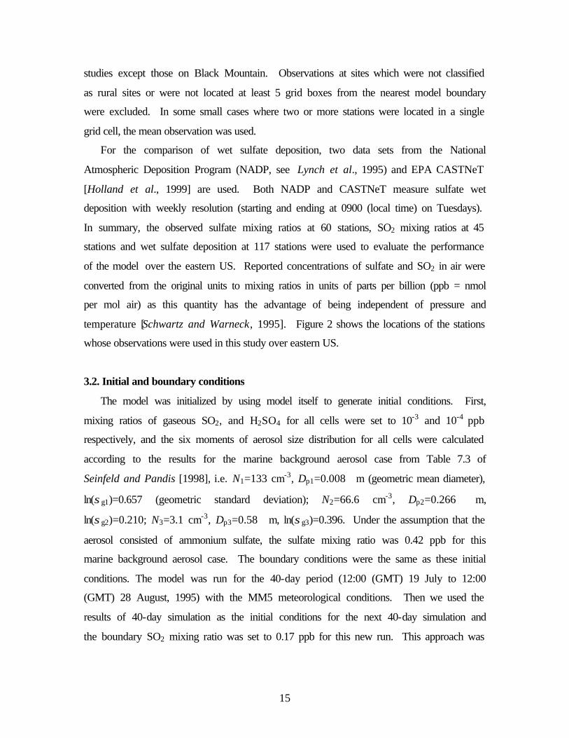
3.2. Initial and boundary conditions

The model was initialized by using model itself to generate initial conditions. First,

mixing ratios of gaseous SO2, and H2SO4 for all cells were set to 10-3 and 10-4 ppb

respectively, and the six moments of aerosol size distribution for all cells were calculated

according to the results for the marine background aerosol case from Table 7.3 of

Seinfeld and Pandis [1998], i.e. N1=133 cm-3, Dp1=0.008 µm (geometric mean diameter),

ln(σg1)=0.657 (geometric standard deviation); N2=66.6 cm-3, Dp2=0.266 µm,

ln(σg2)=0.210; N3=3.1 cm-3, Dp3=0.58 µm, ln(σg3)=0.396. Under the assumption that the

aerosol consisted of ammonium sulfate, the sulfate mixing ratio was 0.42 ppb for this

marine background aerosol case. The boundary conditions were the same as these initial

conditions. The model was run for the 40-day period (12:00 (GMT) 19 July to 12:00

(GMT) 28 August, 1995) with the MM5 meteorological conditions. Then we used the

results of 40-day simulation as the initial conditions for the next 40-day simulation and

the boundary SO2 mixing ratio was set to 0.17 ppb for this new run. This approach was

16

taken so as not to bias the model to low concentration that would result if the model run

were initialized with low background concentrations.

3.3. Evaluation of model and discussions

3.3.1. Time-series comparisons at the Great Smoky Mountains (GSM) and at the

Black Mountain, North Carolina

This section compares time-series of modeled and observed moments, mass

concentration and size parameters. Figure 2 shows the time-series of observed and

modeled sulfate mass and the synoptic conditions at the GSM location during the SEAVS

period [Sherman et al., 1997; Ames et al., 2000]. The dominant synoptic feature during

this period was Hurricane Erin, which made landfall around August 2, 1995. As shown

in Figure 2c, the model captured the buildup of observed sulfate mass from August 9 to

13, a dip during August 15-16, and a peak during August 17-18. However, the model

underpredicted slightly sulfate mass peak after the Hurricane and overpredicted slightly

the sulfate mass concentrations before and during the Hurricane Erin (Figure 2c).

For comparison of aerosol number concentration, moments and size parameters, one

should bear in mind that the model simulates sulfate only whereas the observed moments

and size distributions are for all aerosol species. Figure 3 shows that there were large

variations of observed six moments at the GSM during the SEAVS period. The

observed moments except µ0 were very high during the dust (July 23 to 26) and peak

(August 13 to 19) periods, especially for µ4 and µ5, when compared to other periods. As

compared to the observations in Figure 3, the model generally performs much better on

the low moments (µ0, and µ1) than high moments (µ4 and µ5) at the GSM. The mean

modeled number concentrations are 1516 cm-3 for the base case, somewhat higher than

the mean observed number concentration (1139 cm-3). The measurements determined

the number size distributions only between 0.05 µm and 0.125 µm, leading to possible

underestimate of the actual number concentration (zeroth moment). The first panel of

Figure 4 for the number concentration (µ0) shows that the model has similar magnitude to

the observations and captured the increase trends of the observed number concentrations

during August 10 and August 17 at the site. The model seriously underpredicts the high

moments, especially for µ4 and µ5, during the periods of dust (July 23 to 26) and high

17

concentrations (August 13 to 19). These underpredictions are attributed to the

contributions of large particles of aerosol species other than sulfate in the observed

particles as analyzed below. The soil mass concentration of the fine aerosol

(diameter<2.5 µm) was the highest for the whole study during the dust event, indicating

the likely presence of large particles [Sherman et al., 1997]. The OC concentrations

increased dramatically during the transition and peak period (July 8-18).

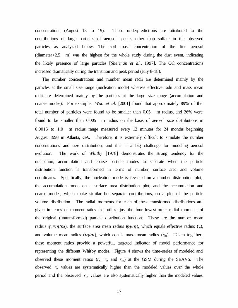
The number concentrations and number mean radii are determined mainly by the

particles at the small size range (nucleation mode) whereas effective radii and mass mean

radii are determined mainly by the particles at the large size range (accumulation and

coarse modes). For example, Woo et al. [2001] found that approximately 89% of the

total number of particles were found to be smaller than 0.05 µm radius, and 26% were

found to be smaller than 0.005 µm radius on the basis of aerosol size distributions in

0.0015 to 1.0 µm radius range measured every 12 minutes for 24 months beginning

August 1998 in Atlanta, GA. Therefore, it is extremely difficult to simulate the number

concentrations and size distribution, and this is a big challenge for modeling aerosol

evolution. The work of Whitby [1978] demonstrates the strong tendency for the

nucleation, accumulation and coarse particle modes to separate when the particle

distribution function is transformed in terms of number, surface area and volume

coordinates. Specifically, the nucleation mode is revealed on a number distribution plot,

the accumulation mode on a surface area distribution plot, and the accumulation and

coarse modes, which make similar but separate contributions, on a plot of the particle

volume distribution. The radial moments for each of these transformed distributions are

given in terms of moment ratios that utilize just the four lowest-order radial moments of

the original (untransformed) particle distribution function. These are the number mean

radius (rn=µ1/µ0), the surface area mean radius (µ3/µ2), which equals effective radius (re),

and volume mean radius (µ4/µ3), which equals mass mean radius (rm). Taken together,

these moment ratios provide a powerful, targeted indicator of model performance for

representing the different Whitby modes. Figure 4 shows the time-series of modeled and

observed these moment ratios (re, rn and rm) at the GSM during the SEAVS. The

observed rn values are systematically higher than the modeled values over the whole

period and the observed rm values are also systematically higher than the modeled values

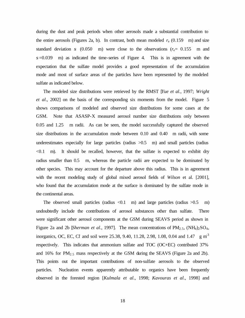
18

during the dust and peak periods when other aerosols made a substantial contribution to

the entire aerosols (Figures 2a, b). In contrast, both mean modeled re (0.159 µm) and size

standard deviation σ (0.050 µm) were close to the observations (re= 0.155 µm and

σ=0.039 µm) as indicated the time-series of Figure 4. This is in agreement with the

expectation that the sulfate model provides a good representation of the accumulation

mode and most of surface areas of the particles have been represented by the modeled

sulfate as indicated below.

The modeled size distributions were retrieved by the RMST [Yue et al., 1997; Wright

et al., 2002] on the basis of the corresponding six moments from the model. Figure 5

shows comparisons of modeled and observed size distributions for some cases at the

GSM. Note that ASASP-X measured aerosol number size distributions only between

0.05 and 1.25 µm radii. As can be seen, the model successfully captured the observed

size distributions in the accumulation mode between 0.10 and 0.40 µm radii, with some

underestimates especially for large particles (radius >0.5 µm) and small particles (radius

<0.1 µm). It should be recalled, however, that the sulfate is expected to exhibit dry

radius smaller than 0.5 µm, whereas the particle radii are expected to be dominated by

other species. This may account for the departure above this radius. This is in agreement

with the recent modeling study of global mixed aerosol fields of Wilson et al. [2001],

who found that the accumulation mode at the surface is dominated by the sulfate mode in

the continental areas.

The observed small particles (radius <0.1 µm) and large particles (radius >0.5 µm)

undoubtedly include the contributions of aerosol substances other than sulfate. There

were significant other aerosol components at the GSM during SEAVS period as shown in

Figure 2a and 2b [Sherman et al., 1997]. The mean concentrations of PM2.5, (NH4)2SO4,

inorganics, OC, EC, Cl- and soil were 25.38, 9.40, 11.28, 2.98, 1.08, 0.04 and 1.47 µg m-3

respectively. This indicates that ammonium sulfate and TOC (OC+EC) contributed 37%

and 16% for PM2.5 mass respectively at the GSM during the SEAVS (Figure 2a and 2b).

This points out the important contributions of non-sulfate aerosols to the observed

particles. Nucleation events apparently attributable to organics have been frequently

observed in the forested region [Kulmala et al., 1998; Kavouras et al., 1998] and

19

industrialized agricultural regions [Birmili and Wiedensohler, 1998]. In the chemical

analysis of the particles smaller than 0.25 µm radius in connection with the increase of

the Aitken nuclei over a forested area, Kavouras et al. [1998] found the existence of

organic acids (such as pinonic, formic and acetic acids), which are formed as oxidation

productions of gaseous monoterpenes emitted by the forest. The importance of the

anthropogenic hydrocarbons in the formation of secondary organic aerosol was also

emphasized by Odum et al. [1997]. Organics have been found to contribute substantially

to aerosol optical depths over the eastern coast of US [Hegg et al., 1997]. The results of

Figure 5 can be interpreted as suggesting the presence of non-sulfate particles in both

radius <0.1 µm (nucleation mode) (perhaps organics, which are heavy in the region as

shown in Figure 2b) and radius>0.5 µm (perhaps organics and soil) that are not included

in the sulfate model. This is consistent with the previous analyses for the moments in

Figure 3 and size parameters in Figure 4. Discrepancy between model and observations

might also arise from inaccuracy in the treatment of nucleation and of primary sulfate

emissions.

Figure 6 shows the time-series of modeled and observed six moments at Black

Mountain, North Carolina, during August 15-28, 1995. The model captures the general

magnitudes of observed six moments with better performance on µ1 and µ2. There are

similar explanations for the discrepancy between the model and observations for size

parameters at Black Mountain as those at GSM when we retrieve the size distributions on

the basis of the modeled six moments (not shown). Note that the TSI DMPS measured

aerosol particles only over the radius range from 0.008 to 0.3 µm at Black Mountain as

mentioned before, and the Black Mountain site (36 N, 82 W) is close to the GSM (36 N,

84W).

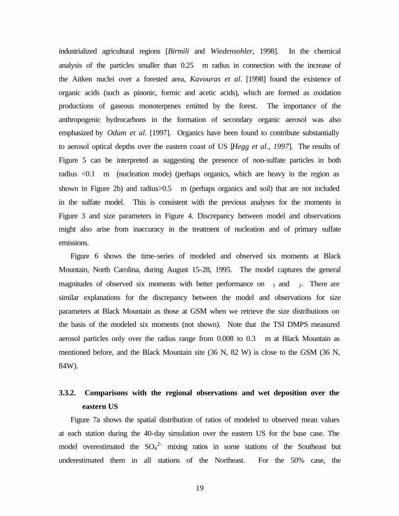
3.3.2. Comparisons with the regional observations and wet deposition over the

eastern US

Figure 7a shows the spatial distribution of ratios of modeled to observed mean values

at each station during the 40-day simulation over the eastern US for the base case. The

model overestimated the SO42- mixing ratios in some stations of the Southeast but

underestimated them in all stations of the Northeast. For the 50% case, the

20

underestimation of sulfate mixing ratios in the Northeast was improved but the

overestimation of sulfate mixing ratios in Southeast was increased (Figure 7b). Figure 8

shows scatter plots of model versus the individual concentration measurements for sulfate

and SO2 mixing ratios and wet deposition fluxes. Following Kasibhatla et al. [1997], we

calculated the percentages of comparison points whose model results were within a factor

of 2 of the corresponding measurements for each parameter. The results are listed in

Table 1. The domain averages for the comparison points were also calculated. As can be

seen, about half of the observed sulfate mixing ratios were simulated to within a factor of

2, and the domain average of the modeled sulfate mixing ratios for the base run was 13%

lower than the observation. Only ~25% of the sulfate wet deposition amounts were

simulated to within a factor of 2, and the domain average of the model results was 76%

higher than the observation for the base run. Although the modeled domain average of

sulfate wet deposition for the “50%” case was close to the observations (25%

overestimation) (Table 1), the “50%” case did not improve the model performance on the

wet deposition spatially as shown in Figures 7d and 8. The model seriously

overpredicted the sulfate wet deposition at most stations over the middle part of the

domain (Figure 7c, d). Overprediction of sulfate wet deposition may be one of reasons

leading to underprediction of sulfate mixing ratios over the Northeast (Figure 7a). The

scatterplot of Figure 8 indicates that the model overpredicted sulfate wet deposition more

when the observed sulfate wet deposition was less than 0.1 m mol m-2 week-1.

Inspection of Figures 7 and 8 shows that most of locations where ratios of modeled to

observed mean wet deposition was larger than 3.0 in Figure 7c and 7d were locations of

low sulfate deposition. As noted by Benkovitz and Schwartz [1997], departure of

modeled and observed values may not be attributed entirely to performance of the model

because the observed values at a station are not necessarily representative of the grid cell

as a whole and may be not suitable for evaluation of the model, which means to represent

the mean values over the grid cell. In addition to the problem in the representativeness of

the observations at a single location for the grid cell as a whole, the discrepancy between

the modeled and observed wet deposition can be due to inaccuracy in the representation

of locations and amounts of precipitation in the meteorological forecast model (here,

MM5) that drives the chemical transport model and in the representation of wet removal

21

processes [Seaman, 2000]. Discrepancies between model and observations might be due

also to errors in boundary conditions, especially near the western edge of the model

domain. Nonetheless, these considerations suggest a need to improve the accuracy of wet

processes in the model.

For the sensitivity study with the doubled condensation rate, the domain averages of

the modeled SO42- mixing ratios for the 40-day simulation period were about 15% lower

than for the base case (Table 1), and sulfate wet deposition about 7% higher, resulting in

decreased overall model skill compared with observations. These changes are attributed

to a shift in sulfate mass loading from the nucleation mode to the accumulation mode

(diameter 0.1 to 1.0 µm). Most of sulfate aerosols, both in ambient and in present model,

are located in the accumulation mode, whereas sea salt, dust, etc., which are not included

in the model, are in the coarse mode, which would contribute little to surface area.

Evidently the surface area for condensation is already accurately represented by the

modeled sulfate without inclusion of coarse mode aerosol. This may be the major reason

why a doubling of the condensation rate to account for aerosol species other than sulfate

results in a decrease in model performance. As the accumulation mode is more efficiently

removed by wet deposition than the nucleation mode, shifting sulfate from the nucleation

mode to the accumulation mode enhances the removal rate.

It was found that the model performs better on the mean results of the 40-day period

than on individual measurements. For instance, ~60% of the observed mean sulfate

mixing ratios and ~53% of observed mean wet sulfate deposition were simulated to

within a factor of 2, higher than those of the individual measurements for the base case

(Table 1). These results are in agreement with the study of Dennis et al. [1993], who

found that the absolute difference between observations and model results decreased

rapidly for successively longer averaging period because of temporal noise in the dataset.

It also probably means that the location of the material is displaced because of

inaccuracies in the wind field of the meteorological driver, which would tend to average

out.

The model systematically overestimated the observed SO2 mixing ratios, as shown in

Figure 8. Only 22% of the observed SO2 mixing ratios were simulated to within a factor

of 2, and the modeled domain average was 138% higher than the observations (Table 1).

22

Preliminary evaluation results of EPA’s Models-3 CMAQ also found that SO2

predications were biased high by a factor of 2 [Mebust et al., 2002; R. Dennis, personal

communication, 2002]. The overpredictions of SO2 were caused mainly by the nighttime

overestimation of SO2 on the basis of comparison of hourly measurements of SO2 from

AIRS in 1990 with the CMAQ results [R. Dennis, personal communication, 2002]. A

possible reason is the model’s coarse vertical resolution that cannot adequately resolve

sharp nocturnal gradients near the surface [J. Pleim, personal communication, 2002].

The overestimation of nighttime SO2 will not lead to substantial overestimation of gas-

phase oxidation of SO2 during nighttime but may lead to overestimation of aqueous phase

oxidation. At the GSM during the SEAVS period, we also found that the average of the

model results for SO2 (2.23 ppb) was much higher than the mean observed SO2

concentration (0.31 ppb) measured by the IMPROVE (filter sampler of the National Park

Service (NPS)) and that (0.92 ppb) measured by the HEADS (using Harvard-EPA

annular denuder system) during the SEAVS period [Andrews et al., 2000]. Andrews et

al. [2000] ascribed the systematically lower SO2 value (0.31 ppb) measured by the

IMPROVE to absorption of SO2 by the 8-foot aluminum inlet tube used in the IMPROVE

sampler. This result suggests that some systematically lower SO2 values of measurement

methods may also be one of the reasons that lead to low observed SO2 values compared

to the model. SO2 mixing ratios are also overpredicted in several global models

[Kasibhatla et al., 1997; Barth et al., 2000; Chin et al., 2000]. The additional possible

reasons for the overestimation of SO2 mixing ratios have been suggested: (1) additional

heterogeneous mechanisms for the oxidation of SO2 in the boundary layer; (2) non-

representative locations and elevations of surface observation sites. Most of SO2 is

released from stacks above local shallow inversion layers, with the observation stations

located close to the surface below the inversions.

3.3.3. Comparisons of vertical profiles of mass and number concentrations and size

distributions with measurements over Nashville, Tennessee

The comparisons of modeled and observed vertical profiles of sulfate mass

concentrations and size parameters over the Tennessee provide an assessment for the

ability of the model to represent vertical structure of aerosol properties. In this study, the

23

data of two periods (period 1: 14:00-18:00 (GMT) July 19, 1995 and period 2: 12:00-

16:00 (GMT) July 20, 1995) from the SOS experiment over Nashville, Tennessee, are

used to compare with the model results of the base case. In order to compare the

modeled and observed vertical profiles, the observed and modeled size distribution data

were grouped according to the altitudes and longitudes and latitudes of the observations,

and corresponding layer heights and longitudes and latitudes of the model grid cells for

each period. The corresponding mean aerosol properties and SO2 mixing ratios were

calculated for each layer for the each period over the whole study region.

Figures 11 and 12 show the modeled and observed vertical profiles of mean sulfate

mixing ratios, number concentrations, re, rm, rn and SO2 mixing ratios as a function of

height (pressure) over Tennessee for the periods 1 and 2, respectively. For period 1, the

model generally captured the vertical variation patterns of the observed sulfate and SO2

mixing ratios, number concentration and rn as shown in Figure 11, especially for the

highest SO2 mixing ratio in the plumes at around 910 hPa. For period 2, the model

captures the vertical variation patterns of sulfate mixing ratios and rn well but poorly for

other parameters as shown in Figure 10. Specifically, The model underpredicted the

sulfate mixing ratios at low layers and high layers for both periods (Figures 9b and 10b).

The model overpredicted SO2 mixing ratios at low model layers for both periods but did

not capture the observed SO2 peak at around 910 hPa for period 2 (Figure 10f). This is

consistent with those in section 3.3.1 that the model underpredicts the sulfate a little but

overpredicts SO2 by a factor of 2 at the ground layer.

Figures 9d and 10d indicate that the modeled mass mean radii are systematically

smaller than the corresponding observations for both periods. As the observed aerosol

size distributions are available between 0.05 and 1.75 µm particle radius in 15 size-bins

measured by PCASP, we compared the mean observed size distributions with the

surrogates to the size distributions retrieved by the RMST [Yue et al., 1997; Wright et al.,

2002] on the basis of the corresponding mean six moments from the model. Figure 11

shows the examples of the comparisons of mean observed and modeled size distributions

at the layers 2 (982 hPa), 7 (943 hPa) and 12 (822 hPa) for the two periods. In most cases

the model has successfully captured the observed size distributions in the middle 6 bins

of accumulation mode (e.g. bins with radius boundaries of 0.10, 0.125, 0.15, 0.20, 0.25,

24

0.35, and 0.45 µm) which were determined mainly by sulfate aerosol. This result is in

agreement with the previous results obtained at the GSM (Figure 7). This is in agreement

with the recent finding of Brock et al. [2002] over Nashville during the SOS’ 99 field

mission that sulfate contributed most of the mass of aerosol particles in the plumes from

coal-fired power generation stations over Nashville on the basis of measurements of

submicrometer particle size distributions in the plumes and the calculations of a

numerical plume photochemistry model. Husar et al. [1978] also showed that sulfate

was predominant composition of aerosol particles formed in power plant plumes. Figure

11 shows that the retrieved number concentrations at the radii larger than 0.50 µm are

systematically lower than the observations for all layers like those at the GSM. However,

the model does not underpredict the observed particles in the small size range like those

at the GSM. For the SOS Nashville/Tennessee Field Intensive, one of its major goals

was to examine the role of power plant plumes in oxidation formation and the interaction

of these plumes with the Nashville urban plume [Hubler et al., 1998; McNider et al.,

1998]. The power plant plumes can be identified by increased SO2 concentrations

whereas the urban plume can be detected by elevated CO concentration [Brock et al.,

2002]. The very high mean SO2 concentrations at height of ~900 mb in both Figures 9f

and 11f indicate that both periods were strongly influenced by the power plant plumes.

This means that on the contrary to the observations at the GSM, the air masses in these

two periods over Nashville contained substantial portions of material directly emitted by

the power plants. Therefore, it is not surprising that the observed aerosol size

distributions contained some large particles (radius>0.5 µm) that may be not sulfate in

the two periods as shown in Figure 11. This can explain the systematic underprediction

of mass mean radius (Figures 9d and 10d) because the large particles other than sulfate in

observations can make a substantial contribution to mass mean radius. This may be the

reason that Von Salzen et al. [2000] also found their modeled mean mass radii based on

the sulfate smaller than the observations over the Tennessee as well.

25

4. Spatial distributions of microphysical properties of aerosols over the eastern US

during summer

One of major goals of this model is to simulate aerosol microphysical properties over

the eastern US. Since our results were based only on the 40-day simulation from July 19

to August 28, 1995 and there was a Hurricane Erin even during the period, it needs to

consider these extreme meteorological conditions when compared to other model’s

results. Figure 12 shows the horizontal spatial distributions of the 40-day mean sulfate

mixing ratios and number concentrations at the lowest model layer over the eastern US

for the base case. As can be seen, the high sulfate mixing ratios are located around the

Ohio River valley, whereas the high number concentrations are located over the

Northeastern Coast (New Jersey area) as well as the Ohio River valley. This is generally

in agreement with the observations of eastern US PM2.5 and PM10 patterns [EPA, 1996],

in which the summer peaks (~40 µg m-3 for PM10 and ~24 µg m-3 for PM2.5) were

determined over the Ohio River valley where sulfate is a major component of PM. As

mass mean radii are available over eastern US in the modeling study of von Salzen et al.

[2000], it is of interest to compare our results with theirs, although a direct comparison of

the results of the two studies might not be appropriate because of different years (July 17-

30, 1995 in this study vs July 17 to 30, 1994 in von Salzen et al. [2000]). The mass mean

radius at ambient relative humidity in the present simulation is 0.15 ± 0.013 (one standard

deviation) µm, fairly close to but somewhat higher than the mean value obtained by von

Salzen et al. [2000] (0.11 ± 0.030 µm) for the corresponding cells over the eastern US.

Examination of the spatial distributions of mass mean radius from the two models did not

show evidence of strong spatial correlation. The reasons for this are not known—

differences in emissions, model, or controlling meteorology.

To better understand the sources and vertical profiles of sulfate properties, we

analyzed the sulfate aerosol properties and carried out process analysis at three specific

locations over New Jersey, Ohio River valley and Atlantic Ocean shown in Figure 12a.

Figure 13 shows the vertical profiles of mean number concentrations, sulfate, SO2 and

H2SO4 mixing ratios and mass mean radii for the three locations. As expected, both

mean sulfate mixing ratios and number concentrations over the Ohio River valley were

much higher than those over other two locations below layer 11 (~1.4 km). Somewhat

26

surprisingly, sulfate mixing ratios over the Atlantic Ocean location were greater than

those over the New Jersey below layer 6 (~340 m) whereas the number concentrations

over the Atlantic Ocean location were lower at the low model layers. This is consistent

with the larger mass mean radii over the Atlantic Ocean location (Figure 13). As

expected, both SO2 and H2SO4 vertical profiles were the lowest over the Atlantic Ocean

location. Because the number of layers used for emissions was limited to 14 (~2600 m)

in the model, the mean number concentrations, sulfate, SO2 and H2SO4 mixing ratios and

mass mean radii were very close for the three locations above layer 15 (Figure 13).

To better understand the contribution of each process to formation of sulfate aerosol,

we analyzed the column sulfate amount and number changes and their budget over the

three locations for the 40-day simulation (Table 2). 77% of total sulfate was located

below layer 14 (~2.6 km) over both New Jersey and Ohio River valley locations whereas

only 56% sulfate was located below layer 14 for the Atlantic Ocean location. Aqueous

phase reaction of SO2 is the dominant sulfate source, contributing 70% over both New

Jersey and Ohio River valley locations. This is close to those of Roelofs et al. [2001],

who found on the basis of the simulations of 11 global sulfur cycle models that the

contributions of aqueous phase oxidation of SO2 were 59-67% for eastern North

America. Over the Atlantic Ocean location, the aqueous reaction of SO2 even contributed

82% of total sulfate source because of no emission there. The contributions of gas-phase

reaction through condensation and nucleation to sulfate amount range from 18% over

both Atlantic Ocean and Ohio River valley locations to 17% over New Jersey location.

Wet deposition was a major sink over the three regions (Table 2). The wet deposition

was a major sink over the southern Atlantic Ocean (-98%), whereas it only contributed to

24% and 33% of total sink over the New Jersey and Ohio River valley respectively.

These results indicate that the contribution of each process to the sulfate mass fluxes can

vary greatly from one area to another area. The sulfate mass column amounts (Table 2)

were substantially higher than those of Kasibhatla et al. [1997] (~0.156 mmol m-2) and

Roelofs et al. [2001] (0.133 mmol m-2) on the basis of the global CTM simulations for

eastern North America in summer. However, as our results were for only 40-day period,

these results may be not comparable.

27

In contrast to the sulfate amount, the percentages of total number of particles located

below layer 14 (~2.6 km) were 59%, 48%, and 14% over Ohio River valley, New Jersey,

and Atlantic Ocean locations respectively. The major portion of sulfate mass was located

below 2.6 km whereas most of particle number was above 2.6 km except over Ohio River

valley location (Table 2). This is reasonable because the large particles with major mass

will exist at the low layers of the atmosphere and small particles with big contribution to

total number concentration will exist at the high layers of the atmosphere. As analyzed

by Adams and Seinfeld [2002], this vertical profile resulted from the higher nucleation

rate in the upper troposphere and tropopause region and was in agreement with the

observations of Schroder et al. [2002]. Over Ohio River valley, substantial portion of

number budget was located below 2.6 km (layer 14) because major emissions occurred

below 2.6 km over the area, and direct emissions were dominant sources of sulfate

number concentration as analyzed below. Direct emissions were the dominant sources of

particle number over both the New Jersey (99%) and Ohio River valley (96%) locations,

whereas nucleation was only source of particle number at the Atlantic Ocean locations as

listed in Table 2. As expected, coagulation was the dominant sink of particle number for

all locations. Note, at the Ohio River valley and New Jersey locations total production of

both sulfate amount and number substantially exceeds removal, whereas at the Atlanta

Ocean location total removal exceeds production (Table 2). This indicates that the

transport moved out substantial portion of the sulfate mass and number from the Ohio

River valley and New Jersey locations, but that there was net import of sulfate mass and

number into the Atlantic Ocean location. This is due to the fact that there was substantial

emission at the Ohio River valley and New Jersey locations, as well as substantial sulfate

formation by reaction, whereas at the Atlantic Ocean location there was no emission and

much less reaction.

The lifetime of sulfate number is much shorter than sulfate amount because of the

strong removal process of coagulation for the sulfate number (Table 2). For the three

studied locations, the lifetimes of both sulfate amount and number over the Atlantic

Ocean location (8.05 days for amount and 1.70 days for number) were much longer than

those over the New Jersey location (4.97 days for amount and 0.38 days for number) and

Ohio River valley location (2.56 days for mass and 0.17 days for number). The smaller

28

wet removal and coagulation rates over the Atlantic Ocean location lead to longer

lifetimes for sulfate amount and number respectively as shown in Table 2. The longer

lifetime of sulfate amount and number over the Atlantic Ocean may be another reason for

the particles to become bigger than other locations (Figure 13). In the results of Roelofs

et al. [2001], Kasibhatla et al. [1997] and Chin et al. [2000], the lifetimes of sulfate

amount were 2.0 to 5.4, 2.7 and 3.4 days for eastern North America respectively. Our

results seem consistent with these results, especially over the New Jersey and Ohio River

valley.

5. Summary and Conclusions

A six-moment aerosol microphysical module (6M) has been implemented in a

regional 3-D air quality model (MAQSIP) and applied to sulfate aerosol in the eastern US

for 40 day simulation of July to August 1995. The model successfully captured the

observed size distribution in the accumulation mode (radius 0.1 to 0.5 µm), in which the

sulfate is predominately located, on the basis of the size distributions retrieved from the

modeled six moments at the GSM during the SEAVS. These results demonstrate the

utility as well as the efficiencyof moment-based models. A one-day simulation needs ~8

hours computer time at a single-processor Sun (ULTRA 60) station. However, the model

did not predict some of the moments well, especially the higher moments and during the

dust events. Over the eastern US, the domain average of modeled SO42- mixing ratios

was 13% lower than the observations, with about 50% of the observations simulated to

within a factor of 2. One of reasons for this underestimation of sulfate mixing ratios is

thought to be overprediction of sulfate wet deposition. Reduction of the fraction of

sulfate taken into cloud water from 100% to 50% does not improve the model

performance spatially over the eastern US. The model systematically overestimated the

observed SO2 mixing ratios, by a factor of 2.4 on average.

The sensitivity test with doubled condensation rate suggests that most of the aerosol

surface area, determined mainly by the accumulation mode, is well represented by the

modeled sulfate. This is supported by the results that the model reproduced the effective

radii better than other size parameters. Over Nashville during the SOS, the model closely

reproduced the observed size distributions between 0.10 and 0.45 µm (dry radius), and

29

the observed and modeled sulfate mass concentrations are close as well. However, the

model seriously underpredicted the observed high moments of total aerosol size

distributions at the GSM during the periods when the site was influenced by the dust or

the air mass transported from the Ohio River valley. Comparison of the observed and

retrieved size distributions on the basis of the modeled six moments indicates that the

model underpredicts the observed large particles (radius>0.5 µm, coarse mode) and small

particles (radius<0.1 µm, nucleation mode) at the GSM and underpredicts the observed

large particles over Nashville as well. In-situ chemical analyses indicated that other

aerosol components such as dust and organics might make a substantial contribution to

the observed particles in these two size ranges. Errors in the representation of sulfate

nucleation or primary sulfate emissions might also cause these discrepancies, especially

for the nucleation mode.

On the basis of the simulation of sulfate aerosols, it was found that the highest sulfate

mass concentrations were located around the Ohio River valley whereas the high number

concentrations were located over the Northeastern Coast (New Jersey area) and Ohio

River valley. On the basis of column integral change and burden analysis of sulfate

amount and number over the three locations, it was found that the contribution of each

process varied considerably from one location to another location. The major portion of

sulfate mass was located below 2.6 km and most of sulfate number locates above 2.6 km

except over Ohio River valley where there was a major low-level input from emissions.

There are uncertainties in both quantitatively describing the aerosol dynamics and

microphysics and in other atmospheric processes such as advection and diffusion

represented in the model. Uncertainties in nucleation processes and rates are major

limiting factors in modeling particle number and thus the modeling of other aerosol

properties, for which knowledge of aerosol number size distributions is required. In light

of these uncertainties, the performance of our 6M moments-based module in the regional

model can be considered to successfully represent aerosol evolution and properties. On

the other hands, as shown in comparisons with observations over GSM and Nashville,

Tennessee, accurate representation of properties of the whole aerosol obviously must

include other important aerosol constituents such as dust and organics, especially for the

eastern US.

30

Acknowledgments. We thank Drs. S. Kreidenweis, W. Malm, B. Schichtel, J. Sisler, J.

Hand and R. Ames for providing IMPROVE and SEAVS datasets, Dr. R. Larson for

NADP data, Dr. L.I. Kleinman for the SOS dataset and Dr. K. von Salzen for the results

of the NARCM. We also thank U. Shankar and Dr. R. Mathur for supplying MAQSIP

model. We thank two anonymous referees for their helpful comments on the manuscript.

Work done at Duke was supported by grant NA76GP0350 from NOAA Office of Global

Programs, and Subcontract G-35-W62-G2 from Georgia Institute of Technology

(Principal grant R 826372-01-0 from EPA). Work done at BNL was supported in part by

NASA through interagency agreement number W-18,429 as part of its interdisciplinary

program on tropospheric aerosols, and in part by the Environmental Sciences Division of

the U.S. Department of Energy (DOE) as part of the Atmospheric Chemistry Program,

and was performed under the auspices of DOE under Contract No. DE-AC02-

98CH10886.

References

Abdul-Razzak, H., S. J. Ghan, and C. Rivera-Carpio, A parameterization of aerosol

activation 1. Single aerosol type, J. Geophys. Res. 103, 6123-5131, 1998.

Adams, P.J., and J.H. Seinfeld, Predicting global aerosol size distributions in general

circulation models. J. Geophys. Res., 107(D19), 4370, doi: 10.1029/2001JD001010,

2002.

Ames, R.B., J.L. Hand, S.M. Kreidenweis, D.E. Day, and W.C. Malm, Optical

measurements of aerosol size distributions in Great Smoky Mountains National Park:

Dry aerosol characterization, J. Air & Waste Manage. Assoc., 50, 665-676, 2000.

Andrews, E., P. Saxena, S. Musarra, L.M. Hildemann, P. Koutrakis, P.H. McMurry, I.

Olmez, and W.H. White, Concentration and composition of atmospheric aerosols

from the 1995 SEAVS experiment and a review of the closure between chemical and

gravimetric measurements, J. Air & Waste Manage. Assoc., 50, 648-664, 2000.

Barrett, J. C. and N. A. Webb, A comparison of some approximate methods for solving

the aerosol general dynamic equation, J. Aerosol Sci. 29, 31-39, 1998.

31

Benkovitz, C.M., and S.E. Schwartz, Evaluation of modeled sulfate and SO2 over North

America and Europe for four seasonal months in 1986-1987. J. Geophys. Res. 102,

25,305-25,338, 1997.

Binkowski, F.S., and U. Shankar, The regional particulate model 1: Model description

and preliminary results. J. Geophys. Res. 100, 26191-26209, 1995.

Birmili, W., and A. Wiedensohler, The influence of meteorological parameters on

ultrafine particle production at a continental site. J. Aerosol Sci., 29, S1015-1016,

1998.

Brock, C.A.,R.A. Washenfelder, M. Trainer, T.B. Ryerson, J.C. Wilson, J.M. Reeves,

L.G. Huey, J.S. Holloway, D.D. Parrish, G. Hubler, and F.C. Fehsenfeld, Particle

growth in the plumes of coal-fired power plants. J. Geophys. Res., 2002 (in press)

Byun, D.W., and J.K.S. Ching, Science algorithms of the EPA Models-3 community

multiscale air quality (CMAQ) modeling system. USA EPA/600/R-99/030, 1999.

Chin, M., D.L. Savoie, B.J. Huebert, A.R. Bandy, D.C. Thornton, T. S. Bates, P.K.

Quinn, E.S. Saltzman, and W.J. Bruyn, Atmospheric sulfur cycle simulated in the

global model GOCART: Comparison with field observations and regional budgets. .

J. Geophys. Res. 105, 24,689-24,712, 2000.

Chang, J.S., R.A. Brost, I.S.A. Isaksen, S. Madronich, P. Middleton, W.R. Stockwell, and

C.J. Walcek, A three-dimensional Eulerian acid deposition model: Physical concepts

and formation, J. Geophys. Res., 92, 14681-14700, 1987.

Chang, J.S., P. Middleton, W.R. Stockwell, C.J. Walcek, J.E. Pleim, H.H. Lansford, F.S.

Binkowski, S. Madronich, N.L. Seaman, D.R. Stauffer, D. Byun, J.N. McHenry, P.J.

Samson, and H. Hass, The regional acid deposition model and engineering model,

Acidic Deposition: State of Science and Technology, Report 4, National Acid

Precipitation Assessment Program, 1990.

Dana, M.T., and J.M. Hales, Statistical aspects of the washout of polydispers aerosols,

Atmos. Environ., 10, 45-50, 1976

Daum, P.H., T.J. Kelly, S.E. Schwartz and L. Newman, Measurements of the chemical

composition of stratiform clouds. Atmos. Environ., 18, 2671-2684, 1984a.

Daum, P.H., S.E. Schwartz and L. Newman, Acidic and related constituents in liquid

water stratiform clouds. J. Geophys. Res., 89, 1447-1458, 1984b

32

DeMore, W.B., S.P. Sander, D.M. Golden, R.F. Hampson, M.J. Kurlo, C.J. Howard, A.R.

Ravishankara, C.E. Kolb, and M.J. Molina, Chemical kinetics and photochemical

data for use in stratospheric modeling, JPL Publ., 92-20, 1992.

Dennis, R.L., J.N. McHenry, W.R.Barchet, F.S. Binkowski, and D.W. Byun, Correcting

RADM’s sulfate underprediction: Discovery and correction of model errors and

testing the corrections through comparisons against field data. Atmos. Environ., 26

A(6), 975-997, 1993.

Draxler, R. R. and G. D. Hess (1998) An Overview of The HYSPLIT_4 Modeling

System for Trajectories, Dispersion and Deposition. Aus. Met. Mag., 47: 295-308.

Environmental Protection Agency (EPA), Air Quality Criteria for Particular Matter,

EPA/600/P-95/001aF, 1996

Feller, W., An introduction to probability theory and its applications Vol. 2, Wiley, New

York, 1971, page 155.

Fitzgerald, J. W., W. A. Hoppel and F. Gelbard, A one-dimensional sectional model to

simulate multicomponent aerosol dynamics in the marine boundary layer I. Model

description, J. Geophys. Res., 103, 16,085-16,102 1998.

Fuchs, N. A., The Mechanics of Aerosols (translated by Daisley, R. E., and Fuchs, M.),

Pergamon Press, New York, 1964.

Ghan, S. J., R.C. Easter, E.G. Chapman, H. Abdul-Razzak, Y. Zhang, L.R. Leung, N.S.

Laulainen, R.D. Saylor, and R.A. Zaveri, A physically based estimate of radiative

forcing by anthropogenic sulfate aerosol. J. Geophys. Res., 106, 5279-5293, 2001.

Gery, M.W., G.Z. Whitten, J.P. Killus, and M.C. Dodge, A photochemical kinetics

mechanism for urban and regional scale computer modeling, J. Geophys. Res., 94,

12925-12956, 1989.

Giorgi, F., A particle dry-deposition parameterization scheme for use in tracer transport

models, J. Geophys. Res. 91, 9794-9806, 1986.

Grell, G.A., J. Dudhia and D.R. Stauffer, A description of the Fifth-Generation Penn

State/NCAR Mesoscale Model (MM5), Rep. NCAR/TN-389+STR, 138 pp., Natl.

Cent. For Atmos. Res., Boulder, Colo., 1994

33

Hegg, D.A., J. Livingston, P.V. Hobbs, T. Novakov, and P. Russell, Chemical

apportionment of aerosol column optical depth off the mid-Atlantic coast of the

United States. J. Geophys. Res. 102, 25297-25303, 1997

Hicks, B.B., T.P. Meyers, R.P. Hosker Jr., R.S. Artz, Climatological features of regional

surface air quality from the Atmospheric Integrated Research Monitoring Network

(AIRMoN) in the USA, Atmos. Environ., 35, 1053-1068, 2001.

Houyoux, M.R., J.M. Vukovich, C.J. Coats Jr., N.M. Wheeler, and P.S. Kasibhatla,

Emission inventory development and processing for the seasonal model for regional

air quality (SMRAQ) project. J. Geophys. Res. 105, 9079-9090, 2000.

Holland, D.M., P.P. Principe, J.E. Sickles II, Trends in atmospheric sulfur and nitrogen

species in the eastern United States for 1989-1995. Atmos. Environ., 33, 37-49, 1999.

Hubler, G., et al., An overview of the airborne activities during the Southern Oxidants

Study (SOS) 1995 Nashville/Middle Tennessee Ozone Study. J. Geophys. Res., 103,

22245-22259, 1998.

Husar, R.B., D.E. Patterson, J.D. Husar, N.V. Gillani, and W.E. Wilson, Jr., Sulfur

budget of a power plant plume, Atmos. Environ., 12, 549-568, 1978.

Jacobson, M. Z., R. P. Turco, E. J. Jensen, and O. B. Toon, Modeling coagulation among

particles of different composition and size, Atmos. Environ. 28, 1327-1338, 1994.

Jacobson, M.Z., Analysis of aerosol interactions with numerical techniques for solving

coagulation, nucleation, condensation, dissolution, and reversible chemistry among

multiple size distributions. J. Geophys. Res., 107 (D19), 4366, doi:

10.1029/2001JD002044, 2002.

Jaecker-Voirol, A., and P. Mirabel, Heteromolecular nucleation in the sulfuric acid-water

system, Atmos. Environ. 23, 2053-2057, 1989.

Jang, J.C., H.E. Jeffries, D. Byun, and J. Pleim, Sensitivity of ozone to model grid

resolution-I. Application of high-resolution regional acid deposition model. Atmos.

Environ., 29, 3085-3100, 1995.

Kasibhatla, P., Chameides, W.L., and S.S. John, A three-dimensional global model

investigation of seasonal variations in the atmospheric burden of anthropogenic

sulfate aerosols, J. Geophys. Res., 102, 3737-3759, 1997a.

34

Kasibhatla, P., Chameides, W.L., B. Duncan, M. Houyoux, C. Jang, R. Mathur, T.

Odman, and A. Xiu, Impact of inert organic nitrate formation on ground-level ozone

in a regional air quality model using the carbon Bond Mechanism 4, Geophys. Res.

Lett., 24, 3205-3208, 1997b.

Kasibhatla, P., and W.L. Chameides, Seasonal modeling of regional ozone pollution in

the eastern United States. Geophys. Res. Lett., 27, 1415-1418, 2000.

Kavouras, I.G., N. Mihalopoulos, and E.G. Stephanou, Formation of atmospheric

particles from organic acids produced by forests. Nature, 395, 683-686, 1998.

Koch, D., D. Jacob, I. Tegen, D. Rind, and M. Chin, Tropospheric sulfate simulation and

sulfate direct radiative forcing in the Goddard Institute for Space Studies general

circulation model. J. Geophys. Res., 104, 23799-23822, 1999.

Kreidenweis, S.M., J.E. Penner, F. Yin, and J.H. Seinfeld, The effects of dimethylsulfide

upon marine aerosol concentrations, Atmos. Environ. 25, 2501-2511, 1991.

Kuo, Y.-H., Further studies of the parameterization of the influence of cumulus

convection on large-scale flow, J. Atmos. Sci., 31, 1232-1240, 1974

Kulmala, M., A. Toivonen, J.M. Makela, and A. Laaksonen, Analysis of the growth of

nucleation mode particles observed in Boreal forest, Tellus, 50B, 449-462, 1998.

McGraw R. and J.H. Saunders, A condensation feedback mechanism for oscillatory

nucleation and growth, Aerosol Sci. and Technol. 3, 367-380, 1984.

McGraw R., Description of aerosol dynamics by the quadrature method of moments,

Aerosol Sci. Technol. 27, 255-265, 1997.

McNider, R.T., W.B. Norris, A.J. Song, R.L. Clymer, S. Gupta, R.M. Banta, R.J.

Zamora, A.B. White, and M. Trainer, Meteorological conditions during the 1995

Southern Oxidation Study Nashville/Middle Tennessee field intensive, J. Geophys.

Res. 103, 22,225-22,243, 1998.

Mebust, M.R., B.K. Eder, F.S. Binkowski, and S.J. Roselle, Models-3 community

multiscale air quality model (CMAQ) aerosol component 2. Model evaluation, J.

Geophys. Res., 2002 (in press).

Langner, J., and H. Rodhe, A global three-dimensional model of the tropospheric sulfur

cycle. J. Atmos. Chem., 13, 225-263, 1991

35

Lynch, J.A., J.W. Grimm, and V.C. Bowersox, Trends in precipitation chemistry in the

United States, a national perspective, 1980-1992. Atmos. Environ., 29, 1231-1246,

1995

Odman, M.T., and C.L. Ingram, Technical report: Multiscale Air Quality Simulation

Platform (MAQSIP): Source code documentation and validation, Rep. ENV-

96TR002-v1.0., 83 pp., MCNC Environ. Programs, Research Triangle Park, N.C.,

1996.

Ogren, J.A., Asystematic approach to In Situ observations of aerosol properties. In

Aerosol Forcing of Climate. Charlson, R.J., and Heintzenberg, J., Eds., pp. 215-226.

Wiley, New York, 1995.

Penner, J. E., and coauthor, A comparison of model- and satellite-derived aerosol optical

depth and reflectivity. J. Atmos. Sci., 59, 441-460, 2002.

Rasch, P.J., M.C. Barth, J.T. Kiehl, S.E. Schwartz, and C.M. Benkovitz, A description of

the global sulfur cycle and its controlling processes in the National Center for

Atmospheric Research Community Climate Model, Version 3. J. Geophys. Res. 105,

1367-1385, 2000.

Roelofs, G.J., P. Kasibhatla, L. Barrie, D. Bergmann, C. Bridgeman, M. Chin, J.

Christensen, R. Easter, J. Feichter, A. Jeuken, E. Kjellstrom, D. Koch, C. Land, U.

Lohmann, and P. Rasch, Analysis of regional budgets of sulfur species modeled for

the COSAM exercise, Tellus, 53, 673-694, 2001.

Russell, A., and R. Dennis, NARSTO critical review of photochemical models and

modeling, Atmos. Environ., 34, 2283-2324, 2000.

Russell, L., and J. H. Seinfeld, Size- and composition-resolved externally mixed aerosol

model, Aerosol Sci. and Technol. 28, 403-416, 1998.

Seaman, N.L., Meteorological modeling for air-quality assessments, Atmos. Environ., 34,

2231-2259, 2000

Schroder, F.P., B. Karcher, A. Petzold, and M. Fiebig, Aerosol sources and

transformation processes in the free troposphere and tropopause region at northern

midlatitudes, J. Geophys. Res., 107, doi: 10.1029/2000JD000194, 2002.

Schwartz, S.E., Mass-transport considerations pertinent to aqueous phase reactions of

gases in liquid-water clouds. In: Chemistry of Multiphase Atmospheric Systems,

36

Edited by W. Jaeschke, Springer-Verlag Berlin Heidelberg, NATO ASI Series, Vol.

G6, PP415-471, 1986

Schwartz, S.E., and P. Warneck, Units for use in atmospheric chemistry. Pure and

Applied Chemistry, 67, 1377-1406, 1995.

Schwartz, S. E., The whitehouse effect- Shortwave radiative forcing of climate by

anthropogenic aerosols: An overview, J. Aerosol Science, 27, 359-382, 1996

Seinfeld, J.H., and S.N. Pandis, Atmospheric Chemistry and Physics of Air Pollution,

1326 pp., John Wiley, New York, 1998.

Sherman, D.E., S. Kreidenweis, and T. McKee, The influence of synoptic and local

meteorological conditions on ambient particle concentrations during the southeastern

aerosol and visibility study (SEAVS), Cooperative Institute for Research in the

Atmosphere, Colorado State University and Latimer and Associates: Boulder, CO,

February 1997; ISSN #0737-5352-34.

Sisler, J.F., and W.C. Malm, Interpretation of trends of PM2.5 and reconstructed visibility

from the IMPROVE network, J. Air & Waste Manage. Assoc., 50, 775-789, 2000.

Tang, I. N. and H. R. Munkelwitz, Water activities, densities, and refractive indices of

aqueous sulfates and sodium nitrate droplets of atmospheric importance, J. Geophys.

Res. 99, 18,801-18,808, 1994.

Taylor, K.E., Summarizing multiple aspects of model performance in a single diagram, J.

Geophys. Res., 106, 7183-7192, 2001.

Von Salzen, K., H.G. Leighton, P.A. Ariya, L.A. Barrie, S.L. Gong, J.P. Blanchet, L.

Spacek, U. Lohmann, and L.I. Kleinman, Sensitivity of sulfate aerosol size

distribution and CCN concentrations over North America to SOx emissions and H2O2

concentrations. J. Geophys. Res. 105, 9741-9765, 2000.

Vukovich, F.M., A. Gilliland, A. Venkatram, and J. Sherwell, On performing long-term

predictions of ozone using the SOMS model. Atmos. Environ., 35, 569-578, 2001.

Walcek, C.J., and G.R. Taylor, A theoretical method for computing vertical distributions

of acidity and sulfate production within cumulus clouds. J.Atmos. Sci., 43, 339-355,

1986.

Whitby, E., and P. H. McMurry, Modal aerosol dynamics modeling, Aerosol Sci.

Technol. 27, 673-688, 1997.

37

Whitby, K., The physical characteristics of sulfur aerosols, Atmos. Environ. 12, 125-159,

1978.

Wilson, J., C. Cuvelier, and R. Raes, A modeling study of global mixed aerosol fields, J.

Geophys. Res., 106, 34081-34108, 2001

Woo, K.S., D.R. Chen, D.Y.H. Pui, and P.H. McMurry, Measurement of Atlanta aerosol

size distributions: observations of ultrafine particle events. Aerosol Sci. Technol.,34,

75-87, 2001.

Wright, D.L., Retrieval of optical properties of atmospheric aerosols from moments of

the particle size distribution. J. Aerosol Sci. 31, 1-18, 2000.

Wright, D.L., R. McGraw, C. M. Benkovitz, and S.E. Schwartz, Six-moment

representation of multiple aerosol populations in a sub-hemispheric chemical

transformation model, Geophys. Res. Lett., 27, 967-970, 2000

Wright, D. L., P.S. Kasibhatla, R. McGraw, and S.E. Schwartz. Description and

evaluation of a six-moment aerosol microphysical module for use in atmospheric

chemical transport models, J. Geophys. Res., 106, 20275-20291, 2001

Wright, D.L., S.C. Yu, P. S. Kasibhatla, R. McGraw, S.E. Schwartz, V.K. Saxena and

G.K. Yue, Retrieval of aerosol properties from moments of the particle size

distribution for kernels involving the step function: cloud droplet activation, J.

Aerosol Sci., 33, 319-337, 2002.

Yu, S.C., V.K. Saxena, B.N. Wenny, J.J. DeLuisi, G.K. Yue and I. V. Petropavlovskikh,

2000. A study of the aerosol radiative properties needed to compute direct aerosol

forcing in the southeastern US. J. Geophys. Res., 105, 24739-24749, 2000

Yu, S.C., C.S, Zender and V.K. Saxena, Direct radiative forcing and atmospheric

absorption by boundary layer aerosols in the southeastern US: model estimates on the

basis of new observations. Atmos. Environ., 35, 3967-3977, 2001

Yue G. K., J. Lu, V. A. Mohnen, P. -H. Wang, V. K. Saxena and J. Anderson, Retrieving

aerosol optical properties from moments of the particle size distribution, Geophys.

Res. Lett. 24, 651-654, 1997.

38

Appendix A: Calculations of weighting function for distributing the precipitation

rates to each layer

As mixing ratios of water vapor (qv), cloud water qc (ice, qi), rainwater qr (snow, qs)

mixing ratios (g kg-1) and meteorological parameters such as wind speed are generated by

the MM5, the weighting function for calculating the precipitation rates at each resolved

cloud layer can be based on this available information. The steps to get the weighting

function according to the equation for rainwater mixing ratios in the MM5 (Grell et al.,

1994) are as follows:

Step 1: the rates at which is cloud water is converted into precipitation through

autoconversion (PRC) and accretion (PRA) processes, and the evaporation of rain (PRE) are

determined as follows [Grell et al., 1994]:

)(1 critcRC qqkP −= (A1)

bcRA

bENaqP

+

+Γ=30

)3(41

λπ (A2)

])2/2/5(

)([)1(2

2/2/53/12/1

2210

bcRE

bS

af

fBA

SNP

+

+Γ++

−=λµ

ρλ

π (A3)

4/10 )(r

w

qNρ

ρπλ =

2

2

TRKL

Ava

w ρ=

χswqB

1=

ρχµ=cS

where the parameters (N0, a, b) of Marshall-Palmer size distributions for rain are: N0 = 8

x 106 m-4, a = 842 m1-b s-1, b = 0.8, f1 = 0.78, f2 = 0.32. Γ is the gamma function and µ

is the dynamic viscosity of air. χ is diffusivity of vapor in air (m2 s-1). ρ and wρ are the

densities of air and rain respectively. qcrit=0.5 g kg-1 and k1 =10-3 s-1. E is the collection

efficiency (1 for rain, 0.1 for snow). Lw is the latent heat of evaporation and Ka is the

thermal conductivity of air. Rv is the gas constant for water vapor (461.5 J kg-1 K-1) and T

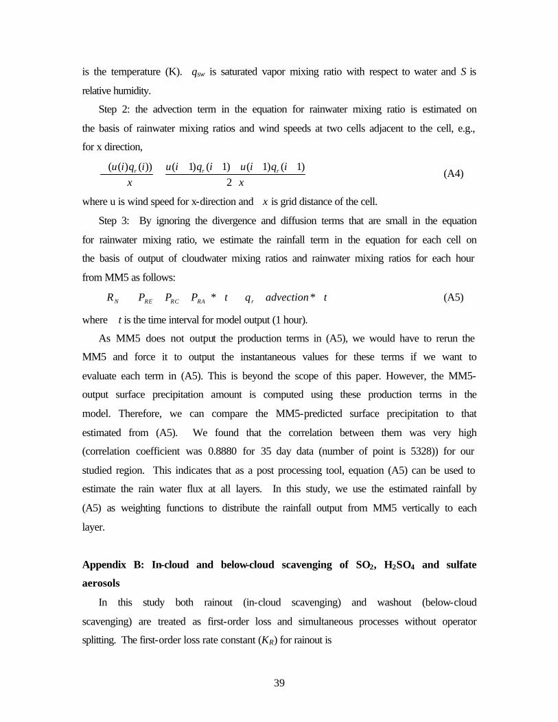
39

is the temperature (K). qsw is saturated vapor mixing ratio with respect to water and S is

relative humidity.

Step 2: the advection term in the equation for rainwater mixing ratio is estimated on

the basis of rainwater mixing ratios and wind speeds at two cells adjacent to the cell, e.g.,

for x direction,

xiqiuiqiu

xiqiu rrr

∆−−−++=

∆∆

2)1()1()1()1())()((

(A4)

where u is wind speed for x-direction and ∆x is grid distance of the cell.

Step 3: By ignoring the divergence and diffusion terms that are small in the equation

for rainwater mixing ratio, we estimate the rainfall term in the equation for each cell on

the basis of output of cloudwater mixing ratios and rainwater mixing ratios for each hour

from MM5 as follows:

( )[ ]tadvectionqtPPPR rRARCREN ∆−∆−∆++≅∆ ** (A5)

where t∆ is the time interval for model output (1 hour).

As MM5 does not output the production terms in (A5), we would have to rerun the

MM5 and force it to output the instantaneous values for these terms if we want to

evaluate each term in (A5). This is beyond the scope of this paper. However, the MM5-

output surface precipitation amount is computed using these production terms in the

model. Therefore, we can compare the MM5-predicted surface precipitation to that

estimated from (A5). We found that the correlation between them was very high

(correlation coefficient was 0.8880 for 35 day data (number of point is 5328)) for our

studied region. This indicates that as a post processing tool, equation (A5) can be used to

estimate the rain water flux at all layers. In this study, we use the estimated rainfall by

(A5) as weighting functions to distribute the rainfall output from MM5 vertically to each

layer.

Appendix B: In-cloud and below-cloud scavenging of SO2, H2SO4 and sulfate

aerosols

In this study both rainout (in-cloud scavenging) and washout (below-cloud

scavenging) are treated as first-order loss and simultaneous processes without operator

splitting. The first-order loss rate constant (KR) for rainout is

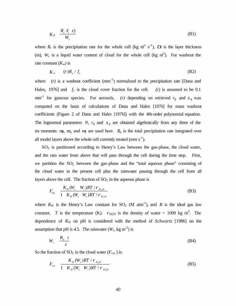
40

c

rR W

zRK

)/(∆= (B1)

where Rr is the precipitation rate for the whole cell (kg m-2 s-1), ∆z is the layer thickness

(m), Wc is a liquid water content of cloud for the whole cell (kg m-3). For washout the

rate constant (Kw) is

caw fRrK /)(Λ= (B2)

where Λ(r) is a washout coefficient (mm-1) normalized to the precipitation rate [Dana and

Hales, 1976] and fc is the cloud cover fraction for the cell. Λ(r) is assumed to be 0.1

mm-1 for gaseous species. For aerosols, Λ(r) depending on retrieved rg and σg was

computed on the basis of calculations of Dana and Hales [1976] for mass washout

coefficients (Figure 2 of Dana and Hales [1976]) with the 4th-order polynomial equation.

The lognormal parameters N, rg and σg are obtained algebraically from any three of the

six moments: µ0, µ1, and µ3 are used here. Ra is the total precipitation rate integrated over

all model layers above the whole cell currently treated (mm s-1).

SO2 is partitioned according to Henry’s Law between the gas-phase, the cloud water,

and the rain water from above that will pass through the cell during the time step. First,

we partition the SO2 between the gas-phase and the “total aqueous phase” consisting of

the cloud water in the present cell plus the rainwater passing through the cell from all

layers above the cell. The fraction of SO2 in the aqueous phase is

OHrcH

OHrcHaq RTWWK

RTWWKF

2

2

/)(1

/)(

ρρ

+++

= (B3)

where KH is the Henry’s Law constant for SO2 (M atm-1), and R is the ideal gas law

constant. T is the temperature (K). ρH2O is the density of water = 1000 kg m-3. The

dependence of KH on pH is considered with the method of Schwartz [1986] on the

assumption that pH is 4.5. The rainwater (Wr, kg m-3) is

ztR

W ar ∆

∆= (B4)

So the fraction of SO2 in the cloud water (Fcw ) is:

OHrcH

OHcHcw RTWWK

RTWKF

2

2

/)(1

/)(

ρ

ρ

++= (B5)

41

and the fraction of SO2 in the rain water (Frw) is:

OHrcH

OHrHrw RTWWK

RTWKF

2

2

/)(1

/)(

ρ

ρ

++= (B6)

The total SO2 concentration at time t ( )(][ 2 tSO tot ) in the grid cell is partitioned as

)(][ 2 tSO cw = Fcw )(][ 2 tSO tot

)(][ 2 tSO rw = Frw )(][ 2 tSO tot

)(][ 2 tSO g = (1 - Fcw - Frw) )(][ 2 tSO tot

where cw, rw and g represents cloud water, rainwater and gaseous phase respectively.

These concentrations are then updated as follows:

For rainout we have

)(][ 2 ttSO cw ∆+ = )(][ 2 tSO cw exp(- K R ∆t) (B7)

For washout the treatment depends on whether the process is limited by mass transfer

)(][ 2 ttSO rw ∆+ = )(][ 2 tSO rw exp(- wK ∆t) if Frw > 1 – exp(- wK ∆t)

with Λ(r) = 0.1 mm-1

or Henry’s Law equilibrium:

)(][ 2 ttSO rw ∆+ = )(][ 2 tSO rw (1 - Frw) if Frw < 1 – exp(- wK ∆t)

with Λ(r) = 0.1 mm-1

(B8)

The gas-phase portion remains unchanged by these processes as follows

)(][ 2 ttSO g ∆+ = )(][ 2 tSO g

The updated total SO2 concentration in cloudy portion of the cell is

)(][ 2 ttSO cld ∆+ = )(][ 2 ttSO cw ∆+ + )(][ 2 ttSO rw ∆+ + )(][ 2 ttSO g ∆+

If the cloud cover fraction (fc) is less than unity, the updated mean SO2 in the whole cell

is

)]([ 2 ttSO ∆+ = fc )(][ 2 ttSO cld ∆+ + (1 – fc ) )(][ 2 ttSO clr ∆+

where the updated SO2 concentration in clear-sky portion of the cell )(][ 2 ttSO clr ∆+ =

)]([ 2 tSO since at this point in the model integration clear-sky processes are not currently

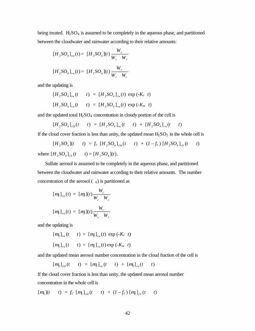
42

being treated. H2SO4 is assumed to be completely in the aqueous phase, and partitioned

between the cloudwater and rainwater according to their relative amounts:

)(][ 42 tSOH cw = )]([ 42 tSOHrc

c

WWW+

)(][ 42 tSOH rw = )]([ 42 tSOHrc

r

WWW+

and the updating is

)(][ 42 ttSOH cw ∆+ = )(][ 42 tSOH cw exp (-Kr∆t)

)(][ 42 ttSOH rw ∆+ = )(][ 42 tSOH rw exp (-Kw∆t)

and the updated total H2SO4 concentration in cloudy portion of the cell is

)(][ 42 ttSOH cld ∆+ = )(][ 42 ttSOH cw ∆+ + )(][ 42 ttSOH rw ∆+

If the cloud cover fraction is less than unity, the updated mean H2SO2 in the whole cell is

)]([ 42 ttSOH ∆+ = fc )(][ 42 ttSOH cld ∆+ + (1 – fc ) )(][ 42 ttSOH clr ∆+

where )(][ 42 ttSOH clr ∆+ = )]([ 42 tSOH .

Sulfate aerosol is assumed to be completely in the aqueous phase, and partitioned

between the cloudwater and rainwater according to their relative amounts. The number

concentration of the aerosol (µ0) is partitioned as

)(][ 0 tcwµ = rc

c

WWW

t+

)]([ 0µ

)(][ 0 trwµ = rc

r

WWW

t+

)]([ 0µ

and the updating is

)(][ 0 ttcw ∆+µ = )(][ 0 tcwµ exp (-Kr∆t)

)(][ 0 ttrw ∆+µ = )(][ 0 trwµ exp (-Kw∆t)

and the updated mean aerosol number concentration in the cloud fraction of the cell is

)(][ 0 ttcld ∆+µ = )(][ 0 ttcw ∆+µ + )(][ 0 ttrw ∆+µ

If the cloud cover fraction is less than unity, the updated mean aerosol number

concentration in the whole cell is

)]([ 0 tt ∆+µ = fc )(][ 0 ttcld ∆+µ + (1 – fc ) )(][ 0 ttclr ∆+µ

43

As the removal must be done after completing the microphysical processes, we save

the factor:

)]([

)(][

0

0

ttt

f cldfract µ

µ ∆+=

to represents the fraction of the aerosol remaining after rainout and washout in the cloudy

portion of cell. Note that this fraction of the aerosol was also applied to all six moments

because the moments of a PDF are not mathematically independent quantities as analyzed

in Section 2.2.

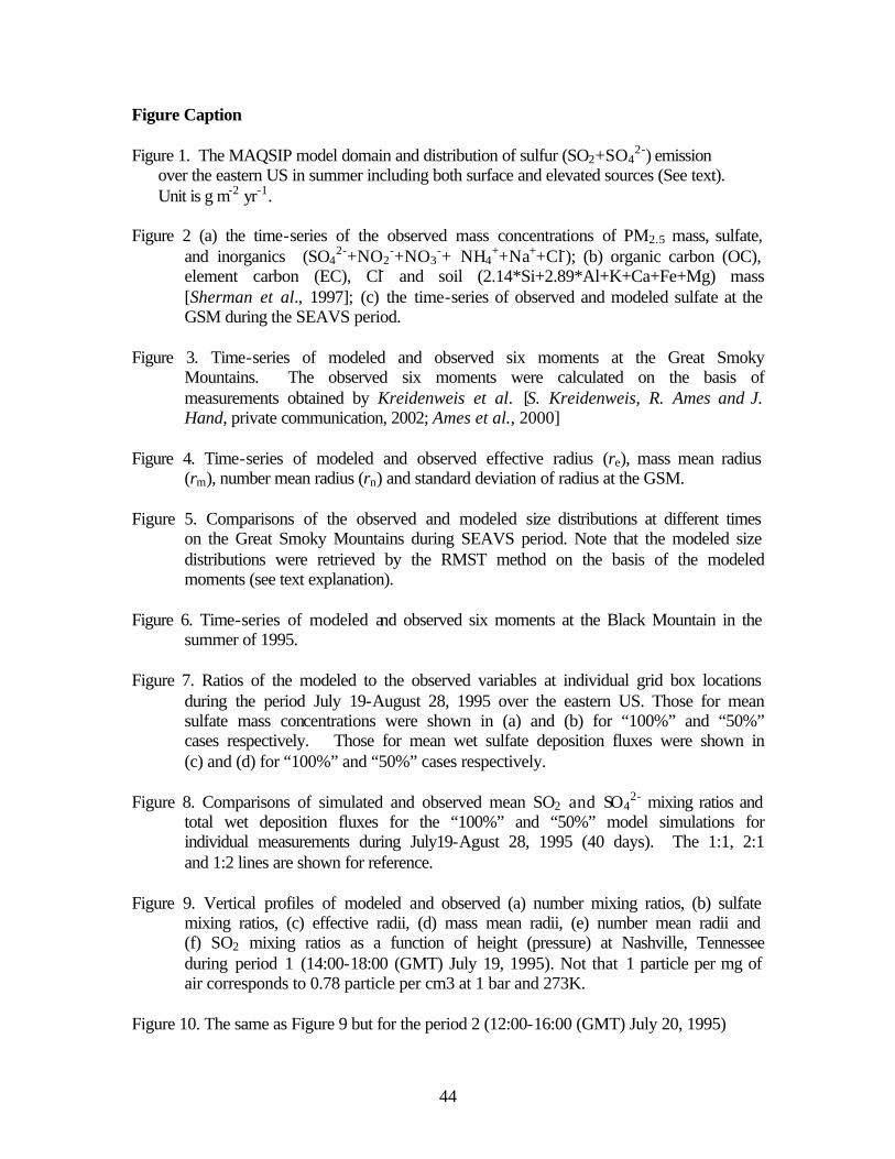
44

Figure Caption Figure 1. The MAQSIP model domain and distribution of sulfur (SO2+SO4

2-) emission over the eastern US in summer including both surface and elevated sources (See text). Unit is g m-2 yr-1.

Figure 2 (a) the time-series of the observed mass concentrations of PM2.5 mass, sulfate,

and inorganics (SO42-+NO2

-+NO3-+ NH4

++Na++Cl-); (b) organic carbon (OC), element carbon (EC), Cl- and soil (2.14*Si+2.89*Al+K+Ca+Fe+Mg) mass [Sherman et al., 1997]; (c) the time-series of observed and modeled sulfate at the GSM during the SEAVS period.

Figure 3. Time-series of modeled and observed six moments at the Great Smoky

Mountains. The observed six moments were calculated on the basis of measurements obtained by Kreidenweis et al. [S. Kreidenweis, R. Ames and J. Hand, private communication, 2002; Ames et al., 2000]

Figure 4. Time-series of modeled and observed effective radius (re), mass mean radius

(rm), number mean radius (rn) and standard deviation of radius at the GSM. Figure 5. Comparisons of the observed and modeled size distributions at different times

on the Great Smoky Mountains during SEAVS period. Note that the modeled size distributions were retrieved by the RMST method on the basis of the modeled moments (see text explanation).

Figure 6. Time-series of modeled and observed six moments at the Black Mountain in the

summer of 1995. Figure 7. Ratios of the modeled to the observed variables at individual grid box locations

during the period July 19-August 28, 1995 over the eastern US. Those for mean sulfate mass concentrations were shown in (a) and (b) for “100%” and “50%” cases respectively. Those for mean wet sulfate deposition fluxes were shown in (c) and (d) for “100%” and “50%” cases respectively.

Figure 8. Comparisons of simulated and observed mean SO2 and SO4

2- mixing ratios and total wet deposition fluxes for the “100%” and “50%” model simulations for individual measurements during July19-Agust 28, 1995 (40 days). The 1:1, 2:1 and 1:2 lines are shown for reference.

Figure 9. Vertical profiles of modeled and observed (a) number mixing ratios, (b) sulfate

mixing ratios, (c) effective radii, (d) mass mean radii, (e) number mean radii and (f) SO2 mixing ratios as a function of height (pressure) at Nashville, Tennessee during period 1 (14:00-18:00 (GMT) July 19, 1995). Not that 1 particle per mg of air corresponds to 0.78 particle per cm3 at 1 bar and 273K.

Figure 10. The same as Figure 9 but for the period 2 (12:00-16:00 (GMT) July 20, 1995)

45

Figure 11. The same as Figure 5 but for layers 2 (~76 m), 7 (~480 m) and 12 (~1750 m)

at Nashville, Tennessee, during period 1(14:00-18:00 July 19, 1995 ((a), (b) and (c))) and period 2 (12:00-16:00 July 20, 1995 ((d), (e) and (f))).

Figure 12. The 40-day average values of the horizontal distributions of (a) mean sulfate

mixing ratios (cµ0µ3, ppb) and (b) number (µ0, cm-3) concentrations at the lowest model layer. Circles at Ohio River valley, New Jersey, and the Atlantic Ocean east of Georgia in (a) denote the locations selected for budget analysis (see text explanation). The middle cells of the surrounding 9 cells (3x3) for each area are cell (60,50) (latitude: 39.41 N, longitude: -76.13 W), cell (40,46) (latitude: 38.87 N, longitude: -84.86 W) and cell (60,22) (latitude: 30.31 N, longitude: -77.94 W) for New Jersey area, Ohio River valley and Atlantic Ocean, respectively.

Figure 13. The mean vertical profiles of sulfate mass, SO2 and H2SO4 mixing ratios,

number concentrations, and mass mean radii over the three locations (New Jersey, Ohio River valley and Atlantic Ocean) during the 40-day simulation period. Height for each layer is also shown in the last panel.

Table 1. Statistical summaries of the comparisons of model results with observations over eastern US. C : grand average, Percentages: are the percentages of the comparison points whose model results are within a factor of 2 of the measurements. Unit of wet deposition is m mol m-2 week-1. “50”, “100” and “OBS” represent the model results of “50%” and “100%” cases, and observations (see text)

C Within factor of 2

(%) Parameters 100% 50% OBS 100% 50% SO2, ppb 2.62 2.62 1.10 22 22 SO4

2-,ppb 1.63 1.83 1.87 46 56 *SO4

2-,ppb 1.40 1.61 1.87 45 46 Wet deposition 0.97 0.69 0.55 25 32 *Wet deposition 1.04 0.74 0.55 24 31

* For the cases with doubled condensation rate

Table 2. Column integral of change and column amount in sulfate amount and number concentrations by each process at three locations over New Jersey, Ohio Valley and Atlantic Ocean during the 40-day simulation period

Ohio River valley New Jersey Atlantic Ocean Column sulfate change (mmol m-2 day-1)

Aqueous-phase reaction 0.56 0.33 0.028 Emission 0.15 0.059 0 Nucleation 2.12 × 10-5 0.45 × 10-5 0.19 × 10-5 Condensation 0.097 0.080 0.0055 Total production 0.81 0.47 0.034 Wet deposition -0.26 -0.11 -0.04 Dry deposition -9.32 ×10-4 -6.01 ×10-4 -6.19 ×10-4 Total removal -0.26 -0.11 -0.04 Sulfate column burden (mmol m-2)

Total 0.67 0.54 0.33 Below layer 14 (~2.6 km) 0.52 0.42 0.19 In layer 1 (~38 m) 1.12 ×10-2 0.46 ×10-2 0.49 ×10-2 Lifetime (day) 2.56 4.97 8.05 Column number change (108 cm-2 day-1)

Emission 136.0 55.1 0 Nucleation 6.15 0.79 0.19 Total production 142.2 55.9 0.19 Wet deposition -3.9 -0.95 -0.62 Coagulation -114 -42.7 -6.94 Dry deposition -0.56 -1.0 -6.0×10-3 Total removal -118.4 -44.6 -7.56 Number column burden (108 cm-2)

Total 20.3 17.1 12.9 Below layer 14 (~2.6 km) 11.9 8.18 1.74 In layer 1 (~38 m) 0.07 0.08 0.002 Lifetime (day) 0.17 0.38 1.70 *Note: Lifetime is defined as the ratio of column amount to the total loss rate excluding

transport.

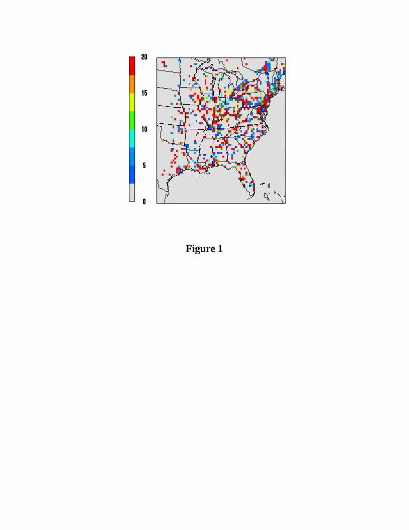
Figure 1

Figure 2

(a)

(b)

(c)0.0

1.0

2.0

3.0

4.0

5.0

6.0

7.0

8.0OCECClSoil

Con

cent

ratio

n (

µg

m-3

)

0.0

20.0

40.0

60.0

80.0

100.0

PM2.5SulfateInorganics

Con

cent

ratio

n (

µg

m-3

)

0.0

5.0

10.0

15.0

20.0

25.0

30.0

7/18 7/22 7/26 7/30 8/3 8/7 8/11 8/15 8/19 8/23

Observation50%100%

SO

42- (

Date (1995)

µg

m-3

)

Beginning Dust Pre-Hurricane

Hurricane Transition Peak Post-peak

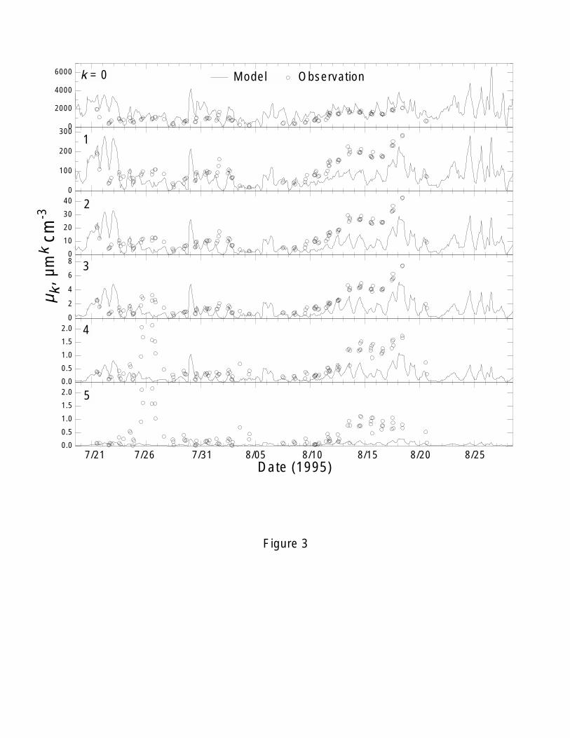
40

30

20

10

0

2

300

200

100

0

1

6000

4000

2000

0

Model Observationk = 0

2.0

1.5

1.0

0.5

0.0

Date (1995)7/21 7/26 7/31 8/05 8/10 8/15 8/20 8/25

5

2.0

1.5

1.0

0.5

0.0

4

8

6

4

2

0

3

µk ,

µmk

cm-3

Figure 3

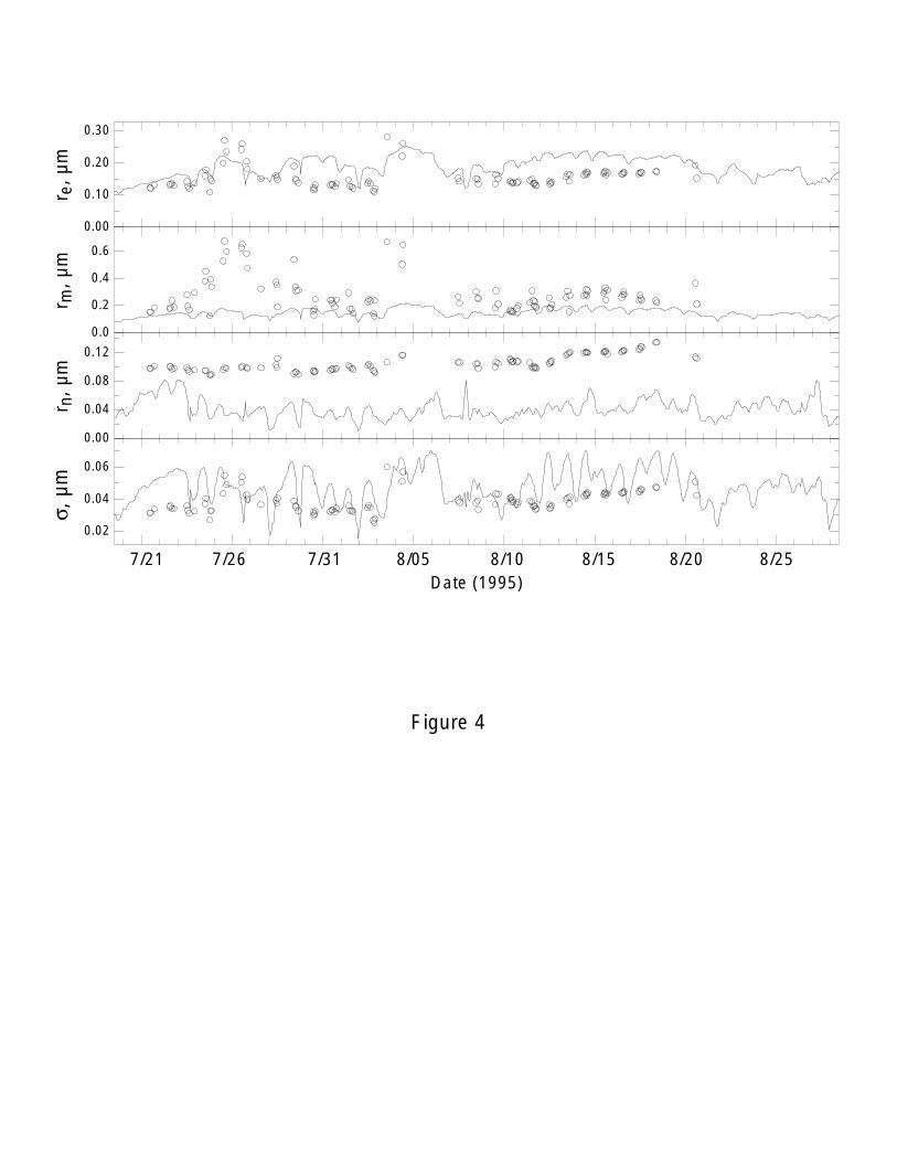
0.12

0.08

0.04

0.00

rn,

µm

0.30

0.20

0.10

0.00

re,

µm

0.6

0.4

0.2

0.0

rm

, µm

0.06

0.04

0.02

σ, µ

m

Date (1995)7/21 7/26 7/31 8/05 8/10 8/15 8/20 8/25

Figure 4

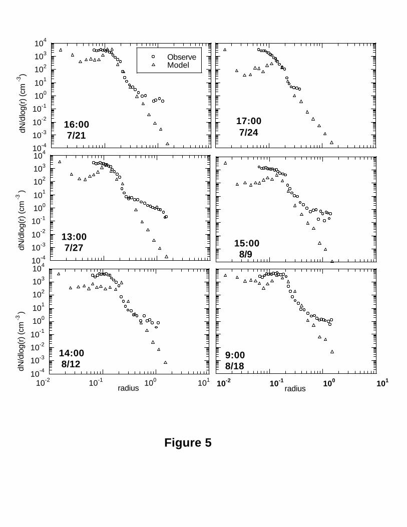
17:007/24

15:008/9

10-2 10-1 100 101

9:008/18

radius

10-4

10-3

10-2

10-1

100

101

102

103

104

16:007/21

ObserveModel

dN/d

log(

r) (c

m -3

)

10-4

10-3

10-2

10-1

100

101

102

103

104

13:007/27dN

/dlo

g(r)

(cm

-3 )

10-4

10-3

10-2

10-1

100

101

102

103

104

10-2 10-1 100 101

14:008/12dN

/dlo

g(r)

(cm

-3

radius

)

Figure 5

40

30

20

10

0

2

300

200

100

0

1

6000

4000

2000

0

Model Observation

k = 0

0.250.200.150.100.050.00

Date (1995)7/21 7/26 7/31 8/05 8/10 8/15 8/20 8/25

5

1.0

0.8

0.6

0.4

0.2

0.0

4

543210

3

µk ,

µmk

cm-3

Figure 6

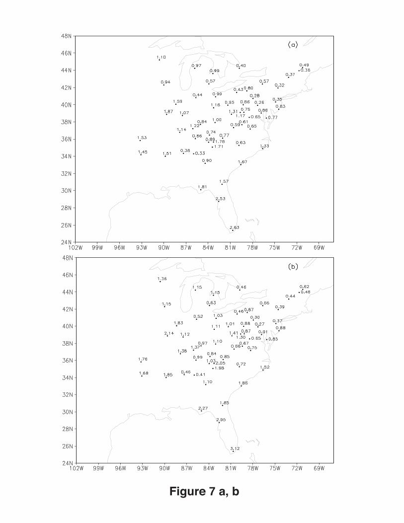
Figure 7 a, b

Figure 7 c, d

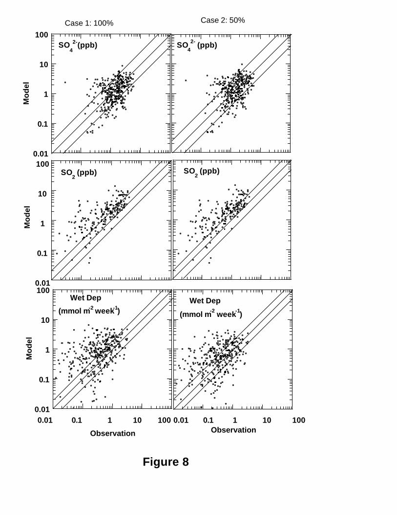
Case 1: 100% Case 2: 50%

Figure 8

0.01

0.1

1

10

100M

od

el

SO4

2-(ppb) SO4

2- (ppb)

0.01

0.1

1

10

100

Mo

del

SO2 (ppb) SO

2 (ppb)

0.01

0.1

1

10

100

0.01 0.1 1 10 100

Mo

del

Observation

Wet Dep

(mmol m-2 week-1)

0.01 0.1 1 10 100Observation

Wet Dep

(mmol m-2 week-1)

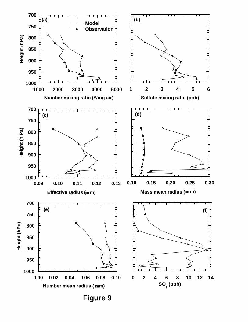
Figure 9

0.00 0.02 0.04 0.06 0.08 0.10

700

750

800

850

900

950

1000

Number mean radius ( µµ m)

(e)

Hei

gh

t (h

Pa)

0.10 0.15 0.20 0.25 0.30

Mass mean radius (µµ m)

(d)

700

750

800

850

900

950

10001000 2000 3000 4000 5000

ModelObservation

Hei

gh

t (h

Pa)

Number mixing ratio (#/mg air)

(a)

1 2 3 4 5 6

Sulfate mixing ratio (ppb)

(b)

700

750

800

850

900

950

10000.09 0.10 0.11 0.12 0.13

Hei

gh

t (h

Pa)

Effective radius (µµ m)

(c)

0 2 4 6 8 10 12 14SO

2 (ppb)

(f)

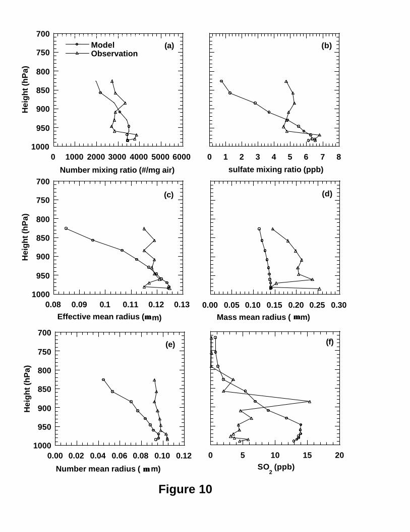
Figure 10

700

750

800

850

900

950

10000.00 0.02 0.04 0.06 0.08 0.10 0.12

Hei

gh

t (h

Pa)

Number mean radius ( µµ m)

(e)

0 5 10 15 20SO

2 (ppb)

(f)

700

750

800

850

900

950

10000 1000 2000 3000 4000 5000 6000

ModelObservation

Hei

gh

t (h

Pa)

Number mixing ratio (#/mg air)

(a)

0 1 2 3 4 5 6 7 8

sulfate mixing ratio (ppb)

(b)

700

750

800

850

900

950

10000.08 0.09 0.1 0.11 0.12 0.13

Hei

gh

t (h

Pa)

Effective mean radius (µµ m)

(c)

0.00 0.05 0.10 0.15 0.20 0.25 0.30

Mass mean radius ( µµ m)

(d)

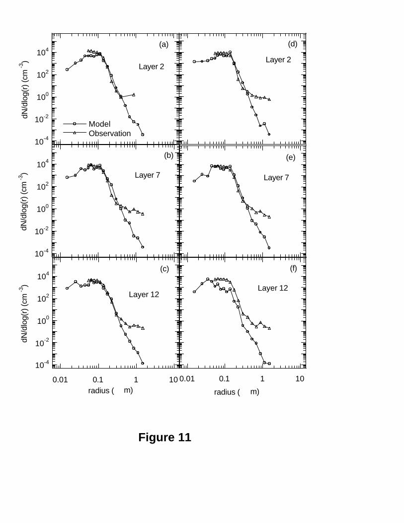
10-4

10-2

100

102

104

ModelObservation

dN/d

log(

r) (c

m-3

)

(a)

Layer 2

10-4

10-2

100

102

104

dN/d

log(

r) (c

m-3

)

(b)

Layer 7

10-4

10-2

100

102

104

0.01 0.1 1 10

dN/d

log(

r) (c

m-3

)

radius ( µ m)

Layer 12

(c)

(d)

Layer 2

(e)

Layer 7

0.01 0.1 1 10

radius ( µ m)

(f)

Layer 12

Figure 11

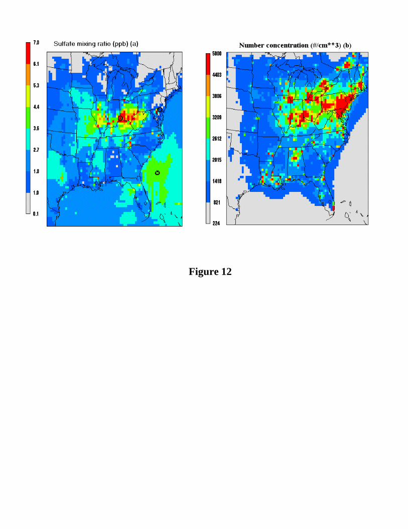
Figure 12

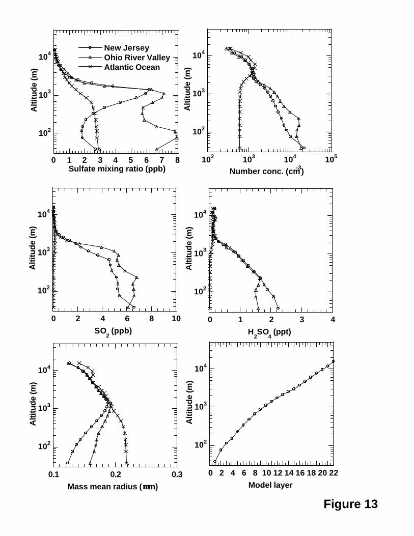
Figure 13

102

103

104

0 1 2 3 4 5 6 7 8

New JerseyOhio River ValleyAtlantic Ocean

Alti

tud

e (m

)

Sulfate mixing ratio (ppb)

102

103

104

102 103 104 105

Alti

tud

e (m

)

Number conc. (cm-3)

102

103

104

0 2 4 6 8 10

Alti

tud

e (m

)

SO2 (ppb)

102

103

104

0 1 2 3 4

Alti

tud

e (m

)

H2SO

4 (ppt)

102

103

104

0.1 0.2 0.3

Alti

tud

e (m

)

Mass mean radius ( m)µµ

102

103

104

0 2 4 6 8 10 12 14 16 18 20 22

Alti

tud

e (m

)

Model layer