1

Molecular Electronic Structure

Millard H. Alexander

CONTENTS

I. Molecular structure 2

A. The Born-Oppenheimer approximation 2

B. The one-electron H+2 ion 4

C. The H2 molecule 9

II. Homonuclear Diatomics: First-Row Elements 12

III. Homonuclear Diatomics: Second-Row Elements 14

A. The diatomic boron molecule 16

1. 1Σ+g state 16

2. 3Σ−g state 19

B. The diatomic oxygen and carbon molecules in their lowest states 20

1. O2 20

2. Reflection symmetry 21

3. Electron repulsion 23

4. MCSCF calculations for O2 24

5. The C2 molecule 25

C. Spectroscopic notation for diatomic molecules 28

D. States of other homonuclear diatomic molecules and ions 28

IV. Near-homonuclear diatomics 29

V. Triatomic Hydrides 31

VI. Rovibronic states of diatomic molecules 39

A. Wavefunctions 39

B. Energies 41

C. Physical interpretation of the spectroscopic expansion coefficients 45

2

I. MOLECULAR STRUCTURE

A. The Born-Oppenheimer approximation

Within the Born-Oppenheimer approximation, the full nuclear-electronic wavefunction

Ψ(~r, ~R), where ~r refers, collectively to the coordinates of all the elecrons and ~R, to the

coordinates of all the nuclei, may be expanded in terms of the electronic wavefunctions at a

fixed ~R, namely

Ψ(~r, ~R) =∑

k

Ck(~R)φ(k)el (~r;

~R)

where

Hel(~r; ~R) φ(k)el (~r;

~R) = E(k))el (~R) φ

(k)el (~r;

~R) (1)

and the electronic Hamiltonian is

Hel(~r; ~R) = −1

2

∑

i

∇2i −

∑

i,j

Zj

rij+∑

i

∑

i′>i

1

ri,i′

Here i and i′ refer to the electrons and j refers to the nuclei.

At each value of the nuclear coordinates ~R one solves the Schroedinger equation (1)

obtaining a complete set of electronic energies and electronic wavefunctions, both of which

depend, parametrically, on ~R. Then, the Born-Oppenheimer approximation states that

the motion of the nuclei is defined by the Ck(~R) expansion coefficients, which satisfy the

Schroedinger equation

HnucCk(~R) = ECk(~R)

where

Hnuc = −1

2

∑

j

∇2j

Mj

+ Ek(el)(

~R) +∑

j

∑

j′>j

ZjZj′

Rjj′

Thus, the potential for the motion of the nuclei is the sum of the electronic energy (which de-

pends on ~R) and the nuclear repulsion. The Born-Oppenheimer approximation is discussed

in more detail in Appendix B.

In the case of a diatomic molecule, we separate out the motion of the center of mass

~R =[

M1~R1 +M2

~R2

]

/ (M1 +M2)

3

from the relative motion

~R = ~R2 − ~R1

Since the electronic energy and the nuclear repulsion depend only on the relative separation

of the two nuclei, not their position in space, the Hamiltonian can be written

Hnuc(~R1, ~R2) = − 1

M1 +M2∇2

R − 1

µ∇2

R + E(k)el (R) + Z1Z2/R

where the reduced mass is defined as µ = M1M2/(M1 +M2). This separation is discussed

in more detail in Appendix F.

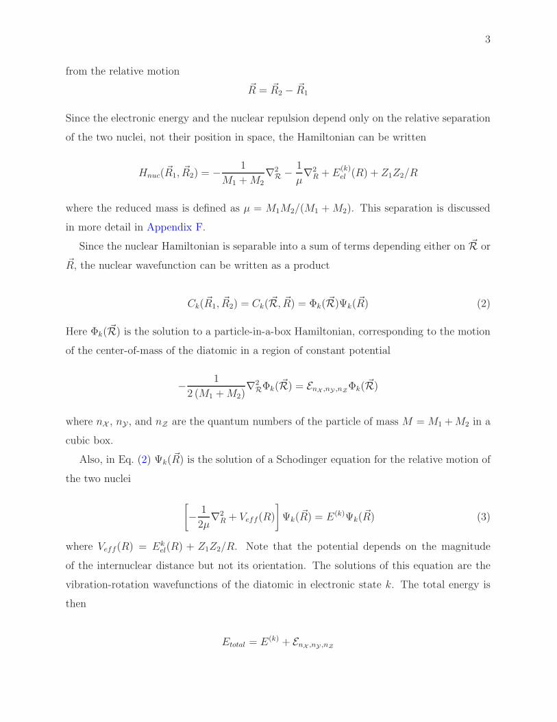
Since the nuclear Hamiltonian is separable into a sum of terms depending either on ~R or

~R, the nuclear wavefunction can be written as a product

Ck(~R1, ~R2) = Ck( ~R, ~R) = Φk( ~R)Ψk(~R) (2)

Here Φk( ~R) is the solution to a particle-in-a-box Hamiltonian, corresponding to the motion

of the center-of-mass of the diatomic in a region of constant potential

− 1

2 (M1 +M2)∇2

RΦk( ~R) = EnX ,nY ,nZΦk( ~R)

where nX , nY , and nZ are the quantum numbers of the particle of mass M =M1 +M2 in a

cubic box.

Also, in Eq. (2) Ψk(~R) is the solution of a Schodinger equation for the relative motion of

the two nuclei

[

− 1

2µ∇2

R + Veff(R)

]

Ψk(~R) = E(k)Ψk(~R) (3)

where Veff(R) = Ekel(R) + Z1Z2/R. Note that the potential depends on the magnitude

of the internuclear distance but not its orientation. The solutions of this equation are the

vibration-rotation wavefunctions of the diatomic in electronic state k. The total energy is

then

Etotal = E(k) + EnX ,nY ,nZ

4

Thus, before one can solve the Schroedinger equation for the motion of the nuclei, one needs

the electronic energy as a function of the internuclear coordinates. Just as in the case of

atoms, in general, one can not solve the electronic Schroedinger equation for more than

one electron. Thus, we need to develop a system of approximations, based on use of the

variational principle. Crucial will be the expansion of molecular electronic wavefunctions

in terms of Slater determinants based on a product of one electron molecular orbitals,

which themselves will be expanded as linear combinations of atomic orbitals. To illustrate

this LCAO-MO method, we start first with the one-electron hydrogen molecular ion (H+2 ),

which has the further advantage that it can be solved exactly.

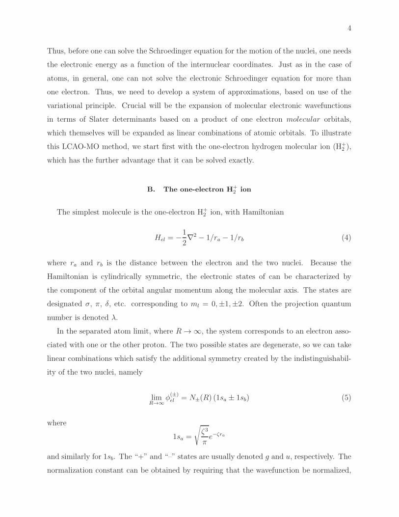
B. The one-electron H+2 ion

The simplest molecule is the one-electron H+2 ion, with Hamiltonian

Hel = −1

2∇2 − 1/ra − 1/rb (4)

where ra and rb is the distance between the electron and the two nuclei. Because the

Hamiltonian is cylindrically symmetric, the electronic states of can be characterized by

the component of the orbital angular momentum along the molecular axis. The states are

designated σ, π, δ, etc. corresponding to ml = 0,±1,±2. Often the projection quantum

number is denoted λ.

In the separated atom limit, where R→ ∞, the system corresponds to an electron asso-

ciated with one or the other proton. The two possible states are degenerate, so we can take

linear combinations which satisfy the additional symmetry created by the indistinguishabil-

ity of the two nuclei, namely

limR→∞

φ(±)el = N±(R) (1sa ± 1sb) (5)

where

1sa =

√

ζ3

πe−ζra

and similarly for 1sb. The “+” and “–” states are usually denoted g and u, respectively. The

normalization constant can be obtained by requiring that the wavefunction be normalized,

5

so that

1 = N2±

∫

φ2el dV

= N2±

∫

[1sa + 1sb]2 dV

= N2±

[∫

1s2adV +∫

1s2bdV + 2∫

1sa1sb dV]

(6)

Since the 1s functions are normalized, we see that the electronic wavefunctions can be

normalized by requiring that

N2±(~r, R) =

[

1

2(1± S(R))

]1/2

(7)

where the overlap is defined as

S(R) =∫

1sa1sb dV

In the united atom limit, where R = 0, the 1sa and 1sb functions coincide, and S = 1, so

that

limR→0

φg(~r) = 1s (8)

as we would expect.

An interesting question is what happens to the u function in the united atom limit (R → 0). You can show

(using the expression for S(R) given on the next page) that

limR→0

φu(R) ≈ cos θ exp(−ζr) +O(R)

where r and θ are the usual spherical polar coordinates with origin at the mid-point of the bond. This has

the correct angular dependence and radial dependence (at large r) of the 2pz atomic orbital of the united

atom, but not the correct dependence on r as small r, since limr→0 2pz ∼ r cos θ exp(−ζr).

The variational energy of the g state is

Eel(R) =1

2(1 + S)[Taa + Tbb + Tab + Tba + Vaaa + Vaab + Vbba + Vbbb + Vaba + Vabb + Vbaa + Vbab]

where

Tmn =∫

1sm

(

−1

2∇)

1smdV

6

and

Vmnk =∫

1sm (−1/rk) 1sndV

Not all the T and V terms are independent. By symmetry, you can show that Taa = Tbb,

Tab = Tba, Vaaa = Vbbb, Vaab = Vbba, and Vaba = Vabb = Vbaa = Vbab. Thus, the expression for

the electronic energy simplifies to

Eel(R) =1

(1 + S)[Taa + Tab + Vaaa + Vaab + 2Vaba]

=1

(1 + S)[Taa + Vaaa + Tab + 2Vaba + Vaab] (9)

The first two terms correspond to the energy of the H atom (calculated with a 1s orbital

with exponent ζ , the second two terms correspond to the energy (kinetic + potential) of

an overlap density 1sa1sb, and the last term, to the attraction between an electron on one

nucleus and the other nucleus.

All these one-electron integrals can be evaluated. We find

S(R) =(

1 + ρ+1

3ρ2)

e−ρ

Vaaa = −ζ

Vaba(R) = −ζ(1 + ρ)e−ρ

Vaab(R) = −ζρ

[

1− (1 + ρ)e−2ρ]

Taa =1

2ζ2

and

Tab = −1

2ζ2(

−1− ρ+1

3ρ2)

e−ρ

where ρ = ζR.

Problem 1 Write a Matlab script to use the expressions immediately above to determine

the electronic energy of H+2 as a function if the internuclear separation R. Check your

expression by knowing that at ρ = 0 (the united atom limit) the energy is minimized when

ζ = 2 (He+ ion) and that at ρ = ∞ (the separated atom limit) the energy is minimized

when ζ = 1 (H atom plus a bare proton). As a further check on your expression, for ζ = 1

7

at R = 2 bohr, the electronic energy is −1.05377 hartree.

Determine the dissociation energy, the equilibrium internuclear separation, and the vi-

brational frequency if the screening constant is held equal to the value appropriate for the

H atom (ζ = 1). Compare these with experiment (see webbook.nist.gov).

Now, at each value of R, you can minimize the energy by varying ζ . Do so, to get the

best potential curve for a wavefunction of the form φ(+)el [Eq. (5)]. Compare the dissociation

energy, equilibrium separation, and vibrational frequency with experiment. Finally, use

the contour command in Matlab to prepare contour plots of the square of the 1σg orbital

of H+2 for internuclear distances of 1, 2, and 4 bohr. The plots should look similar to Fig. 3,

except that the simple 1sa + 1sb expression does not include polarization of the atomic

orbitals.

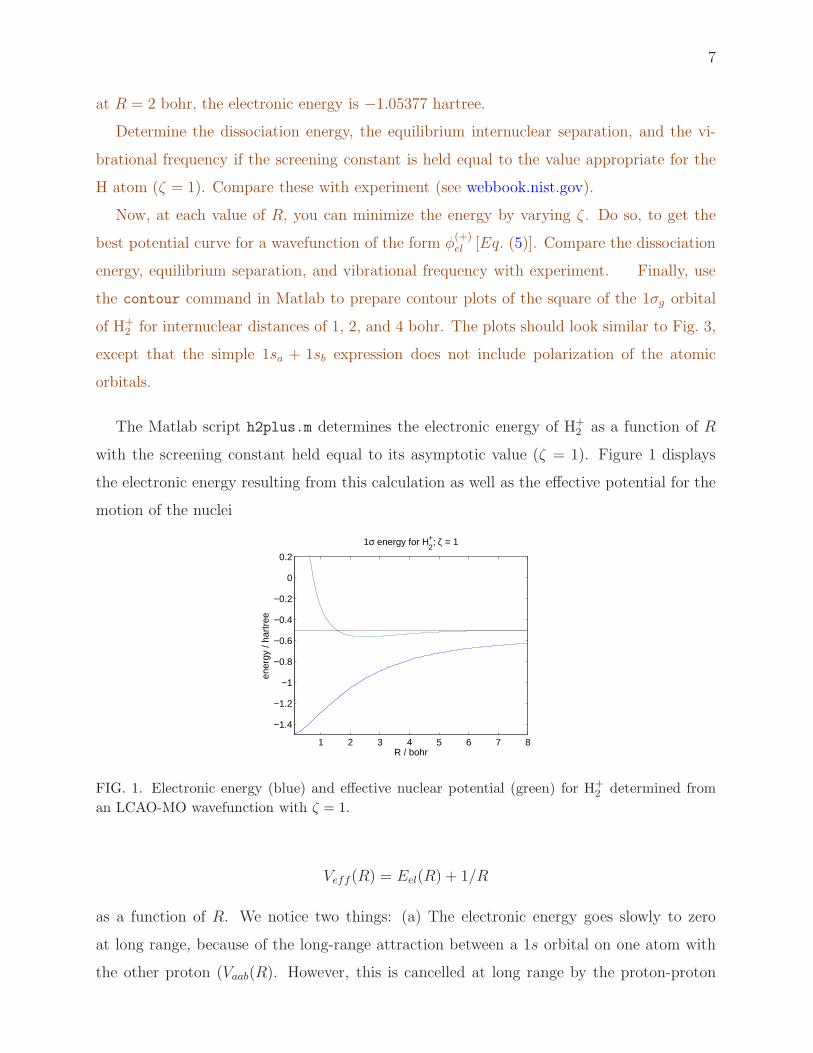
The Matlab script h2plus.m determines the electronic energy of H+2 as a function of R

with the screening constant held equal to its asymptotic value (ζ = 1). Figure 1 displays

the electronic energy resulting from this calculation as well as the effective potential for the

motion of the nuclei

1 2 3 4 5 6 7 8

−1.4

−1.2

−1

−0.8

−0.6

−0.4

−0.2

0

0.2

ener

gy /

hart

ree

R / bohr

1σ energy for H2+; ζ = 1

FIG. 1. Electronic energy (blue) and effective nuclear potential (green) for H+2 determined from

an LCAO-MO wavefunction with ζ = 1.

Veff(R) = Eel(R) + 1/R

as a function of R. We notice two things: (a) The electronic energy goes slowly to zero

at long range, because of the long-range attraction between a 1s orbital on one atom with

the other proton (Vaab(R). However, this is cancelled at long range by the proton-proton

8

repulsion (1/R) so that at long range the effective potential goes rapidly to zero. Also (b)

the depth of the attractive well is quite small in comparison with the large total energies.

For this calculation in which we constrain the orbital exponent ζ to equal 1, the dissociation

energy is calculated to be De = 0.0648 hartree = 1.75 eV and the position of the minimum

is Re = 2.046 bohr.

A better approximation can be obtained by varying allowing the exponent ζ to vary a

function of R to minimize the electronic energy. Then, we you add back 1/R you obtain a

potential which has a dissociation energy of De = 2.35eV at Re = 2.003 bohr.

The true dissociation energy of H+2 is 0.1026 hartree = 2.793 eV with Re = 1.997 bohr.

Why is the simple LCAO-MO wavefunction of Eq. (7) in error? Because we have assumed

that the electron is described by a linear combination of spherical orbitals. In fact, the

presence of the additional proton will polarize the charge distribution, pulling the electron

a bit toward the bare proton. This is shown, schematically, in the next figure

z

HA HB

z

HA HB

unpolarized polarized

FIG. 2. Illustration of the lowest 1σg orbital of H+2 . The left cartoon is the primitive linear

combination of 1s atomic orbitals. The right cartoon shows the effect of polarization of the these

atomic orbitals

We could include the effect of polarization by using a more flexible molecular orbital

description

φg(~r, R) = C1s

[

1

2(1 + S1s)

]1/2

(1sa + 1sb) + C2p

[

1

2(1− S2pz)

]1/2

(2pza − 2pzb) (10)

where C1s and C2p are variable coefficients. Note the minus sign in the second term. Because

of the directionality of the 2pz orbitals, it is the minus linear combination which has g

symmetry. Also, because of this directionality, the overlap S2pz is negative.

9

C. The H2 molecule

The electronic Hamiltonian for the two-electron H2 molecule is

Hel(1, 2) = h(1) + h(2) + 1/r12

where h(1) is the one-electron Hamiltonian of Eq. (4). For atoms, the one-electron 1s ground

state of the H atom provides the logical approximation for the electronic wavefunction of

the two-electron He atom, namely 1s2. If we follow this approach for H2 we would write the

electronic wavefunction as (using Slater determinantal notation)

φel(1, 2) = |1σg1σg| (11)

With this choice of a wavefunction, the variational energy is (similar to the case of the He

atom)

EH2(R) = 2ε1σg

+[

1σ2g

∣

∣

∣ 1σ2g

]

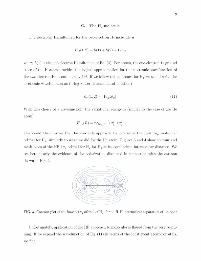
One could then invoke the Hartree-Fock approach to determine the best 1σg molecular

orbital for H2, similarly to what we did for the He atom. Figures 3 and 4 show contour and

mesh plots of the HF 1σg orbital for H2 for H2 at its equilibrium internuclear distance. We

see here clearly the evidence of the polarization discussed in connection with the cartoon

shown in Fig. 2.

H

H

FIG. 3. Contour plot of the lowest 1σg orbital of H2, for an H–H internuclear separation of 1.4 bohr

Unfortunately, application of the HF approach to molecules is flawed from the very begin-

ning. If we expand the wavefunction of Eq. (11) in terms of the constituent atomic orbitals,

we find

10

FIG. 4. Surface mesh plot of the lowest 1σg orbital of H2, for an H–H internuclear separation of

1.4 bohr

φel(1, 2) =1

2(1− S2)[ |1sa1sa|+ |1sb1sb|+ |1sa1sb|+ |1sb1sa| ] (12)

The first two determinants correspond to associating both electrons with the same proton,

which is an ionic electron configuration, either H+H− or H−H+, while the later two deter-

minants correspond to the usual covalent description, where each proton contributes one

electron to the bond. We know that the ground state pathway for dissociation must lead to

the one electron associated with each proton, namely

limR→∞

H2(R) = H + H

or, in other words

limR→∞

φel(1, 2) ≈ [ |1sa1sb|+ |1sb1sa| ]

Thus, a serious flaw of conventional, single-determinant Hartree-Fock calculations on

molecules is the inability of a single-determinant wavefunction to describe correctly the

dissociation of the molecule.

One way of overcoming this deficiency is to use an approximate wavefunction which does

dissociate correctly. This approach was first advocated by Heitler and London. In the HL

or “valence-bond” description the ionic configurations in Eq. (12) are eliminated, leaving

φel(1, 2) =

[

1

2(1 + S2)

]1/2

[ |1sa1sb|+ |1sb1sa| ] (13)

Since the variational method allows us to introduce increasing flexibility into the wave-

11

function, while guaranteeing that the energy will always lie above the true ground state

electronic energy, we could allow a variable mix of ionic and covalent configurations

φel(1, 2) = CI

[

1

2(1 + S2)

]1/2

[ |1sa1sa|+ |1sb1sb| ] + CC

[

1

2(1 + S2)

]1/2

[ |1sa1sb|+ |1sb1sa| ](14)

where CI and CC are variable coefficients which satisfy C2I + C2

C = 1.

Alternatively, we could write the wavefunction as

φel(1, 2) = Cg |1σg1σg|+ Cu |1σu1σu| (15)

where,

limR→∞

1σg(u) =

[

1

2(1± S)

]1/2

(1sa ± 1sb)

Note that although the 1σu orbital is antisymmetric with respect to interchange of the

two nuclei, the product of two antisymmetric functions is symmetric, so that the |1σu1σu|determinant is symmetric, the same as the |1σg1σg| determinant.

Thus, a mix of the two determinants in Eq. (15) will allow correct dissociation of the

H2 molecule. One can imagine an extended SCF procedure in which one starts with the

two-determinant wavefunction of Eq. (15) [this is called a dual-reference (or, in general,

multi-reference) description] and then determines, within a chosen atomic-orbital basis set,

the optimal 1σg and 1σu functions and the coefficients Cg and Cu chosen to minimize the

electronic energy at each value of R. This is the so-called multi-configuration, self-consistent-

field approach (MCSCF).

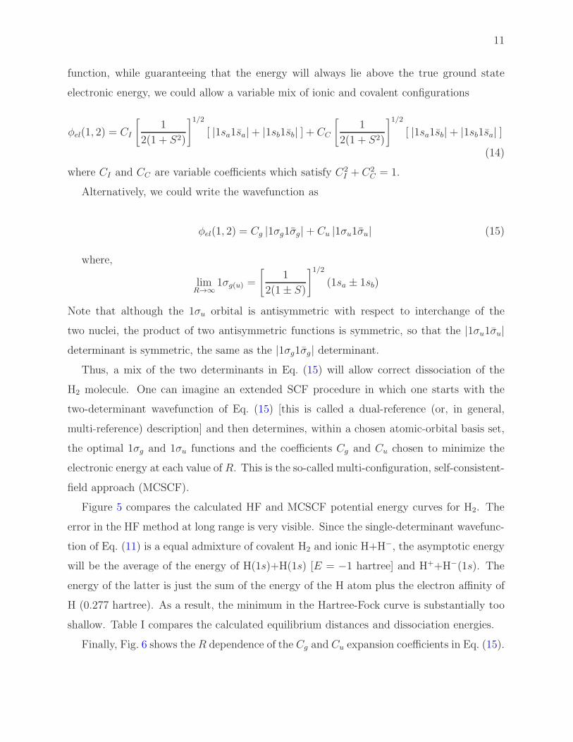
Figure 5 compares the calculated HF and MCSCF potential energy curves for H2. The

error in the HF method at long range is very visible. Since the single-determinant wavefunc-

tion of Eq. (11) is a equal admixture of covalent H2 and ionic H+H−, the asymptotic energy

will be the average of the energy of H(1s)+H(1s) [E = −1 hartree] and H++H−(1s). The

energy of the latter is just the sum of the energy of the H atom plus the electron affinity of

H (0.277 hartree). As a result, the minimum in the Hartree-Fock curve is substantially too

shallow. Table I compares the calculated equilibrium distances and dissociation energies.

Finally, Fig. 6 shows the R dependence of the Cg and Cu expansion coefficients in Eq. (15).

12

0 1 2 3 4 5 6 7 8 9 10

−1.15

−1.1

−1.05

−1

−0.95

−0.9

−0.85

−0.8

−0.75

−0.7

R / bohr

V(R) / Hartree HF

MCSCF

MCSCF+CI

FIG. 5. Calculated potential curves [V (R) = Eel(R) + 1/R] for H2, determined within the single-

reference HF method, the two-configuration MCSCF method, and the two-configuration MCSCF

method with the addition of configuration interaction.

TABLE I. Calculated internuclear separations and dissociation energies for H2.

Method Re (bohr) De (eV)

HFSCF 1.391 3.638

MCSCF 1.430 4.147

MCSCF+CI 1.407 4.748

exacta 1.401 4.747

a W. Kolos and L. Wolniewicz, “Potential-Energy Curves for the X1Σ+g , b

3Σ+u , and C1Πu States of the

Hydrogen Molecule,” J. Chem. Phys. 43, 2429 (1965).

II. HOMONUCLEAR DIATOMICS: FIRST-ROW ELEMENTS

Despite its deficiencies the single-configuration description does provide an excellent de-

scription of the electronic wave function for small molecules. As we have seen, the bonding

1σg orbital is singly occupied in H+2 , but doubly occupied in the H2 molecule. We would then

expect naively that the bond in H2 would be twice as strong a in the case of the H+2 ion. A

stronger bond corresponds to a deeper well in the potential V (R). The vibrational motion

of a diatomic can be approximated as harmonic motion about the minimum in V (R), with

a force constant given by

k =∂2V (R)

∂R2

∣

∣

∣

∣

∣

R=Re

13

0 1 2 3 4 5 6 7 8 9 100

0.1

0.2

0.3

0.4

0.5

0.6

0.7

0.8

0.9

1

R / bohr

abs(

C)

FIG. 6. Calculated coefficients Cg (blue) and Cu (green) in the two-configuration MCSCF approx-

imation to the H2 electronic wavefunction. The absolute values of the coefficients are shown. The

sign of Cu is opposite to that of the sign of Cg.

The vibrational frequency is then

ω =√

k/µ

The spacing between adjacent vibrational levels is hω. Spectroscopists tend to designate

this spacing as ωe in wavenumber units. This value corresponds to 1/λ, where λ is the

wavelength of light which corresponds to the vibrational spacing. Thus

ωe = 1/λ =1

2πc

√

kµ

As we have seen, the dissociation energy of H2 is indeed larger than that of H+2 , as shown

in Table [? ].

Chemists often describe the strength of a bond in terms of the “bond-order” which is the

one-half the total number of electrons in bonding molecular orbitals minus the number of

electrons in antibonding molecular orbitals, namely

bo =1

2(nbonding − nantibonding) (16)

The depth of the well in V (R) is called De (usually defined as a positive number), which

is a measure of the strength of the bond. Since the lowest vibrational level of a diatomic

molecule – the zero-point energy – is hω/2, the experimentally-measurable binding energy

14

is less than De. This is called D0, namely

D0 = De − ωe/2

.

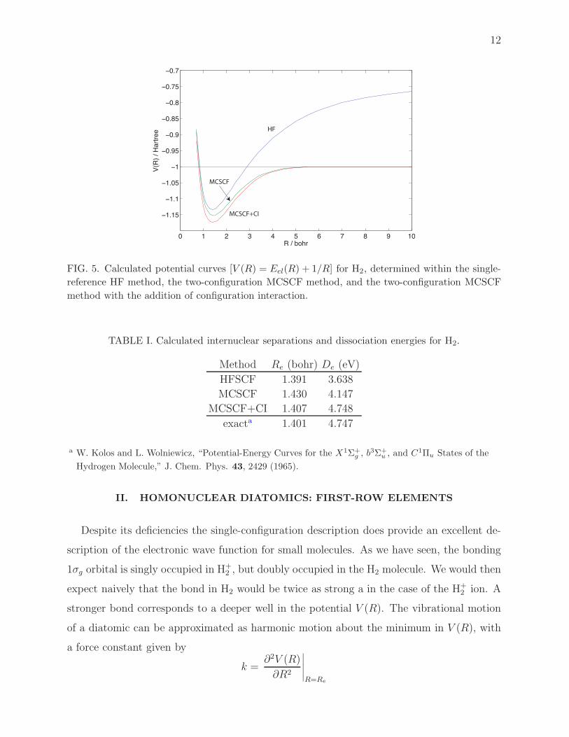
Table II lists the values of ωe, D0, and Re for the homonuclear diatomic molecules and ions

that can be formed out of the first-row atoms. We observe that the bond energy correlates

very well with the bond order. However, going from a bond order of 1/2 to 1 doesn’t quite

double the binding energy.

TABLE II. States, dominant electronic configurations, and spectroscopic constants for several first-

row homonuclear diatomic molecules and ions.

System Configuration bob ωea,c D0

d Reb,e

H+2 1σ1

g 0.5 f 2321 2.651 1.052

H2 1σ2g 1 4401 4.4781 0.7414

He+2 1σ2g1σ

1u 0.5 1698 2.365 1.116

He2 1σ2g1σ

2u 0 0 0.090f 2.97f

.

a Bond order, see Eq. (16).b Data from http://webbook.nist.gov.c In wavenumbers.d The dissociation energy out of the lowest vibrational level, in eV, data from K. P. Huber and G.

Herzberg, Molecular Spectra and Molecular Structure. IV. Constants of Diatomic Molecules (Van

Nostrand Reinhold, New York, 1979)e Distance in A.f The He2 molecule shows only a very small van der Walls well at large distance.

III. HOMONUCLEAR DIATOMICS: SECOND-ROW ELEMENTS

Despite the deficiencies of the single-configuration description, the electronic wavefunc-

tions of the larger homonuclear diatomics are built up by assigning electrons to the lin-

ear combination of the molecular orbitals built up out of the g and u linear combinations

of the orbitals of the atoms. In order of increasing energy, these are listed in Table II.

15

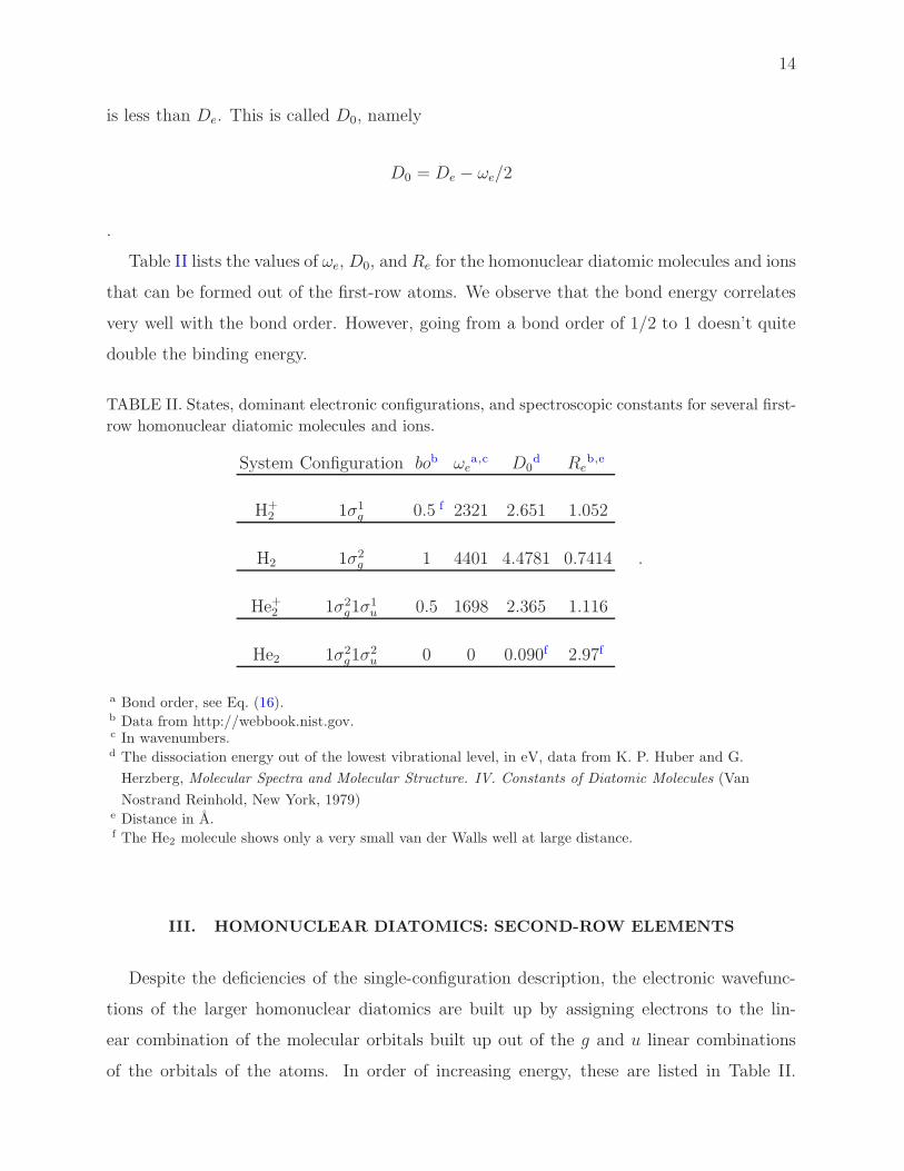
There are three possible linear combinations of 2p atomic orbitals: 2pa,ml=0 ± 2pb,ml=0 and

TABLE III. Molecular orbitals for homonuclear diatomics

MO LCAO description b/aa

1σg 1sa + 1sb b

1σu 1sa − 1sb a

2σg 2sa + 2sb b

2σu 2sa − 2sb a

3σg 2pza − 2pzb b

1πub 2pxa + 2pxb b

1πgb 2pxa − 2pxb a

3σu 2pza − 2pzb a

a Each linear combination should be normalized by multiplying by (1 ± S)−1/2 where S is the overlap

between the constituent atomic orbitals. The orbitals are described as “bonding” (b) or “antibonding”

(a) depending on whether they introduce a buildup of electron probability or a node between the nuclei.b The π orbitals are doubly degenerate.

2pa,ml=±1 ± 2pb,ml=±1 In the first case, the atomic and molecular orbitals are cylindrically

symmetric with respect to the molecular axis, hence they are labelled σ. In the second case

the projection of the electronic orbital angular momentum along the molecular axis is ±1, so

the molecular orbitals are designated π. Note that the g and u label describes the behavior

of the orbital under inversion of the electronic coordinates x→ −x, y → −y, z → −z. Thecorrespondence between the g and u labels and the + or – signs in the description of the

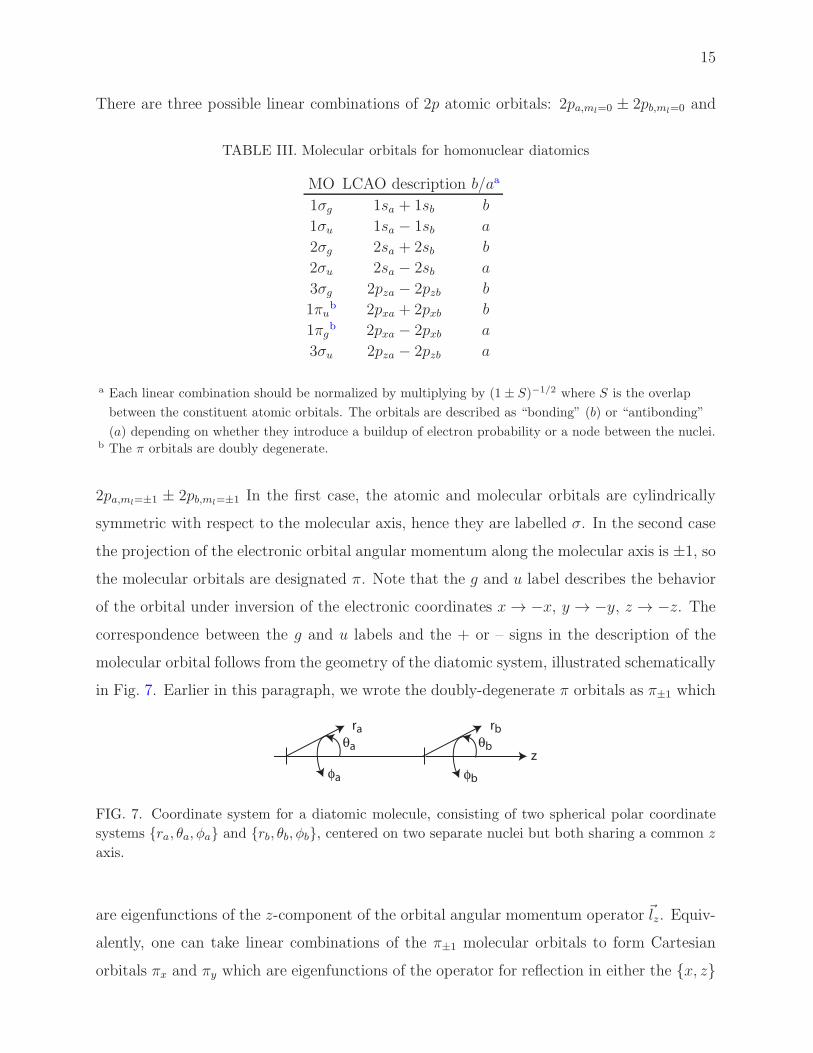
molecular orbital follows from the geometry of the diatomic system, illustrated schematically

in Fig. 7. Earlier in this paragraph, we wrote the doubly-degenerate π orbitals as π±1 which

zθa θb

φa φb

rbra

FIG. 7. Coordinate system for a diatomic molecule, consisting of two spherical polar coordinate

systems {ra, θa, φa} and {rb, θb, φb}, centered on two separate nuclei but both sharing a common z

axis.

are eigenfunctions of the z-component of the orbital angular momentum operator ~lz. Equiv-

alently, one can take linear combinations of the π±1 molecular orbitals to form Cartesian

orbitals πx and πy which are eigenfunctions of the operator for reflection in either the {x, z}

16

or the {y, z} plane.

A. The diatomic boron molecule

1. 1Σ+g state

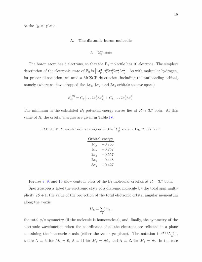
The boron atom has 5 electrons, so that the B2 molecule has 10 electrons. The simplest

description of the electronic state of B2 is∣

∣

∣1σ2g1σ

2u2σ

2g2σ

2u3σ

2g

∣

∣

∣. As with molecular hydrogen,

for proper dissociation, we need a MCSCF description, including the antibonding orbital,

namely (where we have dropped the 1σg, 1σu, and 2σg orbitals to save space)

φ(B)el = Cg

∣

∣

∣. . . 2σ2u3σ

2g

∣

∣

∣+ Cu

∣

∣

∣. . . 2σ2u3σ

2u

∣

∣

∣

The minimum in the calculated B2 potential energy curves lies at R ≈ 3.7 bohr. At this

value of R, the orbital energies are given in Table IV.

TABLE IV. Molecular orbital energies for the 1Σ+g state of B2, R=3.7 bohr.

Orbital energy

1σg −0.763

1σu −0.757

2σg −0.557

2σu −0.448

3σg −0.427

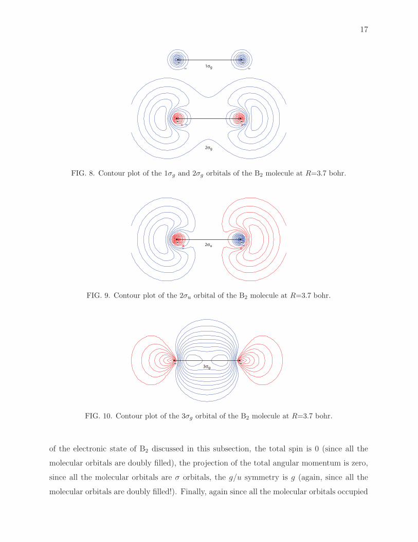
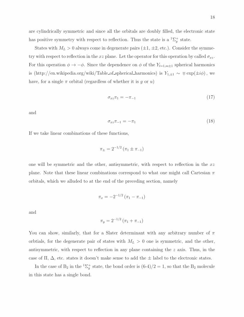
Figures 8, 9, and 10 show contour plots of the B2 molecular orbitals at R = 3.7 bohr.

Spectroscopists label the electronic state of a diatomic molecule by the total spin multi-

plicity 2S + 1, the value of the projection of the total electronic orbital angular momentum

along the z-axis

ML =∑

i

mli ,

the total g/u symmetry (if the molecule is homonuclear), and, finally, the symmetry of the

electronic wavefunction when the coordinates of all the electrons are reflected in a plane

containing the internuclear axis (either the xz or yz plane). The notation is 2S+1Λ+/−g/u ,

where Λ ≡ Σ for Mz = 0, Λ ≡ Π for Mz = ±1, and Λ ≡ ∆ for Mz = ±. In the case

17

2 2 14

14

B

B

2 2

B

B

1σg

2σg

FIG. 8. Contour plot of the 1σg and 2σg orbitals of the B2 molecule at R=3.7 bohr.

2

21

8

18

B

B

2σu

FIG. 9. Contour plot of the 2σu orbital of the B2 molecule at R=3.7 bohr.

B

B

3σg

FIG. 10. Contour plot of the 3σg orbital of the B2 molecule at R=3.7 bohr.

of the electronic state of B2 discussed in this subsection, the total spin is 0 (since all the

molecular orbitals are doubly filled), the projection of the total angular momentum is zero,

since all the molecular orbitals are σ orbitals, the g/u symmetry is g (again, since all the

molecular orbitals are doubly filled!). Finally, again since all the molecular orbitals occupied

18

are cylindrically symmetric and since all the orbitals are doubly filled, the electronic state

has positive symmetry with respect to reflection. Thus the state is a 1Σ+g state.

States withML > 0 always come in degenerate pairs (±1, ±2, etc.). Consider the symme-

try with respect to reflection in the xz plane. Let the operator for this operation by called σxz.

For this operation φ → −φ. Since the dependence on φ of the Yl=1,m±1 spherical harmonics

is (http://en.wikipedia.org/wiki/Table of spherical harmonics) is Y1,±1 ∼ ∓ exp(±iφ) , wehave, for a single π orbital (regardless of whether it is g or u)

σxzπ1 = −π−1 (17)

and

σxzπ−1 = −π1 (18)

If we take linear combinations of these functions,

π± = 2−1/2 (π1 ± π−1)

one will be symmetric and the other, antisymmetric, with respect to reflection in the xz

plane. Note that these linear combinations correspond to what one might call Cartesian π

orbitals, which we alluded to at the end of the preceding section, namely

πx = −2−1/2 (π1 − π−1)

and

πy = 2−1/2 (π1 + π−1)

You can show, similarly, that for a Slater determinant with any arbitrary number of π

orbtials, for the degenerate pair of states with ML > 0 one is symmetric, and the other,

antisymmetric, with respect to reflection in any plane containing the z axis. Thus, in the

case of Π, ∆, etc. states it doesn’t make sense to add the ± label to the electronic states.

In the case of B2 in the 1Σ+g state, the bond order is (6-4)/2 = 1, so that the B2 molecule

in this state has a single bond.

19

2. 3Σ−g state

What makes chemistry interesting is that it is difficult to predict the relative energy

spacing of the lowest states of molecules, except when all the shells are filled. As an exam-

ple, suppose we consider that state of the B2 molecule with electron occupancy (electronic

configuration) . . . 2σ2u1π

2u. Because there are two degenerate 1πu orbitals, one can construct

various different states. Suppose, we put the two outer electrons one in the 1πu,1 and the

other in the 1πu,−1 orbital. One possible Slater determinantal wavefunction for this state is

∣

∣

∣

3Σg

⟩

= |. . . 1πu11πu,−1| (19)

here we have explicitly described only the two electrons in the 1πu molecular orbital. We

use the notation 3ΣMS, where MS is the total projection quantum numbers of the electronic

spin angular momenta. Here, we have MS = 1. We could generate the Slater determinants

for the two states with MS = 0 and MS = −1 by applying the spin lowering operator

S− = s1− + s2−.

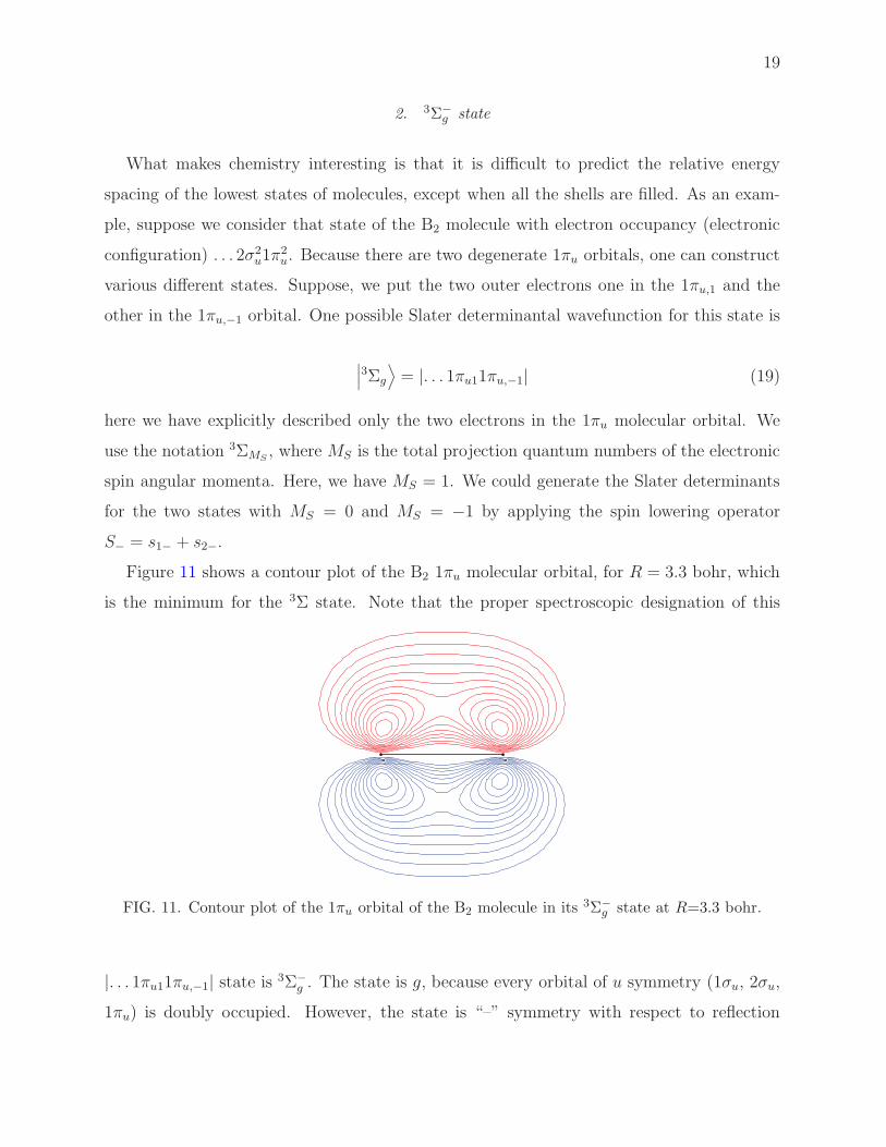
Figure 11 shows a contour plot of the B2 1πu molecular orbital, for R = 3.3 bohr, which

is the minimum for the 3Σ state. Note that the proper spectroscopic designation of this

B

B

FIG. 11. Contour plot of the 1πu orbital of the B2 molecule in its 3Σ−g state at R=3.3 bohr.

|. . . 1πu11πu,−1| state is 3Σ−g . The state is g, because every orbital of u symmetry (1σu, 2σu,

1πu) is doubly occupied. However, the state is “–” symmetry with respect to reflection

20

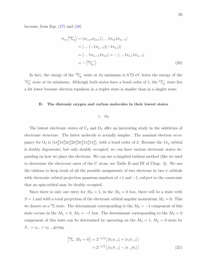
because, from Eqs. (17) and (18)

σxz∣

∣

∣

3Σg

⟩

= (σ1,xzσ2,xz) |. . . 1πu11πu,−1|

= |. . . (−1πu,−1)(−1πu,1)|

= |. . . 1πu,−11πu,1| = − |. . . 1πu,11πu,−1|

= −∣

∣

∣

3Σ−g

⟩

(20)

In fact, the energy of the 3Σ−g state at its minimum is 0.73 eV below the energy of the

1Σ+g state at its minimum. Although both states have a bond order of 1, the 3Σ−

g state lies

a bit lower because electron repulsion in a triplet state is smaller than in a singlet state.

B. The diatomic oxygen and carbon molecules in their lowest states

1. O2

The lowest electronic states of C2 and O2 offer an interesting study in the subtleties of

electronic structure. The latter molecule is actually simpler. The nominal electron occu-

pancy for O2 is |1σ2g1σ

2u2σ

2g2σ

2u3σ

2g1π

4u1π

2g |, with a bond order of 2. Because the 1πg orbital

is doubly degenerate, but only doubly occupied, we can have various electronic states de-

pending on how we place the electrons. We can use a simplied tableau method (like we used

to determine the electronic sates of the C atom; see Table II and III of Chap. 3). We use

the tableau to keep track of all the possible assignments of two electrons in two π orbitals

with electronic orbital projection quantum numbers of +1 and −1, subject to the constraint

that no spin-orbital may be doubly occupied.

Since there is only one entry for MS = 1, in the ML = 0 box, there will be a state with

S = 1 and with a total projection of the electronic orbital angular momentum ML = 0. This

we denote as a 3Σ state. The determinant corresponding to theMS = −1 component of this

state occurs in the ML = 0, MS = −1 box. The determinant corresponding to the MS = 0

component of this state can be determined by operating on the MS = 1, ML = 0 state by

S− = s1− + s2−, giving

∣

∣

∣

3Σ, MS = 0⟩

= 2−1/2 [ |π1π−1|+ |π1π−1| ]

= 2−1/2 [ |π1π−1| − |π−1π1| ] (21)

21

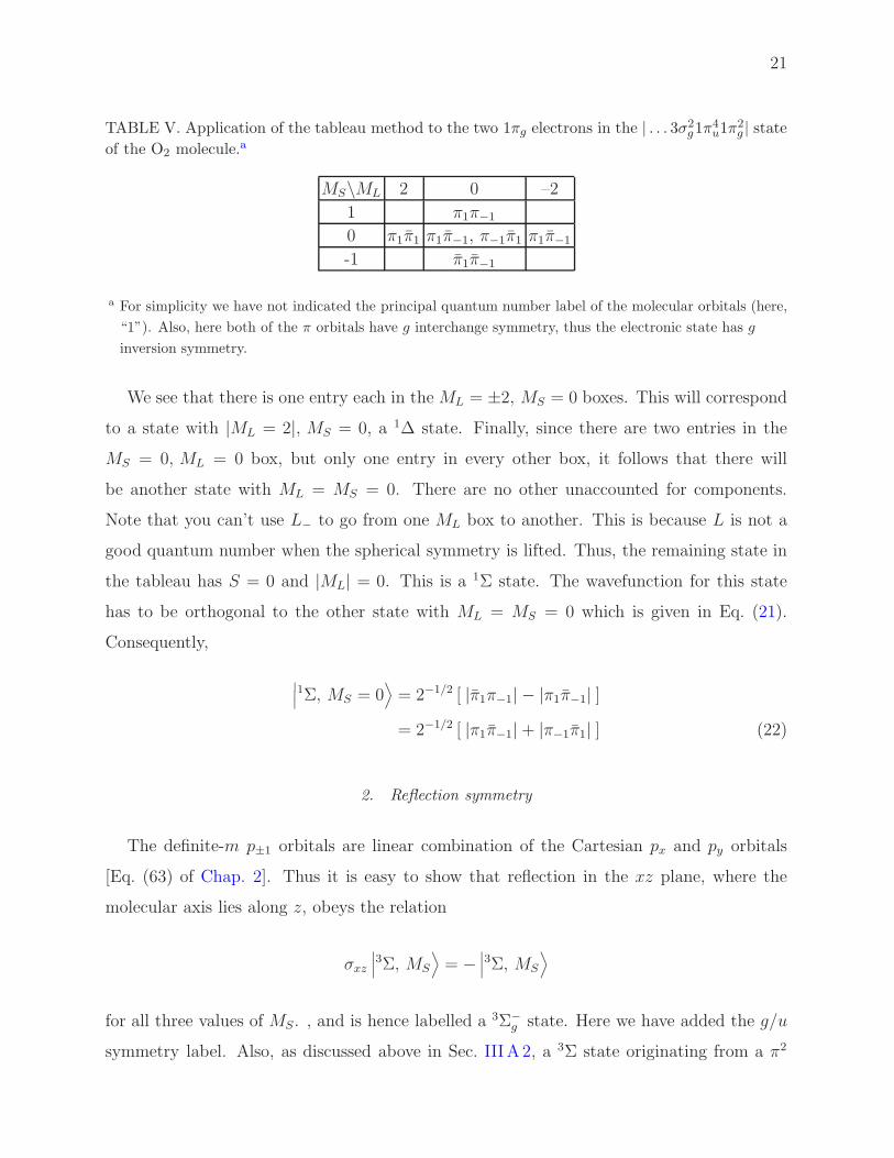
TABLE V. Application of the tableau method to the two 1πg electrons in the | . . . 3σ2g1π

4u1π

2g | state

of the O2 molecule.a

MS\ML 2 0 –2

1 π1π−1

0 π1π1 π1π−1, π−1π1 π1π−1

-1 π1π−1

a For simplicity we have not indicated the principal quantum number label of the molecular orbitals (here,

“1”). Also, here both of the π orbitals have g interchange symmetry, thus the electronic state has g

inversion symmetry.

We see that there is one entry each in theML = ±2, MS = 0 boxes. This will correspond

to a state with |ML = 2|, MS = 0, a 1∆ state. Finally, since there are two entries in the

MS = 0, ML = 0 box, but only one entry in every other box, it follows that there will

be another state with ML = MS = 0. There are no other unaccounted for components.

Note that you can’t use L− to go from one ML box to another. This is because L is not a

good quantum number when the spherical symmetry is lifted. Thus, the remaining state in

the tableau has S = 0 and |ML| = 0. This is a 1Σ state. The wavefunction for this state

has to be orthogonal to the other state with ML = MS = 0 which is given in Eq. (21).

Consequently,

∣

∣

∣

1Σ, MS = 0⟩

= 2−1/2 [ |π1π−1| − |π1π−1| ]

= 2−1/2 [ |π1π−1|+ |π−1π1| ] (22)

2. Reflection symmetry

The definite-m p±1 orbitals are linear combination of the Cartesian px and py orbitals

[Eq. (63) of Chap. 2]. Thus it is easy to show that reflection in the xz plane, where the

molecular axis lies along z, obeys the relation

σxz∣

∣

∣

3Σ, MS

⟩

= −∣

∣

∣

3Σ, MS

⟩

for all three values of MS. , and is hence labelled a 3Σ−g state. Here we have added the g/u

symmetry label. Also, as discussed above in Sec. IIIA 2, a 3Σ state originating from a π2

22

electron occupancy has “–” reflection symmetry. Similarly, the 1Σ state has “+” reflection

symmetry – a 1Σ+g state.

The two components of the ∆ state have the reflection symmetry

σxz∣

∣

∣

1∆ML=±1

⟩

=∣

∣

∣

1∆ML=∓1

⟩

Thus we can take linear combinations of the two definite-m 1∆ states to give two states of

definite reflection symmetry

∣

∣

∣

1∆+g

⟩

= 2−1/2 [ |πxπx| − |πyπy| ]

and∣

∣

∣

1∆−g

⟩

= 2−1/2 [ |πxπy|+ |πyπx| ]

These states are also labelled ∆x2−y2 and ∆xy, for obvious reasons. In general, there exist

both a “–” and “+” component for each state with |ML| 6= 0. Hence, the ± reflection

symmetry label is added only to states of Σ cylindrical symmetry.

It is easy to show that for all three MS components of the 3Σ state

σxz∣

∣

∣

3ΣMS = 1, 0,−1⟩

= −∣

∣

∣

3ΣMS = 1, 0,−1⟩

Hence, the 3Σ state has “–” reflection symmetry. In terms of Cartesian orbitals, the wave-

functions for the three components of the 3Σ state are

∣

∣

∣

3Σ, MS = 1⟩

= |πxπy|

∣

∣

∣

3Σ, MS = −1⟩

= |πxπy|∣

∣

∣

3Σ, MS = 0⟩

= 2−1/2 [ |πxπy| − |πyπx| ]

Similarly, you can show that the reflection symmetry of the 1Σ state, whose wavefunction

is given in Eq. (22), is

σxz∣

∣

∣

1Σ, MS = 0⟩

=∣

∣

∣

1Σ, MS = 0⟩

23

In terms of Cartesian orbitals, the wavefunction for the 1Σ+g state is

∣

∣

∣

1Σ+g

⟩

= 2−1/2 [ |πxπx|+ |πyπy| ]

3. Electron repulsion

Just as in our study of the carbon atom, the splitting between the electronic energy of

the valence states of O2 is governed by the differences in the average value of the electron

repulsion in these states. We need concentrate only on the partially filled 1πg subshell, since

everything else is doubly occupied, independently of how the 1πg subshell is filled. Following

our analysis in Chap. 3 and using the results in Appendix A for expectation values of two-

electron operators between Slater determinantal wavefunctions, we find that the average

value of 1/r12 between the two πg electrons in O2 is

〈1/r12〉3Σ−g=[

π2x

∣

∣

∣ π2y

]

− [πxπy| πyπx]

〈1/r12〉1Σ+g=[

π2x

∣

∣

∣ π2x

]

+ [πxπy| πyπx]

〈1/r12〉1∆+g=[

π2x

∣

∣

∣ π2x

]

− [πxπy| πyπx]

and

〈1/r12〉1∆−g=[

π2x

∣

∣

∣ π2y

]

+ [πxπy| πyπx]

Since the energies of the two components of the 1∆ states must be identical, equating the

last two equations gives

[

π2x

∣

∣

∣ π2x

]

=[

π2x

∣

∣

∣ π2y

]

+ 2 [πxπy| πyπx]

Thus, the 3Σ− state will lie lowest in energy. The 1∆ state will lie above, separated by

twice the exchange integral [πxπy| πyπx]. Finally, the 1Σ+ state will lie above the 1∆ state,

separated by, again, twice the exchange integral. The predicted splitting is then, in units of

this exchange integral, 1∆g −3 Σ−g = 1 and 1Σ+

g −1 ∆g = 1.

24

4. MCSCF calculations for O2

Because the wavefunction for the 1Σ state can’t be represented by a single determinant,

it is not possible to carry out a conventional HF-SCF calculation for all three states of O2.

However, it is possible to carry out an MCSCF calculation in which we include both the

three bonding (3σg, 1πux, and 1πuy) as well as the three antibonding (3σu, 1πgx, and 1πgy)

orbitals. The resulting potential curves are shown in in the left panel of Fig. 12. We see

2 2.5 3 3.50

0.05

0.1

0.15

R / bohr

En

erg

y / h

art

ree

1Σg+

1∆g3Σg

–

2 2.5 3 3.5R / bohr

MCSCF MCSCF+CI

FIG. 12. Electronic potential curves for O2 determined with complete-active-space (CAS) SCF

calculations (left panel) and with CASSCF+CI calculations (right panel).

that the anticipated 3Σ−g <

1 ∆g <1 Σ+

g ordering is found.

The spacing is not quite the identical spacing predicted in the preceding subsection. This

is likely a consequence of the slightly better description, in any approximate calculation,

of the triplet state, because the electrons are automatically kept away from each other in

a triplet state. By carrying out a configuration-interaction calculation after the CAS-SCF

step, we can describe better the so-called “dynamical” correlation. The right panel of Fig. 12

shows the potential curves predicted by CAS-SCF-CI calculations with a larger basis set.

We see that the relative spacing of the three curves come closer to the predicted 1:1 ratio.

Because the first electronic excitation in O2 will involve excitation of an electron from

the antibonding 1πg orbital to the 3σu orbital, which lies significantly higher in energy, there

will likely be no excited states of O2 except deep into the ultraviolet. The transition between

the 1∆g and1Σ+

g states occurs in the green region of the spectrum, but this transition is not

dipole allowed and is hence very week.

25

5. The C2 molecule

The situation in the C2 molecule is more complicated. There are 12 electrons. Once the

1σg, 1σu, 2σg, and 2σu orbitals are filled, that leaves 4 electrons to distribute among the

3 bonding molecular orbitals 3σg, 1πux and 1πuy. One possible assignment is | . . . 3σ2g1π

2u|,

which will give rise to the same 1Σ+g ,

1∆ and 3Σ−g states as in the case of O2. Another

assignment is | . . . 3σ1gπ

3u|. This will give rise to singlet and triplet Πu states. These Π states

have odd (“u”) inversion symmetry because the 1πu orbital is triply filled. In addition, there

is the third possible assignment | . . . 3σ0gπ

4u|. This will give rise to only a 1Σ+

g state.

Problem 2 Follow the discussion in subsubsection IIIB 1, and use the tableau method to

determine Slater determinantal wavefunctions for the allowed states of C2 with electron

occupancy | . . . 3σ2g1π

2u|, | . . . 3σ1

g1π3u|, and | . . . 3σ0

g1π4u|. In each case, label the wavefunction

by the multiplicity 2S + 1, and the value of Λ (Σ,Π,∆) as well as the g/u symmetry.

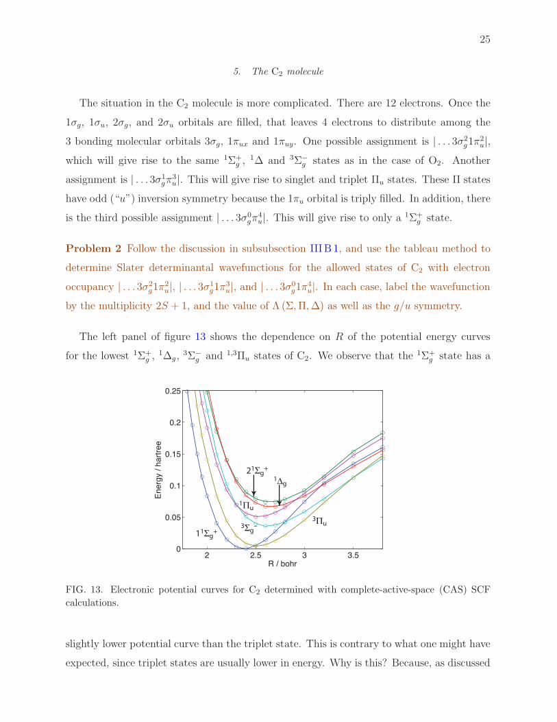
The left panel of figure 13 shows the dependence on R of the potential energy curves

for the lowest 1Σ+g ,

1∆g,3Σ−

g and 1,3Πu states of C2. We observe that the 1Σ+g state has a

2 2.5 3 3.50

0.05

0.1

0.15

0.2

0.25

R / bohr

En

erg

y / h

art

ree

11Σg+

1∆g

3Σg–

3Πu

1Πu

21Σg+

FIG. 13. Electronic potential curves for C2 determined with complete-active-space (CAS) SCF

calculations.

slightly lower potential curve than the triplet state. This is contrary to what one might have

expected, since triplet states are usually lower in energy. Why is this? Because, as discussed

26

above, here there is an additional electronic occupancy possible only for a 1Σ state, namely

| . . . 2σ2u3σ

0gπ

4u|. In addition, there is a third possible electron occupancy which involves

promoting the antibonding 2σu orbital, namely | . . . 2σ0u3σ

2g1π

4u|, which has a bond order

of 3. Both of these electron occupancies are not possible for a state with triplet multiplicity

or with Λ 6= 0. The additional flexibility introduced by these two additional configurations

help lower the energy of the 1Σ+g . state. We can write the wavefunction of the 1Σ+

g state of

C2 as

∣

∣

∣

1Σ+g

⟩

= C1

∣

∣

∣. . . 2σ2g2σ

2u3σ

0g1π

4u

∣

∣

∣+ C2

∣

∣

∣. . . 2σ2g2σ

0u3σ

2g1π

4u

∣

∣

∣

+C32−1/2

[∣

∣

∣. . . 2σ2g2σ

2u3σ

2g1π

2ux

∣

∣

∣+∣

∣

∣. . . 2σ2g2σ

2u3σ

2g1π

2uy

∣

∣

∣

]

+ . . . (23)

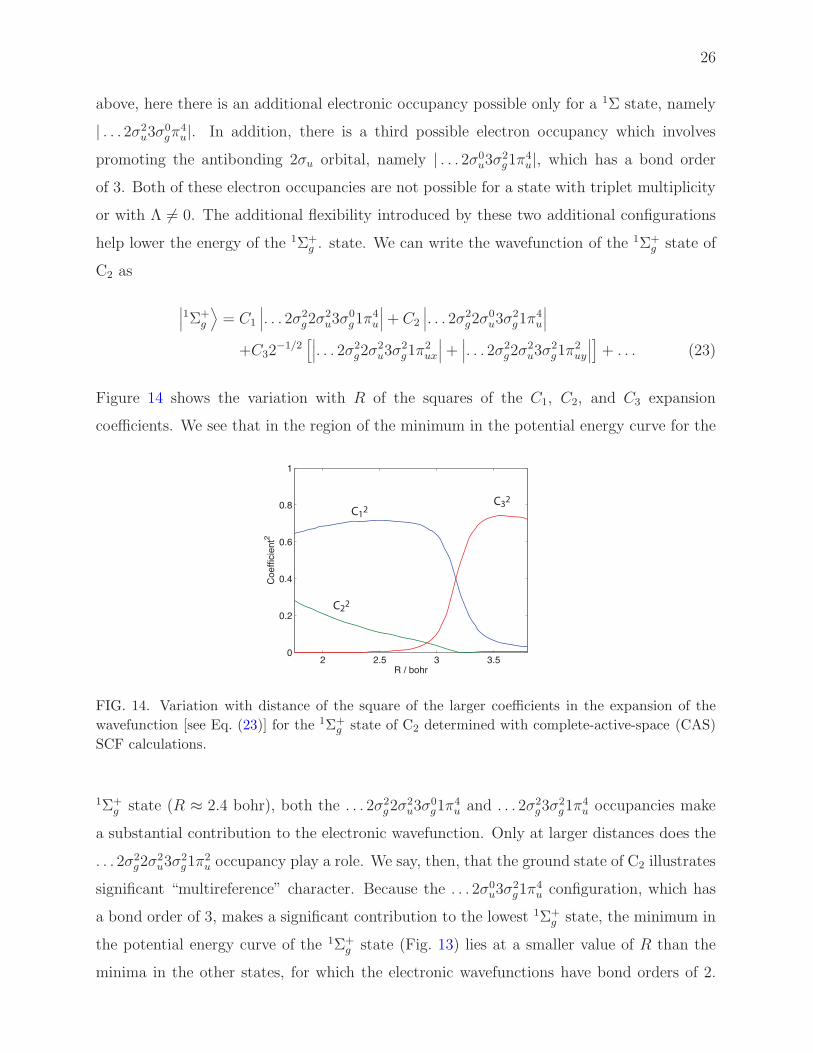
Figure 14 shows the variation with R of the squares of the C1, C2, and C3 expansion

coefficients. We see that in the region of the minimum in the potential energy curve for the

2 2.5 3 3.50

0.2

0.4

0.6

0.8

1

R / bohr

Co

effic

ien

t2

C12

C22

C32

FIG. 14. Variation with distance of the square of the larger coefficients in the expansion of the

wavefunction [see Eq. (23)] for the 1Σ+g state of C2 determined with complete-active-space (CAS)

SCF calculations.

1Σ+g state (R ≈ 2.4 bohr), both the . . . 2σ2

g2σ2u3σ

0g1π

4u and . . . 2σ2

g3σ2g1π

4u occupancies make

a substantial contribution to the electronic wavefunction. Only at larger distances does the

. . . 2σ2g2σ

2u3σ

2g1π

2u occupancy play a role. We say, then, that the ground state of C2 illustrates

significant “multireference” character. Because the . . . 2σ0u3σ

2g1π

4u configuration, which has

a bond order of 3, makes a significant contribution to the lowest 1Σ+g state, the minimum in

the potential energy curve of the 1Σ+g state (Fig. 13) lies at a smaller value of R than the

minima in the other states, for which the electronic wavefunctions have bond orders of 2.

27

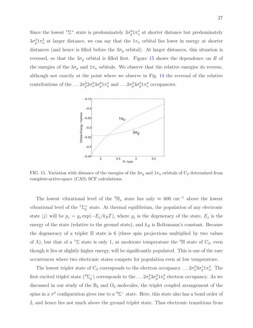
Since the lowest 1Σ+ state is predominately 3σ0g1π

4u at shorter distance but predominately

3σ2g1π

2u at larger distance, we can say that the 1πu orbital lies lower in energy at shorter

distances (and hence is filled before the 3σg orbital). At larger distances, this situation is

reversed, so that the 3σg orbital is filled first. Figure 15 shows the dependence on R of

the energies of the 3σg and 1πu orbitals. We observe that the relative energies do reverse,

although not exactly at the point where we observe in Fig. 14 the reversal of the relative

contributions of the . . . 2σ2g2σ

2u3σ

0g1π

4u and . . . 2σ2

g3σ2g1π

4u occupancies.

2 2.5 3 3.5−0.45

−0.4

−0.35

−0.3

−0.25

−0.2

−0.15

R / bohr

Orbital Energy / hartree

3σg

1πu

FIG. 15. Variation with distance of the energies of the 3σg and 1πu orbitals of C2 determined from

complete-active-space (CAS) SCF calculations.

The lowest vibrational level of the 3Πu state lies only ≈ 600 cm−1 above the lowest

vibrational level of the 1Σ+g state. At thermal equilibrium, the population of any electronic

state |j〉 will be pj = gj exp(−Ej/kBT ), where gj is the degeneracy of the state, Ej is the

energy of the state (relative to the ground state), and kB is Boltzmann’s constant. Because

the degeneracy of a triplet Π state is 6 (three spin projections multiplied by two values

of Λ), but that of a 1Σ state is only 1, at moderate temperature the 3Π state of C2, even

though it lies at slightly higher energy, will be significantly populated. This is one of the rare

occurrences where two electronic states compete for population even at low temperature.

The lowest triplet state of C2 corresponds to the electron occupancy . . . 2σ2u3σ

1g1π

3u. The

first excited triplet state (3Σ−g ) corresponds to the . . . 2σ2

u3σ2g1π

2u electron occupancy. As we

discussed in our study of the B2 and O2 molecules, the triplet coupled arrangement of the

spins in a π2 configuration gives rise to a 3Σ− state. Here, this state also has a bond order of

2, and hence lies not much above the ground triplet state. Thus electronic transitions from

28

the lowest triplet (3Πu) to the 3Σ−g state lie in the visible region of the spectrum. They are

called the “Swann” bands, and are characteristic of the spectra of burning hydrocarbons –

they are the blue color in the flame of a gas stove or in a Bunsen burner.

Problem 3 The data file C2 MRCIQ energies.txt lists, in the region of the molecular min-

imum, calculated values of V (R) for the 1Σ+g and the 3Πg states of C2. Use this data to

determine the values of Re and ωe (the vibrational frequency, in cm−1) as well as T0, the

splitting between the v = 0 vibrational levels of these two electronic states. Compare these

results with experiment Then, plot the relative Boltzmann populations of these two states

as a function of temperature over the range 200–2000 K.

C. Spectroscopic notation for diatomic molecules

Traditionally, spectroscopists label each electronic state by a letter, as well as the 2S+1Λ±g/u

lebel. The lowest state is labelled X . The excited states are then labelled alphabetically,

starting with A. Upper case letters are used for states with the same multiplicity as the

ground state, while lower case letters are used for states with a different multiplicity. Thus,

for O2, the lowest state is the X 3Σ−g state, followed, in terms of increasing energy, by the

a 1∆g and the b 1Σ+g states. For C2, the lowest state is the X 1Σ+

g , followed by the a 3Πu,

b 3Σ−g and then the A 1Πu state. Occasionally, new states are found which lie in between

previously assigned states; these states are labelled A′ or B′.

For molecular nitrogen (and molecular nitrogen only) the upper/lower case naming

scheme is reversed: The ground state is an 1Σ+g state (corresponding to the electron occu-

pancy | . . . 2σ2u3σ

2g1π

4u|) and is called the X state. However, the excited singlet states (which

have the same multiplicity as the ground state) are labelled with lower-case letters but all

the triplet states are labelled with upper-case letters.

D. States of other homonuclear diatomic molecules and ions

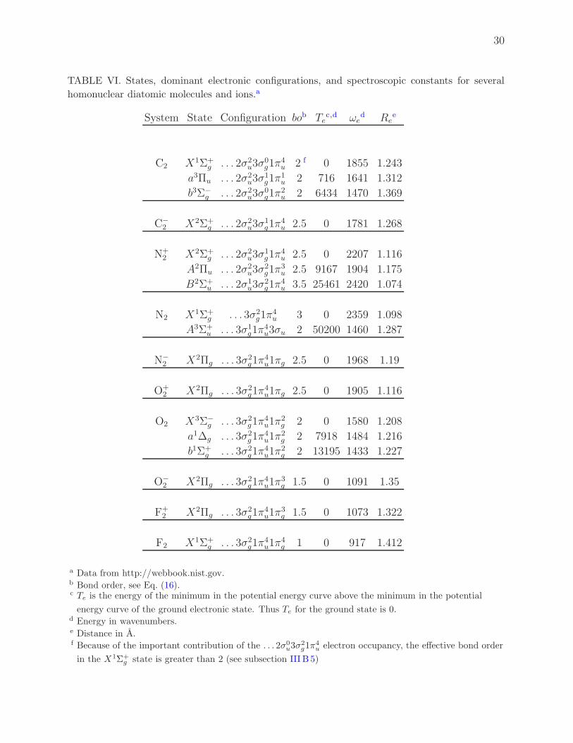
Table VI shows the dominant electronic configurations and spectroscopic constants for the

ground state and some of the lower excited states of various homonuclear diatomic molecules

and ions. We observe the correlation between bond order and the vibrational frequency and

29

internuclear distance. The higher the bond order, the stronger the bond, and the shorter

the bond length.

Problem 4 The data for N+2 in its B2Σ+

u state (see Table VI) of the N+2 ion is intriguing.

Why does this ion have the shortest bond length of any species in the table and also the

highest vibrational frequency?

Looking at the NIST Chemistry Webbook, you can find additional excited states of N+2 ,

namely the a4Σ+u , D

2Πg, and C2Σ+u states. What is a reasonable guess for the electronic

configuration of each of these states?

Note that the 2nd column contains the nominal filling of the molecular orbitals, but not

the actual Slater determinantal wavefunctions. Thus, the electronic configurations of all

the listed O2 states are identical, even though the three states correspond to the different

electronic wavefunctions discussed in the section on the O2 molecule.

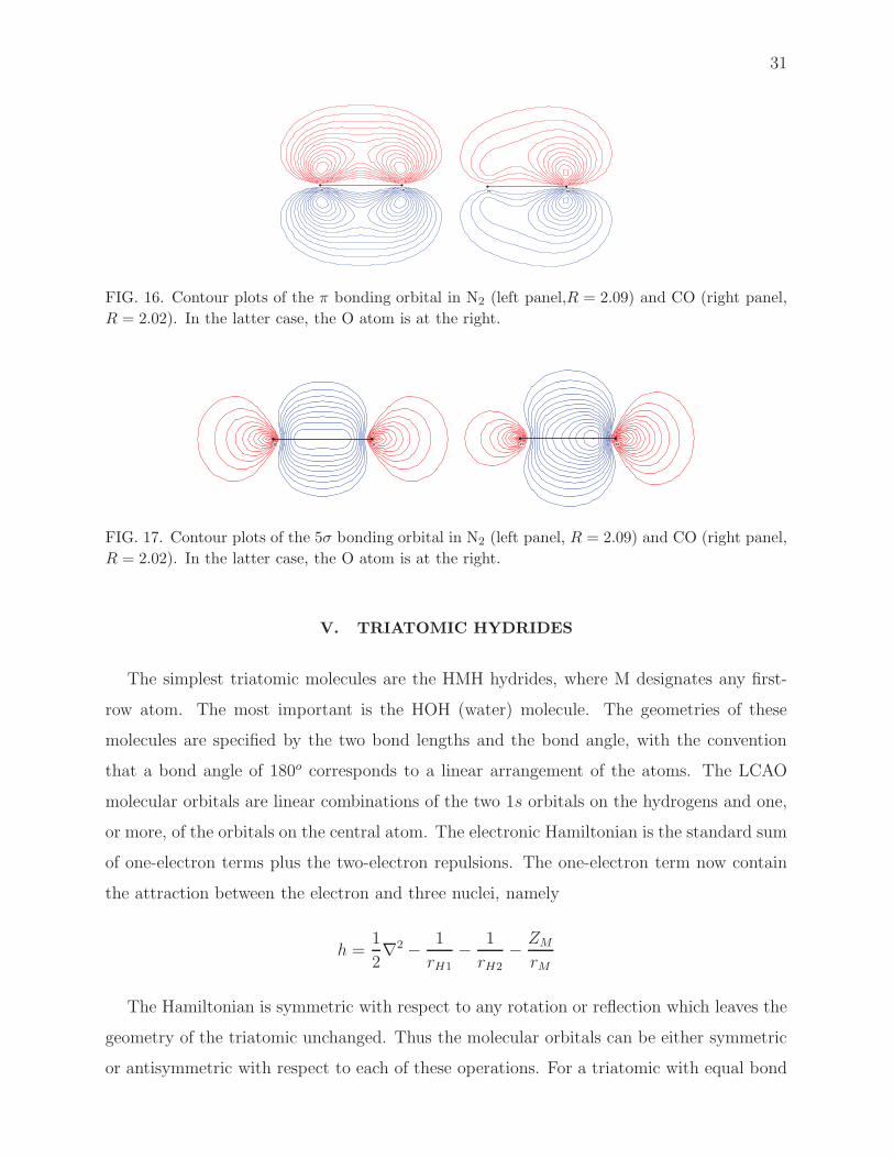
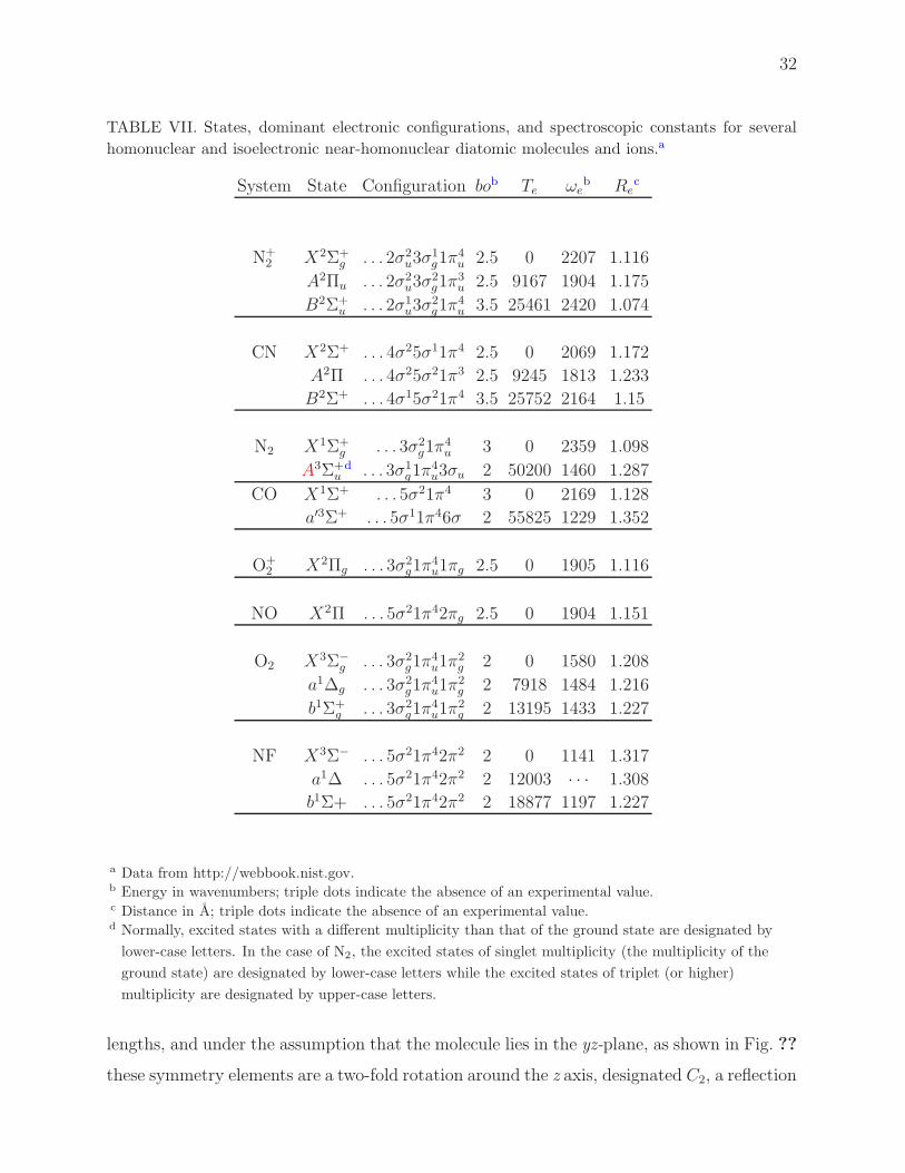
IV. NEAR-HOMONUCLEAR DIATOMICS

When the two nuclei are no longer identical, there is no longer inversion symmetry,

but the molecular orbitals still retain cylindrical symmetry. When the diatomic is nearly

homonuclear, as, for example, in the CN, CO, or NO molecules the g/u symmetry is lifted.

Usually, the lower energy molecular orbital being localized slightly more strongly on the

atom with the higher atomic number. This is illustrated in Figs. 16 and 17, which compare

for N2 and CO the bonding 5σ (3σg in the case of N2) and bonding 1π (1πu in the case of

N2) orbitals. Since the orbitals are not strongly distorted, the bonding characteristics are

little changed as is seen in Tab VII.

30

TABLE VI. States, dominant electronic configurations, and spectroscopic constants for several

homonuclear diatomic molecules and ions.a

System State Configuration bob Tec,d ωe

d Ree

C2 X1Σ+g . . . 2σ2

u3σ0g1π

4u 2 f 0 1855 1.243

a3Πu . . . 2σ2u3σ

1g1π

1u 2 716 1641 1.312

b3Σ−g . . . 2σ2

u3σ0g1π

2u 2 6434 1470 1.369

C−2 X2Σ+

g . . . 2σ2u3σ

1g1π

4u 2.5 0 1781 1.268

N+2 X2Σ+

g . . . 2σ2u3σ

1g1π

4u 2.5 0 2207 1.116

A2Πu . . . 2σ2u3σ

2g1π

3u 2.5 9167 1904 1.175

B2Σ+u . . . 2σ1

u3σ2g1π

4u 3.5 25461 2420 1.074

N2 X1Σ+g . . . 3σ2

g1π4u 3 0 2359 1.098

A3Σ+u . . . 3σ1

g1π4u3σu 2 50200 1460 1.287

N−2 X2Πg . . . 3σ2

g1π4u1πg 2.5 0 1968 1.19

O+2 X2Πg . . . 3σ2

g1π4u1πg 2.5 0 1905 1.116

O2 X3Σ−g . . . 3σ2

g1π4u1π

2g 2 0 1580 1.208

a1∆g . . . 3σ2g1π

4u1π

2g 2 7918 1484 1.216

b1Σ+g . . . 3σ2

g1π4u1π

2g 2 13195 1433 1.227

O−2 X2Πg . . . 3σ2

g1π4u1π

3g 1.5 0 1091 1.35

F+2 X2Πg . . . 3σ2

g1π4u1π

3g 1.5 0 1073 1.322

F2 X1Σ+g . . . 3σ2

g1π4u1π

4g 1 0 917 1.412

a Data from http://webbook.nist.gov.b Bond order, see Eq. (16).c Te is the energy of the minimum in the potential energy curve above the minimum in the potential

energy curve of the ground electronic state. Thus Te for the ground state is 0.d Energy in wavenumbers.e Distance in A.f Because of the important contribution of the . . . 2σ0

u3σ2g1π

4u electron occupancy, the effective bond order

in the X1Σ+g state is greater than 2 (see subsection III B 5)

31

N

N

C

O

FIG. 16. Contour plots of the π bonding orbital in N2 (left panel,R = 2.09) and CO (right panel,

R = 2.02). In the latter case, the O atom is at the right.

N

N

C

O

FIG. 17. Contour plots of the 5σ bonding orbital in N2 (left panel, R = 2.09) and CO (right panel,

R = 2.02). In the latter case, the O atom is at the right.

V. TRIATOMIC HYDRIDES

The simplest triatomic molecules are the HMH hydrides, where M designates any first-

row atom. The most important is the HOH (water) molecule. The geometries of these

molecules are specified by the two bond lengths and the bond angle, with the convention

that a bond angle of 180o corresponds to a linear arrangement of the atoms. The LCAO

molecular orbitals are linear combinations of the two 1s orbitals on the hydrogens and one,

or more, of the orbitals on the central atom. The electronic Hamiltonian is the standard sum

of one-electron terms plus the two-electron repulsions. The one-electron term now contain

the attraction between the electron and three nuclei, namely

h =1

2∇2 − 1

rH1

− 1

rH2

− ZM

rM

The Hamiltonian is symmetric with respect to any rotation or reflection which leaves the

geometry of the triatomic unchanged. Thus the molecular orbitals can be either symmetric

or antisymmetric with respect to each of these operations. For a triatomic with equal bond

32

TABLE VII. States, dominant electronic configurations, and spectroscopic constants for several

homonuclear and isoelectronic near-homonuclear diatomic molecules and ions.a

System State Configuration bob Te ωeb Re

c

N+2 X2Σ+

g . . . 2σ2u3σ

1g1π

4u 2.5 0 2207 1.116

A2Πu . . . 2σ2u3σ

2g1π

3u 2.5 9167 1904 1.175

B2Σ+u . . . 2σ1

u3σ2g1π

4u 3.5 25461 2420 1.074

CN X2Σ+ . . . 4σ25σ11π4 2.5 0 2069 1.172

A2Π . . . 4σ25σ21π3 2.5 9245 1813 1.233

B2Σ+ . . . 4σ15σ21π4 3.5 25752 2164 1.15

N2 X1Σ+g . . . 3σ2

g1π4u 3 0 2359 1.098

A3Σ+ud . . . 3σ1

g1π4u3σu 2 50200 1460 1.287

CO X1Σ+ . . . 5σ21π4 3 0 2169 1.128

a′3Σ+ . . . 5σ11π46σ 2 55825 1229 1.352

O+2 X2Πg . . . 3σ2

g1π4u1πg 2.5 0 1905 1.116

NO X2Π . . . 5σ21π42πg 2.5 0 1904 1.151

O2 X3Σ−g . . . 3σ2

g1π4u1π

2g 2 0 1580 1.208

a1∆g . . . 3σ2g1π

4u1π

2g 2 7918 1484 1.216

b1Σ+g . . . 3σ2

g1π4u1π

2g 2 13195 1433 1.227

NF X3Σ− . . . 5σ21π42π2 2 0 1141 1.317

a1∆ . . . 5σ21π42π2 2 12003 · · · 1.308

b1Σ+ . . . 5σ21π42π2 2 18877 1197 1.227

a Data from http://webbook.nist.gov.b Energy in wavenumbers; triple dots indicate the absence of an experimental value.c Distance in A; triple dots indicate the absence of an experimental value.d Normally, excited states with a different multiplicity than that of the ground state are designated by

lower-case letters. In the case of N2, the excited states of singlet multiplicity (the multiplicity of the

ground state) are designated by lower-case letters while the excited states of triplet (or higher)

multiplicity are designated by upper-case letters.

lengths, and under the assumption that the molecule lies in the yz-plane, as shown in Fig. ??

these symmetry elements are a two-fold rotation around the z axis, designated C2, a reflection

33

in the xz-plane (the plane that bisects the molecule), designated σv, and a reflection in the

yz-plane, dsignated σ′v. The group of symmetry elements of a triatomic HMH hydride is

designated C2v. The symmetries of the possible molecule orbitals with respect to these

three elements are labelled as shown in Table VIII. This table, which is called a “character

table” equilibrium distances and dissociation energies. Here E designates the unit operator.

r1 r2

z

y

θ

C2

FIG. 18. Geometry of an HMH hydride. The symmetry elements are C2, a two-fold rotation

around the z axis; σv, a reflection in the xz-plane (the plane that bisects the molecule; and σ′v, a

reflection in the yz-plane (the plane containing the molecule).

TABLE VIII. Character table for C2v symmetry.

Character E C2 σv σ′v linear, rotation quadratic

a1 +1 +1 +1 +1 z x2, y2, z2

a2 +1 +1 –1 –1 Rz xy

b1 +1 –1 +1 –1 x, Ry xz

b2 +1 –1 –1 +1 y, Rx yz

Thus any s orbital, any pz, or the dx2−y2 and dz2 atomic orbitals on the C atom belong to

the symmetry group a1, the px and the dxz orbitals belong to the symmetry group b1, and

the py and dyz orbitals belong to the symmetry group b2. Finally, the dxy orbital belongs to

the symmetry group a2.

A further introduction to molecular symmetries and group theory is contained in the

Molecular symmetry Chapter in Wikipedia.

34

We can express, generally, the molecular orbitals of H2O as linear combinations of the

two H 1s orbitals as well as the atomic orbitals on the O. Note that since the molecular

orbital must be symmetric or antisymmetric with respect to the C2 and σv operations, we

must take include both 1sH orbitals with an equal, or opposite sign. This correspond to a1

and b2 symmetry, namely

1sH(a1) = [1s1 + 1s2] (24)

and

1sH(b2) = [1s1 − 1s2] (25)

Thus, we have 7 atomic orbitals (a1 symmetry: 1s, 2s, 2pz, 1sH(a1)), b2 symmetry:

2py, 1sH(b2), and b1 symmetry 2px). Note that there are no atomic orbitals of a2 symmetry,

since there are no d orbitals in the valence basis. Within the Hartee-Fock approximation,

the ground electronic state of the H2O molecule is approximated by placing the 10 electrons

2×2 into the five lowest energy molecular orbitals. These are, to first order, the 1s and 2s

orbitals on the O atom, as well as the bonding combination of 1sH(a1) and 2pz, followed by

the bonding combination of the 1sH(b2) and 2px. The remaining two electrons go into the

2py orbital on the O, which is pointed out of the plane. This orbital is antisymmetric with

respect to reflection in the plane of the molecule (σ′v) and so will no mix with the linear

combination of the 1s(H) orbitals, both of which are symmetric with respect to σ′v.

Consequently, the electron occupancy of H2O is

ψ =∣

∣

∣1a212a213a

211b

221b

21

∣

∣

∣ ≈∣

∣

∣1s2O2s2O3a

211b

222p

2y

∣

∣

∣

Since all the orbitals are doubly filled, the overall wavefunction of the ground state of

H2O is fully symmetric, with spin zero. The lowest electronic state of H2O is designated 1A1.

Here, the tilde indicates that we are referring to a triatomic molecule. With this electron

occupancy, one determines the best one-electron functions, by allowing each electron to move

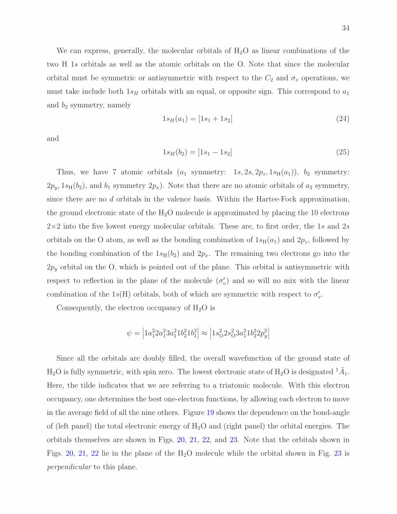
in the average field of all the nine others. Figure 19 shows the dependence on the bond-angle

of (left panel) the total electronic energy of H2O and (right panel) the orbital energies. The

orbitals themselves are shown in Figs. 20, 21, 22, and 23. Note that the orbitals shown in

Figs. 20, 21, 22 lie in the plane of the H2O molecule while the orbital shown in Fig. 23 is

perpendicular to this plane.

35

80 100 120 140 160 1800

0.01

0.02

0.03

0.04

0.05

0.06

θ / degree

E−

Em

in / h

art

ree

θmin

=104.4

60 80 100 120 140 160 180−1.4

−1.2

−1

−0.8

−0.6

−0.4

θ /degree

orb

ita

l e

ne

rgy / h

art

ree

2a1

3a1

1b2

1b1

FIG. 19. (left panel) Energy of the H2O molecule in the 1A1 state as a function of the bond angle,

from Hartree-Fock calculations with a double-zeta basis set. The energy at the minimum is –76.03

hartree. (right panel) Energies (in hartree) of the orbitals of the H2O molecule (with the exception

of the 1sO orbital) as a function of the bond angle.

220

O

H H

221

O H H

2σ 2a1

θ=180 θ=104

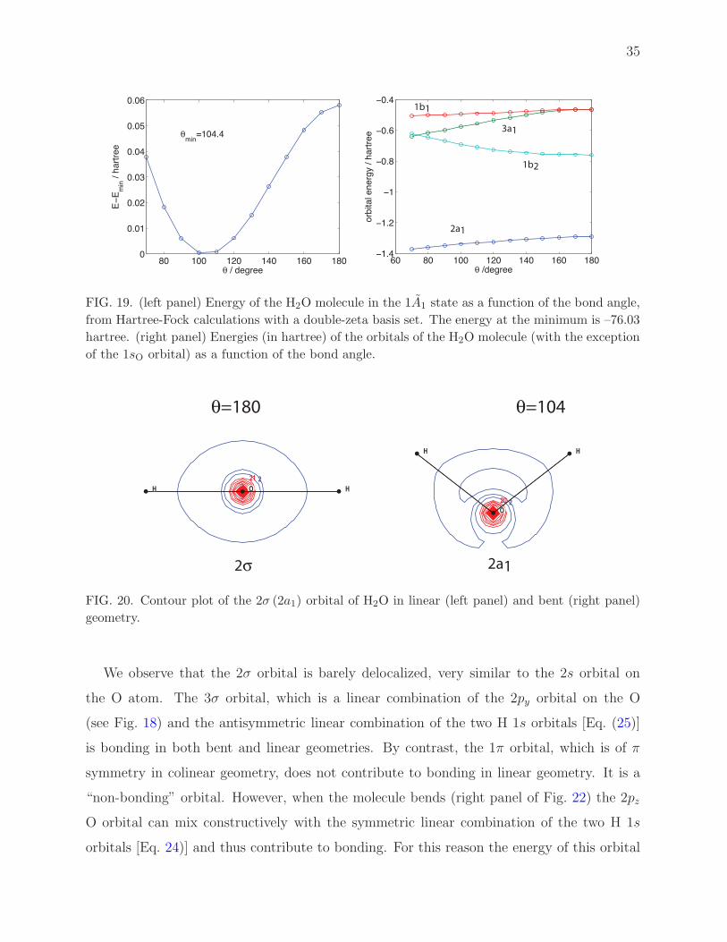
FIG. 20. Contour plot of the 2σ (2a1) orbital of H2O in linear (left panel) and bent (right panel)

geometry.

We observe that the 2σ orbital is barely delocalized, very similar to the 2s orbital on

the O atom. The 3σ orbital, which is a linear combination of the 2py orbital on the O

(see Fig. 18) and the antisymmetric linear combination of the two H 1s orbitals [Eq. (25)]

is bonding in both bent and linear geometries. By contrast, the 1π orbital, which is of π

symmetry in colinear geometry, does not contribute to bonding in linear geometry. It is a

“non-bonding” orbital. However, when the molecule bends (right panel of Fig. 22) the 2pz

O orbital can mix constructively with the symmetric linear combination of the two H 1s

orbitals [Eq. 24)] and thus contribute to bonding. For this reason the energy of this orbital

36

decreases dramatically as the molecule bends (this can be seen in the right panel of Fig. 19.

There is one more doubly-filled orbital in H2O. This orbital corresponds to the out of

plane 2px orbital on the O atom. It has symmetry πx in linear geometry and b1 in bent

geometry. This orbital never contributes to bonding. The two electrons in this orbital are

called, hence, a “lone-pair”. The geometry of the H2O molecule can not be predicted on

2

O H H

3σ = 1b2

2

O

H H

θ=180 θ=104

FIG. 21. Contour plot of the 3σ (1b2) orbital of H2O in linear (left panel) and bent (right panel)

geometry.

O

H H

O H H

1π

θ=180 θ=104

3a1

FIG. 22. Contour plot of the 3σ (3a1) orbital of H2O in linear (left panel) and bent (right panel)

geometry.

the basis of simple Lewis dot structures. Further, in the usual partial-charge model of water

(see Fig. 24) the positive charges on the protons should repel one-another which would lead

37

15

O

H H

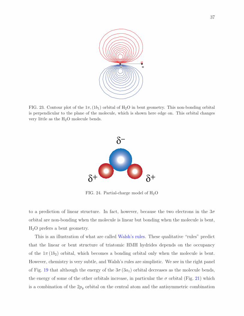
FIG. 23. Contour plot of the 1π, (1b1) orbital of H2O in bent geometry. This non-bonding orbital

is perpendicular to the plane of the molecule, which is shown here edge on. This orbital changes

very little as the H2O molecule bends.

δ–

δ+ δ+

FIG. 24. Partial-charge model of H2O

to a prediction of linear structure. In fact, however, because the two electrons in the 3σ

orbital are non-bonding when the molecule is linear but bonding when the molecule is bent,

H2O prefers a bent geometry.

This is an illustration of what are called Walsh’s rules. These qualitative “rules” predict

that the linear or bent structure of triatomic HMH hydrides depends on the occupancy

of the 1π (1b2) orbital, which becomes a bonding orbital only when the molecule is bent.

However, chemistry is very subtle, and Walsh’s rules are simplistic. We see in the right panel

of Fig. 19 that although the energy of the 3σ (3a1) orbital decreases as the molecule bends,

the energy of some of the other orbitals increase, in particular the σ orbital (Fig. 21) which

is a combination of the 2py orbital on the central atom and the antisymmetric combination

38

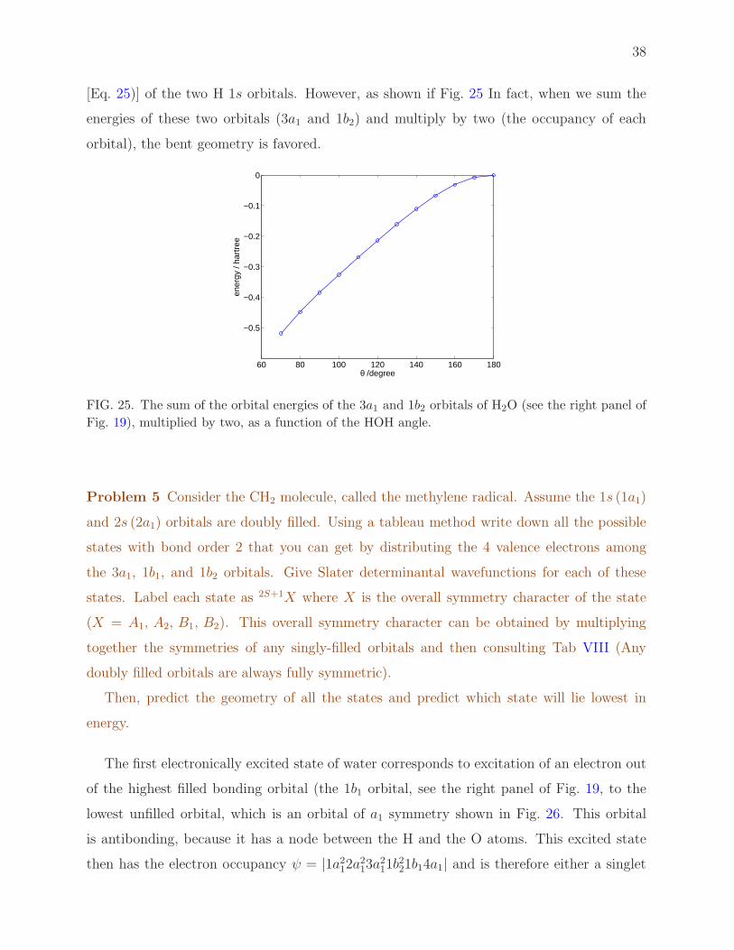
[Eq. 25)] of the two H 1s orbitals. However, as shown if Fig. 25 In fact, when we sum the

energies of these two orbitals (3a1 and 1b2) and multiply by two (the occupancy of each

orbital), the bent geometry is favored.

60 80 100 120 140 160 180

−0.5

−0.4

−0.3

−0.2

−0.1

0

θ /degree

ener

gy /

hart

ree

FIG. 25. The sum of the orbital energies of the 3a1 and 1b2 orbitals of H2O (see the right panel of

Fig. 19), multiplied by two, as a function of the HOH angle.

Problem 5 Consider the CH2 molecule, called the methylene radical. Assume the 1s (1a1)

and 2s (2a1) orbitals are doubly filled. Using a tableau method write down all the possible

states with bond order 2 that you can get by distributing the 4 valence electrons among

the 3a1, 1b1, and 1b2 orbitals. Give Slater determinantal wavefunctions for each of these

states. Label each state as 2S+1X where X is the overall symmetry character of the state

(X = A1, A2, B1, B2). This overall symmetry character can be obtained by multiplying

together the symmetries of any singly-filled orbitals and then consulting Tab VIII (Any

doubly filled orbitals are always fully symmetric).

Then, predict the geometry of all the states and predict which state will lie lowest in

energy.

The first electronically excited state of water corresponds to excitation of an electron out

of the highest filled bonding orbital (the 1b1 orbital, see the right panel of Fig. 19, to the

lowest unfilled orbital, which is an orbital of a1 symmetry shown in Fig. 26. This orbital

is antibonding, because it has a node between the H and the O atoms. This excited state

then has the electron occupancy ψ = |1a212a213a211b221b14a1| and is therefore either a singlet

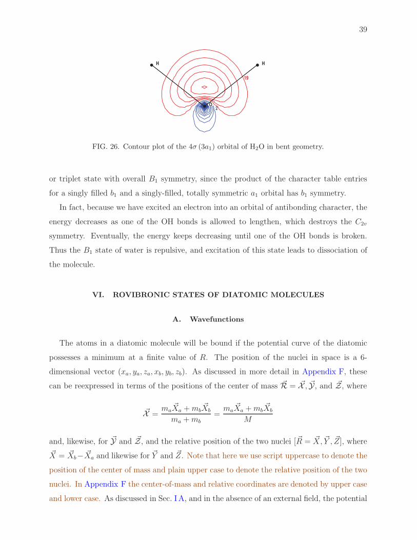
39

2

19

O

H H

FIG. 26. Contour plot of the 4σ (3a1) orbital of H2O in bent geometry.

or triplet state with overall B1 symmetry, since the product of the character table entries

for a singly filled b1 and a singly-filled, totally symmetric a1 orbital has b1 symmetry.

In fact, because we have excited an electron into an orbital of antibonding character, the

energy decreases as one of the OH bonds is allowed to lengthen, which destroys the C2v

symmetry. Eventually, the energy keeps decreasing until one of the OH bonds is broken.

Thus the B1 state of water is repulsive, and excitation of this state leads to dissociation of

the molecule.

VI. ROVIBRONIC STATES OF DIATOMIC MOLECULES

A. Wavefunctions

The atoms in a diatomic molecule will be bound if the potential curve of the diatomic

possesses a minimum at a finite value of R. The position of the nuclei in space is a 6-

dimensional vector (xa, ya, za, xb, yb, zb). As discussed in more detail in Appendix F, these

can be reexpressed in terms of the positions of the center of mass ~R = ~X , ~Y, and ~Z, where

~X =ma

~Xa +mb~Xb

ma +mb=ma

~Xa +mb~Xb

M

and, likewise, for ~Y and ~Z, and the relative position of the two nuclei [~R = ~X, ~Y , ~Z], where

~X = ~Xb− ~Xa and likewise for ~Y and ~Z. Note that here we use script uppercase to denote the

position of the center of mass and plain upper case to denote the relative position of the two

nuclei. In Appendix F the center-of-mass and relative coordinates are denoted by upper case

and lower case. As discussed in Sec. IA, and in the absence of an external field, the potential

40

depends only on the magnitude of ~R. The Hamiltonian is separable so that the wavefunction

for the motion of the two nuclei can be written as a product of the wavefunction for the

position of the center-or-mass Ψ(X ,Y ,Z) multiplied by the wavefunction for the relative

motion of the two nuclei ψ(X, Y, Z). The energy is the sum of the energy associated with

the motion of the center of mass and the energy associated with the relative motion, namely

− 1

2M∇2

RΨ(X ,Y ,Z) = ECMΨ(X ,Y ,Z) (26)

and[

− 1

2µ∇2

R + V(k)eff (R)

]

ψ(X, Y, Z) = Eintψ(X, Y, Z) (27)

Here V(k)eff (R) is the effective (Born-Oppenheimer) potential in the kth electronic state for

the motion of the nuclei: the sum of the electronic energy plus the repulsion between the

two nuclei.

The motion of the center of mass is that of a particle in a cubic box (no potential), so

that the motion of the molecule in space has the same wavefunctions and energies as that

of a particle in a box with mass equal to the total mass of the molecule. We shall label the

wavefunction by the three particle-in-a-box quantum numbers, namely ΨNX ,NY ,NZ.

In Eq. (27), the potential depends only on the distance between the two nuclei. Thus, as in

the case of the hydrogen atom, the Hamiltonian is separable in spherical polar coordinates.

The wavefunction may be written as the product of a spherical harmonic in the angular

degrees of freedom (the orientation of ~R) multiplied by a function which depends only on R

(you may be more familiar with this as the radial function R(R) in the case of the hydrogen

atom) which satisfies the equation

[

− 1

2µR2

d

dR

(

R2 d

dR

)

+j(j + 1)

2µR2+ V

(k)eff(R)

]

χvj(R) = Eintχvj(R) (28)

The complete wavefunction is then

Ξ(X ,Y ,Z, R,Θ,Φ, ~r) = ΨNX ,NY ,NZ(X ,Y ,Z)ψk,v,j,m(X, Y, Z)

where

ψk,v,j,m(X, Y, Z) = Yjm(Θ,Φ)χvj(R)χ(k)el (~r;R) (29)

41

where ~r denotes collectively the coordinates of all the electrons. Here k is the electronic

state index (or quantum number), v is the vibrational quantum number, j is the rotational

quantum number, andm is the projection of the rotational angular momentum (−m ≤ j m).

If the potential curve V(k(eff(R) has a minimum, then the internal energy (the molecular

energy independent of the motion of its center of mass through space) will correspond to

a particular electronic-vibration-rotation (or “rovibronic”) state, which we label with the

quantum numbers {k, v, j,m}, where m is the projection of ~j.

B. Energies

To determine these internal energies of the diatomic molecule, we need to solve Eq. (27).

An analytic solution is not possible for most realistic molecular potentials. To approximate

the energies, we expand the potential about R = Re, the minimum in V(k)eff , namely

V (R) ≈ V (Re) +1

2

d2V

dR2

∣

∣

∣

∣

∣

Re

x2 +1

6

d3V

dR3

∣

∣

∣

∣

∣

Re

x3 +1

24

d4V

dR4

∣

∣

∣

∣

∣

Re

x4 + . . .

where x ≡ R − Re and where, for simplicity, we have suppressed the subscript “eff” and

superscript (k). Note that the first derivative of the potential vanishes at R = Re. We can

also expand the rotational angular momentum term depending on 1/R2 by noting that

1

R2=

1

(Re + x)2=

1

R2e(1 + x/Re)2

≈ 1

R2e

(

1− x

Re+ 2

x2

R2e

− 3x3

R3e

+ 4x4

R4e

+ . . .

)

We can now use time-independent perturbation theory, so that

Eint ≈ E(0) +⟨

φ(0)v

∣

∣

∣H ′∣

∣

∣φ(0)v

⟩

We separate the Hamiltonian as

Ho =j(j + 1)

2µR2e

+ V (Re) +1

2

d2V

dR2

∣

∣

∣

∣

∣

Re

x2

and

H ′ =j(j + 1)

2µR2e

(

− x

Re

+x2

R2e

− x2

R3e

+x4

R4e

)

+1

6

d3V

dR3

∣

∣

∣

∣

∣

Re

x3 +1

24

d4V

dR4

∣

∣

∣

∣

∣

Re

x4 (30)

42

Thus, the zero-order wavefunctions and energy levels are those of a Harmonic oscillator

with force constant

k =d2V

dR2

∣

∣

∣

∣

∣

Re

and energies [note that the term j(j + 1)/(2µR2e) leads to a j-dependent addition to the

energy]

E(0)v,j = V (Re) +Bj(j + 1) +

(

v +1

2

)

hω (31)

where the rotational constant Be is defined by (here, for generality, we have included explic-

itly the factor of h)

B =h2

2µR2e

and the vibrational frequency is defined by ω =√

k/µ. Typically, the potential is defined

so that

limR→∞

V (R) = 0

so that V (Re) = −De, where De is the dissociation energy of the molecule, which is defined

as a positive number. Thus, we can rewrite Eq. (31) as

E(0)v,j = −De +Bj(j + 1) +

(

v +1

2

)

hω (32)

The first-order correction to the energy is

E(1)v,j = 〈v|H ′ |v〉 = 〈v| j(j + 1)

2µR2e

[

− x

Re

+ 2x2

R2e

+ 3x3

R3e

− 4x4

R4e

]

|v〉

+ 〈v| 16

d3V

dR3

∣

∣

∣

∣

∣

Re

x3 +1

24

d4V

dR4

∣

∣

∣

∣

∣

Re

x4 + . . . |v〉 (33)

By symmetry 〈v|x|v〉 = 〈v|x3|v〉 = 0. From the Matlab script quartic oscillator variational.m,

you can show that

〈v|x2|v〉 = (v + 1/2)h√kµ

= (v + 1/2)h

µω(34)

and

〈v|x4|v〉 =[

12(v + 1/2)2 + 3] h2

8kµ=[

12(v + 1/2)2 + 3] h2

8(µω)2. (35)

43

Thus,

E(1)v,j = h

(v + 1/2)j(j + 1)

R4eµ

3/2k1/2+ h2

[

1

24

d4V

dR4

∣

∣

∣

∣

∣

Re

+j(j + 1)

2µR6e

] [

12(v + 1/2)2 + 3

8kµ

]

(36)

Problem 6 Use the Matlab script quartic oscillator variational.m to generate expressions

for 〈v|x4|v〉 for v = 0 − 5. Show that they correspond to the analytic formula given in

Eq. (35).

To evaluate the second-order contributions to the energy, we need the off-diagonal matrix

elements of xn (n = 1 − 4) in the harmonic oscillator basis. In general a term in xn in H ′

[Eq. 30)] will make a second-order contribution of

E(2)vj =

∑

v′ 6=v

|〈v|xn|v′〉|2Ev −Ev′

=∑

v′ 6=v

|〈v|xn|v′〉|2(v − v′)ω

The Hermite polynomials satisfy a two-term recursion relation

xHm(x) =1

2Hm+1(x) +mHm−1(x)

Thus, acting on Hm(x) by xn will generate polynomials up to order Hm+n(x). Consequently,

the orthogonality and symmetry properties of the Hermite polynomials will guarantee that

〈v|xn |v′〉 = 0 for v′ > v + n

Furthermore, by symmetry, if n is odd then

〈v|xn |v′〉 = 0

if v and v′ are both odd or both even. Similarly, if n is even, then the matrix element will

vanish if v is odd and v′ is even, or vice versa. The script quartic oscillator variational.m

generates the matrices 〈v|xn|v′〉 for 0 ≤ v ≤ 6 and n = 1−4. From the output of this script,

specifically the matrix x1mat, you can show that, for v′ > v

〈v|x|v′〉 =[

2(v + 1/2) + 1

4kµ

]1/2

, for v′ = v + 1

= 0, otherwise (37)

44

(with a similar relation when v′ < v). Likewise, from the matrix x2mat you can show that,

for v′ > v

〈v|x2|v′〉 =[

4(v + 1/2)2 + 8(v + 1/2) + 3

16kµ

]1/2

, for v′ = v + 2

= 0, otherwise (38)

Similarly, from the matrix x3mat you can show that, for v′ > v

〈v|x3|v′〉 =[

72(v + 1/2)3 + 108(v + 1/2)2 + 54(v + 1/2) + 9

64kµ

]1/2

, for v′ = v + 1

=

[

8(v + 1/2)3 + 36(v + 1/2)2 + 46(v + 1/2) + 15

64kµ

]1/2

, for v′ = v + 3

= 0, otherwise (39)

Examining the equations for the zeroth and first-order energies, we see that the total

internal energy of a diatomic can be expressed, most generally then as a dual power series

in (v + 1/2) and j(j + 1), namely

Ev,j = −De + Y00 + Y10(v + 1/2) + Y01j(j + 1) + Y11(v + 1/2)j(j + 1)

+Y20(v + 1/2)2 + Y21j(j + 1)(v + 1/2)2 + . . . (40)

The Ymn coefficients are called Dunham Coefficients. In principle, by means of perturbation

theory one can relate the values of these coefficients to the physical parameters which define

the molecular potential V (R) as well as the reduced mass of the molecule. Alternatively,

spectroscopists often fit the results of experiments to the following (virtually identical )

double power series

Ev,j = (v + 1/2)ωe − (v + 1/2)2ωexe + (v + 1/2)3ωeye

+j(j + 1)Be − j(j + 1)(v + 1/2)αe (41)

Note that the coefficient αe is unrelated to the parameter α which appears in the expression

for the harmonic oscillator wavefunctions. We can combine the last two terms in Eq. (41 to

obtain

Ev,j = . . .+ j(j + 1)Be − j(j + 1)(v + 1/2)αe = . . .+ j(j + 1)Bv

45

where Bv, the effective rotational constant in vibrational level v is

Bv = Be − αe(v + 1/2)

The expansion coefficients in Eq. (41), often called “spectroscopic coefficients”, as well as

the Dunham coefficients, are typically given in cm−1 units, so that the resulting “energy” is

proportional to the level energy but needs to be multiplied by hc to obtain the a result in

units of energy.

C. Physical interpretation of the spectroscopic expansion coefficients

The Dunham coefficients can be related by perturbation theory to the reduced mass of

the molecule and to the derivatives of the potential curve, while the expansion coefficients

of Eq. (41) are empirical parameters. However, the two expansions are closely related. In

particular:

i. Y10 (or ωe) is the vibrational frequency of the molecule, related to the curvature (the

second derivative) of the potential Veff(R) at its minimum. Since, for a classical oscillator,

ω =√

k/µ, for chemically indentical, but isotopically distinct, species (such as HF/DF

or 12CO/13CO) the vibrational frequency is proportional to the inverse square root of the

reduced mass. For diatomic hydrides ωe is typically between 3000 and 4000 cm−1. For

non-hydride diatomics ωe is typically between 1000 and 2500 cm−1.

ii. Y20 (or ωexe) is the effect of the anharmonicity of Veff(R), resulting in a decrease in

the vibrational energy spacing as the vibrational quantum number increases. Note that

the ωexe term in Eq. (41) occurs with a negative sign, whereas in the Dunham expansion

[Eq. (40)] the Y20 term enters with a positive sign. In nearly all cases ωexe is positive and,

correspondingly, Y20 is negative. Typically, ωexe is 1/20 – 1/10 of the value of the vibrational

frequency.

iii. Y30 (or ωeye) is a higher-order harmonic correction. The value of ωeye is always very

small.

iv. Y01 (or Be) is the rotational constant, related, inversely, to the square of the bond length

at equilibrium. For chemically indentical, but isotopically distinct, species the vibration

frequency is proportional to the inverse of the reduced mass. Typically, for hydrides, Be

46

is on the order of tens of wavenumbers. For non-hydride diatomics, Be is typically on the

order of 1–2 cm−1.

Extraction of Be from an experiment is the best way to determine the bond length of a

molecule. For polyatomic molecules, most rotational transitions lie in the microwave region

of the spectrum. Advances in microwave technology, stimulated by the large investment

in radar during the 2nd World War, allowed the determination of the geometry (bond

lengths and bond angles) of many small polyatomic molecules. By isotopic substitution of

the parent molecule, which generated a different pattern of rotational levels, and, hence,

different rotational constants, one could determine geometries of even complex molecules

without ambiguity.

v. Y11 (or αe) is the change in the rotational constant upon vibrational excitation. A

rotating, vibrating molecule has an effective rotational constant Bv = 〈v|1/(2µR2)|v〉. As

the vibrational quantum number increases, because of the anharmonicity of the molecular

potential the wavefunction will extend to larger and larger values of R. Thus, the effective

value of 1/R2 (and, hence, the rotational constant) will become smaller. Note that the αe

term in Eq. (41) occurs with a negative sign, whereas in the Dunham expansion [Eq. (40)] the

Y11 term enters with a positive sign. In nearly all cases αe is positive and, correspondingly,

Y11 is neagtive. For most molecules, the magnitude of αe is 1–2% the value of the rotational

constant.

vi. A smaller term which we have not included in Eqs. (40) and (41) is called the centrifugal

distortion constant [Y02 or De (no relation to the dissociation energy)]. As the molecule

rotates faster and faster, the increasing size of the j(j + 1)/2µR2 term in Eq. (28) will shift

the minimum in the potential to larger values of R. This will result in a slight decrease

in the effective rotational constant. The constants Y02 and De are, consequently, negative.

Typically the magnitude of De is no larger than 1% of the magnitude of Be.

vi. The constant term Y00 does not appear in the most common spectroscopic expansion

[Eq. (41)]. Since the Y00 term affects equally the energy of any vibration-rotation level, it

is difficult to deduce from a spectroscopic experiment which measures differences between

energy levels. Both Y00 and the dissociation energy De provide the constant term in the

expansion of Eq. (40). However, the magnitude of Y00 is a very small fraction of molecular

dissociation energies which are typically 50,000 – 100,000 cm−1. Usually, molecular disso-

ciation energies are deduced by thermochemical measurements (heats of reaction, heats of

47

formation). Consequently, one would need extremely high precision in these thermochemical

measurements to allow an accurate determination of Y00.

Problem 7 For the H2 molecule, Re = 0.74144 A, ωe = 4401.2 cm−1, and De = 38297 cm−1.

Determine the parameter β (in bohr−1) in a Morse fit to the potential curve for H2

V (R) = De {exp [−2β(R− Re)]− 2 exp [−β(R− Re)]}