Embed Size (px)
Citation preview

UNLV Theses, Dissertations, Professional Papers, and Capstones
12-15-2019
Moisture Dynamics of a Near-Surface Desert Soil Moisture Dynamics of a Near-Surface Desert Soil
Yuan Luo
Follow this and additional works at: https://digitalscholarship.unlv.edu/thesesdissertations
Part of the Geology Commons
Repository Citation Repository Citation Luo, Yuan, "Moisture Dynamics of a Near-Surface Desert Soil" (2019). UNLV Theses, Dissertations, Professional Papers, and Capstones. 3822. http://dx.doi.org/10.34917/18608713
This Dissertation is protected by copyright and/or related rights. It has been brought to you by Digital Scholarship@UNLV with permission from the rights-holder(s). You are free to use this Dissertation in any way that is permitted by the copyright and related rights legislation that applies to your use. For other uses you need to obtain permission from the rights-holder(s) directly, unless additional rights are indicated by a Creative Commons license in the record and/or on the work itself. This Dissertation has been accepted for inclusion in UNLV Theses, Dissertations, Professional Papers, and Capstones by an authorized administrator of Digital Scholarship@UNLV. For more information, please contact [email protected].

MOISTURE DYNAMICS OF A NEAR-SURFACE DESERT SOIL
By
Yuan Luo
Bachelor of Science – Engineering of Water Resources and Electric PowerNorth China University of Water Resources and Electric Power, Zhengzhou, China
2011
Master of Science – Civil EngineeringUniversity of Kansas, Lawrence
2013
A dissertation submitted in partial fulfillmentof the requirements for the
Doctor of Philosophy – Geoscience
Department of GeoscienceCollege of Sciences
The Graduate College
University of Nevada, Las VegasDecember 2019

Copyright by Yuan Luo, 2020
All Rights Reserved

ii
Dissertation Approval
The Graduate College The University of Nevada, Las Vegas
November 14, 2019
This dissertation prepared by
Yuan Luo
entitled
Moisture Dynamics of a Near-Surface Desert Soil
is approved in partial fulfillment of the requirements for the degree of
Doctor of Philosophy – Geoscience Department of Geoscience
Markus Berli, Ph.D. Kathryn Hausbeck Korgan, Ph.D. Examination Committee Chair Graduate College Dean Ganqing Jiang, Ph.D. Examination Committee Member David Kreamer, Ph.D. Examination Committee Member Elisabeth Hausrath, Ph.D. Examination Committee Member Dale Devitt, Ph.D. Graduate College Faculty Representative

iii
ABSTRACT
MOISTURE DYNAMICS OF A NEAR-SURFACE DESERT SOIL
By
Yuan Luo
Dr. Markus Berli, Examination Committee Chair
Associate Research Professor of Environmental Physics
Division of Hydrologic Sciences
Desert Research Institute, Las Vegas
Desert soils cover about one third of the Earth’s land surface. Despite their large extent
and critical role for infiltration, redistribution and evapotranspiration of the sparse precipitation
in desert environments, our understanding of desert soil hydraulic processes and properties is still
rather limited. In particularly with respect to the near-surface (top centimeters) of the soil profile,
which hosts most of the biologic activity and controls runoff, erosion as well as the emission of
dust (Nannipieri et al.,2003; Bradford et al.,1987). Deserts are also ideal locations for electricity
generation with solar energy using large-scale photovoltaic (PV) facilities with considerable
impacts on desert environments. To minimizing these impact (Sinha et al. 2018) a better
understanding is needed how facility-scale solar PV installations may affect the local hydrology,
in particular the moisture distribution in the soil underneath and between rows of solar panels.
A recent study by Dijkema et al. (2018) introduced a modeling framework to simulate the
moisture dynamics of bare, desert soil. Their model was able to capture water redistribution
under infiltration as well as evaporation conditions. For the latter, however, only when the soil
iv
was relatively moist (volumetric moisture content >10%, matric head <pF 2). For dryer soil
conditions, however, as they occur between rainfall events and are typical for desert soils most of
the time, the model consistently underestimated evaporative fluxes and, subsequently,
overestimated soil moisture content. The goal of this study was therefore to improve the model
by Dijkema et al. (2018) by using the Peters-Durner-Iden (or PDI) water retention and hydraulic
conductivity functions (Peters, 2013, 2014) to capture not only capillary but also film flow of
liquid water in the soil pores to better simulate the moisture dynamics of bare, near-surface
desert soils.
I found that the PDI water retention functions better represent measured water retention
curves than the bimodal van Genuchten (or BVG) water retention functions used by Dijkema et
al. (2018). In particular for the critical range of volumetric moisture contents between 5% and
10% (corresponding saturation degrees between 16% and 32%, and matric heads between pF 2
and pF 4). The BVG water retention functions predicted higher suctions (lower matric heads)
than the PDI functions for volumetric moisture contents in the range from 5% to 10%, likely
leading to an underestimation of the hydraulic conductivity values and water fluxes in the soil in
the range from 5% to 10%. Interestingly, the BVG and PDI hydraulic conductivity functions
were not noticeably different within the range between pF 2 and 3. For pF values higher than 3,
however, the PDI functions predicted higher hydraulic conductivity values than the BVG
functions. Therefore, the hypothesis put forward by Dijkema et al. (2018) that including film
flow may improve model predictions could be confirmed for pF >3. For pF values between 2 and
3, however, is probably rather the difference between BVG and PDI water retention functions
than hydraulic conductivity functions that led to the improved soil moisture simulations. Using
PDI instead of BVG hydraulic functions, the improved model by Dijkema et al. (2018) (hereafter
v
referred to as Luo et al., 2019a) was able to much better simulate measured soil moisture data
from the SEPHAS Lysimeter 1 (https://www.dri.edu/sephas) at 10 cm depth and below.
To further test the model by Luo et al. (2019a), I compared simulated with measured
moisture data from the top 50 mm of SEPHAS Lysimeter 1 soil that were instrumented with an
array of Triple-Point-Heat-dissipation Probes (TPHP, East 30 Sensors, Inc., Pullman, WA).
These TPHPs allow to monitor volumetric soil moisture content and temperature near the soil
surface from 0 mm to 54 mm depth at 6 mm vertical intervals on an hourly basis. The TPHPs
provided a unique dataset that captured the moisture distribution of the near surface soil for
nearly a decade. The measured soil moisture dataset showed that only the top 20 mm of the soil
dry out completely (i.e. reach a moisture content below the detection limit of the TPHP) when no
precipitation occurs for several months such as during summer and fall 2019. The soil moisture
contents between 20 to 50 mm depths, however, convert towards some equilibrium value ranging
between 3.5% and 5% (or 15% to 21% saturation, respectively). I compared measured soil
moisture time series for different depth with simulations using the model by Luo et al. (2019a)
and found that the latter is able to quite accurately forward simulate soil moisture redistribution
in the top 50 mm of the soil profile for a wide range of soil moisture contents ranging from 15%
to over 90% saturation using only independently determined soil physical parameters as well as
precipitation and evaporation as flux boundary conditions. Measurements and simulations show
that soil moisture from the top 50 mm evaporates back into the atmosphere within one month or
less after a rain event. The spatial and temporal soil moisture distribution of the top 50 mm
during evaporation point toward a two-step evaporation process as proposed by Shokri et al.
(2009) and Or et al. (2013), which could not be fully captured by Luo et al. (2019b).

vi
In a third step, I applied the model by Luo et al. (2019a) to explore the impact of solar
arrays on the moisture distribution in the soil of a PV solar facility with its characteristic rows of
solar panels that change the way rainwater reaches the soil and, therefore, likely also the local
hydrology at a PV solar facility. I was particularly interested in how solar arrays may lead to
concentrated infiltration of rainwater into the soil and whether this change of infiltration pattern
has an impact on the water balance of the soil within the solar facility. For this purpose, I set up a
process-based soil physics model with HYDRUS-2D for the soil of the “Solar 1” PV solar
facility at the Desert Research Institute (DRI) in Las Vegas (http://www.dri.edu/renewable-
energy#Solar-Generation). Solar 1 consists of 204 PV solar panels, has a nominal output of 54
kW, and produces electricity for DRI’s Las Vegas campus. Soil physical processes were
simulated based on Luo et al. (2019a) and soil physical properties were determined from soil
samples collected at Solar 1. Model-calculations were driven by measured precipitation and
calculated evaporation data taking measured air-temperature, net radiation, relative humidity and
wind speed into account using data from nearby CEMP station at DRI Las Vegas
(https://cemp.dri.edu/cgibin/cemp_stations.pl?stn=lasv). Measured and simulated water content
values from three depth in the drip line, between panels and underneath panels were compared to
evaluate the model.
The HYDRUS-2D simulations showed that the solar PV panels concentrate rainfall along
the drip lines of the panels, which causes deeper infiltration of rainwater along the drip lines
compared to areas between rows and no infiltration underneath a row of solar PV panels. This
finding is in accordance with recent lysimeter studies on infiltration into and evaporation off
bare, arid soil (Koonce, 2016; Lehmann et al., 2019) that shown that the deeper rainwater
infiltrates into the soil, the less likely it is to evaporate back into the atmosphere. HYDRUS-2D

vii
calculated agreed best with measured moisture content values from the soil at the drip line and
underneath the panels. The former is quite interesting since the drip line is the area with the
highest moisture dynamics. The latter is less surprising since not much soil moisture change
occurs underneath the panel. The HYDRUS-2D model, however, had only limited success in
simulating the moisture content of the soil between the panels. A possible reason is that the soil
between the panels is more heterogenous than assumed by the HYDRUS-2D model. It was also
noticed that during rain events water tend to pond on the soil between panels, which HYDRUS-
2D cannot take into account but may also considerably affect infiltration and water redistribution
of rainwater within the soil between panel.
In conclusions, the model by Luo et al. (2019a) can accurately simulate moisture content
values as low as 3.5% (corresponding to 15% saturation and pF 4.7) when using the PDI instead
of the BVG water retention and hydraulic conductivity functions. Provided good quality water
retention and hydraulic conductivity data are available to parametrize the PDI functions. I.e. the
model by Luo et al. (2019a) is able to simulate the moisture dynamics of a bare, near-surface
desert soil from near-saturation to about twice the air-dry moisture content. The study also shows
how the soil moisture distribution in the top 50 mm of a bare desert soil changes as a function of
individual precipitation events as well as evaporation for several months without precipitation.
HYDRUS-2D simulations in combination with measurements showed how rows of PV solar
panels affect the soil moisture distribution between and underneath the panels and how initial, or
antecedent, moisture content plays a role in terms of infiltration pattern.
Further research is needed to explore whether the PDI model could capture water
redistribution at volumetric soil moisture contents even lower than 3.5% (pF >4.7), maybe as low
as 2%, which would correspond to air-dry conditions for Lysimeter 1 soil assuming an average
viii
air relative humidity of 60% (at 25˚C). The PDI model (Peters, 2013) includes a vapor flow
component, which has not been taken into account for this study but could be employed to
simulate water flow in the vapor phase necessary to simulate the water dynamics at even lower
moisture content. In terms of water redistribution due to PV solar panels, a follow up study that
simulates a series of storms events over say a one year period could shed light on whether areas
of concentrated infiltration in the drip line indeed develop into conduits of deeper infiltration,
especially for smaller storm events, and therefore might have a profound impact on the water
balance of a soil under arrays of solar panels. Moisture measurements in the soil of the dripline
as well as between the rows of solar panels shows a small but potentially important difference in
moisture content, especially considering how sensitive soil hydraulic conductivity is on soil
moisture content. Overall, this study has improved our understanding and ability to simulate the
moisture dynamic of bare, near-surface desert soils and may help to guide human activities in the
desert such as renewable energy generation while minimizing their impact on the fragile desert
environments.

ix
ACKNOWLEDGMENTS
I would like to thank my advisor and mentor, Dr. Markus Berli, for his patient guidance
through each stage of my research and study. He always encourages me to think out of the box
and to see my research topics in a bigger picture. I really learned a lot from him and deeply
influenced by his passion for soil science. I owe my gratitude to my committee members, Drs.
David Kreamer, Dale Devitt, Elisabeth Hausrath and Ganqing Jiang, for their patience, support,
and assistance in making this dissertation possible. I would like to thank my colleagues from the
Desert Research Institute, Ms. Rose Shillito, Dr. Koonce, Dr. Mark Hausner, Mr. Kevin Heintz
and Ms. Ahdee Zeidman, for their help with the laboratory experiments, data analysis and
experimental equipment setup in the field. I would also like to acknowledge Dr. Teamrat
Ghezzehei from UC Merced and Mr. Jelle Dijkema from Wageningen University, The
Netherlands, for their help setting up the HYDRUS models. I am grateful to Mr. Charles Russell,
Dr. David Decker, and the Division of Hydrologic Sciences at DRI for the divisional support on
the last stretch of my Ph.D. journey. Last but not least, I am grateful to Dr. Zhongbo Yu for his
suggestions and ideas in my research topics.
This material is based upon work supported by the National Science Foundation under
grant no. IIA-1301726, the US Army Corps of Engineers under grant no. W912HZ17C0037 and
DRI’s Division of Hydrologic Sciences.

x
TABLE OF CONTENTS
ABSTRACT ............................................................................................................................ iii
ACKNOWLEDGMENTS ...................................................................................................... ix
TABLE OF CONTENTS ........................................................................................................ x
LIST OF TABLES ............................................................................................................... xiii
LIST OF FIGURES .............................................................................................................. xiv
CHAPTER 1 ............................................................................................................................. 1
1.1 INTRODUCTION .......................................................................................................... 1
1.2 LITERATURE REVIEW .............................................................................................. 4
1.2.1 Lysimeter studies around the world ......................................................................... 4
1.2.2 Antecedent moisture content and runoff prediction................................................ 5
1.2.3 Infiltration, redistribution and evaporation of water in near-surface arid soil ..... 6
1.3 OBJECTIVE, HYPOTHESES AND APPROACH ..................................................... 9
1.4 REFERENCES ............................................................................................................. 11
CHAPTER 2 ........................................................................................................................... 19
2.1 SUMMARY ................................................................................................................... 19
2.2 INTRODUCTION ........................................................................................................ 21
2.3 MATERIALS AND METHODS ........................................................................................... 23
2.3.1 Study site and soil ................................................................................................... 23
2.3.2 Model description.................................................................................................... 25
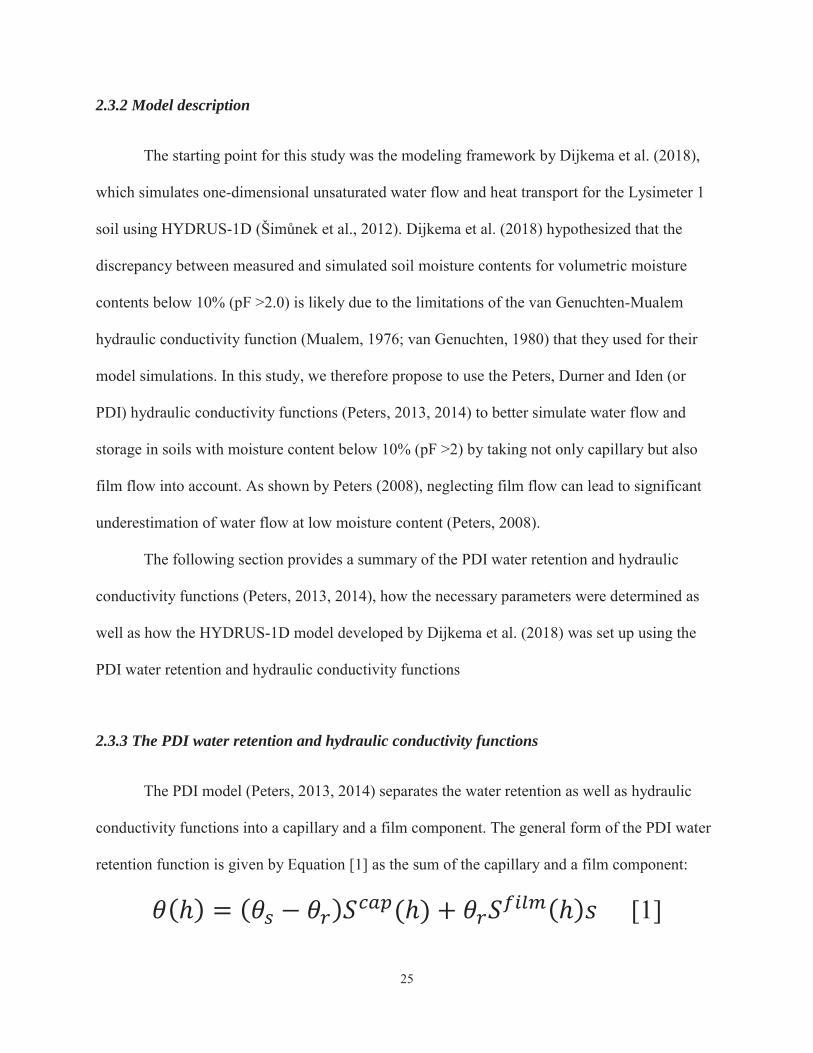
2.3.3 The PDI water retention and hydraulic conductivity functions ........................... 25
2.3.4 Laboratory characterization of the PDI soil water retention and hydraulic
conductivity functions ...................................................................................................... 29
2.3.5 Model setup, initial and boundary conditions ....................................................... 31
2.3.6 Model validation ..................................................................................................... 31
2.4 RESULTS AND DISCUSSION ............................................................................................. 32
2.5 CONCLUSIONS ........................................................................................................... 40
2.6 REFERENCES .................................................................................................................. 42

xi
CHAPTER 3 ........................................................................................................................... 45
3.1 SUMMARY ................................................................................................................... 45
3.2 INTRODUCTION ........................................................................................................ 47
3.3 MATERIALS AND METHODS ................................................................................. 48
3.3.1 Study site, soil and lysimeter design ....................................................................... 48
3.3.2 Near surface soil moisture measurements using TPHP ....................................... 50
3.3.3 Model setup, initial and boundary conditions ....................................................... 53
3.3.4 Laboratory characterization of the soil water retention and hydraulic conductivity
functions ........................................................................................................................... 54
3.3.5 Comparison of soil moisture measurements and simulations .............................. 55
3.4 RESULTS AND DISCUSSION ................................................................................... 56
3.5 CONCLUSIONS ........................................................................................................... 66
3.6 REFERENCES ............................................................................................................. 67
CHAPTER 4 ........................................................................................................................... 69
4.1 SUMMARY ................................................................................................................... 69
4.2 INTRODUCTION ........................................................................................................ 70
4.3 MATERIALS AND METHODS ................................................................................. 73
4.3.1 Experimental site .................................................................................................... 73
4.3.2 Soil Sampling .......................................................................................................... 74
4.3.3 Soil laboratory analysis .......................................................................................... 77
4.3.4 Monitoring atmospheric and soil moisture conditions ......................................... 78
4.3.5 Model setup, initial and boundary conditions ....................................................... 79
4.4 RESULTS AND DISCUSSION ................................................................................... 82
4.4.1 Soil properties ......................................................................................................... 82
4.4.2 In-situ soil moisture content monitoring ............................................................... 86
4.4.3 Soil moisture modeling ........................................................................................... 88
4.5 CONCLUSIONS ......................................................................................................... 100
4.6 REFERENCES ........................................................................................................... 101
CHAPTER 5 ......................................................................................................................... 104

xii
APPENDIX A. : SOIL SAMPLING AT THE DRI “SOLAR 1” PV FACILITY IN LAS
VEGAS .................................................................................................................. 110
APPENDIX B. : VAN GENUCHTEN FOR SOILS OF VARIOUS SOLAR
INSTALLATIONS IN NEVADA ....................................................................................... 113
CURRICULUM VITAE ...................................................................................................... 115

xiii
LIST OF TABLES
Table 2-1:Parameters of the lysimeter 1 soil layer at 10 cm depth for the BVG (Dijkema et
al., 2018) and the PDI (Peters, 2013) water retention and hydraulic conductivity
functions ............................................................................................................................... 30
Table 2-2 :Model performance comparison ............................................................................. 35
Table 3-1 Parameters of the for the PDI water retention and hydraulic conductivity
functions (Peters, 2013) for the Lysimeter 1 soil layer at 10 cm depth ........................... 55
Table 3-2 Model Performance (RMSE) .................................................................................... 65
Table 4-1 Soil texture and organic matter content of the soil of borehole #1 ........................ 82
Table 4-2 Soil bulk density determined from gravimetric and volumetric moisture contents
using Equation [1] ................................................................................................................ 83
Table 4-3 Parameters for the water retention and hydraulic conductivity functions
according to Peters (2013) for the Solar 1 soil. ................................................................. 85
Table B-1 values of some solar power plants in Nevada .................................................... 113

xiv
LIST OF FIGURES
Figure 2-1:Water retention functions of three separate measurements (left) and hydraulic
conductivity functions (right). Black circles indicate measurements, blue lines the
corresponding BVG functions from Dijkema et al. (2018) and pink lines the PDI
functions (Peters, 2013). ...................................................................................................... 33
Figure 2-2: Measured compared to simulated volumetric water content of Lysimeter 1 at
10 cm depth for the time period from Day 320 to Day 365. The black line shows
measured data, the pink line simulated data using the BVG and the blue line using the
PDI hydraulic functions. The green line is indcating 10% volumetric moisture content.
............................................................................................................................................... 35
Figure 2-3 Measured compared to simulated water content of Lysimeter 1 at 10 cm depth
for the time period from Day 1 to Day 125. The black line shows measured data, the
blue and pink lines simulations using the BVG and PDI hydraulic functions
respectively. .......................................................................................................................... 37
Figure 2-4 Measured and simulated cumulative surface fluxes during the calibration (top)
and validation period (bottom) of Dijkema et al. (2018). The black line represents the
flux measurements, the blue lines the flux simulations with the BVG and pink lines the
flux simulations with the PDI hydraulic functions. .......................................................... 39
Figure 3-1 TPHP sensor schematic (modified from Chief et al., 2009). ................................. 51
Figure 3-2 Schematic of the array of four TPHPs ................................................................... 52
Figure 3-3 Schematic (Figure 3-2) and placement (Figure 3-3) of the array of the four
TPHP probes in the near-surface soil of Lysimeter 1 (Chief et al., 2009) ...................... 52

xv
Figure 3-4 Soil moisture content of Lysimeter 1 between 12 mm and 100 mm depth from
May 1st to October 1st ,2019. Moisture contents were read with TPHP sensors except
for 10 cm depth were TDR probes were used. .................................................................. 58
Figure 3-5 Soil moisture content of Lysimeter 1 between 18 mm and 100 mm depth from
August 19th to September 30th, 2012. Moisture contents were read with TPHPs sensors
except for 100 mm depth where TDR probes were used. ................................................ 61
Figure 3-6 Soil moisture content measurements and simulations of Lysimeter 1 between
18mm and 100mm depth from February 16th to July 9th, 2017. Moisture contents were
read with TPHPs sensors except for 100 mm depth where TDR probes were used. .... 63
Figure 4-1 A conceptual model showing deep infiltration along the drip lines, shallow
infiltration between rows and no infiltration underneath a row of solar PV panels (Luo
et al., 2016). ........................................................................................................................... 71
Figure 4-2 Solar 1 PV facility on DRI’s Las Vegas campus. Solar 1 has 204 PV panels and a
nominal output of 52 kW (Luo et al., 2016)....................................................................... 73
Figure 4-3 Schematic of Solar 1 experimental site with TDR probe to monitor soil moisture
contents at 5 cm, 15 cm and 25 cm depth between PV panel rows (borehole #1), at one
of the drip lines (borehole #2) and underneath the panels (borehole #3). ...................... 74
Figure 4-4 Soil profile at borehole #1 located in between the panels. Pretty soft soil from 0
cm to 10cm depth, overlying a harder layer between 10 cm and 25 cm, overlying a
much softer layer between 25 cm and 35 cm depth. Sampling depth was limited to 35
cm by the length of the drill bit. ......................................................................................... 76
Figure 4-5 Model domain and precipitation pattern (upper flux boundary condition during
rain events) for the FE simulations (modified from Luo et al., 2016). ............................ 80

xvi
Figure 4-6 Measured (open circles) water retention curve (left) and hydraulic conductivity
function (right) of the soil at Solar 1. Lines represent fitted water retention and
hydraulic conductivity functions used to determine the parameters for the model by
Peters (2013) ......................................................................................................................... 84
Figure 4-7 Volumetric moisture content as a function of time at 5 cm, 15 cm and 25 cm
depth for the Solar 1 soil (a) between rows of solar panels, (b) in the drip line and (c)
underneath the solar panels. Note that the three locations roughly correspond to
boreholes 1, 2 and 3 (Figure 4-3) were also the soil sampling was performed. .............. 87
Figure 4-8 Measured vs. simulated soil moisture content at 5cm, 15cm and 25 cm depth in
the soil between the solar arrays. The simulations were run for a winter storm that
lasts from January 1st to March 31th, 2018. Assuming actual evaporation (ET) being
equal to 5%, 10% and 20% respectively of potential evapotranspiration (PET). ........ 89
Figure 4-9 Measured vs. simulated soil moisture content at 5cm and 25 cm depth in the soil
at the dripline. ...................................................................................................................... 90
Figure 4-10 Measured vs. simulated soil moisture content at 15cm and 25 cm depth in the
soil under the solar panel. ................................................................................................... 91
Figure 4-11 Measured vs. simulated soil moisture content at 5 cm, 15 cm and 25 cm depth
in the soil between the solar arrays. The simulations were run for a series of summer
storm events occurring from July 1st to September 30st, 2018 and assuming actual
evaporation (ET) being equal to 3% of potential evapotranspiration (PET). ............... 93
Figure 4-12 Measured vs. simulated soil moisture content at 5 cm and 25 cm depth in the
soil of the dripline. ............................................................................................................... 94

xvii
Figure 4-13 Measured vs. simulated soil moisture content at 15cm and 25 cm depth in the
soil under the solar panel. ................................................................................................... 95
Figure 4-14 Moisture redistribution in the Solar 1 soil before, during and after the January
9th ,2018 storm event. ........................................................................................................... 97
Figure 4-15 Moisture redistribution in the Solar 1 soil before, during and after the March
10th ,2018 storm event. ......................................................................................................... 98
Figure A-1 Ryan operating the power drill at borehole #2 ................................................... 111
Figure A-2 Yuan vacuuming out borehole #1 between the panels ....................................... 112
Figure A-3 Yuan, Ryan and Brian sampling soil from 0-14” depth at borehole #2 ........... 112
1
CHAPTER 1
DISSERTATION OVERVIEW
1.1 INTRODUCTION
Desert soils cover about one third of the Earth’s land surface (Hare, 1985) of which
between 15 and 25% are located in arid climates with average annual precipitation less than 250
mm. In the context of agriculture, desert soils and how to cultivate them were important since
ancient times (Hillel 1991, 1998). Outside of the realm of agricultural, however, the interest in
desert soils was limited until recently, when soils became increasingly recognized as important
parts of desert environments with impacts on climate, desert ecosystems and human
developments, as well as a resource for various, non-agricultural human activities. For example,
Desert soils are known to affect cloud and dust formation as well as CO2 fluxes, impacting
climate at a global scale (Austin et al., 2004; Huxman et al., 2004; Morgan et al., 2004;
Bhattachan et al., 2012). Desert soils also provide services to fragile ecosystems with a flora and
fauna adapted to limited water resources (Nichols, 1994; Kidron and Gutschick, 2013; Devitt et
al. ,2011; Moreno-de las Heras et al., 2016; Dong et al.,2007; Darby et al., 2011; Belnap et al.,
2004). With increasing population in desert environments, some of the fastest growing cities in
the world are located in arid areas (e.g. Kenny & Juracek, 2012), desert soils became
increasingly important for various human activities such as living, recreation, waste disposal, and
energy generation (Dregne, 1991; D’Odorico et al. ,2013). Expanding human developments in
desert environments are facing issues such as dust, flooding and erosion that are all directly

2
related to soils (Rosenfeld et al. ,2001; Okin et al., 2004; Capon & Brock, 2006; Belnap et
al.,1998). Desert environments, however, also offer opportunities e.g. for renewable energy
generating by large-scale solar facilities. Minimizing their impact on the fragile desert
environment (including its soils) is important for the solar industry to keep solar energy
environmentally friendly (First Solar, 2016).
Despite this increasing interest in desert soils, there still is little known about their basic
physical properties and processes, in particularly of the near-surface soil (top centimeters to
decimeters). The near-surface soil governs infiltration, storage and evapotranspiration of the
sparse precipitation, hosts most of the biologic activity, and also controls runoff, soil erosion as
well as the emission of dust. Existing studies primarily focused on deep infiltration of water to
assess groundwater recharge or contaminant transport to assess the viability of desert soils for
waste disposal (Gee et al., 1994; Andraski, 1997; Scanlon et al.,2005; Andraski et al.,2014;
National Security Technologies, 2015). Only recently, the focus shifted more towards near-
surface soil. For example, in 2008 a lysimeter facility was established in Boulder City, NV, to
study the moisture dynamics of near-surface arid soils (Chief et al., 2009, Koonce, 2016). The
Scaling Environmental Processes in Heterogeneous Arid Soil (or SEPHAS;
https://www.dri.edu/sephas) facility consist of three weighing lysimeters of 226 cm diameter and
300 cm depth filled with desert soil from the nearby Eldorado Valley in combination with an
Eddy Covariance micrometeorological station. Soil moisture and temperature within the
lysimeters are monitored hourly at various depths from 1 to 250 cm. The lysimeter scales are
able to detect changes in lysimeter mass equivalent to 0.1 mm of precipitation or evaporation.
Koonce (2016) analyzed precipitation, evaporation and soil moisture data from the three
lysimeters recorded from 2008 to 2012. He found that soil moisture dynamics by infiltration,

3
redistribution and evaporation is most pronounced in the top 25 cm of the soil profile with the
biggest moisture content changes occurring in the top 5 cm. Dijkema et al. (2018) employed the
data by Koonce (2016) to develop a process-based soil physics model in HYDRUS-1D (Šimůnek
et al., 2016) with the goal to simulate water distribution within the lysimeter soil as a function of
precipitation and evaporation. The model by Dijkema et al. (2018) is able to simulate water
movement within the lysimeter soil. In particular in parts of the soil profile where the soil is
moist, i.e. the volumetric soil moisture content exceedes 8% (<pF 2.0). The model’s capabilities
to capture water movement in the soil at moisture content below 8% (>pF 2.0) were limited. In
particular with respect to infiltration into initially dry soil with moisture content below 8% and
evaporation from the soil once the soil surface moisture content drops below 8%. Dijkema et al.
(2018) concluded that this is likely due to the limitations of the van Genuchten-Mualem
hydraulic conductivity function (Mualem, 1976; van Genuchten, 1980) to simulate water flow in
dry soil. The data by Koonce (2016) show that in times between storms (which is a large fraction
of the year in an arid environment), moisture content within the top 25 cm of the lysimeter soil
can drop below 5% and as low as 1% to 2% within the top 5 cm of the soil profile.
To capture water infiltration into dry soil as well as evaporation from dry soil surfaces,
we need a soil hydraulic function (or maybe functions) that captures water flow in dry soils
better than the current van Genuchten-Mualem function (Mualem, 1976; van Genuchten, 1980).
Alternative soil hydraulic functions have been proposed by Peters et al. (2015), Rudivanto et al.,
(2015) as well as Tuller and Or (2001) but so far have not been tested or applied to arid soils.
Therefore, the overarching goal of this study was to explore and test alternative hydraulic
functions that could improve our capabilities to model water redistribution in dry soil to better

4
understand and simulate water infiltration into and evaporation off arid soils and, eventually, the
moisture dynamics of near-surface arid soils.
1.2 LITERATURE REVIEW
A comprehensive review by Koonce (2016) showed that there are relatively few studies
that have provided insight into the moisture dynamics of arid soils. They are primarily driven by
research on groundwater recharge and waste disposal. A similar review on the role of the
antecedent moisture content of desert soils on flood prediction yielded only few studies. The
studies by Koonce (2016) and Dijkema et al. (2018) are the first ones that specifically address
the moisture dynamics of near-surface arid soil. The following sections provide an overview on
the state of knowledge with respect to the moisture dynamics of soils in desert environments.
1.2.1 Lysimeter studies around the world
Weighing lysimeters are important tools for characterizing near-surface water movement
processes. In the field of agriculture, some weighing lysimeter facilities have been built in desert
environment to estimate crop water use for irrigation scheduling (Evett et al., 2009; Scanchez et
al., 2011). Evapotranspiration is always a big concern for studying hydrologic cycles in
vegetated arid soils (Sammis, 1981; Young et al., 1996; Lan, et al., 2004). Usually, a comparison
of two lysimeters with different arid conditions (Levitt et al., 1996; Tomlinson, 1996) can be
used to provide support for water dynamics model testing or evapotranspiration studies. Some
other atmospheric phenomenon may also cause curiosity of researchers, like the formation of
dew in desert (Heusinkveld et al., 2006).

5
1.2.2 Antecedent moisture content and runoff prediction
Knowledge of water dynamics in arid soil has its significance in other applications than
groundwater recharge and waste disposal. For example, despite the low amounts of annual
precipitation, deserts are prone to surface runoff and flooding due to the high intensity and short
duration of desert rain storms as well as the specific soil conditions, in particular the low
antecedent moisture content (AMC). The Curve Number (CN), commonly used method to
estimate runoff, is heavily reliant on choosing the right AMC of the near surface soil. If having a
better estimation of the AMC, we will be able to predict more accurate runoff amount after
rainfall for flooding prevention purpose.
For example, Wang et al. (2008) evaluated rainfall infiltration and redistribution
processes under the natural rainfall events in semiarid desert environment with a bare soil
situation and a vegetated soil situation. They addressed the relationship between the rainfall
intensity and infiltration rate and found a linear correlation with the infiltration rate equating
80% of the rainfall intensity. In addition, the study addressed the effect of antecedent soil water
content on the rainfall infiltration depth. Wang et al. (2008) found that infiltration was
significantly reduced, both the cumulative infiltration and the infiltration depth, with the increase
in the antecedent soil moisture content. Similarly, work by Hardie et al. (2011) investigated the
effect of antecedent soil moisture on preferential flow properties in a series of texture-contrast
soils. The searchers found that under dry soil conditions, water moves more rapidly to depths of
around 1.0 m. Results also indicate that by maintaining soils at high antecedent moisture content,
infiltration can largely be restricted to near surface soils. These findings agree with Wang et al.

6
(2008), but conflict with some other studies, which demonstrate that as antecedent soil moisture
increases, the pore networks become more connected resulting in greater and more rapid
subsurface flow (McDonnell, 1990; Sidle et al., 1995). Gvirtzman et al. (2008) monitored spatial
and temporal variations in water content along unsaturated zone to understand the process of
water infiltration through stratified loess sediments down to a large depth (20 m below ground
surface). The observed water content results were simulated using a numerical code following
the van Genuchten-Mualem model (Mualem, 1976; van Genuchten, 1980). Those simulations
showed that the propagation of the wetting front is hampered by the extremely low values of the
surrounding unsaturated hydraulic conductivity, leading to the increasing of moisture content
within the onion-shaped wetted zone up to full saturation.
With recent progress in determining surface moisture content by remote sensing,
estimating AMC became easier. However, current remote sensing technics still rely on a very
basic understanding of the soil moisture profile in near-surface soils. In fact, the remotely sensed
soil moisture signal strongly depends on the soil moisture profile of the top few centimeters
(depending on the soil texture and moisture content), which is largely unknown unless directly
measured or obtained by soils physical simulations run after a storm event.
1.2.3 Infiltration, redistribution and evaporation of water in near-surface arid soil
Koonce (2016) analyzed precipitation, evaporation and soil moisture data from the three
SEPHAS weighing lysimeters recorded over a four-year time period from 2008 to 2012. He
found that between 69% and 90% of annual precipitation evaporated back into the atmosphere
during the course of a water year (October through September). Water years with large amounts
of winter precipitation (water years 2010 and 2011) yielded higher water storage compared to
7
winters with lower amounts of winter precipitation (water years 2009 and 2012). Throughout
spring, summer and autumn, most of the recorded precipitation evaporated back into the
atmosphere, even after storms with sizeable amounts of total precipitation. As for the soil
moisture profile, two precipitation thresholds were found. The first threshold ranged between
0.5- and 2-mm total precipitation, representing the smallest amount of precipitation to cause a
change in soil moisture content > 0.01 m3 m-3 at 2.4 cm depth. This range depended on season,
antecedent soil moisture, and the amount of time between previous and successive events. Events
with less than 1-2 mm total precipitation have little to no impact on moisture content below the
immediate soil surface (top inch or so). With respect to soil water storage, water from storms
with 1-2 mm total precipitation evaporates within a day, and do not have an impact on long-term
soil water storage. The second precipitation threshold could be defined as the smallest amount of
total precipitation needed to change soil moisture content at 25 cm depth by > 0.01 m3 m-3. Only
14 out of the 180 events (or sequence of events) changed soil moisture content at 25 cm depth or
deeper. The 10 largest precipitation events (with respect to total amount of precipitation) were
analyzed in more detail. Following all 10 events, soil moisture at 25 cm increased by 0.01m3 m-3
or more with total precipitation, intensity, and duration ranging between 13.2-41.6 mm, 0.6-12.3
mm hr-1, and 1.5-52 hours, respectively. During the four-year study period, only 7 events (or
sequences of events) changed soil moisture content down to 50 cm depth or deeper. Koonce
(2016) concluded that most of the moisture dynamics (infiltration, redistribution and
evaporation) occurs within the top 25 cm. Precipitation that remains above 25 cm tends to
evaporate within the course of a water year whereas water the infiltrates below 25 cm seem to
remain in the soil and fosters further infiltration during and after storm events. The findings by
Koonce (2016) were confirmed by Lehmann et al. (2019) who analyzed decade-long water flux

8
and moisture content time series from the SEPHAS lysimeters using the surface evaporation (or
SEC) model developed by Or and Lehmann (2019). They found that between 2008 and 2018
only 10 rain events led to a net mass gain for the lysimeters and that the soil moisture is affected
by evaporation as deep as 50 cm.
Koonce (2016) also tested a recently developed, process-based evaporation model by
Shokri et al. (2009) and Or et al. (2013) to simulate evaporation from the weighing lysimeter
soil. The model focusses on water-vapor diffusion controlled (or Stage III) evaporation (Idso et
al., 1974) and calculates Stage III evaporation rates based on soil texture, total porosity and an
initial moisture content profile as input parameters. Simulations of the evaporation rates using
readily available soil physical properties agreed well with two out of the three events that were
analyzed (evaporation rate RMSEs of 0.093- and 0.141-mm d-1, respectively). For the third
event, simulations systematically underestimated measured evaporation rates (RMSE of 0.181
mm d-1). The latter was likely due to considerable differences between the moisture profile in the
near-surface lysimeter soil compared to the simplified moisture profile that is assumed by the
model. Monte-Carlo simulations showed that total porosity and difference in soil moisture
content above and below the secondary drying front are the model’s most sensitive parameters.
Since total porosity can be determined rather accurately, improving on characterizing the near-
surface soil moisture profile would likely improve evaporation predictions for arid soil using the
model by Shokri et al. (2009) and Or et al. (2013).
Based on the data by Koonce (2016), Dijkema et al. (2018) developed a process-based
model within HYDRUS-1D (Šimůnek et al., 2016) to describe the moisture dynamics within the
lysimeter soil as a function of water fluxes through the soil surface. A modified van Genuchten
function was introduced to capture the dry end of the soil water retention curve. A scaling

9
method was proposed to account for variabilities in water retention to account for the differences
in bulk density within the lysimeter soil profile. The model was calibrated and validated using
hourly soil moisture, temperature and mass data from the SEPHAS weighing lysimeters (Chief et
al., 2009). Dijkema et al. (2018) found that their model very well simulated infiltration into moist
soil as well as moisture redistribution within the soil. The model also described well the early
stages of evaporation (i.e., Stage I and parts of Stage II evaporation) when the evaporative
demand at the soil surface rather than soil hydraulic properties control evaporation (Idso et al.,
1974). The model, however, consistently underestimated Stage II and Stage III evaporation when
evaporation is controlled by the soil hydraulic properties. Dijkema et al. (2018) identified two
potential causes that contributed to this discrepancy. First, Richard’s equation does not permit
hydraulic discontinuity and cannot handle vapor diffusion-limited water transfer from a
subsurface drying (evaporation) front upward to the soil surface. The forced continuity of liquid
water presents all the way to the soil surface requires unrealistic equilibration between an
extremely dry but continuous thread of liquid water and vapor. Vapor flow that occurs under
such conditions is likely to underestimate Stage III evaporation. Secondly, the classic van
Genuchten-Mualem hydraulic conductivity function used in the HYDRUS-1D code likely
underestimates water flow rates at the dry end of the soil water retention curve. Based on these
results, Dijkeman et al. (2018) concluded that more work is needed to delineate the relative
contributions of these two shortcomings and to correct for their effects in order to get more
accurate Stage II and Stage III evaporation estimations.
1.3 OBJECTIVE, HYPOTHESES AND APPROACH

10
The overarching of this study is to explore and test alternative hydraulic functions that
improve our capability to model water redistribution arid soil from near-saturation to, ideally,
air-dry conditions. Such functions will help us to better simulate water infiltration into and
evaporation off arid soils and, eventually, to improve our understanding of the moisture
dynamics of near-surface desert soils. I started with the alternative hydraulic functions proposed
by Peters (2013) and tested the following two hypotheses:
1. Replacing the van Genuchten-Mualem (van Genuchten, 1980) with the Peters (2013)
hydraulic functions in the modeling framework by Dijkema et al. (2018) will improve the
accuracy of soil moisture content predictions for the SEPHAS Lysimeter 1 soil,
especially for moisture contents below 8% volumetric water content (or >pF 2).
2. The model by Dijkema et al. (2018) in combination with Peters (2013) allows to capture
the soil moisture dynamics of the top 50 mm of a bare, near-surface soil profile due to
precipitation and evaporation.
To test these hypotheses, I simulated soil moisture redistribution in the top 100 mm of the
Lysimeter 1 soil for several wetting and drying events employing the model by Dijkema et al.
(2018) but with the Peters (2013) hydraulic functions. Soil water retention and hydraulic
conductivity functions needed for the model simulations I measured in the laboratory using a
combination of evaporation experiments employing HYPROP and WP4-C devices (Meter Inc.).
I then compared modeled with measured moisture content data of the soil profile from 12 mm to
54 mm depth (at 6 mm intervals) using Triple-Point-Heat-dissipation Probes (TPHPs) and 100
mm depth using Time Domain Reflectometry (or TDR) probes. The near-surface soil moisture
dataset from 12 mm to 54 mm depth is unique and has not been considered in any previous

11
studies. The model by Dijkema et al. (2018) with the hydraulic functions by Peters (2013) was
then used to simulate the impact of an array of photovoltaic (PV) solar panels on the water
distribution in the soil underneath and between rows of PV panels as a function of precipitation
and evaporation to assess the impact solar arrays on the hydrology within a solar PV facility.
The following three chapters address the abovementioned objective, hypotheses and
approach in more details with Chapter 2 focusing on improving the model by Dijkema et al.
(2018) by replacing the van Genuchten-Mualem hydraulic functions with the ones by Peters
(2013), hereafter referred to as Luo et al. (2019a)and Chapter 3 testing the Luo et al. (2019a)
model on a soil moisture dataset from the top 50 mm of Lysimeter 1. Chapter 4 then describes an
application of the Luo et al. (2019a) model to simulate the impact of an array of PV solar panels
on the water distribution in the soil underneath and between rows of PV panels as a function of
precipitation and evaporation to assess the impact solar arrays on the hydrology within a solar
PV facility. Note that Chapters 2, 3 and 4 were prepared as individual journal articles with
Chapter 2 intended for submission to the Vadose Zone Journal, Chapter 3 to the Soil Science
Society of America Journal and Chapter 4 to Case Studies in the Environment.
1.4 REFERENCES
Andraski, B. J. (1997). Soil-water movement under natural-site and waste-site conditions: A multiple-year field study in the Mojave Desert, Nevada. Water Resources Research 33, 1901-1916.
Andraski, B. J., Jackson, W. A., Welborn, T. L., Bohlke, J. K., Sevanthi, R., and Stonestrom, D. A. (2014). Soil, Plant, and Terrain Effects on Natural Perchlorate Distribution in a Desert Landscape. Journal of Environmental Quality 43, 980-994.
Austin, A. T., Yahdjian, L., Stark, J. M., Belnap, J., Porporato, A., Norton, U., Ravetta, D. A., and Schaeffer, S. M. (2004). Water pulses and biogeochemical cycles in arid and semiarid ecosystems. Oecologia 141, 221-235.

12
Belnap, J., Phillips, S. L., and Miller, M. E., (2004), Response of desert
biological soil crusts to alterations in precipitation frequency: Oecologia, v. 141, p. 306-316.
Capon, S. J., & Brock, M. A. (2006). Flooding, soil seed bank dynamics and vegetation resilience of a hydrologically variable desert floodplain. Freshwater Biology, 51(2), 206–223.
Bhattachan, A., D'Odorico, P., Baddock, M. C., Zobeck, T. M., Okin, G. S., and Cassar, N. (2012). The Southern Kalahari: a potential new dust source in the Southern Hemisphere? Environmental Research Letters 7, 024001.
Campbell, G. S., J. D. Jungbauer, Jr., W. R. Bidlake, and R. D. Hungerford. (1994). Predicting the effect of temperature on soil thermal conductivity. Soil Sci. 158:307–313.
Campbell, G. S. and J. M. Norman. (1997). An introduction to environmental biophysics. Springer-Verlag, New York.
Capon, S. J., & Brock, M. A. (2006). Flooding, soil seed bank dynamics and vegetation resilience of a hydrologically variable desert floodplain. Freshwater Biology, 51(2), 206–223.
Chief, K., M.H. Young, B.F. Lyles, J. Healey, J. Koonce, E. Knight, E. Johnson, J. Mon, M. Berli, M. Menon, and G. Dana (2009). Scaling environmental processes in heterogeneous arid soils: construction of large weighing lysimeter facility: Division of Hydrologic Sciences, Desert Research Institute Pub. No. 41249.
Chung, S. O., and Horton, R. (1987). Soil Heat and Water-Flow with a Partial Surface Mulch. Water Resources Research 23, 2175-2186.
Devitt, D. A., Fenstermaker, L. F., Young, M. H., Conrad, B., Baghzouz, M., and Bird, B. M. (2011). Evapotranspiration of mixed shrub communities in phreatophytic zones of the Great Basin region of Nevada (USA). Ecohydrology 4, 807-822.
de Vries, D. A., (1952). A nonstationary method for determining thermal conductivity of soil in situ. Soil Sci. 73:83–89.
Dijkema, J., J. Koonce, R. Shillito, T. Ghezzehei, M. Berli, M. Van der Ploeg and M. T. Van Genuchten (2018). "Water Distribution in an Arid Zone Soil: Numerical analysis of data from a large weighing lysimeter" Vadose Zone Journal: 17, 170035, DOI: 10.2136/vzj2017.01.0035.

13
Dregne, H., Kassas, M., and Rozanov, B. (1991). A new assessment of the world status of desertification. Desertification Control Bulletin 20, 6-18.
D'Odorico, P., Bhattachan, A., Davis, K. F., Ravi, S., and Runyan, C. W. (2013). Global desertification: Drivers and feedbacks. Advances in Water Resources 51, 326-344.
Dong H, JA Rech, H Jiang, H Sun, BJ Buck. (2007). Endolithic cyanobacteria in soil gypsum: occurrences in Atacama (Chile), Mojave (USA), and Al-Jafr Basin (Jordan) Deserts. J Geophys Res – Biogeosci, 112, G02030,doi:02010.01029/02006JG000385.
Darby, B., Housman, D. C., Neher, D., and Belnap, J., (2011), Few apparent short-term effects of elevated soil temperature and increased frequency of summer precipitation on the abundance and taxonomic diversity of desert soil micro- and meso-fauna: Soil Biology and Biochemistry, v. 43, p. 1474-1481.
Durner, W. (1994). Hydraulic conductivity estimation for soil with heterogeneous pore structure. Water Resour. Res. 30, 211-223.
First Solar (2016). First Solar Responsible Land Use White Paper. First Solar, Inc., Tempe, AZ.
Garcia, C.A., B.J. Andraski, D.A. Stonestrom, C.A. Cooper, J. Simunek and S.W. Wheatcraft.
(2011). Interacting Vegetative and Thermal Contributions to Water Movement in Desert Soil.
Vadose Zone Journal 10: 552-564.
Gee, G. W., Wierenga, P. J., Andraski, B. J., Young, M. H., Fayer, M. J., and Rockhold, M. L. (1994). Variations in Water-Balance and Recharge Potential at 3 Western Desert Sites. Soil Science Society of America Journal 58, 63-72.
Gvirtzman, H., Shalev, E., Dahan, O., & Hatzor, Y. H. (2008). Large-scale infiltration experiments into unsaturated stratified loess sediments: Monitoring and modeling. Journal of Hydrology, 349(1–2), 214–229.
Hare, F. K. (1985). Climate Variations, Drought and Desertification, World Meteorological Organization,, Geneva, Switzerland.

14
Heusinkveld, B. G., Berkowicz, S. M., Jacobs, A. F. G., Holtslag, A. a. M., & Hillen, W. C. a. M. (2006). An Automated Microlysimeter to Study Dew Formation and Evaporation in Arid and Semiarid Regions. Journal of Hydrometeorology, 7(4), 825–832.
Huxman, T. E., Snyder, K. A., Tissue, D., Leffler, A. J., Ogle, K., Pockman, W. T., Sandquist, D. R., Potts, D. L., and Schwinning, S. (2004). Precipitation pulses and carbon fluxes in semiarid and arid ecosystems. Oecologia 141, 254-268.
Hardie, M. A., Cotching, W. E., Doyle, R. B., Holz, G., Lisson, S., & Mattern, K. (2011). Effect of antecedent soil moisture on preferential flow in a texture-contrast soil. Journal of Hydrology, 398(3–4), 191–201.
Hopmans, J. W., Simunek, J., and Bristow, K. L. (2002). Indirect estimation of soil thermal properties and water flux using heat pulse probe measurements: Geometry and dispersion effects. Water Resources Research 38.
Hillel, D. J. (1991). Out of the Earth : Civilization and the Life of the Soil, The Free Press, New York, NY.
Hillel, D. (1998). Environmental Soil Physics, 1/Ed. Academic Press, San Diego.
Idso, S. B., Reginato, R. J., Jackson, R. D., Kimball, B. A., and Nakayama, F. S. (1974). The three stages of drying of a field soil. Soil Science Society America Journal 38, 831-837.
Kidron, G. J., and Gutschick, V. P. (2013). Soil moisture correlates with shrub-grass association in the Chihuahuan Desert. Catena 107, 71-79.
Kenny, J. F., and Juracek, K., E. (2012). Description of 2005–10 domestic water use for selecting U.S. cities and guidance for estimating domestic water use. U.S. Geological Survey, Washington, D.C.
Kluitenberg, G.J., J.M. Ham, and K.L. Bristow. (1993). Error analysis of the heat pulse method for measuring soil volumetric heat capacity. Soil Sci. Soc. Am. J. 57:1444–1451.
Koonce, J.E. (2016). Water balance and moisture dynamics of an arid and semi-arid soil: a weighing lysimeter and field study. Ph.D., University of Nevada Las Vegas. 168p.

15
Laliberte, G. E., Corey, A. T., and Brooks, R. H. (1966). "Properties of Unsaturated Porous Media." Colorado State University, Fort Collins, Colorado.
Lan, S., Kang, E.-S., Zhang, J.-G., & Berndtsson, R. (2004). Evapotranspiration of Artemisia ordosica Vegetation in Stabilized Arid Desert Dune in Shapotou, China. Arid Land Research and Management, 18(1), 63–76.
Lehmann, P., Berli, M., Koonce, J.E. and Or, D. (2019) Surface evaporation in arid regions: Insights from lysimeter decadal record and global application of a surface evaporation capacitor (SEC) model. Geophysical Research Letters 46(16), 9648-9657
Levitt, G. (1996). An Arid Zone Lysimeter Facility for Performance Assessment and Closure. Investigations at the Nevada Test Site.
Morgan, J. A., Pataki, D. E., Korner, C., Clark, H., Del Grosso, S. J., Grunzweig, J. M., Knapp, A. K., Mosier, A. R., Newton, P. C. D., Niklaus, P. A., Nippert, J. B., Nowak, R. S., Parton, W. J., Polley, H. W., and Shaw, M. R. (2004). Water relations in grassland and desert ecosystems exposed to elevated atmospheric CO2. Oecologia 140, 11-25.
Mori, Y., J.W. Hopmans, A.P. Mortensen, and G.J. Kluitenberg. (2003). Multi-functional heat pulse probe for the simultaneous measurement of soil water content, solute concentration, and heat transport parameters. Vadose Zone J. 2:561–571.
Mualem, Y. (1976). A new model for predicting the hydraulic conductivity of unsaturated porous media. Water Resource Research 12, 513–522.
McDonnell, J.J.(1990). A rationale for old water discharge through macropores in a steep, humid catchment. Water Resources Research 26 (11), 2821–2832.
Moldrup, P., T. Olesen, J. Gamst, P. Schjonning, T. Yamaguchi and D.E. Rolston. (2000). Predicting the gas diffusion coefficient in repacked soil: Water-induced linear reduction model. Soil Science Society of America Journal 64: 1588-1594.
Moreno-de las Heras, M., Turnbull, L., and Wainwright, J. (2016). Seed-bank structure and plant-recruitment conditions regulate the dynamics of a grassland-shrubland Chihuahuan ecotone. Ecology 97, 2303-2318.
Nichols, W.D. (1994). Groundwater discharge by phreatophytes shrubs in the Great-Basin as

16
related to depth to groundwater. Water Resources Research 30: 3265-3274.
NSTEC (2015). Nevada National Security Site 2014 Waste Management Monitoring Report Area 3 and Area 5 Radioactive Waste Management Sites. US Department of Energy, Oak Ridge, TN.
Okin, G. S., Mahowald, N., Chadwick, O. A., & Artaxo, P. (2004). Impact of desert dust on the biogeochemistry of phosphorus in terrestrial ecosystems. Global Biogeochemical Cycles, 18(2).
Or, D. and Lehmann, P. (2019) Surface evaporative capacitance: How soil type and rainfall characteristics affect global scale surface evaporation. Water Resources Research 55(1), 519–539
Or, D., P. Lehmann, E. Shahraeeni and N. Shokri. (2013). Advances in Soil Evaporation Physics- A Review. Vadose Zone Journal 12.
Peters, A., Iden, S. C., & Durner, W. (2015). Revisiting the simplified evaporation method: Identification of hydraulic functions considering vapor, film and corner flow. Journal of Hydrology, 527, 531–542.
Philip, J. R., and de Vries, D. A. (1957). Moisture movement in porous materials under temperature gradients. American Geophysical Union Transactions 38, 222-232.
Rosenfeld, D., Rudich, Y., & Lahav, R. (2001). Desert dust suppressing precipitation: a possible desertification feedback loop. Proceedings of the National Academy of Sciences of the United States of America, 98(11), 5975–80.
Rudiyanto, Sakai, M., van Genuchten, M. T., Alazba, A. A., Setiawan, B. I., & Minasny, B. (2015). A complete soil hydraulic model accounting for capillary and adsorptive water retention, capillary and filmconductivity, and hysteresis. Water Resources Research, 51, 8757–8772.
Sammis, T. W. (1981). Lysimeter for measuring arid-zone evapotranspiration. Journal of Hydrology, 49, 385–394.
Sanchez, C. A., & Sciences, E. (2011). Determination of Evapotranspiration ( ET ) for Desert Durum Wheat using Weighing Lysimeters in the Lower Colorado River Region.

17
Scanlon, B. R., Levitt, D. G., Reedy, R. C., Keese, K. E., and Sully, M. J. (2005). Ecological controls on water-cycle response to climate variability in deserts. Proceedings of the National Academy of Sciences of the United States of America 102, 6033-6038.
Simunek, J., van Genuchten, M. T., and Sejna, M. (2016). Recent Developments and Applications of the HYDRUS Computer Software Packages. Vadose Zone Journal 15.
Sidle, R.C. et al. (1995). Seasonal hydrologic response at various spatial scales in a small forested catchment, Hitachi Ohta, Japan. Journal of Hydrology 168 (1–4), 227–250.
Simunek, J., Genuchten, M. Van, & Sejna, M. (2012). HYDRUS: Model use, calibration, and validation. Transactions of the ASABE, 55(1987), 1261–1274.
Saito, H., Simunek, J., and Mohanty, B. P. (2006). Numerical analysis of coupled water, vapor, and heat transport in the vadose zone. Vadose Zone Journal 5, 784-800.
Shokri, N., P. Lehmann and D. Or. (2009). Critical evaluation of enhancement factors for vapor transport through unsaturated porous media. Water Resources Research 45.
Shokri, N. and D. Or. (2011). What determines drying rates at the onset of diffusion controlled stage-2 evaporation from porous media? Water Resources Research 47.
Tomlinson, B. S. a. (1996). Weighing-Lysimeter Evapotranspiration for Two Sparse-Canopy Sites in Eastern Washington.
Tuller, M., Or, D., and Dudley, L. M. (1999). Adsorption and capillary condensation in porous media: Liquid retention and interfacial configurations in angular pores. Water Resources Research 35, 1949-1964.
Tuller, M., & Or, D. (2001). Hydraulic conductivity of variably saturated porous media: Film and corner flow in angular porous media. Water Resources Research, 37 (5)(5), 1257–1276.
Wang, X. P., Cui, Y., Pan, Y. X., Li, X. R., Yu, Z., & Young, M. H. (2008). Effects of rainfall characteristics on infiltration and redistribution patterns in revegetation-stabilized desert ecosystems. Journal of Hydrology, 358(1–2), 134–143.

18
Young, M.H, P.J, Wierenga., and C.F, Mancino. (1996). Large weighing lysimeters for water and deep percolation studies. Soil Science, 161(8), 491–501.
Young, M.H., G.S. Campbell and J. Yin. (2008). Correcting dual-probe heat-pulse readings for changes in ambient temperature. Vadose Zone Journal 7: 22-30.
19
CHAPTER 2
MODELING NEAR-SURFACE WATER REDISTRIBUTION IN A DESERT
SOIL
Prepared for submission to Vadose Zone Journal by
Yuan Luo, Teamrat A. Ghezzehei, Zhongbo Yu and Markus Berli
2.1 SUMMARY
Desert soils cover about one third of the Earth’s land surface. Despite their rather large
extent, however, our understanding of and ability to simulate the moisture dynamics of near-
surface desert soils (top centimeters to a few meters) remain limited. A recent study by Dijkema
et al. (2018) introduced a modeling framework to simulate water redistribution in a bare, near-
surface desert soil. Their model was able to capture accurately captured water redistribution
under infiltration as well as evaporation conditions. For the latter, however, only when the soil
was relatively moist (volumetric moisture content >10%, matric head <pF 2). For dryer soil
conditions, the model consistently underestimated evaporative fluxes and, subsequently,
overestimated soil moisture content. The goal of this study was to expand the modeling
framework by Dijkema et al. (2018) by using the Peters-Durner-Iden (or PDI) water retention
and hydraulic conductivity functions (Peters, 2014), that are able to capture capillary as well as
film flow, instead of the bimodal van Genuchten Mualem (or BVG) water retention and

20
hydraulic conductivity functions (van Genuchten, 1980) to simulate water redistribution at lower
soil water content. We found that the PDI water retention functions (Peters 2014) better represent
the measured water retention curves than the BVG water retention functions used by Dijkema et
al. (2018). In particular for the critical range of volumetric moisture contents between 5% and
10% (saturation degrees between 16% and 32%, and matric heads between pF 2 and 4). The
BVG water retention functions predicted higher suctions (lower matric heads) than the PDI
functions for volumetric moisture contents in the range from 5% to10% likely leading to an
underestimation of the hydraulic conductivity values and water fluxes in the soil in the range
from 5% to 10%. Interestingly, the BVG and PDI hydraulic conductivity functions were not
noticeably different within the range between pF 2 and 3 where most of the HYPROP
measurements were available. For pF values higher than 3, however, the PDI functions predicted
higher hydraulic conductivity values than the BVG functions. Therefore, the hypothesis put
forward by Dijkema et al. (2018) that including film flow may improve model predictions could
be confirmed for pF >3. For pF values between 2 and 3, however, is probably rather the
difference between BVG and PDI water retention functions than hydraulic conductivity
functions that led to the improved soil moisture simulations.
In conclusions, the HYDRUS-1D model developed by Dijkema et al. (2018) can
accurately predict moisture content values as low as 6% (or 19% saturation and pF 3.8) when
using the PDI instead of the BVG water retention and hydraulic conductivity functions, provided
good quality water retention and hydraulic conductivity data are available to parametrize the PDI
functions. Further research is needed to explore whether the PDI model could capture water
redistribution at volumetric soil moisture contents even lower than 6% (pF >3.8), maybe as low
as 2%, which would correspond to the Lysimeter 1 soil at air-dry conditions.

21
2.2 INTRODUCTION
Desert soils cover about one third of the Earth’s land surface (Hare, 1985) of which
between 15 and 25% are located in arid climates with average annual precipitation less than 250
mm. Despite the rather large extent of desert soils, our understanding of their basic hydraulic
processes and properties is still rather limited. In particularly with respect to the near-surface (top
centimeters to decimeters of the soil profile), which governs infiltration, redistribution and
evapotranspiration of the sparse precipitation, hosts most of the biologic activity, and also
controls runoff, erosion and the emission of dust (Nannipieri et al.,2003, Bradford et al.,1987).
In a recent study, Dijkema et al. (2018) developed a modeling framework with in
HYDRUS-1D (Šimůnek et al., 2012) to simulate water redistribution in a desert soil as a
function of precipitation and evaporation using experimental data from one of the SEPHAS
weighing lysimeters (Chief et al., 2009; Koonce, 2016). The process-based model by Dijkema et
al. (2018) accurately captured near-surface water redistribution under infiltration as well as
evaporation conditions. For the latter, however, only when the soil was relatively moist
(volumetric moisture content >10%, matric head <pF 2). For dryer soil conditions, however, the
model consistently underestimated evaporative fluxes and, subsequently, overestimated soil
moisture content. Dijkema et al. (2018) hypothesized that the van Genuchten-Mualem hydraulic
conductivity function (Mualem, 1976; van Genuchten, 1980), which they used for their model,
may not be ideal for drier soil conditions since it does not take film flow into account and an
alternative hydraulic conductivity model might be needed that can capture liquid water flow for
drier soil conditions. Peters (2013) developed a process-based approach that can account for
capillary and film flow and developed it into the Peter-Durner-Iden (or PDI) model, which has
the potential to simulate water fluxes in unsaturated soils from water saturated to air-dry

22
conditions (Peters, 2014). The aim of this study was to test the hypothesis put forward by
Dijkema et al. (2018) and simulate soil moisture distributions of the SEPHAS weighing
lysimeter with the PDI hydraulic conductivity functions (Peters, 2014) and then compare the
PDI-based simulations with the simulations using the van Genuchten-Mualem hydraulic
conductivity function as well as measurements from the lysimeter soil. A key step for this study
was to measure the water retention and hydraulic conductivity functions of the Lysimeter 1 soil
using HYPROP and W4C devices (METER Inc.) since both the van Genuchten-Mualem as well
as the PDI functions heavily depend on the accuracy of the water retention and hydraulic
conductivity data to determine the necessary soil physical parameters. The overarching goal was
to improve the HYDRUS-1D model developed by Dijkema et al. (2018) to simulate the near-
surface water redistribution in a desert soils for a wider range of soil moisture content.

23
2.3 MATERIALS AND METHODS
2.3.1 Study site and soil
This study was carried out with data from the SEPHAS weighing lysimeter facility,
which was already described by Chief et al. (2009) and Koonce (2016) and its data used by
Dijkema et al. (2018). In this paper, we therefore only provide a brief overview of the study site,
lysimeter design as well as the soil involved and refer to Chief et al. (2009), Koonce (2016) and
Dijkema et al. (2018) for further details.
The SEPHAS weighing lysimeter facility (https://www.dri.edu/sephas) is located in
Boulder City, Nevada (35.96°N, 114.85°W), approximately 40 km southeast of Las Vegas,
Nevada, in the Mojave Desert. The lysimeters are at an elevation of 768 m and receive an
average annual precipitation 141 mm, with average daily temperatures ranging from 8.1 °C in
January to 31.7 °C in July (Western Regional Climate Center, 2017). The lysimeter soil stems
from the nearby Eldorado Valley study site and developed from volcanic parent material (mainly
Andesite and Rhyolite) that was deposited on a south-facing, shallow-sloped alluvial fan (0-15%
slope angle) from the McCullough and Highland Ranges (Chief et al., 2009). The soil has been
classified as a sandy-skeletal, mixed, thermic Typic Torriorthents of the Arizo series (Soil
Survey Division Staff, 1993). The vegetation in Eldorado Valley consists primarily of creosote
bush (Larrea tridentata) and white bursage (Ambrosia dumosa) is typical for the Mojave Desert.
The SEPHAS lysimeters are cylindrical, stainless steel tanks with a diameter of 226 cm
and a depth of 300 cm, which are placed on truck scales and housed underground in individual
rooms accessible by a tunnel (Dijkema et al., 2018; Chief et al., 2009). The scales have a
resolution of 450 g and can detect changes in lysimeter mass equivalent to a water column of 0.1
mm height. The lysimeter tanks were filled with soil from bottom to top in individual lifts

24
(between 2 and 22 cm lift thickness), with each individual lift being repacked as closely as
possible to the bulk densities measured at the Eldorado Valley study site. For this study, only the
data from Lysimeter 1 were used. Lysimeter 1 has a homogenous texture profile with a fine
fraction (particle diameter < 2 mm) consisting of 93.0 % sand, 5.5 % silt, and 1.5 % clay and an
average gravel content of 18.9 % by mass. Bulk densities of the lysimeter soil profile range from
1,442 to 1,798 kg m-3, yielding total porosity to range from 0.24 to 0.31 (as calculated based on
an average measured particle density of 2,479 kg m-3 and gravel content of 18.9%). Since its
installation in 2008, Lysimeter 1 have been kept free of vegetation. Volumetric moisture contents
were measured at depths of 10, 25, 50, 75, 100, 150, 200, and 250 cm using time-domain
reflectometry (TDR) probes (model CS605, Campbell Scientific Inc., Logan, UT). The
arithmetic means of four soil water content measurements were calculated for each depth and the
averages were used for comparison with the various calculations. Hourly precipitation and
evaporation rates were calculated from lysimeter mass readings taken at 15 minutes intervals.
Concurrently, precipitation rates were monitored using a tipping bucket rain gage (Model
TE525WS-L, Campbell Scientific, Inc., Logan, UT) located approximately 30 m west of
Lysimeter 1. The rain gage provided precipitation data at 30-minute intervals. Similar to
Dijkema et al. (2018), this study focused on Lysimeter 1 data from October 1, 2011, at 00:00
hours to September 30, 2012, at 23:00 hours, which resulted in 8,784 hourly measurements.
25
2.3.2 Model description
The starting point for this study was the modeling framework by Dijkema et al. (2018),
which simulates one-dimensional unsaturated water flow and heat transport for the Lysimeter 1
soil using HYDRUS-1D (Šimůnek et al., 2012). Dijkema et al. (2018) hypothesized that the
discrepancy between measured and simulated soil moisture contents for volumetric moisture
contents below 10% (pF >2.0) is likely due to the limitations of the van Genuchten-Mualem
hydraulic conductivity function (Mualem, 1976; van Genuchten, 1980) that they used for their
model simulations. In this study, we therefore propose to use the Peters, Durner and Iden (or
PDI) hydraulic conductivity functions (Peters, 2013, 2014) to better simulate water flow and
storage in soils with moisture content below 10% (pF >2) by taking not only capillary but also
film flow into account. As shown by Peters (2008), neglecting film flow can lead to significant
underestimation of water flow at low moisture content (Peters, 2008).
The following section provides a summary of the PDI water retention and hydraulic
conductivity functions (Peters, 2013, 2014), how the necessary parameters were determined as
well as how the HYDRUS-1D model developed by Dijkema et al. (2018) was set up using the
PDI water retention and hydraulic conductivity functions
2.3.3 The PDI water retention and hydraulic conductivity functions
The PDI model (Peters, 2013, 2014) separates the water retention as well as hydraulic
conductivity functions into a capillary and a film component. The general form of the PDI water
retention function is given by Equation [1] as the sum of the capillary and a film component: (ℎ) = ( − ) (ℎ) + (ℎ) [1]

26
where is the volumetric water content, h the matric head, s is the volumetric water content at
saturated, and r, the residual water content (i.e. the volumetric water content at the lowest
matric head). Scap and Sfilm are the saturation degrees of the capillary and film components,
respectively, of the water retention function, which are both functions of the matric head, h.
According to Peters (2014), the saturation degree of the capillary component, Scap, can be
described as (ℎ) = ( ) [2]
with Γ(h), an effective capillary function and Γ0 = Γ(h0) the effective capillary function Γ(h) for
the matric head h0 = -107 cm (equivalent to oven-dry conditions or 0% volumetric moisture
content)
According to Peters (2013), Γ(h) can be a unimodal capillary function such as van
Genuchten (1980), a pore size distribution function such as Kosugi(1996), or a bimodal capillary
function such as proposed by Durner (1994). In this study, we used van Genuchten (1980) as the
effective capillary function, Γ(h) Γ(ℎ) = 11+( ℎ) [3]
with, n and the empirical van Genuchten parameters (van Genuchten 1980) and m = 1-1/n.
For the saturation degree of the film component of the water retention function, Sfilm, Peters
(2014) gives: ( ) = 1 + − + ln 1 + [4]

27
where = log10(-ℎ) is the pF value for the matric head h, and x = log10(-ℎ ) the pF value for the
matric head at air entry, ha. According to Peters (2013), the matric head at air entry can be
estimated as ha = -1, with the van Genuchten parameter. 0 can range from 5 to 7 depending
on the residual moisture content with and 0 = 5.5- 6.3 for air-dry 20-80% relative humidity
and 0 = 7 for oven-dry conditions. The shape parameter, b, in equations [4] can be calculated
by: = 0.1 + . 1 − − [5]
With n the van Genuchten parameter (van Genuchten, 1980), s the volumetric water content at
saturation and r the residual water content (Peters, 2013).
Similar to the water retention function given by Equation [1], Peters (2013) also introduced a
model for the hydraulic conductivity function as the sum of a capillary and a film flow
component: = + [6]
Peters’ (2013) hydraulic conductivity function also includes an additional component for water
vapor flow. In this study, however, we focused only on the liquid water flow part of the model
because vapor flow is already included in the model by Dijkema et al. (2018) using the approach
by Philip and DeVries (1957). Peters (2013) defined and according to Equations [7] = ( );

28
= [7]
where and are the capillary and film conductivities, respectively, at
saturation. = ω and = (1 − ω) , with ω a empirical weighing factor for the
film flow contribution to the hydraulic conductivity (Peters 2013). and refer to the
relative hydraulic conductivities due to capillary and film flow, which are functions of effective
saturation of the capillary (Scap, Equation 2) and film (Sfilm, Equation 4) components of the water
retention functions.
With van Genuchten (1980) as the effective capillary function for Equation [3] Peters
(2013) gives the following relative hydraulic conductivity function for capillary flow: = ( ) 1 − // [8]
with the tortuosity of the pore system, usually assumed to be 0.5 (Mualem, 1976), m = 1-1/n
and n the van Genuchten parameter (van Genuchten, 1980). The relative hydraulic conductivity
for film flow is given by Peters (2013) as:
= [9]
where is an empirical parameter [usually assumed to be -1.5 according to Tokunaga (2009) and
Peters (2013)] and h is the matric head at air entry.

29
2.3.4 Laboratory characterization of the PDI soil water retention and hydraulic conductivity functions
For their study, Dijkema et al. (2018) had only limited water retention and hydraulic
conductivity data available. For the water retention curve, for example, in-situ soil moisture
content and matric head measurements from Lysimeter 1 but only for a limited range of pF
values from 2 to about 4. Also, besides saturated hydraulic conductivity, no other hydraulic
conductivity measurements were available. Therefore, one goal of this study was to obtain a
more robust water retention and hydraulic conductivity dataset for the Lysimeter 1 soil.
Particularly for the range of matric heads between -100 cm and -1000 cm (pF 2 and 3), which
Dijkema et al. (2018) have identified as critical for their water redistribution simulations.
So for this study, soil water retention and hydraulic conductivity functions were
determined by the evaporation method using a HYPROP device (Meter Environment Inc.) and
absorption method using a WP4C dew-point potentiometer (Meter Environment Inc.). The
HYPROP device is particularly suited to measure water retention and hydraulic conductivity
functions in the range between pF 2 and 3. The WP4C, in combination with an analytical balance
(Mettler Toledo MS 104 TS) was used to measure water potentials and corresponding water
content of the soil at the dry end of the water retention curve (pF 3.3 - 6.3). Following the
protocol developed by Kriste and Durner (2018) we were able to obtain a complete water
retention curve for Lysimeter 1 soil ranging from pF 0 to pF 6.3.
For the HYPROP and WP4C measurements, only the fine fraction (<2mm particle
diameter) of Lysimeter 1 soil could be used. Lysimeter 1 soil, however, has an average gravel
content (particle diameters larger than 2 mm) of 18.9% by mass. Also, Dijkema et al. (2018)
noted the significant influence the bulk density profile of the lysimeter soil has on its hydraulic
properties. Therefore, the influence of gravel content and bulk density on the soil hydraulic

30
properties were taken into account by the scaling method proposed by Vogel et al. (1991) and
further developed by Dijkema et al. (2018). Based on the HYPROP and WP4C measured water
retention and hydraulic conductivity functions for Lysimeter 1 soil (Figure 2-1), and the scaling
by Vogel et al. (1991) and Dijkema et al. (2018), we determined the PDI parameters saturated,
s, and residual volumetric water contents, r, the van Genuchten parameters n and , the matric
head at air-entry, ha, the matric head for oven-dry condition, h0, and the and the weighing factor
for the film flow contribution to the hydraulic conductivity, ω, for the Lysimeter 1 soil. The
parameters for the soil at 10 cm depth are shown in Table 2-1 together with the corresponding
parameters for the BVG model using in Dijkema et al. (2018).
Table 2-1:Parameters of the Lysimeter 1 soil layer at 10 cm depth for the BVG (Dijkema et al., 2018) and the PDI (Peters, 2013) water retention and hydraulic
conductivity functions
Parameters for BVG hydraulic functions (Dijkema et al., 2018)
Parameters for PDI hydraulic functions (Peters, 2013)
PARAMETER VALUE UNIT PARAMETER VALUE UNIT
Saturated water content, θs
0.292 - Saturated water content, θs
0.31 -
Residual water content, θr
0 - Residual water content, θr
0.02 -
BVG α1 (coarse sub-curve)
1.57 × 10⁻² [1/cm] van Genuchten α
1.21 × 10-
2 [1/cm]
BVG n1 (coarse sub-curve) 2.571 - van Genuchten n 3.2 -
BVG α2 (fine sub-curve)
1 × 10⁻⁴ [1/cm] h0 -106.8 [cm]
BVG n2 (fine sub-curve) 1.35 -
Slope of film conductivity function
on log-log scale, a -1.5 -
Weighing factor for the bimodal retention
curve, w 0.245 -
Weight factor for film flow contribution to the
saturated hydraulic conductivity, ω
6 × 10⁻⁴ -
Saturated hydraulic conductivity, Ks
2.0 [cm/h] Saturated hydraulic conductivity, Ks
0.43 [cm/h]
*The Ks for the PDI model was fitted by using HYPROP-FIT (Pertassek et al., 2015).

31
2.3.5 Model setup, initial and boundary conditions
The same HYDRUS-1D model as in Dijkema et al. (2018) was set up with 600 elements
of 0.5 cm length to simulate the 300 cm deep soil profile of Lysimeter 1. The only difference was
that the BVG were replaced by the PDI soil water retention and hydraulic conductivity functions
as given in Equations [1]-[9]. In particular, the same total soil bulk density profile was used as in
Dijkema et al (2018, Fig. 2). Also similar to Dijkema et al. (2018), the initial soil moisture
profile was determined from the hourly soil moisture content values measured by the TDR
probes in Lysimeter 1 placed between 10 and 250 cm depth. Since there are no sensors at the
surface (0 cm) and bottom (300 cm) of the lysimeter, the top and bottom sensor values were
extended to the top and bottom of the model domain, respectively.
The water flux boundary condition at the lysimeter surface were calculated from the
hourly changes in lysimeter mass, since the soil in Lysimeter 1 was bare and all the mass
changes were assumed to be either due to precipitation or evaporation. The bottom boundary was
set as “free drainage” conditions, i.e. assuming a unit hydraulic gradient at the bottom of the soil
column. Lateral flow and lysimeter wall effects are neglected in this one-dimension model.
2.3.6 Model validation
Soil moisture data from Day 0 to Day 125 and Day 320 to Day 365 of the 2012 water
year (October 1st ,2011 to September 30th ,2012) were used to validate the model calculations.
These were the same two soil moisture content data sets already used by Dijkema et al. (2018),
which allowed for a direct comparison of the simulation results using the PDI and BVG

32
hydraulic functions in the Dijkema et al. (2018) model. The model’s goodness of fit was
expressed in terms of the mean error (ME) and root mean square error (RMSE) calculated by the
following equations [10] and [11]: = ∑ [ − ] [10]
= ∑ [ − ] [11]
where si and oi represent the simulated and observed water contents of sample i, respectively,
and N is the number of measurements.
2.4 RESULTS AND DISCUSSION
In a first step, soil water retention and hydraulic conductivity functions were measured
for the Lysimeter 1 soil. Figure 2-1 (left) shows three measured water retention and Figure 2-1
(right) three measured hydraulic conductivity functions (round symbols) with the corresponding
fitted BVG (Dijkema et al., 2018, blue lines) and PDI (Peters, 2014, red line) water retention and
hydraulic conductivity functions using Petrassek et al. (2015). The PDI water retention functions
represent the measured values better than the BVG water retention functions. The BVG functions
overestimate the measured matric heads quite a bit particularly in the range between pF 2 and pF
4 (or volumetric moisture content between 5% and 10%). This difference between BVG and PDI
water retention functions likely causes the model by Dijkema et al. (2018) to underestimate the
hydraulic conductivity for the range of 5% to10% volumetric moisture content, which would
explain the lower simulated compared to measured evaporative flux found by Dijkema et al.
(2018, Fig. 6 and Fig.11).

33
Figure 2-1:Water retention functions of three separate measurements (left) and hydraulic conductivity functions (right). Black circles indicate measurements,

34
blue lines the corresponding BVG functions from Dijkema et al. (2018) and pink lines the PDI functions (Peters, 2013).
It is interesting to note that the BVG and PDI hydraulic conductivity functions (Figure 2-
1, right) do not differ much from the measured hydraulic conductivity functions for the range
between pF2 and 3 where measurements were available. So, for the range of pF value between 2
and 3, it is more likely the water retention rather than the hydraulic conductivity function that
limits the Dijkema et al. (2018) model’s capability to simulate water redistribution in the soil.
Figure 2-2 (bottom) does show, however, that for pF values higher than 3, the PDI function
predicts higher hydraulic conductivity values than the BVG function for the same pF values.

35
Figure 2-2: Measured compared to simulated volumetric water content of Lysimeter 1 at 10 cm depth for the time period from Day 320 to Day 365. The black line shows
measured data, the pink line simulated data using the BVG and the blue line using the PDI hydraulic functions. The green line is indcating 10% volumetric
moisture content.
Figure 2-2 shows measured compared to simulated water contents at 10 cm depth of
Lysimeter 1 for the time period from Day 320 to Day 365, i.e. the calibration period from
Dijkema et al (2018). The black line shows measured data whereas the red and blue lines
simulated data using the BVG (Dijkema et al., 2018) and the PDI hydraulic functions (Peters,
2014). When using the PDI functions, the model captures the soil water dynamics of the three
simulated wetting and drying events better than when using the BVG functions, particularly for
volumetric moisture contents below 10% (green line), as also evident by the ME and RMSE
values for the respective simulations (Table 2-2). Figure 2-2 shows that simulations using the
PDI functions can capture soil moisture contents ranging from 8% to 28% corresponding to
saturation degrees from 26% to 90% (with a total porosity of 31% at 10 cm depth).
For additional validation as well as to test the model with the PDI functions for even
dryer soil conditions, we compared simulations with the PDI hydraulic functions and
measurements and simulations from the validation dataset used by Dijkema et al. (2018). The
results are shown in Figure 2-3 and confirm that the model using the PDI hydraulic functions
capture the water dynamics better than with the BVG hydraulic functions, reflected in the
corresponding ME and RMSE values for the two simulations (Table 2-2).
Table 2-2 :Model Performance Comparison
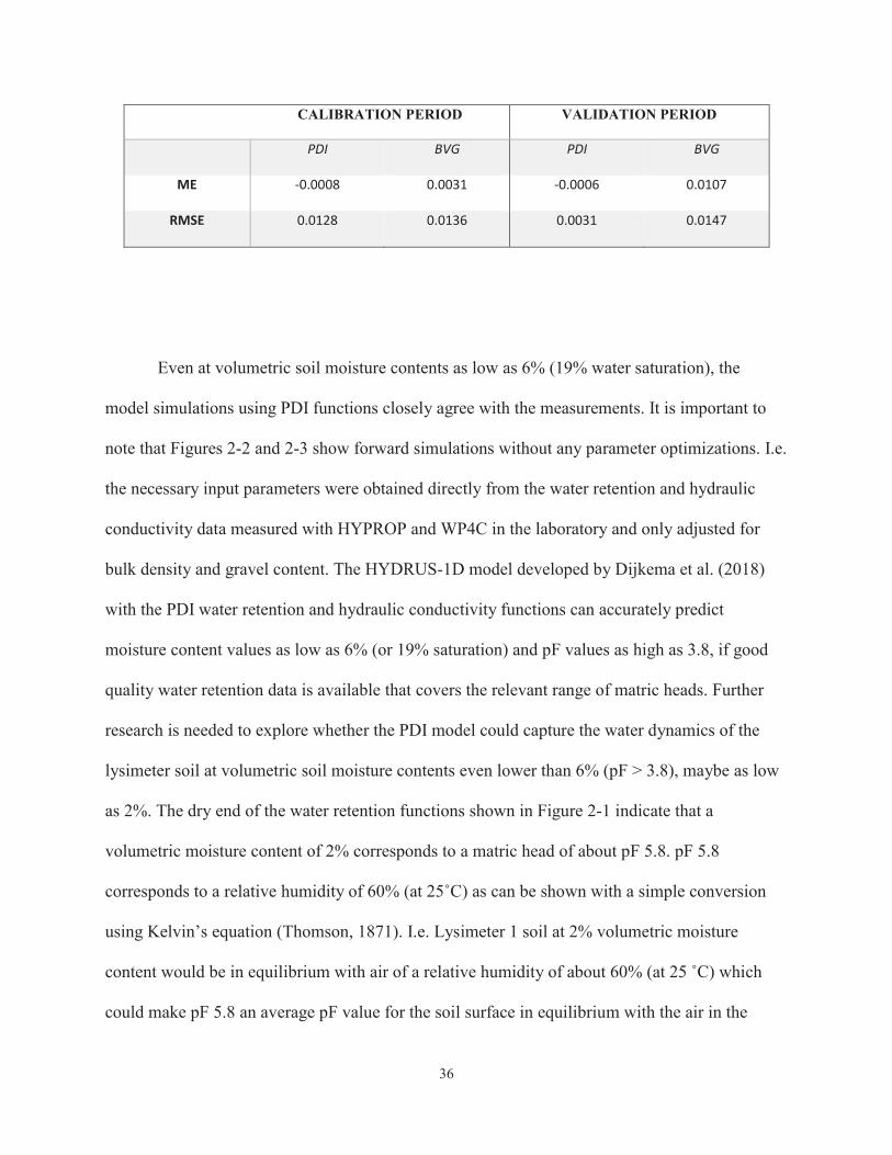
36
CALIBRATION PERIOD VALIDATION PERIOD
PDI BVG PDI BVG
ME -0.0008 0.0031 -0.0006 0.0107
RMSE 0.0128 0.0136 0.0031 0.0147
Even at volumetric soil moisture contents as low as 6% (19% water saturation), the
model simulations using PDI functions closely agree with the measurements. It is important to
note that Figures 2-2 and 2-3 show forward simulations without any parameter optimizations. I.e.
the necessary input parameters were obtained directly from the water retention and hydraulic
conductivity data measured with HYPROP and WP4C in the laboratory and only adjusted for
bulk density and gravel content. The HYDRUS-1D model developed by Dijkema et al. (2018)
with the PDI water retention and hydraulic conductivity functions can accurately predict
moisture content values as low as 6% (or 19% saturation) and pF values as high as 3.8, if good
quality water retention data is available that covers the relevant range of matric heads. Further
research is needed to explore whether the PDI model could capture the water dynamics of the
lysimeter soil at volumetric soil moisture contents even lower than 6% (pF > 3.8), maybe as low
as 2%. The dry end of the water retention functions shown in Figure 2-1 indicate that a
volumetric moisture content of 2% corresponds to a matric head of about pF 5.8. pF 5.8
corresponds to a relative humidity of 60% (at 25˚C) as can be shown with a simple conversion
using Kelvin’s equation (Thomson, 1871). I.e. Lysimeter 1 soil at 2% volumetric moisture
content would be in equilibrium with air of a relative humidity of about 60% (at 25 ˚C) which
could make pF 5.8 an average pF value for the soil surface in equilibrium with the air in the
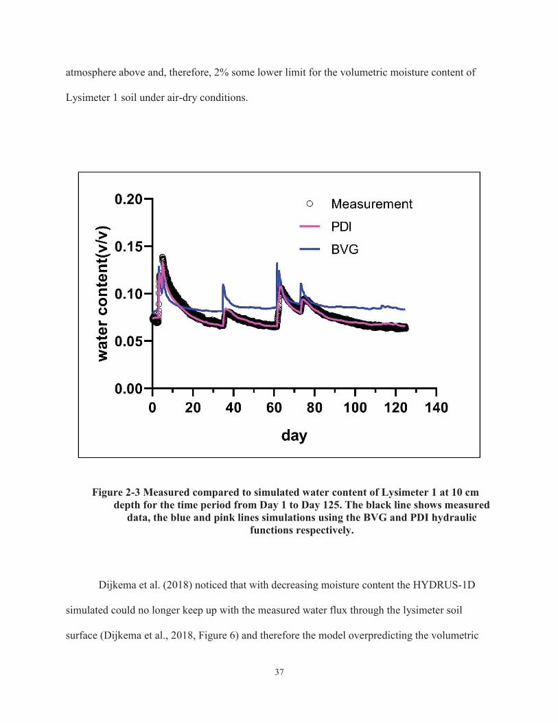
37
atmosphere above and, therefore, 2% some lower limit for the volumetric moisture content of
Lysimeter 1 soil under air-dry conditions.
Figure 2-3 Measured compared to simulated water content of Lysimeter 1 at 10 cm depth for the time period from Day 1 to Day 125. The black line shows measured
data, the blue and pink lines simulations using the BVG and PDI hydraulic functions respectively.
Dijkema et al. (2018) noticed that with decreasing moisture content the HYDRUS-1D
simulated could no longer keep up with the measured water flux through the lysimeter soil
surface (Dijkema et al., 2018, Figure 6) and therefore the model overpredicting the volumetric

38
moisture content of the soil, especially at 10 cm depth. We therefore run surface flux simulations
similar to the ones by Dikema et al. (2018) for the two soil moisture datasets used by Dikema et
al. (2018). Figure 2-4 shows the resulting flux simulation values in comparison to the measured
flux values for the same time periods. The simulations using PDI hydraulic functions can closely
simulate the measured flux values whereas the flux simulations with the BVG hydraulic
functions divert considerably.

39
Figure 2-4 Measured and simulated cumulative surface fluxes during the calibration (top) and validation period (bottom) of Dijkema et al. (2018). The black line
represents the flux measurements, the blue lines the flux simulations with the BVG and pink lines the flux simulations with the PDI hydraulic functions.

40
The better agreement of the flux simulations using the PDI functions compared to the
BVG functions could be explained with the lower matric heads predicted by PDI compared to
BVG functions and therefore higher hydraulic conductivity for the same volumetric water
content. I.e. for the same volumetric water content, the soil according to the PDI model remains
more hydraulically conductive than the soil according to the BVG model. The surface flux with
the PDI functions can therefore longer satisfy the evaporative demand than the surface flux
modelled with the BVG functions and can therefore simulate the drying out of the surface soil to
lower moisture contents.
2.5 CONCLUSIONS
The aim of this study was to improve the soil moisture redistribution model by Dijkema
et al. (2018) to capture soil moisture condition dryer then pF 2 or 32% water saturation during
evaporation. For that purpose, we replaced the bimodal van Genuchten-Mualem (BVG) water
retention and hydraulic conductivity functions in the model by Dijkema et al. (2018) with the
corresponding functions from the PDI model (Peters, 2014), which can capture the capillary as
well as film domain of moisture in the soil. We also determined water retention and hydraulic
conductivity functions of the Lysimeter 1 soil using a combination of HYPROP, WP4C and
falling head measurements.
We found that the PDI water retention functions (Peters, 2014) better represent the
measured water retention curves than the BVG water retention functions used by Dijkema et al.
(2018). In particular for the critical range of volumetric moisture contents between 5% and 10%

41
(saturation degrees between 16% and 32%, and matric heads between pF 2 and 4). The BVG
water retention functions predicted higher suctions (lower matric heads) than the PDI functions
for volumetric moisture contents in the range from 5% to 10% likely leading to an
underestimation of the hydraulic conductivity values and water fluxes in the soil in the range
from 5% to 10%. Interestingly, the BVG and PDI hydraulic conductivity functions were not
noticeably different within the range between pF 2 and 3 where most of the HYPROP
measurements were available. For pF values higher than 3, however, the PDI functions predicted
higher hydraulic conductivity values than the BVG functions. Therefore, the hypothesis put
forward by Dijkema et al. (2018) that including film flow may improve model predictions could
be confirmed for pF >3. For pF values between 2 and 3, however, is probably rather the
difference between BVG and PDI water retention than hydraulic conductivity functions that led
to the improved soil moisture simulations. A comparison between BVG-based and PDI-based
simulations for the soil moisture calibration and validation datasets used by Dijkema et al. (2018)
showed that the model by Dijkema et al. (2018) using PDI instead of BVG hydraulic functions
provided better soil moisture content predictions, especially for soil moisture levels less than
10% (lower than 32% saturation, higher than pF 2). In conclusion, replacing the BVG water
retention and hydraulic conductivity functions in the model by Dijkema et al. (2018) with the
corresponding functions from the PDI model (Peters 2014) considerably improved the ability of
the model by Dijkema et al. (2018) to capture soil moisture condition dryer then pF 2 or 32%
water saturation. Further research is needed to explore whether the PDI model could capture the
water dynamics of the lysimeter soil at volumetric soil moisture contents even lower than 6%
(pF > 3.8), maybe as low as 2%, which would correspond to air-dry conditions assuming an
average relative humidity of 60% (at 25˚C) for the air.

42
2.6 REFERENCES
Bradford J M, Ferris J E, Remley P A. Interrill Soil Erosion Processes: I. Effect of Surface Sealing on Infiltration, Runoff, and Soil Splash Detachment 1[J]. Soil Science Society of America Journal, 1987, 51(6): 1566-1571.
Chief, K., M.H. Young, B.F. Lyles, J. Healey, J. Koonce, E. Knight, E. Johnson, J. Mon, M. Berli, M. Menon, and G.D., 2009. Scaling Environmental Processes in Heterogeneous Arid Soils : Construction of Large Weighing Lysimeter Facility. Desert Research Institute, Las Vegas, NV.
Dijkema,J.; Koonce, J.E.; Shillito, R.M.; Ghezzehei, T.A.; Berli, M.; van der Ploeg, M.J.; van Genuchten, M.T., 2018. Water Distribution in an Arid Zone Soil: Numerical Analysis of Data from a Large Weighing Lysimeter. Vadose Zone Journal.
Durner, W., 1994. Hydraulic conductivity estimation for soils with heterogeneous pore structure. Water Resources Research 30, 211–223. https://doi.org/10.1029/93WR02676
Genuchten, M. Van, 1980. A closed-form equation for predicting the hydraulic conductivity of unsaturated soils. Soil science society of America journal.
Hare, F.K., 1985. Climate variations, drought and desertification. World Meteorol. Organ., Geneva, Switzerland.
Iden, S.C., Durner, W., 2014. Comment on “simple consistent models for water retention and hydraulic conductivity in the complete moisture range” by A. Peters. Water Resources Research 50, 7530–7534. https://doi.org/10.1002/2014WR015937
Koonce, J.E., 2016. Water Balance and Moisture Dynamics of an Arid and Semi-Arid Soil: A Weighing Lysimeter and Field Study. Ph.D. diss., Univ. of Nevada, Las Vegas.
Kosugi, K., 1996. Lognormal distribution model for unsaturated soil hydraulic properties 32, 2697–2703. Water Resources Research.

43
Kriste, Bjorn; Durner, W., 2018. Determining the soil water retention curve across the full moisture range by combing HYPROP and WP4C data. Poster at EGU.
Mualem, 1976. A new model for predicting the hydraulic conductivity of unsaturated porous media. Water Resources Research 12, 564–566. https://doi.org/10.1029/WR012i003p00564
Nannipieri P, Ascher J, Ceccherini M T, et al. Microbial diversity and soil functions[J]. European journal of soil science, 2003, 54(4): 655-670.
Peters A, Durner W. A simple model for describing hydraulic conductivity in unsaturated porous media accounting for film and capillary flow[J]. Water Resources Research, 2008, 44(11).
Peters, A., 2013. Simple consistent models for water retention and hydraulic conductivity in the complete moisture range. Water Resources Research 49, 6765–6780. https://doi.org/10.1002/wrcr.20548
Peters, A., 2014. Reply to comment by S. Iden and W. Durner on ‘“Simple consistent models for water retention and hydraulic conductivity in the complete moisture range.”’ Water Resources Research 2781–2786. https://doi.org/10.1002/2012WR013341.Reply
Pertassek, T., A. Peters and W. Durner (2015). HYPROP-FIT Software User’s Manual, V.3.0, METER Group AG, Mettlacher Str. 8, 81379 München, Germ any, 66 pp.
Reynolds, W.D. and D.E. Elrick. 2002. Falling head soil core (tank) method. In: J. H. Dane and G. C. Topp, editors, Methods of Soil Analysis. Soil Science Society of America Inc., Madison, WI. p. 809-817.
Philip, J.R. and D.A. de Vries. 1957. Moisture movement in porous materials under temperature gradients. American Geophysical Union Transactions 38: 222-232.
Simunek, J., Genuchten, M. Van, Sejna, M., 2012. HYDRUS: Model use, calibration, and validation. Transactions of the ASABE 55, 1261–1274.
Soil Survey Division Staff, 1993. Soil survey manual, Agriculture Handbook 18. USDA, Washington, DC.

44
Tokunaga, T.K., 2009. Hydraulic properties of adsorbed water films in unsaturated porous media. Water Resources Research 45, 1–9.
Thomson, W. 1871. On the equilibrium of vapour at the curved surface of liquid. Philosophical Magazine 42: 448-452.
Western Regional Climate Center, 2017. Cooperative Climatological Data Summaries. Western Regional Climate Control Center, Reno, NV.

45
CHAPTER 3
MOISTURE DYNAMICS IN A NEAR-SURFACE DESERT SOIL: MEASUREMENTS AND SIMULATIONS
Prepared for submission as a technical note to the Soil Science Society of America Journal (SSSAJ) by
Yuan Luo, John Healey, Michael H. Young, Teamrat A. Ghezzehei, and Markus Berli
3.1 SUMMARY
Desert soils cover about one third of the Earth’s land surface (Hare, 1985). Despite their
large extent and critical role for infiltration, redistribution and evapotranspiration of the sparse
precipitation. our understanding of desert soil hydraulic processes and properties is still rather
limited. In particularly with respect to the near-surface (top centimeters of the soil profile), which
hosts most of the biologic activity and controls runoff, erosion and the emission of dust
(Nannipieri et al.,2003; Bradford et al.,1987).
To improve our understanding of the moisture dynamics of a desert soil surface, the top 5
cm of the SEPHAS weighing lysimeters (https://www.dri.edu/sephas) were instrumented with an
array of Triple-Point-Heat-dissipation Probes (TPHP, East 30 Sensors, Inc., Pullman, WA).
These TPHPs allow to monitor volumetric soil moisture content and temperature near the soil
surface at 6 mm intervals from 0 mm to 54 mm on an hourly basis. The goal of this study was (a)
to monitor the soil moisture distribution of the bare, near-surface soil of Lysimeter 1 during
wetting-drying cycles and (b) to simulate these measured moisture distributions with the model
by Luo et al. (2019) using measured water fluxes from precipitation and evaporation as the
driving forces.

46
A soil moisture dataset was presented for the top 50 mm of the soil profile with 6 mm
spatial and 1-hour temporal resolution over a five-month period demonstrating the soil moisture
response to an initial precipitation event followed by almost five months of evaporation. The
dataset showed that only the top 20 mm of the soil dry out completely (i.e. reach a soil moisture
content below the detection limit of the TPHPs) whereas the soil moisture contents between 20
to 50 mm depths convert towards some equilibrium moisture contents between 3.5% and 5% (or
15% to 21% saturation, respectively). Soil moisture from precipitation in the top 50 mm of the
soil profile evaporates back into the atmosphere within one month or less with the soil moisture
spatial and temporal distribution of the top 50 mm hinting towards a two-step evaporation
mechanism as proposed by Shokri et al. (2008) and Or et al. (2013). We also compared measured
soil moisture time series for different depth with simulations using the model by Luo et al.
(2019) and found that the latter is able to pretty accurately forward-simulate soil moisture
redistribution in the top 100 mm of the soil profile for a wide range of soil moisture contents
from 15% to over 90% saturation using only independently determined soil physical parameters
as well as precipitation and evaporation as flux boundary conditions. Overall, the study shows
how the soil moisture distribution in the top 50 mm of a bare desert soil changes as a function of
precipitation and evaporation as well as confirms that the model by Luo et al. (2019) is able to
simulate the moisture dynamics of a bare, near-surface desert soil from near-saturation to about
twice the air-dry moisture content. Luo et al. (2019), however, was not able to simulate all the
soil moisture distribution features monitored with the TPHPs, indicating a more complicated
evaporation process than Luo et al. (2019) can capture.

47
3.2 INTRODUCTION
Desert soils cover about one third of the Earth’s land surface (Hare, 1985) of which
between 15 and 25% are in arid climates with average annual precipitation less than 250 mm.
Despite their large extent, our understanding of desert soil hydraulic processes and properties is
still rather limited. In particularly with respect to the near-surface (top centimeters of the soil
profile), which governs infiltration, redistribution and evapotranspiration of the sparse
precipitation, hosts most of the biologic activity, and also controls runoff, erosion and the
emission of dust (Nannipieri et al.,2003; Bradford et al.,1987).
To improve our understanding of the moisture dynamics of a desert soil surface, the top
5 cm of the SEPHAS weighing lysimeters (https://www.dri.edu/sephas) were instrumented with
an array of Triple-Point-Heat-dissipation Probes (TPHP, East 30 Sensors, Inc., Pullman, WA).
These TPHPs allow to monitor volumetric soil moisture content and temperature near the soil
surface at 6 mm intervals from 0 mm to 54 mm on an hourly basis.
In a recent study, Dijkema et al. (2018) developed a process-based soil physics model in
HYDRUS-1D (Šimůnek et al. 2012) to simulate water redistribution in a bare desert soil as a
function of precipitation and evaporation using experimental data from SEPHAS Lysimeter 1
(Chief et al., 2009; Koonce, 2016). Luo et al. (2019) improved the model by Dijkema et al.
(2018) to capture dryer soil conditions under evaporation by introducing soil hydraulic functions
of the Peters-Durner-Iden (or PDI) model (Peters, 2014). The model by Luo et al. (2019) is able
to simulate volumetric moisture contents as low as 6% (19% saturation or pF 3.5), which is a
considerable extension of the soil moisture range the model by Dijkema et al. (2018) is able to
simulate. The model by Luo et al. (2019) therefore has the potential to simulate the moisture

48
dynamics of a desert soil surface that experiences moisture content changes from air-dry to near-
water saturated and back to air-dry conditions.
The goal of this study was (a) to monitor the soil moisture distribution of the bare, near-
surface soil of Lysimeter 1 during wetting-drying cycles and (b) to simulate these measured
moisture distributions with the model by Luo et al. (2019) using measured water fluxes from
precipitation and evaporation as the driving forces.
3.3 MATERIALS AND METHODS
3.3.1 Study site, soil and lysimeter design
This study was carried out with data from the SEPHAS weighing lysimeter facility
(https://www.dri.edu/sephas) in Boulder City, Nevada (35.96°N, 114.85°W), approximately
40 km southeast of Las Vegas, Nevada. The SEPHAS weighing lysimeters have been described
in previous studies (Chief et al., 2009; Koonce, 2016; Dijkema et al., 2018). We therefore only
provide a brief overview of the study site, soil and lysimeter design.
The lysimeters are located in the Mojave Desert at an elevation of 768 m above sea level
and receive an average annual precipitation of 141 mm, with average daily temperatures ranging
from 8.1°C in January to 31.7°C in July (Western Regional Climate Center, 2017). The lysimeter
soil was collected from the nearby Eldorado Valley study site and developed from volcanic
parent material (mainly Andesite and Rhyolite) that was deposited on a south-facing, shallow-
sloped alluvial fan (0% to 15% slope angle) from the McCullough and Highland Ranges (Chief
et al., 2009). The soil has been classified as a sandy-skeletal, mixed, thermic Typic Torriorthents
of the Arizo series (Soil Survey Division Staff, 1993). The vegetation in Eldorado Valley
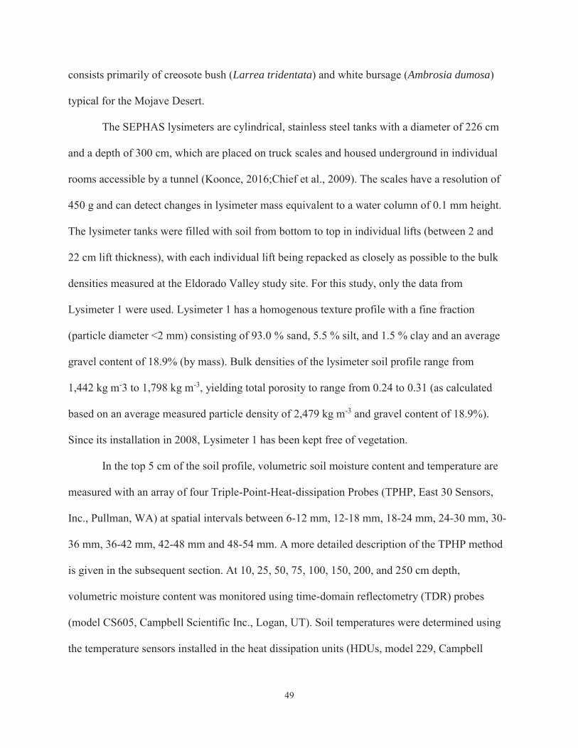
49
consists primarily of creosote bush (Larrea tridentata) and white bursage (Ambrosia dumosa)
typical for the Mojave Desert.
The SEPHAS lysimeters are cylindrical, stainless steel tanks with a diameter of 226 cm
and a depth of 300 cm, which are placed on truck scales and housed underground in individual
rooms accessible by a tunnel (Koonce, 2016;Chief et al., 2009). The scales have a resolution of
450 g and can detect changes in lysimeter mass equivalent to a water column of 0.1 mm height.
The lysimeter tanks were filled with soil from bottom to top in individual lifts (between 2 and
22 cm lift thickness), with each individual lift being repacked as closely as possible to the bulk
densities measured at the Eldorado Valley study site. For this study, only the data from
Lysimeter 1 were used. Lysimeter 1 has a homogenous texture profile with a fine fraction
(particle diameter <2 mm) consisting of 93.0 % sand, 5.5 % silt, and 1.5 % clay and an average
gravel content of 18.9% (by mass). Bulk densities of the lysimeter soil profile range from
1,442 kg m-3 to 1,798 kg m-3, yielding total porosity to range from 0.24 to 0.31 (as calculated
based on an average measured particle density of 2,479 kg m-3 and gravel content of 18.9%).
Since its installation in 2008, Lysimeter 1 has been kept free of vegetation.
In the top 5 cm of the soil profile, volumetric soil moisture content and temperature are
measured with an array of four Triple-Point-Heat-dissipation Probes (TPHP, East 30 Sensors,
Inc., Pullman, WA) at spatial intervals between 6-12 mm, 12-18 mm, 18-24 mm, 24-30 mm, 30-
36 mm, 36-42 mm, 42-48 mm and 48-54 mm. A more detailed description of the TPHP method
is given in the subsequent section. At 10, 25, 50, 75, 100, 150, 200, and 250 cm depth,
volumetric moisture content was monitored using time-domain reflectometry (TDR) probes
(model CS605, Campbell Scientific Inc., Logan, UT). Soil temperatures were determined using
the temperature sensors installed in the heat dissipation units (HDUs, model 229, Campbell

50
Scientific Inc., Logan, UT) used to measure soil water pressure heads at the same depths as the
TDR probes. The arithmetic means of four soil water content and temperature measurements
were calculated for each depth between 10 and 250 cm and the averages were used for
comparison with the simulations. From the TPHPs, no replicate measurements were available.
Hourly precipitation and evaporation rates were calculated from lysimeter mass readings
taken at 15 minutes intervals. Concurrently, precipitation rates were monitored using a tipping
bucket rain gage (Model TE525WS-L, Campbell Scientific, Inc., Logan, UT) located
approximately 30 m west of Lysimeter 1. The rain gage provided precipitation data at 30-minute
intervals.
3.3.2 Near surface soil moisture measurements using TPHP
Volumetric soil moisture content and temperature of the top 5 cm of the soil profile were
measured with an array of four Triple-Point-Heat-dissipation Probes (TPHP, East 30 Sensors,
Inc., Pullman, WA). Each TPHP (Figure 3-1) consists of three 30 mm long stainless-steel
needles, 0.9 mm in diameter, and spaced 6 mm apart with the heater probe placed between the
two temperature probes. TPHP measure volumetric soil moisture by sending a temperature signal
from the heater probe through the soil between the heater and temperature probes to the
temperature probes. The temperature signal recorded by the temperature probe is then converted
to volumetric moisture content by back-calculation taking the moisture dependence of the
thermal conductivity, diffusivity and specific heat of the soil into account (Campbell et al., 1994;
Young et al., 2008) For a more detailed description of TPHP function and data processing, we
refer to Heitman et al. (2008) and Young et al. (2008).

51
Figure 3-1 TPHP schematic (modified from Chief et al., 2009).
To assure accurate spacing and positioning of the TPHP, the four TPHPs were mounted
in an array on a sheet of perforated plastic (Figure 3-2) and this array was then placed in the top
5 cm of the Lysimeter 1 soil (Figure 3-3). The heater and temperature probes were oriented
horizontally, and the TPHPs were spaced vertically so that the four probes are able to measure
soil moisture between 6-12 mm, 12-18 mm, 18-24 mm, 24-30 mm, 30-36 mm, 36-42 mm, 42-
48 mm and 48-54 mm depth. The TPHPs were spaced sufficiently far apart horizontally to avoid
any interference between the temperature measurement of the individual TPHPs. The four
TPHPs were read every 60 minutes and the raw data as well as the converted soil moisture
content data were stored in the SEPHAS data repository.

52
Figure 3-2 Schematic of the array of four TPHPs
Figure 3-3 Schematic (Figure 3-2) and placement (Figure 3-3) of the array of the four TPHPs in the near-surface soil of Lysimeter 1 (Chief et al., 2009)

53
3.3.3 Model setup, initial and boundary conditions
The HYDRUS-1D model for this study was set up following the protocol developed by
Dijkema et al. (2018) and Luo et al. (2019). The finite element mesh consisted of 600 elements
of 0.5 cm length to simulate the 300 cm deep soil profile of Lysimeter 1. Note that although this
study focused only on the top 10 cm of the Lysimeter 1 soil profile, the complete 300 cm deep
profile was simulated. The same total soil bulk density profile was uses as in Luo et al. (2019)
and Dijkema et al (2018, Fig. 2). Similar to Luo et al. (2019) and Dijkema et al. (2018), the
initial soil moisture profile was determined from the hourly soil moisture content values
measured by the TPHPs for the soil profile between 0 and 54 mm depth and the TDR probes for
the soil profile between 10 and 250 cm depth. Since there are no sensors at the bottom (300 cm)
of the lysimeter, the top and bottom sensor values were extended to the top and bottom of the
model domain, respectively. The initial soil temperature profile was determined similarly from
temperature readings by the TPHP and Thermistors that were installed in Lysimeter 1.
The water flux boundary condition at the lysimeter surface were calculated from the
hourly changes in lysimeter mass, since the soil in Lysimeter 1 was bare and all the mass
changes were therefore either due to precipitation or evaporation. The bottom boundary was set
as a “free drainage” condition, assuming a unit hydraulic gradient at the bottom of the soil
column. Lateral flow and lysimeter wall effects are neglected in this one-dimension model.
54
3.3.4 Laboratory characterization of the soil water retention and hydraulic conductivity functions
Similar to Luo et al. (2019), soil water retention and hydraulic conductivity functions
were determined by evaporation experiments using HYPROP and WP4C devices, (Meter
Environment Inc.). The HYPROP device allowed to measure water retention and hydraulic
conductivity functions using an evaporation method (Schindler et al., 2010) particularly in the
range between pF 2 and 3, which proved to be particularly critical for accurate soil moisture
simulations (Dijkema et al., 2018; Luo et al., 2019). The WP4C dew-point potentiometer, in
combination with an analytical scale (Mettler Toledo MS 104 TS) was used to measure water
potentials and corresponding water content of the soil at the dry end of the water retention curve
(pF 3.3 to 6.5). Following the protocol developed by Kriste and Durner (2018) we were able to
obtain a complete water retention curve for Lysimeter 1 soil ranging from pF 0 to pF 6.5.
Corresponding hydraulic conductivity function was obtained by fitting the HYPROP
measurements with PDI model.
For both HYPROP and WP4C measurements, only the fine fraction (<2mm particle
diameter) of Lysimeter 1 soil could be used. Lysimeter 1 soil, however, has an average gravel
content (<particle diameter larger than 2 mm) of 18.9% by mass. Also, Dijkema et al. (2018)
noted the significant influence the bulk density profile of the lysimeter soil has on its hydraulic
properties. Therefore, the influence of gravel content and bulk density on the soil hydraulic
properties was taken into account using the scaling method introduce by Vogel et al. (1991) and
further developed by Dijkema et al. (2018). Based on the measured water retention and hydraulic
conductivity functions for Lysimeter 1 soil, we determined the van Genuchten parameters n and
α (van Genuchten, 1980), as well as the other parameters necessary for the PDI hydraulic
functions such as the matric head at air-entry, ha, matric head at air-dry soil conditions, h0 , the

55
slope of the film flow conductivity function, a, the weighing factor for the capillary and film
flow contribution to saturated hydraulic conductivity, ω, and the saturated hydraulic
conductivity, Ks (Table 3-1).
Table 3-1 Parameters of the for the PDI water retention and hydraulic conductivity functions (Peters, 2013) for the Lysimeter 1 soil layer at 10 cm depth
PARAMETER VALUE UNIT
Saturated water content, s 0.31 -
Residual water content, r 0.02 -
van Genuchten α 1.21 × 10⁻² [1/cm]
van Genuchten n 3.2 -
Matric head at air entry, ha -10 1.92 [cm]
Matric head for air-dry soil, h0 -106.8 [cm]
Slope of film conductivity function on log-log scale, a -1.5 -
Weighing factor for film flow contribution to saturated hydraulic conductivity, ω
6 × 10⁻⁴ -
Saturated hydraulic conductivity, Ks 0.43 [cm/h]
3.3.5 Comparison of soil moisture measurements and simulations
To compare measured with simulated moisture contents for the top 5 cm of the
Lysimeter 1 soil profile, we chose two soil moisture time series. For the first comparison, we
used the soil moisture dataset that covers the time from August 19st 2011 to September 30st 2012.

56
This is the same dataset that was already used by Dijkema et al. (2018) and Luo et al. 2019) to
develop, calibrate and evaluate their respective models. This first dataset was chosen because it
contains multiple storm events in a short period of time. For the second comparison, we chose a
data sets from February 16th, 2017 to July 9th, 2017 because is to date the second longest dry
period and contains, with 4.3% at 10 cm depth, one of the lowest volumetric moisture content
values measured in the more than 10 years course of the SEPHAS experiments. The performance
of the model is shown in terms of the root mean square deviation (RMSE).
3.4 RESULTS AND DISCUSSION
Figure 3-4 shows hourly volumetric water content values in the Lysimeter 1 soil between
12 mm and 100 mm depth from May 1st to October 1st ,2019. Except at 100 mm depth (were data
were collected with TDR probes) data from all other depths were collected with the array of
TPHPs introduced in section 3.2.2 and Figure 3-2. Figure 3-4 is an example of a single storm that
wets up the near-surface soil within minutes to hours followed by a typical decrease in moisture
content due to moisture redistribution within and evaporation from the soil lasting days, weeks
or, as in this example, up to five months until the next precipitation event occurs. In fact, Figure
3-4 shows the so far longest period of no precipitation recorded at the SEPHAS lysimeters since
the start of the SEPHAS lysimeter experiment in 2008.
It is interesting to note that only the soil in 12-18 mm depth seem to reach air-dry
conditions [according to Luo et al. (2019) air dry corresponds to about 2% volumetric moisture
content for Lysimeter 1] whereas the soil at deeper depth only dries out (on average) to between
3.5% at 18-24 mm and 4.5% at 100 mm depth even after five months without any precipitation.

57
Also, the difference in average moisture content between 18-24 mm and 100 mm depth is only
about 1% and there is no discernable gradient when taking into account the daily variability in
the moisture content measurements of the TPHP sensors.

58
Figure 3-4 Soil moisture content of Lysimeter 1 between 12 mm and 100 mm depth from May 1st to October 1st ,2019. Moisture contents were read with TPHP sensors
except for 10 cm depth were TDR probes were used.

59
The single storm event on May 10th ,2019 providing a total of 26 mm of precipitation in a
5-hour period, increasing the average moisture content from 3-4% between 12 and 54 mm and at
about 7% at 100 mm to between 13% at 12-18mm to 23% at 48-55mm depth. With an average
total porosity of 24% for the top 60 mm of Lysimeter 1, this means that the soil at 12-18mm gets
about 54% saturated whereas the soil at 48-54mm gets 95% saturated due to the May 10th ,2019
storm event. I.e. the highest saturation degree of a near surface soil due to a storm may not occur
right at the surface but within the top 20 to 50 mm of the soil, assuming a uniform density and
porosity distribution throughout the top 60 mm of the soil (Chief et al. 2009).
It is also interesting to note that with exception of the values from 100 mm depth, soil
moisture contents seem to return to “pre-event” values within about one month or less after the
event. I.e. even though the precipitation-free period lasted for about five months after the May
10th storm event, the moisture content at the different depths between 12 mm and 54 mm seem
not to change much after about one month without precipitation. The moisture content at 100
mm depth, however, keeps decreasing notably for at least two months past the storm event.
Last but not least, the shape of the soil moisture curves for the different depths for 12mm
to 54 mm depth differs from the curve at 100 mm depth during the evaporation period. The curve
at 100 mm depths follows the typical shape to be expected based on water redistribution
(occurring during the first 24 to 48 hours under the effect of gravity) and evaporation. The latter
can be described well with standard evaporation theory such as provided by Idso et al. (1974).
The soil moisture curves between 12 mm and 54 mm, however, show some interesting bimodal
behavior. The initial phase of soil moisture decrease after the event follows a similar exponential
decrease as for the curve at 100 mm depth but then shows a knee-kind of bent followed by a
second, steep decrease in moisture content before reaching some equilibrium value between

60
3.5% and 4.5% (for most depths). This bimodal soil moisture drawdown curves cannot be
explained by a classic evaporation model (Idso et al., 1974). The recently developed evaporation
models by Shokri (2008) and Or et al. (2013), however, might provide an explanation with the
bimodal moisture draw down curves being the result of the secondary evaporation front moving
from the initially top 10 to 20 mm deeper into the soil profile. Support for this explanation comes
from the observation that the “knee” of the bimodal drawdown curve occurs later in the process
the deeper the curve is positioned in the soil. I.e. the “knee” might indicate the onset of the
passing of the secondary evaporation front with the steep drop in moisture content after the
“knee” representing the drying out of the soil at the secondary evaporation front and the near-
equilibrium moisture content after that the residual moisture content of the soil after the
secondary evaporation front has passed. At this point, however, these interpretations remain
speculative and should to be further studied in a follow project.

61
Figure 3-5 Soil moisture content of Lysimeter 1 between 18 mm and 100 mm depth from August 19th to September 30th, 2012. Moisture contents were read with TPHPs
sensors except for 100 mm depth where TDR probes were used.
The graphs in Figure 3-5 show the comparisons between hourly volumetric soil moisture
measurements and simulations using the model by Luo et al. (2019) for 18-24 mm, 36-42 mm,
48-54 mm and 100 mm depth. The observation points for the simulations are located at 20 mm,
40 mm and 50 mm depth, respectively. From the comparison we can see that the model can
capture the moisture dynamics in the near surface reasonably well (especially in 100 mm depth)
though some peaks are little bit overestimated by the simulations compared to the measurements.

62
The excellent agreement between measurements and model calculations for 100 mm depth is not
surprising since the same dataset has already been used by Luo et al. (2019) to validate their
model. For 36-42 mm and 48-54 mm, there is a notable discrepancy between measurements and
simulations during the drawdown curve. For these two cases, the measured soil moisture
drawdown curves have a different shape, characterized by an almost linear part after an initial
exponential decrease, other than the typical exponential draw down curves found in 18-24 mm
depth and 100 mm depths as well as similar curves found by Luo et al. (2019) and Dijkema et al.
(2018). A possible explanation is some level of heterogeneity in the top 50 mm of the soil (i.e. a
compacted layer at or below 36-42 mm and 48-54 mm depth) that might keep the soil at the
respective depth moister than for the case of a uniform soil profile as assumed for the model
calculations. The soil moisture drawdown curves at 36-42 mm and 48-54 mm depth in Figure 3-
5, however, do not show the same pattern, which might have to do with the generally higher
moisture contents in 36-42 mm and 48-54 mm depth between the precipitation events for the
time from August 19th to September 30th ,2012 compared to May 1st to October 1st ,2019.

63
Figure 3-6 Soil moisture content measurements and simulations of Lysimeter 1 between 18mm and 100mm depth from February 16th to July 9th, 2017. Moisture contents were read with TPHPs sensors except for 100 mm depth where TDR probes were
used.
The graphs in Figure 3-6 show the comparison between hourly soil moisture
measurements and simulations for 18-24 mm, 36-42 mm, 48-54 mm and 100 mm depth for one
of the driest periods observed so far from February 16th to July 9th ,2017. During the roughly five
months period, only two small rain event events occurred in April and May (see the “spikes” in
April and May of the 18-24 mm soil moisture data of Figure 3-6), which did not have a
64
noticeable impact on the overall soil moisture drawdown. This longer time period was analyzed
to evaluate the model by Luo et al. for drier soil conditions than the dataset that Dijkema et al.
(2018) were able to analyze. From these results, we can see that the model is able to capture the
water dynamics in the near surface soil pretty well, capturing not only the bigger storm event on
February 18th ,2017 but also the two smaller events in April and May. More importantly, the
model was able to simulate the measured soil moisture content for as long as five months and
from moisture contents as high as 22% to as low as about 3.5% for the soil at 18-24 mm depth.
With a total porosity of 24% for the top 60 mm of the Lysimeter 1 soil, this means a range from
15% to 92% saturation. It is also important to remember that these are actual forward simulations
and not fits run with independently determined soil physical parameters as given in Table 3-1.
Measurements and simulations for the longer time period shown in Figure 3-6 also agree better
than for the shorter time period shown in Figure 3-5. Except for the “knee” in the drawdown
curve that occurs also in the data of Figure 3-6 and has already been discussed for Figure 3-4. If
the “knee” is indeed the result of an evaporation process as described by Shokri et al. (2009) and
Or et al. (2013) rather than Idso et al. (1974), then the model by Luo et al. (2019) cannot
simulate the “knee” since it simulates evaporation according to classical evaporation theory (Idso
et al., 1974). Figure 3-6 also shows that for 100 mm depth, measurements and simulations agree
particularly well for moisture contents ranging from a maximum of 19% to a minimum of 5%.
With a total porosity of 32% at 100 mm depth, this equates to a range of saturation degrees from
16% to 60%.
The comparison of measurements and simulations in Figure 3-6 show that the model by
Luo et al. (2019) is able to model almost the entire soil moisture range from around 15% to over
90% saturation. Luo et al. (2019) estimated a volumetric moisture content of about 2% for the

65
Lysimeter 1 soil in equilibrium with air of a relative humidity of 60% (at 25˚C), which means
that the driest soil with an average of 3.5% volumetric moisture content found at 18-24 mm
depth in the dataset from February 16th to July 9th, 2017 (Figure 3-5) is still not in equilibrium
with air of a relative humidity of 60% (at 25˚C) but is getting close. Also, for Lysimeter 1 soil,
3.5% volumetric moisture content corresponds to a matric head of -104.74 cm or a pF value of
4.74, which is considerably higher than the usually assumed permanent wilting point of pF 4.2,
which means that the model by Luo et al. (2019) is able to simulate drier soil conditions than any
standard soil physics model and therefore is a suitable tool to simulate the moisture distribution
in a bare, near-surface arid soil.
The performance of the model for the two periods in different depths are shown in Table
3-2 in terms of the root mean square deviation (RMSE).
Table 3-2 Model Performance (RMSE) SIMULATION DEPTH AUG.19 TO SEP.30, 2012 FEB.16 TO JUL.9, 2017
18-24 MM 0.025493 0.033625
36-42 MM 0.026619 0.015915
48-54 MM 0.026738 0.016575
100 MM 0.012785 0.007718

66
3.5 CONCLUSIONS
The aim of this study was to better understand the water dynamics of a bare, near-surface
desert soil by employing a combination of high-resolution soil moisture measurements and the
newly developed, process-based soil physics model by Luo et al. (2019). A soil moisture dataset
was presented for the top 50 mm of the soil profile with 6 mm spatial and 1-hour temporal
resolution over a 5-month period showing the soil moisture response to an initial precipitation
event followed by almost five months of evaporation without any precipitation. The dataset
showed that only the top 20 mm of the soil dry out completely (i.e. reach a soil moisture content
below the detection limit of the TPHP soil moisture sensors) whereas the soil moisture contents
between 20 to 50 mm depths convert towards some equilibrium moisture contents between 3.5%
and 5% (or 15% to 21% saturation, respectively). Soil moisture from the top 50 mm evaporates
back into the atmosphere within one month or less with the soil moisture spatial and temporal
distribution of the top 50 mm hinting towards a two-step evaporation mechanism as proposed by
Shokri et al. (2009) and Or et al. (2013). We also compared measured soil moisture time series
for different depth with simulations using the model by Luo et al. (2019) and found that the latter
is able to accurately forward simulate soil moisture redistribution in the top 100 mm of the soil
profile for a wide soil moisture range from 15% to over 90% saturation using only independently
determined soil physical parameters as well as precipitation and evaporation as flux boundary
conditions. Overall, the study shows how the soil moisture distribution in the top 100 mm of a
bare desert soil changes as a function of precipitation and evaporation as well as confirms that
the model by Luo et al. (2019) is able to simulate the moisture dynamics of a bare, near-surface
desert soil from near-saturation to about twice the air-dry moisture content.

67
3.6 REFERENCES
Andraski, B.J., 1997. A multiple-year field study in the Mojave Desert, Nevada and temperature estimated liquid fluxes ranged vapor fluxes and the nonisothermal fluxes. Water Resources 33, 1901–1916.
Bradford J M, Ferris J E, Remley P A. Interrill Soil Erosion Processes: I. Effect of Surface Sealing on Infiltration, Runoff, and Soil Splash Detachment 1[J]. Soil Science Society of America Journal, 1987, 51(6): 1566-1571.
Chief, K., M.H. Young, B.F. Lyles, J. Healey, J. Koonce, E. Knight, E. Johnson, J. Mon, M. Berli, M. Menon, and G.D., 2009. Scaling Environmental Processes in Heterogeneous Arid Soils: Construction of Large Weighing Lysimeter Facility. Desert Research Institute, Las Vegas, NV.
Dijkema,J. Koonce, J.E.; Shillito, R.M.; Ghezzehei, T.A.; Berli, M.; van der Ploeg, M.J.; van Genuchten, M.T.., 2018. Water Distribution in an Arid Zone Soil: Numerical Analysis of Data from a Large Weighing Lysimeter. Vadose Zone Journal.
Gee, G.W., Wierenga, P.J., Andraski, B.J., Young, M.H., Payer, M.J., Rockhold, M.L., 1994. Variations in Water Balance and Recharge Potential at Three Western Desert Sites 72, 63–72.
Hare, F.K., 1985. Climate variations, drought and desertification. World Meteorol. Organ., Geneva, Switzerland.
Heitman, J.L., R. Horton, T.J. Sauer and T.M. DeSutter. 2008. Sensible heat observations reveal soil-water evaporation dynamics. Journal of Hydrometeorology 9: 165-171. doi:10.1175/2007JHM963.1.
Idso, S.B., Reginato, R.J., Jackson, R.D., Kimball, B.A. and Nakayama, F.S. (1974) The three stages of drying of a field soil. Soil Science Society America Journal 38, 831-837.
Koonce, J.E., 2016. Water Balance and Moisture Dynamics of an Arid and Semi-Arid Soil: A Weighing Lysimeter and Field Study. Ph.D. diss., Univ. of Nevada, Las Vegas.
Luo, Y., Ghezzehei, T.A., Yu, Z. and Berli, M. (2019) Modeling water redistribution in a dry desert soil. Vadose Zone Journal, in preparation.

68
Nannipieri P, Ascher J, Ceccherini M T, et al. Microbial diversity and soil functions[J]. European journal of soil science, 2003, 54(4): 655-670.
Or, D., Lehmann, P., Shahraeeni, E. and Shokri, N. (2013) Advances in soil evaporation physics—A review. Vadose Zone Hydrology 12(4), 1-16.
Peters, A., 2013. Simple consistent models for water retention and hydraulic conductivity in the complete moisture range. Water Resources Research 49, 6765–6780. https://doi.org/10.1002/wrcr.20548
Peters, A., 2014. Reply to comment by S. Iden and W. Durner on ‘“Simple consistent models for water retention and hydraulic conductivity in the complete moisture range.”’ Water Resources Research 2781–2786. https://doi.org/10.1002/2012WR013341.
Scanlon, B.R., Levitt, D.G., Reedy, R.C., Keese, K.E., Sully, M.J., 2005. Ecological controls on water-cycle response to climate variability in deserts. Proceedings of the National Academy of Sciences of the United States of America 102, 6033–8. https://doi.org/10.1073/pnas.0408571102
Simunek, J., Genuchten, M., Sejna, M., 2012. HYDRUS: Model use, calibration, and validation. Transactions of the ASABE 55, 1261–1274.
Schindler, Uwe, Wolfgang Durner, G. von Unold, L. Mueller, and R. Wieland, ‘The Evaporation Method: Extending the Measurement Range of Soil Hydraulic Properties Using the Air-Entry Pressure of the Ceramic Cup’, Journal of Plant Nutrition and Soil Science, 173.4 (2010), 563–72 https://doi.org/10.1002/jpln.200900201
van Genuchten, 1980. A closed-form equation for predicting the hydraulic conductivity of unsaturated soils. Soil Science Society of America Journal 44, 892-898.

69
CHAPTER 4
IMPACTS OF SOLAR ARRAYS ON WATER DYNAMICS
IN DESERT SOIL
Prepared for submission to Case Studies in the Environment by
Yuan Luo, Jeremy Koonce, Jelle Dijkema, Rose Shillito, Teamrat A. Ghezzehei, Mark Hausner
and Markus Berli
4.1 SUMMARY
With 250 days of sunshine each year, Nevada is one of the best locations for solar power
generation in the world. Developing solar power could significantly benefit the economy in
Nevada as well as reduce the emission of greenhouse gases. However, the installation and
operation of solar energy facilities may have potential environment impact on Nevada’s scarce
water resources and sensitive desert environment (Dana et al., 2012). The goal of this study was
to explore the impact of solar arrays on the moisture distribution in the soil underneath and
between rows of solar PV panels and therefore the local hydrology at the solar facility-scale. In
particular, how solar arrays lead to concentrated infiltration of rainwater into the soil and
whether this change of infiltration pattern has an impact on the water balance of the soil within
the solar facility. For this purpose, a two-dimensional process-based soil physics model was
developed in HYDRUS for the soil underneath and in between rows of the 204 panels “Solar 1”
PV array at the Desert Research Institute in Las Vegas (http://www.dri.edu/renewable-
energy#Solar-Generation). Model-calculations were driven by measured precipitation and

70
calculated evaporation data taking measured air-temperature, net radiation, relative humidity and
wind speed into account. Measured and simulated water content values from three depth in the
drip line, between panels and underneath panels were compared to evaluate the model.
4.2 INTRODUCTION
The environmental issues caused by greenhouse gases emission is a huge concern in the
world. Development of renewable energy resources is not only a way showing the responsibility
for environment but also a way increasing energy dependency on global market for the U.S.
With 250 days of sunshine each year, Nevada is one of the best locations in the world for
generating electricity using solar power. Developing solar power could not only reduce the
emission of greenhouse gases but also significantly benefit the economy in Nevada.
The installation and operation of solar energy facilities, however, do have an impact on
Nevada’s scarce water resources and sensitive desert environment (Dana et al., 2012). Having
recognized it as a potential issue, the solar industry is moving towards minimizing the
environmental impacts of solar facilities. Additionally, there is also increasing interest in the
ecology of solar facilities. Sinha et al. (2018), for example, studied how facility-scale solar plants
may improve biodiversity with the idea that facility-scale solar plants may create their own
ecosystem with a flora and fauna adapted to the “new” environmental conditions provided by the
solar plant.
Low precipitation and high evapotranspiration are two major characteristics of the arid
areas in southwestern U.S., which lead to limited water supply to the soil environment. If re-
directed or concentrated, then also limited amount of precipitation may provide ample water to
support life in arid soils as it has been shown by various rainwater harvesting studies (see e.g.

71
Prinz, 1996). In a solar facility, arrays of photovoltaic (PV) panels or mirrors used as solar
radiation reflectors can be considered rainwater collectors since they change the way that
rainwater reaches the soil. Figure 4-1 illustrates how rows of PV solar panels redirect rainwater
and therefore may affect the soil moisture distribution in the soil below the panels.
Figure 4-1 A conceptual model showing deep infiltration along the drip lines, shallow infiltration between rows and no infiltration underneath a row of solar PV panels
(Luo et al., 2016).

72
In the presence of solar PV panels, rainfall is concentrated along the drip lines, which
likely causes deeper infiltration of rainwater along the drip lines compared to areas of shallower
infiltration between rows and no infiltration underneath the of solar PV panels themselves.
Support of this effect comes from recent lysimeter studies on infiltration into and evaporation off
bare, arid soil (Koonce, 2016; Lehmann et al., 2019) that shown that the deeper rainwater
infiltrates into the soil, the less likely it is to evaporate back into the atmosphere.
The goal of this study was to explore the impact of arrays of solar PV panels on the
moisture distribution in the soil underneath and between rows of solar PV panels and therefore
the local hydrology at the solar facility. In particular, how solar arrays lead to concentrated
infiltration of rainwater into the soil and whether this change of infiltration pattern has an impact
on the water balance of the soil within the solar facility. For this purpose, a two-dimensional,
process-based soil physics model was developed for the soil underneath and in between rows of
the “Solar 1” solar PV facility at the Desert Research Institute in Las Vegas
(http://www.dri.edu/renewable-energy#Solar-Generation). Model-calculations were driven by
measured precipitation and calculated evaporation data taking measured air-temperature, net
radiation, relative humidity and wind speed into account. Measured and simulated water content
values from three depth in the drip line, between panels and underneath panels were compared to
evaluate the model.

73
4.3 MATERIALS AND METHODS
4.3.1 Experimental site
Figure 4-2 “Solar 1” solar PV facility on DRI’s Las Vegas campus. Solar 1 consists of 204 PV panels and has a nominal output of 52 kW (Luo et al., 2016).
The Solar 1 facility on DRI’s Las Vegas campus has a total number of 204 PV panels
(Figure 4-2) arranged in five rows producing a nominal output of 52 kW. It was built in 2013 by
DRI to supports expanding renewable energy research throughout Nevada and around the U.S. A
general schematic of the experimental site is shown in Figure 4-3.

74
Figure 4-3 Schematic of Solar 1 experimental site with TDR probe to monitor soil moisture contents at 5 cm, 15 cm and 25 cm depth between PV panel rows
(borehole #1), at one of the drip lines (borehole #2) and underneath the panels (borehole #3).
4.3.2 Soil Sampling
To measured dry bulk density and soil hydraulic properties necessary for the model
simulations, soil samples were collected from borehole #1 between the panels, borehole #2 in the
drip line and borehole #3 underneath the panels of the Solar 1. An initial sampling test showed
that the top 10 cm of the soil profile was pretty soft. Below that soft layer, however, a very hard
soil layer was found between 10 cm and 25 cm depths that looked like a hard pan or petrocalcic
horizon (Figure 4-4) overlying a softer layer between 25 cm and 35 cm depth, which was the

75
maximum sampling depth. The sandy soil texture and hard layer between 10 cm and 25 cm depth
made (undisturbed) core sampling of the soil profile difficult and we decided to go with
destructive sampling and collected grab samples using an electric power drill with a drill bit that
allowed sampling as deep as 35 cm.
For the sampling, the soil was loosened by drilling a hole to specific depths of 10 cm, 25
cm and 35 cm depth, respectively, using a handheld power drill (Fig. A-1). The loosened soil
from each depth was then collected from the borehole with a vacuum cleaner (Fig. A-2) and
stored in individual Ziploc bags (Fig. A-3). A minimum of 500 g soil collected from the three
depths. For details on the sampling procedure, see Appendix A.

76
Figure 4-4 Soil profile at borehole #1 located in between the panels. Pretty soft soil from 0 cm to 10cm depth, overlying a harder layer between 10 cm and 25 cm, overlying a much softer layer between 25 cm and 35 cm depth. Sampling depth was limited
to 35 cm by the length of the drill bit.
Since we were unable to collect core samples to measure dry bulk density of the soil, the
latter was back-calculated from the gravimetric moisture content using the grab samples and in-
situ volumetric moisture content measurements read by TDR probes (Figure 4-3) at 5 cm, 15 cm
and 25 cm depth and date (12/20/2018) as the grab samples were collected. This hard layer from
10 cm to 25 cm depth is likely going to influence water infiltration, redistribution and
evaporation and we will have to see to what extent this layer can/should be taken into account.

77
4.3.3 Soil laboratory analysis
Grab samples were processed in the DRI Soils Laboratory in Las Vegas. First, the grab
samples were weighed, then oven-dried at 105˚C for 24 hours and weighed back to determine the
gravimetric moisture content of the soil. Then the samples were then sifted to remove particles
larger than 2 mm in diameter. The mass fraction of these larger particles were determined as
gravel content, in case water retention and hydraulic conductivity function needed to be
corrected for gravel content (see e.g. Dijkema et al., 2018; Luo et al., 2019). A fraction of the
sifted soil was then sent to DRI’s Soil Characterization and Quaternary Pedology Laboratory
(https://www.dri.edu/soils-lab) in Reno to determine soil particle size distribution (using a
Malvern Mastersizer 3000) and organic matter content (using the loss on ignition method).
Based on gravimetric moisture content of the soil determined in the laboratory, g, and
volumetric moisture content measured in the field, v, the dry bulk density, , of the soil at 5cm,
15cm and 25 cm depth was calculated using: = [1]
Sifted soil was also used to measure the water retention and hydraulic conductivity
functions of the soil employing the evaporation method using a HYPROP device (Meter
Environment Inc.) and absorption method using a WP4C dew-point potentiometer (Meter
Environment Inc.). The HYPROP device is particularly suited to measure water retention and
hydraulic conductivity functions in the range between pF 2 and 3, which are particularly critical
for water redistribution calculations in dry soils as show by Dijkema et al. (2018) and Luo et al.
(2019). The WP4C, in combination with an analytical balance (Mettler Toledo MS 104 TS) was

78
used to measure water potentials and corresponding water content of the soil at the dry end of the
water retention curve (pF 3.3 to 6.3). Following the protocol developed by Kriste and Durner
(2018) we were able to obtain a complete water retention curve for Lysimeter 1 soil ranging from
pF 0 to pF 6.3.
4.3.4 Monitoring atmospheric and soil moisture conditions
For precipitation data at the Solar 1 experimental site, data recorded by Desert Research
Institute’s CEMP station in Las Vegas (https://cemp.dri.edu/cgibin/cemp_stations.pl?stn=lasv)
was used. The CEMP station is located on DRI’s Las Vegas campus about 200 m west of Solar 1
and monitors precipitation at 15 min intervals as well as net solar radiation, air temperature,
relative humidity and wind speed at hourly intervals. The latter were used to calculate Potential
Evapotranspiration (PET) using the FAO method with the Penman-Monteith equation (Richard
et al., 1998). Actual evaporation from the bare soil surface, E, was estimated using Equation [2]
with, n, an empirical factor found by Koonce (personal communication) analyzing four years of
evaporation data from the SEPHAS lysimeters in Boulder City, NV.
= ∙ [2]
Where, is the ratio between the actual Evaporation (ET) and the Potential Evaporation
(PET). According to Koonce (personal communications), the factor ranges from 11% to 17%
in winter and 2% to 4% in summer. So, for simulating the winter events in this study we use
three values for comparison: = 5%, 10% and 20%. = 3% is used for the summer event.

79
Volumetric moisture contents were read by TDR probes (Figure 4-3) at 5 cm, 15 cm and 25 cm
depths at hourly intervals.
4.3.5 Model setup, initial and boundary conditions
Moisture distribution in the soil of Solar 1 was simulated within the soil physics
modeling framework “HYDRUS” (Šimůnek et al., 2006, 2016). “HYDRUS” can simulate water,
heat and solute movement in variably-saturated porous media by solving Richard’s equation
(Richards, 1931) using the finite-element method.
For this study, we set up a two-dimension model domain of 806 cm length and 200 cm
depth as shown in Figure 4-5 with an unstructured triangular mesh of 10,525 nodes. As
constitutive relationships, we used the water retention and hydraulic conductivity functions by
Peters (2013, 2014), which allowed us to simulate soil moisture contents from water-saturated to
air-dry conditions (pF 0 to pF 6.3, Luo et al., 2019a,b). The model domain was assumed to be
homogenous and isotropic in terms of density and hydraulic functions.

80
Figure 4-5 Model domain and precipitation pattern (upper flux boundary condition during rain events) for the FE simulations (modified from Luo et al., 2016).
As soil moisture initial conditions, we assumed a uniform value of 10% based on the
TDR records before the first simulation period. The top boundary condition for the model
domain consisted of time dependent water fluxes for the areas between the panel rows (termed
“normal flux” boundary condition), the drip lines (termed “concentrated flux” boundary
condition) and the areas underneath the panels (termed “zero flux” boundary condition). During
rain events, normal and concentrated water flux into the soil was assumed for the areas between
panel rows and in the drip lines and no water flux was assumed for the areas under the panels. As

81
normal flux during rain, the 15 min rainfall intensity recorded at the CEMP station was used. The
concentrated flux during rain was assumed to be eight times the normal flux. The “concentration
factor” of eight was calculated as the ratio between the area of the PV panel that collects rainfall
divided by the area of the gap between two panes where rain can fall through. For the time
between rain events, evaporation from the respective bare surfaces were assumed using hourly
evaporative fluxes according to Equation [2] with measured atmospheric conditions from the
CEMP station. The bottom of the model domain was modelled as free drainage, i.e. assuming a
unit hydraulic gradient at the bottom of the soil column. And the two sides were modeled as no
flux boundary conditions.
For the HYDRUS simulations, a winter event and a summer event were chosen,
respectively, to explore the effect of different atmospheric conditions on the water redistribution
in the soil of Solar 1. The winter simulation period ranged from Januar1st to March 31st ,2018.
The summer simulation period ran from July 1st to September 30th ,2018.

82
4.4 RESULTS AND DISCUSSION
4.4.1 Soil properties
4.4.1.1 Soil texture and organic matter content
Table 4-1 shows particle sizes and organic matter contents of the sifted soil (particle
diameters <2 mm) from borehole #1 at the three depths from 0 cm to 10 cm, 10 cm to 25 cm and
25 cm to 35 cm depth. According to the Soil Survey Division Staff (1993), the soil at Solar 1
would be classified as a loam. Sand, silt and clay content of the three different depths were
similar, as expected, for a disturbed soil that has been affected by construction activities for the
solar array as well as the nearby DRI building. The only surprising find was the organic matter
content in 25 to 35 cm depth, which was about twice the value of ones in the soil layers above
and rather high for a desert soil. Gravel content of the soil (i.e. particles with diameters >2mm)
was found to be between 39% for borehole #1 and 41% by mass for borehole #3. These high
gravel contents made it necessary to correct the PDI parameters for the HYDRUS-2D
simulations.
Table 4-1 Soil texture and organic matter content of the soil of borehole #1
Lab ID Sampling depth
% Sand
(2,000 - 63
μm)
% Silt
(63 - 2
μm)
% Clay
(<2 μm) Sum
% Organic
Matter
19-093 0-10 cm 44.33 47.68 7.96 100.0 1.05
19-094 10-25 cm 39.98 50.66 9.37 100.0 1.08
19-095 25-35 cm 37.50 54.08 8.43 100.0 2.32

83
4.4.1.2 Soil bulk density
The dry soil bulk density was determined by Equation [1] using gravimetric water
content (θg) from the laboratory measurements on the grab samples and volumetric water content
(θv) from the soil moisture monitoring equipment using TDR probes at the Solar 1 site (Figure 4-
3). The bulk density values found are shown in Table 4-2.
Table 4-2 Soil bulk density determined from gravimetric and volumetric moisture contents using Equation [1]
The bulk density values found are within a realistic range between 1.0 g/cm3 and 1.7
g/cm3. The bulk density profile of the soil between the panels and under the panel show the same
pattern as expected from soil sampling. I.e. a looser layer on top of a dense layer over, again, a
looser layer. The absolute values, however, are quite different with a bulk density of 1.614 g/cm3
for the hard layer from 10-25 cm depth under the panel compared to a bulk density of 1.322
g/cm3 for the hard layer from 10-25 cm depth between the panel. For the drip line, the top 10 cm
are the densest with a bulk density of 1.674 g/cm3 over a rather loose layer of 1.295 g/cm3 from
Location Depth (in.) Before Drying (g) After Drying (g) Gravimetric Water Content % Volumetric Water Content% Bulk Density (g/cm3)0-4 100.40 93.94 6.43 6.7 1.041300314-10 100.12 93.00 7.11 9.4 1.321808989
10-14 99.98 92.34 7.64 9.4 1.230120419Location Depth (in.) Before Drying (g) After Drying (g) Gravimetric Water Content % Volumetric Water Content% Bulk Density (g/cm3)
0-4 100.12 93.30 6.81 11.4 1.6735601174-10 100.33 91.03 9.27 12 1.294580645
10-14 100.27 91.52 8.73 13.6 1.558482286Location Depth (in.) Before Drying (g) After Drying (g) Gravimetric Water Content % Volumetric Water Content% Bulk Density (g/cm3)
0-4 100.11 95.62 4.49 6.7 1.4938463254-10 100.03 94.02 6.01 9.7 1.614460899
10-14 100.08 91.63 8.44 11.8 1.397566864
Between panels
Dripline
Under Panels

84
10 to 25 cm depth. So, the hard layer found in borehole #1 does not seem to be continues and we
therefore did not take it into account for the HYDRUS-2D simulations. Based on the bulk
density values in Table 4-1, an average bulk density of 1.6 g/cm3 was assumed for the entire
modeling domain.
4.4.1.3 Soil Hydraulic Properties
Figure 4-6 shows the water retention (left) and hydraulic conductivity functions (right) of
the soil at Solar 1. Open circles represent measurements from the HYPROP and WP4C devices,
respectively, and lines the fitted water retention and hydraulic conductivity functions determined
by the fitting tool of the HYPROP software to calculate the parameters for the Peters (2013)
hydraulic functions. Both water retention and hydraulic conductivity datasets could be easily
fitted and therefore the necessary PDI parameters calculated.
Figure 4-6 Measured (open circles) water retention curve (left) and hydraulic conductivity function (right) of the soil at Solar 1. Lines represent fitted water

85
retention and hydraulic conductivity functions used to determine the parameters for the model by Peters (2013)
For both HYPROP and WP4C measurements, only the fine fraction (<2mm particle
diameter) of the sampled soil could be used. Also, the HYPROP samples could not be compacted
to the same bulk density as the soil in the field. Dijkema et al. (2018) noted the influence bulk
density and gravel content and bulk density can have on the hydraulic functions and proposed a
method to take the influence of gravel content and bulk density into account using the scaling
method introduced by Vogel et al. (1991) and further developed by Dijkema et al. (2018). For
this study, we followed the scaling method by Dijkema et al. (2018) to correct the water retention
and hydraulic conductivity data measured on the fine fraction using HYPROP and WP4C for
gravel content and bulk density. Table 4-3 shows the resulting parameters for the water retention
and hydraulic conductivity functions according to Peters (2013).
Table 4-3 Parameters for the water retention and hydraulic conductivity functions according to Peters (2013) for the Solar 1 soil.
PARAMETER VALUE UNIT
Saturated water content, s 0.413 -
Residual water content, r 0.239 -
van Genuchten, α 1.12 × 10⁻² [1/cm]
van Genuchten, n 3.389 -
Matric head at air entry, ha -10 1.95 [cm]
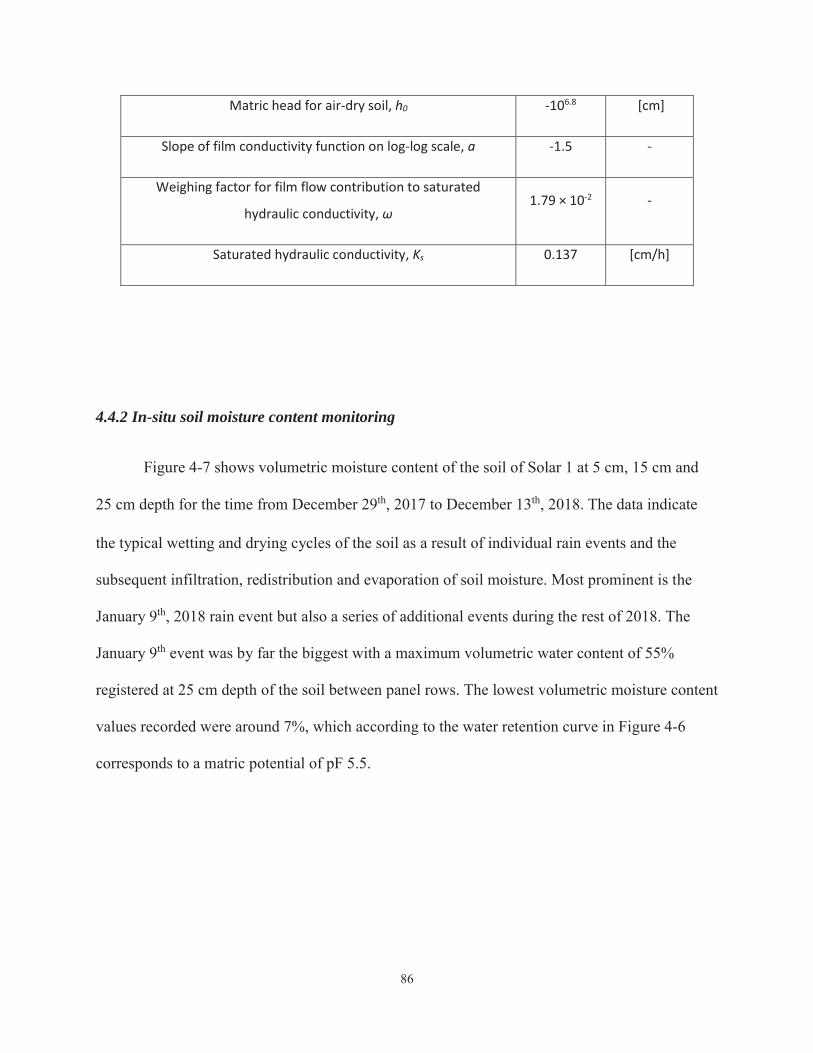
86
Matric head for air-dry soil, h0 -106.8 [cm]
Slope of film conductivity function on log-log scale, a -1.5 -
Weighing factor for film flow contribution to saturated
hydraulic conductivity, ω 1.79 × 10⁻² -
Saturated hydraulic conductivity, Ks 0.137 [cm/h]
4.4.2 In-situ soil moisture content monitoring
Figure 4-7 shows volumetric moisture content of the soil of Solar 1 at 5 cm, 15 cm and
25 cm depth for the time from December 29th, 2017 to December 13th, 2018. The data indicate
the typical wetting and drying cycles of the soil as a result of individual rain events and the
subsequent infiltration, redistribution and evaporation of soil moisture. Most prominent is the
January 9th, 2018 rain event but also a series of additional events during the rest of 2018. The
January 9th event was by far the biggest with a maximum volumetric water content of 55%
registered at 25 cm depth of the soil between panel rows. The lowest volumetric moisture content
values recorded were around 7%, which according to the water retention curve in Figure 4-6
corresponds to a matric potential of pF 5.5.
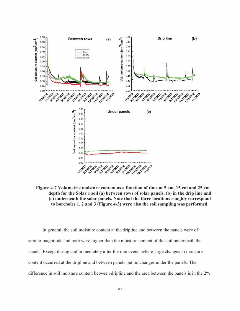
87
Figure 4-7 Volumetric moisture content as a function of time at 5 cm, 15 cm and 25 cm depth for the Solar 1 soil (a) between rows of solar panels, (b) in the drip line and (c) underneath the solar panels. Note that the three locations roughly correspond to boreholes 1, 2 and 3 (Figure 4-3) were also the soil sampling was performed.
In general, the soil moisture content at the dripline and between the panels were of
similar magnitude and both were higher than the moisture content of the soil underneath the
panels. Except during and immediately after the rain events where large changes in moisture
content occurred at the dripline and between panels but no changes under the panels. The
difference in soil moisture content between dripline and the area between the panels is in the 2%

88
to 5% range, which is not as big as expected but potentially big enough to allow faster water
flow in the soil of the driplines compared to soil between the panels. Especially considering the
strong dependency of hydraulic conductivity on water content as shown in Figure 4-6. A more
in-depth analysis of the soil moisture difference between soil of the drip line and between the
solar panels may help to further assess the importance of concentrated infiltration.
The data also shows that after a big event such as the one from January 9th ,2018, soil
moisture content goes back to some “background level” within about one month. This
background level seems to be dependent on the location. I.e. the level is higher under the panels
and the driplines compared to the areas between the panels. Smaller events during spring,
summer and fall 2018 seem not to have a lot of impact on the soil moisture content and were
predominantly recorded in 5 cm but not in 15 cm or 25 cm depth. The only two storm events in
2018 that had an impact on soil moisture content all the way to 25 cm depth were the events
from January 9th and July 9th ,2018. The two events were therefore used for evaluating the soil
moisture simulations using HYDRUS-2D presented in Figures 4-8 to 4-13. The January 9th event
together with an event on March 10th ,2018 was used to further explore the two-dimensional soil
moisture distributions as shown in Figures 4-14 and 4-15.
4.4.3 Soil moisture modeling
This section presents comparisons between measured and simulated volumetric moisture
content of the soil of Solar 1. Figures 4-8 to 4-10 show the results from soil moisture simulations
for the large winter storm that occurred on January 9th ,2018.

89
Figure 4-8 Measured vs. simulated soil moisture content at 5cm, 15cm and 25 cm depth in the soil between the solar arrays. The simulations were run for a winter storm
that lasts from January 1st to March 31th, 2018. Assuming actual evaporation (ET) being equal to 5%, 10% and 20% respectively of potential
evapotranspiration (PET).

90
Figure 4-9 Measured vs. simulated soil moisture content at 5cm and 25 cm depth in the soil at the dripline.

91
Figure 4-10 Measured vs. simulated soil moisture content at 15cm and 25 cm depth in the soil under the solar panel.
Simulations were run for a three-month period from January 1st to March 31th, 2018
assuming actual evaporation (ET) being equal to 5%, 10% and 20%, respectively, of potential
evapotranspiration (PET) according to Equation [2]. Figure 4-8 shows soil moisture content
between the rows of panels, Figure 4-9 shows soil moisture content at the dripline and Figure 4-

92
10 soil moisture content underneath the panels. For the three locations, the HYDRUS-2D model
was able to capture the general soil moisture trend but was unable to simulate all the different
soil moisture features that the TDR probes picked up. Calculated agreed best with measured
values from the soil at the dripline (Figure 4-9) and underneath the panels (Figure 4-10). The
former is quite interesting since the dripline is the area with the highest moisture dynamics. The
latter is less surprising since not much soil moisture change occurs underneath the panel. The
HYDRUS-2D model was not able to simulate well the moisture content of the soil between the
panels (Figure 4-8). A possible reason is that the soil between the panels is more heterogenous
than assumed by the HYDRUS-2D model. I.e. the hard soil layer found in borehole #1 of the soil
between panels may have an effect but that the current HYDRUS-2D model cannot capture. It
was also noticed that during rain events water tend to pond on the soil between panels, which
HYDRUS-2D cannot take into account but may also considerably affect infiltration and water
redistribution of rainwater within the soil between panel. Based on the simulations for the
dripline, n = 10% provided the best agreement between measurements and simulations.
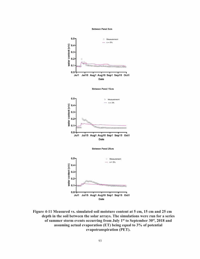
93
Figure 4-11 Measured vs. simulated soil moisture content at 5 cm, 15 cm and 25 cm depth in the soil between the solar arrays. The simulations were run for a series
of summer storm events occurring from July 1st to September 30st, 2018 and assuming actual evaporation (ET) being equal to 3% of potential
evapotranspiration (PET).

94
Figure 4-12 Measured vs. simulated soil moisture content at 5 cm and 25 cm depth in the soil of the dripline.

95
Figure 4-13 Measured vs. simulated soil moisture content at 15cm and 25 cm depth in the soil under the solar panel.
Figures 4-11 to 4-13 show the results from simulations for a series of summer storms that
occurred on July 9th ,2018. Simulations were run for a three-month period from July 1st to
September 30th ,2018 assuming actual evaporation (ET) being equal to 3% of potential
evapotranspiration (PET) according to Equation [2]. Figure 4-11 shows soil moisture content
between the rows of panels, Figure 4-12 shows soil moisture content at the drip line and Figure

96
4-13 soil moisture content underneath the panels. Similar to the results for the winter event
presented in Figures 4-8 to 4-10, HYDRUS-2D was able to capture the general soil moisture
trend but was unable to capture all soil moisture features that the TDR probes picked up. Similar
to the winter storm, calculations agreed best with measurements for the soil at the dripline
(Figure 4-12) and underneath the panels (Figure 4-13). The HYDRUS-2D model, however,
failed to simulate the measured moisture content time series of the soil between the panels
(Figure 4-11). The latter was rather surprising since the measured soil moisture time series
shown in Figures 4-11 are similar to ones found by Dijkema et al. (2018) and Luo et al.
(2019a,b) in their studies on water redistribution in arid soil. Luo et al. (2019a,b) were able to
successfully simulate the soil moisture time series with the same constitutive relationships used
for this study. So, some properties specific to the soil between the solar panel cannot be captured
by the HYDRUS-2D model develop in this study. What these properties are would have to be
explored in a follow up study.

97
Figure 4-14 Moisture redistribution in the Solar 1 soil before, during and after the January 9th ,2018 storm event.

98
Figure 4-15 Moisture redistribution in the Solar 1 soil before, during and after the March 10th ,2018 storm event.

99
Figures 4-14 and 4-15 show the moisture redistribution in the Solar 1 soil before, during
and after storm event on January 9th and March 10th ,2018. For the simulation of the January 9th
event, a homogenous initial soil moisture distribution and volumetric moisture content of 10%
was assumed for the soil profile. For the simulation of the March 10th event, however, the final
moisture content distribution of the simulations for the January 9th event were used as initial
conditions, as shown in the top panel, Day 62, of Figure 4-15. As expected, based on the
conceptual model of concentrated infiltration shown in Figure 4-1, concentrated infiltration does
occur along the four drip lines. Also as expected, infiltration was highest at the drip line of the
lower edged of the panels where rainwater dripping off the panels infiltrates together with
rainwater reaching the ground between the panel rows. However, moisture content levels as well
as infiltration depths in the soil at the driplines were only slightly higher than in the soil between
the solar panels. I.e. although concentrated infiltration does occur, it does not seem to lead to
much deeper infiltration into the soil at the drip lines compared to the soil between the solar
panels. At least if assuming a homogenous initial soil moisture distribution. Preliminary
calculations by Luo et al. (2016, 2017) for Solar 1 showed a more pronounced concentrated
infiltration effect. They did, however, use hydraulic properties of the more-sandy SEPHAS
Lysimeter 1 soil and assumed higher precipitation rates than were used for this study based on
actual measurement for Solar 1 soil and meteorological conditions. Within the first 48 hours after
the January 9th storm (Figure 4-14, Day 5, lowest panel), the infiltration fronts from the four drip
lines remain separated but eventually merge, as the top panel, Day 62, of Figure 4-15 shows. It is
interesting to note that event 60 days after the January 9th event, the moisture distribution (Figure
4-15, Day 62) in the soil is not completely homogenous yet and areas of concentrated infiltration

100
are remaining visible. With the second storm occurring on March 10th,2018, concentrated
infiltration occurs again at the drip lines, which seem to reinforce the concentrated infiltration
patter, although the March 10th,2018 storm was much smaller than the January 9th storm. Figures
4-14 and 4-15 show that the initial, or antecedent, moisture content plays a role in terms of
infiltration pattern. A follow up study that simulates a series of storms events over say a one-year
period could shed light on whether these areas of concentrated infiltration develop into conduits
of deeper infiltration, especially for smaller storm events, and therefore might have a profound
impact on the water balance of a soil under arrays of solar panels. Figures 4-7a and 4-7b shows a
slight but potentially important difference in moisture content between the soil between the
panels and at the drip line.
4.5 CONCLUSIONS
The study shows that in the presence of rows of solar PV panels such as at Solar 1,
rainfall is concentrated along the driplines, which causes deeper infiltration of rainwater along
the driplines compared to areas between rows and no infiltration underneath a row of solar PV
panels. This finding is in accordance with recent lysimeter studies on infiltration into and
evaporation off bare, arid soil (Koonce, 2016; Lehmann et al., 2019) that shown that the deeper
rainwater infiltrates into the soil, the less likely it is to evaporate back into the atmosphere.
HYDRUS-2D calculated agreed best with measured moisture content values from the soil
at the dripline and underneath the panels. The former is quite interesting since the dripline is the
area with the highest moisture dynamics. The latter is less surprising since little soil moisture
change occurs underneath the panel. The HYDRUS-2D model, however, had only limited
success in simulating the moisture content of the soil between the panels. A possible reason is

101
that the soil between the panels is more heterogenous than assumed by the HYDRUS-2D model.
It was also noticed that during rain events water tend to pond on the soil between panels, which
HYDRUS-2D cannot take into account but may considerably affect infiltration and water
redistribution of rainwater within the soil between panel.
HYDRUS-2D simulations also indicated that initial, or antecedent, moisture content
plays a role in terms of infiltration pattern. A follow up study that simulates a series of storms
events over say a one-year period could shed light on whether areas of concentrated infiltration
in the drip line indeed develop into conduits of deeper infiltration, especially for smaller storm
events, and therefore might have a profound impact on the water balance of a soil under arrays of
solar panels. Moisture measurements in the soil of the dripline as well as between the rows of
solar panels shows a small but potentially important difference in moisture content, especially
considering how sensitive soil hydraulic conductivity is on soil moisture content.
4.6 REFERENCES
Dana, G. L., J. R. Batista, M. Berli, R. F. Boehm, and S. M. Dascalu (2012), The Solar Energy Water-Environment Nexus in Nevada, Reno.
Dijkema, J., J. Koonce, R. Shillito, T. Ghezzehei, M. Berli, M. Van der Ploeg and M. T. Van Genuchten (2016). "Simulating water redistribution in an arid soil of a large weighing lysimeter." Vadose Zone Journal: in preparation.
Huang, J (Huang, Jun); Wu, PT (Wu, Pute)[ 4,5 ] ; Zhao, XN (Zhao, Xining) Effects of rainfall intensity, underlying surface and slope gradient on soil infiltration under simulated rainfall experiments
Koonce, J.E. (2016) Water Balance and Moisture Dynamics of an Arid and Semi-Arid Soil: A Weighing Lysimeter and Field Study, University of Nevada Las Vegas, Las Vegas, NV.

102
Lehmann, P., Berli, M., Koonce, J.E. and Or, D. (2019) Surface evaporation in arid regions: Insights from lysimeter decadal record and global application of a surface evaporation capacitor (SEC) model. Geophysical Research Letters 46(16), 9648-9657.
Luo, Y., Koonce, J., Shillito, R., Dijkema, J., Ghezzehei, T.A., Berli, M. and Yu, Z. (2016) The impact of solar arrays on arid soil hydrology: some numerical simulations pp. EOS-Abstract No. H21C-1421, American Geophysical Union, San Francisco, CA.
Luo, Y., Koonce, J.E., Shillito, R.M., Dijkema, J., Ghezzehei, T.A. and Berli, M. (2017) Understanding the impacts of solar arrays on arid soil hydrology, Nevada EPSCoR Office, Las Vegas, NV.
Peters, A., 2013. Simple consistent models for water retention and hydraulic conductivity in the complete moisture range. Water Resources Research 49, 6765–6780. https://doi.org/10.1002/wrcr.20548
Peters, A., 2014. Reply to comment by S. Iden and W. Durner on ‘“Simple consistent models for water retention and hydraulic conductivity in the complete moisture range.”’ Water Resources Research 2781–2786. https://doi.org/10.1002/2012WR013341.Reply
Prinz, D. (1996) Sustainability of Irrigated Agriculture. In: Pereira, L.S. (ed) Sustainability of Irrigated Agriculture, Balkema, Rotterdam. pp. 135-144
Richard G. Allen; Luis S. Pereira; Dirk Raes; Martin Smith (1998). Crop Evapotranspiration – Guidelines for Computing Crop Water Requirements. FAO Irrigation and drainage paper 56. Rome, Italy: Food and Agriculture Organization of the United Nations. ISBN 978-92-5-104219-9.
Richards, L.A. (1931) Capillary conduction of liquids through porous mediums. Physics 1(5), 318-333.
Robinson, David A. (2008), "Field Estimation of Soil Water Content: A Practical Guide to Methods, Instrumentation and Sensor Technology", Soil Science Society of America Journal, Vienna, Austria: International Atomic Energy Agency, 73 (4).
Šimůnek, J., van Genuchten, M.T. and Sejna, M. (2006) The HYDRUS Software Package for Simulating Two- and Three-Dimensional Movement of Water, Heat, and Multiple Solutes in Variably-Saturated Media, Czech Republic.

103
Šimůnek, J., van Genuchten, M.T. and Sejna, M. (2016) Recent developments and applications of the HYDRUS computer software packages. Vadose Zone Journal 15(7).
Sinha, P., Hoffmann, B., Sakers, J. and Lynnedee, A. (2018) Best Practices in Responsible Land Use for Improving Biodiversity at a Utility-Scale Solar Facility. Case Studies in the Environment, 1-12.
Soil Survey Division Staff, (1993) Soil Survey Manual, US Department of Agriculture. 437 p.

104
CHAPTER 5
CONCLUSIONS
Desert soils cover about one third of the Earth’s land surface. Despite their large extent
and critical role for infiltration, redistribution and evapotranspiration of the sparse precipitation
in desert environments, our understanding of desert soil hydraulic processes and properties is still
rather limited. A recent study by Dijkema et al. (2018) introduced a modeling framework to
simulate the moisture dynamics of a bare, desert soil. Their model used bimodal van Genuchten-
Mualem (BVG) hydraulic functions (van Genuchten, 1980) and was able to capture water
redistribution under infiltration as well as evaporation conditions. For the latter, however, only
when the soil was relatively moist (volumetric moisture content >10%, matric head < pF 2). For
dryer soil conditions, however, as they occur between rainfall events and are typical for desert
soils most of the time, the model consistently underestimated evaporative fluxes and,
subsequently, overestimated soil moisture content. Dijkema et al. (2018) hypothesized that the
BVG hydraulic conductivity function (Mualem, 1976; van Genuchten, 1980), may not be ideal
for drier soil conditions since it cannot take film flow into account and an alternative hydraulic
conductivity model might be needed that can capture liquid water flow for drier soil conditions.
Therefore, the overarching goal of my thesis was to explore and test alternative hydraulic
functions that could help us better simulate water infiltration into and evaporation off arid soils
and, eventually, to improve our understanding of the moisture dynamics of near-surface desert
soils.
As described in Chapter 2, I focused first on improving the model by Dijkema et al.
(2018) to capture soil moisture condition dryer than pF 2 or 32% water saturation during

105
evaporation. For that purpose, I replaced the bimodal van Genuchten-Mualem (BVG) water
retention and hydraulic conductivity functions in the model by Dijkema et al. (2018) with the
corresponding functions from the Peters-Durner-Iden (or PDI) model (Peters, 2013, 2014), which
can capture the capillary as well as film flow of liquid water in the soil. I also measured water
retention and hydraulic conductivity functions of the Lysimeter 1 soil, the same soil used by
Dijkema et al. (2018), employing a combination of evaporation and absorption tests with
HYPROP and WP4-C devices. I found that the PDI water retention functions (Peters, 2014)
better represent the measured water retention curves than the BVG water retention functions
used by Dijkema et al. (2018). In particular for the critical range of volumetric moisture contents
between 5% and 10% (saturation degrees between 16% and 32%, and matric heads between pF 2
and 4). The BVG water retention functions predicted higher suctions (lower matric heads) than
the PDI functions for volumetric moisture contents in the range from 5 to 10%, likely leading to
an underestimation of the hydraulic conductivity values and subsequently water fluxes in the soil
in the range from 5% to 10%. Interestingly, the BVG and PDI hydraulic conductivity functions
were not noticeably different within the range between pF 2 and 3 where most of the HYPROP
measurements were available. For pF values higher than 3, however, the PDI functions predicted
higher hydraulic conductivity values than the BVG functions. Therefore, the hypothesis put
forward by Dijkema et al. (2018) that including film flow may improve model predictions could
be confirmed for pF > 3. For pF values between 2 and 3, however, is probably rather the
difference between BVG and PDI water retention than hydraulic conductivity functions that led
to the improved soil moisture simulations. A comparison between BVG-based and PDI-based
simulations for the same soil moisture calibration and validation datasets already used by
Dijkema et al. (2018) showed that the model by Dijkema et al. (2018) using PDI instead of BVG

106
hydraulic functions (hereafter called the Luo et al. (2019a) model) provided better soil moisture
content predictions, especially for soil moisture levels less than 10% (lower than 32% saturation,
higher than pF 2). In other words, replacing the BVG water retention and hydraulic conductivity
functions in the model by Dijkema et al. (2018) with the corresponding functions from the PDI
model (Peters 2014) considerably improved the ability of the model by Dijkema et al. (2018) to
capture soil moisture condition dryer than pF 2 or 32% water saturation.
In a second step (Chapter 3), I tested the Luo et al. (2019a) model on a soil moisture
dataset from the top 50 mm of the Lysimeter 1 soil, which provided lower moisture content
values at higher spatial resolution than the datasets used by Dijkema et al. (2018). The dataset
showed that only the top 20 mm of the Lysimeter 1 soil profile dry out completely (i.e. reach a
soil moisture content below the detection limit of the soil moisture sensors) over the five months
period whereas the soil moisture contents between 20 to 50 mm depths converge towards some
equilibrium moisture contents ranging between 3.5% and 5% (or 15% to 21% saturation,
respectively). I compared measured soil moisture time series for different depth with simulations
using the model by Luo et al. (2019a) and found that the latter is able to quite accurately forward
simulate soil moisture redistribution in the top 50 mm of the soil profile for a wide range of soil
moisture contents from 15% to over 90% saturation using only independently determined soil
physical parameters as well as precipitation and evaporation as flux boundary conditions.
Measurements and simulations show that soil moisture from the top 50 mm evaporates back into
the atmosphere within one month or less after a rain event. The spatial and temporal soil
moisture distribution of the top 50 mm during evaporation point toward a two-step evaporation
process as proposed by Shokri et al. (2009) and Or et al. (2013), which could not be fully
captured by Luo et al. (2019b).

107
In a third and final step, (Chapter 4) I applied the model by Luo et al. (2019a) to simulate
the impact of an array of photovoltaic (PV) solar panels on the water distribution in the soil
underneath and between rows of PV solar panels as a function of precipitation and evaporation
using HYDRUS-2D (Šimůnek et al., 2006, 2016). The goal here was to assess the impact of solar
arrays on the precipitation reaching the soil surface and this change in spatial precipitation
pattern on the moisture distribution within the soil profile underneath a PV solar facility. I was
particularly interested in how solar arrays may lead to concentrated infiltration of rainwater into
the soil and whether this change of infiltration pattern has an impact on the water balance of the
soil within the solar facility. The HYDRUS-2D simulations showed that the solar PV panels
caused concentrate rainfall along the drip lines of the panels, which led to deeper infiltration of
rainwater into the soil along the drip lines compared to areas between solar panel rows and, as
expected, no infiltration underneath a row of solar PV panels. HYDRUS-2D calculations agreed
best with measured moisture content values from the soil at the drip line and underneath the
panels. The former is quite interesting since the drip line is the area with the highest moisture
dynamics. The HYDRUS-2D model, however, had only limited success in simulating the
moisture content of the soil between the panels. A possible reason is that the soil between the
panels is more heterogenous than assumed by the HYDRUS-2D model. It was also noticed that
during rain events water tend to pond on the soil between panels, which HYDRUS-2D cannot
take into account but may have a considerably impact on water infiltration and water
redistribution of rainwater within the soil between panel.
As next steps, I would further explore whether the PDI model could capture water
redistribution at volumetric soil moisture contents even lower than 3.5% (pF >4.7), maybe as low
as 2%, which would correspond to air-dry conditions for Lysimeter 1 soil, assuming an average

108
air relative humidity of 60% (at 25˚C). The PDI model (Peters, 2013) includes a vapor flow
component, which has not been considered for this study but could be employed to simulate
water flow at even lower moisture content. In terms of water redistribution due to PV solar
panels, it would be worth to run additional simulations on a series of storms events over say a
one-year period that could shed light on whether areas of concentrated infiltration in the soil
below the dripline can be sustained and develop into permanent conduits for deeper infiltration.
Especially for moisture from smaller storm events that might otherwise get caught in and
evaporate off the dry soil near the surface. Such preferential flow paths, if sustainable, might
have a profound impact on the water balance of a soil under arrays of solar panels. Moisture
measurements in the soil of the dripline as well as between the rows of solar panels shows a
small but potentially important difference in moisture content, especially considering how
sensitive soil hydraulic conductivity is on soil moisture content. Last but not least, I would like to
take advantage of the insight I gained by compiling my thesis and develop an antecedent
moisture content model for desert environments based simplified infiltration, redistribution and
evaporation calculations. Maybe similar to the SEC model developed by Or and Lehmann (2019)
and tested on the SEPHAS lysimeter soils by Lehmann et al. (2019).
The work presented in this thesis has shown how the soil moisture distribution in the top
100 mm of a bare desert soil changes as a function of precipitation and evaporation. It also
confirms that the model by Luo et al. (2019) is able to simulate the moisture dynamics of a bare,
near-surface desert soil from near-saturation to about twice the air-dry moisture content. It has
also shown how the soil moisture distribution in the top 50 mm of a bare desert soil changes as a
function of precipitation and evaporation for several months without precipitation. The
HYDRUS-2D simulations in combination with measurements shed light on how rows of PV

109
solar panels affect the soil moisture distribution between and underneath the panels and how
initial, or antecedent, moisture content may play a role in terms of infiltration pattern. Overall, I
think, this thesis contributes to improve our understanding and ability to simulate the moisture
dynamic of bare, near-surface desert soils and will be hopefully helpful to guide human activities
in the desert, such as urban development, recreation and renewable energy generation, while
minimizing their impact on fragile desert environments world-wide.

110
APPENDIX A. : SOIL SAMPLING AT THE DRI “SOLAR 1” PV
FACILITY IN LAS VEGAS
Soil samples were collected between the panels (borehole #1), in the drip line (borehole
#2) a and underneath the panels (borehole #3) of the DRI Solar 1 facility. An initial test drill
showed pretty soft soil from 0-4”, overlying a harder layer between 4” and 10” that (looks like a
thin petrocalcic horizon, Figure 4-4) overlying a much softer layer between 10 and 14”.
Sampling depth was limited by the length of the drill bit. Soil was loosened by drilling to specific
depths of 4”, 10” and 14” using a power drill (Figure A-1). The loose soil was collected from the
borehole with a vacuum cleaner and sampled in individual Ziploc bags (Figure A-2 and A-3). A
minimum of 500 g of soil was collected from 0-4”, 4”-10” and 10”-14” depths. In terms of
hydrologic properties, the petrocalcic horizon from 4”-10” depth is likely going to influence
water infiltration, redistribution and evaporation. Gravimetric moisture content of the samples
will be determined in our soil lab. The hope is that these gravimetric moisture content data can
be correlated with corresponding volumetric moisture content readings from 5, 15 and 25 cm
depth for 12/20/2018. This would then allow to estimate bulk density for the three depth.

111
Figure A-1 Ryan operating the power drill at borehole #2

112
Figure A-2 Yuan vacuuming out borehole #1 between the panels
Figure A-3 Yuan, Ryan and Brian sampling soil from 0-14” depth at borehole #2

113
APPENDIX B. : VAN GENUCHTEN FOR SOILS OF VARIOUS
SOLAR INSTALLATIONS IN NEVADA
During our simulations, we found that the values of different soil types have a
significant impact on the water infiltration depth in soil, thus a study about varying values is
done based on the real soil types in Nevada’s solar facilities.
There are several solar power plants around Las Vegas and in the Mojave Desert
supporting power to the electricity grid. By using the Web Soil Survey (WSS) from USDA,
which provides soil data and information produced by the National Cooperative Soil Survey, we
accessed to the soil information on each solar power plant’s site. Table B-1 shows the soil
information of all the solar power plant.
Table B-1 values of some solar power plants in Nevada
Projects Location Soil Types Alpha range(based
on UNSODA) Alpha range(based on
Soil Survey) 1 Apex Nevada
Solar 36.392690, -114.964868
H1 - 0 to 3 inches: very gravelly loam; H2 - 3 to 15 inches:
extremely gravelly sandy loam; H3 - 15 to 42 inches: cemented
material; H4 - 42 to 60 inches: extremely gravelly sandy loam
0.021 0.075
2 Crescent Dunes
38.241154, -117.363707
H1 - 0 to 8 inches: loamy fine sand; H2 - 8 to 60 inches: loamy fine
sand
0.035 0.124
3 Las Vegas Valley Water
District (Spring
Mountain - Durango
Reservoir and Pumping Station)
36.125105, -115.285973
H1 - 0 to 1 inches: gravelly loamy fine sand; H2 - 1 to 18 inches: loamy fine sand; H3 - 18 to 60
inches: stratified extremely gravelly sand to very gravelly
loamy fine sand
0.035 0.124-0.145
4 Mountain View Solar
near Apex.NV H1 - 0 to 3 inches: very gravelly loam; H2 - 3 to 15 inches:
extremely gravelly sandy loam; H3 - 15 to 42 inches: cemented
material; H4 - 42 to 60 inches: extremely gravelly sandy loam
0.021-0.025 0.036-0.075

114
5 Nellis Air Force Base Solar Star
36.257716, -115.055129
H1 - 0 to 1 inches: gravelly fine sandy loam; H2 - 1 to 7 inches: fine
sandy loam; H3 - 7 to 11 inches: gravelly sandy clay loam; H4 - 11
to 15 inches: indurated
0.021-0.033 0.059-0.075
6 Nellis Solar Array II
near Nellis Solar Star
H1 - 0 to 1 inches: gravelly fine sandy loam; H2 - 1 to 7 inches: fine
sandy loam; H3 - 7 to 11 inches: gravelly sandy clay loam; H4 - 11
to 15 inches: indurated
0.021-0.033 0.059-0.075
7 Nevada Solar One
35.801421, -114.982052
H1 - 0 to 1 inches: extremely gravelly sandy loam; H2 - 1 to 9
inches: very gravelly sandy loam; H3 - 9 to 60 inches: extremely
gravelly sand
0.021-0.035 0.075-0.145
8 Searchlight Solar
35.485838, -114.934132
H1 - 0 to 2 inches: very gravelly sandy loam; H2 - 2 to 6 inches:
very gravelly sandy clay loam; H3 - 6 to 16 inches: bedrock
0.021-0.033 0.059-0.075
9 Silver State Solar North
35.622797, -115.350674
H1 - 0 to 1 inches: extremely gravelly sandy loam; H2 - 1 to 9
inches: very gravelly sandy loam; H3 - 9 to 60 inches: extremely
gravelly sand
0.021-0.035 0.075-0.145
10 Spectrum Nevada Solar
36.232988, -114.881701
H1 - 0 to 2 inches: gypsiferous sandy loam; H2 - 2 to 4 inches:
gypsiferous material; H3 - 4 to 19 inches: gypsiferous material; H4 -
19 to 29 inches: gypsiferous bedrock
0.021 0.075
So based on Table B-1, the range of the soil where the solar facilities built upon are
0.021-0.035 ( UNSODA) and 0.036-0.145 (Soil Survey).
115
CURRICULUM VITAE
Yuan Luo
E-mail: [email protected]
EDUCATION
Ph.D. candidate, Geoscience, University of Nevada, Las Vegas, 2017
Concentrations: Hydrogeology
Dissertation: Moisture Dynamics of a Near-surface Desert Soil
M.S., Civil Engineering, University of Kansas, 2013
Concentrations: Water Resources Engineering
Thesis: Estimating the Ordinary High Water Discharge for Kansas Streams.
B.S., Civil Engineering, North China University of Water Resources and Electric Power, 2011
Concentrations: Water Resources and Hydropower Engineering
Project: The Designing of Concrete Dam in Chushuidong Reservoir in Pan County
WORK EXPERIENCES
Graduate Research Assistant, University of Nevada, Las Vegas, 2014 – 2019
Graduate Research Assistant, University of Kansas, 2012 – 2013
Technician, Yellow River Construction Company, 2011 – 2012
CONFERENCES ATTENDED
American Geophysical Union (AGU) Fall Meeting – 2016, 2017
Solar Energy-Water-Environment Nexus in Nevada Annual Meeting – 2015, 2016, 2017

116
Nevada Water Resources Association Annual Conference – 2015
PRESENTATIONS
Luo, Y., Koonce, J., Dijkema, J., Shillito, R., Ghezzehei, T., & Berli, M. (2018, April). Modeling Water Redistribution in a Near-Surface Desert Soil. Poster session presented at the annual meeting of EGU, Vienna, Austria.
Luo, Y., Koonce, J., Dijkema, J., Ghezzehei, T., & Berli, M. (2017, December). Modeling Water Redistribution in a Near-Surface Arid Soil. Poster session presented at the annual meeting of AGU, New Orleans, LA.
Luo, Y., Koonce, J., Dijkema, J., Shillito, R., Ghezzehei, T., & Berli, M. (2016, December). The Impact of Solar Arrays on Arid Soil Hydrology: Some Numerical Simulations. Poster session presented at the annual meeting of AGU, San Francisco, CA.