Module 6odu e 6Image Denoising and Nonlinear

• Noise ModelsFiltering

• Morphological and Order Statistic Filters

• Bilateral Filter• Bilateral Filter

• Anisotropic Diffusion

• Non-local (NL) Means

• Wavelet Soft Thresholdingg

• BM3D

• Homomorphic Filtering• Homomorphic Filtering1

IMAGE NOISE MODELS• To proceed further in understanding and designing non-linear

filters, we will need to deepen our statistical modeling of noise.

• Any channel (electrical wire, airwaves, optical fiber) is imperfect. Images sent over a channel always suffer a degradation of information:

(a) static (high-frequency noise or thermal noise)(b) bit errors(b) bit errors(c) sensor noise

• These errors degrade- visual interpretation

2- computer image analysis

White Noise is Uncorrelated Noise

• Assume the additive white noise model:

J = I + N

where I is an original image and N a digital white noise image.where I is an original image and N a digital white noise image.

• White noise suggests an (on average) a flat spectrum.

• An equivalent meaning is that the elements N(m, n) of N are uncorrelated: any two elements N(m, n), N(p, q) of the noise matrix N (where (m, n) ≠ (p, q)) affect one another little or not at all.( ( , ) ≠ (p, q))

• Mathematically this is equivalent to the noise being white.

3

R f N iRange of Noise

• The set of values ℜN the noise can take. In digital images the noise must be discrete integers. However,

ill i t ti d lwe will use approximate continuous models.

• For additive noise the noise range is usually symmetric: ℜN = [-Q, Q] where possibly Q = ∞.

• For multiplicative noise assume the noise range is non-negative: ℜN = [0, Q] where possibly Q = ∞.

4

Probability Density Function ofProbability Density Function of Noise

• The probability density function or PDF fN(q) is a modelof the probabilities of N(m n):of the probabilities of N(m, n):

Pr{a < N(m n) < b} =bf (q)dq NPr{a < N(m, n) < b}

where [a b] ⊆ ℜN

af (q)dq N

where [a, b] ⊆ ℜN.

• Assume that all elements N(m n) of N obey theAssume that all elements N(m, n) of N obey the identical probability model - the same PDF.

5• So, fN(q) is not expressed as a function of (m, n).

Properties of PDF

• Two basic properties of the PDF

(1) fN(q) ≥ 0 for all q ∈ ℜN

(2) = 1f (q)dq NNℜ

• Note: (1) and (2) imply that fN(q) ≤ 1 for all q ∈ ℜN.

• For symmetric noise: ℜN = [-Q, Q] assume that fN(q) is a symmetric functionN(q) y

fN(q) = fN(-q) 6

G i PDFGaussian PDF

• Here ℜN = [-∞, ∞] and2-(q/σ)1f (q) = eN

with scale parameter σ.

f (q) e2 σπN p (q)

N

• The parameter σ2 is the variance of the PDFTh i h• The most common noise that occurs in applications … and in nature.

• The usual noise found in electrical circuits, most

i i h l

q0

7communication channels, etc.

Laplacian PDFLaplacian PDF• Here ℜN = [-∞, ∞] andN [ , ]

- 2 q /σ1f (q) = e2σN

p (q)N

with scale parameter σ.• Parameter σ2 is again the

2σ

Parameter σ is again the variance.

• Often models impulse noise.p

• Large number of small-amplitude values, and a q0

(relatively) large number of high-amplitude values.

8

Gaussian vs. Laplacian PDFs

GaussianL l iLaplacian

• Laplacian noise is impulsive – a heavy-tailed PDF.9

Laplacian noise is impulsive a heavy tailed PDF.

Exponential PDFExponential PDF• Here ℜN = [0, ∞] andHere ℜN [0, ] and

-q/σ1f (q) = eσN

p (q)N

with scale parameter σ.• Parameter σ2 is again equal to theParameter σ is again equal to the

variance and s is the mean.

• Often models multiplicative• Often models multiplicativenoise.

• A coherent image noise model q0A coherent image noise model (radar, laser, electron microscopy, etc)

10

Salt-and-Pepper (S&P) Noise

• A model for significant bit errors.

• When transmitting digital image data, significant bit errors can occur:

'1' → '0' ('light' → 'dark')'0' → '1' ('dark' → 'light')

• May be due to thermal effects or even gamma rays.

• Salt and pepper noise is not additive.

11

S&P Noise Model

• Let Imax and Imin be the brightest and darkest allowable gray levels in image I (e g 0 & 255)levels in image I (e.g. 0 & 255)

• Define the simple probabilitiess p

(1-p)/2 ; q = -1p (q) = p ; q = 0

If J i th i i th

s-pp (q) p ; q(1-p)/2 ; q = 1

I 1• If J is the noisy image, then minI ; q = -1J(i, j) = I(i, j) ; q = 0

I 1

• This is a simple model for the worst case type of bit errors. maxI ; q = 1

12

Statistical Mean

• The statistical mean of N is

μ q f (q)dq= ⋅N

N Nℜ• It measures the center about which the noise

realizations cluster.realizations cluster.

• For a symmetric PMF (Q can be ∞), Q-Q

μ q f (q)dq =0 ( )= ⋅N N why?

13

Statistical Variance

• The variance of N is

( )22σ q-μ f (q)dq= ⋅N N Nℜ

• The standard deviation σ is the average distance

( )N

N N Nℜ

• The standard deviation σN is the average distancefrom μN that the noise realizations fall.F t i ( ) i th i i• For symmetric (zero-mean) noise, the variance is just 2 2σ q f (q)dq= ⋅N Nℜ

14

σ q f (q)dq= N

N Nℜ

Mean & Variance of PDFs

• Exercises: Show that for Gaussian, Laplacian, and i l PDF h i i 2exponential PDFs, the variance is σ2.

• Also show that for exponential PDF, the mean is equal to σ.q

15

Denoising

• Consider denoising of an image contaminated by white inoise:

image iimagetransmitter

noisy channel imagereceiver

• Two goals of filtering:

S thi d i (bit h l- Smoothing - reduce noise (bit errors, channel, etc)

16- Preservation - of features: edges and detail

S thi P tiSmoothing vs. Preservation

• Image denoising contains conflicting goals:- Smoothing: high noise frequencies are g g q

attenuated- Broadband images: both low and high frequencies are important

• Linear filtering cannot differentiate between desirablehigh frequencies and undesirable high frequencies

• A linear low-pass denoising filter will always:R d hi h f i

17- Reduce high frequency noise- Blur the image

WHY NONLINEAR FILTERING ?

• Linear filtering has important limitations.

• The basis of linear filtering is frequency or g q yspectrum shaping:

reduce (attenuate) unwanted frequencies-reduce (attenuate) unwanted frequencies

- amplify or preserve desired frequencies

18

Motivation for Nonlinear FilteringMotivation for Nonlinear Filtering(or nonlinear processing of linear filter responses)( p g p )

• Generally, nonlinear filtering cannot be expressed by li l i b f h ilinear convolution nor by frequency shaping.

• Some approaches nonlinearly modify linear responses

• Others combine filter bank responses nonlinearly

• We will study these in the important context of imageWe will study these in the important context of imagedenoising.

• The common theme: nonlinear filters give you• The common theme: nonlinear filters give you capabilities that linear filters don't have.

19

MORPHOLOGICAL FILTERSMORPHOLOGICAL FILTERS

20

MORPHOLOGICAL FILTERSMORPHOLOGICAL FILTERS• Recall: For image I, window B, the windowed set at (m,n)

is:BI(m n) = {I(m p n q); (p q) ∈ B}BI(m,n) = {I(m-p, n-q); (p, q) ∈ B} .

• A nonlinear filter F on a windowed set is a nonlinear function of the pixels covered by the window.p y

• Denote the nonlinear filter F on BI(m,n) byJ(m,n) = F{BI(m,n)} = F{I(m-p, n-q); (p, q) ∈ B}

• Performing this at every pixel gives a filtered image:J = F[I, B] = [J(m,n); 0 ≤ m ≤ M-1, 0 ≤ n ≤ N-1]

21

Boundary-of-Image Processing

• As with binary morphological filters: when a i d l " "window overlaps "empty space" …

• Pixel replication is assumed: fill the "empty"

22window slots by the nearest image pixel.

MEDIAN FILTER

• The median filter is a nonlinear filtering device that is related to the binary majority filter (Module 2)to the binary majority filter (Module 2).

• Despite being “automatic” (no design), it is very effective for p g ( g ), yimage denoising.

• Despite its simplicity, it has an interesting theory that justifies its use.

• The median filter is a special member of several classes of filters, including two studied here: gray-level morphologicalfilters, including two studied here: gray level morphological filters, and order statistic filters.

23

Order Statistics

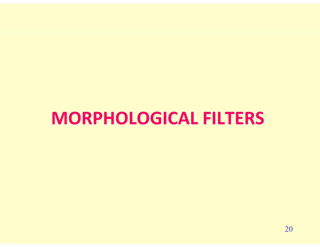
• Definition: Given a set of numbers

{ }1 2 2P+1X = X ,X ,...,X

the order statistics (or OS) of the set are the same elements reordered from smallest to largest.elements reordered from smallest to largest.

• The OS of X are denoted

{ }such that

{ }(1) (2) (2P+1)X = X ,X ,...,X

24(1) (2) (2P+1)X X X≤ ≤ ≤

Special Order Statistics

• In particular:

{ } ( )

{ }1 2 2P+1 1MIN X ,X ,...,X X

MAX X X X X

=

{ } ( )

{ } ( )

1 2 2P+1 2P+1

1 2 2P+1 P+1

MAX X ,X ,...,X X

MED X ,X ,...,X X

=

= ( )

• The median MED is the middle value in rank.

25

Median Filter

• Given image I and window B, the median filtered image is:

J = MED[I B]J MED[I, B]

• Each output is the median of the windowed set:J(m n) = MED{BI(m n)}J(m,n) MED{B I(m,n)}

= MED{I(m-p, n-q); (p, q) ∈ B}

26

Properties of the Median Filter

• The median filter smooths additive white noise.

Th di filt does not de rade ed es• The median filter does not degrade edges.

• The median filter is particularly effective for removing large amplitude noise impulsesremoving large-amplitude noise impulses.

27

Example - 1-D Median Filter

10 10 10

2

6

2

6

2

6

2520151050-2

2520151050-2

2520151050-2

2

image scan line AVE[I, B], B = ROW(3)

• Both filters smooth, but AVE blurs the structures.

MED[I, B], B = ROW(3)

,• Using MED, the "noise" is smoothed effectively - large

noise spikes are eradicated, rather than blurrrrrrrrred.• MED maintains signal structure better the edges are

28

• MED maintains signal structure better - the edges are sharp.

Comments on Window Shape • B = SQUARE smooths noise strongly, but may damage

image details of interest.

• B = CROSS reduces these effects, if known that the image contains horizontal/vertical features.Example: Images of dot-matrix characters.

• If the image contains curvilinear details that are diagonally oriented, then B = CROSS can perform

lpoorly.

• Variations: combine the outputs of multiple CROSS, X-SHAPED ROW COL d b k hSHAPED, ROW, COL, etc. windows e.g. by taking their MED, AVE, etc. These "detail-preserving filters" work pretty well but the theory is heuristic.

29

Erosion and Dilation

• Given an image I and a window B:

J = DILATE[I, B]ifif

J(i, j) = MAX{BI(i, j)} (local max)andand

J = ERODE[I, B]ifif

J(i, j) = MIN{BI(i, j)} (local min)

30

Qualitative Properties ofQualitative Properties of Morphological Filtersp g

l l h l l f l ff h h h h

Ansel Adams’ Joshua Tree

• Gray-level morphological filters effect shape – in this case, the shape of the intensity surface of the image.

• The DILATE (ERODE) filters have the following properties:h f k ( ll )

31- Increase the size of peaks (valleys)- Decrease the size of, or eliminate, valleys (peaks)

Dilation and Erosion Examples

6

10

6

10

2 2

2520151050-2

10DILATE[I, B], B = ROW(3)

2520151050-2

ERODE[I, B], B = ROW(3)10

6

10

6

10

2

2 2

2520151050-2

DILATE[DILATE[I, B], B], B = ROW(3)

2520151050-2

ERODE[ERODE[I, B], B], B = ROW(3)

32Most valleys gone after one pass. All valleys and negative-going impulses gone after two.

Most positive impulses reduced or gone after one pass. After two, all gone.

CLOSE and OPEN Filters

• The CLOSE and OPEN filters are defined by:

J = CLOSE[I, B][ , ]= ERODE [DILATE [I, B], B]

andand

J = OPEN[I, B]= DILATE [ERODE [I, B], B]

33

Properties of CLOSE and OPEN

• Effective smoothing filters similar to the median filter.

• The CLOSE (OPEN) filter has the following ( ) gproperties:

- smooths noisesmooths noise

- preserves edges

di t ti ( iti ) i i l- eradicates negative- (positive-) going impulses

- leaves the signal at approximately the same level

34

Close and Open Examples

10 10

2

6

2

6

2520151050-2

2

2520151050-2

2

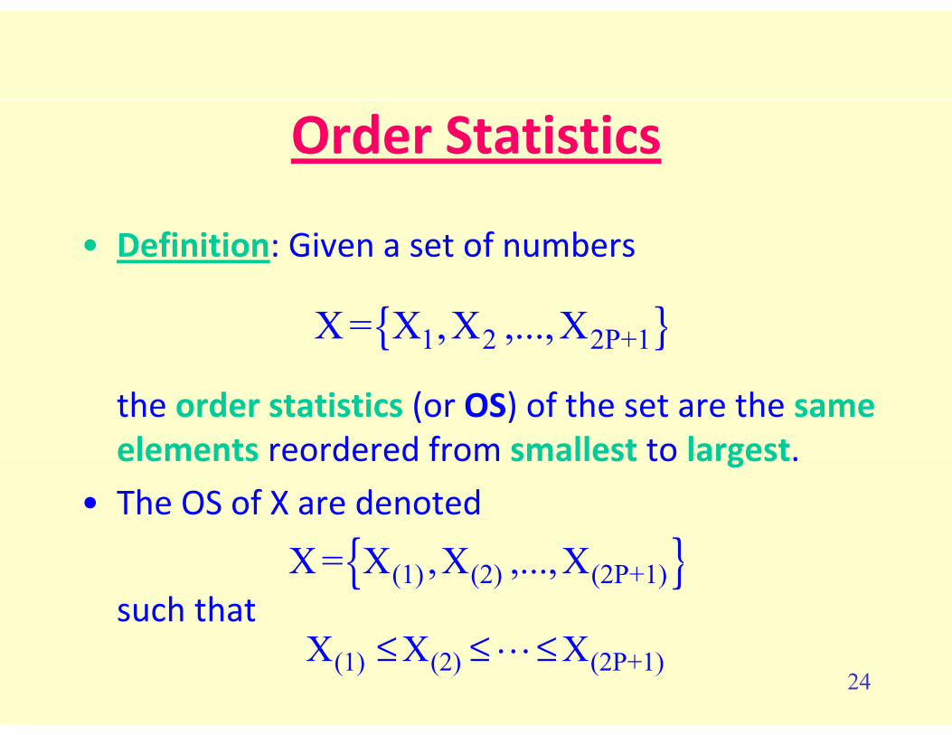
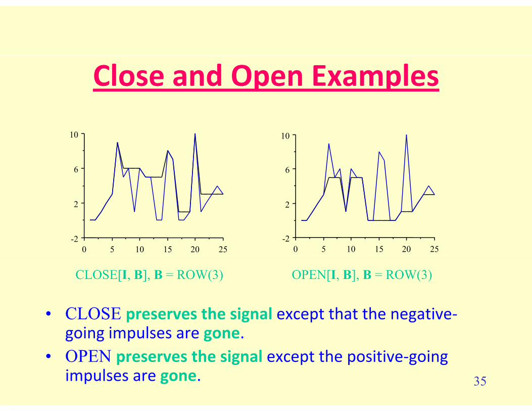
CLOSE[I, B], B = ROW(3) OPEN[I, B], B = ROW(3)

• CLOSE preserves the signal except that the negative-going impulses are gone.

• OPEN preserves the signal except the positive going35

• OPEN preserves the signal except the positive-going impulses are gone.

OPEN-CLOSE & CLOSE-OPEN Filters

• The OPEN-CLOSE and CLOSE-OPEN filters:

J = OPEN-CLOSE [I, B][ , ]= OPEN [CLOSE [I, B], B]

andand

J = CLOSE-OPEN [I, B]= CLOSE [OPEN [I, B], B]

36

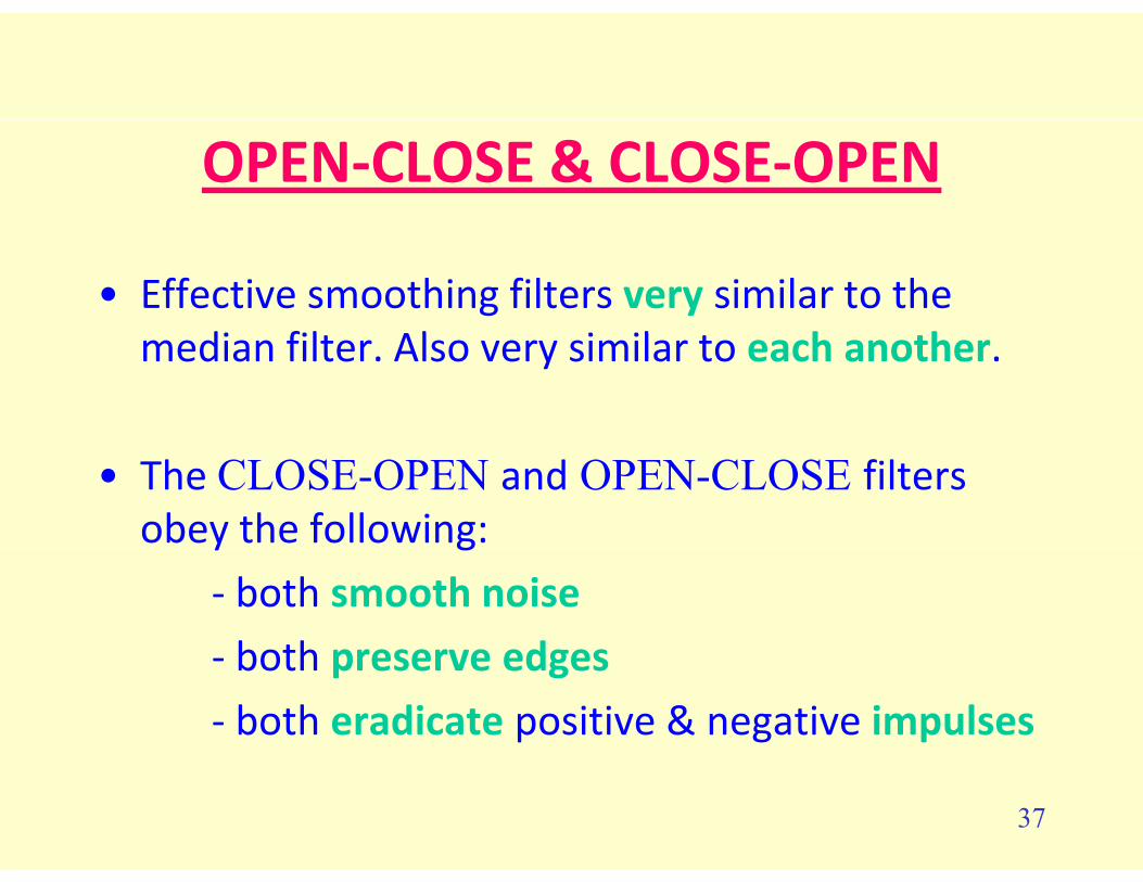
OPEN-CLOSE & CLOSE-OPEN

• Effective smoothing filters very similar to the di fil Al i il h hmedian filter. Also very similar to each another.

• The CLOSE-OPEN and OPEN-CLOSE filtersobey the following:y g

- both smooth noise

both preserve edges- both preserve edges

- both eradicate positive & negative impulses

37

Close-Open & Open-Close Examples

10 10

2

6

2

6

2520151050-2

2

2520151050-2

2

• Note the intense smoothing of noise (especially impulses)

OPEN-CLOSE[I, B], B = ROW(3) CLOSE-OPEN[I, B], B = ROW(3)

g ( p y p )and the retention of the global image structure.

• Note the different possible interpretations of "correct i " d CLOSE OPEN d OPEN CLOSE

38image structure" under CLOSE-OPEN and OPEN-CLOSE.

Application: Peak/Valley Detection

• Suppose we wish to find bright targets or d k tdark spots.

• Difference the OPENed and CLOSEdimage I:

J k = I - OPEN[I, B]Jpeak I OPEN[I, B]Jvalley = CLOSE[I, B] - I

A 'd h i hi hli h• As we'd expect, these operations highlight the peaks and valleys that occur.

39

Peak/Valley Detection Examples

10 10

2

6

2

6

2520151050-2

2

2520151050-2

2

Si l th h ldi (bi i ti ) f th ld

2520151050 2520151050

I-OPEN[I, B], B = ROW(3) CLOS[I, B]-I, B = ROW(3)

• Simple thresholding (binarization) of these could be used to determine the peak and valley locations

40

locations.

Morphological Interpretation

• DILATE and ERODE are true morphological filters in h di d i M d l 2the sense discussed in Module 2.

• As are CLOSE, OPEN, CLOSE-OPEN, and OPEN-CLOSE.

• They have the identical interpretation if we regardy p g

- I as a 3-D binary image with value '1' below its

"plot" and '0' above its "plot"plot and 0 above its plot

- B as a floating 2-D structuring element

41

structuringelement

B

imagefunction

I

Simulated image surface Real image surface

• Leads to fast all-Boolean algorithms &

g g

42

garchitectures.

Morphological Interpretation

ERODE:• When B lies above I, the AND of all it touches is '0'.When B lies above I, the AND of all it touches is 0 .• When B lies below I, the AND of all it touches is '1'.• Whenever B crosses the boundary of I, the AND of all it

t h i '0'touches is '0'.

DILATE:DILATE:• When B lies above I, the OR of all it touches is '0'.• When B lies below I, the OR of all it touches is '1'.• Whenever B crosses the boundary of I, the OR of all it

touches is '1'.

43

Relating Grayscale & BinaryRelating Grayscale & Binary Morphological Filters

• For many morphological filters, there is a precise relationship between the grayscale and binary versions.

• As usual, we will consider the 1D case to develop an understanding of this.

• Here the term m ary is a synonym for grayscale• Here, the term m-ary is a synonym for grayscale.– Implies pixels/samples take one of m distinct values.– For B-bit pixels/samples, m = 2B (= K in Modules 1-3).p / p , ( )

• Several concepts involved:– Threshold decomposition and reconstruction.– The stacking property.– The notion of a positive boolean function or PBF.

44

Threshold DecompositionThreshold Decomposition

• Let x[n] be an m-ary signal• Let x[n] be an m-ary signal.• Define the binary threshold signal

1, [ ] ,[ ]

0 [ ]n x n

x nττ

≥

≥=

for all s.t.

f ll t

• The threshold decomposition of x[n] is

0, [ ] .n x nτ τ≥ < for all s.t.

The threshold decomposition of x[n] is defined by the set of threshold signals x≥τ [n] for τ = [0, 1, 2, …, m-1].for τ [0, 1, 2, …, m 1].

45

Threshold Decomposition ExampleThreshold Decomposition Example

[ ] 5 2 7 0 3 4 • Let B=3, so that m = 2B = 8.

Th i l / l7

[ ] 5 2 7 0 3 4[ ] 0 0 1 0 0 0

x nx n≥

==

• The pixels/samples take values in [0, 7].

• Each threshold signal

6

5

[ ] 0 0 1 0 0 0[ ] 1 0 1 0 0 0

x nx n

≥

≥

== • Each threshold signal

is binary.• In each column, notice

5

4

[ ] 1 0 1 0 0 0[ ] 1 0 1 0 0 1[ ] 1 0 1 0 1 1

x nx n

≥

≥ =

that there must be a stack of 0’s on top of a stack of 1’s

3

2

[ ] 1 0 1 0 1 1[ ] 1 1 1 0 1 1

x nx n

≥

≥

==

a stack of 1 s.• This is called the

stacking property.1

0

[ ] 1 1 1 0 1 1[ ] 1 1 1 1 1 1

x nx n

≥

≥

==

46

0[ ]≥

Threshold ReconstructionThreshold Reconstruction

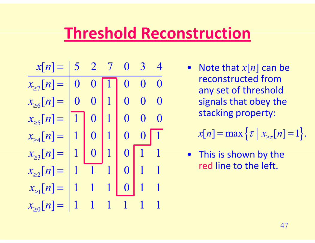
[ ] 5 2 7 0 3 4 • Note that x[n] can be reconstructed from any set of threshold7

[ ] 5 2 7 0 3 4[ ] 0 0 1 0 0 0

x nx n≥

== any set of threshold

signals that obey the stacking property:

6

5

[ ] 0 0 1 0 0 0[ ] 1 0 1 0 0 0

x nx n

≥

≥

==

Thi i h b h

5

4

[ ] 1 0 1 0 0 0[ ] 1 0 1 0 0 1[ ] 1 0 1 0 1 1

x nx n

≥

≥ = { }[ ] max [ ] 1 .x n x nττ ≥= =

• This is shown by the red line to the left.

3

2

[ ] 1 0 1 0 1 1[ ] 1 1 1 0 1 1

x nx n

≥

≥

==

1

0

[ ] 1 1 1 0 1 1[ ] 1 1 1 1 1 1

x nx n

≥

≥

==

47

0[ ]≥

Median Filtering by Threshold g yDecomposition

• On the next page, we will apply a grayscale3-point median filter to x[n]3 point median filter to x[n].

• In parallel, we will apply binary 3-point median filers to each of the threshold signalsmedian filers to each of the threshold signals x≥τ [n].

• As is typical for morphological and order statistic filters, we will handle the edge effects by replication.

48

7

[ ] 5 5 2 7 0 3 4 4[ ] 0 0 0 1 0 0 0 0

x nx n≥

== 7

5 5 2 3 3 4 [ ]0 0 0 0 0 0 [ ]

y ny n≥

==

grayscale MF

binary MF

6

5

[ ] 0 0 0 1 0 0 0 0[ ] 1 1 0 1 0 0 0 0[ ] 1 1 0 1 0 0 1 1

x nx nx n

≥

≥

===

6

5

0 0 0 0 0 0 [ ]1 1 0 0 0 0 [ ]1 1 0 0 0 1 [ ]

y ny ny n

≥

≥

===

binary MF

binary MF

binary MF4

3

2

[ ] 1 1 0 1 0 0 1 1[ ] 1 1 0 1 0 1 1 1[ ] 1 1 1 1 0 1 1 1

x nx nx n

≥

≥

≥

===

4

3

2

1 1 0 0 0 1 [ ]1 1 0 1 1 1 [ ]1 1 1 1 1 1 [ ]

y ny ny n

≥

≥

≥

===

binary MF

binary MF

binary MF

1

0

[ ] 1 1 1 1 0 1 1 1[ ] 1 1 1 1 1 1 1 1

x nx n

≥

≥

==

1

0

1 1 1 1 1 1 [ ]1 1 1 1 1 1 [ ]

y ny n

≥

≥

==

binary MF

binary MF

• The result of applying the grayscale median filter to the m ary signal is the same as the result of applyingthe m-ary signal is the same as the result of applying the binary median filters to the threshold signals!

49

When Does this Work?e oes s o• Amazing!• Does this work for other types of filters?• The answer is YES.

I k f fil h h ki– It works for any filter that preserves the stacking property at the outputs of the binary filters.

– Filters that preserve the stacking property are calledFilters that preserve the stacking property are called stack filters. They are a very large class of nonlinear filters.

• Fact: the stacking property is preserved if the binary version of the filter is a positive boolean function (PBF).Def a PBF is a binar f nction here the minim m s m of• Def: a PBF is a binary function where the minimum sum of products form contains no complemented variables.

• Ex: 3-pt binary MF: y = x1x2 + x1x3 + x2x3.50

Ex: 3 pt binary MF: y x1x2 x1x3 x2x3.

Stack Filters

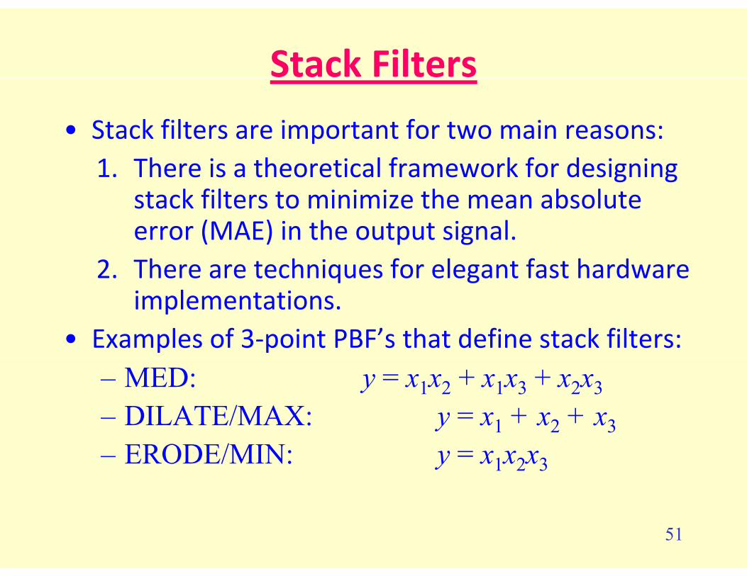
• Stack filters are important for two main reasons:1. There is a theoretical framework for designing

stack filters to minimize the mean absolute error (MAE) in the output signal.

2. There are techniques for elegant fast hardware implementations.

• Examples of 3-point PBF’s that define stack filters:– MED: y = x1x2 + x1x3 + x2x3– DILATE/MAX: y = x1 + x2 + x3y 1 2 3– ERODE/MIN: y = x1x2x3

51

Morphological Filters as Stack Filtersp g

• Because ERODE and DILATE are stack filters, so are OPEN, CLOSE, Close-Open, and Open-Close.

• This is the “detailed version” of what is meant by the figure on page 6.42.

• Ex: OPEN(x[n],B) with B=ROW(3):– Because OPEN(x[n],B) = DILATE[ERODE(x[n],B)],

this is actually a 5-point filtering operation.

– The PBF for the binary filters is given byy = x1x2x3 + x2x3x4 + x3x4x5

• It takes a lot more work to derive the PBFs for CLOSE, Close-Open, and Open-Close.

52

C OS , C ose Ope , Ope C ose.

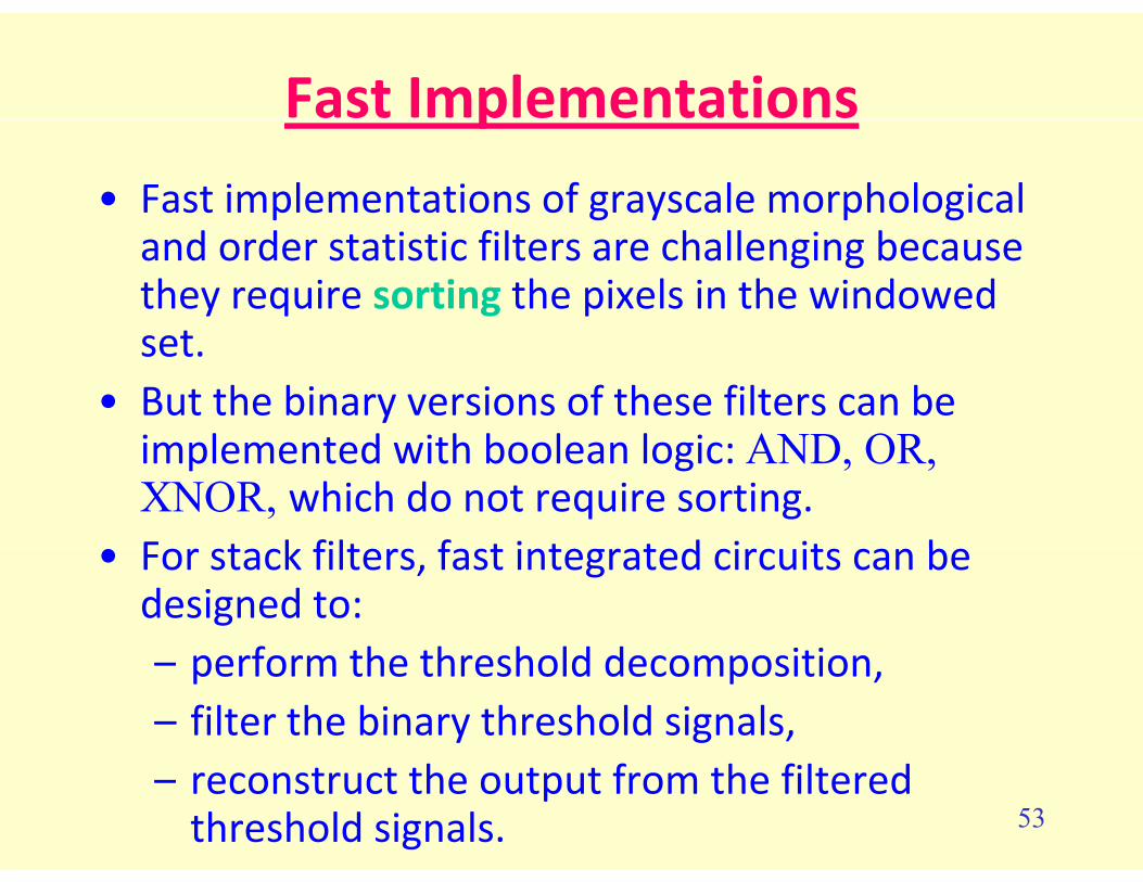
Fast Implementationsp

• Fast implementations of grayscale morphological and order statistic filters are challenging because they require sorting the pixels in the windowed

tset.• But the binary versions of these filters can be

i l t d ith b l l i AND ORimplemented with boolean logic: AND, OR, XNOR, which do not require sorting.F t k filt f t i t t d i it b• For stack filters, fast integrated circuits can be designed to:

perform the threshold decomposition– perform the threshold decomposition,– filter the binary threshold signals,

53– reconstruct the output from the filtered

threshold signals.

Fast Sortingg• Sorting is an expensive operation, especially for large

i d iwindow sizes.• Let M be the number of pixels in the windowed set.• Time complexity of common sorting algorithms:• Time complexity of common sorting algorithms:

– (M2): quicksort, insertion sort, selection sort…– (M logM): merge sort heapsort introsort(M logM): merge sort, heapsort, introsort…

• In hardware, space complexity can often be traded one-for-one for time complexity.

• If the binary version of the filter is a PBF, then there are very fast bit-serial realizations that require only B clock c clescycles.

54

Bit-Serial Median Filtering

• This algorithm is due to Delman (Proc. SPIE, vol. 298, 1981, pp. 184-188).pp )

• For an image I, suppose we want to implement the filter J= MED(I,B) with B = CROSS(5).( , ) ( )

• Suppose B=3-bit pixels and let the windowed set be

BI(i j) {2 0 1 5 6}BI(i, j) = {2, 0, 1, 5, 6}.• The median is 2.

With d ti h d• With good sorting hardware,– insertion sort requires at least 25 clock cycles.

merge sort requires at least 15 clock cycles– merge sort requires at least 15 clock cycles.• The bit-serial algorithm finds the median in only three clock

cycles!

55

y

First Clock Cycle y• Take the majority of the hi-order

bits. This is the hi-order bit of th di ( i thi )

0 1 0Original Data

the median (a zero in this case).• Any pixel with a hi-order bit of

one is bigger than the median

0 0 00 0 1 one is bigger than the median.

– Changing it to all ones will not change the median.

1 0 11 1 0

• This is the First Change, which is clocked into the registers by the rising edge of the second clock

Majority0 − −

First Change rising edge of the second clock cycle.0 1 0

0 0 0

First Change

0 0 00 0 11 1 1

561 1 1

Second Clock Cycle y• Take the majority of the second

bits. This is the second bit of the di ( i thi )

0 1 0First Change

median (a one in this case).• Any pixel with a second bit of

zero is smaller than the median

0 0 00 0 1 zero is smaller than the median.

– Changing it to all zeros will not change the median.

1 1 11 1 1

• This is the Second Change, which is clocked into the registers by the rising edge of

Majority01−

Second Change registers by the rising edge of the third clock cycle.0 1 0

0 0 0

Second Change

0 0 00 0 01 1 1

571 1 1

Third Clock Cycle y• Take the majority of the lo-order

bits. This is the lo-order bit of th di ( i thi )

0 1 0Second Change

the median (a zero in this case).• We are done! The median is

found in only three clock cycles!

0 0 00 0 0 found in only three clock cycles!

• This approach was generalized by Chen to develop fast bit-serial

1 1 11 1 1

realizations for any stack filter (IEEE Trans. Circuits, Syst., vol. 36 no 6 June 1989 pp 785-

Majority010

36, no. 6, June 1989, pp. 785794).

• For B-bit input pixels, each output pixel is computed in onlyB clock cycles.

58

ORDER STATISTIC FILTERSORDER STATISTIC FILTERS

59

ORDER STATISTIC FILTERS

• Recall the OS of a set X = {X1 ,..., X2P+1}:X {X X }XOS = {X(1) ,..., X(2P+1)}

such that

X(1) ≤ · · · ≤ X(2P+1).• Define a linear combination of order statistics

( )2P+1

Tp OSp

p=1A X = A X

where A = [A1 ,..., A2P+1]T. This defines a class of nonlinear filters called order statistic (OS) filters.

60

OS Filter Coefficients

• The filter weights are assumed to sum to 1:

2P+1T

pA 1= = A e

where e = [1, 1, ..., 1]T. Then if X = c·e is constant

p=1

then ATXOS = c, and the filter is then level-preserving – like a low-pass linear filter.

• The OS coefficients are assumed symmetric:Ai = A2P+2-i for 1 ≤ i ≤ 2P+1 61

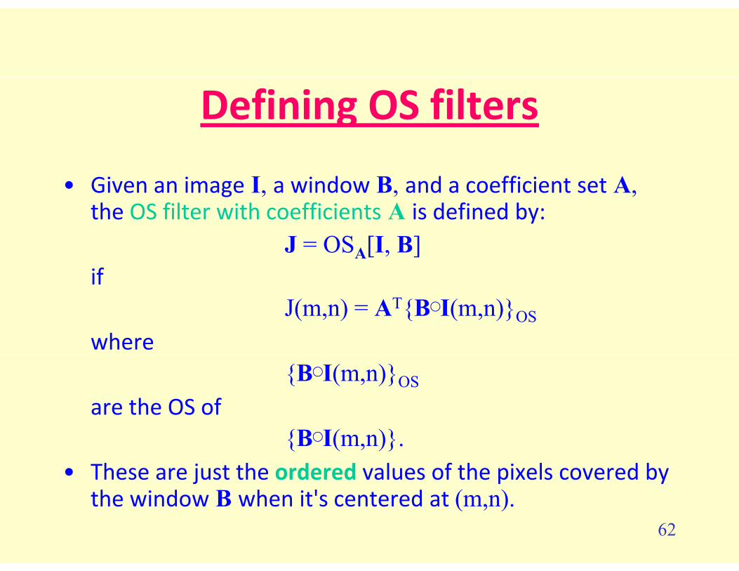
Defining OS filters

• Given an image I, a window B, and a coefficient set A, the OS filter with coefficients A is defined by:the OS filter with coefficients A is defined by:

J = OSA[I, B]if

J(m,n) = AT{BI(m,n)}OS

where{BI(m,n)}OS

are the OS of{BI(m,n)}.

• These are just the ordered values of the pixels covered by th i d B h it' t d t ( )

62the window B when it's centered at (m,n).

General Properties of OS Filters

• The behavior of a filter OSA[I, B] is largely d i d b i ffi i Adetermined by its coefficients A.

• Some important OS filters OSA[I, B] are:

- A = [0 0 1 0 0]T - median filterA [0 ,…, 0, 1, 0 ,..., 0] median filter

A filtT1 1 - A = - average filter1 1,...,

2P+1 2P+1

63

Median-Like OS Filtersll f h ff h l• Generally, if the coefficients A are concentrated near the middle:

0.4

0.5

A

0.1

0.2

0.3A p

then OSA[I B] is much like a median filter:

9876543210.0

then OSA[I, B] is much like a median filter:- preserve edges well- smooth noise

reduce impulses- reduce impulsesBUT

- will not "streak" or "blotch" as muchill i l i b ( l )

64- will suppress non-impulse noise better (more later)

Average-Like OS Filters• Generally, if the coefficients are widely distributed:

0.15

A p0.05

0.10

then OSA[I, B] will act much like an average filter:987654321

0.00

- preserve edges poorly (better than AVE)- smooth noise

blur impulses (not as badly as AVE)- blur impulses (not as badly as AVE)

• We will now explore the utility of these filters relative to some

65

p yof the noise models we have looked at.

OS Filter Design Criterion

• The goal of a smoothing filter can be stated asd h i ireduce the noise variance.

• OS filters are best characterized by their ability to reduce noise variance.

• For certain well-known noise PMFs, specific choices of the coefficients A of OSA[J, B] result using the variance reduction criterion.

66

Gaussian Noise – Average Filter

• The average filter is best among all OS filters at reducing Gaussiannoise variance. It is also the best linear filter. In fact, it is the best filt f ki d!filter of any kind!

• If B contains 2P+1 elements, then AVE[J, B] reduces (divides) the i f G i i b f tvariance of Gaussian noise by a factor

2P+1• In fact, AVE[J, B] reduces the variance of any white noise by a

factorfactor2P+1

• This is pretty good, but for non-Gaussian PMFs other OS filters can do much bettermuch better.

• Major caveat: The above does not account for the effect on the signal Average filtering blurs the signal as it reduces noise so there

67

signal. Average filtering blurs the signal as it reduces noise, so there exists a tradeoff between noise reduction and signal blurring.

Laplacian Noise – Median Filter

• The median filter MED[J, B] is the asymptotically best OS filter for reducing the variance of Laplacian noise (as window size increases).

• If B contains 2P+1 elements, then MED[J, B] reduces Laplaciannoise variance by a factor of (approximately)

2·(2P+1) - quite an improvement!

• MED[J, B] is fantastic for removing salt-and-pepper noise. No better filter!

• If the noise is Gaussian, then MED[J, B] reduces the noise variance by a factor of (approximately) only

(0.75)·(2P+1) - not an improvement!

68• Extended Caveat: The median filter is noted to not blur images, even

as the window size increases.

Median Filter vs. Average Filter

• Owing to its very important edge-preserving property, MED is generally regarded as superior to AVE (or anyMED is generally regarded as superior to AVE (or any other linear filter!) for reducing white noise in images.

• However, as with any application, care should be taken in analyzing the situation rather than blindly

l i filapplying a filter.

B h MED d AVE d f f i• Both MED and AVE are used far too often in situations where a design process might be more advantageous

69

advantageous.

Robust OS Filter Coefficients

• A fairly sophisticated statistical analysis yields the best OSAfilter for specific noise and image modelsfilter for specific noise and image models.

• Fortunately, a great property of certain OS filters is the fact y, g p p ythat they are robust.

• A filter is robust if it gives close to optimal performance for a wide variety of noise types.

• OS filters OSA have been shown to be remarkably robust for coefficients A that resemble a cross between MED and

70

coefficients A that resemble a cross between MED and AVE.

Trimmed Mean Filters

• A simple robust OS filter class is the trimmed mean OS filters TMQ[J, B] with coefficients

1 1 T

2(P-Q)+1 2(P-Q)+1Q Q

2(P Q)+1

= 0 ,..., 0, ,..., , 0,..., 0[ ]A

where Q < P (usually Q ≈ P/2).

2(P-Q)+1

• Similar to AVE since the innermost 2(Q-P)+1 OS are averaged. If Q = 0, then TMQ[J, B] = AVE[J, B].

• Similar to MED since only inner OS are averaged, the rest of the OS being “trimmed.” Indeed, if Q = P, then TMQ[J, B] = MED[J, B].

71

Trimmed Mean Filter Performance

• Trimmed mean filters smooth noise well (including impulse and Gaussian noise) and preserve edges wellimpulse and Gaussian noise) and preserve edges well.

F b h G i d L l i i TM d• For both Gaussian and Laplacian noise, TMP/2 reduces the variance by a factor

(0 9) OPTIMAL> (0.9)·OPTIMAL

where OPTIMAL is (2P+1) for Gaussian noise and 2·(2P+1) for Laplacian noise.

72

Generalized Gaussian PDF• The generalized gaussian PDF is used to model wide

behaviors of noise:

- x/σf (x) = K e - < x <γ

γ ∞ ∞

• For γ < 1, fγ(x) is very heavy-tailed.

( )γ

• For γ = 1, f1(x) is laplacian.

• For γ = 2, f2(x) is gaussian.

• As γ → ∞, f∞(x) is uniform.

• For a wide range of values of γg γTMP/2 > (0.9)·OPTIMAL! 73

Example – AWGN / S&P Noise

Time-consuming!G d lGood examples:N=3, SQUARE, P=2N = 5, CROSS, P=3AWGN with S&P

AWGN and S&P Noise 50% Trimmed Mean

74

BILATERAL FILTERBILATERAL FILTER

75

BILATERAL FILTERBILATERAL FILTER• Another principled approach to image denoising• Another principled approach to image denoising.

• Like OS filters, it modifies linear filtering.

• Like OS filters, it seeks to smooth while retaining(edge) structures.(edge) structures.

76

Bilateral Filter Concept• Observation: 2-D linear filtering is a method of

Bilateral Filter ConceptObservation: 2 D linear filtering is a method of weighting by spatial distances [i = (i, j), m = (m, n)]:

( )GJ ( ) = I( )G −m

i m m i

• If linear filter G is isotropic, e.g., a 2-D gaussian LPF*

( )2 2 2G(i j) K exp i j / = + σ

then is Euclidean distance

( )G GG(i, j) K exp i j / = − + σ

( ) ( )2 2m i + n j=m ithen is Euclidean distance.( ) ( )m-i + n-j− =m i

77*The value of KG is such that G has unit volume.

Bilateral Filter Concept• New idea: Instead of weighting by spatial distance,

Bilateral Filter ConceptNew idea: Instead of weighting by spatial distance, weight by luminance similarity

( ) ( )HJ ( ) = I( ) H I I− m

i m m i

• NOT a linear filter operation. H could be a 1-D gaussian weighting function*

2 2H HH(i) K exp i / = − σ

• Not very useful by itself.

78*The value of KH is such that H has unit area.

Bilateral Filter Definition• Combine spatial distance weighting with luminance

Bilateral Filter DefinitionCombine spatial distance weighting with luminance similarity weighting:

( ) ( ) ( )J( ) = I( )G H I I− − m

i m m i m i

• Computation is straightforward and about twice as

m

expensive as just spatial linear filtering.

• However, this can be sped up by pre-computing all values of H for every pair of luminances andvalues of H for every pair of luminances, and storing them in a look-up table (LUT). 79

Examplep

• Noisy edge filtered by bilateral filter (Tomasi, ICCV 1998).y g y ( , )

d i i il i• Uses gaussian LPF and gaussian similarity

Bilateral weighting 2 pixels to right of edge

Before After

80

pixels to right of edge

Color Examplep• Can extend to color using 3-D similarity weighting.

• If I = [R, G, B], then use

H[R(m)-R(i), G(m)-G(i), B(m)-B(i)][ ( ) ( ), ( ) ( ), ( ) ( )]where ( )2 2 2 2

H HH(i, j, k) K exp i j k / = − + + σ

Before After

81

Comments on Bilateral Filter• Similar to median filter, emphasizes luminances close in

l t t i lvalue to current pixel.

• Does not have a statistical (or other) design basis, so best used with care, e.g., retouching or low-level noise g gsmoothing.

• The idea of doing linear filtering that is decoupled near edges is very powerfuledges is very powerful.

• This is also the theme of the next method.82

NON LOCAL (NL) MEANSNON-LOCAL (NL) MEANS

83

NL Means Conceptp• Idea: Estimate the current pixel luminance as a

weighted average of all pixel luminances

• The weights are decided by neighborhood luminance similarityluminance similarity.

Th i h h f i l i l• The weight changes from pixel to pixel.

• In all the following, i = (i, j), m = (m, n), p = (p, q).

• The method is expensive but effective. 84

NL Means Conceptp• Given a window B, compute the luminance similarity

of every windowed set BI(i) with every otherof every windowed set BI(i) with every other windowed set BI(m):

( ) ( ) 2W WW( , ) K exp / = − − σ i m B I i B I m

where

( ) ( ) ( ) ( ) 2I I

∈

− = − − − p B

B I i B I m i p m p

( ) ( ) 2

(p,q)

I i p, j q I m p,n q∈

= − − − − − B

85

(p,q)∈B

j

Moderately

( )B I iiModerately

similar

HighlyHighlysimilar

Moderatelysimilar

Highlydissimilar

86

NL Means Definition

Gi i d B d th i hti f ti W j t• Given a window B, and the weighting function W just defined, the NL-means filtered image I is

( ) ( ) ( )W , I=m

J i m i m

• Thus each pixel value is replaced by a weighted sum ofall luminances where the weight increases withall luminances, where the weight increases with neighborhood similarity.

87

Example

Before AfterBefore After

88Difference

Example

Before After

89Difference

Comments• NL-Means is very similar in spirit to frame averaging.

• The main drawback is the large computation / search.

• It can be modified to compare/search less of theiimage.

• It works best when the image contains a lot of• It works best when the image contains a lot of redundancy (periodic, large smooth regions, textures).

• It can fail at unique image patches.

90

ANISOTROPIC DIFFUSIONANISOTROPIC DIFFUSION

91

ANISOTROPIC DIFFUSION

• A powerful approach to both image denoisingd d d t tiand edge detection.

• Fact: Gaussian blur or smoothing is analogous to physical diffusion (e.g., of heat).physical diffusion (e.g., of heat).

I f h i f i i l i• In fact the gaussian function is a solution to a PDE called the diffusion equation.

92

Concept of Anisotropic Diffusionp p

• Diffuse (smooth image pixels) where the gradient• Diffuse (smooth image pixels) where the gradient magnitude is small.

• Inhibit diffusion where gradient magnitude is large.g g g• Anisotropic since smoothing depends on direction.• Convolution with a Gaussian is isotropic diffusion.p

• Rationale:- Smooth image without destroying image detail- Inhibit smoothing across edges (inter-region g g ( gsmoothing)- Encourage smoothing between edges (intra-region

h )93

smoothing)

The Diffusion Equation • Continuous Formulation - a system of partial

differential equations:

[ ]2 2

EWEW NS2 2

NS

c 0I(x, y) I(x, y)div c c =0 ct x y

∂ ∂ ∂= ∇ = + ∂ ∂ ∂

I c I c

where I is the image, c is a 2x2 matrix of diffusioncoefficients, and div is the divergence operator

• The discrete formulation is much easier to understand...

Note: Recall

9411 22

ff fdiv( )fx y ∂ ∂= + = ∂ ∂

F Fwhere

A i i D i iApproximating Derivatives∂I

where time t will be iteration number of the

t 1 tI ( , ) I ( , )t

m n m n+∂ → −∂I

where time t will be iteration number of the diffusion process.

2

2I(x, y) I(m, n+1) - 2I(m, n) + I(m, n-1)x

∂ →∂

2

2I(x, y) I(m+1, n) - 2I(m, n) + I(m-1, n)y

∂ →∂

which approximates twice derivatives by twice

95differences.

Diffusion Equation: Discrete Form

• Iterative approximation using differences:

(2) (2)t 1 t NS t EW tEWNS

1I ( , ) I ( , ) c ( , ) I ( , ) c ( , ) I ( , )4

m n m n m n m n m n m n+ = + ∇ + ∇

where

t 1 t NS t EW tEWNS( ) ( ) ( ) ( ) ( ) ( )4+

where ... (2)NS I ( , ) I( , 1) - 2I( , ) I( , -1)t m n m n m n m n∇ = + +

N t If th th diff i ti b th h t ti

(2)EWI ( , ) I( 1, ) - 2I( , ) I( -1, )t m n m n m n m n∇ = + +

2∂∇

I

96

Note: If cNS = cEW = c, then the diffusion equation becomes the heat equation ct

= ∇∂

I

Diffusion Coefficients

• Selection of the diffusion coefficients cNS, cEW is important Usually cNS = cEWimportant. Usually cNS cEW.

• The idea is to inhibit smoothing over edgesThe idea is to inhibit smoothing over edges, encourage smoothing on non-edge image regions. So cNS, cEW should be edge-sensitive.

• At each pixel I(i, j), diffusion proceeds in a given di i di h diff i ffi idirection according to the diffusion coefficient corresponding to that direction and that location.

97

Diffusion Coefficients• One popular form

2 d2I( , )

d kc ( , ) exp d = NS, EWm nm n ∇ = −

where k is an edge threshold – as the gradient increases, cd rapidly falls.

• Properties of cd(m, n):- approaches 0 near edges – disenabling diffusionapproaches 0 near edges disenabling diffusion- approaches 1 over smooth areas –enabling

diffusion

98

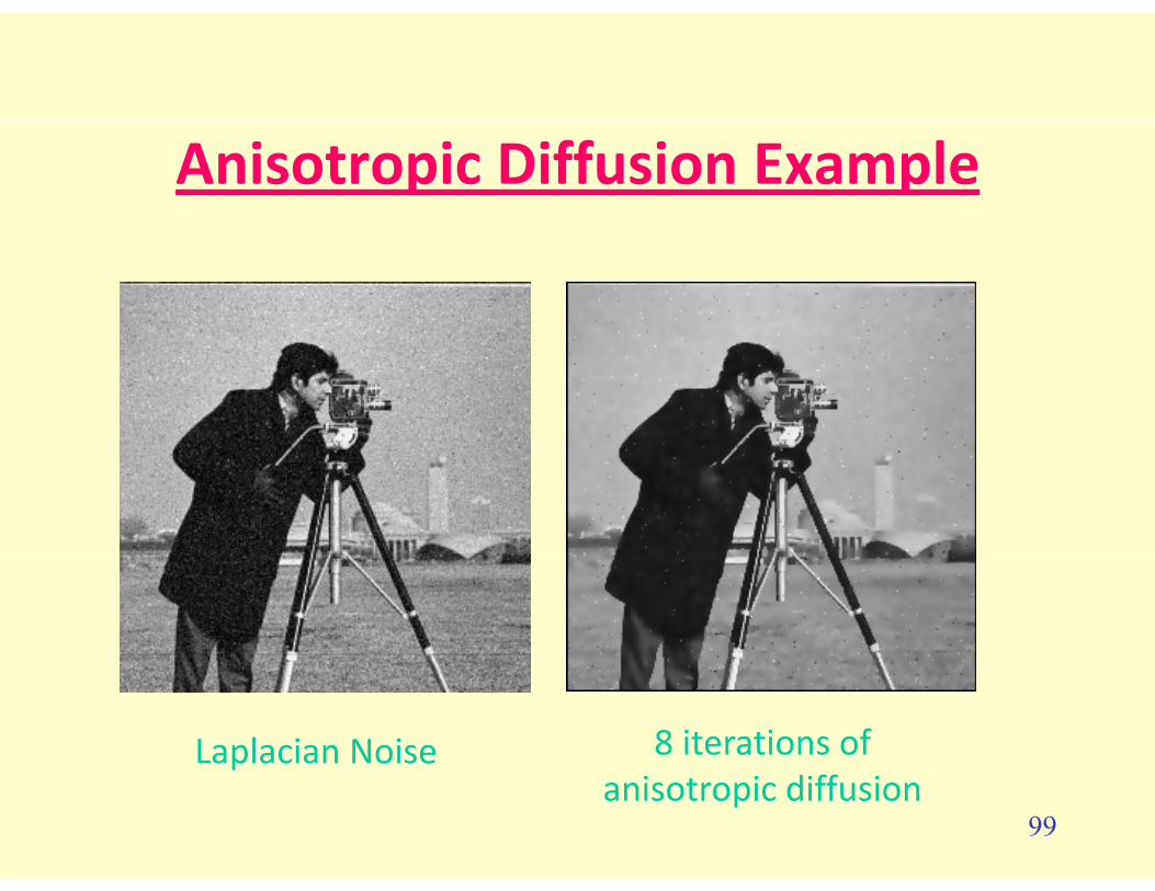
Anisotropic Diffusion Example

Laplacian Noise 8 iterations of

99anisotropic diffusion

Comments on Anisotropic Diffusion

• Really a method of alternating edgeReally a method of alternating edge detection with edge-decoupled smoothing.

• Number of iterations controls degree of h ( l )smoothing (scale)

• Edge detection applied to the smoothed image can be quite effective

100

image can be quite effective.

Comparisonp

AWGN Gaussian filtered Anisotropic diffusion

101Bilateral filtered NL-Means

WAVELET SHRINKAGEWAVELET SHRINKAGE

102

Wavelet ShrinkagegPerfect reconstruction analysis/synthesis filterbank or DWT

H 0 D G 0U0

H 1

I

D G 1U

ImageI

G

Σ

U

I

HP -1 D P -1 GU

Denoise the DWT coefficients

103

Wavelet ShrinkageWavelet Shrinkageh

Hig

h

H1 2 G12

IIm

age Σ

2

Iow

H1

Hig

h

ghH0

2 G1

Σ G02

2

2

Lo

H0

Low

H0

H1Hig

w2

H

22 G1

G0

Σ G0

Σ G22

2

HLow G

104Denoise the DWT coefficients

Wavelet Shrinkage

• The process of denoising is accomplished simply by

Wavelet Shrinkage

• The process of denoising is accomplished simply by thresholding the DWT coefficients (filter responses).

• A threshold is applied (p ≠ 0 since baseband signal is smooth already):smooth already):

Hp D tty (i)y (i)Hp D t py (i)py (i)

105

Wavelet Soft Thresholding• Two methods of thresholding:

H d h h ld i l d if b l h h ld– Hard threshold: signal zeroed if below threshold

– Soft threshold, where in addition to hard threshold, the threshold is subtracted if above thresholdthreshold is subtracted if above threshold.

Hard threshold Soft threshold

p ptp

y (i) ; if y (i) > ty (i) =

0 ; if y (i) t

≤

{ }tp p py (i) = sgn y (i) max 0, y (i) t −

p0 ; if y (i) t≤

t-t

t-t

106

Wavelet Shrinkage

• Soft thresholding is much more effective. It “shrinks” the wavelet coefficients.

• Works since additive noise increases ffi i f h h ldi dcoefficient energy. Soft thresholding reduces

the energy.

Th h ld b h t ti i• Threshold can be chosen to optimize many criteria such as MSE, Bayesian risk, etc.

107

Wavelet Shrinkage

• MMSE threshold (“SureShrink”)

where σ2 = estimated noise variance and NM =t = 2 log NMσ

where σ2 = estimated noise variance, and NM = # pixels in the image.

• Bayesian threshold (an SNR) (“BayesShrink”)

is estimated for each filter response (band)signal noiset = /σ σ

is estimated for each filter response (band), hence adaptive. When SNR is large, little th h ldi Wh l h th h ldithresholding. When large, heavy thresholding.

108

Wavelet Shrinkage ExamplesOriginal Noisy

SureShrink BayesShrink

109

DWT Used• There is no clear choice (yet) on wavelet filters to use.

• Here we used a 4-level DWT with the “Daubechies 10” orthogonal wavelet (D10)

Analysis LP Synthesis HPSynthesis LPAnalysis HPG0(0) = 0.0033357253G0(1) = -0.0125807520G0(2) = -0.0062414902G0(3) = 0.0775714938

G1(0) = -0.1601023980G1(1) = 0.6038292698G1(2) = -0.7243085284G (3) = 0 1384281459

H0(0) = 0.1601023980H0(1) = 0.6038292698H0(2) = 0.7243085284H (3) = 0 1384281459

H1(0) = 0.0033357253H1(1) = 0.0125807520H1(2) = -0.0062414902H (3) = 0 0775714938 0( )

G0(4) = -0.0322448696G0(5) = -0.2422948871G0(6) = 0.1384281459G0(7) = 0.7243085284

G1(3) = 0.1384281459G1(4) = 0.2422948871G1(5) = -0.0322448696G1(6) = -0.0775714938G (7) = 0 0062414902

H0(3) = 0.1384281459H0(4) = -0.2422948871H0(5) = -0.0322448696H0(6) = 0.0775714938H (7) = 0 0062414902

H1(3) = -0.0775714938H1(4) = -0.0322448696H1(5) = 0.2422948871H1(6) = 0.1384281459H (7) = 0 7243085284 G0(7) 0.7243085284

G0(8) = 0.6038292698G0(9) = 0.1601023980

G1(7) = -0.0062414902G1(8) = 0.0125807520G1(9) = 0.0033357253

H0(7) = -0.0062414902H0(8) = -0.0125807520H0(9) = 0.0033357253

H1(7) = -0.7243085284H1(8) = 0.6038292698H1(9) = -0.1601023980

110

Comments

• Since DWTs can be computed very fast, so can soft threshold based denoising.

• The results are optimal in wavelet space and the bl dappearance is reasonably good.

111

BM3DBM3D

112

Overview

• Quite a complicated algorithm – too much! Uses many of the ideas we have covered

• Image broken into blocks blocks thenmatchedImage broken into blocks, blocks thenmatchedby similarity into groups.

ll b i l f d f h• Estimates are collaboratively formed for each block within each group.

• This is done by a transformation of the group and a shrinkage processand a shrinkage process.

• Perhaps the best denoising algorithm extant.

Dabov, Foi, Katkovnik, Egiazarian, IEEE Trans on Image Processing, Aug 2007.113

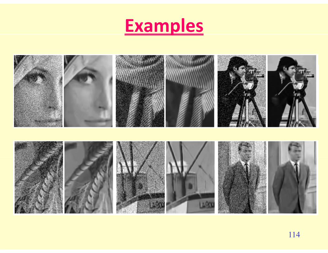
Examplesp

114

HOMOMORPHIC FILTERING

• Assume a multiplicative white noise model:J = I ⊗ NJ = I ⊗ N

where I is the original image and N is a white noise imageimage.

• ThusThusJ(m,n) = I(m,n)N(m,n) for 0 ≤ m ≤ M-1, 0 ≤ n ≤ N-1.

• Direct linear filtering ineffective, since the noise / image spectra not added.

115

g p

Multiplicative Noise

• Multiplicative noise is always positive since the sensed image intensities must be.g

• Multiplicative noise often has an exponential PMF in practical applications such as radar laser based imagingpractical applications, such as radar, laser-based imaging, electron microscopy, etc.

• Synthetic aperture radar images are an excellent example.

• Multiplicative noise appears much worse in bright image regions (since it multiplies the gray levels) and can be h dl i bl d k

116hardly noticeable in dark regions.

Homomorphic Approach

• Homomorphic filtering is succinctly expressed by the following diagram:

noisyimage

J

logarithmicpoint operation

log(·)

linear ornonlinear

filter

exponentialpoint operation

exp(·)

smoothedimage

K

• We'll study each step:

J K

• We ll study each step:

117

Logarithmic Point Operation

• Idea is similar to log point operations used for histogram improvement: de-emphasize dominant bright image pixels.

• More than that! Since log (a·b) = log (a) + log (b), then

log [J(m n)] = log [I(m n)] + log [N(m n)]log [J(m,n)] = log [I(m,n)] + log [N(m,n)].

• So: the point operation converts the problem into that of smoothingJ´ I´ + N´J = I + N

whereI´(m,n) = log [I(m,n)], N´(m,n) = log [N(m,n)], J´(m,n) = log [J(m,n)]

• Importantly, N´ is still a white noise image.

• This is just the additive white noise problem studied earlier!

118

• This is just the additive white noise problem studied earlier!

Filtering

• The filtering problem here is very similar to the linear and nonlinear ones studied earlier in this Module and in Module 5.

• Depending on the noise statistics, AVE, MED, OSA, OPEN-CLOSE, CLOSE-OPEN or other linear or nonlinear filter may be used.

• The theoretical performance of these various filters in homomorphicsystems still remains an open question.

• Most will work reasonably well; in particular MED has been observedto be effective if the noise is exponential and the image contains edgesedges.

• The objective is of course to produce a filtered result

119F[J´, B] ≈ I´

Exponential Point Operation

• If the filtering operation succeeds:

F[J´, B] ≈ I´

then the output image K will approximate

K(i, j) ≈ exp [I´(i, j)]I(i j)= I(i, j)

120

Comments

• We shall now study some BIG topics –image quality and compression onwardimage quality and compression… onward to Module 7..

121